NOVEL RECTANGULAR SPIRAL ANTENNAS

A Thesis Submitted to the Graduate School of Engineering and Sciences of

İzmir Institute of Technology in Partial Fulfillment of the Requirements for the Degree of

MASTER OF SCIENCE

in Electronics and Communication Engineering

by Uğur SAYNAK

October, 2007 İZMİR

We approve the thesis of Uğur SAYNAK

_______________________ Assist. Prof. Dr. Alp KUŞTEPELİ Supervisor _______________________ Assoc. Prof. Dr. Thomas F. BECHTELER Committee Member _______________________ Assoc. Prof. Dr. Taner OĞUZER Committee Member 19. October 2007 Date __________________________ _______________________________ Prof. Dr. F. Acar SAVACI Prof .Dr. Hasan BÖKE Head of Department of Electrical and Dean of the Graduate School of Electronics Engineering Engineering and Sciences

iii

ABSTRACT

NOVEL RECTANGULAR SPIRAL ANTENNAS

Round spiral antennas are generally designed by using Archimedean spiral geometries

which have linear growth rates. To obtain smaller antennas with nearly the same

performance, square spiral Archimedean geometries are also widely used instead. In this

study, novel square antennas are proposed, designed and examined. At first two similar

but different approaches are employed to design new antennas by considering the design

procedure used to obtain log-periodic antennas. Then, the performance of these

antennas is improved by considering another property of log-periodic antennas.

Simulations are performed by using two different numerical methods which are Finite

Difference Time Domain Method (FDTD) and Method of Moments (MoM). The results

obtained from the simulations are compared with those of the Archimedean spiral

antennas in terms of the frequency dependency of fundamental antenna parameters such

as antenna gain and radiation pattern. The simulation results are compared with the ones

obtained from the experimental study.

iv

ÖZET

YENİ DİKDÖRTGEN SPİRAL ANTENLER

Dairesel spiral antenler genellikle doğrusal oranlarla açılan Arşimet spiral eğrileri

biçiminde tasarlanırlar. Benzer performanslı çalışabilen daha küçük antenler elde etmek

için kare Arşimet geometrileri yaygın olarak kullanılırlar. Bu çalışmada, yeni kare spiral

anten tasarımları önerilmiş, tasarlanmış ve incelenmiştir. İlk çift yeni antenin

tasarımında log-periyodik anten tasarımında kullanılan yöntem göz önüne alınarak iki

benzer ama farklı yaklaşım kullanılmıştır. Daha sonra bu iki geometri log-periyodik

antenlerin başka bir özelliği kullanılarak geliştirilmeye çalışılmıştır. Benzetimler biri

FDTD metodu diğeri Moment metodu olmak üzere farklı iki yöntemle yapılmıştır. Yeni

tasarımların benzetim sonuçları Arşimet antenlerin sonuçlarıyla temel anten

parametrelerinin frekansa bağımlılığı açısından karşılaştırılarak incelenmiştir. Ayrıca

benzetim sonuçları deney sonuçlarıyla karşılaştırılarak bir kıyaslama yapılmıştır.

v

TABLE OF CONTENTS

LIST OF FIGURES ........................................................................................................vii

CHAPTER 1 INTRODUCTION ...................................................................................... 1

CHAPTER 2 SPIRAL ANTENNAS................................................................................ 4

2.1. Archimedean Spiral ................................................................................ 4

2.2. Rumsey’s Scaling Principle .................................................................... 5

2.3. Logarithmic Spiral .................................................................................. 6

2.4. Radiating Ring Theory............................................................................ 7

2.5. Comparison of Square and Round Geometries....................................... 7

CHAPTER 3 ANTENNA GEOMETRIES..................................................................... 10

3.1. Log periodic antenna geometries .......................................................... 10

3.2. Proposed Geometries ............................................................................ 11

3.3. Radiation Mechanism of Proposed Geometries.................................... 12

CHAPTER 4 NUMERICAL METHODS ...................................................................... 14

4.1. Simulation Procedure............................................................................ 14

4.2. The Method of Moments ...................................................................... 14

4.3. The Finite-Difference Time-Domain Method ...................................... 16

4.4. Comparison of Results Obtained by the Finite-Difference Time-Domain Method and the Method of Moments........................... 19

CHAPTER 5 RESULTS AND DISCUSSIONS ............................................................ 21

5.1. Simulation Parameters .......................................................................... 21

5.2. Gain and Axial Ratio Comparisons ...................................................... 21

5.3. Radiation Patterns ................................................................................. 26

5.4. Structure Complexity versus Frequency Dependency.......................... 26

5.5. Effect of a Possible Dielectric Support ................................................. 29

vi

5.6. Measurement Procedure and Results .................................................... 32

CHAPTER 6 CONCLUSION ........................................................................................ 35

REFERENCES ............................................................................................................... 36

vii

LIST OF FIGURES

Figure Page

Figure 2.1. Archimedean spirals (a) round (b) square…………………………………...5

Figure 2.2. Radiating rings on a square spiral geometry………………………………...7

Figure 2.4. (a) Square Archimedean and round spiral (b) Square

Archimedean and round spiral with smaller radius.…………………….......8

Figure 2.5. Comparison of gains of square and round spiral geometries………………..9

Figure 3.1. A Simple Log-Periodic Antenna (Log-periodic Dipole antenna).…………10

Figure 3.2. Geometries…………………………………...…………………………….11

Figure 3.3. Configuration of Geometry B…………………………………...................12

Figure 3.4. Four LPDA elements………………………………….................................13

Figure 4.1. Time Domain Port Current for a Dipole Antenna………………………….18

Figure 4.2. Real Input Impedance Comparison of a 15 cm Dipole…………………….20

Figure 4.3. Imaginary Input Impedance Comparison of a 15 cm Dipole………………20

Figure 5.1. Gain Comparison of 3 turn Archimedean Geometry A and

Geometry B (MoM Results).……………………………….....................22

Figure 5.2. Axial Ratio Comparison of 3 turn Archimedean Geometry

A and Geometry B (MoM Results)……...………………………………...22

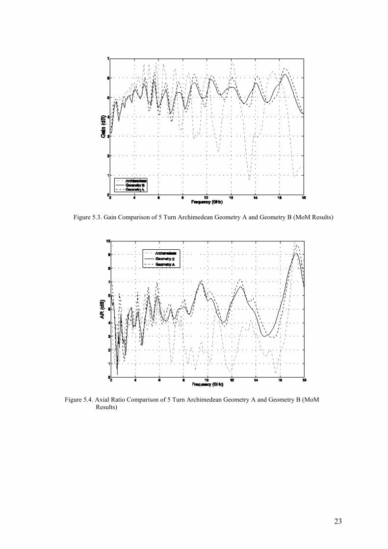
Figure 5.3. Gain Comparison of 5 Turn Archimedean Geometry A and

Geometry B (MoM Results)………...………………………………...…...23

Figure 5.4. Axial Ratio Comparison of 5 Turn Archimedean Geometry A

and Geometry B (MoM Results)……...…………………………………...23

Figure 5.5. Gain Comparison of 7 Turn Archimedean Geometry A

and Geometry B (MoM Results) ……………………..…………………...24

Figure 5.6. Axial Ratio Comparison of 7 Turn Archimedean Geometry A

and Geometry B (MoM Results)………………………………………...24

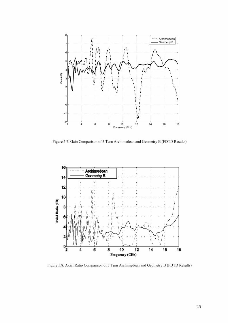
Figure 5.7. Gain Comparison of 3 Turn Archimedean and Geometry B

(FDTD Results).……………………………………………………………25

Figure 5.8. Axial Ratio Comparison of 3 Turn Archimedean and

Geometry B (FDTD Results).………………………………………………25

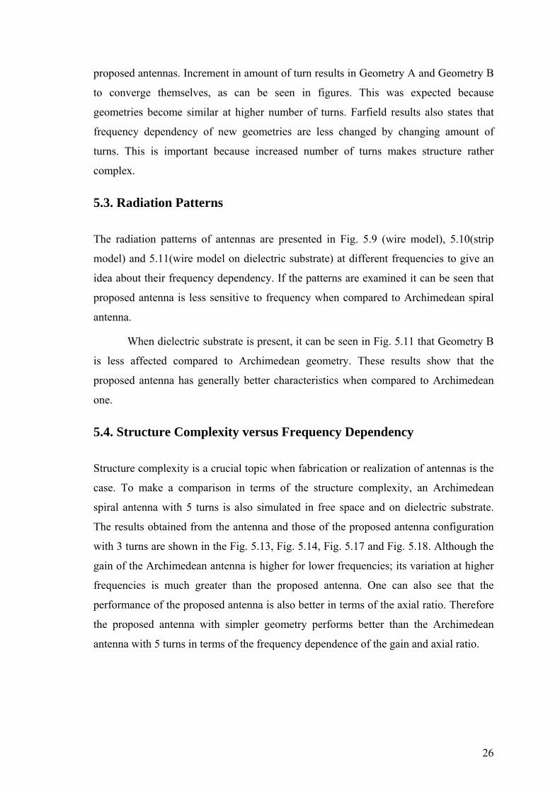
Figure 5.9. Radiation Pattern Comparison of Archimedean (dashed)

viii

and Geometry B (dash-dot) (MoM results)……..………………………27

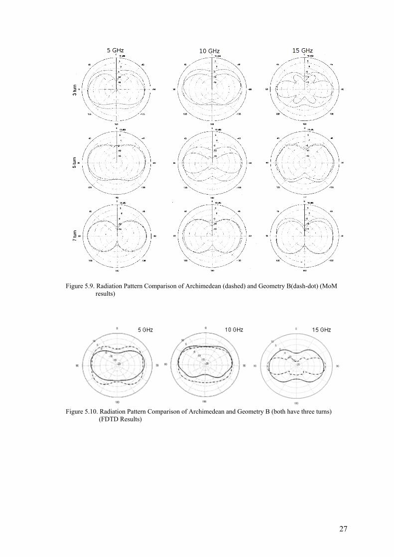
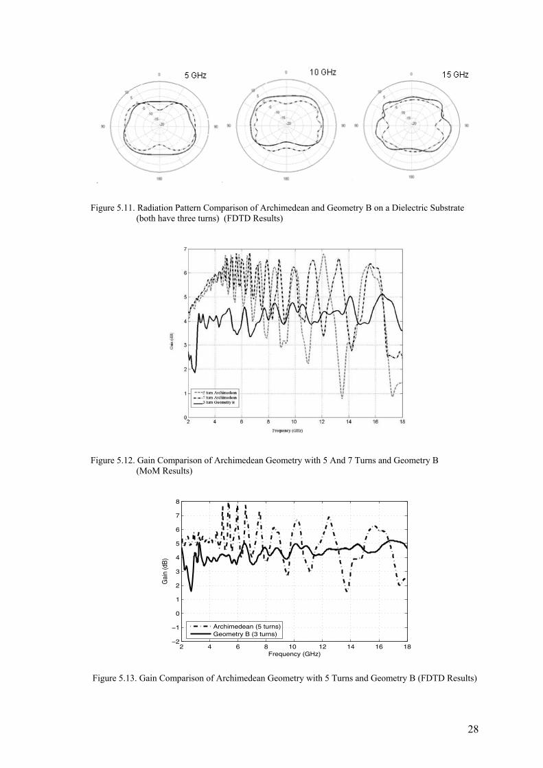
Figure 5.10. Radiation Pattern Comparison of Archimedean and Geometry

B (both have three turns) (FDTD Results)……...…...……………………27

Figure 5.11. Radiation Pattern Comparison of Archimedean and

Geometry B on a Dielectric Substrate (both have

three turns) (FDTD Results)..……………………………………………28

Figure 5.12. Gain Comparison of Archimedean Geometry with 5 And

7 Turns and Geometry B (MoM Results)…………………...……………28

Figure 5.13. Gain Comparison of Archimedean Geometry with 5 Turns

and Geometry B (FDTD Results) ………………………………………...28

Figure 5.14. Axial Ratio Comparison of Archimedean Geometry

With 5 turns and Geometry B (FDTD Results)……...……………………29

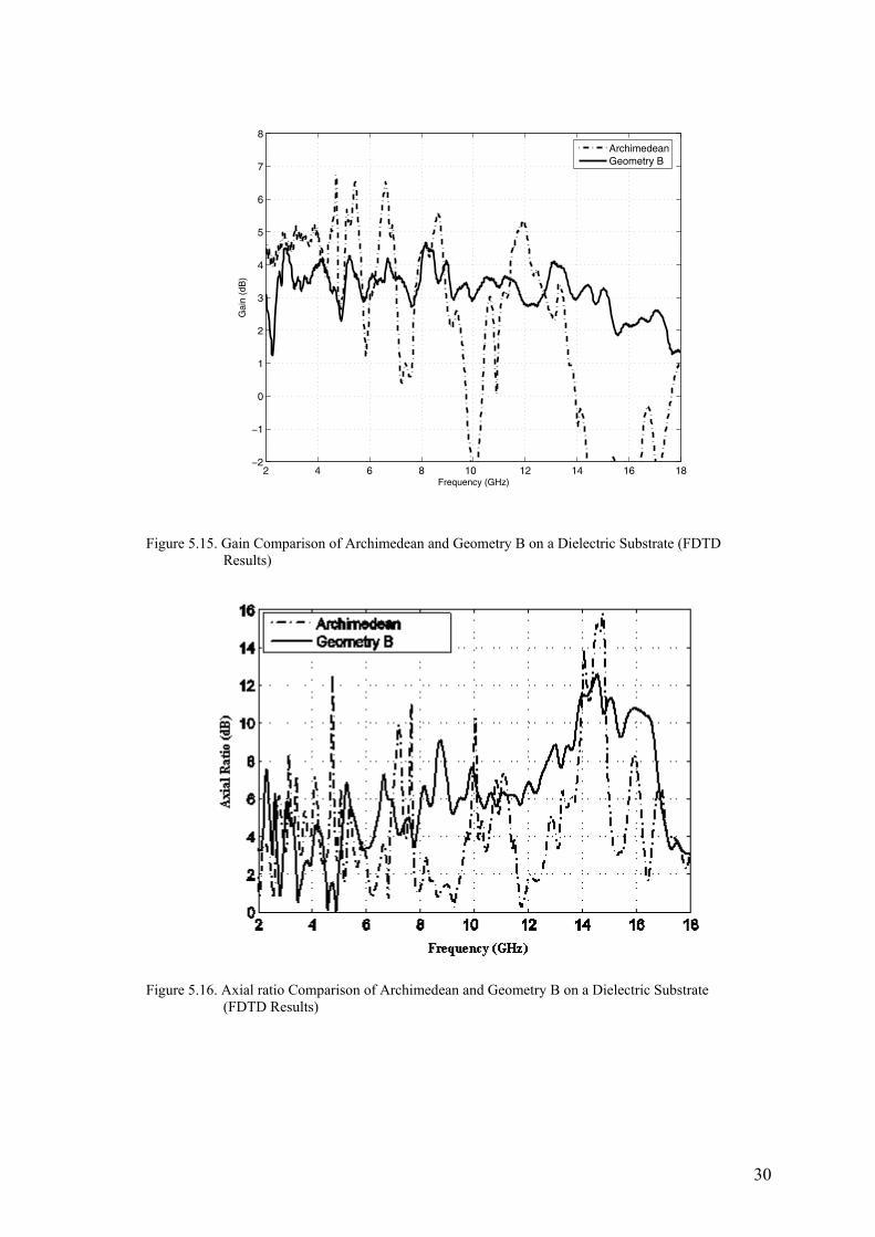
Figure 5.15. Gain Comparison of Archimedean and Geometry B on a

Dielectric Substrate (FDTD Results)…………………………………...…30

Figure 5.16. Axial ratio Comparison of Archimedean and Geometry

B on a Dielectric Substrate (FDTD Results).………..……………………30

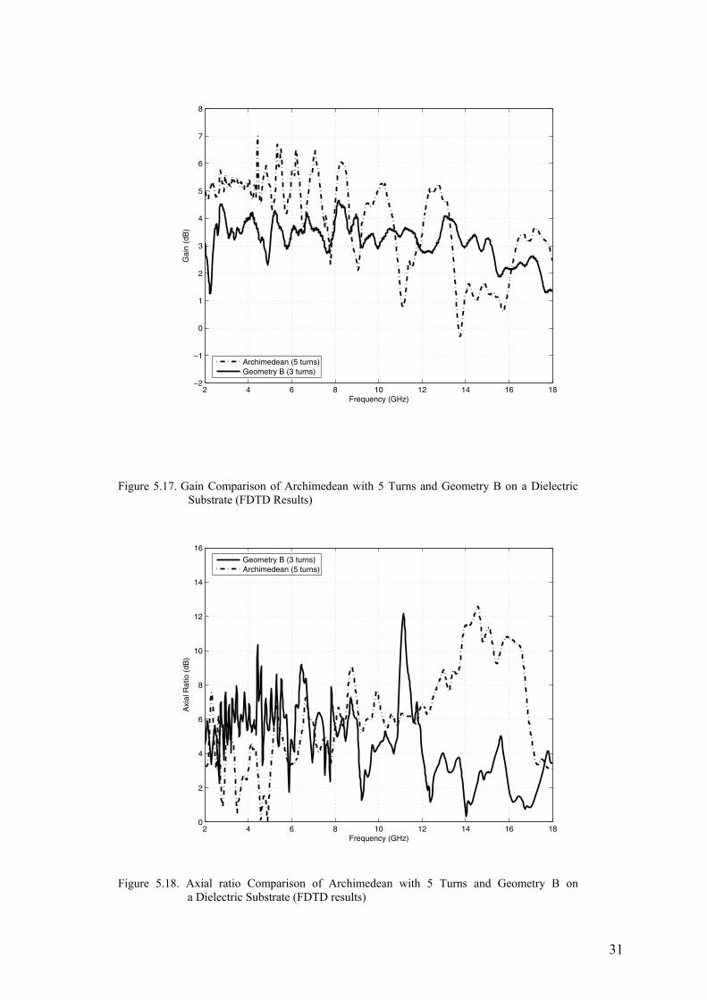
Figure 5.17. Gain Comparison of Archimedean with 5 Turns and

Geometry B on a Dielectric Substrate (FDTD Results).………….………31

Figure 5.18. Axial ratio Comparison of Archimedean with 5 Turns

and Geometry B on a Dielectric Substrate (FDTD results).……………...31

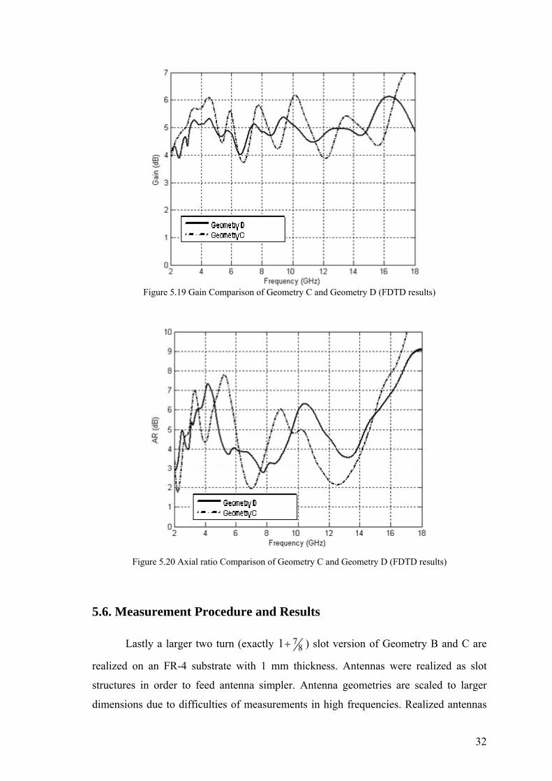
Figure 5.19 Gain Comparison of Geometry C and Geometry D (FDTD

results).……………………………………………………………………32

Figure 5.20 Axial ratio Comparison of Geometry C and Geometry

D (FDTD results).…………...…………………………………………….32

Figure 5.21. Comparison of S11 values of Geometry B and C………………………...33

Figure 5.22. Comparison of Measured and Simulated VSWR Values of

Geometry C………………………………...……………………………..34

Figure 5.23. Comparison of Measured and Simulated Impedance Values

of Geometry C…………………………………………………………….34

1

CHAPTER 1

INTRODUCTION

Since investigation of the Hertz dipole, antennas and communication systems

are improving day by day. Today we need wide bandwidths, smaller antennas and wider

coverage. Especially modern mobile devices’ need of these kinds of antennas is

increasing rapidly. At earlier years, interference was a crucial problem in

communication, due to primitive solid state technology. This restriction led to narrower

bandwidths, and different kind of polarizations (for instance whereas AM radio

channels use vertical polarization, analog TV channels use horizontal polarization).

After research studies led investigation of modern solid state devices like semiconductor

transistors, restrictions like interference started not to be important in communication

and related topics. Increase of demand on all in one devices and information

technologies, raised the need of low-cost, compact, wideband, omnidirectional and low-

power antennas.

After investigation of log-periodic antennas at 1940’s, they were classified as

frequency independent antennas because of their bandwidths as wide as 1:40. This

foundation led to scaling principle, which explained operation theory of spiral antennas,

investigated at mid 1950’s.

Frequency independent antennas are used in applications requiring very wide

bandwidths (Kramer 2005, Filipovic 2002, Nurnberger 2000, Iwasaki 1994, Brown

2006, Ely 1995, Filipovic 2002, Ely 1995, Sevgi 2006, Bell 2004). These types of

antennas have fundamental characteristics which do not change much with frequency.

But this independency is limited to a band of frequency determined by antenna size

(Dyson 1959, Balanis 1997, Gloutak 1997). Since spiral antennas can be constructed as

planar structures and radiate circularly polarized waves, they are widely used when

compared to the others. They can be used for electronic countermeasures (ECM),

surveillance, remote sensing (Ground Penetrating Radar etc.), direction finding (Global

Positioning System etc.), telemetry, and flush mounted airborne applications. Spiral

2

antennas can be used as a separate component antenna or as broadband feeds for

reflector type dish antennas.

Due to their characteristics of quite broad bandwidths and circular polarization

(CP) (Dyson 1954) spiral antennas are widely used for instance as broadband or

narrowband radiators in mobile-communication, early-warning, and direction-finding

systems, in addition to some other applications. In the recent past many planar spiral

antennas have been analyzed under various conditions; spirals in free space (Kaiser

1960, Curtis 1960, Gloutak 1997), spirals on planar reflectors (Wang 1991, Nakano

1986), spirals on dielectric substrates (Nakano 2004, Nakano 2002, Penney 1994) and

spirals in cavities (Kramer 2005, Iwasaki 1994, Nurnberger 2000, Filipovic 2002,

Kramer 2005) and the effects of the number of turns, number of arms, arm lengths,

increments, plate distance, and so forth on radiation performance have been

documented. The shape of a spiral radiator can be Archimedean (Curtis 1960), or

logarithmic (Wang 1991). Spiral antennas are designed and fabricated in round or

square geometries. When the first radiation bands of the circular and square spiral

antennas are examined one can see that the square spiral antennas have the advantage of

operating with the same performances at lower frequencies (Kramer 2005, Bawer

1960). But at high frequencies square geometries seems to be less frequency

independent (Caswell 2001)

In this study novel square-spiral antennas is designed which are more frequency

independent than square Archimedean ones. To have such an antenna a new geometry is

obtained by employing the design method of log-periodic antennas. In this work the

proposed antennas and equivalent sized Archimedean spiral antennas are first analyzed

and compared in free-space then also a dielectric substrate is added to examine the

effect of the support of antennas. The simulations are performed firstly by using

Moment Method as wire structures, afterwards using Finite Difference Time Domain

method (FDTD) as strip structures. Then FDTD simulations are also verified by

experimental results. Most of the results are presented for a comparison especially in

terms of frequency dependency of the fundamental antenna parameters. Gain, axial ratio

and radiation patterns for a frequency band from 2-18 GHz are characterized and

discussed. Also impedance characteristics are analyzed and verified by experimental

study. Frequency dependency of new antenna types is better at especially second half of

3

the frequency band compared with Archimedean square spiral antennas. Also antenna

parameters at lower frequencies are characterized and compared with round and square

Archimedean spirals for size comparisons. Lastly experimental studies were carried out

for slot versions of geometry B and C to prove large impedance bandwidth of the

antennas. Measured wideband S11 results were compared with those of simulation

results show good agreement.

Organization of this document is as follows: in chapter 2 spiral antenna concepts

are introduced with theory, introduction of new antenna geometries is presented in

chapter 3, chapter 4 gives information about the numerical methods, in chapter 5

numerical and experimental results are presented and conclusion is given in chapter 6.

4

CHAPTER 2

SPIRAL ANTENNAS

2.1. Archimedean Spiral

Although Archimedean and logarithmic spirals have different equations defining

them, practice shows that their characteristics do not differ by very much. Although a

logarithmic spiral has more uniform characteristics over the entire frequency range, an

Archimedean spiral can be useful for dimension considerations (Bawer 1960).The

Archimedean spiral increases uniformly with the angle:

r a bϕ= + (2.1)

where r is the distance from the origin, b is the initial point and a is the growth rate.

The structure cannot be scaled to an infinitesimal size by using Eq. (2.1), one of the

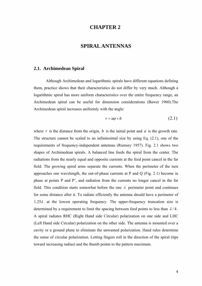
requirements of frequency-independent antennas (Rumsey 1957). Fig. 2.1 shows two

shapes of Archimedean spirals. A balanced line feeds the spiral from the center. The

radiations from the nearly equal and opposite currents at the feed point cancel in the far

field. The growing spiral arms separate the currents. When the perimeter of the turn

approaches one wavelength, the out-of-phase currents at P and Q (Fig. 2.1) become in

phase at points P and P’, and radiation from the currents no longer cancel in the far

field. This condition starts somewhat before the one λ perimeter point and continues

for some distance after it. To radiate efficiently the antenna should have a perimeter of

1.25λ at the lowest operating frequency. The upper-frequency truncation size is

determined by a requirement to limit the spacing between feed points to less than / 4λ .

A spiral radiates RHC (Right Hand side Circular) polarization on one side and LHC

(Left Hand side Circular) polarization on the other side. The antenna is mounted over a

cavity or a ground plane to eliminate the unwanted polarization. Hand rules determine

the sense of circular polarization. Letting fingers roll in the direction of the spiral (tips

toward increasing radius) and the thumb points to the pattern maximum.

5

Figure 2.1. Archimedean spirals (a) round (b) square

2.2. Rumsey’s Scaling Principle

Thinking of an antenna, whose geometry is described in spherical coordinates

( , , )r θ ϕ , has feed points infinitely close to the origin. It’s assumed that the antenna is

perfectly conducting; it is surrounded by an infinite homogeneous and isotropic

medium, and its surface or just one element of surface described by a curve

( , )r F θ ϕ= (2.2)

scaling curve by a factor K means lowering operating frequency of the original

frequency by a factor K . Thus the new surface is described by

' ( , )r KF θ ϕ= (2.3)

The new and old surfaces are identical, if both surfaces are infinite. Examining the

geometries one can say that a rotation of one geometry can give other geometry. For the

scaled antenna to achieve transformation with the original one, it must be rotated by an

angle C so that

( , ) ( , )KF F Cθ ϕ θ ϕ= + (2.4)

The rotation angle C depends on K but neither depends on θ or ϕ . Physical

congruence implies that the original antenna electrically would behave the same at both

frequencies. However the radiation pattern will be rotated azimuthally through an

angleC . For unrestricted values of K ( 0 K≤ ≤ ∞ ), the pattern will rotate by C in ϕ

with frequency, because C depends on K , but its shape will be unaltered. Thus the

impedance and pattern will be frequency independent.

6

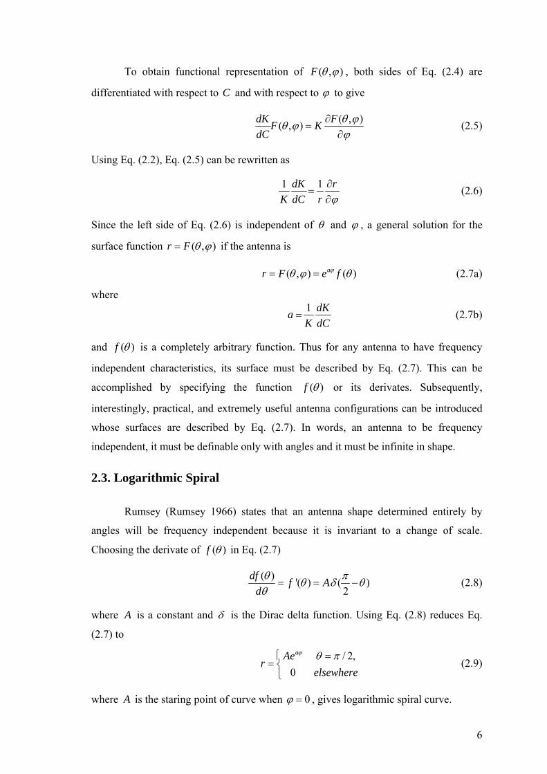
To obtain functional representation of ( , )F θ ϕ , both sides of Eq. (2.4) are

differentiated with respect to C and with respect to ϕ to give

( , )( , )dK FF KdC

θ ϕθ ϕϕ

∂=

∂ (2.5)

Using Eq. (2.2), Eq. (2.5) can be rewritten as

1 1dK rK dC r ϕ

∂=

∂ (2.6)

Since the left side of Eq. (2.6) is independent of θ and ϕ , a general solution for the

surface function ( , )r F θ ϕ= if the antenna is

( , ) ( )ar F e fϕθ ϕ θ= = (2.7a)

where

1 dKaK dC

= (2.7b)

and ( )f θ is a completely arbitrary function. Thus for any antenna to have frequency

independent characteristics, its surface must be described by Eq. (2.7). This can be

accomplished by specifying the function ( )f θ or its derivates. Subsequently,

interestingly, practical, and extremely useful antenna configurations can be introduced

whose surfaces are described by Eq. (2.7). In words, an antenna to be frequency

independent, it must be definable only with angles and it must be infinite in shape.

2.3. Logarithmic Spiral

Rumsey (Rumsey 1966) states that an antenna shape determined entirely by

angles will be frequency independent because it is invariant to a change of scale.

Choosing the derivate of ( )f θ in Eq. (2.7)

( ) '( ) ( )2

df f Adθ πθ δ θθ

= = − (2.8)

where A is a constant and δ is the Dirac delta function. Using Eq. (2.8) reduces Eq.

(2.7) to

/ 2,

0

aAer

elsewhere

ϕ θ π⎧ == ⎨⎩

(2.9)

where A is the staring point of curve when 0ϕ = , gives logarithmic spiral curve.

7

It is evident from Eq. (2.9) that changing the wavelength is equivalent to varying

ϕ which results nothing more than a pure rotation of the infinite structure pattern.

Within limitations imposed by the arm length and outer diameter, similar characteristics

have been observed for finite structures. Thus we have frequency independent antennas.

2.4. Radiating Ring Theory

A two-wire spiral antenna can be considered as a two-wire transmission line

which is gradually transformed into a radiating structure due to its expanding spiral

structure. A two-wire transmission line, of narrow spacing relative to the operation

wavelength and of any length, yields a negligible amount of radiation when excited.

This is due to the fact that the currents in the two wires of the line at any normal cross

section are always 180° out-of-phase at the operation frequencies so that radiation from

one line is effectively cancelled by the radiation from the other.

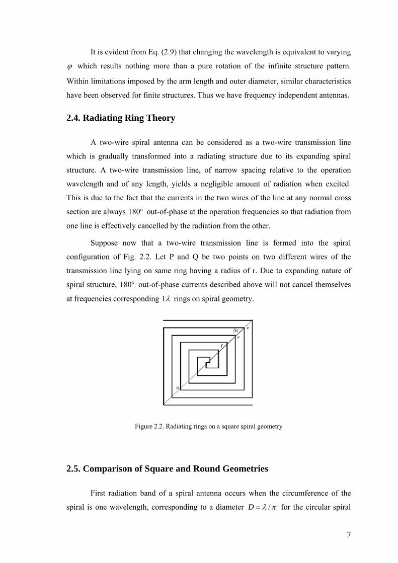
Suppose now that a two-wire transmission line is formed into the spiral

configuration of Fig. 2.2. Let P and Q be two points on two different wires of the

transmission line lying on same ring having a radius of r. Due to expanding nature of

spiral structure, 180° out-of-phase currents described above will not cancel themselves

at frequencies corresponding 1λ rings on spiral geometry.

Figure 2.2. Radiating rings on a square spiral geometry

2.5. Comparison of Square and Round Geometries

First radiation band of a spiral antenna occurs when the circumference of the

spiral is one wavelength, corresponding to a diameter /D λ π= for the circular spiral

8

and a width / 4W λ= for the square spiral. According to this relation, square spiral

geometries have more advantages in terms of size.

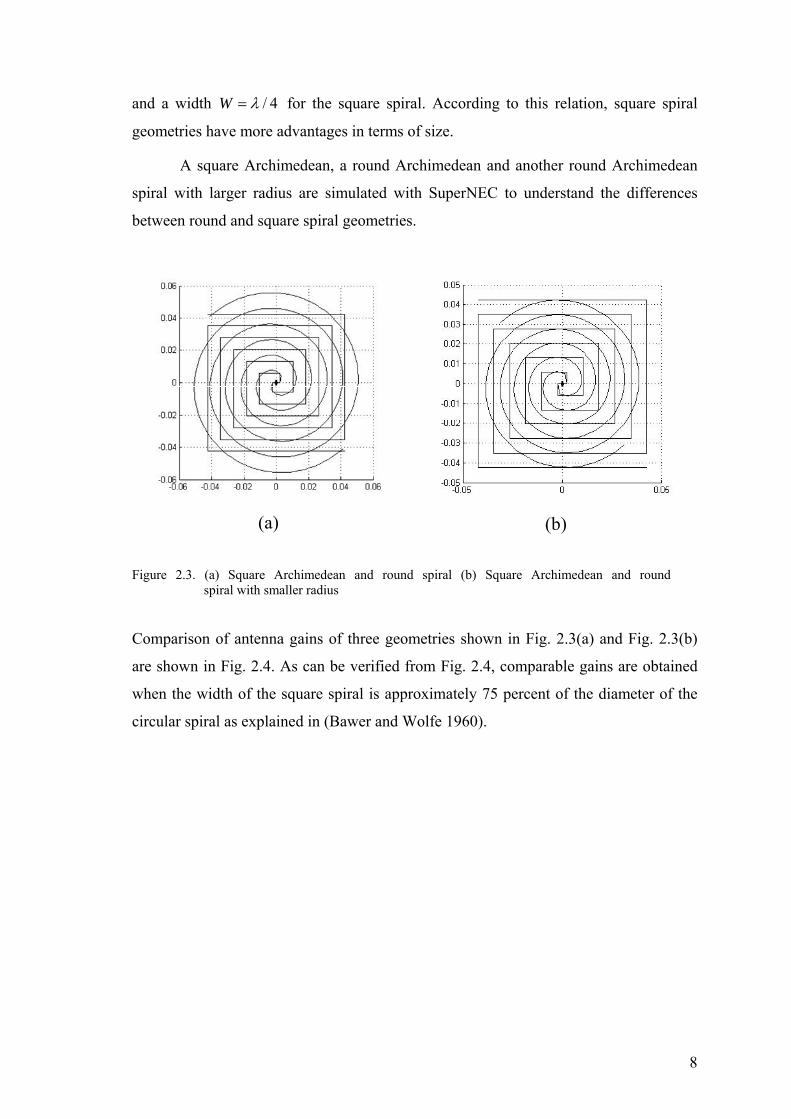
A square Archimedean, a round Archimedean and another round Archimedean

spiral with larger radius are simulated with SuperNEC to understand the differences

between round and square spiral geometries.

(a)

(b)

Figure 2.3. (a) Square Archimedean and round spiral (b) Square Archimedean and round

spiral with smaller radius

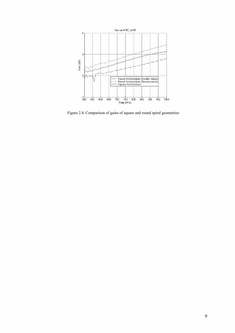
Comparison of antenna gains of three geometries shown in Fig. 2.3(a) and Fig. 2.3(b)

are shown in Fig. 2.4. As can be verified from Fig. 2.4, comparable gains are obtained

when the width of the square spiral is approximately 75 percent of the diameter of the

circular spiral as explained in (Bawer and Wolfe 1960).

9

Figure 2.4. Comparison of gains of square and round spiral geometries

10

CHAPTER 3

ANTENNA GEOMETRIES

3.1. Log Periodic Antenna Geometries

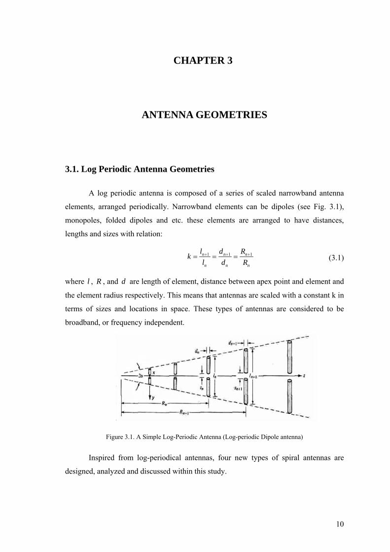
A log periodic antenna is composed of a series of scaled narrowband antenna

elements, arranged periodically. Narrowband elements can be dipoles (see Fig. 3.1),

monopoles, folded dipoles and etc. these elements are arranged to have distances,

lengths and sizes with relation:

1 1 1n n n

n n n

l d Rk

l d R+ + += = = (3.1)

where l , R , and d are length of element, distance between apex point and element and

the element radius respectively. This means that antennas are scaled with a constant k in

terms of sizes and locations in space. These types of antennas are considered to be

broadband, or frequency independent.

Figure 3.1. A Simple Log-Periodic Antenna (Log-periodic Dipole antenna)

Inspired from log-periodical antennas, four new types of spiral antennas are

designed, analyzed and discussed within this study.

11

3.2. Proposed Geometries

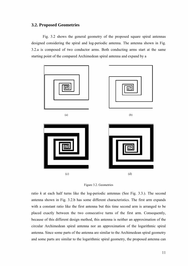
Fig. 3.2 shows the general geometry of the proposed square spiral antennas

designed considering the spiral and log-periodic antenna. The antenna shown in Fig.

3.2.a is composed of two conductor arms. Both conducting arms start at the same

starting point of the compared Archimedean spiral antenna and expand by a

(a) (b)

(c) (d)

Figure 3.2. Geometries

ratio k at each half turns like the log-periodic antennas (See Fig. 3.3.). The second

antenna shown in Fig. 3.2.b has some different characteristics. The first arm expands

with a constant ratio like the first antenna but this time second arm is arranged to be

placed exactly between the two consecutive turns of the first arm. Consequently,

because of this different design method, this antenna is neither an approximation of the

circular Archimedean spiral antenna nor an approximation of the logarithmic spiral

antenna. Since some parts of the antenna are similar to the Archimedean spiral geometry

and some parts are similar to the logarithmic spiral geometry, the proposed antenna can

12

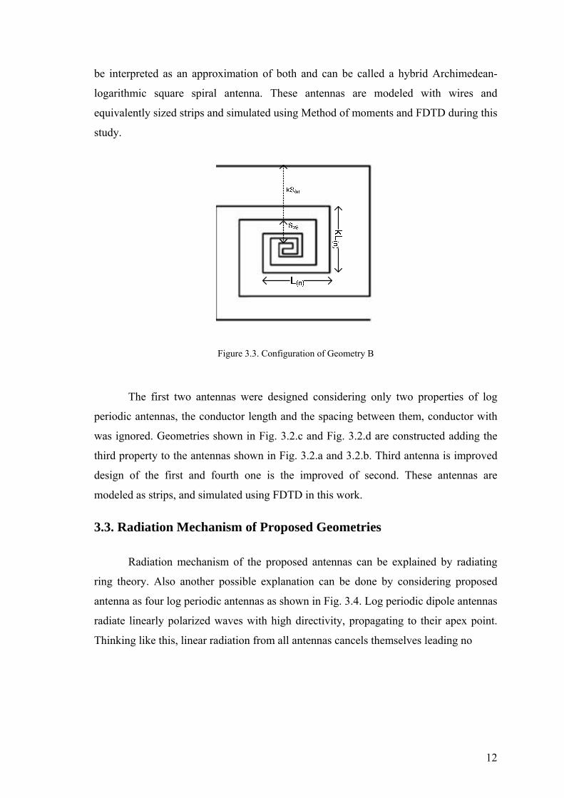
be interpreted as an approximation of both and can be called a hybrid Archimedean-

logarithmic square spiral antenna. These antennas are modeled with wires and

equivalently sized strips and simulated using Method of moments and FDTD during this

study.

Figure 3.3. Configuration of Geometry B

The first two antennas were designed considering only two properties of log

periodic antennas, the conductor length and the spacing between them, conductor with

was ignored. Geometries shown in Fig. 3.2.c and Fig. 3.2.d are constructed adding the

third property to the antennas shown in Fig. 3.2.a and 3.2.b. Third antenna is improved

design of the first and fourth one is the improved of second. These antennas are

modeled as strips, and simulated using FDTD in this work.

3.3. Radiation Mechanism of Proposed Geometries

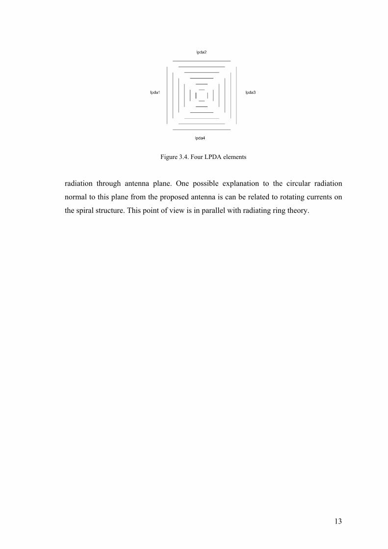
Radiation mechanism of the proposed antennas can be explained by radiating

ring theory. Also another possible explanation can be done by considering proposed

antenna as four log periodic antennas as shown in Fig. 3.4. Log periodic dipole antennas

radiate linearly polarized waves with high directivity, propagating to their apex point.

Thinking like this, linear radiation from all antennas cancels themselves leading no

13

Figure 3.4. Four LPDA elements

radiation through antenna plane. One possible explanation to the circular radiation

normal to this plane from the proposed antenna is can be related to rotating currents on

the spiral structure. This point of view is in parallel with radiating ring theory.

14

CHAPTER 4

NUMERICAL METHODS

4.1. Simulation Procedure

Numerical analysis is carried out using two different techniques, Method of

Moments and Finite Differences in Time Domain method. Moment method is used for

wire geometries especially for ease of use and accuracy for this type of structures.

FDTD is used for strip structures due to realization reasons, capability of modeling

complex geometries and broadband analysis advantage of this method.

4.2. The Method of Moments

The method of moments (MoM) is a general procedure for solving Equations of

type (4.1). The method owes its name to the process of taking moments by multiplying

with appropriate weighing functions and integrating. In general, method of moments is

used to solve integral equations which do not have analytical solution.

gL =Φ (4.1)

where L is an operator which may be differential, integral or integro-differential, g is

the known excitation or source function, and Φ is the unknown function to be

determined.

The procedure for applying MoM to solve Eq. (4.1) usually involves four steps:

1. Derivation of the appropriate integral equation (IE),

2. Conversion (discretization) of the integral equation into a matrix equation

using basis (or expansions) functions and weighting (or testing) functions,

3. Evaluation of the matrix elements, and

4. Solving the matrix equation and obtaining the parameters of interest.

15

The unknown function Φ may be expanded in a sum of basis functions, jφ , as :

1

Nj jj

α φ=

Φ =∑ (4.2)

A set of equations for the coefficients jα are then obtained by taking the inner

product of Eq. 4.1 with a set of weighting functions { }iω

, ,i iL gω ωΦ = (4.3)

Due to the linearity of L , substituting Eq. 4.2 for Φ yields,

1

, ,Nj i j ij

L gα ω φ ω=

=∑ (4.4)

This equation can be written in matrix notation as:

[ ][ ] [ ]G A E= (4.5)

where

, , , , ,i j i j j j i iG L A E gω φ α ω= = = (4.6)

The solution is then

[ ] [ ] [ ]1A G E−= (4.7)

and the integral equation to be solved is:

( ) ( ) ( ) ( )( ) ( )2 2ˆ ˆ g , '4 S

S

jn n k dAkηπ−

× = × +∇∫ir' E r r J r' r r' (4.8)

In this work commercial software which is an object oriented version of NEC2

FORTRAN code SuperNEC V2.7 is used for MoM simulations.

When the current distribution on geometry is calculated, far fields of this

geometry can be calculated. The far field data of the antennas are calculated using

standard far field approximations, such that

Tjω≅ −E A (4.9)

where TA is the transverse component of the magnetic vector potential, ω is the

angular frequency. The magnetic vector potential can be calculated as

ˆ ˆ( ) ( ') '4

jkrjkr r

S

er r e dSr

μπ

−− ⋅= ∫A J (4.10)

16

where ( ')rJ is the current density on structure, calculated by MoM, r̂ is the observation

direction vector and μ is magnetic permeability. When the antenna surface is PEC

there is no resistivity on the antenna, consequently the efficiency of the antenna is equal

to 1. The directivity of the antenna is calculated with the ratio of the radiation intensity

to the input power of the antenna.

( , )( , ) 4in

UDPθ φθ φ π= (4.11)

where

( ) ( )( )221( , ) , ,2

U E Eθ φθ φ θ φ θ φη

= + (4.12)

As shown in Eq. 4.12 the radiation intensity ( ),U θ φ (Watt/unit solid angle), is a

far field parameter and it can be calculated from both the polarization components of the

scattered electric field. Also the power supplied to the antenna inP is computed from the

applied voltage and computed current by numerical calculation.

4.3. The Finite-Difference Time-Domain Method

FDTD directly calculates Maxwell’s differential (curl) equations on spatial grids

or lattices in time-domain. The FDTD method, introduced by Yee in 1966, was the first

technique in this class, and has remained the subject of continuous development. Since

about 1990, when engineers in the general electromagnetics community became aware

of the modeling capabilities afforded by FDTD and related techniques, the interest in

this area has expanded.

FDTD simulations for this study are performed with rack server available in

Electric and Electronical Department of İzmir Institute of Technology which had a

RAM of 4 GB and two Intel Xeon processors during this study.

The choice of cell size is critical in applying FDTD. It must be small enough to

permit accurate results at the highest frequency of interest, and yet be large enough to

keep resource requirements manageable. Cell size is directly affected by the materials

present. The greater the permittivity or conductivity, the shorter the wavelength at a

given frequency and the smaller the cell size required. Generally it is chosen by the rule

17

smaller than one tenth of smallest wavelength (minimum wavelength is determined by

materials present in FDTD space and maximum interested frequency).

min10

λΔ ≤ (4.13)

Once the cell size is selected, the maximum time step is determined by the

Courant stability condition. Smaller time steps are permissible, but do not generally

result in computational accuracy improvements except in special cases. A larger time

step results in instability. In one dimensional FDTD space:

min max

tfλΔ

Δ ≤ (4.14)

where maxf is the maximum interested frequency in FDTD simulation and minλ is the

smallest wavelength in FDTD space. More generally for a three dimensional rectangular

grid:

( ) ( ) ( )

1

2 2 2min max

1 1 1 1tf x y zλ

−⎛ ⎞⎜ ⎟Δ ≤ + +⎜ ⎟Δ Δ Δ⎝ ⎠

(4.15)

When using the scattered field FDTD formulation the incident field must be

analytically specified. An infinite variety of waveforms are possible, but experience has

led to the Gaussian pulse as the incident waveform of choice. Also when strongly

resonant geometries (cavities etc.) are present, excitation of the FDTD in a narrower

frequency band by using modulated Gaussian waveform or excitation of single

frequency using sinusoidal waveform may be useful in increasing accuracy and

decreasing calculation time.

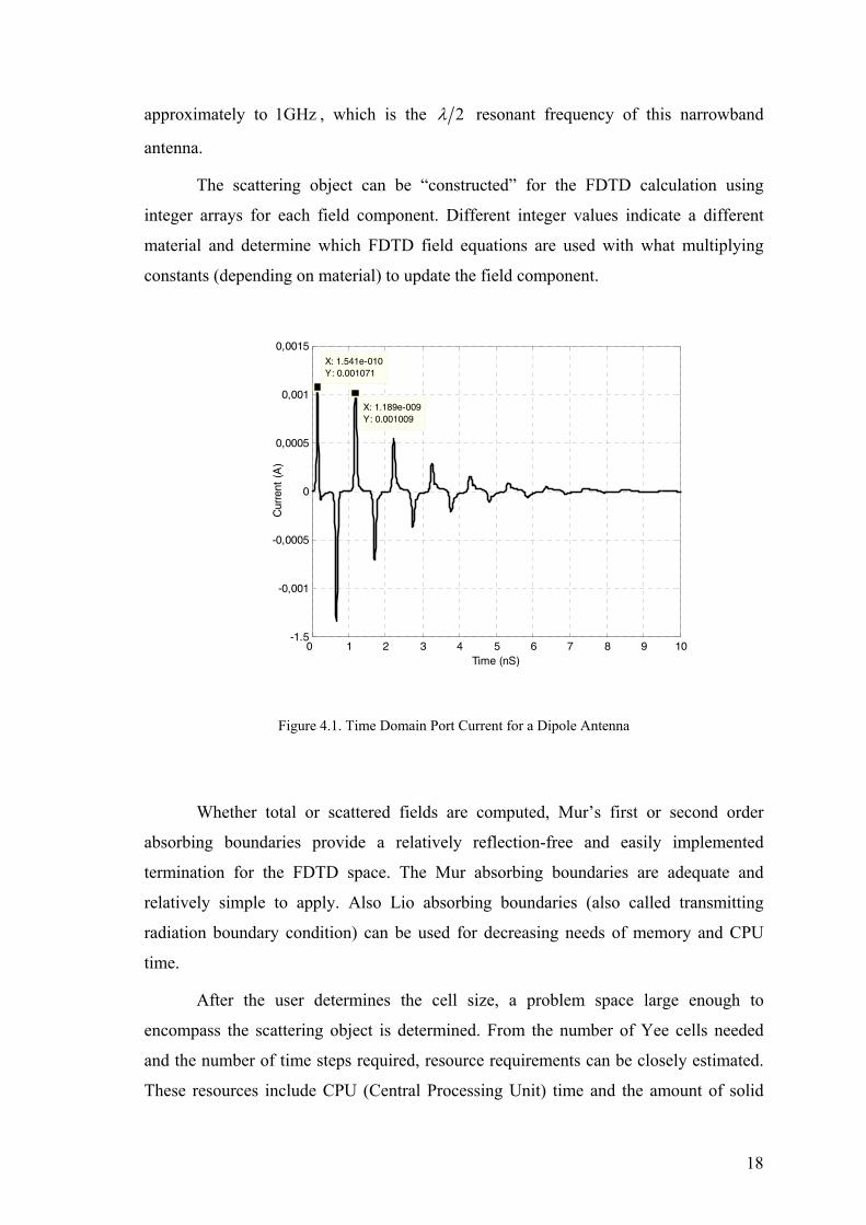
Ports are modeled as specified conductivity which correspond source resistance

and specified current or voltage waveforms at port locations considering a port as active

or passive. Port current and voltage values are calculated performing appropriate finite

integrations at port locations in time domain (See Fig 4.1). Then time domain values are

converted to frequency domain using FFT. For instance a dipole antenna having 15 cm

length was found to have a time domain port current as can be seen in Fig. 4.1.

Periodicity of this value is due to resonant characteristics of the dipole antenna. Time

differences between major peaks are found to be 1.0399 nS, corresponding

18

approximately to 1GHz , which is the 2λ resonant frequency of this narrowband

antenna.

The scattering object can be “constructed” for the FDTD calculation using

integer arrays for each field component. Different integer values indicate a different

material and determine which FDTD field equations are used with what multiplying

constants (depending on material) to update the field component.

0 1 2 3 4 5 6 7 8 9 10-1.5

-0,001

-0,0005

0

0,0005

0,001

0,0015

X: 1.189e-009Y: 0.001009

Time (nS)

Cur

rent

(A

)

X: 1.541e-010Y: 0.001071

Figure 4.1. Time Domain Port Current for a Dipole Antenna

Whether total or scattered fields are computed, Mur’s first or second order

absorbing boundaries provide a relatively reflection-free and easily implemented

termination for the FDTD space. The Mur absorbing boundaries are adequate and

relatively simple to apply. Also Lio absorbing boundaries (also called transmitting

radiation boundary condition) can be used for decreasing needs of memory and CPU

time.

After the user determines the cell size, a problem space large enough to

encompass the scattering object is determined. From the number of Yee cells needed

and the number of time steps required, resource requirements can be closely estimated.

These resources include CPU (Central Processing Unit) time and the amount of solid

19

state memory and extended storage capacity needed for the calculation and for storing

the results.

FDTD formulation is simple and geometry independent. After discretizating

problem geometry into cells, on every point of the grid, at every timestep Maxwell’s

equations are solved in differential form, with center, right and left differences rules.

Center differences formulation is can be seen in Eq. 4.16 for derivates of

function u with variable x , and derivates of function u with time in Eq. 4.17

1 2, , 1 2, ,, , ,n ni j k i j ku uu (i x j y k z n t)

x x+ −−∂

Δ Δ Δ Δ =∂ Δ

(4.16)

1 2 1 2

, , , ,, , ,n ni j k i j ku uu (i x j y k z n t)

t t

+ −−∂Δ Δ Δ Δ =

∂ Δ (4.17)

And applied Maxwell’s equations are in Eq. 4.18.

0

t tρ

∂ ∂− = ∇× − = ∇× −∂ ∂∇ ⋅ = ∇ ⋅ =

B DE M H J

D B (4.18)

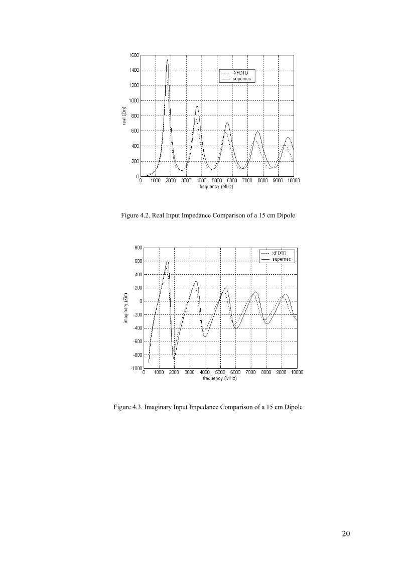
4.4. Comparison of Results Obtained by the Finite-Difference Time-

Domain Method and the Method of Moments

Primitive wire designs were analyzed using method of moments and then these

results are compared with those for equivalent strip structure’s (Equivalency is due to

Babinet principle) finite difference time domain method simulation results. In Fig. 4.2.

and Fig. 4.3. impedance versus frequency plots are presented for a dipole antenna with

15 cm length for comparison of wire and strip results. For dipole antenna MoM results

are considered as numerical exact solutions. Differences between FDTD and MoM are

related to model errors of FDTD for wire structures which have many approximations.

20

Figure 4.2. Real Input Impedance Comparison of a 15 cm Dipole

Figure 4.3. Imaginary Input Impedance Comparison of a 15 cm Dipole

21

CHAPTER 5

RESULTS AND DISCUSSIONS

5.1. Simulation Parameters

Equivalently sized different versions of Archimedean and proposed antennas are

simulated in free space and also on a dielectric substrate. They have an area of

8cm 8cm× for the free space simulations and their feed gap is equal to 4.6mm at their

centers. Antennas are firstly designed with 3, 5 and 7 turns corresponds exactly to 7

82+ , 784+ and 7

86+ turns respectively. For all of the simulations when the

dielectric substrate is present its thickness is equal to 1.6mm and its dielectric constant

is 2.2 . For MoM Simulations, antennas are modeled as wires with 0.1mm radius. Each

segment length is taken as 10Δ at the upper simulation frequency 18GHz (1.7 mm ).

For extended thin wire kernel model this values are quite acceptable at 2GHz 18GHz−

frequency band. For FDTD simulations, the cell size in the analysis is chosen equal to

the strip (infinitely thin) widths as 0.4mm for free space simulations. When the antenna

is supported by a dielectric substrate, in order to model dielectric substrate better, the

cell dimension along the substrate xΔ is decreased to 0.2mm (8 cells). The time step

values are also decreased to appropriate values according to the changed cell sizes.

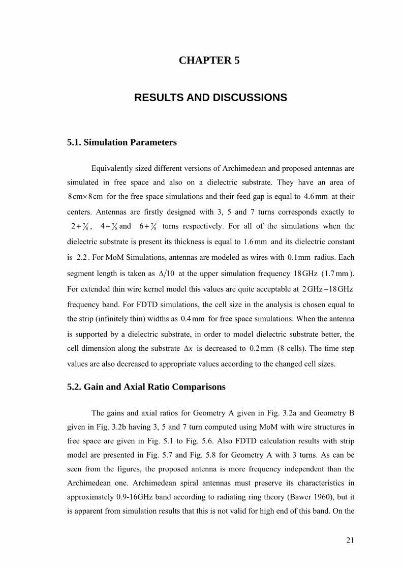
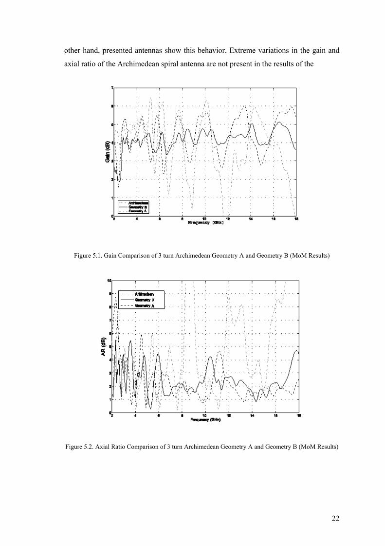
5.2. Gain and Axial Ratio Comparisons

The gains and axial ratios for Geometry A given in Fig. 3.2a and Geometry B

given in Fig. 3.2b having 3, 5 and 7 turn computed using MoM with wire structures in

free space are given in Fig. 5.1 to Fig. 5.6. Also FDTD calculation results with strip

model are presented in Fig. 5.7 and Fig. 5.8 for Geometry A with 3 turns. As can be

seen from the figures, the proposed antenna is more frequency independent than the

Archimedean one. Archimedean spiral antennas must preserve its characteristics in

approximately 0.9-16GHz band according to radiating ring theory (Bawer 1960), but it

is apparent from simulation results that this is not valid for high end of this band. On the

22

other hand, presented antennas show this behavior. Extreme variations in the gain and

axial ratio of the Archimedean spiral antenna are not present in the results of the

Figure 5.1. Gain Comparison of 3 turn Archimedean Geometry A and Geometry B (MoM Results)

Figure 5.2. Axial Ratio Comparison of 3 turn Archimedean Geometry A and Geometry B (MoM Results)

23

Figure 5.3. Gain Comparison of 5 Turn Archimedean Geometry A and Geometry B (MoM Results)

Figure 5.4. Axial Ratio Comparison of 5 Turn Archimedean Geometry A and Geometry B (MoM Results)

24

2 4 6 8 10 12 14 16 180

1

2

3

4

5

6

7

Frequency (GHz)

Gai

n (d

B)

ArchimedeanGeometry AGeometry B

Figure 5.5. Gain Comparison of 7 Turn Archimedean Geometry A and Geometry B (MoM Results)

2 4 6 8 10 12 14 16 180

1

2

3

4

5

6

7

8

9

10

Frequency GHz

AR

(dB

)

ArchimedeanGeometry AGeometry B

Figure 5.6. Axial Ratio Comparison of 7 Turn Archimedean Geometry A and Geometry B (MoM Results)

25

2 4 6 8 10 12 14 16 18−2

−1

0

1

2

3

4

5

6

7

8

Gai

n (d

B)

Frequency (GHz)

ArchimedeanGeometry B

Figure 5.7. Gain Comparison of 3 Turn Archimedean and Geometry B (FDTD Results)

Figure 5.8. Axial Ratio Comparison of 3 Turn Archimedean and Geometry B (FDTD Results)

26

proposed antennas. Increment in amount of turn results in Geometry A and Geometry B

to converge themselves, as can be seen in figures. This was expected because

geometries become similar at higher number of turns. Farfield results also states that

frequency dependency of new geometries are less changed by changing amount of

turns. This is important because increased number of turns makes structure rather

complex.

5.3. Radiation Patterns The radiation patterns of antennas are presented in Fig. 5.9 (wire model), 5.10(strip

model) and 5.11(wire model on dielectric substrate) at different frequencies to give an

idea about their frequency dependency. If the patterns are examined it can be seen that

proposed antenna is less sensitive to frequency when compared to Archimedean spiral

antenna.

When dielectric substrate is present, it can be seen in Fig. 5.11 that Geometry B

is less affected compared to Archimedean geometry. These results show that the

proposed antenna has generally better characteristics when compared to Archimedean

one.

5.4. Structure Complexity versus Frequency Dependency Structure complexity is a crucial topic when fabrication or realization of antennas is the

case. To make a comparison in terms of the structure complexity, an Archimedean

spiral antenna with 5 turns is also simulated in free space and on dielectric substrate.

The results obtained from the antenna and those of the proposed antenna configuration

with 3 turns are shown in the Fig. 5.13, Fig. 5.14, Fig. 5.17 and Fig. 5.18. Although the

gain of the Archimedean antenna is higher for lower frequencies; its variation at higher

frequencies is much greater than the proposed antenna. One can also see that the

performance of the proposed antenna is also better in terms of the axial ratio. Therefore

the proposed antenna with simpler geometry performs better than the Archimedean

antenna with 5 turns in terms of the frequency dependence of the gain and axial ratio.

27

Figure 5.9. Radiation Pattern Comparison of Archimedean (dashed) and Geometry B(dash-dot) (MoM results)

Figure 5.10. Radiation Pattern Comparison of Archimedean and Geometry B (both have three turns) (FDTD Results)

28

Figure 5.11. Radiation Pattern Comparison of Archimedean and Geometry B on a Dielectric Substrate (both have three turns) (FDTD Results)

Figure 5.12. Gain Comparison of Archimedean Geometry with 5 And 7 Turns and Geometry B (MoM Results)

2 4 6 8 10 12 14 16 18−2

−1

0

1

2

3

4

5

6

7

8

Frequency (GHz)

Gai

n (d

B)

Archimedean (5 turns)Geometry B (3 turns)

Figure 5.13. Gain Comparison of Archimedean Geometry with 5 Turns and Geometry B (FDTD Results)

29

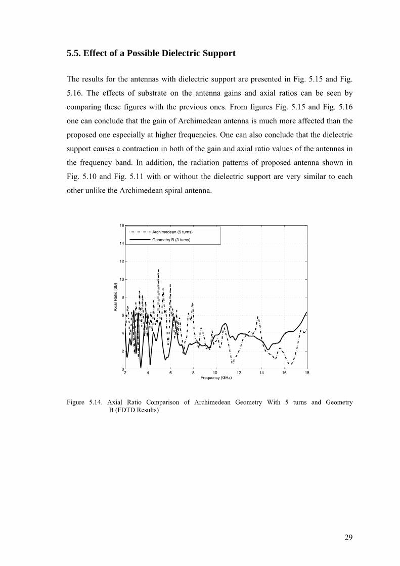
5.5. Effect of a Possible Dielectric Support The results for the antennas with dielectric support are presented in Fig. 5.15 and Fig.

5.16. The effects of substrate on the antenna gains and axial ratios can be seen by

comparing these figures with the previous ones. From figures Fig. 5.15 and Fig. 5.16

one can conclude that the gain of Archimedean antenna is much more affected than the

proposed one especially at higher frequencies. One can also conclude that the dielectric

support causes a contraction in both of the gain and axial ratio values of the antennas in

the frequency band. In addition, the radiation patterns of proposed antenna shown in

Fig. 5.10 and Fig. 5.11 with or without the dielectric support are very similar to each

other unlike the Archimedean spiral antenna.

2 4 6 8 10 12 14 16 180

2

4

6

8

10

12

14

16

Frequency (GHz)

Axi

al R

atio

(dB

)

Archimedean (5 turns)

Geometry B (3 turns)

Figure 5.14. Axial Ratio Comparison of Archimedean Geometry With 5 turns and Geometry B (FDTD Results)

30

2 4 6 8 10 12 14 16 18−2

−1

0

1

2

3

4

5

6

7

8

Frequency (GHz)

Gai

n (d

B)

ArchimedeanGeometry B

Figure 5.15. Gain Comparison of Archimedean and Geometry B on a Dielectric Substrate (FDTD Results)

Figure 5.16. Axial ratio Comparison of Archimedean and Geometry B on a Dielectric Substrate (FDTD Results)

31

2 4 6 8 10 12 14 16 18−2

−1

0

1

2

3

4

5

6

7

8

Frequency (GHz)

Gai

n (d

B)

Archimedean (5 turns)Geometry B (3 turns)

Figure 5.17. Gain Comparison of Archimedean with 5 Turns and Geometry B on a Dielectric Substrate (FDTD Results)

2 4 6 8 10 12 14 16 180

2

4

6

8

10

12

14

16

Frequency (GHz)

Axi

al R

atio

(dB

)

Geometry B (3 turns)Archimedean (5 turns)

Figure 5.18. Axial ratio Comparison of Archimedean with 5 Turns and Geometry B on a Dielectric Substrate (FDTD results)

32

Figure 5.19 Gain Comparison of Geometry C and Geometry D (FDTD results)

Figure 5.20 Axial ratio Comparison of Geometry C and Geometry D (FDTD results)

5.6. Measurement Procedure and Results

Lastly a larger two turn (exactly 781+ ) slot version of Geometry B and C are

realized on an FR-4 substrate with 1 mm thickness. Antennas were realized as slot

structures in order to feed antenna simpler. Antenna geometries are scaled to larger

dimensions due to difficulties of measurements in high frequencies. Realized antennas

33

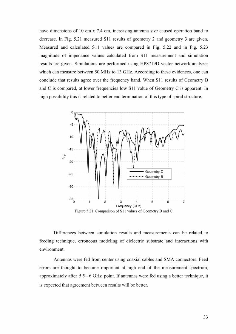
have dimensions of 10 cm x 7.4 cm, increasing antenna size caused operation band to

decrease. In Fig. 5.21 measured S11 results of geometry 2 and geometry 3 are given.

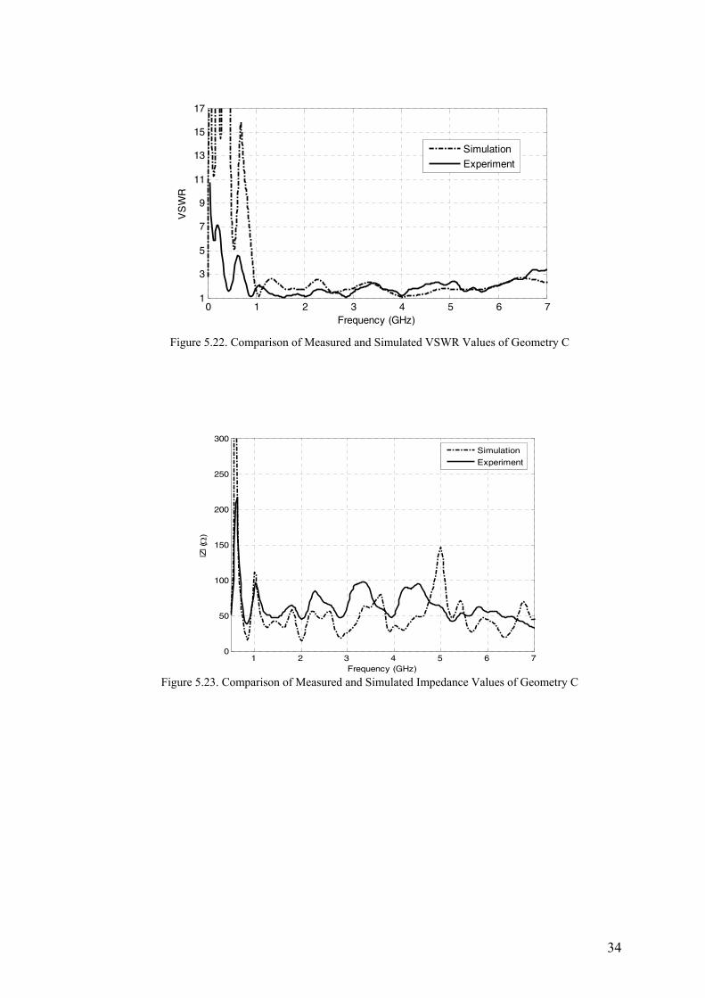
Measured and calculated S11 values are compared in Fig. 5.22 and in Fig. 5.23

magnitude of impedance values calculated from S11 measurement and simulation

results are given. Simulations are performed using HP8719D vector network analyzer

which can measure between 50 MHz to 13 GHz. According to these evidences, one can

conclude that results agree over the frequency band. When S11 results of Geometry B

and C is compared, at lower frequencies low S11 value of Geometry C is apparent. In

high possibility this is related to better end termination of this type of spiral structure.

0 1 2 3 4 5 6 7 -35

-30

-25

-20

-15

-10

-5

0

Frequency (GHz)

|S11

|

Geometry C

Geometry B

Figure 5.21. Comparison of S11 values of Geometry B and C

Differences between simulation results and measurements can be related to

feeding technique, erroneous modeling of dielectric substrate and interactions with

environment.

Antennas were fed from center using coaxial cables and SMA connectors. Feed

errors are thought to become important at high end of the measurement spectrum,

approximately after 5.5 6 GHz− point. If antennas were fed using a better technique, it

is expected that agreement between results will be better.

34

0 1 2 3 4 5 6 71

3

5

7

9

11

13

15

17

Frequency (GHz)

VS

WR

Simulation

Experiment

Figure 5.22. Comparison of Measured and Simulated VSWR Values of Geometry C

1 2 3 4 5 6 7 0

50

100

150

200

250

300

Frequency (GHz)

|Z| (Ω

)

Simulation

Experiment

Figure 5.23. Comparison of Measured and Simulated Impedance Values of Geometry C

35

CHAPTER 6

CONCLUSION

In this study novel type of rectangular spiral antennas are designed, analyzed

and examined. For numerical analysis two different methods, finite difference time

domain and method of moments are used and calculated results by these methods are

also compared with measurements. Proposed antennas generally show better

performance in terms of frequency independency of fundamental antenna parameters

when compared with the rectangular Archimedean geometry. Geometry B which can be

called hybrid logarithmic-Archimedean spiral antenna, generally performed better than

Geometry A which is expected to have better performance. Geometry C and D was also

show better performance than Archimedean geometry but they were not better than

Geometry B in terms of frequency dependency. However, Geometry C and D had

higher antenna gain values than the first two. The antenna parameters for the proposed

geometries are less dependent to the amount of turns, compared with Archimedean

spiral geometries. Therefore the proposed antennas can be used instead of square

Archimedean spiral geometries, especially if structure complexity is important.

The numerical and experimental results are also in a very good agreement. For

Geometry C, its S11 values are under -5dB in 0.7 GHz – 7 GHz band, and under -10 dB

in 0.85 GHz – 3.2 GHz band. Therefore this antenna has -5 dB impedance bandwidth of

1:10 and has -10 dB impedance bandwidth of 1:3.8. According to radiating ring theory,

this antenna should operate between 0.857 - 7.21 GHz which agrees with measurement

results. Examining measured geometry which has 781 amount of turns, one can conclude

that even using such a small number of turns for the spiral, very large bandwidths can

be obtained.

36

REFERENCES

Dyson, J.D. 1954. The Equiangular Spiral Antenna. IRE Transactions on Antennas and

Propagation. 7:181-188.

Kaiser, J.A. 1960. The Archimedean two-wire spiral antenna. IRE Transactions on

Antennas and Propagation. 8:312-323.

Curtis, W.L. 1960. Spiral antennas. IRE Transactions on Antennas and Propagation.

8:298-306.

Wang, J. J. H. and Tripp, V. K. 1991. Design of Multioctave Spiral-Mode Microstrip

Antennas. IEEE Transactions On Antennas And Propagation. 39:332-335

Kramer, B.A., Lee, M., Chen, C.C., and Volakis, J.L. 2005. Design and Performance of

an Ultrawide-Band Ceramic-Loaded Slot Spiral. IEEE Transactions On

Antennas And Propagation. 53:2193-2199.

Filipovic D.S., and Volakis J.L. 2002. Broadband Meanderline Slot Spiral Antenna.

IEE Proc-Microw. Antennas Propagat. 149:98-104.

Nurnberger M. W. and Volakis J. L. 2000. Extremely broadband slot spiral antennas

with shallow reflecting cavities. Electromagnetics. 20:357-376.

Iwasaki, T.A., Freundorfer, P., and Iizuka, K. 1994. A, unidirectional semicircular spiral

antenna for subsurface radars. IEEE Transactions on Electromagnetic

Compatibility. 36:1-6.

Bawer, Robert, and Wolfe, John. 1960. The Spiral Antenna. IRE International

Convention Record, New York, U.S.A. 1:84-95.

Rumsey, Victor. 1966. Frequency Independent Antennas. New York and London:

Academic Press.

Dyson, J.D., Bawer, R., Mayes, P.E. and Wolfe, J.I. 1961. A Note on the Difference

between Equiangular and Archimedes Spiral Antennas. IEEE Transactions on

Microwave Theory and Techniques. 9:203-205.

Kraus, John. and Marhefka, Ronald. 2002. Antennas. New York: McGraw-Hill.

Balanis, Constantine. 1997. Antenna Theory-Analysis and Design. New York: Wiley.

37

Brown, E. R., Lee, A. W. M., Navi, B.S. and Bjarnason, J.E., 2006. Characterization of

Planar Self-Complementary Square-Spiral Antenna in the THz Region.

Microwave and Optical Techology Letters 48: 524-528.

Poynting Software Ltd. SuperNEC 2.7 User’s Manual. www.supernec.com.

Remcom inc. XFDTD Bio-pro V6.2 User’s Manual. www.remcom.com.

Caswell E. D. 2001. Design and Analysis of Star Spiral with Application to Wideband

Array with Variable Element Sizes. Doctor of Philosophy Dissertation, Virginia

Polytechnic Institute and State University.

Gloutak R. T., Jr. and Alexopoulos N. G. 1997. Two-Arm Eccentric Spiral Antenna.

IEEE Transactions on Antennas and Propagation. 45: 723-730.

Ely J., Christodoulou C. and Shively D. 1995. Square Spiral Antennas for Wireless

Applications. IEEE NTC Conference, Orlando, FL. 229-232.

Sevgi L. and Cakir G. 2006. A Broadband Array of Archimedean Spiral Antennas for

Wireless Applications. Microwave and Optical Technology Letters. 48: 195-200.

Bell J.M. and Iskander M. F. 2004. A low-profile Archimedean spiral antenna using a

EBG ground plane. IEEE Antennas Wireless Propagat. Lett. 3: 223-226.

Nakano H., Ikeda M., Hitosugi K. and Yamauchi J. 2004. A spiral antenna sandwiched

by dielectric layers. IEEE Transactions on Antennas and Propagation. 52: 1417-

1423.

Nakano H., Yasui H., and Yamauchi J. 2002. Numerical analysis of two-arm spiral

antennas printed on a finite-size dielectric substrate. IEEE Transactions on

Antennas and Propagation. 50: 362-370.

H. Nakano, K. Nogami, S. Arai, H. Mimaki and J. Yamauchi. 1986. A spiral antenna

backed by a conducting plane reflector. IEEE Transactions on Antennas and

Propagation. 34: 791-796.

Penney C. W. and Luebbers R. J. 1994. Input impedance, radiation pattern and radar

cross section of spiral antennas using FDTD. IEEE Transactions on Antennas

and Propagation. 42: 1328-1332.