the monitoring of the spacecraft equipment thermal modes
TRANSCRIPT
The Monitoring of the Spacecraft Equipment Thermal Modes
A.Yu. Istratov
Moscow Institute of Electronics and
Mathematics
Higher School of Economics
Moscow, Russia
I.I. Khomenko
Moscow Institute of Electronics and
Mathematics
Higher School of Economics
Moscow, Russia
A.V. Pogodin
Department of ballistic and navigation
supply of near-Earth and moon
spacecraft
NPO Lavochkin
Moscow, Khimki
Abstract—In this paper the approach to the temperature
parameters forecasting to avoid overheating of the spacecraft
equipment at the end of the data transmission session is
considered. To determine temperature values at the indicated
times of the spacecraft components algorithms of historical data
processing are proposed. The software is provided. The
conducted experiments proved the ability to reveal anomaly
situations.
Keywords—Neural Network; Thermal Mode; Forecasting;
Spacecraft; Machine Learning
I. INTRODUCTION
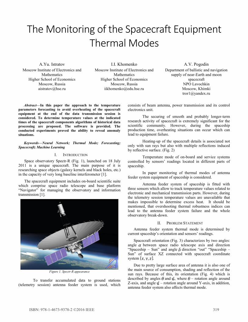
Space observatory Spectr-R (Fig. 1), launched on 18 July 2011 is a unique spacecraft. The main purpose of it is researching space objects (galaxy kernels and black holes, etc.) in the capacity of very long baseline interferometer [1].
The spacecraft equipment includes on-board scientific suite which comprise space radio telescope and base platform “Navigator” for managing the observatory and information transmission [1].
Figure 1. Spectr-R appearance
To transfer accumulated data to ground stations (telemetry session) antenna feeder system is used, which
consists of beam antenna, power transmission and its control electronics unit.
The securing of smooth and probably longer-term research activity of spacecraft is extremely significant for the scientific community. However, during the spaceship production time, overheating situations can occur which can lead to equipment failure.
Heating-up of the spacecraft details is associated not only with sun rays but also with multiple reflections induced by reflective surface. (Fig. 2)
Temperature mode of on-board and service systems controlled by sensors’ readings located in different parts of spaceship.
In paper monitoring of thermal modes of antenna feeder system equipment of spaceship is considered.
Antenna feeder system of spaceship is fitted with three sensors which allow to track temperature values related to electronic and mechanical transmission parts. However, during the telemetry session temperature values are unavailable that makes impossible to determine excess heat. It should be mentioned, that overshooting thermal robustness indices can lead to the antenna feeder system failure and the whole observatory break-down.
II. PROBLEM STATEMENT
Antenna feeder system thermal mode is determined by current spaceship’s orientation and sensors’ readings.
Spacecraft orientation (Fig. 3) characterizes by two angles: angle between space radio telescope axis and direction “Spaceship – Sun” and angle direction “out” “Spaceship – Sun” of surface XZ connected with spacecraft coordinate system .
Due to pretty large surface area of antenna it is also one of the main source of consumption, shading and reflection of the sun rays. Because of this, its orientation (Fig. 4) which is described by angles and , where – rotation angle around Z-axis, and angle – rotation angle around Y-axis, in addition, antenna feeder system also affects thermal mode.
ISBN: 978-1-4673-9378-2 ©2016 IEEE 319
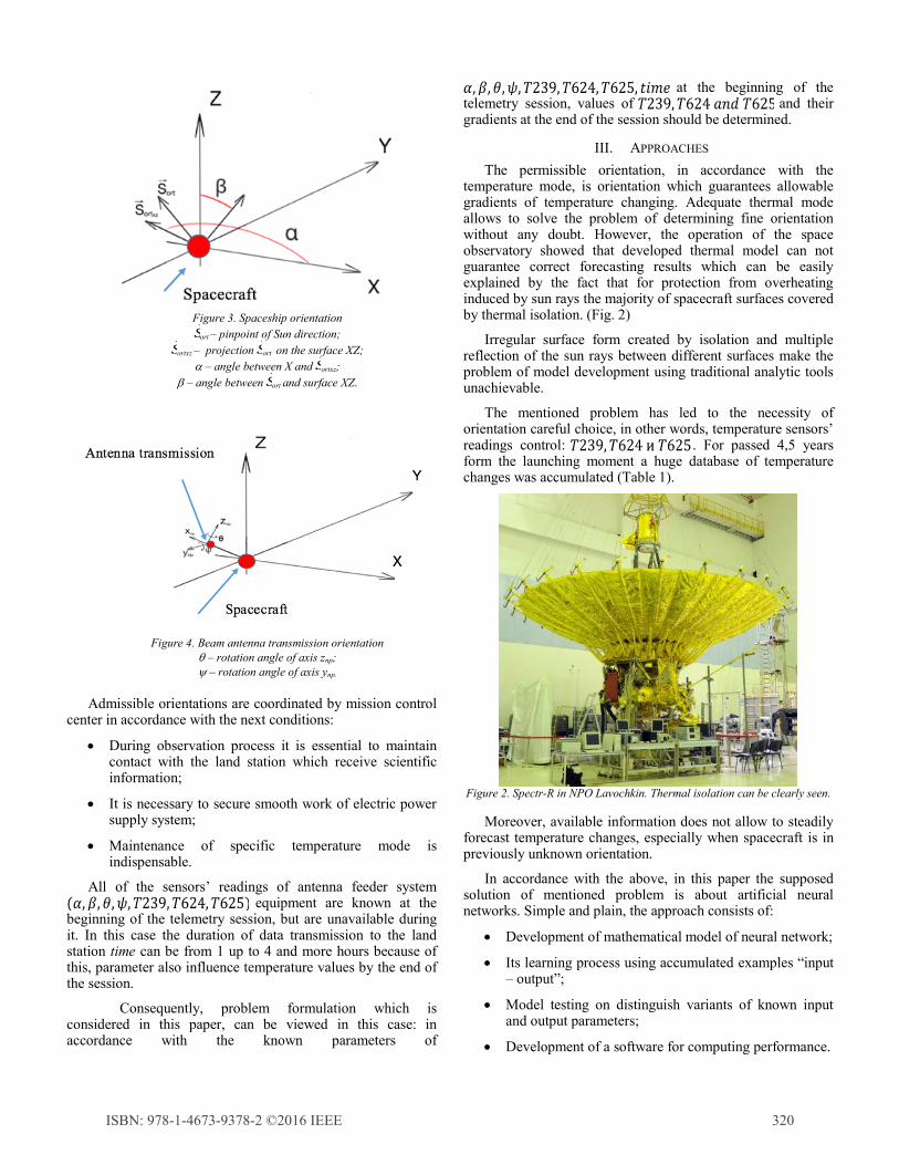
Figure 3. Spaceship orientation
ort – pinpoint of Sun direction;
ortxz – projection ort on the surface XZ;
– angle between X and ortxz;
– angle between ort and surface XZ.
Figure 4. Beam antenna transmission orientation
– rotation angle of axis zпр;
– rotation angle of axis yпр.
Admissible orientations are coordinated by mission control center in accordance with the next conditions:
During observation process it is essential to maintaincontact with the land station which receive scientificinformation;
It is necessary to secure smooth work of electric powersupply system;
Maintenance of specific temperature mode isindispensable.
All of the sensors’ readings of antenna feeder system equipment are known at the
beginning of the telemetry session, but are unavailable during it. In this case the duration of data transmission to the land station time can be from 1 up to 4 and more hours because of this, parameter also influence temperature values by the end of the session.
Consequently, problem formulation which is considered in this paper, can be viewed in this case: in accordance with the known parameters of
at the beginning of the telemetry session, values of and their gradients at the end of the session should be determined.
III. APPROACHES
The permissible orientation, in accordance with the temperature mode, is orientation which guarantees allowable gradients of temperature changing. Adequate thermal mode allows to solve the problem of determining fine orientation without any doubt. However, the operation of the space observatory showed that developed thermal model can not guarantee correct forecasting results which can be easily explained by the fact that for protection from overheating induced by sun rays the majority of spacecraft surfaces covered by thermal isolation. (Fig. 2)
Irregular surface form created by isolation and multiple reflection of the sun rays between different surfaces make the problem of model development using traditional analytic tools unachievable.
The mentioned problem has led to the necessity of orientation careful choice, in other words, temperature sensors’ readings control: . For passed 4,5 years form the launching moment a huge database of temperature changes was accumulated (Table 1).
Figure 2. Spectr-R in NPO Lavochkin. Thermal isolation can be clearly seen.
Moreover, available information does not allow to steadily forecast temperature changes, especially when spacecraft is in previously unknown orientation.
In accordance with the above, in this paper the supposed solution of mentioned problem is about artificial neural networks. Simple and plain, the approach consists of:
Development of mathematical model of neural network;
Its learning process using accumulated examples “input– output”;
Model testing on distinguish variants of known inputand output parameters;
Development of a software for computing performance.
ISBN: 978-1-4673-9378-2 ©2016 IEEE 320
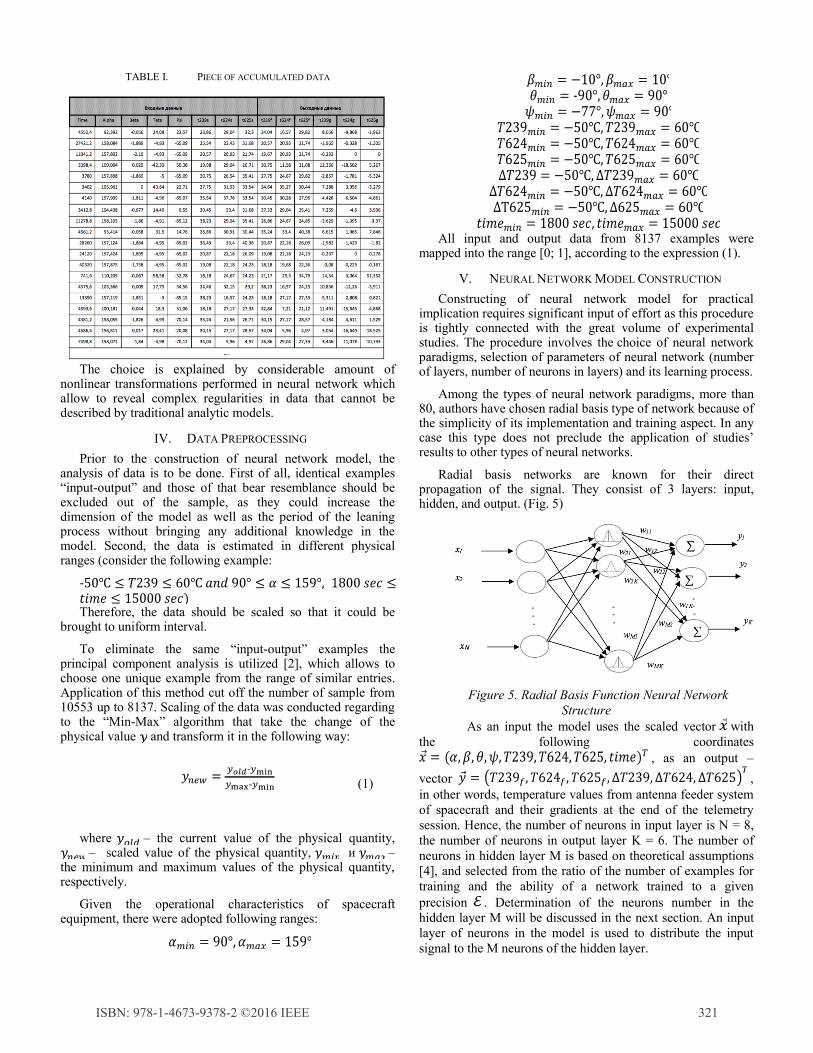
TABLE I. PIECE OF ACCUMULATED DATA
The choice is explained by considerable amount of nonlinear transformations performed in neural network which allow to reveal complex regularities in data that cannot be described by traditional analytic models.
IV. DATA PREPROCESSING
Prior to the construction of neural network model, the analysis of data is to be done. First of all, identical examples “input-output” and those of that bear resemblance should be excluded out of the sample, as they could increase the dimension of the model as well as the period of the leaning process without bringing any additional knowledge in the model. Second, the data is estimated in different physical ranges (consider the following example:
Therefore, the data should be scaled so that it could be brought to uniform interval.
To eliminate the same “input-output” examples the principal component analysis is utilized [2], which allows to choose one unique example from the range of similar entries. Application of this method cut off the number of sample from 10553 up to 8137. Scaling of the data was conducted regarding to the “Min-Max” algorithm that take the change of the physical value and transform it in the following way:
(1)
where – the current value of the physical quantity,– scaled value of the physical quantity, и –
the minimum and maximum values of the physical quantity, respectively.
Given the operational characteristics of spacecraft equipment, there were adopted following ranges:
All input and output data from 8137 examples were mapped into the range [0; 1], according to the expression (1).
V. NEURAL NETWORK MODEL CONSTRUCTION
Constructing of neural network model for practical implication requires significant input of effort as this procedure is tightly connected with the great volume of experimental studies. The procedure involves the choice of neural network paradigms, selection of parameters of neural network (number of layers, number of neurons in layers) and its learning process.
Among the types of neural network paradigms, more than 80, authors have chosen radial basis type of network because of the simplicity of its implementation and training aspect. In any case this type does not preclude the application of studies’ results to other types of neural networks.
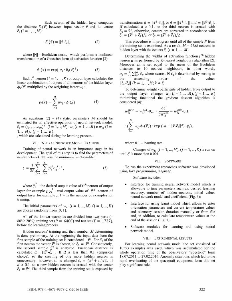
Radial basis networks are known for their direct propagation of the signal. They consist of 3 layers: input, hidden, and output. (Fig. 5)
Figure 5. Radial Basis Function Neural Network
Structure
As an input the model uses the scaled vector with
the following coordinates
, as an output –
vector ,
in other words, temperature values from antenna feeder system
of spacecraft and their gradients at the end of the telemetry
session. Hence, the number of neurons in input layer is N = 8,
the number of neurons in output layer K = 6. The number of
neurons in hidden layer M is based on theoretical assumptions
[4], and selected from the ratio of the number of examples for
training and the ability of a network trained to a given
precision . Determination of the neurons number in the
hidden layer M will be discussed in the next section. An input
layer of neurons in the model is used to distribute the input
signal to the M neurons of the hidden layer.
ISBN: 978-1-4673-9378-2 ©2016 IEEE 321
Each neuron of the hidden layer computes the distance between input vector and its centre
:
(2)
where – Euclidean norm, which performs a nonlineartransformation of a Gaussian form of activation function [3]:
(3)
Each jth neuron of output layer calculates the
linear combination of outputs of all neurons of the hidden layer multiplied by the weighting factor :
(4)
As equations (2) – (4) state, parameters M should be estimated for an effective operation of neural network model,
, which are calculated during the learning process.
VI. NEURAL NETWORK MODEL TRAINING
Training of neural network is an important stage in its development. The goal of this step is to find the parameters of neural network delivers the minimum functionality:
(5)
where – the desired output value of neuron of output
layer for example , – real output value of neuron of
output layer for example , P – is the number of examples for training.
The initial parameters of
are chosen randomly from [0; 1].
All of the known examples are divided into two parts (~ 80%: 20%): training set ( and test set ( , before the learning process.
Hidden neurons' training and their number M determining is done preliminary. At the beginning the input data from the first sample of the training set is considered – . For of the first neuron the vector is chosen, so . Consequently, the second sample is analyzed. Euclidean distance is calculated . If is less than 0.1 (empirical choice), so the creating of one more hidden neuron is unnecessary, however, is changed . If
, so a new hidden neuron is created with the center . The third sample from the training set is exposed by
transformations , or и, . If calculated , so the third neuron is created with
, otherwise, centers are corrected in accordance with , or .
This procedure is in progress until all of the sample P from the training set is examined. As a result, М = 5188 neurons in hidden layer with the centers .
Determining the widths of activation function hidden neuron is performed by K-nearest neighbours algorithm [2]. Moreover, is set equal to the mean of the Euclidean distances to 10 nearest neighbours, in other words,
, where nearest 10 is determined by sorting in
the ascending order of the values
To determine weight coefficients of hidden layer output to the output layer changes
minimizing functional the gradient descent algorithm is considered [4]:
where 0.1 – learning rate.
Changes of is run on
until is more than 0.001.
VII. SOFTWARE
To run the experiment researches software was developed using Java programming language.
Software includes:
Interface for training neural network model which isallowable to tune parameters such as: desired learningaccuracy, number of hidden neurons, initial valuesneural network model and coefficient. (Fig. 6);
Interface for using learnt model which allows to enterorientation parameters and current temperature valuesand telemetry session duration manually or from fileand, in addition, to calculate temperature values at theend of the session (Fig. 7);
Software modules for learning and using neuralnetwork model.
VIII. EXPIREMENTAL RESULTS
For learning neural network model the set consisted of 10553 examples was used, which was accumulated for the whole operation time of the observatory “Spectr-R” form 18.07.2011 to 27.02.2016. Anomaly situations which led to the rapid overheating of the spacecraft equipment form this set play significant role.
ISBN: 978-1-4673-9378-2 ©2016 IEEE 322
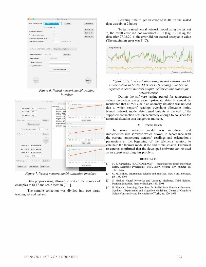
Figure 6. Neural network model training
interface
Figure 7. Neural network model utilization interface
Data preprocessing allowed to reduce the number of examples to 8137 and scale them in [0; 1].
The sample collection was divided into two parts: training set and test set.
Learning time to get an error of 0.001 on the scaled data was about 2 hours.
To test trained neural network model using the test set T, the result error did not overshoot 6 ˚С (Fig. 8). Using the data after 27.02.2016, the error did not exceed acceptable value (The maximum error was 8 ˚С).
Figure 8. Test set evaluation using neural network model.
Green colour indicates Т239 sensor's readings. Red curve
represents neural network output. Yellow colour stands for
network error. During the software testing period for temperature
values prediction using more up-to-date data. It should be mentioned that at 25.03.2016 an anomaly situation was noticed due to which sensors’ readings overshoot allowable limits. Neural network model determined outputs at the end of the supposed connection session accurately enough to consider the assumed situation as a dangerous moment.
IX. CONSLUSION
The neural network model was introduced and implemented into software which allows, in accordance with the current temperature sensors’ readings and orientation’s parameters at the beginning of the telemetry session, to calculate the thermal mode at the end of the session. Empirical researches confirmed that the developed software can be used as an expert regarding this problem.
REFERENCES
[1] N. S. Kardeshev, “RADIOASTRON” —radiotelescope much more than Earth. Scientific Programms, UFN, 2009, volume 179, number 11, 1191–1202
[2] C. M. Bishop. Information Science and Statistics. New York. Springer, pp. 738, 2006
[3] S. Haykin. Neural Networks and Learning Machines. Third Edition. Pearson Education, Prentice Hall, pp. 889, 2008
[4] E. Blanzieri. Learning Algorithms for Radial Basis Function Networks: Synthesis, Experiments and Cognitive Modelling. Center of Cognitive Science University and Polytechnic of Turin, pp. 120, 1998
Temperature,
Number of examples, units
ISBN: 978-1-4673-9378-2 ©2016 IEEE 323