the method of random groups kirk wolter

P1: OTE/SPH P2: OTE

SVNY318-Wolter December 13, 2006 19:54

CHAPTER 2

The Method of Random Groups

2.1. Introduction

The random group method of variance estimation amounts to selecting two ormore samples from the population, usually using the same sampling design foreach sample; constructing a separate estimate of the population parameter of in-terest from each sample and an estimate from the combination of all samples;and computing the sample variance among the several estimates. Historically,this was one of the first techniques developed to simplify variance estimation forcomplex sample surveys. It was introduced in jute acreage surveys in Bengalby Mahalanobis (1939, 1946), who called the various samples interpenetrat-ing samples. Deming (1956), the United Nations Subcommission on StatisticalSampling (1949), and others proposed the alternative term replicated samples.Hansen, Hurwitz, and Madow (1953) referred to the ultimate cluster techniquein multistage surveys and to the random group method in general survey appli-cations. Beginning in the 1990s, various writers have referred to the resamplingtechnique. All of these terms have been used in the literature by various authors,and all refer to the same basic method. We will employ the term random groupwhen referring to this general method of variance estimation.

There are two fundamental variations of the random group method. The firstcase is where the samples or random groups are mutually independent, while thesecond case arises when there is a dependency of some kind between the randomgroups. The case of independent samples is treated in Section 2.2. Although thisvariation of the method is not frequently employed in practice, there is exact theoryregarding the properties of the estimators whenever the samples are independent.In practical applications, the samples are often dependent in some sense, and exactstatistical theory for the estimators is generally not available. This case is discussedbeginning in Section 2.3.

21

P1: OTE/SPH P2: OTE


22 2. The Method of Random Groups

2.2. The Case of Independent Random Groups

Mutual independence of the various samples (or, more properly, of estimatorsderived from the samples) arises when one sample is replaced into the populationbefore selecting the next sample. To describe this in some detail, we assumethere exists a well-defined finite population and that it is desired to estimate someparameter θ of the population. We place no restrictions on the form of the parameterθ . It may be a linear statistic such as a population mean or total, or nonlinear suchas a ratio of totals or a regression or correlation coefficient.

The overall sampling scheme that is required may be described as follows:

(i) A sample, s1, is drawn from the finite population according to a well-definedsampling design (S , P ). No restrictions are placed on the design: it mayinvolve multiple frames, multiple stages, fixed or random sample sizes, doublesampling, stratification, equal or unequal selection probabilities, or with orwithout replacement selection, but the design is not restricted to these features.

(ii) Following the selection of the first sample, s1 is replaced into the population,and a second sample, s2, is drawn according to the same sampling design(S , P ).

(iii) This process is repeated until k ≥ 2 samples, s1, . . . , sk , are obtained, eachbeing selected according to the common sampling design and each beingreplaced before the selection of the next sample. We shall call these k samplesrandom groups.

In most applications of the random group method, there is a common estima-tion procedure and a common measurement process that is applied to each of thek random groups. Here, the terminology estimation procedure is used in a broadsense to include all of the steps in the processing of the survey data that occur afterthose data have been put in machine readable form. Included are such steps as theediting procedures, adjustments for nonresponse and other missing data, large ob-servation or outlier procedures, and the computation of the estimates themselves.In applying the random group method, there are no restrictions on any of thesesteps beyond those of good survey practice. The terminology measurement processis used in an equally broad sense to include all of the steps in the conduct of thesurvey up to and including the capture of the survey responses in machine readableform. This includes all of the data-collection work (whether it be by mail, tele-phone, or personal visit), callbacks for nonresponse, clerical screening and codingof the responses, and transcription of the data to machine readable form. There areno restrictions on any of these steps either, with one possible exception (seeAppendix D).1

1 In the study of measurement (or response) errors, it is assumed that the characteristic ofinterest Y cannot be observed. Rather, Y 0 is observed, where Y 0 is the characteristic Y plusan additive error e. If care is not taken, correlations between the various random groups canoccur because of correlations between the errors associated with units selected in differentrandom groups. An important example is where the errors are introduced by interviewers,

P1: OTE/SPH P2: OTE


2.2. The Case of Independent Random Groups 23

Application of the common measurement process and estimation procedureresults in k estimators of θ , which we shall denote by θα, α = 1, . . . , k. Then, themain theorem that describes the random group estimator of variance may be statedas follows.

Theorem 2.2.1. Let θ1, . . . , θk be uncorrelated random variables with commonexpectation E{θ1} = μ. Let ˆθ be defined by

ˆθ =k∑

α=1

θα/k.

Then E{ ˆθ} = μ and an unbiased estimator of Var{ ˆθ} is given by

v( ˆθ ) =k∑

α=1

(θα − ˆθ )2/k(k − 1). (2.2.1)

Proof. It is obvious that E{ ˆθ} = μ. The variance estimator v( ˆθ ) may be writtenas

v( ˆθ ) =[

k∑α=1

θ2α − k ˆ

θ2

] /k(k − 1).

Since the θα are uncorrelated, we have

E{v( ˆθ )} =[

k∑α=1

(Var{θα} + μ2) − k(Var{ ˆθ} + μ2)

] /k(k − 1)

= (k2 − k)Var{ ˆθ}/k(k − 1)

= Var{θα}. �

The statistic ˆθ may be used as the overall estimator of θ , while v( ˆθ ) is the randomgroup estimator of its variance Var{ ˆθ}.

In many survey applications, the parameter of interest θ is the same as theexpectation μ,

E{ ˆθ} = μ = θ, (2.2.1a)

or at least approximately so. In survey sampling it has been traditional to employdesign unbiased estimators, and this practice tends to guarantee (2.2.1a), at least incases where θα(α = 1, . . . , k) is a linear estimator and where θ is a linear function

and an interviewer’s assignment covers units selected from two or more random groups.To avoid such correlation, interviewer assignments should be arranged entirely within asingle random group. Error might also be introduced by other clerical operations, such asin coding survey responses on occupation, in which case clerical work assignments shouldbe nested within random groups.

P1: OTE/SPH P2: OTE



of the population parameter Y. When θ and θα are nonlinear, then μ and θ may beunequal because of a small technical bias arising from the nonlinear form.2

It is interesting to observe that Theorem 2.2.1 does not require that the variancesof the random variables θα be equal. Thus, the samples (or random groups) sα

could be generated by different sampling designs and the estimators θα could havedifferent functional forms, yet the theorem would remain valid so long as the θα areuncorrelated with common expectation μ. In spite of this additional generality ofTheorem 2.2.1, we will continue to assume the samples sα are each generated froma common sampling design and the estimators θα from a common measurementprocess and estimation procedure.

While Theorem 2.2.1 only requires that the random variables θα be uncorrelated,the procedure of replacing sample sα−1 prior to selecting sample sα tends to induceindependence among the θα . Thus, the method of sampling described by (i)–(iii)seems to more than satisfy the requirements of the theorem. However, the presenceof measurement errors, as noted earlier, can introduce a correlation between the θα

unless different sets of interviewers and different processing facilities are employedin the various samples. Certain nonresponse and poststratification adjustments mayalso introduce a correlation between the θα if they are not applied individuallywithin each sample. This topic is discussed further in Section 2.7.

Inferences about the parameter θ are usually based on normal theory or onStudent’s t theory. The central mathematical result is given in the following well-known theorem, which we state without proof.

Theorem 2.2.2. Let θ1, . . . , θk be independent and identically distributed normal(θ, σ 2) random variables. Then(i) the statistic

z = ( ˆθ − θ )/√

σ 2/k

is distributed as a normal (0, 1) random variable; and(ii) the statistic

t = ( ˆθ − θ )/

√v( ˆθ )

is distributed as Student’s t with k − 1 degrees of freedom. �

If the variance of ˆθ is essentially known without error or if k is very large, thena (1 − α) 100% confidence interval for θ is

( ˆθ − zα/2

√v( ˆθ ), ˆθ + zα/2

√v( ˆθ )),

where zα/2 is the upper α/2 percentage point of the N (0, 1) distribution.

2 In most simple examples, this bias is at most of order n−1, where n is the sample size.Such biases are usually unimportant in large samples.

P1: OTE/SPH P2: OTE



When the variance of ˆθ is not known or when k is not large, the confidence intervaltakes the form

( ˆθ − tk−1,α/2

√v( ˆθ ), ˆθ + tk−1,α/2

√v( ˆθ )),

where tk−1,α/2 is the upper α/2 percentage point of the tk−1 distribution.In like manner, statistical tests of hypotheses about θ may be based onTheorem 2.2.2.

The assumptions required in Theorem 2.2.2 are stronger than those inTheorem 2.2.1 and may not be strictly satisfied in sampling from finite pop-ulations. First, the random variables θα must now be independent and identi-cally distributed (θ, σ 2) random variables, whereas before they were only heldto be uncorrelated with common mean μ. These assumptions, as noted before,do not cause serious problems because the overall sampling scheme (i)–(iii) andthe common estimation procedure and measurement process tend to ensure thatthe more restrictive assumptions are satisfied. There may be concern about abias μ − θ �= 0 for nonlinear estimators, but such biases are usually unimpor-tant in the large samples encountered in modern complex sample surveys. Second,Theorem 2.2.2 assumes normality of the θα , and this is never satisfied exactlyin finite-population sampling. Asymptotic theory for survey sampling, however,suggests that the θα may be approximately normally distributed in large sam-ples. A discussion of some of the relevant asymptotic theory is presented inAppendix B.

Notwithstanding these failures of the stated assumptions, Theorem 2.2.2 hashistorically formed the basis for inference in complex sample surveys, largelybecause of the various asymptotic results.

Many of the important applications of the random group technique concernnonlinear estimators. In such applications, efficiency considerations may suggest

an estimator θ computed from the combination of all random groups, rather than ˆθ .

For certain linear estimators, θ and ˆθ are identical, whereas for nonlinear estimatorsthey are generally not identical. This point is discussed further in Section 2.8. The

difference between θ and ˆθ is illustrated in the following example.

Example 2.2.1. Suppose that it is desired to estimate the ratio

θ = Y/X,

where Y and X denote the population totals of two of the survey characteristics.Let Yα and Xα (α = 1, . . . , k) denote estimators of Y and X derived from the α-thrandom group. In practice, these are often linear estimators and unbiased for Yand X , respectively. Then,

θα = Yα/Xα,

ˆθ = (1/k)k∑

α=1

Yα/Xα,

P1: OTE/SPH P2: OTE



and

θ =

k∑α=1

Yα/k

k∑α=1

Xα/k

.

In general, ˆθ �= θ . �

There are two random group estimators of the variance of θ that are used inpractice. First, one may use

v1(θ ) =k∑

α=1

(θα − ˆθ )2/k(k − 1), (2.2.2)

which is the same as v( ˆθ ). Thus, v( ˆθ ) = v1(θ ) is used not only to estimate Var{ ˆθ},which it logically estimates, but also to estimate Var{θ}. However, straightforwardapplication of the Cauchy-Schwarz inequality gives

0 ≤[√

Var{ ˆθ} −√

Var{θ}]2

≤ Var{ ˆθ − θ}, (2.2.3)

and Var{ ˆθ − θ} is generally small relative to both Var{ ˆθ} and Var{θ}. In fact, using

Taylor series expansions (see Chapter 6), it is possible to show that Var{ ˆθ − θ} is

of smaller order than either Var{ ˆθ} or Var(θ}. Thus, the two variances are usuallyof similar magnitude and v1(θ ) should be a reasonable estimator of Var{θ}.

The second random group estimator is

v2(θ ) =k∑

α=1

(θα − θ )2/k(k − 1). (2.2.4)

When the estimator of θ is linear, then clearly ˆθ = θ and v1(θ ) = v2(θ ). Fornonlinear estimators, we have

k∑α=1

(θα − θ )2 =k∑

α=1

(θα − ˆθ )2 + k( ˆθ − θ )2. (2.2.5)

Thus,

v1(θ ) ≤ v2(θ )

and v2(θ ) will be preferred when a conservative estimate of variance is desired.

However, as observed before, the expectation of the squared difference ( ˆθ − θ )2

will be unimportant in many complex survey applications, and there should belittle difference between v1 and v2. If an important difference does occur between

v1 and v2 (or between ˆθ and θ ), then this could signal either a computational erroror a bias associated with small sample sizes.

P1: OTE/SPH P2: OTE



Little else can be said by way of recommending v1(θ ) or v2(θ ). Using second-order Taylor series expansions, Dippo (1981) has shown that the bias of v1 as anestimator of Var{θ} is less than or equal to the bias of v2. To the same order ofapproximation, Dippo shows that the variances of v1 and v2 are identical. Neitherof these results, however, has received any extensive empirical testing. And, ingeneral, we feel that it is an open question as to which of v1 or v2 is the moreaccurate estimator of the variance of θ .

Before considering the case of nonindependent random groups, we present a sim-ple, artificial example of the method of sample selection discussed in this section.

Example 2.2.2. Suppose that a sample of households is to be drawn using amultistage sampling design. Two random groups are desired. An areal frame exists,and the target population is divided into two strata (defined, say, on the basis ofgeography). Stratum I contains N1 clusters (or primary sampling units (PSU));stratum II consists of one PSU that is to be selected with certainty. Sample s1 isselected according to the following plan:

(i) Two PSUs are selected from stratum I using some πps sampling design. Fromeach selected PSU, an equal probability, single-start, systematic sample of m1

households is selected and enumerated.(ii) The certainty PSU is divided into well-defined units, say city blocks, with the

block size varying between 10 and 15 households. An unequal probabilitysystematic sample of m2 blocks is selected with probabilities proportional tothe block sizes. All households in selected blocks are enumerated.

After drawing sample s1 according to this plan, s1 is replaced and the secondrandom group, s2, is selected by independently repeating steps (i) and (ii).

Separate estimates, θ1, and θ2, of a population parameter of interest are computedfrom the two random groups. An overall estimator of the parameter and the randomgroup estimator of its variance are

ˆθ = (θ1 + θ2)/2

and

v( ˆθ ) = 1

2(1)

2∑α=1

(θα − ˆθ )2

= (θ1 − θ2)2/4,

respectively. �

The example nicely illustrates the simplifications that result from proper useof random groups. Had we not employed the random group method, varianceestimation would have been considerably more difficult, particularly for designsthat do not admit an unbiased estimator of variance; e.g., systematic samplingdesigns.

P1: OTE/SPH P2: OTE



2.3. Example: A Survey of AAA Motels3

We now illustrate the use of independent random groups with a real survey. Theexample is concerned with a survey of motel operators affiliated with the AmericanAutomobile Association (AAA). The purpose of the survey was to determinewhether the operators were in favor of instituting a system whereby motoristscould make reservations in advance of their arrival.

The survey frame was a file of cards maintained in the AAA’s central office. Itconsisted of 172 file drawers, with 64 cards per drawer. Each card represented oneof the following kinds of establishment:

a contract motel1 to 10 rooms

11 to 24 rooms25 rooms and over

a hotela restauranta special attractiona blank card.

The sampling unit was the card (or, equivalently, the establishment operator).The sampling design for the survey consisted of the following key features:

(1) Each of the 172 drawers was augmented by 6 blank cards, so that each drawernow contained 70 cards. This augmentation was based on 1) the prior beliefthat there were approximately 5000 contract motels in the population and 2)the desire to select about 700 of them into the overall sample. Thus, an overallsampling fraction of about one in 5000/700 = 7 was required.

(2) A sample of 172 cards was chosen by selecting one card at random from eachdrawer. Sampling was independent in different drawers.

(3) Nine additional samples were selected according to the procedure in Step 2.Each of the samples was selected after replacing the previous sample. Thus,estimators derived from the ten samples (or random groups) may be consideredto be independent.

(4) Eight hundred and fifty-four motels were drawn into the overall sample,and each was mailed a questionnaire. The 866 remaining units were notmembers of the domain for which estimates were desired (i.e., contract motels).Although the random groups were selected with replacement, no duplicateswere observed.

(5) At the end of 10 days, a second notice was sent to delinquent cases, and at theend of another week, a third notice. Every case that had not reported by theend of 24 days was declared a nonrespondent.

3 This example is from Deming (1960, Chapter 7). The permission of the author is gratefullyacknowledged.

P1: OTE/SPH P2: OTE


2.3. Example: A Survey of AAA Motels 29

Table 2.3.1. Number of Replies of Each Category to the Question “HowFrequently Do People Ask You to Make Reservations for Them?” After 24 Days

Random Ambiguous

Group Frequently Rarely Never Answer No Reply Yet Total

1 16 40 17 2 19 94

2 20 30 17 3 15 85

3 18 35 16 1 15 85

4 17 31 14 2 16 80

5 14 32 15 3 18 82

6 15 32 12 4 16 79

7 19 30 17 3 17 86

8 13 37 11 3 18 82

9 19 39 19 2 14 93

10 17 39 15 2 15 88

Total 168 345 153 25 163 854

Source: Table 3, Deming (1960, Chapter 7).

(6) Nonrespondents were then ordered by random group number, and from eachconsecutive group of three, one was selected at random. The selected nonre-spondents were enumerated via personal interview. In this sampling, nonre-spondents from the end of one random group were tied to those at the beginningof the next random group, thus abrogating, to a minor degree, the condition ofindependence of the random group estimators. This fact, however, is ignoredin the ensuing development of the example.

Table 2.3.1 gives the results to the question, “How frequently do people ask youto make reservations for them?” after 24 days. The results of the 1 in 3 subsampleof nonrespondents are contained in Table 2.3.2.

Estimates for the domain of contract motels may be computed by noting thatthe probability of a given sampling unit being included in any one of the randomgroups is 1/70, and the conditional probability of being included in the subsampleof nonrespondents is 1/3. Thus, for example, the estimated total number of contractmotels from the first random group is

X1 = 70172∑i=1

X1i

= 70(94)

= 6580,

where

X1i =⎧⎨⎩

1, if the i-th selected unit in the firstrandom group is a contract motel,

0, if not,

P1: OTE/SPH P2: OTE



Table 2.3.2. Results of Personal Interviews with the Subsample ofNonrespondents

Random Temporarily Closed

Group Frequently Rarely Never (vacation, sick, etc.) Total

1 1 2 2 1 6

2 1 2 1 1 5

3 2 2 0 1 5

4 2 1 2 0 5

5 1 3 1 2 7

6 2 2 0 1 5

7 1 3 1 1 6

8 1 2 1 2 6

9 2 2 1 0 5

10 1 2 0 2 5

Total 14 21 9 11 55

Source: Table 4, Deming (1960, Chapter 7).

and the estimated total over all random groups is

ˆX =10∑

α=1

Xα/10 = 5978.

Since the estimator is linear, X and ˆX are identical. The corresponding estimate ofvariance is

v( ˆX ) = 1

10(9)

10∑α=1

(Xα − ˆX )2 = 12,652.9.

Estimated totals for each of the categories of the question, “How frequentlydo people ask you to make reservations for them?” are given in Table 2.3.3. Forexample, the estimate from random group 1 of the total number of motels thatwould respond “frequently” is

Y1 = 70

(∑i∈r1

Y1i + 3∑i∈nr1

Y1i

)

= 70(16 + 3 · 1)

= 1330,

where∑

i∈r1and

∑i∈nr1

denote summations over the respondents and the subsam-ple of nonrespondents, respectively, in the first random group, and

Y1i =⎧⎨⎩

1, if the i-th selected unit in the first random group is acontract motel and reported “frequently,”

0, if not.

All of the estimates in Table 2.3.3 may be computed in this manner.

P1: OTE/SPH P2: OTE


2.3. Example: A Survey of AAA Motels 31

Table 2.3.3. Estimated Totals

Random Ambiguous Temporarily

Group Frequently Rarely Never Answer Closed

1 1330 3220 1610 140 210

2 1610 2520 1400 210 210

3 1680 2870 1120 70 210

4 1610 2380 1400 140 0

5 1190 2870 1260 210 420

6 1470 2660 840 280 210

7 1540 2730 1400 210 210

8 1120 3010 980 210 420

9 1750 3150 1540 140 0

10 1400 3150 1050 140 420

Parent

Sample 1470 2856 1260 175 231

Various nonlinear statistics may also be prepared from these data. The esti-mate from the first random group of the ratio of the “rarely” plus “never” to the“frequently” plus “rarely” plus “never” is

R1 = 3220 + 1610

1330 + 3220 + 1610= 0.784.

The estimate of this ratio over all random groups is

ˆR =10∑

α=1

Rα/10

= 0.737

with corresponding variance estimate

v( ˆR) = 1

10(9)

10∑α=1

(Rα − ˆR)2

= 0.0001139.

Since the ratio is a nonlinear statistic, we may use the alternative estimate

R = 2856 + 1260

1470 + 2856 + 1260= 0.737.

The two random group estimates of Var{R} are

v1(R) = v( ˆR)

= 0.0001139

P1: OTE/SPH P2: OTE



and

v2(R) = 1

10(9)

10∑α

(Rα − R)2 = 0.0001139.

Clearly, there is little difference between ˆR and R and between v1(R) and v2(R)for these data. A normal-theory confidence interval for the population ratio R isgiven by(

R ± 1.96

√v2(R)

)= (0.737 ± 1.96 ∗ 0.011) = (0.737 ± 0.021) .

2.4. The Case of Nonindependent Random Groups

In practical applications, survey samples are almost always selected as a wholeusing some form of sampling without replacement rather than by selecting a se-ries of independent random groups. Random groups are now formed followingsample selection by randomly dividing the parent sample into k groups. Estimatesare computed from each random group, and the variance is estimated using anexpression of the form of (2.2.1). The random group estimators θα are no longeruncorrelated because sampling is performed without replacement, and the result ofTheorem 2.2.1 is no longer strictly valid. The random group estimator now incurs abias. In the remainder of this section, we describe the formation of random groupsin some detail and then investigate the magnitude and sign of the bias for somesimple (but popular) examples.

2.4.1. The Formation of Random Groups

To ensure that the random group estimator of variance has acceptable statisticalproperties, the random groups must not be formed in a purely arbitrary fashion.Rather, the principal requirement is that they be formed so that each random grouphas essentially the same sampling design as the parent sample. This requirementcan be satisfied for most survey designs by adhering to the following rules:

(i) If a single-stage sample of size n is selected by either srs wor or pps worsampling, then the random groups should be formed by dividing the parentsample at random. This means that the first random group (RG) is obtainedby drawing a simple random sample without replacement (srs wor) of sizem = [n/k] from the parent sample, the second RG by drawing an srs wor ofsize m from the remaining n − m units in the parent sample, and so forth. Ifn/k is not an integer, i.e., n = km + q with 0 < q < k, then the q excess unitsmay be left out of the k random groups. An alternative method of handlingexcess units is to add one of the units to each of the first q RGs.

P1: OTE/SPH P2: OTE


2.4. The Case of Nonindependent Random Groups 33

(ii) If a single-start systematic sample of size n is selected with either equal orunequal probabilities, then the random groups should be formed by dividingthe parent sample systematically. This may be accomplished by assigning thefirst unit in the parent sample to random group 1, the second to random group2, and so forth in a modulo k fashion. Variance estimation for systematicsampling is discussed more fully in Chapter 8.

(iii) In multistage sampling, the random groups should be formed by dividing theultimate clusters, i.e., the aggregate of all elementary units selected from thesame primary sampling unit (PSU), into k groups. That is, all second, third,and successive stage units selected from the PSU must be treated as a singleunit when forming RGs. The actual division of the ultimate clusters intorandom groups is made according to either rule (i) or (ii), depending uponthe nature of the first-stage sampling design. If this design is either srs woror pps wor, then rule (i) should be used, whereas for systematic samplingdesigns rule (ii) should be used. Particular care is required when applyingthe ultimate cluster principle to so-called self-representing PSUs, whereterminology may cause considerable confusion.4 From the point of view ofvariance estimation, a self-representing PSU should be considered a separatestratum, and the units used at the first stage of subsampling are the basis forthe formation of random groups.

(iv) In stratified sampling, two options are available. First, if we wish to estimatethe variance within a given stratum, then we invoke either rule (i), (ii), or(iii) depending upon the nature of the within stratum sampling design. Forexample, rule (iii) is employed if a multistage design is used within thestratum. Second, if we wish to estimate the total variance across all strata,then each random group must itself be a stratified sample comprised of unitsfrom each stratum. In this case, the first RG is obtained by drawing an srswor of size mh = nh/k from the parent sample nh in the h-th stratum, forh = 1, . . . , L . The second RG is obtained in the same fashion by selectingfrom the remaining nh − mh units in the h-th stratum. The remaining RGsare formed in like manner. If excess observations remain in any of thestrata, i.e., nh = kmh + qh , they may be left out of the k random groupsor added, one each, to the first qh RGs. If the parent sample is selectedsystematically within strata, then the random groups must also be formed ina systematic fashion. In other words, each random group must be comprisedof a systematic subsample from the parent sample in each stratum.

(v) If an estimator is to be constructed for some double sampling scheme, such asdouble sampling for stratification or double sampling for the ratio estimator(see Cochran (1977, Chapter 12)), then the n′ sampling units selected into theinitial sample should be divided into the k random groups. The division shouldbe made randomly for srs wor and pps wor designs and systematically forsystematic sampling designs. When n′ is not an integer multiple of k, either ofthe procedures given in rule (i) for dealing with excess units may be used. The

4 A self-representing PSU is a PSU selected with probability one.

P1: OTE/SPH P2: OTE



second-phase sample, say of size n, is divided into random groups accordingto the division of the initial sample. In other words, a given selected unit i isassigned the same random group number as it was assigned in the initial sam-ple. This procedure is used when both initial and second-phase samples areselected in advance of the formation of random groups. Alternatively, in someapplications it may be possible to form the random groups after selection ofthe initial sample but before selection of the second-phase sample. In this case,the sample n′ is divided into the k random groups and the second-phase sam-ple is obtained by independently drawing m = n/k units from each randomgroup.

These rules, or combinations thereof, should cover many of the popular samplingdesigns used in modern large-scale sample surveys. The rules will, of course, haveto be used in combination with one another in many situations. An illustration iswhere a multistage sample is selected within each of L ≥ 2 strata. For this case,rules (iii) and (iv) must be used in combination. The ultimate clusters are thebasis for the formation of random groups, and each random group is composed ofultimate clusters from each stratum. Another example is where a double samplingscheme for the ratio estimator is used within each of L ≥ 2 strata. For this case,rules (iv) and (v) are used together. Some exotic sampling designs may not becovered by any combination of the rules. In such cases, the reader should attemptto form the random groups by adhering to the principal requirement that eachgroup has essentially the same design as the parent sample.

2.4.2. A General Estimation Procedure

In general, the estimation methodology for a population parameter θ is the sameas in the case of independent random groups (see Section 2.2). We let θ denote theestimator of θ obtained from the parent sample, θα the estimator obtained from

the α-th RG, and ˆθ = ∑kα=1 θα/k. The random group estimator of Var{ ˆθ} is then

given by

v( ˆθ ) = 1

k(k − 1)

k∑α=1

(θα − ˆθ )2, (2.4.1)

which is identical to (2.2.1). We estimate the variance of θ by either

v1(θ ) = v( ˆθ ) (2.4.2)

or

v2(θ ) = 1

k(k − 1)

k∑α=1

(θα − θ )2, (2.4.3)

which are identical to (2.2.2) and (2.2.4). When a conservative estimator of Var{θ}is sought, v2(θ ) is preferred to v1{θ}. The estimators θα should be prepared by

P1: OTE/SPH P2: OTE



application of a common measurement process and estimation procedure to eachrandom group. This process was described in detail in Section 2.2.

Because the random group estimators are not independent, v( ˆθ ) is not an unbi-

ased estimator of the variance of ˆθ . The following theorem describes some of theproperties of v( ˆθ ).

Theorem 2.4.1. Let θα be defined as above and let μα = E{θα}, where μα is notnecessarily equal to θ . Then,

E{ ˆθ} =k∑

α=1

μα/k(say)= μ,

and the expectation of the random group estimator of Var{ ˆθ} is given by

E{v( ˆθ )} = Var{ ˆθ} + 1

k(k − 1)

k∑α=1

(μα − μ)2

− 2k∑

α=1

k∑β>α

Cov{θα, θβ}/{k(k − 1)}.

Further, if each RG is the same size, then

μα = μ(α = 1, . . . , k),

E{ ˆθ} = μ,

and

E{v( ˆθ )} = Var{ ˆθ} − Cov{θ1, θ2}.

Proof. It is obvious that

E{ ˆθ} = μ.

The random group estimator of variance may be reexpressed as

v( ˆθ ) = ˆθ2 − 2k∑α

k∑β>α

θαθβ/k(k − 1).

The conclusion follows because

E{ ˆθ2} = Var{ ˆθ} + μ2

and

E{θαθβ} = Cov{θα, θβ} + μαμβ. �

Theorem 2.4.1 displays the bias inv( ˆθ ) as an estimator of Var{ ˆθ}. For large popu-lations and small sampling fractions, however, 2

∑kα

∑kβ>αCov{θα, θβ}/{k(k − 1)}

P1: OTE/SPH P2: OTE



will tend to be relatively small and negative. The quantity

1

k(k − 1)

k∑α=1

(μα − μ)2

will tend to be relatively small when μα = μ(α = 1, . . . , k). Thus, the bias of v( ˆθ )will be unimportant in many large-scale surveys and tend to be slightly positive.

When the estimator θ is linear, various special results and estimators are avail-able. This topic is treated in Subsections 2.4.3 and 2.4.4.

When the estimator θ is nonlinear, little else is known regarding the exactbias properties of (2.4.1), (2.4.2), or (2.4.3). Some empirical investigations of thevariance estimators have been encouraging in the sense that their bias is oftenfound to be unimportant. See Frankel (1971b) for one of the largest such studiesto date. The evidence as of this writing suggests that the bias of the random groupestimator of variance is often small and decreases as the size of the groups increase(or equivalently as the number of groups decreases). This result occurs becausethe variability among the θα is close to the variability in θ when the sample sizeinvolved in θα is close to that involved in θ . See Dippo and Wolter (1984) for adiscussion of this evidence.

It is possible to approximate the bias properties of the variance estimatorsby working with a linear approximation to θ (see Chapter 6) and then apply-ing known results for linear estimators. Such approximations generally suggestthat the bias is unimportant in the context of large samples with small sam-pling fractions. See Dippo (1981) for discussion of second-order approxima-tions.

2.4.3. Linear Estimators with Random Sampling of Elementary Units

In this subsection, we show how the general estimation procedure applies to a rathersimple estimator and sampling design. Specifically, we consider the problem ofvariance estimation for linear estimators where the parent sample is selected inL ≥ 1 strata. Within the h-th stratum, we assume that a simple random samplewithout replacement (srs wor) of nh elementary units is selected. Without essentialloss of generality, the ensuing development will be given for the case of estimatingthe population mean θ = Y .

The standard unbiased estimator of θ is given by

θ = yst =L∑

h=1

Wh yh,

where Wh = Nh/N , yh = ∑nhj=1 yhj/nh, Nh denotes the number of units in the

h-th stratum and N = ∑Lh=1 Nh . If nh is an integer multiple of k (i.e., nh = kmh)

for h = 1, . . . , L , then we form the k random groups as described by rule (iv) of

P1: OTE/SPH P2: OTE



Subsection 2.4.1 and the estimator of θ from the α-th RG is

θα = yst,α =L∑

h=1

Wh yh,α, (2.4.4)

where yh,α is the sample mean of the mh units in stratum h that were selected into theα-th RG. Because the estimator θ is linear and since nh = kmh for h = 1, . . . , L ,

it is clear that θ = ˆθ .The random group estimator of the variance Var{θ} is

v(θ ) = 1

k(k − 1)

k∑α=1

(yst,α − yst)2,

where it is clear that (2.4.1), (2.4.2), and (2.4.3) are identical in this case.

Theorem 2.4.2. When nh = kmh for h = 1, . . . , L, the expectation of the randomgroup estimator of Var{yst} is given by

E{v(θ )} =L∑

h=1

W 2h S2

h/nh,

where

S2h = 1

Nh − 1

Nh∑j=1

(Yhj − Yh)2.

Proof. By definition,

E{y2st,α} = Var{yst,α} + E2{yst,α}

=L∑

h=1

W 2h

(1

mh− 1

Nh

)S2

h + Y 2

and

E{y2st} = Var{yst} + E2{yst}

=L∑

h=1

W 2h

(1

nh− 1

Nh

)S2

h + Y 2.

The result follows by writing

v(θ ) = 1

k(k − 1)

(k∑

α=1

y2st,α − k y2

st

). �

The reader will recall that

Var{θ} =L∑

h=1

W 2h (1 − fh)S2

h/nh,

P1: OTE/SPH P2: OTE



where fh = nh/Nh is the sampling fraction. Thus, Theorem 2.4.2 shows that v(θ )is essentially unbiased whenever the sampling fractions fh are negligible. If someof the fh are not negligible, then v(θ ) is conservative in the sense that it will tendto overestimate Var{θ}.

If some of the sampling fractions fh are important, then they may be includedin the variance computations by working with

W ∗h = Wh

√1 − fh

in place of Wh . Under this procedure, we define the random group estimators by

θ∗α = yst +

L∑h=1

W ∗h (yh,α − yh), (2.4.5)

ˆθ∗ = 1

k

k∑α=1

θ∗α ,

and

v( ˆθ∗) = 1

k(k − 1)

k∑α=1

(θ∗α − ˆθ∗)2.

It is clear that

ˆθ∗ = θ = yst.

Corollary 2.4.1. Let v( ˆθ∗) be defined as v(θ ) with ˆθ∗α in place of θα . Then, given

the conditions of Theorem 2.4.2,

E{v( ˆθ∗)} =L∑

h=1

W ∗2h S2

h/nh

= Var{θ}. �

This corollary shows that an unbiased estimator of variance, including thefinite population corrections, can be achieved by exchanging the weights W ∗

h forWh .

Next, we consider the general case where the stratum sample sizes are notinteger multiples of the number of random groups. Assume nh = kmh + qh forh = 1, . . . ., L , with 0 ≤ qh < k. A straightforward procedure for estimating thevariance of θ = yst is to leave the qh excess observations out of the k randomgroups. The random group estimators are defined as before, but now

ˆθ =k∑

α=1

yst,α/k �= θ

because the excess observations are in θ but not in ˆθ . The expectation of therandom group estimator v( ˆθ ) is described by Theorem 2.4.2, where the nh in thedenominator is replaced by nh − qh = kmh .

P1: OTE/SPH P2: OTE



Corollary 2.4.2. Let v(θ ) be defined as in Theorem 2.4.2 with qh excess observa-tions omitted from the k random groups. Then,

E{v(θ )} =L∑

h=1

W 2h S2

h/kmh . �

The reader will immediately observe that v(θ ) tends to overestimate Var{θ},not only due to possibly nonnegligible fh but also because kmh ≤ nh . As before,if some of the fh are important, they may be accounted for by working with θ∗

α

instead of θα . If both the fh and the qh are important, they may be accounted forby replacing Wh by

W′′h = Wh

√(1 − fh)

kmh

nh

and by defining

θ′′α = yst +

L∑h=1

W′′h

(yh,α − 1

k

k∑β=1

yh,β

).

Then ˆθ′′ = θ and v( ˆθ

′′) is an unbiased estimator of Var{θ}.

An alternative procedure, whose main appeal is that it does not omit observa-tions, is to form qh random groups of size mh + 1 and k − qh of size mh . Letting

ah,α =

⎧⎪⎪⎨⎪⎪⎩

k(mh + 1)/nh, if the α-th RG contains mh + 1units from the h-th stratum,

kmh/nh, if the α-th RG contains mh unitsfrom the h-th stratum,

we define the α-th random group estimator by

θα =L∑

h=1

Whah,α yh,α.

It is important to note that

E{θα} =L∑

h=1

Whah,αYh

�= Y . (2.4.6)

However, because

˜θ =k∑

α=1

θα/k = yst = θ

P1: OTE/SPH P2: OTE



and E{θ} = θ, ˜θ is an unbiased estimator of θ even though the individual θα arenot unbiased. The random group estimator of Var{θ} is now given by

v( ˜θ ) = 1

k(k − 1)

k∑α=1

( θα − ˜θ )2

= 1

k(k − 1)

k∑α=1

( θα − θ )2. (2.4.7)

Theorem 2.4.3. When nh = kmh + qh for h = 1, . . . , L, the expectation of therandom group estimator v( ˜θ ) is given by

E{v( ˜θ )} = Var{yst} + 1

k(k − 1)

k∑α=1

(E{ θα} − θ )2

− 2k∑

α=1

k∑β>α

[h∑

h=1

W 2h ah,αah,β(−S2

h/Nh)

]/k(k − 1). (2.4.8)

Proof. Follows directly from Theorem 2.4.1 by noting that

Cov{ θα, θβ} =h∑

h=1

W 2h ah,αah,β(−S2

h/Nh)

whenever α �= β. �

The reader will observe that v( ˜θ ) is a biased estimator of Var{yst}, with the biasbeing given by the second and third terms on the right-hand side of (2.4.8). Whenthe fh’s are negligible, the contribution of the third term will be unimportant. Thecontribution of the second term will be unimportant whenever

E{ θα} =h∑

h=1

Whah,αYh = Y

for α = 1, . . . , k. Thus, in many surveys the bias of the random group estimatorv( ˜θ ) will be unimportant.

It is an open question as to whether the estimator v( ˜θ ) has better or worsestatistical properties than the estimator obtained by leaving the excess observationsout of the random groups.

2.4.4. Linear Estimators with Clustered Samples

In the last subsection, we discussed the simple situation where an srs wor ofelementary units is selected within each of L strata. We now turn to the casewhere a sample of n clusters (or PSUs) is selected and possibly several stagesof subsampling occur independently within the selected PSUs. To simplify thepresentation, we initially discuss the case of L = 1 stratum. The reader will be

P1: OTE/SPH P2: OTE



able to connect the results of Subsection 2.4.3 with the results of this subsectionto handle cluster sampling within L ≥ 2 strata. We continue to discuss linearestimators, only now we focus our attention on estimators of the population totalθ = Y .

Let N denote the number of PSUs in the population, Yi the population total in thei-th PSU, and Yi the estimator of Yi due to subsampling at the second and successivestages. The method of subsampling is left unspecified, but, for example, it mayinvolve systematic sampling or other sampling designs that ordinarily do not admitan unbiased estimator of variance. We assume that n PSUs are selected accordingto some πps scheme, so that the i-th unit is included in the sample with probability

πi = npi ,

where 0 < npi < 1,∑N

i=1 pi = 1, and pi is proportional to some measure of sizeXi . The reader will observe that srs wor sampling at the first stage is simply aspecial case of this sampling framework, with πi = n/N .

We consider estimators of the population total of the form

θ =n∑

i=1

Yi/πi =n∑

i=1

Yi/npi .5

The most common member of this class of estimators is

θ =n∑

i=1

ri∑j=1

wi j yi j ,

where i indexes the PSU, j indexes the complete interview within the PSU, ri isthe number of complete interviews within the PSU, and wi j denotes the weightcorresponding to the (i, j)-th respondent. See Section 1.6 for a discussion of caseweights.

After forming k = n/m (m an integer) random groups, the α-th random groupestimator is given by

θα =m∑

i=1

Yi/mpi ,

where the sum is taken over all PSUs selected into the α-th RG.The weighted version of this estimator is

θα =n∑

i=1

ri∑j=1

wαi j yi j ,

where the replicate weights are defined by

wαi j = wi jn

m, if i is a member of the random group,

5 The material presented here extends easily to estimators of the more general form θ =∑Ni=1 ais Yi , where the ais are defined in advance for each sample s and satisfy E{ais} = 1.

See Durbin (1953) and Raj (1966) for discussions of unbiased variance estimation for suchestimators.

P1: OTE/SPH P2: OTE



= 0, otherwise.

Because θ is linear in the Yi , it is clear that θ = ˆθ = ∑kα=1 θα/k. We define the

RG estimator of Var{θ} by

v(θ ) = 1

k(k − 1)

k∑α=1

( θα − θ )2. (2.4.9)

Some of the properties of v(θ ) are given in the following theorems.

Theorem 2.4.4. Let vk(θ ) be the estimator defined in (2.4.9) based on k randomgroups, and let n = km (m an integer). Then,

(i) E2{vk(θ )} = vn(θ ),(ii) Var{vk(θ )} ≥ Var{vn(θ )},

where E2 denotes the conditional expectation over all possible choices of k randomgroups for a given parent sample.

Proof. Part (i) follows immediately from Theorem 2.4.2 by letting L = 1. Part(ii) follows from part (i) since

Var{vk(θ )} = Var{E2{vk(θ )}} + E{Var2{vk(θ )}}≥ Var{E2{vk(θ )}}. �

Theorem 2.4.4 shows that vk(θ ) has the same expectation regardless of thevalue of k, so long as n is an integer multiple of k. However, the choice k = nminimizes the variance of the RG estimator. The reader will recall that vn(θ ) isthe standard unbiased estimator of the variance given pps wr sampling at the firststage.

Theorem 2.4.5. Let vk(θ ) be the estimator defined in (2.4.9) based on k randomgroups and let

Yi = E{Yi |i},σ 2

2i = Var{Yi |i},and n = km (m an integer). Then, the expectation of vk(θ ) is given by

E{vk(θ )} = E

⎧⎨⎩ 1

n(n − 1)

n∑i=1

(Yi/pi −

n∑j=1

Y j/np j

)2⎫⎬⎭ +

N∑i=1

σ 22i/npi .

(2.4.10)

Proof. The result follows from Theorem 2.4.4 and the fact that

vn(θ ) = 1

n(n − 1)

(n∑

i=1

Y2

i

p2i

− nY 2

)

P1: OTE/SPH P2: OTE



and that

E{Y 2i |i} = Y 2

i + σ 22i . �

Remarkably, (2.4.10) shows that the RG estimator completely includes thewithin component of variance since, the reader will recall,

Var{θ} = Var

{n∑

i=1

Yi/npi

}+

N∑i=1

σ 22i/npi . (2.4.11)

Thus, the bias in vk(θ ) arises only in the between component, i.e., the differencebetween the first terms on the right-hand side of (2.4.10) and (2.4.11). In surveyswhere the between component is a small portion of the total variance, we wouldanticipate that the bias in vk(θ ) would be unimportant. The bias is discussed furtherin Subsection 2.4.5, where it is related to the efficiency of πps sampling vis-a-vispps wr sampling.

Now let us see how these results apply in the case of srs wor sampling at thefirst stage. We continue to make no assumptions about the sampling designs atthe second and subsequent stages, except we do require that such subsampling beindependent from one PSU to another.

Corollary 2.4.3. Suppose the n PSUs are selected at random and without replace-ment. Then, the expectation of vk(θ ) is given by

E{vk(θ )} = N 2S2b/n + (N 2/n)σ 2

w, (2.4.12)

where

S2b = (N − 1)−1

N∑i=1

(Yi − N−1

N∑j=1

Y j

)2

and

σ 2w = N−1

N∑i=1

σ 22i . �

The true variance of θ given srs wor at the first stage is

Var{θ} = N 2(1 − n/N )S2b/n + (N 2/n)σ 2

w,

and thus vk(θ ) tends to overestimate the variance. Not surprisingly, the problemis with the finite-population correction (1 − n/N ). One may attempt to adjust forthe problem by working with the modified estimator (1 − n/N )vk(θ ), but thismodification is downward biased by the amount

Bias{(1 − n/N )vk(θ )} = −Nσ 2w.

Of course, when n/N is negligible, vk(θ ) is essentially unbiased.

P1: OTE/SPH P2: OTE



In the case of sampling within L ≥ 2 strata, similar results are available. Let theestimator be of the form

θ =L∑

h=1

Yh =L∑

h=1

nh∑i=1

Yhi

πhi,

where πhi = nh phi is the inclusion probability associated with the (h, i)-th PSU.Two random group methodologies were discussed for this problem in Subsection2.4.1. The first method works within strata, and the estimator of Var{Y} is of theform

v(θ ) =L∑

h=1

v(Yh),

v(Yh) = 1

k(k − 1)

k∑α=1

(Yhα − Yh)2, (2.4.13)

Yhα =mh∑i=1

Yhi

mh phi,

where the latter sum is over the mh units that were drawn into the α-th randomgroup within the h-th stratum. The second method works across strata, and theestimator is of the form

v(θ ) = 1

k(k − 1)

k∑α=1

(θα − θ )2,

θα =L∑

h=1

Yhα, (2.4.14)

Yhα =mh∑i=1

Yhi

mh phi,

where this latter sum is over the mh units from the h-th stratum that were assignedto the α-th random group. It is easy to show that both (2.4.13) and (2.4.14) havethe same expectation, namely

E{v(θ )} =L∑

h=1

E

⎧⎨⎩ 1

nh(nh − 1)

nh∑i=1

(Yhi

phi− 1

nh

nh∑j=1

Yhj

phj

)2⎫⎬⎭ +

L∑h=1

Nh∑i=1

σ 22hi

nh phi.

Since the true variance of Y is

Var{θ} =L∑

i=1

Var

{nh∑

i=1

Yhi

nh phi

}+

L∑h=1

Nh∑i=1

σ 22hi

nh phi,

we see once again that the random group estimator incurs a bias in the betweenPSU component of variance.

P1: OTE/SPH P2: OTE



In the case of stratified sampling, the weighted form of the estimator is

θ =L∑

h=1

nh∑i=1

rhi∑j=1

whi j yhi j ,

where there are rhi completed interviews in the (h, i)-th PSU and whi j is the weightcorresponding to the (h, i, j)-th interview. The corresponding RG estimator is

θα =L∑

h=1

nh∑i=1

rhi∑j=1

wαhi j yhi j ,

where the replicate weights are

wαhi j = whi jnh

mh, if the (h, i)-th PSU is in the α-th RG,

= 0, otherwise.

It may be possible to reduce the bias by making adjustments to the estimatoranalogous to those made in Subsection 2.4.3. Let

Var

{(nh∑

i=1

Yhi

nh phi

)wr

}

denote the between PSU variance given pps wr sampling within strata, and let

Var

{nh∑

i=1

Yhi

nh phi

}

denote the between variance given πps sampling. Suppose that it is possible toobtain a measure of the factor

Rh = nh

nh − 1

⎛⎜⎜⎜⎜⎝

{Var

(nh∑j=1

Yhi

nh phi

)wr

}

Var

{nh∑

i=1

Yhi

nh phi

} −Var

{nh∑

i=1

Yhi

nh phi

}

Var

{nh∑

i=1

Yhi

nh phi

}⎞⎟⎟⎟⎟⎠ ,

either from previous census data, computations on an auxiliary variable, or pro-fessional judgment. Then define the adjusted estimators

θ∗α = θ +

L∑h=1

A−1/2h (Yhα − Yh),

Ah = 1 + Rh .

It is clear that

ˆθ∗ =k∑

α=1

θ∗α/k = θ

P1: OTE/SPH P2: OTE



since the estimators are linear in the Yhi . If the Ah are known without error, thenthe usual random group estimator of variance

v( ˆθ∗) = 1

k(k − 1)

k∑α=1

(θ∗α − ˆθ∗)2

is unbiased for Var{θ}. The estimator v( ˆθ∗) will be biased to the extent that themeasures of Rh are erroneous. So long as the measures of Rh are reasonable,

however, the bias of v( ˆθ∗) should be reduced relative to that of v(θ ).The results of this subsection were developed given the assumption that

n (or nh) is an integer multiple of k. If n = km + q, with 0 < q < k, then eitherof the techniques discussed in Subsection 2.4.3 may be used to obtain the varianceestimator.

2.4.5. A General Result About Variance Estimation for WithoutReplacement Sampling

As was demonstrated in Theorem 2.4.4, the random group estimator tends toestimate the variance as if the sample were selected with replacement, eventhough it may in fact have been selected without replacement. The price wepay for this practice is a bias in the estimator of variance, although the bias isprobably not very important in modern large-scale surveys. An advantage ofthis method, in addition to the obvious computational advantages, is that thepotentially troublesome calculation of the joint inclusion probabilities πi j , presentin the Yates–Grundy estimator of variance, is avoided. In the case of srs wor,we can adjust for the bias by applying the usual finite-population correction. Forunequal probability sampling without replacement, there is no general correctionto the variance estimator that accounts for the without replacement feature. In thecase of multistage sampling, we know (see Theorem 2.4.5) that the bias occursonly in the between PSU component of variance.

This section is devoted to a general result that relates the bias of the randomgroup variance estimator to the efficiency of without replacement sampling. Weshall make repeated use of this result in future chapters. To simplify the discussion,we assume initially that a single-stage sample of size n is drawn from a finitepopulation of size N , where Yi is the value of the i-th unit in the populationand pi is the corresponding nonzero selection probability, possibly based uponsome auxiliary measure of size Xi . We shall consider two methods of drawingthe sample: (1) pps wr sampling and (2) an arbitrary πps scheme. The reader willrecall that a πps scheme is a without replacement sampling design with inclusionprobabilities πi = npi . Let

Yπps =n∑

i=1

yi/πi

denote the Horvitz–Thompson estimator of the population total given the πps

P1: OTE/SPH P2: OTE



scheme, where πi = npi , for i = 1, . . . , N , and let

Ywr = (1/n)n∑

i=1

yi/pi

denote the customary estimator of the population total Y given the pps wr scheme.Let Var{Yπps} and Var{Ywr} denote the variances of Yπps and Ywr, respectively.Further, let

v(Ywr) = {1/n(n − 1)}n∑

i=1

(yi/pi − Ywr)2

be the usual unbiased estimator of Var{Ywr}. Then we have the following.

Theorem 2.4.6. Suppose that we use the estimator v(Ywr) to estimate Var{Yπps}given the πps sampling design. Then, the bias of v(Ywr) is given by

Bias{v(Ywr)} = n

n − 1(Var{Ywr} − Var{Yπps}). (2.4.15)

Proof. The variances of Yπps and Ywr are

Var{Yπps} =N∑

i=1

πi (1 − πi )

(Yi

πi

)2

+ 2N∑

i=1

N∑j>i

(πi j − πiπ j )

(Yi

πi

) (Y j

π j

)

(2.4.16)

and

Var{Ywr} = 1

n

N∑i

pi

(Yi

pi− Y

)2

,

respectively. Thus

Var{Ywr} − Var{Yπps} = n − 1

nY 2 − 2

N∑i=1

N∑j>i

πi j

(Yi

πi

) (Y j

π j

).

The variance estimator may be expressed as

v(Ywr) =n∑

i=1

(yi

npi

)2

− 2

n − 1

n∑i=1

n∑j>i

(yi

npi

) (y j

np j

)

with expectation (given the πps sampling design)

E{v(Ywr)} =N∑

i=1

πi

(Yi

npi

)2

− 2

n − 1

N∑i=1

N∑j>i

πi j

(Yi

npi

) (Y j

np j

). (2.4.17)

Combining (2.4.16) and (2.4.17) gives

Bias{v(Ywr)} = Y 2 − 2n

n − 1

N∑i=1

N∑j>i

πi j

(Yi

πi

) (Y j

π j

),

from which the result follows immediately. �

P1: OTE/SPH P2: OTE



Theorem 2.4.6, originally due to Durbin (1953), implies that when we use thepps wr estimator v(Ywr) we tend to overestimate the variance of Yπps whenever thatvariance is smaller than the variance of Ywr given pps wr sampling. Conversely,when pps wr sampling is more efficient than the πps scheme, the estimator v(Ywr)tends to underestimate Var{Yπps}. Thus, we say that v(Ywr) is a conservative esti-mator of Var{Yπps} for the useful applications of πps sampling.

This result extends easily to the case of multistage sampling, and as before, thebias occurs only in the between PSU component of variance. To see this, considerestimators of the population total Y of the form

Yπps =n∑

i=1

Yi

πi,

Ywr = 1

n

n∑i=1

Yi

pi,

for πps sampling and pps wr sampling at the first stage, where Yi is an estimatorof the total in the i-th selected PSU due to sampling at the second and subsequentstages. Consider the pps wr estimator of variance

v(Ywr) = 1

n(n − 1)

n∑i=1

(Yi

pi− Ywr

)2

. (2.4.18)

Assuming that sampling at the second and subsequent stages is independent fromone PSU selection to the next, v(Ywr) is an unbiased estimator of Var{Ywr} givenpps wr sampling. When used for estimating the variance of Yπps given πps sam-pling, v(Ywr) incurs the bias

Bias{v(Ywr)} = Y 2 − 2n

n − 1

N∑i=1

N∑j>i

πi j

(Yi

πi

) (Y j

π j

)

= n

n − 1(Var{Ywr } − Var{Yπps}), (2.4.19)

where Yi is the total of the i-th PSU. See Durbin (1953). This result confirms thatthe bias occurs only in the between PSU component of variance. The bias will beunimportant in many practical applications, particularly those where the betweenvariance is a small fraction of the total variance.

Usage of (2.4.18) for estimating the variance of Yπps given πps sampling notonly avoids the troublesome calculation of the joint inclusion probabilities πi j ,but also avoids the computation of estimates of the components of variance due tosampling at the second and subsequent stages. This is a particularly nice featurebecause the sampling designs used at these stages often do not admit unbiasedestimators of the variance (e.g., systematic sampling).

The above results have important implications for the random group estimator ofvariance with n = km. By Theorem 2.4.4 we know that the random group estimator

P1: OTE/SPH P2: OTE



of Var{Yπps} given πps sampling and based upon k ≤ n/2 random groups, has thesame expectation as, but equal or larger variance than, the estimator v(Ywr). Infact, v(Ywr) is the random group estimator for the case (k, m) = (n, 1). Thus theexpressions for bias given in Theorem 2.4.6 and in (2.4.16) apply to the randomgroup estimator regardless of the number of groups k. Furthermore, all of theseresults may be extended to the case of sampling within L ≥ 2 strata.

Finally, it is of some interest to investigate the properties of the estimator

v(Yπps) =n∑

i=1

n∑j>i

πiπ j − πi j

πi j

(Yi

πi− Y j

π j

)2

(2.4.20)

given a πps sampling design. This is the Yates–Grundy estimator of varianceapplied to the estimated PSU totals Yi and is the first term in the textbook unbiasedestimator of Var{Yπps}. See Cochran (1977, pp. 300–302). The estimator (2.4.17)is not as simple as the estimator v(Ywr) (or the random group estimator withk ≤ n/2) because it requires computation of the joint inclusion probabilities πi j .However, it shares the desirable feature that the calculation of estimates of thewithin variance components is avoided. Its expectation is easily established.

Theorem 2.4.7. Suppose that we use v(Yπps) to estimate Var{Yπps} given a πpssampling design. Then

Bias{v(Yπps)} = −N∑

i=1

σ 22i ,

where

σ 22i = Var{Yi |i}

is the conditional variance of Yi due to sampling at the second and subsequentstages given that the i-th PSU is in the sample.

Proof. Follows directly from Cochran’s (1977) Theorem 11.2. �

It is interesting to contrast this theorem with earlier results. Contrary to therandom group estimator (or v(Ywr)), the estimator v(Yπps) is always downwardbiased, and the bias is in the within PSU component of variance. Since the biasof this estimator is in the opposite direction (in the useful applications of πpssampling) from that of v(Ywr), the interval

(v(Yπps), v(Ywr))

may provide useful bounds on the variance Var{Yπps}. Of course, the randomgroup estimator may be substituted for v(Ywr) in this expression.

We speculate that in many cases the absolute biases will be in the order

|Bias{v(Ywr)}| ≤ |Bias{v(Yπps)}|.

P1: OTE/SPH P2: OTE



This is because the within variance dominates the total variance Var{Yπps} in manymodern large-scale surveys and the bias of v(Yπps) is in that component. Also, the

within component of Var{Yπps} is∑N

i=1 σ 22i/πi so that the relative bias of v(Yπps)

is bounded by

|Bias{v(Yπps)}|Var{Yπps}

≤

N∑i=1

σ 22i

N∑i=1

σ 22i/πi

≤ maxi

πi .

This bound may not be very small in large-scale surveys when sampling PSUswithin strata. In any case, the random group estimator (or v(Ywr)) will be preferredwhen a conservative estimator of variance is desired.

2.5. The Collapsed Stratum Estimator

Considerations of efficiency sometimes lead the survey statistician to select a singleprimary sampling unit (PSU) per stratum. In such cases, an unbiased estimator ofthe variance is not available, not even for linear statistics. Nor is a consistentestimator available. It is possible, however, to give an estimator that tends towardsan overestimate of the variance. This is the collapsed stratum estimator, and it isclosely related to the random group estimator discussed elsewhere in this chapter.Generally speaking, the collapsed stratum estimator is applicable only to problemsof estimating the variance of linear statistics. In the case of nonlinear estimators,the variance may be estimated by a combination of collapsed stratum and Taylorseries methodology (see Chapter 6).

We suppose that it is desired to estimate a population total, say Y , using anestimator of the form

Y =L∑

h=1

Yh, (2.5.1)

where L denotes the number of strata and Yh an estimator of the total in the h-thstratum, Yh , resulting from sampling within the h-th stratum. We assume that onePSU is selected independently from each of the L strata, and that any subsamplingis independent from one primary to the next, but otherwise leave unspecified thenature of the subsampling schemes within primaries. Note that this form (2.5.1)includes as special cases the Horvitz–Thompson estimator and such nonlinearestimators as the separate ratio and regression estimators. It does not include thecombined ratio and regression estimators.

To estimate the variance of Y , we combine the L strata into G groups of at leasttwo strata each. Let us begin by considering the simple case where L is even andeach group contains precisely two of the original strata. Then the estimator of the

P1: OTE/SPH P2: OTE


2.5. The Collapsed Stratum Estimator 51

population total may be expressed as

Y =G∑

g=1

Yg =G∑

g=1

(Yg1 + Yg2),

where L = 2G and Ygh(h = 1, 2) denotes the estimator of the total for theh-th stratum in the g-th group (or collapsed stratum). If we ignore the originalstratification within groups and treat (g, 1) and (g, 2) as independent selectionsfrom the g-th group, for g = 1, . . . , G, then the natural estimator of the variance ofYg is

vcs(Yg) = (Yg1 − Yg2)2.

The corresponding estimator of the variance of Y is

vcs(Y ) =G∑

g=1

vcs(Yg) (2.5.2)

=G∑

g=1

(Yg1 − Yg2)2.

In fact, the expectation of this estimator given the original sampling design is

E{vcs(Y )} =G∑

g=1

(σ 2g1 + σ 2

g2) +G∑

g=1

(μg1 − μg2)2,

where σ 2gh = Var{Ygh} and μgh = E{Ygh}. Since the variance of Y is

Var{Y } =G∑

g=1

(σ 2g1 + σ 2

g2),

the collapsed stratum estimator is biased by the amount

Bias{vcs(Y )} =G∑

g=1

(μg1 − μg2)2. (2.5.3)

This, of course, tends to be an upward bias since the right-hand side of (2.5.3) isnonnegative.

Equation (2.5.3) suggests a strategy for grouping the original strata so as tominimize the bias of the collapsed stratum estimator. The strategy is to form groupsso that the means μgh are as alike as possible within groups; i.e., the differences|μg1 − μg2| are as small as possible. If the estimator Ygh is unbiased for the stratumtotal Ygh , or approximately so, then essentially μgh = Ygh and the formation ofgroups is based upon similar stratum totals, i.e., small values of |Yg1 − Yg2|.

Now suppose that a known auxiliary variable Agh is available for each stratumand that this variable is well-correlated with the expected values μgh (i.e., essen-tially well-correlated with the stratum totals Ygh). For this case, Hansen, Hurwitz,

P1: OTE/SPH P2: OTE



and Madow (1953) give the following estimator that is intended to reduce the biasterm (2.5.3):

vcs(Y ) =G∑

g=1

vcs(Yg) (2.5.4)

=G∑

g=1

4(Pg2Yg1 − Pg1Yg2)2,

where Pgh = Agh/Ag, Ag = Ag1 + Ag2. When Pgh = 1/2 for all (g, h), then thisestimator is equivalent to the simple estimator (2.5.2). The bias of this estimatorcontains the term

G∑g=1

4(Pg2μg1 − Pg1μg2)2, (2.5.5)

which is analogous to (2.5.3). If the measure of size is such that μgh = β Agh

(or approximately so) for all (g, h), then the bias component (2.5.5) vanishes (orapproximately so). On this basis, Hansen, Hurwitz, and Madow’s estimator mightbe preferred uniformly to the simple estimator (2.5.2). Unfortunately, this may notalways be the case because two additional terms appear in the bias of (2.5.4) thatdid not appear in the bias of the simple estimator (2.5.2). These terms, which weshall display formally in Theorem 2.5.1, essentially have to do with the variabilityof the Agh within groups. When this variability is small relative to unity, thesecomponents of bias should be small, and otherwise not. Thus the choice of (2.5.2)or (2.5.4) involves some judgment about which of several components of biasdominates in a particular application.

In many real applications of the collapsed stratum estimator, Agh is taken simplyto be the number of elementary units within the (g, h)-th stratum. For example,Section 2.12 presents a survey concerned with estimating total consumer expen-ditures on certain products, and Agh is the population of the (g, h)-th stratum.

The estimators generalize easily to the case of more than two strata per group.Once again let G denote the number of groups, and let Lg denote the number oforiginal strata in the g-th group. The estimator of the total is

Y =G∑

g=1

Yg =G∑

g=1

Lg∑h=1

Ygh, (2.5.6)

and Hansen, Hurwitz, and Madow’s estimator of variance is

vcs(Y ) =G∑

g=1

[Lg/(Lg − 1)]

Lg∑h

(Ygh − PghYg)2, (2.5.7)

where Pgh = Agh/Ag and

Ag =Lg∑

h=1

Agh .

P1: OTE/SPH P2: OTE



If we take Agh/Ag = 1/Lg for g = 1, . . . , G, then the estimator reduces to

vcs(Y ) =G∑

g=1

[Lg/(Lg − 1)]

Lg∑h=1

(Ygh − Yg/Lg)2, (2.5.8)

which is the generalization of the simple collapsed stratum estimator (2.5.2). Ifthe Ygh were a random sample from the g-th collapsed stratum, then the readerwould recognize (2.5.8) as the random group estimator. In fact, though, the Ygh

do not constitute a random sample from the g-th group, and vcs(Y ) is a biased andinconsistent estimator of Var{Y}.

Theorem 2.5.1. Let Y and vcs(Y ) be defined by (2.5.6) and (2.5.7), respectively.Let the sampling be conducted independently in each of the L strata, so that theYgh are independent random variables. Then,

E{vcs(Y )} =G∑

g=1

Lg − 1 + V 2A(g) − 2VA(g), σ (g)

Lg − 1σ 2

g

+G∑

g=1

Lg

Lg − 1

Lg∑h=1

(μgh − Pghμg)2,

Var{Y } =G∑

g=1

σ 2g ,

and

Bias{vcs(Y )} =G∑

g=1

V 2A(g) − 2VA(g), σ (g)

Lg − 1σ 2

g

+G∑

g=1

Lg

Lg − 1

Lg∑h=1

(μgh − Pghμg)2,

where

μgh = E{Ygh}, μg =Lg∑

h=1

μgh,

σ 2gh = Var{Ygh},

σ 2g =

Lg∑h=1

σ 2gh,

V 2A(g) =

Lg∑h=1

A2gh/Lg A2

g − 1,

VA(g),σ (g) =Lg∑

h=1

Aghσ2gh/ Agσ

2g − 1,

P1: OTE/SPH P2: OTE



and

Ag =Lg∑

h=1

Agh/Lg.

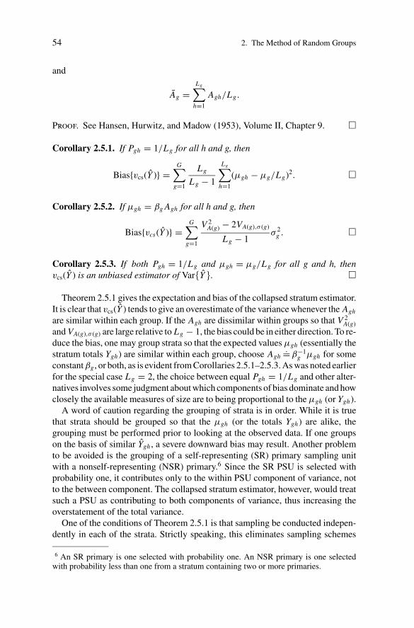
Proof. See Hansen, Hurwitz, and Madow (1953), Volume II, Chapter 9. �

Corollary 2.5.1. If Pgh = 1/Lg for all h and g, then

Bias{vcs(Y )} =G∑

g=1

Lg

Lg − 1

Lg∑h=1

(μgh − μg/Lg)2. �

Corollary 2.5.2. If μgh = βg Agh for all h and g, then

Bias{vcs(Y )} =G∑

g=1

V 2A(g) − 2VA(g),σ (g)

Lg − 1σ 2

g . �

Corollary 2.5.3. If both Pgh = 1/Lg and μgh = μg/Lg for all g and h, thenvcs(Y ) is an unbiased estimator of Var{Y}. �

Theorem 2.5.1 gives the expectation and bias of the collapsed stratum estimator.It is clear that vcs(Y ) tends to give an overestimate of the variance whenever the Agh

are similar within each group. If the Agh are dissimilar within groups so that V 2A(g)

and VA(g),σ (g) are large relative to Lg − 1, the bias could be in either direction. To re-duce the bias, one may group strata so that the expected values μgh (essentially thestratum totals Ygh) are similar within each group, choose Agh = β−1

g μgh for someconstant βg , or both, as is evident from Corollaries 2.5.1–2.5.3. As was noted earlierfor the special case Lg = 2, the choice between equal Pgh = 1/Lg and other alter-natives involves some judgment about which components of bias dominate and howclosely the available measures of size are to being proportional to the μgh (or Ygh).

A word of caution regarding the grouping of strata is in order. While it is truethat strata should be grouped so that the μgh (or the totals Ygh) are alike, thegrouping must be performed prior to looking at the observed data. If one groupson the basis of similar Ygh , a severe downward bias may result. Another problemto be avoided is the grouping of a self-representing (SR) primary sampling unitwith a nonself-representing (NSR) primary.6 Since the SR PSU is selected withprobability one, it contributes only to the within PSU component of variance, notto the between component. The collapsed stratum estimator, however, would treatsuch a PSU as contributing to both components of variance, thus increasing theoverstatement of the total variance.

One of the conditions of Theorem 2.5.1 is that sampling be conducted indepen-dently in each of the strata. Strictly speaking, this eliminates sampling schemes

6 An SR primary is one selected with probability one. An NSR primary is one selectedwith probability less than one from a stratum containing two or more primaries.

P1: OTE/SPH P2: OTE



such as controlled selection, where a dependency exists between the selections indifferent strata. See, e.g., Goodman and Kish (1950) and Ernst (1981). Neverthe-less, because little else is available, the collapsed stratum estimator is often usedto estimate the variance for controlled selection designs. The theoretical proper-ties of this practice are not known, although Brooks (1977) has investigated themempirically. Using 1970 Census data on labor force participation, school enroll-ment, and income, the bias of the collapsed stratum estimator was computed forthe Census Bureau’s Current Population Survey (CPS). The reader will note thatin this survey the PSUs were selected using a controlled selection procedure (seeHanson (1978)). In almost every instance the collapsed stratum estimator resultedin an overstatement of the variance. For estimates concerned with Blacks, the ratiosof the expected value of the variance estimator to the true variance were almostalways between 1.0 and 2.0, while for Whites the ratios were between 3.0 and 4.0.

Finally, Wolter and Causey (1983) have shown that the collapsed stratum estima-tor may be seriously upward biased for characteristics related to labor force statusfor a sampling design where counties are the primary sampling units. The resultssupport the view that the more effective the stratification is in reducing the true vari-ance of estimate, the greater the bias in the collapsed stratum estimator of variance.

In discussing the collapsed stratum estimator, we have presented the relativelysimple situation where one unit is selected from each stratum. We note, however,that mixed strategies for variance estimation are available, and even desirable,depending upon the nature of the sampling design. To illustrate a mixed strategyinvolving the collapsed stratum estimator, suppose that there are L = L ′ + L ′′

strata, where one unit is selected independently from each of the first L ′ strataand two units are selected from each of the remaining L ′′ strata. Suppose thatthe sampling design used in these latter strata is such that it permits an unbiasedestimator of the within stratum variance. Then, for an estimator of the form

Y =L∑

h=1

Yh

=L ′∑

h=1

Yh +L∑

h=L ′+1

Yh

=G ′∑

g=1

L ′g∑

h=1

Ygh +L∑

h=L ′+1

Yh,

L ′ =G ′∑

g=1

L ′g,

we may estimate the variance by

v(Y ) =G ′∑

g=1

L ′g

L ′g − 1

L ′g∑

h=1

(Ygh − PghYg)2 +L∑

h=L ′+1

v(Yh), (2.5.9)

where v(Yh), for h = L ′ + 1, . . . , L , denotes an unbiased estimator of the variance

P1: OTE/SPH P2: OTE



of Yh based upon sampling within the h-th stratum. In this illustration, the collapsedstratum estimator is only used for those strata where one primary unit is sampledand another, presumably unbiased, variance estimator is used for those strata wheremore than one primary unit is sampled. Another illustration of a mixed strategyoccurs in the case of self-representing (SR) primary units. Suppose now that theL ′′ strata each contain one SR primary, and that the L ′ are as before. The varianceestimator is again of the form (2.5.9), where the v(Yh) now represent estimators ofthe variance due to sampling within the self-representing primaries.

As we have seen, the collapsed stratum estimator is usually, though not nec-essarily, upward biased, depending upon the measure of size Agh and its relationto the stratum totals Ygh . In an effort to reduce the size of the bias, several au-thors have suggested alternative variance estimators for one-per-stratum samplingdesigns:

(a) The method of Hartley, Rao, and Kiefer (1969) relies upon a linear modelconnecting the Yh with one or more known measures of size. No collapsingof strata is required. Since the Yh are unknown, the model is fit using the Yh .Estimates σ 2

h of the within stratum variances σ 2h are then prepared from the

regression residuals, and the overall variance is estimated by

v(Y ) =L∑

h=1

σ 2h .

The bias of this statistic as an estimator of Var{Y} is a function of the errorvariance of the true Yh about the assumed regression line.

(b) Fuller’s (1970) method depends on the notion that the stratum boundariesare chosen by a random process prior to sample selection. This preliminarystage of randomization yields nonnegative joint inclusion probabilities forsampling units in the same stratum. Without this randomization, such jointinclusion probabilities are zero. The Yates–Grundy (1953) estimator may thenbe used for estimating Var{Y}, where the inclusion probabilities are specifiedby Fuller’s scheme. The estimator incurs a bias in situations where the stratumboundaries are not randomized in advance.

(c) The original collapsed stratum estimator (2.5.2) was derived via the supposi-tion that the primaries are selected with replacement from within the collapsedstrata. Alternatively, numerous variance estimators may be derived by hypoth-esizing some without replacement sampling scheme within collapsed strata. Asimple possibility is

v(Y ) =G∑

g=1

(1 − 2/Ng)(Yg1 − Yg2)2,

where Ng is the number of primary units in the g-th collapsed stratum. Forthis estimator, srs wor sampling is assumed and (1 − 2/Ng) is the finitepopulation correction. Shapiro and Bateman (1978) have suggested anotherpossibility, where Durbin’s (1967) sampling scheme is hypothesized within

P1: OTE/SPH P2: OTE


2.6. Stability of the Random Group Estimator of Variance 57

collapsed strata. The authors suggest using the Yates and Grundy (1953)variance estimator with the values of the inclusion probabilities specified byDurbin’s scheme. The motivation behind all such alternatives is that varianceestimators derived via without replacement assumptions should be less bi-ased for one-per-stratum designs than estimators derived via with replacementassumptions.

The above methods appear promising for one-per-stratum designs. In fact, eachof the originating authors gives an example where the new method is less biasedthan the collapsed stratum estimator. More comparative studies of the methods areneeded, though, before a definitive recommendation can be made about preferencesfor the various estimators.

2.6. Stability of the Random GroupEstimator of Variance

In most descriptive surveys, emphasis is placed on estimating parameters θ suchas a population mean, a population total, a ratio of two population totals, and soon. An estimator of variance is needed at the analysis stage in order to interpret thesurvey results and to make statistical inferences about θ . The variance of the surveyestimator θ is also of importance at the design stage, where the survey statisticianis attempting to optimize the survey design and to choose a large enough sampleto produce the desired levels of precision for θ . A subordinate problem in mostsurveys, though still a problem of importance, is the stability or precision of thevariance estimator. A related question in the context of the present chapter is “Howmany random groups are needed?”

One general criterion for assessing the stability of the random group estimator

v( ˆθ ) is its coefficient of variation,

CV{v( ˆθ )} = [Var{v( ˆθ )}]1/2/Var{ ˆθ}.

We shall explore the CV criterion in this section. Another general criterion is theproportion of intervals

( ˆθ − c{v( ˆθ )}1/2, ˆθ + c{v( ˆθ )}1/2)

that contain the true population parameter θ , where c is a constant, often basedupon normal or Student’s t theory. This criterion will be addressed in Appendix C.Finally, the quality of a variance estimator may be assessed by its use in otherstatistical analyses, though no results about such criteria are presented in thisbook.

With respect to the CV criterion, we begin with the following theorem.

P1: OTE/SPH P2: OTE



Theorem 2.6.1. Let θ1, . . . , θk be independent and identically distributed randomvariables, and let v( ˆθ ) be defined by (2.2.1). Then

CV{v( ˆθ )} ={

β4(θ1) − (k − 3)/(k − 1)

k

}1/2

, (2.6.1)

where

β4(θ1) = E{(θ1 − μ)4}[E{(θ1 − μ)2}]2

,

μ = E{θ1}.

Proof. Since the θα are independent, we have

E{v2( ˆθ )} = 1

k4

k∑α=1

κ4(θα)

+ 2

k4

(1 + 2

(k − 1)2

) k∑α=1

k∑β>α

κ2(θα)κ2(θβ),

where

κ4(θα) = E{(θα − μ)4},κ2(θα) = E{(θα − μ)2}.

And by the identically distributed condition,

Var{v( ˆθ )} = 1

k3κ4(θ1) + k − 1

k3

k2 − 2k + 3

(k − 1)2κ2

2 (θ1) − E2{v( ˆθ )}.

The result follows by the definition of the coefficient of variation. �

From this theorem, we see that the CV of the variance estimator depends uponboth the kurtosis β4(θ1) of the estimator and the number of groups k. If k is small,the CV will be large and the variance estimator will be of low precision. If thedistribution of θ1 has an excess of values near the mean and in the tails, the kurtosisβ4(θ1) will be large and the variance estimator will be of low precision. When k islarge, we see that the CV2 is approximately inversely proportional to the number ofgroups,

CV2{v( ˆθ )} = β4(θ1) − 1

k.

Theorem 2.6.1 can be sharpened for specific estimators and sampling designs.Two common cases are treated in the following corollaries, which we state withoutproof.

Corollary 2.6.1. A simple random sample with replacement is divided into kgroups of m = n/k units each. Let θα denote the sample mean based on the α-th

P1: OTE/SPH P2: OTE



group, let ˆθ = ∑kα=1 θα/k = ∑n

i=1 yi/n, and let v( ˆθ ) be defined by (2.2.1). Then,

CV{v( ˆθ )} ={

β4(θ1) − (k − 3)/(k − 1)

k

}1/2

, (2.6.2)

where

β4(θ1) = β4/m + 3(m − 1)/m,

β4 =

N∑i=1

(Yi − Y )4/N

{N∑

i=1

(Yi − Y )2/N

}2. �

Corollary 2.6.2. A pps wr sample is divided into k groups of m = n/k unitseach. Let

θα = 1

m

m∑i=1

yi/pi

denote the usual estimator of the population total based on the α-th group, let

ˆθ =k∑

α=1

θα/k = 1

n

n∑i=1

yi/pi ,

and let v( ˆθ ) be defined by (2.2.1). Then,

CV{v( ˆθ )} ={

β4(θ1) − (k − 3)/(k − 1)

k

}1/2

, (2.6.3)

where

β4(θ1) = β4/m + 3(m − 1)/m,

β4 =

N∑i=1

(Zi − Z )4/N

{N∑

i=1

(Zi − Z )2/N

}2,

Zi = Yi/pi . �

Both corollaries work with an estimator ˆθ that is in the form of a sample mean,first for the y-variable and second for the z-variable. Correspondingly, the firstcorollary expresses the CV as a function of the kurtosis of the y-variable, while thesecond corollary expresses the CV as a function of the kurtosis of the z-variable.In this latter case, it is the distribution of z that is important, and when there is anexcess of observations in the tail of this distribution, then β4 is large, making β4(θ1)

large and the precision of v( ˆθ ) low. Both corollaries are important in practical

P1: OTE/SPH P2: OTE



applications because it may be easier to interpret the kurtosis of y or z than thatof θ1.

As has been observed, CV{v( ˆθ )} is an increasing function of β4(θ1) and a de-creasing function of k. The size of the random groups m exerts a minor influence

on β4(θ1) and thus on the CV{v( ˆθ )}. Because the kurtosis β4(θ1) is essentially ofthe form a/m + b, where a and b are constants, it will decrease significantly as mincreases initially from 1. As m becomes larger and larger, however, a law of di-minishing returns takes effect and the decrease in the kurtosis β4(θ1) becomes lessimportant. The marginal decrease in β4(θ1) for larger and larger m is not adequateto compensate for the necessarily decreased k. Thus, the number of groups k has

more of an impact on decreasing the CV{v( ˆθ )} and increasing the precision of thevariance estimate than does the size of the groups m.

While Theorem 2.6.1 and its corollaries were stated for the case of independentrandom groups, we may regard these results as approximate in the more commonsituation of without replacement sampling, particularly in large populations withsmall sampling fractions. This is demonstrated by Hansen, Hurwitz, and Madow’s(1953) result that

CV{v( ˆθ )} = (N − 1)

N (n − 1)

{{(n − 1)2

n− n − 1

n(N − 1)[(n − 2)(n − 3) − (n − 1)]

− 4(n − 1)(n − 2)(n − 3)

n(N − 1)(N − 2)− 6(n − 1)(n − 2)(n − 3)

n(N − 1)(N − 2)(N − 3)

}β4

+{

(n − 1)N

n(N − 1)[(n − 1)2 + 2]

+ 2(n − 1)(n − 2)(n − 3)N

n(N − 1)(N − 2)+ 3(n − 1)(n − 2)(n − 3)N

n(N − 1)(N − 2)(N − 3)

− N 2(n − 1)2

(N − 1)2

}}1/2

(2.6.4)

for srs wor with ˆθ = y and k = n, m = 1. Clearly, when N and n are large and thesampling fraction n/N is small, (2.6.4) and (2.6.2) are approximately equal to oneanother. Based on this result, we suggest that Theorem 2.6.1 and its corollariesmay be used to a satisfactory approximation in studying the stability of the randomgroup variance estimator for modern complex sample surveys, even for withoutreplacement designs and nonindependent random groups.

Theorem 2.6.1 and its corollaries may be used to address two important ques-tions: “How many random groups should be used?” and “What values of m and kare needed to meet a specified level of precision (i.e., a specified level of CV{v( ˆθ )},say CV∗)?”

The question about the number of random groups k involves many considera-tions, including both precision and cost. From a precision perspective, as has beennoted, we would like to choose k as large as possible. From a cost perspective, how-ever, increasing k implies increasing computational costs. Thus, the optimum valueof k will be one that compromises and balances the cost and precision requirements.

P1: OTE/SPH P2: OTE



These requirements will, of course, vary from one survey to another. In one case,the goals of the survey may only seek to obtain a rough idea of the characteristicsof a population, and cost considerations may outweigh precision considerations,suggesting that the optimum value of k is low. On the other hand, if major pol-icy decisions are to be based on the survey results, precision considerations mayprevail, suggesting a large value of k.

To show that a formal analysis of the cost–precision trade-off is possible, con-

sider the simple case of srs wor where the sample mean ˆθ = y is used to estimatethe population mean Y . If the random group estimator of variance is computedaccording to the relation

v( ˆθ ) = 1

k(k − 1)

k∑α=1

(θα − ˆθ )(θα − ˆθ ),

then (m + 3)k + 1 addition or subtraction instructions and 2k + 3 multiplicationor division instructions are used. Now suppose that C dollars are available in thesurvey budget for variance calculations and c1 and c2 are the per unit costs ofan addition or subtraction instruction and a multiplication or division instruction,

respectively. Then, m and k should be chosen to minimize CV{v( ˆθ )} subject to thecost constraint

{(m + 3)k + 1}c1 + (2k + 3)c2 ≤ C. (2.6.5)

As has been observed, however, CV{v( ˆθ )} is, to a good approximation, a decreasingfunction of k, and thus the approximate optimum is the largest value of k (and thecorresponding m) that satisfies the constraint (2.6.5). In multipurpose surveyswhere two or more statistics are to be published, the objective function may bea linear combination of the individual CVs or the CV associated with the mostimportant single statistic. Although the above analysis was for the simple case ofsrs wor and the sample mean, it may be extended in principle to complex surveydesigns and estimators.

To answer the second question, we suggest setting (2.6.1), (2.6.2), or (2.6.3)equal to the desired level of precision CV∗. Then one can study the values of(m, k) needed to meet the precision constraint. Usually, many alternative valuesof (m, k) will be satisfactory, and the one that is preferred will be the one thatminimizes total costs. In terms of the formal analysis, the cost model (2.6.5) is nowthe objective function to be minimized subject to the constraint on the coefficient ofvariation

CV{v( ˆθ )} ≤ CV∗.

In practical applications, some knowledge of the kurtosis β4(θ1) (or β4) will benecessary in addressing either of these two questions. If data from a prior surveyare available, either from the same or similar populations, then such data shouldbe used to estimate β4(θ1). In the absence of such data, some form of subjectivejudgment or expert opinion will have to be relied upon.

P1: OTE/SPH P2: OTE



Table 2.6.1. Bernoulli Distribution

In this connection, Tables 2.6.1 through 2.6.11 present information about 11families of distributions, some discrete, some continuous, and one of a mixedtype. Each table contains six properties of the associated distribution:

(i) the density function,(ii) the constraints on the parameters of the distribution,

(iii) plots of the distribution for alternative values of the parameters,(iv) the mean,(v) the variance, and

(vi) the kurtosis.

These tables may be useful in developing some idea of the magnitude of thekurtosis β4(θ1) (or β4). Simply choose the distribution that best represents thefinite population under study and read the theoretical value of the kurtosis for thatdistribution. The choice of distribution may well be a highly subjective one, inwhich case the kurtosis could only be regarded as an approximation to the truekurtosis for the population under study. Such approximations, however, may wellbe adequate for purposes of planning the survey estimators and variance estimators.If the chosen distribution is intended to represent the distribution of the estimator

P1: OTE/SPH P2: OTE



Table 2.6.2. Discrete Uniform Distribution

θ1, then the tabular kurtosis is β4(θ1), whereas if the distribution represents the unitvalues Yi or Zi , then the tabular kurtosis is β4.

The kurtosis β4(θ1) (or β4) is invariant under linear transformations of θ1 (orYi or Zi ). Therefore, if a given finite population can be represented by a lineartransformation of one of the 11 distributions, then the kurtosis of the originaldistribution applies. If the population cannot be represented by any of the 11distributions or by linear transformations thereof, then see Johnson and Kotz (1969,1970a, 1970b) for discussion of a wide range of distributions.

To illustrate the utility of the tables, suppose a given survey is concerned withthree variables, where the unit values are distributed approximately as a uniform, anormal, and a �(6/7, 1) random variable, respectively. The corresponding valuesof β4 are then 9/5, 3, and 10. Table 2.6.12 gives the corresponding values of

CV{v( ˆθ )} for srs wor of size n = 1000, where sample means are used to estimate

P1: OTE/SPH P2: OTE



Table 2.6.3. Poisson Distribution

population means. If CV{v( ˆθ )} is to be no larger than 15% for each of the threesurvey variables, then at least k = 200 random groups are needed.

2.7. Estimation Based on Order Statistics

In view of the computational simplicity of the random group estimator, one may

question the need for still “quicker” estimators of the variance of ˆθ or θ . There maybe circumstances where the additional simplicity of an estimator based, say, on therange may be useful. Also, estimators based on the range or on quasiranges maybe robust in some sense and may be used to identify errors in the calculation ofthe random group estimator. This section, then, is devoted to a brief discussion ofsuch estimators. For additional information, the reader is referred to David (1970).The estimators described here have received little previous attention in the surveysampling literature.

P1: OTE/SPH P2: OTE


2.7. Estimation Based on Order Statistics 65

Table 2.6.4. Logarithmic Series Distribution

The specific problem that we shall address is that of estimating

σ[defn]= [k · Var{ ˆθ}]1/2.

Given an estimator σ of σ , we may estimate the standard error of ˆθ or θ by σ /k1/2.As before, we let θ1, . . . , θk denote the k random group estimators of θ , and we

let

θ(1), . . . , θ(k)

denote the observations ordered from smallest to largest. We define the range

W = θ(k) − θ(1)

and the i-th quasirange

W(i) = θ(k+1−i) − θ(i),

for 1 ≤ i ≤ [k/2], where the notation [x] signifies the largest integer ≤ x . Notethat the range and the first quasirange are identical.

P1: OTE/SPH P2: OTE



Table 2.6.5. Uniform Distribution

The utility of the range for checking calculations is easily seen. Letting v( ˆθ )

denote the random group estimator, the ratio W 2/v( ˆθ ) is algebraically bounded by

W 2/v( ˆθ ) ≤ 2k(k − 1),

W 2/v( ˆθ ) ≥{

4(k − 1), k even,4k2/(k + 1), k odd.

The upper bound results from a sample configuration with k − 2 observations at ˆθ

and θ(1) and θ(k) at equal distances below and above ˆθ . The lower bound correspondsto half the observations at one extreme θ(k) and half (plus 1 if k is odd) at the other

θ(1). Consequently, if the computed value of v( ˆθ ) is larger than its upper bound

W 2/4(k − 1), k even,W 2/(k + 1)/4k2, k odd,

P1: OTE/SPH P2: OTE



Table 2.6.6. Beta Distribution

or smaller than its lower bound

W 2/2k(k − 1),

then an error has been made either in the computation of the random groupestimator or in the computation of the range.

Ranges and quasiranges form the basis for some extremely simple estimatorsof σ . The first of these is

σ1 = W/dk, (2.7.1)

where dk =E {W/σ } and the expectation operator, E , is with respect to an as-sumed parent distribution for the θα . For the time being, we shall assume that theθα(α = 1, . . . , k) comprise a random sample from the N (θ, σ 2) distribution. For

P1: OTE/SPH P2: OTE



Table 2.6.7. Triangular Distribution

this normal parent, values of dk are given in the second column of Table 2.7.1 fork = 2, 3, . . . , 100. The efficiency of σ1, is very good for k ≤ 12.

In normal samples, however, the efficiency of σ1 declines with increasing k, andat a certain point estimators based on the quasiranges will do better. It has beenshown that σ1 is more efficient than any quasirange for k ≤ 17, but thereafter amultiple of W(2) is more efficient, to be in turn replaced by a multiple of W(3) fork ≥ 32, and so on. Table 2.7.1 also presents the appropriate divisors for W(i) fori = 2, 3, . . . , 9 and k = 2, 3, . . . , 100.

Very efficient estimators can be constructed from thickened ranges, e.g., W +W(2) + W(4), and other linear combinations of quasiranges. A typical estimator is

σ2 = (W + W(2) + W(4))/ek, (2.7.2)

where ek = E {(W + W(2) + W(4))/σ } may be obtained by summing the appro-priate elements of Table 2.7.1. For k = 16, the estimator σ2 has efficiency97.5%.

P1: OTE/SPH P2: OTE



Table 2.6.8. Standard Normal Distribution

Table 2.7.2 presents several unbiased estimators of σ and their associated effi-ciencies for k = 2, 3, . . . , 100. Column 2 gives the most efficient estimator, say σ3,based on a single quasirange (i ≤ 9); Column 3 gives its corresponding efficiency;Column 4 gives the most efficient estimator, say σ4, based on a linear combinationof two quasiranges (i and i ′ ≤ 9); and Column 5 gives its corresponding efficiency.The efficiencies,

eff{σ3} = Var{σ }/Var{σ3},eff{σ4} = Var{σ }/Var{σ4},

are with respect to the minimum variance unbiased estimator

σ = �[(k − 1)/2]

[2/(k − 1)]1/2�(k/2)

[k∑α

(θα − ˆθ )2/(k − 1)

]1/2

.

A final important estimator of σ is

σ5 = 2√

π

k(k − 1)

k∑α=1

[α − (k + 1)/2]θ(α). (2.7.3)

P1: OTE/SPH P2: OTE



Table 2.6.9. Gamma Distribution

Barnett et al. (1967) have found that σ5 is highly efficient (>97.8%) and morerobust against outliers than σ1 and σ .

Example 2.2.1. k = 16 random groups are to be used. Then, the estimators of σ

take the form

σ1 = W/3.531,

σ2 = (W + W(2) + W(4))/(3.531 + 2.569 + 1.526)

= (W + W(2) + W(4))/7.626,

σ3 = W/3.531

= 0.283W,

σ4 = 0.168(W + 1.216W(3)),

σ5 = 2√

π

16(15)

16∑α=1

(α − 17/2)θ(α).

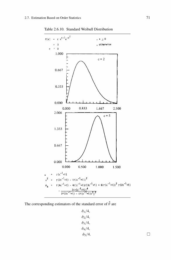
P1: OTE/SPH P2: OTE



Table 2.6.10. Standard Weibull Distribution

The corresponding estimators of the standard error of ˆθ are

σ1/4,

σ2/4,

σ3/4,

σ4/4,

σ5/4. �

P1: OTE/SPH P2: OTE



Table 2.6.11. Mixed Uniform Distribution

The methods discussed here could be criticized on the grounds that the estimatorsare bound to be both inefficient and overly sensitive to the shape of the parentdistribution of the θα . There is evidence, however, that both criticisms may bemisleading (see David (1970)). As we have already seen, the loss in efficiencyis usually unimportant. Furthermore, the ratio E {W/σ } is remarkably stable formost reasonable departures from normality. Table 2.7.3 illustrates the stabilitywell. The entries in the table are the percent bias in the efficient estimators σ3

and σ4 (constructed using normality assumptions) when the parent distributionis actually uniform or exponential. For the uniform distribution, the percent biasis quite trivial for most values of k between 2 and 100. The bias is somewhatmore important for the skewed parent (i.e., the exponential distribution), but notalarmingly so. In almost all cases, the estimators tend towards an underestimate.

P1: OTE/SPH P2: OTE


2.8. Deviations from Strict Principles 73

Table 2.6.12. CV{v( ˆθ )} for n = 1000

β4

m k 9/5 3 10

500 2 1.41379 1.41421 1.41669

250 4 0.81576 0.81650 0.82077

200 5 0.70626 0.70711 0.71204

125 8 0.53340 0.53452 0.54103

100 10 0.47013 0.47140 0.47877

50 20 0.32259 0.32444 0.33506

40 25 0.28659 0.28868 0.30056

20 50 0.19904 0.20203 0.21867

10 100 0.13785 0.14213 0.16493

8 125 0.12218 0.12700 0.15208

5 200 0.09408 0.10025 0.13058

4 250 0.08266 0.08962 0.12261

2 500 0.05299 0.06331 0.10492

1 1000 0.02832 0.04474 0.09488

Cox (1954) suggests that the ratio E {W/σ } does not depend on the skewness ofthe parent distribution but only on the kurtosis. With approximate knowledge ofthe kurtosis (e.g., from a prior survey of a similar population) one may use Cox’stables to correct for the bias.

The stability of E {W/σ } is, of course, of central importance in applying thesemethods to samples from finite populations because the random group estimatorsθα cannot, strictly speaking, be viewed as normally distributed. The fact that theratio E {W/σ } is quite stable lends support to the use of these estimators in finite-population sampling. Further support is derived from the various central limittheorems given in Appendix B. In many cases, when the size m of the randomgroups is large and the number of groups k is fixed, the θα will behave, roughlyspeaking, as a random sample from a normal distribution and the methods presentedin this section will be appropriate.

2.8. Deviations from Strict Principles

The fundamental principles of the random group method were presented in Sec-tions 2.2 and 2.4 for the independent and nonindependent cases, respectively. Inpractice, however, there are often computational or other advantages to some devi-ation from these principles. We may suggest a modified random group procedureif it both results in a substantial cost savings and gives essentially the same re-sults as the unmodified procedure. In this section, we discuss briefly two suchmodifications.

P1: OTE/SPH P2: OTE



Table 2.7.1. Denominator dk of Unbiased Estimator of σ Based on the i-thQuasirange for Samples of k from N (θ, σ 2)

k i = 1 i = 2 i = 3 i = 4 i = 5 i = 6 i = 7 i = 8 i = 9

2 1.128

3 1.692

4 2.058 0.594

5 2.325 0.990

6 2.534 1.283 0.403

7 2.704 1.514 0.705

8 2.847 1.704 0.945 0.305

9 2.970 1.864 1.143 0.549

10 3.077 2.002 1.312 0.751 0.245

11 3.172 2.123 1.457 0.923 0.449

12 3.258 2.231 1.585 1.073 0.624 0.205

13 3.335 2.328 1.699 1.205 0.776 0.381

14 3.406 2.415 1.802 1.323 0.911 0.534 0.176

15 3.471 2.495 1.895 1.429 1.031 0.670 0.330

16 3.531 2.569 1.980 1.526 1.140 0.792 0.467 0.154

17 3.587 2.637 2.058 1.614 1.238 0.902 0.590 0.291

18 3.640 2.700 2.131 1.696 1.329 1.003 0.701 0.415 0.137

19 3.688 2.759 2.198 1.771 1.413 1.095 0.803 0.527 0.261

20 3.734 2.815 2.261 1.841 1.490 1.180 0.896 0.629 0.373

21 3.778 2.867 2.320 1.907 1.562 1.259 0.982 0.724 0.476

22 3.819 2.916 2.376 1.969 1.630 1.333 1.063 0.811 0.571

23 3.858 2.962 2.428 2.027 1.693 1.402 1.137 0.892 0.659

24 3.895 3.006 2.478 2.081 1.753 1.467 1.207 0.967 0.740

25 3.930 3.048 2.525 2.133 1.810 1.528 1.273 1.038 0.817

26 3.964 3.088 2.570 2.182 1.863 1.585 1.335 1.105 0.888

27 3.996 3.126 2.612 2.229 1.914 1.640 1.394 1.168 0.956

28 4.027 3.162 2.653 2.273 1.962 1.692 1.450 1.227 1.019

29 4.057 3.197 2.692 2.316 2.008 1.741 1.503 1.284 1.079

30 4.085 3.231 2.729 2.357 2.052 1.788 1.553 1.337 1.136

31 4.112 3.263 2.765 2.396 2.094 1.833 1.601 1.388 1.190

32 4.139 3.294 2.799 2.433 2.134 1.876 1.647 1.437 1.242

33 4.164 3.324 2.832 2.469 2.173 1.918 1.691 1.484 1.291

34 4.189 3.352 2.864 2.503 2.210 1.957 1.733 1.528 1.339

35 4.213 3.380 2.895 2.537 2.245 1.995 1.773 1.571 1.384

36 4.236 3.407 2.924 2.569 2.280 2.032 1.812 1.612 1.427

37 4.258 3.433 2.953 2.600 2.313 2.067 1.849 1.652 1.469

38 4.280 3.458 2.981 2.630 2.345 2.101 1.886 1.690 1.509

39 4.301 3.482 3.008 2.659 2.376 2.134 1.920 1.726 1.547

40 4.321 3.506 3.034 2.687 2.406 2.166 1.954 1.762 1.585

41 4.341 3.529 3.059 2.714 2.435 2.197 1.986 1.796 1.621

42 4.360 3.551 3.083 2.740 2.463 2.227 2.018 1.829 1.655

43 4.379 3.573 3.107 2.766 2.491 2.256 2.048 1.861 1.689

44 4.397 3.594 3.130 2.791 2.517 2.284 2.078 1.892 1.721

45 4.415 3.614 3.153 2.815 2.543 2.311 2.107 1.922 1.753

P1: OTE/SPH P2: OTE



Table 2.7.1. (Cont.)

k i = 1 i = 2 i = 3 i = 4 i = 5 i = 6 i = 7 i = 8 i = 9

46 4.432 3.634 3.175 2.839 2.568 2.337 2.135 1.951 1.784

47 4.449 3.654 3.196 2.862 2.592 2.363 2.162 1.980 1.813

48 4.466 3.673 3.217 2.884 2.616 2.388 2.188 2.007 1.842

49 4.482 3.691 3.237 2.906 2.639 2.413 2.214 2.034 1.870

50 4.498 3.709 3.257 2.927 2.662 2.436 2.238 2.060 1.897

51 4.513 3.727 3.276 2.948 2.684 2.460 2.263 2.086 1.924

52 4.528 3.744 3.295 2.968 2.705 2.482 2.286 2.110 1.950

53 4.543 3.761 3.313 2.988 2.726 2.504 2.310 2.135 1.975

54 4.557 3.778 3.331 3.007 2.746 2.526 2.325 2.158 1.999

55 4.571 3.794 3.349 3.026 2.766 2.547 2.354 2.181 2.023

56 4.585 3.810 3.366 3.044 2.786 2.567 2.376 2.204 2.047

57 4.599 3.825 3.383 3.062 2.805 2.587 2.397 2.226 2.069

58 4.612 3.840 3.400 3.080 2.824 2.607 2.417 2.247 2.092

59 4.625 3.855 3.416 3.097 2.842 2.626 2.437 2.268 2.113

60 4.638 3.870 3.432 3.114 2.860 2.645 2.457 2.288 2.135

61 4.651 3.884 3.447 3.131 2.878 2.663 2.476 2.308 2.156

62 4.663 3.898 3.463 3.147 2.895 2.681 2.495 2.328 2.176

63 4.675 3.912 3.478 3.163 2.912 2.699 2.513 2.347 2.196

64 4.687 3.926 3.492 3.179 2.928 2.716 2.532 2.366 2.215

65 4.699 3.939 3.507 3.194 2.944 2.733 2.549 2.385 2.235

66 4.710 3.952 3.521 3.209 2.960 2.750 2.567 2.403 2.253

67 4.721 3.965 3.535 3.224 2.976 2.767 2.584 2.420 2.272

68 4.733 3.977 3.549 3.239 2.991 2.783 2.601 2.438 2.290

69 4.743 3.990 3.562 3.253 3.006 2.798 2.617 2.455 2.308

70 4.754 4.002 3.575 3.267 3.021 2.814 2.633 2.472 2.325

71 4.765 4.014 3.588 3.281 3.036 2.829 2.649 2.488 2.342

72 4.775 4.026 3.601 3.294 3.050 2.844 2.665 2.504 2.359

73 4.785 4.037 3.613 3.308 3.064 2.859 2.680 2.520 2.375

74 4.796 4.049 3.626 3.321 3.078 2.873 2.695 2.536 2.391

75 4.805 4.060 3.638 3.334 3.091 2.887 2.710 2.551 2.407

76 4.815 4.071 3.650 3.346 3.105 2.901 2.724 2.566 2.423

77 4.825 4.082 3.662 3.359 3.118 2.915 2.739 2.581 2.438

78 4.834 4.093 3.673 3.371 3.131 2.929 2.753 2.596 2.453

79 4.844 4.103 3.685 3.383 3.144 2.942 2.767 2.610 2.468

80 4.853 4.114 3.696 3.395 3.156 2.955 2.780 2.624 2.483

81 4.862 4.124 3.707 3.407 3.169 2.968 2.794 2.638 2.497

82 4.871 4.134 3.718 3.419 3.181 2.981 2.807 2.652 2.511

83 4.880 4.144 3.729 3.430 3.193 2.993 2.820 2.665 2.525

84 4.889 4.154 3.740 3.442 3.205 3.006 2.833 2.679 2.539

85 4.897 4.164 3.750 3.453 3.216 3.018 2.845 2.692 2.553

86 4.906 4.173 3.760 3.464 3.228 3.030 2.858 2.705 2.566

87 4.914 4.183 3.771 3.474 3.239 3.042 2.870 2.717 2.579

88 4.923 4.192 3.781 3.485 3.250 3.053 2.882 2.730 2.592

89 4.931 4.201 3.791 3.496 3.261 3.065 2.894 2.742 2.605

90 4.939 4.211 3.801 3.506 3.272 3.076 2.906 2.754 2.617

P1: OTE/SPH P2: OTE




k i = 1 i = 2 i = 3 i = 4 i = 5 i = 6 i = 7 i = 8 i = 9

91 4.947 4.220 3.810 3.516 3.283 3.087 2.918 2.766 2.630

92 4.955 4.228 3.820 3.526 3.294 3.098 2.929 2.778 2.642

93 4.963 4.237 3.829 3.536 3.304 3.109 2.940 2.790 2.654

94 4.970 4.246 3.839 3.546 3.314 3.120 2.951 2.802 2.666

95 4.978 4.254 3.848 3.556 3.325 3.131 2.963 2.813 2.678

96 4.985 4.263 3.857 3.566 3.335 3.141 2.973 2.824 2.689

97 4.993 4.271 3.866 3.575 3.345 3.152 2.984 2.835 2.701

98 5.000 4.280 3.875 3.585 3.355 3.162 2.995 2.846 2.712

99 5.007 4.288 3.884 3.594 3.364 3.172 3.005 2.857 2.723

100 5.015 4.296 3.892 3.603 3.374 3.182 3.016 2.868 2.734

Source: Table 1 of Harter (1959). Harter’s tables are given to six decimal places. We have truncated(not rounded) his figures to three decimal places.

Table 2.7.2. Most Efficient Unbiased Estimators of σ Based on Quasiranges forSamples of k from N (θ, σ 2)

Based on a Linear Combination of

Two Quasiranges Among Those with

Based on One Quasirange i < i ′ ≤ 9

k Estimate Eff(%) Estimate Eff(%)

2 0.886W1 100.00

3 0.590W1 99.19

4 0.485W1 97.52 0.453(W1 + 0.242W2) 98.92

5 0.429W1 95.48 0.372(W1 + 0.363W2) 98.84

6 0.394W1 93.30 0.318(W1 + 0.475W2) 98.66

7 0.369W1 91.12 0.279(W1 + 0.579W2) 98.32

8 0.351W1 89.00 0.250(W1 + 0.675W2) 97.84

9 0.336W1 86.95 0.227(W1 + 0.765W2) 97.23

10 0.324W1 84.99 0.209(W1 + 0.848W2) 96.54

11 0.315W1 83.13 0.194(W1 + 0.927W2) 95.78

12 0.306W1 81.36 0.211(W1 + 0.923W3) 95.17

13 0.299W1 79.68 0.198(W1 + 1.001W3) 95.00

14 0.293W1 78.09 0.187(W1 + 1.076W3) 94.77

15 0.288W1 76.57 0.177(W1 + 1.147W3) 94.50

16 0.283W1 75.13 0.168(W1 + 1.216W3) 94.18

17 0.278W1 73.76 0.160(W1 + 1.281W3) 93.82

18 0.370W2 72.98 0.153(W1 + 1.344W3) 93.43

19 0.362W2 72.98 0.147(W1 + 1.405W3) 93.02

20 0.355W2 72.91 0.141(W1 + 1.464W3) 92.59

21 0.348W2 72.77 0.136(W1 + 1.520W3) 92.14

22 0.342W2 72.59 0.146(W1 + 1.529W4) 91.78

P1: OTE/SPH P2: OTE








23 0.337W2 72.37 0.141(W1 + 1.588W4) 91.61

24 0.332W2 72.11 0.136(W1 + 1.644W4) 91.42

25 0.328W2 71.82 0.132(W1 + 1.699W4) 91.21

26 0.323W2 71.52 0.128(W1 + 1.752W4) 90.98

27 0.319W2 71.20 0.124(W1 + 1.805W4) 90.73

28 0.316W2 70.86 0.121(W1 + 1.855W4) 90.48

29 0.312W2 70.51 0.118(W1 + 1.905W4) 90.21

30 0.309W2 70.15 0.115(W1 + 1.953W4) 89.93

31 0.306W2 69.78 0.112(W1 + 2.000W4) 89.63

32 0.357W3 69.57 0.109(W1 + 2.046W4) 89.35

33 0.353W3 69.58 0.115(W1 + 2.067W5) 89.11

34 0.349W3 69.57 0.112(W1 + 2.115W5) 88.97

35 0.345W3 69.53 0.110(W1 + 2.161W5) 88.82

36 0.341W3 69.48 0.107(W1 + 2.207W5) 88.66

37 0.338W3 69.41 0.105(W1 + 2.252W5) 88.48

38 0.335W3 69.32 0.103(W1 + 2.296W5) 88.31

39 0.332W3 69.21 0.101(W1 + 2.339W5) 88.12

40 0.329W3 69.10 0.099(W1 + 2.381W5) 87.92

41 0.326W3 68.97 0.097(W1 + 2.423W5) 87.73

42 0.324W3 68.83 0.095(W1 + 2.464W5) 87.52

43 0.321W3 68.68 0.094(W1 + 2.504W5) 87.32

44 0.319W3 68.53 0.092(W1 + 2.543W5) 87.10

45 0.317W3 68.37 0.096(W1 + 2.574W6) 86.97

46 0.352W4 68.22 0.094(W1 + 2.615W6) 86.85

47 0.349W4 68.24 0.093(W1 + 2.655W6) 86.73

48 0.346W4 68.23 0.091(W1 + 2.695W6) 86.60

49 0.344W4 68.22 0.090(W1 + 2.734W6) 86.47

50 0.341W4 68.20 0.088(W1 + 2.772W6) 86.33

51 0.339W4 68.17 0.087(W1 + 2.810W6) 86.19

52 0.336W4 68.12 0.086(W1 + 2.847W6) 86.04

53 0.334W4 68.07 0.084(W1 + 2.884W6) 85.89

54 0.332W4 68.02 0.083(W1 + 2.921W6) 85.73

55 0.330W4 67.95 0.082(W1 + 2.956W6) 85.57

56 0.328W4 67.87 0.137(W2 + 1.682W9) 85.44

57 0.326W4 67.80 0.135(W2 + 1.706W9) 85.46

58 0.324W4 67.71 0.134(W2 + 1.730W9) 85.47

59 0.322W4 67.62 0.132(W2 + 1.753W9) 85.48

60 0.321W4 67.53 0.130(W2 + 1.777W9) 85.48

61 0.347W5 67.52 0.128(W2 + 1.800W9) 85.47

62 0.345W5 67.52 0.127(W2 + 1.823W9) 85.46

63 0.343W5 67.52 0.125(W2 + 1.846W9) 85.44

P1: OTE/SPH P2: OTE








64 0.341W5 67.50 0.123(W2 + 1.868W9) 85.42

65 0.339W5 67.49 0.122(W2 + 1.890W9) 85.40

66 0.337W5 67.46 0.121(W2 + 1.912W9) 85.36

67 0.335W5 67.44 0.119(W2 + 1.934W9) 85.33

68 0.334W5 67.40 0.118(W2 + 1.955W9) 85.29

69 0.332W5 67.36 0.116(W2 + 1.976W9) 85.24

70 0.330W5 67.32 0.115(W2 + 1.997W9) 85.20

71 0.329W5 67.27 0.114(W2 + 2.018W9) 85.14

72 0.327W5 67.22 0.113(W2 + 2.038W9) 85.09

73 0.326W5 67.16 0.111(W2 + 2.059W9) 85.04

74 0.324W5 67.11 0.110(W2 + 2.079W9) 84.98

75 0.346W6 67.07 0.109(W2 + 2.099W9) 84.91

76 0.344W6 67.03 0.108(W2 + 2.118W9) 84.85

77 0.342W6 67.07 0.107(W2 + 2.138W9) 84.78

78 0.341W6 67.07 0.106(W2 + 2.157W9) 84.71

79 0.339W6 67.06 0.105(W2 + 2.176W9) 84.63

80 0.338W6 67.04 0.104(W2 + 2.195W9) 84.56

81 0.336W6 67.03 0.103(W2 + 2.214W9) 84.48

82 0.335W6 67.01 0.102(W2 + 2.232W9) 84.40

83 0.334W6 66.98 0.101(W2 + 2.251W9) 84.32

84 0.332W6 66.95 0.100(W2 + 2.269W9) 84.23

85 0.331W6 66.92 0.099(W2 + 2.287W9) 84.15

86 0.329W6 66.89 0.099(W2 + 2.305W9) 84.07

87 0.328W6 66.85 0.098(W2 + 2.323W9) 83.97

88 0.327W6 66.81 0.097(W2 + 2.340W9) 83.88

89 0.345W7 66.77 0.096(W2 + 2.358W9) 83.79

90 0.344W7 66.77 0.095(W2 + 2.375W9) 83.70

91 0.342W7 66.77 0.095(W2 + 2.393W9) 83.61

92 0.341W7 66.77 0.094(W2 + 2.409W9) 83.51

93 0.340W7 66.76 0.093(W2 + 2.426W9) 83.42

94 0.338W7 66.75 0.092(W2 + 2.443W9) 83.32

95 0.337W7 66.74 0.092(W2 + 2.459W9) 83.22

96 0.336W7 66.73 0.091(W2 + 2.476W9) 83.12

97 0.335W7 66.71 0.090(W2 + 2.492W9) 83.02

98 0.333W7 66.69 0.090(W2 + 2.508W9) 82.92

99 0.332W7 66.67 0.089(W2 + 2.524W9) 82.82

100 0.331W7 66.65 0.088(W2 + 2.540W9) 82.71

Source: Table 4 of Harter (1959). Harter’s results have been truncated (not rounded) to three decimalplaces.

P1: OTE/SPH P2: OTE



Table 2.7.3. Percent Bias of Estimators of σ that Assume Normality

When Population Is Uniform When Population Is Exponential

Two Two

One Quasiranges One Quasiranges

k Quasirange with i < i ′ ≤ 9 Quasirange with i < i ′ ≤ 9

2 2.33 −11.38

3 2.33 −11.38

4 0.96 1.98 −10.95 −11.27

5 −0.71 1.61 −10.43 −11.16

6 −2.37 1.13 −9.91 −11.01

7 −3.93 0.54 −9.41 −10.84

8 −5.37 −0.11 −8.93 −10.66

9 −6.69 −0.80 −8.49 −10.46

10 −7.90 −1.51 −8.08 −10.26

11 −9.02 −2.22 −7.69 −10.06

12 −10.04 −1.47 −7.32 −10.07

13 −10.99 −1.72 −6.98 −10.00

14 −11.87 −2.01 −6.65 −9.92

15 −12.69 −2.33 −6.34 −9.84

16 −13.46 −2.66 −6.05 −9.75

17 −14.18 −3.01 −5.77 −9.65

18 1.26 −3.37 −11.85 −9.56

19 0.41 −3.74 −11.61 −9.46

20 −0.39 −4.11 −11.37 −9.36

21 −1.15 −4.48 −11.14 −9.25

22 −1.87 −3.11 −10.92 −9.43

23 −2.56 −3.32 −10.71 −9.38

24 −3.22 −3.53 −10.51 −9.33

25 −3.85 −3.75 −10.31 −9.28

26 −4.45 −3.98 −10.12 −9.22

27 −5.03 −4.21 −9.93 −9.16

28 −5.58 −4.45 −9.75 −9.10

29 −6.11 −4.69 −9.58 −9.04

30 −6.63 −4.94 −9.41 −8.98

31 −7.12 −5.18 −9.24 −8.91

32 1.23 −5.43 −12.07 −8.85

33 0.71 −3.95 −11.92 −9.09

34 0.20 −4.11 −11.78 −9.05

35 −0.29 −4.28 −11.63 −9.02

36 −0.77 −4.45 −11.49 −8.98

37 −1.23 −4.63 −11.35 −8.93

38 −1.68 −4.81 −11.22 −8.89

39 −2.11 −4.99 −11.09 −8.85

40 −2.53 −5.17 −10.96 −8.81

41 −2.94 −5.36 −10.83 −8.76

42 −3.34 −5.54 −10.71 −8.72

P1: OTE/SPH P2: OTE





Two Two



43 −3.73 −5.72 −10.59 −8.67

44 −4.10 −5.91 −10.47 −8.62

45 −4.47 −4.45 −10.35 −8.89

46 1.24 −4.59 −12.18 −8.86

47 0.86 −4.73 −12.07 −8.83

48 0.49 −4.88 −11.96 −8.80

49 0.12 −5.02 −11.86 −8.76

50 −0.23 −5.17 −11.75 −8.73

51 −0.58 −5.32 −11.65 −8.70

52 −0.92 −5.46 −11.55 −8.66

53 −1.25 −5.61 −11.45 −8.63

54 −1.57 −5.76 −11.36 −8.59

55 −1.89 −5.91 −11.26 −8.55

56 −2.20 −0.63 −11.17 −10.80

57 −2.50 −0.76 −11.08 −10.78

58 −2.79 −0.89 −10.98 −10.75

59 −3.08 −1.02 −10.89 −10.71

60 −3.37 −1.15 −10.81 −10.67

61 0.95 −1.28 −12.16 −10.64

62 0.66 −1.41 −12.07 −10.60

63 0.37 −1.55 −11.99 −10.56

64 0.09 −1.67 −11.91 −10.53

65 −0.19 −1.81 −11.83 −10.49

66 −0.46 −1.94 −11.75 −10.46

67 −0.73 −2.07 −11.67 −10.42

68 −0.99 −2.20 −11.59 −10.38

69 −1.25 −2.34 −11.51 −10.35

70 −1.50 −2.47 −11.44 −10.31

71 −1.75 −2.59 −11.36 −10.27

72 −1.99 −2.73 −11.29 −10.24

73 −2.23 −2.85 −11.22 −10.20

74 −2.47 −2.98 −11.14 −10.17

75 1.01 −3.11 −12.21 −10.13

76 0.77 −3.24 −12.14 −10.09

77 0.53 −3.36 −12.07 −10.05

78 0.30 −3.49 −12.01 −10.02

79 0.07 −3.62 −11.94 −9.98

80 −0.16 −3.74 −11.87 −9.95

81 −0.38 −3.87 −11.81 −9.91

82 −0.60 −3.99 −11.74 −9.88

83 −0.82 −4.11 −11.68 −9.84

P1: OTE/SPH P2: OTE





Two Two



84 −1.04 −4.24 −11.62 −9.81

85 −1.25 −4.36 −11.55 −9.77

86 −1.45 −4.48 −11.49 −9.74

87 −1.66 −4.60 −11.43 −9.70

88 −1.86 −4.72 −11.37 −9.67

89 1.06 −4.83 −12.25 −9.63

90 0.85 −4.95 −12.19 −9.60

91 0.65 −5.07 −12.13 −9.56

92 0.45 −5.19 −12.08 −9.53

93 0.25 −5.30 −12.02 −9.49

94 0.05 −5.42 −11.96 −9.46

95 −0.14 −5.53 −11.91 −9.43

96 −0.33 −5.64 −11.85 −9.39

97 −0.52 −5.76 −11.80 −9.36

98 −0.70 −5.87 −11.74 −9.32

99 −0.88 −5.98 −11.69 −9.29

100 −1.07 −6.09 −11.63 −9.26

Source: Table 6 of Harter (1959).

The first concerns the “weights” used in preparing the survey estimates. To beprecise, we consider a survey estimator

θ =∑i∈s

Wi Yi (2.8.1)

with weights {Wi }. In a typical survey, the Wi may be a product of several compo-nents, including the reciprocal of the inclusion probability (or the basic weight);an adjustment for nonresponse, undercoverage, and post-stratification; and pos-sibly a seasonal adjustment. Strict adherence to random group principles woulddictate that the adjustments of the basic weights be computed separately withineach random group. That is, the sample is divided into, say, k groups and fromeach group s(α) an estimator

θα =∑

i∈s(α)

Wαi Yi (2.8.2)

is developed of the same functional form as the parent estimator θ . The sum in(2.8.2) is only over units in the α-th random group, and the replicate weights{Wαi} are developed from the inclusion probabilities with adjustments derivedfrom information in the α-th group only. The reader will immediately recognize

P1: OTE/SPH P2: OTE



the computational cost and complexities associated with this procedure. In effectthe weight adjustments must be computed k + 1 times: once for the full-sampleestimator and once for each of the k random group estimators. For extremelylarge samples, the cost associated with these multiple weight adjustments maybe significant. A simpler procedure that sometimes gives satisfactory results is tocompute random group estimates, say θα , using the weight adjustments appropriateto the full sample rather than to the relevant random group. That is, θα is definedas in (2.8.2) and the Wαi are now developed from the inclusion probabilities forthe α-th random group with adjustments derived from all of the information in thefull parent sample. In this way computational advantages are gained because onlyone set of weight adjustments is necessary.

Intuitively, we expect that this shortcut procedure may tend to under-representthe component of variability associated with random error in the weight adjust-ments and thus underestimate the total variance of θ . In some cases, however,Taylor series approximations (see Chapter 6) suggest that this problem is not aserious one. To illustrate, consider a simple situation where the sample is classi-fied into L1i poststrata. The poststratified estimator is in the form of (2.8.1) withWi = W1i (Nh/Nh), where W1i = π−1

i , π is the inclusion probability associatedwith the i-th unit, h is the stratum to which the i-th unit was classified, Nh is theknown number of units in the h-th stratum, Nh = ∑

j∈shW1 j is the full-sample

estimator of Nh , and sh denotes the set of selected units that were classified intothe h-th stratum. The α-th random group estimator is in the form of (2.8.2) with

Wαi = kW1i (Nh/Nh(α)),

Nh(α) =∑

j∈sh (α)

kW1 j ,

and sh(α) denotes the set of units in the α-th random group that were classifiedinto the h-th stratum. Note that the base weight associated with the full sample isWi , and that with the α-th random group is kW1i . Then, from first principles, arandom group estimator of variance is

v2(θ ) = 1

k(k − 1)

k∑α

(θα − θ )2.

Viewing this estimator as a function of (N1(1), . . . , NL(1), . . . , NL(k)) and expandingin a Taylor series about the point (N1, . . . , NL , . . . , NL ) gives

v2(θ ) = 1

k(k − 1)

k∑α

(θα − θ )2,

where

θα =∑s(α)

{kW −11i (Nh/Nh)}Yi

is the α-th random group estimator derived using the full-sample weight adjust-ment Nh/Nh . This shows that the strict random group procedure θα and the

P1: OTE/SPH P2: OTE



modified shortcut procedure θα should give similar results, at least to a localapproximation.

Simmons and Baird (1968) and Bean (1975) have empirically compared theshortcut procedure to the standard procedure using the National Center for HealthStatistics Health Examination Survey. They found that the shortcut procedure gaveslightly worse variance estimates but saved greatly on computational costs.

Wolter, Pedlow, and Wang (2005) compared the shortcut and standard proce-dures using data from the National Longitudinal Survey of Youth, 1997. Theyfound that both procedures produced very similar numerical results. On the basisof these studies, we recommend the shortcut procedure for use in many large-scalemodern surveys.

These comments also apply to the donor pool used in making imputations formissing data. Strict RG principles suggest that the α-th random group should serveas the donor pool for imputing for missing data within the α-th random group forα = 1, . . . , k. An alternative procedure that may give satisfactory results is to letthe entire parent sample serve as the donor pool for imputing for missing datawithin any of the random groups.

The second modification to the random group method concerns the manner inwhich the random groups are formed in the nonindependent case. To illustratethe modification, we suppose the population is divided into L ≥ 1 strata and twoor more PSUs are selected within each stratum using some without replacementsampling scheme. Strict adherence to random group principles would dictate thatrandom groups be formed by randomly selecting one or more of the ultimateclusters from each stratum. In this manner, each random group would have thesame design features as the parent sample. However, if there are only a smallnumber of selected primaries in some or all of the strata, the number of randomgroups, k, will be small and the resulting variance of the variance estimator large.For this situation we may seek a modified random group procedure that is biasedbut leads to greater stability through use of a larger number of random groups. Thefollowing modification may be acceptable:

(i) The ultimate clusters are ordered on the basis of the stratum from which theywere selected. Within a stratum, the ultimate clusters are taken in a natural orrandom order.

(ii) The ultimate clusters are then systematically assigned to k (acceptably large)random groups. For example, the first ultimate cluster may be assigned randomgroup α∗ (a random integer between 1 and k), the second to group α∗ + 1, andso forth in a modulo k fashion.

The heuristic motivation for the modification is quite simple: the bias of the varianceestimator should not be large since the systematic assignment procedure reflectsapproximately the stratification in the sample, while use of increased k shouldreduce the variance of the variance estimator. While there is no general theory tosubstantiate this claim, a small empirical study by Isaki and Pinciaro (1977) is sup-portive. An example involving an establishment survey is reported in Section 2.10.

P1: OTE/SPH P2: OTE



2.9. On the Condition ˆθ = θ for Linear Estimators

At various points in this chapter, we have stated that the mean of the random

group estimators is equal to the parent sample estimator, i.e., ˆθ = θ , whenever theestimator is linear. We shall make similar statements in Chapters 3 and 4 as wetalk about balanced half-samples and the jackknife. We shall now demonstrate themeaning of this statement in the context of Definition 1.5.1 in Section 1.5. This

work clarifies the distinction between v( ˆθ ), v1(θ ), and v2(θ ) and suggests whenthe parent sample estimator θ may be reproduced as the mean of the θα . This latterpoint is of interest from a computational point of view because it is important toknow when θ may be computed as a by-product of the θα calculations and whena separate calculation of θ is required.

Using the notation of Section 1.5, we note that it is sufficient to work with (1.5.3)because the estimator in Definition 1.5.1 satisfies

ˆθ = 1

k

k∑α

θα

= γ0 + γ1ˆθ (1) + · · · + γp

ˆθ (p)

= γ0 + γ1θ (1) + · · · + γp θ (p)

= θ

if and only if

ˆθ ( j) = θ ( j), for j = 1, . . . p,

where

θα = γ0 + γ1θα(1) + · · · + θα(p)

and θα( j) denotes the estimator for the j-th characteristic based on the α-th randomgroup. As a consequence, we condense the notation, letting θ denote an estimatorof the form (1.5.3).

It is easy to establish that not all linear estimators in this form satisfy the propertyˆθ = θ . A simple example is the classical ratio estimator for srs wor. For this case

θ = (y/x)X ,

θα = (yα/xα)X ,

and

ˆθ =(

k−1k∑α

yα/xα

)X .

�= θ .

Unfortunately, it is difficult to specify precisely the class of linear estimators for

P1: OTE/SPH P2: OTE


2.9. On the Condition ˆθ = θ for Linear Estimators 85

which the property does hold. The best we can do is illustrate some cases where itdoes and does not hold.

(i) Suppose that a single-stage sample of fixed size n = mk is selected withoutreplacement and then divided into k random groups according to the prin-ciples given in Section 2.3. The Horvitz–Thompson (H–T) estimator of the

population total satisfies ˆθ = θ since

θ =n∑i

yi/πi

and

θα =m∑i

yi/(πi k−1).

(ii) Suppose k independent random groups are selected, each of size m, using ppswr sampling. The customary estimators of the population total based on theparent sample and on the α-th random group are

θ = (1/n)n∑i

yi/pi

and

θα = (1/m)m∑i

yi/pi ,

respectively. Clearly, ˆθ = θ .(iii) If k independent random groups, each an srs wr of size m, are selected, the

Horvitz–Thompson estimators are

θ =∑

i∈d(s)

Yi/{1 − (1 − 1/N )n}

and

θα =∑

i∈d(s(α))

Yi/{1 − (1 − 1/N )m},

where the summations are over the distinct units in the full sample s and inthe α-th random group s(α), respectively. For this problem, it is easy to see

that ˆθ �= θ .(iv) Let the sampling scheme be the same as in (iii) and let θ and θα denote the

sample means of the distinct units in the full sample and in the α-th randomgroup, respectively. Once again we have ˆθ �= θ .

These examples show that the kinds of sampling strategies that satisfy the condi-

tion ˆθ �= θ are quite varied and cut across all classes of linear estimators discussedin Section 1.5. To complicate matters, even some nonlinear estimators satisfy the

P1: OTE/SPH P2: OTE



condition, such as

θ = (N/n)∑i∈s

Yi ,

θα = (N/m)∑

i∈s(α)

Yi ,

where an srs wor of n = km PSUs is divided into k random groups, and Yi denotessome nonlinear estimator of the total in the i-th primary. Thus, the statements

that we have made in this chapter about ˆθ = θ are somewhat imprecise withoutclarification of the meaning of the term linear estimator. This is equally true ofour statements in Chapters 3 and 4. The reader should interpret all such statementsin light of the exceptions described above. It should be observed, however, that forthe sampling strategies used most commonly in practice, e.g., without replacement

sampling and the Horvitz–Thompson estimator, the condition ˆθ = θ does hold.

2.10. Example: The Retail Trade Survey

The U.S. Census Bureau’s retail trade survey is a large, complex survey conductedmonthly to obtain information about retail sales in the United States.7 In this Sec-tion, we discuss the problems of variance estimation for this survey. We illustratethe case of nonindependent random groups.

The target population for the retail trade survey consists of all business estab-lishments in the United States that are primarily engaged in retail trade. A givenmonth’s sample consists of two principal components, each selected from a dif-ferent sampling frame. The first component is a sample of approximately 12,000units selected from a list of retail firms that have employees and that make SocialSecurity payments for their employees. This is by far the larger component of thesurvey, contributing about 94% of the monthly estimates of total retail sales. Acombination of several types of sampling units are used in this component, thougha complete description of the various types is not required for present purposes.For purposes of this example, we will treat the company (or firm) as the samplingunit, this being only a slight oversimplification.

The second principal component of the retail trade survey is a multistage sampleof land segments. All retail stores located in selected segments and not representedon the list frame are included in this component. Typically, such stores either do nothave employees or have employees but only recently hired them. This componentcontributes only about 6% of the monthly estimates of total retail sales.

Due to its overriding importance, this example will only treat the problems ofestimation for the list sample component. Before considering the estimators of vari-ance, however, we discuss briefly the sampling design and estimators of total sales.

7 The descriptions presented here pertain to the survey as it was at the time of the printingof the first edition of the book.

P1: OTE/SPH P2: OTE


2.10. Example: The Retail Trade Survey 87

Important aspects of the sampling design for the list sample component includethe following:

(i) The population of firms was stratified by kind of business (KB) and withinKB by size of firm. A firm’s measure of size was based on both the firm’sannual payroll as reported to the Internal Revenue Service and the firm’s salesin the most recent Census of Retail Trade.

(ii) The highest size stratum within each KB was designated a certainty stratum.All firms in the certainty stratum were selected with probability one.

(iii) The remaining size strata within a KB were designated noncertainty. A simplerandom sample without replacement (srs wor) was selected independentlywithin each noncertainty stratum.

(iv) A cutoff point was established for subsampling individual establishmentswithin selected firms. The cutoff point was 25 for certainty firms and 10for noncertainty firms. Within those selected firms having a “large” num-ber of establishments (i.e., more establishments than the cutoff point), anestablishment subsample was selected. The subsample was selected indepen-dently within each such firm using unequal probability systematic sampling.In this operation, an establishment’s conditional inclusion probability (i.e.,the probability of selection given that the firm was selected) was based on thesame size measure as employed in stratification. Within those selected firmshaving a “small” number of establishments (i.e., fewer establishments thanthe cutoff point), all establishments were selected. Thus, the company (orfirm) was the primary sampling unit and the establishment the second-stageunit.

(v) Each month, lists of birth establishments are obtained from the previouslyselected companies. Additionally, lists of birth companies are obtained fromadministrative sources approximately once every third month. The birth estab-lishments of previously selected companies are sampled using the samplingscheme described in (iv). Birth companies are subjected to a double samplingscheme. A large first-phase sample is enumerated by mail, obtaining infor-mation on both sales size and the kind of business. Using this information,the second-phase sample is selected from KB by sales size strata. Becausethe births represent a relatively small portion of the total survey, we shall notdescribe the birth sampling in any greater detail here. For more information,see Wolter et al. (1976).

(vi) From the noncertainty strata, two additional samples (or panels) were se-lected according to this sampling plan without replacement. The first panelwas designated to report in the first, fourth, seventh, and tenth months ofeach calendar year; the second in the second, fifth, eighth, and eleventhmonths; and the third in the third, sixth, ninth, and twelfth months. Casesselected from the certainty stratum were designated to be enumerated everymonth.

For any given month, the firms selected for that month’s sample are mailed areport form asking for total company sales and sales of the selected establishments

P1: OTE/SPH P2: OTE



in that month and in the immediately preceding month. Callbacks are made todelinquent cases by telephone.

The principal parameters of retail trade that are estimated from the survey includetotal monthly sales, month-to-month trend in sales, and month-to-same-month-a-year-ago trend in sales. The estimates are computed for individual KBs, individualgeographic areas, and across all KBs and geographic areas. In this example, weshall focus on the estimation of total monthly sales.

To estimate the variability of the survey estimators, the random group method isemployed in its nonindependent mode. Sixteen random groups are used. Importantaspects of the assignment of firms and establishments to the random groups includethe following:

(i) Strict application of the random group principles articulated in Section 2.4.1would require at least 16 selected units in each noncertainty stratum, i.e., atleast one unit per random group. This requirement was not met in the retailtrade survey, and, in fact, in many of the KB by size strata only three unitswere selected. This meant that, at most, only three random groups could beformed and that the estimator of variance would itself have a variance that ismuch larger than desired. It was therefore decided to deviate somewhat fromstrict principles and to use a method of forming random groups that wouldcreate a larger number of groups. The method chosen accepts a small biasin the resulting variance estimator in exchange for a much reduced variancerelative to what would occur if only three random groups were used.

(ii) To form 16 random groups such that as much of the stratification as possiblewas reflected in the formation of the random groups, the selected units innoncertainty strata were ordered by KB and within KB by size stratum. Theorder within a size stratum was by the units’ identification numbers, an essen-tially random ordering. Then, a random integer, say α∗, between 1 and 16 wasgenerated, and the first unit in the ordering was assigned to random group α∗,the second to group α∗ + 1, and so forth in a modulo 16 fashion. Thus, therandom groups were formed systematically instead of in a stratified manner.The effect of stratification in the parent sample, however, was captured to alarge extent by the ordering that was specified.

(iii) Within firms selected in noncertainty strata, all selected establishments wereassigned the same random group number as was the firm. Thus, the ultimatecluster principle for multistage sampling designs was employed.

(iv) In the certainty stratum, although the component of variability due to the sam-pling of companies was zero, it was necessary to account for the component ofvariability due to subsampling within the companies. This was accomplishedby ordering the selected establishments by KB, and within KB by size stra-tum. Within a size stratum, ordering was by identification number. Then, theestablishments were systematically assigned to random groups in the mannerdescribed in (ii). Of course, establishments associated with certainty firms,all of whose establishments were selected, do not contribute to the samplingvariance and were not assigned to one of the 16 random groups.

P1: OTE/SPH P2: OTE



(v) The selected birth establishments were also assigned to the 16 random groups.Again, for brevity we shall not describe the assignment process here. Fordetails, see Wolter et al. (1976).

The basic estimator of total sales used in the retail trade survey is the Horvitz–Thompson estimator

Y =16∑

α=0

∑j

yα j/πα j , (2.10.1)

where yα j is the sales of the j-th establishment in the α-th random group andπα j is the associated inclusion probability. The subscript α = 0 is reserved forthe establishments of certainty companies that have not been subsampled, andfor such cases π0 j = 1. For subsampled establishments of certainty companiesand for establishments of noncertainty companies, the inclusion probability isless than one (πα j < 1). The inclusion probabilities used in (2.10.1) refer to thecomplete sample; the probability of inclusion in any given random group is πα j/16.Consequently, an alternative expression for Y is

Y = Y0 +16∑

α=1

Yα/16, (2.10.2)

where

Y0 =∑

j

y0 j ,

Yα =∑

j

yα j (16/πα j ),

for α = 1, . . . , 16. In (2.10.2), Yα is the Horvitz–Thompson estimator from theα-th random group of the total sales due to the noncertainty portion of the popu-lation, and Y0 is the total of the certainty establishments. Since Y0 is fixed, it doesnot contribute to the sampling variance of Y and

Var{Y } = Var

{16∑

α=1

Yα/16

}.

The imputation of sales for nonresponding establishments is a complicatedprocess in the retail trade survey. Here, we shall present a simplified version of theimputation process, but one that contains all of the salient features of the actualprocess. The imputed value yα j of a nonresponding unit (α, j) is essentially thevalue of the unit at some previous point in time multiplied by a measure of changebetween the previous and current times. Specifically,

yα j = δxα j ,

where xα j is the value of unit (α, j) at a previous time,

δ =∑+ yβi/πβi∑+ xβi/πβi

P1: OTE/SPH P2: OTE



is a ratio measure of change, and the summations∑+ are over all similar units

(e.g., in the same kind of business) that responded in both the present and previoustime periods. The ratio is computed from data in all random groups, not justfrom the random group of the nonrespondent (α, j). Usually, the previous timeperiod is three months ago for a noncertainty establishment and one month agofor a certainty establishment (i.e., the last time the establishment’s panel wasenumerated). To simplify notation, the “ ˜ ” is deleted from the imputed values in(2.10.1), (2.10.2), and (2.10.3), although it should be understood there that the yα j

is the reported or imputed value depending upon whether the unit responded or not,respectively.

The random group estimator of Var{Y } is then

v(Y ) = {1/16(15)}16∑

α=1

(Yα −

16∑β=1

Yβ/16

)2

, (2.10.3)

and the estimator of the coefficient of variation (CV) is {v(Y )}1/2/Y . The readerwill note that (2.10.2) and (2.10.3) are entirely equivalent to letting

θα = Y0 + Yα,

ˆθ =16∑

α=1

θα/16

= Y ,

and

v( ˆθ ) = {1/16(15)}16∑

α=1

(θα − ˆθ )2

= v(Y ).

In this notation, θα is an estimator of total sales, including both certainty andnoncertainty portions of the population. Presented in this form, the estimators ofboth total sales and variance have the form in which they were originally presentedin Section 2.4.

It is worth noting at this point that strict principles were violated when thechange measure δ used in the imputation process was computed from all randomgroups combined rather than computed individually within each random group.The overall δ has obvious computational advantages. This procedure probablydoes not seriously bias the variance estimator, although a rigorous proof has notbeen given (recall the discussion in Section 2.8).

To illustrate the computations that are required, we consider the case of totalAugust 1977 grocery store sales. The random group totals are given in Table 2.10.1.Computations associated with Y and v(Y ) are presented in Table 2.10.2. Someestimators of Var{Y } based on the order statistics are computed in Table 2.10.3.

P1: OTE/SPH P2: OTE



Table 2.10.1. Random Group Totals Yα

for August 1977 Grocery Store Sales

Random Group α Yα ($1000)

0 7,154,943

1 4,502,016

2 4,604,992

3 4,851,792

4 4,739,456

5 3,417,344

6 4,317,312

7 4,278,128

8 4,909,072

9 3,618,672

10 5,152,624

11 5,405,424

12 3,791,136

13 4,743,968

14 3,969,008

15 4,814,944

16 4,267,808

Table 2.10.2. Computation of Y and v(Y )for August 1977 Grocery Store Sales

By definition, we have

Y = Y0 +16∑

α=1

Yα/16

= 7,154,943 + 4,461,481

= 11,616,424,

where the unit is $1000. Also

v(Y ) = {1/16(15)}16∑

α=1

(Yα −

16∑β=1

Yβ/16

)2

= 19,208,267,520.

Thus, the estimated coefficient of variation is

cv(Y ) = {v(Y )}1/2/Y= 138,594/11,616,424

= 0.012.

In the retail trade survey itself, the published statistics result from a “compositeestimation” formula. The estimates presented here are not published but are theinputs to the composite formula. We shall return to this example in Chapter 6 andat that time discuss the composite estimator and estimators of the month-to-monthtrend in sales.

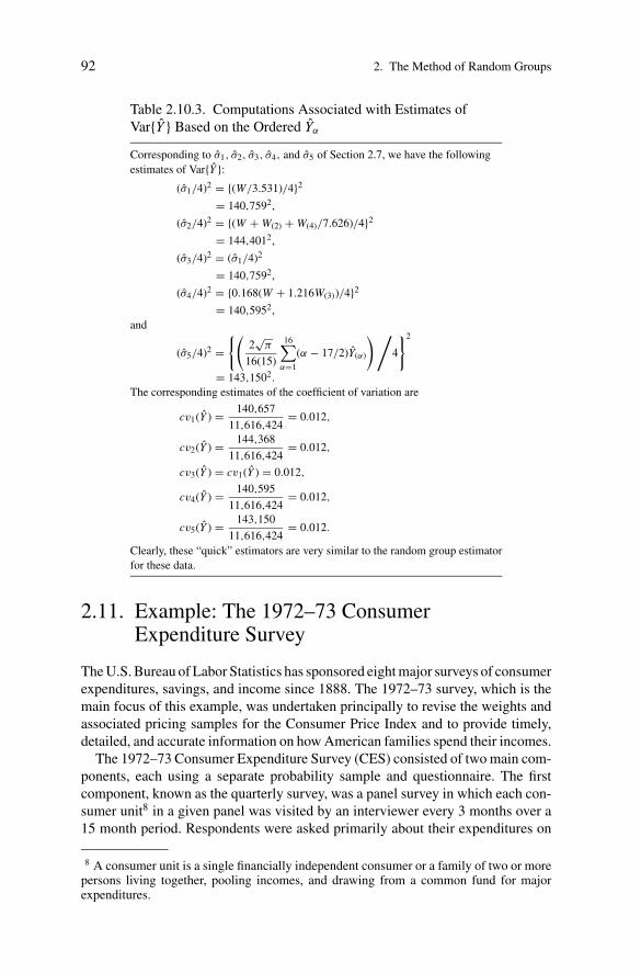
P1: OTE/SPH P2: OTE



Table 2.10.3. Computations Associated with Estimates ofVar{Y } Based on the Ordered Yα

Corresponding to σ1, σ2, σ3, σ4, and σ5 of Section 2.7, we have the following

estimates of Var{Y }:(σ1/4)2 = {(W/3.531)/4}2

= 140,7592,

(σ2/4)2 = {(W + W(2) + W(4)/7.626)/4}2

= 144,4012,

(σ3/4)2 = (σ1/4)2

= 140,7592,

(σ4/4)2 = {0.168(W + 1.216W(3))/4}2

= 140,5952,

and

(σ5/4)2 ={(

2√

π

16(15)

16∑α=1

(α − 17/2)Y(α)

) /4

}2

= 143,1502.

The corresponding estimates of the coefficient of variation are

cv1(Y ) = 140,657

11,616,424= 0.012,

cv2(Y ) = 144,368

11,616,424= 0.012,

cv3(Y ) = cv1(Y ) = 0.012,

cv4(Y ) = 140,595

11,616,424= 0.012,

cv5(Y ) = 143,150

11,616,424= 0.012.

Clearly, these “quick” estimators are very similar to the random group estimator

for these data.

2.11. Example: The 1972–73 ConsumerExpenditure Survey

The U.S. Bureau of Labor Statistics has sponsored eight major surveys of consumerexpenditures, savings, and income since 1888. The 1972–73 survey, which is themain focus of this example, was undertaken principally to revise the weights andassociated pricing samples for the Consumer Price Index and to provide timely,detailed, and accurate information on how American families spend their incomes.

The 1972–73 Consumer Expenditure Survey (CES) consisted of two main com-ponents, each using a separate probability sample and questionnaire. The firstcomponent, known as the quarterly survey, was a panel survey in which each con-sumer unit8 in a given panel was visited by an interviewer every 3 months over a15 month period. Respondents were asked primarily about their expenditures on

8 A consumer unit is a single financially independent consumer or a family of two or morepersons living together, pooling incomes, and drawing from a common fund for majorexpenditures.

P1: OTE/SPH P2: OTE


2.11. Example: The 1972–73 Consumer Expenditure Survey 93

major items; e.g., clothing, utilities, appliances, motor vehicles, real estate, andinsurance. The second component of CES was the diary survey, in which diarieswere completed at home by the respondents. This survey was intended to obtainexpenditure data on food, household supplies, personal care products, nonprescrip-tion drugs, and other small items not included in the quarterly survey.

To simplify the presentation, this example will be concerned only with the quar-terly survey. The sampling design, estimation procedure, and variance estimationprocedure for the diary survey were similar to those of the quarterly survey.

The quarterly survey employed a multistage, self-weighting sampling design.Its principal features included the following:

(1) The 1924 primary sampling units (PSU) defined for the Census Bureau’s Cur-rent Population Survey (see Hanson (1978)) were grouped into 216 strataon the basis of percent non-White and degree of urbanization. Fifty-four ofthese strata contained only one PSU (thus designated self-representing PSUs),while the remaining 162 strata contained two or more PSUs (thus designatednonself-representing PSUs).

(2) From each of the 162 strata, one PSU was selected using a controlled se-lection scheme. This scheme controlled on the number of SMSAs (StandardMetropolitan Statistical Area) from each of two size classes and on the ex-pected number of nonself-representing PSUs in each state.

(3) Within each selected PSU, a self-weighting sample of three types of units wasselected:(a) housing units that existed at the time of the 1970 Census,(b) certain types of group quarters,(c) building permits representing new construction since 1970.For simplicity this example will only describe the sampling of types (a) and (b)units. The sampling frame for types (a) and (b) units was the 20% sample ofhouseholds in the 1970 Decennial Census that received the census long form.

(4) Subsampling of types (a) and (b) units was performed independently in eachnonself-representing PSU. Existing housing units were assigned a samplingcode between 1 and 54 according to Table 2.11.1. Each group quarters personwas assigned sampling code 55. All types (a) and (b) units in each PSU werethen arranged into the following order,(a) sampling code,(b) state,(c) county,(d) census enumeration district (ED).For each PSU, a single random start was generated and a systematic sampleof housing units (HU) and group quarters persons was selected.

(5) All consumer units in selected housing units were taken into the sample.(6) A panel number between 1 and 3 was systematically assigned to each selected

HU and group quarters person in a modulo 3 fashion.(7) In self-representing PSUs, the sampling of types (a) and (b) units occurred as

in the nonself-representing PSUs. In self-representing PSUs, the selected unitswere then assigned to 15 random groups based on the order of the systematic

P1: OTE/SPH P2: OTE



Table 2.11.1. Sampling Codes for Housing Units for Within PSU Sampling

Rent or Value Owner Family Size Renter Family Size

Rent Value 1 2 3 4 5 + 1 2 3 4 5 +$0–$49 $0–$9,999 1 4 5 8 9 2 3 6 7 10

$50–$69 $10,000–$14,999 20 17 16 13 12 19 18 15 14 11

$70–$99 $15,000–$19,999 21 24 25 28 29 22 23 26 27 30

$100–$149 $20,000–$24,999 40 37 36 33 32 39 38 35 34 31

$150 + $25,000 + 41 44 45 48 49 42 43 46 47 50

51: Low Value Vacants (rent under $80 or value under $15,000)

52: Medium Value Vacants (rent of $80–$119 or value of $15,000–$24,999)

53: High Value Vacants (rent over $120 or value over $25,000)

54: Residual Vacants (those not for sale or rent).

selection. A random integer, α∗, between 1 and 15 was generated, and the firstunit selected was assigned to group α∗, the second to group α∗ + 1, and soforth in a modulo 15 fashion.

(8) Finally, the sample was divided in half, and one half was enumerated betweenJanuary 1972 and March 1973 and the second half between January 1973 andMarch 1974. Thirty of the original 54 self-representing PSUs were retainedin the sample for both years, but the subsample in each of these PSUs wasrandomly halved. The remaining 24 original self-representing PSUs and theoriginal nonself-representing PSUs were paired according to stratum size.Then, one PSU from each pair was assigned to 1972 and the other to 1973. Thisstep was not included in the original specification of the CES sampling design.It was instituted later when budgetary limitations necessitated extending thesample over two fiscal years instead of over one year, as originally specified.

The estimator of the total used in the quarterly survey was of the form

Y =∑i∈s

Wi Yi , (2.11.1)

where Yi is the value of the i-th consumer unit (CU) and Wi denotes the correspon-ding weight. The CU weights were generated by the following seven-step process:

(1) The base weight was the reciprocal of the inclusion probability.(2) A so-called duplication control factor9 was applied to the basic weight of

certain CUs selected in the new construction sample and existing CUs in twosmall PSUs.

(3) The weight resulting from step 2 was multiplied by a noninterview adjustmentfactor that was calculated for each of 106 noninterview cells within each offour geographical regions.

(4) First-stage ratio factors were then applied to the weights of all CUs in thenonself-representing PSUs. This factor was computed for ten race-residence

9 In a few cases, CUs were subsampled in large housing units. The duplication control factorsimply adjusted the weight to include the conditional probability due to subsampling.

P1: OTE/SPH P2: OTE



cells in each of the four geographic regions and took the form∑h

(1970 Census total for stratum h)∑h

(Sample PSU in stratum h)/πh,

where πh is the inclusion probability associated with the selected PSU instratum h and the summation is taken over all strata in the region. Thus, theweight resulting from step 3 for a given CU was multiplied by the factorappropriate for the region and race-residence cell corresponding to the CU.

(5) To adjust for noninterviewed CUs in multi-CU households, a multi-CU factorwas applied to the weight resulting from step 4.

(6) Next, a second-stage ratio factor was applied to each person 14 years old andover in each CU. This was computed for 68 age-sex-race cells and took theform

Independent population count of an age-sex-race cell

Sample estimate of the population of an age-sex-race cell,

where the independent population counts were obtained from the CensusBureau.

(7) Until the assignment of the second-stage ratio factor, all persons in a CU had thesame weight. But after the second-stage factor was applied, unequal weightswere possible. To assign a final weight to a CU, a so-called principal personprocedure10 was employed.

For a comprehensive discussion of the CES and its sample design and estima-tion schemes, see U.S. Department of Labor (1978). Here we have only attemptedto provide the minimal detail needed to understand the CES variance estimators.The description provided above suggests a complex sampling design and estima-tion scheme. The ensuing development shows the considerable simplification invariance estimation that results from the random group method.

In the CES, estimated totals and their associated variance estimates were com-puted separately for the self-representing (SR) and nonself-representing (NSR)PSUs. We begin by discussing the estimation for the SR PSUs. Subsequently, wediscuss the estimation for the NSR PSUs and the combined estimates over bothSR and NSR PSUs.

The variance due to subsampling within the SR PSUs was estimated in thefollowing fashion:

(1) The 30 SR PSUs were grouped into 15 clusters of one or more PSUs forpurposes of variance estimation.

10 Expenditure data were tabulated in the CES by designating a “principal person” andassigning that person’s weight to the CU. This was done because the second-stage ratiofactor applied to persons, not CUs. Since expenditure data were to be based on CUs, therewas a need to assign each CU a unique weight.

P1: OTE/SPH P2: OTE



(2) For each cluster, 15 random group totals were computed according to therelation

Y1cα =∑

i

15Wcαi Ycαi ,

where Ycαi denotes the value of the i-th CU in the α-th random group andc-th cluster and Wcαi denotes the corresponding weight as determined by theseven-step procedure defined above. Y1cα is the estimator in (2.11.1), wherethe summation has been taken only over units in the α-th random group andc-th cluster. The Wcαi are the parent sample weights, and the 15 Wcαi are theappropriate weights for a given random group.

(3) Cluster totals and variances were estimated by

Y1c =15∑

α=1

Y1cα/15

and

v(Y1c) = 1

15(14)

15∑α=1

(Y1cα − Y1c)2,

respectively.(4) Totals and variances over all SR PSUs were estimated by

Y1 =15∑c

Y1c

and

v(Y1) =15∑c

v(Y1c),

respectively.

The total variance (between plus within components) due to the sampling ofand within the NSR PSUs was estimated using the random group and collapsedstratum techniques.

(1) The 93 strata were collapsed into 43 groups, 36 of which contained two strataand seven of which contained three strata.

(2) For each NSR PSU, a weighted total was computed according to the relation

Y2gh =∑

i

Wghi Yghi ,

where Yghi denotes the value of the i-th CU in the h-th PSU in group g and Wghi

denotes the corresponding weight as determined by the seven-step proceduredefined earlier. Y2gh is the estimator in (2.11.1), where the summation has beentaken only over units in the h-th PSU in the g-th group. The Wghi are the fullsample weights. Thus Y2gh is an estimator of the total in the (g, h)-th stratum.

(3) Totals and variances over all NSR PSUs were estimated by

Y2 =43∑g

Y2g =43∑g

Lg∑h

Y2gh

P1: OTE/SPH P2: OTE



and

v(Y2) =36∑

g=1

22∑

h=1

(Y2gh − PghY2g)2

+43∑

g=37

3

2

3∑h=1

(Y2gh − PghY2g)2,

where Pgh is the proportion of the population in the g-th group living in the h-thstratum. Observe that v(Y2) is a collapsed stratum estimator. The factors Pgh

are analogous to the Agh/Ag in equation (2.5.7). Population is an appropriatefactor here because it should be well-correlated with the expenditure items ofinterest in the CES.

Finally, totals and variances over both SR and NSR PSUs were estimated by

Y = Y1 + Y2 (2.11.2)

and

v(Y ) = v(Y1) + v(Y2),

respectively. The variance of Y is the sum of the variances of Y1 and Y2 becausesampling was performed independently in the SR and NSR strata.

Before presenting some specific variance estimates, two aspects of the esti-mation procedure require special discussion. First, the application of the randomgroup method did not adhere strictly to the principles discussed in Sections 2.2 and2.4 of this chapter. Recall that the weights attached to the sample units includednonresponse adjustments and first- and second-stage ratio adjustments. All of theseadjustment factors were computed from the entire sample, whereas strict randomgroup principles would suggest computing these factors individually for each ran-dom group. The adopted procedure is clearly preferable from a computationalstandpoint, and it also can be justified in some cases by Taylor series arguments.Second, the collapsed stratum feature of the variance estimation procedure proba-bly tended to overstate the actual variance. As was shown in Section 2.5, such over-statement tends to occur when one unit is selected independently within each stra-tum. In the CES, however, primaries were sampled by a controlled selection proce-dure, and to the extent that this resulted in a lower true variance than an independentselection procedure, the overestimation of variance may have been aggravated.

The principal estimates derived from the quarterly survey included the totalnumber of CUs and the mean annual expenditure per CU for various expenditurecategories. The estimator of mean annual expenditure was of the ratio form, andits variance was estimated using a combination of random group and Taylor seriesmethodologies. For that reason, the discussion of variance estimation for meanannual expenditures will be deferred until Chapter 6 (see Section 6.8).

Estimation of the total number of CUs is described in Tables 2.11.2–2.11.5.Random group totals for the SR and NSR PSUs are presented in Tables 2.11.2 and2.11.3, respectively. The factors Pgh are given in Table 2.11.4. Both the SR andNSR variances are computed in Table 2.11.5.

P1: OTE/SPH P2: OTE


Tab

le2

.11

.2.

Ran

do

mG

rou

pT

ota

lsY

1cα

for

15

SR

PS

UC

lust

ers

for

the

Ch

arac

teri

stic

“Nu

mb

ero

fC

on

sum

erU

nit

s”

Ran

do

mG

rou

p

Clu

ster

12

34

56

78

910

11

12

13

14

15

14

08

,63

9.0

35

7,3

96

.04

06

,58

2.0

46

3,0

05

.04

27

,26

5.0

43

3,7

18

.03

16

,82

1.0

36

7,5

99

.04

65

,27

9.0

36

8,7

89

.03

12

,06

6.0

37

9,8

08

.03

82

,06

6.0

30

8,0

08

.03

10

,03

4.0

28

4,4

75

.56

5,9

30

.71

09

,24

0.0

11

5,3

05

.01

19

,15

8.0

54

,82

2.7

10

8,1

68

.01

31

,38

7.0

11

3,4

61

.01

47

,63

7.0

71

,46

2.7

11

1,2

32

.01

13

,08

5.0

11

3,6

32

.01

16

,21

1.0

39

0,7

31

.17

8,8

54

.11

01

,14

5.0

99

,78

6.3

69

,82

2.7

85

,44

8.8

11

9,9

23

.09

0,0

64

.08

3,7

36

.49

9,3

58

.46

8,4

73

.69

6,2

95

.31

14

,04

8.0

88

,35

7.6

92

,10

0.0

46

5,4

56

.78

2,4

99

.16

4,6

32

.75

5,3

32

.46

2,7

20

.25

6,8

97

.97

5,3

27

.14

6,5

51

.67

3,0

08

.55

9,2

97

.75

6,1

98

.87

2,1

27

.16

1,6

64

.25

6,3

34

.86

5,7

64

.3

58

3,5

25

.38

1,7

85

.17

3,2

53

.17

7,6

08

.75

8,8

87

.59

2,7

49

.95

9,0

08

.97

2,4

72

.19

3,0

13

.38

2,5

58

.86

4,4

00

.18

8,4

24

.07

3,7

46

.08

5,2

62

.39

5,2

49

.9

68

7,0

31

.87

7,7

88

.01

08

,04

3.0

90

,72

0.5

63

,49

7.7

85

,11

3.3

70

,37

8.6

99

,84

8.2

74

,70

4.6

10

8,0

67

.05

1,3

08

.88

3,7

27

.08

1,6

78

.48

7,6

35

.59

1,7

42

.5

76

5,7

41

.18

3,3

96

.65

7,4

53

.97

7,1

80

.57

2,4

51

.97

1,3

07

.48

5,1

04

.47

1,5

18

.88

4,4

60

.79

2,2

31

.58

0,0

08

.28

2,3

44

.57

4,6

16

.09

5,9

72

.36

8,9

59

.0

81

85

,62

3.0

15

6,1

94

.01

64

,00

3.0

17

4,1

97

.01

41

,76

2.0

15

4,7

99

.01

75

,70

2.0

12

2,7

18

.01

76

,83

8.0

20

0,0

17

.01

24

,95

2.0

19

2,5

07

.01

58

,45

7.0

18

1,0

52

.01

61

,94

7.0

97

5,6

39

.16

4,1

96

.39

3,4

21

.41

08

,32

1.0

10

0,9

72

.09

3,0

13

.99

5,7

22

.48

6,7

39

.61

36

,03

3.0

69

,89

3.2

91

,16

7.2

10

0,2

65

.09

6,1

95

.11

08

,93

0.0

10

0,1

51

.0

10

10

1,3

72

.09

0,6

63

.49

1,0

30

.57

9,9

64

.81

12

,67

7.0

86

,18

3.4

78

,26

5.5

93

,57

5.0

77

,85

1.6

78

,36

2.5

84

,92

6.5

12

1,2

52

.08

3,1

96

.47

9,6

38

.57

7,9

02

.5

11

90

,18

7.9

99

,52

8.5

81

,69

3.6

94

,27

8.5

11

3,1

66

.06

7,3

75

.59

1,1

08

.61

09

,07

7.0

61

,28

4.6

85

,51

6.7

78

,26

3.5

78

,88

7.1

10

1,2

57

.09

3,6

91

.79

9,2

27

.3

12

12

6,0

03

.01

08

,54

0.0

13

4,7

45

.01

42

,04

5.0

15

6,8

87

.01

21

,07

0.0

91

,08

5.9

10

2,8

99

.01

07

,93

3.0

13

5.4

42

.01

03

,74

7.0

12

1,2

09

.01

37

,17

9.0

12

6,8

90

.09

8,2

91

.6

13

18

7,6

73

.01

72

,83

8.0

18

2,2

23

.01

64

,62

9.0

15

7,8

16

.01

86

,88

0.0

18

8,2

80

.01

99

,17

2.0

16

4,6

40

.01

88

,26

1.0

17

1,6

94

.01

96

,74

7.0

18

6,8

55

.01

71

,84

4.0

21

5,7

60

.0

14

12

8,9

11

.09

8,1

33

.01

33

,03

2.0

11

6,2

59

.01

49

,56

3.0

10

1,2

64

.01

12

,74

6.0

11

2,1

80

.01

37

,85

7.0

10

4,2

27

.01

16

,84

8.0

11

4,1

50

.09

3,0

83

.51

13

,72

3.0

10

1,2

38

.0

15

12

3,4

50

.01

55

,27

8.0

12

9,7

59

.01

93

,34

7.0

14

4,4

12

.01

81

,26

0.0

14

6,8

56

.01

23

,34

6.0

17

8,6

17

.01

38

,64

1.0

12

4,4

11

.01

17

,42

4.0

15

1,3

47

.01

45

,66

6.0

12

5,5

46

.0

Sour

ce:

C.

Dip

po

,p

erso

nal

com

mu

nic

atio

n(1

97

7).

Not

e:A

llen

trie

sin

this

tab

lesh

ou

ldb

em

ult

ipli

edb

y1

5.

98

P1: OTE/SPH P2: OTE



Table 2.11.3. Estimated Totals Y2gh for 43 Collapsed Stratafor the Characteristic “Number of Consumer Units”

Stratum (h)

Group (g) 1 2 3

1 361,336 434,324

2 413,727 479,269

3 446,968 408,370

4 520,243 598,114

5 375,400 467,515

6 477,180 464,484

7 494,074 496,722

8 437,668 456,515

9 387,651 430,562

10 450,008 467,255

11 485,998 502,247

12 464,604 393,965

13 415,047 472,583

14 444,814 481,008

15 375,815 442,793

16 438,436 474,527

17 451,239 382,624

18 460,168 311,482

19 462,894 470,407

20 493,373 540,379

21 469,461 394,530

22 426,485 546,285

23 515,182 974,332

24 436,378 410,247

25 436,449 362,472

26 383,687 431,037

27 387,268 419,426

28 302,383 441,139

29 432,195 454,737

30 432,159 426,645

31 440,998 374,043

32 367,096 528,503

33 428,326 549,871

34 395,286 456,075

35 410,925 220,040

36 465,199 475,912

37 449,720 387,772 471,023

38 441,744 437,025 640,130

39 651,431 364,652 638,782

40 441,244 420,171 362,705

41 489,315 463,869 384,602

42 443,885 476,963 397,502

43 821,244 692,441 431,657

P1: OTE/SPH P2: OTE



Table 2.11.4. Factors Pgh Used in Computing the VarianceDue to Sampling in NSR Strata

Stratum (h)

Group (g) 1 2 3

1 0.486509 0.513491

2 0.485455 0.514545

3 0.496213 0.503787

4 0.438131 0.561869

5 0.493592 0.506408

6 0.505083 0.494917

7 0.503599 0.496401

8 0.499901 0.500099

9 0.501436 0.498564

10 0.507520 0.492480

11 0.503276 0.496724

12 0.500381 0.499619

13 0.501817 0.498183

14 0.501071 0.498929

15 0.500474 0.499526

16 0.489670 0.510330

17 0.495551 0.504449

18 0.500350 0.499650

19 0.496320 0.503680

20 0.497922 0.502078

21 0.498676 0.501324

22 0.475579 0.524421

23 0.459717 0.540283

24 0.495257 0.505743

25 0.499968 0.500032

26 0.499178 0.500822

27 0.498887 0.501113

28 0.497341 0.502659

29 0.499085 0.500915

30 0.499191 0.500809

31 0.498829 0.501171

32 0.484498 0.515502

33 0.510007 0.489993

34 0.532363 0.467637

35 0.471407 0.528593

36 0.486899 0.513101

37 0.318160 0.338869 0.342971

38 0.313766 0.323784 0.362450

39 0.409747 0.312005 0.278248

40 0.337979 0.333625 0.328396

41 0.325368 0.333347 0.341285

42 0.331581 0.334400 0.334019

43 0.414992 0.332518 0.252491

P1: OTE/SPH P2: OTE


2.12. Example: The 1972 Commodity Transportation Survey 101

Table 2.11.5. Estimated Totals and Variances for Both SR and NSR PSUs

Y1cα is the element in the c-th row, α-th column of Table 2.11.2. Thus, the

estimated total and variance for the SR PSUs are

Y1 =15∑c

Y1c =15∑c

15∑α

Y1cα/15 = 28.2549 · 106

and

v(Y1) =15∑c

v(Y1c) =15∑c

1

15(14)

15∑α

(Y1cα − Y1c)2 = 10.2793 · 1010,

respectively.

Y2gh and Pgh are the elements in the g-th row, h-th column of Tables 2.11.3 and

2.11.4, respectively. Thus, the estimated total and variance for the NSR PSUs are

Y2 =43∑g

Y2g =43∑g

Lg∑h

Y2gh = 42.5344 · 106

and

v(Y2) =36∑

g=1

22∑

h=1

(Y2gh − PghY2g)2

+43∑

g=37

(3/2)3∑

h=1

(Y2gh − PghY2g)2

= 46.5747 · 1010,

respectively.

The estimated total and variance over both SR and NSR PSUs are

Y = Y1 + Y2 = 70.7893 · 106

and

v(Y ) = v(Y1) + v(Y2) = 56.8540 · 1010.

2.12. Example: The 1972 CommodityTransportation Survey

The 1972 Commodity Transportation Survey was a part of the 1972 U.S. Censusof Transportation. Prime objectives of the survey included the measurement ofthe transportation and geographic distribution of commodities shipped beyond thelocal area by manufacturing establishments in the United States.

This example is limited to the Shipper Survey, which was the major componentof the Commodity Transportation Survey program. The frame for the ShipperSurvey was derived from the 1972 U.S. Census of Manufacturers, and consisted ofall manufacturing establishments in the United States with 20 or more employees,there being approximately 100,000 in number. The Mail Summary Data Survey, aminor component of the Commodity Transportation Survey program, covered themanufacturing plants with less than 20 employees.

Key features of the sampling design and estimation procedure for the ShipperSurvey included the following:

P1: OTE/SPH P2: OTE



Table 2.12.1. Allocation of the Sample for the Shipper Survey

Number of Selected PlantsTonnage Shipper

Division Classes Certainty Noncertainty Total

1 1 81 40 121

2 5 459 696 1,155

3 5 354 578 932

4 4 339 541 880

5 13 1,242 1,045 2,287

6 12 771 866 1,637

7 15 880 1,318 2,198

8 13 675 1,102 1,777

9 17 585 1,348 1,933

Total 85 5,386 7,534 12,920

Source: Wright (1973).

(i) Using the Federal Reserve Board’s Index of Industrial Production, manufac-turing plants were divided into 85 shipper classes. Each class was composedof similar SIC (Standard Industrial Classification) codes.

(ii) Each shipper class was then assigned to one of nine tonnage divisions basedon total tons shipped. Each tonnage division comprised a separate samplingstratum.

(iii) Within a tonnage division, manufacturing plants were ordered by shipperclass, by state, and by SIC code.

(iv) Each plant was assigned an expected tonnage rating on the basis of theplant’s total employment size.

(v) Based on the expected tonnage rating, a certainty cutoff was specifiedwithin each tonnage division. All plants with a rating greater than the cutoffwere included in the sample with probability one.

(vi) An unequal probability, single-start systematic sample of plants was se-lected independently from within the noncertainty portion of each tonnagedivision. The selection was with probability proportional to expectedtonnage rating. The sample sizes are given in Table 2.12.1.

(vii) Within each selected manufacturing plant, an equal probability sample ofbills of lading was selected. The filing system for shipping documents variesfrom plant to plant, but often the papers are filed by a serial number. If so,a single-start systematic sample of bills of lading was selected (see Table2.12.2 for subsampling rates). If not, then a slightly different samplingprocedure was employed. The alternative subsampling procedures arenot of critical importance for this example and thus are not describedhere.

P1: OTE/SPH P2: OTE



Table 2.12.2. Subsampling Rates for ShippingDocuments Filed in Serial Number Order

Number of Documents in File Sampling Rate

0–199 1/1

200–399 1/2

400–999 1/4

1,000–1,999 1/10

2,000–3,999 1/20

4,000–9,999 1/40

10,000–19,999 1/100

20,000–39,999 1/200

40,000–79,999 1/400

80,000–99,999 1/500

(viii) Population totals were estimated using the Horvitz–Thompson estimator

Y = Y0 + Y1 + Y2

=∑

i

∑j

Y0i j +∑

i

∑j

Y1i j/π1i j +∑

i

∑j

Y2i j/π2i j ,

where Yci j denotes the value of the j-th document in the i-th plantand πci j denotes the associated inclusion probability. The c subscriptdenotes

c = 0 document selected at the rate 1/1from within a certainty plant,

c = 1 document selected at a rate < 1/1from within a certainty plant,

c = 2 document selected from a,noncertainty plant.

The variance of Y was estimated using the random group method. Plants wereassigned to k = 20 random groups in the following fashion:

(ix) All noncertainty plants were placed in the following order:

tonnage division,shipper class,state,plant ID.

(x) A random integer between 1 and 20 was generated, say α∗. The first plantwas then assigned to random group (RG) α∗, the second to RG α∗ + 1, andso forth in a modulo 20 fashion.

P1: OTE/SPH P2: OTE



(xi) All selected second-stage units (i.e., bills of lading) within a selected non-certainty plant were assigned to the same RG as the plant.

(xii) All second-stage units selected at the rate 1/1 within certainty plants wereexcluded from the 20 RGs.

(xiii) Second-stage units selected at a rate < 1/1 within certainty plants wereplaced in the following order:

tonnage division,shipper class,state,plant ID.

(xiv) The second-stage units in (xiii) were assigned to the k = 20 random groupsin the systematic fashion described in (x).

The random group estimator of Var{Y } is prepared by estimating the variancefor certainty plants and noncertainty plants separately. The two estimates are thensummed to give the estimate of the total sampling variance. The random groupestimator for either the certainty (c = 1) or noncertainty plants (c = 2) is definedby

v(Yc) = 1

20(19)

20∑α=1

(Ycα − Yc)2, (2.12.1)

where c = 1, 2,

Ycα =∑

(c,i, j)∈s(α)

Yci j (20/πci j ),

∑(c,i, j)∈s(α) denotes a sum over units in the α-th random group, and the

πci j/20 are the inclusion probabilities associated with the individual randomgroups.

Table 2.12.3 presents some typical estimates and their estimated coefficients ofvariation (CV) from the Shipper Survey. These estimates include the contributionfrom both certainty and noncertainty plants.

To illustrate the variance computations, Table 2.12.4 gives the random group to-tals for the characteristic “U.S. total shipments over all commodities.” The estimateof the total tons shipped is

Y = Y0 + Y1 + Y2

= Y0 +20∑

α=1

Y1α/20 +20∑

α=1

Y2α/20

= 42.662 · 106 + 236.873 · 106 + 517.464 · 106

= 796.99 · 106,

where Y0 is the total of certainty shipments associated with certainty plants.

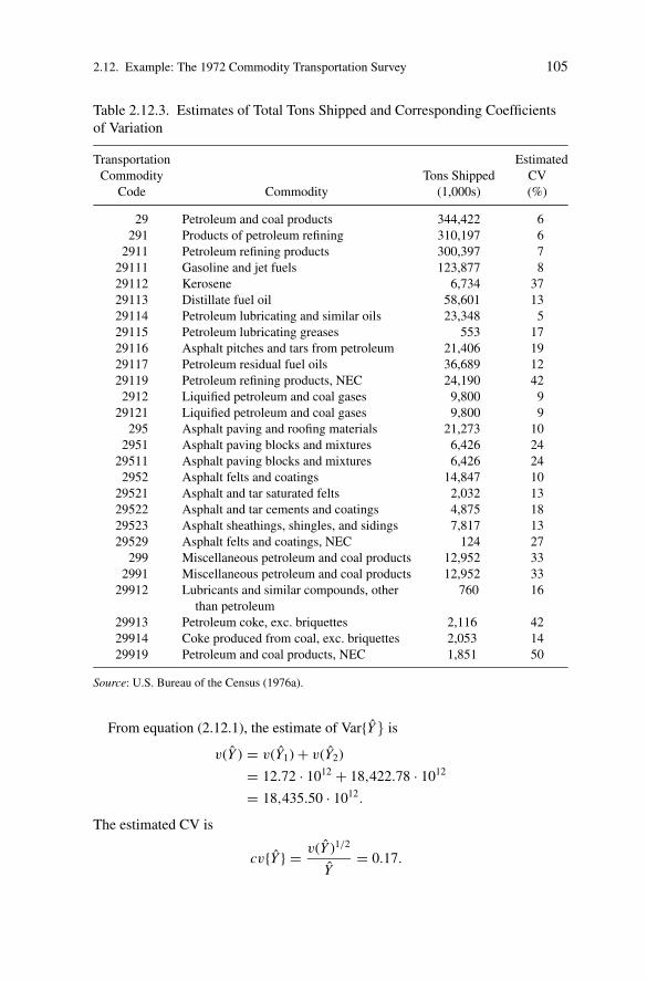
P1: OTE/SPH P2: OTE



Table 2.12.3. Estimates of Total Tons Shipped and Corresponding Coefficientsof Variation

Transportation Estimated

Commodity Tons Shipped CV

Code Commodity (1,000s) (%)

29 Petroleum and coal products 344,422 6

291 Products of petroleum refining 310,197 6

2911 Petroleum refining products 300,397 7

29111 Gasoline and jet fuels 123,877 8

29112 Kerosene 6,734 37

29113 Distillate fuel oil 58,601 13

29114 Petroleum lubricating and similar oils 23,348 5

29115 Petroleum lubricating greases 553 17

29116 Asphalt pitches and tars from petroleum 21,406 19

29117 Petroleum residual fuel oils 36,689 12

29119 Petroleum refining products, NEC 24,190 42

2912 Liquified petroleum and coal gases 9,800 9

29121 Liquified petroleum and coal gases 9,800 9

295 Asphalt paving and roofing materials 21,273 10

2951 Asphalt paving blocks and mixtures 6,426 24

29511 Asphalt paving blocks and mixtures 6,426 24

2952 Asphalt felts and coatings 14,847 10

29521 Asphalt and tar saturated felts 2,032 13

29522 Asphalt and tar cements and coatings 4,875 18

29523 Asphalt sheathings, shingles, and sidings 7,817 13

29529 Asphalt felts and coatings, NEC 124 27

299 Miscellaneous petroleum and coal products 12,952 33

2991 Miscellaneous petroleum and coal products 12,952 33

29912 Lubricants and similar compounds, other 760 16

than petroleum

29913 Petroleum coke, exc. briquettes 2,116 42

29914 Coke produced from coal, exc. briquettes 2,053 14

29919 Petroleum and coal products, NEC 1,851 50

Source: U.S. Bureau of the Census (1976a).

From equation (2.12.1), the estimate of Var{Y} is

v ˆ(Y ) = v(Y1) + v(Y2)

= 12.72 · 1012 + 18,422.78 · 1012

= 18,435.50 · 1012.

The estimated CV is

cv{Y } = v(Y )1/2

Y= 0.17.

P1: OTE/SPH P2: OTE



Tab

le2

.12

.4.

Ran

do

mG

rou

pT

ota

lsfo

rth

eC

har

acte

rist

ic“U

.S.

To

tal

Sh

ipm

ents

Over

All

Co

mm

od

itie

s”

To

tal

Cer

tain

tyN

on

cert

ain

ty

Ran

do

mE

stim

ated

Est

imat

edE

stim

ated

Gro

up

Do

cum

ents

aT

on

sS

hip

ped

Do

cum

ents

To

ns

Sh

ipp

edD

ocu

men

tsT

on

sS

hip

ped

14

77

71

,29

3,2

32

,12

01

88

12

16

,17

8,5

80

28

96

1,0

77

,05

3,5

40

24

95

04

26

,48

4,1

60

18

92

27

4,2

75

,90

03

05

81

52

,20

8,2

60

34

51

63

,14

2,5

17

,88

01

88

02

35

,32

2,3

00

26

36

2,9

07

,19

5,5

80

44

66

95

09

,36

6,1

00

18

90

24

1,4

08

,26

02

77

92

67

,95

7,8

40

54

62

44

89

,69

0,3

20

18

89

23

3,9

60

,94

02

73

52

55

,72

9,4

00

64

57

15

26

,58

1,3

60

18

78

22

8,8

75

,38

02

69

32

97

,70

5,9

80

74

74

06

46

,95

7,0

40

18

85

23

1,8

06

,94

02

85

54

15

,15

0,1

00

85

13

74

67

,64

8,5

00

18

81

21

2,2

05

,22

03

25

62

55

,44

3,3

00

94

66

97

73

,25

7,4

00

18

77

24

0,2

78

,44

02

79

25

32

,97

8,9

60

10

51

18

51

4,7

19

,50

01

88

02

24

,67

6,1

40

32

38

29

0,0

43

,36

0

11

46

37

56

9,1

37

,60

01

88

12

32

,15

8,7

60

27

56

33

6,9

78

,84

0

12

46

88

1,0

54

,60

5,1

00

18

77

21

4,5

50

,74

02

81

18

40

,05

4,3

60

13

47

19

67

9,2

91

,88

01

88

02

45

,13

8,2

40

28

39

43

4,1

53

,64

0

14

46

67

51

3,1

00

,86

01

89

02

61

,39

4,8

40

27

77

25

1,7

06

,02

0

15

46

14

52

5,3

85

,74

01

89

22

34

,41

9,4

40

27

22

29

0,9

66

,30

0

16

51

27

40

4,8

42

,34

01

90

32

49

,83

9,5

40

32

24

15

5,0

02

,80

0

17

47

86

50

8,0

47

,30

01

88

42

45

,80

7,8

60

29

02

26

2,2

39

,42

0

18

49

59

57

4,5

08

,14

01

89

62

20

,53

6,2

40

30

63

35

3,9

71

,90

0

19

48

27

86

9,5

75

,52

01

88

52

37

,55

3,9

60

29

42

63

2,0

21

,56

0

20

47

38

59

7,7

70

,90

01

89

02

57

,06

9,8

60

28

48

34

0,7

01

,02

0

Cer

tain

tyb

74

10

42

,66

1,7

91

74

10

42

,66

1,7

91

00

aU

nw

eighte

dnum

ber

of

seco

nd-s

tage

unit

s.b

Tota

lof

cert

ainty

seco

nd-s

tage

unit

sas

soci

ated

wit

hce

rtai

nty

pla

nts

.