The Masking of Declining Manufacturing Employment by the Housing Bubble

Kerwin Kofi Charles, Erik Hurst, and Matthew J. Notowidigdo

Kerwin Kofi Charles is Edwin and Betty L. Bergman Professor, University of Chicago Harris School of Public Policy, Chicago, Illinois. Erik Hurst is the V. Duane Rath Professor of Economics and the John E. Jeuck Faculty Fellow, University of Chicago Booth School of Business, Chicago, Illinois. Matthew J. Notowidigdo is Associate Professor of Economics, Northwestern University, Evanston, Illinois. All three authors are Research Associates, National Bureau of Economic Research, Cambridge, Massachusetts. Their email addresses are kerwin.charles@gmail.com, erik.hurst@chicagobooth.edu, and noto@northwestern.edu. * JEL codes: J21, E24, E32, R23.

1

The employment-to-population ratio among prime-aged adults aged 25-54 has fallen

substantially since 2000. Hall (2014), one of many authors to have commented on the large decline,

describes it as the defining feature of the labor market since 2000.1 Similarly, Acemoglu et al. (2016)

call the employment decline of the 2000s the “Great U.S. Employment Sag.” The magnitude of the

fall in employment and its distribution across the population can be seen in Figure 1. This figure

shows the employment rate from 1980 to 2015, separately by gender and education level, using annual

data from the March Current Population Survey (CPS). Most of the reduction in the employment rate

since about 2000 has come from those without a four-year college degree, who we refer to as “non-

college” throughout this paper. The employment rate for prime-aged, non-college men hovered

around 85 percent from 1980 to 2000, but in 2014 was only 79 percent, fully 6 percentage points

below the 2000 level. The employment rates for prime-aged, non-college women fell from roughly

70 percent in the late 1990s to 64 percent in 2015, also a decline of about 6 percentage points relative

to the 2000 level. These large and seemingly persistent reductions in employment among the less-

educated over the course of the 2000s were much larger than those for both prime-aged men and

women with four-year college degrees, whose employment rates fell by only about 2 percentage points

between 2000 and 2014.

The explanations proposed for the decline in the employment-to-population ratio have been

of two broad types. Focusing on the fact that the employment rate decline was especially sharp from

2007-2010, during and immediately after the Great Recession, one set of explanations emphasizes

cyclical factors associated with the recession, including temporary declines in labor demand, economic

and policy uncertainty, “mismatch” between unemployed workers and jobs, and the availability of

unemployment insurance for extended periods. The second set of explanations focuses on the role

of longer-run structural factors, the potential importance of which is suggested by the reduction in

the employment rate even before the start of the Great Recession began, and the persistently low

employment-to-population rates for low-skilled workers years after its official end. Structural

explanations focus on long-term secular trends, such as the falling demand for routine tasks

1 Others to comment on the decline include Hall (2011), Moffit (2012), and Davis and Haltiwanger (2014).

2

performed by workers in many manufacturing jobs. However, if structural factors indeed explain

much of the decline in employment since 2000, it is not immediately clear why the effect of these

long-term factors should have been so modest from 2000 to 2007, only to appear with sudden and

pronounced effect during the Great Recession.

In this paper, we argue that while the decline in manufacturing and the consequent reduction in

demand for less-educated workers put downward pressure on their employment rates in the pre-

recession 2000-2006 period, the increased demand for less-educated workers because of the housing

boom was simultaneously pushing their employment rates upwards (Charles, Hurst, and Notowidigdo

2013, 2015). For a few years, the housing boom served to “mask” the labor market effects of

manufacturing decline for less-educated workers. When the housing market collapsed in 2007, there

was a large, immediate decline in employment among these workers, who faced not only the sudden

disappearance of jobs related to the housing boom, but also the fact that manufacturing’s steady

decline during the early 2000s left them with many fewer opportunities in that sector than had existed

at the start of the decade.

We begin with a short overview of various cyclical and structural arguments about the decline in

the employment-to-population ratio. We then present several different pieces of evidence which

support our hypothesis that the masking and unmasking of manufacturing decline by the housing

boom and bust play an important role in changes in the employment rate since 2000.

The evidence we present in support of this argument includes aggregate time series results; local labor

market evidence which exploits the large variation in the size of manufacturing decline and in the size

of the housing boom and bust across different metropolitan areas in the United States; and individual-

level evidence using data about the re-employment rates of displaced manufacturing workers in the

Displaced Workers Survey. Our focus throughout is on prime-aged, non-college men. However, in

the conclusion we briefly discuss employment masking for prime-aged, non-college women, as well.

Our conclusion also discusses why the distinction between cyclical and structural forces is important

for policymaking.

3

Reviewing Cyclical and Structural Explanations of Employment Rate Changes Since 2000

Most of the decline in the employment-to-population ratio for lower-skilled workers since 2000

occurred during the Great Recession, as shown in Figure 1. Perhaps because of this, several recent

papers seeking to understand employment changes have focused on “cyclical” explanations.

One strand of this work studies the role of the negative shocks to household and bank balance

sheets that arose from the recession. Using cross-region data, Mian and Sufi (2014) find that local

areas that experienced larger declines in household net worth had larger reductions in employment in

non-tradable sectors during the 2007-2009 period. Chodorow-Reich (2014) links the decline in

employment to disruptions in the banking sector, by showing that firms that had pre-recession

relationships with distressed banks were much less likely to secure credit during the recession, and

were much more likely to shed employment during 2007-2009.2 Mondragon (2015) estimates the

effect of local credit supply shocks on employment and finds a large effect.3 Also broadly related to

this area of research is Giroud and Mueller (2015), who find that high firm leverage before the start

of the Great Recession also contributed to large employment losses during the recession.

Several other papers in this literature assess other cyclical factors that were likely changed because

of the recession, including increased economic and policy uncertainty, increases in sectoral and spatial

mismatch, and changes in the duration and generosity of unemployment benefits and other transfer

programs. Baker, Bloom, and Davis (2013) show that measures of aggregate uncertainty were high

during the Great Recession relative to historical levels, and argue that this increased uncertainty can

account for some of the decline in the employment rate. Similar explanations are also found in

Fernandez-Villaverde et al. (2013). Sahin, Song, Topa, and Violante (2014) examine the extent to

which search frictions that affect the ease with which workers can move between occupations and

2 A large theoretical literature examines the role of tightening borrowing constraints on households and firms and how that translates into declining aggregate employment: for example, see Eggerson and Krugman (2012) and Guerrieri and Lorenzoni (2015). 3 Greenstone et al. (2015) also examine the relationship between local credit supply shocks to local banks and local employment outcomes. They show that while credit supply shocks do reduce credit to small firms, the employment losses of small firms have little effect on local employment rates.

4

locations may have increased the unemployment rate and reduced the employment rate. Their results

suggest that these mismatch forces may explain as much as one-third of the rise in the unemployment

rate between 2007 and 2010, with the effect diminishing by 2012.

The growing literature relating the decline in aggregate employment to the expansion of

unemployment benefits during the Great Recession has come to mixed conclusions. Rothstein (2013)

and Farber and Valletta (2013) find that although unemployment benefit extension may have propped

up the unemployment rate by delaying exits from the labor force, benefit extension did not have

much of an effect on the employment rate. However, both Johnston and Mas (2015) and Hagerdorn

et al. (2015) find larger effects of unemployment benefit extensions. Additionally, Mulligan (2012)

discusses how broader policy changes that occurred during the recession – such as the expansion of

the Supplemental Nutritional Assistance Program (often known as Food Stamps) – could have

discouraged individual labor supply and thus reduced the employment rate.

Finally, another important program that could have had an important effect on aggregate

employment during the recession and thereafter is Social Security Disability Insurance (SSDI). Even

before the Great Recession, there were staggering increases in enrollment, due both to reduced

screening stringency and higher demand for the partial wage insurance provided by the program

(Autor and Duggan 2006). Although there were no significant changes to the program during the

Great Recession, research has documented a strong link between labor market conditions and SSDI

application rates (Autor and Duggan 2003; Sloane 2015), and strong effects of SSDI on both

employment and earnings (Maestas et al. 2013). Sloane (2015) documents large increases in disability

rates between 2007 and 2011 in local markets with large increases in unemployment rates during the

Great Recession. Given that disability tends to be persistent, this could explain some of the low

employment to population rates after the recession. Her estimates, however, suggests such effects are

modest. Additionally, unlike UI and many other social insurance programs, there are often large

waiting times to get onto SSDI, which means that denied SSDI applicants typically search for work

after long periods of detachment from the labor market. The delay in processing applications appears

to generate duration dependence in non-employment, making it harder for rejected applicants to

5

return to the labor (Autor et al. 2015).4 As a result, the large number of rejected SSDI applicants

during the Great Recession may experience lower employment rates in the longer-run (Maestas et al.

2015).

While the preceding papers seem to explain a meaningful share of the employment changes

observed over the course of the Great Recession, a problem for the notion that cyclical factors are

the main explanation for the full pattern of observed employment changes since 2000 is that cyclical

factors cannot readily explain the persistence of reduced employment among prime-age lower-skilled

individuals – the fact that rates have remained low long after the impact of cyclical factors from the

recession should have ended. Despite growing evidence of market normalization in the years since

the end of the Great Recession – stabilization of housing prices, favorable lending conditions, declines

in aggregate uncertainty, return of labor market mismatch to pre-recessionary levels, and the cessation

of extended unemployment benefits – the employment rate remains significantly below pre-

recessionary levels.

Alongside the literature studying cyclical factors, another literature has emerged studying the role

of structural factors in explaining recent changes in employment. How long-term changes in

underlying demographics, such as the ageing of the population, have contributed to the decline in

labor force participation has been the focus one strand of research (see, e.g., Aaronson et al. 2015).

On the whole, result from this work indicate that demographic factors explain a portion of the overall

decline in employment and labor force participation. Our work focuses throughout on the population

of prime-aged, non-college men, so the declines we document and attempt to explain cannot be

accounted for by changes in demographics, and must be due to other factors. The focus on these

other factors complements existing work studying demographics.

Another strand of the work studying longer-term structural factors has linked declining demand

for routine tasks (Autor et al. 2003) and job polarization (Autor and Dorn 2013) to declining

4 For simplicity, this section focuses on explanations of changes in employment during 2000s that can be readily categorized into either cyclical or structural explanations. However, factors such as duration dependence belong to a class of explanations that suggest important interactions between the two. For example, Kroft et al. (2016) calibrate a search and matching model to show that the low job finding rate in the aftermath of the Great Recession may partly be due to duration dependence in unemployment. As a result, the sharp decline in vacancies generated an increase in long-term unemployment and – through duration dependence in unemployment – reduced both the overall job-finding rate and aggregate employment.

6

employment rates for less-educated workers during the 2000s. Autor, Dorn and Hanson (2013),

Charles, Hurst, and Notowidigdo (2013), and Acemoglu et al. (2016) all discuss how the decline in

manufacturing during the 2000s depressed employment rates for less-educated workers. International

trade appears to account for some of the decline in manufacturing employment. Autor, Dorn, and

Hanson (2013) provide local labor markets evidence that increased important competition from

increased trade with China reduced manufacturing employment during the 1990s and 2000s.

Similarly, Pierce and Schott (2016) provide evidence that the “surprisingly swift” decline of

manufacturing during the 2000s is linked to changes in trade policy that eliminated potential tariff

increases for Chinese imports. Consistent with their interpretation of the role of changes in trade

policy, there is a clear divergence in manufacturing employment trends between the U.S. and EU

following this policy change.

These papers suggest an important role for structural factors in understanding pattern of

employment changes since 2000. However, it is not clear how these relatively slow-moving structural

shifts could explain the sudden reduction in employment rates after 2008. Furthermore, since any

structural forces affecting employment likely operated steadily throughout the 2000s, one would have

expected their influence to reduce employment substantially before the recession. Yet, employment

rates in the early 2000s declined only modestly.

The following sections present an array of evidence that employment losses arising from the

structural decline in manufacturing were “masked” by positive employment effects for lower-skilled

labor associated with the national housing boom during the 2000-2006 period, and then “unmasked”

when the housing market reverted to be closer to its normal state after 2007. This explanation

reconciles the key facts about the full pattern of changes in employment since 2000 for prime-aged

non-college adults, including the sudden large decline in 2008 after a period of relatively little change,

and the persistently low levels of employment several years after the end of the recession.

7

Masking: Evidence from Aggregate Time Series Data

The counterbalancing patterns of long-term job decline in manufacturing and the surge in

construction jobs during the housing boom is apparent in time series data. Figure 2 shows the patterns

of total jobs in manufacturing and construction from 1980 to 2015. Manufacturing jobs were in slow

decline through the 1980s and 1990, then entered a period of rapid decline from around 1999 through

2010, and have since have levelled out.5 During the 15-year period between 2000 and 2015, the US

economy lost roughly one-third of the manufacturing jobs that had existed in 2000.

The national housing boom - marked by massive increases in housing prices, new

construction and renovations, and real estate transactions - began in the late 1990s and completely

collapsed over a short time period beginning in 2007. The boom changed employment opportunities

in many sectors, but in this section we focus only on the number of jobs in the construction sector,

which expanded and contracted significantly over the course of the housing boom and bust. This

can be seen in the second series in Figure 2, which plots total monthly construction jobs in the U.S

between 1980 and 2015, as estimated with data from the Bureau of Labor Statistics (BLS). From

1980 to the mid-1990s, the total number of construction jobs fluctuated between 4 and 5 million.

However, between the mid-1990s and the mid-2000s total construction jobs surged by 3 million,

peaking at nearly 8 million jobs in 2006. When the boom ended in 2007, employment collapsed with

it. By 2010, the number of construction jobs in the economy had returned to their 1996 levels and

have remained close to those levels ever since.

The third series in Figure 2 is the total number of jobs in the economy in either manufacturing

or construction from 1980 to 2015. The figure shows that between 2000 and 2006, the surge in the

number of construction jobs substantially offset job losses in manufacturing, leaving the total number

of jobs accounted for by the two sectors essentially constant during this period. After 2007, the total

number of jobs in construction and manufacturing declined sharply, as construction collapsed to

5 For analyses of the decline in US manufacturing during the 1980s and 1990s, see Bound and Holzer (2000); Berman, Bound and Griliches (1994).

8

long-term historical levels following the housing bust and as the number of manufacturing jobs

continued to decline. The job gains from the housing boom meant that decline in the number of

jobs because of long-term, sectoral decline that would have been apparent in aggregate data on the

total number of jobs was not evident until 2008, although the decline started years earlier.

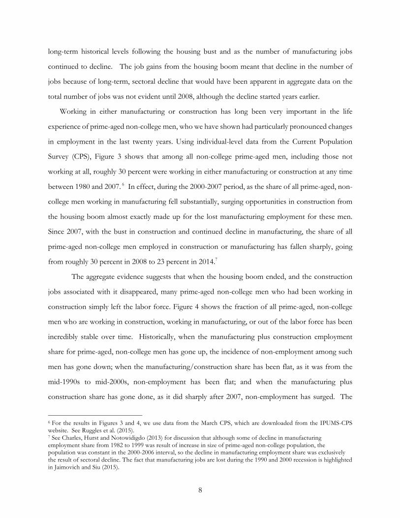
Working in either manufacturing or construction has long been very important in the life

experience of prime-aged non-college men, who we have shown had particularly pronounced changes

in employment in the last twenty years. Using individual-level data from the Current Population

Survey (CPS), Figure 3 shows that among all non-college prime-aged men, including those not

working at all, roughly 30 percent were working in either manufacturing or construction at any time

between 1980 and 2007. 6 In effect, during the 2000-2007 period, as the share of all prime-aged, non-

college men working in manufacturing fell substantially, surging opportunities in construction from

the housing boom almost exactly made up for the lost manufacturing employment for these men.

Since 2007, with the bust in construction and continued decline in manufacturing, the share of all

prime-aged non-college men employed in construction or manufacturing has fallen sharply, going

from roughly 30 percent in 2008 to 23 percent in 2014.7

The aggregate evidence suggests that when the housing boom ended, and the construction

jobs associated with it disappeared, many prime-aged non-college men who had been working in

construction simply left the labor force. Figure 4 shows the fraction of all prime-aged, non-college

men who are working in construction, working in manufacturing, or out of the labor force has been

incredibly stable over time. Historically, when the manufacturing plus construction employment

share for prime-aged, non-college men has gone up, the incidence of non-employment among such

men has gone down; when the manufacturing/construction share has been flat, as it was from the

mid-1990s to mid-2000s, non-employment has been flat; and when the manufacturing plus

construction share has gone done, as it did sharply after 2007, non-employment has surged. The

6 For the results in Figures 3 and 4, we use data from the March CPS, which are downloaded from the IPUMS-CPS website. See Ruggles et al. (2015). 7 See Charles, Hurst and Notowidigdo (2013) for discussion that although some of decline in manufacturing employment share from 1982 to 1999 was result of increase in size of prime-aged non-college population, the population was constant in the 2000-2006 interval, so the decline in manufacturing employment share was exclusively the result of sectoral decline. The fact that manufacturing jobs are lost during the 1990 and 2000 recession is highlighted in Jaimovich and Siu (2015).

9

negative association between the two series can be clearly seen in the top line in the figure, which

shows how remarkably constant the fraction of all prime-aged, non-college men engaged in these

three activities has been over time. It is this time series evidence which suggests that many of the

men not working in the construction and manufacturing sectors since 2007 have ceased being

employed altogether.

Masking: Local Labor Market Evidence An obvious concern about time-series evidence is that a temporal association between the

different series need not reflect a causal relationship. In particular, it could be that other unmeasured,

national-level shocks account for both the upward pattern in non-employment of prime-aged, non-

college males after 2007 and its sustained low level though 2015.

To investigate these concerns, we exploit variation across urban areas in the size of

manufacturing decline and the size of the local housing boom they experienced. We create a panel of

metropolitan statistical areas using data from the 2000 Census and from various years of the American

Community Survey individual-level and household-level extracts from the Integrated Public Use

Microsamples database (Ruggles et al., 2004). The analysis extends from 2000 (the first year during

the boom with reliable information in the Census at the level of metropolitan statistical areas) to 2012

(the midpoint of 2011-2013 American Community Survey data). These years span the 2000-2006

housing boom, the 2007-2009 housing bust, and several years after the end of the housing bubble

and the Great Recession. We compute employment rates and employment shares in various

occupations in each metropolitan statistical area.8 The primary analysis sample consists of non-

institutionalized, prime-aged men aged 25-54 without a four-year college degree.

Our measure of the decline in manufacturing in any given metropolitan statistical area, ,kMΔ

is the change in the fraction of the prime-aged, non-college male population in the Census/ACS

8 For the 2000 numbers, these means are from the 2000 Census. For the 2006 numbers, we pool the American Community Survey data from 2005 to 2007 to increase the precision of the metropolitan statistical area estimates. Similarly, we pool the 2011-2013 American Community Survey for the 2012 numbers.

10

employed in manufacturing industries over the relevant time period. In a simple model of housing

demand and supply, the effect of a shock that shifts housing demand will be a weighted sum of the

change in the price of housing and the change in housing supply, which can be proxied by the amount

of housing built. Our measure of the housing demand change, ,kHΔ is therefore the (log) change in

the average price of houses sold in the metropolitan statistical area plus the (log) change in the number

of building permits approved in the metropolitan statistical area MSA. We use house price data

from the Federal Housing Finance Agency (FHFA), mapping FHFA metro areas to the

Census/American Community Survey metro areas by hand. We use data on housing permits from

the Census Building Permits Survey, and match the metropolitan statistical area codes in the permits

data to the Census/ American Community Survey metro area codes by hand.9

Changes in both house prices and in the housing stock can affect employment. House prices

affect household wealth or liquidity and thus households' demand for goods and services produced

in the local market (Mian and Sufi 2011). Changes in the amount (or quality) of housing necessarily

involves construction activity such as demolition, renovation, home improvements, or new

construction. Our housing demand measure captures all of these effects.

Table 1 reports summary statistics for our sample of 275 metropolitan statistical areas with

non-missing labor market and housing market data. Our specific approach is to consider the effects

of two shocks to local markets during the years from 2000 to 2006: the change in the share of

population employed in manufacturing and our proxy for housing demand (based on changes in

housing prices and construction permits). We look at the effects of these changes on the employment

rate for non-college, prime-age men and the share of construction employment for this group in two

different time periods: the immediate effect of the shocks from 2000-2006 and the long-run effect

from 2000-2012. This set of variables will let us look at masking during the 2000-2006 period, and

the extent to which such effects might persist through 2012.

Panel A of Table 1 presents the means and standard deviation of the two local labor market

shocks we study. The top row shows that the average decline over the 2000-2006 period in the

9 See Charles, Hurst, and Notowidigdo (2015) for more details on the matching of the house price and housing permit data to the Census/ACS data.

11

manufacturing employment share across urban areas was -3.0 percentage points. The standard

deviation of 2.5 indicates that there was substantial variation across urban areas in this mean decline;

indeed, our analysis exploits this variation. The mean change in the housing demand proxy across

urban areas between 2000 and 2006 was 0.55 with a standard deviation of 0.57. Because the housing

proxy is the sum of the log changes in housing prices and building permits, this can be interpreted as

meaning that sum of housing prices and building permits rose by more than 50 percent across

metropolitan statistical areas, on average, with substantial variation across metro areas.

Panel B of Table 1 presents summary statistics for the change in the employment rate and in

the construction employment share for prime-aged non-college men for different periods between

2000 and 2012. These means are consistent with the aggregate patterns discussed before. Across

metropolitan statistical areas, the employment rate and overall construction share rose during the

2000-2006 boom, then fell sharply after 2007. By 2012, the share of non-college men working in

construction had returned to levels seen in 2000 in the average metro area, but their employment rate

remained substantially below 2000 levels, long after the end of the housing cycle.

We investigate the relationship between employment changes in a metropolitan statistical area

and manufacturing decline and housing demand shocks by estimating:

0 1 2 ,k k k k kE M XHβ β β η= + + + +Δ Δ Δ (1)

where ΔEk is either the change in employment in metropolitan statistical area or the change in the

construction share for one of the two time periods 2000-2006 or 2000-2012; the ,kMΔ and ,kHΔ

variables represent the local labor market shocks in manufacturing and housing; kX is a vector of

control variables and kη is a mean-zero regression error. The parameters 1β and 2β measure,

respectively, the effect of a change in local manufacturing employment and a change in local housing

demand on the change in employment. For simplicity, the results we present here are estimated with

these two coefficients in a single ordinary least squares regression model.10 The analysis is conducted

10 As we discuss in Charles et al. (2013), our results are similar in a more complicated two-equation model that allows for both direct effect of manufacturing decline on labor market outcomes as well as an indirect effect of manufacturing decline on labor market outcomes coming through the effect of manufacturing on housing demand. In the more complicated two-equation model, we can identify both the direct and indirect effect under the assumption that changes in local housing demand do not affect local manufacturing activity directly, which we show appears to be a reasonable assumption in our setting, since the housing boom has no significant effect on manufacturing employment. We also

12

in first differences and thus accounts for time-invariant differences across metropolitan statistical

areas. In each specification, the X vector follows Charles et al. (2015) and includes controls for the

share of employed workers with a college degree, the share of women in the labor force, and the

population of the metropolitan statistical area. All standard errors are clustered by state and are

weighted by the prime-age, non-college male population in 2000.

Table 2 presents the estimates of regression equation for the 2000-2006 and 2000-2012 time

periods. Each column reports the estimates from a separate equation. The point estimates in the first

column of the top panel imply that a one standard deviation decrease in manufacturing employment

given as 0.025 in Table 1 would, multiplied by the coefficient 0.471, decrease the employment rate

among non-prime-aged college men by about 1.2 percentage points during 2000-2006. Likewise, over

the same period, a one standard deviation increase in housing demand of 0.567 increased the

employment rate of prime-aged non-college men by about 1.3 percentage points during the 2000-

2006 period.

In column 2, we assess how the two local shocks affect the share of non-college men working

in construction in the metropolitan statistical area. We find no statistically significant relationship

between the manufacturing shock and construction employment. By contrast, construction

employment of non-college men increased the larger the housing demand shock in the metro area.

The portion of the employment increases experienced by non-college men as a result of the housing

boom that was attributable to the employment in the construction sector is the estimated effect of

the housing demand change in column 2 divided by the effect in column 1, or approximately 78

percent (that is, 0.018 divided by 0.023).

The regressions in the bottom panel of Table 2 examine how local manufacturing decline and

local housing market changes between 2000 and 2006 affect the longer-term change during the 2000-

2012 in outcomes for non-college men. The results indicate that the effect of manufacturing decline

show that the main results are similar using an instrumental variable for changes in housing demand that is formed by using sharp structural breaks in local housing prices that are interpreted as proxies for speculative activity. This instrument is described in detail in Charles et al. (2015). The similarity of the 2SLS estimates to the main OLS estimates reported in this paper is consistent with limited endogeneity bias during the 2000-2006 period, plausibly because this is a time period when a very large share of changes in housing demand is due to speculative activity rather than due to other changes in local labor demand.

13

during the 2000-2006 period on the long-term employment of non-college men was, in fact, quite

durable. Indeed, the effects of the manufacturing decline on employment growth between 2000 and

2012 were fairly similar to the effects shown for the 2000-2006 change. The results for the

employment effects of housing demand changes, however, differed sharply over 2000-2006 and the

longer 2000-2012 period. In particular, we find that changes in estimated housing demand during the

2000-2006 housing boom period had no significant long-term effect on employment of non-college

men over the 2000-2012 period, either for the overall employment rate or for the share of

employment in construction.

This evidence across metro areas suggests that the 2000-2006 housing boom had a masking

effect on the loss of manufacturing jobs during those years, but this masking was undone during the

housing bust. The negative employment effects of the housing bust were similar in magnitude to the

positive employment effects of the preceding housing boom. Over the entire period from 2000 to

2012, the strong relationship between the local decline in manufacturing the employment rate of non-

college men in a metropolitan statistical area was not affected by changes in housing demand in the

metro area during the 2000-2006 boom period.

Individual-Level Masking: Evidence from Displaced Manufacturing Workers

Our local labor markets analysis suggests that masking occurred both within and between

metropolitan areas. 11 What is not clear is the extent to which this masking within metro areas was

because different types of workers were affected by manufacturing and housing market shocks, and

how much, if any, was because some of the specific workers who lost jobs in manufacturing found

employment in housing during the boom, only to lose them when housing collapsed.

11 In Charles et al. (2013), we present results from more in-depth analysis to assess how much of masking is between-city and within-city. We find evidence of both types of masking; many cities either experienced a large housing boom or manufacturing decline between 2000-2006 but not both. Within cities, we find manufacturing affected older adults relatively more than younger adults, while our estimates suggest that the housing boom affected employment rates of older and younger adults similarly.

14

To determine the extent to which the specific workers displaced from manufacturing because

of the decline in that sector were re-employed in housing-related sectors, we use individual-level data

from the Displaced Worker Survey, which is conducted every two years as part of the Current

Population Survey.12 This survey focuses on individuals who have been displaced from a job at some

point during the preceding three years. In addition to the standard battery of questions about current

employment and demographics, respondents are asked detailed questions about their previous job.

We construct a sample consisting of all men aged 25-54 without a college degree in the 1994-2006

waves of the Displaced Worker Survey who were displaced from jobs in the manufacturing sector.

Displacements in this sample occurred between 1992 and 2005.

The resulting sample of 2,161 persons is relatively small, but it contains geographic identifiers

that allow us to sort displaced workers by the size of the housing boom that their local metropolitan

statistical area experienced. We create an indicator variable to denote displacement between 1997

and 2005, years in the midst of the national housing boom. Persons for whom this indicator was zero

were therefore displaced between 1991 and 1996 (in the years before the housing boom). For each

displaced worker in our sample, we also know whether they lived in “housing boom metropolitan

statistical area,” which we define to be those whose especially large housing booms placed them in

the top one-third in the distribution of the housing demand change measure, ΔHk.13 Intuitively, this

captures the metro areas that had especially large increases in housing demand. We estimate a model

of the form:

1 kHousingBoom MSA Boom Perio1{ d} 1{ }ikt k t ikt ikty eXβ α δ + Γ +++= × (2)

where y is either (in different specifications) re-employment or re-employment in construction of a

displaced worker i in market k at time t . The terms kα and tδ are MSA and time period fixed

12 See Farber (2015) for more information on DWS data and a detailed investigation of labor market outcomes of workers displaced during the Great Recession (compared to earlier recessions). 13 The evidence is fairly similar using other thresholds such as like the top quartile or top 10 percent. It is also is robust to residualizing housing demand change to manufacturing decline proxy and other controls, so that the definition of a housing boom metro area is based on change in housing demand that is above and beyond what one would predict from manufacturing decline and other variables. See Charles, Hurst, Notowidigdo (2013) for more details.

15

effects, respectively, and the vector X contains individual level controls like years of education, union

status in the last job, and a fifth-order polynomial in age.

The coefficient 1β from this regression is a difference-in-difference estimate of the effect of

being in a metropolitan statistical area with a large housing boom on the probability of becoming re-

employed for a worker displaced from manufacturing during the years of the housing boom. We

study two outcomes: whether the person reported employment as of the survey year, and whether

the person was employed in construction as of the survey year.

Table 3 presents the estimated effects, with associated standard errors clustered by state. For

each outcome in Table 3, we present two difference-in-difference specifications. The first

specification (in columns 1 and 3) includes fixed effects for metropolitan statistical areas and adds

fixed effects for each year of displacement. The second specification (columns 2 and 4) adds the

individual-level controls to the specifications in columns 1 and 3. The results for employment suggest

a substantial amount of “individual-level masking.” We find that manufacturing workers displaced in

markets with especially large housing demand increases during the 2000-2006 period were around 9

percentage points less likely to be re-employed. This result holds across various specifications, and

is large relative to the mean of the outcome variable of 69 percent. These estimates imply that,

compared to displaced workers in other markets, individuals displaced from manufacturing in a

metropolitan statistical area with a large housing boom were roughly 13 percent more likely to be re-

employed relatively quickly after being displaced.

The results for construction re-employment are also striking. In the results in columns 3 and

4, the point estimates suggest that displaced manufacturing workers were much more likely to be

employed in construction if they became displaced in markets with big housing demand increases.

The point estimate of 0.049 suggests displaced manufacturing workers in markets during the years of

the housing boom in markets with big booms were likely to find re-employment in construction at a

rate that was roughly 50 percent of the overall employment effect. These results suggest that a

meaningful share of the employment “masking” for non-college men at the individual level came

through construction employment.

16

Collectively, these results provide evidence of individual-level masking. Had there been no

temporary housing boom from the late 1990s through the mid-2000s, many workers displaced from

manufacturing because of the ongoing decline in that sector would have been significantly more likely

to end up in non-employment during this time period.

Conclusion

This paper argues that employment gains from the recent national housing boom “masked”

the adverse employment effects of declining manufacturing in the years before the Great Recession.

What has been called the national “employment sag” that began in 2000 would therefore have been

even larger in the absence of this masking in the years before the Great Recession. We show that

aggregate masking occurred overall in the national time series, both between and within cities, and at

the individual level. The sharp decline in employment that occurred during the Great Recession was

due not only to cyclical forces, but also to the fact that the massive housing bust, which coincided

with the start of the recession, “unmasked” the adverse employment effects of more than a decade

of systematic manufacturing decline. Persistently low employment in the several years after the end

of the recession point to ongoing importance of these structural factors.

Our analysis focuses on non-college men in the United States, but the mechanism we have

highlighted is more broadly relevant. For example, many prime-aged non-college women also lost

jobs from declining manufacturing. When we do an analysis across metropolitan areas similar to that

presented for their male counterparts, we find that the local decline in manufacturing had an effect

on the employment rate of non-college women that is nearly two-thirds the size of the effect for non-

college men. While housing booms in local labor markets increased employment for non-college

women, as well, for them virtually all of the increased employment came in services and related sectors

(such as finance, insurance and real estate) rather than in construction. Outside the U.S., Hoffman

and Lemieux (2014) have emphasized the perhaps surprising explanatory power of construction

17

employment in accounting for cross-country patterns in employment growth in the aftermath of the

Great Recession. We therefore speculate that housing booms may have “masked” the adverse effects

of manufacturing decline in other countries, as well.

Our results shed light on the question of how much of the recent decline in employment rates

are the result of cyclical factors, and how much from structural factors like the long-term decline in

manufacturing and associated losses in routine jobs. The answer to this question is crucially important

because of its implications for policy response to the falling employment. Traditional monetary and

fiscal policy tools, such as temporary interest rate cuts, tax rebates or increases in government

spending, are designed to provide a temporary boost to labor demand. These tools can thus offset

temporary declines in hiring arising from cyclical factors like short-lived tightening of credit markets

or transitory increases in uncertainty, temporarily boosting employment until the economy returns to

its normal level. By contrast, there is little reason to suppose that these traditional monetary and fiscal

tools can satisfactorily address employment decline arising from structural factors.

What policies might be effective in the future at raising employment rates, particularly among the

relatively less-skilled? One set of options might be policies that encourage skill investment among

the non-college educated, thereby directly addressing their skill deficits and hopefully raising their

long-term employment prospects. It has historically proved difficult to get people to alter their

human capital choice using traditional policies like targeted taxes or educational subsidies. It is

therefore likely that in order to encourage workers who have traditionally worked in routine

occupations to obtain the skills demanded in the current economic environment, there will have to

be experimentation with new policies ideas to spur schooling investment.

Some have suggested that the portion of employment decline attributable to structural factors

might be addressed by the undertaking of large-scale, publicly-financed infrastructure projects

(Summers (2014)). A potential benefit of the public undertaking of such projects would be the boost

to employment opportunities they would provide for less-educated workers, particularly if the

projects raised the overall demand for such workers rather than simply re-allocated them from the

private to public sectors. Such investments could yield longer term gains for lower skilled workers

if these investments in infrastructure led to broader productivity gains within the economy.

18

But, publicly financed infrastructure investments are not without important costs. One set of

these are the various efficiency costs associated with raising public funds, even in this period of

historically low interest rates. Another potential cost is that the necessarily temporary nature of

infrastructure projects might have the unintended effect of adversely affecting skill-upgrading among

non-college persons. Unless infrastructure construction translates into permanent increases in labor

demand for lower skilled workers, the temporary gain in employment such projects would provide

would be similar to the gain in employment from the hot housing market in the early 2000s, in the

sense that underlying weakness in the labor market would be masked for a time before being revealed

when the projects ended.

In other work we have found evidence suggesting that the abundant but temporary employment

opportunities provided by the housing boom during the 2000s caused some young non-college

persons to delay college-going, presumably because they erroneously believed that housing-related

job opportunities would exist in the longer-term (Charles, Hurst, and Notowidigdo 2015). Many of

these individuals did not return to college when those labor market opportunities vanished during the

housing bust, thereby delaying the chance to obtain skills demanded in sectors like high-tech

manufacturing and tradeable services. There is thus a persistently lower level of college attendance

among the specific birth-year cohorts who were of college-going age during the housing boom period.

Employment masking from temporary public construction projects in the future could have a similar

effect.

The structural interpretation of the declining employment to population ratio highlights another

layer to rising inequality in the United States in income and consumption between more skilled and

less skilled workers during the last three decades. Our work highlights changes in employment

inequality between higher and lower skilled workers since the early 2000s. While this fact has been

highlighted by others (Aguiar and Hurst, 2009 and Attanasio, Hurst and Pistaferri, 2014), our work

shows that the decline in manufacturing employment has contributed to the increased inequality in

employment propensities. To the extent that employment propensities translate to earnings, our

results account for some portion of the increased earnings inequality between higher and lower skilled

workers that has occurred since the early 2000s.

19

Our paper is silent on the welfare implications of the masking phenomenon that we document.

As noted above, in companion work, we have documented how the housing boom altered skill

acquisition for lower skilled men and women during the early 2000 boom years. However, there may

have been benefits of the masking phenomenon. For example, we show evidence that masking from

the housing boom postponed and thereby soften the economic costs of structural transition. The fact

that the boom appears to have ameliorated the employment losses that would have otherwise

occurred because of manufacturing decline may have given regions time to engage in difficult

reallocation of workers across sectors, thereby easing some of the costs of adjustment. Time to

develop new tradeable industries that would likely to be competitive in the future given the changing

landscape of import competition may have been one benefit of masking. How this benefit compares

to the costs of altering human capital decisions has not been studied. In future work, it would be

useful to quantify the importance of these different factors in terms of individual welfare.

We close with the observation that the phenomenon of employment masking studied in this paper

may be important for understanding the economic consequences of sectoral shifts more broadly. A

growing literature finds that large structural shifts such as the shift from agriculture to manufacturing

work, and from routine jobs to non-routine jobs, have important macroeconomic effects and may

significantly affect economic growth. In some cases, these structural shifts proceeded with what

appears to have been minimal effects on aggregate employment. Results from our work and that of

others suggest, by contrast, that the decline of manufacturing may be associated with significant

adverse effect on aggregate employment. Whether adverse macroeconomic effects arise from a

structural shift may depend on the ability of workers to shift between sectors and occupations, either

immediately or perhaps with some modest delay after re-training or some other form of human capital

accumulation. Understanding the process of how workers switch sectors in response to large

structural shifts is an important area for future research.

 

20

Acknowledgements

This paper contains some results that appeared in a previously distributed NBER working paper entitled “Manufacturing Decline, Housing Booms, and Non-employment” (NBER Working Paper No. 18949). We thank John Bound, Tom Davidoff, Matt Gentzkow, Ed Glaeser, and Erzo Luttmer for their detailed feedback, and we thank Hank Farber and Tom Lemieux for their comments as discussants.

 

   

   

21

REFERENCES Aaronson, Daniel, Luojia Hu, Arian Seifoddini, Daniel G. Sullivan (2015). “Changing Labor Force Composition and the Natural Rate of Unemployment,” Federal Reserve Bank of Chicago Working Paper #338. Acemoglu, Daron, David Autor, David Dorn, Gordon H. Hanson, and Brendan Price (2016), “Import Competition and the Great U.S. Employment Sag of the 2000s,” Journal of Labor Economics, forthcoming. Aguiar, Mark and Erik Hurst (2009). The Increase in Leisure Inequality: 1965-2005. Washington, D.C., American Enterprise Institute. Attanasio, Orazio, Erik Hurst and Luigi Pistaferri (2015). “The Evolution of Income, Consumption and Leisure Inequality in the United States, 1980-2010,” in Improving the Measurement of Consumer Expenditures, eds Christopher Carroll, Thomas Crossley, and John Sabelhaus, National Bureau of Economic Research. Autor, David H., and David Dorn (2013). "The Growth of Low-Skill Service Jobs and the Polarization of the US Labor Market." American Economic Review, 103(5): 1553-97. Autor, David, David Dorn, and Gordon Hanson (2013). "The China Syndrome: Local Labor Market Effects of Import Competition in the United States," American Economic Review. Autor, David and Mark Duggan (2006). “The Growth in the Social Security Disability Rolls: A Fiscal Crisis Unfolding,” Journal of Economic Perspectives, 20(3), 71 - 96. Autor, David and Mark Duggan (2003). “The Rise in the Disability Rolls and the Decline in Unemployment,” Quarterly Journal of Economics, 118(1), 157 - 206. Autor, David, Frank Levy, and Richard Murnane (2003). "The Skill Content Of Recent Technological Change: An Empirical Exploration," The Quarterly Journal of Economics, 118(4): 1279-1333. Autor, David, Nicole Maestas, Kathleen Mullen, and Alexander Strand (2015). “Does Delay Cause Decay? The Effect of Administrative Decision Time on the Labor Force Participation and Earnings of Disability Applicants”, NBER Working Paper 20840. Baker, Scott, Nick Bloom, and Steve Davis (2013). "Measuring Economic Policy Uncertainty", Stanford University Working Paper. Berman, Eli, John Bound, and Zvi Griliches (1994), “Changes in the Demand for Skilled Labor within U.S. Manufacturing: Evidence from the Annual Survey of Manufacturers,” Quarterly Journal of Economics 109(2): 367-397. Blanchard, Olivier and Lawrence F. Katz (1992). "Regional Evolutions," Brookings Papers on Economic Activity, 23(1): 1-76.

22

Bound, John and Harry J. Holzer (1993). "Industrial Shifts, Skills Levels, and the Labor Market for White and Black Males," The Review of Economics and Statistics, 75(3): 387-96. Charles, Kerwin, Erik Hurst, and Matthew J. Notowidigdo (2013). “Manufacturing Decline, Housing Booms, and Non-Employment,” NBER Working Paper #18949. Charles, Kerwin, Erik Hurst, and Matthew J. Notowidigdo (2015). “Housing Booms and Busts, Labor Market Opportunities, and College Attendance,” NBER Working Paper #21587. Chodorow-Reich, Gabriel. 2014. “The Employment Effects of Credit Market Disruptions: Firm-level Evidence from the 2008-09 Financial Crisis,” Quarterly Journal of Economics, 129 (1): 1-59. Davis, Steven J. and John Haltiwanger (2014). “Labor Market Fluidity and Economic Performance,” NBER Working Paper No. 20479. Eggertsson, Gauti B. and Paul Krugman (2012). “Debt, Deleveraging, and the Liquidity Trap: A Fisher-Minsky-Koo Approach,” The Quarterly Journal of Economics, 127 (3): 1469-1513. Farber, Henry S. (2015). “Job Loss in the Great Recession and its Aftermath: U.S. Evidence from the Displaced Worker Survey,” Working Paper 589, Industrial Relations Section, Princeton University. Farber, Henry S. and Robert G. Valetta (2013). “Do Extended Benefits Lengthen Unemployment Spells? Evidence from Recent Cycles in the U.S. Labor Market,” Working Paper. Fernandez-Villaverde, Jesus, Pablo Guerron-Quintana, Keith Kuester, and Juan Rubio-Ramirez (2013). “Fiscal Volatility Shocks and Economic Activity,” Working Paper. Giroud, Xavier and Holger Mueller (2015). “Firm Leverage and Unemployment during the Great Recession,” Working Paper. Greenstone, Michael, Alex Mas, and Hoai-Luu Nguyen (2015). “Do Credit Market Shocks Affect the Real Economy? Quasi-Experimental Evidence from the Great Recession and 'Normal' Economic Times,” Working Paper. Guerreri, Veronica and Guido Lorenzoni (2015), “Credit Crises, Precautionary Savings and the Liquidity Trap,” Working Paper. Hagedorn, Marcus, Fatih Karahan, Iourii Manovski, and Kurt Mitman (2015). “Unemployment Benefits and Unemployment in the Great Recession: The Role of Macro Effects,” Working Paper. Hall, Robert (2011). “The Long Slump”, American Economic Review, 101(2), April, pp. 431-469. Hall, Robert (2014). “Secular Stagnation”, Working Paper. Hoffman, Florian and Thomas Lemieux (2014). “Unemployment in the Great Recession: A Comparison of Germany, Canada and the United States,” NBER Working Paper #20694.

23

Jaimovich, Nir and Henry Siu (2015). “The Trend is the Cycle: Job Polarization and Jobless Recoveries,” Working Paper. Johnston, Andrew and Alex Mas (2015). “Potential Unemployment Insurance Duration and Labor Supply: The Individual and Market-Level Response to a Benefit Cut”, Working Paper. Kroft, Kory, Fabian Lange, Lawrence Katz, and Matthew Notowidigdo (2016). “Long-Term Unemployment and the Great Recession: The Role of Composition, Duration Dependence, and Non-Participation”, Journal of Labor Economics, forthcoming. Maestas, Nicole, Kathleen J. Mullen and Alexander Strand (2013). “Does Disability Insurance Receipt Discourage Work? Using Examiner Assignment to Estimate Causal Effects of SSDI Receipt.” American Economic Review, 103(5), 1797-1829. Maestas, Nicole, Kathleen J. Mullen, and Alexander Strand (2015). “Disability Insurance and the Great Recession,” RAND Working Paper WR-1088. Mian, A. and Sufi, A. (2014). “What Explains the 2007–2009 Drop in Employment?” Econometrica, 82: 2197–2223. Mian, Atif and Amir Sufi (2011). "House Prices, Home Equity-Based Borrowing, and the U.S. Household Leverage Crises", American Economic Review, 101, 2132-56. Moffit, Robert (2012). "The U.S. Employment-Population Reversal in the 2000s: Facts and Explanations", Brookings Papers for Economic Activity, Fall, 201-264. Mondragon, John. (2015). “Household Credit and Employment in the Great Recession,” Working Paper. Mulligan, Casey (2012). The Redistribution Recession: How Labor Market Distortions Contracted the Economy. Oxford University Press, New York. Pierce, Justin R. and Peter K. Schott (2016), “The Surprisingly Swift Decline of U.S. Manufacturing Employment,” American Economic Review, forthcoming. Rothstein, Jesse (2012). “Unemployment Insurance and Job Search in the Great Recession", Brookings Papers on Economic Activity, Spring, 143-196. Ruggles, Steven, Matthew Sobek, Trent Alexander, Catherine Fitch, Ronald Goeken, Patricia Kelly Hall, Miriam King, and Chad Ronnander (2015). Integrated Public Use Microdata Series. Minneapolis, MN: Minnesota Population Center. Sahin, Aysegul, Joseph Song, Giorgio Topa, and Giovanni Violante (2014). "Mismatch Unemployment", American Economic Review.  Sloane, Carolyn (2015). “Where are the Workers? Technological Change, Rising Disability and the Employment Puzzle of the 2000s: A Regional Approach”. University of Chicago Working Paper  

24

Summers, Lawrence. (2014) “U.S. Economic Prospects: Secular Stagnation, Hysteresis, and the Zero Lower Bound” http://larrysummers.com/wp-content/uploads/2014/06/NABE-speech-Lawrence-H.-Summers1.pdf

Share of Population Employed in Manufacturing, ΔMk 275 -0.030 0.025Housing Demand, ΔHk_ 275 0.552 0.567

Employment Rate for Non-College Men 275 0.019 0.040Construction Employment Share for Non-College Men 275 0.027 0.019

Employment Rate for Non-College Men 275 -0.003 0.028Construction Employment Share for Non-College Men 275 0.008 0.011

Panel A: Manufacturing Decline and Changes in Housing Demand

Panel B: Changes in Total Employment and Construction Employment

2000-2006 Changes

2000-2006 Changes

2000-2012 Changes

Notes: This table reports the summary statistics for the baseline sample of 275 metropolitan areas (MSAs)across the time periods studied in the regressions that use the Census/ACS data. The Change in HousingDemandvariable is constructed by adding the change inhousing prices (from FHFA house priceindex) to thechange in housing permits (from Census Building Permits Survey). This procedure creates a proxy for thechange in housing demand in an MSA between 2000 and 2006; see Charles, Hurst, Notowidigdo (2015) formore details. Allof the reported sample statistics are computed using the 2000 populationof prime-aged, non-college men in the MSA (from Census/ACS) as weights, since these weights are used in all of the regressions.

Table 1Descriptive Statistics of Manufacturing Decline and Housing Booms Across Cities

N MeanStd. Dev.

25

Dependent Variable: Employment Rate

Construction Employment

Share (1) (2)

0.471 0.009(0.090) (0.063)

0.023 0.018(0.006) (0.004)

R2 0.76 0.45

0.377 -0.031(0.085) (0.043)

0.007 0.005(0.007) (0.002)

R2 0.61 0.35

N 275 275Include baseline controls y y

Panel B: Change Between 2000 and 2012Change in Share of PopulationEmployed in Manufacturing, ΔMk

[Manufacturing Decline]

Change in Housing Demand, ΔHk

[Housing Shock]

Notes: This table reports results of estimating equation (1) by OLS for various samples. A 0.01 unit decrease in the Manufacturing Decline measure corresponds to a 1 percentage point decline in share of prime-age (25-54) non-college-educated male population employed in manufacturing. A 1 unit change in housing demand measure corresponds to 1 log point increase in housing demand proxy described in Table 1.The baseline controls include the initial (year 2000) values of the share of employed workers with a college degree, the share of women in the labor force, and the log population in the MSA. Standard errors, adjusted to allow for an arbitrary variance-covariance matrix for each state, are in parentheses.

Table 2Manufacturing Decline, Housing Booms, and Cross-City Masking

Panel A: Change Between 2000 and 2006Change in Share of PopulationEmployed in Manufacturing, ΔMk

[Manufacturing Decline]

Change in Housing Demand, ΔHk

[Housing Shock]

Sample: Prime-Age, Non-College Men

26

Dependent Variable:

(1) (2) (3) (4)

Difference-in-difference estimate of effect of housing boom:Displaced between 1997 and 2005 × 0.095 0.092 0.049 0.047 Housing Boom MSA (0.044) (0.043) (0.019) (0.019)

Mean of dependent variable 0.693 0.693 0.056 0.056N 2161 2161 2161 2161

R2 0.145 0.152 0.119 0.125

Include MSA fixed effects y y y yInclude Displacement Year fixed effects y y y yInclude Individual-level controls y y

Notes: This table reports OLS estimates of equation (2). The first row reports the Difference-in-Difference estimate of the effect of being displaced during housing boom time period within an MSA that was experiencing a housing boom. An MSA is defined to be a "Housing Boom MSA" if it has value in the top third of the distribution of 2000-2006 changes in housing demand as defined in Table 1. If a displaced worker is not in one of the MSAs with housing market data or is in a non-metro region, then this indicator is set to 0. The additional individual-level controls in columns (2) and (4) are the following: education, union status in last job, and 5th-degree polynomial in age. Standard errors are clustered by state and are in parentheses.

Table 3Displaced Manufacturing Workers, Housing Booms, and Individual-Level Masking

Employed in ConstructionEmployed

Sample: Non-College Men, Age 25-54, Manufacturing Workers Displaced 1992-2005Source: CPS Displaced Worker Surveys, 1994-2006

27

Figure 1

Notes: This figure uses data from 1980-2015 March CPS. The “Higher Skilled” Men and Women are all prime-age adults (aged 25-54) who have at least a four-year college degree. Adults with lower levels of education are “Lower Skilled.” The figures calculate employment rates as share of total population of each group using individual-level survey weights.

0.50

0.55

0.60

0.65

0.70

0.75

0.80

0.85

0.90

0.95

1.00

1980

1981

1982

1983

1984

1985

1986

1987

1988

1989

1990

1991

1992

1993

1994

1995

1996

1997

1998

1999

2000

2001

2002

2003

2004

2005

2006

2007

2008

2009

2010

2011

2012

2013

2014

2015

Employment Rate, Prime-Age Individuals1980-2015 Current Population Survey

Lower Skilled Men

Lower Skilled Women

Higher Skilled Men

Higher Skilled Women

28

Figure 2

Notes: This figure uses aggregate data from the Bureau of Labor Statistics on monthly employment in manufacturing and construction sectors.

0

2,000

4,000

6,000

8,000

10,000

12,000

14,000

16,000

18,000

20,000

22,000

24,000

26,000

1980

1981

1982

1983

1984

1985

1986

1987

1988

1989

1990

1991

1992

1993

1994

1995

1996

1997

1998

1999

2000

2001

2002

2003

2004

2005

2006

2007

2008

2009

2010

2011

2012

2013

2014

2015

Total Monthly U.S. Manufacturing Employment (in 1,000s)1980M1-2015M9

Manufacturing Employment

Construction Employment

Manufacturing + Construction

29

Figure 3

Notes: This figure uses data from 1980-2015 March CPS, restricted to prime-age men with education below a four-year college degree. The figures calculate employment shares as a share of total population using individual-level survey weights.

0.00

0.05

0.10

0.15

0.20

0.25

0.30

0.35

0.40

1980

1981

1982

1983

1984

1985

1986

1987

1988

1989

1990

1991

1992

1993

1994

1995

1996

1997

1998

1999

2000

2001

2002

2003

2004

2005

2006

2007

2008

2009

2010

2011

2012

2013

2014

2015

Construction and Manufacturing Employment Shares Non-College Men Aged 25-54, 1980-2015

Share Manufacturing or Construction

Share Construction

Share Manufacturing

30

Figure 4

Notes: This figure uses data from 1980-2015 March CPS, restricted to prime-age men with education below a four-year college degree. The figures calculate non-employment rates and employment shares as a share of total population using individual-level survey weights.

0.10

0.20

0.30

0.40

0.50

0.60

1980

1981

1982

1983

1984

1985

1986

1987

1988

1989

1990

1991

1992

1993

1994

1995

1996

1997

1998

1999

2000

2001

2002

2003

2004

2005

2006

2007

2008

2009

2010

2011

2012

2013

2014

2015

Construction, Manufacturing, and Non-Employment Shares Non-College Men Aged 25-54, 1980-2015

Manufacturing, Construction and Non-Employment Share

Non-Employment Share

Manufacutring and Construction Share

31