FORTHCOMING IN HISTORY OF ECONOMIC IDEAS

The Making of the Leif Johansen Multi-Sectoral Model

By

Olav Bjerkholt Department of Economics, University of Oslo & Statistics Norway

P.O. Box 1095 Blindern 0317 Oslo, NORWAYdf tel +47 22855138, fax +47 22855035 olav.bjerkholt@econ.uio.no

Abstract

The paper traces the roots of Leif Johansen’s 1960 monograph A Multi-Sectoral Study of

Economic Growth, recognized as the first computable general equilibrium (CGE) model.

Although Johansen might have been much attracted towards a purely theoretical study of a

multi-sectoral equilibrium growth process he chose to construct an empirical model,

calibrated to fit the Norwegian economy in 1950. Johansen’s model combined Leontief’s

input-output analysis with Solow-type production functions and a Frisch-influenced

specification of consumption demand. His work became influential on the further CGE

development. Johansen died at the age of 52 in 1982 and is regarded as the (only) intellectual

heir of his teachers Ragnar Frisch and Trygve Haavelmo in originality and profoundness.

Keywords: Multi-sectoral, General equilibrium, CGE/AGE, Leif Johansen

JEL classification: B31, D58, C68, O41

2

1. Introduction*

Leif Johansen was an exceptionally gifted Norwegian economist who died in 1982 at the age

of 52. His doctoral dissertation, published as A Multi-Sectoral Study of Economic Growth was

an empirical model, recognized as having been the first computable general equilibrium (CGE)

model.1 The aim of the paper is to trace the roots of the Johansen’s pioneering contribution

and the path he followed towards its completion in 1959.

Leif Johansen completed secondary school in Oslo in 1948. His father was an army

lieutenant and member of the communist party. Other top-ranked students with a gift for

mathematics would more typically at the time choose to study at the polytechnic in

Trondheim. Johansen’s choice may have been related to his political and social interests, he

was a member of the communist youth league and well read in Marxist literature.

The Institute of Economics at the University of Oslo was run by Ragnar Frisch. In the

early post-war period the demand for economists outran supply, the inflow to the economics

study swelled, cf. BJERKHOLT (2005a). Trygve Haavelmo, who had worked with Frisch from

1933 until he went to the USA in 1939, cf. BJERKHOLT (2005b), returned to Norway after the

war and was appointed professor at the university in the spring of 1948. Leif Johansen had

Frisch and Haavelmo as teachers in economics and statistics until he graduated in 1954.2

Johansen’s exceptional talent was recognized while he was still an undergraduate.

* I am most grateful for highly constructive comments from two anonymous referees. I have benefited from comments on earlier versions from participants at the conference General Equilibrium as Knowledge. From Walras Onwards, Paris, 6-8 September 2007, from seminars in University of Copenhagen and the Norwegian University of Science and Technology, and from Peter Dixon, Tore Johansen, Benjamin Mitra-Kahn, Jørn Rattsø, Sherman Robinson, Tore Thonstad, and not least from Bjørn Thalberg’s memorial paper on Leif Johansen, THALBERG, 2000. I am entirely responsible for remaining errors and shortcomings. 1 JOHANSEN 1960a. According to KEHOE et al. 2005 numerical applications of general equilibrium started with the work of JOHANSEN (1960a) and HARBERGER 1962. The latter was a model with only two production sectors for calculation of the incidence of the U.S. corporate income tax. CGE models are also known as applied general equilibrium (AGE) models, although these acronyms were used by different traditions within this genre. In Australia CGE models were in recognition of the Johansen’s pioneering work denoted “Johansen-style model” and “Johansen class of multisectoral models”, DIXON ET AL. 1982, 1. 2 In the preface to his dissertation Johansen acknowledged his indebtedness to Frisch and Trygve Haavelmo but did not give any details, as that would be “evident to anyone who is familiar with that background.” JOHANSEN 1960a, Preface.

3

Johansen embarked in 1956 upon a research project on the relation between industries

in a well developed economy under economic growth. Johansen was well prepared for such a

task after his studies and assistant work with Frisch and Haavelmo, and from his own research

and studies of the international literature. The academic year 1958/59 Johansen spent in

Cambridge at Richard Stone’s Department of Applied Economics, during that year he also

visited Jan Tinbergen in Rotterdam.3

The project resulted in a book, submitted as a doctoral dissertation at the University of

Oslo and defended in 1961. The first review of Johansen’s book gave it unique praise as “a

model that comes closer to the Walrasian equations of general equilibrium than any that has

been previously used in empirical studies” (CHENERY, 1961, 121).

Section 2 sketches briefly some of Ragnar Frisch’s main research ideas and activities

in the early post-war years, while section 3 surveys experience gained by Leif Johansen as a

student and young graduate at the Institute. Section 4 recapitulates Johansen’s own survey of

the multi-sectoral growth. Section 5 summarizes the analytic core of Johansen’s model and

choices he made in the model specification. Section 6 conveys some of Frisch’s reactions to

on Johansen’s dissertation, and section 7 concludes.

2. Frisch’s Institute of Economics in the early post-war years

Ragnar Frisch and other early econometricians strived in the 1930s towards more rigour in

theoretical analysis and suitable statistical methods in data analysis. Frisch’s contribution to

business cycle analysis (BJERKHOLT 2007) received great attention and together with

Tinbergen’s modelling attempts it is regarded by Arrow (2005) as the “first applied general

(i.e. complete) models in the literature” and by implication as steps towards general

3 Johansen traveled with a Rockefeller fellowship, which was more typical used for visiting American universities. That was not an option for Leif Johansen, who was a card carrying communist, and took it for granted that a visa application would be rejected, cf. BORCH 1987. Leif Johansen kept a diary during his study year abroad, leaving us with some clues of his experiences gained, cf. THALBERG 2000, 102-112.

4

equilibrium modelling, although they were more in the tradition that developed into

macroeconomics.

After the liberation of Norway in May 1945 an all-party accord lay down guidelines

for economic policy in the reconstruction period. The Labour Party came to power after

elections in the autumn of 1945 with a broad concept of national economic management. The

planning system which grew up to administer the post-war economy had few ideological

overtones, it aimed at comprehensive coordination of all government agencies and strict

rationing and regulation measures for consumers and enterprises, within the conceptual

framework of ‘national budgeting’.4

On this overall background a key priority for Frisch’s Institute of Economics was to

educate a sufficient number of economists up to these tasks and, furthermore, provide tools

needed for managing the economy. Frisch (1946) marked the change of times, conveying that

the time had come for applying econometrics. He predicted a vast increase in the demand for

economists in government: “one feels the need of men who understand how the big economic

issues, employment, investment, labour, living costs, fiscal policies, etc. gear into each

other…essentially a quantitative problem…to general macroeconomics.” He also suggested

how this demand could be met. The remedy is “large organizations where young economists

can be trained in free research work in general economics and … econometrics.”5 Hardly

anyone could fit this recruiting description better than young Leif Johansen who matriculated

at the University of Oslo as a student of economics in September 1948.

Frisch coined at that time his key term decision model and embarked on a

comprehensive program of modelling. His former students had got into powerful positions,

some even reached the commanding heights of economic policy. Frisch built a disequilibrium

4 Yet another term coined by Frisch who also had pioneered national accounting in Norway. 5 Quoted from FRISCH 1946, 1-4. Frisch added somewhat ominously that econometrics was a powerful tool and dangerous when abused: “it should only be put into the hands of really first-rate men. Others should be absolutely discouraged from taking up econometrics” (FRISCH 1946, 4).

5

model for constrained post-war rationing situation (FRISCH 1955) and developed techniques

for interaction between model use and policy analysis, later known as target-instrument

analysis.6 He also let groups of students representing different political parties play with

model, vying with each other in achieving the best result.

Frisch embraced the input-output analysis of Wassily Leontief in the early 1950s and

applied it in a series of models. His modelling philosophy comprised a classification of stages

in modelling, from the low of on-looker models to the ultimate stage of the optimalization

approach, i.e. a model comprising a preference function and a mathematical programming

technique for locating the most preferred solution among feasible alternatives, FRISCH 1962,

254.

Another conceptual distinction in Frisch’s modelling philosophy of some importance

for Frisch’s view on Johansen (1960a) was that of selection versus implementation:

“In the selection analysis we are able to build the theory on a precise and quantitatively

formulated model with a fair degree of correspondence with realities. … In the implementation

problem we have to consider any effects and behaviouristic relations that it is – at least so far –

difficult to measure with a satisfactory degree of precision…After the selection problem is

solved, one will take up the implementation problem.” FRISCH 1963, 22.

Frisch took upon himself the two main challenges in the optimalization approach: the

formalization and estimation of preferences and the mathematical programming techniques

required for solving such models.7

One has to admire the ambition in Frisch's endeavour, albeit he was naïve in his

understanding of the political system. Could the execution of economic policy really be put in

the hands of experts who would base their decisions on the estimated preferences of political

6 Target-instrument analysis is often and perhaps fairly credited to Tinbergen but note the remark: “The core of the theory in this book is nothing but an application of the notion of ‘decision models’ as introduced by Ragnar Frisch”, TINBERGEN 1966, Preface. 7 This and preceding paragraphs draws on BJERKHOLT 1998, cf. also FRISCH 1948. Frisch’s models were selection models, with the exception of the disequilibrium model mentioned above.

6

decision-makers, even with sophisticated use of mathematical programming? But within a

flawed framework Frisch displayed brilliant insights, both his interview technique and his

mathematical programming insight was that of a genius.

The depression of the 1930s had left on Frisch a lasting distrust in the invisible hand.

In his post-war modelling work he paid very little attention to price mechanisms and the

functioning of markets. And he was relentless in his outspoken opposition to the free reign of

markets in the European Economic Community.

Frisch’s aim of creating a research environment for budding talents at the Institute of

Economics had only limited success. He pursued until retirement his always full research

agenda energetically and egocentrically and absorb a large number of research assistants: He

may have destroyed some of them by paying little attention to their research interests. Also in

his teaching he gave priority to his research issues, which mostly attracted few students, and

thereby put a bigger teaching burden onto Haavelmo and other institute colleagues.

3. Student and assistant years

Frisch had shaped the study of economics in Oslo, emphasizing statistics as an integral

part of the study and mathematics as the language of economic theory. The students were

confronted head-on with the mathematics in the first term as they had to find their way

through Frisch’s mimeographed Production Theory. Leif Johansen excelled in his mastery of

production theory and quickly became known for his ability in mathematical reasoning among

fellow students. Frisch selected Johansen to assist him in the preparation of a “second part” of

the production theory.8

An early influence on Johansen was also Haavelmo who in Johansen’s first two terms

lectured on his probability approach (perhaps the first lecture series on this topic), going 8 Frisch had lectured on production theory since 1926 and negotiated with Yale University Press in 1931 about a monograph, but in 1948 the monograph still existed only as mimeograph in Norwegian. It appeared in English as FRISCH 1965, cf. THALBERG 2000, 7-15. The second part of the monograph dealt with advanced dynamic topics and appeared with the assistance of Johansen as a mimeo in Norwegian in 1953.

7

through much of Haavelmo (1944) and other of his Cowles Commission papers. He also

lectured on macrotheoretical issues and methods for policy analysis.

Soon after Haavelmo’s return to Oslo Frisch involved him in an effort to prepare a

modern textbook in statistics. Frisch outlined a huge volume, allocating chapters between the

two of them. Haavelmo wrote his assigned chapters, mostly on issues related to Haavelmo

(1944), while Frisch who had taken upon himself a much bigger share of the joint work, left

much to his assistant Leif Johansen, particularly on estimation theory, hypothesis testing and

special laws of distribution. In total Johansen’s completed pieces in 1951 and 1952 amounted

to approximately 400 pp.9 Thus Johansen’s knowledge of statistics and econometric methods

was comprehensive, although largely kept in the background in his multi-sectoral study.

Frisch and Haavelmo usually lectured from bit and pieces of assembled notes adding

further material spontaneously while lecturing and using student assistants to write lecture

notes. The students selected were expected to present the material pedagogically, with more

complete formal reasoning than in the lectures, and with references and quotes from the

literature as appropriate. It was scholarly training. Haavelmo’s assistants usually got rather

free reins how to do the task and got the lecture notes published in the Institute’s

memorandum series under their own name. Frisch was generally overoptimistic about how

much he would be able to cover in a lecture series. He could cut a lecture short with a remark

that “this will be more fully covered in the lecture notes”, implying a rather demanding effort

by the assistant to fulfil the promise. After completing a lecture series Frisch would usually

request the teaching assistant to write out a more elaborate version than time had allowed in

the lectures.10

In the spring of 1951Johansen wrote lecture notes for Haavelmo on “techniques and

methods for constructing theoretical economic models.” Johansen became Frisch’s favourite 9 Frisch’s plan was never completed, and it was a curriculum more suitable for a master degree in statistics, cf. THALBERG 2000, 15-18. When further work was abandoned, the incomplete draft ran to about 900 pp. 10 Cf. THALBERG 2000, 43-44.

8

assistant, he held firmly on to him 1951-54. In addition to lecture notes on production theory

and statistics mentioned above, Johansen assisted Frisch in preparing a textbook in

mathematics for economists, eventually published as Frisch (1960). Johansen also wrote

lecture notes on “repercussion analytic problems”, which was Frisch’s term for input-output

analysis with analytic refinements. As often happened with Frisch’s lectures, the outcome was

more of a research paper than a lecture note, FRISCH 1952a. Johansen also wrote research

notes in the early 1950s related to Frisch’s Median model project, an input-output model

incorporating income generation and consumption for a number of household groups, an

ambitious effort in view of the state of computing equipment.

Frisch took a strong interest in linear programming after articles by Dantzig on the

subject appeared in 1949 in Econometrica, still edited by Frisch. He gave a single lecture on

linear programming in February 1952 with lecture notes completed by Johansen one day later,

FRISCH 1952a. Frisch had brilliant insight and seems to have anticipated by thirty years the

results of Karmarkar (1984), an LP algorithm beating the Simplex method for large problems.

Frisch's ‘logarithm potential method’ approximated the feasibility set as a general smooth

convex set rather than as a linearly delimited set, an idea Johansen made his own version of,

Johansen (1956), but without pursuing the topic further.

Although Frisch showed a strong interest in getting Leif Johansen to work for him he

hardly showed much interest in Johansen’s research ideas, unlike Haavelmo who according to

Thalberg (2000) had a completely different attitude. An important contact point was

Haavelmo’s A Study in the Theory of Economic Evolution (HAAVELMO 1954), a

methodologically oriented approach to growth issues with a range of original ides. Already in

the autumn of 1949 Haavelmo had taken up some topics in a short series of lectures, which

9

most likely had have attracted Johansen’s interest.11 Haavelmo’s study was more aggregate

and touched a wider range of problems related than Johansen coped with in his multi-sectoral

approach and also focused on problems outside the largely neoclassical simplistic framework

that Johansen decided to stay within.12

While Johansen worked on his dissertation Haavelmo completed A Study in the

Theory of Investment (HAAVELMO 1960), a topic Johansen was familiar with from

Haavelmo’s lectures in 1953-54. The monograph was for Haavelmo the end of a long quest

that can be traced back to when he wrote lecture notes for Frisch on the theories of Wicksell

and Keynes in the 1930s. Haavelmo (1949-50) foreshadowed the main theme of his 1960

monograph, and Johansen had studied it thoroughly, cf. JOHANSEN 1960a, 28-31.

Johansen wrote more lecture notes and research report pages for Frisch than anyone

else had done, and surely more demanding ones as well. Johansen’s capacity was way above

the normal range, in addition to the work he did for Frisch he managed to pursue his own

research ideas resulting in a number of papers around the time he completed his master’s

degree. Notable, in view of his 1960 book, is also the degree to which he studied international

literature and managed to keep distance from Frisch’s somewhat confining ideas.

Some of his published papers were exam papers, seminar exercises and master essays,

all of exceptional quality. Like his famous teachers Leif Johansen became a generalist,

mastering a wide range of economic theory. Before embarking on his doctoral dissertation he

published on production theory, demand theory, aggregation problems, macro issues,

demography, public economics, welfare theory and other issues.

Johansen did not publish internationally until 1956. But from then on he kept a high

pace. He published in Population Studies, Review of Economic Studies, Economic Journal,

11 HAAVELMO 1953 remarked in the preface: “the subject of long-range economic development deserves the attention of economic theorists as much as does the work field of demand curves,” which might have elicited Johansen’s interest. 12 HAAVELMO 1953 acknowledged suggestions and help from Johansen.

10

International Economic Review and no less than three papers in Econometrica in addition to

four papers in Danish, Swedish and Finnish journals before defending his dissertation in 1961.

After Leif Johansen completed his master’s degree in 1954 and before he embarked

upon his doctoral project in 1956 he intimated to fellow assistants that was thinking about a

good topic for his dissertation. Bjørn Thalberg who shared an office with Johansen in these

years has recounted many years later that “[h]is general idea was to find a topic or problem

which many had tried to say something about in verbal terms or speculatively but which no

one had analysed formally and thoroughly.”13 Equipped with an unusual combination of

intellectual curiosity and proficiency in formal reasoning he wanted a challenging problem on

which he might, in his own words, “do some calculations”, by which he meant theoretical

reasoning. (THALBERG 2000, 80)

The problem Leif Johansen eventually chose for his study was the relationship

between industries under a growth process. ‘Growth’ and ‘development’ were key words in

economic literature, mostly related to developing countries. ‘Growth theory’ had not yet

become an established term but would soon after, in the wake of Solow (1956), become a

booming field of economic analysis.14 The choice may well have been influenced by his study

at this time of Simon (1947), a sophisticated and precise analysis of many aspects of the

growth process discussed with high mathematical precision within the framework of a two-

sector model. But would the conclusions carry over into a multi-sectoral context? One of

Simon’s conclusions was e.g.: “Equal percentage increases in the efficiency of production in

agriculture and industry lead to a decrease in the quantity of labour employed in Agriculture,

and an increase in the quantity employed in industry.” (SIMON 1947). Johansen (1960a) may

have left us a clue as to what attracted him in the first place to the problem of multi-sectoral

13 THALBERG 2000, 80. Excerpts from THALBERG 2000, here and later have been translated by the author. 14 Theorizing on economic growth can be traced far back in time, SOLOW 1987 suggested it started with Adam Smith, adding the caveat that “probably even Adam Smith had predecessors”.

11

growth, as he quoted Simon on this point and then added in a footnote his hunch (or more

than that?) that Simon’s result would not hold in a multi-sector context:

“Without having constructed a counter-example, I should guess that a similar theorem

would not hold in a case dealing with more than two sectors. In other words, a ranking of

income elasticities of demand would not be the same as a ranking of sectors with respect to

employment changes (even with the same simplifying assumptions) if the number of sectors is

three or more. This guess is mainly based on the fact that the number of independent

parameters in the demand structure increases more than proportionately to the number of

goods considered.” JOHANSEN 1960a, 13, footnote 1.

Johansen finished a draft paper outlining of the model structure in March 1957, while

two other draft papers appeared one year later, a literature survey on the relations between

sectors during an economic growth process, and a discussion of the demand side including

estimates.15

Johansen had thus completed a major part of his dissertation work when he left Oslo to

spend the academic year 1958/59 in Cambridge University. In Cambridge spent the time at

the Department of Applied Economics from August 1958 until June 1959, interrupted by few

weeks visit to the Netherlands School of Economics in March-April 1959. According to

Thalberg (2000) who has had access to Johansen diary notes, rather than seeking contact with

the better known economists at Cambridge Johansen sought out younger scholars or visitors,

studied their works and let some of them read and comments chapters of his draft dissertation.

Among those who read chapters were A. Ghosh, a planning and programming economist from

India and James Henderson from Harvard. In return Johansen read planning notes by Ghosh

and a draft of the Henderson and Quandt textbook. Also A. D. Smith who worked on British

industries Johansen swapped papers. Ghosh, Henderson and Smith are all credited for their

efforts in reading and commenting parts of the book, Smith also for reading the entire 15 The draft papers were issued as Institute memoranda, the literature survey was also published as JOHANSEN 1958b.

12

manuscript. In Cambridge Johansen also became acquainted with Marice Dobb, Amartya Sen,

Piero Sraffa, Joan Robinson and, of course, Richard Stone who was his host at DEA. In the

Netherlands he was received by Tinbergen and also visited the Planning Bureau and Theil’s

Econometric Institute. The economistshe gained most from in the Netherlands was J. Sandee,

he also met with by Chakravarty and Verdoorn. Naturally, Johansen used the opportunity to

present ideas from his dissertation in seminars in Cambridge and Rotterdam.

Johansen submitted the manuscript to North-Holland in March 1959.

4. Multisectoral growth: an intellectual challenge

Johansen (1960a) gave a survey of ‘multi-sectoral’ growth literature.16 One among the

assortment of different approaches was the literature on ‘uniform growth’. Growth processes

with production of all goods growing at the same rate, could be traced back to Cassel (1927).

A treatment with high mathematical rigour was Samuelson and Solow (1953).17 Also the

dynamic input-output model of Leontief (1953) converges to a state of proportional growth.

All of this was of limited interest as Johansen’s concern was the systematic “deviations from

uniformity in the growth process” (JOHANSEN 1960a, 5).

The literature on ‘the doctrine of balanced growth’ with contributions by Ragnar

Nurkse, Harvey Leibenstein, Marcus Fleming, and others, addressing the question of growth

strategy, overlapped with Johansen’s problem in its concern with the interrelations between

industries but did not offer much of interest.

The main hypothesis in the literature he wanted to challenge was the generally

accepted conception that equilibrium growth (without foreign trade) implied that employment

of different sectors would grow in proportions with income elasticities. Johansen Had come

16 Johansen’s literature survey did not cite a very large number of works but they comprised a surprisingly large share of future Nobel Laureates in economics. Johansen cited each one of the first seven Nobel Laureates in economics and an additional seven among the laureates of the first twenty years, whether due to Johansen’s sense for high quality contributions or the widespread interest in growth problems among future laureates. 17 VON NEUMANN 1945-46 may also belong in this category, but Johansen did not seem to have been aware of it. Neither did he refer to the expanded reproduction in Marxian literature

13

across it in W. Arthur Lewis’ The Theory of Economic Growth (LEWIS 1955). The hypothesis

had an obvious rationale, and as Johansen reasoned, it might well be a satisfactory

approximation, but “to be quite safe … numerical evaluations are necessary … to obtain an

indication of how good such approximations are” (JOHANSEN 1960a, 2). Johansen had also

studied thoroughly Theodore Schultz’ Agriculture in an Unstable Economy arguing that

declining population growth, yet high growth in rural population, combined with low Engel

elasticity of agricultural products implied that supply of agricultural products would outgrow

demand.18 But a number of reasons weakened proportional growth, e.g. scale properties,

differences in capital intensity, and, above all, differentiated rates of technical progress.

Technological development might imply increasing specialization, tending to increase the

demand for services from tertiary sectors. Input-output repercussions of intermediate demand

might interfere with a pure elasticity pattern of differentiated growth.

Johansen’s survey comprised literature mostly from 1930s and 1940s, classifying

sectors as primary, secondary and tertiary and comprising authors such as Colin Clark and

Alfred Sauvy. It did not score well in Johansen’s evaluation. although it dealt with

considerations relevant for multi-sectoral growth, the analyses lacked precise economic

models, even though the problems seemed to call for modelling and econometric methods,

and “where explicit relationships are introduced in the existing literature, they are quite often

empirical generalizations without firm theoretical basis” Johansen (1960a, 11).

Yet another approach to multi-sectoral analysis was input-output models, although

these had usually had too short horizon to be called growth analyses. The so-called Chenery

report was a large-scale empirical study of the post-war Italian economy, but fairly simple in

analytic terms and assuming final demand estimated exogenously. The study made the

assumption (adopted by Johansen) that competitive imports and domestically produced goods

18 SCHULTZ 1945 also suggested that primary, secondary and tertiary industries might be defined by reference to the income elasticities of demand, SCHULTZ 1945, 113, cf. JOHANSEN 1960a, 10.

14

were treated as fully substitutable and had a programming approach aiming at minimizing

total imports (Johansen chose to determine net exports exogenously).19

Johansen (1960a, 12) noted remarked that it was surprising that the two fields of two-

sector models and input-output models that he had surveyed, both working with very precise

concepts, had not been combined to exploit the advantage of both lines of research.

Although Johansen originally might have been attracted to a purely theoretical study

he decided early on to constrain the study to a model simple enough for it to be

“possible to estimate on the basis of existing (Norwegian) statistics at least the order of

magnitude of its coefficients and to use by means of existing computational equipment. This

was done in preference to constructing a model which from a purely theoretical point of view

would be much more general and perfect and which would cover ‘all’ aspects of a growth

process.” JOHANSEN 1960a, 2.

Both data and computers were indeed severe constraints at the time. Some of

Johansen’s own remarks may perhaps be interpreted as if he regarded it as a sacrifice to give

up the theoretical ambition. He referred to Simon (1947) and Morishima (1958) as

“interesting attempts to obtain some conclusions which bear upon multisectoral problems of

growth, without specifying the parameters numerically,” downgrading his own effort unduly

as “hardly … very interesting” without the possibility of being implemented by statistics,

JOHANSEN 1960a, 1& fn.1.

His choice turned out to be a very wise one, an early indication of Leif Johansen’s

exceedingly good judgment.20

19 CHENERY, CLARK and CAO PINNA 1953. Johansen also studied ARROW 1954 on import substitution in input-output models, related to the Chenery report. 20 Robert Solow may have pointed to the rationale of Johansen’s decision when he states in a commemorative article: “[Johansen] was always perfectly willing to get wrapped up in the hardest sort of technical calculations and he was very good at it. But he never once lost sight of the underlying goal of social betterment.” SOLOW 1983, 456.

15

5. The analytic core of the Johansen model

As argued above Leif Johansen may have envisioned a purely theoretical study with

elaborate analytic features. Papers he wrote before embarking fully on constructing an

empirical model point in that direction, e.g. Substitution versus fixed production coefficients

in the theory of economic growth: a synthesis (JOHANSEN 1959), which noted the dichotomy

in the literature on growth of assuming either fixed production coefficients for labour and

capital or full substitutability between factors, and launched the idea of ex ante substitutability

and ex post fixed coefficients: “any increment in production can be obtained by different

combinations of increments in labour and capital inputs, whereas any piece of capital which is

already installed will continue to be operated by a constant amount of labour throughout its

life span” (JOHANSEN 1959, 157). He formulated a six equation growth model in production,

capital and labour and their rates of change, embodying the ex ante-ex post assumption with a

key role played by the survival function of capital equipment, and illuminated the point by

working out the (asymptotic) long-term growth results under various stylized assumptions.21

In another paper from the same time, although not of the same analytic depth,

Johansen aimed at countering the “widely accepted theory which tries to explain the wage

changes in different industries by changes in employment and productivity within each

industry (besides changes in the degree of unionism, etc.)” (JOHANSEN 1958a, 109). He noted

the relatively stable wage differentials in various industries and argued that long lasting trends

in productivity in different industries suggested that “we may expect not changes in wage

differentials, but the wage differentials themselves to be correlated with the changes in

productivity.” (JOHANSEN 1958a, 113). Hence, for a growth model depicting long-term trends

in productivity sectoral wage differentials were an acceptable assumption, although more

21 For the empirical model he constructed these promising ideas would have been out of reach both for data reasons and lack of computers. JOHANSEN 1959 may be viewed as forerunner of JOHANSEN 1972.

16

elaborate labour market dynamics had to be given up. The observed returns to capital had

even greater differentials and a less stable pattern.22

In a third theoretical article, Rules of thumb for the expansion of industries in a

process of economic growth, Johansen summarized elegantly as “rules of thumb” the growth

rate of sectors in terms of income elasticities, capital intensities and technical progress,

Johansen (1960b).

In the empirical study that Johansen pursued he developed a model, combining

theoretical frameworks associated with Leontief, Solow and Frisch, respectively. It

represented the economy as a number of sectors interconnected by deliveries of intermediate

goods with constant input-output coefficients, as in Leontief (1951). The production of each

sector was given by a Cobb-Douglas production function in capital and labour, as in Solow

(1956). The demand side comprised a complete set of expenditure and direct and cross price

elasticities, estimated under Frisch’s assumption of “want independence.”23

Johansen could have settled for three or five sectors to score many of the points he

wanted to make about a multi-sectoral growth process, but settled on 20 industries to make

sure that the model was detailed enough to fit into the Norwegian economic policy context at

the time in case someone wanted to make use of it.24

We mention briefly some key elements in his model specification. The formulae

adhere largely to Johansen’s own notation with some minor adaptations. (In the numbered

equations and expression below Latin capitals represent variables while Greek letters are

constants.)

22 Cf. SOLOW 1983, 446-447. 23 FRISCH 1959 appeared too late to be studied by Johansen before completing his book, but the content was well known to Norwegian students from lecture notes from the mid-1940s, the underlying ideas were rooted in Frisch’s interwar work on utility theory. 24 Of the 20 sectors 19 sectors produced goods for domestic consumption while no. 20 produced capital goods for construction. Only 8 of the 20 sectors were manufacturing industries. In addition there were two auxiliary sectors for unspecified goods and for non-construction investment goods, respectively, these were sectors with no primary input.

17

Each sector was modelled with a production function of Cobb-Douglas type with

neutral technical progress thus:

(1) i i iti i i iX A N K eγ β ε= ( 1,..., 20)i =

with iX , and gross production, employment and total fixed capital of sector no.

i, respectively. Agriculture, Fishing, Minerals and Electricity had decreasing returns to scale.

Production required in addition domestic and imported intermediate goods:

iNi

K

(2) & ij ij j i i iX X M Xα μ= =

with ijX intermediate deliveries from sector i to sector j and iM non-competitive imports

used in sector i. In Frisch’s terminology production combined substitution factors (labour,

capital) and limitation factors (intermediate goods, non-competitive imports).

Fixed capital was not quite as malleable as in the Solow model. Johansen assumed two

kinds of capital, stock of buildings and plants and stock of other capital equipment. Each

sector had a constant proportion mix of the two kinds of fixed capital with proportions

varying among sectors:

(3) & (1 )Bi i i Mi i iK K Kκ κ= = K−

with ,BiK MiK stock of buildings and plants and stock of other capital equipment in

sector i, respectively. Depreciation was by constant annual rates for each kind of capital and

sector ( , )Bi Miδ δ . An expression for profit in sector no. i could then be written as

(4) ( ) ( )B Mi i j j ji M i i i i Bi K Bi i Mi K MiP X P X P M W N R P K R P Kδ δ−Σ − − − + − +

with domestic price for sector i, iP , ,B MM K KP P P price levels of non-competitive

imports and fixed capital, ,iW iR wage rate and the rate of return to capital for sector i.

18

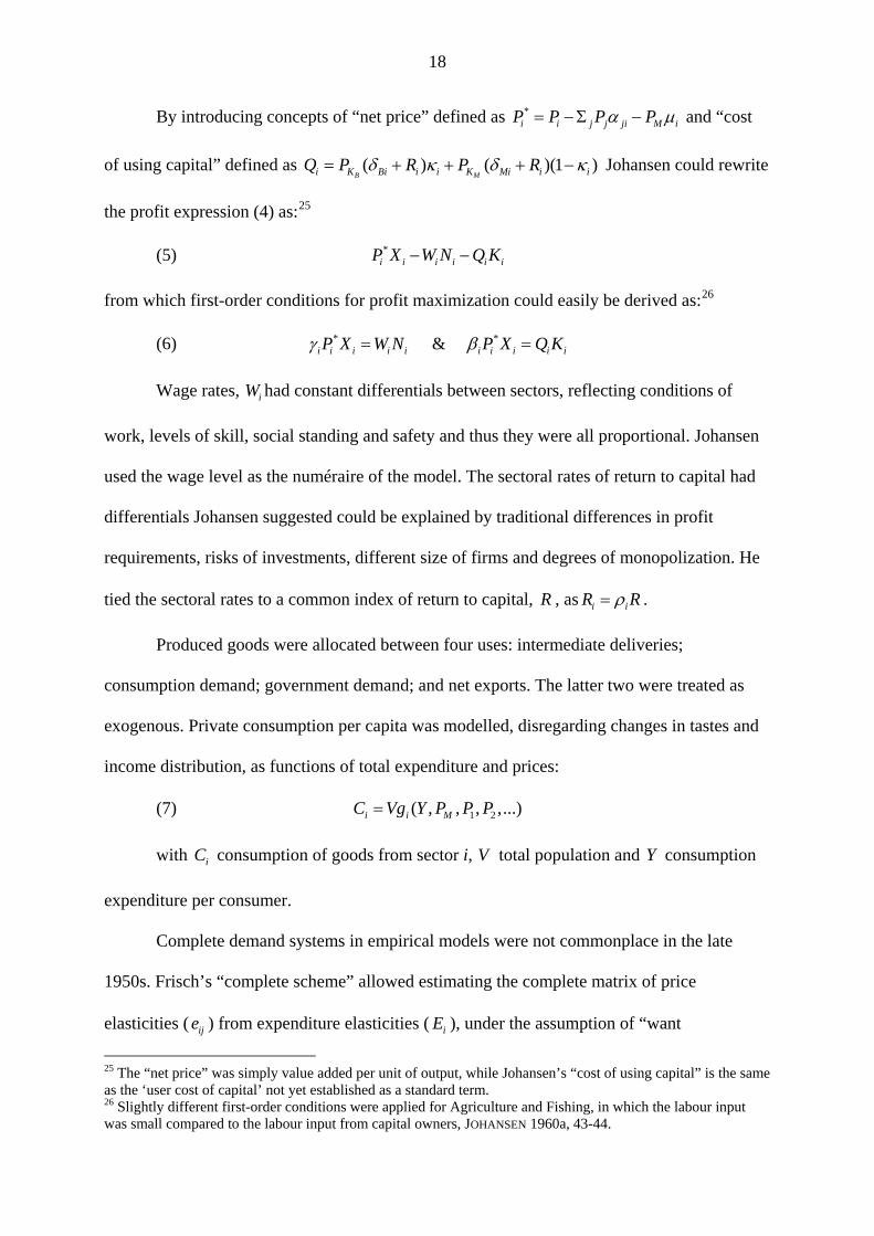
By introducing concepts of “net price” defined as *i i j j ji MP P P P iα μ= −Σ − and “cost

of using capital” defined as ( ) ( )(1 )B Mi K Bi i i K Mi i iQ P R P Rδ κ δ= + + + −κ

i

Johansen could rewrite

the profit expression (4) as:25

(5) *i i i i iP X W N Q K− −

from which first-order conditions for profit maximization could easily be derived as:26

(6) * * & i i i i i i i i i iP X W N P X Q Kγ β= =

Wage rates, had constant differentials between sectors, reflecting conditions of

work, levels of skill, social standing and safety and thus they were all proportional. Johansen

used the wage level as the numéraire of the model. The sectoral rates of return to capital had

differentials Johansen suggested could be explained by traditional differences in profit

requirements, risks of investments, different size of firms and degrees of monopolization. He

tied the sectoral rates to a common index of return to capital,

iW

R , as i iR Rρ= .

Produced goods were allocated between four uses: intermediate deliveries;

consumption demand; government demand; and net exports. The latter two were treated as

exogenous. Private consumption per capita was modelled, disregarding changes in tastes and

income distribution, as functions of total expenditure and prices:

(7) 1 2( , , , ,...)i i MC Vg Y P P P=

with consumption of goods from sector i, V total population and Y consumption

expenditure per consumer.

iC

Complete demand systems in empirical models were not commonplace in the late

1950s. Frisch’s “complete scheme” allowed estimating the complete matrix of price

elasticities ( ) from expenditure elasticities ( ), under the assumption of “want ije iE

25 The “net price” was simply value added per unit of output, while Johansen’s “cost of using capital” is the same as the ‘user cost of capital’ not yet established as a standard term. 26 Slightly different first-order conditions were applied for Agriculture and Fishing, in which the labour input was small compared to the labour input from capital owners, JOHANSEN 1960a, 43-44.

19

independence.” Frisch adhered to a cardinal interpretation of utility functions. Within a

standard framework of maximizing the utility of n goods, 1( ,.... )nu u x x= , under the budget

constraint, j j jy p x= Σ , with the marginal utility of good i defined as /iu u ix= ∂ ∂ , the budget

share of good i as /i i ip x yα = , and the marginal utility of income as /u yω = ∂ ∂ , Frisch

defined the utility acceleration of good i with respect to good j as ln / lnij i ju u x= ∂ ∂ and the

elements of the matrix 1

ij ijx u−

⎡ ⎤ ⎡ ⎤=⎣ ⎦ ⎣ ⎦ as want elasticities, i.e. the elasticity of good i with

regard to price j under constant ω .27 Furthermore, Frisch defined the money flexibility as

ln / ln yω ω= ∂ ∂ . The assumption of “want independence” is that the utility function is

additive, hence ( i ) as well as 0iju = j≠ 0ijx = ( i j≠ ) and it can be shown that /ii ix E ω= .

The price elasticities can be expressed as:

i j jij ij i j

E Ee x E

αα

ω= − − simplifying under want independence to

( 1) for

1( ) for

ji j

ijj j

i j

EE i

eE

E i

αω

αα

ω

⎧− + ≠⎪⎪= ⎨ −⎪

j

j− =⎪⎩

All price elasticities can thus be calculated from expenditure elasticities and the money

flexibility (or one direct price elasticity can eliminate a guesstimate of the money flexibility).

Johansen adopted the “complete scheme” and reparametrized it to ease the empirical

estimation. Although not necessary for his application, Johansen embraced a cardinal

interpretation as “more convenient if one is to attempt an appraisal of the realism of the

assumption of independent utilities Johansen (1960a, 88).28

27 Cf. FRISCH 1959, 181. Frisch’s “want elasticities” have later become known as ‘Frisch elasticities’. 28 Although derived under cardinality the complete scheme can be applied in an ordinal interpretation. Also others defended cardinalism in empirical work: “For empirical work … the behavioral scientist will make many assumptions analogous to cardinal measurement, and indeed to highly specific forms of cardinal utility, simply because they are usable for empirical work”, ARROW 1958, 9.

20

Johansen’s model specifications included the classical general equilibrium maximizing

assumptions in an attempt at describing the long-term pattern in the development of the

Norwegian economy. Labour and capital were assumed to be perfectly mobile between

sectors, a bold assumption taking into consideration that he aimed at depicting the growth

tendencies of the Norwegian economy in 1950, a time of post-war austerity, rationing, trade

restrictions and regulations. Few others might have thought that a general equilibrium

approach would have been the most appropriate choice. Johansen further decided to let the

marginal requirements apply with no lags or frictions.

Then came the non-trivial question of the endogenous/exogenous specification. With

reference to FRISCH (1950) Johansen made a passing remark that “one cannot, of course, say

that a model is better the more variables that are treated as endogenous. That depends on the

possibilities of establishing reliable relationships and on the purpose of the model – whether it

is designed to be a pure prediction model or a model built for planning purposes” Johansen

(1960a, 17, fn.3).

Johansen closed the model by assuming population (labour force) exogenously given

and full employment of labour.29 Johansen noted that whether full employment was possible

for a capitalistic country with a high volume of foreign trade was a formidable problem, but

on the other hand he saw “no reason why man should not be able to provide institutional

conditions which would secure a continuous and balanced growth process with full

employment of both labour and capital equipment,” Johansen (1960a, 19). His reference to

the Soviet Union as having proved that such a growth process was possible, may not have

convinced everyone. The 1950s was a period with very little growth in overall employment

but with massive transfer between industries, particularly from agriculture into manufacturing

29 This ruled out that the model could have anything to say about unemployment, the key political issue of the day, (and also disregarded any interaction between the economic development and the aggregate labour participation ratio).

21

and services. Johansen (1958a) had pointed to the role of wage differentials in the movement

of labour between industries but it was not elaborated in the model.

The other major closure assumption was that total investment was exogenous.

Johansen offered alternative justifications, either a lack of any reliable investment theory, or

that the rate of investment was controlled directly or indirectly through economic policy.

Johansen’s source for an adequate investment theory was Haavelmo’s theoretical framework

known from recent lectures. Johansen seemed to have found it attractive as a source for

investment relation as: “…being derived from an assumption of rational behaviour, and it

might seem reasonable to assume that the actual development will not over a long time

deviate systematically from that which rational behaviour dictates” Johansen (1960a, 31), but

left it at that.30

Also rates of technical change were exogenous. Johansen expressed sympathy for the

idea in Leibenstein (1957) of a relationship between income/consumption and the productive

ability of man, but finding this and other approaches toward endogenous rates of technical

progress “beyond the reach of precise and quantitative analysis” Johansen (1960a, 22).31

In his empirical model Johansen made the assumption, later adopted by many

followers, of starting from a base year, presumed in equilibrium. The base year was chosen as

1950. Most of the coefficients of the models were determined from base year data.

The non-linear equations system that emerged from the relations when put together

was not within reach for a direct solution by any computers accessible at the time. Johansen

reformulated the model by differentiating through with regard to time and defining the growth

rates in the base year as new variables. The linearized system could be written simply as

B Lξ η= and solved as 1B Lξ η−= with ξ a vector of the growth rates of 86 endogenous

variables and η a vector of growth rates of 46 exogenous variables.

30 RATTSØ 1982 gives an illuminating discussion of alternative closures of the Johansen model. 31 The specification of international trade may be considered a less developed point in the model.

22

The 86 equations comprised four equations for each sector representing: (1) the first-

order conditions for capital; (2) the weighted sum of growth in demand components to equal

production; (3) the adding-up of growth in cost components to equal growth in price; and (4)

the growth equation i i i i ix n k iγ β ε− − = (with , ,i i ix n k the growth rates of , ,i i iX N K ).

The solution of the model thus required the inversion of an 86 by 86 matrix.. This was

done by the only computer in Norway at the time.32 Although Johansen solved the model only

in terms of the growth rates in the base year the procedure suggested solving for a trajectory

by stepwise linearization. Johansen’s grip on the solution procedure was admirable. He had

been trained also in this regard at Frisch’s Institute, a place with considerable expertise in

numerical calculations.

The painstaking effort at empirical estimation of coefficients and exogenous variables

went far beyond mere numerical illustrations, Johansen indeed stated “the quantitative

analysis does no [sic!] solely serve the purpose of illustrating a method … the numerical

results also give a rough description of some important economic relationships in the

Norwegian reality.” And further: “if I were required to make decisions and take actions in

connection with relationships covered by this study, I would (in the absence of more reliable

results, and without doing more work) rely to a great extent on the data and the results

presented in the following chapters.” (JOHANSEN 1960a, 3).33

While the model itself after all had a simple theoretical structure it is not least

Johansen’s many side remarks (helpful for those who followed in his track) that showed his

mastery of the task. He commented e.g. upon how inventories and working capital (neglected

in the model) could be handled in an extended model, how new products could be handled,

how non-neutral technical progress could be incorporated, etc.

32 The computer, named Frederic, belonged to the Norwegian Defence Research Establishment. It was a Ferranti computer of Mercury type. 33 Johansen may thus be seen as a founder of an “applied model” tradition, rather than the empirically somewhat dubious “stylised model” school, flourishing within the CGE tradition, cf. DEVARAJAN and ROBINSON 2005.

23

Of more profound interest are Johansen’s remarks on the interpretation of the results

of the model, assuming that we can consider the real word as a development generated by a

complete stochastic dynamic system (Johansen 1960a, 57-59). Here Johansen draws on

concepts and ideas from Frisch’s business cycle analysis, Haavelmo’s economic evolution

essay and investment theory, and the recognition that economic data are passive observations,

which both Frisch and Haavelmo was deeply concerned with. Johansen’s remarks are brief

and almost cryptic. We cannot pursue the underlying topic here, only note Johansen’s concern

with penetrating issues of modelling methodology in the midst of dealing with the practical

details of calibrating the model.

At the very end Johansen commented upon what could be said about the optimality

character of the model results. He remarked that “it is justified to say that a development path

satisfying the equations of our model is not necessarily an optimal one, even though the

model is characterized by marginalistic adaptations. On the other hand I think that an optimal

expansion pattern can be described within the formal framework of the model” Johansen

(1960a, 172). This would hardly satisfy Frisch, whose conception of optimality required a

well defined target (preference function) and clearly defined policy instruments.

Did the empirical results shed some light on the hypothesis of sectoral employment

growth rates being determined by income elasticities? One reviewer of Johansen (1960a)

summarized the results: “Johansen shows convincingly that income elasticities are often

outweighed by the combined effects of differences in productivity, factor intensity, trade

patterns, and price changes in determining the sector distribution of employment.” (CHENERY

1961, 122).

6. Frisch’s views on the Johansen model

The committee evaluating Leif Johansen’s dissertation, comprising Frisch and Haavelmo

among its members, submitted its very brief report in October 1961. The report was drafted

24

by Haavelmo and accepted without changes by the other members. The report deemed the

dissertation “to be essentially of econometric nature, albeit the element of mathematical

statistics perhaps is somewhat less than usual in econometric studies.” It expressed no doubts

about scientific quality of the dissertation, but noted that the “explicit conclusions drawn

about the Norwegian economic growth process can be contested, partly because the available

data unfortunately have large uncertainty margins, and partly because some of the model’s

simplifying assumptions may be almost impossible to verify.”34

While Haavelmo had drafted the one-sentence reservation about the dissertation in the

evaluation report, Frisch may have had other concerns about Johansen’s endeavour. Frisch

was the modeller par excellence. He may have cared less about the availability and quality of

Norwegian statistical data being up to the model’s use of them or about assumptions difficult

to verify and more about the type of model constructed and how it could possibly fit into a

policy context. He opened anyway his opponent statement by declaring that he had never been

more convinced than in this case that the dissertation had to be accepted.35

Frisch held strong views on the meaningfulness of modelling. An ‘on-looker model’

could be constructed at any level of sophistication, but was it worth doing? The

econometrician’s imperative was to solve economic problems at national and international

level and that called for ‘decision models’.

Johansen’s competitive market assumptions bothered and confused Frisch, who

disagreed with the usefulness of making Johansen’s assumption about free mobility of labour

and capital, as being not contrary to the actual situation in Norway but, worse than that,

contrary to a proper decision point of view. Johansen referred explicitly to Friedman (1953)

for the ‘as if’ justification for the profit maximizing behaviour of producers. Frisch was hardly

34 Letter of 13 October 1961 addressed to the Faculty of Law from Ragnar Frisch, Trygve Haavelmo and Fredrik Lange-Nielsen, see THALBERG 2000, 122-123. Excerpt translated by the author. 35 The following remarks draw on notes by Frisch scribbled in the margin of his copy of JOHANSEN 1960a in preparation of the defence and notes written down during the defence.

25

prepared to go along with Friedman’s hard-boiled positivism, neither was he inclined to

accept the virtues of Soviet planning with regard to full employment and balanced

development as extolled by Johansen.

Frisch pondered over the idea of ‘balanced’ growth that Johansen claimed for his

solution. What was the nature of this ‘balance’. The closure of the model with regard to total

investment was a key point. Either one of Johansen’s two alternative interpretations, set out

above, meant to Frisch that he shied away from the essential planning problem, namely how

to make the choice between alternative investments. Had Frisch’s brightest student really

failed in understanding what a decision model was? Or did Johansen just meant to construct a

‘selection model’ as different from ‘implementation model?

Johansen had defended his choice of exogenous total investment by arguing that

investment was directly and indirectly by economic policy. At the same time he maintained

that there was a relationship based on rational behaviour between the investment and the

interest level (disregarding short term fluctuations) given by the model’s first-order condition

for profit maximization with regard to capital, interpreting the general level of return to

capital (R) as the generalized rate of interest (including a risk premium). Here he referred of

course to Haavelmo. Frisch had difficulties figuring his out and as far as he understood

Johansen’s view it run ran counter to Frisch’s way of thinking. If this was the idea, why then

was the policy not made explicit in the model: “The fact that it is not, is a clear indication that

this is no planning model, only a growth model as the title states.”36

One of Johansen’s overall simplifications in the model structure was no lags in any

relation. Frisch was puzzled over this as with no lags and exogenous investment the model

would be without any truly dynamic elements. What was then left of an explanation of

economic growth? Isn’t growth exactly that one situation ‘grows out’ of the preceding one?

36 Handwritten marginal note by Frisch on page 30 of his copy of JOHANSEN 1960.

26

Thus Johansen’s assumptions of profit maximization, factor mobility and competitive

factor remuneration may have been less palatable to Frisch, who since the depression had an

ingrained scepticism towards market prices as a functioning and efficient mechanism. Frisch

was also unenthusiastic about some of Johansen’s simplifying specifications. On the demand

side Johansen adhered to Frisch’s approach, but on the production side the use of Cobb-

Douglas functions did not arouse any enthusiasm from Frisch.37 He surely held himself as

quite an authority on production functions. In a marginal note Frisch suggested that the

exponents of the Cobb-Douglas functions at least ought to be functions of time.

Frisch’s reaction to Johansen’s endeavour was a curious mix of high admiration and a

lack of recognition of the importance of Johansen’s pioneering work for turning the general

equilibrium into an operational tool.

7. Concluding observations

Leif Johansen was an exceedingly gifted economist, not least in his ability to deal with

complicated analytic models. The characteristic feature of the seminal model of Johansen’s

dissertation was, however, not the complexity of the model but rather the parsimony of the

analytic structure that Johansen decided to work with to make sure that he would be able to

complete the model within the confinements of data availability and computing capacity.

We have above discussed Johansen’s research environment as a young scholar and his

choice of topic as the outcome of a search for an intellectual challenge. His focus on growth

may have been influenced by Haavelmo, his more specific choice of a multi-sectoral

modelling study had links to the training he had received as assistant for Frisch on input-

output analysis. Although the model he specified was not rooted in Frischian thinking the

methods and techniques he had at hand were imbued with the Frischian approach.

37 Frisch, who was present at the AEA meeting when Charles J. Cobb and Paul Douglas presented their paper in 1927, seemed never to have liked the CD-function very much.

27

Johansen’s model took as given total investment, growth in population, growth in

productivity, and changes in exogenous demand and explained from these assumptions the

change in total production, the change in employment, investment of each production sector,

and changes in relative prices, assuming market forces at work. The model was detailed and

formulated with great ingenuity to allow a numerical solution. It is a paradox, however, and

left to be explained, why Johansen (1960a) never used the term ‘general equilibrium’.

Despite Frisch’s scepticism the long-term model that originated in Johansen (1960a)

turned out to become a very useful tool. Although the history of CGE models has not yet been

written, it seems to be a fact that Johansen (1960a) exerted considerable influence upon the

early generation of CGE modellers. This was in fact foreshadowed by Hollis Chenery who in

a review of Johansen’s book in Kyklos found it “one of the most interesting and ingenious

econometric studies of recent years” and “a gold mine of new ideas for both the

econometrician and the student of economic development.” (CHENERY 1961, 121&123).38

Johansen’s book was very prominently published as issue no. 21 in North-Holland’s

Contributions series, edited by Jan Tinbergen. The book was reprinted in 1964 and came in a

second enlarged edition (see below) in 1974.

We cannot pursue here how the influence spread from Johansen (1960a) to early

pioneers and long-time practitioners in the dynamic field of CGE modelling, such as Lance

Taylor, Sherman Robinson, Peter Dixon and others, and how the theoretical specifications and

the range of applications developed. That will surely be covered sooner or later in a history of

CGE modelling. The first application of Johansen’s model, apart from the experimental

exercise in the book took place in Norway as the Norwegian Ministry of Finance invited

Johansen to develop at the Institute a second version to be used for long-term projections and

policy analyses. The model was later taken over by Statistics Norway and has continued to be

38 Other international reviews were by V. Mukerji 1963 (Econometrica 31, 770-771) and Edward Zabel 1962 (Economica 29, 284-299).

28

used as an important policy tool, cf. BJERKHOLT 1998. While long-term analyses have been

faded out in several countries as of little policy relevance the intertemporal constraints

implied by the Norwegian oil wealth have perhaps made such long-term analyses more in

demand for policy purposes in Norway than for most other countries. The Johansen model (in

successive versions) approaching a fiftieth anniversary has in any case got an unusual long

life.39

Johansen (1974), the second enlarged edition, differed from Johansen (1960a), only by

an additional long chapter of close 100 pages. Johansen surveyed “different approaches to the

study of the parts played by various sectors, and the interrelationships between them, in a

growth process.” (JOHANSEN 1974, 174). He noted the vast increase in multi-sectoral studies

since 1960. He further reported on attempts to test the model and the applications it had been

used for by the government. Then he further discussed various methodological problems that

had arisen in the use of the model and/or had been illuminated in recent literature, related to

consumption demand structure, input -output coefficients, and return to capital. Also in this

chapter there was ample guidance for new practitioners. Johansen’s work directly influenced

the development of similar models in Sweden and Denmark before CGE models became a

booming worldwide business.

Of particular interest is the link to the Australian ORANI project (DIXON et al. 1982)

which not only adopted the model idea but also was inspired by Johansen’s linearized solution

system, calling it the ‘Johansen method’. In the ORANI model the linearized solution system

was interpreted as a system of first-order differential equations giving the rates of change in

the endogenous variables as functions of the rates of change in the exogenous variables. The

system of differential equations could then be solved by conventional numerical integration

39 The current version of the successor model to JOHANSEN 1960a is MSG6, cf. HEIDE et al. 2004.

29

techniques such as the Euler procedure, see DIXON et al. (1982, 5-6).40 A further refined

version of the ‘Johansen method’ is today used by many CGE modellers all over the world

(under a different trade name).

References

ARROW K. J. 1954, “Import Substitution in Leontief Models”, Econometrica 22, 481-492.

ARROW K. J. 1958, “Utilities, Attitudes, Choices: A Review Note”, Econometrica 26, 1-23.

ARROW K. J. 2005, “Personal reflections on applied general equilibrium models”, in T. J.

KEHOE, T. N. SRINIVASAN and J. WHALLEY (eds.) 2005, 13-23.

BJERKHOLT O. (ed.) 1995, Foundations of Econometrics. The Selected Essays of Ragnar

Frisch, Two Vols., Aldershot, UK. Edward Elgar.

BJERKHOLT O. 1998, “Interaction between Model Builders and Policy Makers in the

Norwegian Tradition”, Economic Modelling 15, 317-339.

BJERKHOLT O. 2005a, “Markets, models and planning”, Memorandum No.14/2005,

Department of Economics, University of Oslo, Norway.

BJERKHOLT O. 2005b, “Frisch’s econometric laboratory and the rise of Trygve Haavelmo’s

Probability Approach”, Econometric Theory 21, 491-533.

BJERKHOLT O. 2007, “Ragnar Frisch’s Business Cycle Approach: the Genesis of the

Propagation and Impulse Model”, The European Journal of the History of Economic

Thought 14, 449-486.

BORCH K. H. 1987, “Johansen, Leif (1930-1982)”, in The New Palgrave. A Dictionary of

Economics Vol. 2, London, Macmillan, 1987, 1020-1022.

CASSEL G. 1927, The Theory of Social Economy, London, T. Fisher Unwin.

CHENERY H. B. 1961, Book review of “Leif Johansen: A Multi-Sectoral Study of Economic

Growth”, Kyklos 14, 121-123.

CHENERY H. B., P. G. CLARK and V. CAO PINNA 1953, The Structure and Growth of the

Italian Economy, U.S. Mutual Security Agency, Rome.

DEVARAJAN S. and S. ROBINSON 2005, “The influence of computable general equilibrium

models on policy”, in T. J. KEHOE, T. N. SRINIVASAN and J. WHALLEY (eds) 2005,

402-428. 40 The further refined version of the “Johansen method” is today used by many CGE modellers under the trade name of Gempack, see http://www.monash.edu.au/policy/gempack.htm.

30

DIXON P. B., B. R. PARMENTER, J. SUTTON and D. P. VINCENT (1982), ORANI: A

Multisectoral Model of the Australian Economy, Amsterdam, North-Holland.

FRIEDMAN M. 1953, Essays in Positive Economics, Chicago, University of Chicago Press.

FRISCH R. 1946, “The responsibility of the econometrician”, Econometrica 14, 1-4.

FRISCH R. 1948, “Repercussion studies at Oslo”, American Economic Review 38, 367-372.

FRISCH, R. 1950, “L’emploi des Modèles pour l’Elaboration d’une Politique Economique

Rationnelle”, Revue d’Economie Politique 60, 474-498 & 601-634.

FRISCH, R. 1952a, “Repercussion-analytical problems which can be studied on the basis of the

flow of goods and services divided by shares of input requirements, main categories of

goods, and industry sector [In Norwegian]. Professor Ragnar Frisch’s lectures in the

autumn of 1952”, (Elaborated notes prepared by Leif Johansen), Memorandum from

the Institute of Economics of 6 November 1952, University of Oslo.

FRISCH R. 1952b, “Linear programming – Report of Professor Ragnar Frisch’s lecture 15

February 1952 [In Norwegian]”, (Notes by Leif Johansen), Memorandum from the

Institute of Economics of 17 February 1952, University of Oslo.

FRISCH R. 1955, “The Mathematical Structure of a Decision Model: The Oslo Sub-Model”,

Metroeconomica 7, 111-136.

FRISCH R. 1959, “A complete scheme for computing all direct and cross demand elasticities in

a model with many sectors”, Econometrica 27, 177-196.

FRISCH R. 1960, Maxima et Minima.Théorie et applications économiques, Paris, Dunod.

FRISCH R. 1962, “Preface to the Oslo Channel Model – A Survey of Types of Economic

Forecasting and Programming”, in R. C. Geary (ed.) 1962 Europe’s Future in Figures,

Amsterdam, North-Holland, 248-266.

FRISCH R. 1965, Theory of Production, Dordrecht-Holland, D. Reidel.

HAAVELMO T. 1944, “The Probability Approach in Econometrics”, Econometrica 12

(Supplement), 1-118.

HAAVELMO T. 1949-50, “A note on the theory of investment”, Review of Economic Studies 16,

78-81.

HAAVELMO T. 1954, A Study in the Theory of Economic Evolution, Amsterdam, North-

Holland.

HAAVELMO T. 1960, A Study in the Theory of Investment, Studies in Economics, Chicago,

University of Chicago Press.

HARBERGER A. C. 1962, “The incidence of the corporate income tax”, Journal of Political

Economy 70, 215-240.

31

HEIDE K. M., E. HOLMØY, L. LERSKAU and I. F. SOLLI 2004, Macroeconomic properties of

the Applied General Equilibrium Model MSG6, Reports 2004/18, Statistics Norway.

JOHANSEN L. 1956, “The free maximum method of solving linear programming problems”,

Memorandum from the Institute of Economics of 3 May 1956, University of Oslo

JOHANSEN L. 1958a, “A note on the theory of interindustrial wage differentials”, Review of

Economic Studies 25, 109-113.

JOHANSEN L. 1958b, “Forholdet mellom næringene under økonomisk vekst: en

litteraturoversikt”, Statsøkonomisk Tidsskrift, 72, 95-118.

JOHANSEN L. 1959, “Substitution versus Fixed Production Coefficients in the Theory of

Economic Growth: A Synthesis”, Econometrica 27, 157-176.

JOHANSEN L. 1960a, A Multi-Sectoral Study of Economic Growth, Amsterdam, North-Holland.

JOHANSEN L. 1960b, “Rules of Thumb for the Expansion of Industries in a Process of

Economic Growth”, Econometrica 28, 258-271.

JOHANSEN L. 1972, Production Functions. An Integration of Micro and Macro, Short Run

and Long Run, Amsterdam, North-Holland.

JOHANSEN L. 1974, “A Multi-Sectoral Study of Economic Growth”, Second Enlarged Edition,

Amsterdam, North-Holland.

KARMARKAR N. 1984, “A new polynomial-time algorithm for linear programming”,

Combinatorica 4, 373-395.

KEHOE T. J., T. N. SRINIVASAN and J. WHALLEY (eds) 2005, Frontiers in Applied General

Equilibrium Modeling. In Honor of Herbert Scarf, Cambridge UK, Cambridge

University Press.

LEIBENSTEIN H. 1957, Economic Backwardness and Economic Growth, New York.

LEONTIEF W. 1951, The Structure of American Economy, 1919-1939, Second Enlarged

Edition, New York, Oxford University Press.

LEONTIEF W. 1953, Studies in the Structure of the American Economy, New York, Oxford

University Press.

LEWIS W. A. 1955, The Theory of Economic Growth, Homewood, Ill., Richard D. Irwin.

MORISHIMA M. 1958, “Prices, interest and profits in a dynamic Leontief system”,

Econometrica 26, 358-380.

RATTSØ J. 1982, “Different macroclosures of the original Johansen model and their impact on

policy evaluation”, Journal of Policy Modeling 4, 85-97.

SAMUELSON P. A. and R. M. SOLOW 1953, “Balanced growth under constant returns to scale”,

Econometrica 21, 412-424.

32

SCHULTZ T. W. 1945, Agriculture in an Unstable Economy, New York: McGraw-Hill.

SIMON H. A. 1947, “Effects of Increased Productivity upon the Ratio of Urban to Rural

Population”, Econometrica 15, 31-42.

SOLOW R. M. 1956, “A contribution to the theory of economic growth”, The Quarterly

Journal of Economics 70, 65-94.

SOLOW R. M. 1987, “Growth Theory and After, Prize Lecture, December 8, 1987”,

http://nobelprize.org/nobel_prizes/economics/laureates/1987/solow-lecture.html.

SOLOW R. M. 1983, “Leif Johansen (1930-1982): A Memorial”, Scandinavian Journal of

Economics, 85, 445-456.

THALBERG B. 2000, “Leif Johansen 1930-1982”, Norsk Økonomisk Tidsskrift 114, 1-157.

TINBERGEN J. 1966 [1952], On the Theory of Economic Policy, Amsterdam, North-Holland.

VON NEUMANN J. 1945-46, “A model of general economic equilibrium”, Review of Economic

Studies 13, 1-9.