the long and winding road towards optimal fiscal
TRANSCRIPT

1
The long and winding road towards optimal fiscal decentralization*
Maria Laura Alzua1
April 25th, 2005
PRELIMINARY DRAFT
Abstract This paper studies some of the difficulties which may arise in a process of fiscal decentralization. We look at an economy which has started a process of fiscal decentralization but may fail to achieve its optimum level according to Oates’ decentralization theorem. This failure may be the result of subnational governments’ fiscal irresponsibility and lack of credible commitment technology on behalf of a central government. We look particularly as dollarization as a commitment technology in order to induce discipline in subnational governments. Do incentives for Central Government bailouts disappear with dollarization? Does incomplete fiscal decentralization arises in equilibrium? We obtain two different sets of equilibria as result of a game between national and sub-national governments according to the difference parameter configuration. In one of them the Central Government will give taxing autonomy to the sub-national governments while in the other it will keep the taxing authority because it is optimal to do so. In this sense, the economy gets stuck in an inefficient level of fiscal decentralization. The model may apply to economies like Argentina, Ecuador, the CFA in Africa and Eastern European countries willing to join the Euro. JEL classification Numbers: E62, H63, H72 Keywords: Decentralization, default, taxes, sub-national governments. 1. Introduction Recent history of developing countries has focused on diverse issues concerning
monetary and fiscal policy. Given the history of monetary policy mismanagement in some countries, especially in most of Latin American ones, how to conduct it in terms of reducing inflation has been an important issue of debate both at the academic and policy making level. On the other hand, fiscal reforms appear to be a pre-condition in all stabilization plans. Tax reforms, public spending re-direction and rationalization are necessary measures to achieve an improvement in the efficiency of the public sector in order to make it consistent with a
*This project has been possible thanks to the Summer Research Grant of Boston University, Department of Economics. I want to thank Russell Cooper, Oscar Landerretche (h), Ricardo Madeira and Edgar Villa and to the participants in the Economic Seminars at UDESA, the Macro Graduate Workshop at Boston University, participants of Latin American Econometrica Meeting in Santiago de Chile, 2004. All remaining errors are mine. 1IERAL de Fundación Mediterránea, [email protected]

2
more prudent monetary policy. The bulk of reforms in order to enhance the performance of the public sector are mainly related to fiscal decentralization.
Some developing countries, especially many in Latin America, suffered from high inflation during the 80’s. This inflation resulted mainly from lack of discipline in government spending (both at the national and the state level). Tax incidence has been generally low and so large deficits were financed by printing money. Some of these countries suffered even from hyperinflation processes as a result of these policies2. In the process to reduce inflation, most of the countries adopted some form of peg for the exchange rate, which ranged from fixed exchange rates to currency boards or even dollarization.
One of the most important things that should be achieved in order to give credibility to the pegs is to design fiscal policies that should be consistent with these exchange rate regimes. Otherwise, large monetized fiscal imbalances led to a loss of reserves and a subsequent speculative attack that forced governments to abandon the pegs, as in Krugman (1979) seminal paper. In order to give credibility to the pegs, governments should reduce their budget deficits. In terms of Rebelo (1997) words’: ‘‘pegging the exchange rate tend to be associated with an increase in government efficiency in the present and in the future. This efficiency increase results from measures such as the reform of the tax system and the re-direction of government expenditures away from redistribution programs and pork barrel spending towards productive uses.’’
The task of reducing budget deficits is hard in nature, since it involves unpopular measures that are difficult to enforce in the short term. Most politicians are unwilling to pay the high costs of fiscal reforms. In this sense, fiscal decentralization aims at improving the performance of the public sector. The most widespread approach to decentralization in the public finance literature is known as fiscal federalism. It identifies three main functions for the public sector: macroeconomic stabilization, income redistribution and resource allocation. While macroeconomic stabilization and income redistribution functions are assigned to the central government, sub-national governments should be in charge of resource allocation mainly for efficiency reasons. In terms of the Decentralization Theorem: “… .in the absence of cost-savings from the centralized provision of a [local public] good and of inter-jurisdictional externalities, the level of welfare will always be at least as high (and typically higher) if Pareto efficient levels of consumption are provided in each jurisdiction than if any single, uniform level of consumption is maintained across all jurisdictions”3
Another line of reasoning in order to justify fiscal decentralization is the idea of fiscal correspondence and the common pool problem. When the provision of public goods and services is in charge of decentralized units (i.e. sub-national governments) but there is no decentralization in terms of revenue collection, the problem of fiscal correspondence appears. Individuals enjoying the benefit of consuming public goods do not bear the total cost of providing them. Moreover, the common pool problem refers to the fact that sub-national governments behave as if they did not face a hard budget constraint, increasing government spending and reducing regional tax effort.
Finally, implicit Central Government bailout assumption also acts as a dynamic relaxation of sub-national governments’ budget constraint. In order to reduce the above mentioned problems, fiscal decentralization aims at improving the efficiency of public goods
2 We can quote as historical cases of hyperinflation in the 80’s Argentina, Bolivia and Brazil. Most of the rest of Latin American countries suffered from high and persistent inflation though not hyperinflation. 3 Oates, (1972, p.54)

3
provision together with aligning incentives of public expenditure with regional tax collection effort.
Most Latin American countries have started a decentralization process of their fiscal around a decade ago. The purpose of such process was to improve the performance of their public sectors. So far, in many LA countries, whereas most of the expenditures have been decentralized, the same cannot be said about revenue decentralization. Argentina has one of the most decentralized systems (in terms of expenditures) of all Latin America. For its specific case, regional governments are in charge of most of the social expenditure (health, education, infrastructure, etc.), which accounts for 50% of all public sector expenditures are in the hands of sub-national governments. (In Brazil, this figure is 45.6% and in Colombia 39%)4. Moreover, while sub-national governments have constitutional taxing decisions, most of the regional governments have delegated its taxing authority to the national government not only for tax collection but also for setting tax rates and bases.
The imbalance between expenditures and revenues, the common pool problem and the implicit bailout assumption on behalf of the Central Government creates an incentive for sub-national governments to run irresponsible deficits, since they do not face the financial consequences of their actions.
There are different issues present in the literature that can be used to address the
problem of interaction between monetary and fiscal policy:
1. the problem of persistent positive inflation, caused when the monetary authority is not independent and the “printing press” is used to finance budget imbalances.
2. the deficit (either monetized or not) bias that results from some specific fiscal structures in some countries. Here it is important to consider the degree of fiscal decentralization/centralization of each country and the problems of fiscal imbalances generated by non-optimal decentralization schemes.
3. currency pegs, hard monetary rules and even dollarization as commitments not to finance budget deficits.
In the case of persistent positive inflation there is a vast literature that tries to
address this problem. We will not focus in the literature related to credibility of the monetary policy. An excellent account of the evolution of this literature can be found in Persson and Tabelini (2000). First, we will address the problem of inflation as a direct consequence of fiscal indiscipline and weak commitment power of the Central Government and the Central Bank (which we will treat as the same agent.)
The second point we will address is fiscal federalism. There is both theoretical and empirical evidence –though in a lesser degree- which supports the improvement of economic efficiency in the public sector by means of fiscal decentralization. Oates (1999) presents all the theoretical conditions for which both revenue and expenditure decentralization might be optimal. In terms of empirical evidence, we observe that an important group of countries spanning Europe, Asia, Africa and Latin America are undergoing a process of devolving fiscal responsibilities to their sub-national governments. Whereas each country presents differences in this process, a common feature can be 4 For more details about this see Piffano (1998) and Tommasi, Sanguinetti and Saiegh (2001)

4
observed. Most of the countries have given back expenditure responsibilities without the accompanying revenue raising responsibilities. As we mentioned before, both the lack of fiscal correspondence and the implicit bailout assumption often create perverse incentives for sub-national governments which cause too much deficits and too much borrowing. Among the main reasons for an implicit bailout assumption we can quote a country’s political configuration (the Central Government often needs political support from sub-national leaders) and externalities (“too big too fail” argument, where an important sub-national government in problems becomes a problem for the Central Government) Here, Garcia Mila, Goodspeed and McGuire (2001) analyze the case of fiscal decentralization in evolving federations. They develop a theoretical model of regional borrowing decisions in which the incentives for regional borrowing depend on the regions’ expectations about the federal system of finances is going to evolve. Their results suggest that if taxing authority is given back to the regions, then sub-national borrowing can efficiently correct any initial revenue deficiency. But, if regional governments expect the central government to increase grants as a response to increase in regional borrowing, then a “soft budget constraint” is created and there is a tendency to too much borrowing. Here, the decision of taxing autonomy and the perception of softness in the CG budget constraint appears as exogenous. It is important to achieve some explanation of why central governments may be reluctant to give taxing authority to regional governments or why regional governments have no incentives to claim taxing responsibilities.
Finally, one of the main points for dollarization5 (or currency boards) in one country is the idea that by delegating the monetary policy to another country the delegating country can achieve significant reduction in inflation. The most recent examples are Argentina and Ecuador in the nineties. The literature supporting dollarization is abundant. But the main line of reasoning behind dollarization can be summarized as follows:
There is a Central Government (CG) who likes to use the ‘printing press’ in order to finance current expenditures. The Central Bank (CB) is usually weak and finances government deficits. This causes inflation and all the accompanying problems that it brings. In this sense, dollarization or currency boards represent a commitment to stop the ‘printing press’, and this will reduce inflation.
Another line of reasoning, which appears in Cooper and Kempf (2001), enhances the previous analysis by complicating the political structure of the inflation-prone countries. In this case, there are regional governments (RG) who can exert pressure on a weak CG by asking them to monetize its deficits. Here, a multiregional model is used, where many regions would like the CG to monetize its deficits, since the burden of the inflation tax would be borne by other regions. The equilibrium in this model is of a positive inflation.
In both types of models, what appears to be crucial is the lack of credibility of a commitment of the CG not to run deficits at the national level or to bailout fiscally irresponsible regions. The question is: is dollarization enough of a commitment when the CG is susceptible to pressures from the regional governments? Regions will still have incentives to run deficits that will imply higher taxes in the future. So the CG should have to raise taxes in all regions, and the burden of higher taxes will be suffered for all. In terms of Copper and Kempf (2001) words: “The core of the monetary problem is fiscal irresponsibility, not the choice of currency”
The present study is aimed at analyzing two things: first, which are the different economic configurations that may give rise to a sub-optimal level of decentralization in a 5 Here we are ignoring all the potential beneficial effects of dollarization on trade.

5
federal country and the role played by dollarization as a commitment to impose fiscal discipline in a federation.
We will explore different commitment mechanisms for the Central Government (CG) not to bail out sub-national governments (RG). Can the Central Government and the regions sign a contract to reduce the Central Government bailouts? Dollarization, per se, rules out monetization of regional deficits but this does not means that CG bailouts disappear. The Central Government can still bail out regional governments by means of higher taxes. i.e.: CG raises taxes to rescue regions running deficits.
Why is that some Central Governments find it so hard to push reforms in terms of revenue decentralization once they had given expenditures decentralization?
In order to make an attempt to answer such question, we develop a model to study the interaction of CG and RGs in the context of a dollarized economy. We model two different situations: first, one economy which has random endowments. We look for the Weak Perfect Bayesian Equilibrium of the game between the Central and the Regional Government. The CG has to decide whether to give taxing autonomy to the regions or not. In this first case, only one RG is active. We look for the Weak Perfect Bayesian Equilibrium, restricting ourselves to pure strategies. We obtain different sets of equilibria. There are different configurations of parameters which support different choices for each level of government (endowment volatility, size of the region and the distribution of debt holdings). We are interested in looking at the set of beliefs and strategies that give rise to the regional taxation equilibrium and to the equilibrium without fiscal decentralization. The former is the most efficient in terms of the decentralization theorem and reduces the deficit bias observed in regional governments. The latter is of interested since many of the countries undergoing decentralization processes get “stuck” in this intermediate phase of fiscal decentralization. It is worth looking at which configuration of parameters give rise to this equilibrium. Also, this equilibrium suggests that dollarization does not eliminate CG bailouts and so it is not enough as a commitment to induce fiscal discipline in the regions. Secondly, we repeat the game allowing for regional interaction. We look for the Sub-game perfect Nash equilibrium, since as we will show, random output plays no restrictions on beliefs, and so, with the objective of simplifying the inter-regional game, we have eliminated it.
The paper is organized as follows: section 2 presents a model of CG and one RG interaction with uncertainty over output. Section 3 extends the game to allow interaction between RGs and the CG. Section 4 provides some explanation of why the model could be applied to Argentina and some policy implications. Section 5 concludes.
2. A real game between CG and RG. Here, we develop a simple two period model to study an economy with the
following characteristics: - The CG has no monetary policy, and has to look for other ways to finance
national or sub-national budget deficits. - The country is in the middle of the process of fiscal decentralization,
expenditures are decentralized at a regional level but revenues are still centralized6.
6 We assume this type of decentralization because it has been observed empirically. The first step towards decentralization has been generally expenditure decentralization, followed only later by revenue decentralization. For a detailed survey about this issue see Freire, Huertas and Darche (1998).

6
The economy is populated by N identical agents who live for two periods. There is a
Central Government (CG) and two regions (R1 and R2), each with its own government (RG1 and RG2). Population in each region is N1 and N2, they may not necessarily be equal. The CG has no control over monetary policy. Expenditure policy is determined at the regional level7. There is no production. Agents have endowments in both periods. While there is certainty in period one endowment, period two endowment is random. In period one CG makes transfers to the provinces g. Following Mila et al. (2000) we consider these transfers of period one to be exogenous and assume that there is a mismatch between g, and RG spending in period one in order to introduce RG’s borrowing or lending as in McGuire et al. (2001)8.
The model captures two different things: one, given the fact that we are in a context of an economy without monetary policy, so CG cannot bail out the RG by means of printing money, and second, the country is in an early stages of reform in terms of fiscal federalism, i.e.: while RG have spending responsibilities, they have not taxing authority yet. The timing of the game is as follows:
Stage one:
• CG sets exogenous transfers to the provinces and decentralizes expenditures • RGs issue bonds bi to finance the gap between CG’s transfers and desired
spending. • All young agents make decisions in anticipation of period two government
policies
Stage two: • Regional governments observe the realization of endowments Yh or Yl (high
and low endowment respectively)9. • CG decides to give taxing authority (TA) to RG or not (NTA). • If CG gives taxing authority to RGs, RGs can choose to levy the tax (TAX)
or pass the obligation to the CG (NO TAX). • CG can choose to bail out (BO) (by means of economy wide tax) RGs. • If CG does not levy an economy wide tax, RGs will default (D), paying a
penalty costδ. • If CG does not pass the taxing authority (NTA) to RGs then it has to bail
out (BO) RGs.
We search for a Weak Perfect Bayesian Equilibria (WPBE) of this game. The CG cannot make credible threats not to bail out RGs. We will analyze the equilibria when the CG lacks this commitment power. For simplicity, only RG1 is active, RG2 has no mismatch between CG grants and its expenditures. We can think, for example, that RG2 had
7 We are in a context where the country that can be characterized as an “evolving federations” in the terms of McGuire et al. (2001). CG gave spending but not taxing responsibilities to RGs. 8 In this point we follow McGuire et al. (2001). 9 At this point we consider the realization of endowments is the same for both regions. This can be modified.

7
borrowing restrictions in its constitution. The tree corresponding to this game can be seen in the appendix.
Individuals live for two periods where the superscripts “y” and “o” stand for young and old respectively. 2.1 Period 1 Optimization
Individuals derive utility from consumption of a private and public good. Region i young agents solve:
),(),(,
oi
oi
yi
yi
bb
gcEugcumaxij
ii
β+ , for i=1,2 (1)
where u is assumed to be concave. subject to:
yi
iyi Ybc =+ (2)
iyy
i bgg += (3)
)()1()( oiii
oi YEbREc ττ −−+= (4)
TYEbREgg i
oiii
yoi ητ ++−= )()( (5)
j
iiii bbb += (6)
where: All the variables are expressed in per capita terms
yg is real per capita transfer in youth to agents of region i og is real per capita transfer when old to agents of region i y
iY is endowment in youth
)( oiYE is endowment in old, which is random
ib , debt held by region i j
ib is debt issued by region i held in region j
iτ is a regional tax τ is a common tax collected by the Central Government

8
]1,0[∈iη is a parameter that will indicate how much of the total tax is
redistributed back to the regions. Endowment is random and takes two values high or low with probability p and (1-p)
respectively. Here iη is going to be equal to one, i.e.: there is no difference between transference
to regions. Per capita transfers are equal across regions.
R is the return on holding regional Government debt and are considered to be
exogenous10, taking two values: hR when output is high and hl RR α= , with 10 <<α . Given some initial conditions, this maximization problem is well defined and has explicit solutions for consumption and regional government debt holdings for some parametrical assumptions about the utility functions. The first order conditions for this problem are:
:)( iib ))]('())('([)(')(' o
ioi
yi
yi gRuEcRuEgucu −=− β (9)
:)( ijb ))('()(' o
iy
i cRuEcu β= (10)
The LHS of (9) is the marginal cost of giving up consumption today. In this sense, increasing public good consumption reduces this marginal cost. The RHS represents the marginal benefit of consumption tomorrow. From (9) and (10) we obtain:
))]('()(' oi
yi gRuEgu = (11)
and )()(')('
)(')('
REgugu
cucu
oi
yi
oi
yi == (12),
which is the standard intertemporal efficiency relationship between present and future consumption for private and public goods. Here, agents are able to smooth private and public good consumption, achieving intertemporal efficiency, but, due to the lack of regional taxation in period one, intratemporal efficiency is not achieved. Issuing regional debt does not correct for initial mis-funding of regional governments.11
10 In our simple setting we just consider R to be exogenous but positively correlated with endowments. This result appears in the literature, and it can be justified as follows: we can think of a closed economy, operating near full capacity, with adjustment costs to increase the stock of capital in the short term. Any positive shock will push up marginal productivity of capital, until investment is fully adjusted, showing procyclicality of interest rates. 11 This is the same result obtained in Garcia Mila et al. (2000)
∑=
=2
1iiYT τ

9
2.2 Period 2 payoffs
In order to consider the second period payoffs we make some simplifying assumptions. First, we will start by assuming a linear utility function yy ccu =)( and 00 =g , which means that in equilibrium, bbb == 21 . Finally, CG transfers in period two will be equal to zero.
RG1 government is concerned with the welfare of its citizens. The CG government takes into account the welfare of both regions in the following way: the objective function of CG is the population-weighted sum of the utilities of each region’s agents plus Π, which represents autonomous CG consumption. We can write the welfare function of CG as follows:
γ−Π+∆−+∆= ooCG ccW 11 )1( ,
where ∆ and )1( ∆− are the population weights of R1 and R2 respectively, and Π is autonomous government consumption. The term γwill be different from zero only in the case that the CG has to bailout RG1 once it has taxing autonomy. This can be understood as an “extra effort” on behalf of the Central Government once it has given taxing authority to the regions. We are going to consider γ as fixed, but in a more complicated environment, it can be made a function of τ , the tax rate, the higher the tax rate, the higher the reduction in CG consumption. For the CG, the welfare of a CG bailout will then decrease, the higher the level of regional debt. 12
We are going to analyze the case where endowments shocks are perfectly correlated and equal across regions. The rationale given for saying that the realization of output is observed by RG and not CG comes from the fact that in general RGs have much more information about the productivity and the real possibilities of their economies than the CG. We have a principal agent problem, where it is costly for the CG to monitor the activity in the regions. We will write in turn the different payoffs for each state of nature. A complete derivation of payoffs can be seen in the appendix
2.2.1 CG gives taxing autonomy and RG1 taxes its citizens.
This payoff corresponds to the state where complete fiscal decentralization is achieved. This is the “good equilibrium” in terms of the decentralization theorem. Here R1 individuals will bear the full cost of repaying period one debt. This equilibrium will be the one “preferred” by R2 individuals.
Payoffs when endowment is high:
hho YbRc )1( 1
11 τ−+= (11) and
∆∆−+=
21
1)1( b
bRY hhτ (12)
12 In the context of tax decentralization, the CG loses sources of revenues and so it has to resort to reduce its consumption in order to finance the regions.

10
combining (11) and (12) we obtain:
∆∆−−==
2
1)1( bRYcW h
hoRG (13) for RG1 citizens
hCG YW +Π= for CG (14) which are the welfare functions of the regional and central government respectively. Payoffs when endowment is low:
When endowments are low, return on regional debt is hl RR α= .α ranges between zero and one 10 <<α , is the default rate, i.e. a low realization of endowment means partial default on period one government debt. If α =1, debt can still be repaid when endowment is low. If this is the case, uncertainty over endowments plays no role over the beliefs on the players. Incomplete information on behalf of the CG plays no role in determining the different equilibrium of the game.
By introducing default risk, we will be able to look at two different things: -the role of endowment volatility as a parameter which affects the result of
the game. -the role of informational asymmetries between CG and RG, in the sense
that the latter knows the state of the economy before than the former.
∆∆−−==
2
1)1( b
RYcW hl
oRG α (14) for RG1 citizens
lCG YW +Π= (15) for CG
Regardless of the realization of endowments, ex-post consumption in R1 is lower the higher the proportion of debt held in R2. R1 individuals bear the tax burden to repay the debt held in R2. This will produce an analogous result to the one found in Cooper et. al., (2003), where they find an equilibrium with regional taxation when debt is held just in R1. As we will see later, debt holding distribution matters for the equilibrium that is chosen.
2.2.2. CG gives taxing autonomy and RG1 does not tax and CG bails out RG by means of higher taxes Payoffs when endowment is high:
21 bRAyW hhRG
∆∆−−= , for RG (16)
where
∆∆−+∆= )1(τA ,

11
hCG yW +−Π= γ , for CG (17)
Payoffs when endowment is low:
21 bRAyW hlRG α
∆∆−−= , (18) for RG
lCG yW +−Π= γ , (19), for CG
We are assuming that CG charges an uniform tax rate is τ in both regions. Here, A is greater than one, so payoff for the RG1 will be higher than in the case of
regional taxation regardless of the level of b2. This seems reasonable, since RG2 citizens bear also the burden of higher taxation in period two. This result will be preferred by RG1 citizens, since they can enjoy higher consumption in period one and share the burden of re-paying debt with R2 individuals.
CG has the above mentioned cost γ, due to the fact that it has already given taxing authority to the regions, and so bailouts entail a higher effort that lowers CG autonomous consumption.
2.2.3 CG gives taxing autonomy, RG does not levy a regional tax, and CG allows default Payoffs when endowment is high:
δ−= hRG yW , (20) for RG1 citizens
hCG yW +∆−Π= δ , (21) for CG
Payoffs when endowment is low:
δ−= lRG yW , (21) for RG1 citizens
lCG yW +∆−Π= δ , (22) for CG
2.2.4 CG does not give taxing autonomy, bailing out RG
Here, the fiscal decentralization process is not complete. Regions do not have taxing autonomy, so the process of fiscal imbalance worsens. This creates deficit biases in region 1 and, while dollarization forbids the CG to print money to bail out RGs, the tax bailout has the same spirit than an inflation tax in a monetary economy. Dollarization does not solve any problem of fiscal irresponsibility.

12
Payoffs when endowment is high:
21bRAyW hhRG
∆∆−−= , (23) for RG1 citizens
hCG yW +Π= , (24) for CG
Payoffs when endowment is low:
21bRAyW hlRG α
∆∆−−= , (25) for RG1 citizens
lCG yW +Π= , (26) for CG
2.3 Equilibria13
We look for the Weak Perfect Bayesian Equilibrium, restricting ourselves to pure strategies. As mentioned before, we obtain different sets of equilibria. There are different configurations of parameters which support different choices for each level of government. We are interested in looking at the set of beliefs and strategies that give rise to the regional taxation equilibrium and to the equilibrium without fiscal decentralization. The former is the most efficient in terms of the decentralization theorem and reduces the deficit bias observed in regional governments. The latter is of interested since many of the countries undergoing decentralization processes get “stuck” in this intermediate phase of fiscal decentralization. It is worth looking at which configuration of parameters give rise to this equilibrium. Also, this equilibrium suggests that dollarization does not eliminate CG bailouts and so it is not enough as a commitment to induce fiscal discipline in the regions.
2.3.1. Equilibrium with fiscal decentralization and regional taxation
Proposition 1: Under the following conditions (see proof in the appendix)
δγ ∆> , (27)
21bRh
∆∆−>δ (28)
and 21bRhαδ
∆∆−> (29).
there exists an equilibrium where CG grants taxing autonomy to RG1 and RG1 taxes is citizens.
13 Please refer to appendix 1 for a detailed analysis of equilibria.

13
Whenever (28) is satisfied, (29) is satisfied too. The range of values such that CG will give taxing autonomy to the regions and RG will choose regional taxation will increase:
- as γ, higher cost of bailout once taxing autonomy has been given. -default costs are sufficiently high for the regions but not so high so as CG does not
grant taxing autonomy in the first place. -the smaller the size of R1 -Return structure of government debt Here, it’s interesting to note that output volatility does not matter for the CG to
decide to grant taxing autonomy or not. CG will grant it only when it will allow RG to default instead of bailing it out. Whenever CG prefers a bailout to a default, taxing autonomy is not granted, since CG’s welfare is higher than decentralizing. Output volatility matters only to the decision of RG whether to tax or not once taxing autonomy has been conceded.
2.3.2 Equilibrium without fiscal decentralization
Proposition 2: Under the following condition (see proof in the appendix): δγ ∆≤ there exists an equilibrium where CG wil not give taxing autonomy to RG1 Here CG always prefers not to grant taxing autonomy regardless of p. Again, output
volatility plays no role in CG decision. Low decentralization costs γmakes a CG bailout after taxing autonomy has been granted more attractive, and so CG prefers not to give taxing autonomy in the first place.
There are no restrictions on CG beliefs for which it will prefer a BO to a default. It
only depends on the fiscal cost of a BO2 with respect to the default costs in CG’s government function. This also depends on R1 population, since allowing default is more costly the bigger R1 is. Given that CG always bailout R1, then it is always the case than RG1 will not choose regional taxation, regardless of output realization. Here regional tax effort is non existent and complete fiscal decentralization will never take place.
In the case that δγ ∆> , then CG will allow R1 default. If this is the case, sufficiently large default costs will ensure RG choose regional taxation. But, as δin creases, then the set of values for which CG allows default is reduced, unless the R1 is sufficiently small. Whenever default costs are relatively high to R2 debt holdings, then there is an equilibrium with regional taxation and a positive level of debt. Regional taxation also depends on α . If α is low, then the cost of regional taxing becomes smaller, and RG1 will tax its citizens when output is small.
3. A real game of regional interaction. While the simple model presented in the previous section where only one region is
active sheds some light about why a country may end up in a process of incomplete fiscal decentralization, it is useful to study what happens when regional interaction is taken into account. Here we present a model where two regions (RG1 and RG2) interact while CG must decide whether to grant taxing autonomy or not to regional governments. In order to

14
simplify the game studied we eliminate output volatility, since we showed it played no role in GC decision.
The case with regional interaction certainly can be applied to what was observed in Argenina before the collapse of the Convertibility regime. Regional deficits were high and regions were bailed out by CG, until CG defaulted on its obligations.
We extend the model to allow for regional interaction, eliminating output volatility and adding RG2 actions. Otherwise the model is the same than the one developed in the previous section.
Stage one: • CG sets exogenous transfers to the regions, decentralizes expenditures and
dollarization starts • RGs issue bonds bi to finance the gap between CG’s transfers and desired
spending. • All young agents make decisions in anticipation of period two government
policies
Stage two: • CG decides to give taxing authority (TA) to RG or not (NTA). • If CG gives taxing authority to RGs, RGs can choose to levy the tax (TAX)
or pass the obligation to the CG (NO TAX). • CG can choose to bail out (BO) (by means of economy wide tax) RGs. • If CG does not levy an economy wide tax, RGs will default (D), paying a
penalty costδ. • If CG does not pass the taxing authority (NTA) to RGs then it has to bail
out (BO) RGs.
We search for a Sub-game Perfect Nash Equilibria of this game. The CG cannot make credible threats not to bail out RGs. We will analyze the equilibria when the CG lacks this commitment power. The tree corresponding to this game can be seen in the appendix. 3.1 Period 1 Optimization Individuals derive utility from consumption of a private and public good. Region i young agents solve:
),(),(,
oi
oi
yi
yi
bb
gcugcumaxij
ii
β+ , for i=1,2 (30)
where u is assumed to be concave. subject to:
iiy
i Ybc =+ (31)
iyy
i bgg += (32)

15
iiioi Ybc )1( ττ −−+= (33)
TYRbgg iiii
yoi ητ ++−= (34)
ji
iii bbb += (35)
where:
All the variables are expressed in per capita terms, and the same notation that in the one region case applies, with the exception that here
∆=1η and ∆−= 12η , i.e. whenever CG collects an economy wide tax, it redistributes back according to each region population. Endowment is random and takes two values high or low with probability p and (1-p) respectively.
R is the return on holding regional Government debt, and is considered to be exogenous.
Again, given some initial conditions, this maximization problem is well defined and has explicit solutions for consumption and regional government debt holdings for some parametrical assumptions about the utility functions. The first order conditions for this problem are:
:)( iib )](')('[)(')(' o
ioi
yi
yi gucuRgucu −=− β (36)
:)( ijb )(')(' o
iyi cRucu β= (37)
The LHS of (9) is the marginal cost of giving up consumption today. In this sense,
increasing public good consumption reduces this marginal cost. The RHS represents the marginal benefit of consumption tomorrow. From (9) and (10) we obtain:
)(')(' oi
yi gRugu = (38)
and Rgugu
cucu
oi
yi
oi
yi ==
)(')('
)(')('
(39),
with the same implications than in the one region case, where, due to the lack of regional taxation in period one, intratemporal efficiency is not achieved. Issuing regional debt does not correct for initial mis-funding of regional governments.

16
3.2 Period 2 payoffs
In order to consider the second period payoffs we make some simplifying assumptions. First, we will start by assuming a linear utility function yy ccu =)( and 00 =g , which means that in equilibrium, bbbbb =+=+ 2
221
12
11
14. Finally, CG transfers in period two will be equal to zero.
RG1 and RG2 governments are concerned with the welfare of its citizens, their welfare function equals consumption in the second period. We will assume the same welfare function for the CG than in the previous case.
γ−Π+∆−+∆= ooCG ccW 11 )1( ,
Also, we will assume that γ is constant regarding whether CG has to bailout one of
both regions. The results do not change if we allow γ being region-population weighted and output is the same for both regions, their only difference being population size. Our final assumption is that if CG is indifferent between granting taxing or not, it will choose the former. We will write in turn the different payoffs for each state of nature.
3.2.1 CG gives taxing autonomy and RG1 & RG2 tax its citizens.
yW CG +Π=
21
121
11 RbRbycW oRG
∆∆−−+==
12
212 1
2 RbRbycW oRG
∆−∆−+==
3.2.2. CG gives taxing autonomy, RG1 taxes its citizens, RG2 does not tax and CG allows default.
δ)1( ∆−−+Π= yW CG
211
11 RbycW oRG
∆∆−−==
δ−+== 212
2 RbycW oRG
3.2.3 CG gives taxing autonomy, RG1 taxes its citizens, RG2 does not tax and CG bails out RG2.
γ−+Π= yW CG
14 While total per capita debt held in each region is equal, its composition is not defined.

17
[ ] 21
22
121
1)1(1 RbRbRbycW oRG
∆∆−−−∆−+==
21
12
222 )(2 RbRbRbycW oRG +−∆+==
3.2.4. CG gives taxing autonomy, RG1 does not tax its citizens, RG2 taxes and CG allows default.
δ∆−+Π= yW CG
δ−+== 121
1 RbycW oRG
122 1
2 RbycW oRG
∆−∆+==
3.2.5 CG gives taxing autonomy, RG1 does no tax its citizens, RG2 taxes and CG bails out RG1.
γ−+Π= yW CG
[ ] 12
21
111 )1(1 RbRbRbycW oRG +−∆−+==
[ ] 12
11
212 1
2 RbRbRbycW oRG
∆−∆−−∆+==
3.2.6 CG gives taxing autonomy, RG1 & RG2 do not tax and CG allows default.
δ−+Π= yW CG
δ−== ycW oRG1
1
δ−== ycW oRG2
2
3.2.7 CG gives taxing autonomy, RG1 & RG2 do not tax and CG bails out RGs.
γ−+Π= yW CG
ycW oRG == 11
ycW oRG == 22
3.2.8 CG does not give taxing autonomy.
yW CG +Π=

18
ycW oRG == 11
ycW oRG == 22
3.3 Equilibria15
We now look for the Subgame Perfect Nash Equilibirum of this game. As in the case
of only one active region, we will are interest in looking at the equilibrium with complete fiscal decentralization, and to the one where CG keeps its taxing autonomy.
3.3.1 Equilibrium with fiscal decentralization and regional taxation
Proposition 3: Under any of the following conditions (see proof in the appendix):
γδγδγδ <∆<∆−< ,)1(, and 121
bR
∆−∆>δ , 2
11
bR
∆∆−>δ
γδγδγδ <∆<∆−< ,)1(, and 121
bR
∆−∆>δ , 2
11
bR
∆∆−<δ
γδγδγδ <∆<∆−< ,)1(, and 121
bR
∆−∆<δ , 2
11
bR
∆∆−>δ
there exists an equilibrium where CG will give taxing autonomy to RGs and RGs will tax its citizens. As in the case in which only one region is active, this payoff corresponds to the state
where complete fiscal decentralization is achieved. This is the “good equilibrium” in terms of the decentralization theorem. Here each region will bear the full cost of repaying period one debt.
CG will grant taxing autonomy in the following cases:
a) γδγδγδ <∆<∆−< ,)1(, and 121
bR
∆−∆>δ , 2
11
bR
∆∆−>δ
Here, default costs are relatively high for the regions with respect of the burden of
repaying their debt, but they are not high enough relatively to CG welfare loss if it has to proceed to a bailout once taxing autonomy has been granted. For this configuration of parameters, NTATA CGf
b) γδγδγδ <∆<∆−< ,)1(, and 121
bR
∆−∆>δ , 2
11
bR
∆∆−<δ
15 A detailed analysis of equilibria appears in Appendix 2.
19
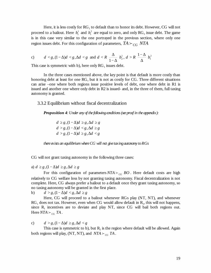
Here, it is less costly for RG1 to default than to honor its debt. However, CG will not proceed to a bailout. Here 1
1b and 21b are equal to zero, and only RG2 issue debt. The game
is in this case very similar to the one portrayed in the previous section, where only one region issues debt. For this configuration of parameters, NTATA CGf
c) γδγδγδ <∆<∆−< ,)1(, and 121
bR
∆−∆<δ , 2
11
bR
∆∆−>δ
This case is symmetric with b), here only RG1 issues debt.
In the three cases mentioned above, the key point is that default is more costly than honoring debt at least for one RG, but it is not as costly for CG. Three different situations can arise –one where both regions issue positive levels of debt, one where debt in R1 is issued and another one where only debt in R2 is issued- and, in the three of them, full taxing autonomy is granted.
3.3.2 Equilibrium without fiscal decentralization
Proposition 4: Under any of the following conditions (see proof in the appendix): γδγδγδ ≥∆≥∆−≥ ,)1(, γδγδγδ ≥∆<∆−> ,)1(,
γδγδγδ <∆≥∆−> ,)1(, there exists an equilibrium where CG will not give taxing autonomy to RGs
CG will not grant taxing autonomy in the following three cases: a) γδγδγδ ≥∆≥∆−≥ ,)1(,
For this configuration of parameters BONTA CGf . Here default costs are high relatively to CG welfare loss by not granting taxing autonomy. Fiscal decentralization is not complete. Here, CG always prefer a bailout to a default once they grant taxing autonomy, so no taxing autonomy will be granted in the first place. b) γδγδγδ ≥∆<∆−> ,)1(,
Here, CG will proceed to a bailout whenever RGs play (NT, NT), and whenever RG1 does not tax. However, even when CG would allow default in R1, this will not happens, since R1 incentives are to deviate and play NT, since CG will bail both regions out. Here TANTA CGf . c) γδγδγδ <∆≥∆−> ,)1(,
This case is symmetric to b), but R2 is the region where default will be allowed. Again both regions will play, (NT, NT), and TANTA CGf .
20
One of the interesting points in cases b) and c) is that while in each of the cases there are incentives for one region to tax, knowing that a bailout is feasible in the event of the other region default, the region where default will be allowed ends up being bailed out as well.
4. An application to Argentina and some policy implications The case of Argentina is just an example which can be extended to all Eastern
European countries intending to join the Euro since; any country joining a monetary union will have consequences for its fiscal sector. Giving up monetary policy limits the amount of tools available to finance government -both central and regional- deficits. Also, the model can be applied to the CFA zone in Africa, where there has been Convertibility to the Franc -now the Euro- for more than thirty years. Finally, we can apply the model to Ecuador, where the economy is dollarized since 2000. In what follows we will take a close look to the Argentine case, since the country underwent a process of giving up its monetary authority. While it achieved a significant reduction in inflation, it was not able to achieve fiscal discipline (at least at the sub-national level). This indiscipline caused great indebtedness and forced the central government to abandon the peg and to default on its debt.
This section rests heavily on Saiegh and Tommasi (1999)16 and tries to summarize briefly some of the main problems of Argentina’s tax sharing regime. The two main problems are the lack of fiscal correspondence between sub-national revenues and expenditures and the central government recurrent bailouts of sub-national units.
First of all, there is a lack of fiscal correspondence, with very little tax effort on behalf of the provinces and a large proportion of services provided by them. Second, the bailout problem, where CG generally bails out lower levels of government, creates a moral hazard problem.
Argentina is a federal country17, where the regional governments (provinces) have a great deal of autonomy. Expenditures are highly decentralized and provinces have borrowing autonomy. However, taxes are still heavily centralized at the national government. Taxes are collected by the Central Government (CG) and then re-distributed in the form of transfers to the provinces (RG) though a system called “Coparticipacion Federal” (tax-sharing agreement). Provinces differ in both share of the national income and in population. The tax-sharing agreement as it is today presents two main problems:
1. The unit of redistribution of CG revenues is the region and not the households. This has been historically the case since governors of the different regions give their support to the CG. The power of each governor in the Upper house of the Congress does not bear any relationship with the population or share of income of the different regions. So bigger regions are under-represented and smaller regions are over-represented. So, per capita transfers differ widely across regions.18
16 Saiegh, Sebastian M, Tommasi, Mariano (1999) 17 This is just a brief summary of the main pillars of Argentina fiscal structure. A much more detailed description can be found in Piffano (1998), Tommasi, Sanguinetti and Saiegh (2001). 18 It is the case for example, that poor living in richer and highly densely populated provinces receive much lower transfers per capita than poor living in poorer and low density populated provinces.

21
2. The second problem is derived directly from the first one, and it is the deficit bias that this way of sharing transfers creates. For bigger and wealthier provinces (wealthier in terms of higher share of income, not in terms of per capita income), the incentive to run deficits is too big. They create most of the taxable income of the country and they are not able to reap its benefits. Poorer regions do not have any incentives to reduce their deficits either. In this case, any fiscally responsible region will receive fewer transfers than its fiscally irresponsible neighbor. But, regardless of the wealth or the regions, there is a lack of fiscal correspondence between the benefit of enjoying public goods and the cost to provide them. Moreover, the fact that RGs have borrowing autonomy makes matters even worse, since many provinces generally run large deficits, borrow abroad and then wait for the CG to bail them out.
As mentioned before, Argentina historically financed its all level government deficits
mainly by printing money. This mechanism resulted in high and increasing inflation, ending in two hyperinflation episodes in 1989-1990. For example, the “inflation tax” amounted to 11.3% of total revenues in 1983. As the inflationary process accelerated by the late eighties, there was clear political consensus that this way of deficit financing must be ended. In this sense, the currency board eliminated the “inflation tax”, but this mechanism was replaced by issuing debt, guaranteeing regional debt with national revenues or transferences.
In 1991 a currency board called “Convertibility regime” 19 was established. The main objective of this exchange rate regime was to reduce inflation. The peg, however, implied some well known policy trade-offs. Among many others, this exchange rate regime prevents the government from printing money to finance its deficits. In this sense, one of the results of adopting a currency board is that it acted as implicit hardening of the budget constraint. Given the structure of all level governments in Argentina, Convertibility meant that the CG should introduce reforms in the tax system and in government expenditures. The CG moved quickly in terms of expenditure decentralization but faced harder challenges when attempted tax reforms. Sub-national governments cannot cover their expenditures with local taxes and they must be financed by the CG by means of transfers or borrowing. This problem is known as vertical imbalance.(See Table 1) Table 1 Argentina Brazil Chile Mexico Latin American (average) Decentralization (1) (%) 49.3 45.6 13.6 25.4 14.6 Vertical Fiscal imbalance (2) (%)
56.0 33.0 61.0 61.0 52.0
Borrowing autonomy(3) 3.0 2.9 0.0 1.8 n/a (1): the ratio of sub-national/total government spending, (2): the ratio of intergovernmental (sub-national) /total revenue, (3): the value of the index ranks from zero (no borrowing autonomy) to a maximum of four points. Source: Inter-American Development Bank, Fiscal Stability with Democracy and Decentralization, 1997.
19 The “Convertibility Law” was the cornerstone of a stabilization program. A currency board that lasted for 10 years was established, where one peso (Argentine currency unit) was equal to one USD. The peg was abandoned in January 2002. To see an account of the problems that led to the currency crisis see Galiani, Heymann and Tommasi (2002).

22
In terms of our model’s assumption, we have to make some comments in order to
make it consistent with the argentine example. The population weights ∆ and )1( ∆− in CG’s welfare function are not representative for Argentina, due to the fact that for political reasons CG redistributes resources across regions for other factors than population Moreover, CG often needs governors’ support in Congress, so in terms of transferences to the provinces it is often the case that per capita transfers are higher in low densely populated provinces. Currently, the tax sharing regime is based on the following weights, 65% on population, 10% according to demographic dispersion and 25% according to the development gap, defined as the difference between each province wealth with respect to the richest one.
With regards to the parameter γ, we can mention one interesting example of this extra effort on behalf of the CG when collecting revenues was the privatization of the Social Security System in 1994. Abandoning the state-funded PAYG system reduced the amount of instruments in the hands of the CG in order to bailout regions, so it has to resort to borrowing, which resulted in an accumulation of an unsustainable level of debt.
As regards to CG transferences to RGs, past expenditure decentralization in Argentina has been an attempt to begin to improve the problem of resource allocation from the point of view of expenditures. But the main drawback of such process has been the impossibility of achieving some degree of tax decentralization. The Central Government has lost control over expenditure decisions –making any adjustment more difficult- but it must raise revenues in order to finance sub-national expenditures. The transfers to sub-national governments are automatically guaranteed by the Tax Sharing Agreement, which poses a burden on Central Government accounts. Any economic downturn complicates the fiscal solvency of the Central Government, since it has to provide funds to the regional units with little flexibility in expenditure20.
As far as bailouts from CG are concerned, as Nicolini et. al (2002) conclude, there were
“several episodes of bailout in the relationship between provinces and the national government. The main features of those episodes were
20 As we can see from the table below, transfers as a % of current expenditures have been increasing in past years.
1993 34,6%
1994 33,3%
1995 29,5%
1996 30,8%
1997 30,6%
1998 30,9%
1999 40,6%
2000 40,0%
2001 38,0%
2002 43,7%
2003 47,1%
2004 (1st. Qr) 49,4%
Source: IERAL based on MECON
Transfers to the provinces as % of CG Current Expenditures

23
associated with jurisdictions running very unsustainable fiscal policies that at some point moved the province into almost bankruptcy.”21
Finally, it is worth mentioning the last episode of CG bailout. Before the abandoning
of the Convertibility, the RG have issued “monies”22 worth $6 billion23. In 2002-2003 the CG bailed out the provinces by absorbing their debt once again.
At this point, we can mention some policy implications we can draw directly from
the model we presented that would help to achieve complete fiscal decentralization. Among them we can mention: limits to regional debt, structure of debt return and default costs.
If issuing debt is not allowed for RGs, then the problem disappears. But this solution is a bit hard to implement in a context of federal countries. Also, debt allows regions to achieve intertemporal efficiency in consumption, which will not happen is the regions are forced not to issue debt. Some countries (Switzerland and Norway for example)24 have limits for their subnational governments as to what they can finance by issuing debt, for example, it is not possible to finance current expenditures. Debt issuing is used instead to finance infrastructure projects, where the benefits are enjoyed and paid not only by the current but by future generations.
If the structure of returns on debt are made state contingent, i.e. α in our previous model is sufficiently low for the bad state of nature increases the probability that RG will choose regional taxation. In this sense, recent Argentine national debt that pays a premium for higher GDP growth can be an example. But there are no cases so far for subnational government debt.
Increasing default costs have two opposite effects. On one hand, it reduces the attractiveness of RG’s default with respect to the costs of regional taxation. But, on the other hand, it increases CG incentives for a bailout in the first place, unless the region we are considering is sufficiently small.
Finally, we would like to stress that there is nothing in dollarization which eliminates RG’s incentives to overspend, given the possibility of a CG bailout. This mechanism penalizes fiscally prudent regions, which end up bearing part of the cost of repaying other regions debt.
5. Conclusions
The advocacy towards fiscal decentralization both in the provision of public goods
and in revenue collection is a popular policy recommendation across international institutions. Many developing countries and transition economies are engaged in such processes, but so far and to different extents, some countries have failed in achieving an optimum level of fiscal decentralization in terms of Oates’ theorem.
It is often the case that some central governments find it very difficult to discipline sub-national governments and thus, implementing complete fiscal decentralization may not
21 A listing of CG bailout episodes can be found in Nicolini et al. (2002) 22 Many provinces issued small denomination bonds that looked very similar to a note. 23 M1 at that time was around $ 42 billions. 24 A good account of the different debt restrictions for sub national governments in different countries can be found at http://www.decentralization.org

24
happen. We developed two very simple models in a game theoretic framework to analyze interactions between a regional government and a central government and then regions interacting with the central government. Our results suggest that according to different parameters configurations we can obtain two sets of equilibria, one where complete fiscal decentralization is achieved and a second one, where it is not. Contrary to our priors, endowment volatility played no role on central government beliefs.
For the first model, where only one region is active, the model can be understood as follows: the central government (CG) is a mechanism used by the provinces to pass to each other tax pressure to finance their expenditure levels, here, only from R1 to R2. In this sense, it can be compared to a model with externalities, pollution externalities, for example, in which there is a higher than optimal level of pollution. This can be solved either with a central planner or privatizing the cost and benefits of fiscal decisions. For the case of the paper, the solution is either centralizing back all regional expenditures. The only difference with typical externality models is the existence of risk, i.e. the possibility of an adverse shock in the second period. As we have shown, output volatility plays no role in the sense that CG actions are independent of the realization of endowments. It matters just for RG’s decision whether to tax its citizens or allowing default. Given this externality, there is a higher level of regional debt, and hence, increasing the probability of a fiscal crisis.
The different sets of equilibria obtained will have different welfare implications for the individuals in each region. The equilibrium with regional taxation is preferred by individuals in region 2, while individuals in region 1 prefer to be bailed out by the Central Government. As it was mentioned before there are different parameters configurations that matters for the choice of equilibrium. The first of them is regional size, since the Central Government weights each region according to its population. The bigger region 1 is, the lower the range of parameters for which the Central Government will give taxing autonomy. Secondly, endowment volatility will also matter. Higher endowment volatility also reduces the scope for granting taxing autonomy for regional governments. Finally, debt holding distributions also should be taken into account. Any legal limitation to the holding of debt outside the region or debt caps to regional debt will also work in this direction.
When we allow for regional interaction, our results do not change significantly. There are still different parameter configurations which sustain an equilibrium with decentralization and another one without it. The interesting addition is that even in the case where the central government will allow default for one specific region, such region has an incentive to deviate from taxing, since the central government will proceed to a bailout if both regions default.
We also looked at adopting “dollarization” -or any equivalent hard monetary rule where the government has no control over monetary policy- as a commitment technology to induce fiscal discipline in sub-national governments and found that there is nothing about dollarization that aims at eliminating this mechanism. The only thing that is different is the way of “taxing” the externality we mention above.
Among the many extensions which can be considered, we will mention some for future work. The assumption that R is exogenous can be too strong, since regional debt returns play a role in deficit sustainability in most federal countries. Also, default costs are set to be fixed and exogenous. The game can be extended to a multiregional context, and with different specification of welfare functions for the Central Government. As far as the sequence of the game is stated, we made no comment as to why CG starts by decentralizing expenditures first; we model it in that way since it is the most common trend observed in

25
practice. Probably, it is due to political reasons that decentralization evolves in this way. Here we take the sequence as given.
Also, the model can be modified to allow for monetary policy aiming at studying welfare implications of a central government bailout by means of an inflation tax. In the models we have presented, there is no difference between a nation-wide tax and the inflation tax, but the model can become more sophisticated by allowing some regional or agent heterogeneity with different welfare effects between the two options for bailout.
Finally, while default never arises in equilibrium, we do observe defaults of regional and central governments in practice. But this is a common feature of a great bulk of literature concerned with default.
The goal of this paper was to twofold. First, we wanted to see if it was theoretically plausible to obtain economies that get “stuck” in the middle of a process of incomplete fiscal decentralization. Here, the problem of vertical imbalance continues, and regional deficits and regional debt is too high. Secondly, we wanted to check whether dollarization or hard pegs are successful in inducing fiscal discipline. In this sense, we observe that central government bailouts do not disappear. While in Cooper et. al (2003) bailout takes the form of monetization of regional deficits, dollarization does not rule out bailouts totally, since a Central Government tax bailout is always possible. The model can be applied to economies like Argentina, Ecuador and African countries in the CFA zone.

26
References [1] Alzua, M.L. “Optimal debt Management: the case for Venezuela”, working paper,
May 2002
[2] Cooper, Russell, Kempf, Hubert, “Designing Stabilization Policy in a Monetary
Union”, NBER Working Paper 7607, March 2000.
[3] Cooper, Russell, Kempf, Hubert and Peled, Dan. “Is it is or is it Ain't my
Obligation? Regional Debt in Monetary Unions”, NBER Working Paper 10239,
January 2004
[4] Cooper, Russell and Hubert Kempf. “Dollarization and the Conquest of
Hyperinflation in Divided Societies”, Federal Reserve Bank of Minneapolis Quarterly
Review, 25 (3).
[5] Freire, Maria E., Marcela Huertas and Benjamin Darche. “Sub-national Access to
Capital Markets: the Latin American Experience”, unpublished, the World Bank,
1998.
[6] Galiani, Sebastian, Daniel Heymann and Mariano Tommasi ,”Great Expectations
and Hard Times: The Argentine convertibility plan”, Economia, Journal of the Latin
American and Caribbean Economic Association, Vol 3 (2), 2003, pp. 109-160
[7] Garcia Mila, Teresa and Therese McGuire, “Do Interregional Transfers Improve the
Economic Performance of Poor Regions? The Case of Spain”, mimeo, December,
1996.
[8] Giugale, Marcelo, Adam Korobow and Steven Webb, “A New Model for Market-
based Regulation of Sub-national borrowing: The Mexican Approach”, mimeo,
World Bank
[9] Gonzalez, Christian, David Rosenblatt and Steven Webb, “Stabilizing
Intergovernmental Transfers in Latina America: A Complement to
National/Subnational Fiscal Rules?”, World Bank Policy Research Working Paper
2869, July 2002
[10] Krugman, Paul, “A Model of Balance of Payments Crises”, Journal of Money,
Credit and Banking, Vol , No. 3 (August 1979), 311-325

27
[11] Oates, Wallace, “An Essay on Fiscal Federalism”, JEL, Vol XXXVII (September
1999), pp 1120-1149
[12] Person, Torsten and Guido Tabellini, “Political Economics: Explaining Economic
Policy”, MIT Press, 2000.
[13] Sturzenegger, Federico and Mariano Tommasi, “The Political Economy of
Reform”, MIT Press, 1998.
[14] Tommasi, Mariano, “Federalism in Argentina and the Reforms of the1990’s”,
Working Paper 147, Center for Research on Economic Development and Policy
Reform, Stanford University, August 2002.
[15] Tommasi, Mariano, Sebastian Saiegh and Pablo Sanguinetti, “Fiscal Federalism in
Argentina: Policies, Politics and Institutional Reform”, Revista Economia, Spring
2001
[16] Shah, Anwar, “Fiscal Federalism and Macroeconomic Governance: For Better or for
Worse?”, mimeo, World Bank, June 1997

28
Appendix 1: Game with no regional interaction Game: Figure 1
p (1-p)
Yhigh Ylow
CG Taxing Authority
No Taxing Authority
Taxing Authority
No Taxing Authority
RG Tax (1) No Tax Bailout1 (4) Tax (5) No Tax Bailout1 (8)
CG Bailout2 (2) Default (3) Bailout2 (6) Default (7)
The joint strategies of both players are:
=Γ=Γ ),( RGCG {[(TA, BO2), (Tax,Tax)], [(TA, BO2), (Tax,No Tax)], [(TA, BO2), (No
Tax,Tax)], [(TA, BO2), (No Tax,No Tax)], [(TA, D), (Tax,Tax)], [(TA, D), (Tax,No Tax)],
[(TA, D), (No Tax,Tax)], [(TA, D), (No Tax,No Tax)], [NTA(BO1), -i]}, where i is any
action taken by RG1.
We construct the pay-offs for each node of the game:
(1) hCG yW +Π=
21bRyW hhRG
∆∆−−=
(2) hCG yW +−Π= γ

29
21bRAyW hhRG
∆∆−−= , where
∆∆−+∆= )1(τ
A
(3) hCG yW +∆−Π= δ
δ−= hRG yW
(4) hCG yW +Π=
21bRAyW hhRG
∆∆−−=
(5) lCG yW +Π=
21 bRyW hlRG α
∆∆−−=
(6) lCG yW +−Π= γ , where
21bRAyW hlRG α
∆∆−−=
(7) lCG yW +∆−Π= δ
δ−= lRG yW
(8) lCG yW +Π=
21bRAyW hlRG α
∆∆−−=
Equilibria
In order to define a Weak Perfect Bayesian Equilibrium we must define a set of strategies and system of beliefs ( )µσ, such that σ is sequentially rational given the system of beliefs µ and the system of beliefs µ is derived from strategy profile σ through Bayes’ rule whenever possible.

30
Last stage of the game
CG will prefer Bailout2 to default for the following set of beliefs:
≥−+Π−+−+Π↔ ))(1()(2 γµγµ lhCG yyDBO f
))(1()( δµδµ ∆−+Π−+∆−+Π≥ lh yy , which requires δγ ∆< with no restrictions on
CG’s beliefs.
If δγ ∆< , there are no restrictions on beliefs, and CG will always prefer to bail out the regions than to allow default. As γincreases, a bailout becomes more costly in terms of CG welfare. This also will depend of the size of R1 and the technology that penalizes default. Note than here, increasing default costs, increases the set of values of γfor which CG will prefer a bailout. Also, there are no restrictions on beliefs µ , so output volatility does not matter in order for the CG to choose a course of action.
Second stage of the game
RG1 has the following strategies for each realization of endowment: (Tax, Tax), (Tax, No
Tax), (No Tax, No Tax), (No Tax, Tax)
a) δγ ∆< DBO CGf2⇔
a.1. Left node: TaxTaxNo RGf , whenever ( ) 01 ≥∆−τ , which is always the case.
RG will always choose no regional taxation.
a.2 Right node: TaxTaxNo RGf , whenever ( ) 01 ≥∆−τ , which is always the case.
RG will always choose no regional taxation as in the left node. Here again, output volatility
plays no role in the set of strategies that is chosen.
Whenever RG1 knows CG will proceed to a bailout, then, they will never choose
taxation, since by a bailout RG can pass the cost of repaying RG1 debt to R2 individuals.
This means higher consumption for R2 agents in the second period.
b) δγ ∆< 2BOD CGf⇔
b.1. Left node: TaxTaxNo RGf , whenever 21bRh
∆∆−≤δ (*)

31
b.2 Right node: TaxTaxNo RGf , satisfied whenever 21bRhαδ
∆∆−≤ .(**)
Default costs δwhich satisfy (**), will also satisfy 21bRh
∆∆−≤δ , since 1<α . If, (*) holds
but (**) does not, then RG will choose taxation in the bad realization of endowment but no taxation when endowments are high. This seems a little counterintuitive, since one would expect that the lower realization of output would induce the RG to be more inclined towards a bailout. This depends on α . When α small, then the tax effort in terms of output is is low, so consumption will increase with regional taxation relative to default. By increasing default costs, the set for which (*) holds is reduced, but the probability of a CG bailout increases. Unless the loss in welfare for CG γis too high, then increasing default costs has this potential harmful effect in terms of regional taxation. First stage
a) DBO CGf2⇔∆≤ δγ and TaxTaxNo RGf (under 0)1( ≥∆−τ ) ⇔TANTA CGf , is always preferred regardless of p. Here, output volatility plays no role in
deciding whether CG will give taxing autonomy or not. Given that CG will bailout RG, then it prefers not to grant TA in the first place, increasing CG welfare by γ.
b) 2BOD CGf⇔∆> δγ and TaxTaxNo RGf (under (*) and (**)
TANTA CGf , always.

32
Appendix 2: Game with regional interaction
CGGame: Figure 2
CG
Taxing Authonomy No Taxing Authonomy (8)
RG1T NT
RG2 T (1) NT T NT
CG Bailout2 (2) Default (3) Bailout2 (4) Default (5) Bailout2 (6) Default (7)
The joint strategies of the three players are: G = G(CG, RG1, RG2) ={[(TA, BO), (T), (T)], [(TA, BO), (T), (NT)], [(TA, BO), (NT), (T)], [(TA, BO), (NT), (NT)], [(TA, D), (T), (T)], [(TA, D), (T), (NT)], [(TA, D), (NT), (T)], [(TA, D), (NT), (NT)], (TA, BO), (-i), (-j)], where i and j are any action taken by RG1 and RG2 respectively.
We construct the pay-offs for each node of the game:
(1) yW CG +Π=
21
121
11 RbRbycW oRG
∆∆−−+==
12
212 1
2 RbRbycW oRG
∆−∆−+==
(2) δ)1( ∆−−+Π= yW CG
211
11 RbycW oRG
∆∆−−==
δ−+== 212
2 RbycW oRG

33
(3) γ−+Π= yW CG
[ ] 21
22
121
1)1(1 RbRbRbycW oRG
∆∆−−−∆−+==
21
12
222 )(2 RbRbRbycW oRG +−∆+==
(4) δ∆−+Π= yW CG
δ−+== 121
1 RbycW oRG
122 1
2 RbycW oRG
∆−∆+==
(5) γ−+Π= yW CG
[ ] 12
21
111 )1(1 RbRbRbycW oRG +−∆−+==
[ ] 12
11
212 1
2 RbRbRbycW oRG
∆−∆−−∆+==
(6) δ−+Π= yW CG
δ−== ycW oRG1
1
δ−== ycW oRG2
2
(7) γ−+Π= yW CG
ycW oRG == 11
ycW oRG == 22
(8) yW CG +Π=
ycW oRG == 11
ycW oRG == 22
Equilibria
In order to define a Sub-game Perfect Nash Equilibrium we must define a set of strategies G such G constitutes a Nash Equilibrium in every sub-game.

34
Last stage of the game
CG will prefer Bailout2 to default for the following configuration of parameters:
I) δγ )1( ∆−−+Π≥−+Π↔ yyDBO CGf
γδ≥∆− )1(
II) δγ ∆−+Π≥−+Π↔ yyDBO CGf
γδ≥∆
III) δγ −+Π≥−+Π↔ yyDBO CGf
γδ≥
If I) and II) are satisfied BO dominates D, III) will be satisfied too.
Second stage of the game Cases:
I) DBO CGf⇒≥∆≥∆−≥ γδγδγδ ,)1(,
II) BOD CGf⇒<∆<∆−< γδγδγδ ,)1(,
III) DBO CGf⇒> γδ
BOD CGf⇒<∆− γδ)1(
DBO CGf⇒≥∆ γδ
IV) DBO CGf⇒δγ
DBO CGf⇒>∆− γδ)1(
BOD CGf⇒<∆ γδ

35
RG1 and RG2 play the following simultaneous move game: I) DBO CGf⇒≥∆≥∆−≥ γδγδγδ ,)1(,
R2 T NT
R1
T
21
12
01
1bRRbyc
∆∆−−+=
12
21
02 1
bRRbyc
∆−∆−+=
∆−+
∆∆−−∆−+= 2
221
12
01 )1(
1)1( bbRRbyc
12
21
22
02 bRRbRbyc ∆−+∆+=
NT
∆+
∆−∆−∆+= 1
112
21
01 1
bbRRbyc
12
21
02 1
bRRbyc
∆−∆−+=
yc =01
yc =02
NE: (NT, NT) II) BOD CGf⇒<∆<∆−< γδγδγδ ,)1(,
R2 T NT
R1
T
21
12
01
1bRRbyc
∆∆−−+=
12
21
02 1
bRRbyc
∆−∆−+=
21
01
1bRyc
∆∆−−=
δ−+= 21
02 Rbyc
NT
δ−+= 12
01 Rbyc
12
02 1
bRyc
∆−∆−=
δ−= yc01
δ−= yc02
NE: It depends on the parameters, there can be 4 equilibria:
(NT, NT), whenever 21
1bR
∆∆−<δ , 1
21bR
∆−∆<δ , autarky, no debt holdings.
(NT, T), whenever <
∆∆− 2
11
bR 121
bR
∆−∆<δ , only R1 issues debt.
(T, NT), whenever <
∆∆− 1
21
bR 121
bR
∆−∆<δ , only R2 issues debt.

36
(T, T), whenever 21
1bR
∆∆−<δ , 1
21bR
∆−∆<δ , whenever default cost are high, and
increase in default costs increases the set of parameters for which (T,T) is sustained) III) DBO CGf⇒> γδ (NT, NT)
BOD CGf⇒<∆− γδ)1( (T, NT) DBO CGf⇒≥∆ γδ (NT, T)
R2 T NT
R1
T
21
12
01
1bRRbyc
∆∆−−+=
12
21
02 1
bRRbyc
∆−∆−+=
21
01
1byc
∆∆−−=
δ−+= 21
02 Rbyc
NT
12
21
11
01 ))(1( RbbbRyc +−∆−+=
12
11
21
02 1
)( bRbbRyc
∆−∆−−∆+=
yc =01
yc =02
NE: (NT, NT) IV) DBO CGf⇒> γδ (NT, NT)
DBO CGf⇒>∆− γδ)1( (T, NT)
BOD CGf⇒<∆ γδ (NT, T)
R2 T NT
R1
T
21
12
01
1bRRbyc
∆∆−−+=
12
21
02 1
bRRbyc
∆−∆−+=
21
22
12
01
1))(1( bbbyc
∆∆−−−∆−+=
21
12
22
02 )( Rbbbyc +−∆+=
NT
δ−+= 12
01 Rbyc
12
02 1
bRyc
∆−∆−=
yc =01
yc =02
NE: (NT, NT) First stage
37
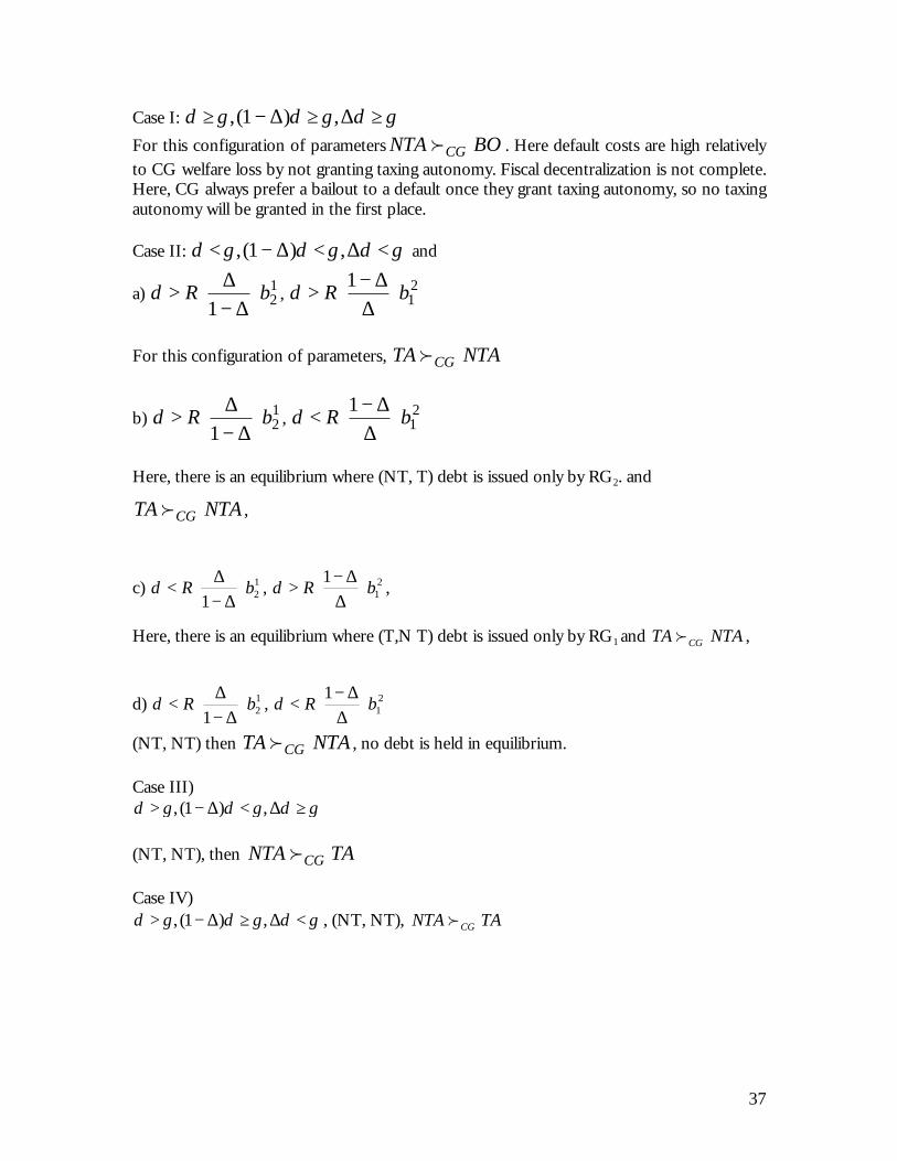
Case I: γδγδγδ ≥∆≥∆−≥ ,)1(,
For this configuration of parameters BONTA CGf . Here default costs are high relatively to CG welfare loss by not granting taxing autonomy. Fiscal decentralization is not complete. Here, CG always prefer a bailout to a default once they grant taxing autonomy, so no taxing autonomy will be granted in the first place. Case II: γδγδγδ <∆<∆−< ,)1(, and
a) 121
bR
∆−∆>δ , 2
11 bR
∆∆−>δ
For this configuration of parameters, NTATA CGf
b) 121
bR
∆−∆>δ , 2
11 bR
∆∆−<δ
Here, there is an equilibrium where (NT, T) debt is issued only by RG2. and
NTATA CGf ,
c) 121
bR
∆−∆<δ , 2
11
bR
∆∆−>δ ,
Here, there is an equilibrium where (T,N T) debt is issued only by RG1 and NTATA CGf ,
d) 121
bR
∆−∆<δ , 2
11
bR
∆∆−<δ
(NT, NT) then NTATA CGf , no debt is held in equilibrium. Case III)
γδγδγδ ≥∆<∆−> ,)1(, (NT, NT), then TANTA CGf Case IV)
γδγδγδ <∆≥∆−> ,)1(, , (NT, NT), TANTA CGf