Efficiently finding optimal winding-constrained loops in the planePaul Vernaza, Venkatraman Narayanan, and Maxim Likhachev

pvernaza@cs.cmu.edu, venkatrn@andrew.cmu.edu, maxim@cs.cmu.edu

The Robotics InstituteCarnegie Mellon University

Pittsburgh, PA 19104

Abstract—We present a method to efficiently find winding-constrained loops in the plane that are optimal with respectto a minimum-cost objective and in the presence of obstacles.Our approach is similar to a typical graph-based search for anoptimal path in the plane, but with an additional state variablethat encodes information about path homotopy. Upon finding aloop, the value of this state corresponds to a line integral overthe loop that indicates how many times it winds around eachobstacle, enabling us to reduce the problem of finding pathssatisfying winding constraints to that of searching for paths tosuitable states in this augmented state space. We give an intuitiveinterpretation of the method based on fluid mechanics and showhow this yields a way to perform the necessary calculationsefficiently. Results are given in which we use our method tofind optimal routes for autonomous surveillance and intrudercontainment.

I. INTRODUCTION

The subject of this work is finding optimal constrained loopsin the plane. More specifically, out of all paths starting andending at a specific location in the plane and satisfying certainwinding constraints, we would like to find one such path thatminimizes a given location-dependent cost accumulated alongthe path, while also avoiding some regions entirely.

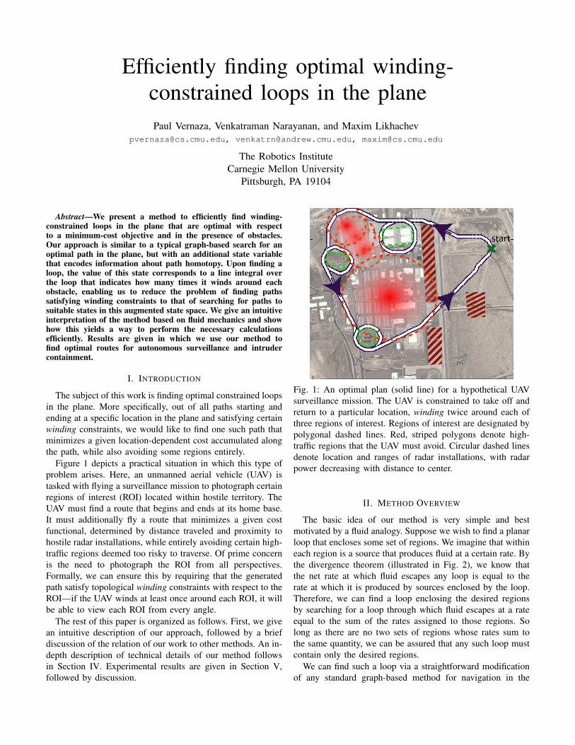
Figure 1 depicts a practical situation in which this type ofproblem arises. Here, an unmanned aerial vehicle (UAV) istasked with flying a surveillance mission to photograph certainregions of interest (ROI) located within hostile territory. TheUAV must find a route that begins and ends at its home base.It must additionally fly a route that minimizes a given costfunctional, determined by distance traveled and proximity tohostile radar installations, while entirely avoiding certain high-traffic regions deemed too risky to traverse. Of prime concernis the need to photograph the ROI from all perspectives.Formally, we can ensure this by requiring that the generatedpath satisfy topological winding constraints with respect to theROI—if the UAV winds at least once around each ROI, it willbe able to view each ROI from every angle.

The rest of this paper is organized as follows. First, we givean intuitive description of our approach, followed by a briefdiscussion of the relation of our work to other methods. An in-depth description of technical details of our method followsin Section IV. Experimental results are given in Section V,followed by discussion.

Fig. 1: An optimal plan (solid line) for a hypothetical UAVsurveillance mission. The UAV is constrained to take off andreturn to a particular location, winding twice around each ofthree regions of interest. Regions of interest are designated bypolygonal dashed lines. Red, striped polygons denote high-traffic regions that the UAV must avoid. Circular dashed linesdenote location and ranges of radar installations, with radarpower decreasing with distance to center.

II. METHOD OVERVIEW

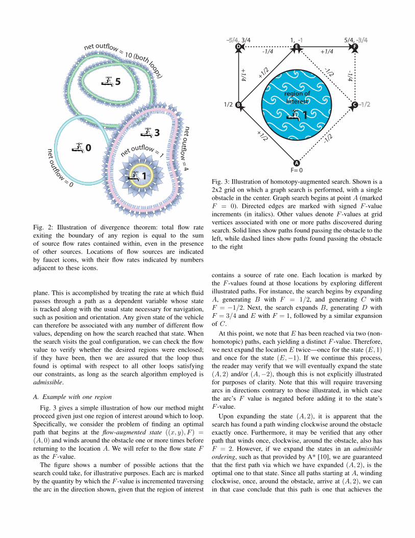
The basic idea of our method is very simple and bestmotivated by a fluid analogy. Suppose we wish to find a planarloop that encloses some set of regions. We imagine that withineach region is a source that produces fluid at a certain rate. Bythe divergence theorem (illustrated in Fig. 2), we know thatthe net rate at which fluid escapes any loop is equal to therate at which it is produced by sources enclosed by the loop.Therefore, we can find a loop enclosing the desired regionsby searching for a loop through which fluid escapes at a rateequal to the sum of the rates assigned to those regions. Solong as there are no two sets of regions whose rates sum tothe same quantity, we can be assured that any such loop mustcontain only the desired regions.

We can find such a loop via a straightforward modificationof any standard graph-based method for navigation in the

1

30

5

net out�ow

= 4

net out�ow = 0

net out�ow = 1

net out�ow = 10 (both loops)

Fig. 2: Illustration of divergence theorem: total flow rateexiting the boundary of any region is equal to the sumof source flow rates contained within, even in the presenceof other sources. Locations of flow sources are indicatedby faucet icons, with their flow rates indicated by numbersadjacent to these icons.

plane. This is accomplished by treating the rate at which fluidpasses through a path as a dependent variable whose stateis tracked along with the usual state necessary for navigation,such as position and orientation. Any given state of the vehiclecan therefore be associated with any number of different flowvalues, depending on how the search reached that state. Whenthe search visits the goal configuration, we can check the flowvalue to verify whether the desired regions were enclosed;if they have been, then we are assured that the loop thusfound is optimal with respect to all other loops satisfyingour constraints, as long as the search algorithm employed isadmissible.

A. Example with one region

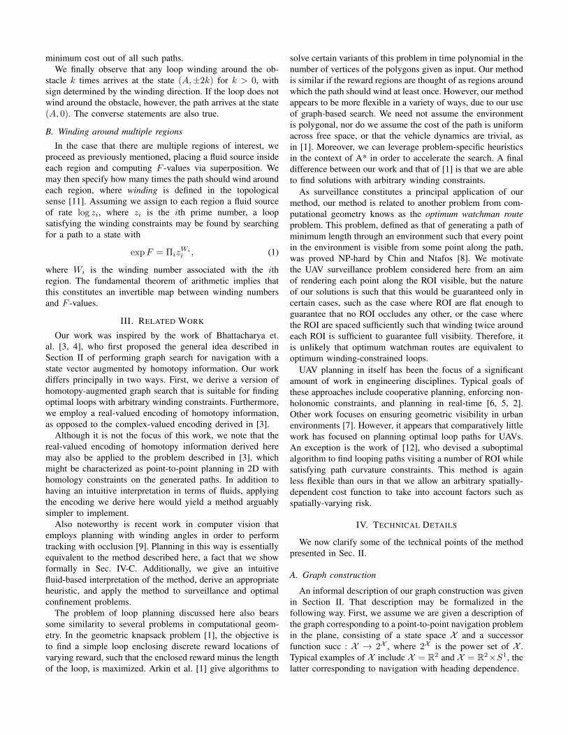
Fig. 3 gives a simple illustration of how our method mightproceed given just one region of interest around which to loop.Specifically, we consider the problem of finding an optimalpath that begins at the flow-augmented state ((x, y), F ) =(A, 0) and winds around the obstacle one or more times beforereturning to the location A. We will refer to the flow state Fas the F -value.

The figure shows a number of possible actions that thesearch could take, for illustrative purposes. Each arc is markedby the quantity by which the F -value is incremented traversingthe arc in the direction shown, given that the region of interest

-1/4

+1/4-1/4

+1/2

+1/2-1/2

-1/2

region ofinterest

F= 0

1/2

+1/4

1, 5/4, 3/4

CB

D E F

A

1

Fig. 3: Illustration of homotopy-augmented search. Shown is a2x2 grid on which a graph search is performed, with a singleobstacle in the center. Graph search begins at point A (markedF = 0). Directed edges are marked with signed F -valueincrements (in italics). Other values denote F -values at gridvertices associated with one or more paths discovered duringsearch. Solid lines show paths found passing the obstacle to theleft, while dashed lines show paths found passing the obstacleto the right

contains a source of rate one. Each location is marked bythe F -values found at those locations by exploring differentillustrated paths. For instance, the search begins by expandingA, generating B with F = 1/2, and generating C withF = −1/2. Next, the search expands B, generating D withF = 3/4 and E with F = 1, followed by a similar expansionof C.

At this point, we note that E has been reached via two (non-homotopic) paths, each yielding a distinct F -value. Therefore,we next expand the location E twice—once for the state (E, 1)and once for the state (E,−1). If we continue this process,the reader may verify that we will eventually expand the state(A, 2) and/or (A,−2), though this is not explicitly illustratedfor purposes of clarity. Note that this will require traversingarcs in directions contrary to those illustrated, in which casethe arc’s F value is negated before adding it to the state’sF -value.

Upon expanding the state (A, 2), it is apparent that thesearch has found a path winding clockwise around the obstacleexactly once. Furthermore, it may be verified that any otherpath that winds once, clockwise, around the obstacle, also hasF = 2. However, if we expand the states in an admissibleordering, such as that provided by A* [10], we are guaranteedthat the first path via which we have expanded (A, 2), is theoptimal one to that state. Since all paths starting at A, windingclockwise, once, around the obstacle, arrive at (A, 2), we canin that case conclude that this path is one that achieves the

minimum cost out of all such paths.We finally observe that any loop winding around the ob-

stacle k times arrives at the state (A,±2k) for k > 0, withsign determined by the winding direction. If the loop does notwind around the obstacle, however, the path arrives at the state(A, 0). The converse statements are also true.

B. Winding around multiple regions

In the case that there are multiple regions of interest, weproceed as previously mentioned, placing a fluid source insideeach region and computing F -values via superposition. Wemay then specify how many times the path should wind aroundeach region, where winding is defined in the topologicalsense [11]. Assuming we assign to each region a fluid sourceof rate log zi, where zi is the ith prime number, a loopsatisfying the winding constraints may be found by searchingfor a path to a state with

expF = ΠizWii , (1)

where Wi is the winding number associated with the ithregion. The fundamental theorem of arithmetic implies thatthis constitutes an invertible map between winding numbersand F -values.

III. RELATED WORK

Our work was inspired by the work of Bhattacharya et.al. [3, 4], who first proposed the general idea described inSection II of performing graph search for navigation with astate vector augmented by homotopy information. Our workdiffers principally in two ways. First, we derive a version ofhomotopy-augmented graph search that is suitable for findingoptimal loops with arbitrary winding constraints. Furthermore,we employ a real-valued encoding of homotopy information,as opposed to the complex-valued encoding derived in [3].

Although it is not the focus of this work, we note that thereal-valued encoding of homotopy information derived heremay also be applied to the problem described in [3], whichmight be characterized as point-to-point planning in 2D withhomology constraints on the generated paths. In addition tohaving an intuitive interpretation in terms of fluids, applyingthe encoding we derive here would yield a method arguablysimpler to implement.

Also noteworthy is recent work in computer vision thatemploys planning with winding angles in order to performtracking with occlusion [9]. Planning in this way is essentiallyequivalent to the method described here, a fact that we showformally in Sec. IV-C. Additionally, we give an intuitivefluid-based interpretation of the method, derive an appropriateheuristic, and apply the method to surveillance and optimalconfinement problems.

The problem of loop planning discussed here also bearssome similarity to several problems in computational geom-etry. In the geometric knapsack problem [1], the objective isto find a simple loop enclosing discrete reward locations ofvarying reward, such that the enclosed reward minus the lengthof the loop, is maximized. Arkin et al. [1] give algorithms to

solve certain variants of this problem in time polynomial in thenumber of vertices of the polygons given as input. Our methodis similar if the reward regions are thought of as regions aroundwhich the path should wind at least once. However, our methodappears to be more flexible in a variety of ways, due to our useof graph-based search. We need not assume the environmentis polygonal, nor do we assume the cost of the path is uniformacross free space, or that the vehicle dynamics are trivial, asin [1]. Moreover, we can leverage problem-specific heuristicsin the context of A* in order to accelerate the search. A finaldifference between our work and that of [1] is that we are ableto find solutions with arbitrary winding constraints.

As surveillance constitutes a principal application of ourmethod, our method is related to another problem from com-putational geometry knows as the optimum watchman routeproblem. This problem, defined as that of generating a path ofminimum length through an environment such that every pointin the environment is visible from some point along the path,was proved NP-hard by Chin and Ntafos [8]. We motivatethe UAV surveillance problem considered here from an aimof rendering each point along the ROI visible, but the natureof our solutions is such that this would be guaranteed only incertain cases, such as the case where ROI are flat enough toguarantee that no ROI occludes any other, or the case wherethe ROI are spaced sufficiently such that winding twice aroundeach ROI is sufficient to guarantee full visibiity. Therefore, itis unlikely that optimum watchman routes are equivalent tooptimum winding-constrained loops.

UAV planning in itself has been the focus of a significantamount of work in engineering disciplines. Typical goals ofthese approaches include cooperative planning, enforcing non-holonomic constraints, and planning in real-time [6, 5, 2].Other work focuses on ensuring geometric visibility in urbanenvironments [7]. However, it appears that comparatively littlework has focused on planning optimal loop paths for UAVs.An exception is the work of [12], who devised a suboptimalalgorithm to find looping paths visiting a number of ROI whilesatisfying path curvature constraints. This method is againless flexible than ours in that we allow an arbitrary spatially-dependent cost function to take into account factors such asspatially-varying risk.

IV. TECHNICAL DETAILS

We now clarify some of the technical points of the methodpresented in Sec. II.

A. Graph construction

An informal description of our graph construction was givenin Section II. That description may be formalized in thefollowing way. First, we assume we are given a description ofthe graph corresponding to a point-to-point navigation problemin the plane, consisting of a state space X and a successorfunction succ : X → 2X , where 2X is the power set of X .Typical examples of X include X = R2 and X = R2×S1, thelatter corresponding to navigation with heading dependence.

We then define a new state space X ′ = X×R, with elementsdenoted by (x, f). Let ρ : X × X → (I → R2) denote thefunction that generates the Cartesian path taken from a nodein the original graph to a successor. succ′ is then defined inthe following way:

succ′ : (x, f) 7→ {(x′, f ′) | x′ ∈ succ(x), f ′ = f+F (ρ(x, x′))},

where F : (I → R2) → R is a line integral that will bedefined formally in the next section.

The start state for graph search is defined by (x0, 0), wherex0 is the start state in the pre-augmented graph. The goalstate is defined as (x0,

∑iWi log zi), where Wi is the desired

winding number of the solution path around the ith region.

B. Line integral constructionAspects of the line integral referred to in the last section

are now detailed. First, we note that a suitable flow field isgiven by

V (x) =∑i

ri2π

x− oi‖x− oi‖2

, (2)

where oi ∈ R2 is an arbitrary source location inside the ithregion for which we are given a winding constraint, and ri =log zi is the source rate assigned to the ith source. This maybe established by considering, for example, the case where oiis located at the center of a circle and devising an integrandthat will integrate to ri. Denoting by n̂(s) the normal to x̃ ats, we define

F (x̃) =

∫V (x̃(s)) · n̂(s) ds. (3)

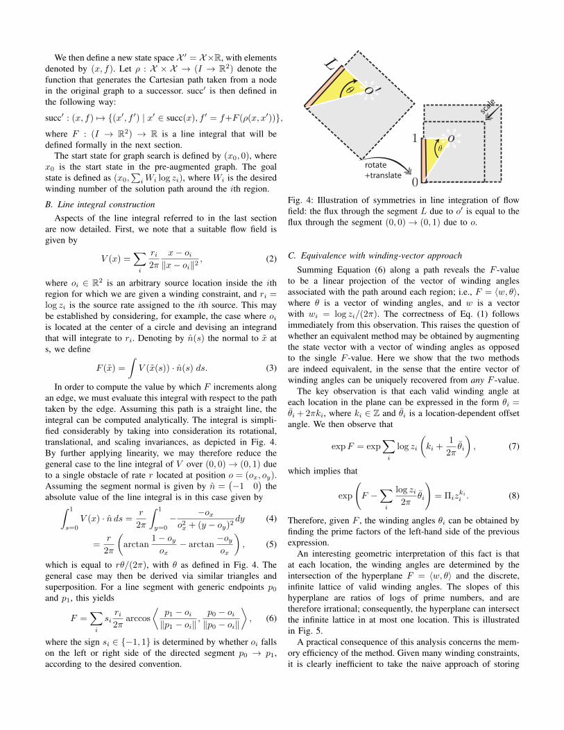
In order to compute the value by which F increments alongan edge, we must evaluate this integral with respect to the pathtaken by the edge. Assuming this path is a straight line, theintegral can be computed analytically. The integral is simpli-fied considerably by taking into consideration its rotational,translational, and scaling invariances, as depicted in Fig. 4.By further applying linearity, we may therefore reduce thegeneral case to the line integral of V over (0, 0)→ (0, 1) dueto a single obstacle of rate r located at position o = (ox, oy).Assuming the segment normal is given by n̂ =

(−1 0

)the

absolute value of the line integral is in this case given by∫ 1

s=0

V (x) · n̂ ds =r

2π

∫ 1

y=0

− −oxo2x + (y − oy)2

dy (4)

=r

2π

(arctan

1− oyox

− arctan−oyox

), (5)

which is equal to rθ/(2π), with θ as defined in Fig. 4. Thegeneral case may then be derived via similar triangles andsuperposition. For a line segment with generic endpoints p0and p1, this yields

F =∑i

siri2π

arccos

⟨p1 − oi‖p1 − oi‖

,p0 − oi‖p0 − oi‖

⟩, (6)

where the sign si ∈ {−1, 1} is determined by whether oi fallson the left or right side of the directed segment p0 → p1,according to the desired convention.

rotate+translate

scale

Fig. 4: Illustration of symmetries in line integration of flowfield: the flux through the segment L due to o′ is equal to theflux through the segment (0, 0)→ (0, 1) due to o.

C. Equivalence with winding-vector approach

Summing Equation (6) along a path reveals the F -valueto be a linear projection of the vector of winding anglesassociated with the path around each region; i.e., F = 〈w, θ〉,where θ is a vector of winding angles, and w is a vectorwith wi = log zi/(2π). The correctness of Eq. (1) followsimmediately from this observation. This raises the question ofwhether an equivalent method may be obtained by augmentingthe state vector with a vector of winding angles as opposedto the single F -value. Here we show that the two methodsare indeed equivalent, in the sense that the entire vector ofwinding angles can be uniquely recovered from any F -value.

The key observation is that each valid winding angle ateach location in the plane can be expressed in the form θi =θ̄i + 2πki, where ki ∈ Z and θ̄i is a location-dependent offsetangle. We then observe that

expF = exp∑i

log zi

(ki +

1

2πθ̄i

), (7)

which implies that

exp

(F −

∑i

log zi2π

θ̄i

)= Πiz

kii . (8)

Therefore, given F , the winding angles θi can be obtained byfinding the prime factors of the left-hand side of the previousexpression.

An interesting geometric interpretation of this fact is thatat each location, the winding angles are determined by theintersection of the hyperplane F = 〈w, θ〉 and the discrete,infinite lattice of valid winding angles. The slopes of thishyperplane are ratios of logs of prime numbers, and aretherefore irrational; consequently, the hyperplane can intersectthe infinite lattice in at most one location. This is illustratedin Fig. 5.

A practical consequence of this analysis concerns the mem-ory efficiency of the method. Given many winding constraints,it is clearly inefficient to take the naive approach of storing

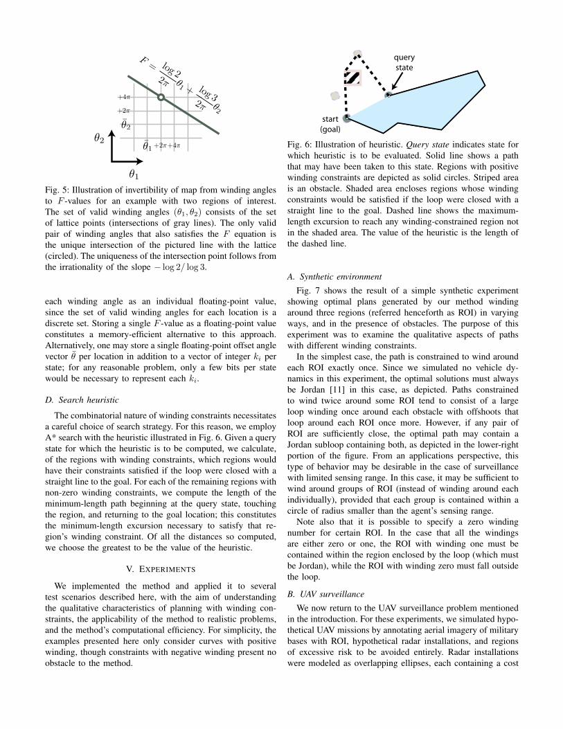
Fig. 5: Illustration of invertibility of map from winding anglesto F -values for an example with two regions of interest.The set of valid winding angles (θ1, θ2) consists of the setof lattice points (intersections of gray lines). The only validpair of winding angles that also satisfies the F equation isthe unique intersection of the pictured line with the lattice(circled). The uniqueness of the intersection point follows fromthe irrationality of the slope − log 2/ log 3.

each winding angle as an individual floating-point value,since the set of valid winding angles for each location is adiscrete set. Storing a single F -value as a floating-point valueconstitutes a memory-efficient alternative to this approach.Alternatively, one may store a single floating-point offset anglevector θ̄ per location in addition to a vector of integer ki perstate; for any reasonable problem, only a few bits per statewould be necessary to represent each ki.

D. Search heuristic

The combinatorial nature of winding constraints necessitatesa careful choice of search strategy. For this reason, we employA* search with the heuristic illustrated in Fig. 6. Given a querystate for which the heuristic is to be computed, we calculate,of the regions with winding constraints, which regions wouldhave their constraints satisfied if the loop were closed with astraight line to the goal. For each of the remaining regions withnon-zero winding constraints, we compute the length of theminimum-length path beginning at the query state, touchingthe region, and returning to the goal location; this constitutesthe minimum-length excursion necessary to satisfy that re-gion’s winding constraint. Of all the distances so computed,we choose the greatest to be the value of the heuristic.

V. EXPERIMENTS

We implemented the method and applied it to severaltest scenarios described here, with the aim of understandingthe qualitative characteristics of planning with winding con-straints, the applicability of the method to realistic problems,and the method’s computational efficiency. For simplicity, theexamples presented here only consider curves with positivewinding, though constraints with negative winding present noobstacle to the method.

start(goal)

querystate

Fig. 6: Illustration of heuristic. Query state indicates state forwhich heuristic is to be evaluated. Solid line shows a paththat may have been taken to this state. Regions with positivewinding constraints are depicted as solid circles. Striped areais an obstacle. Shaded area encloses regions whose windingconstraints would be satisfied if the loop were closed with astraight line to the goal. Dashed line shows the maximum-length excursion to reach any winding-constrained region notin the shaded area. The value of the heuristic is the length ofthe dashed line.

A. Synthetic environment

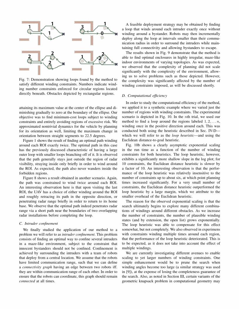
Fig. 7 shows the result of a simple synthetic experimentshowing optimal plans generated by our method windingaround three regions (referred henceforth as ROI) in varyingways, and in the presence of obstacles. The purpose of thisexperiment was to examine the qualitative aspects of pathswith different winding constraints.

In the simplest case, the path is constrained to wind aroundeach ROI exactly once. Since we simulated no vehicle dy-namics in this experiment, the optimal solutions must alwaysbe Jordan [11] in this case, as depicted. Paths constrainedto wind twice around some ROI tend to consist of a largeloop winding once around each obstacle with offshoots thatloop around each ROI once more. However, if any pair ofROI are sufficiently close, the optimal path may contain aJordan subloop containing both, as depicted in the lower-rightportion of the figure. From an applications perspective, thistype of behavior may be desirable in the case of surveillancewith limited sensing range. In this case, it may be sufficient towind around groups of ROI (instead of winding around eachindividually), provided that each group is contained within acircle of radius smaller than the agent’s sensing range.

Note also that it is possible to specify a zero windingnumber for certain ROI. In the case that all the windingsare either zero or one, the ROI with winding one must becontained within the region enclosed by the loop (which mustbe Jordan), while the ROI with winding zero must fall outsidethe loop.

B. UAV surveillance

We now return to the UAV surveillance problem mentionedin the introduction. For these experiments, we simulated hypo-thetical UAV missions by annotating aerial imagery of militarybases with ROI, hypothetical radar installations, and regionsof excessive risk to be avoided entirely. Radar installationswere modeled as overlapping ellipses, each containing a cost

1 1

1

222

3 1

0

1 22

Fig. 7: Demonstration showing loops found by the method tosatisfy different winding constraints. Numbers indicate wind-ing number constraints enforced for circular regions locateddirectly beneath. Obstacles depicted by rectangular regions.

attaining its maximum value at the center of the ellipse and di-minishing gradually to zero at the boundary of the ellipse. Ourobjective was to find minimum-cost loops subject to windingconstraints and entirely avoiding regions of excessive risk. Weapproximated nontrivial dynamics for the vehicle by planningfor its orientation as well, limiting the maximum change inorientation between straight segments to 22.5 degrees.

Figure 1 shows the result of finding an optimal path windingaround each ROI exactly twice. The optimal path in this casehas the previously discussed characteristic of having a largeouter loop with smaller loops branching off of it. It is observedthat the path generally stays just outside the region of radarvisibility, straying inside only briefly in order to wind aroundthe ROI. As expected, the path also never wanders inside theforbidden regions.

Figure 8 shows a result obtained in another scenario. Again,the path was constrained to wind twice around each ROI.An interesting observation here is that upon visiting the lastROI, the UAV has a choice of either winding around the ROIand roughly retracing its path in the opposite direction, orpenetrating radar range briefly in order to return to its homebase. We observe that the optimal path indeed penetrates radarrange via a short path near the boundaries of two overlappingradar installations before completing the loop.

C. Intruder confinement

We finally studied the application of our method to aproblem we will refer to as intruder confinement. This problemconsists of finding an optimal way to confine several intrudersin a maze-like environment, subject to the constraint thatinnocent bystanders should not be confined. Confinement isachieved by surrounding the intruders with a team of robotsthat deploy from a central location. We assume that the robotshave limited communication range, such that we can definea connectivity graph having an edge between two robots iff.they are within communication range of each other. In order toensure that the robots can coordinate, this graph should remainconnected at all times.

A feasible deployment strategy may be obtained by findinga loop that winds around each intruder exactly once withoutwinding around a bystander. Robots may then incrementallydeploy along the loop at intervals smaller than their commu-nication radius in order to surround the intruders while main-taining full connectivity and allowing bystanders to escape.

The results shown in Fig. 9 demonstrate that the method isable to find optimal enclosures in highly irregular, maze-likeindoor environments of varying topologies. As was expected,we observed that the complexity of planning did not scalesignificantly with the complexity of the environment, allow-ing us to solve problems such as those depicted. However,the complexity was significantly affected by the number ofwinding constraints imposed, as will be discussed shortly.

D. Computational efficiency

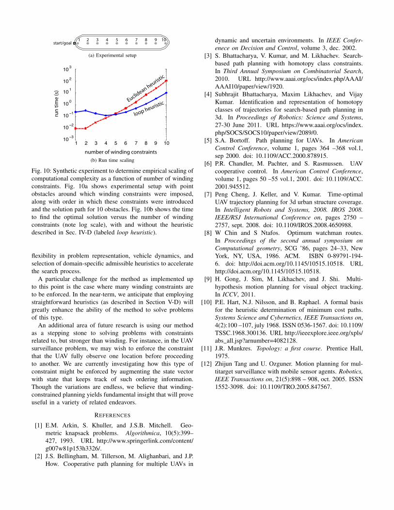
In order to study the computational efficiency of the method,we applied it to a synthetic example where we varied just thenumber of regions with winding constraints. The experimentalscenario is depicted in Fig. 10. In the nth trial, we used ourmethod to find a loop around the regions labeled 1, 2, . . . n,winding once in the positive direction around each. This wasconducted both using the heuristic described in Sec. IV-D—which we will refer to as the loop heuristic—and using theEuclidean distance-to-goal heuristic.

Fig. 10b shows a clearly asymptotic exponential scalingin the run time as a function of the number of windingconstraints for both heuristics. The loop heuristic, however,exhibits a significantly more shallow slope in the log plot; for10 constraints, the Euclidean distance heuristic is slower bya factor of 10. An interesting observation is that the perfor-mance of the loop heuristic was relatively insensitive to thenumber of constraints up to about six, at which point planningtimes increased significantly. For a very small number ofconstraints, the Euclidean distance heuristic outperformed theloop heuristic by a large margin, which we attribute to thesmaller overhead of the Euclidean heuristic.

The reason for the observed exponential scaling is that thesearch ultimately begins to explore many different combina-tions of windings around different obstacles. As we increasethe number of constraints, the number of plausible windingstates (and by extension, the open list) grows exponentially.The loop heuristic was able to compensate for this effectsomewhat, but not completely. We also observed in experimenswith constraints winding multiple times around each region,that the performance of the loop heuristic deteriorated. This isto be expected, as it does not take into account the effect ofmultiple windings.

We are currently investigating different avenues to enablescaling to yet larger numbers of winding constraints. Onesimple enhancement would be to prune the search whenwinding angles become too large (a similar strategy was usedin [9]), at the expense of losing the completeness guarantee ofthe search. Also, as noted in Section III, certain variants of thegeometric knapsack problem in computational geometry may

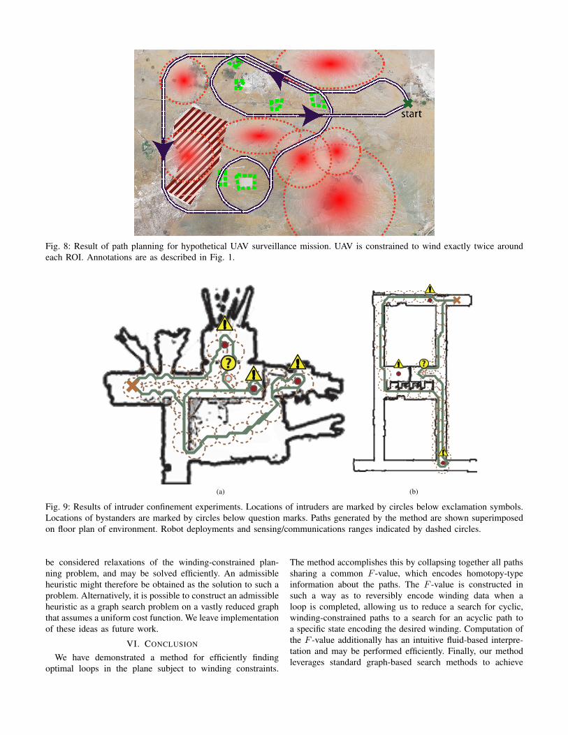
Fig. 8: Result of path planning for hypothetical UAV surveillance mission. UAV is constrained to wind exactly twice aroundeach ROI. Annotations are as described in Fig. 1.

?

(a)

?

(b)

Fig. 9: Results of intruder confinement experiments. Locations of intruders are marked by circles below exclamation symbols.Locations of bystanders are marked by circles below question marks. Paths generated by the method are shown superimposedon floor plan of environment. Robot deployments and sensing/communications ranges indicated by dashed circles.

be considered relaxations of the winding-constrained plan-ning problem, and may be solved efficiently. An admissibleheuristic might therefore be obtained as the solution to such aproblem. Alternatively, it is possible to construct an admissibleheuristic as a graph search problem on a vastly reduced graphthat assumes a uniform cost function. We leave implementationof these ideas as future work.

VI. CONCLUSION

We have demonstrated a method for efficiently findingoptimal loops in the plane subject to winding constraints.

The method accomplishes this by collapsing together all pathssharing a common F -value, which encodes homotopy-typeinformation about the paths. The F -value is constructed insuch a way as to reversibly encode winding data when aloop is completed, allowing us to reduce a search for cyclic,winding-constrained paths to a search for an acyclic path toa specific state encoding the desired winding. Computation ofthe F -value additionally has an intuitive fluid-based interpre-tation and may be performed efficiently. Finally, our methodleverages standard graph-based search methods to achieve

start/goal1 2 3 4 5 6 7 8 9 10

(a) Experimental setup

1 2 3 4 5 6 7 8 9 1010 −3

10 −2

10 −1

10 0

10 1

10 2

10 3

run

time

(s)

number of winding constraints

Euclidean heuristic

loop heuristic

(b) Run time scaling

Fig. 10: Synthetic experiment to determine empirical scaling ofcomputational complexity as a function of number of windingconstraints. Fig. 10a shows experimental setup with pointobstacles around which winding constraints were imposed,along with order in which these constraints were introducedand the solution path for 10 obstacles. Fig. 10b shows the timeto find the optimal solution versus the number of windingconstraints (note log scale), with and without the heuristicdescribed in Sec. IV-D (labeled loop heuristic).

flexibility in problem representation, vehicle dynamics, andselection of domain-specific admissible heuristics to acceleratethe search process.

A particular challenge for the method as implemented upto this point is the case where many winding constraints areto be enforced. In the near-term, we anticipate that employingstraightforward heuristics (as described in Section V-D) willgreatly enhance the ability of the method to solve problemsof this type.

An additional area of future research is using our methodas a stepping stone to solving problems with constraintsrelated to, but stronger than winding. For instance, in the UAVsurveillance problem, we may wish to enforce the constraintthat the UAV fully observe one location before proceedingto another. We are currently investigating how this type ofconstraint might be enforced by augmenting the state vectorwith state that keeps track of such ordering information.Though the variations are endless, we believe that winding-constrained planning yields fundamental insight that will proveuseful in a variety of related endeavors.

REFERENCES

[1] E.M. Arkin, S. Khuller, and J.S.B. Mitchell. Geo-metric knapsack problems. Algorithmica, 10(5):399–427, 1993. URL http://www.springerlink.com/content/g007w81p153h3326/.

[2] J.S. Bellingham, M. Tillerson, M. Alighanbari, and J.P.How. Cooperative path planning for multiple UAVs in

dynamic and uncertain environments. In IEEE Confer-enece on Decision and Control, volume 3, dec. 2002.

[3] S. Bhattacharya, V. Kumar, and M. Likhachev. Search-based path planning with homotopy class constraints.In Third Annual Symposium on Combinatorial Search,2010. URL http://www.aaai.org/ocs/index.php/AAAI/AAAI10/paper/view/1920.

[4] Subhrajit Bhattacharya, Maxim Likhachev, and VijayKumar. Identification and representation of homotopyclasses of trajectories for search-based path planning in3d. In Proceedings of Robotics: Science and Systems,27-30 June 2011. URL https://www.aaai.org/ocs/index.php/SOCS/SOCS10/paper/view/2089/0.

[5] S.A. Bortoff. Path planning for UAVs. In AmericanControl Conference, volume 1, pages 364 –368 vol.1,sep 2000. doi: 10.1109/ACC.2000.878915.

[6] P.R. Chandler, M. Pachter, and S. Rasmussen. UAVcooperative control. In American Control Conference,volume 1, pages 50 –55 vol.1, 2001. doi: 10.1109/ACC.2001.945512.

[7] Peng Cheng, J. Keller, and V. Kumar. Time-optimalUAV trajectory planning for 3d urban structure coverage.In Intelligent Robots and Systems, 2008. IROS 2008.IEEE/RSJ International Conference on, pages 2750 –2757, sept. 2008. doi: 10.1109/IROS.2008.4650988.

[8] W Chin and S Ntafos. Optimum watchman routes.In Proceedings of the second annual symposium onComputational geometry, SCG ’86, pages 24–33, NewYork, NY, USA, 1986. ACM. ISBN 0-89791-194-6. doi: http://doi.acm.org/10.1145/10515.10518. URLhttp://doi.acm.org/10.1145/10515.10518.

[9] H. Gong, J. Sim, M. Likhachev, and J. Shi. Multi-hypothesis motion planning for visual object tracking.In ICCV, 2011.

[10] P.E. Hart, N.J. Nilsson, and B. Raphael. A formal basisfor the heuristic determination of minimum cost paths.Systems Science and Cybernetics, IEEE Transactions on,4(2):100 –107, july 1968. ISSN 0536-1567. doi: 10.1109/TSSC.1968.300136. URL http://ieeexplore.ieee.org/xpls/abs all.jsp?arnumber=4082128.

[11] J.R. Munkres. Topology: a first course. Prentice Hall,1975.

[12] Zhijun Tang and U. Ozguner. Motion planning for mul-titarget surveillance with mobile sensor agents. Robotics,IEEE Transactions on, 21(5):898 – 908, oct. 2005. ISSN1552-3098. doi: 10.1109/TRO.2005.847567.