the local bootstrap for markov processesbhansen/718/paparoditispolitisnp.pdfblocks-of-blocks...

Journal of Statistical Planning andInference 108 (2002) 301–328

www.elsevier.com/locate/jspi

The local bootstrap for Markov processes�

Efstathios Paparoditisa, Dimitris N. Politisb; ∗aDepartment of Mathematics and Statistics, University of Cyprus, P.O. Box 20537,

CY 1678 Nicosia, CyprusbDepartment of Mathematics, University of California, San Diego, La Jolla, CA 92093-0112, USA

Abstract

A nonparametric bootstrap procedure is proposed for stochastic processes which follow a gen-eral autoregressive structure. The procedure generates bootstrap replicates by locally resamplingthe original set of observations reproducing automatically its dependence properties. It avoids aninitial nonparametric estimation of process characteristics in order to generate the pseudo-timeseries and the bootstrap replicates mimic several of the properties of the original process. Ap-plications of the procedure in nonlinear time-series analysis are considered and theoreticallyjusti.ed; some simulated and real data examples are discussed.c© 2002 Published by Elsevier Science B.V.

MSC: primary 62G09; 62M05; secondary 62M10

Keywords: Markov dependence; Nonlinear time series; Resampling; Time reversibility

1. Introduction

The present paper introduces a new resampling procedure, namely the local boot-strap, which is applicable in the setting of strictly stationary, real-valued stochasticprocesses {Xt; t = 1; 2; : : :} that follow a general (.nite order) Markovian structure,i.e., a dependence structure where for every t ∈N and every Borel set A ⊂ R; Xt

depends on the past only through the previous p values, i.e.,

P(Xt+1 ∈A|Xj; j6 t) = P(Xt+1 ∈A|Xj; t − p + 16 j6 t):

Although the class of processes to which our procedure is applicable will be moreprecisely described in the next section, we mention here that it is large enough to

� Research partially supported by NSF Grant DMS-97-03964.∗ Corresponding author.E-mail address: [email protected] (D.N. Politis).

0378-3758/02/$ - see front matter c© 2002 Published by Elsevier Science B.V.PII: S0378 -3758(02)00315 -4

302 E. Paparoditis, D.N. Politis / Journal of Statistical Planning and Inference 108 (2002) 301–328

include several of the commonly used nonlinear models in time-series analysis. Animportant member of this class is, for instance, the class of nonlinear, conditionallyheteroscedastic, autoregressive processes de.ned by

Xt = m(Xt−1; Xt−2; : : : ; Xt−p) + v(Xt−1; Xt−2; : : : ; Xt−p) jt ; t = 1; 2; : : : ; (1)

where the noise process {jt ; t¿ 1} is a sequence of i.i.d. zero mean random vari-ables satisfying certain assumptions and m(·) and v(·) are smooth functions (generallyunknown). Note that model (1) includes several of the familiar nonlinear parametricmodels; see Tong (1990) and TjHstheim (1994) for details. However, (1) is not ex-plicitly assumed in the following, i.e., the Markov class of processes to which ourprocedure is applicable is richer than model (1).

The local bootstrap scheme proposed in this paper involves resampling the orig-inal data points X1; X2; : : : ; XT to form pseudoseries X ∗

1 ; X ∗2 ; : : : ; X ∗

T from which thestatistics of interest are recalculated. To motivate the idea underlying the procedureproposed, consider the particular case where {Xt} indeed follows the general autore-gressive structure (1) with p = 1, and let X1; X2; : : : ; XT be the observed series. Giventhe value assumed by the process at time t, i.e., given Xt , consider the problem ofobtaining a replicate of the value assumed at t + 1 when m(·) and v(·) are unknown.To proceed, assume that an observation Xs ∈{X1; X2; : : : ; XT−1}, with s �= t exists whichis close to Xt , i.e., |Xt −Xs|6 b, for some small b¿ 0. Then for m(·) and v(·) smoothfunctions, diDerences between the subsequent values Xt+1 and Xs+1 are mainly due todiDerences in the unobserved errors, i.e., jt+1 and js+1. To see this, suppose that mand v have bounded .rst-order derivatives and that jt has .nite variance; a Taylorseries expansion yields

Xs+1 = m(Xs) + v(Xs)js+1 = m(Xt) + v(Xt)js+1 + OP(b);

i.e., for b close to zero, Xs+1 can be thought to have been generated by the samestochastic diDerence equation as Xt+1 = m(Xt) + v(Xt)jt+1 but with a diDerent errorterm (js+1 instead of jt+1). Since the above consideration is true for all observedvalues which have the same property as Xs+1, i.e., the property that their precedingvalue in the original data sequence is b-close to Xt , a replicate X ∗

t+1 of Xt+1 can beobtained by randomly choosing a value from the set of observations

{Xs+1: |Xt − Xs|6 b and 16 s6T − 1}:In choosing X ∗

t+1 from the above set, an appropriate probability distribution, which wewill term the resampling kernel, is used. Thus starting at t = 1 by some appropriatelychosen initial value X ∗

1 , subsequent replicates X ∗2 ; X ∗

3 ; : : : ; X ∗T can be obtained by ap-

plying the above local resampling scheme at each stage of the resampling process. Itcan then be shown that for an important class of statistical problems and under cer-tain regularity conditions, asymptotically valid inference can be obtained by letting theresampling width b = b(T ) → 0 as the sample size T increases but in such a waythat the number of observations falling in the set from which bootstrap replicates areobtained goes to in.nity.

Bootstrapping time-series data has received considerable interest in recent years. Asa follow-up to the i.i.d. bootstrap of Efron (1979), several diDerent approaches for

E. Paparoditis, D.N. Politis / Journal of Statistical Planning and Inference 108 (2002) 301–328 303

bootstrapping stationary observations have been proposed in the literature. Let us justmention here among others, the ‘residual bootstrap’ (cf. Freedman, 1984; Efron andTibshirani, 1986), the block bootstrap (cf. KJunsch, 1989; Liu and Singh, 1992), theblocks-of-blocks bootstrap (cf. Politis and Romano, 1992), the stationary bootstrap (cf.Politis and Romano, 1994), the frequency domain bootstrap (cf. Franke and HJardle,1992); see Shao and Tu (1995) for an overview of those methods.

The local bootstrap proposal of this paper is perhaps more akin to a bootstrap pro-cedure for (.rst order) Markov processes suggested by Rajarshi (1990). In that proce-dure bootstrap replicates are obtained by using the nonparametrically estimated one-steptransition density function. To be more precise, for p = 1 and X ∗

t given, a subsequentvalue X ∗

t+1 is obtained as X ∗t+1 ∼ f Xt+1|Xt

(· |X ∗t ) where f Xt+1|Xt

(· |X ∗t ) is a nonpara-

metric (kernel) estimator of the unknown conditional density function fXt+1|Xt (· |X ∗t )

of the process. Compared to the bootstrap procedure of Rajarshi (1990), the local re-sampling procedure proposed in this paper is simpler, easier to implement and avoidsthe nonparametric estimation of the conditional density fXt+1|Xt (·|X ∗

t ).In essence, our local bootstrap implicitly performs an estimation of the one-step

transition distribution as opposed to Rajarshi’s (1990) (explicit) estimation of the tran-sition density by nonparametric smoothing of the transition distribution. We show that,similarly to the question “to smooth or not to smooth” in the classical i.i.d. bootstrap(cf. Efron and Tibshirani, 1993, and the references therein), this extra smoothing istypically unnecessary for the bootstrap to work in the Markovian case. As an added fea-ture, our local bootstrap pseudo-series consist of (particular) reshuOings of the originaldata points, the reshuOing being done of course according to a particular probabilitymechanism. This constitutes a further similarity of the local bootstrap to Efron’s (1979)classical i.i.d. bootstrap; in eDect, Efron’s (1979) i.i.d. bootstrap can be considered asa special case of our local bootstrap if we allow the Markovian order p to be zero.

Under model class (1), there exists a residual-based procedure investigated by Frankeet al. (1996) that begins with nonparametric estimation of m(·) and v(·), and a sub-sequent i.i.d. resampling of the estimated residuals; cf. also Auestad and TjHstheim(1991). In contrast to this approach our local bootstrap scheme does not attempt toreduce the problem to i.i.d. resampling of residuals but involves resampling the originaldata points to form the pseudo-time series. Again, it has the advantage of side-steppingsuch initial smoothing problems, and at the same time it is valid for a class of stochas-tic processes that is wider than (1). As a .nal point, note that the local bootstrap isrelated to the resampling algorithms proposed by Shi (1991) in the context of i.i.d.regression, by Falk and Reiss (1992) in the context of bootstrapping conditional curvesand in an ad hoc manner by Lall and Sharman (1996) in the context of hydrologicaltime series, and by Chan et al. (1997) in the context of ecological series.

The paper proceeds as follows. In Section 2, the local resampling method is de-scribed. Its .nite sample as well as its asymptotic properties are discussed in greatdetail in Section 3. The properties of the local bootstrap derived in this section makeit potentially applicable to a variety of inference problems. Section 4 deals withsuch applications of the local bootstrap; here the resampling procedure proposed isused to conduct statistical inference pertaining to linear statistics, as well as analyzethe lag-reversibility properties of a time series. Some practical aspects of selecting


the resampling parameters—in particular, the resampling width b—are discussed inSection 5. Applications to simulated and real data are given in this section as well.Section 6 contains some concluding remarks while all technical proofs are deferred toAppendix A.

2. The local bootstrap

2.1. Basic notation and assumptions

We begin with an assumption which speci.es precisely the class of stochastic process{Xt; t¿ 1} considered. We denote by Bp the Borel �-algebra over Rp.

(A1) There exists a positive integer p¡∞ such that the stochastic processY = {Yt ; t¿ 1} with Yt de.ned by Yt = (Xt; Xt−1; : : : ; Xt−p+1), forms an aperiodic,strictly stationary and geometrically ergodic Markov chain on (Rp;Bp).

We assume that the integer p is the smallest possible for which (A1) is satis.ed.Note that the aperiodicity assumption together with geometric ergodicity implies thata unique invariant probability measure �Y on Rp exists, which is the stationary dis-tribution of Y. The assumption of strict stationarity implies then that L(Y1) = �Ywhere L(Y1) denotes the law of the starting value Y1 = (X1; X0; : : : ; X2−p). Further-more, geometric ergodicity together with stationarity implies that the Markov chain{Xt; t¿ 1} is geometrically strong mixing (i.e., �-mixing), since it is geometricallyabsolutely regular (i.e., �-mixing); cf. Doukhan (1995, Chapter 2.4).

Assumption (A1) is general enough in that it is ful.lled by several of the commonlyused nonlinear time-series models. In fact, there is a large amount of literature dealingwith stationarity and geometric ergodicity results for diDerent nonlinear time-seriesmodels that admit a Markovian dependence structure; cf., among others, Tong (1990),TjHstheim (1990), Ango Nze (1992) and Meyn and Tweedie (1993).

Denote in the following by F(·) the stationary distribution of Xt , the existence ofwhich is ensured by the fact that the sample paths of {Xt; t¿ 1} are those of the .rstcomponent of Yt . Note that F(x)=FY(x;∞; : : : ;∞) where FY(y)=�Y((−∞; y]) is theunique solution of

FY(y) =∫

FY(y|x) dFY(x); x∈Rp (2)

and FY(· |x) is the one-step transition distribution function of Y, i.e.,

FY(y|x) = P(Yt+16 y|Yt = x) for y; x∈Rp:

We denote in the following by F(y|x) the one-step transition distribution function ofXt , i.e.,

F(y|x) = P(Xt+16y|Yt = x):

By (A1) the transition distribution function F(y|x) uniquely characterizes the law of thestationary process {Xt; t¿ 1}. Now, let fYt (·) be the stationary density, fXt+1|Yt (·|x)the one-step transition density, fXt+1Yt (·; x)=fXt+1|Yt (·|x)fYt (x) and denote by ‖ ·‖ theEuclidean norm.


(A2)

(i) FY(·) and F(·|x) are absolutely continuous with respect to Lebesgue measure onRp and R and have bounded densities fYt (·) and fXt+1|Yt (·|x), respectively.

(ii) For x1; x2 ∈Rp and y∈R ∪ {∞},

∣∣∣∣∫ y

−∞fXt+1 ;Yt (z; x1) dz −

∫ y

−∞fXt+1 ;Yt (z; x2) dz

∣∣∣∣6L(y)‖x1 − x2‖;

where inf y L(y)¿ 0 and supy L(y) = L¡∞.(iii) For y1; y2 ∈R; |fXt+1|Yt (y1|x)−fXt+1|Yt (y2|x)|6C(x)|y1 − y2| where C(x)¿ 0

and supx∈Rp C(x) = C ¡∞.

The smoothness assumptions on the stationary and on the one-step transition densitiesimposed above are very common in nonparametric estimation and are needed hereto ensure consistency of the empirical characteristics used to generate the bootstrappseudo-series.

(A3) A compact subset S of R exists such that Xt ∈ S a.s. Furthermore, fXt+1|Yt (·|x)¿ 0 for every x∈S, where S denotes the p-fold Cartesian product of S.

Note that the compactness of the support of f in (A3) is a rather technical as-sumption that can be weakened by simultaneously strengthening other requirements;see Remark 3.2 for a discussion of this point.

To set up the local resampling procedure, we .rst introduce a resampling kernelW (·), i.e., an appropriate probability density on Rp, which is used in local resamplingof the observations. This resampling kernel satis.es the following assumptions.

(B1) W (·) is a bounded, (.rst order) Lipschitz continuous and symmetric probabil-ity density on Rp satisfying W (u)¿ 0 for all u. Furthermore,

∫uW (u) du = 0 and∫ ‖u‖W (u) du¡∞.

For any real number c¿ 0 we set in the following Wc(·)= c−pW (·=c). Furthermore,the notations f(·) and f(·|x) for the stationary density fY(·) and the one-step transitiondensity fXt+1|Yt (·|x) will be also used in the sequel as convenient short-hands.

2.2. The resampling scheme

The resampling algorithm proposed generates bootstrap pseudo-series X ∗1 ; X ∗

2 ; : : : ; X ∗N

where in general, the length N of the bootstrap series is not necessary equal to T ,although N = T is a natural choice for statistical applications. Denote by Y∗

t the rowvector Y∗

t =(X ∗t ; X

∗t−1; : : : ; X

∗t−p+1). The local resampling algorithm generating the boot-

strap replicates can then be described by the following two steps:

1. Select a resampling width b = b(T )¿ 0 and a set of p starting values Y∗p =

(X ∗1 ; X ∗

2 ; : : : ; X ∗p ).

2. For any t+1∈{p+1; p+2; : : : ; N} suppose that Y∗t has been generated already. Let J

be a discrete random variable taking its values in the set Np;T−1={p;p+1; : : : ; T−1}


with probability mass function given by

P(J = s) = Wb(Y∗t − Ys)

/ ∑m∈Np;T−1

Wb(Y∗t − Ym) (3)

for s∈Np;T−1. The bootstrap replicate X ∗t+1 is then de.ned by X ∗

t+1 = XJ+1.

According to the above resampling scheme and based on the resampling kernel Wand the resampling width b, the bootstrap procedure assigns at any time point t + 1and any assumed value of Y∗

t diDerent resampling probabilities to the data pointsXp+1; Xp+2; : : : ; XT . These probabilities depend on how close to Y∗

t is the set of eachpoint’s preceding p values (in the original data sequence). In so doing the procedureactually de.nes for each time point t ∈{p + 1; p + 2; : : :} a local neighborhood fromwhich the value X ∗

t+1 is obtained; resampling from the successors of the values lyingin this neighborhood justi.es calling this procedure a local bootstrap.

Remark 2.1. Some variations of this procedure can be obtained by varying the wayof choosing the starting values X ∗

1 ; X ∗2 ; : : : ; X ∗

p . For instance; one possibility is to startresampling by setting Y∗

p = Yp or Y∗p ∈{Yt : p6 t6T − 1}. Another possibility is

to allow Y∗p to take; with a predetermined probability distribution any value from the

set of values {(Xt1 ; Xt2 ; : : : ; Xtp): p+ 16 tj6T and j = 1; 2; : : : ; p}; this predetermineddistribution could well be the stationary distribution of the corresponding bootstrapMarkov chain in which case the bootstrap series would itself be stationary as Theorem3.1 indicates.

Example 2.1. Before proceeding with the properties of the local resampling procedureand for the purposes of illustration we apply it to the well-known series of WJolfersunspot numbers; cf. Tong (1990) for a description and discussion of this famous series.Fig. 1 shows the original series and a bootstrap replicate obtained using Y∗

p = Yp, anautoregressive order of p = 9, the Gaussian product kernel as resampling kernel anda resampling width b according to Eq. (13) in Section 5. Note that an autoregressiveorder of p = 9 has been suggested as appropriate for this series by TjHstheim andAuestad (1994). As it is seen from this .gure, the local bootstrap procedure managesto reproduce quite satisfactorily the main characteristics of this series.

3. Properties of the local bootstrap

3.1. Case of :xed T

According to the proposed resampling scheme, for any .xed length T of the ob-served series, the sequence of bootstrap random variables {X ∗

t ; t = 1; 2; : : :} evolvesthrough the ‘numbered states’ X1; X2; : : : ; XT following a certain dependence (autore-gressive) structure. In particular, we have for any positive integer N ¿p and any set


Fig. 1. Original series of sunspot numbers (top) and a bootstrap replication using the local resampling schemewith p = 9, the Gaussian product resampling kernel and a resampling width selected using Eq. (13).

{x1; x2; x3; : : : ; xN} with xi ∈{X1; X2; : : : ; XT} that

P(X ∗1 = x1; X ∗

2 = x2; : : : ; X ∗N = xN ) = P0(Y∗

p = xp)N−1∏t=p

P(X ∗t+1 = xt+1|Y∗

t = xt);

where for xt =(xt ; xt−1; : : : ; xt−p+1) and j∈{p;p+1; : : : ; T−1}, P(X ∗t+1 =Xj+1|Y∗

t =xt)is the transition kernel given by

P(X ∗t+1 = Xj+1|X ∗

t = xt ; X ∗t−1 = xt−1; : : : ; X ∗

t−p+1 = xt−p+1)

=Wb(xt − Yj)∑T−1

m=p Wb(xt − Ym): (4)

Note that P0 denotes the probability function determining the choice of the initialvalues Y∗

p =(X ∗1 ; X ∗

2 ; : : : ; X ∗p ). Thus, apart from the starting values and conditionally on

the observed sequence X1; X2; : : : ; XT , the bootstrap series X ∗p+1; X

∗p+2; : : : ; is the sample

path of the .rst component of the p-dimensional process Y∗T ={Y∗

t ; t¿p+1}, whereY∗

t = (X ∗t ; X

∗t−1; : : : ; X

∗t−p+1) is generated by a discrete and temporarily homogeneous

.rst-order Markov chain that takes its values in the discrete state space ET = XpT .

Here XpT denotes the Cartesian product of p copies of XT = {Xp+1; Xp+2; : : : ; XT}.

Furthermore, the law of {X ∗t ; t¿p + 1} is the law of the .rst component of Y∗

t .The following theorem characterizes precisely the properties of this chain. It enablesus to use Markov chain theory in order to investigate several of the properties of theprobabilistic mechanism generating the local bootstrap replicates.

Theorem 3.1. For X1; X2; : : : ; XT given; and for every b¿ 0 :xed and any resamplingkernel W (·) satisfying assumption (B1); there exists with probability one an integer


t0 ∈N such that for all t¿ t0 the Markov chain Y∗T = {Y∗

t ; t¿ t0} generating thebootstrap values X ∗

t is positive recurrent; irreducible and aperiodic.

Note that the particular value of t0 depends on the choice of the starting values Y∗p.

Therefore, and for the sake of simplicity, we assume in the following that t0 = p + 1.

Remark 3.1. Although not stated explicitly; the probabilistic behavior of thebootstrap Markov chain Y∗

T depends on the resampling kernel W (·) and more im-portantly on the resampling width b. In particular; for T .xed and b → 0; we haveP(X ∗

t+1 = Xj+1|Y∗t = x) → #j+1; l+1 where #j+1; l+1 is Kronecker’s delta and l the index

of the observation in the original data sequence assumed by X ∗t ; i.e.; X ∗

t = Xl. In thiscase; the bootstrap process de.ned by the above local resampling scheme; reproduces(almost surely) the original sequence Xp+1; Xp+2; : : : ; XT of observations. On the otherextreme; for b → ∞; P(X ∗

t+1 = Xl+1|Y∗t = x) → 1=(T − p); i.e.; in that case the local

resampling scheme approaches an i.i.d. resampling from the set {Xp+1; Xp+2; : : : ; XT}.Clearly; to mimic the variability of the original series by simultaneously reproducingits (Markovian) dependence characteristics; b should lie between these two extremes.

Theorem 3.1 implies that for every T , a unique, discrete, invariant probability mea-sure �∗

T on ET exists, which is the stationary distribution of the bootstrap chain Y∗T .

Furthermore, a constant %∗T ∈ (0; 1), that in general depends on the values X1; : : : ; XT

but not on anything else, exists such that ‖P(k)(x; ·)−�∗T (·)‖V =o(%∗

k

T ) where P(k)(x; ·)denotes the k-step transition kernel of Y∗

t , i.e., P(k)(x; A) = P(Y∗t+k ∈A|Y∗

t = x) forA∈B(ET ). In this notation ‖ · ‖V states for the total variation norm while B(ET ) de-notes the �-.eld of all countable subsets of ET ; cf. Meyn and Tweedie (1993). Notethat the discrete bootstrap Markov chain Y∗

T generating the bootstrap replicates satis.esDoeblin’s condition D; cf. Doob (1953, p. 192). Together with the aperiodicity of Y∗

Tthis implies that for every T; {X ∗

t ; t¿ 1} is uniformly mixing, i.e., ’∗T (n) → 0 as

n → ∞ where

’∗T (n) = sup

A∈F∗p1 ;B∈F∗∞

p+n

|P∗(B|A) − �∗T (B)| (5)

and F∗p

1 = �(X ∗1 ; X ∗

2 ; : : : ; X ∗p ) and F∗∞

p+n = �(X ∗p+n; X

∗p+n+1; : : :) are the �-algebras

generated by X ∗1 ; X ∗

2 ; : : : ; X ∗p and X ∗

p+n; X∗p+n+1; : : : ; respectively; see Doukhan (1994,

p. 88).Clearly, if L(Y∗

1 ) = �∗T the bootstrap process {X ∗

t ; t¿ 1} is strictly stationary, thestationary distribution function of which is denoted in the following by F∗

T (·). FromTheorem 3.1 we then have F∗

T (y) = F∗Y;T (y;∞; : : : ;∞) where F∗

Y;T (y) = �∗T ((−∞; y])

and F∗Y;T (y) is uniquely determined by the equation

F∗Y;T (y) =

∫F∗Y;T (y|x) dF∗

Y;T (x): (6)

F∗Y;T (·|x) appearing in the above equation is the one-step transition distribution function

given by

F∗Y;T (y |x) = P(Y∗

t+16 y |Y∗t = x) for x∈ET :


3.2. Case of increasing T

Our discussion was so far restricted to the case of a .xed length T of the observedseries. We now turn to the probabilistic properties of the bootstrap process {X ∗

t ; t¿ 1}as the length T of the observed series increases. The asymptotic results obtained in thefollowing are derived under the assumption that the local neighborhood from whichobservations are resampled is getting narrower as the sample sizes increases but insuch a way that the number of observations ‘falling’ in this neighborhood increases toin.nity. To be more precise, we assume that

(B2) b � T−# with 0¡#¡ 1=(2p).The notation b � T−# means that constants c1 and c2 exist such that 0¡c16 bT#

6 c2 ¡∞ for all T large enough.Consider .rst the behavior of the one-step transition distribution function F∗

T (y|x) =P(X ∗

t+16y|Y∗t = x) governing the law of the bootstrap process and note that

F∗T (y|x) =

T−1∑j=p

1(−∞;y](Xj+1)P(X ∗t+1 = Xj+1|Y∗

t = x)

=

∑T−1j=p 1(−∞;y](Xj+1)Wb(x− Yj)∑T−1

m=p Wb(x− Ym)(7)

is used to mimic the one-step transition distribution function

F(y|x) =∫

1(−∞;y](z)fXt+1|Yt (z|x) dz: (8)

The following result which is essential in obtaining several of the properties of thelocal bootstrap replicates can then be established.

Theorem 3.2. Under assumptions (A1)–(A3) and (B1)–(B2) we have as T → ∞supy∈R

supx∈S

|F∗T (y|x) − F(y | x)| → 0 a:s:

The importance of the above result lies in the fact that, apart from the choice ofthe initial values, the statistical model associated with {Xt; t¿ 1} is completely speci-.ed by means of the one-step transition distribution function F(y|x). In fact, F(y|x)together with the Markov property determines uniquely all the .nite-dimensional dis-tributions and therefore the whole dependence structure of {Xt; t¿ 1}. Similarly, thewhole dependence structure of the local bootstrap series is determined by the bootstrapone-step transition distribution function F∗

T (·|x). Now, since under our assumptions,F∗T (y|x) → F(y|x) strongly and uniformly in both arguments as T → ∞, the above

result justi.es theoretically the use of the local bootstrap series in order to reproducethe dependence characteristics of the stochastic process generating the observations.

Remark 3.2. From a technical point of view; assumption (A3) on a bounded supportof f(·) can be avoided by extending the result of Theorem 3.2 to a strong uniform


convergence of F∗T (·|x) to F(·|x) over compact subsets ST of Rp which expand to

all of Rp as the sample size T increases. In particular; let ST be the ball in Rp

with center the origin and radius RT and let RT = T, for some ,¿ 0. Assume furtherthat inf x∈ST f(x)¿T−% for some %¿ 0. It can then be shown along the same linesas in the proof of Theorem 3.2 (cf. also Theorem 3.2 of Roussas; 1988) that if theresampling width b is chosen so that b � T−# with 0¡%+#p¡ 1=2; then as T → ∞

supy∈R

supx∈ST

|F∗T (y | x) − F(y | x)| → 0 a:s:

This implies that in case of an unbounded support of f(·) and in order to obtain anasymptotically valid procedure; resampling should be done from a ‘truncated’ sequenceof observations; denoted by X 1; X 2; : : : ; X T ; where X t = Xt if |Xt |6RT and X t =sgn (Xt)RT if |Xt |¿RT and where the truncation level RT tends to ∞ at the rategiven above as T → ∞. We stress here the fact that such a truncation changes solelythe state space of the bootstrap Markov chain and does not aDect its Markov propertiesand characteristics.

The properties of the bootstrap stationary distribution function F∗T are summarized

in the following theorem.

Theorem 3.3. Under the same assumptions as in Theorem 3.2; we have

supy∈R

|F∗T (y) − F(y)| → 0 a:s:

Note that once a bootstrap realization has been obtained, the pseudo-observationsX ∗

1 ; X ∗2 ; : : : ; X ∗

N can be used to recalculate statistics of interest. In order to be able toobtain asymptotic bounds of covariances and to establish the large sample validity ofthe local bootstrap for a large class of statistical inference problems, we characterize inthe following the asymptotic behavior of the weak dependence of the local bootstrapseries by means of the --mixing coeTcient. This coeTcient is de.ned as follows:Let {Zt; t ∈N} be a sequence of random variables and let FJ

1 = �(Zk ; 16 k6 J )and F∞

J+n = �(Zk ; J + n6 k ¡∞) be the �-algebras generated by Z1; Z2; : : : ; ZJ andZJ+n; ZJ+n+1; : : :, respectively. The --mixing coeTcient is then de.ned by

-(n)=sup{|Corr(/1; /2)|; /1 beingFJ1 -measurable; /2 beingF∞

J+n -measurable

with E|/1|2 ¡∞; E|/2|2 ¡∞ and J¿ 1}:The random sequence {Zk} is called --mixing if -(n) → 0 as n → ∞. Note that--mixing implies �-mixing; cf. Doukhan (1994, p. 20). The following theorem canthen be established, where as before we de.ne:

-∗(n)=sup{|Corr(/1; /2)|; /1 beingF∗J1 -measurable; /2 beingF∗∞

J+n -measurable

with E|/1|2 ¡∞; E|/2|2 ¡∞ and J¿ 1};where F∗J

1 ;F∗∞J+n were de.ned in Eq. (5).


Theorem 3.4. Under the assumptions of Theorem 3.2 and conditionally on X1; X2; : : : ;XT ; T0 ∈N exists such that for all T¿T0 the -∗-mixing coe<cient of the bootstrapseries {X ∗

t ; t¿ 1} satis:es -∗T (n)6 %n; where the constant %∈ (0; 1) is independent

of T .

4. Applications

4.1. Linear statistics

In this section we deal with applications of the local bootstrap procedure in estimatingthe sampling properties of linear statistics de.ned by

2T =1

T − m + 1

T−m+1∑t=1

g(Xt; Xt+1; : : : ; Xt+m−1); (9)

where g :Rm → R is a continuous function and m∈N. To simplify notation, let Zt =g(Xt; Xt+1; : : : ; Xt+m−1), denote by 2g the mean 2g = E[Zt] which is assumed to existand set 2 = 2g. Under our assumptions on the process {Xt} and if E|Zt |2+4 ¡∞ forsome 4¿ 0 it follows by Theorem 1.7 of Ibragimov (1962) that

�2g = lim

T→∞Var(

√T 2T ) = Var(Z1) + 2

∞∑5=1

Cov(Z1; Z1+5)¿ 0

exists. Furthermore,

L(√T (2T − 2)) ⇒ N (0; �2

g);

where L(Y ) denotes the law of the random variable Y and ⇒ stands for weak con-vergence. Now, as an alternative to the normal approximation to

√T (2T − 2), or just

to be able to estimate the limiting variance �2g, we propose in the following to use the

bootstrap distribution of the statistic√T (2

∗T − 2 ∗) where 2

∗T is de.ned by

2∗T =

1T − m + 1

T−m+1∑t=1

g(X ∗t ; X

∗t+1; : : : ; X

∗t+m−1) (10)

and 2 ∗ =E∗[g(X ∗t ; X

∗t+1; : : : ; X

∗t+m−1)]. Here E∗ denotes expectation with respect to the

bootstrap distribution.The following theorem shows that the bootstrap approximation proposed ‘works’

asymptotically in the sense that �∗2

g;T = Var∗(√T 2

∗T ) converges to the correct limit

variance �2g, and that the law of

√T (2

∗T − 2 ∗) (conditionally on the data) is close to

the law of√T (2T−2) with high probability, if the sample size T is large enough. In this

theorem, Kolmogorov’s distance, de.ned by d0(P;Q)=supx∈R |P(X 6 x)−Q(X 6 x)|,is used in order to estimate the distance between probability measures P and Q.


Theorem 4.1. Assume that (A1)–(A3) and (B1)–(B2) are ful:lled. For g continuousand E|Zt |2+4 ¡∞ for some 4¿ 0; we have as T → ∞1. �∗2

g;T → �2g

and2. d0{L(

√T (2

∗T − 2 ∗)|X1; X2; : : : ; XT );L(

√T (2T − 2))} → 0;

both convergences being valid with probability one.

The large sample validity of the local bootstrap procedure can be also established formultivariate versions of (9), i.e., for linear statistics where g is a continuous mappingfrom Rm into Rs, and s¿ 1. In particular, for x∈Rm, let g(x) = (g1(x); : : : ; gs(x))�,where gu :Rm → R for u = 1; 2; : : : ; s are univariate functions. Denote by �T = (21;T ;22;T ; : : : ; 2s;T )� the corresponding multivariate version of (9) where

2u;T =1

T − m + 1

T−m+1∑t=1

gu(Xt; Xt+1; : : : ; Xt+m−1): (11)

To approximate the distribution of√T (�T −�), where �=E(�T ), the bootstrap statistic√

T (�∗T − �∗) can be used where �

∗T = (2

∗1;T ; 2

∗2;T ; : : : ; 2

∗s;T )� and

2∗u;T =

1T − m + 1

T−m+1∑t=1

gu(X ∗t ; X

∗t+1; : : : ; X

∗t+m−1):

Furthermore, �∗ = E∗(�∗T ). If we de.ne �2

g; i; j = limT→∞ Cov(√T 2i;T ;

√T 2j;T ) and

�∗2

g; i; j;T = Cov∗(√T 2

∗i;T ;

√T 2

∗j;T ), for i; j = 1; : : : ; s, we have the following result.

Theorem 4.2. Assume that (A1)–(A3); (B1)–(B2) are ful:lled and that g :Rm → Rs

is continuous. If E|gu(Xt; Xt+1; : : : ; Xt+m−1|2+4 ¡∞ for u = 1; 2; : : : ; s and some 4¿ 0;then as T → ∞

1. �∗2

g; i; j;T → �2g; i; j ; for any i; j = 1; : : : ; s; and

2. d0{L(√T (�

∗T − �∗)|X1; X2; : : : ; XT ); L(

√T (�T − �))} → 0;

both convergences being valid with probability one.

In the above, an obvious extension of Kolmogorov’s distance d0(P;Q) for probabilitymeasures P and Q on Rs was used.

Remark 4.1. Theorem 4.2 and a simple application of the delta method leads to theasymptotic validity of the local bootstrap for smooth functions of linear statistics too;i.e.; for statistics de.ned by (�T ) where (·) :Rs → Rl is a real-valued functionsatisfying certain smoothness conditions; see Shao and Tu (1995); or Brockwell andDavis (1991; Proposition 6.4.3) for more details. A prime example of such a smoothfunctions of linear statistics that is very useful in time-series analysis is given by thesample autocorrelations rs =

∑T−st=1 (Xt − VX )(Xt+s − VX )=

∑Tt=1(Xt − VX )2; for s= 1; 2; : : : ;

T − 1; and where VX = T−1∑Tt=1 Xt is the sample mean; we address this important

example in the simulations of Section 5.


4.2. Detecting time reversibility

A characterization of stationary linear Gaussian time series {Xt; t ∈Z} is time re-versibility, i.e., the property that for every integer r and for all integers t1; t2; : : : ; tn,the random vectors (Xt1 ; Xt2 ; : : : ; Xtr )

� and (X−t1 ; X−t2 ; : : : ; X−tr )� have the same joint

probability distributions. In fact, Weiss (1975) showed that autoregressive processessatisfying Xt =

∑pi=1 aiXt−i +jt for some white-noise sequence {jt} are time reversible

if and only if they are Gaussian, i.e., if and only if {jt} is a Gaussian sequence. Thusdetecting time reversibility is an important aspect of time-series analysis. To avoid thecomplexity in the de.nition of time reversibility which is due to the fact that proper-ties of a sequence of multivariate distributions are involved, statistics of less generalform have been considered in the literature; cf. Tong (1990), Lawrence (1991), Tsay(1992). In the following we concentrate on bivariate distributions and on the so-calledlag reversibility, i.e., the property that in the presence of time reversibility the jointdistributions of (Xt; Xt−r) and (Xt−r ; Xt) are equal for all t and all r = 1; 2; : : : . Notethat by (A2) the random vector (Xt; Xt−r) has an absolutely continuous distribution.Since in the presence of lag reversibility the random variable Dt;r = Xt − Xt−r has asymmetric distribution, this implies P(Dt;r ¿ 0) = P(Dt;r ¡ 0) = 1=2.

Given observations X1; X2; : : : ; XT a simple estimator of Pr ≡ P(Dt;r ¿ 0) is given byPr = (T − r)−1∑T

t=r+1 I(Dt;r) where I(Dt;r) = 1 if Dt;r ¿ 0 and I(Dt;r) = 0 if Dt;r ¡ 0.Note here that, since the Xt random variables have densities, we can safely ignore thecase Dt;r =0 since it happens with probability zero; otherwise, the divisor of Pr shouldbe corrected to T−r where T =T−#{t :Dt;r =0}. Note also that since {Xt} is ergodic,Pr → E(Pr) = Pr a.s. as T → ∞. To discuss in more detail the sampling properties ofPr consider the random variable It; r = I(Dt;r). Straightforward calculations yield

(T − r)Var(Pr) = Var[Ir+1; r] + 2(T − r)−1T−r−1∑s=1

(T − r − s) Cov(Ir+1; r ; Ir+1+s; r)

= P(Dr+1; r ¿ 0)

{P(Dr+1; r6 0) + 2(T − r)−1

T−r−1∑s=1

(T − r − s)

× [P(Dr+1+s; r ¿ 0|Dr+1; r ¿ 0) − P(Dr+1; r ¿ 0)]

}:

By the properties of {Xt}, the process {It; r ; t¿ r + 1} is strictly stationary andergodic. Furthermore, {It; r ; t¿ r + 1} is strongly mixing with geometrically decreas-ing mixing coeTcient, i.e. for n¿ r + 1 we have �I (n) = �X (n − r) where �I and�X denote the strong mixing coeTcient of {It; r} and {Xt}, respectively. Thus for0¡P(Dr+1; r ¿ 0)¡ 1 a simple application of Theorem 1.6 of Ibragimov (1962) yieldsthat (T − r) Var(Pr) → �2

r;∞ ¿ 0 as T → ∞ with

�2r;∞ = P(Dr+1; r ¿ 0)

{P(Dr+1; r6 0)

+ 2∞∑s=1

[P(Dr+1+s; r ¿ 0|Dr+1; r ¿ 0) − P(Dr+1; r ¿ 0)]

}:


Furthermore,

L(√T − r(Pr − Pr)) ⇒ N (0; �r;∞)2:

It is worth mentioning here that despite the above asymptotic result and for T given,the statistic Pr has a discrete distribution the support of which is the set {i=(T − r);i = 0; 1; : : : ; T − r}.

The conditional distributions involved in the expression of the asymptotic variance�2r;∞ given above, are diTcult to calculate in practice, making the established asymp-

totic result of limited value for practical applications, e.g., for the construction oflarge sample con.dence intervals for Pr . Consequently, to approximate the distribu-tion of

√T − r(Pr − Pr) we propose in the following to use the bootstrap statistic√

T − r(P∗r − P∗

r ) where P∗r = (T − r)−1∑T

t=r+1 I(D∗t; r), P∗

r = P∗(D∗t; r+1 ¿ 0) and

D∗t = X ∗

t − X ∗t−r . Moreover, the bootstrap variance �∗2

r;T = (T − r) Var∗(P∗r ) can be

used to estimate the unknown variance �2r;T .

Proposition 4.1. Under assumptions (A1)–(A3) and (B1)–(B2) we have as T → ∞

1. �∗2

r;T → �2r;∞

and2. d0{L((T − r)1=2(P

∗r − P∗

r ) |X1; X2; : : : ; XT );L((T − r)1=2(Pr − Pr))} → 0,both convergences being valid with probability one.

5. Practical aspects and examples

5.1. Some remarks on choosing the resampling parameters

The asymptotic results in the previous section have been obtained under certainassumptions on the resampling kernel W and the assumption that the resampling widthb goes to zero as T → ∞. However, and for a given sample size T at hand, somedecisions have to be made before applying the local bootstrap procedure in practice.In particular, the practitioner is faced with choosing the resampling kernel W and theresampling width b. Recall that in the local resampling scheme, the essential quantity isF∗T (·|x) which is used implicitly to mimic the behavior of F(·|x). One can, therefore,

argue that the quality of the bootstrap approximations proposed depends heavily onhow close the function F∗

T (·|x) is to the unknown F(·|x). Observing that

F∗T (·|x) − F(·|x) = {E(F∗

T (·|x)) − F(·|x)} + {F∗T (·|x) − E(F∗

T (·|x))};and assuming that W (u) is a product kernel given by W (u)=

∏pi=1 W (ui) with 0¡W2=∫

u2i W (ui) dui ¡∞, it can be shown under appropriate smoothness conditions on F(·|x)

and by the same arguments as in Auestad and TjHstheim (1990), that

Bias(F∗T (·|x)) = E(F∗

T (·|x)) − F(·|x)

≈ b2W2

2

p∑i=1

(F (2)i (·|x) + 2F (1)

i (·|x)f(1)i (x)f(x)

)


and

Var(F∗T (·|x)) = E(F∗

T (·|x) − E(F∗T (·|x))2

≈ 1Tbpf(x)

∫W 2(u) duF(·|x)(1 − F(·|x));

where F (k)i (·|x) and f(k)

i (x) denote the kth partial derivatives of F(·|x) and f(x)with respect to xi; i∈{1; 2; : : : ; p}, respectively. Observe that increasing b increasesthe bias, while decreasing b increases the variance. A ‘good’ choice of b can thereforebe achieved by minimizing a measure of the stochastic ‘distance’ of F∗

T (·|x) to F(·|x);a commonly used such measure is the mean squared error of F∗

T (·|x). Choosing theb that minimizes the mean squared error of F∗

T (·|x) eDectively ‘balances’ the bias(squared) and the variance terms given above. In this case the ‘optimal’ b minimizes∫

{[Bias(F∗T (y|x))]2 + Var(F∗

T (y|x))} dy: (12)

Since the above expression depends on unknown quantities further work is needed forachieving a practical width selection procedure. One approach, although computation-ally cumbersome, will be to substitute the unknown quantities in (12) by some nonpara-metric pilot estimators. An alternative approach will be to consider a cross-validationrule for selecting b as in HJardle and Vieu (1992) and Kim and Cox (1996).

A diDerent approach for selecting b that may prove quite appealing in practice canbe obtained by the following considerations. Although time series {Xt} is generallynonlinear we may attempt—for the purposes of getting a rough estimate of the valueof b which minimizes (12) —to .t a linear model to our data as an approximation.A simple rule-of-thumb approach for selecting b—that also simpli.es the calculationsconsiderably—is then obtained if we assume that Xt = # +

∑pi=1 aiXt−i + jt with {jt}

an i.i.d. sequence. For this particular case and under the simplifying assumption thatjt ∼ N (0; �2) it is shown in Appendix B of the paper, that the ‘optimal’ resamplingwidth b = b(x) that minimizes (12) is given by

bAR(x) =[

�4W1

Tf(x)W 22 {2�2C2

1 (x) + 0:25C22}]1=(p+4)

; (13)

where W1 =∫W 2(u) du, C1(x) =a�&−1

p (x−�) and C2 =a�a. Here �= (<; <; : : : ; <)�;< = E(Xt), a = (a1; a2; : : : ; ap)� and &p is the p × p matrix having the process auto-covariance ,(i− j) = E(Xt−j − <)(Xt−i − <) in the (i; j)th position. Note that a sampleversion bAR(x) of bAR(x) is easily obtained by .tting the imposed linear structure tothe data and replacing the unknown quantities in (13) by the corresponding sampleestimates. We stress here the fact that the resampling width bAR(x) depends on theparticular state x of the process, i.e., it changes with each value resampled. The re-sampling width bAR(x) given in (13) can now be used in general situations as a crudeapproximation to the minimizer of (12). Compared to the approaches mentioned pre-viously, such a rule-of-thumb selection of the resampling width b has the advantage


of possessing simplicity and of requiring little programming eDort; cf. Fan and Gijbels(1996) for similar approaches in a diDerent context.

5.2. Numerical examples

In this section, some simulated and real data examples are used in order to demon-strate the .nite sample behavior of the local bootstrap proposal.

Example 5.1. Samples of size T = 100 and 200 have been generated according to thefollowing four Markov models:

AR: Xt = 0:8Xt−1 − 0:6Xt−2 + jt ;ARC: Xt = 0:8Xt−1 − 0:6Xt−2 + ut ;NLAR: Xt = 0:8 log(1 + 3X 2

t−1) − 0:6 log(1 + 3X 2t−3) + jt ;

EXP: Xt = −0:5 exp{−50X 2t−1}Xt−1 − (0:9 − 1:3 exp{−50X 2

t−1})Xt−2 + jt ;

where the errors {jt} are i.i.d.; and the {ut} are i.i.d. as well. The distribution of thejt is Gaussian (0; 1); while that of ut is a mixture of 90% Gaussian (−1; 1) and 10%Gaussian (9;1). The AR and NLAR model have been used by Chen and Tsay (1993)while the EXP model by Auestad and TjHstheim (1990). Note that the AR model istime reversible while the ARC model not.

To gauge the ability of the local resampling scheme to estimate the standard deviationof the sample lag reversibility coeTcients Pr , Table 1 is presented that shows the resultsobtained for the standard deviations �1;T and �2;T of P1 and P2, respectively. The“exact” value of these standard deviations has been estimated using 5000 replicationsof the models considered while the bootstrap estimates are based on B= 250 bootstrapreplications. The Gaussian product kernel and a resampling width selection based onEq. (13) have been used to obtain the bootstrap replicates. Reported in Table 1, aremean values and standard errors of the bootstrap estimates based on 400 trials.

Table 2 shows the results obtained in using the local bootstrap to estimate thestandard deviation of the sample lag–1 autocorrelation coeTcient r1 =

∑T−1t=1 (Xt −

VX )(Xt+1 − VX )=∑T

t=1(Xt − VX )2 where VX = T−1∑Tt=1 Xt . Sample sizes of T = 100 and

200 have been used for the four Markov models considered. Again, the calculation ofthe “exact” values of the standard deviation of r1 are based on 5000 replications ofeach model. To evaluate the performance of the local bootstrap, 400 trials are used.The bootstrap approximations reported in this table are based on B = 250 bootstrapreplications in each trial where the resampling parameters used are identical to thoseof the .rst part of the simulation experiment.

Example 5.2. The series of sunspot numbers is a well-known series showing severalfeatures of nonlinearity. For this series; we apply the local resampling scheme withp = 9; the Gaussian resampling kernel and a resampling width selected according to(13); cf. also Example 2.1. Note that to calculate (13); a linear autoregressive processof order p = 9 has been .tted to the data using the Durbin–Levinson algorithm; cf.Brockwell and Davis (1987). To get an overall impression of the lag reversibility


Table 1Estimated “exact” and bootstrap estimates of the standard deviation �r;T of the sample lag-reversibilitycoeTcient

√T − rPr , r = 1; 2; here, �r;T denotes the estimated “exact” standard deviation, E(�∗r;T ) the

mean, and STD(�∗r;T ) the standard error of the bootstrap estimates

�r;T E(�∗r;T ) E(�∗r;T )=�r;T STD(�∗r;T )

T = 100√T − 1P1

AR 0.291 0.286 0.983 0.0233ARC 0.271 0.279 1.029 0.0249NLAR 0.306 0.299 0.977 0.0209EXP 0.237 0.244 1.029 0.0398

√T − 2P2

AR 0.281 0.273 0.971 0.0207ARC 0.258 0.269 1.043 0.0247NLAR 0.274 0.276 1.001 0.0185EXP 0.195 0.199 1.027 0.0357

T = 200√T − 1P1

AR 0.286 0.285 0.996 0.0192ARC 0.265 0.273 1.030 0.0157NLAR 0.304 0.299 0.983 0.0173EXP 0.240 0.244 1.017 0.0308

√T − 2P2

AR 0.276 0.274 0.993 0.0171ARC 0.251 0.267 1.063 0.0161NLAR 0.269 0.275 1.022 0.0172EXP 0.193 0.198 1.025 0.0265

Table 2Estimated “exact” and bootstrap estimates of the standard deviation �T of the .rst-order sample autocorrela-tion coeTcient r1; here, �T denotes the estimated “exact” standard deviation, E(�∗T ) the mean, and STD(�∗T )the standard error of the bootstrap estimates

�T E(�∗T ) E(�∗T )=�T STD(�∗T )

T = 100AR 0.0451 0.0470 1.0421 0.00911ARC 0.0433 0.0446 1.0300 0.01297NLAR 0.0845 0.0815 0.9645 0.01452EXP 0.0289 0.0302 1.0449 0.00813

T = 200AR 0.0312 0.0324 1.0385 0.00497ARC 0.0312 0.0306 0.9807 0.00650NLAR 0.0597 0.0589 0.9859 0.00834EXP 0.0192 0.0203 1.0573 0.00441


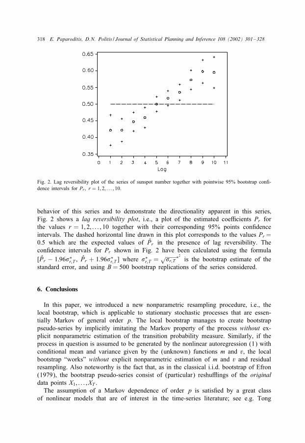
Fig. 2. Lag reversibility plot of the series of sunspot number together with pointwise 95% bootstrap con.-dence intervals for Pr; r = 1; 2; : : : ; 10.

behavior of this series and to demonstrate the directionality apparent in this series;Fig. 2 shows a lag reversibility plot, i.e., a plot of the estimated coeTcients Pr forthe values r = 1; 2; : : : ; 10 together with their corresponding 95% points con.denceintervals. The dashed horizontal line drawn in this plot corresponds to the values Pr =0:5 which are the expected values of Pr in the presence of lag reversibility. Thecon.dence intervals for Pr shown in Fig. 2 have been calculated using the formula[Pr − 1:96�∗

r;T ; Pr + 1:96�∗r;T ] where �∗

r;T =√�r;T

∗2

is the bootstrap estimate of thestandard error, and using B = 500 bootstrap replications of the series considered.

6. Conclusions

In this paper, we introduced a new nonparametric resampling procedure, i.e., thelocal bootstrap, which is applicable to stationary stochastic processes that are essen-tially Markov of general order p. The local bootstrap manages to create bootstrappseudo-series by implicitly imitating the Markov property of the process without ex-plicit nonparametric estimation of the transition probability measure. Similarly, if theprocess in question is assumed to be generated by the nonlinear autoregression (1) withconditional mean and variance given by the (unknown) functions m and v, the localbootstrap “works” without explicit nonparametric estimation of m and v and residualresampling. Also noteworthy is the fact that, as in the classical i.i.d. bootstrap of Efron(1979), the bootstrap pseudo-series consist of (particular) reshuOings of the originaldata points X1; : : : ; XT .

The assumption of a Markov dependence of order p is satis.ed by a great classof nonlinear models that are of interest in the time-series literature; see e.g. Tong


(1990). Thus, our procedure is potentially applicable to a large variety of statisticalinference problems in nonlinear time-series analysis. In this paper, we have focusedon some speci.c applications for which the asymptotic validity of the local bootstrapprocedure has been established. We have also presented a limited number of real dataand .nite-sample simulations indicating the performance of the local bootstrap in suchsituations.

Acknowledgements

The authors thank the editor and, referees and Michael Neumann for very helpfulcomments.

Appendix A. Proofs

Proof of Theorem 3.1. For X1; X2; : : : ; XT given; let B(ET ) be the �-.eld of all .nitesubsets of ET = X

pT where X

pT denotes the Cartesian product of p copies of XT ≡

{X1; X2; : : : ; XT}. Let =T =∏∞

k=1 Ek;T where Ek;T is a copy of ET equipped with a copyof the �-.eld B(ET ) and denote by AT the product �-.eld on =T . Consider now theMarkov chain Y∗ = {Y∗

t ; t¿ 1} on the path space (=T ;AT ; P∗�0

) de.ned as follows:For any A∈AT and for �0 an appropriate initial distribution; P∗

�0(Y∗ ∈A) describes the

probability of the event Y∗ ∈A when L(Y∗1 ) = �0. Apart from the initial distribution

�0; P∗�0

(·) is determined by the temporarily homogeneous transition probability kernelP(x; z) = P(Y∗

t+1 = z|Y∗t = x) which for Y∗

t = x and x = (x1; x2; : : : ; xp)∈ET is givenby

P(x; z) =

Wb(x−Yj)∑T−1m=p Wb(x−Ym)

if z = (Xj+1; x1; x2; : : : ; xp−1); p6 j6T − 1;

0 else:(A.1)

Now; verify that by (B1) for every b¿ 0; ET ⊂ ET with ET = XpT and XT =

{Xp+1; Xp+2; : : : ; XT} is an absorbing communicating class; i.e.;∑

z∈ETP(x; z) = 1 for

all x∈ET . Furthermore; by Theorem 2.3 of Doob (1953; p. 180); t0 ∈N exists such thatP(Y∗

t0 ∈ET |Y∗1 =x)=1 for all x∈ ET \ET . By Proposition 4.1.2 of Meyn and Tweedie

(1993; p. 84); it follows then that an irreducible Markov chain denoted by Y∗T exists

whose state space is restricted to ET and with transition probability matrix PET ; i.e.;the restriction of the matrix P = (P(x; z))x;z∈ET

to the absorbing and communicatingclass ET . The positive recurrence of the chain is a simple consequence of |ET |¡∞while the aperiodicity follows from (A.1) and the fact that by (B1); Wb(x − Yj)¿ 0for every b¿ 0 and p6 j6T − 1.

Since we are dealing in the sequel with the asymptotic properties of the local re-sampling procedure we ignore in what follows the eDects of the starting values andassume that the bootstrap chain Y∗

T starts with its stationary distribution (6), i.e., thatY∗

p ∼ �∗T .


Lemma 6.1. Under the assumptions of Theorem 3.2 we have for every y∈R;

supx∈S

∣∣∣∣∣ 1TT−1∑j=p

1(−∞;y](Xj+1)Wb(x− Yj) −∫

1(−∞;y](z)fXt+1Yt (z; x) dz

∣∣∣∣∣→ 0 a:s:

as T → ∞.

Proof. In the following we use the shorthand f(z; x) for fXt+1Yt (z; x). The result isestablished by showing that

supx∈S

|E[r∗b (x)] − r(x)| → 0 a:s: (A.2)

and

supx∈S

|r∗b (x) − E[r∗b (x)]| → 0 a:s:; (A.3)

where

r∗b (x) =1

T − p

T−1∑j=p

1(−∞;y](Xj+1)Wb(x− Yj)

and

r(x) =∫

1(−∞;y](z)f(z; x) dz:

Note that r∗b (x) is asymptotically equivalent to T−1∑T−1j=p 1(−∞;y](Xj+1)Wb(x − Yj).

For (A.2) we have

supx∈S

|E[r∗b (x)] − r(x)| = supx∈S

∣∣∣∣∫ y

−∞

∫(f(z; x− ub) − f(z; x))W (u) du dz

∣∣∣∣6 sup

x∈S

∫ ∣∣∣∣∫ y

−∞(f(z; x− ub) − f(z; x)) dz

∣∣∣∣W (u) du

= b L(y)∫

‖u‖W (u) du

= O(b);

where the last inequality follows using (A.2)(ii) and (B1).To handle (A.3) we apply the technique of splitting the supremum over x∈S. Since

S is compact it can be covered by a .nite number NT of cubes Ii;T with centers xi

the sides of which are of length LT . From (B1) and the mean value theorem we thenhave

supx∈S

|r∗b (x) − E[r∗b (x)]|

= max16i6NT

supx∈S∩Ii

∣∣∣∣∣ 1TT−1∑j=p

1(−∞;y](Xj+1)Wb(x− Yj)


−E[1(−∞;y](Xj+1)Wb(x− Yj)]|

6 max16i6NT

∣∣∣∣∣ 1TT−1∑j=p

Zj;T (xi)

∣∣∣∣∣+ C∗LTb−(p+1);

where C∗ ¿ 0 and

Zj;T (xi) = 1(−∞;y](Xj+1)Wb(xi − Yj) − E[1(−∞;y](Xj+1)Wb(xi − Yj)]:

Now, by (B1), |Zj;T (xi)|6Mb−p. For j¿ 0 arbitrary, let LT = jbp+1=2C∗ and notethat NT = O(L−p

T ). Applying inequality (1.4) of Roussas (1988, p. 136), we get

P

(max

16i6NT

∣∣∣∣∣ 1TT∑

j=p

Zj;T (xi)

∣∣∣∣∣¿ j2

)6NT max

16i6NT

P

(1T

∣∣∣∣∣T−1∑j=p

Zj;T (xi)

∣∣∣∣∣¿ j2

)

6O(L−pT )C T−l=2+l#p

for any l¿ 2 such that∑∞

j=1 (j + 1)l=2−1�(j)¡∞, where �(·) is the (strong) mixing

coeTcient of {Xt; t¿ 1} and C ¿ 0. Now, by the above choice of LT we get that inorder for the Borel–Cantelli Lemma to apply, the condition l=2− l#p− #p(p+ 1)¿ 1should be satis.ed, i.e.,

0¡#¡l

2lp + 2p(p + 1)− 1

lp + p(p + 1):

Finally, 0¡#¡ 1=2p follows because by the exponential decrease of the strong mixingcoeTcient �(j) we have

∑∞j=1 (j + 1)l=2−1�(j)¡∞ for every l¿ 2.

For x∈S, let

f∗b (x) =

1T

T−1∑j=p

Wb(x− Yj):

Setting y = ∞ in the proof of the above lemma we immediately get supx∈S |f∗b (x) −

f(x)| → 0 a.s.; cf. also Theorem 3.2 of Roussas (1988).

Proof of Theorem 3.2. It suTces to show the strong uniform convergence of F∗T (y|x)

to F(y|x) over S for every y∈R. The asserted uniform convergence over y∈R followsthen by the same arguments as in the proof of the Glivenko–Cantelli Theorem; cf. alsothe proof of Theorem 3.1 in Roussas (1969; p. 1390). Now; since

|F∗T (y|x) − F(y|x)|6 1

f∗b (x)

{|r∗b (x) − r(x)| + F(y|x)|f∗b (x) − f(x)|};

the result follows by (A.3) and Lemma 6.1.

Proof of Theorem 3.3. As in the proof of Theorem 3.2 it suTces to show the strongconvergence of F∗

T (y) to F(y) for every y∈R. Now; for almost all sample paths{Xt; t¿ 1} we have by Theorem 3.2 that F∗

T (y|x) → F(y|x). So take any one of the


sample paths for which the above holds and consider the sequence of bootstrap sta-tionary distribution functions {F∗

Y;T (y)}T∈N corresponding to the sequence of bootstrapMarkov chains {Y∗

T}T=1;2; ::: where for y = (y1; y2; : : : ; yp) and x = (x1; x2; : : : ; xp);

F∗Y;T (y) =

∫F∗Y;T (y|x) dF∗

Y;T (x)

=∫ p∏

i=2

1(−∞;yi](xi−1)F∗T (y1|x) dF∗

Y;T (x):

By Helly’s selection theorem; Billingsley (1995; p. 336); a subsequence {F∗Y;Tk

(y)}k=1;2; :::

exists such that for all continuity points y∈Rp of G;

limk→∞

F∗Y;Tk

(y) = G(y);

where G is a right continuous; nondecreasing function satisfying 06G(y)6 1. Sinceby (A3) the sequence {F∗

Y;T (y)} is tight; G is also a distribution function. Let g : Rp →R be any bounded and continuous function and note .rst that limk→∞

∫g(y)dF∗

Y;Tk(y)

→ ∫g(y)dG(y). Using the notation yp−1 = (y1; y2; : : : ; yp−1) we further get∫

g(z; yp−1)dF∗Y;Tk

(z; yp−1) =∫

g(z; yp−1)F∗Tk

(dz|y)dF∗Y;Tk

(y)

=∫

g(z; yp−1)F(dz|y)dF∗Y;Tk

(y)

+∫

g(z; yp−1)(F∗Tk

(dz|y) − F(dz|y))dF∗Y;Tk

(y)

→∫

g(z; yp−1)F(dz|y)dG(y)

as k → ∞, where the last convergence follows by Theorem 3.2, the continuity ofg(y) =

∫g(z; yp−1)F(dz|y) and the weak convergence F∗

Y;Tk⇒G. Thus G is a stationary

distribution of Yt =(XtXt−1; : : : ; Xt−p+1) from which G=FY follows by the uniquenessof FY. Since the above is true for every subsequence {F∗

Y;Tk(y)} of {F∗

Y;T (y)} thatconverge at all; we conclude by a corollary in Billingsley (1995; p. 381); that

limT→∞

F∗Y;T (y) = FY(y): (A.4)

Since F∗Y;T (y) → FY(y) occurs for any sample path in a set of sample paths that has

probability one; we conclude that F∗T (y) → F(y) a.s.

Proof of Theorem 3.4. Consider the process {X+t } de.ned by X+

t =X ∗t +ut where {ut}

is an i.i.d. sequence of random variables having the uniform distribution U [− hT ; hT ).{ut} is assumed to be independent of {X ∗

t } while hT is some sequence depending onT such that hT → 0 as T → ∞ at some rate to be speci.ed later. Denote by -+

T


the --mixing coeTcient of {X+t }. By a theorem of Csaki and Fisher; cf. Theorem 3.1

in Bradley (1986); we have that -∗T = -+

T and therefore the assertion of the Theoremis established if we show the required --mixing property for the sequence {X+

t }. Infact more is true; i.e.; it can be shown that {X+

t } is uniformly ergodic from whichthe required exponential decrease of the -+-mixing coeTcient follows by Theorem1 of Doukhan (1994; p. 88). To see the uniform ergodicity of {X +

t } note .rst thatthe one-step transition distribution function of {X+

t }; denoted by F+T (y|x); is given

by F+T (y|x) =

∫Fu;T (y − z) dF∗

T (z|x) with Fu;T (·) the distribution function of ut . Theone-step transition density of {X+

t } is given by

f+T (y|x) =

12hT

T∑j=p+1

1(y−hT ;y+hT ](X ∗j )P(X ∗

t+1 = Xj|Y∗t = x)

=1

2hT[F∗

T (y + hT |x) − F∗T (y − hT |x)]:

Thus we have

supy∈R

supx∈S

|f+(y|x) − f(y|x)|

61

2hTsupy∈R

supx∈S

|F∗T (y + hT |x) − F(y + hT |x)|

+1

2hTsupy∈R

supx∈S

|F∗T (y − hT |x) − F(y − hT |x)|

+ supy∈R

supx∈S

∣∣∣∣ 12hT

{F(y + hT |x) − F(y − hT |x)} − f(y|x)∣∣∣∣

= S1 + S2 + S3:

Now; let hT ∼ (log(T ))−1 and verify that by the same arguments as in the proof ofLemma 6.1 and Theorem 3.2; S1 → 0 and S2 → 0 a.s. as T → ∞ and b → 0 suchthat (B2) is satis.ed. Furthermore; for S3 we get by the mean value theorem for somey¡y1 ¡y + hT and y − hT ¡y2 ¡y that

S3 = supy

supx∈S

∣∣∣∣12{f(y1|x) + f(y2|x)} − f(y|x)∣∣∣∣

612

supy

supx∈S

|f(y1|x) − f(y|x)| +12

supy

supx∈S

|f(y2|x) − f(y|x)|

= O(hT );

where the last inequality follows using the Lipschitz continuity in (A.2)(iii).To conclude the proof of the uniform ergodicity of {X+

t } we use Theorem 16.2.4of Meyn and Tweedie (1993) and show that a nonnegative measure < exists suchthat for Y+

t = (X+t ; X+

t−1; : : : ; X+t−p+1); P(Y+

t+p ∈A|Y+t = x)¿ <(A) for all x∈S. We


demonstrate this for the case p= 1 the general case being handled in exactly the samemanner. Thus let p = 1 and note that by (A.3), B¿ 0 exists such that f(·|x)¿ B¿ 0for all x∈ S. Furthermore, T0 ∈N exists such that supy supx |f+

T (y|x) − f(y|x)|¡B=2for all T¿T0. Hence,

P(X+t+1 ∈A|X+

t = x)¿∫Af(z|x) dz −

∫A|f+

T (z|x) − f(z|x)| dz

¿ BC(A) − B2C(A)

=B2C(A);

where C denotes Lebesgue measure.

Proof of Theorem 4.1. By the Markov property; Theorems 3.2 and 3.3 we have thatfor every .xed k ∈N and in a set of sample paths of {Xt; t¿ 1} that has probabilityone

F∗X ∗t ; X ∗

t+1 ;:::; X∗t+k+m−1

⇒ FXt ;Xt+1 ;:::; Xt+k+m−1 (A.5)

in the weak sense as T → ∞. Here F∗X ∗t ; X ∗

t+1 ;:::; X∗t+k+m−1

denotes the joint distributionfunction of X ∗

t ; X∗t+1; : : : ; X

∗t+k+m−1 while FXt ;Xt+1 ;:::; Xt+k+m−1 the joint distribution function

of Xt; Xt+1; : : : ; Xt+k+m−1. From this and by the continuity of g and the de.nition of Zt;(resp. Z∗

t ); we have with probability one;

F∗Z∗t ; Z∗

t+1 ;:::; Z∗t+k

⇒ FZt ; Zt+1 ;:::;; Zt+k : (A.6)

Furthermore; recall that by (A3) X ∗t takes its values in the compact set S. This fact;

together with the continuity of g; implies that the sequences |Z∗t |2 and |Z∗

t Z∗t+h| are

uniformly integrable. Therefore; using (A.6) we get for every integer h; 16 h6 kthat

E∗|Z∗t |2 → E|Zt |2 a:s: (A.7)

and

E∗(Z∗t Z

∗t+h) → E(ZtZt+h) a:s: (A.8)

Now, to prove the .rst part of the theorem, note that for B¿ 0 arbitrary, k1=k1(B)∈Nexists such that

2∞∑

5=k1+1

|Cov(Z1; Z1+5)|¡B=3: (A.9)

Furthermore, for %∈ (0; 1) as in Theorem 3.4, k2 = k2(B)∈N exists such that

2%k2+1

1 − %¡

B6 Var(Zt)

: (A.10)


Let k = max{k1; k2}. We then have

|�∗2

g;T − �2g|6

∣∣∣∣∣Var∗(Z∗1 ) − Var(Z1) + 2

k∑5=1

(Cov∗(Z∗1 ; Z

∗1+5) − Cov(Z1; Z1+5))

∣∣∣∣∣+ 2

T−1∑5=k+1

|Cov∗(Z∗1 ; Z

∗1+5)| + 2

∞∑5=k+1

|Cov(Z1; Z1+5)|: (A.11)

Because of (A.7) and (A.8), T1 ∈N exists such that

|Var∗(Z∗1 ) − Var(Z1)| + 2

k∑5=1

|Cov∗(Z∗1 ; Z

∗1+5) − Cov(Z1; Z1+5)|¡B=3: (A.12)

Furthermore, T2 ∈N exists such that

|Var∗(Z∗1 ) − Var(Z1)|¡ B(1 − %)

12%k+1 : (A.13)

Now, let T ∗ = max{T0; T1; T2} where T0 is given in Theorem 3.4. For T¿T ∗ wethen have using (A.10) and (A.13) and the inequality for --mixing sequences givenin Theorem 3 of Doukhan (1994, p. 9) that

2T−1∑

5=k+1

|Cov∗(Z∗1 ; Z

∗1+5)|

6 2T−1∑

5=k+1

%5 Var∗(Z∗1 )

62%k+1

1 − %Var(Z1) +

2%k+1

1 − %|Var∗(Z∗

1 ) − Var(Z1)|¡B=3: (A.14)

Thus from (A.11) and using (A.9), (A.12) and (A.11) we conclude that |�∗2

g;T −�2g|¡B.

To prove the second part of the theorem note .rst that by (A3) and (A.6) we havefor some 4¿ 0 that E∗|Z∗

t |2+4 → E|Zt |2+4 a.s. Now, since --mixing implies �-mixing,the assertion follows by Theorems 3.4 and 1.7 of Ibragimov (1962).

Proof of Theorem 4.2. The proof of weak convergence follows from Theorem 4.1 bymeans of the Cramer–Wold Device; cf. Brockwell and Davis (1991). Convergence ofsecond moments follows from weak convergence and Theorem (viii-B) of Rao (1973;p. 121).

Proof of Proposition 4.1. Assertion (1) of the proposition follows by the same ar-guments as in the proof of the .rst part of Theorem 4.1. Part (2) is an immedi-ate consequence of the fact that 06 I∗t; r6 1; Theorems 3.4 and 1.6 of Ibragimov(1962).


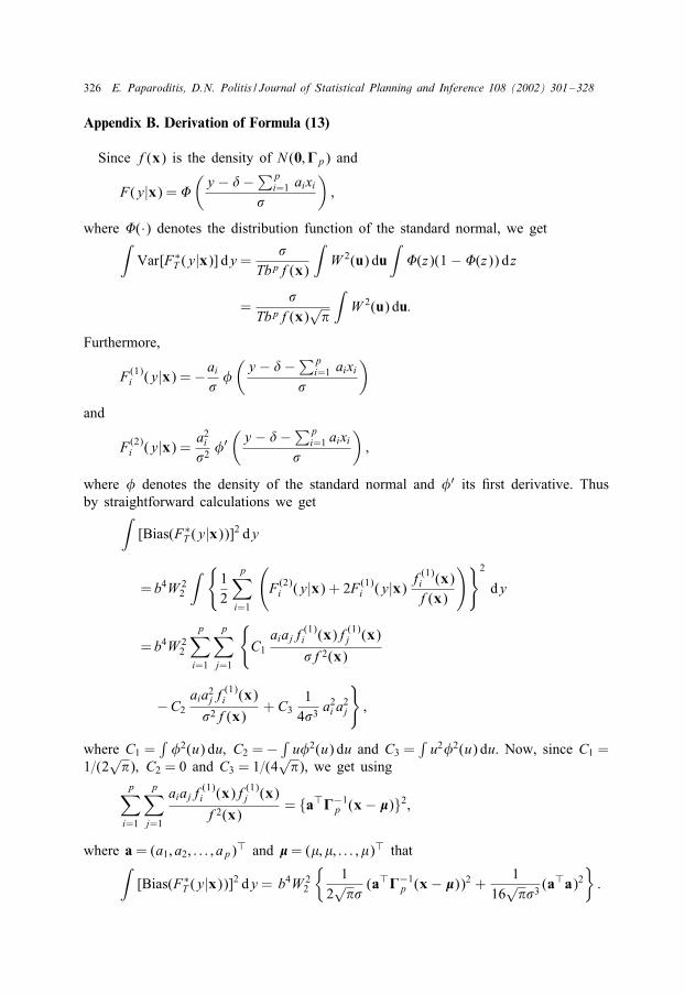
Appendix B. Derivation of Formula (13)

Since f(x) is the density of N (0;&p) and

F(y|x) = D(y − #−∑p

i=1 aixi�

);

where D(·) denotes the distribution function of the standard normal, we get∫Var[F∗

T (y|x)] dy =�

Tbpf(x)

∫W 2(u) du

∫D(z)(1 − D(z)) dz

=�

Tbpf(x)√�

∫W 2(u) du:

Furthermore,

F (1)i (y|x) = −ai

�E(y − #−∑p

i=1 aixi�

)

and

F (2)i (y|x) =

a2i

�2 E′(y − #−∑p

i=1 aixi�

);

where E denotes the density of the standard normal and E′ its .rst derivative. Thusby straightforward calculations we get∫

[Bias(F∗T (y|x))]2 dy

= b4W 22

∫ {12

p∑i=1

(F (2)i (y|x) + 2F (1)

i (y|x)f(1)i (x)f(x)

)}2

dy

= b4W 22

p∑i=1

p∑j=1

{C1

aiajf(1)i (x)f(1)

j (x)

�f2(x)

−C2aia2

jf(1)i (x)

�2f(x)+ C3

14�3 a2

i a2j

};

where C1 =∫E2(u) du; C2 = − ∫ uE2(u) du and C3 =

∫u2E2(u) du. Now, since C1 =

1=(2√�); C2 = 0 and C3 = 1=(4

√�), we get using

p∑i=1

p∑j=1

aiajf(1)i (x)f(1)

j (x)

f2(x)= {a�&−1

p (x− �)}2;

where a = (a1; a2; : : : ; ap)� and � = (<; <; : : : ; <)� that∫[Bias(F∗

T (y|x))]2 dy = b4W 22

{1

2√��

(a�&−1p (x− �))2 +

116√��3 (a�a)2

}:


References

Ango Nze, P., 1992. CritZeries d’ ergodicit[e de quelques modZeles Za repr[esentation markoviene. C. R. Acad.Sci. Paris 315 (1), 1301–1304.

Auestad, B., TjHstheim, D., 1990. Identi.cation of nonlinear time series: .rst order characterization and orderdetermination. Biometrika 77, 669–687.

Auestad, B., TjHstheim, D., 1991. Functional identi.cation in nonlinear time series. In: Roussas, G. (Ed.),Nonparametric Functional Estimation and Related Topics. Kluwer Academic Publishers, Dordrecht.

Billingsley, P., 1995. Probability and Measure. Wiley, New York.Bradley, R.C., 1986. Basic properties of strong mixing conditions. In: Eberlein, E., Taqqu, M.S. (Eds.),

Dependence in Probability and Statistics. Brikhauser, Boston, MA, pp. 165–192.Brockwell, P.J., Davis, R.A., 1991. Time Series: Theory and Methods, 2nd Edition. Springer, Berlin.Chan, K.S., Tong, H., Stenseth, N.C., 1997. Analyzing short time series data from periodically ]uctuating

rodent populations by threshold models: a nearest block bootstrap approach. Technical Report, No. 258,Department of Statistics and Actuarial Science, University of Iowa.

Chen, R., Tsay, R.S., 1993. Nonlinear additive ARX models. J. Amer. Statist. Assoc. 88, 955–967.Doob, J.L., 1953. Stochastic Processes. Wiley, New York.Doukhan, P., 1994. Mixing. Properties and Examples. . Lecture Notes in Statistics, Vol. 85. Springer, New

York.Efron, B., 1979. Bootstrap methods: another look at the jackknife. Ann. Statist. 7, 1–26.Efron, B., Tibshirani, R., 1986. Bootstrap measures for standard errors, con.dence intervals, and other

measures of statistical accuracy. Statist. Sci. 1, 54–77.Efron, B., Tibshirani, R., 1993. An Introduction to the Bootstrap. Chapman & Hall, New York.Falk, M., Reiss, R.-D., 1992. Bootstrapping conditional curves. In: JJockel, K.H., Rothe, G., Sendler, W.

(Eds.), Bootstrapping and Related Techniques, Lecture Notes in Economics and Mathematical Systems,Vol. 376. Springer, New York.

Fan, J., Gijbels, I., 1996. Local Polynomial Modelling and its Applications. Chapman & Hall, New York.Franke, J., HJardle, W., 1992. On bootstrapping kernel spectral estimates. Ann. Statist. 20, 121–145.Franke, J., Kreiss, J.-P., Mammen, E., 1996. Bootstrap of kernel smoothing in nonlinear time series, preprint.Freedman, D.A., 1984. On bootstrapping two-stage least-squares estimates in stationary linear models. Ann.

Statist. 12, 827–842.HJardle, W., Vieu, P., 1992. Kernel regression smoothing of time series. J. Time Series Anal. 13, 209–232.Ibragimov, I.A., 1962. Some limit theorems for stationary processes. Theory Probab. and Appl. 7, 349–382.Kim, T.Y., Cox, D., 1996. Bandwidth selection in kernel smoothing of time series. J. Time Series Anal. 17,

49–63.KJunsch, H., 1989. The jackknife and the bootstrap for general stationary observations. Ann. Statist. 17,

1217–1241.Lall, U., Sharman, A., 1996. A nearest neighbor bootstrap for resampling hydrologic time series. Water

Resources Res. 32, 679–693.Lawrence, A.J., 1991. Directionality and reversibility in time series. Int. Statist. Rev. 59, 67–79.Liu, R.Y., Singh, K., 1992. Moving blocks jackknife and bootstrap capture weak dependence. In: R. LePage,

L. Billard (Eds.), Exploring the Limits of the Bootstrap. Wiley, New York, pp. 225–248.Meyn, S.P., Tweedie, R.L., 1993. Markov Chains and Stochastic Stability. Springer, London.Politis, D.N., Romano, J.P., 1992. A general resampling scheme for triangular arrays of �-mixing random

variables with application to the problem of spectral density estimation. Ann. Statist. 20, 1985–2007.Politis, D.N., Romano, J.P., 1994. The stationary bootstrap. J. Amer. Statist. Assoc. 89, 1303–1313.Rajarshi, M.B., 1990. Bootstrap in Markov-sequences based on estimates of transition density. Ann. Institut.

Statist. Math. 42, 253–268.Rao, C.R., 1973. Linear Statistical Inference and its Applications, 2nd Edition. Wiley, New York.Roussas, G.G., 1969. Nonparametric estimation of the transition distribution function of a Markov process.

Ann. Statist. 40, 1386–1400.Roussas, G.G., 1988. Nonparametric estimation in mixing sequences of random variables. J. Statist. Plann.

Infer. 18, 135–149.Shao, J., Tu, D., 1995. The Jackknife and the Bootstrap. Springer, New York.


Shi, S.G., 1991. Local Bootstrap. Ann. Institut. Statist. Math. 43, 667–676.Tong, H., 1990. Nonlinear Time Series: A Dynamical Approach. Oxford University Press, New York.TjHstheim, D., 1990. Nonlinear time series and Markov chains. Adv. in Appl. Probab. 22, 587–611.TjHstheim, D., 1994. Nonlinear time series: a selective review. Scandinavian J. Statist. 21, 97–130.TjHstheim, D., Auestad, B., 1994. Nonparametric identi.cation of nonlinear time series: selecting signi.cant

lags. J. Amer. Statist. Assoc. 89, 1410–1419.Tsay, R., 1992. Model checking via parametric bootstraps in time series analysis. Appl. Statist. 41, 1–15.Weiss, G., 1975. Time reversibility of linear stochastic processes. J. Appl. Probab. 12, 831–836.

the local bootstrap for markov processesbhansen/718/paparoditispolitisnp.pdfblocks-of-blocks...

Documents