the interpolation theory of radial basis functions. - cato
TRANSCRIPT
THE INTERPOLATION THEORY
OF RADIAL BASIS FUNCTIONS
by
Bradley John Charles Baxter
of
Trinity College
A dissertation presented in fulfilment of the requirements for
the degree of Doctor of Philosophy, Cambridge University
August 1992
i

THE INTERPOLATION THEORY
OF RADIAL BASIS FUNCTIONS
B. J. C. Baxter
Summary
The problem of interpolating functions of d real variables (d > 1) occurs naturally
in many areas of applied mathematics and the sciences. Radial basis function
methods can provide interpolants to function values given at irregularly positioned
points for any value of d. Further, these interpolants are often excellent approxi-
mations to the underlying function, even when the number of interpolation points
is small.
In this dissertation we begin with the existence theory of radial basis function
interpolants. It is first shown that, when the radial basis function is a p-norm
and 1 < p < 2, interpolation is always possible when the points are all different
and there are at least two of them. Our approach extends the analysis of the case
p = 2 devised in the 1930s by Schoenberg. We then show that interpolation is not
always possible when p > 2. Specifically, for every p > 2, we construct a set of
different points in some Rd for which the interpolation matrix is singular. This
construction seems to have no precursor in the literature.
The greater part of this work investigates the sensitivity of radial basis func-
tion interpolants to changes in the function values at the interpolation points.
This study was motivated by the observation that large condition numbers occur
in some practical calculations. Our early results show that it is possible to recast
the work of Ball, Narcowich and Ward in the language of distributional Fourier
transforms in an elegant way. We then use this language to study the interpola-
tion matrices generated by subsets of regular grids. In particular, we are able to
extend the classical theory of Toeplitz operators to calculate sharp bounds on the
spectra of such matrices. Moreover, we also describe some joint work with Charles
Micchelli in which we use the theory of Polya frequency functions to continue this
work, as well as shedding new light on some of our earlier results.
ii

Applying our understanding of these spectra, we construct preconditioners for
the conjugate gradient solution of the interpolation equations. The preconditioned
conjugate gradient algorithm was first suggested for this problem by Dyn, Levin
and Rippa in 1983, who were motivated by the variational theory of the thin
plate spline. In contrast, our approach is intimately connected to the theory of
Toeplitz forms. Our main result is that the number of steps required to achieve
solution of the linear system to within a required tolerance can be independent of
the number of interpolation points. In other words, the number of floating point
operations needed for a regular grid is proportional to the cost of a matrix-vector
multiplication. The Toeplitz structure allows us to use fast Fourier transform
techniques, which implies that the total number of operations is a multiple of
n log n, where n is the number of interpolation points.
Finally, we use some of our methods to study the behaviour of the multiquadric
when its shape parameter increases to infinity. We find a surprising link with
the sinus cardinalis or sinc function of Whittaker. Consequently, it can be highly
useful to use a large shape parameter when approximating band-limited functions.
iii

Declaration
In this dissertation, all of the work is my own with the exception of Chapter 5,
which contains some results of my collaboration with Dr Charles Micchelli of the
IBM Research Center, Yorktown Heights, New York, USA. This collaboration was
approved by the Board of Graduate Studies.
No part of this thesis has been submitted for a degree elsewhere. However,
the contents of several chapters have appeared, or are to appear, in journals. In
particular, we refer the reader to Baxter (1991a, b, c) and Baxter (1992a, b).
Furthermore, Chapter 2 formed a Smith’s Prize essay in an earlier incarnation.
iv

Preface
It is a pleasure to acknowledge the support I have received during my doctoral
research.
First, I must record my gratitude to Professor Michael Powell for his sup-
port, patience and understanding whilst supervising my studies. His enthusiasm,
insight, precision, and distrust for gratuitous abstraction have enormously influ-
enced my development as a mathematician. In spite of his many commitments he
has always been generous with his time. In particular, I am certain that the great
care he has exhibited when reading my work will be of lasting benefit; there could
be no better training for the preparation and refereeing of technical papers.
The Numerical Analysis Group of the University of Cambridge has provided
an excellent milieu for research, but I am especially grateful to Arieh Iserles, whose
encouragement and breadth of mathematical knowledge have been of great help
to me. In particular, it was Arieh who introduced me to the beautiful theory of
Toeplitz operators.
Several institutions have supported me financially. The Science and Engineer-
ing Research Council and A.E.R.E. Harwell provided me with a CASE Research
Studentship during my first three years. At this point, I must thank Nick Gould
for his help at Harwell. Subsequently I have been aided by Barrodale Computing
Limited, the Amoco Research Company, Trinity College, Cambridge, and the en-
dowment of the John Humphrey Plummer Chair in Applied Numerical Analysis,
for which I am once more indebted to Professor Powell. Furthermore, these in-
stitutions and the Department of Applied Mathematics and Theoretical Physics,
have enabled me to attend conferences and enjoy the opportunity to work with
colleagues abroad. I would also like to thank David Broomhead, Alfred Cavaretta,
Nira Dyn, David Levin, Charles Micchelli, John Scales and Joe Ward, who have
invited and sponsored my visits, and have invariably provided hospitality and
kindness.
There are many unmentioned people to whom I owe thanks. Certainly this
work would not have been possible without the help of my friends and family. In
v

particular, I thank my partner, Glennis Starling, and my father. I am unable to
thank my mother, who died during the last weeks of this work, and I have felt this
loss keenly. This dissertation is dedicated to the memories of both my mother and
my grandfather, Charles S. Wilkins.
vi

Table of Contents
Chapter 1 : Introduction
1.1 Polynomial interpolation . . . . . . . . . . . . . . . . . . . . . . . . . . . . . . . . . . . . . . . . . page 3
1.2 Tensor product methods . . . . . . . . . . . . . . . . . . . . . . . . . . . . . . . . . . . . . . . . . page 4
1.3 Multivariate splines . . . . . . . . . . . . . . . . . . . . . . . . . . . . . . . . . . . . . . . . . . . . . . page 4
1.4 Finite element methods . . . . . . . . . . . . . . . . . . . . . . . . . . . . . . . . . . . . . . . . . . page 5
1.5 Radial basis functions . . . . . . . . . . . . . . . . . . . . . . . . . . . . . . . . . . . . . . . . . . . . page 6
1.6 Contents of the thesis . . . . . . . . . . . . . . . . . . . . . . . . . . . . . . . . . . . . . . . . . . . page 10
1.7 Notation . . . . . . . . . . . . . . . . . . . . . . . . . . . . . . . . . . . . . . . . . . . . . . . . . . . . . . . .page 12
Chapter 2 : Conditionally positive definite functions and p-norm distance
matrices
2.1 Introduction . . . . . . . . . . . . . . . . . . . . . . . . . . . . . . . . . . . . . . . . . . . . . . . . . . . . page 14
2.2 Almost negative matrices . . . . . . . . . . . . . . . . . . . . . . . . . . . . . . . . . . . . . . . page 15
2.3 Applications . . . . . . . . . . . . . . . . . . . . . . . . . . . . . . . . . . . . . . . . . . . . . . . . . . . . page 18
2.4 The case p > 2 . . . . . . . . . . . . . . . . . . . . . . . . . . . . . . . . . . . . . . . . . . . . . . . . . .page 25
Chapter 3 : Norm estimates for distance matrices
3.1 Introduction . . . . . . . . . . . . . . . . . . . . . . . . . . . . . . . . . . . . . . . . . . . . . . . . . . . . page 31
3.2 The univariate case for the Euclidean norm . . . . . . . . . . . . . . . . . . . . . .page 31
3.3 The multivariate case for the Euclidean norm . . . . . . . . . . . . . . . . . . . .page 35
3.4 Fourier transforms and Bessel transforms . . . . . . . . . . . . . . . . . . . . . . . .page 37
3.5 The least upper bound for subsets of a grid . . . . . . . . . . . . . . . . . . . . . .page 40
Chapter 4 : Norm estimates for Toeplitz distance matrices I
4.1 Introduction . . . . . . . . . . . . . . . . . . . . . . . . . . . . . . . . . . . . . . . . . . . . . . . . . . . . page 42
4.2 Toeplitz forms and Theta functions . . . . . . . . . . . . . . . . . . . . . . . . . . . . . .page 44
4.3 Conditionally negative definite functions of order 1 . . . . . . . . . . . . . . page 50
4.4 Applications . . . . . . . . . . . . . . . . . . . . . . . . . . . . . . . . . . . . . . . . . . . . . . . . . . . . page 58
vii

4.5 A stability estimate . . . . . . . . . . . . . . . . . . . . . . . . . . . . . . . . . . . . . . . . . . . . . page 62
4.6 Scaling the infinite grid . . . . . . . . . . . . . . . . . . . . . . . . . . . . . . . . . . . . . . . . . page 65
Appendix . . . . . . . . . . . . . . . . . . . . . . . . . . . . . . . . . . . . . . . . . . . . . . . . . . . . . . . page 68
Chapter 5 : Norm estimates for Toeplitz distance matrices II
5.1 Introduction . . . . . . . . . . . . . . . . . . . . . . . . . . . . . . . . . . . . . . . . . . . . . . . . . . . . page 70
5.2 Preliminary facts . . . . . . . . . . . . . . . . . . . . . . . . . . . . . . . . . . . . . . . . . . . . . . . .page 71
5.3 Polya frequency functions . . . . . . . . . . . . . . . . . . . . . . . . . . . . . . . . . . . . . . . page 80
5.4 Lower bounds on eigenvalues . . . . . . . . . . . . . . . . . . . . . . . . . . . . . . . . . . . . page 88
5.5 Total positivity and the Gaussian cardinal function . . . . . . . . . . . . . . page 92
Chapter 6 : Norm estimates and preconditioned conjugate gradients
6.1 Introduction . . . . . . . . . . . . . . . . . . . . . . . . . . . . . . . . . . . . . . . . . . . . . . . . . . . . page 95
6.2 The Gaussian . . . . . . . . . . . . . . . . . . . . . . . . . . . . . . . . . . . . . . . . . . . . . . . . . . . page 96
6.3 The multiquadric . . . . . . . . . . . . . . . . . . . . . . . . . . . . . . . . . . . . . . . . . . . . . . page 102
Chapter 7 : On the asymptotic cardinal function for the multiquadric
7.1 Introduction . . . . . . . . . . . . . . . . . . . . . . . . . . . . . . . . . . . . . . . . . . . . . . . . . . . page 118
7.2 Some properties of the multiquadric . . . . . . . . . . . . . . . . . . . . . . . . . . . .page 119
7.3 Multiquadrics and entire functions of exponential type π . . . . . . . page 121
7.4 Discussion . . . . . . . . . . . . . . . . . . . . . . . . . . . . . . . . . . . . . . . . . . . . . . . . . . . . . page 125
Chapter 8 : Conclusions . . . . . . . . . . . . . . . . . . . . . . . . . . . . . . . . . . . . . . . . . . . . page 126
References . . . . . . . . . . . . . . . . . . . . . . . . . . . . . . . . . . . . . . . . . . . . . . . . . . . . . . . . . . . .page 128
viii
1 : Introduction
The multivariate interpolation problem occurs frequently in many branches of
science and engineering. Typically, we are given a discrete set I in Rd, where d is
greater than one, and real numbers fii∈I . Our task is to construct a continuous
or sufficiently differentiable function s:Rd → R such that
s(i) = fi, i ∈ I, (1.1)
and we say that s interpolates the data (i, fi) : i ∈ I. Interpolants can be highly
useful. For example, we may need to approximate a function whose values are
known only at the interpolation points, that is we are ignorant of its behaviour
outside I. Alternatively, the underlying function might be far too expensive to
evaluate at a large number of points, in which case the aim is to choose an in-
terpolant which is cheap to compute. We can then use our interpolant in other
algorithms in order to, for example, calculate approximations to extremal values of
the original function. Another application is data-compression, where the size of
our initial data (i, fi) : i ∈ I exceeds the storage capacity of available computer
hardware. In this case, we can choose a subset I of I and use the corresponding
data to construct an interpolant with which we estimate the remaining values. It
is important to note that in general I will consist of scattered points, that is its
elements can be irregularly positioned. Thus algorithms that apply to arbitrary
distributions of points are necessary. Such algorithms exist and are well under-
stood in the univariate case (see, for instance, Powell (1981)), but many difficulties
intrude when d is bigger than one.
There are many applications of multivariate interpolation, but we prefer to
treat a particular application in some detail rather than provide a list. Therefore
we consider the following interesting example of Barrodale et al (1991).
When a time-dependent system is under observation, it is often necessary
to relate pictures of the system taken at different times. For example, when
measuring the growth of a tumour in a patient, we must expect many changes to
occur between successive X-ray photographs, such as the position of the patient
1

Introduction
or the amount of fluid in the body’s tissues. If we can identify corresponding
points on the two photographs, such as parts of the bone structure or intersections
of particular veins, then these pairs of points can be viewed as the data for two
interpolation problems. Specifically, let (xj , yj)nj=1 be the coordinates of the points
in one picture, and let the corresponding points in the second picture be (ξj , ηj)nj=1.
We need functions sx:R2 → R and sy:R2 → R such that
sx(xj , yj) = ξj and sy(xj , yj) = ηj for j = 1, . . . , n. (1.2)
Therefore we see that the scattered data interpolation problem arises quite nat-
urally as an attempt to approximate the non-linear coordinate transformation
mapping one picture into the next.
It is important to understand that interpolation is not always desirable. For
example, our data may be corrupted by measurement errors, in which case there
is no good reason to choose an approximation which satisfies the interpolation
equations, but we do want to construct an approximation which is close to the
function values in some sense. One option is to choose our function s:Rd → Rfrom some family (usually a linear space) of functions so as to minimize a certain
functional G, such as
G(s − f) =∑
i∈I
[fi − s(i)]2, (1.3)
which is the familiar least-squares fitting problem. Of course this can require
the solution of a nonlinearly constrained optimization problem, depending on the
family of functions and the functional G. Another alternative to interpolation
takes s to be the sum of decaying functions, each centred at a point in I and
taking the function value at that point. Such an approximation is usually called
a quasi-interpolant, reflecting the requirement that it should resemble the inter-
polant in some suitable way. These methods are of both practical and theoretical
importance, but we emphasize that this dissertation is restricted to interpolation,
specifically interpolation using radial basis functions, for which we refer the reader
to Section 1.5 and the later chapters of the dissertation.
2

Introduction
We now briefly describe some other multivariate approximation schemes. Of
course, our treatment does not provide a thorough overview of the field, for which
we refer the reader to de Boor (1987), Franke (1987) or Hayes (1987). However,
it is interesting to contrast radial basis functions with some of the other methods.
In fact, the memoir of Franke (1982) is dedicated to this purpose; it contains
careful numerical experiments using some thirty methods, including radial basis
functions, and provides an excellent reason for their theoretical study: they obtain
excellent accuracy when interpolating scattered data. Indeed, Franke found them
to excel in this sense when compared to the other tested methods, thus providing
an excellent reason for their theoretical study.
1.1 Polynomial interpolation
Let P be a linear space of polynomials in d real variables spanned by (pi)i∈I , where
I is the discrete subset of Rd discussed at the beginning of the introduction. Then
an interpolant s:Rd → R of the form
s(x) =∑
i∈I
cipi(x), x ∈ Rd, (1.4)
exists if and only if the matrix (pi(j))i,j∈I is invertible. We see that this prop-
erty depends on the geometry of the centres when d > 1, which is a signifi-
cant difficulty. One solution is to choose a particular geometry. As an example
we describe the tensor product approach on a “tartan grid”. Specifically, let
I = (xj , yk) : 1 ≤ j ≤ l, 1 ≤ k ≤ m, where x1 < · · · < xl and y1 < · · · < ym
are given real numbers, and let f(xj ,yk) : 1 ≤ j ≤ l, 1 ≤ k ≤ m be the func-
tion values at these centres. We let (L1j )
lj=1 and (L2
k)mk=1 be the usual univariate
Lagrange interpolating polynomials associated with the numbers (xj)l1 and (yk)m
1
respectively and define our interpolant s:R2 → R by the equation
s(x, y) =
l∑
j=1
m∑
k=1
f(xj ,yk)L1j (x)L2
k(y), (x, y) ∈ R2. (1.5)
Clearly this approach extends to any number of dimensions d.
3

Introduction
1.2 Tensor product methods
The tensor product scheme for tartan grids described in the previous section is
not restricted to polynomials. Using the same notation as before, we replace
(L1j )
lj=1 and (L2
k)mk=1 by univariate functions (Pj)
lj=1 and (Qk)m
k=1 respectively.
Our interpolant takes the form
s(x, y) =
l∑
j=1
m∑
k=1
yjkPj(x)Qk(y), (x, y) ∈ R2, (1.7)
from which we obtain the coefficients (yjk). By adding points outside the interval
[x1, xl] and [y1, ym] we can choose (Pj) and (Qk) to be univariate B-splines. In this
case the linear systems involved are invertible and banded, so that the number of
operations and the storage required are both multiples of the total number of points
in the tartan grid. Such methods are extremely important for the subtabulation
of functions on regular grids, and clearly the scheme exists for any number of
dimensions d. A useful survey is the book of Light and Cheney (1986)
1.3 Multivariate Splines
Generalizing some of the properties of univariate splines to a multivariate set-
ting has been an idee fixe of approximation theory. Thus the name “spline” is
overused, being applied to almost any extension of univariate spline theory. In this
section we briefly consider box splines. These are compactly supported piecewise
polynomial functions which extend Schoenberg’s characterization of the B-spline
B(·; t0, . . . , tk) with arbitrary knots t0, . . . , tk as the “shadow” of a k-dimensional
simplex (Schoenberg (1973), Theorem 1, Lecture 1). Specifically, the box spline
B(·;A) associated with the d × n matrix A is the distibution defined by
B(·;A) : C∞0 (Rd) → R : ϕ 7→
∫
[−1/2,1/2]nϕ(Ax) dx,
where C∞0 (Rd) is the vector subspace of C∞(Rd) whose elements vanish at infinity.
If we let a1, . . . , an ∈ Rd be the columns of A, then the Fourier transform of the
4

Introduction
box spline is given by
B(ξ;A) =
n∏
j=1
sinc ξT aj , ξ ∈ Rd,
where sinc(x) = sin(x/2)/(x/2). We see that a simple example of a box spline
is a tensor product of univariate B-splines. It can be shown that there exist box
splines with smaller supports than tensor product B-splines.
A large body of mathematics now exists, and a suitable comprehensive
review is the long paper of Dahmen and Micchelli (1983). Further, this theory is
also yielding useful results in the study of wavelets (see Chui (1992)). However,
there are many computational difficulties. At present, box spline software is not
available from the main providers of scientific computation packages.
1.4 Finite element methods
Finite element methods can provide extremely flexible piecewise polynomial spaces
for approximation and scattered data interpolation. When d = 2 we first choose
a triangulation of the points. Then a polynomial is constructed on each triangle,
possibly using function values and partial derivative values at other points in
addition to the vertices of the triangulation. This is a non-trivial problem, since
we usually require some global differentiability properties, that is the polynomials
must fit together in a suitably smooth way. Further, the partial derivatives are
frequently unknown, and these methods can be highly sensitive to the accuracy of
their estimates (Franke (1982)).
Much recent research has been directed towards the choice of triangula-
tion. The Delaunay triangulation (Lawson (1977)) is often recommended, but
some work of Dyn, Levin and Rippa (1986) indicates that greater accuracy can be
achieved using data-dependent triangulations, that is triangulations whose com-
ponent triangles reflect the geometry of the function in some way. Finally, the
complexity of constructing triangulations in higher dimensions effectively limits
these methods to two and three dimensional problems.
5

Introduction
1.5 Radial basis functions
A radial basis function approximation takes the form
s(x) =∑
i∈I
yiϕ(‖x − i‖), x ∈ Rd, (1.8)
where ϕ: [0,∞) → R is a fixed univariate function and the coefficients (yi)i∈I
are real numbers. We do not place any restriction on the norm ‖ · ‖ at this
point, although we note that the Euclidean norm is the most common choice.
Therefore our approximation s is a linear combination of translates of a fixed
function x 7→ ϕ(‖x‖) which is “radially symmetric” with respect to the given
norm, in the sense that it clearly possesses the symmetries of the unit ball. We
shall often say that the points (xj)nj=1 are the centres of the radial basis function
interpolant. Moreover, it is usual to refer to ϕ as the radial basis function, if the
norm is understood.
If I is a finite set, say I = (xj)nj=1, the interpolation conditions provide the
linear system
Ay = f, (1.9)
where
A =(ϕ(‖xj − xk‖)
)n
j,k=1, (1.10)
y = (yj)nj=1 and f = (fj)
nj=1.
One of the most attractive features of radial basis function methods is the
fact that a unique interpolant is often guaranteed under rather mild conditions
on the centres. In several important cases, the only restrictions are that there
are at least two centres and they are all distinct, which are as simple as one
could wish. However, one important exception to this statement is the thin plate
spline introduced by Duchon (1975, 1976), where we choose ϕ(r) = r2 log r. It
is easy to see that the interpolation matrix A given by (1.10) can be singular for
non-trivial sets of distinct centres. For example, choosing x2, . . . , xn to be any
different points on the sphere of unit radius whose centre is x1, we conclude that
the first row and column of A consist entirely of zeros. Of course, such examples
6
Introduction
exist for any function ϕ with more than one zero. Fortunately, it can be shown
that it is suitable to add a polynomial of degree m ≥ 1 to the definition of s
if the centres are unisolvent, which means that the zero polynomial is the only
polynomial of degree m which vanishes at every centre (see, for instance, Powell
(1992)). The extra degrees of freedom are usually taken up by moment conditions
on the coefficients (yj)nj=1. Specifically, we have the equations
n∑
k=1
ykϕ(‖xj − xk‖) + P (xj) = fj , j = 1, 2, . . . , n,
n∑
k=1
ykp(xk) = 0 for every p ∈ Πm(Rd),
(1.11)
where Πm(Rd) denotes the vector space of polynomials in d real variables of total
degree m, and the theory guarantees the existence of a unique vector (yj)nj=1 and
a unique polynomial P ∈ Πm(Rd) satisfying (1.11). Moreover, because (1.8) does
not reproduce polynomials when I is a finite set, it is sometimes useful to augment
s in this way.
In fact Duchon derived (1.11) as the solution to a variational problem when
d = 2: he proved that the function s given by (1.11) minimizes the integral∫
R2
[sx1x1]2 + 2[sx1x2
]2 + [sx2x2]2 dx,
where m = 1 and s satisfies some differentiability conditions. Duchon’s treatment
is somewhat abstract, using sophisticated distribution theory techniques, but a
detailed alternative may be found in Powell (1992). We do not study the thin
plate spline in this dissertation, although many of our results are highly relevant
to its behaviour.
In his comparison of multivariate approximation methods, Franke (1982)
considered several radial basis functions including the thin plate spline. Therefore
we briefly consider some of these functions.
The multiquadric
Here we choose ϕ(r) = (r2 + c2)1/2, where c is a real constant. The interpolation
matrix A is invertible provided only that the points are all different and there are
7

Introduction
at least two of them. Further, this matrix has an important spectral property: it
is almost negative definite; we refer the reader to Section 2 for details.
Franke found that this radial basis function provided the most accurate
interpolation surfaces of all the methods tried for interpolation in two dimensions.
His centres were mildly irregular in the sense that the range of distances between
centres was not so large that the average distance became useless. He found that
the method worked best when c was chosen to be close to this average distance.
It is still true to say that we do not know how to choose c for a general function.
Buhmann and Dyn (1991) derived error estimates which indicated that a large
value of c should provide excellent accuracy. This was borne out by some calcu-
lations and an analysis of Powell (1991) in the case when the centres formed a
regular grid in one dimension. Specifically, he found that the uniform norm of the
error in interpolating f(x) = x2 on the integer grid decreased by a factor of 103
when c increased by one; see Table 6 of Powell (1991) for these stunning results.
In Chapter 7 of this thesis we are able to show that the interpolants converge uni-
formly as c → ∞ if the underlying function is square-integrable and band-limited,
that is its Fourier transform is supported by the interval [−π, π]d. Thus, for many
functions, it would seem to be useful to choose a large value of c. Unfortunately,
if the centres form a finite regular grid, then we find that the smallest eigenvalue
of the distance decreases exponentially to zero as c tends to infinity. Indeed, the
reader is encouraged to consider Table 4.1, where we find that the smallest eigen-
value decreases by a factor of about 20 when c is increased by one and the spacing
of the regular grid is unity.
We do not consider the polynomial reproduction properties of the multi-
quadric discovered by Buhmann (1990) in this dissertation, but we do make use
of some of his work, in particular his formula for the cardinal function’s Fourier
transform (see Chapter 7). However, we cannot resist mentioning one of the bril-
liant results of Buhmann, in particular the beautiful and surprising result that
the degree of polynomials reproduced by interpolation on an infinite regular grid
actually increases with the dimension. The work of Jackson (1988) is also highly
8

Introduction
relevant here.
The Gaussian
There are many reasons to advise users to avoid the Gaussian ϕ(r) = exp(−cr2).
Franke (1982) found that it is very sensitive to the choice of parameter c, as we
might expect. Further, it cannot even reproduce constants when interpolating
function values given on an infinite regular grid (see Buhmann (1990)). Thus
its potential for practical computer calculations seems to be small. However,
it possesses many properties which continue to win admirers in spite of these
problems. In particular, it seems that users are seduced by its smoothness and
rapid decay. Moreover the Gaussian interpolation matrix (1.10) is positive definite
if the centres are distinct, as well as being suited to iterative techniques. I suspect
that this state of affairs will continue until good software is made available for
radial basis functions such as the multiquadric. Therefore I wish to emphasize
that this thesis addresses some properties of the Gaussian because of its theoretical
importance rather than for any use in applications.
In a sense it is true to say that the Gaussian generates all of the radial
basis functions considered in this thesis. Here we are thinking of the Schoenberg
characterization theorems for conditionally negative definite functions of order
zero and order one. These theorems and related results occur many times in this
dissertation.
The inverse multiquadric
Here we choose ϕ(r) = (r2 + c2)−1/2. Again , Franke (1982) found that this radial
basis function can provide excellent approximations, even when the number of
centres is small. As for the multiquadric, there is no good choice of c known at
present. However, the work presented in Chapter 7 does extend to this function
(although this analysis is not presented here), so that sometimes a large value of
c can be useful.
The thin plate spline
We have hardly touched on this highly important function, even though the works
9

Introduction
of Franke (1982) and Buhmann (1990) indicate its importance is two dimensions
(and, more generally, in even dimensional spaces). However, we aim to generalize
the norm estimate material of Chapters 3–5 to this function in future. There
is no numerical evidence to indicate that this ambition is unfounded, and the
preconditioning technique of Chapter 6 works equally well when applied to this
function. Therefore we are optimistic that these properties will be understood
more thoroughly in the near future.
1.6 Contents of the thesis
Like Gaul, this thesis falls naturally into three parts, namely Chapter 2, Chapters
3–6, and Chapter 7. In Chapter 2 we study and extend the work of Schoenberg
and Micchelli on the nonsingularity of interpolation matrices. One of our main
discoveries is that it is sometimes possible to prove nonsingularity when the norm is
non-Euclidean. Specifically, we prove that the interpolation matrix is non-singular
if we choose a p-norm for 1 < p < 2 and if the centres are different and there are
at least two of them. This complements the work of Dyn, Light and Cheney
(1991) which investigates the case when p = 1. They find that a necessary and
sufficient condition for nonsingularity when d = 2 is that the points should not
form the vertices of a closed path, which is a closed polygonal curve consisting of
alternately horizontal and vertical arcs. For example, the 1-norm interpolation
matrix generated by the vertices of any rectangle is singular. Therefore it may
be useful that we can avoid these difficulties by using a p-norm for some p ∈(1, 2). However, the situation is rather different when p > 2. This is probably
the most original contribution of this section, since it makes use of a device that
seems to have no precursor in the literature and is wholly independent of the
Schoenberg-Micchelli corpus. We find that, if both p and the dimension d exceed
two, then it is possible to construct sets of distinct points which generate a singular
interpolation matrix. It is interesting to relate that these sets were suggested by
numerical experiment, and the author is grateful to M. J. D. Powell for the use of
his TOLMIN optimization software.
10

Introduction
The second part of this dissertation is dedicated to the study of the spectra
of interpolation matrices. Thus, having studied the nonsingularity (or otherwise)
of certain interpolation matrices, we begin to quantify . This study was initiated by
the beautiful papers of Ball (1989), and Narcowich and Ward (1990, 1991), which
provided some spectral bounds for several functions, including the multiquadric.
Our main findings are that it is possible to use Fourier transform methods to
address these questions, and that, if the centres form a subset of a regular grid,
then it is possible to provide a sharp upper bound on the norm of the inverse of the
interpolation matrix. Further, we are able to understand the distribution of all the
eigenvalues using some work of Grenander and Szego (1984). This work comprises
Chapters 3 and 4. In the latter section, it turns out that everything depends on an
infinite product expansion for a Theta function of Jacobi type. This connection
with classical complex analysis still excites the author, and this excitement was
shared by Charles Micchelli. Our collaboration, which forms Chapter 5, explores
a property of Polya frequency functions which generalizes the product formula
mentioned above. Furthermore, Chapter 5 contains several results which attack
the norm estimate problem of Chapter 4 using a slightly different approach. We
find that we can remove some of the assumptions required at the expense of a
little more abstraction. This work is still in progress, and we cannot yet say
anything about the approximation properties of our suggested class of functions.
We have included this work because we think it is interesting and, perhaps more
importantly, new mathematics is frequently open-ended.
Chapters 6 and 7 apply the work of previous chapters. In Chapter 6 we use
our study of Toeplitz forms in Chapter 4 to suggest a preconditioner for the conju-
gate gradient solution of the interpolation equations, and the results are excellent,
although they only apply to finite regular grids. Of course it is our hope to extend
this work to arbitrary point sets in future. We remark that our approach is rather
different from the variational heuristic of Dyn, Levin and Rippa (1986), which
concentrated on preconditioners for thin plate splines in two dimensions. Proba-
bly our most important practical finding is that the number of iterations required
11

Introduction
to attain a solution to within a particular tolerance seems to be independent of
the number of centres.
Next, Chapter 7 is unique in that it is the only chapter of this thesis
which concerns itself with the approximation power of radial basis function spaces.
Specifically, we investigate the behaviour of interpolation on an infinite regular grid
using a multiquadric ϕ(r) = (r2 + c2)1/2 when the parameter c tends to infinity.
We find an interesting connection with the classical theory of the Whittaker car-
dinal spline: the Fourier transform of the cardinal (or fundamental) function of
interpolation converges (in the L2 norm) to the characteristic function of the cube
[−π, π]d. This enables us to show that the interpolants to certain band-limited
functions converge uniformly to the underlying function when c tends to infinity.
An aside Finally, we cannot resist the following excursion into the theory of
conic sections, whose only purpose is to lure the casual reader. Let S and S ′ be
different points in R2 and let f :R2 → R be the function defined by
f(x) = ‖x − S‖ + ‖x − S′‖, x ∈ R2,
where ‖ · ‖ is the Euclidean norm. Thus the contours of f constitute the set of
all ellipses whose focal points are S and S ′. By direct calculation we obtain the
expression
∇f(x) =( x − S
‖x − S‖)
+( x − S′
‖x − S′‖)
which implies the relations
( x − S
‖x − S‖)T
∇f(x) = 1 +( x − S
‖x − S‖)T ( x − S′
‖x − S′‖)
=( x − S′
‖x − S′‖)T
∇f(x),
whose geometric interpretation is the reflector property of the ellipse. A similar
derivation exists for the hyperbola.
1.7 Notation
We have tried to use standard notation throughout this thesis with a few excep-
tions. Usually we denote a finite sequence of points in d-dimensional real space
12
Introduction
Rd by subscripted variables, for example (xj)nj=1. However we have avoided this
usage when coordinates of points occur. Thus Chapters 2 and 5 use superscripted
variables, such as (xj)nj=1, and coordinates are then indicated by subscripts. For
example, xjk denotes the kth coordinate of the jth vector of a sequence of vectors
(xj)nj=1. The inner product of two vectors x and y is denoted xy in the context
of a Fourier transform, but we have used the more traditional linear algebra form
xT y in Chapter 6 and in a few other places. We have used no special notation for
vectors, and we hope that no ambiguity arises thereby.
Given any absolutely integrable function f :Rd → R, we define its Fourier
transform by the equation
f(ξ) =
∫
Rd
f(x) exp(−ixξ) dx, ξ ∈ Rd.
We also use this normalization when discussing distributional Fourier transforms.
Thus, if it is permissible to invert the Fourier transform, then the integral takes
the form
f(x) = (2π)−d
∫
Rd
f(ξ) exp(ixξ) dξ, x ∈ Rd.
The norm symbol (‖ · ‖) will usually denote the Euclidean norm, but this
is not so in Chapter 1. Here the Euclidean norm is denoted by | · | to distinguish
it from other norm symbols.
Finally, the reader will find that the term “radial basis function” can often
mean the univariate function ϕ: [0,∞) → R and the multivariate function Rd 3x 7→ ϕ(‖x‖). This abuse of notation was inherited from the literature and seems
to have become quite standard. However, such potential for ambiguity is bad. It
is perhaps unusual for the author of a dissertation to deride his own notation, but
it is hoped that the reader will not perpetuate this terminology.
13
2 : Conditionally positive functions and
p-norm distance matrices
2.1. Introduction
The real multivariate interpolation problem is as follows. Given distinct points
x1, . . . , xn ∈ Rd and real scalars f1, . . . , fn, we wish to construct a continuous
function s:Rd → R for which
s(xi) = fi, for i = 1, . . . , n.
The radial basis function approach is to choose a function ϕ: [0,∞) → [0,∞) and
a norm ‖ · ‖ on Rd and then let s take the form
s(x) =
n∑
i=1
λi ϕ(‖x − xi‖).
Thus s is chosen to be an element of the vector space spanned by the functions
ξ 7→ ϕ(‖ξ−xi‖), for i = 1, . . . , n. The interpolation conditions then define a linear
system Aλ = f , where A ∈ Rn×n is given by
Aij = ϕ(‖xi − xj‖), for 1 ≤ i, j ≤ n,
and where λ = (λ1, ..., λn) and f = (f1, ..., fn). In this thesis, a matrix such as A
will be called a distance matrix.
Usually ‖ · ‖ is chosen to be the Euclidean norm, and in this case Micchelli
(1986) has shown the distance matrix generated by distinct points to be invertible
for several useful choices of ϕ. In this chapter, we investigate the invertibility of
the distance matrix when ‖ · ‖ is a p-norm for 1 < p < ∞, p 6= 2, and ϕ(t) = t,
the identity. We find that p-norms do indeed provide invertible distance matrices
given distinct points, for 1 < p ≤ 2. Of course, p = 2 is the Euclidean case
mentioned above and is not included here. Now Dyn, Light and Cheney (1991)
have shown that the 1−norm distance matrix may be singular on quite innocuous
sets of distinct points, so that it might be useful to approximate ‖ · ‖1 by ‖ · ‖p for
14

Conditionally positive functions and p-norm distance matrices
some p ∈ (1, 2]. This work comprises section 2.3. The framework of the proof is
very much that of Micchelli (1986).
For every p > 2, we find that distance matrices can be singular on certain
sets of distinct points, which we construct. We find that the higher the dimension
of the underlying vector space for the points x1, . . . , xn, the smaller the least p for
which there exists a singular p-norm.
2.2. Almost negative matrices
Almost every matrix considered in this section will induce a non-positive form on
a certain hyperplane in Rn. Accordingly, we first define this ubiquitous subspace
and fix notation.
Definition 2.2.1. For any positive integer n, let
Zn = y ∈ Rn :
n∑
i=1
yi = 0 .
Thus Zn is a hyperplane in Rn. We note that Z1 = 0.
Definition 2.2.2. We shall call A ∈ Rn×n almost negative definite (AND) if A
is symmetric and
yT Ay ≤ 0, whenever y ∈ Zn.
Furthermore, if this inequality is strict for all non-zero y ∈ Zn, then we shall call
A strictly AND.
Proposition 2.2.3. Let A ∈ Rn×n be strictly AND with non-negative trace. Then
(−1)n−1 detA > 0.
Proof. We remark that there are no strictly AND 1×1 matrices, and hence n ≥ 2.
Thus A is a symmetric matrix inducing a negative-definite form on a subspace of
dimension n − 1 > 0, so that A has at least n − 1 negative eigenvalues. But trace
A ≥ 0, and the remaining eigenvalue must therefore be positive.
15

Conditionally positive functions and p-norm distance matrices
Micchelli (1986) has shown that both Aij = |xi − xj | and Aij = (1 + |xi − xj |2) 1
2
are AND, where here and subsequently | · | denotes the Euclidean norm. In fact,
if the points x1, . . . , xn are distinct and n ≥ 2, then these matrices are strictly
AND. Thus the Euclidean and multiquadric interpolation matrices generated by
distinct points satisfy the conditions for proposition 2.2.3.
Much of the work of this chapter rests on the following characterization
of AND matrices with all diagonal entries zero. This theorem is stated and used
to good effect by Micchelli (1986), who omits much of the proof and refers us to
Schoenberg (1935). Because of its extensive use we include a proof for the conve-
nience of the reader. The derivation follows the same lines as that of Schoenberg
(1935).
Theorem 2.2.4. Let A ∈ Rn×n have all diagonal entries zero. Then A is AND
if and only if there exist n vectors y1, . . . , yn ∈ Rn for which
Aij = |yi − yj |2.
Proof. Suppose Aij = |yi−yj |2 for vectors y1, . . . , yn ∈ Rn. Then A is symmetric
and the following calculation completes the proof that A is AND. Given any z ∈Zn, we have
zT Az =n∑
i,j=1
zizj |yi − yj |2
=n∑
i,j=1
zizj(|yi|2 + |yj |2 − 2(yi)T (yj))
= −2n∑
i,j=1
zizj(yi)T (yj) since the coordinates of z sum to zero,
= −2∣∣∣
n∑
i=1
ziyi∣∣∣2
≤ 0.
This part of the proof is given in Micchelli (1986). The converse requires two
lemmata.
16

Conditionally positive functions and p-norm distance matrices
Lemma 2.2.5. Let B ∈ Rk×k be a symmetric non-negative definite matrix. Then
we can find ξ1, . . . , ξk ∈ Rk such that
Bij = |ξi|2 + |ξj |2 − |ξi − ξj |2.
Proof. Since B is symmetric and non-negative definite, we have B = P T P , for
some P ∈ Rk×k. Let p1, . . . , pk be the columns of P . Thus
Bij = (pi)T (pj).
Now
|pi − pj |2 = |pi|2 + |pj |2 − 2(pi)T (pj).
Hence
Bij =1
2(|pi|2 + |pj |2 − |pi − pj |2).
All that remains is to define ξi = pi/√
2 , for i = 1, . . . , k.
Lemma 2.2.6. Let A ∈ Rn×n. Let e1, . . . , en denote the standard basis for Rn,
and definef i = en − ei, for i = 1, . . . , n − 1,
fn = en.
Finally, let F ∈ Rn×n be the matrix with columns f1, . . . , fn. Then
(−FT AF )ij = Ain + Anj − Aij − Ann, for 1 ≤ i, j ≤ n − 1,
(−FT AF )in = Ain − Ann,
(−FT AF )ni = Ani − Ann, for 1 ≤ i ≤ n − 1,
(−FT AF )nn = −Ann.
Proof. We simply calculate (−F T AF )ij ≡ −(f i)T A(f j).
We now return to the proof of Theorem 2.2.4: Let A ∈ Rn×n be AND with
all diagonal entries zero. Lemma 2.2.6 provides a convenient basis from which
to view the action of A. Indeed, if we set B = −F T AF , as in Lemma 2.2.6,
we see that the principal submatrix of order n − 1 is non-negative definite, since
17

Conditionally positive functions and p-norm distance matrices
f1, . . . , fn−1 form a basis for Zn. Now we appeal to Lemma 2.2.5, obtaining
ξ1, . . . , ξn−1 ∈ Rn−1 such that
Bij = |ξi|2 + |ξj |2 − |ξi − ξj |2 , for 1 ≤ i, j ≤ n − 1,
while Lemma 2.2.6 gives
Bij = Ain + Ajn − Aij .
Setting i = j and recalling that Aii = 0, we find
Ain = |ξi|2, for1 ≤ i ≤ n − 1
and thus we obtain
Aij = |ξi − ξj |2, for 1 ≤ i, j ≤ n − 1.
Now define ξn = 0. Thus Aij = |ξi − ξj |2, for 1 ≤ i, j ≤ n, where
ξ1, . . . , ξn ∈ Rn−1. We may of course embed Rn−1 in Rn. More formally,
let ι:Rn−1 → Rn be the map ι: (x1, . . . , xn−1) 7→ (x1, . . . , xn−1, 0), and, for
i = 1, . . . , n, define yi = ι(ξi). Thus y1, . . . , yn ∈ Rn and
Aij = |yi − yj |2.
The proof is complete.
Of course, the fact that yn = 0 by this construction is of no import; we
may take any translate of the n vectors y1, . . . , yn if we wish.
2.3. Applications
In this section we introduce a class of functions inducing AND matrices and then
use our characterization Theorem 2.2.4 to prove a simple, but rather useful, the-
orem on composition within this class. We illustrate these ideas in examples
2.3.3-2.3.5. The remainder of the section then uses Theorems 2.2.4 and 2.3.2 to
deduce results concerning powers of the Euclidean norm. This enables us to derive
the promised p-norm result in Theorem 2.3.11.
18

Conditionally positive functions and p-norm distance matrices
Definition 2.3.1. We shall call f : [0,∞) → [0,∞) a conditionally negative defi-
nite function of order 1 (CND1) if, for any positive integers n and d, and for any
points x1, . . . , xn ∈ Rd, the matrix A ∈ Rn×n defined by
Aij = f(|xi − xj |2), for 1 ≤ i, j ≤ n,
is AND. Furthermore, we shall call f strictly CND1 if the matrix A is strictly
AND whenever n ≥ 2 and the points x1, . . . , xn are distinct.
This terminology follows that of Micchelli (1986), Definition 2.3.1 . We see
that the matrix A of the previous definition satisfies the conditions of proposition
2.2.3 if f is strictly CND1, n ≥ 2 and the points x1, . . . , xn are distinct.
Theorem 2.3.2.
(1) Suppose that f and g are CND1 functions and that f(0) = 0. Then g f is
also a CND1 function. Indeed, if g is strictly CND1 and f vanishes only at
0, then g f is strictly CND1.
(2) Let A be an AND matrix with all diagonal entries zero. Let g be a CND1
function. Then the matrix defined by
Bij = g(Aij), for 1 ≤ i, j ≤ n,
is AND. Moreover, if n ≥ 2 and no off-diagonal elements of A vanish, then B is
strictly AND whenever g is strictly AN.
Proof.
(1) The matrix Aij = f(|xi − xj |2) is an AND matrix with all diagonal entries
zero. Hence, by Theorem 2.2.4, we can find n vectors y1, . . . , yn ∈ Rn such
that
f(|xi − xj |2) = |yi − yj |2.
But g is a CND1 function, and so the matrix B ∈ Rn×n defined by
Bij = g(|yi − yj |2) = g f(|xi − xj |2),
19
Conditionally positive functions and p-norm distance matrices
is also an AND matrix. Thus g f is a CND1 function. The condition
that f vanishes only at 0 allows us to deduce that yi 6= yj , whenever i 6= j.
Thus B is strictly AND if g is strictly CND1.
(2) We observe that A satisfies the hypotheses of Theorem 2.2.4. We may
therefore write Aij = |yi − yj |2, and thus B is AND because g is CND1.
Now, if Aij 6= 0 if i 6= j, then the vectors y1, ..., yn are distinct, so that B
is strictly AND if g is strictly CND1.
For the next two examples only, we shall need the following concepts. Let
us call a function g: [0,∞) → [0,∞) positive definite if, for any positive integers n
and d, and for any points x1, . . . , xn ∈ Rd, the matrix A ∈ Rn×n defined by
Aij = g(|xi − xj |2), for 1 ≤ i, j ≤ n,
is non-negative definite. Furthermore, we shall call g strictly positive definite if
the matrix A is positive definite whenever the points x1, . . . , xn are distinct. We
reiterate that these last two definitions are needed only for examples 2.3.3 and
2.3.4.
Example 2.3.3. A Euclidean distance matrix A is AND, indeed strictly so given
distinct points. This was proved by Schoenberg (1938) and rediscovered by Mic-
chelli (1986). Schoenberg also proved the stronger result that the matrix
Aij = |xi − xj |α, for 1 ≤ i, j ≤ n,
is strictly AND given distinct points x1, . . . , xn ∈ Rd, n ≥ 2 and 0 < α < 2. We
shall derive this fact using Micchelli’s methods in Corollary 2.3.7 below, but we
shall use the result here to illustrate Theorem 2.3.2. We see that, by Theorem
2.2.4, there exist n vectors y1, . . . , yn ∈ Rn such that
Aij ≡ |xi − xj |α = |yi − yj |2.
The vectors y1, . . . , yn must be distinct whenever the points x1, . . . , xn ∈ Rd are
distinct, since Aij 6= 0 whenever i 6= j.
20
Conditionally positive functions and p-norm distance matrices
Now let g denote any strictly positive definite function. Define B ∈ Rn×n
by
Bij ≡ g(Aij).
Thus
g(|xi − xj |α) = g(|yi − yj |2).
Since we have shown that the vectors y1, . . . , yn are distinct, the matrix B is
therefore positive definite.
For example, the function g(t) = exp(−t) is a strictly positive definite
function. For an elementary proof of this fact, see Micchelli (1986), p.15 . Thus
the matrix whose elements are
Bij = exp( −|xi − xj |α), 1 ≤ i, j ≤ n,
is always (i) non-negative definite, and (ii) positive definite whenever the points
x1, . . . , xn are distinct
Example 2.3.4. This will be our first example using a p-norm with p 6= 2. Sup-
pose we are given distinct points x1, . . . , xn ∈ Rd. Let us define A ∈ Rn×n by
Aij = ‖xi − xj‖1.
Furthermore, for k = 1, . . . , d, let A(k) ∈ Rn×n be given by
A(k)ij = |xi
k − xjk|,
recalling that xik denotes the kth coordinate of the point xi.
We now remark that A =∑d
i=1 A(k). But every A(k) is a Euclidean dis-
tance matrix, and so every A(k) is AND. Consequently A, being the sum of AND
matrices, is itself AND. Now A has all diagonal entries zero. Thus, by Theorem
2.2.4, we can construct n vectors y1, . . . , yn ∈ Rn such that
Aij ≡ ‖xi − xj‖1 = |yi − yj |2.
21

Conditionally positive functions and p-norm distance matrices
As in the preceding example, whenever the points x1, . . . , xn are distinct, so too
are the vectors y1, . . . , yn.
This does not mean that A is non-singular. Indeed, Dyn, Light and Cheney
(1991) observe that the 1-norm distance matrix is singular for the distinct points
(0, 0), (1, 0), (1, 1), (0, 1).
Now let g be any strictly positive definite function. Define B ∈ Rn×n
by
Bij = g(Aij) = g(‖xi − xj‖1) = g(|yi − yj |2).
Thus B is positive definite.
For example, we see that the matrix Bij = exp( −‖xi − xj‖1) is positive
definite whenever the points x1, . . . , xn are distinct.
Example 2.3.5. As in the last example, let Aij = ‖xi − xj‖1, where n ≥ 2
and the points x1, . . . , xn are distinct. Now the function f(t) = (1+ t)1
2 is strictly
CND1 ( Micchelli (1986) ). This is the CND1 function generating the multiquadric
interpolation matrix. We shall show the matrix B ∈ Rn×n defined by
Bij = f(Aij) = (1 + ‖xi − xj‖1)1
2
to be strictly AND.
Firstly, since the points x1, . . . , xn are distinct, the previous example shows
that we may write
Aij = ‖xi − xj‖1 = |yi − yj |2,
where the vectors y1, . . . , yn are distinct. Thus, since f is strictly CND1, we
deduce from Definition 2.3.1 that B is a strictly AND matrix.
We now return to the main theme of this chapter. Recall that a function
f is completely monotonic provided that
(−1)kf (k)(x) ≥ 0, for every k = 0, 1, 2, . . . and for 0 < x < ∞.
We now require a theorem of Micchelli (1986), restated in our notation.
22

Conditionally positive functions and p-norm distance matrices
Theorem 2.3.6. Let f : [0,∞) → [0,∞) have a completely monotonic derivative.
Then f is a CND1 function. Further, if f ′ is non-constant, then f is strictly
CND1.
Proof. This is Theorem 2.3 of Micchelli (1986).
Corollary 2.3.7. The function g(t) = tτ is strictly CND1 for every τ ∈ (0, 1).
Proof. The conditions of the previous theorem are satisfied by g.
We see now that we may use this choice of g in Theorem 2.3.2, as in the
following corollary.
Corollary 2.3.8. For every τ ∈ (0, 1) and for every positive integer k ∈ [1, d],
define A(k) ∈ Rn×n by
A(k)ij = |xi
k − xjk|2τ , for 1 ≤ i, j ≤ n.
Then every A(k) is AND.
Proof. For each k, the matrix (|xik − xj
k|)ni,j=1 is a Euclidean distance matrix.
Using the function g(t) = tτ , we now apply Theorem 2.3.2 (2) to deduce that
A(k) = g(|xi − xj |2) is AND.
We shall still use the notation ‖.‖p when p ∈ (0, 1), although of course these
functions are not norms .
Lemma 2.3.9. For every p ∈ (0, 2), the matrix A ∈ Rn×n defined by
Aij = ‖xi − xj‖pp, for 1 ≤ i, j ≤ n,
is AND. If n ≥ 2 and the points x1, . . . , xn are distinct, then we can find distinct
y1, . . . , yn ∈ Rn such that
‖xi − xj‖pp = |yi − yj |2.
Proof. If we set p = 2τ , then we see that τ ∈ (0, 1) and A =∑d
k=1 A(k), where
the A(k) are those matrices defined in Corollary 2.3.8. Hence so that each A(k) is
23

Conditionally positive functions and p-norm distance matrices
AND, and hence so is their sum. Thus, by Theorem 2.2.4, we may write
Aij = ‖xi − xj‖pp = |yi − yj |2.
Furthermore, if n ≥ 2 and the points x1, . . . , xn are distinct, then Aij 6= 0 whenever
i 6= j, so that the vectors y1, . . . , yn are distinct.
Corollary 2.3.10. For any p ∈ (0, 2) and for any σ ∈ (0, 1), define B ∈ Rn×n
by
Bij = (‖xi − xj‖pp)
σ.
Then B is AND. As before, if n ≥ 2 and the points x1, . . . , xn are distinct, then
B is strictly AND.
Proof. Let A be the matrix of the previous lemma and let g(t) = tτ . We now
apply Theorem 2.3.2 (2)
Theorem 2.3.11. For every p ∈ (1, 2), the p-norm distance matrix B ∈ Rn×n,
that is:
Bij = ‖xi − xj‖p, for 1 ≤ i, j ≤ n,
is AND. Moreover, it is strictly AND if n ≥ 2 and the points x1, . . . , xn are
distinct, in which case
(−1)n−1 detB > 0.
Proof. If p ∈ (1, 2), then σ ≡ 1/p ∈ (0, 1). Thus we may apply Corollary
2.3.12. The final inequality follows from the statement of proposition 2.2.3.
We may also apply Theorem 2.3.2 to the p−norm distance matrix, for
p ∈ (1, 2], or indeed to the pth power of the p−norm distance matrix, for p ∈ (0, 2).
Of course, we do not have a norm for 0 < p < 1, but we define the function in
the obvious way. We need only note that, in these cases, both classes satisfy
the conditions of Theorem 2.3.2 (2). We now state this formally for the p−norm
distance matrix
24

Conditionally positive functions and p-norm distance matrices
Corollary 2.3.12. Suppose the matrix B is the p−norm distance matrix defined
in Theorem 2.3.13. Then, if g is a CND1 function, the matrix g(B) defined by
g(B)ij = g(Bij), for 1 ≤ i, j ≤ n,
is AND. Further, if n ≥ 2 and the points x1, . . . , xn are distinct, then g(B) is
strictly AND whenever g is strictly AN.
Proof. This is immediate from Theorem 2.3.11 and the statement of Theorem
2.3.2 (2).
2.4. The case p > 2
We are unable to use the ideas developed in the previous section to understand
this case. However, numerical experiment suggested the geometry described below,
which proved surprisingly fruitful. We shall view Rm+n as two orthogonal slices
Rm ⊕Rn. Given any p > 2, we take the vertices Γm of [−m−1/p,m−1/p]m ⊂ Rm
and embed this in Rm+n. Similarly, we take the vertices Γn of [−n−1/p, n−1/p]n ⊂Rn and embed this too in Rm+n. We see that we have constructed two orthogonal
cubes lying in the p-norm unit sphere.
Example. If m = 2 and n = 3, then Γm = (±α,±α, 0, 0, 0) and Γn =
(0, 0,±β,±β,±β), where α = 2−1/p and β = 3−1/p.
Of course, given m and n, we are interested in values of p for which the
p−norm distance matrix generated by Γm ∪ Γn is singular. Thus we ask whether
there exist scalars λyy∈Γm and µzz∈Γn, not all zero, such that the function
s(x) =∑
y∈Γm
λy‖x − y‖p +∑
z∈Γn
µz‖x − z‖p
vanishes at every interpolation point. In fact, we shall show that there exist scalars
λ and µ, not both zero, for which the function
s(x) = λ∑
y∈Γm
‖x − y‖p + µ∑
z∈Γn
‖x − z‖p
25
Conditionally positive functions and p-norm distance matrices
vanishes at every interpolation point.
We notice that
(i) For every y ∈ Γm and z ∈ Γn, we have ‖y − z‖p = 21/p.
(ii) The sum∑
y∈Γm‖y − y‖p takes the same value for every vertex y ∈ Γm,
and similarly, mutatis mutandis, for Γn.
Thus our interpolation equations reduce to two in number:
λ∑
y∈Γm
‖y − y‖p + 2n+1/pµ = 0,
and
2m+1/pλ + µ∑
z∈Γn
‖z − z‖p = 0,
where by (ii) above, we see that y and z may be any vertices of Γm,Γn respectively.
We now simplify the (1,1) and (2,2) elements of our reduced system by use
of the following lemma.
Lemma 2.4.1. Let Γ denote the vertices of [0, 1]k. Then
∑
x∈Γ
‖x‖p =k∑
l=0
(k
l
)l1/p.
Proof. Every vertex of Γ has coordinates taking the values 0 or 1. Thus the
distinct p-norms occur when exactly l of the coordinates take the value 1, for
l = 0, . . . , k; each of these occurs with frequency(kl
).
Corollary 2.4.2.
∑
y∈Γm
‖y − y‖p = 2
m∑
k=0
(m
k
)(k/m)1/p, for every y ∈ Γm, and
∑
z∈Γn
‖z − z‖p = 2n∑
l=0
(n
l
)(l/n)1/p, for every z ∈ Γn.
Proof. We simply scale the result of the previous lemma by 2m−1/p and 2n−1/p
respectively.
26
Conditionally positive functions and p-norm distance matrices
With this simplification, the matrix of our system becomes
2∑m
k=0
(mk
)(k/m)1/p 2n.21/p
2m.21/p 2∑n
l=0
(nl
)(l/n)1/p
.
We now recall that
Bi(fp, 1/2) = 2−ii∑
j=0
(i
j
)(j/i)1/p
is the Bernstein polynomial approximation of order i to the function fp(t) = t1/p
at t = 1/2. Our reference for properties for Bernstein polynomial approximation
will be Davis (1975), sections 6.2 and 6.3. Hence, scaling the determinant of our
matrix by 2−(m+n), we obtain the function
ϕm,n(p) = 4Bm(fp, 1/2)Bn(fp, 1/2) − 22/p.
We observe that our task reduces to investigation of the zeros of ϕm,n.
We first deal with the case m = n, noting the factorization:
ϕn,n(p) = 2Bn(fp, 1/2) + 21/p2Bn(fp, 1/2) − 21/p.
Since fp(t) ≥ 0, for t ≥ 0 we deduce from the monotonicity of the Bernstein
approximation operator that Bn(fp, 1/2) ≥ 0. Thus the zeros of ϕn,n are those of
the factor
ψn(p) = 2Bn(fp, 1/2) − 21/p.
Proposition 2.4.3. ψn enjoys the following properties.
(1) ψn(p) → ψ(p), where ψ(p) = 21−1/p − 21/p, as n → ∞.
(2) For every p > 1, ψn(p) < ψn+1(p), for every positive integer n.
(3) For each n, ψn is strictly increasing for p ∈ [1,∞).
(4) For every positive integer n, limp→∞ ψn(p) = 1 − 21−n.
Proof.
(1) This is a consequence of the convergence of Bernstein polynomial approxi-
mation.
27
Conditionally positive functions and p-norm distance matrices
(2) It suffices to show that Bn(fp, 1/2) < Bn+1(fp, 1/2), for p > 1 and n a
positive integer. We shall use Davis (1975), Theorem 6.3.4: If g is a convex
function on [0, 1], then Bn(g, x) ≥ Bn+1(g, x), for every x ∈ [0, 1]. Further,
if g is non-linear in each of the intervals [ j−1n , j
n ], for j = 1, . . . , n, then the
inequality is strict. Every function fp is concave and non-linear on [0, 1] for
p > 1, so that this inequality is strict and reversed.
(3) We recall that
ψn(p) = 2Bn(fp, 1/2) − 21/p = 21−nn∑
k=0
(n
k
)(k/n)1/p − 21/p.
Now, for p2 > p1 ≥ 1, we note that t1/p2 > t1/p1 , for t ∈ (0, 1), and also
that 21/p2 < 21/p1 . Thus (k/n)1/p2 > (k/n)1/p1 , for k = 1, . . . , n− 1 and so
ψn(p2) > ψn(p1).
(4) We observe that, as p → ∞,
ψn(p) → 21−nn∑
k=1
(n
k
)− 1 = 2(1 − 2−n) − 1 = 1 − 21−n.
Corollary 2.4.4. For every integer n > 1, each ψn has a unique root pn ∈ (2,∞).
Further, pn → 2 strictly monotonically as n → ∞.
Proof. We first note that ψ(2) = 0, and that this is the only root of ψ. By
proposition 2.4.3 (1) and (2), we see that
limn→∞
ψn(2) = ψ(2) = 0 and ψn(2) < ψn+1(2) < ψ(2) = 0.
By proposition 2.4.3 (4), we know that, for n > 1, ψn is positive for all sufficiently
large p. Since every ψn is strictly increasing by proposition 2.4.3 (3), we deduce
that each ψn has a unique root pn ∈ (2,∞) and that ψn(p) < (>)0 for p < (>)pn.
We now observe that ψn+1(pn) > ψn(pn) = 0, by proposition 2.4.3 (2),
whence 2 < pn+1 < pn. Thus (pn) is a monotonic decreasing sequence bounded
below by 2. Therefore it is convergent with limit in [2,∞). Let p∗ denote this
28
Conditionally positive functions and p-norm distance matrices
limit. To prove that p∗ = 2, it suffices to show that ψ(p∗) = 0, since 2 is the
unique root of ψ. Now suppose that ψ(p∗) 6= 0. By continuity, ψ is bounded away
from zero in some compact neighbourhood N of p∗. We now recall the following
theorem of Dini: If we have a monotonic increasing sequence of continuous real-
valued functions on a compact metric space with continuous limit function, then
the convergence is uniform. A proof of this result may be found in many texts,
for example Hille (1962), p. 78. Thus ψn → ψ uniformly in N . Hence there is
an integer n0 such that ψn is bounded away from zero for every n ≥ n0. But
p∗ = lim pn and ψn(pn) = 0 for each n, so that we have reached a contradiction.
Therefore ψ(p∗) = 0 as required.
Returning to our original scaled determinant ϕn,n, we see that Γn ∪ Γn
generates a singular pn-norm distance matrix and pn 2 as n → ∞. Furthermore
ϕm,m(p) < ϕm,n(p) < ϕn,n(p), for 1 < m < n,
using the same method of proof as in proposition 2.4.3 (2). Thus ϕm,n has a unique
root pm,n lying in the interval (pn, pm). We have therefore proved the following
theorem.
Theorem 2.4.5. For any positive integers m and n, both greater than 1, there is
a pm,n > 2 such that the Γm∪Γn-generated pm,n-norm distance matrix is singular.
Furthermore, if 1 < m < n, then
pm ≡ pm,m > pm,n > pn,n ≡ pn,
and pn 2 as n → ∞.
Finally, we deal with the “gaps” in the sequence (pn) as follows. Given
a positive integer n, we take the configuration Γn ∪ Γn(θ), where Γn(θ) denotes
the vertices of the scaled cube [−θn−1/p, θn−1/p]n and θ > 0. The 2 × 2 matrix
deduced from corollary 2.4.2 on page 8 becomes
2∑n
k=0
(nk
)(k/n)1/p 2n(1 + θp)1/p
2n(1 + θp)1/p 2θ∑n
k=0
(nk
)(k/n)1/p
.
29

Conditionally positive functions and p-norm distance matrices
Thus, instead of the function ϕn,n discussed above, we now consider its analogue:
ϕn,n,θ(p) = 4θB2n(fp, 1/2) − (1 + θp)2/p.
If p > pn, the unique zero of our original function ϕn,n, we see that ϕn,n,1(p) ≡ϕn,n(p) > 0, because every ϕn,n is strictly increasing, by proposition 2.4.3 (3).
However, we notice that limθ→0 ϕn,n,θ(p) = −1, so that ϕn,n,θ(p) < 0 for all
sufficiently small θ > 0. Thus there exists a θ∗ > 0 such that ϕn,n,θ∗(p) = 0.
Since this is true for every p > pn, we have strengthened the previous theorem.
We now state this formally.
Theorem 2.4.6. For every p > 2, there is a configuration of distinct points
generating a singular p-norm distance matrix.
It is interesting to investigate how rapidly the sequence of zeros (pn) con-
verges to 2. We shall use Davis (1975), Theorem 6.3.6, which states that, for any
bounded function f on [0, 1],
limn→∞
n(Bn(f, x) − f(x)) =1
2x(1 − x)f ′′(x), whenever f ′′(x) exists.
Applying this to
ψn(p) = 2Bn(fp, 1/2) − 21/p,
we shall derive the following bound.
Proposition 2.4.7. pn = 2 + O(n−1).
Proof. We simply note that
0 = ψn(pn)
= ψ(pn) + O(n−1), by Davis (1975) 6.3.6,
= ψ(2) + (pn − 2)ψ′(2) + o(pn − 2) + O(n−1).
Since ψ′(2) 6= 0, we have pn − 2 = O(n−1).
30
3 : Norm estimates for distance matrices
3.1. Introduction
In this chapter we use Fourier transform techniques to derive inequalities of the
form
yT Ay ≤ −µ yT y, y ∈ Rn, (3.1)
where µ is a positive constant and∑n
j=1 yj = 0. Here we are using the notation of
the abstract. It can be shown that equation (3.1) implies the bound ‖A−1‖2 ≤ 1/µ
(see Chapter 4). Such estimates have been derived in Ball (1989), Narcowich and
Ward (1990, 1991) and Sun (1990), using a different technique. The author submits
that the derivation presented here for the Euclidean norm is more perspicuous.
Further, we relate the generalized Fourier transform to the measure that occurs in
an important characterization theorem for those functions ϕ considered here. This
is useful because tables of generalized Fourier transforms are widely available, thus
avoiding several of the technical calculations of Narcowich (1990, 1991). Finally,
we mention some recent work of the author that provides the least upper bound
on ‖A−1‖2 when the points (xj)j∈Zd form a subset of Zd.
The norm ‖ · ‖ will always be the Euclidean norm in this section. We shall
denote the inner product of two vectors x and y by xy.
3.2. The Univariate Case for the Euclidean Norm
Let n ≥ 2 and let (xj)n1 be points in R satisfying the condition ‖xj − xk‖ ≥ 1 for
j 6= k. We shall prove that
∣∣∣n∑
j,k=1
yjyk ‖xj − xk‖∣∣∣ ≥ 1
2‖y‖2,
whenever∑n
j=1 yj = 0.
We shall use the fact that the generalized Fourier transform of ϕ(x) = |x|is ϕ(t) = −2/t2 in the univariate case. A proof of this may be found in Jones
(1982), Theorem 7.32.
31
Norm estimates for distance matrices
Proposition 3.2.1. If∑n
j=1 yj = 0, then
n∑
j,k=1
yjyk ‖xj − xk‖ = (2π)−1
∫ ∞
−∞
(−2/t2)
n∑
j,k=1
yjyk exp(i(xj − xk)t) dt
= −π−1
∫ ∞
−∞
|n∑
j=1
yjeixjt|2t−2 dt.
(3.2)
Proof. The two expressions on the righthand side above are equal because of the
useful identityn∑
j,k=1
yjyk exp(i(xj − xk)t) = |n∑
j=1
yjeixjt|2.
This identity will be used several times below. We now let
g(t) = (−2t−2) |n∑
j=1
yjeixjt|2, for t ∈ R.
The condition∑n
j=1 yj = 0 implies that g is uniformly bounded. Further, since
g(t) = O(t−2) for large |t|, we see that g is absolutely integrable. Thus we have
the equation
g(x) = (2π)−1
∫ ∞
−∞
g(t) exp(ixt) dt.
A standard result of the theory of generalized Fourier transforms (cf. Jones (1982),
Theorem 7.14, pages 224ff) provides the expression
n∑
j,k=1
yjyk ‖x + xj − xk‖ = (2π)−1
∫ ∞
−∞
(−2t−2)|n∑
j=1
yjeixjt|2 exp(ixt) dt,
where we have used the identity stated at the beginning of this proof. We now
need only set x = 0 in this final equation.
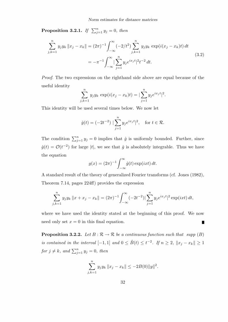
Proposition 3.2.2. Let B : R → R be a continuous function such that supp (B)
is contained in the interval [−1, 1] and 0 ≤ B(t) ≤ t−2. If n ≥ 2, ‖xj − xk‖ ≥ 1
for j 6= k, and∑n
j=1 yj = 0, then
n∑
j,k=1
yjyk ‖xj − xk‖ ≤ −2B(0)‖y‖2.
32

Norm estimates for distance matrices
Proof. By Proposition 3.2.1 and properties of Fourier transforms,
n∑
j,k=1
yjyk ‖xj − xk‖ ≤ (2π)−1
∫ ∞
−∞
(−2B(t))
n∑
j,k=1
yjyk exp(i(xj − xk)t)dt
= −2n∑
j,k=1
yjyk B(xj − xk)
= −2B(0)‖y‖2,
where the first inequality follows from the condition B(t) ≤ t−2. The last line is a
consequence of supp(B) ⊂ [−1, 1].
Corollary 3.2.3. Let
B(x) =
(1 − |x|)/4, if |x| ≤ 10, otherwise.
Then B satisfies the conditions of Proposition 3.2.2 and B(0) = 1/4.
Proof. By direct calculation, we find that
B(t) =sin2(t/2)
t2≤ 1
t2.
It is clear that the other conditions of Proposition 3.2.2 are satisfied.
We have therefore shown the following theorem to be true.
Theorem 3.2.4. Let (xj)n1 be points in R such that n ≥ 2 and ‖xj − xk‖ ≥ 1
when j 6= k. If∑n
j=1 yj = 0, then
n∑
j,k=1
yjyk ‖xj − xk‖ ≤ −1
2‖y‖2.
We see that a consequence of this result is the non-singularity of the Euclidean
distance matrix when the points (xj)n1 are distinct and n ≥ 2. It is important
to realise that the homogeneity of the Euclidean norm allows us to replace the
condition “‖xj − xk‖ ≥ 1 if j 6= k” by “‖xj − xk‖ ≥ ε if j 6= k”. We restate
Theorem 3.2.4 in this form for the convenience of the reader:
33

Norm estimates for distance matrices
Theorem 3.2.4b. Choose any ε > 0 and let (xj)n1 be points in R such that n ≥ 2
and ‖xj − xk‖ ≥ ε when j 6= k. If∑n
j=1 yj = 0, then
n∑
j,k=1
yjyk ‖xj − xk‖ ≤ −1
2ε‖y‖2.
We shall now show that this bound is optimal. Without loss of generality, we
return to the case ε = 1. We take our points to be the integers 0, 1, . . . , n, so that
the Euclidean distance matrix, An say, is given by
An =
0 1 2 . . . n1 0 1 . . . n − 1...
.... . .
...n n − 1 n − 2 . . . 0
.
It is straightforward to calculate the inverse of An:
A−1n =
(1 − n)/2n 1/2 1/2n1/2 −1 1/2
1/2 −1. . .
−1 1/21/2n 1/2 (1 − n)/2n
.
Proposition 3.2.5. We have the inequality 2 − (π2/2n2) ≤ ‖A−1n ‖2 ≤ 2.
Proof. We observe that ‖A−1n ‖2 ≤ ‖A−1
n ‖1 = 2, establishing the upper bound. For
the lower bound, we focus attention on the (n−1)× (n−1) symmetric tridiagonal
minor of A−1n formed by deleting its first and last rows and columns, which we
shall denote by Tn. Thus we have
Tn =
−1 1/21/2 −1 1/2
1/2 −1. . .
−1 1/21/2 −1
.
Now‖Tn‖2 = maxyT A−1
n y : yT y = 1 and y1 = yn+1 = 0
≤ maxyT A−1n y : yT y = 1
= ‖A−1n ‖2,
34

Norm estimates for distance matrices
so that ‖Tn‖2 ≤ ‖A−1n ‖2 ≤ 2. But the eigenvalues of Tn are given by
λk = −1 + cos(kπ/n), for k = 1, 2, . . . , n − 1.
Thus ‖Tn‖2 = 1− cos(π − π/n) ≥ 2− π2/2n2, where we have used an elementary
inequality based on the Taylor series for the cosine function. The proposition is
proved.
3.3. The Multivariate Case for the Euclidean Norm
We first prove the multivariate versions of Propositions 3.2.1 and 3.2.2, which gen-
eralize in a very straightforward way. We shall require the fact that the generalized
Fourier transform of ϕ(x) = ‖x‖ in Rd is given by
ϕ(t) = −cd‖t‖−d−1,
where
cd = 2dπ(d−1)/2Γ((d + 1)/2).
This may be found in Jones (1982), Theorem 7.32. We now deal with the analogue
of Proposition 3.2.1.
Proposition 3.3.1. If∑n
j=1 yj = 0, then
n∑
j,k=1
yjyk ‖xj − xk‖ = −cd(2π)−d
∫
Rd
|n∑
j=1
yjeixjt|2‖t‖−d−1 dt. (3.3)
Proof. We define
g(t) = −cd‖t‖−d−1|n∑
j=1
yjeixjt|2.
The condition∑n
j=1 yj = 0 implies this function is uniformly bounded and the de-
cay for large argument is sufficient to ensure absolute integrability. The argument
now follows the proof of Proposition 3.2.1, with obvious minor changes.
35
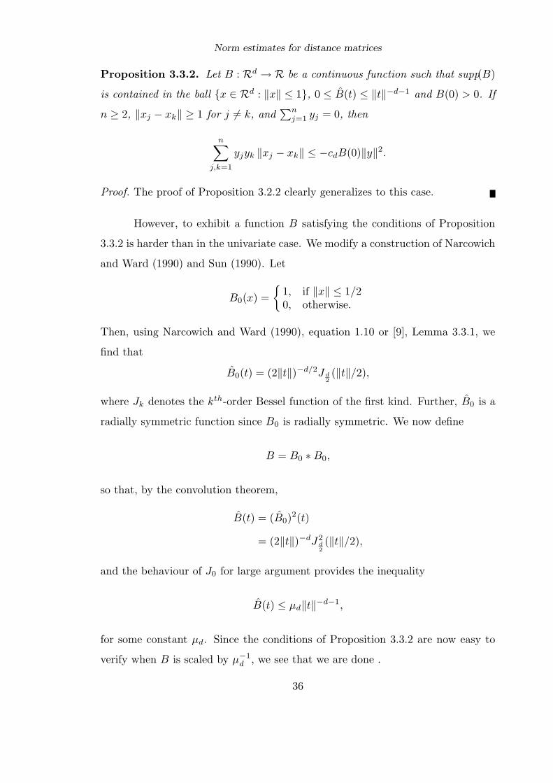
Norm estimates for distance matrices
Proposition 3.3.2. Let B : Rd → R be a continuous function such that supp(B)
is contained in the ball x ∈ Rd : ‖x‖ ≤ 1, 0 ≤ B(t) ≤ ‖t‖−d−1 and B(0) > 0. If
n ≥ 2, ‖xj − xk‖ ≥ 1 for j 6= k, and∑n
j=1 yj = 0, then
n∑
j,k=1
yjyk ‖xj − xk‖ ≤ −cdB(0)‖y‖2.
Proof. The proof of Proposition 3.2.2 clearly generalizes to this case.
However, to exhibit a function B satisfying the conditions of Proposition
3.3.2 is harder than in the univariate case. We modify a construction of Narcowich
and Ward (1990) and Sun (1990). Let
B0(x) =
1, if ‖x‖ ≤ 1/20, otherwise.
Then, using Narcowich and Ward (1990), equation 1.10 or [9], Lemma 3.3.1, we
find that
B0(t) = (2‖t‖)−d/2J d2
(‖t‖/2),
where Jk denotes the kth-order Bessel function of the first kind. Further, B0 is a
radially symmetric function since B0 is radially symmetric. We now define
B = B0 ∗ B0,
so that, by the convolution theorem,
B(t) = (B0)2(t)
= (2‖t‖)−dJ2d2
(‖t‖/2),
and the behaviour of J0 for large argument provides the inequality
B(t) ≤ µd‖t‖−d−1,
for some constant µd. Since the conditions of Proposition 3.3.2 are now easy to
verify when B is scaled by µ−1d , we see that we are done .
36

Norm estimates for distance matrices
3.4. Fourier Transforms and Bessel Transforms
Here we relate our technique to the work of Ball (1989) and Narcowich and Ward
(1990, 1991).
Definition 3.4.1. A real sequence (yj)j∈Zd is said to be zero-summing if it is
finitely supported and∑
j∈Zd yj = 0.
Definition 3.4.2. A function ϕ: [0,∞) → R will be said to be conditionally neg-
ative definite of order 1 on Rd, hereafter shortened to CND1(d), if it is continuous
and, for any points (xj)j∈Zd in Rd and any zero-summing sequence (yj)j∈Zd , we
have∑
j,k∈Zd
yjykϕ(‖xj − xk‖) ≤ 0.
Such functions were characterized by von Neumann and Schoenberg (1941). For
every positive integer d, let Ωd: [0,∞) → R be defined by
Ωd(r) = ωd−1−1
∫
Sd−1
cos(ryu) dy,
where u may be any unit vector in Rd, Sd−1 denotes the unit sphere in Rd, and
ωd−1 its (d−1)-dimensional Lebesgue measure. Thus Ωd is essentially the Fourier
transform of the normalized rotation invariant measure on the unit sphere.
Theorem 3.4.3. Let ϕ: [0,∞) → R be a continuous function. A necessary and
sufficient condition that ϕ be a CND1(d) function is that it have the form
ϕ(r) = ϕ(0) +
∫ ∞
0
(1 − Ωd(rt)) t−2dβ(t),
for every r ≥ 0, where β: [0,∞) → R is a non-decreasing function such that∫ ∞
1t−2 dβ(t) < ∞ and β(0) = 0. Furthermore, β is uniquely determined by ϕ.
Proof. The first part of this result is Theorem 7 of von Neumann and Schoenberg
(1941), restated in our terminology. The uniqueness of β is a consequence of
Lemma 2 of that paper.
37

Norm estimates for distance matrices
It is a consequence of this theorem that there exist constants A and B such that
ϕ(r) ≤ Ar2 + B. For we have
∣∣∣∣∫ ∞
1
(1 − Ωd(rt)) t−2 dβ(t)
∣∣∣∣ ≤ 2
∫ ∞
1
t−2 dβ(t) < ∞,
using the fact that |Ωd(r)| ≤ 1 for every r ≥ 0. Further, we see that
0 ≤ 1 − Ωd(ρ) = 2ωd−1−1
∫
Sd−1
sin2(ρut/2) dt ≤ ρ2/2,
which provides the bound
∣∣∣∫ 1
0
(1 − Ωd(rt)) t−2 dβ(t)∣∣∣ ≤ r2
∫ 1
0
1
2dβ(t) =
1
2r2β(1).
Thus A = β(1)/2 and B = ϕ(0) + 2∫ ∞
1t−2 dβ(t) suffice. Therefore the function
ϕ(‖x‖) : x ∈ Rd is a tempered distribution in the sense of Schwartz (1966) and
possesses a generalized Fourier transform ϕ(‖ξ‖) : ξ ∈ Rd. There is a rather
simple relation between the generalized Fourier transform and the nondecreasing
function of Theorem 3.4.3 for a certain class of functions. This is our next topic.
Definition 3.4.4. A function ϕ: [0,∞) → R will be termed admissible if it is a
continuous function of algebraic growth which satisfies the following conditions:
1. ϕ is a continuous function on Rd \ 0.2. The limit lim ‖ξ‖→0 ‖ξ‖d+1ϕ(‖ξ‖) exists.
3. The integral∫‖ξ‖≥1 |ϕ(‖ξ‖)| dξ exists.
It is straightforward to prove the analogue of Propositions 3.2.1 and 3.3.1
for an admissible function.
Proposition 3.4.5. Let ϕ: [0,∞) → R be an admissible function and let (yj)j∈Zd
be a zero-summing sequence. Then for any choice of points (xj)j∈Zd in Rd we have
the identity
∑
j,k∈Zd
yjykϕ(‖xj − xk‖) = (2π)−d
∫
Rd
∣∣∣∑
j∈Zd
yj exp(ixjξ)∣∣∣2
ϕ(‖ξ‖) dξ. (3.4)
38

Norm estimates for distance matrices
Proof. Let g:Rd → R be the function defined by
g(ξ) =∣∣∣∑
j∈Zd
yj exp(ixjξ)∣∣∣2
ϕ(‖ξ‖).
Then g is an absolutely integrable function on Rd, because of the conditions on
ϕ and because (yj)j∈Zd is a zero-summing sequence. Thus g is the generalized
transform of∑
j,k yjykϕ(‖ ·+xj − xk‖), and by standard properties of generalized
Fourier transforms we deduce that
∑
j,k
yjykϕ(‖x + xj − xk‖) = (2π)−d
∫
Rd
∣∣∣∑
j∈Zd
yj exp(ixjξ)∣∣∣2
ϕ(‖ξ‖) exp(ixξ) dξ.
The proof is completed by setting x = 0.
Proposition 3.4.6. Let ϕ: [0,∞) → R be an admissible CND1(d) function. Then
dβ(t) = −(2π)−dωd−1ϕ(‖tu‖)td+1 dt,
where u may be any unit vector in Rd.
Proof. Let µ and ν be different integers and let (yj)j∈Zd be a sequence with only
two nonzero elements, namely yµ = −yν = 2−1/2. Choose any point ζ ∈ Rd and
set xµ = 0, xν = ζ, so that equation (3.4) provides the expression
ϕ(0) − ϕ(‖ζ‖) = (2π)−d
∫
Rd
(1 − cos(ζξ)) ϕ(‖ξ‖) dξ.
Employing spherical polar coordinates, this integral takes the form
ϕ(0) − ϕ(‖ζ‖) = 2π)−dωd−1
∫ ∞
0
(1 − Ωd(t‖ζ‖)) ϕ(‖tu‖)td−1 dt,
where u may be any unit vector in Rd. Setting r = ‖ζ‖, we have
ϕ(r) = ϕ(0) +
∫ ∞
0
(1 − Ωd(rt)) γ(t)t−2 dt,
where γ(t) = −(2π)−dωd−1ϕ(‖tu‖)td+1. Now Theorem 4.2.6 of the following chap-
ter implies that ϕ is a nonpositive function. Thus there exists a nondecreasing
39
Norm estimates for distance matrices
function β: [0,∞) → R such that γ(t) dt = dβ(t), and∫ ∞
1t−2 dβ(t) is finite and
β(0) = 0. But the uniqueness of the representation of Theorem 3.4.3 implies that
β = β, that is
dβ(t) = −(2π)−dωd−1ϕ(‖tu‖)td+1 dt,
and the proof is complete.
This proposition is useful if we want to calculate β for a particular function
ϕ, since tables of generalized Fourier transforms are readily available.
Example 3.4.7. Let ϕ(r) = (r2+1)1/2. This is a non-negative CND1(d) function
for all d (see Micchelli (1986)). When d = 3, the generalized Fourier transform is
ϕ(r) = −4πr−2K2(r). Here K2 is a modified Bessel function which is positive and
smooth in R+, has a pole at the origin, and decays exponentially (See Abramowitz
and Stegun (1970)). Consequently ϕ is a non-negative admissible function. Ap-
plying Theorem 3.4.7 gives the equation
dβ(r) = (2π)−3(4π)r4(4πr−2K2(r))
= (2r2/π)K2(r)dr,
agreeing with Narcowich and Ward (1991), equation 3.12.
3.5. The Least Upper Bound for Subsets of the Integer Grid
In the next chapter we use extensions of the technique provided here to derive the
the following result.
Theorem 3.5.1. Let ϕ: [0,∞) → R be an admissible function that is not identi-
cally zero, let ϕ(0) ≥ 0, and let ϕ be CND1(d) for every positive integer d. Further,
let (xj)j∈Zd be any elements of Zd and let A = (ϕ(‖xj −xk‖))j,k∈N , where N can
be any finite subset of Zd. Then we have the inequality
‖A−1‖ ≤( ∑
k∈Zd
|ϕ(‖πe + 2πk‖)|)−1
,
where e = [1, . . . , 1]T ∈ Rd and ϕ is the generalized Fourier transform of ϕ.
Moreover, this is the least upper bound valid for all finite subsets of Zd.
40

Norm estimates for distance matrices
Proof. See Section 4.4 of the thesis.
41

4 : Norm estimates for Toeplitz distance matrices I
4.1. Introduction
The multivariate interpolation problem is as follows: given points (xj)nj=1 in Rd
and real numbers (fj)nj=1, construct a function s:Rd → R such that s(xk) = fk,
for k = 1, . . . , n. The radial basis function approach is to choose a univariate
function ϕ: [0,∞) → R, a norm ‖ . ‖ on Rd, and to let s take the form
s(x) =n∑
j=1
yjϕ(‖x − xj‖).
The norm ‖ . ‖ will be the Euclidean norm throughout this chapter. Thus the
radial basis function interpolation problem has a unique solution for any given
scalars (fj)nj=1 if and only if the matrix (ϕ(‖xj − xk‖))n
j,k=1 is invertible. Such
a matrix will, as before, be called a distance matrix. These functions provide a
useful and flexible form for multivariate approximation, but their approximation
power as a space of functions is not addressed here.
A powerful and elegant theory was developed by I. J. Schoenberg and oth-
ers some fifty years ago which may be used to analyse the singularity of distance
matrices. Indeed, in Schoenberg (1938) it was shown that the Euclidean dis-
tance matrix, which is the case ϕ(r) = r, is invertible if n ≥ 2 and the points
(xj)nj=1 are distinct. Further, extensions of this work by Micchelli (1986) proved
that the distance matrix is invertible for several classes of functions, including the
Hardy multiquadric, the only restrictions on the points (xj)nj=1 being that they
are distinct and that n ≥ 2. Thus the singularity of the distance matrix has been
successfully investigated for many useful radial basis functions. In this chapter, we
bound the eigenvalue of smallest modulus for certain distance matrices. Specif-
ically, we provide the greatest lower bound on the moduli of the eigenvalues in
the case when the points (xj)nj=1 form a subset of the integers Zd, our method
of analysis applying to a wide class of functions which includes the multiquadric.
More precisely, let N be any finite subset of the integers Zd and let λNmin be the
42

Norm estimates for Toeplitz distance matrices I
smallest eigenvalue in modulus of the distance matrix (ϕ(‖j − k‖))j,k∈N . Then
the results of Sections 3 and 4 provide the inequality
|λNmin| ≥ Cϕ, (4.1.1)
where Cϕ is a positive constant for which an elegant formula is derived. We also
provide a constructive proof that Cϕ cannot be replaced by any larger number,
and it is for this reason that we shall describe inequality (4.1.1) as an optimal
lower bound. Similarly, we shall say that an upper bound is optimal if none of the
constants appearing in the inequality can be replaced by smaller numbers.
It is crucial to our analysis that the distance matrix (ϕ(‖j −k‖))j,k∈N may
be embedded in the bi-infinite matrix (ϕ(‖j−k‖))j,k∈Zd . Such a bi-infinite matrix
is called a Toeplitz matrix if d = 1. We shall use this name for all values of d,
since we use the multivariate form of the Fourier analysis of Toeplitz forms (see
Grenander and Szego (1984)).
Of course, inequality (4.1.1) also provides an upper bound on the norm
of the inverse of the distance matrices generated by finite subsets of the integers
Zd. This is not the first paper to address the problem of bounding the norms
of inverses of distance matrices and we acknowledge the papers of Ball (1989)
and Narcowich and Ward [1990, 1991], which first interested the author in such
estimates. Their results are not limited to the case when the data points are a
subset of the integers. Instead, they apply when the points satisfy the condition
‖xj − xk‖ ≥ ε for j 6= k, where ε is a positive constant, and they provide lower
bounds on the smallest modulus of an eigenvalue for several functions ϕ, including
the multiquadric. We will find that these bounds are not optimal, except in the
special case of the Euclidean norm in the univariate case. Further, our bounds
apply to all the conditionally negative definite functions of order 1. The definition
of this class of functions may be found in Section 4.3.
As in the previous section, we make extensive use of the theory of gen-
eralized Fourier transforms, for which our principal reference will still be Jones
(1982). These transforms are precisely the Fourier transforms of tempered distri-
43
Norm estimates for Toeplitz distance matrices I
butions constructed in Schwartz (1966). First, however, Section 2 presents several
theorems which require only the classical theory of the Fourier transform. These
results will be necessary in Section 4.3.
4.2. Toeplitz forms and Theta functions
We require several properties of the Fejer kernel, which is defined as follows. For
each positive integer n, the nth univariate Fejer kernel is the positive trigonometric
polynomial
Kn(t) =
n∑
k=−n
(1 − |k|/n) exp(ikt)
=sin2 nt/2
n sin2 t/2.
(4.2.1)
Further, the nth multivariate Fejer kernel is defined by the product
Kn(t1, . . . , td) = Kn(t1)Kn(t2) · · ·Kn(td), t ∈ Rd. (4.2.2)
Lemma 4.2.1. The univariate kernel enjoys the following property: for any con-
tinuous 2π-periodic function f :R → R and for all x ∈ R we have
limn→∞
(2π)−1
∫ 2π
0
Kn(t − x)f(t) dt = f(x).
Moreover, we have the equations
(2π)−1
∫ 2π
0
Kn(t) dt = 1 (4.2.3)
and
Kn(t) =∣∣∣n−1/2
n−1∑
k=0
exp(ikt)∣∣∣2
. (4.2.4)
Proof. Most text-books on harmonic analysis contain the first property and (4.2.3).
For example, see pages 89ff, volume I, Zygmund (1979). It is elementary to deduce
(4.2.4) from (4.2.1).
Lemma 4.2.2. For every continuous [0, 2π]d-periodic function f :Rd → R, the
multivariate Fejer kernel gives the convergence property
limn→∞
(2π)−d
∫
[0,2π]dKn(t − x)f(t) dt = f(x)
44

Norm estimates for Toeplitz distance matrices I
for every x ∈ Rd. Further, Kn is the square of the modulus of a trigonometric
polynomial with real coefficients and
(2π)−d
∫
[0,2π]dKn(t) dt = 1.
Proof. The first property is Theorem 1.20 of chapter 17 of Zygmund (1979). The
last part of the lemma is an immediate consequence of (4.2.3), (4.2.4) and the
definition of the multivariate Fejer kernel.
All sequences will be real sequences here. Further, we shall say that a
sequence (aj)Zd := ajj∈Zd is finitely supported if it contains only finitely many
nonzero terms. The scalar product of two vectors x and y in Rd will be denoted
by xy.
Proposition 4.2.3. Let f :Rd → R be an absolutely integrable continuous func-
tion whose Fourier transform f is also absolutely integrable. Then for any finitely
supported sequence (aj)Zd , and for any choice of points (xj)Zd in Rd, we have the
identity
∑
j,k∈Zd
ajakf(xj − xk) = (2π)−d
∫
Rd
∣∣∣∑
j∈Zd
aj exp(ixjξ)∣∣∣2
f(ξ) dξ.
Proof. The function ∑j,k ajakf(x + xj − xk) : x ∈ Rd is absolutely integrable.
Its Fourier transform is given by
[ ∑
j,k∈Zd
ajakf(· + xj − xk)]∧
(ξ) =∑
j,k∈Zd
ajak exp(i(xj − xk)ξ)f(ξ)
=∣∣∣∑
j∈Zd
aj exp(ixjξ)∣∣∣2
f(ξ), ξ ∈ Rd,
and is therefore absolutely integrable. Therefore the Fourier inversion theorem
states that
∑
j,k∈Zd
ajakf(x + xj − xk) = (2π)−d
∫
Rd
∣∣∣∑
j∈Zd
aj exp(ixjξ)∣∣∣2
f(ξ) exp(ixξ) dξ.
Setting x = 0 produces the stated equation.
45

Norm estimates for Toeplitz distance matrices I
In this dissertation a key role will be played by the symbol function
σ(ξ) =∑
k∈Zd
f(ξ + 2πk), ξ ∈ Rd. (4.2.5)
If f ∈ L1(Rd), then σ is an absolutely integrable function on [0, 2π]d and its
defining series is absolutely convergent almost everywhere. These facts are conse-
quences of the relations
∞ >
∫
Rd
|f(ξ)| dξ =∑
k∈Zd
∫
[0,2π]d|f(ξ + 2πk)| dξ =
∫
[0,2π]d
∑
k∈Zd
|f(ξ + 2πk)| dξ,
the exchange of integration and summation being a consequence of Fubini’s theo-
rem. If the points (xj)Zd are integers, then we readily deduce the following bounds
on the quadratic form.
Proposition 4.2.4. Let f satisfy the conditions of Proposition 4.2.3 and let
(aj)Zd be a finitely supported sequence. Then we have the identity
∑
j,k∈Zd
ajakf(j − k) = (2π)−d
∫
[0,2π]d
∣∣∣∑
j∈Zd
aj exp(ijξ)∣∣∣2
σ(ξ) dξ. (4.2.6)
Further, letting m = infσ(ξ) : ξ ∈ [0, 2π]d and M = supσ(ξ) : ξ ∈ [0, 2π]d, we
have the bounds
m∑
j∈Zd
a2j ≤
∑
j,k∈Zd
ajakf(j − k) ≤ M∑
j∈Zd
a2j .
Proof. Proposition 4.2.3 implies the equation
∑
j,k∈Zd
ajakf(j − k) =∑
k∈Zd
(2π)−d
∫
[0,2π]d
∣∣∣∑
j∈Zd
aj exp(ijξ)∣∣∣2
f(ξ + 2πk) dξ
= (2π)−d
∫
[0,2π]d
∣∣∣∑
j∈Zd
aj exp(ijξ)∣∣∣2
σ(ξ) dξ,
the exchange of integration and summation being justified by Fubini’s theorem.
For the upper bound, the Parseval theorem yields the expressions
∑
j,k∈Zd
ajakf(j − k) = (2π)−d
∫
[0,2π]d
∣∣∣∑
j∈Zd
aj exp(ijξ)∣∣∣2
σ(ξ) dξ
≤ M∑
j∈Zd
a2j .
46

Norm estimates for Toeplitz distance matrices I
The lower bound follows similarly and the proof is complete.
The inequalities of the last proposition enjoy the following optimality prop-
erty.
Proposition 4.2.5. Let f satisfy the conditions of Proposition 4.2.3 and suppose
that the symbol function is continuous. Then the inequalities of Proposition 4.2.4
are optimal lower and upper bounds.
Proof. Let ξM ∈ [0, 2π]d be a point such that σ(ξM ) = M , which exists by con-
tinuity of the symbol function. We shall construct finitely supported sequences
(a(n)j )j∈Zd : n = 1, 2, . . . such that
∑j∈Zd(a
(n)j )2 = 1, for all n, and
limn→∞
∑
j,k∈Zd
a(n)j a
(n)k f(j − k) = M. (4.2.7)
We recall from Lemma 4.2.2 that the multivariate Fejer kernel is the square
of the modulus of a trigonometric polynomial with real coefficients. Therefore
there exists a finitely supported sequence (a(n)j )Zd satisfying the relation
∣∣∣∑
j∈Zd
a(n)j exp(ijξ)
∣∣∣2
= Kn(ξ − ξM ), ξ ∈ Rd. (4.2.8)
Further, the Parseval theorem and Lemma 4.2.2 provide the equations
∑
j∈Zd
(a(n)j )2 = (2π)−d
∫
[0,2π]dKn(ξ − ξM ) dξ = 1
and
limn→∞
(2π)−d
∫
[0,2π]dKn(ξ − ξM )σ(ξ) dξ = σ(ξM ) = M.
It follows from (4.2.6) and (4.2.8) that the limit (4.2.7) holds. The lower bound
of Proposition 4.2.4 is dealt with in the same fashion.
The set of functions satisfying the conditions of Proposition 4.2.5 is non-
void. For example, suppose that we have f(ξ) = O(‖ξ‖−d−δ), for large ‖ξ‖, where
δ is a positive constant. Then the series defining the symbol function σ converges
47

Norm estimates for Toeplitz distance matrices I
uniformly, by the Weierstrass M-test, and σ is continuous, being a uniformly con-
vergent sum of continuous functions. These remarks apply when f is a Gaussian,
which is the subject of the rest of this section. We shall see that the analysis of
the Gaussian provides the key to many of our results.
Proposition 4.2.6. Let λ be a positive constant and let f(x) = exp(−λ‖x‖2), for
x ∈ Rd. Then f satisfies the conditions of Proposition 4.2.5.
Proof. The Fourier transform of f is the function f(ξ) = (π/λ)d/2 exp(−‖ξ‖2/4λ),
which is a standard calculation of the classical theory of the Fourier transform. It
is clear that f satisfies the conditions of Proposition 4.2.3, and that the symbol
function is the expression
σ(ξ) = (π/λ)d/2∑
k∈Zd
exp(−‖ξ + 2πk‖2/4λ), ξ ∈ Rd. (4.2.9)
Finally, the decay of the Gaussian ensures that σ is continuous, being a uniformly
convergent sum of continuous functions.
This result is of little use unless we know the minimum and maximum
values of the symbol function for the Gaussian. Therefore we show next that
explicit expressions for these numbers may be calculated from properties of Theta
functions. Lemmata 4.2.7 and 4.2.8 address the cases when d = 1 and d ≥ 1
respectively.
Lemma 4.2.7. Let λ be a positive constant and let E1:R → R be the 2π-periodic
function
E1(t) =∞∑
k=−∞
exp(−λ(t + 2kπ)2
).
Then E1(0) ≥ E1(t) ≥ E1(π) for all t ∈ R.
Proof. An application of the Poisson summation formula provides the relation
E1(t) = (4πλ)−1/2∞∑
k=−∞
e−k2/4λeikt
= (4πλ)−1/2
(1 + 2
∞∑
k=1
e−k2/4λ cos(kt)
).
48

Norm estimates for Toeplitz distance matrices I
This is a Theta function. Indeed, using the notation of Whittaker and Watson
(1927), Section 21.11, it is a Theta function of Jacobi type
ϑ3(z, q) = 1 + 2
∞∑
k=1
qk2
cos(2kz),
where q ∈ C and |q| < 1. Choosing q = e−1/4λ we obtain the relation
E1(t) = (4πλ)−1/2ϑ3(t/2, q).
The useful product formula for ϑ3:
ϑ3(z, q) = G∞∏
k=1
(1 + 2q2k−1 cos 2z + q4k−2),
where G =∏∞
k=1(1−q2k), is given in Whittaker and Watson (1927), Sections 21.3
and 21.42. Thus
E1(t) = (4πλ)−1/2G∞∏
k=1
(1 + 2q2k−1 cos t + q4k−2), t ∈ R.
Now each term of the infinite product is a decreasing function on the interval
[0, π], which implies that E1 is a decreasing function on [0, π]. Since E1 is an even
2π-periodic function, we deduce that E1 attains its global minimum at t = π and
its maximum at t = 0.
Lemma 4.2.8. Let λ be a positive constant and let Ed:Rd → Rd be the [0, 2π]d-
periodic function given by
Ed(x) =∑
k∈Zd
exp(−λ‖x + 2kπ‖2).
Then Ed(0) ≥ Ed(x) ≥ Ed(πe), where e = [1, 1, . . . , 1]T .
Proof. The key observation is the equation
Ed(x) =
d∏
k=1
E1(xk).
49

Norm estimates for Toeplitz distance matrices I
Thus Ed(0) =∏d
k=1 E1(0) ≥ ∏dk=1 E1(xk) = Ed(x) ≥ ∏d
k=1 E1(π) = Ed(πe),
using the previous lemma.
These lemmata imply that in the Gaussian case the maximum and minimum
values of the symbol function occur at ξ = 0 and ξ = πe respectively, where
e = [1, . . . , 1]T . Therefore we deduce from formula (4.2.9) that the constants of
Proposition 4.2.4 are the expressions
m = (π/λ)d/2∑
k∈Zd
exp(−‖πe + 2πk‖2/4λ) and
M = (π/λ)d/2∑
k∈Zd
exp(−‖πk‖2/λ).(4.2.10)
4.3. Conditionally negative definite functions of order 1
In this section we derive the optimal lower bound on the eigenvalue moduli of the
distance matrices generated by the integers for a class of functions including the
Hardy multiquadric.
Definition 4.3.1. A real sequence (yj)Zd is said to be zero-summing if it is finitely
supported and∑
j∈Zd yj = 0.
Let ϕ: [0,∞) → R be a continuous function of algebraic growth. Thus it is
meaningful to speak of the generalized Fourier transform of the radially symmetric
function ϕ(‖x‖) : x ∈ Rd. We denote this transform by ϕ(‖ξ‖) : ξ ∈ Rd,so emphasizing that it is a radially symmetric distribution, but we note that ϕ
depends on d. We shall restrict attention to the collection of functions described
below.
Definition 4.3.2. A function ϕ: [0,∞) → R will be termed admissible if it is a
continuous function of algebraic growth which satisfies the following conditions:
1. ϕ is a continuous function on Rd \ 0.2. The limit lim ‖ξ‖→0 ‖ξ‖d+1ϕ(‖ξ‖) exists.
3. The integral∫‖ξ‖≥1 |ϕ(‖ξ‖)| dξ exists.
50
Norm estimates for Toeplitz distance matrices I
It is straightforward to prove the analogue of Proposition 4.2.3 for an ad-
missible function.
Proposition 4.3.3. Let ϕ: [0,∞) → R be an admissible function and let (yj)Zd
be a zero-summing sequence. Then for any choice of points (xj)Zd in Rd we have
the identity
∑
j,k∈Zd
yjykϕ(‖xj − xk‖) = (2π)−d
∫
Rd
∣∣∣∑
j∈Zd
yj exp(ixjξ)∣∣∣2
ϕ(‖ξ‖) dξ. (4.3.1)
Proof. Let g:Rd → R be the function defined by
g(ξ) =∣∣∣∑
j∈Zd
yj exp(ixjξ)∣∣∣2
ϕ(‖ξ‖).
Then g is an absolutely integrable function on Rd, because of the conditions on ϕ
and because (yj)Zd is a zero-summing sequence. Thus g is the generalized trans-
form of∑
j,k yjykϕ(‖·+xj−xk‖), and by standard properties of generalized Fourier
transforms we deduce that
∑
j,k
yjykϕ(‖x + xj − xk‖) = (2π)−d
∫
Rd
∣∣∣∑
j∈Zd
yj exp(ixjξ)∣∣∣2
ϕ(‖ξ‖) exp(ixξ) dξ.
The proof is completed by setting x = 0.
We come now to the subject that is given in the title of this section.
Definition 4.3.4. Let ϕ: [0,∞) → R be a continuous function. We shall say that
ϕ is conditionally negative definite of order 1 on every Rd, hereafter shortened to
CND1, if we have the inequality
∑
j,k∈Zd
yjykϕ(‖xj − xk‖) ≤ 0,
for every positive integer d, for every zero-summing sequence (yj)Zd and for any
choice of points (xj)Zd in Rd.
Such functions were completely characterized by I. J. Schoenberg (1938).
51
Norm estimates for Toeplitz distance matrices I
Theorem 4.3.5. A continuous function ϕ: [0,∞) → R is CND1 if and only if
there exists a nondecreasing function α: [0,∞) → R such that
ϕ(r) = ϕ(0) +
∫ ∞
0
[1 − exp(−tr2)]t−1dα(t), for r > 0,
and the integral∫ ∞
1t−1 dα(t) exists.
Proof. This is Theorem 6 of Schoenberg (1938).
Thus dα is a positive Borel measure such that
∫ 1
0
dα(t) < ∞ and
∫ ∞
1
t−1 dα(t) < ∞.
Further, it is a consequence of this theorem that there exist constants A and B
such that ϕ(r) ≤ Ar2 + B, where A and B are constants. In order to prove this
assertion we note the elementary inequalities
∫ ∞
1
[1 − exp(−tr2)]t−1 dα(t) ≤∫ ∞
1
t−1 dα(t) < ∞,
and ∫ 1
0
[1 − exp(−tr2)]t−1 dα(t) ≤ r2
∫ 1
0
dα(t).
Thus A = r2(α(1)−α(0)) and B = ϕ(0)+∫ ∞
1t−1 dα(t) suffice. Therefore we may
regard a CND1 function as a tempered distribution and it possesses a generalized
Fourier transform. The following relation between the transform and the integral
representation of Theorem 4.3.5 will be essential to our needs.
Theorem 4.3.6. Let ϕ: [0,∞) → R be an admissible CND1 function. For ξ ∈Rd \ 0, we have the formula
ϕ(‖ξ‖) = −∫ ∞
0
exp(−‖ξ‖2/4t)(π/t)d/2t−1 dα(t). (4.3.2)
Before embarking on the proof of this theorem, we require some ground-
work. We shall say that a function f :Rd \ 0 → R is symmetric if f(−x) = f(x),
for every x ∈ Rd \ 0.
52
Norm estimates for Toeplitz distance matrices I
Lemma 4.3.7. Let α: [0,∞) → R be a nondecreasing function such that the
integral∫ ∞
1t−1 dα(t) exists. Then the function
ψ(ξ) = −∫ ∞
0
exp(−‖ξ‖2/4t)(π/t)d/2t−1 dα(t), ξ ∈ Rd \ 0, (4.3.3)
is a symmetric smooth function, that is every derivative exists.
Proof. For every nonzero ξ, the limit
limt→0
exp(−‖ξ‖2/4t)(π/t)d/2t−1 = 0
implies that the integrand of expression (4.3.3) is a continuous function on [0,∞).
Therefore it follows from the inequality
∫ ∞
1
exp(−‖ξ‖2/4t)(π/t)d/2t−1 dα(t) ≤ πd/2
∫ ∞
1
t−1 dα(t) < ∞
that the integral is well-defined. Further, a similar argument for nonzero ξ shows
that every derivative of the integrand with respect to ξ is also absolutely inte-
grable for t ∈ [0,∞), which implies that every derivative of ψ exists. The proof is
complete, the symmetry of ψ being obvious.
Lemma 4.3.8. Let f :Rd → R be a symmetric absolutely integrable function such
that ∫
Rd
∣∣∣∑
j∈Zd
aj exp(ixjt)∣∣∣2
f(t) dt = 0,
for every finitely supported sequence (aj)Zd and for any choice of points (xj)Zd .
Then f must vanish almost everywhere.
Proof. The given conditions on f imply that the Fourier transform f is a symmetric
function that satisfies the equation
∑
j,k∈Zd
ajakf(xj − xk) = 0,
for every finitely supported sequence (aj)Zd and for all points (xj)Zd in Rd. Let
α and β be different integers and let aα and aβ be the only nonzero elements of
53
Norm estimates for Toeplitz distance matrices I
(aj)Zd . We now choose any point ξ ∈ Rd \ 0 and set xα = 0, xβ = ξ, which
provides the equation
(aα
aβ
)T (f(0) f(ξ)
f(ξ) f(0)
)(aα
aβ
)= 0, for all aα, aβ ∈ R.
Therefore f(0) = f(ξ) = 0, and since ξ was arbitrary, f can only be the zero
function. Consequently f must vanish almost everywhere.
Corollary 4.3.9. Let g:Rd \ 0 → R be a symmetric continuous function such
that ∫
Rd
∣∣∣∑
j∈Zd
yj exp(ixjξ)∣∣∣2
|g(ξ)| dξ < ∞ (4.3.4)
and ∫
Rd
∣∣∣∑
j∈Zd
yj exp(ixjξ)∣∣∣2
g(ξ) dξ = 0, (4.3.5)
for every zero-summing sequence (yj)Zd and for any choice of points (xj)Zd . Then
g(ξ) = 0 for every ξ ∈ Rd \ 0.
Proof. For any integer k ∈ 1, . . . , d and for any positive real number λ, let h be
the symmetric function
h(ξ) = g(ξ) sin2 λξk, ξ ∈ Rd \ 0.
The relation
h(ξ) = g(ξ)∣∣∣12
exp(iλξk) − 1
2exp(−iλξk)
∣∣∣2
and condition (4.3.4) imply that h is absolutely integrable.
Let (aj)Zd be any real finitely supported sequence and let (bj)Zd be any
sequence of points in Rd. We define a real sequence (yj)Zd and points (xj)Zd in
Rd by the equation
∑
j∈Zd
yj exp(ixjξ) = sinλξk
∑
j∈Zd
aj exp(ibjξ).
54
Norm estimates for Toeplitz distance matrices I
Thus (yj)Zd is a sequence of finite support. Further, setting ξ = 0, we deduce that∑
j∈Zd yj = 0, so (yj)Zd is a zero-summing sequence. By condition (4.3.5), we
have
0 =
∫
Rd
∣∣∣∑
j∈Zd
yj exp(ixjξ)∣∣∣2
g(ξ) dξ =
∫
Rd
∣∣∣∑
j∈Zd
aj exp(ibjξ)∣∣∣2
h(ξ) dξ.
Therefore we can apply Lemma 4.3.8 to h, finding that it vanishes almost every-
where. Hence the continuity of g for nonzero argument implies that g(ξ) sin2 λξk =
0 for ξ 6= 0. But for every nonzero ξ there exist k ∈ 1, . . . , d and λ > 0 such that
sinλξk 6= 0. Consequently g vanishes on Rd \ 0.
We now complete the proof of Theorem 4.3.6.
Proof of Theorem 4.3.6. Let (yj)Zd be a zero-summing sequence and let (xj)Zd
be any set of points in Rd. Then Theorem 4.3.5 provides the expression
∑
j,k∈Zd
yjykϕ(‖xj − xk‖) = −∫ ∞
0
( ∑
j,k∈Zd
yjyk exp(−t‖xj − xk‖2))t−1 dα(t),
this integral being well-defined because of the condition∑
j∈Zd yj = 0. Therefore,
using Proposition 4.2.3 with f(·) = exp(−t‖ · ‖2) in order to restate the Gaussian
quadratic form in the integrand, we find the equation
∑
j,k∈Zd
yjykϕ(‖xj − xk‖)
= −∫ ∞
0
[(2π)−d
∫
Rd
∣∣∣∑
j∈Zd
yj exp(ixjξ)∣∣∣2
(π/t)d/2 exp(−‖ξ‖2/4t) dξ]t−1 dα(t)
= (2π)−d
∫
Rd
∣∣∣∑
j∈Zd
yj exp(ixjξ)∣∣∣2
ψ(ξ) dξ,
where we have used Fubini’s theorem to exchange the order of integration and
where ψ is the function defined in (4.3.3). By comparing this equation with the
assertion of Proposition 4.3.3, we see that the difference g(ξ) = ϕ(‖ξ‖) − ψ(ξ)
satisfies the conditions of Corollary 4.3.9. Hence ϕ(‖ξ‖) = ψ(ξ) for all ξ ∈ Rd \ 0.The proof is complete.
55

Norm estimates for Toeplitz distance matrices I
Remark. An immediate consequence of this theorem is that the generalized
Fourier transform of an admissible CND1 function cannot change sign.
The appearance of the Gaussian quadratic form in the proof of Theorem
4.3.6 enables us to use the bounds of Lemma 4.2.8, which gives the following result.
Theorem 4.3.10. Let ϕ: [0,∞) → R be an admissible CND1 function and let
(yj)Zd be a zero-summing sequence. Then we have the inequality
∣∣∣∑
j,k∈Zd
yjykϕ(‖j − k‖)∣∣∣≥ |σ(πe)|
∑
j∈Zd
y2j ,
where e = [1, . . . , 1]T .
Proof. Applying (4.3.1) and dissecting Rd into integer translates of [0, 2π]d, we
obtain the equations∣∣∣
∑
j,k∈Zd
yjykϕ(‖j − k‖)∣∣∣ = (2π)−d
∫
Rd
∣∣∣∑
j∈Zd
yj exp(ijξ)∣∣∣2
|ϕ(‖ξ‖)| dξ
= (2π)−d
∫
[0,2π]d
∣∣∣∑
j∈Zd
yj exp(ijξ)∣∣∣2
|σ(ξ)| dξ,
(4.3.6)
where the interchange of summation and integration is justified by Fubini’s the-
orem, and where we have used the fact that ϕ does not change sign. Here the
symbol function has the usual form (4.2.5). Further, using (4.3.2), we again apply
Fubini’s theorem to deduce the formula
|σ(ξ)| =∑
k∈Zd
|ϕ(‖ξ + 2πk‖)|
=
∫ ∞
0
( ∑
k∈Zd
exp(−‖ξ + 2πk‖2/4t))
(π/t)d/2t−1dα(t).
It follows from Lemma 4.2.8 that we have the bound
|σ(ξ)| ≥∫ ∞
0
( ∑
k∈Zd
exp(−‖πe + 2πk‖2/4t))
(π/t)d/2t−1dα(t)
= |σ(πe)|.(4.3.7)
The required inequality is now a consequence of (4.3.6) and the Parseval relation
(2π)−d
∫
[0,2π]d
∣∣∣∑
j∈Zd
yj exp(ijξ)∣∣∣2
dξ =∑
j∈Zd
y2j .
56
Norm estimates for Toeplitz distance matrices I
When the symbol function is continuous on Rd \ 2πZd, we can show that
the previous inequality is optimal using a modification of the proof of Proposition
4.2.5. Specifically, we construct a set (y(n)j )Zd : n = 1, 2, . . . of zero-summing
sequences such that limn→∞∑
j∈Zd(y(n)j )2 = 1 and
limn→∞
∣∣∣∑
j,k∈Zd
y(n)j y
(n)k ϕ(‖j − k‖)
∣∣∣= |σ(πe)|,
which implies that we cannot replace |σ(πe)| by any larger number in Theorem
4.3.10.
Corollary 4.3.11. Let ϕ: [0,∞) → R satisfy the conditions of Theorem 4.3.10
and let the symbol function be continuous in the set Rd \ 2πZd. Then the bound
of Theorem 4.3.10 is optimal.
Proof. Let m be an integer such that 4m ≥ d + 1 and let Sm be the trigonometric
polynomial
Sm(ξ) = [d−1d∑
j=1
sin2(ξj/2)]2m, ξ ∈ Rd.
Recalling from Lemma 4.2.2 that the multivariate Fejer kernel is the square of the
modulus of a trigonometric polynomial with real coefficients, we choose a finitely
supported sequence (y(n)j )Zd satisfying the equations
∣∣∣∑
j∈Zd
y(n)j exp(ijξ)
∣∣∣2
= Kn(ξ − πe)Sm(ξ), ξ ∈ Rd. (4.3.8)
Further, setting ξ = 0 we see that (y(n)j )Zd is a zero-summing sequence. Applying
(4.3.6), we find the relation
∣∣∣∑
j,k∈Zd
y(n)j y
(n)k ϕ(‖j − k‖)
∣∣∣= (2π)−d
∫
[0,2π]dKn(ξ − πe)Sm(ξ) |σ(ξ)| dξ. (4.3.9)
Moreover, because the second condition of Definition 4.3.2 implies that Sm|σ| is a
continuous function, Lemma 4.2.2 provides the equations
limn→∞
(2π)−d
∫
[0,2π]dKn(ξ − πe)Sm(ξ) |σ(ξ)| dξ = Sm(πe) |σ(πe)| = |σ(πe)|.
57
Norm estimates for Toeplitz distance matrices I
It follows from (4.3.9) that we have the limit
limn→∞
∣∣∣∑
j,k∈Zd
y(n)j y
(n)k ϕ(‖j − k‖)
∣∣∣= |σ(πe)|.
Finally, since Sm is a continuous function, another application of Lemma
4.2.2 yields the equation
limn→∞
(2π)−d
∫
[0,2π]dKn(ξ − πe)Sm(ξ) dξ = Sm(πe) = 1.
By substituting expression (4.3.8) into the left hand side and employing the Par-
seval relation
(2π)−d
∫
[0,2π]d
∣∣∣∑
j∈Zd
y(n)j exp(ijξ)
∣∣∣2
dξ =∑
j∈Zd
(y(n)j )2
we find the relation limn→∞∑
j∈Zd(y(n)j )2 = 1.
4.4. Applications
This section relates the optimal inequality given in Theorem 4.3.10 to the spec-
trum of the distance matrix, using an approach due to Ball (1989). We apply the
following theorem.
Theorem 4.4.1. Let A ∈ Rn×n be a symmetric matrix with eigenvalues λ1 ≥· · · ≥ λn. Let E be any subspace of Rn of dimension m. Then we have the inequality
maxxT Ax : xT x = 1, x ⊥ E ≥ λm+1.
Proof. This is the Courant-Fischer minimax theorem. See Wilkinson (1965), pages
99ff.
For any finite subset N of Zd, let AN be the distance matrix (ϕ(‖j −k‖))j,k∈N . Further, let the eigenvalues of AN be λ1 ≥ · · · ≥ λ|N |, where |N | is the
cardinality of N , and let λNmin be the smallest eigenvalue in modulus.
58

Norm estimates for Toeplitz distance matrices I
Proposition 4.4.2. Let ϕ: [0,∞) → R be a CND1 function that is not identically
zero. Let ϕ(0) ≥ 0 and let µ be a positive constant such that
∑
j,k∈Zd
yjykϕ(‖j − k‖) ≤ −µ∑
j∈Zd
y2j , (4.4.1)
for every zero-summing sequence (yj)Zd . Then for every finite subset N of Zd we
have the bound
|λNmin| ≥ µ.
Proof. Equation (4.4.1) implies that
yTANy ≤ −µ yT y,
for every vector (yj)j∈N such that∑
j∈N yj = 0. Thus Theorem 4.4.1 implies that
the eigenvalues of AN satisfy −µ ≥ λ2 ≥ · · · ≥ λ|N |, where the subspace E of
that theorem is simply the span of the vector [1, 1, . . . , 1]T ∈ RN . In particular,
0 > λ2 ≥ · · · ≥ λ|N |. This observation and the condition ϕ(0) ≥ 0 provide the
expressions
0 ≤ trace AN = λ1 +
|N |∑
j=2
λj = λ1 −|N |∑
j=2
|λj |.
Hence we have the relations λNmin = λ2 ≤ −µ. The proof is complete.
We now turn to the case of the multiquadric ϕc(r) = (r2 + c2)1/2, in or-
der to furnish a practical example of the above theory. This is a non-negative
CND1 function (see Micchelli (1986)) and its generalized Fourier transform is the
expression
ϕc(‖ξ‖) = −π−1(2πc/‖ξ‖)(d+1)/2K(d+1)/2(c‖ξ‖),
for nonzero ξ, which may be found in Jones (1982). Here Kν(r) : r > 0 is a
modified Bessel function which is positive and smooth in R+, has a pole at the
origin, and decays exponentially (Abramowitz and Stegun (1970)). Consequently,
ϕc is a non-negative admissible CND1 function. Further, the exponential decay of
ϕc ensures that the symbol function
σc(ξ) =∑
k∈Zd
ϕc(‖ξ + 2πk‖) (4.4.2)
59

Norm estimates for Toeplitz distance matrices I
is continuous for ξ ∈ Rd \ 2πZd. Therefore, given any finite subset N of Zd,
Theorem 4.3.10 and Proposition 4.2 imply that the distance matrix AN has every
eigenvalue bounded away from zero by at least
µc =∑
k∈Zd
|ϕc(‖πe + 2πk‖)|, (4.4.3)
where e = [1, 1, . . . , 1]T ∈ Rd. Moreover, Corollary 4.3.11 shows that this bound
is optimal.
It follows from (4.4.3) that µc → 0 as c → ∞, because of the exponential
decay of the modified Bessel functions for large argument. For example, in the
univariate case we have the formula
µc = (4c/π)[K1(cπ) + K1(3cπ)/3 + K1(5cπ)/5 + · · ·
],
and Table 4.1 displays some values of µc. Of course, a practical implication of
this result is that we cannot expect accurate direct solution of the interpolation
equations for even quite modest values of c, at least without using some special
technique.c Optimal bound
1.0 4.319455 × 10⁻²
2.0 2.513366 × 10⁻³
3.0 1.306969 × 10⁻⁴
4.0 6.462443 × 10⁻⁶
5.0 3.104941 × 10⁻⁷
10.0 6.542373 × 10⁻¹⁴
15.0 2.089078 × 10⁻²⁰
Table 4.1: The optimal bound on the smallest eigenvalue as c → ∞
The optimal bound is achieved only when the numbers of centres is infi-
nite. Therefore it is interesting to investigate how rapidly |λNmin| converges to the
optimal lower bound as |N | increases. Table 4.2 displays |λNmin| = µc(n), say, for
the distance matrix (ϕc(‖j − k‖))n−1j,k=0 for several values of n when c = 1. The
60
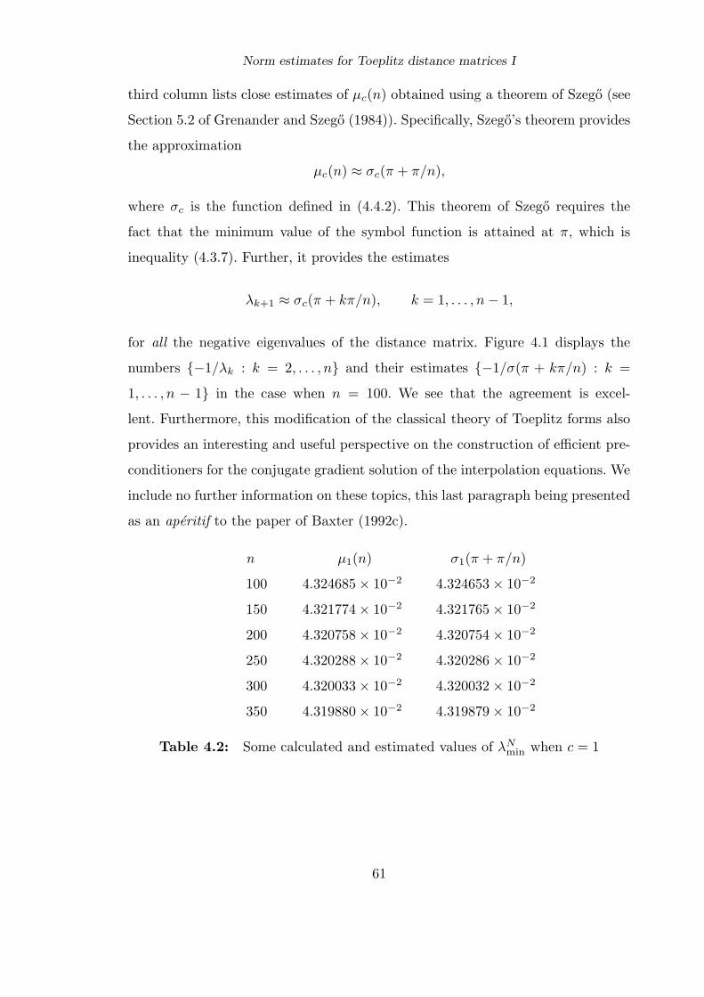
Norm estimates for Toeplitz distance matrices I
third column lists close estimates of µc(n) obtained using a theorem of Szego (see
Section 5.2 of Grenander and Szego (1984)). Specifically, Szego’s theorem provides
the approximation
µc(n) ≈ σc(π + π/n),
where σc is the function defined in (4.4.2). This theorem of Szego requires the
fact that the minimum value of the symbol function is attained at π, which is
inequality (4.3.7). Further, it provides the estimates
λk+1 ≈ σc(π + kπ/n), k = 1, . . . , n − 1,
for all the negative eigenvalues of the distance matrix. Figure 4.1 displays the
numbers −1/λk : k = 2, . . . , n and their estimates −1/σ(π + kπ/n) : k =
1, . . . , n − 1 in the case when n = 100. We see that the agreement is excel-
lent. Furthermore, this modification of the classical theory of Toeplitz forms also
provides an interesting and useful perspective on the construction of efficient pre-
conditioners for the conjugate gradient solution of the interpolation equations. We
include no further information on these topics, this last paragraph being presented
as an aperitif to the paper of Baxter (1992c).
n µ1(n) σ1(π + π/n)
100 4.324685 × 10⁻² 4.324653 × 10⁻²
150 4.321774 × 10⁻² 4.321765 × 10⁻²
200 4.320758 × 10⁻² 4.320754 × 10⁻²
250 4.320288 × 10⁻² 4.320286 × 10⁻²
300 4.320033 × 10⁻² 4.320032 × 10⁻²
350 4.319880 × 10⁻² 4.319879 × 10⁻²
Table 4.2: Some calculated and estimated values of λNmin when c = 1
61

Norm estimates for Toeplitz distance matrices I
0
5
10
15
20
25
0 10 20 30 40 50 60 70 80 90 100
+++++++++++++++++++++++++++++++++++++++++++++++++++++++++++++++++++++++++++++++++++++++++++++++++++
xxxxxxxxxxxxxxxxxxxxxxxxxxxxxxxxxxxxxxxxxxxxxxxxxxxxxxxxxxxxxxxxxxxxxxxxxxxxxxxxxxxxxxxxxxxxxxxxxxx
Key: + - calculated, x - estimated
Figure 4.1. Spectral estimates for a distance matrix of order 100
4.5. A stability estimate
The purpose of this last note is to derive an optimal inequality of the form
∫
Rd
∣∣∣∣∣∣∑
j∈Zd
yjϕ(‖x − j‖)
∣∣∣∣∣∣
2
dx ≥ Cϕ
∑
j∈Zd
y2j ,
where (yj)j∈Zd is a real sequence of finite support such that∑
j∈Zd yj = 0, and
ϕ: [0,∞) → R belongs to a certain class of functions including the multiquadric.
Specifically, this is the class of admissible CND1 functions. These functions have
62

Norm estimates for Toeplitz distance matrices I
generalized Fourier transforms given by
ϕ(‖ξ‖) = −∫ ∞
0
exp(−‖ξ‖2/t) dµ(t), (4.5.1),
where dµ is a positive (but not finite) Borel measure on [0,∞). A derivation of
this expression may be found in Theorem 4.2.6 above.
Lemma 4.5.1. Let (yj)j∈Zd be a zero-summing sequence and let ϕ: [0,∞) → Rbe an admissible CND1 function. Then we have the equation
∫
Rd
∣∣∣∣∣∣∑
j∈Zd
yjϕ(‖x − j‖)
∣∣∣∣∣∣
2
dx = (2π)−d
∫
[0,2π]d|
∑
j∈Zd
yj exp(ijξ)|2σ(ξ) dξ,
where σ(ξ) =∑
k∈Zd |ϕ(‖ξ + 2πk‖)|2.
Proof. Applying the Parseval theorem and dissecting Rd into copies of the cube
[0, 2π]d, we obtain the equations
∫
Rd
|∑
j∈Zd
yjϕ(‖x − j‖)|2 dx
= (2π)−d
∫
Rd
|∑
j∈Zd
yj exp(ijξ)|2|ϕ(‖ξ‖)|2 dξ
=∑
k∈Zd
(2π)−d
∫
[0,2π]d|
∑
j∈Zd
yj exp(ijξ)|2|ϕ(‖ξ + 2πk‖)|2 dξ
= (2π)−d
∫
[0,2π]d|
∑
j∈Zd
yj exp(ijξ)|2σ(ξ) dξ,
where the interchange of summation and integration is justified by Fubini’s theo-
rem.
If σ(ξ) ≥ m for almost every point ξ in [0, 2π]d, then the import of Lemma
4.5.1 is the bound
∫
Rd
∣∣∣∣∣∣∑
j∈Zd
yjϕ(‖x − j‖)
∣∣∣∣∣∣
2
dx ≥ m∑
j∈Zd
y2j .
63
Norm estimates for Toeplitz distance matrices I
We shall prove that we can take m = σ(πe), where e = [1, 1, . . . , 1]T ∈ Rd. Further,
we shall show that the inequality is optimal if the function σ is continuous at the
point πe.
Equation (4.5.1) is the key to this analysis, just as before. We see that
|ϕ(‖ξ‖)|2 =
∫ ∞
0
∫ ∞
0
exp(−‖ξ‖2(t−11 + t−1
2 )) dµ(t1) dµ(t2),
whence,
σ(ξ) =
∫ ∞
0
∫ ∞
0
∑
k∈Zd
exp(−‖ξ + 2πk‖2(t−11 + t−1
2 )) dµ(t1) dµ(t2), (4.5.2),
where the interchange of summation and integration is justified by Fubini’s theo-
rem.
Now it is proved in Lemma 4.1.8 that
∑
k∈Zd
exp(−λ‖ξ + 2πk‖2) ≥∑
k∈Zd
exp(−λ‖πe + 2πk‖2),
for any positive constant λ. Therefore equation (4.5.2) provides the inequality
σ(ξ) ≥∫ ∞
0
∫ ∞
0
∑
k∈Zd
exp(−‖πe + 2πk‖2(t−11 + t−1
2 )) dµ(t1) dµ(t2),
= σ(πe),
which is the promised value of the lower bound m on σ mentioned above. Thus
we have proved the following theorem.
Theorem 4.5.2. Let (yj)j∈Zd , ϕ and σ be as defined in Lemma 1. Then we have
the inequality
∫
Rd
∣∣∣∣∣∣∑
j∈Zd
yjϕ(‖x − j‖)
∣∣∣∣∣∣
2
dx ≥ σ(πe)∑
j∈Zd
y2j .
The proof that this bound is optimal uses the technique of Theorem 4.2.11.
Theorem 4.5.3. The inequality of Theorem 2 is optimal if σ is continuous at πe.
64

Norm estimates for Toeplitz distance matrices I
Proof. The condition that ϕ be admissible requires the existence of the limit
lim‖ξ‖→0 ‖ξ‖d+1ϕ(‖ξ‖).Let m be a positive integer such that 2m ≥ d + 1 and
let us define a sequence (y(n)j )j∈Zd : n = 1, 2, . . . by
∣∣∣∣∣∣∑
j∈Zd
y(n)j exp(ijξ)
∣∣∣∣∣∣
2
=
d−1
d∑
j=1
sin2(ξj/2)
2m
Kn(ξ − πe),
where Kn denotes the multivariate Fejer kernel. The standard properties of the
Fejer kernel needed for this proof are described in Lemma 4.1.2. They allow us to
deduce that (y(n)j )j∈Zd is a zero-summing for every n. Further, we see that
∑
j∈Zd
|y(n)j |2 = (2π)−d
∫
[0,2π]dKn(ξ − πe)(d−1
d∑
j=1
sin2(ξj/2))2m dξ
= 1, for n ≥ 4m.
Finally, m has been chosen so that the function
d−1
d∑
j=1
sin2(ξj/2)
2m
σ(ξ) : ξ ∈ [0, 2π]d
is continuous. Therefore, we have
limn→∞
∫
Rd
∣∣∣∣∣∣∑
j∈Zd
yjϕ(‖x − j‖)
∣∣∣∣∣∣
2
dx
= limn→∞
(2π)−d
∫
[0,2π]dKn(ξ − πe)(d−1
d∑
j=1
sin2(ξj/2))2mσ(ξ) dξ
= σ(πe),
using the fact that σ is continuous at πe and standard properties of the Fejer
kernel.
4.6. Scaling the infinite grid
Here we consider the behaviour of the norm estimate given above when we scale
the infinite regular grid.
65
Norm estimates for Toeplitz distance matrices I
Proposition 4.6.1. Let r be a positive number and let (aj)j∈Zd be a real sequence
of finite support. Then
∑
j,k∈Zd
ajak exp(−‖rj−rk‖2) = (2π)−d
∫
[0,2π]d
∣∣∣∑
j∈Zd
aj exp ijξ∣∣∣2
E(d)r (ξ) dξ, (4.6.1)
where
E(d)r (ξ) =
∑
k∈Zd
e−‖rk‖2
exp ikξ, ξ ∈ Rd. (4.6.2)
Proof. Section 4.2 provides the equation
∑
j,k∈Zd
ajak exp(−‖rj − rk‖2)
= (2π)−d
∫
[0,2π]d
∣∣∣∑
j∈Zd
aj exp ijξ∣∣∣2
(π/r2)d/2∑
k∈Zd
exp(−‖ξ + 2πk‖2/4r2) dξ.
(4.6.3)
Further, the Poisson summation formula gives the relation
(2π)d∑
k∈Zd
exp(−‖ξ + 2πk‖2/4r2) = (4πr2)d/2∑
k∈Zd
e−‖rk‖2
exp ikξ. (4.6.4)
Substituting (4.6.4) into (4.6.3) yields equations (4.6.1) and (4.6.2).
The functions E(1)r and E
(d)r are related in a simple way.
Lemma 4.6.2. We have the expression
E(d)r (ξ) =
d∏
k=1
E(1)r (ξk). (4.6.5)
Proof. This is a straightforward consequence of (4.6.2).
Applying the theta function formulae of Section 4.2 yields the following
result.
Lemma 4.6.3.
E(1)r (ξ) =
∞∏
k=1
(1 − e−2kr2
)(1 + 2e−(2k−1)r2
cos ξ + e−(4k−2)r2
). (4.6.6)
66

Norm estimates for Toeplitz distance matrices I
Proof. The Theta function θ3 of Jacobi type is given by
θ3(z, q) = 1 + 2
∞∑
k=1
qk2
cos 2kz, q, z ∈ C, |q| < 1,
=∞∏
k=1
(1 − q2k)(1 + 2q2k−1 cos 2z + q4k−2),
(4.6.7)
which equations are discussed in greater detail in Section 4.2. Setting q = e−r2
we
have the expressions
E(1)r (ξ) = θ3(ξ/2, q) =
∞∏
k=1
(1− e−2kr2
)(1+2e−(2k−1)r2
cos ξ + e−(4k−2)r2
). (4.6.8)
The proof is complete.
Now Section 4.3 provides the inequality
∑
j,k∈Zd
ajak exp(−‖rj − rk‖2) ≥ E(d)r (πe)
∑
j∈Zd
a2j , (4.6.9)
where e = [1, . . . , 1]T ∈ Rd. Using equation (4.6.6), we see that
E(1)r (π) =
∞∏
k=1
(1 − e−2kr2
)(1 − 2e−(2k−1)r2
+ e−(4k−2)r2
)
=
∞∏
k=1
(1 − e−2kr2
)(1 − e−(2k−1)r2
)2,
(4.6.10)
which implies that E(π)r : r > 0 is an increasing function. Further, it is a conse-
quence of (4.6.5) that E(d)r (πe) : r > 0 is also an increasing function. We state
these results formally.
Theorem 4.6.4. Let r > s > 0. Then we have the inequality
inf∑
j,k∈Zd
ajak exp(−‖rj − rk‖2) ≥ inf∑
j,k∈Zd
ajak exp(−‖sj − sk‖2), (4.6.11)
where the infima are taken over the set of real sequences of finite support.
67

Norm estimates for Toeplitz distance matrices I
In fact we extend the given analysis to a class of functions including the
multiquadric. The appropriate definitions and theorems form Section 4.3, but the
key result is Theorem 4.3.6: Under suitable conditions, the function ϕ: [0,∞) → Rpossesses the generalized Fourier transform
ϕ(‖ξ‖) = −∫ ∞
0
exp(−‖ξ‖2/4t)t−1 dµ(t), (4.6.11)
where
ϕ(r) = ϕ(0) +
∫ ∞
0
(1 − e−r2t)t−1 dµ(t), (4.6.12)
and µ is a positive Borel measure such that∫ 1
0dµ(t) < ∞ and
∫ ∞
1t−1 dµ(t) < ∞.
Now the function ϕr:x 7→ ϕ(‖rx‖) has the Fourier transform
ϕr(‖ξ‖) = ϕ(‖ξ‖/r)r−d. (4.6.13)
Further, the associated symbol function is defined by the equation
σr(ξ) =∑
k∈Zd
|ϕr(‖ξ + 2πk‖)|, (4.6.14)
and so (4.6.13) implies the expression
σr(ξ) =
∫ ∞
0
r−d∑
k∈Zd
exp(−‖ξ + 2πk‖2/4tr2)(π/t)d/2t−1 dµ(t). (4.6.15)
Using the Poisson summation formula, we have
(2π)d∑
k∈Zd
exp(−‖ξ + 2πk‖2/4tr2) = (4tr2π)d/2∑
k∈Zd
e−‖k‖2tr2
eikξ. (4.6.16)
Consequently we have
r−d(π/t)d/2∑
k∈Zd
exp(−‖ξ + 2πk‖2/4tr2) =∑
k∈Zd
e−‖k‖2r2teikξ = E(d)
rt1/2(ξ),
(4.6.18)
providing the equation
σr(πe) =
∫ ∞
0
E(d)
rt1/2(πe)t−1 dµ(t), (4.6.18)
and so σr(πe) : r > 0 is an increasing function.
68

Norm estimates for Toeplitz distance matrices I
Appendix
I do not like stating integral representations such as Theorem 4.3.5 without in-
cluding some explicit examples. Therefore this appendix calculates dα for ϕ(r) = r
and ϕ(r) = (r2 + c2)1/2, where c is positive and we are using the notation of 4.3.5.
For ϕ(r) = r the key integral is
Γ(−1
2) =
∫ ∞
0
(e−u − 1
)u−3/2 du, (A1)
which is derived in Whittaker and Watson (1927), Section 12.21. Making the sub-
stitution u = r2t in (A1) and using the equations π1/2 = Γ(1/2) = −Γ(−1/2)/2
we have
−(4π)1/2 = r−1
∫ ∞
0
(e−r2t − 1
)t−3/2 dt,
that is
r =
∫ ∞
0
(1 − e−r2t
)t−1 (4πt)−1/2 dt. (A2)
Thus the Borel measure is dα1(t) = (4πt)−1/2 dt and∫ 1
0dα1(t) =
∫ ∞
1t−1 dα1(t) =
π1/2.
The representation for the multiquadric is an easy consequence of (A2).
Substituting (r2 + c2)1/2 and c for r in (A2) we obtain
(r2 + c2)1/2 =
∫ ∞
0
(1 − e−(r2+c2)t
)t−1 (4πt)−1/2 dt (A3)
and
c =
∫ ∞
0
(1 − e−c2t
)t−1 (4πt)−1/2 dt, (A4)
respectively. Subtracting (A4) from (A3) provides the formula
(r2 + c2)1/2 = c +
∫ ∞
0
(1 − e−r2t
)t−1 e−c2t(4πt)−1/2 dt. (A5)
Hence the measure is dα2(t) = e−c2t(4πt)−1/2 dt.
69
5 : Norm estimates for Toeplitz distance matrices II
5.1. Introduction
Let ϕ:Rd → R be an even continuous function of at most polynomial growth. As-
sociated with this function is a symmetric bi-infinite multivariate Toeplitz matrix
Φ = (ϕ(j − k))j,k∈Zd . (5.1.1)
Every finite subset I = (ij)nj=1 of Zd determines a finite submatrix of Φ given by
ΦI := (ϕ(ij −k k))nj,k=1 . (5.1.2)
We are interested in upper bounds on the `2-norm of the inverse matrix Φ−1, that
is the quantity
‖Φ−1I ‖ = 1
/min‖x‖2 : ‖ΦIx‖2 = 1, x ∈ RI, (5.1.3)
where ‖x‖22 =
∑j∈I x2
j for x = (xj)j∈I . The type of bound we seek follows the
pattern of results in the previous chapter. Specifically, we let ϕ be the distributional
Fourier transform of ϕ in the sense of Schwartz (1966), which we assume to be a
measurable function on Rd. We let e := (1, . . . , 1)T ∈ Rd and set
τϕ :=∑
j∈Zd
|ϕ(πe + 2πj)| (5.1.4)
whenever the right hand side of this equation is meaningful. Then, for a certain
class of radially symmetric functions, we proved in Chapter 4 that
‖Φ−1I ‖ ≤ 1/τϕ (5.1.5)
for every finite subset I of Zd. Here we extend this bound to a wider class of
functions which need not be radially symmetric. For instance, we show that (5.1.5)
holds for the class of functions
ϕ(x) = (‖x‖1 + c)γ , x ∈ Rd,
70

Norm estimates for Toeplitz distance matrices II
where ‖x‖1 =∑d
j=1 |xj | is the `1-norm of x, c is non-negative, and 0 < γ < 1.
Our analysis develops the methods of Chapter 4. However, here we empha-
size the importance of certain properties of Polya frequency functions and Polya
frequency sequences (due to I. J. Schoenberg) in order to obtain estimates like
(5.1.5).
In Section 2 we consider Fourier transform techniques which we need to
prove our bound. Further, the results of this section improve on the treatment
of the last chapter, in that the condition of admissibility (see Definition 5.3.2) is
shown to be unnecessary. Section 3 contains a discussion of the class of functions
ϕ for which we will prove the bound (5.1.4). The final section contains the proof
of our main result.
5.2. Preliminary facts
We begin with a rather general framework. Let ϕ:Rd → R be a continuous func-
tion of polynomial growth. Thus ϕ possesses a distributional Fourier transform
in the sense of Schwartz (1966). We shall assume ϕ is almost everywhere equal
to a Lebesgue measurable function on Rd, that is we assume ϕ to be the sum
of a measurable function and a tempered distribution whose support is a set of
Lebesgue measure zero. Given a nonzero real sequence (yj)j∈Zd of finite support
and points (xj)j∈Zd in Rd, we introduce the function F :Rd → R given by
F (x) =∑
j,k∈Zd
yjykϕ(x + xj − xk), x ∈ Rd. (5.2.1)
Thus
F (0) =∑
j,k∈Zd
yjykϕ(xj − xk), (5.2.2)
which is the quadratic form whose study is the object of much of this dissertation.
We observe that the Fourier transform of F is the tempered distribution
F (ξ) =∣∣∣∑
j∈Zd
yjeixjξ
∣∣∣2
ϕ(ξ), ξ ∈ Rd. (5.2.3)
71

Norm estimates for Toeplitz distance matrices II
Further, if F is an absolutely integrable function, then we have the equation
F (0) = (2π)−d
∫
Rd
F (ξ) dξ, (5.2.4)
since F is the inverse distributional Fourier transform of F and this coincides with
the classical inverse transform when F ∈ L1(Rd). In other words, we have the
equation
∑
j,k∈Zd
yjykϕ(xj − xk) = (2π)−d
∫
Rd
∣∣∣∑
j∈Zd
yjeixjξ
∣∣∣2
ϕ(ξ) dξ (5.2.5)
when F is absolutely integrable. If we make the further assumption that ϕ is one-
signed almost everywhere on Rd, and the points (xj)j∈Zd form a subset of the
integers Zd, then it is possible to improve (5.2.5). First observe that dissecting Rd
into 2π-integer translates of the cube [0, 2π]d provides the relations
∑
j,k∈Zd
yjykϕ(j − k) = (2π)−d
∫
Rd
∣∣∣∑
j∈Zd
yjeijξ
∣∣∣2
ϕ(ξ) dξ
=∑
k∈Zd
(2π)−d
∫
[0,2π]d
∣∣∣∑
j∈Zd
yjeijξ
∣∣∣2
ϕ(ξ + 2πk) dξ
= (2π)−d
∫
[0,2π]d
∣∣∣∑
j∈Zd
yjeijξ
∣∣∣2
σ(ξ) dξ,
(5.2.6)
where
σ(ξ) =∑
k∈Zd
ϕ(ξ + 2πk), ξ ∈ Rd, (5.2.7)
and the monotone convergence theorem justifies the exchange of summation and
integration. Further, we see that another consequence of the condition that ϕ be
one-signed is the bound ∣∣∣∑
j∈Zd
yjeijξ
∣∣∣2
|ϕ(ξ)| < ∞
for almost every point ξ ∈ [0, 2π]d, because the left hand side of (5.2.6) is a
fortiori finite. This implies that σ is almost everywhere finite, since the set of all
zeros of a nonzero trigonometric polynomial has measure zero. This last result
is well-known, but we include its short proof for completeness. Following Rudin
72

Norm estimates for Toeplitz distance matrices II
(1973), we shall say that a continuous function f : Cd → C is an entire function of d
complex variables if, for every point (w1, . . . , wd) ∈ Cd and for every j ∈ 1, . . . , d,the mapping
C 3 z 7→ f(w1, . . . , wj−1, z, wj+1, . . . , wd)
is an entire function of one complex variable.
Lemma 5.2.1. Given complex numbers (aj)nj=1 and a set of distinct points (xj)n
1
in Rd, we let p:Rd → C be the function
p(ξ) =n∑
j=1
ajeixjξ, ξ ∈ Rd.
Then p enjoys the following properties:
(i) p is identically zero if and only if aj = 0, 1 ≤ j ≤ n.
(ii) p is nonzero almost everywhere unless aj = 0, 1 ≤ j ≤ n.
Proof.
(i) Suppose p is identically zero. Choose any j ∈ 1, . . . , n and let fj :Rd → R be
a continuous function of compact support such that fj(xk) = δjk for 1 ≤ k ≤ n.
Then
aj =n∑
k=1
akfj(xk) = (2π)−d
∫
Rd
n∑
k=1
akeixkξ fj(ξ) dξ = 0.
The converse is obvious.
(ii) Let f : Cd → C be an entire function and let
Z = x ∈ Rd : f(x) = 0.
If voldZ is a set of positive Lebesgue measure in Rd, then we shall prove that f is
identically zero, which implies the required result.
We proceed by induction on the dimension d. If d = 1 and vol1Z > 0,
then f is an entire function of one complex variable with uncountably many zeros.
Such a function must vanish everywhere, because every uncountable subset of Cpossesses a limit point. Now suppose that the result is true for d − 1 for some
d ≥ 2. Fubini’s theorem provides the relation
0 < voldZ =
∫
Rd−1
vol1Z(x2, . . . , xd) dx2 . . . dxd,
73
Norm estimates for Toeplitz distance matrices II
where
Z(x2, . . . , xd) = x1 ∈ R : (x1, . . . , xd) ∈ Z.
Thus there is a set, X say, in Rd−1 of positive (d − 1)-dimensional Lebesgue
measure such that vol1Z(x2, . . . , xd) is positive for every (x2, . . . , xd) ∈ X, and
therefore the entire function C 3 z 7→ f(z, x2, . . . , xd) vanishes for all z ∈ C,
because Z(x2, . . . , xd) is an uncountable set. Thus, choosing any z1 ∈ C, we see
that the entire function of d − 1 complex variables defined by
(z2, . . . , zd) 7→ f(z1, z2, . . . , zd), (z2, . . . , zd) ∈ Cd−1,
vanishes for all (z2, . . . , zd) in X, which is a set of positive (d − 1)- dimensional
Lebesgue measure. By induction hypothesis, we deduce that
f(z1, z2, . . . , zd) = 0 for all z2, . . . , zd ∈ C,
and since z1 can be any complex number, we conclude that f is identically zero.
Therefore the lemma is true.
We can now derive our first bounds on the quadratic form (5.2.2). For
any measurable function g: [0, 2π]d → R, we recall the definitions of the essential
supremum
ess sup g = infc ∈ R : g(x) ≤ c for almost every x ∈ [0, 2π]d (5.2.8)
and the essential infimum
ess inf g = supc ∈ R : g(x) ≥ c for almost every x ∈ [0, 2π]d. (5.2.9)
Thus (5.2.6) and the Parseval relation provide the inequalities
ess inf σ∑
j∈Zd
y2j ≤
∑
j,k∈Zd
yjykϕ(xj − xk) ≤ ess sup σ∑
j∈Zd
y2j . (5.2.10)
Let V be the vector space of real sequences (yj)j∈Zd of finite support for which
the function F of (5.2.3) is absolutely integrable. We have seen that (5.2.10) is
valid for every element (yj)j∈Zd of V . Of course, at this stage there is no guarantee
that V 6= 0 or that the bounds are finite. Nevertheless, we identify below a case
when the bounds (5.2.10) cannot be improved. This will be of relevance later.
74

Norm estimates for Toeplitz distance matrices II
Proposition 5.2.2. Let P be a nonzero trigonometric polynomial such that the
principal ideal I generated by P , that is the set
I = PT : T a real trigonometric polynomial, (5.2.11)
consists of trigonometric polynomials whose Fourier coefficient sequences are ele-
ments of V . Further, suppose that there is a point η at which σ is continuous and
P (η) 6= 0. Then we can find a sequence (y(n)j )j∈Zd : n = 1, 2, . . . in V such that
limn→∞
∑
j,k∈Zd
y(n)j y
(n)k ϕ(j − k)
/ ∑
j∈Zd
[y(n)j ]2 = σ(η). (5.2.12)
Proof. We recal Section 4 and recall that the nth degree tensor product Fejer
kernel is defined by
Kn(ξ) :=d∏
j=1
sin2 nξj/2
n sin2 ξj/2=
∣∣∣n−d/2∑
k∈Zd
0≤k<en
eikξ∣∣∣2
=: |Ln(ξ)|2, ξ ∈ Rd, (5.2.13)
where e = (1, . . . , 1)T ∈ Rd and Ln(ξ) = n−d/2∑
0≤k<en eikξ. Then the function
P (·)Ln(·−η) is a member of I and we choose (y(n)j )j∈Zd to be its Fourier coefficient
sequence. The Parseval relation provides the equation
∑
j∈Zd
[y(n)j ]2 = (2π)−d
∫
[0,2π]dP 2(ξ)Kn(ξ − η) dξ (5.2.14)
and the approximate identity property of the Fejer kernel (Zygmund (1988), p.86)
implies that
P 2(η) = limn→∞
(2π)−d
∫
[0,2π]dP 2(ξ)Kn(ξ − η) dξ
= limn→∞
∑
j∈Zd
[y(n)j ]2.
(5.2.15)
Further, because σ is continuous at η, we also have the relations
P 2(η)σ(η) = limn→∞
(2π)−d
∫
[0,2π]dP 2(ξ)Kn(ξ − η)σ(ξ) dξ
= limn→∞
∑
j,k∈Zd
y(n)j y
(n)k ϕ(j − k),
(5.2.16)
75

Norm estimates for Toeplitz distance matrices II
the last line being a consequence of (5.2.6). Hence (5.2.15) and (5.2.16) provide
equation (5.2.12).
Corollary 5.2.3. If σ attains its essential infimum (resp. supremum) at a point
of continuity, and if we can find a trigonometric polynomial P satisfying the con-
ditions of Proposition 5.2.2, then the lower (resp. upper) bound of (5.2.10) cannot
be improved.
Proof. This is an obvious consequence of Proposition 5.2.2.
We now specialize this general setting to the following case.
Definition 5.2.4. Let G:Rd → R be a continuous absolutely integrable function
such that G(0) = 1 for which the Fourier transform is non-negative and absolutely
integrable. Further, we require that there exist non-negative constants C and κ
for which
|1 − G(x)| ≤ C‖x‖κ, x ∈ Rd. (5.2.17)
We let G denote the class of all such functions G.
Clearly the Gaussian G(x) = exp(−‖x‖2) provides an example of such a
function. The next lemma mentions some salient properties of G which do not,
however, require (5.2.17).
Lemma 5.2.5. Let G ∈ G.
(i) G is a symmetric function, that is
G(x) = G(−x), x ∈ Rd. (5.2.18)
(ii)
|G(x)| ≤ 1, x ∈ Rd. (5.2.19)
(iii) G is a positive definite function in the sense of Bochner. In other words, for
any real sequence (yj)j∈Zd of finite support, and for any points (xj)j∈Zd in
Rd, we have∑
j,k∈Zd
yjykG(xj − xk) ≥ 0. (5.2.20)
76

Norm estimates for Toeplitz distance matrices II
Proof.
(i) Since G is real-valued we have
2i
∫
Rd
G(x) sinxξ dx = G(ξ) − G(−ξ) ∈ R, ξ ∈ Rd,
which is a contradiction unless both sides vanish. Thus G is a symmetric
function. However, G must inherit this symmetry, by the Fourier inversion
theorem.
(ii) The non-negativity of G provides the relations
|G(x)| =∣∣∣(2π)−d
∫
Rd
G(ξ)e−ixξ dξ∣∣∣ ≤ (2π)−d
∫
Rd
G(ξ) dξ = G(0) = 1.
(iii) The condition G ∈ L1(Rd) implies the validity of (5.2.5) for ϕ replaced by
G, whence
∑
j,k∈Zd
yjykG(xj − xk) = (2π)−d
∫
Rd
∣∣∣∑
j∈Zd
yjeixjξ
∣∣∣2
G(ξ) dξ ≥ 0,
as required.
We remark that the first two parts of Lemma 5.2.5 are usually deduced from
the requirement that G be a positive definite function in the Bochner sense (see
Katznelson (1976), p.137). We have presented our material in this order because
it is the non-negativity condition on G which forms our starting point.
Given any G ∈ G, we define the set A(G) of functions of the form
ϕ(x) = c +
∫ ∞
0
[1 − G(t1/2x)]t−1 dα(t), x ∈ Rd, (5.2.21)
where c is a constant and α: [0,∞) → R is a non-decreasing function such that
∫ ∞
1
t−1 dα(t) < ∞ and
∫ 1
0
tκ/2−1 dα(t) < ∞. (5.2.22)
Let us show that (5.2.21) is well-defined. Inequality (5.2.19) implies the
bound ∫ ∞
1
∣∣∣1 − G(t1/2x)∣∣∣t−1 dα(t) ≤ 2
∫ ∞
1
t−1 dα(t) < ∞.
77

Norm estimates for Toeplitz distance matrices II
Moreover, applying condition (5.2.17) we obtain
∫ 1
0
∣∣∣1 − G(t1/2x)∣∣∣t−1 dα(t) ≤ C‖x‖κ
∫ 1
0
tκ/2−1 dα(t) < ∞. (5.2.23)
Therefore the integral of (5.2.21) is finite and ϕ is a function of polynomial growth.
A simple application of the dominated convergence theorem reveals that ϕ is also
continuous, so that we may view it as a tempered distribution.
The following definition is convenient.
Definition 5.2.6. We shall say that a real sequence (yj)j∈Zd of finite support is
zero-summing if∑
j∈Zd yj = 0.
An important property of A(G) is that it consists of conditionally negative
definite functions of order 1 on Rd, that is whenever ϕ ∈ A(G)
∑
j,k∈Zd
yjykϕ(xj − xk) ≤ 0 (5.2.24)
for every zero-summing sequence (yj)j∈Zd and for any points (xj)j∈Zd in Rd.
Indeed, (5.2.21) provides the equation
∑
j,k∈Zd
yjykϕ(xj − xk) = −∫ ∞
0
∑
j,k∈Zd
yjykG(t1/2(xj − xk)) t−1 dα(t), (5.2.25)
and the right hand side is non-positive because G is positive definite in the Bochner
sense (Lemma 5.2.5 (iii)).
We now fix attention on a particular element G ∈ G and a function ϕ ∈A(G).
Theorem 5.2.7. Let (yj)j∈Zd be a zero-summing sequence that is not identically
zero. Then, for any points (xj)j∈Zd in Rd, we have the equation
∑
j,k∈Zd
yjykϕ(xj − xk) = −(2π)−d
∫
Rd
∣∣∣∑
j∈Zd
yjeixjξ
∣∣∣2
H(ξ) dξ, (5.2.26)
where
H(ξ) =
∫ ∞
0
G(ξ/t1/2)t−d/2−1 dα(t), ξ ∈ Rd. (5.2.27)
Furthermore, this latter integral is finite for almost every ξ ∈ Rd.
78

Norm estimates for Toeplitz distance matrices II
Proof. Applying the Fourier inversion theorem to G in (5.2.25), we obtain
∑
j,k∈Zd
yjykϕ(xj − xk)
= −(2π)−d
∫ ∞
0
∫
Rd
∣∣∣∑
j∈Zd
yj exp(it1/2ηxj)∣∣∣2
G(η)t−1 dη dα(t)
= −(2π)−d
∫ ∞
0
∫
Rd
∣∣∣∑
j∈Zd
yjeixjξ
∣∣∣2
G(ξ/t1/2)t−d/2−1 dξ dα(t),
(5.2.28)
where we have used the substitution ξ = t1/2η. Because the integrand in the last
line is non-negative, we can exchange the order of integration to obtain (5.2.26).
Of course the left hand side of (5.2.26) is finite, which implies that the integrand of
(5.2.26) is an absolutely integrable function, and hence finite almost everywhere.
But, by Lemma 5.2.1, |∑j yjeixjξ|2 6= 0 for almost every ξ ∈ Rd if the sequence
(yj)j∈Zd is non-zero. Therefore H is finite almost everywhere.
Corollary 5.2.8. The hypotheses of Theorem 5.2.7 imply the equation
F (x) = −(2π)−d
∫
Rd
∣∣∣∑
j∈Zd
yjeixjξ
∣∣∣2
H(ξ)eixξ dξ, x ∈ Rd, (5.2.29)
where F is given by (5.2.1). Consequently, ϕ(ξ) = −H(ξ) for almost every ξ ∈ Rd,
that is
ϕ(ξ) = −∫ ∞
0
G(ξ/t1/2)t−d/2−1 dα(t). (5.2.30)
Proof. It is straightforward to deduce the relation
F (x) = −(2π)−d
∫ ∞
0
∫
Rd
∣∣∣∑
j∈Zd
yjeixjξ
∣∣∣2
eixξG(ξ/t1/2)t−d/2−1 dξ dα(t),
which is analogous to (5.2.28). Now the absolute value of this integrand is precisely
the integrand in the second line of (5.2.28). Thus we may apply Fubini’s theorem
to exchange the order of integration, obtaining (5.2.29).
Next, we prove that ξ 7→ −|∑j yjeixjξ|2H(ξ) is the Fourier transform of
F . Indeed, let ψ:Rd → R be any smooth function whose partial derivatives enjoy
supra-algebraic decay. It is sufficient (see Rudin (1973)) to show that∫
Rd
ψ(x)F (x) dx = −∫
Rd
ψ(ξ)∣∣∣∑
j∈Zd
yjeixjξ
∣∣∣2
H(ξ) dξ.
79
Norm estimates for Toeplitz distance matrices II
Applying (5.2.29) and Fubini’s theorem, we get
∫
Rd
ψ(x)F (x) dx = −(2π)−d
∫
Rd
∫
Rd
ψ(x)∣∣∣∑
j∈Zd
yjeixjξ
∣∣∣2
eixξH(ξ) dξ dx
= −∫
Rd
∣∣∣∑
j∈Zd
yjeixjξ
∣∣∣2
H(ξ)
((2π)−d
∫
Rd
ψ(x)eixξ dx
)dξ
= −∫
Rd
∣∣∣∑
j∈Zd
yjeixjξ
∣∣∣2
H(ξ)ψ(ξ) dξ,
which establishes (5.2.30). However, we already know that the Fourier transform
F (ξ) is almost everywhere equal to |∑j yjeixjξ|2ϕ(ξ). By Lemma 5.2.1, we know
that∑
j yjeixjξ 6= 0 for almost all ξ ∈ Rd, which implies that ϕ = −H almost
everywhere.
5.3. Polya frequency functions
For every real sequence (aj)∞j=1 and any non-negative constant γ such that 0 <
γ +∑∞
j=1 a2j < ∞, we set
E(z) = e−γz2
∞∏
j=1
(1 − a2jz
2), z ∈ C. (5.3.1)
This is an entire function which is nonzero in the vertical strip
|<z| < ρ := 1/ sup|aj | : j = 1, 2, . . ..
It can be shown (Karlin (1968), Chapter 5) that there exists a continuous function
Λ:R → R such that
∫
R
Λ(t)e−zt dt =1
E(z), |<z| < ρ. (5.3.2)
This function Λ is what Schoenberg (1951) calls a Polya frequency function. We
have restricted ourselves to functions Λ which are even, that is
Λ(t) = Λ(−t), t ∈ R. (5.3.3)
80

Norm estimates for Toeplitz distance matrices II
Also, E(0) = 1 implies that ∫
R
Λ(t) dt = 1. (5.3.4)
According to (5.3.1) the Fourier transform of Λ is given by
Λ(ξ) =1
E(iξ)=
e−γξ2
∏∞j=1(1 + a2
jξ2)
, ξ ∈ R. (5.3.5)
We see that Λ(·)/Λ(0) is a member of the set G described in Definition 5.2.4 for
d = 1, and therefore Lemma 5.2.5 is applicable. In particular,
|Λ(t)| ≤ Λ(0), t ∈ R. (5.3.6)
However, much more than (5.3.6) is true. Schoenberg (1951) proved that
det(Λ(xj − yk))nj,k=1 ≥ 0 (5.3.7)
whenever x1 < · · · < xn and y1 < · · · < yn. This fact will be used in an essential
way in Section 5.4. For the moment we use it to improve (5.3.6) to
Λ(t) ∈ [0,Λ(0)], t ∈ R. (5.3.8)
Let P denote the class of functions Λ:R → R that satisfy (5.3.2) for some γ ≥ 0
and sequence (aj)∞j=1 satisfying 0 < γ +
∑∞j=1 a2
j < ∞. For any positive a the
function
Sa(t) =1
2|a|e−|t/a|, t ∈ R, (5.3.9)
is in P since ∫
R
Sa(t)e−zt dt =1
1 − a2z2, |<z| < 1/a. (5.3.10)
Let E = Sa : a > 0. These are the only elements of P that are not in C2(R),
because all other members of P have the property that Λ(t) = O(t−4) as |t| → ∞.
Hence there exists a constant κ such that
|Λ(0) − Λ(t)| ≤ κt2, for t ∈ R and Λ ∈ P \ E , (5.3.11)
or
|Λ(0) − Λ(t)| ≤ κ|t|, t ∈ R, Λ ∈ E . (5.3.12)
81

Norm estimates for Toeplitz distance matrices II
We note also that every element of P decays exponentially for large argument (see
Karlin (1968), p. 332).
We are now ready to define the multivariate class of functions which interest
us. Choose any Λ1, . . . ,Λd ∈ P and define
G(x) =d∏
j=1
Λj(xj)
Λj(0), x = (x1, . . . , xd) ∈ Rd. (5.3.13)
According to (5.3.11) and (5.3.12), there is a constant C ≥ 0 such that
1 − G(x) ≤ C‖x‖22, (5.3.14)
when Λj /∈ E for every factor Λj in (5.3.11). However, if Λj ∈ E for every j, then
we only have
1 − G(x) ≤ C‖x‖2, (5.3.15)
for some constant C. We are unable to study the general behaviour at this time.
Remarking that the Fourier transform of G is given by
G(ξ) =d∏
j=1
Λj(ξj)
Λj(0), ξ = (ξ1, . . . , ξd) ∈ Rd, (5.3.16)
we conclude that G is a member of the class G of Definition 5.2.4. Moreover, we can
now construct the set A(G). To this end, let α: [0,∞) → R be a non-decreasing
function such that ∫ ∞
1
t−1 dα(t) < ∞, (5.3.17)
and for any constant c ∈ R define ϕ: [0,∞) → R by (5.2.21). Thus we see that as
long as we require the measure dα to satisfy the extra condition
∫ 1
0
t−1/2 dα(t) < ∞ (5.3.18)
whenever one of the factors in (5.3.11) is an element of E , then ϕ is a continuous
function of polynomial growth and the results of Section 2 apply. We let C denote
the class of all such functions, for all G ∈ G.
82

Norm estimates for Toeplitz distance matrices II
Let us note that C contains the following important subclass of functions.
In 1938, I. J. Schoenberg proved that a continuous radially symmetric function
ϕ:Rd → R is conditionally negative definite of order 1 on every Rd if and only if
it has the form
ϕ(x) = ϕ(0) +
∫ ∞
0
(1 − exp(−t‖x‖2)
)t−1 dα(t), x ∈ Rd,
where α: [0,∞) → R is a non-decreasing function satisfying (5.3.17). In this case,
the Gaussian is clearly of the form (5.3.13), implying that we do indeed have a
subclass of C. Thus we have established Theorem 5.2.7 and Corollary 5.2.8 under
weaker conditions than those assumed in Chapter 4.
Our class C also contains functions of the form
ϕ(x) = c +
∫ ∞
0
(1 − exp(−t1/2‖x‖1)
)t−1 dα(t), x ∈ Rd,
where α: [0,∞) → R is a non-decreasing function satisfying (5.3.17) and (5.3.18),
and ‖x‖1 =∑d
j=1 |xj | for x = (x1, . . . , xd) ∈ Rd. For instance, using the easily
verified formula
γ
Γ(1 + 2γ)
∫ ∞
0
(1 − e−t1/2σ
)tγ−1e−δt1/2
dt = δ−2γ − (δ + σ)−2γ ,
which is valid for δ ≥ 0 and −1/2 < γ < 0, we see that ϕ(x) = (δ + ‖x‖1)τ , for
δ ≥ 0 and 0 < τ < 1, is in our class C.
Although it is not central to our interests in this section, we will discuss
some additional properties of the Fourier transform of a function ϕ ∈ C. First,
observe that (5.3.5) implies that Λ is a decreasing function on [0,∞) for every Λ
in P. Consequently every G ∈ G satisfies the inequality G(ξ) ≤ G(η) for ξ ≥ η ≥ 0.
This property is inherited by the function H of (5.2.27), that is
H(ξ) ≤ H(η) whenever ξ ≥ η ≥ 0, (5.3.19)
which allows us to strengthen Theorem 5.2.7.
Proposition 5.3.1. H is continuous on (R \ 0)d.
83

Norm estimates for Toeplitz distance matrices II
Proof. We first show that H is finite on (R\0)d. We already know that ϕ = −H
almost everywhere, which implies that every set of positive measure contains a
point at which H is finite. In particular, let δ be a positive number and set Uδ =
ξ ∈ Rd : 0 < ξj < δ, j = 1, . . . , d. Thus there is a point η ∈ Uδ such that
H(η) < ∞. Applying (5.3.19) and recalling that H is a symmetric function, we
deduce the inequality
H(ξ) ≤ H(η) < ∞, ξ ∈ Fδ, (5.3.20)
where Fδ := ξ ∈ Rd : |ξj | ≥ δ, j = 1, . . . , d . Since δ > 0 is arbitrary, we see
that H is finite in (R \ 0)d.
To prove that H is continuous in Fδ, let (ξn)∞n=1 be a convergent sequence
in Fδ with limit ξ∞. By (5.3.20), the functions
t 7→ G(ξnt−1/2)t−d/2−1 : n = 1, 2, . . .
are absolutely integrable on [0,∞) with respect to the measure dα. Moreover, they
are dominated by the dα-integrable function t 7→ G(ηt−1/2)t−d/2−1. Finally, the
continuity of G provides the equation
limn→∞
G(ξnt−1/2)t−d/2−1 = G(ξ∞t−1/2)t−d/2−1, t ∈ [0,∞),
and thus limn→∞ H(ξn) = H(ξ∞) by the dominated convergence theorem. Since
δ was an arbitrary positive number, we conclude that H is continuous on (R \0)d.
The remainder of this section requires a distinction of cases. The first case
(Case I) is the nicest. This occurs when every factor Λj in (5.3.13) has a posi-
tive exponent γj in the Fourier transform formula (5.3.5). We let Case II denote
the contrary case. Our investigation of Case II is not yet complete, so we shall
concentrate on Case I for the remainder of this section.
For Case I we have the bound
G(ξ) ≤ e−(γ1ξ2
1+···+γdξ2
d), ξ ∈ Rd,
84

Norm estimates for Toeplitz distance matrices II
which implies the limit
limt→0
G(ξt−1/2)t−d/2−1 = 0, ξ 6= 0.
Thus the function t 7→ G(ξt−1/2)t−d/2−1 is continuous for t ∈ [0,∞) when ξ is
nonzero, which implies that
∫ 1
0
G(ξt−1/2)t−d/2−1 dα(t) < ∞, ξ 6= 0.
Moreover, since
∫ ∞
1
G(ξt−1/2)t−d/2−1 dα(t) ≤∫ ∞
1
t−1 dα(t) < ∞,
we have H(ξ) < ∞ for every ξ ∈ Rd \ 0. Finally, a simple extension of the proof
of Proposition 5.3.1 shows that H is continuous on Rd \ 0.In fact, we can prove that for H ∈ C∞(Rd \ 0) in Case I. We observe
that it is sufficient to show that every derivative of G(ξt−1/2)t−d/2−1 with respect
to ξ is an absolutely integrable function with respect to the measure dα on [0,∞),
because then we are justified in differentiating under the integral sign. Next, the
form of G implies that we only need to show that every derivative of Λ, where Λ is
given by (5.3.13) and γ > 0, enjoys faster than algebraic decay for large argument.
To this end we claim that for every C < ρ := 1/ sup|aj | : j = 1, 2, . . . there is a
constant D such that
∣∣∣Λ(ξ + iη)∣∣∣ ≤ De−γξ2
, ξ ∈ R, |η| ≤ C. (5.3.21)
To verify the claim, observe that when |η| ≤ C ≤ |ξ| we have the inequalities
∣∣∣e−γ(ξ+iη)2∣∣∣ ≤ eC2γe−γξ2
and |1 + a2j (ξ + iη)2| ≥ 1 + a2
j (ξ2 − η2) ≥ 1.
Thus, setting M = max|Λ(ξ + iη)|eγξ2
: |ξ| ≤ C, |η| ≤ C, we conclude that
D := maxM, eC2γ is suitable in (5.3.21). Finally, we apply the Cauchy integral
formula to estimate the kth derivative. We have
Λ(k)(ξ) =1
2πi
∫
Γ
Λ(ζ)
(ζ − ξ)k+1dζ,
85

Norm estimates for Toeplitz distance matrices II
where Γ : [0, 2π] → C is given by Γ(t) = reit and r < C is a constant. Consequently
we have the bound
∣∣∣Λ(k)(ξ)∣∣∣ ≤ (D/αk)e−γ min(ξ−r)2,(ξ+r)2, ξ ∈ R,
and the desired supra-algebraic decay is established. We now state this formally.
Proposition 5.3.2. In Case I, the function H of (5.2.27) is smooth for nonzero
argument.
Next, to identify −H with ϕ on Rd \ 0 in Case I, we let ψ:Rd → R be a
smooth function whose support is a compact subset of Rd \ 0. By definition we
have
〈ϕ, ψ〉 =
∫
Rd
ψ(x)ϕ(x) dx, (5.3.22)
where 〈·, ·〉 denotes the action of a tempered distribution on a test function (see
Schwartz (1966)). Substituting the expression for ϕ given by (5.2.21) into the right
hand side of (5.3.22) and using the fact that
0 = ψ(0) = (2π)−d
∫
Rd
ψ(ξ) dξ (5.3.23)
gives
〈ϕ, ψ〉 = −∫
Rd
(∫ ∞
0
ψ(x)(1 − G(t1/2x))t−1 dα(t)
)dx.
We want to swap the order of integration here. This will be justified by Fubini’s
theorem if we can show that
∫
Rd
(∫ ∞
0
|ψ(x)|(1 − G(t1/2x))t−1 dα(t)
)dx < ∞. (5.3.24)
We defer the proof of (5.3.24) to Lemma 5.3.3 below and press on. Swapping the
order of integration and recalling (5.3.23) yields
〈ϕ, ψ〉 = −∫ ∞
0
(∫
Rd
ψ(x)G(t1/2x) dx
)t−1 dα(t)
= −∫ ∞
0
(∫
Rd
ψ(ξ)G(ξt−1/2) dξ
)t−d/2−1 dα(t)
86
Norm estimates for Toeplitz distance matrices II
using Parseval’s relation in the last line. Once again, we want to swap the order of
integration and, as before, this is justified by Fubini’s theorem if a certain integral
is finite, specifically
∫ ∞
0
(∫
Rd
|ψ(ξ)| G(ξt−1/2) dξ
)t−d/2−1 dα(t) < ∞. (5.3.25)
The proof of (5.3.25) will also be found in Lemma 5.3.3 below. After swapping the
order of integration we have
〈ϕ, ψ〉 = −∫
Rd
ψ(ξ)H(ξ) dξ, (5.3.26)
which implies that ϕ = −H in Rd \ 0.
Lemma 5.3.3. Inequalities (5.3.24) and (5.3.25) are valid in Case I.
Proof. For (5.3.24), we have
∫
Rd
(∫ ∞
0
|ψ(x)|(1 − G(t1/2x))t−1 dα(t)
)dx
≤∫
Rd
(κ
∫ 1
0
|ψ(x)|‖x‖2 dα(t)
)dx +
∫
Rd
(∫ ∞
1
|ψ(x)|t−1 dα(t)
)dx
= κ(α(1) − α(0))
∫
Rd
|ψ(x)|‖x‖2 dx +
(∫ ∞
1
t−1], dα(t)
)(∫
Rd
|ψ(x)| dx
)
< ∞,
recalling that ψ must enjoy faster than algebraic decay because ψ is a smooth
function.
For (5.3.25), the substitution η = ξt−1/2 provides the integral
I :=
∫ ∞
0
(∫
Rd
|ψ(ηt1/2)|G(η) dη
)t−1 dα(t).
Now there is a constant D such that |ψ(y)| ≤ D‖y‖2 for every y ∈ Rd, because
the support of ψ is a closed subset of Rd \ 0. Hence
I ≤∫ 1
0
D
(∫
Rd
G(η)‖η‖2 dη
)dα(t) + (2π)dG(0)‖ψ‖∞
∫ ∞
1
t−1 dα(t)
< ∞.
The proof is complete.
87

Norm estimates for Toeplitz distance matrices II
5.4. Lower bounds on eigenvalues
Let ϕ:Rd → R be a member of C and let (yj)j∈Zd be a zero-summing sequence.
An immediate consequence of (5.2.26) is the equation
∑
j,k∈Zd
yjykϕ(j − k) = (2π)−d
∫
Rd
∣∣∣∑
j∈Zd
yjeijξ
∣∣∣2
ϕ(ξ) dξ, (5.4.1)
where ϕ(ξ) = −H(ξ) for almost all ξ ∈ Rd and H is given by (5.2.27). Moreover,
(5.2.6) is valid, that is
∑
j,k∈Zd
yjykϕ(j − k) = (2π)−d
∫
[0,2π]d
∣∣∣∑
j∈Zd
yjeijξ
∣∣∣2
σ(ξ) dξ, (5.4.2)
where σ is given by (5.2.7). Applying (5.2.30), we have
|σ(ξ)| =∑
k∈Zd
∣∣∣ϕ(ξ + 2πk)∣∣∣
=
∫ ∞
0
∑
k∈Zd
G(t−1/2(ξ + 2πk)) t−d/2−1 dα(t).(5.4.3)
As in Section 2, we consider essential upper and lower bounds on σ. Let us begin
this study by fixing t > 0 and analysing the function
τ(ξ) =∑
k∈Zd
G(t−1/2(ξ + 2πk)), ξ ∈ Rd. (5.4.4)
By (5.3.14), we have
τ(ξ) =
d∏
j=1
Ej(ξj)
Λj(0), ξ ∈ Rd, (5.4.5)
where
Ej(x) =∑
k∈Z
Λj((x + 2πk)t−1/2), x ∈ R, j = 1, . . . , d. (5.4.6)
We now employ the following key lemma.
Lemma 5.4.1. Let Λ ∈ P and let
E(x) =∑
k∈Z
Λ((x + 2πk)t−1/2), x ∈ R.
Then E is an even function and E(0) ≥ E(x) ≥ E(y) ≥ E(π) for every x and y
in R with 0 ≤ x ≤ y ≤ π.
88

Norm estimates for Toeplitz distance matrices II
Proof. The exponential decay of Λ and the absolute integrability of Λ imply that
the Poisson summation formula is valid, which gives the relation
E(x) = t1/2∑
k∈Z
Λ(kt1/2)eikx, x ∈ R. (5.4.7)
Now the sequence ak := Λ(kt1/2), k ∈ Z, is an even, exponentially decaying
Polya frequency sequence, that is every minor of the Toeplitz matrix (aj−k)j,k∈Z
is non-negative definite (and we see that this is a consequence of (5.3.7)). By
a result of Edrei (1953),∑
k∈Z akzk is a meromorphic function on an annulus
z ∈ C : 1/R ≤ |z| ≤ R, for some R > 1, and enjoys an infinite product expansion
of the form
∑
k∈Z
akzk = Ceλ(z+z−1)∞∏
j=1
(1 + αjz)(1 + αjz−1)
(1 − βjz)(1 − βjz−1), z 6= 0, (5.4.8)
where C ≥ 0, λ ≥ 0, 0 < αj , βj < 1 and∑∞
j=1 αj + βj < ∞. Hence
E(x) = Ct1/2e2λ cos x∞∏
j=1
1 + 2αj cos x + α2j
1 − 2βj cos x + β2j
, x ∈ R. (5.4.9)
Observe that each term in the product is an even function which is decreasing on
[0, 2π], which provides the required inequality.
In particular, Ej(x) ≥ Ej(π) for j = 1, . . . , d, where Ej is given by (5.4.6).
Hence
τ(ξ) ≥ τ(πe), ξ ∈ Rd, (5.4.10)
and applying (5.4.3) we get
|σ(ξ)| ≥ |σ(πe)|, ξ ∈ Rd. (5.4.11)
We now come to our principal result.
Theorem 5.4.2. Let (yj)j∈Zd be a zero-summing sequence and let ϕ ∈ C. Then
we have the inequality
∣∣∣∑
j,k∈Zd
ykykϕ(j − k)∣∣∣ ≥ |σ(πe)|
∑
j∈Zd
y2j . (5.4.12)
89
Norm estimates for Toeplitz distance matrices II
Proof. Equation (5.4.2) and the Parseval relation provide the inequality
∣∣∣∑
j,k∈Zd
ykykϕ(j − k)∣∣∣ ≥ |σ(πe)|(2π)−d
∫
[0,2π]d
∣∣∣∑
j∈Zd
yjeijξ
∣∣∣2
dξ = |σ(πe)|∑
j∈Zd
y2j ,
as in inequality (5.2.10).
Of course, we are interested in showing that (5.4.12) cannot be improved,
that is |σ(πe)| cannot be replaced by a larger number independent of (yj)j∈Zd .
Recalling Proposition 5.2.2, this is true if σ is continuous at πe. In fact, we can
use Lemma 5.4.1 to prove that σ is continuous everywhere in the set (0, 2π)d. We
first collect some necessary preliminary results.
Lemma 5.4.3. The function τ given by (5.4.4) is continous for every t > 0 and
satisfies the inequality
τ(ξ) ≤ τ(η) for 0 ≤ η ≤ ξ ≤ πe. (5.4.13)
Furthermore,
τ(πe + ξ) = τ(πe − ξ) for all ξ ∈ (−π, π)d. (5.4.14)
Proof. The definition of G, (5.4.5) and (5.4.7) provide the Fourier series
τ(ξ) = td/2∑
k∈Zd
G(kt1/2)eikξ, ξ ∈ Rd, (5.4.15)
and the exponential decay of G implies the uniform convergence of this series.
Hence τ is continuous, being the uniform limit of the finite sections of (5.4.15).
Applying the product formula (5.4.5) and Lemma 5.4.1, we obtain (5.4.13)
and (5.4.14).
Proposition 5.4.4. σ is continuous on (0, 2π)d.
Proof. Equation (5.4.2) implies that∣∣∣∑
j∈Zd yjeijξ
∣∣∣2
|σ(ξ)| < ∞ for almost every
ξ ∈ [0, 2π]d. Consequently, σ is finite almost everywhere, by Lemma 5.2.1. Thus
every non-empty open subset of [0, 2π]d contains a point at which σ is finite.
90

Norm estimates for Toeplitz distance matrices II
Specifically, let δ ∈ (0, π) and define the closed set Kδ := [δ, 2π − δ]d. Thus the
open set [0, 2π]d \ Kδ contains a point, η say, for which
∞ > |σ(η)| =
∫ ∞
0
∑
k∈Zd
G((η + 2πk)t−1/2) t−d/2−1 dα(t). (5.4.16)
Let us show that σ is continuous in Kδ. To this end, choose any convergent se-
quence (ξn)∞n=1 in Kδ and let ξ∞ denote its limit. We must prove that
limn→∞
σ(ξn) = σ(ξ∞).
Now Lemma 5.4.3 and (5.4.16) supply the bound
|σ(ξn)| ≤ |σ(η)| < ∞, n = 1, 2, . . . ,
that is the functions
t 7→∑
k∈Zd
G((ξn + 2πk)t−1/2)t−d/2−1 dα(t) : n = 1, 2, . . .
are absolutely integrable on [0,∞) with respect to the measure dα. Moreover,
they are dominated by the absolutely integrable function t 7→ ∑k∈Zd G((η +
2πk)t−1/2)t−d/2−1. However, the continuity of τ proved in Lemma 5.4.3 allows to
deduce that
limn→∞
∑
k∈Zd
G((ξn + 2πk)t−1/2)t−d/2−1 =∑
k∈Zd
G((ξ∞ + 2πk)t−1/2)t−d/2−1,
for all positive t. Thus the dominated convergence theorem implies that σ(ξn) →σ(ξ∞) as n tends to infinity. Since δ ∈ (0, π) was arbitrary, we conclude that σ is
continuous in all of (0, 2π)d.
Corollary 5.4.5. Inequality (5.4.12) cannot be improved for ϕ ∈ C if we can find
a trigonometric polynomial P satisfying the conditions of Proposition 5.2.2 at the
point πe.
Proof. We simply apply Proposition 5.5.2.
91

Norm estimates for Toeplitz distance matrices II
5.5. Total positivity and the Gaussian cardinal function
This material is not directly related to the earlier sections of this chapter, but
it does use a total positivity property to deduce an interesting fact concerning
infinity norms of Gaussian distance matrices generated by infinite regular grids.
Let λ be a positive constant and let ϕ:R → R be the Gaussian
ϕ(x) = exp(−λx2), x ∈ R. (5.5.1)
It is known (see Buhmann (1990)) that there exists a real sequence (ck)k∈Z such
that∑
k∈Z c2k < ∞ and the function χ:R → R given by
χ(x) =∑
k∈Z
ckϕ(x − k), x ∈ R, (5.5.2)
satisfies the equation
χ(j) = δ0j , j ∈ Z.
Thus χ is the cardinal function of interpolation for the Gaussian radial basis
function.
Proposition 5.5.1. The coefficients (ck)k∈Z of the cardinal function χ alternate
in sign, that is (−1)kck ≥ 0 for every integer k.
Proof. For each non-negative integer n, we let
An = (ϕ(j − k))nj,k=−n. (5.5.3)
Now An is an invertible totally positive matrix, which implies that A−1n enjoys
the “chequerboard” property, that is the elements of the inverse matrix satisfy
(−1)j+k(A−1n )jk ≥ 0, for j, k = −n, . . . , n. In particular, if we let
c(n)k = (A−1
n )0k, k = −n, . . . , n, (5.5.4)
then (−1)kc(n)k ≥ 0 and the definition of A−1
n provides the equations
n∑
k=−n
c(n)k ϕ(j − k) = δ0j , j = −n, . . . , n. (5.5.5)
92
Norm estimates for Toeplitz distance matrices II
In other words, the function χn:R → R defined by
χn(x) =
n∑
k=−n
c(n)k ϕ(x − k), x ∈ R, (5.5.6)
provides the cardinal function of interpolation for the finite set −n, . . . , n.Now Theorem 9 of Buhmann and Micchelli (1991) provides the following
useful fact relating the coefficients of χn and χ:
limn→∞
c(n)k = ck, k ∈ Z.
Thus the property (−1)kc(n)k ≥ 0 implies the required condition (−1)kck ≥ 0.
We now consider the bi-infinite symmetric Toeplitz matrix A = (ϕ(j −k))j,k∈Z as a bounded linear operator A: `p(Z) → `p(Z) when p ≥ 1. Thus A−1 =
(cj−k)j,k∈Z , where the (cj)j∈Z are given by (5.5.2), and a theorem of Buhmann
(1990) provides the equation
ck = (2π)−1
∫ 2π
0
1
σ(ξ)e−ikξ dξ, k ∈ Z, (5.5.7)
where
σ(ξ) =∑
k∈Z
ϕ(ξ + 2πk), ξ ∈ R. (5.5.8)
Therefore, using standard results of Toeplitz operator theory (Grenander and
Szego (1984)), we obtain the expression
‖A−1‖2 = max 1
σ(ξ): ξ ∈ [0, 2π].
Applying Lemma 4.2.7, we get
‖A−1‖2 =1
σ(π)=
∑
k∈Z
(−1)kck. (5.5.9)
But Proposition 5.5.1 and the symmetry of A provide the relations
‖A−1‖1 = ‖A−1‖∞ =∑
k∈Z
|ck| =∑
k∈Z
(−1)kck, (5.5.10),
93

Norm estimates for Toeplitz distance matrices II
so that A−1 provides a nontrivial linear operator on `p(Z), for p = 1, 2, and
∞, whose norms agree on each of these sequence spaces. Further, we recall that
log ‖A−1‖p is a convex function of 1/p for p ≥ 1, which is a consequence of the
Riesz-Thorin theorem (Hardy et al (1952), pp. 214, 219). Hence we have proved
the interesting fact that ‖A−1‖p = ‖A−1‖1 for all p ≥ 1.
In the multivariate case, the cardinal function is given by expressions anal-
ogous to (5.5.2) and (5.5.7). Specifically, we let ϕ(x) = exp(−λ‖x‖2), x ∈ Rd, and
then χ:Rd → Rd is defined by
χ(x) =∑
k∈Zd
c(d)k ϕ(x − k), x ∈ Rd, (5.5.11)
where
c(d)k = (2π)−d
∫
[0,2π]d
1
σ(d)(ξ)e−ikξ dξ, k = (k1, . . . , kd) ∈ Zd, (5.5.12)
and
σ(d)(ξ) =∑
k∈Zd
ϕ(ξ + 2πk). (5.5.13)
The key point is that ϕ is a tensor product of univariate functions, which implies
the relation
σ(d)(ξ) =d∏
j=1
σ(ξj), ξ = (ξ1, . . . , ξd) ∈ Rd, (5.5.14)
where σ is given by (5.5.8). Consequently the coefficients of the multivariate cardi-
nal function are related to those of the univariate cardinal function by the formula
c(d)k =
d∏
j=1
ckj , k = (k1, . . . , kd) ∈ Zd. (5.5.15)
In particular, the following corollary is an immediate consequence of Proposition
5.5.1.
Corollary 5.5.2. (−1)k1+···+kdc(d)k ≥ 0 for every integer k = (k1, . . . , kd) ∈ Zd.
94
6 : Norm Estimates and Preconditioned Conjugate Gradients
6.1. Introduction
Let n be a positive integer and let An be the symmetric Toeplitz matrix given by
An = (ϕ(j − k))nj,k=−n , (6.1.1)
where ϕ:R → R is either a Gaussian (ϕ(x) = exp(−λx2) for some positive con-
stant λ) or a multiquadric (ϕ(x) = (x2 + c2)1/2 for some real constant c). In this
section we construct efficient preconditioners for the conjugate gradient solution
of the linear system
Anx = f, f ∈ R2n+1, (6.1.2)
when ϕ is a Gaussian, or the augmented linear system
Anx + ey = f,
eT x = 0,(6.1.3)
when ϕ is a multiquadric. Here e = [1, 1, . . . , 1]T ∈ R2n+1 and y ∈ R. Sec-
tion 6.2 describes the construction for the Gaussian and Section 6.3 deals with
the multiquadric. Of course, we exploit the Toeplitz structure of An to perform
a matrix-vector multiplication in O(n log n) operations whilst storing O(n) real
numbers. Further, we shall see numerically that the number of iterations required
to achieve a solution of (6.1.2) or (6.1.3) to within a given tolerance is independent
of n.
Our method applies to many other radial basis functions, such as the inverse
multiquadric (ϕ(x) = (x2 + c2)−1/2) and the thin plate spline (ϕ(x) = x2 log |x|).However, we concentrate on the Gaussian and the multiquadric because they ex-
hibit most of the important features of our approach in a concrete setting. Similarly
we only touch briefly on the d-dimensional analogue of (6.1.1), that is
A(d)n = (ϕ(j − k))j,k∈[−n,n]d . (6.1.4)
95

Preconditioned conjugate gradients
We shall still call A(d)n a Toeplitz matrix. Moreover the matrix-vector multiplication
A(d)n x =
∑
k∈[−n,n]d
ϕ(‖j − k‖)xk
j∈[−n,n]d
, (6.1.5)
where ‖ · ‖ is the Euclidean norm and x = (xj)j∈[−n,n]d , can still be calculated in
O(N log N) operations, where N = (2n+1)d, whilst requiring O(N) real numbers
to be stored. This trick is a simple extension of the Toeplitz matrix-vector multi-
plication method when d = 1, but seems to be less familiar for d greater than one.
This will be dealt with in detail in Baxter (1992c).
6.2. The Gaussian
Our treatment of the preconditioned conjugate gradient (PCG) method follows
Section 10.3 of Golub and Van Loan (1989), and we begin with a general descrip-
tion. We let n be a positive integer and A ∈ Rn×n be a symmetric positive definite
matrix. For any nonsingular symmetric matrix P ∈ Rn×n and b ∈ Rn we can use
the following iteration to solve the linear system PAPx = Pb.
Algorithm 6.2.1. Choose any x0 in Rn. Set r0 = Pb − PAPx0 and d0 = r0.
For k = 0, 1, 2, . . . do begin
ak = rTk rk/dT
k PAPdk
xk+1 = xk + akdk
rk+1 = rk − akPAPdk
bk = rTk+1rk+1/rT
k rk
dk+1 = rk+1 + bkdk
Stop if ‖rk+1‖ or ‖dk+1‖ is sufficiently small.
end.
In order to simplify Algorithm 6.2.1 define
C = P 2, ξk = Pxk, rk = Pρk and δk = Pdk. (6.2.1)
Substituting in Algorithm 6.2.1 we obtain the following method.
96
Preconditioned conjugate gradients
Algorithm 6.2.2. Choose any ξ0 in Rn. Set ρ0 = b − Aξ0, δ0 = Cρ0.
For k = 0, 1, 2, . . . do begin
ak = ρTk Cρk/δT
k Aδk
ξk+1 = ξk + akδk
ρk+1 = ρk − akAδk
bk = ρTk+1Cρk+1/ρT
k Cρk
δk+1 = Cρk+1 + bkδk
Stop if ‖ρk+1‖ or ‖δk+1‖ is sufficiently small.
end.
It is Algorithm 6.2.2 that we shall consider as our PCG method in this
section, and we shall call C the preconditioner. We see that the only restriction
on C is that it must be a symmetric positive definite matrix, but we observe that
the spectrum of CA should consist of a small number of clusters, preferably one
cluster concentrated at one. At this point, we also mention that the condition
number of CA is not a reliable guide to the efficacy of our preconditioner. For
example, consider the two cases when (i) CA has only two different eigenvalues,
say 1 and 100, 000, and (ii) when CA has eigenvalues uniformly distributed in
the interval [1, 100]. The former has the larger condition number but, in exact
arithmetic, the answer will be achieved in two steps, whereas the number of steps
can be as high as n in the latter case. Thus the term “preconditioner” is sometimes
inappropriate, although its usage has become standard.
We can shed no light on the problem of constructing preconditioners for
the general case.Accordingly, we let A be the matrix An of (6.1.1) and let ϕ(x) =
exp(−x2). Thus An is positive definite and can be embedded in the bi-infinite
symmetric Toeplitz matrix
A∞ = (ϕ(j − k))j,k∈Z . (6.2.2)
The classical theory of Toeplitz operators (see, for instance, Grenander and Szego
(1984)) and the work of Section 4 provide the relations
Sp An ⊂ Sp A∞ = [σ(π), σ(0)] ⊂ (0,∞), (6.2.3)
97
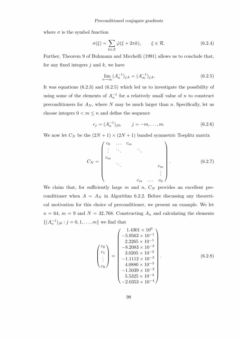
Preconditioned conjugate gradients
where σ is the symbol function
σ(ξ) =∑
k∈Z
ϕ(ξ + 2πk), ξ ∈ R. (6.2.4)
Further, Theorem 9 of Buhmann and Micchelli (1991) allows us to conclude that,
for any fixed integers j and k, we have
limn→∞
(A−1n )j,k = (A−1
∞ )j,k. (6.2.5)
It was equations (6.2.3) and (6.2.5) which led us to investigate the possibility of
using some of the elements of A−1n for a relatively small value of n to construct
preconditioners for AN , where N may be much larger than n. Specifically, let us
choose integers 0 < m ≤ n and define the sequence
cj = (A−1n )j0, j = −m, . . . ,m. (6.2.6)
We now let CN be the (2N + 1) × (2N + 1) banded symmetric Toeplitz matrix
CN =
c0 . . . cm...
. . .. . .
cm
. . . cm...
cm . . . c0
. (6.2.7)
We claim that, for sufficiently large m and n, CN provides an excellent pre-
conditioner when A = AN in Algorithm 6.2.2. Before discussing any theoreti-
cal motivation for this choice of preconditioner, we present an example. We let
n = 64, m = 9 and N = 32, 768. Constructing An and calculating the elements
(A−1n )j0 : j = 0, 1, . . . ,m we find that
c0
c1...c9
=
1.4301 × 100
−5.9563 × 10⁻¹
2.2265 × 10⁻¹
−8.2083 × 10⁻²
3.0205 × 10⁻²
−1.1112 × 10⁻²
4.0880 × 10⁻³
−1.5039 × 10⁻³
5.5325 × 10⁻⁴
−2.0353 × 10⁻⁴
. (6.2.8)
98
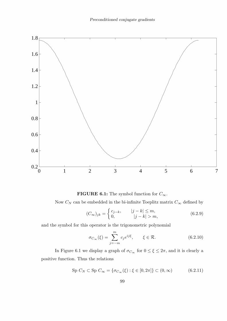
Preconditioned conjugate gradients
0.2
0.4
0.6
0.8
1
1.2
1.4
1.6
1.8
0 1 2 3 4 5 6 7
FIGURE 6.1: The symbol function for C∞.
Now CN can be embedded in the bi-infinite Toeplitz matrix C∞ defined by
(C∞)jk =
cj−k, |j − k| ≤ m,0, |j − k| > m,
(6.2.9)
and the symbol for this operator is the trigonometric polynomial
σC∞(ξ) =
m∑
j=−m
cjeijξ, ξ ∈ R. (6.2.10)
In Figure 6.1 we display a graph of σC∞for 0 ≤ ξ ≤ 2π, and it is clearly a
positive function. Thus the relations
Sp CN ⊂ Sp C∞ = σC∞(ξ) : ξ ∈ [0, 2π] ⊂ (0,∞) (6.2.11)
99

Preconditioned conjugate gradients
imply that CN is positive definite. Hence it is suitable to use CN as the precon-
ditioner in Algorithm 6.2.2. Our aim in this example is to compare this choice
of preconditioner with the use of the identity matrix as the preconditioner. To
this end, we let the elements of the righthandside vector b of Algorithm 6.2.2 be
random real numbers uniformly distributed in the interval [−1, 1]. Applying Al-
gorithm 6.2.2 using the identity matrix as the preconditioner provides the results
of Table 6.1. Table 6.2 contains the analogous results using (6.2.7) and (6.2.8).
In both cases the iterations were stopped when the residual vector satisfied the
bound ‖rk+1‖/‖b‖ < 10−13. The behaviour shown in the tables is typical; we find
that the number of steps required is independent of N and b.
Iteration Error
1 2.797904 × 101
10 1.214777 × 10⁻²
20 1.886333 × 10⁻⁶
30 2.945903 × 10⁻¹⁰
33 2.144110 × 10⁻¹¹
34 8.935534 × 10⁻¹²
Table 6.1: No preconditioning
Iteration Error
1 2.315776 × 10⁻¹
2 1.915017 × 10⁻³
3 1.514617 × 10⁻⁷
4 1.365228 × 10⁻¹¹
5 1.716123 × 10⁻¹⁵
Table 6.2: Using (6.2.7) and (6.2.8) as the preconditioner
Why should (6.2.7) and (6.2.8) provide a good preconditioner? Let us con-
sider the bi-infinite Toeplitz matrix C∞A∞. The spectrum of this operator is given
100

Preconditioned conjugate gradients
by
Sp C∞A∞ = σC∞(ξ)σ(ξ) : ξ ∈ [0, 2π], (6.2.12)
where σ is given by (6.2.4) and σC∞by (6.2.10). Therefore in order to concentrate
Sp C∞A∞ at unity we must have
σC∞(ξ)σ(ξ) ≈ 1, ξ ∈ [0, 2π]. (6.2.13)
In other words, we want σC∞to be a trigonometric polynomial approximating the
continuous function 1/σ. Now if the Fourier series of 1/σ is given by
σ−1(ξ) =∑
j∈Z
γjeijξ, ξ ∈ R, (6.2.14)
then its Fourier coefficients (γj)j∈Z are the coefficients of the cardinal function χ
for the integer grid, that is
χ(x) =∑
j∈Z
γjϕ(x − j), x ∈ R, (6.2.15)
and
χ(k) = δ0k, k ∈ Z. (6.2.16)
(See, for instance, Buhmann (1990).) Recalling (6.2.5), we deduce that one way
to calculate approximate values of the coefficients (γj)j∈Z is to solve the linear
system
Anc(n) = e0, (6.2.17)
where e0 = (δj0)nj=−n ∈ R2n+1. This observation is not new; indeed Buhmann
and Powell (1990) used precisely this idea to calculate approximate values of the
cardinal function χ. We now set
cj = c(n)j , 0 ≤ j ≤ m, (6.2.18)
and we observe that the symbol function σ for the Gaussian is a theta function
(see Section 4.2). Thus σ is a positive continuous function whose Fourier series is
absolutely convergent. Hence 1/σ is a positive continuous function and Wiener’s
101

Preconditioned conjugate gradients
lemma (Rudin (1973)) implies the absolute convergence, and therefore the uniform
convergence, of its Fourier series. We deduce that the symbol function σC∞can
be chosen to approximate 1/σ to within any required accuracy. More formally we
have the
Lemma 6.2.3. Given any ε > 0, there are positive integers m and n0 such that
∣∣∣σ(ξ)m∑
j=−m
c(n)j eijξ − 1
∣∣∣ ≤ ε, ξ ∈ [0, 2π],
for every n ≥ n0, where c(n) = (c(n)j )n
j=−n is given by (6.2.17).
Proof. The uniform convergence of the Fourier series for σ implies that we can
choose m such that
∣∣∣σ(ξ)
m∑
j=−m
γjeijξ − 1
∣∣∣ ≤ ε, ξ ∈ [0, 2π].
By (6.2.5), we can also choose n0 such that |γj − c(n)j | ≤ ε for j = −m, . . . ,m and
n ≥ n0. Then we have
∣∣∣σ(ξ)
m∑
j=−m
c(n)j eijξ − 1
∣∣∣ ≤∣∣∣σ(ξ)
m∑
j=−m
γjeijξ − 1
∣∣∣ + σ(ξ)∣∣∣
m∑
j=−m
(γj − c(n)j )eijξ|
≤ ε[1 + (2m + 1)σ(0)],
remembering from Chapter 4 that 0 < σ(π) ≤ σ(ξ) ≤ σ(0). Since ε is arbitrary
the lemma is true.
6.3. The Multiquadric
The multiquadric interpolation matrix
A =(ϕ(‖xj − xk‖)
)n
j,k=1,
where ϕ(r) = (r2 + c2)1/2 and (xj)nj=1 are points in Rd, is not positive definite.
We recall from Chapter 2 that it is almost negative definite, that is for any real
numbers (yj)nj=1 satisfying
∑yj = 0 we have
n∑
j,k=1
yjykϕ(‖xj − xk‖) ≤ 0. (6.3.1)
102
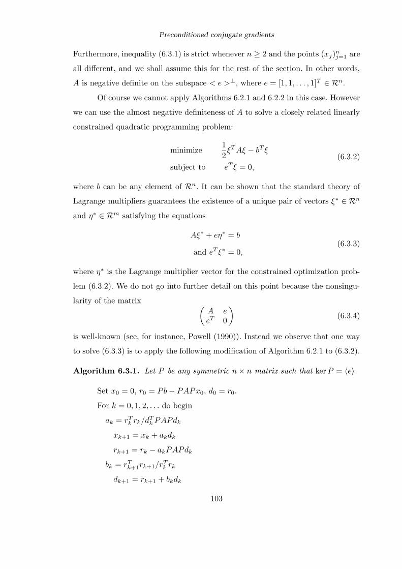
Preconditioned conjugate gradients
Furthermore, inequality (6.3.1) is strict whenever n ≥ 2 and the points (xj)nj=1 are
all different, and we shall assume this for the rest of the section. In other words,
A is negative definite on the subspace < e >⊥, where e = [1, 1, . . . , 1]T ∈ Rn.
Of course we cannot apply Algorithms 6.2.1 and 6.2.2 in this case. However
we can use the almost negative definiteness of A to solve a closely related linearly
constrained quadratic programming problem:
minimize1
2ξT Aξ − bT ξ
subject to eT ξ = 0,
(6.3.2)
where b can be any element of Rn. It can be shown that the standard theory of
Lagrange multipliers guarantees the existence of a unique pair of vectors ξ∗ ∈ Rn
and η∗ ∈ Rm satisfying the equations
Aξ∗ + eη∗ = b
and eT ξ∗ = 0,(6.3.3)
where η∗ is the Lagrange multiplier vector for the constrained optimization prob-
lem (6.3.2). We do not go into further detail on this point because the nonsingu-
larity of the matrix (A eeT 0
)(6.3.4)
is well-known (see, for instance, Powell (1990)). Instead we observe that one way
to solve (6.3.3) is to apply the following modification of Algorithm 6.2.1 to (6.3.2).
Algorithm 6.3.1. Let P be any symmetric n × n matrix such that ker P = 〈e〉.
Set x0 = 0, r0 = Pb − PAPx0, d0 = r0.
For k = 0, 1, 2, . . . do begin
ak = rTk rk/dT
k PAPdk
xk+1 = xk + akdk
rk+1 = rk − akPAPdk
bk = rTk+1rk+1/rT
k rk
dk+1 = rk+1 + bkdk
103

Preconditioned conjugate gradients
Stop if ‖rk+1‖ or ‖dk+1‖ is sufficiently small.
end.
We observe that Algorithm 6.3.1 solves the linearly constrained optimiza-
tion problem
minimize1
2xT PAPx − bT Px
subject to eT x = 0.
(6.3.5)
Moreover, the following elementary lemma implies that the solutions ξ∗of (6.3.3)
and x∗ of (6.3.5) are related by the equations ξ∗ = Px∗.
Lemma 6.3.2. Let S be any symmetric n × n matrix and let K = ker S. The
S : K⊥ → K⊥ is a bijection. In other words, given any b ∈ K⊥ there is precisely
one a ∈ K⊥ such that
Sa = b. (6.3.6)
Proof. For any n × n matrix M we have the equation
Rn = ker M ⊕ Im MT .
Consequently the symmetric matrix S satisfies
Rn = ker S ⊕ Im S,
whence Im S = K⊥. Hence for every b ∈ K⊥ there exists α ∈ Rn such that
Sα = b. Now we can write α = a + β, where a ∈ K⊥ and β ∈ K are uniquely
determined by α. Thus Sa = Sα = b, and (6.3.6) has a solution. If a′ ∈ K⊥ also
satifies (6.3.6), then their difference a − a′ lies in the intersection K ∩ K⊥ = 0,which settles the uniqeuness of a.
Setting P = S and K = 〈e〉 in Lemma 6.3.2 we deduce that there is exactly
one x∗ ∈ 〈e〉⊥ such that
PAPx∗ = Pb,
and PAP is negative definite when restricted to the subspace 〈e〉⊥. Follwing the
development of Section 6.2, we define
C = P 2, ξk = Pxk, and δk = Pdk, (6.3.7)
104

Preconditioned conjugate gradients
as in equation (6.2.1). However we cannot define ρk by (6.2.1) because P is singular.
One solution, advocated by Dyn, Levin and Rippa (1986), is to use the recurrence
for (ρk) embodied in Algorithm 6.2.1 without further ado.
105

Preconditioned conjugate gradients
Algorithm 6.3.3a. Choose any ξ0 in 〈e〉⊥. Set ρ0 = b − Aξ0 and δ0 = Cρ0.
For k = 0, 1, 2, . . . do begin
ak = ρTk Cρk/δT
k Aδk
ξk+1 = ξk + akδk
ρk+1 = ρk − akAδk
bk = ρTk+1Cρk+1/ρT
k Cρk
δk+1 = Cρk+1 + bkδk
Stop if ‖ρk+1‖ or ‖δk+1‖ is sufficiently small.
end.
However this algorithm is unstable in finite precision arithmetic, as we shall
see in our main example below. One modification that sucessfully avoids instability
is to force the condition
ρk ∈ 〈e〉⊥, (6.3.8)
to hold for all k. Now Lemma 6.3.2 implies the existence of exactly one vector ρk ∈〈e〉⊥ for which Pρk = rk. Therefore, defining Q to be the orthogonal projection
onto 〈e〉⊥, that is Q : x 7→ x − e(eT x)/(eT e), we obtain
Algorithm 6.3.3b. Choose any ξ0 in 〈e〉⊥. Set ρ0 = Q(b − Aξ0), δ0 = Cρ0.
For k = 0, 1, 2, . . . do begin
ak = ρTk Cρk/δT
k Aδk
ξk+1 = ξk + akδk
ρk+1 = Q(ρk − akAδk)
bk = ρTk+1Cρk+1/ρT
k Cρk
δk+1 = Cρk+1 + bkδk
Stop if ‖ρk+1‖ or ‖δk+1‖ is sufficiently small.
end.
We see that the only restriction on C is that it must be a non-negative
definite symmetric matrix such that ker C = 〈e〉. It is easy to construct such a
106
Preconditioned conjugate gradients
matrix given a positive definite symmetric matrix D by adding a rank one matrix:
C = D − (De)(De)T
eT De. (6.3.9)
The Cauchy-Schwarz inequality implies that xT Cx ≥ 0 with equality if and only
if x ∈ 〈e〉. Of course we do not need to form C explicitly, since C : x 7→ Dx −(eT Dx/eT De)De. Before constructing D we consider the spectral properties of
A∞ = (ϕ(j − k))j,k∈Z in more detail.
A minor modification to Proposition 5.2.2 yields the following useful result.
We recall the definition of a zero-summing sequence from Definition 4.3.1 and that
of the symbol function from (5.2.7).
Proposition 6.3.4. For every η ∈ (0, 2π) we can find a set (y(n)j )j∈Z : n =
1, 2, . . . of zero-summing sequences such that
limn→∞
∑
j,k∈Z
y(n)j y
(n)k ϕ(j − k)
/∑
j∈Z
[y(n)j ]2 = σ(η). (6.3.10)
Proof. We adopt the proof technique of Proposition 5.2.2. For each positive integer
n we define the trigonometric polynomial
Ln(ξ) = n−1/2n−1∑
k=0
eikξ, ξ ∈ R,
and we recall from Section 4.2 that
Kn(ξ) =sin2 nξ/2
n sin2 ξ/2= |Ln(ξ)|2 , (6.3.11)
where Kn is the nth degree Fejer kernel. We now choose (y(n)j )j∈Z to be the Fourier
coefficients of the trigonometric polynomial ξ 7→ Ln(ξ − η) sin ξ/2, which implies
the relation ∣∣∣∑
j∈Z
y(n)j eijξ
∣∣∣2
= sin2 ξ/2 Kn(ξ − η),
and we see that (y(n)j )j∈Z is a zero-summing sequence. By the Parseval relation
we have∑
j∈Z
[y(n)j ]2 = (2π)−1
∫ 2π
0
sin2 ξ/2 Kn(ξ − η) dξ (6.3.12)
107

Preconditioned conjugate gradients
and the approximate identity property of the Fejer kernel (Zygmund (1988), p.
86) implies that
sin2 η/2 = limn→∞
(2π)−1
∫ 2π
0
sin2 ξ/2 Kn(ξ − η) dξ
= limn→∞
∑
j∈Z
[y(n)j ]2.
Further, because σ is continuous on (0, 2π) (see Section 4.4), we have
sin2 η/2 σ(η) = limn→∞
(2π)−1
∫ 2π
0
sin2 ξ/2 Kn(ξ − η)σ(ξ) dξ
= limn→∞
∑
j,k∈Z
y(n)j y
(n)k ϕ(j − k),
the last line being a consequence of (4.3.6).
Thus we have shown that, just as in the classical theory of Toeplitz op-
erators (Grenander and Szego (1984)), everything depends on the range of val-
ues of the symbol function σ. Because σ inherits the double pole that ϕ enjoys
at zero, we have σ: (0, 2π) 7→ (σ(π),∞). In Figure 6.2 we display the function
[0, 2π] 3 ξ 7→ 1/σ(ξ).
Now let m be a positive integer and let (dj)mj=−m be an even sequence of
real numbers. We define a bi-infinite banded symmetric Toeplitz matrix D∞ by
the equations
(D∞)jk =
dj−k, |j − k| ≤ m,0, otherwise .
(6.3.13)
Thus (D∞A∞)jk = ψ(j − k) where ψ(x) =∑m
l=−m dlϕ(x − l). Further
∑
j,k∈Z
yjykψ(j − k) = (2π)−1
∫ 2π
0
∣∣∣∑
j∈Z
yjeijξ
∣∣∣2
σD∞(ξ)σ(ξ) dξ. (6.3.14)
Now the function ξ 7→ σD∞(ξ)σ(ξ) is continuous for ξ ∈ (0, 2π), so the argument
of Proposition 6.3.4 also shows that, for every η ∈ (0, 2π), we can find a set
(y(n)j )j∈Z : n = 1, 2, . . . of zero-summing sequences such that
limn→∞
∑
j,k∈Z
y(n)j y
(n)k ψ(j − k)
/∑
j∈Z
[y(n)j ]2 = σD∞
(η)σ(η). (6.3.15)
108

Preconditioned conjugate gradients
0
5
10
15
20
25
0 1 2 3 4 5 6 7
Figure 6.2: The reciprocal symbol function 1/σ for the multiquadric.
A good preconditioner must ensure that σD∞(ξ)σ(ξ) : ξ ∈ (0, 2π) is a
bounded set. Because of the form of σD∞we have the equation
m∑
j=−m
dj = 0. (6.3.16)
Moreover, as in Section 6.2, we want the approximation
σD∞(ξ)σ(ξ) ≈ 1, ξ ∈ (0, 2π), (6.3.17)
and we need σD∞to be a non-negative trigonometric polynomial which is positive
almost everywhere, which ensures that every one of its principal minors is positive
definite.
109
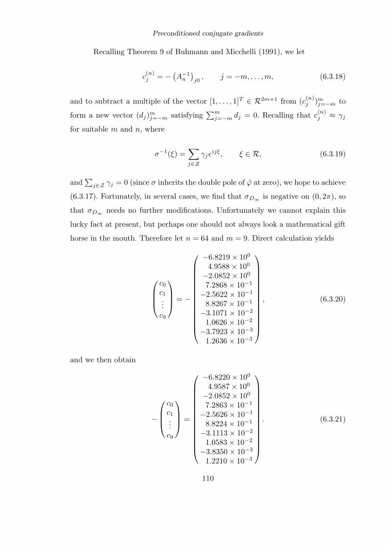
Preconditioned conjugate gradients
Recalling Theorem 9 of Buhmann and Micchelli (1991), we let
c(n)j = −
(A−1
n
)j0
, j = −m, . . . ,m, (6.3.18)
and to subtract a multiple of the vector [1, . . . , 1]T ∈ R2m+1 from (c(n)j )m
j=−m to
form a new vector (dj)mj=−m satisfying
∑mj=−m dj = 0. Recalling that c
(n)j ≈ γj
for suitable m and n, where
σ−1(ξ) =∑
j∈Z
γjeijξ, ξ ∈ R, (6.3.19)
and∑
j∈Z γj = 0 (since σ inherits the double pole of ϕ at zero), we hope to achieve
(6.3.17). Fortunately, in several cases, we find that σD∞is negative on (0, 2π), so
that σD∞needs no further modifications. Unfortunately we cannot explain this
lucky fact at present, but perhaps one should not always look a mathematical gift
horse in the mouth. Therefore let n = 64 and m = 9. Direct calculation yields
c0
c1...c9
= −
−6.8219 × 100
4.9588 × 100
−2.0852 × 100
7.2868 × 10⁻¹
−2.5622 × 10⁻¹
8.8267 × 10⁻¹
−3.1071 × 10⁻²
1.0626 × 10⁻²
−3.7923 × 10⁻³
1.2636 × 10⁻³
, (6.3.20)
and we then obtain
−
c0
c1...c9
=
−6.8220 × 100
4.9587 × 100
−2.0852 × 100
7.2863 × 10⁻¹
−2.5626 × 10⁻¹
8.8224 × 10⁻¹
−3.1113 × 10⁻²
1.0583 × 10⁻²
−3.8350 × 10⁻³
1.2210 × 10⁻³
. (6.3.21)
110

Preconditioned conjugate gradients
Figures 6.3 and 6.4 display the functions σD∞and ξ 7→ σD∞
(ξ)/ sin2(ξ/2) on the
domain [0, 2π] respectively. The latter is clearly a positive function, which implies
that the former is positive on the open interval (0, 2π).
Thus, given
AN =(ϕ(j − k)
)N
j,k=−N
for any N ≥ n, we let DN be any (2N + 1)× (2N + 1) principal minor of D∞ and
define the preconditioner CN by the equation
CN = DN − (DNe)(DNe)T
eT DNe, (6.3.22)
where e = [1, . . . , 1]T ∈ R2N+1. We reiterate that we actually compute the matrix-
vector product CNx by the operations x 7→ DNx− (eT DNx/eT DNe)e rather than
by storing the elements of CN in memory.
CN provides an excellent preconditioner. Tables 6.3 and 6.4 illustrate its
use when Algorithm 6.3.3b is applied to the linear system
ANx + ey = b,
eT x = 0,(6.3.23)
when N = 2, 048 and N = 32, 768 respectively. Here y ∈ R, e = [1, . . . , 1]T ∈R2N+1 and b ∈ R2N+1 consists of pseudo-random real numbers uniformly dis-
tributed in the interval [−1, 1]. Again, this behaviour is typical and all our numer-
ical experiments indicate that the number of steps is independent of N . We remind
the reader that the error shown is ‖ρk+1‖, but that the iterations are stopped when
either ‖ρk+1‖ or ‖δk+1‖ is less than 10−13‖b‖, where we are using the notation of
Algorithm 6.3.3b.
It is interesting to compare Table 6.3 with Table 6.5. Here we have chosen
m = 1, and the preconditioner is essentially a multiple of the second divided
difference preconditioner advocated by Dyn, Levin and Rippa (1986). Indeed, we
find that d0 = 7.8538 and d1 = d−1 = −3.9269. We see that its behaviour is clearly
inferior to the preconditioner generated by choosing m = 9. Furthermore, this is
to be expected, because we are choosing a smaller finite section to approximate
111

Preconditioned conjugate gradients
the reciprocal of the symbol function. However, because σD∞(ξ) is a multiple of
sin2 ξ/2, this preconditioner still possesses the property that σD∞(ξ)σ(ξ) : ξ ∈
(0, 2π) is a bounded set of real numbers.
Iteration Error
1 3.975553 × 10⁴
2 8.703344 × 10⁻¹
3 2.463390 × 10⁻²
4 8.741920 × 10⁻³
5 3.650521 × 10⁻⁴
6 5.029770 × 10⁻⁶
7 1.204610 × 10⁻⁵
8 1.141872 × 10⁻⁷
9 1.872273 × 10⁻⁹
10 1.197310 × 10⁻⁹
11 3.103685 × 10⁻¹¹
Table 6.3: Preconditioned CG – m = 9, n = 64, N = 2, 048
Iteration Error
1 2.103778 × 10⁵
2 4.287497 × 100
3 5.163441 × 10⁻¹
4 1.010665 × 10⁻¹
5 1.845113 × 10⁻³
6 3.404016 × 10⁻³
7 3.341912 × 10⁻⁵
8 6.523212 × 10⁻⁷
9 1.677274 × 10⁻⁵
10 1.035225 × 10⁻⁸
11 1.900395 × 10⁻¹⁰
Table 6.4: Preconditioned CG – m = 9, n = 64, N = 32, 768
112
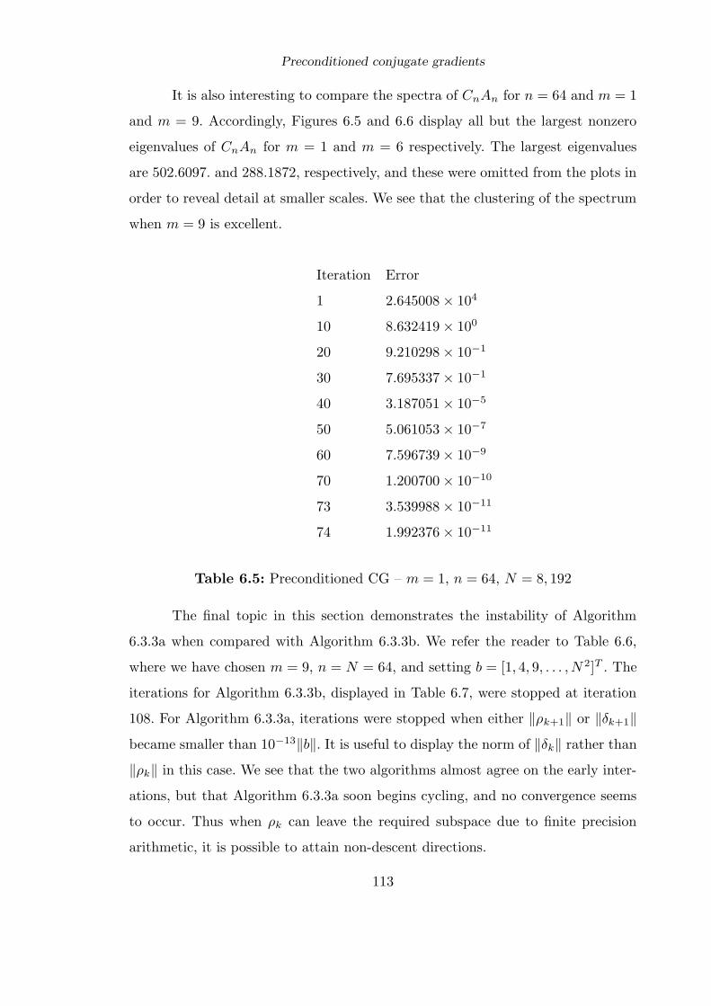
Preconditioned conjugate gradients
It is also interesting to compare the spectra of CnAn for n = 64 and m = 1
and m = 9. Accordingly, Figures 6.5 and 6.6 display all but the largest nonzero
eigenvalues of CnAn for m = 1 and m = 6 respectively. The largest eigenvalues
are 502.6097. and 288.1872, respectively, and these were omitted from the plots in
order to reveal detail at smaller scales. We see that the clustering of the spectrum
when m = 9 is excellent.
Iteration Error
1 2.645008 × 10⁴
10 8.632419 × 100
20 9.210298 × 10⁻¹
30 7.695337 × 10⁻¹
40 3.187051 × 10⁻⁵
50 5.061053 × 10⁻⁷
60 7.596739 × 10⁻⁹
70 1.200700 × 10⁻¹⁰
73 3.539988 × 10⁻¹¹
74 1.992376 × 10⁻¹¹
Table 6.5: Preconditioned CG – m = 1, n = 64, N = 8, 192
The final topic in this section demonstrates the instability of Algorithm
6.3.3a when compared with Algorithm 6.3.3b. We refer the reader to Table 6.6,
where we have chosen m = 9, n = N = 64, and setting b = [1, 4, 9, . . . , N 2]T . The
iterations for Algorithm 6.3.3b, displayed in Table 6.7, were stopped at iteration
108. For Algorithm 6.3.3a, iterations were stopped when either ‖ρk+1‖ or ‖δk+1‖became smaller than 10−13‖b‖. It is useful to display the norm of ‖δk‖ rather than
‖ρk‖ in this case. We see that the two algorithms almost agree on the early inter-
ations, but that Algorithm 6.3.3a soon begins cycling, and no convergence seems
to occur. Thus when ρk can leave the required subspace due to finite precision
arithmetic, it is possible to attain non-descent directions.
113
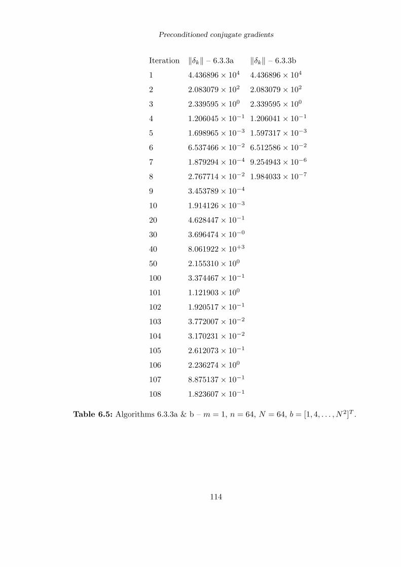
Preconditioned conjugate gradients
Iteration ‖δk‖ – 6.3.3a ‖δk‖ – 6.3.3b
1 4.436896 × 10⁴ 4.436896 × 10⁴
2 2.083079 × 10² 2.083079 × 10²
3 2.339595 × 100 2.339595 × 100
4 1.206045 × 10⁻¹ 1.206041 × 10⁻¹
5 1.698965 × 10⁻³ 1.597317 × 10⁻³
6 6.537466 × 10⁻² 6.512586 × 10⁻²
7 1.879294 × 10⁻⁴ 9.254943 × 10⁻⁶
8 2.767714 × 10⁻² 1.984033 × 10⁻⁷
9 3.453789 × 10⁻⁴
10 1.914126 × 10⁻³
20 4.628447 × 10⁻¹
30 3.696474 × 10−0
40 8.061922 × 10+3
50 2.155310 × 100
100 3.374467 × 10⁻¹
101 1.121903 × 100
102 1.920517 × 10⁻¹
103 3.772007 × 10⁻²
104 3.170231 × 10⁻²
105 2.612073 × 10⁻¹
106 2.236274 × 100
107 8.875137 × 10⁻¹
108 1.823607 × 10⁻¹
Table 6.5: Algorithms 6.3.3a & b – m = 1, n = 64, N = 64, b = [1, 4, . . . , N 2]T .
114

Preconditioned conjugate gradients
0
5
10
15
20
25
0 1 2 3 4 5 6 7
Figure 6.3: The function σD∞.
115

Preconditioned conjugate gradients
0
5
10
15
20
25
0 1 2 3 4 5 6 7
Figure 6.4: The function ξ 7→ σD∞(ξ)/ sin2(ξ/2).
116

Preconditioned conjugate gradients
0
1
2
3
4
5
6
7
8
0 20 40 60 80 100 120 140
ooooooooooooooooooooooooo
ooooooooooo
oooooooo
oooooo
oooooo
oooooo
oooo
oooo
oooo
oooo
oooo
oooo
oooo
oooo
oooo
oooo
oooo
oooo
oooo
oooo
ooooo
ooo
Figure 6.5: The spectrum of CnAn for m = 1 and n = 64.
117
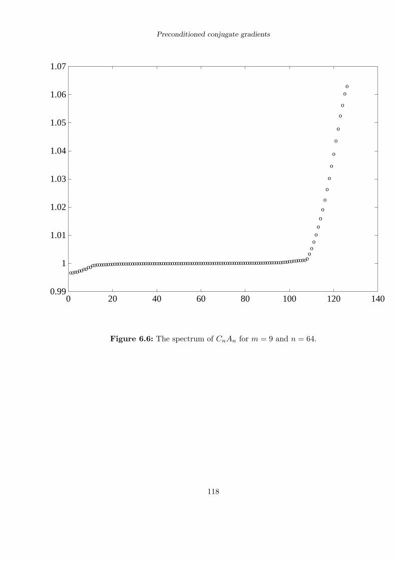
Preconditioned conjugate gradients
0.99
1
1.01
1.02
1.03
1.04
1.05
1.06
1.07
0 20 40 60 80 100 120 140
oooooooooo
oooooooooooooooooooooooooooooooooooooooooooooooooooooooooooooooooooooooooooooooooooooooooooooooooo
oooooo
o
o
o
o
o
o
o
o
o
o
oo
Figure 6.6: The spectrum of CnAn for m = 9 and n = 64.
118
On the asymptotic cardinal function for the multiquadric
7 : On the asymptotic cardinal function for the multiquadric
7.1. Introduction
The radial basis function approach to interpolating a function f :Rd → R on the
integer lattice Zd is as follows. Given a continuous univariate function ϕ: [0,∞) →R, we seek a cardinal function
χ(x) =∑
j∈Zd
ajϕ(‖x − j‖), x ∈ Rd, (7.1.1)
that satisfies
χ(k) = δ0,k, k ∈ Zd.
Therefore
If(x) =∑
j∈Zd
f(j)χ(x − j), x ∈ Rd, (7.1.2)
is an interpolant to f on the integer lattice whenever (7.1.2) is well defined. Here
‖ · ‖ is the Euclidean norm on Rd. This approach provides a useful and flexible
family of approximants for many choices of ϕ, but here we concentrate on the
Hardy multiquadric ϕc(r) = (r2 + c2)1/2. For this function, Buhmann (1990) has
shown that a cardinal function χc exists and its Fourier tranform is given by the
equation
χc(ξ) =ϕc(‖ξ‖)∑
k∈Zd ϕc(‖ξ + 2πk‖) , ξ ∈ Rd, (7.1.3)
where ϕc(‖ξ‖) : ξ ∈ Rd is the generalized Fourier transform of ϕc(‖x‖) :
x ∈ Rd. Further, χc possesses a classical Fourier transform (see Jones (1982) or
Schwartz (1966)). In this chapter, we prove that χc enjoys the following property:
limc→∞
χc(ξ) =
1, ξ ∈ (−π, π)d,0, ξ /∈ [−π, π]d,
(7.1.4)
which sheds new light on the approximation properties of the multiquadric as c →∞. For example, in the case d = 1, (7.1.4) implies that limc→∞ χc(x) = sinc(x),
providing a perhaps unexpected link with sampling theory and the classical theory
of the Whittaker cardinal spline. Further, our work has links with the error analysis
119

On the asymptotic cardinal function for the multiquadric
of Buhmann and Dyn (1991) and illuminates the explicit calculation of Section 4
of Powell (1991). It may also be compared with the results of Madych and Nelson
(1990) and Madych (1990), because these papers present analogous results for
polyharmonic cardinal splines.
7.2. Some properties of the multiquadric
The generalized Fourier transform of ϕc is given by
ϕc(‖ξ‖) = −π−1(2πc/‖ξ‖)(d+1)/2K(d+1)/2(c‖ξ‖), (7.2.1)
for nonzero ξ ∈ Rd (see Jones (1982)). Here Kν(r) : r > 0 are the modified
Bessel functions, which are positive and smooth in R+, have a pole at the origin,
and decay exponentially (see Abramowitz and Stegun (1970)). There is an integral
representation for these modified Bessel functions (Abramowitz and Stegun (1970),
equation 9.6.23) which transforms (7.2.1) into a highly useful formula for ϕc:
ϕc(‖ξ‖) = −λdcd+1
∫ ∞
1
exp(−cx‖ξ‖)(x2 − 1)d/2 dx, (7.2.2)
where λd = πd/2/Γ(1 + d/2). A simple consequence of (7.2.2) is the following
lemma, which bounds the exponential decay of ϕc.
Lemma 7.2.1. If ‖ξ‖ > ‖η‖ > 0, then
|ϕc(‖ξ‖)| ≤ exp[−c(‖ξ‖ − ‖η‖)] |ϕc(‖η‖)|.
Proof. Applying (7.2.2), we obtain
|ϕc(‖ξ‖)| = λdcd+1
∫ ∞
1
exp[−cx(‖ξ‖ − ‖η‖)] exp(−cx‖η‖) (x2 − 1)d/2 dx
≤ exp(−c(‖ξ‖ − ‖η‖)) |ϕc(‖η‖)|,
providing the desired bound.
We now prove our main result. We let I:Rd → R be the characteristic
function of the cube [−π, π]d, that is
I(ξ) =
1, ξ ∈ [−π, π]d,0, ξ /∈ [−π, π]d.
120
On the asymptotic cardinal function for the multiquadric
Proposition 7.2.2. Let ξ be any fixed point of Rd. We have
limc→∞
χc(ξ) = I(ξ),
if ‖ξ‖∞ 6= π, that is ξ does not lie in the boundary of [−π, π]d.
Proof. First, suppose that ξ /∈ [−π, π]d. Then there exists a nonzero integer k0
such that ‖ξ + 2πk0‖ < ‖ξ‖, and Lemma 7.2.1 provides the bounds
|ϕc(‖ξ‖)| ≤ exp[−c(‖ξ‖ − ‖ξ + 2πk0‖)]|ϕc(‖ξ + 2πk0‖)|
≤ exp[−c(‖ξ‖ − ‖ξ + 2πk0‖)]∑
k∈Zd
|ϕc(‖ξ + 2πk‖)|.
Thus, applying (7.1.3) and remembering that ϕc does not change sign, we have
0 ≤ χc(ξ) ≤ exp[−c(‖ξ‖ − ‖ξ + 2πk0‖)], ξ /∈ [−π, π]d. (7.2.3)
The upper bound of (7.2.3) converges to zero as c → ∞, which completes the proof
for this range of ξ.
Suppose now that ξ ∈ (−π, π)d. Further, we shall assume that ξ is nonzero,
because we know that χc(0) = 1 for all values of c. Then ‖ξ + 2πk‖ > ‖ξ‖, for
every nonzero integer k ∈ Zd. Now (7.1.3) provides the expression
χc(ξ) =(1 +
∑
k∈Zd\0
∣∣∣ ϕc(‖ξ + 2πk‖)ϕc(‖ξ‖)
∣∣∣)−1
. (7.2.4)
We shall show that
limc→∞
∑
k∈Zd\0
∣∣∣∣ϕc(‖ξ + 2πk‖)
ϕc(‖ξ‖)
∣∣∣∣ = 0, ξ ∈ (−π, π)d, (7.2.5)
which, together with (7.2.4), implies that limc→∞ χc(ξ) = 1.
Now Lemma 7.2.1 implies that
∑
k∈Zd\0
∣∣∣∣ϕc(‖ξ + 2πk‖)
ϕc(‖ξ‖)
∣∣∣∣ ≤∑
k∈Zd\0
exp[−c(‖ξ + 2πk‖ − ‖ξ‖)], (7.2.6)
121

On the asymptotic cardinal function for the multiquadric
and each term of the series on the right converges to zero as c → ∞, since ‖ξ +
2πk‖ > ‖ξ‖ for every nonzero integer k. Therefore we need only deal with the tail
of the series. Specifically, we derive the equation
limc→∞
∑
‖k‖≥2‖e‖
exp[−c(‖ξ + 2πk‖ − ‖ξ‖)] = 0, (7.2.7)
where e = [1, 1, . . . , 1]T . Now, if ‖k‖ ≥ 2‖e‖, then
‖ξ + 2πk‖ − ‖ξ‖ ≥ 2π(‖k‖ − ‖e‖) ≥ π‖k‖,
remembering that we have ‖ξ‖ ≤ π‖e‖. Hence
∑
‖k‖≥2‖e‖
exp[−c(‖ξ + 2πk‖ − ‖ξ‖)] ≤∑
‖k‖≥2‖e‖
exp(−πc‖k‖). (7.2.8)
It is a simple exercise to prove that the series∑
‖k‖≥2‖e‖ exp(−π‖k‖) is convergent.
Therefore, given any ε > 0, there exists a positive number R ≥ 1 such that
∑
‖k‖≥2R‖e‖
exp(−π‖k‖) ≤ ε.
Consequently, when c ≥ dRe we have the inequality
∑
‖k‖≥2‖e‖
exp(−πc‖k‖) ≤∑
‖k‖≥2R‖e‖
exp(−π‖k‖) ≤ ε,
which establishes (7.2.5). The proof is complete.
7.3. Multiquadrics and entire functions of exponential type π
Definition 7.3.1 Let f ∈ L2(Rd). We shall say that f is a function of exponential
type A if its Fourier transform f is supported by the cube [−A,A]d. We shall denote
the set of all functions of exponential type A by EA(Rd).
We remark that the Paley-Wiener theorem implies that f may be extended
to an entire function on Cd satisfying a certain growth condition at infinity (see
Stein and Weiss (1971), pages 108ff), although we do not need this result.
122
On the asymptotic cardinal function for the multiquadric
Lemma 7.3.2. Let f ∈ Eπ(Rd)∩L2(Rd) be a continuous function. Then we have
the equation∑
k∈Zd
f(ξ + 2πk) =∑
k∈Zd
f(k) exp(−ikξ), (7.3.1)
the second series being convergent in L2(Rd).
Proof. Let
g(ξ) =∑
k∈Zd
f(ξ + 2πk), ξ ∈ Rd.
At any point ξ ∈ Rd, this series contains at most one nonzero term, because of
the condition on the support of f . Hence g is well defined. Further, we have the
relations ∫
[−π,π]d|g(ξ)|2 dξ =
∫
Rd
|f(ξ)|2 dξ < ∞,
since the Parseval theorem implies that f is an element of L2(Rd). Thus g ∈L2([−π, π]d) and its Fourier series
g(ξ) =∑
k∈Zd
gk exp(ikξ),
is convergent in L2([−π, π]d). The Fourier coefficients are given by the expressions
gk = (2π)−d
∫
[−π,π]df(ξ) exp(−ikξ) dξ = (2π)−d
∫
Rd
f(ξ) exp(−ikξ) dξ = f(−k),
where the final equation uses the Fourier inversion theorem for L2(Rd). The proof
is complete.
We observe that an immediate consequence of the lemma is the convergence
of the series∑
k∈Zd [f(k)]2, by the Parseval theorem.
For the following results, we shall need the fact that χc ∈ L2(Rd), which is
a consequence of the analysis of Buhmann (1990).
Lemma 7.3.3. Let f ∈ Eπ(Rd) ∩ L2(Rd) be a continuous function. For each
positive integer n, we define the function
Snc f(ξ) =
∑
‖k‖1≤n
f(k) exp(−ikξ)
χc(ξ), ξ ∈ Rd. (7.3.2)
Then Snc f : n = 1, 2, . . . forms a Cauchy sequence in L2(Rd).
123
On the asymptotic cardinal function for the multiquadric
Proof. Let Qn:Rd → R be the trigonometric polynomial
Qn(ξ) =∑
‖k‖1≤n
f(k) exp(−ikξ), (7.3.3)
so that Snc f(ξ) = Qn(ξ)χc(ξ). It is a consequence of Lemma 7.3.2 that this se-
quence of functions forms a Cauchy sequence in L2([−π, π]d). Indeed, we shall
prove that for m ≥ n we have
‖Smc f − Sn
c f‖L2(Rd) ≤ ‖Qm − Qn‖L2([−π,π]d), (7.3.4)
so that the sequence of functions Snc f : n = 1, 2, . . . is a Cauchy sequence in
L2(Rd).
Now Fubini’s theorem provides the relation
‖Smc f − Sn
c f‖2L2(Rd) =
∫
Rd
|Qm(ξ) − Qn(ξ)|2 χ2c(ξ) dξ
=
∫
[−π,π]d|Qm(ξ) − Qn(ξ)|2
∑
l∈Zd
χ2c(ξ + 2πl)
dξ.
(7.3.5)
However, (7.1.3) gives the bound∑
l∈Zd
χ2c(ξ + 2πl) =
∑
l∈Zd
ϕ2c(‖ξ + 2πl‖)
/(
∑
k∈Zd
ϕc(‖ξ + 2πk‖))2
≤ 1,
(7.3.6)
which, together with (7.3.5), yields inequality (7.3.4).
Thus we may define
Scf(ξ) = χc(ξ)∑
k∈Zd
f(k) exp(−ikξ), (7.3.7)
and the series is convergent in L2(Rd). Applying the inverse Fourier transform
term by term, we obtain the useful equation
Scf(x) =∑
k∈Zd
f(k)χc(x − k), x ∈ Rd.
Theorem 7.3.4. Let f ∈ Eπ(Rd) ∩ L2(Rd) be a continuous function. We have
limc→∞
Scf(x) = f(x),
and the convergence is uniform on Rd.
124
On the asymptotic cardinal function for the multiquadric
Proof. We have the equation
Scf(x) − f(x) = (2π)−d
∫
Rd
∑
k∈Zd
f(ξ + 2πk) (χc(ξ) − I(ξ)) exp(ixξ) dξ.
Thus we deduce the bound
|Scf(x) − f(x)|
≤ (2π)−d
∫
[−π,π]d|f(ξ)|
∑
k∈Zd
∣∣∣χc(ξ + 2πk) − I(ξ + 2πk)∣∣∣ dξ
= (2π)−d
∫
[−π,π]d|f(ξ)|
1 − χc(ξ) +
∑
k∈Zd\0
χc(ξ + 2πk)
dξ,
(7.3.8)
using the fact that χc is non-negative, and we observe that this upper bound is
independent of x. Therefore we prove that the upper bound converges to zero as
c → ∞.
Applying (7.1.3), we obtain the relation
∑
k∈Zd\0
χc(ξ + 2πk) = 1 − χc(ξ), (7.3.9)
whence
|Scf(x) − f(x)| ≤ 2(2π)−d
∫
[−π,π]d|f(ξ)|(1 − χc(ξ)) dξ. (7.3.10)
Now f ∈ L2([−π, π]d) implies f ∈ L1([−π, π]d), by the Cauchy-Schwartz inequal-
ity. Further, Proposition 7.2.2 gives the limit limc→∞ χc(ξ) = 1, for ξ ∈ (−π, π)d,
and we have 0 ≤ 1 − χc(ξ) ≤ 1, by (7.1.3). Therefore the dominated convergence
theorem implies that
limc→∞
(2π)−d
∫
[−π,π]d|f(ξ)|(1 − χc(ξ)) dξ = 0.
The proof is complete.
125

On the asymptotic cardinal function for the multiquadric
7.4. Discussion
Section 4 of Powell (1991) provides an explicit calculation that is analogous to the
proof of Theorem 7.3.4 when f(x) = x2. Of course, this function does not satisfy
the conditions of Theorem 7.3.4. Therefore extensions of this result are necessary,
but the final form of the theorem is not clear at present.
Theorem 7.3.4 encourages the use of large c for certain functions. Indeed,
it suggests that large c will provide high accuracy interpolants for univariate func-
tions that are well approximated by integer translates of the sinc function. Thus, in
exact arithmetic, a large value of c should be useful whenever the function is well
approximated by the Whittaker cardinal series. However, we recall that the linear
systems arising when c is large can be rather ill-conditioned. Indeed, in Chapter
4 we proved that the smallest eigenvalue of the interpolation matrix generated by
a finite regular grid converges to zero exponentially quickly as c → ∞. We refer
the reader to Table 4.1 for further information. Therefore special techniques are
required for the effective use of large c.
126
Conclusions
8 : Conclusions
There seems to be no interest in using non-Euclidean norms for radial basis
functions at present, possibly because of the poor approximation properties of
the `1-norm ‖ · ‖1 reported by several workers. Thus Chapter 2 does not seem
to have any practical applications yet. However, it may be useful to use p-norms
(1 < p < 2), or functions of p-norms, when there is a known preferred direction
in the underlying function, because radial basis functions based on the Euclidean
norm can perform poorly in this context. On a purely theoretical note, we observe
that the construction of Section 2.4 can be applied to any norm enjoying the
symmetries of the cube.
The greatest weakness – and the greatest strength – of the norm estimates
of Chapters 3–6 lies in their dependence on regular grids. However, we note that
the upper bounds on norms of inverses apply to sets of centres which can be
arbitrary subsets of a regular grid. In other words, contiguous subsets of grids are
not required. Furthermore, we conjecture that a useful upper bound on the norm
of the inverse generated by an arbitrary set of centres with minimal separation
distance δ (that is ‖xj − xk‖ ≥ δ > 0 if j 6= k) will be provided by the upper
bound for the inverse generated by a regular grid of spacing δ.
Probably the most important practical finding of this dissertation is that
the number of steps required by the conjugate gradient algorithm can be indepen-
dent of the number of centres for suitable preconditioners. We hope to discover
preconditioners with this property for arbitrary sets of centres.
The choice of constant in the multiquadric is still being investigated (see, for
instance, Kansa and Carlson (1992)). Because the approximation of band-limited
functions is of some practical importance, our findings may be highly useful. In
short, we suggest using as large a value of the constant as the condition number
allows. Hence there is some irony in our earlier discovery that the condition number
of the interpolation matrix can increase exponentially quickly as the constant
increases.
Let us conclude with the remark that radial basis functions are extremely
127

Conclusions
rich mathematical objects, and there is much left to be discovered. It is our hope
that the strands of research initiated in this thesis will enable some of these future
discoveries.
128

References
References
Abramowitz, M., and I. A. Stegun (1970), Handbook of Mathematical Functions,
Dover Publications (New York).
Ball, K. M. (1989), Invertibility of Euclidean distance matrices and radial basis
interpolation, CAT report no. 201, Texas A & M University, College Station.
Barrodale, I., M. Berkley and D. Skea (1992), “Warping digital images using thin
plate splines”, presented at the Sixth Texas International Symposium on Approx-
imation Theory (Austin, January 1992).
Baxter, B. J. C. (1991a), “Conditionally positive functions and p-norm distance
matrices”, Constr. Approx. 7, pp. 427–440.
Baxter, B. J. C. (1991b), “Norm estimates for Toeplitz distance matrices”, Report
NA16, University of Cambridge.
Baxter, B. J. C. (1992a), “Norm estimates for inverses of distance matrices”, in
Mathematical Methods in Computer Aided Geometric Design, T. Lyche and L. L.
Schumaker (eds.), Academic Press (New York), pp. 9–18.
Baxter, B. J. C. (1992b), “On the asymptotic cardinal function of the multiquadric
ϕ(r) = (r2 + c2)1/2 as c → ∞”. To appear in a special issue of An International
Journal of Computers and Mathematics with Applications.
Baxter, B. J. C. (1992c), “Norm estimates and preconditioning for conjugate gra-
dient solution of RBF linear systems”. In preparation.
Baxter, B. J. C. and C. A. Micchelli, “Norm estimates for the `2-inverses of mul-
tivariate Toeplitz matrices”. In preparation.
Beatson, R. K. and G. N. Newsam (1992), “Fast evaluation of radial basis func-
tions: 1”. To appear in a special issue of An International Journal of Computers
and Mathematics with Applications.
de Boor, C. (1987), “Multivariate approximation”, in the The State of the Art in
129

References
Numerical Analysis, A. Iserles and M. J. D. Powell (eds.), Oxford University Press
(Oxford), pp. 87–110.
Buhmann, M. D. (1990), “Multivariate cardinal interpolation with radial basis
functions”, Constr. Approx. 6, pp. 225–256.
Buhmann, M. D. and M. J. D. Powell (1990), “Radial basis function interpolation
on an infinite regular grid”, in Algorithms for Approximation II, J. C. Mason and
M. G. Cox (eds.), Chapmann and Hall (London), pp. 146–169.
Buhmann, M. D. and N. Dyn (1991), “Error estimates for multiquadric interpola-
tion”, in Curves and Surfaces, P.-J. Laurent, A. Le Mehaute, and L. L. Schumaker
(eds.), Academic Press (New York), pp. 51–58.
Buhmann, M. D. and C. A. Micchelli (1991), “Multiply monotone functions for
cardinal interpolation”, Advances in Applied Mathematics 12 , pp. 358–386.
Chui, C. K. (1988), Multivariate Splines, SIAM Regional Conference Series in
Applied Mathematics 54 (Philadelphia).
Chui, C. K. (1992), An Introduction to Wavelets, Academic Press (New York).
Davis, P. J. (1975), Interpolation and Approximation, Dover Publications (New
York).
Dahmen, W. and C. A. Micchelli (1983), “Recent progress in multivariate splines”,
in Approximation Theory IV, C. K. Chui, L. L. Schumaker and J. D. Ward (eds),
Academic Press (New York), pp. 27–121.
Duchon, J. (1975), “Fonctions-spline du type plaque mince en dimension 2”, Tech-
nical Report 231, Universite de Grenoble.
Duchon, J. (1976), “Fonctions-spline a energie invariante par rotation”, Technical
Report 27, Universite de Grenoble.
Dyn, N., W. A. Light and E. W. Cheney (1989), “Interpolation by piecewise linear
radial basis functions”, J. Approx. Theory. 59, pp. 202–223.
130
References
Dyn, N., D. Levin and S. Rippa (1986), “Numerical procedures for surface fitting
of scattered data by radial functions”, SIAM J. Sci. Stat. Comput. 7, pp. 639–659.
Dyn, N., D. Levin and S. Rippa (1990), “Data dependent triangulations for piece-
wise linear interpolation”, IMA J. of Numer. Anal. 10, pp. 137–154.
Edrei, A. (1953), “On the generating function of doubly infinite, totally positive
sequences”, Trans. Amer. Math. Soc. 74, pp. 367–383.
Fletcher, R. (1987), Practical Methods of Optimization, Wiley & Sons (Chicester).
Franke, R. (1982), “Scattered data interpolation: tests of some methods”, Math.
of Comp. 38, pp. 181–200.
Franke, R. (1987), “Recent advances in the approximation of surfaces from scat-
tered data”, in Topics in Multivariate Approximation, C. K. Chui, L. L. Schumaker
and F. I. Utreras (eds), Academic Press (New York), pp. 79–98.
Golub, G. H. and C. F. Van Loan (1989), Matrix Computations, The John Hopkins
University Press (Baltimore).
Grenander, U. and G. Szego (1984), Toeplitz Forms, Chelsea (New York).
Hardy, G. H., J. E. Littlewood and G. Polya (1952), Inequalities, Cambridge Uni-
versity Press (Cambridge).
Hayes, J. G. (1987), “Fitting surfaces to data”, in The Mathematics of Surfaces,
R. R. Martin (ed.), Oxford University Press (Oxford), pp. 17–38.
Hille, E. (1962), Analytic Function Theory, Volume II, Ginn and Co. (Waltham,
Massachusetts).
Jackson, I. R. H. (1988), Radial basis function methods for multivariable approx-
imation, Ph.D. Dissertation, University of Cambridge.
Jones, D. S. (1982), The Theory of Generalised Functions, Cambridge University
Press (Cambridge).
131

References
Kansa, E. J. and R. E. Carlson (1992), “Improved accuracy of multiquadric in-
terpolation using variable shape parameters”. To appear in a special issue of An
International Journal of Computers and Mathematics with Applications.
Karlin, S. (1968), Total Positivity, Volume I, Stanford University Press (Stanford,
California).
Katznelson, Y. (1976), An Introduction to Harmonic Analysis, Dover Publications
(New York).
Light, W. A. and E. W. Cheney (1986), Approximation Theory in Tensor Product
Spaces, Lecture Notes in Mathematics 1169, Springer Verlag (Berlin).
Madych, W. R. (1990), “Polyharmonic splines, multivariate analysis and entire
functions”, International Series of Numerical Analysis 94, pp. 205–216.
Madych, W. R. and S. A. Nelson (1990), “Polyharmonic cardinal splines”, J. Ap-
prox. Theory 60, pp. 141–156.
Micchelli, C. A. (1986), “Interpolation of scattered data: distance matrices and
conditionally positive functions”, Constr. Approx. 2, pp. 11-22.
Narcowich, F. J. and J. D. Ward (1990), “Norm estimates for inverses of scat-
tered data interpolation matrices associated with completely monotonic func-
tions”, preprint.
Narcowich, F. J. and J. D. Ward (1991), “Norms of inverses and condition numbers
of matrices associated with scattered data”, J. Approx. Theory 64, pp. 69–94.
von Neumann, J. and I. J. Schoenberg (1941), “Fourier integrals and metric ge-
ometry”, Trans. Amer. Math. Soc. 50, pp. 226–251.
Powell, M. J. D. (1981), Approximation Theory and Methods, Cambridge Univer-
sity Press (Cambridge).
Powell, M. J. D. (1991), “Univariate multiquadric interpolation: some recent re-
sults”,in Curves and Surfaces, P.-J. Laurent, A. Le Mehaute, and L. L. Schumaker
132

References
(eds.), Academic Press (New York), pp. 371–381.
Powell, M. J. D. Powell (1992), “The theory of radial basis function approximation
in 1990”, in Advances in Numerical Analysis II: Wavelets, Subdivision Algorithms
and Radial Functions, ed. W. A. Light, Oxford University Press (Oxford), pp.
105–210.
Rudin, W. (1973), Functional Analysis, McGraw Hill (London).
Schoenberg, I. J. (1935), “Remarks to Maurice Frechet’s article ‘Sur la definition
d’une classe d’espace distancies vectoriellement applicable sur l’espace d’Hilbert.’
”, Ann. of Math. 36, pp. 724-732.
Schoenberg, I. J. (1937), “On certain metric spaces arising from Euclidean space
by a change of metric and their embedding in Hilbert space”, Ann. of Math. 38,
pp. 787-793.
Schoenberg, I. J. (1938), “Metric spaces and completely monotone functions”,
Ann. of Math. 39, pp. 811-841.
Schoenberg, I. J. (1951), “On Polya frequency functions. I. The totally positive
functions and their Laplace transforms,” J. Analyse Math. 1, pp. 331–374.
Schoenberg, I. J. (1973), Cardinal Spline Interpolation, SIAM Regional Conference
Series in Applied Mathematics 12 (Philadelphia).
Schwartz, L. (1966), Theorie des Distributions, Hermann (Paris).
Stein, E. M. and G. Weiss (1971), Introduction to Fourier analysis on Euclidean
spaces, Princeton Univ. Press (Princeton, New Jersey).
Sun, X. (1990), “Norm estimates for inverses of Euclidean distance matrices”,
preprint.
Whittaker, E. T. and G. N. Watson (1927), A Course of Modern Analysis, Cam-
bridge University Press (Cambridge).
Wilkinson, J. H. (1965), The Algebraic Eigenvalue Problem, Oxford University
133

References
Press (Oxford).
Zygmund, A. (1979), Trigonometric Series, Volumes I and II, Cambridge University
Press (Cambridge).
134