orbit: optimization by radial basis … optimization by radial basis ... a previous point must be...

ORBIT: OPTIMIZATION BY RADIAL BASIS FUNCTIONINTERPOLATION IN TRUST-REGIONS∗

STEFAN M. WILD† , ROMMEL G. REGIS‡ , AND CHRISTINE A. SHOEMAKER§

Abstract. We present a new derivative-free algorithm, ORBIT, for unconstrained local op-timization of computationally expensive functions. A trust-region framework using interpolatingRadial Basis Function (RBF) models is employed. The RBF models considered often allow OR-BIT to interpolate nonlinear functions using fewer function evaluations than the polynomial modelsconsidered by present techniques. Approximation guarantees are obtained by ensuring that a sub-set of the interpolation points are sufficiently poised for linear interpolation. The RBF property ofconditional positive definiteness yields a natural method for adding additional points. We presentnumerical results on test problems to motivate the use of ORBIT when only a relatively small numberof expensive function evaluations are available. Results on two very different application problems,calibration of a watershed model and optimization of a PDE-based bioremediation plan, are alsovery encouraging and support ORBIT’s effectiveness on blackbox functions for which no specialmathematical structure is known or available.

Key words. Derivative-Free Optimization, Radial Basis Functions, Trust-Region Methods,Nonlinear Optimization.

AMS subject classifications. 65D05, 65K05, 90C30, 90C56.

1. Introduction. In this paper we address unconstrained local minimization

minx∈Rn

f(x),(1.1)

of a computationally expensive, real-valued deterministic function f assumed to becontinuous and bounded from below. While we require additional smoothness prop-erties to guarantee convergence of the algorithm presented, we assume that all deriva-tives of f are either unavailable or intractable to compute or approximate directly.

The principal motivation for the current work is optimization of complex deter-ministic computer simulations which usually entail numerically solving systems of par-tial differential equations governing underlying physical phenomena. These simulatorsoften take the form of proprietary or legacy codes which must be treated as a black-box, permitting neither insight into special structure or straightforward application ofautomatic differentiation techniques. For the purposes of this paper, we assume thatavailable parallel computing resources are devoted to parallelization within the com-putationally expensive function, and are not utilized by the optimization algorithm.We note that pattern search methods are well-suited for parallelization [11, 14].

When analytic derivatives are unavailable, one approach is to rely on a classicalfirst-order technique employing finite difference-based estimates of ∇f to solve (1.1).

∗ Citation details: Stefan M. Wild and Rommel G. Regis and Christine A. Shoemaker,

ORBIT: Optimization by Radial Basis Function Interpolation in Trust-Regions, Cornell

University, School of Operations Research and Information Engineering Technical Report

#ORIE-1459, To appear in SIAM Journal on Scientific Computing, 2008. This work wassupported by a Department of Energy Computational Science Graduate Fellowship, grant numberDE-FG02-97ER25308 and NSF grants BES-0229176 and CCF-0305583. This research was conductedusing the resources of the Cornell Theory Center, which receives funding from Cornell University,New York State, federal agencies, foundations, and corporate partners.

†School of Operations Research and Information Engineering, Cornell University, Rhodes Hall,Ithaca, NY 14853 ([email protected]).

‡Cornell Theory Center, Cornell University, Rhodes Hall, Ithaca, NY, 14853 ([email protected]).§School of Civil and Environmental Engineering and School of Operations Research and Informa-

tion Engineering, Cornell University, Hollister Hall, Ithaca, NY, 14853. ([email protected]).

1

2 S. WILD, R. REGIS, AND C. SHOEMAKER

However, in addition to potential presence of computational noise, as both the dimen-sion and computational expense of the function grows, the n + 1 function evaluationsrequired for such estimates are often better spent sampling the function elsewhere.

For their ease of implementation and ability to find global solutions, heuristics,such as genetic algorithms and simulated annealing, are often favored by engineers.However, these algorithms are often inefficient in achieving decreases in the objectivefunction given only a limited number of function evaluations.

The approach followed by our ORBIT algorithm is based on forming a surrogatemodel which is computationally simple to evaluate and possesses well-behaved deriva-tives. This surrogate model approximates the true function locally by interpolatingit at a set of sufficiently scattered data points. The surrogate model is optimized overcompact regions to generate new points which can be evaluated by the computation-ally expensive function. By using this new function value to update the model, aniterative process develops. Over the last ten years, such derivative-free trust-regionalgorithms have become increasingly popular (see for example [5, 22, 23, 24]). How-ever, they are often tailored to minimize the underlying computational complexity,as in [24], or to yield global convergence, as in [5]. In our setting we assume that thecomputational expense of function evaluation both dominates any possible internaloptimization expense and limits the number of evaluations which can be performed.

In ORBIT, we have isolated the components which we believe to be responsible forthe success of the algorithm in preliminary numerical experiments. As in the work ofPowell [25] and Oeuvray and Bierlaire [22], we form a nonlinear interpolation modelusing fewer than a quadratic (in the dimension) number of points. A so-called “fullylinear tail” is employed to guarantee that the model approximates both the functionand its gradient reasonably well, similar to the class of models considered by Conn,Scheinberg, and Vicente in [7].

To minimize computational overhead, in both [25] and [22], the number of in-terpolation points employed is fixed and hence each time a new point is evaluated,a previous point must be dropped from the interpolation set. In ORBIT, the numberof points interpolated depends on the number of nearby points available and the setof points used can vary more freely from one iteration to the next. Our method foradding additional points in a computationally stable manner relies on a property ofradial basis functions and is based on a technique from the global optimization litera-ture [2]. Our algorithmic framework works for a wide variety of radial basis functions.While we have recently established a global convergence result in [29], the focus ofthis paper is on implementation details and the success of ORBIT in practice.

1.1. Outline. We begin by providing the necessary background on trust-regionmethods and outlining the work done to date on derivative-free trust-region methodsin Section 2. In Section 3 we introduce interpolating models based on RBFs. Thecomputational details of ORBIT are outlined in Section 4. In Section 5 we introducetechniques for benchmarking optimization algorithms in the computationally expen-sive setting and provide numerical results on standard test problems. Results on twoapplications from Environmental Engineering are presented in Section 6.

2. Trust-Region Methods. We begin with a review of the trust-region frame-work upon which our algorithm relies. Trust-region methods employ a surrogatemodel mk which is assumed to approximate f within a neighborhood of the currentiterate xk. We define this so-called trust-region for an implied (center, radius) pair

ORBIT 3

(a) (b)

(c) (d)

TrueSolution

TrustRegion

SubproblemSolution

InterpolationPoints

Fig. 2.1. Trust-Region Subproblem Solutions (all have same axes): (a) True Function, (b)Quadratic Taylor Model in 2-norm Trust-Region, (c) Quadratic Interpolation Model in 1-normTrust-Region, (d) Gaussian RBF Interpolation Model in ∞-norm Trust-Region.

(xk,∆k > 0) as:

Bk = x ∈ Rn : ‖x− xk‖k ≤ ∆k,(2.1)

where we are careful to distinguish the trust-region norm (at iteration k), ‖·‖k, fromthe standard 2-norm ‖·‖ and other norms used in the sequel. We assume here only thatthere exists a constant ck (depending only on the dimension n) such that ‖·‖ ≤ ck ‖·‖kfor all k.

Trust-region methods obtain new points by solving a “subproblem” of the form:

min mk(xk + s) : xk + s ∈ Bk .(2.2)

As an example, in the upper left of Figure 2.1 we show the contours and optimalsolution of the well-studied Rosenbrock function, f(x) = 100(x2 − x2

1)2 + (1 − x1)

2.The remaining plots show three different models: a derivative-based quadratic, aninterpolation-based quadratic, and a Gaussian radial basis function model, approxi-mating f within 2-norm, 1-norm, and ∞-norm trust-regions, respectively. The corre-sponding subproblem solution is also shown in each plot.

Given an approximate solution sk to (2.2), the pair (xk,∆k) is updated accordingto the ratio of actual to predicted improvement,

ρk =f(xk)− f(xk + sk)

mk(xk)−mk(xk + sk).(2.3)

Given inputs 0 ≤ η0 ≤ η1 < 1, 0 < γ0 < 1 < γ1, 0 < ∆0 ≤ ∆max, and x0 ∈ Rn, a

basic trust-region method proceeds iteratively as shown in Figure 2.2. The design of


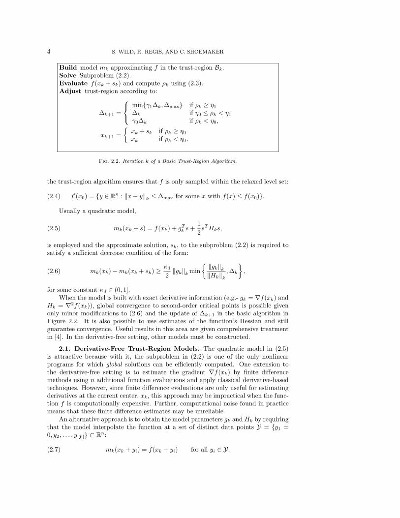
Build model mk approximating f in the trust-region Bk.Solve Subproblem (2.2).Evaluate f(xk + sk) and compute ρk using (2.3).Adjust trust-region according to:

∆k+1 =

minγ1∆k,∆max if ρk ≥ η1

∆k if η0 ≤ ρk < η1

γ0∆k if ρk < η0,

xk+1 =

xk + sk if ρk ≥ η0

xk if ρk < η0.

Fig. 2.2. Iteration k of a Basic Trust-Region Algorithm.

the trust-region algorithm ensures that f is only sampled within the relaxed level set:

L(x0) = y ∈ Rn : ‖x− y‖k ≤ ∆max for some x with f(x) ≤ f(x0).(2.4)

Usually a quadratic model,

mk(xk + s) = f(xk) + gTk s +

1

2sT Hks,(2.5)

is employed and the approximate solution, sk, to the subproblem (2.2) is required tosatisfy a sufficient decrease condition of the form:

mk(xk)−mk(xk + sk) ≥ κd

2‖gk‖k min

‖gk‖k‖Hk‖k

,∆k

,(2.6)

for some constant κd ∈ (0, 1].When the model is built with exact derivative information (e.g.- gk = ∇f(xk) and

Hk = ∇2f(xk)), global convergence to second-order critical points is possible givenonly minor modifications to (2.6) and the update of ∆k+1 in the basic algorithm inFigure 2.2. It is also possible to use estimates of the function’s Hessian and stillguarantee convergence. Useful results in this area are given comprehensive treatmentin [4]. In the derivative-free setting, other models must be constructed.

2.1. Derivative-Free Trust-Region Models. The quadratic model in (2.5)is attractive because with it, the subproblem in (2.2) is one of the only nonlinearprograms for which global solutions can be efficiently computed. One extension tothe derivative-free setting is to estimate the gradient ∇f(xk) by finite differencemethods using n additional function evaluations and apply classical derivative-basedtechniques. However, since finite difference evaluations are only useful for estimatingderivatives at the current center, xk, this approach may be impractical when the func-tion f is computationally expensive. Further, computational noise found in practicemeans that these finite difference estimates may be unreliable.

An alternative approach is to obtain the model parameters gk and Hk by requiringthat the model interpolate the function at a set of distinct data points Y = y1 =0, y2, . . . , y|Y| ⊂ R

n:

mk(xk + yi) = f(xk + yi) for all yi ∈ Y.(2.7)

ORBIT 5

n 10 20 30 40 50 60 70 80 90 100(n+1)(n+2)

2 66 231 496 861 1326 1891 2556 3321 4186 5151Table 2.1

Number of Interpolation Points Needed to Uniquely Define a Full Quadratic Model.

The idea of forming quadratic models by interpolation for optimization without deriva-tives was proposed by Winfield in the late 1960’s [30] and revived in the mid 1990’sindependently by Powell (UOBYQA [23]) and Conn, Scheinberg, and Toint (DFO [5]).

These methods rely heavily on results from multivariate interpolation, a problemmuch more difficult than its univariate counterpart [28]. In particular, since the di-mension of quadratics in R

n is p = 12 (n+1)(n+2), at least p function evaluations must

be done to provide enough interpolation points to ensure uniqueness of the quadraticmodel. Further, these points must satisfy strict geometric conditions for the interpo-lation problem in (2.7) to be well-posed. These geometric conditions have receivedrecent treatment in [7], where Taylor-like error bounds between the polynomial mod-els and the true function were proposed. A quadratic model interpolating 6 points inR

2 is shown in the lower left corner of Figure 2.1.A significant drawback of these full quadratic methods is that the number of

interpolation points they strive for is quadratic in the dimension of the problem. Forexample, we see in Table 2.1 that when n = 30, nearly 500 function evaluationsare required before the first fully quadratic surrogate model can be constructed andthe subproblem optimization can begin. Of course, fully linear models can also beobtained in n + 1 function evaluations.

Before proceeding, we note that Powell has addressed this difficulty by proposingto satisfy (2.7) uniquely by certain underdetermined quadratics [24]. He developedNEWUOA, a complex but computationally efficient Fortran code using updates of themodel such that the change in the model’s Hessian is of minimum Frobenius norm[25]. A similar approach is used in a later version of the DFO package [6].

2.2. Fully Linear Models. In order to avoid geometric conditions on O(n2)points, we will rely on a class of so-called fully linear interpolation models, which canbe formed using as few as n + 1 function evaluations. To establish Taylor-like errorbounds, the function f must be reasonably smooth. Throughout the sequel we willmake the following assumptions on the function f :(Assumption on Function) f ∈ C1[Ω] for some open Ω ⊃ L(x0), ∇f is Lipschitz

continuous on L(x0), and f is bounded on L(x0).We borrow the following definition from [7] and note that three similar conditionsdefine fully quadratic models.

Definition 2.1. For fixed κf > 0, κg > 0, xk such that f(xk) ≤ f(x0), and∆ ∈ (0,∆max] defining B = x ∈ R

n : ‖x− xk‖k ≤ ∆, a model m ∈ C1[Ω] is said tobe fully linear on B if for all x ∈ B:

|f(x)−m(x)| ≤ κf∆2,(2.8)

‖∇f(x)−∇m(x)‖ ≤ κg∆.(2.9)

If a fully linear model can be obtained for any ∆ ∈ (0,∆max], these conditionsensure that an approximation to even the true function’s gradient can achieve anydesired degree of precision within a small enough neighborhood of xk. As exemplifiedin [7], fully linear interpolation models are defined by geometry conditions on theinterpolation set. In Section 4 we will explore the conditions (2.8) and (2.9) for theradial basis function models introduced next.


3. Radial Basis Functions. Quadratic surrogates of the form (2.5) have thebenefit of being easy to implement while still being able to model curvature of theunderlying function f . Another way to model curvature is to consider interpolatingsurrogates, which are linear combinations of nonlinear basis functions and satisfy (2.7)

for the interpolation points yj|Y|j=1. One possible model is of the form:

mk(xk + s) =

|Y|∑

j=1

λjφ(‖s− yj‖) + p(s),(3.1)

where φ : R+ → R is a univariate function and p ∈ Pnd−1, where Pn

d−1 is the (trivialif d = 0) space of polynomials in n variables of total degree no more than d − 1. Inaddition to guaranteeing uniqueness of the model mk, the polynomial tail p ensuresthat mk belongs to a linear space that also contains the polynomial space Pn

d−1.Such models are called radial basis functions (RBFs) because mk(xk + s)− p(s)

is a linear combination of shifts of the function φ(‖x‖), which is constant on spheres

in Rn. For concreteness, we represent the polynomial tail by p(s) =

∑pi=1 νiπi(s),

for p =dimPnd−1 and π1(s), . . . , πp(s), a basis for Pn

d−1. Some examples of popularradial functions are given in Table 3.1.

For fixed coefficients λ, these radial functions are all twice continuously differen-tiable. We briefly note that for an RBF model to be twice continuously differentiable,the radial function φ must be both twice continuously differentiable and have a deriva-tive that vanishes at the origin. We then have relatively simple analytic expressionsfor both the gradient,

∇mk(xk + s) =

|Y|∑

i=1

λiφ′(‖s− yi‖)

s− yi

‖s− yi‖+∇p(s),(3.2)

and Hessian, provided in (4.15), of the model.In addition to being sufficiently smooth, these radial functions in Table 3.1 all

share the property of conditional positive definiteness [28].Definition 3.1. Let π be a basis for Pn

d−1, with the convention that π = ∅ ifd = 0. A function φ is said to be Conditionally Positive Definite (CPD) of order d

if for all sets of distinct points Y ⊂ Rn and all λ 6= 0 satisfying

∑|Y|j=1 λjπ(yj) = 0,

the quadratic form∑|Y|

i,j=1 λjφ(‖yi − yj‖)λj is positive.This property ensures that there exists a unique model of the form (3.1) provided

that p points in Y are poised for interpolation in Pnd−1. A set of p points is said to

be poised for interpolation in Pnd−1 if the zero polynomial is the only polynomial in

Pnd−1 which vanishes at all p points. Conditional positive definiteness of a function is

usually proved by Fourier transforms [3, 28] and is beyond the scope of the presentwork. Before addressing solution techniques, we note that if φ is CPD of order d, thenit is also CPD of order d ≥ d.

3.1. Obtaining Model Parameters. We now illustrate one method for ob-taining the parameters defining an RBF model that interpolates data as in (2.7) atknots in Y. Defining the matrices Π ∈ R

p×|Y| and Φ ∈ R|Y|×|Y|, as Πi,j = πi(yj) and

Φi,j = φ(‖yi − yj‖), respectively, we consider the symmetric linear system:

[

Φ ΠT

Π 0

] [

λ

ν

]

=

[

f

0

]

.(3.3)

ORBIT 7

Since πj(s)pj=1 forms a basis for Pnd−1, the interpolation set Y being poised for

interpolation in Pnd is equivalent to rank(Π)=dimPn

d−1 = p. It is then easy to see thatfor CPD functions of order d, a sufficient condition for the nonsingularity of (3.3) isthat the points in Y are distinct and yield a ΠT of full column rank. It is instructiveto note that, as in polynomial interpolation, these are geometric conditions on theinterpolation nodes and are independent of the data values in f .

We will exploit this property of RBFs by using a null-space method (see forexample [1]) for solving the symmetric system in (3.3). Suppose that ΠT is of fullcolumn rank and admits the truncated QR factorization ΠT = QR and hence R ∈R

(n+1)×(n+1) is nonsingular. By the lower set of equations in (3.3) we must haveλ = Zω for ω ∈ R

|Y|−n−1 and any orthogonal basis Z for N (Π) (e.g.- from theorthogonal columns of a full QR decomposition) . Hence (3.3) reduces to:

ZT ΦZω = ZT f(3.4)

Rν = QT (f − ΦZω).(3.5)

By the rank condition on ΠT and the distinctness of the points in Y, ZT ΦZ is positivedefinite for any φ that is CPD of at most order d. Hence the matrix that determinesthe RBF coefficients λ admits the Cholesky factorization:

ZT ΦZ = LLT(3.6)

for a nonsingular lower triangular L. Since Z is orthogonal we immediately note thebound:

‖λ‖ =∥

∥ZL−T L−1ZT f∥

∥ ≤∥

∥L−1∥

∥

2 ‖f‖ ,(3.7)

which will prove useful for the analysis in Section 4.2.

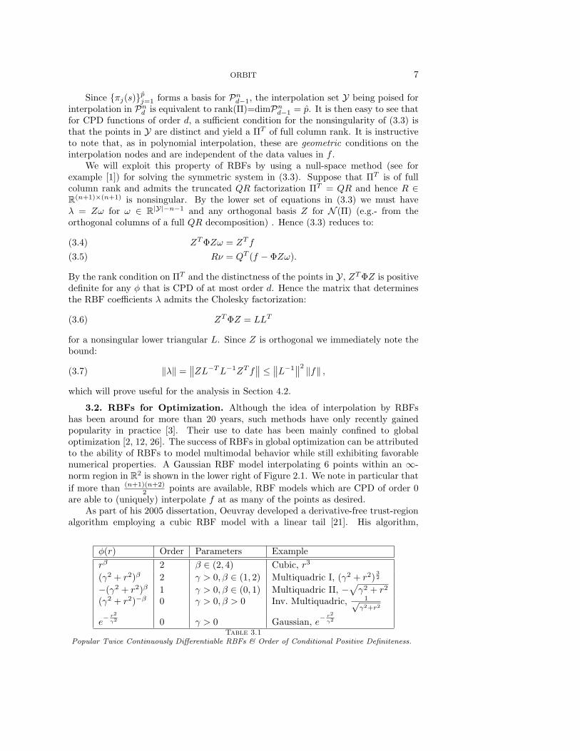
3.2. RBFs for Optimization. Although the idea of interpolation by RBFshas been around for more than 20 years, such methods have only recently gainedpopularity in practice [3]. Their use to date has been mainly confined to globaloptimization [2, 12, 26]. The success of RBFs in global optimization can be attributedto the ability of RBFs to model multimodal behavior while still exhibiting favorablenumerical properties. A Gaussian RBF model interpolating 6 points within an ∞-norm region in R

2 is shown in the lower right of Figure 2.1. We note in particular that

if more than (n+1)(n+2)2 points are available, RBF models which are CPD of order 0

are able to (uniquely) interpolate f at as many of the points as desired.As part of his 2005 dissertation, Oeuvray developed a derivative-free trust-region

algorithm employing a cubic RBF model with a linear tail [21]. His algorithm,

φ(r) Order Parameters Example

rβ 2 β ∈ (2, 4) Cubic, r3

(γ2 + r2)β 2 γ > 0, β ∈ (1, 2) Multiquadric I, (γ2 + r2)3

2

−(γ2 + r2)β 1 γ > 0, β ∈ (0, 1) Multiquadric II, −√

γ2 + r2

(γ2 + r2)−β 0 γ > 0, β > 0 Inv. Multiquadric, 1√γ2+r2

e− r2

γ2 0 γ > 0 Gaussian, e− r2

γ2

Table 3.1

Popular Twice Continuously Differentiable RBFs & Order of Conditional Positive Definiteness.


BOOSTERS, was motivated by problems in the area of medical image registrationand was subsequently modified to include gradient information when available [22].Convergence theory was based on the literature available at the time [4].

Step 1: Find n + 1 affinely independent points:AffPoints(Dk, θ0, θ1,∆k) (detailed in Figure 4.2)

Step 2: Add up to pmax − n− 1 additional points to Y:AddPoints(Dk,θ2,pmax)

Step 3: Obtain RBF model parameters from (3.4) and (3.5).Step 4: While ‖∇mk(xk)‖ ≤ ǫg

2 :If mk is fully linear in Bg

k = x ∈ Rn : ‖xk − x‖k ≤ (2κg)

−1ǫg,Return.

Else,Obtain a model mk that is fully linear in Bg

k,Set ∆k =

ǫg

2κg.

Step 5: Approximately solve subproblem (2.2) to obtain a step sk satisfying (4.18),Evaluate f(xk + sk).

Step 6: Update trust-region parameters:

∆k+1 =

minγ1∆k,∆max if ρk ≥ η1

∆k if ρk < η1 and mk is not fully linear on Bk

γ0∆k if ρk < η1 and mk is fully linear on Bk

xk+1 =

xk + sk if ρk ≥ η1

xk + sk if ρk > η0 and mk is fully linear on Bk

xk else

Step 7: Evaluate a model-improving point if ρk ≤ η0 and mk is not fully linear onBk.

Fig. 4.1. Iteration k of the ORBIT Algorithm.

4. The ORBIT Algorithm. In this section we detail our algorithm, ORBIT, andestablish several of the computational techniques employed. Given trust-region inputs0 ≤ η0 ≤ η1 < 1, 0 < γ0 < 1 < γ1, 0 < ∆0 ≤ ∆max, and x0 ∈ R

n, and additionalinputs 0 < θ1 ≤ θ−1

0 ≤ 1, θ2 > 0, κf , κg, ǫg > 0, and pmax > n + 1, an outline of thekth iteration of the algorithm is provided in Figure 4.1.

Besides the current trust-region center and radius, the algorithm works with aset of displacements, Dk, from the current center xk. This set consists of all pointsat which the true function value is known:

di ∈ Dk ⇐⇒ f(xk + di) is known.(4.1)

Since evaluation of f is computationally expensive, we stress the importance of havingcomplete knowledge of all points previously evaluated by the algorithm. This is afundamental difference between ORBIT and previous algorithms in [22, 23, 25], where,in order to reduce linear algebraic costs, the interpolation set was allowed to change byat most one point. For these algorithms, once a point is dropped from the interpolationset it may never return. In our view, these evaluated points contain information whichcould allow the model to gain additional insight into the function which is especially

ORBIT 9

valuable when only a limited number of evaluations is possible. This is particularlywhen larger trust-regions, especially seen in the early phases of the optimization,result in large steps.

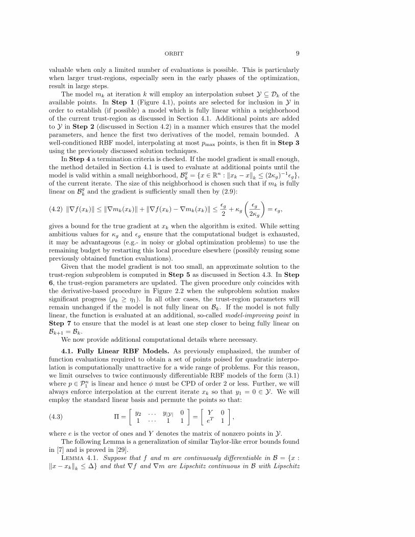
The model mk at iteration k will employ an interpolation subset Y ⊆ Dk of theavailable points. In Step 1 (Figure 4.1), points are selected for inclusion in Y inorder to establish (if possible) a model which is fully linear within a neighborhoodof the current trust-region as discussed in Section 4.1. Additional points are addedto Y in Step 2 (discussed in Section 4.2) in a manner which ensures that the modelparameters, and hence the first two derivatives of the model, remain bounded. Awell-conditioned RBF model, interpolating at most pmax points, is then fit in Step 3using the previously discussed solution techniques.

In Step 4 a termination criteria is checked. If the model gradient is small enough,the method detailed in Section 4.1 is used to evaluate at additional points until themodel is valid within a small neighborhood, Bg

k = x ∈ Rn : ‖xk − x‖k ≤ (2κg)

−1ǫg,of the current iterate. The size of this neighborhood is chosen such that if mk is fullylinear on Bg

k and the gradient is sufficiently small then by (2.9):

‖∇f(xk)‖ ≤ ‖∇mk(xk)‖+ ‖∇f(xk)−∇mk(xk)‖ ≤ ǫg

2+ κg

(

ǫg

2κg

)

= ǫg,(4.2)

gives a bound for the true gradient at xk when the algorithm is exited. While settingambitious values for κg and ǫg ensure that the computational budget is exhausted,it may be advantageous (e.g.- in noisy or global optimization problems) to use theremaining budget by restarting this local procedure elsewhere (possibly reusing somepreviously obtained function evaluations).

Given that the model gradient is not too small, an approximate solution to thetrust-region subproblem is computed in Step 5 as discussed in Section 4.3. In Step6, the trust-region parameters are updated. The given procedure only coincides withthe derivative-based procedure in Figure 2.2 when the subproblem solution makessignificant progress (ρk ≥ η1). In all other cases, the trust-region parameters willremain unchanged if the model is not fully linear on Bk. If the model is not fullylinear, the function is evaluated at an additional, so-called model-improving point inStep 7 to ensure that the model is at least one step closer to being fully linear onBk+1 = Bk.

We now provide additional computational details where necessary.

4.1. Fully Linear RBF Models. As previously emphasized, the number offunction evaluations required to obtain a set of points poised for quadratic interpo-lation is computationally unattractive for a wide range of problems. For this reason,we limit ourselves to twice continuously differentiable RBF models of the form (3.1)where p ∈ Pn

1 is linear and hence φ must be CPD of order 2 or less. Further, we willalways enforce interpolation at the current iterate xk so that y1 = 0 ∈ Y. We willemploy the standard linear basis and permute the points so that:

Π =

[

y2 . . . y|Y| 01 · · · 1 1

]

=

[

Y 0eT 1

]

,(4.3)

where e is the vector of ones and Y denotes the matrix of nonzero points in Y.The following Lemma is a generalization of similar Taylor-like error bounds found

in [7] and is proved in [29].Lemma 4.1. Suppose that f and m are continuously differentiable in B = x :

‖x− xk‖k ≤ ∆ and that ∇f and ∇m are Lipschitz continuous in B with Lipschitz


constants γf and γm, respectively. Further suppose that m satisfies the interpolationconditions in (2.7) at a set of points Y = y1 = 0, y2, . . . , yn+1 ⊆ B − xk such that∥

∥Y −1∥

∥ ≤ ΛY

ck∆ , where ck (introduced in Section 2) is only related to the trust-regionnorm. Then for any x ∈ B:

• |m(x)− f(x)| ≤ √nc2k (γf + γm)

(

52ΛY + 1

2

)

∆2, and• ‖∇m(x)−∇f(x)‖ ≤ 5

2

√nΛY ck (γf + γm) ∆.

We note that Lemma 4.1 applies to many models in addition to the RBFs consid-ered here. In particular, it says that if a model with a Lipschitz continuous gradientinterpolates a function on a sufficiently affinely independent set of points, there existconstants κf , κg > 0 independent of ∆ such that conditions (2.8) and (2.9) are sat-isfied and hence m is fully linear on B. The assumption that the model’s gradient isLipschitz continuous is milder than assuming that the model is twice differentiable.However, in practice, we expect that this assumption would in fact be guaranteed byenforcing a bound on the norm of the model’s Hessian.

It remains to show that n + 1 points in B − xk can be efficiently obtained suchthat the norm of Y −1 can be bounded by a quantity of the form ΛY

ck∆ . In ORBIT, weensure this by working with a QR factorization of the normalized points as justifiedin the following lemma.

Lemma 4.2. If all QR pivots of 1ck∆Y satisfy |rii| ≥ θ1 > 0, then

∥

∥Y −1∥

∥ ≤n

n−1

2 θ−n1

ck∆ .

Proof. If y2, . . . , yn+1 ⊆ B−xk, all columns of the normalized matrix Y = 1ck∆Y

satisfy∥

∥

∥Yj

∥

∥

∥≤ 1. Letting QR = Y denote a QR factorization of the matrix Y , and

0 ≤ σn ≤ · · · ≤ σ1 ≤√

n denote the ordered singular values of Y , we have

σnσn−11 ≥

n∏

i=1

σi = |det(Y )| = |det(R)| =n

∏

i=1

|rii|.(4.4)

If each of the QR pivots satisfy |rii| ≥ θ1 > 0, we have the admittedly crude bound:

∥

∥Y −1∥

∥ =1

ck∆

∥

∥

∥Y −1

∥

∥

∥=

1

ck∆

1

σn

≤ 1

ck∆

nn−1

2

θn1

.(4.5)

While other bounds based on the size of the QR pivots are possible, we note thatthe one above does not rely on pivoting strategies beyond the θ1 thresholding. Furtherpivoting may limit the number of recently sampled points that can be included in theinterpolation set, particularly since choosing points in B that are farther away fromthe current iterate may prevent subsequent pivots from being sufficiently large.

We note that if ∆ in Lemmas 4.1 and 4.2 is chosen to be the current trust-regionradius ∆k, the design of the algorithm may mean that there are very few points withinB at which f has been evaluated. For this reason, we will look to make mk fully linearwithin an enlarged region defined by x : ‖x− xk‖k ≤ θ0∆k for a constant θ0 ≥ 1.We note that this constant still ensures that the model is fully linear within the trust-region Bk, provided that the constants κf and κg are suitably altered in Lemma 4.1.

The subroutine AffPoints given in Figure 4.2 details our method of constructinga model which is fully linear on Bk. We note that the projections in 2. and 3b. areexactly the magnitude of the pivot that results from adding point dj to Y.

Because of the form of Y , it is straightforward to see that for any θ1 ∈ (0, θ−10 ],

an interpolation set Y ⊆ B − xk can be constructed such that all QR pivots satisfy

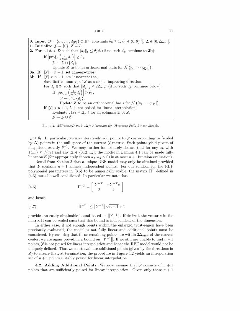
ORBIT 11

0. Input D = d1, . . . , d|D| ⊂ Rn, constants θ0 ≥ 1, θ1 ∈ (0, θ−1

0 ], ∆ ∈ (0,∆max].1. Initialize Y = 0, Z = In.2. For all dj ∈ D such that ‖dj‖k ≤ θ0∆ (if no such dj , continue to 3b):

If∣

∣

∣projZ

(

1θ0∆

dj

)∣

∣

∣≥ θ1,

Y ← Y ∪ dj,Update Z to be an orthonormal basis for N

(

[y1 · · · y|Y|])

.3a. If |Y| = n + 1, set linear=true.3b. If |Y| < n + 1, set linear=false,

Save first column z1 of Z as a model-improving direction,For dj ∈ D such that ‖dj‖k ≤ 2∆max (if no such dj , continue below):

If∣

∣

∣projZ

(

1θ0∆

dj

)∣

∣

∣≥ θ1,

Y ← Y ∪ dj,Update Z to be an orthonormal basis for N

(

[y1 · · · y|Y|])

.If |Y| < n + 1, Y is not poised for linear interpolation,

Evaluate f(xk + ∆zi) for all columns zi of Z,Y ← Y ∪ Z.

Fig. 4.2. AffPoints(D, θ0, θ1, ∆): Algorithm for Obtaining Fully Linear Models.

rii ≥ θ1. In particular, we may iteratively add points to Y corresponding to (scaledby ∆) points in the null space of the current Y matrix. Such points yield pivots ofmagnitude exactly θ−1

0 . We may further immediately deduce that for any xk withf(xk) ≤ f(x0) and any ∆ ∈ (0,∆max], the model in Lemma 4.1 can be made fullylinear on B (for appropriately chosen κf , κg > 0) in at most n+1 function evaluations.

Recall from Section 3 that a unique RBF model may only be obtained providedthat Y contains n + 1 affinely independent points. For our solution for the RBFpolynomial parameters in (3.5) to be numerically stable, the matrix ΠT defined in(4.3) must be well-conditioned. In particular we note that

Π−T =

[

Y −T −Y −T e

0 1

]

(4.6)

and hence

∥

∥Π−T∥

∥ ≤∥

∥Y −1∥

∥

√n + 1 + 1(4.7)

provides an easily obtainable bound based on∥

∥Y −1∥

∥. If desired, the vector e in thematrix Π can be scaled such that this bound is independent of the dimension.

In either case, if not enough points within the enlarged trust-region have beenpreviously evaluated, the model is not fully linear and additional points must beconsidered. By ensuring that these remaining points are within 2∆max of the currentcenter, we are again providing a bound on

∥

∥Y −1∥

∥. If we still are unable to find n + 1points, Y is not poised for linear interpolation and hence the RBF model would not beuniquely defined. Thus we must evaluate additional points (given by the directions inZ) to ensure that, at termination, the procedure in Figure 4.2 yields an interpolationset of n + 1 points suitably poised for linear interpolation.

4.2. Adding Additional Points. We now assume that Y consists of n + 1points that are sufficiently poised for linear interpolation. Given only these n + 1


points, λ = 0 is the unique solution to (3.3) and hence the RBF model in (3.1) islinear. In order to take advantage of the nonlinear modeling benefits of RBFs it isthus clear that additional points should be added to Y. Note that by Lemma 4.1,adding these points will not affect the property of a model being fully linear.

We now detail ORBIT’s method of adding additional model points to Y whilemaintaining bounds on the conditioning of the system (3.4). In [21] the RBF inter-polation set generally changes by at most one point from one iteration to the nextand is based on an updating technique applied to the larger system in (3.3). ORBIT’smethod largely follows the development in [2] and directly addresses the conditioningof the system used by our solution techniques.

Employing the notation of Section 3.1, we now consider what happens when y ∈R

n is added to the interpolation set Y. We denote the basis function and polynomialmatrices obtained when this new point is added as Φy and ΠT

y , respectively:

Φy =

[

Φ φy

φTy φ(0)

]

, ΠTy =

[

ΠT

π(y)

]

.(4.8)

As suggested by Lemmas 4.1 and 4.2, we note that in practice we work with a scaledpolynomial matrix ΠT

y . For example, for our linear polynomial matrix, we scale the

displacements in Y by ∆k, eg.- π(

y∆k

)

. This scaling does not affect the analysis of

the algorithm using linear tails in [29].We begin by noting that by applying n + 1 Givens rotations to the full QR

factorization of ΠT , we obtain an orthogonal basis for N (Πy) of the form:

Zy =

[

Z Qg

0 g

]

,(4.9)

where, as in Section 3.1, Z is any orthogonal basis for N (Π). Hence, ZTy ΦZy is of the

form:

ZTy ΦZy =

[

ZT ΦZ v

vT σ

]

,(4.10)

and it can easily be shown that:

LTy =

[

LT L−1v

0

√

σ − ‖L−1v‖2

]

, L−Ty =

L−T −L−T L−1v√σ−‖L−1v‖2

0 1√σ−‖L−1v‖2

(4.11)

yields LyLTy = ZT

y ΦZy. Careful algebra shows that:

v = ZT (ΦQg + φy g)(4.12)

σ = gT QT ΦQg + 2gT QT φy g + φ(0)g2.(4.13)

Assuming that both Y and the new point y belong to x ∈ Rn : ‖x‖k ≤ 2∆max,

the quantities ‖x− z‖ : x, y ∈ Y ∪y are all of magnitude no more than 4ck∆max.Using the isometry of Zy and (Qg, g) we hence have the bound:

‖v‖ ≤√

|Y|(|Y|+ 1) max|φ(r)| : r ∈ [0, 4ck∆max].(4.14)

Provided that L−1 was previously well-conditioned, the resulting factors L−1y

remain bounded provided that

√

σ − ‖L−1v‖2 is bounded away from 0. Hence our

ORBIT 13

Initialize s = − ∇mk(xk)‖∇mk(xk)‖k

∆k.

While mk(xk)−mk(xk + s) < κd

2 ‖∇mk(xk)‖min

‖∇mk(xk)‖κH

,‖∇mk(xk)‖‖∇mk(xk)‖k

∆k

:s← sα.

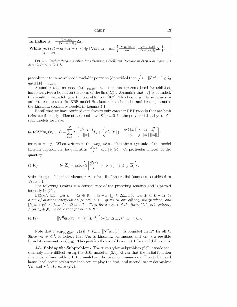
Fig. 4.3. Backtracking Algorithm for Obtaining a Sufficient Decrease in Step 5 of Figure 4.1(α ∈ (0, 1), κd ∈ (0, 1]).

procedure is to iteratively add available points to Y provided that

√

σ − ‖L−1v‖2 ≥ θ2

until |Y| = pmax.Assuming that no more than pmax − n − 1 points are considered for addition,

induction gives a bound on the norm of the final L−1Y . Assuming that ‖f‖ is bounded,

this would immediately give the bound for λ in (3.7). This bound will be necessary inorder to ensure that the RBF model Hessians remain bounded and hence guaranteethe Lipschitz continuity needed in Lemma 4.1.

Recall that we have confined ourselves to only consider RBF models that are bothtwice continuously differentiable and have ∇2p ≡ 0 for the polynomial tail p(·). Forsuch models we have:

∇2mk(xk + s) =

|Y|∑

i=1

λi

[

φ′(‖zi‖)‖zi‖

In +

(

φ′′(‖zi‖)−φ′(‖zi‖)‖zi‖

)

zi

‖zi‖zTi

‖zi‖

]

,(4.15)

for zi = s − yi. When written in this way, we see that the magnitude of the model

Hessian depends on the quantities∣

∣

∣

φ′(r)r

∣

∣

∣and |φ′′(r)|. Of particular interest is the

quantity:

b2(∆) = max

2

∣

∣

∣

∣

φ′(r)

r

∣

∣

∣

∣

+ |φ′′(r)| : r ∈ [0,∆]

,(4.16)

which is again bounded whenever ∆ is for all of the radial functions considered inTable 3.1.

The following Lemma is a consequence of the preceding remarks and is provedformally in [29].

Lemma 4.3. Let B = x ∈ Rn : ‖x− xk‖k ≤ 2∆max. Let Y ⊂ B − xk be

a set of distinct interpolation points, n + 1 of which are affinely independent, and|f(xk + yi)| ≤ fmax for all yi ∈ Y. Then for a model of the form (3.1) interpolatingf on xk + Y, we have that for all x ∈ B:

∥

∥∇2mk(x)∥

∥ ≤ |Y|∥

∥L−1∥

∥

2b2(4ck∆max)fmax =: κH .(4.17)

Note that if supx∈L(x0) |f(x)| ≤ fmax,∥

∥∇2mk(x)∥

∥ is bounded on Rn for all k.

Since mk ∈ C2, it follows that ∇m is Lipschitz continuous and κH is a possibleLipschitz constant on L(x0). This justifies the use of Lemma 4.1 for our RBF models.

4.3. Solving the Subproblem. The trust-region subproblem (2.2) is made con-siderably more difficult using the RBF model in (3.1). Given that the radial functionφ is chosen from Table 3.1, the model will be twice continuously differentiable, andhence local optimization methods can employ the first- and second- order derivatives∇m and ∇2m to solve (2.2).


10 20 30 40 50 60 70 80 90 100

101

102

103

Number of Function Evaluations

Mean Best Function Value

ORBIT (2)ORBIT (∞)Newuoa (n+2)Newuoa (2n+1)NMSMAXAPPS

20 40 60 80 100 120 140 160

101

102

103




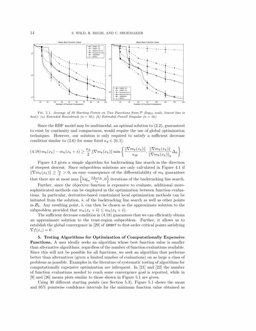
Fig. 5.1. Average of 30 Starting Points on Two Functions from P (log10 scale, lowest line isbest): (a) Extended Rosenbrock (n = 10); (b) Extended Powell Singular (n = 16).

Since the RBF model may be multimodal, an optimal solution to (2.2), guaranteedto exist by continuity and compactness, would require the use of global optimizationtechniques. However, our solution is only required to satisfy a sufficient decreasecondition similar to (2.6) for some fixed κd ∈ (0, 1]:

mk(xk)−mk(xk + s) ≥ κd

2‖∇mk(xk)‖min

‖∇mk(xk)‖κH

,‖∇mk(xk)‖‖∇mk(xk)‖k

∆k

.(4.18)

Figure 4.3 gives a simple algorithm for backtracking line search in the directionof steepest descent. Since subproblem solutions are only calculated in Figure 4.1 if‖∇mk(xk)‖ ≥ ǫg

2 > 0, an easy consequence of the differentiability of mk guarantees

that there are at most max

logα2∆kκH

ǫg, 0

iterations of the backtracking line search.

Further, since the objective function is expensive to evaluate, additional more-sophisticated methods can be employed in the optimization between function evalua-tions. In particular, derivative-based constrained local optimization methods can beinitiated from the solution, s, of the backtracking line search as well as other pointsin Bk. Any resulting point, s, can then be chosen as the approximate solution to thesubproblem provided that mk(xk + s) ≤ mk(xk + s).

The sufficient decrease condition in (4.18) guarantees that we can efficiently obtainan approximate solution to the trust-region subproblem. Further, it allows us toestablish the global convergence in [29] of ORBIT to first-order critical points satisfying∇f(x∗) = 0 .

5. Testing Algorithms for Optimization of Computationally ExpensiveFunctions. A user ideally seeks an algorithm whose best function value is smallerthan alternative algorithms, regardless of the number of function evaluations available.Since this will not be possible for all functions, we seek an algorithm that performsbetter than alternatives (given a limited number of evaluations) on as large a class ofproblems as possible. Examples in the literature of systematic testing of algorithms forcomputationally expensive optimization are infrequent. In [21] and [22] the numberof function evaluations needed to reach some convergence goal is reported, while in[9] and [26] means plots similar to those shown in Figure 5.1 are given.

Using 30 different starting points (see Section 5.3), Figure 5.1 shows the meanand 95% pointwise confidence intervals for the minimum function value obtained as

ORBIT 15

a function of the number of evaluations performed. Such plots are useful for deter-mining the number of evaluations needed to obtain some desired function value andfor providing insight into an algorithm’s average progress. However, by grouping allstarting points together, we are unable to determine the relative success of algorithmsusing the same starting point. We now discuss one way to complement the meansplots in Figure 5.1.

5.1. Performance and Data Profiles. In [8], Dolan and More develop a pro-cedure for visualizing the relative success of solvers on a set of benchmark problems.Their performance profiles are gaining currency in the optimization community andare defined by three characteristics: a set of benchmark problems P, a convergencetest T , and a set of algorithms/solvers S. Based on the convergence test, a perfor-mance metric tp,s to be minimized (e.g.- the amount of computing time required tomeet some termination criteria) is obtained for each (p, s) ∈ P × S. For a pair (p, s),the performance ratio

rp,s =tp,s

mintp,s : s ∈ S(5.1)

defines the success of an algorithm relative to the other algorithms in S. The bestalgorithm for a particular problem attains the lower bound rp,s = 1, while rp,s = ∞if an algorithm fails to meet the convergence test. For algorithm s, the fraction ofproblems where the performance ratio is at most α is:

ρs(α) =1

|P| size

p ∈ P : rp,s ≤ α

.(5.2)

The performance profile ρs(α) is a probability distribution function capturing theprobability that the performance ratio for s is within a factor α of the best possi-ble ratio. Conclusions based on ρs(α) should only be extended to other problems,convergence tests, and algorithms similar to those in P, T , and S.

Extensions to the computationally expensive and derivative-free settings haverecently been examined in [19]. The convergence test used there is

f(x0)− f(x) ≥ (1− τ)(f(x0)− fL),(5.3)

which is equivalent to requiring that x achieve a reduction which is at least 1−τ of thebest possible reduction f(x0) − fL. The parameter fL is chosen to be the minimumfunction value found by any of the solvers in S within the maximum number offunction evaluations, µf . This convergence test allows a user to choose an accuracylevel τ appropriate for the resolution of their simulator and goals of their application.

We assume that any computations done by an algorithm except evaluation of thefunction are negligible and that the time required to evaluate a function is the sameat any point of interest. The performance metric tp,s used here is then the number offunction evaluations needed to satisfy the convergence test (5.3) for a given τ > 0.

Since performance profiles do not show the number of function evaluations neededto solve a problem, data profiles are also introduced in [19]. The data profile,

ds(κ) =1

|P| size

p ∈ P :tp,s

np + 1≤ κ

,(5.4)

where np is the dimension of problem p ∈ P, represents the percentage of problemsthat can be solved by solver s with the equivalent of κ (simplex) gradient estimates,corresponding to κ(n + 1) function evaluations. A data profile is again paired withan accuracy level τ > 0 associated with the convergence test (5.3).


5.2. Algorithms Tested. We compared ORBIT to a number of competitive se-rial algorithms for derivative-free optimization. Here we report the results of thistesting for three freely available algorithms, APPSPACK, NMSMAX, and NEWUOA. Noimplementation of the BOOSTERS code in [21, 22] is available.

All algorithms considered required an initial starting point, x0, a maximum num-ber of function evaluations, µf , and a starting parameter, ∆0. The values of theseinputs change from problem to problem but are kept consistent across all of the algo-rithms considered. We note that appropriate scaling of variables is a key determinantof performance of derivative-free algorithms and any knowledge of the specific ap-plication by the user should be provided to these algorithms in order to obtain ascaled trust-region norm or pattern. For our tests, we assumed no such knowledgewas available and gave all algorithms standard (unit) scaling in each variable.

We used the APPSPACK (version 4.0.2) pattern search method because APPSPACK

performed well in recent testing on a groundwater problem [9]. APPSPACK is an asyn-chronous parallel pattern search method [11, 15], which systematically samples thefunction along search directions defining a pattern (which is by default the set ofplus and minus coordinate directions ±e1, . . . ,±en), scaled much the same way asa trust-region. APPSPACK can be run in serial mode (used here) and can handle con-straints. We note that since APPSPACK is designed to be run in parallel, its full poweris not demonstrated in serial mode. This code requires a choice of scaling, an initialstep size, and a final pattern size. We set the scaling to 1, the initial step size to ∆0

to conform with the other algorithms tested, and the final pattern size to 10−19∆0 toensure that the algorithm will not terminate until it reaches the maximum number offunction evaluations.

An implementation of the Nelder-Mead method was used because this methodis popular among application scientists. Many implementations of this method existand we used the NMSMAX code, available from the Matrix Computation Toolbox [13],because it came with default inputs which performed well. The NMSMAX code requiresa choice of starting simplex and final step size. We used a right-angled simplex withside length ∆0 to conform with the other algorithms tested and a final step size of 0to ensure that the algorithm will not terminate until it reaches the maximum numberof function evaluations.

We used the NEWUOA code because it performed best among quadratic model-based methods in comparisons in [21, 22]. Powell’s Fortran NEWUOA code [25] requiresan initial radius which we set to ∆0, a final radius which we set to 10−15∆0 to againensure that the algorithm will not terminate until it reaches the maximum number offunction evaluations, and a number of interpolation points p. We tested two variants,one with Powell’s recommended p = 2n + 1 and one with the minimum p = n + 2, astrategy which may work well in the initial stages of the optimization.

We implement ORBIT using a cubic RBF model with both 2-norm and ∞-normtrust-regions. For all experiments we used the ORBIT (Figure 4.1) parameters: η0 = 0,η1 = .2, γ0 = 1

2 , γ1 = 2, ∆max = 103∆0, θ0 = 10 θ1 = 10−3, θ2 = 10−7, ǫg = 10−10,and pmax = 3n. For the backtracking line search algorithm in Figure 4.3, we setκd = 10−4 and α = .9. In the ORBIT implementation tested here, we also relied onthe FMINCON routine from MATLAB [17] which is based on a sequential quadraticprogramming (SQP) method.

On the largest problem tested here (n = 18), ORBIT required nearly .5 seconds peraverage iteration on a 2.4 GHz Pentium 4 desktop, with the overwhelming majorityof the time being spent inside FMINCON. This expense is magnitudes more than the

ORBIT 17

0 2 4 6 8 10 12 14 16 18 200

0.1

0.2

0.3

0.4

0.5

0.6

0.7

0.8

0.9

1

Number of Simplex Gradients κ [Function Evaluations/(n+1)]

Data Profile ds(κ)


1 2 4 8 160

0.1

0.2

0.3

0.4

0.5

0.6

0.7

0.8

0.9

1

Performance Factor α

Performance Profile ρs(α)


Fig. 5.2. Set P of Smooth Test Problems: (a) Data Profile ds(κ) Shows the Percentage ofProblems Solved, τ = .01; (b) Performance Profile ρs(α) Shows the Relative Performance, τ = .1.

other algorithms tested, making our present implementation only viable for sufficientlyexpensive objective functions.

Our choice of inputs ensures that ORBIT, NMSMAX, and NEWUOA initially evaluatethe function at the vertices of the right-angled simplex with sides of length ∆0. TheAPPSPACK code is given this same initialization but moves off this pattern as soon asa lower function value is achieved.

5.3. Test Problems. We first employ a subset of seven functions of varyingdimensions from the More-Garbow-Hillstrom (MGH) set of test functions for uncon-strained optimization [18]: Wood (n = 4), Trigonometric (n = 5), Discrete BoundaryValue (n = 8), Extended Rosenbrock (n = 10), Variably Dimensioned (n = 10),Broyden Tridiagonal (n = 11), and Extended Powell Singular (n = 16). For eachfunction, we use MATLAB’s uniform random number generator rand to obtain 30random starting points within a hypercube containing the true solution. Table 5.3lists the hypercubes, each chosen by the authors to contain the corresponding solution(see [18]) roughly in its interior, for each function used to generate the 30 startingpoints. Also shown are the initial step length ∆0 values, corresponding to 10% of thesize of each hypercube. We note that this step length is an important parameter formany of the algorithms tested and was chosen to be of the same order of magnitude asthe distance from the starting point to the solution in order to not put any algorithmat a disadvantage.

We collect these 30 different trials for each function, to yield a set P of 210 profileproblems, each consisting of a (function, starting point) pair. For these profile prob-lems we set the maximum number of function evaluations to µf = 510, correspondingto 30 simplex gradients for the largest of the profile problems in P (n = 16).

The mean trajectories over the 30 starting points on the Extended Rosenbrock andPowell Singular functions are shown in Figure 5.1 (a) and (b), respectively. We notethat in the first n + 1 evaluations, APPSPACK obtains the least function value sinceit moves off the initial simplex which the remaining algorithms start with. Theseplots show that, after this initialization, the means and 95%-pointwise confidenceintervals of the two ORBIT implementations are below the four alternatives, with thetwo NEWUOA variants being the next best for this range of function evaluations.

The plots shown are representative of the behavior on the other five test functions


0 2 4 6 8 10 12 14 16 18 200

0.1

0.2

0.3

0.4

0.5

0.6

0.7

0.8

0.9

1

Number of Simplex Gradients κ [Function Evaluations/(n+1)]

Data Profile ds(κ)

ORBIT (2)ORBIT (∞)Newuoa (n+2)Newuoa (2n+1)

1 2 40

0.1

0.2

0.3

0.4

0.5

0.6

0.7

0.8

0.9

1



ORBIT (2)ORBIT (∞)Newuoa (n+2)Newuoa (2n+1)

Fig. 5.3. Set PN of Noisy Test Problems: (a) Data Profile ds(κ) Shows the Percentage ofProblems Solved, τ = .01; (b) Performance Profile ρs(α) Shows the Relative Performance, τ = .1.

as is evidenced by the data profiles shown in Figure 5.2 (a). Here we see the ORBIT

variants solve the largest percentage of these profile problems to an accuracy levelτ = .01 when fewer than 12 simplex gradients (corresponding to 12(n + 1) functionevaluations) are available. As the number of function evaluations available increases,we see that the NEWUOA (2n + 1) algorithm solves a larger percentage of profileproblems.

Figure 5.2 (b) shows the performance profiles for the 210 profile problems in P andthe accuracy level τ = .1. Here we see, for example, that the∞-norm variant of ORBIT

was the fastest algorithm to achieve 90% of the reduction possible in 510 evaluationson roughly half of the profile problems. Further, the ∞-norm and 2-norm variants ofORBIT achieved this reduction within a factor α = 2 of the fewest evaluations on nearly95% of the profile problems in P. These data and performance profiles illustrate thesuccess of ORBIT on smooth problems particularly when few function evaluations areavailable.

The MGH problems considered are twice-continuously differentiable and have asingle local minimum. We also tested the algorithms on a set of 53 profile problemsPN detailed in [19] which are “noisy” variants of a set of CUTEr problems [10]. Thefunctions which these profile problems are based on are distinct from the seven con-

Function n Hypercube bounds ∆0

Wood 4 [−3, 2]4 .5Trigonometric 5 [−1, 3]5 .4Discrete Boundary Value 8 [−3, 3]8 .6Extended Rosenbrock 10 [−2, 2]10 .4Variably Dimensioned 10 [−2, 2]10 .4Broyden Tridiagonal 11 [−1, 1]11 .2Extended Powell Singular 16 [−1, 3]16 .4Town Brook Problem 14 [0, 1]14 .1GWB18 Problem 18 [0, 1]18 .1

Table 5.1

Hypercube bounds for generating the starting points and initial step size ∆0 for the test functions.

ORBIT 19

sidered above and vary in dimension from n = 2 to n = 12. We set the maximumnumber of function evaluations to µf = 390, corresponding to 30 simplex gradientsfor the largest of the profile problems in PN . We only show the results for ORBIT

and NEWUOA since these performed the best in the above MGH tests. More extensivecomparisons between the 2n+1 NEWUOA variant, APPSPACK, and NMSMAX on PN canbe found in [19].

In the data profiles for τ = .01 shown in Figure 5.3 (a) we see that ORBIT andNEWUOA have very similar performance, with ORBIT solving slightly more profile prob-lems with smaller numbers of function evaluations, and NEWUOA solving slightly moreprofile problems with more evaluations. In the performance profiles shown in Fig-ure 5.3 (b) we see that the ORBIT variants each achieve the τ = .1 accuracy level inthe fewest number of evaluations on roughly 45% of the profile problems. These plotsshow that ORBIT is competitive with NEWUOA on the profile problems in PN , partic-ularly for lower accuracy levels and when fewer function evaluations are available.

6. Environmental Applications. Our motivation for developing ORBIT is op-timization of problems in Environmental Engineering relying on complex numericalsimulations of physical phenomena. In this section we consider two such applications.As is often the case in practice, both simulators are constrained blackbox functions.In the first problem, the constraints can only be checked after the simulation has beencarried out, while in the second, simple bound constraints are present. We will treatboth of these problems as unconstrained by adding a smooth penalty term. Thisapproach is justifiable since the bound constraints are not rigid and this penalty termis representative of the goals of these particular environmental problems in practice.We note that since APPSPACK can handle bound constraints, we will provide it withthe bound constraints given by the problem and allow it to automatically computeits default scaling based on these bounds. The value of ∆0 for each application wasagain chosen to be 10% of the size of the hypercube corresponding to these boundsas shown in Table 5.3.

The problems presented here are computationally less expensive (a smaller water-shed is employed in the first problem while a coarse grid of a groundwater problem isused in the second) of actual problems. As a result, both simulations require less than6 seconds on a 2.4 GHz Pentium 4 desktop. This practical simplification allows us totest a variety of optimization algorithms at 30 different starting points while keepingboth examples representative of the type of functions used in more complex watershedcalibration and groundwater bioremediation problems. A more complex groundwaterbioremediation model than GWB18 is described in [20] where it takes 3 hours persimulation. The Town Brook watershed is part of the Cannonsville watershed, andsimulations with flow, sediment, and phosphorous require up to 7 minutes. Largermodels like the Chesapeake watershed model of the EPA [16] can take over 2 hoursper simulation.

6.1. Calibration of a Watershed Simulation Model. The CannonsvilleReservoir in upstate New York provides drinking water to New York City (NYC).Phosphorous loads from the watershed into the reservoir are monitored carefully be-cause of concerns about eutrophication, a form of pollution that can cause severewater quality problems. In particular, phosphorous promotes the growth of algae,which then clogs the water supply. Currently, NYC has no filtration plant for thedrinking water from its reservoirs in upstate New York. If phosphorous levels becometoo high, NYC would either have to abandon the water supply or build a filtrationplant costing around $8 billion. It is thus more effective to control the phosphorous


20 40 60 80 100 120 140

1000

1200

1400

1600

1800

2000

2200

2400

2600




1 2 4 8 160

0.1

0.2

0.3

0.4

0.5

0.6

0.7

0.8

0.9

1




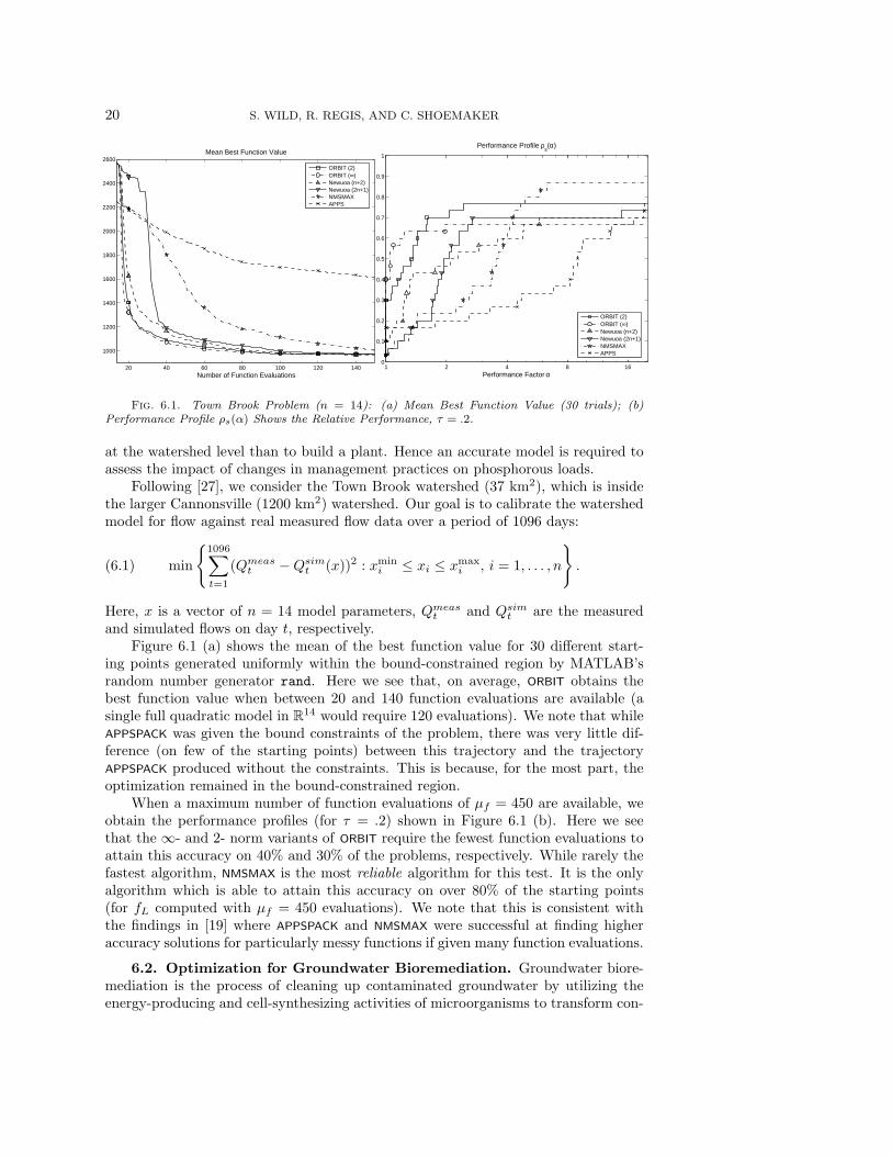
Fig. 6.1. Town Brook Problem (n = 14): (a) Mean Best Function Value (30 trials); (b)Performance Profile ρs(α) Shows the Relative Performance, τ = .2.

at the watershed level than to build a plant. Hence an accurate model is required toassess the impact of changes in management practices on phosphorous loads.

Following [27], we consider the Town Brook watershed (37 km2), which is insidethe larger Cannonsville (1200 km2) watershed. Our goal is to calibrate the watershedmodel for flow against real measured flow data over a period of 1096 days:

min

1096∑

t=1

(Qmeast −Qsim

t (x))2 : xmini ≤ xi ≤ xmax

i , i = 1, . . . , n

.(6.1)

Here, x is a vector of n = 14 model parameters, Qmeast and Qsim

t are the measuredand simulated flows on day t, respectively.

Figure 6.1 (a) shows the mean of the best function value for 30 different start-ing points generated uniformly within the bound-constrained region by MATLAB’srandom number generator rand. Here we see that, on average, ORBIT obtains thebest function value when between 20 and 140 function evaluations are available (asingle full quadratic model in R

14 would require 120 evaluations). We note that whileAPPSPACK was given the bound constraints of the problem, there was very little dif-ference (on few of the starting points) between this trajectory and the trajectoryAPPSPACK produced without the constraints. This is because, for the most part, theoptimization remained in the bound-constrained region.

When a maximum number of function evaluations of µf = 450 are available, weobtain the performance profiles (for τ = .2) shown in Figure 6.1 (b). Here we seethat the ∞- and 2- norm variants of ORBIT require the fewest function evaluations toattain this accuracy on 40% and 30% of the problems, respectively. While rarely thefastest algorithm, NMSMAX is the most reliable algorithm for this test. It is the onlyalgorithm which is able to attain this accuracy on over 80% of the starting points(for fL computed with µf = 450 evaluations). We note that this is consistent withthe findings in [19] where APPSPACK and NMSMAX were successful at finding higheraccuracy solutions for particularly messy functions if given many function evaluations.

6.2. Optimization for Groundwater Bioremediation. Groundwater biore-mediation is the process of cleaning up contaminated groundwater by utilizing theenergy-producing and cell-synthesizing activities of microorganisms to transform con-

ORBIT 21

20 40 60 80 100 120 140 160 180

104

105




1 2 4 80

0.1

0.2

0.3

0.4

0.5

0.6

0.7

0.8

0.9

1




Fig. 6.2. GWB18 Problem (n = 18): (a) (log10 scale) Mean Best Function Value (30 trials);(b) Performance Profile ρs(α) Shows the Relative Performance, τ = .01.

taminants into harmless substances. Injection wells pump water and electron accep-tors (e.g. oxygen) or nutrients (e.g. nitrogen and phosphorus) into the groundwaterin order to promote growth of microorganisms. We assume that sets of both injectionwells and monitoring wells, used for measuring concentration of the contaminant, arecurrently in place at fixed locations. The entire planning horizon is divided into man-agement periods and the goal is to determine the pumping rates for each injection wellat the beginning of each management period so that the total pumping cost is mini-mized subject to constraints that the contaminant concentrations at the monitoringwells are below some threshold level at the end of the remediation period.

In this investigation, we consider a hypothetical contaminated aquifer whose char-acteristics are symmetric about a horizontal axis. The aquifer is discretized using atwo-dimensional finite element mesh. There are 6 injection wells and 84 monitoringwells (located at the nodes of the mesh) that are also symmetric about the horizontalaxis. By symmetry, we only need to make pumping decisions for 3 of the injectionwells. Six management periods are employed, yielding a total of 18 decision variables.Since we are only able to detect feasibility of a pumping strategy after running thesimulation, we eliminate the constraints by means of a penalty term as done by Yoonand Shoemaker [31]. We refer to this problem as GWB18.

Figure 6.2 (a) shows the mean of the best function value for 30 different startingpoints again generated uniformly within the bound-constrained region by MATLAB’srandom number generator. Note that by the time the NEWUOA variant interpolating2n + 1 = 37 points has formed its first underdetermined quadratic model, the twoORBIT variants have made significant progress in minimizing the function. Also notethat since ORBIT is interpolating at up to 3n points, it is able to make greater progressthan the n + 2 variant of NEWUOA.

In Figure 6.2 (b) we show performance plots for τ = .01 with a maximum numberof function evaluations of µf = 570. Here we see that the ORBIT ∞-norm and ORBIT

2-norm are the best algorithms on 53% and 33% of the starting points, respectively.

7. Conclusions and Future Work. Our numerical results allow us to concludethat ORBIT is an effective algorithm for derivative-free optimization of a computation-ally expensive objective function when only a limited number of function evaluationsare permissible. More computationally expensive functions, simulating larger physical


domains or using finer discretizations, than the applications considered here wouldonly increase the need for efficient optimization techniques in this setting.

Why do RBF models perform well in our setting? We hypothesize that eventhough smooth functions look like quadratics locally, our interest is mostly in shortterm performance. Our nonlinear RBF models can be formed (and maintained) us-ing fewer points than full quadratic models while still preserving the approximationbounds guaranteed for linear interpolation models. Other nonlinear models with lin-ear tails could be tailored to better approximate special classes of functions, but theproperty of conditional positive definiteness makes RBFs particularly computation-ally attractive since we can include virtually as many evaluated points as desired. Ourmethod of adding points relies on precisely this property. Further, because we are notbound by linear algebraic expenses, the number of points interpolated can vary fromiteration to iteration and we can keep a complete history of the points available forinterpolation. Lastly, the parametric radial functions in Table 3.1 can model a widevariety of functions.

In the future, we hope to better delineate the types of functions which we expectORBIT to perform well on. We are particularly interested in determining whether ORBIT

still outperforms similarly greedy algorithms based on underdetermined quadraticmodels, especially on problems involving calibration (nonlinear least squares) andfeasibility determination based on a quadratic penalty approach. While we haverun numerical tests using a variety of different radial functions, to what extent theparticular radial function affects the performance of ORBIT remains an open question,as does the performance of ORBIT on problems containing areas of nondifferentiability.We also hope to better understand the computational effects of different pivotingstrategies in our method of verifying that a model is fully linear. We also intendto explore alternative methods for solving the subproblem since the current use ofFMINCON is both a large part of the algorithm’s overhead and currently limits ORBIT

from obtaining high accuracy solutions.

Lastly, we acknowledge that many practical blackbox problems only admit alimited degree of parallelization. For such problems, researchers with large scalecomputing environments would achieve greater success with an algorithm, such asAsynchronous Parallel Pattern Search [11, 15], which explicitly evaluates the functionin parallel. We have recently begun exploring extensions of ORBIT which take advan-tage of multiple function evaluations occurring in parallel and the presence of boundconstraints. Several theoretical questions also remain and are discussed in [29].

Acknowledgments. The authors are grateful to Raju Rohde, Bryan Tolson,and Jae-Heung Yoon for providing the simulation codes based on simulation codesfrom their papers [27] and [31] used by us here as application problems. We are alsograteful to Andy Conn, Jorge More, and two anonymous referees for their helpfulsuggestions.

REFERENCES

[1] M. Benzi, G. Golub, and J. Liesen, Numerical solution of saddle point problems, ActaNumerica, 14 (2005), pp. 1–137.

[2] M. Bjorkman and K. Holmstrom, Global optimization of costly nonconvex functions usingradial basis functions, Optimization and Engineering, 1 (2000), pp. 373 – 397.

[3] M. Buhmann, Radial Basis Functions: Theory and Implementations, Cambridge UniversityPress, Cambridge, England, 2003.

ORBIT 23

[4] A. Conn, N. Gould, and P. Toint, Trust-region methods, MPS-SIAM Series on Optimization,SIAM, Philadelphia, PA, USA, 2000.

[5] A. Conn, K. Scheinberg, and P. Toint, Recent progress in unconstrained nonlinear opti-mization without derivatives, Math. Programming, 79 (1997), pp. 397–414.

[6] , A derivative free optimization algorithm in practice, in Proc. of 7thAIAA/USAF/NASA/ISSMO Symp. on Multidisciplinary Analysis and Optimization,1998.

[7] A. Conn, K. Scheinberg, and L. Vicente, Geometry of interpolation sets in derivative freeoptimization, Math. Programming, 111 (2008), pp. 141–172.

[8] E. Dolan and J. More, Benchmarking optimization software with performance profiles, Math.Programming, 91 (2002), pp. 201–213.

[9] K. Fowler, J. Reese, C. Kees, J. J.E. Dennis, C. Kelley, C. Miller, C. Audet,

A. Booker, G. Couture, R. Darwin, M. Farthing, D. Finkel, J. Gablonsky, G. Gray,

and T. Kolda, A comparison of derivative-free optimization methods for water supply andhydraulic capture community problems, Adv. in Water Resources, 31 (2008), pp. 743–757.

[10] N. Gould, D. Orban, and P. Toint, CUTEr and SifDec: A constrained and unconstrainedtesting environment, revisited, ACM Trans. Math. Soft., 29 (2003), pp. 373–394.

[11] G. Gray and T. Kolda, Algorithm 856: APPSPACK 4.0: Asynchronous parallel patternsearch for derivative-free optimization, ACM Trans. Math. Soft., 32 (2006), pp. 485–507.

[12] H.-M. Gutmann, A radial basis function method for global optimization, J. of Global Opti-mization, 19 (2001), pp. 201–227.

[13] N. Higham, The Matrix Computation Toolbox. www.ma.man.ac.uk/~higham/mctoolbox.[14] T. Kolda, R. Lewis, and V. Torczon, Optimization by direct search: New perspectives on

some classical and modern methods, SIAM Review, 45 (2003), pp. 385–482.[15] T. G. Kolda, Revisiting asynchronous parallel pattern search for nonlinear optimization, SIAM

J. on Optimization, 16 (2005), pp. 563–586.[16] L. Linker, G. Shenk, R. Dennis, and J. Sweeney, Cross-media models of the Chesapeake

Bay watershed and airshed, Water Quality and Eco. Model., 1 (2000), pp. 91–122.[17] Mathworks, Inc, Optimization Toolbox for Use with MATLAB: User’s Guide, V. 3, 2004.[18] J. More, B. Garbow, and K. Hillstrom, Testing unconstrained optimization software, ACM

Trans. Math. Softw., 7 (1981), pp. 17–41.[19] J. More and S. Wild, Benchmarking derivative-free optimization algorithms, Tech. Report

ANL/MCS-P1471-1207, Argonne National Laboratory, MCS Division, 2007.[20] P. Mugunthan, C. Shoemaker, and R. Regis, Comparison of function approximation,

heuristic and derivative-based methods for automatic calibration of computationally ex-pensive groundwater bioremediation models, Water Resour. Res., 41 (2005).

[21] R. Oeuvray, Trust-region methods based on radial basis functions with application to biomed-ical imaging, PhD thesis, EPFL, Lausanne, Switzerland, 2005.

[22] R. Oeuvray and M. Bierlaire, A new derivative-free algorithm for the medical image regis-tration problem, Int. J. of Modelling and Simulation, 27 (2007), pp. 115–124.

[23] M. Powell, UOBYQA: unconstrained optimization by quadratic approximation, Math. Pro-gramming, 92 (2002), pp. 555–582.

[24] , Least Frobenius norm updating of quadratic models that satisfy interpolation conditions,Math. Programming, 100 (2004), pp. 183–215.

[25] , The NEWUOA software for unconstrained optimization without derivatives, in Large-Scale Nonlinear Optimization, Springer, 2006, pp. 255–297.

[26] R. Regis and C. Shoemaker, A stochastic radial basis function method for the global opti-mization of expensive functions, INFORMS J. of Computing, 19 (2007), pp. 497–509.

[27] B. Tolson and C. Shoemaker, Cannonsville reservoir watershed swat2000 model develop-ment, calibration and validation, J. of Hydrology, 337 (2007), pp. 68–86.

[28] H. Wendland, Scattered Data Approximation, Cambridge University Press, Cambridge, Eng-land, 2005.

[29] S. Wild and C. Shoemaker, Global convergence of radial basis function trust-region algo-rithms, In preparation.

[30] D. Winfield, Function minimization by interpolation in a data table, J. of the Institute ofMathematics and its Applications, 12 (1973), pp. 339–347.

[31] J.-H. Yoon and C. Shoemaker, Comparison of optimization methods for ground-water biore-mediation, J. of Water Resources Planning and Management, 125 (1999), pp. 54–63.

orbit: optimization by radial basis … optimization by radial basis ... a previous point must be...

Documents