multivariate hermite interpolation in euclidean space … · multivariate hermite interpolation in...

MULTIVARIATE HERMITE INTERPOLATION IN EUCLIDEAN SPACE

AND ITS UNIT SPHERE BY RADIAL BASIS FUNCTIONS

Thesis submitted for the degree of Doctor of Philosophy

at the University of Leicester

By

Zuhua Luo

Department of Mathematics & Computer Science University of Leicester

4 September 1998

UMI Number: U 594568

All rights reserved

INFORMATION TO ALL USERS The quality of this reproduction is dependent upon the quality of the copy submitted.

In the unlikely event that the author did not send a com plete manuscript and there are missing pages, th ese will be noted. Also, if material had to be removed,

a note will indicate the deletion.

Dissertation Publishing

UMI U 594568Published by ProQuest LLC 2013. Copyright in the Dissertation held by the Author.

Microform Edition © ProQuest LLC.All rights reserved. This work is protected against

unauthorized copying under Title 17, United States Code.

ProQuest LLC 789 East Eisenhower Parkway

P.O. Box 1346 Ann Arbor, Ml 48106-1346

A b s tra c t

In this thesis, we consider radial basis function interpolations in d-dimensional

Euclidean space and the unit sphere S d_1, where the data is generated not

only by point-evaluations, but also by the derivatives, or differential/pseudo-

differential operators. Some sufficient and necessary conditions for the well-

posedness of the interpolations are given. The results on sensitivity and sta

bility of the interpolation systems are obtained. The optimal properties of the

interpolants are analysed through the variational framework and reproducing

kernel Hilbert space property, the error bounds and convergence rates of the

interpolants are derived. The admissible reproducing kernel Hilbert spaces are

also characterised.

2

Preface

It is my pleasure to acknowledge the support I have received during my doc

toral research.

First, and foremost, my gratitude goes to Dr. Jeremy Levesley for his sup

port, intuition and patience whilst supervising my studies. As a m ature student,

I often stick to my own understanding and opinions stubbornly, and it takes

pains for him to get rid of my inappropriate ways of thinking. Many thanks for

his patience in correcting my writings, and for enduring the annoying arguments

because of my inability to listen. In particular, the great care he has exhibited

in reading my work will be of lasting benefit.

Special gratitude must go to Professor Will Light, who introduced me to the

research of radial basis function interpolation. W ithout the combined effort of

Will and Jeremy, I won’t be able to complete the study in Leicester. His encour

agement and breadth of knowledge in approximation theory and mathematics

has been of great help to me. In particular, it was Will who introduced me to

the beautiful variational theory.

Thanks must also go to Professor Ward Cheney and Xingping Sun. The

constant encouragement from Ward is invaluable, and so is his broad know

ledge of mathematics. This work has direct and close relation to the poineering

works which either Ward or Xingping authored. In particular, Xingping’s visit

to Jeremy in 1995 resulted in a method which eventually leads to one chapter

of this thesis. I would also like to thank Dr. Valdir Menegatto for generously

sending his papers to me which initiated my study on sphere.

3

There are other people whom I owe thanks. Certainly this work would not

have been possible without the support of the Overseas Research Scholarship

from the UK Committee of Vice-Chancellors and Principals, and a D epart

mental Scholarship from the Department of M athematics and Computer Sci

ence a t the University of Leicester. Finally, but of course not lastly, I owe my

gratitude to my family and friends. In particular, I thank my wife and daughter

for my happy life during the time. I am unable to thank my father, who died

before my leaving for Britain, and I have felt the loss keenly. This dissertation

is dedicated to the memories of my parents.

Contents

1 In tro d u c tio n 4

1.1 Radial basis function in te rp o la tio n ...................................................... 4

1 .2 Spherical radial basis function in te rp o la tio n ..................................... 8

1.3 Radial basis function Hermite in te rp o la tio n ...................................... 11

2 P re lim in a rie s for ana lysis 16

2.1 Distributions and Fourier transforms in ]Rd ...................................... 17

2.2 Spherical ana lysis ...................................................................................... 22

2.2.1 Distributions on 5 d _ 1 ................................................................ 22

2 .2 .2 Spherical h a rm o n ic s .............................................................. . 23

2.2.3 Sobolev spaces on 5 d _ 1 ............................................................. 26

2.2.4 Convolutions and Fourier analysis on 5 d _ 1 30

3 S tr ic tly co n d itio n a lly p o sitiv e d efin ite fu n c tio n s in lR d 35

3.1 In troduction ................................................................................................ 35

3.2 Integral rep resen ta tio n ............................................................................ 36

3.3 Criteria for r-C P D m and r-SCPDm functions in terms of Fourier

transfo rm s................................................................................................... 46

4 S tr ic tly co n d itio n a lly p o s itiv e d efin ite fu n c tio n s o n S d~1 50

4.1 In troduction ................................................................................................ 50

1

4.2 r-C P D m functions, and r-SC PD m functions in strong form . . . 53

4.3 Sufficient conditions for order N r-SPD fu n c tio n s .......................... 55

5 S ta b ility o f in te rp o la tio n in lRd 61

5.1 In troduction ............................................................................................... 61

5.2 The two a p p ro a c h e s ............................................................................... 63

5.3 The case r° , 1 < a < 2 ........................................................................... 64

5.4 Further remarks ..................................................................................... 72

6 S ta b ility o f in te rp o la tio n on 5 d _ 1 73

6.1 In troduc tion ............................................................................................... 73

6.2 Preliminaries and lem m as..................................................................... 74

6.3 Upper bound for ||^4—1 1|: The r-SPD and r-SC PD i cases . . . . 81

6.3.1 Lagrange in terpo lation ............................................................... 81

6.3.2 Hermite in te rp o la tio n ............................................................... 8 6

6.4 Lower bound for | | t / - 11 | ........................................................................ 8 8

6.5 Further remarks ..................................................................................... 92

7 T h e v a r ia tio n a l th e o ry 93

7.1 In troduc tion ............................................................................................... 93

7.2 The admissible s p a c e ............................................................................... 96

7.2.1 The case when G = K d ........................................................... 99

7.2.2 The case when G = 5 d _1 ........................................................... 1 0 2

7.3 Optimal interpolant and error estim ates.............................................. 105

8 C o nvergence r a te in ]Rd 112

8.1 In troduction .................................................................................................. 112

8.2 The technical l e m m a s ...............................................................................114

8.3 The main re s u lt ............................................................................................118

2

9 C o n v erg en ce r a te on S d~l 1 2 2

9.1 In troduction ..................................................................................................122

9.2 Convergence rate on the circ le ......................................................123

9.3 Convergence rate on 5 d_1, d > 2 ....................................129

B ib lio g rap h y 137

3

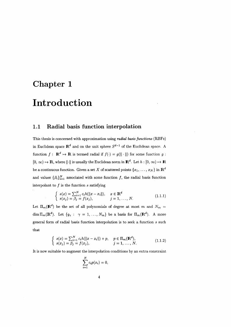
Chapter 1

Introduction

1.1 Radial basis function interpolation

This thesis is concerned with approximation using radial basis functions (RBFs)

in Euclidean space R d and on the unit sphere 5 d - 1 of the Euclidean space. A

function / : ^ K, is termed radial if /(•) = p(|| • ||) for some function g :

[0, oo) ]R, where ||-|| is usually the Euclidean norm in R d. Let h : [0, oo) h-» ]R

be a continuous function. Given a set X of scattered points {xi, . . . , xjv) in !Rd

and values {0i}^=l associated with some function / , the radial basis function

interpolant to / is the function s satisfying

J s (x ) = T,?=iCih (\\x -X i\\) , x e i R d n i nX s{x-j) = 0j = f { x j ), j = 1, . . . , N.

Let n m(]Rd) be the set of all polynomials of degree a t most m and N m =

d im n m(]Rd). Let {q7 : 7 = 1, . . . , N m} be a basis for IIm(]Rd). A more

general form of radial basis function interpolation is to seek a function s such

that

I s{x) = ah(\ \x - Xi||) +p, p e n m(]Rd), n i 21I s(xj) = (3j = f ( x j ) , j = 1, . . . , N.

It is now suitable to augment the interpolation conditions by an extra constraint

N

^ 2 CiP{xi) = 0,i= 1

4

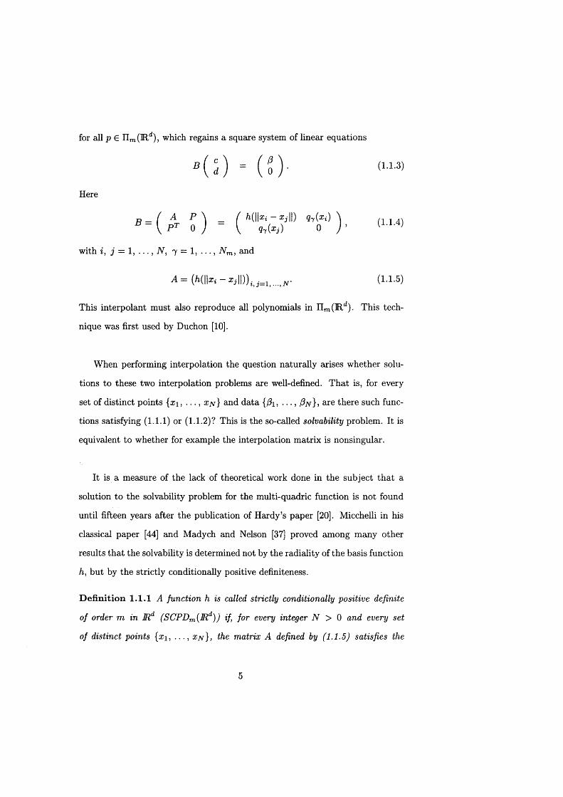
for all p G IIm(lRd), which regains a square system of linear equations

B ( d ) = ( o ) - (1'1'3)

B = l n ) = ^ ] , (1.1.4)

Here

P T 0 ) ~ \ q-y (x j ) 0

with i, j = 1, . . . , N , 7 = 1, . . . , N m, and

A = ( H W x i - X j W ) ) . . ^ ^ . (1.1.5)

This interpolant must also reproduce all polynomials in n m(lRd). This tech

nique was first used by Duchon [10].

When performing interpolation the question naturally arises whether solu

tions to these two interpolation problems are well-defined. T hat is, for every

set of distinct points { x \ , . . . , x/v} and data {fi\, . . . , Pn }, are there such func

tions satisfying (1.1.1) or (1.1.2)? This is the so-called solvability problem. It is

equivalent to whether for example the interpolation matrix is nonsingular.

It is a measure of the lack of theoretical work done in the subject th a t a

solution to the solvability problem for the multi-quadric function is not found

until fifteen years after the publication of Hardy’s paper [20]. Micchelli in his

classical paper [44] and Madych and Nelson [37] proved among many other

results th a t the solvability is determined not by the radiality of the basis function

h, but by the strictly conditionally positive definiteness.

D efin itio n 1 .1 . 1 A function h is called strictly conditionally positive definite

of order m in ]Rd (SCPDm (Md)) if, for every integer N > 0 and every set

of distinct points {xi, . . . , xjv}, the matrix A defined by (1.1.5) satisfies the

5

inequality

N

^ 2 C i C j h ( \ \ x i - X j \ \ ) > 0, i , j —1

whenever 0 ^ c = (ci, . . . , cn) is such that

N

Y,CiP(Xi) = 0, P e U m (Md).1=1

We denote SCPD0(Md) by SPD(Md) for simplicity.

D efin itio n 1.1.2 A set of points {rci, . . . , x n } is called Um (Md)-admissible if

p € Urn(Md) and p (x i) = 0 , i = 1, . . . , N implies p = 0.

Micchelli [44] and Madych and Nelson [37] showed th a t the interpolation sys

tem (1 .1 .1 ) is well-defined whenever h is strictly positive definite, or strictly

conditionally positive definite of order 1. More generally, we have

A sse r tio n 1.1.3 The system (1.1.3) is uniquely solvable if h is strictly condi

tionally positive definite of order m and that the interpolation points {rri, . . . , x n }

be IIm (Md)-admissible.

P ro o f

One can find this proof in either Micchelli [44] or Madych and Nelson [37].

However, since the arguments of the proof will be repeatedly used, we include

the proof here.

We need only prove th a t if, in the equation (1.1.3), f3 = 0, then the vector

c = 0 and d = 0. Assume (3 = 0. Then we have

P T c = 0, (1.1.6)

and

A c + P d = 0. (1.1.7)

6

Multiplying both sides of (1.1.7) by cT, we have

0 = cTAc + cTP d = c t A c ,

by (1.1.6). Since h is strictly conditionally positive definite of order ra, it follows

from Definition 1.1.1 th a t the only vector satisfying cTAc = 0 is the zero vector.

It then remains to prove th a t d = 0. By (1.1.7) again, with c = 0, we have

Pd = 0.

Let Q — dyqy . Then it follows that

Q (xi) = 0, for i = 1 , . . . , N.

By Definition 1.1.1, the polynomial Q = 0. Since qi, . . . , ^ is a basis for IIm,

it follows th a t d = (di, . . . , d^m) = 0 . ■

There are many papers concerning necessary and sufficient conditions for

strictly conditionally positive definite functions, among them are Micchelli [44],

Sun [61] and Guo et al [19] and the references therein. We will discuss them

further in Chapter 3.

Another im portant question in implementing the interpolation (1.1.1) and

(1 .1 .2 ) is the stability: if the interpolations (1 .1 .1 ) and (1 .1 .2 ) are solvable, how

sensitive are they to the perturbation of the function data {A }^? It is clear

th a t the sensitivity of the interpolation (1 .1 .1 ) or (1 .1 .2 ) is determined by the

spectral norm of the inverse of the interpolation m atrix (1.1.5) or (1.1.4). Ball

[3], Sun [60] and Baxter [6 , 7] have estimated the spectral norm of the inverse of

the interpolation m atrix (1.1.5) for some specific basis function h which is either

strictly positive definite or strictly conditionally positive definite of order 1 , some

of their results being optimal. However it is Narcowich and Ward [47, 48] who

obtained upper bounds for the norm of the inverse of the interpolation m atrix

for a class of strictly conditionally positive definite functions. The conclusion is

7

that the smoothness of basis function h and the least separation distance among

the interpolation points determine the upper bound of the spectral norm of the

inverse of the interpolation matrix. The smoother the basis function h, the less

stable the interpolants.

Perhaps the most im portant question of all for the interpolation systems

(1 .1 .1 ) and (1 .1 .2 ) is the error bound of the interpolant s to the actual function

being approximated. Together with stability, it determines the efficiency of the

interpolation schemes. A large amount of literature has been devoted to this

subject, among the recent ones are Madych and Nelson [37, 38], Wu and Scha-

back [65], Powell [51], and Light and Wayne [27, 29], with the earlier ones dating

back to as early as Duchon [10, 11], Meinguet [39], and even Golomb and Wein

berger [18]. Their techniques may vary, but the underlining theme follows the

so-called variational approach for interpolation. This powerful technique turns

the interpolation systems (1 .1 .1 ) and (1 .1 .2 ) into a minimization problem, and

has the advantage of deducing the error bounds with ease. The resulting con

vergence rate for the interpolations in terms of density of interpolation points

is proportional to the smoothness of the basis function h: the smoother the

function h , the higher order the convergence rate. Clearly, there is a trade-off

between stability and the convergence rate for the radial basis function interpol

ation, as observed by Schaback [53]: a stable interpolation scheme has a poor

convergence rate, and vice versa.

1.2 Spherical radial basis function interpolation

Let d(x, y) be the geodesic distance between the points x , y on the unit sphere

5 d_ 1 of the d-dimensional Euclidean space IRd. Given a set of data {(/3j, Xi) G

1R x 5 d _ 1 : i = l , . . . , n}, and a basis function h : 1R+ i-» 1R, consider the

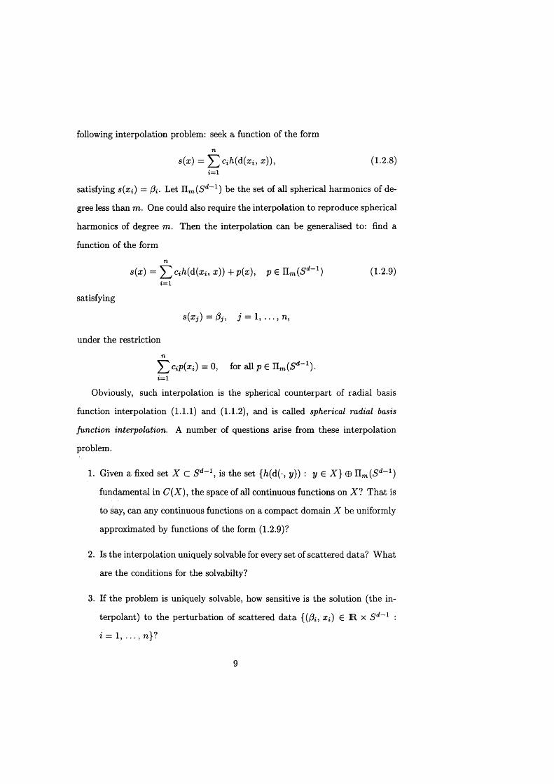
following interpolation problem: seek a function of the form

n

s (x ) = Y l Cih(d (Xi’ (1 .2 .8 )t=l

satisfying s(x{) = fy. Let IITO(S'd~1) be the set of all spherical harmonics of de

gree less than m. One could also require the interpolation to reproduce spherical

harmonics of degree m. Then the interpolation can be generalised to: find a

function of the form

n

s(x ) = ^ 2 Cih(d(xi, x)) + p(x), p G n m(5d_1) (1.2.9)1= 1

satisfying

8 (x j ) = P j , 3 = 1 ,

under the restriction

n

y ; Cip(xi) = 0, for all p G n m(5d_1).i - 1

Obviously, such interpolation is the spherical counterpart of radial basis

function interpolation (1 .1 .1 ) and (1 .1 .2 ), and is called spherical radial basis

function interpolation. A number of questions arise from these interpolation

problem.

1. Given a fixed set X C 5 d_1, is the set {h(d(-, y)) : y G X } © IIm(5 d_1)

fundamental in C (X ), the space of all continuous functions on X ? T hat is

to say, can any continuous functions on a compact domain X be uniformly

approximated by functions of the form (1.2.9)?

2. Is the interpolation uniquely solvable for every set of scattered data? W hat

are the conditions for the solvabilty?

3. If the problem is uniquely solvable, how sensitive is the solution (the in-

terpolant) to the perturbation of scattered data {(Pi, Xi) G R x S'd~1 :

i = 1 , . . . , n}?

9

4. How rapidly does the interpolant converge to the actual function being

approximated if the set of interpolation points becomes more dense?

It turns out th a t the answer to the above questions depends on the property of

the basis function h being strictly conditionally positive definite of order m on

the sphere.

D efin ition 1.2.1 A function h : M+ -» M is conditionally positive definite of

order m on 5 d _ 1 if, for every integer N > 0 and every set {X \ , . . . , a;at} C 5 d_1,

N

Y CiCjh(d(xi, Xj)) > 0 , (1 .2 .1 0 )i,j=l

whenever the coefficients C\, . . . , cn satisfyn

5 3 Cip(xi) = 0 ,i— 1

for allp € n m(5 d_1). I f the inequality (1.2.10) is strict then we say h is strictly

conditionally positive definite of order m on 5 d_ 1 ( or SCPDm (S d~1) for short).

I f m = 0 we say h is strictly positive definite on the sphere (or SPD (Sd~1) for

short).

D efin ition 1.2.2 A set {x i, . . . , x/v} C S d~l is n m(5 d_1)-admissible if the

only p G n m(5 d_1) satisfying p(x{) = 0 for i = 1, . . . , N is the zero polynomial.

By the same arguments in the proof of Assertion 1.1.3, it is easy to see th a t

the interpolation (1.2.9) is uniquely solvable, providing th a t h is SCPDm(5'd_1)

and the set {xi, . . . , xat} is Um (Sd~1)-admissible.

Schoenberg [55] showed th a t every positive definite function h on .Sd - 1 is

necessarily of the formOO

h(t) = ' y h kpjeX\c o s t ) , t e [ - 7 T , 7r], (1.2.11)k=o

with hk > 0 for A; > 0, where PkX\ A = (d — 2)/2, is the Gegenbauer poly

nomial of degree k. Xu and Cheney [6 6 ] and Ron and Sun [52] proved th a t if

10

the number of zero coefficients hk is finite then h is strictly positive definite.

Sun and Cheney [62] showed th a t if all the coefficients hk ^ 0, then the set

{h{d(-, y)) : y G S d-1} is fundamental in (7(Sd-1). Levesley, Luo and Sun

[25] and Luo and Levesley [33] obtained the bounds of condition number for

interpolation (1.2.9). The efforts of Levesley, Light, Sun and Ragozin [24], von

Golitschek and Light [15], Dyn et al [12], and Luo and Levesley [34] established

the variational framework for such spherical radial basis function interpolation,

giving rise to the results on error estimates and convergence rates of the in

terpolation on the sphere, the optimal properties of the interpolant, and the

construction and characterization of the admissible function space on which the

interpolant has the optimal properties.

1.3 Radial basis function Hermite interpolation

The main purpose of this thesis, however, is to generalize the above results to

Hermite interpolation in lRd and on 5 d_1. In many practical situations, such as

applying radial basis function or spherical radial basis function to solve partial

differential equations or pseudo-differential equations numerically, one often has

to use data generated by derivatives or derivative operators. This gives rise to

the necessity of studying Hermite interpolation using radial basis function and

spherical radial basis function.

We note that, in determining the solvability of interpolations, the key role

is played by the property of strictly conditionally positive definiteness of the

basis function h, not by the radiality or geodesic radiality of h. Hence in the

following, and throughout the thesis, we will assume th a t the basis function h

is conditionally positive definite.

11

Let G denote a domain in ]Rd and C( G) (respectively C 2r{G)) be the set

of continuous (respectively 2 r-tim es differentiable) real valued functions on the

domain G. Let £ ' be the dual space of C T(G). Let h £ C 2 t(G x G). Let us

assume th a t IIm is the set of polynomials of degree less than m on G. Let 8'm T

be the subset of £ ' whose elements annihilate IIm. For L £ S'T and / £ C T(G),

the operation of L on / is denoted by

[L, f)

and the convolution

L * h (x) = [L, h(-, x)].

The explicit meaning of distributional operations and convolutions will be ex

plained in details later.

D efin ition 1.3.1 Let the set of distributions A = {L i, L m } C The

radial basis function Hermite interpolant to f £ C T(G) is a function of the

form

N

s :='Y^/ ci L i * h + p, p £ IIm, (1.3.12)i— 1

where Y^iLi ci^ i ^ £'m,T> subject to the interpolation conditions

[L,s] = [ L , f \ , L e A.

When the distributions L i, . . . , L n are point evaluation functionals, and the

function h(x, y) = h(\x — y |) or h(x, y) = h(d(x, y)), the Hermite interpolant

becomes the usual radial basis function or the spherical radial basis function

interpolant discussed in Sections 1 .1 or Section 1 .2 , respectively.

12

W ith reference to the above definition, A is n m-admissible if A(p) = 0 for

all p G n m implies p = 0. Note also that we recover the usual interpolation

problem if all of the elements of A are point evaluation functionals.

D efin itio n 1.3.2 A function h : G x G M is called T-CPDm on G if for

every positive integer N , every set of distributions A = {L \, . . . , Ljv} C Z'T, the

inequality

N

CiCj[Li, L j * h] > 0 (1.3.13)j= l

holds whenever c = (c i, . . . , c/v) satisfies

N

^ 2 ci[L i> P) = °> f or P ^ n m-i= 1

I f the above inequality (1.3.13) is strict whenever Y2iLi°iLi i^ 0 annihilates

n m, then h is called T-SCPDm .

Similar to Assertion 1.1.3, we see that the radial basis function Hermite inter

polant defined above is uniquely solvable whenever h is r-SC PD m and the set

A is n m-admissible. Chapter 3 and Chapter 4 therefore discuss the conditions

for a radial basis function to be r-SCPDm in H d and on 5 d_1, respectively. In

Chapter 3, we first characterize the integral form of a r-SC PD m function in R d,

and then obtain a criteria for a function to be r-SCPDm according to its Fourier

transform. In Chapter 4, we first give a characterization of r-SC PD m functions

on S d~1 in its strong form, and then present several sufficient conditions for a

function to be r-SC PD m on S d~1 under various interpolation assumptions.

A large part of the thesis investigates the sensitivity of radial basis function

Hermite interpolations to the changes in the interpolating data. This study is

motivated by the observations that large condition numbers occur in practical

13

calculations using radial basis function. Two distinct approaches are analysed to

get the upper bounds on the spectral norm of inverses of interpolation matrices.

In Chapter 5, we use the approach similar to Ball [3] and Sun [60] to bound

from above the spectral norm of inverse of interpolation m atrix

{ \ \x i -X j \ \a) " j= v (1 < a < 2)

as tight as possible. Numerical tests show th a t the bound is much better than

that obtained by using the approach of Narcowich and W ard’s [48]. In the spe

cial case of a = 1 and dimension d = 1, the bound is sharp. In Chapter 6 ,

we use its analogous discrete form to get the upper bounds of spectral norms

of inverses of interpolation matricies for a large class of functions, namely the

r —SCPDi and r —SPD functions on 5 d~1. The estimating bounds are much

better than those obtained using the other approach by Narcowich, Sivakumar

and Ward [46] in the case of Lagrange interpolation when the Fourier coefficients

of the spherical radial basis function are of polynomial decay. We then use the

best approximation technique from Schaback [54] to get the lower bounds for

the spectral norm of the inverses of the Hermite interpolation matrices for all

r-SC PD m functions on 5 d_1.

The biggest part of this work is on error bounds and convergence rates of

the radial basis function Hermite interpolation in and on S d_1 respectively.

We begin in Chapter 7 with the variational approach proposed by Madych and

Nelson [37, 38] in a more general way to allow Hermite interpolation. Such a vari

ational approach for interpolation has its predecessors dating back to Duchon

[10], Meinguet [39] and to as early as Golomb and Weinberger [18]. Through

this approach, we prove that the radial basis function Hermite interpolant is

the optimal solution minimizing the semi-norm || • H* (the energy norm) among

the interpolants from the semi-Hilbert space (C/i,|| • ||/i), where (Ch, || • IU) is

14

determined by the r-SC PD m function h, and is termed the admissible space.

We then give a characterization of the admissible space Ch , and show th a t it is

equivalent to the weighted Sobolev space when the domain is R d or the sphere

5 d_1. Through the reproducing kernel Hilbert space theory, the error bounds

of the radial basis function Hermite interpolant is naturally obtained.

Based on the error estimation in Chapter 7, the convergence rate of radial

basis function Hermite interpolation in R d is discussed in Chapter 8 . It gen

eralizes the works of Madych and Nelson [38] and Wu and Schaback [65] to

include the Hermite interpolation, and contains the previous results as special

cases. The convergence rate analysis of interpolation on S d~1 turns out to be

more complex and delicate, and we divide it into two parts. In the first part

of Chapter 9, we analyse the convergence rate for Hermite interpolation on the

circle, and then in the second part discuss the convergence ra te of radial basis

function Hermite interpolation on 5 d_1, d > 2.

As the theoretic foundation of the thesis, in Chapter 2 we introduce some

notations and theories on distributions, convolutions and Fourier transforms in

R d, and the analogous discrete form counterpart on 5 d_1. Most of the notations

and theories here are from Donoghue [9], Gel’fand and Vilenkin [16] and Muller

[45].

15

Chapter 2

Prelim inaries for analysis

We work in d dimensional space ]Rd and on its unit sphere S d~1. Throughout the

thesis, we use the following notations. If a = (au, . . . , ad) and f3 = (fii, . . . , fid)

axe multi-indices, then

(1 ) M == Z U “ ii

(2 ) a! = a i! • • -ad!;

(3) D<* = D f 1 • • • D add, where Dj = d

(4) a < (3 means a j < (3j for 1 < j < d;

(5) a + 0 = (a i + 0i, . . . , ad + 0d), and a - (3 = a + (-/?) for a > (3;

(6 ) ± * = x ? - x * ‘ .

Let x, £ € lRd, / be a function, and R be a distribution defined later. Then

(7) x £ = x if i + . . . + x dU,

(8) / - (• ) = / ( - • ) ;

(9) 0] = [R, 0 (—)], for each suitable test functions 0.

16

2.1 Distributions and Fourier transforms in JRd

For a natural number r > 0, let C T(]Rd) denote the class of function in ]Rd

having continuous derivatives up to and including to tal order r . Let C(lRd)

denote the class of continuous functions and C°°(]Rd) the class of infinitely

differentiable functions in R d, respectively. Let Supp/ denote the closure of a

subset of R d on which the function / is nonzero. If Supp/ is a bounded set

of R d, then / is called a compactly supported function. Let C o (R d), C o (R d)

and Co°(]R,d) denote the subsets of C r (R d), C (R d) and C °°(R d), respectively,

whose elements axe compactly supported in R d. For convenience, we use V and

£ to denote the set C o°(R d) and C°°(]Rd), respectively. We call the elements

of V the test functions. We also use

V T and £t

to denote the sets

C 5(R d) and C T(lRd),

respectively. Let J denote a subset of £ whose elements rapidly decay at infinity,

i.e., if / G J , then for every integer m > 0 and every index a ,

(1 + \x\2)mD af (x) —► 0 as x -» oo.

D efin ition 2.1.1 A linear functional T on V is called a distribution i f and

only if for every compact set K C Md, there exist a constant C > 0 and integer

N > 0 such that

ItT, 4>]\ < c Y , I I ^ I U|a |< J V

for all (j) £ T> having compact support in K . Here || •H oc denotes the maximum

norm in JRd. I f the integer N can be chosen independently of the compact set

K , and N is the smallest such choice, then the distribution is said to be of order

17

N .

Let V denote the space of all continuous linear functionals on V, i.e., the dual

space of V. Similarly, let

£', £'r , V'T and J ' (2.1.1)

be the duals of

£, £t , V T and J ,

respectively. Obviously the following relations

V C V T C £r , £ C £r , (2.1.2)

D C J C f , (2.1.3)

and

£'T C V 'T C V , £'t C £', (2.1.4)

£ ' C J ' C V ' , (2.1.5)

are true. Besides, V is dense in J . Thereafter, we call the elements from

£ ', V , J ' , £'t and V'T distributions, and elements from £, £>, J7-, £T and V T test

functions. The elements from the space J ' are called tempered distributions,

[9, pl34]. It is well-known th a t the space £' consists of compactly supported

distributions; the space V'T consists of distributions of order at most r; and the

space £'t consists of compactly supported distributions of order at most r . We

denote by

the operation of a distribution T on a test function (f> from the corresponding

dual space.

18

Let L 1 (H d) denote the set of functions integrable in ]Rd. For each / G

L 1 (]Rd) , define the Fourier transform

r m = m ■■= ^ / R d / ( x ) e - ^ x .

The inverse Fourier transform Jr~1f is defined by

( ^ / > ( * ) ==

For / , <7 G L 2(]Rd), we also use ( / , g) to denote their inner product, i. e.,

{ f ’ 9) =

Clearly, the spaces V and J are subsets of L 1 (]Rd), hence their elements

have well-defined Fourier transform. In particular, the Fourier transform maps

J onto itself, and maps V into J . We denote by K the image of V under T .

Thus

K = T (V ) C J .

The Fourier transform T of a distribution T G J ' is defined via

[f , 0] = [ r ,0 ] , V 0 G *7, (2-1.6)

see Gelfand [17, pl90]. Likewise, the Fourier transforms T and S of distributions

T G S' and S G V are defined via

[ T j \ = [T ,0 ], V 0 g £ ,

and

[ S j ] = [5 ,0], V 0 G Z>.

The tempered distribution space J -' is invariant under the Fourier transform,

see e.g. [9, Section 30]. When T G S'T, the Fourier transform T is

f ( € > = W ^ [T’ e~i i l (2-L7)

19

satisfying

i T ( f l i < c ( i + K i r ,

for some constant C > 0; see [9, p!48].

(2 .1 .8)

The convolution / * g of two functions / , g € L 1 (IIId) is

f * 9{x] = ( d j ^ J f f f{y)9{x ~ v)dy■ (2-L9)

The convolution T * (j) of a distribution T £ J ' and a test function (f> is defined

via

(T * (f>)(x) = [T, (p(x - •)]. (2.1.10)

If T is a compactly supported distribution and 5 is tempered, then their con

volution T * S is well-defined [16, pl48]. We summarize some useful formulas

here for future use.

Lem m a 2.1.2 LetT, R be compactly supported distributions and S be tempered.

Let f , g £ J . Then

= f g ,

? { T * S ) = TS,

and

[ T * R ~ , f \ = [T, R * f ] . (2.1.11)

Moreover, T * / G J .

Rem ark 2.1.3 The equation (2.1.11) is valid whenever both sides of the equa

tion are well-defined.

20

For details of the above results, see [9, pl51] and [16, p l38 and pl48].

The following three classical theorems will be repeatedly used in the sequel;

see [8 , p293-p295] and [9, p35-p36] for more general forms.

T heorem 2 .1 .4 (Lebesgue Dominated Convergence Theorem) Let / i be a Le-

besgue measure on Md. I f a sequence /„ of integrable function on JRd converges

almost everywhere to f and if there exits an integrable function g such that

\fn\ < 9 almost everywhere for all n, then

lim / f n(x)dfx(x) = / f(x)dfi(x).n^ °° JM J m

T heorem 2.1.5 Let ^ be a Lebesgue measure on lRd. Let integer n > 0. A s

sume that the function f : Md x Md y-t M satisfies

(V / ( ’) y) £ C n (]Rd) for almost every y G Md,

(ii) D*ff{x , y) belongs to L l {|/z|) as a function o fy for every index a satisfying

M 5: n >

(Hi) there exists a function ga e L x{|ju|) such that

\Daf ( ; y ) \ < g a (y)

for every index a such that |a | — n.

Then the function

F(x) = J f (x, y ]M y ) e C ” ^ ) ,

and for every index a satisfying |a | < n,

D Z F (x )= f D 2 f { x , y ) M v ) ,JIR

holds for every x E M d.

21

T heorem 2.1 .6 (Approximation Theorem,) Let 0 G V such that 0(0) = 1. Let

& (*) = ^ ( f ) , < > 0 ).

Then for each continuous function f G C (Md),

f ( x ) = lim / * (x) . (2 .1 .1 2 )<5—H)

2.2 Spherical analysis2.2.1 Distributions on 5 d_1

A function / is infinitely (T-times) continuously differentiable on S d~1 if it can

be extended to an infinitely (r-times) continuously differentiable function in R d.

Let £ (S d_1) denote the class of functions on S d_ 1 whose elements are infinitely

continuously differentiable on Sd_1. Similarly, let C T(5 d_1) denote the class

of functions on S d~1 whose elements are r-times continuously differentiable on

S ' 1' 1 .

Let £ '( 5 d-1) be the dual of £ (5 d_1), i.e., the continuous linear functionals

on £ (5 d_1). Similarly, let £!r(S d~1) be the dual of C r (5 d_1). Every distribution

T G £ /(5 d_1) can be viewed as a distribution on R d, say T, via the identity

[ f ,0 ] := [T ,0 |s --i], (2.2.13)

where 0 |sd-i is the restriction of 0 on 5 d _1 and is in £ (5 d_1). Obviously T is

supported on 5 d_1. However, not every distribution supported on the sphere

comes from a distribution in £ /(S'd~1), for example the distribution T in £'(]Rd)

defined by

P’ i = £ ( 1>° °)involves a derivative in a direction perpendicular to 5 d _ 1 and so cannot be com

puted in terms of the restriction 0 |5 d-i. See [58, p99-102] for detailed discussion

22

of distributions on the sphere.

Every point x = ( x i , . . . , Xd) G S d 1 can be expressed by its polar coordin

ates (0i, . . . , 0d_i) G @ d _ 1 via

where

x \ = sin 0 i ,X2 = cos 0 i sin 0 2 ,

Xd- 1 = cos 0i • • ■ cos Qd- 2 sin 0<*_ i ,k Xd = COS 0i • • ■ COS 0d—2 COS 0d—l ,

©d 1 ;= [0, 27r) x • • ■ x [0, 27t) x [0, 7r).

(2.2.14)

Let

d

(2.2.15)

(2.2.16)

For a suitable smooth function / : S d~l h>R, 0 6 0 d _ 1 and its corresponding

point xe G 5 d_1, the following holds,

d.= E a« w

d f ( x 0)d 0 . ^ Q x >

3= 1 J

(2.2.17)

where dij{0) are trigonometrical polynomials of 0. Hence for an index a =

(& 1 , . . . , OCd— 1),

D ? f M = E b m i f M ,0 , 1 < p < oo,

23

where d/j, is the rotation invariant probability measure on 5 d 1. For / , g G

L2^ " 1), let

(/> 9) = [ fU d v (2.2.19)JSd~ 1

be their inner product. This inner product induces a norm || • U2 for L 2 (Sd_1).

Let n (5d_1) be the space of spherical polynomials on S d-1. Let n m(5d_1)

be the subspace of spherical polynomials of degree no greater than m on 5 d_1.

Let

n^ = E„(S‘|- 1) n n m_1(S'i- 1)1 ,

be the set of homogeneous spherical harmonics of degree m, where IIm_i (5'd-1)J-

denotes the orthogonal complement of n m_i(Sd-1) in spherical polynomial

space II(Sd_1). Let

dk = dim(n») = {2k + d - » % ; d - > )]. (2.2.20)

See Muller [45] for reference. It is obvious that dk = 0 ( k d~2).

Let . . . , Yk,dk} be an orthonormal basis for 11 with respect to the

inner product (2.2.19). It is well-known that 11® is a space of eigenfunctions

of the Laplace-Beltrami operator A* on S d~1 with respect to the eigenvalue

A* = — k(k + d — 2): for every Y € 11°,

A *y = A*F. (2.2.21)

The exact form of the operator A* is unimportant for the thesis.

The spaces II® and II® are orthogonal with respect to the inner product

(2.2.19) for k ^ j \ 11* is the direct sum ©*_0 II®. See [45] for more details.

Every continuous function F on 5 d_ 1 has a formal harmonic expansion

00 dk

E E V u .k=0 j = 1

24

where

Fk,j — f F Y k j dfi.Jsd~1' S d -

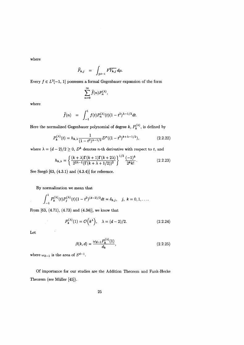
Every / G L 2[— 1, 1] possesses a formal Gegenbauer expansion of the formOO

£ f ( n )PnA)’n = 0

where

m = 1 1 f ( t ) p ^ m - t y - ^ d t .

Here the normalized Gegenbauer polynomial of degree k, p j ^ , is defined by

P ? \ t ) = hk,x (1 _ <2X _1/2 P"(( 1 - (2.2.22)

where A = (d — 2)/2 > 0, D k denotes n-th derivative with respect to t, and

f (A + A)r(fc + i)r(fc + 2 A) l 1 /2 ( - i ) fc \ 2 2A- 1 (r(fc +A + l / 2 ) ) 2 J 2 kk\ ‘

See Szego [63, (4.3.1) and (4.3.4)] for reference.

By normalization we mean that

£ p i A> (t)p f> (t)( i - t2Y d~ ^ 2dt = st J , j , k = o ,i , . . . .

From [63, (4.71), (4.73) and (4.34)], we know that

Pjix\ l ) = 0 ( k xy \ = (d — 2)/2. (2.2.24)

Let

/? (M ) = Wd- lPJ ~ )l-X\ (2.2.25)dk

where u<i-i is the area of S d~l .

Of importance for our studies are the Addition Theorem and Funk-Hecke

Theorem (see Muller [45]).

25

L em m a 2.2.1 Let Y k j be an orthogonal basis for 11 , the Gegenbauer

polynomial of order k, and f € L2 [—1, 1]. Then we have the Addition Formula,

l f \ x y ) = (2.2.26)3= 0

and the Funk-Hecke formula,

[ f (x y )Y n>l(y)dp(y) = p (k ,d ) f(n )Y n>l(x). (2.2.27)Jsd~1

By the Addition Formula (2.2.26), every F G L 2(S d~1) has a formal spherical

harmonic expansion,oo „

£ ( /? ( * , d) ) ' 1 / F (y )P ^ (x y )d M(y). (2.2.28)

2.2.3 Sobolev spaces on S d ~ l

We define, for r > 0, the weighted Sobolev space H r{Sd~ l ) on by

oo dk

F r (5 d" 1) := { F : 5 d- 1 i -> R | X ^ S l ^ > J ' |2(l + A:)2r’ < o°}- (2-2-29)*=o j = 1

Its dual is the distribution set H ~ r(S d~1) defined by

oo dk

H - ’-(Sd- 1) := { L | ^ ^ ^ / ( l + i O - ^ c o o } , (2.2.30)k=0 j=l

where

Lk,j = ^k,j]

is the value of the distribution L on the harmonic Y k j. On these spaces, we

introduce the inner products and norms in the obvious way,

oo dk _____

and

(F, G)r = £ £ i = V A i ( l + l f r, V F , G € f l f (S1- 1),A:=0 j= 1

(L,T)_r = ^ ^ X t j f w (l + J:)-2r, VL, T e / f - ’-fS""1).A:=0 j=1

26

For / £ i? r (5 d_1) and L £ H ~ r (S d~1), the operation of the distribution L on

the function / ,

OO d n

[-^ / ] = y i Lk,jfk,j,k = 0 j = 1

is absolutely convergent and hence is well-defined.

T heorem 2.2.2 For r > (d - l) /2 , i7r(Sd_1) is a subspace o /C (S d_1).

P ro o f

Let / £ f f r’(5 d-1) with r > (d — l) /2 . By the Cauchy-Schwarz inequality and

the addition formula (2.2.26),

oo dfc

fc=0 j = l

/ oo dfc

^ ( E E i * j i 2(1 + i )2r

= i i / i i J E ( d * K - 1) ( i+ f c ) - 2’-\fc=o

By (2.2.20), d* = 0 (fc(d" 2)). Thus

OO OO

E(d‘/ -')(1 + fc)“2’' CE(l + *:)_2r+(‘i‘2) < 00,/e= 0 fc=0

as r > (d — l) /2 . Hence / is continuous and has an absolutely convergent

spherical harmonic expansion. ■

One important concept for our investigation of Hermite interpolation on the

sphere is that of a pseudo-differential operator.

D efin itio n 2.2.3 We call $ a pseudo-differential operator with symbol { $ k , j , k =

0 , 1 , . . . , 1 < j < dk} if and only if, for all spherical harmonics Y k j, 1 < j <

dki k ^ 0 ,

* (Y k j) = * k jY kj (2.2.31)

27

holds. Furthermore, if there exist positive constants C\ and C2 a,nd m > 0 such

that for k > 0 ,

Cikm < \ * kJ\ < C 2km,

then the pseudo-differential operator $ is said to be of order m .

Obviously the Laplace-Beltrami operator A* is of order 2; see (2.2.21).

Lem m a 2 .2 .4 I f $ is a pseudo-differential operator of order s < r and f €

i J r (5 d_1), then g = $ ( / ) € F r - S(5 d" 1).

P ro o f

We need only prove that

00 dk

£ £ i w 2(i + * )2<’- ’> < 0°.k= 0 j = 1

Note that, g = $ ( / ) has a formal spherical harmonic expansion of the form,

00 d k 00 dk

k=0 j=l k=0 j —1

Thus

\9k,j\ = \ f k , j $k , j \ <( l + k)8\fk J \,

and therefore we have

00 dk

£ Z > j l 2(i + *)s(r-* )k=0 j=1

00 dk

^ c £ £ + *)2r = c ii/ ii? < °°-fc=o j = 1

This completes the proof. ■

Combining with the previous theorem we get

T heorem 2.2.5 For r > r + ( d — l) /2 , H r (S d~1) is a subspace o fC T(S d~1).

28

Let 8X be the point-evaluation distribution a t x G S d 1.

T h eo rem 2.2.6 Let $ be an pseudo-differential operator of order m . Let L

8X o $ . Then L belongs to H ~ r(S d~1) if r > m + (d — l ) /2 .

P ro o f

Note th a t L has a formal spherical harmonic expansion

oo dk

Jfe=0 1=1

where L kyi = [6X o $ , Yk,i] = $ k,iYkti(x) with

C ik m < < C2km.

Hence we have

oo dk

E E i £ w ia( i + * r 2“k=0 1=1

oo dk

= E E i * w i 2 iy*.‘i2 (1 + * r 2“k=o 1=1

oo dk

A:=0 1=1 oo

< C 2 ^ ( d , / w <(_ 1)(l + i:) - 2“+2’"k= 0

-2a

< c 2 £ > + *)-\ —2a+(d—2)-f 2m

k= 0

In the penultimate inequality we have used the Addition Formula (2.2.26). The

sum is convergent if —2 a + (d —2) + 2m < —1 , or equivalently, a > m + (d —1 ) / 2 .

■

As a consequence, we have

T h eo rem 2 .2 .7 The distribution 8X belongs to H ~ r (S d~1) if r > ( d — l ) /2 .

29

2.2.4 Convolutions and Fourier analysis on S d 1

A function of the form Fy(x) = f ( xy) , f : [—1,1] *-> H , y £ S d~ 1 is termed

zonal, since F is invariant under any rotation which fixes y. For / £ L 2 [—1, 1],

and G 6 L 2(S d~1), we define their convolution by

( f * G ) { x ) = [ f(xy )G (y )d y . (2.2.32)J s ^ 1

If in particular, both / and g axe elements of L2[—1, 1], then we have a convo

lution of two zonal functions defined by

( f * g ) ( x z ) = [ f (xy)g{yz)dy. (2.2.33)Js*-1

The convolution of any two zonal functions is itself zonal. See [45, p. 19] for

the proof. In fact, for / , g £ L 2[— 1, 1], there exists h G L 2[—1,1] such th a t

h = f * g. It is easy to see that the convolution in (2.2.33) is commutative, i.e.,

f * g = g * f .

T h e o re m 2.2.8 Let f , g £ L 2[— 1, 1], and le th = f * g . Then h has the formal

Gegenbauer expansion

OO

£ £ n P ,< A),n=0

with

h(n) = 0(n ,d)f{n)g{n),

where /3(n,d) is defined by (2.2.25).

P ro o f

Choose a Yn £ 11° and x G 5 d - 1 so that Yn(x) 0. Applying the Funk-Hecke

formula 2.2.27 first to h and then to g and / respectively, we have

fi(n ,d)h(n)Y n ( x) = [ h(xy)Yn (y)dy J s d~1

30

- ( / f ( x z ) g ( y z ) d z ) Y n (y)dyJ s d- ' \ J s J

= [ f {xz ) f [ g(yz)Yn (y) d y ) dzj Sd-1 KJs*-1 J

- fi(n,d)g(n) [ f ( x z )Y n (z )d zJ s d~ i

= 0(n, d) 2 g(n)f{n )Y n {x),

which proves the theorem. ■

Similarly, we have

T h e o re m 2 .2 .9 Let f G L 2[ - 1, 1], G G L 2 (5 d“ 1) and let F = f * G . Then F

has a formal spherical harmonic expansionoo dk

E E w .fc=o i=i

with

Fk,j = (3(k,d)fkGkj .

Now let us look at the convolution of a distribution L on the sphere with a zonal

function. Let h G L 2[— 1, 1]. Then

L * h(x) = [L, h{x •)], x G S d~ \ (2.2.34)

is the convolution of L with h.

T h e o re m 2.2.10 Let h have a formal Gegenbauer expansionOO

(2-2.35)k=0

such that

hk = o ( ( l + k)~sl3 (k ,d )-i y (2.2.36)

Then for each L G H ~ r(Sd~1) with r < s, L * h G H s~r (S d~1). Moreover, the

Fourier coefficient of the Gegenbauer expansion for L * h is

fi(k, d)hkL kj .

31

P roof

Let g = L * h . Then g has the spherical harmonic expansion

oo dkY , h k m d ) £ [ l , n j ] n , i ( x )k=o j = 1

oo dk= ^ 2 Y L 9 k ,jY k>j(x),

k=0 j = 1

with

Thus

oo dkEE&;i!(i+i)2(- r>k=0 j=l

oo dfc _____2

= E E d)£ * j (x+*)2<s_r)fc=o j=l oo dfc

<EEi£ i2(1+*r2r<“’fc=0 j=1

where in the last two inequalities, we have used (2.2.36) and the fact th a t

L £ H ~ r(Sd~l ). Thus by the definition of F r (5d“ 1), g € ■

We then immediately have

C o ro lla ry 2.2.11 Under the assumptions on h of Theorem 2.2.10,

[L , T * h ]

is well-defined for all L £ H ~ r(Sd~1) and T £ iy - t (5 d-1) with r + t < s.

C o ro lla ry 2.2.12 Under the assumptions on h of Theorem 2.2.10, for every

fixed point x £ 5 d_1, the following statements are true.

1. The function h{x •) £ H s~r for all r > (d - l) /2 .

2. The function h(x •) is continuous if s > (d — 1).

32

3. The function h(x •) is m-times continuously differentiable whenever s >

(d — 1 ) + m.

P ro o f

Note that the point evalution distribution Sx is in the space H ~ r for r > (d —

l ) /2 . Hence by Theorem 2.2.10, h(x •) is in H s~r . This proves the first assertion.

Then by Theorem 2.2.2, for fixed x € 5 d_1, h(x •) is continuous whenever s —r >

(d—1 ) / 2 , which holds if and only if s > (d— 1 ) as r > (d—1 ) / 2 can be arbitrarily

close to (d—1)/2. This completes the second part. Similarly, by Theorem 2.2.5,

h(x •) is m -times continuously differentiable if and only if s — r > m + (d — l ) / 2 ,

or s > (d — 1 ) + m. ■

By (2.2.36) of Theorem 2.2.10 and noting that (3(k,d) = o (jc~ (d~2 2^ , it

follows from Statement 3 of Corollary 2.2.12 that the following is true.

C o ro lla ry 2.2.13 Let h have the following formal Gegenbauer expansion,

OO

with

(2.2.37)

Then for a fixed x G S d 1, the function h(x ■) is m-times continuously differen

tiable whenever

s > d/2 + m.

T h eo rem 2.2 .14 I t is true that

h e c T([-i, l])

if and only if for every fixed x e S d 1, h(x •) is r-tim es continuously differen

tiable on 5 d_1.

33

P ro o f

Obviously, for fixed x G S d~x and index a G ]Nd,

dWh(t) f d t \ aD «h(xy) =^ V ^ y ) d t |„| ^ Q y )

_ d|a |ft(t) “ d tl«l

The conclusion is clear from this relationship. I

t= x y

)= x y

34

Chapter 3

Strictly conditionally positive definite functions in

3.1 Introduction

Let £ '(]R d) be the set of distributions of order r defined by (2.1.1) and let

r (R d) be the subset of £'T(5ld) consisting of distributions annihilating IIm(]Rd),

the set of polynomials on of degree less than m.

For a given r-tim es continuously differentiable d-variate function / and a

given set of distributions A = {Li, . . . , L n } from £ ', the general radial basis

function Hermite interpolant based on basis function h G C 2r (lRti) takes the

following form

N

s : = Y , C i L i * h + p , p € IIm(]Rd), (3.1.1)i— 1

whereN

Ci[Li, p] = 0, Vp G n m(]Rd),i=l

subject to the interpolation conditions

[L,s\ = [ £ , / ] , i € A.

35

Here the convolution L * h of the distribution L G £ ' (H d) and a function h is

defined by (2.1.10) in Chapter 2.

In implementing the radial basis function Hermite interpolation scheme

(3.1.1), one naturally needs to know under what conditions such a scheme is

solvable.

D efin itio n 3.1.1 Let h G C 2T(Md), where r G Wo- The function h is called

T-CPDm if, for any distributions L \, . . . , L n G S't ,

N

^ CiCj[Li, L j *h] > 0 (3.1.2)i , j - l

whenever c = (c\, . . . , cn) satisfies

N

^ 2 ci\Ti, P] = 0 , Vp G n m(Md).i= 1

I f the inequality strictly holds whenever YliLi ciLi ^ 0, then h is called T-SCPDm .

I f the inequality holds (strictly holds, respectively) only when L \ , . . . , Lyv are

evaluation functionals, then h is called CPDm (SCPDm, respectively).

A set of distributions {L\ , is called n m(R d)-admissible if [Li, p] =

0, i = 1, . . . , N for all p G n m(Hd) implies p = 0. It is straightforward

to verify by the similar arguments in Assertion 1.1.3, th a t if h is r-SC PD m

then the radial basis function Hermite interpolation scheme (3.1.1) is uniquely

solvable for every n m(]Rd)-admissible distribution set. In the following, our task

will be to find necessary and sufficient conditions for h to be r-SC PD m in IRd.

3.2 Integral representation

In this section, we will give an integral characterisation for r-SC PD m functions.

Recall that V is the space of functions composed of compactly supported and

infinitely differentiable functions in ]Rd. Note th a t if h is r-C P D m (r-SC PD m)

36

then it is necessarily CPDm (SCPDm). Hence from Gelfand and Vilenkin [16],

we have

T h eo rem 3.2.1 [16, Theorem 3, Chapter 2] Let f be T-CPDm . Then there

exist (1) a positive tempered measure p on fi := Md \ {0} satisfying

f Kl2mM0 < +oo; (3.2.3)

(2) a function k G V , not unique, such that « — 1 has a zero of order 2m + 1

at origin; (3) constants aa , |a | < 2m, satisfying Y^\i\=\j\=mai+j&€j — suc^

that for each ) = ll $]= [ [* « ) - K(f) E|a |= 0

+ E (3-2-4)|a |= 0

Let ip G V be such th a t ^(0) = 1. Let 6 > 0 and let

= }d ^ ( f ) » x e ^

Then ^ 6 2) and

= $($0-

Hence ^ ( 0 ) = ip(0) = 1 and ipsiQ —► 1 as S -> 0. Therefore, using Theorem

2.1.6, for every function / G C(]Rd),

/ = lim / * ip$.(5-» 0

Now since

P { f * ^ s ) = ftps,

we have

f * M * ) =

= [ f , e - i x $ s] = [ f , e - i x-$(5-)\.

37

Let <f>x,s be defined by

i z , m = e - ix($ m ? € K d.

Then it is easy to see th a t (px,5 {-) = ips(x + •)• Hence <pXts G V and we have

f {x) = lim [/, <pXjS] . (3.2.5)<5-»0 L •

It is also clear from the Leibnitz Formula for differentiation that,

Y { g Y ~ i x f e - ix(’P ^ '< w ^ ./J+7=a

0 </3, 7 < a

For any index 0 < 7 € Kg, we have S1 -» 0 as <5 -» 0. Hence for a G INg,

lim D a<j>x,s(€) = ( - i x ) ae~lxS. (3.2.6)5—>0

To summarize, we have

Lem m a 3.2.2 Let ip e V be such that ip(0) = 1. Let <px,s(0 = e~txtip(5£) for

£ G JRd. Then (pxj G V and for every f G C( Md) and x G JRd,

f ( x ) = lim [/, <f>x,8] • (3.2.7)<5-»0 L J

Moreover, for a G JN^,

lim D a$x>s(0 = { - ix ) ae ' ix i. (3.2.8)

Lem m a 3.2.3 Let the measure p and k, be as in Theorem 3.2.1. Under the

assumptions of Lemma 3.2.2,

r , 2 m — 1 ^ M .

lim / M m K J - k K ) Y H *(f)5 ° JoclfKi v „ «! 'a = 0

hold uniformly for all x € Md.

P ro o f

Recalling the properties of k from Theorem 3.2.1, we have

2m —1 / . a

H=o

as £ -> 0. Thus the integrals in (3.2.9) are absolutely convergent due to (3.2.3).

Hence by the Lebesgue Dominated Convergence Theorem 2.1.4, (3.2.9) follows.

It remains to prove the limit (3.2.10). Since k G V , |£a «(£)| is bounded

for arbitrary a with |a | > 0. Therefore the integrals in (3.2.10) are absolutely

convergent. Moreover, by Lemma 3.2.2, for a € INq,

lim D a$x>s(0) = (- i x )a .<5->0

By the Lebesgue Dominated Convergence Theorem 2.1.4 again, the limit (3.2.10)

holds. ■

L em m a 3.2.4 Let f be r-CPDm. Then

where n is the measure from Theorem 3.2.1 associated with function f .

(3.2.11)

P ro o f Since / is r-C P D m, it is necessarily in C 2r (R d), and hence A T f is

continuous on !Rd, where_ ^ d 2

i=i 1

is the Laplacian operator. Now we take 6 G V such th a t 0(0) = 1. Let j = 6*8.

Then j = \9\2 > 0 and 7 (0 ) = 1. Obviously 7 £ V . Set VT(£) = |£|2r- Let j s

be such that

7«(0=7(if). K 6K').

Then since 7 G V, we have € V. Then by Lemma 3.2.2, noting th a t 75 > 0,

we have

AV(0) = lim [(AVI? 7*]

= lim [/■ ( - W V r ls ]0—¥v)

<5—>0

where

M i ) = v , M i ) = k 7 m

It is easy to see that

m = VrJS = H i - W Ar 7s),

and since 7,5 £ it follows th a t 77$ G V.

Now since / is r-C P D m, by Theorem 3.2.1,

4

(Ar / ) ( 0 ) = (—I)’" Jim [ / . %] = lim3= 1

where

2 m —1

h = f (Mi)-K(i)Y,D“M0)^)Mi),

h = fJ ifi>i

40

2m—1

h = f «({) EV|£I>1 «!' 1*1

2mI4 = ^ f l a

|a |= C

Since k £ T>, r)s € T> and

a |= 0

2m D am(Q) cd

a = 0

2m—1 j-a

%({) - « « ) E D "4>(°)xf ^ c 'KI2ro>|a|=0

for all |f | < 1, /1 has a finite limit as 5 -» 0. That 14 and its limit are finite is

obvious. The same argument used in proving (3.2.10) of Lemma 3.2.3 verifies

th a t I 3 is also bounded and has finite limit. Consequently, l im ^ o I 2 is finite.

Since rj§ -* V T = |f |2r as <5 0 , we have

[ Ifl2Td/ * ( 0 = Jim [ r js (0 d ^(0 < 0 0 ,J\t i>i *->°J i€i>i

by the Lebesgue Dominated Convergence Theorem 2.1.4. ■

Now we can state the main theorem of this section.

T heorem 3.2.5 A function h is T-CPDm if and only if it has the following

integral representation,

r 2m / . nah(x) = / [e-“ < - «({) T2m_ 1 (e - fa«)]d/.(f) + E (3-2-12)

Ja l«l=o

where T2m- i ( e ~ txZ) denotes the (2m — 1 )th truncated Taylor expansion of the

function f -> e~lx at f = 0 ; p is a positive tempered measure on fI satisfying

f ie|2m^ K ) < + 0 0 ; (3.2.13)J o<|ci<i

and

f | t f Tdp(() < + 00; (3.2.14)

the function k is a function in V such that k — 1 has a zero of order 2m + 1 at

origin; aa , |o:| < 2m, are numbers such that the sum Xl|i|=|j|=m ai+j&£j —

41

Moreover, when n is a measure not concentrated on a set of Lebesgue measure

0, h is T-SCPDm .

P ro o f

We first show sufficiency. To begin with we show th a t under the assumptions

on h, h € C 2r (lRd). For every |o:| < 2r , let

Then it is easy to see that

1 ^ ( 0 1 = 0 ( |e |H ) as | e | - > + 0 0 ,

1^(01 = 0(|$ |2m) as £->0.

By Equations (3.2.13) and (3.2.14), and Theorem 2.1.5, we can exchange the

order of integration and differentiation to get

2 TOD ah ( x ) = [ C J [ e - “ « - « ( 0 T am_1 (e -“ «)]dM( 0 + E o„

Ja l«M>

and it is obvious th a t D ah is continuous on R d.

D a (—ix)a

Next we prove that h is r-C PD m. Let c = (ci, C2 , . . . , cn) be such th a t

T := cj ®3 e ^r,m- Then by Lemma 2.1.2,

N

I ■= ckc3\$k, * h]k,j=l

= [T, T *h] = [T * T ~ , h]

= [ [T*r~, e - ^ 1 - [T * T ~ , k (0 T2m-i(e -* -)]d n {$ )Jn

+ O a [ T * T ~ , ( - i x ) a]/al\a\<2m

= [ l T * T ~ , e - « - ] d i i ( t ) + T aa [ T * T ~ , (-* * )“ ]/«!|a|=2m

= / | f « ) | 2 <MC) + E OaX>“ ( | f | 2)(0 )/a ! ,./f2 , 7 „a =2m

42

where we have used the facts that T * T ~ G S'2T m annihilates polynomials

of degree less than 2m and th a t the Fourier transform of a convolution of two

compactly supported distributions is the product of the Fourier transforms of

these two distributions, and hence is an analytical function. Note th a t the

integral in the last equation is convergent due to equations (3.2.13) and (3.2.14),

and hence the exchanging of order of distribution and integration is valid. Now,

using Leibnitz differentiation formula,

and h is r-C PD m. Furthermore, when fi is not concentrated on a set of Lebesgue

measure 0 ,

non-zero continuous function, vanishing only on a set of Lebesgue measure 0.

Thus cTAc > 0 for c = (ci, . . . , cn) / 0 such that T = Ci$i € £'miT, which

implies that h is r-SC PD m.

Conversely, suppose h is r-C PD m. Then from Theorem 3.2.1, for each 0 ,

as the distribution T is compactly supported and hence |T |2 is a nonnegative,

> 0,

Here p is a positive tempered measure on satisfying

|t \ 2md p (0 < + 0 0 ; (3.2.16)/J 0<

= limc5->-0

' 0 < K I< 1

the function k G V such th a t k — 1 has a zero of order 2m + 1 at origin; aa ,

|a | < 2 m, axe numbers such th a t X]|i|=|j|=m ai+j€i£j > 0 .

Let -0 € £> such th a t if) > 0 and -0(0) = 1. Let £ > 0 and let (f>Xts be defined

by <f>x,5(0 — e~‘lxt'ip(5£) for £ G !Rd. Then by Lemma 3.2.2, (f)x G T>, and

h(x) = lim [h, <j)Xts] = lim[/i, f x x]<5—>0 <5— 0

j Q |a |= 0

+ l i m r g a„ 5 % M ] .<5-40 L ^ a! J

| a |= 0

By Lemma 3.2.2 and Lemma 3.2.3, we havep 2771 / . \q

h ( x ) = / [e-“ £ - « ® T 2m_ 1( e -“ < M ) + V a „ ^ - ,l ^ o a!

where T2m -i(e~ lx*) denotes the (2 m — l) th truncated Taylor expansion of func

tion £ 1— e~lx a t £ = 0 .

That /i satisfies

f Ifl2tM0 < +oo,follows from Lemma 3.2.4. ■

Using Theorem 3.2.5, we can easily establish a theorem which is similar to

that in Gel’fand and Vilenkin’s Theorem 3 [16, p l 8 8 ] and a theorem character

izing the r-SCPDm functions by their Fourier transforms.

T h eo rem 3.2 .6 Let h be r-CPDm . Then there exist

(i) a positive Lebesgue measure p, on ft := Md \ {0} satisfying

[ Ifl2mdf i (0 < 0 0 , [ |£|2Td/i(£) < 0 0 , (3.2.17)

44

(ii) a function k G V with the property of k (£) — 1 = (9(||£||2m+1) as £ —> 0,

and

(Hi) coefficients {oa : |a | < 2 m}

such that for all $

Since h G C 2r (]R,d) and $ G S '2 t, [$, h] is well-defined. Note th a t for compactly

supported distribution 4>, $(£) = [$, Now applying Theorem 3.2.5,

there exist a positive Lebesgue measure p, a function k and coefficients aa

satisfying the above conditions such that h can be expressed in the form (3.2.12)

in Theorem 3.2.5. Therefore,

The exchanging of order of distribution and integration is valid by Theorem

2.1.5, for the integral in (3.2.20) is absolutely convergent due to the condition

| a |< 2 m —1

(3.2.18)| a |< 2 m

In addition, for every choice of numbers ca , |a:| = 2m,

(3.2.19)|a|=|/3|=m

P roof

| a |< 2 m —1

+|a |< 2 m

(3.2.20)

(3.2.17). ■

45

Rem ark 3 .2 .7 We point out the differences between this theorem and the Gel’fand

and Vilenkin’s Theorem 3 of [16, pl88]. Although they are similar in form , here

in the above theorem, $ E 8'2t is allowed to be a distribution, whereas in The

orem 3 of [16, pl88], $ is only allowed to be a test function. The trade-off is

that h is now a 2r-times continuously differentiable function, whereas in [16,

Theorem 3, p i 88], h is a distribution.

3.3 Criteria for r-CPDm and r-SCPDm functions in terms of Fourier transforms

Lem m a 3.3.1 Let

W = { u e T > ' \ [ | ? r | 8 ( f M < oo}. (3.3.21)

Then W C C 2T{Md).

P ro o f

Let u E W . Let rj E V be such that r)(£) = 1 for |£| < 1 and 0 < rj < 1 on ]Rd.

Let Vp(£) = (—iQP for |/?| < 2r. Then we have

[ d \Vp(l - T])u\ = f \Vp(l - T})u\JlRd 31€|>1

< f | • f \u \ < oo,3 |€|>i

by the definition of W . Let f = Vp( 1 — rj)u. Then / E L 1(TRd) and therefore

its Fourier transform / is continuous on R d. Rewriting / as

/ = Vpu — Vpur) = (DHi) - (D@u)r],

and taking Fourier transform on both sides we obtain

/ = (D/Su)~ — (D/3u)~ * rj.

Noting that f and the convolution {D@u)~ * rj is continuous on ]Rd, it follows

that D&u E C(lRd). Since this is true for all \(3\ < 2r, u E C 2r (]Rd). ■

46

T h eo rem 3.3.2 Let h have positive generalised Fourier transform h on Vl =

lRd/{0}. Then h is T-SCPDm if and only if its Fourier transform satisfies the

following inequalities

Meanwhile, L is a distribution of order r , hence by the definition of a distribution

(2 .1 .1 ), we have

|[L ,e <« - ] |2 = 0 (Kp’-). ,£ -> 0 0 .

If h satisfies (3.3.22), then by Lemma 3.3.1, h G C 2T(lRd). Moreover

[|I/|2, h] < oo.

Now select r) € V such th a t 77(0 ) = 1 and 0 < rj < 1 . Set for S > 0,

Then 7)5 £ V , 0 < rfsiO = £ 1 > and Vs(€) ->• w(0) = 1 as S -> 0.

(3.3.22)

Moreover, under such condition, for L € S'm T,

[ L , L * h ] = [\L\2, h ] < o o . (3.3.23)

P ro o f

For any L € S'm>T, since L annihilates IIm, it follows that

(3.3.24)

Let T = L * L ~ . Using the definition of distributional Fourier transforms

where we have used the Approximation Theorem 2.1.6 in the last equation.

Thus we have

lim [T, h * rjs] = lim [ f , % ]

lim [|L|2, hrjs<5—>-0

= [ |£ |2, a],

by the Lebesgue Dominated Convergence Theorem 2.1.4. Here we have used

T = \L\2 and r}£ = % = rjs. Combination of the last two equations leads to

[ L , L * h ] = [\L\2,h] > 0 .

This proves th a t h is r-SCPD m and that the Equation (3.3.23) is valid.

Conversely, if h is r-SCPDm, then h e C 2r (lRd) and satisfies

0 < [L, L * h] < oo for 0 / L € £m,r-

Then by the same arguments above, we have

oo > [L, L * h] = lim [|L|2, hrjs] ,

where r]s is defined by (3.3.24). Now we first assert that, for every sufficiently

large M > 0,

/ I < 2A, (3.3.25)

where A = [L, L*h]. Note th a t there exists a <$o such th a t whenever 0 < S < 5o,

1/2 < rjs(£) < 1 for |£| < M . Hence

[ | £ ( o i < 2 f \m\2h(Om{o^J \ Z \ < M J |€|<M

< 2 [ \ m \ 2, h ( 0 r n ( 0 ] -

48

Taking limits in both sides when S -> 0, we have

f \m\2ko < 2A.J \ S \ < M

This inequality holds for all M > 0 , and the righthand side is independent of

M. Thus by letting M -» + 0 0 , we have

[ \L\2h < 2A < 0 0 ,J TRd

which implies th a t (3.3.22) holds. ■

49

Chapter 4

Strictly conditionally positive definite functions

4.1 Introduction

We refer here to the concepts of distributions, convolutions and harmonic ana

lysis given in Section 2.2. As indicated in Chapter 2, n m(S'd_1) denotes the set

of spherical harmonics of degree less than m, £!r(S d~1) the set of distributions at

most r , and £!r(S d~1) the subset of £ ^ (5 d-1) consisting of distributions which

annihilates IIm(5 d-1).

For a given r-tim es continuously differentiable function / defined on S d~ l

and a given set of distributions A = {L\ , . . . , L n } from £!r (S d~1), the general

radial basis function Hermite interpolation based on the basis function h G C 2r

takes the form

on

N

(4.1.1)

whereN

X > [ L j ,p ] = 0, V p e U m (Sd~1)i=l

50

[L,s] = [L, f] , I 6 A.

Here the convolution L * h of a distribution L 6 ££(5d_1) and the function h is

defined by (2.2.34) in Chapter 2.

This is the spherical counterpart of the well-known radial basis function

Hermite interpolation in Euclidean space R d. A fundamental problem is the

solvability of the interpolation. Throughout this chapter, let h : [—1, 1] i—>• 1R

have convergent Gegenbauer expansion,

OO

A = (d - 2)/2, (4.1.2)k = 0

such that

hk = ( ^ ( l + f c r ^ M ) - 1) , w i t h 2 r > 2 r + ( d - l ) . (4.1.3)

Then by Theorem 2.2.10 and Corollary 2.2.13, for each fixed x 6 S d~1, the

function h{x •) is 2 r-tim es continuously differentiable, and for all distributions

L, T € £ ', the convolution [L, T *h\ is well-defined.

In his celebrated paper [55], Schoenberg showed that if series (4.1.2) is ab

solutely summable, then h is positive definite on S d~1 if and only if hk > 0

for all 0 < k < oo. Note th a t h is said to be positive definite on 5 d_1 if, for

arbitrary integer n and every set of n points x\, . . ., x n in 5 d_1, the n x n

matrix A having elements Aij = h((xiXj)) is nonnegative definite. Let d£'T be

the subset of £'T consisting of discretely supported distributions of order r and

d£m,T (£'m,Ti respectively) the subset of d£'T (£[-, respectively) whose elements

annihilate n m(5(i~1).

51

D efin itio n 4.1.1 The function h is called r-PD (t -SPD) on the sphere i f , for

any n > 0, ci^ i i 1 where Li G d£'T, the inequality

n < N , then h is called order N t -SPD. I f the above inequality strictly holds for

all L{ G £'T, then h is called t -SPD in strong form.

I f the inequality (4-1-4) holds (strictly holds) whenever 0 ^ ]CiLi £

dS'm^, then h is called T-CPDm (T-SCPDm). I f the above inequality strictly

holds for all 0 ^ X)iL=i ci^ i € £'m,T> then h is called T-SCPDm in strong form.

A set of distributions A = {L \, . . . , L ^ } is called IIm (Sd~^-adm issible if

[Li, p] = 0, i = 1, . . . , N for all p G IIm(I td) implies p = 0. By the arguments

of Assertion 1.1.3, one sufficient condition for radial basis function Hermite

interpolation to be uniquely solvable for every set of IIm(5 d~^-adm issible dis

tributions from £'t ( or from d£'Ti respectively) is that h be r-SC PD m in strong

form (or r-SC PD m, respectively). When the number n of interpolation distri

butions {Li , . . . , L n} is no greater than N, then the solvability is guaranteed

if h is only order N r-SPD in strong form (or order N r-SPD , respectively).

Note th a t if h is r-SPD, then it is also r-SCPDm. When the interpolation

distributions are restricted to be point evaluation functionals, Xu and Cheney

[6 6 ] and Ron and Sun [52] have already obtained some sufficient conditions. In

this chapter, we will give necessary and sufficient conditions for h to be order

N r-SPD, r-SPD and r-SC PD m, respectively, containing some of the results in

[6 6 ] and [52] as special cases. First we characterize those functions which are

r-SPD (r-SCPDm) in strong form.

n

i, j=1

holds (strictly holds, respectively). I f the above inequality strictly holds only for

52

4.2 r-CPDm functions, and r-SCPDm functions in strong form

In [50], Narcowich introduces r-SPD in strong form for r = oo and proves th a t

h is r-SPD (with r = oo) in strong form if and only if hk > 0 for all k > 0. Such

characterisation is also true for the case when r = 0 by Ron and Sun [52]. We

generalize such results and give a criteria for those functions which are r-SPD

(r-SCPD m) in strong form. First, we present a theorem which generalizes the

work of Schoenberg [55]. Recall th a t the function h is defined asOO

h = E S*p i A)- (4-2-5)k=0

with hk satisfying the condition (4.1.3).

T h e o re m 4.2.1 The function h is T-CPDm if and only if hk > 0 for k > m .

P ro o f

For L e S 'mT, [L, L * h] is well-defined and has absolutely convergent series

expansions. Using the summation formula (2.2.26), we haveOO

[ L , L * h ] = J ^ h k[ L , L * l ^ ]k=0oo dk

= n ' i][L< ^k=0 j=1

oo dk

= £ / J ( M ) £ * D [ L , r M ]|2.k = m j=l

Clearly then h is r-C P D m if hk > 0, k > m, since 0(k, d) > 0 for k > 0.

Now, suppose conversely that h is r-C PD m but there exists a negative

Fourier coefficient, say hm+i < 0 for instance. Let v be the nonzero meas

ure Ym+i tid/d on the sphere. Then

oo dk

( u , v * h ) = ^ 0 (fc,d)£*X i|[i/, Y k,j]\2k=0 j-i

= /3(m + l ,d jh m+i < 0.

53

Let L n be the sequence of discrete measures converging to v and annihilating

n m(S'd_1). Then there exists an integer N > 0 sufficiently large such th a t if

n > N ,

[Ln , L n *h] < (l/2)(i/, v * h) < 0.

This contradicts the fact th a t h is r-C PD m. ■

T h e o re m 4 .2 .2 Let h be defined by (4.1.2). Then h is T-SCPDm in strong

form if and only if hk > 0 for all k > m .

P ro o f

We first prove sufficiency. Suppose [L, L * h] = 0 for some 0 ^ L G £m,r- Then

by the analysis in the proof of Theorem 4.2.1

oo dk

0 = { L , L * h ] = J 2 0(*. <t>hk Y , \lL > >*,j3I2-k=m j = 1

Thus [L, Ykj] = 0 for all A; = m, m + 1, , . . . , ; I = 1, . . . , dk- Note that

L e £'m T and therefore [L , Yk,i] = 0 for all k = 0, 1, . . . , m — 1 ; Z = 1 , . . . , dk-

Since span{(Yfc,/ : k = 0, 1, . . . , ; I = 1, . . . , dk} is dense in L 2(S d~1), L

annihilates L 2(S d~1) and therefore L = 0, a contradiction. Hence [L, L * h\ > 0

for 0 # L G £'m!T.

Now we establish necessity. Suppose h is r-SCPDm in strong form. Choose

for every k > m and I = 1, . . . , dk a distribution L — Ykj. It is a spher

ical polynomial in n ° , k > m, and hence it is a distribution in £'r and is in

fact in £'m T. Accordingly we have [L, L * h] > 0. By the orthonormality of

. . . , y M f c , k = 0 , 1, . . .}, we have

oo dk

0 < [ L ,L * h ) = l[i. V'fc.jll2k=m j —1

= /3{k,d)hk.

54

Since (3(k,d) > 0, hk > 0. As k > m is arbitrarily chosen, we have hk > 0 for

all k > m. ■

4.3 Sufficient conditions for order N r-SPD functions

K ergin T heorem [22] Let |x* : i = 1, . . . , n + 1}, be n + 1 points in M d,

not necessarily distinct. Then there exists a unique linear map P : C n (Md) ^

IIn (JRd) such that, for each f G C n(Md), each Q € Hk{Md), 0 < k < n, and

each J C {1, . . . , n + 1} with \ J\ = k + 1, there exists a n x € convex[xi]i^j such

that

Q (D )(P (f) - f ) (x ) = 0. (4.3.6)

If r + 1 points of {xi, . . . , xn } coincide, at the common point xi for instance,

and we choose J to be the set of the r + 1 coincident points, then for each

/ G C n (lRd) there exists a polynomial p G IIn (]R,d) such that

Q(D )p(x1) ^ Q ( D ) f ( x l ), V Q e a r ( R d).

Hence we have

L em m a 4.3.1 Let N , r be positive integers. Let {xi : i = 1, . . . , N } , be N

distinct points in Md. Then there exist a polynomial P G n (r+ 1);v-i(2Rd) such

that for each set of scalars

{ci, . . . , C/v},

and each set of polynomials

9 i, . . . , qN e n T{R d),

55

the following holds

(q i (D )P ) (x i ) = Ci, i = 1, . . . , iV.

P ro o f Select a function / € C (T +1)7V_1 (Md) such th a t ( q i ( D ) f ) ( x i ) = Ci for

i = 1, . . . , N . Select a set of ( r + 1 )N points

{ • ^ 1 j • • • » X \ ) * ^ 2 5 • • • j 1 • • • i * C n j • • • > 3 ' T V }

such th a t the set contains exactly t + 1 coincident points a t x i, . . . , xjv- A

straightforward application of the last result gives the required theorem. ■

Recall th a t a spherical harmonic of degree & is, by definition, the restriction

to S d~1 of a homogeneous polynomials of degree k. From Stein and Weiss [57],

we have

L em m a 4.3.2 Let Pk be a homogeneous polynomials of degree k. Then for each

i = 0, 1, . . . , [k/2], there exists q k - 2i £ H k - 2i, such that for all x € S d~l , we

have

[k/2]Pk{x) = ^ Qk-2i(x),

i=0

where H k - 2i is the set of spherical harmonics of degree exactly k — 2i.

It follows from Lemma 4.3.2 th a t 11*(!FLd) = IIjfc(5d_1).S d- 1

Let us point out that, by (2.2.13), every distribution Li in S'T{Sd~ l ), point-

wise supported at Xi can be expressed in the form

Li = p i ( D ) 6 Xi,

where pi is some d-variate polynomial of degree less than t .

T h eo rem 4 .3 .3 In order that h be order N t -SPD, it is sufficient that hk > 0

for k < (t + 1 )N — 1.

56

P ro o f

Suppose that the theorem is not true. Then there exist N distinct nodes

{zi, . . . , x n } on the sphere and N functionals {Li = Pi(D)SXi, i = 1, . . . , N } ,

where pi G PT(B,d), such that

N

C j C j [ T j , L j ♦ / i j ^ 0

i , j = 1

holds for some (ci, . . . , cjv) # 0. This in turn is equivalent to

N oo dk

£ cicj Y / ht ' £ i l3(k,d)[Lj ,Y ^ ] [ L i, n,i]i,j=l fc=0 i=loo dh N

< 0.fc=0 1=1 i=1

Now since hjt > 0 for 0 < k < (r + 1)N — 1, and f3(k, d) > 0, we have

N

£ cALu n , ,] = 0, k = 0 , . . . , JV(t + 1) - 1.i— 1

It then follows that the distribution L = °i^ i annihilates II(r+ 1)yv-i (5'd_1),

the set of all the spherical polynomials of degree no greater than (r + l)iV — 1.

Since the distribution L evaluates on 5 d_1, and since II(r+ 1)^ _ 1 (5 d_1) =

n (T+i )iV- i ( R d) ^ it follows that L annihilates n (T+1)7v - i ( R d)-

Now, by Lemma 4.3.1, there exist a polynomial, say P G II(T+1)^ _ 1 (lRd),

such that

[Lu P] = (pi(D)P)(xi) = Ci, i = l , . . . , N .

Thus we have

N N

0 = [ i ,P ] = ^ C i [ I i , P] = £ c ? ,i= 1 i=l

which implies th a t Ci = 0 for i = 1, . . . , N , a contradiction to (ci, . . . , cn) 7 0.

Hence the theorem is true. ■

57

Obviously, the above result for Hermite interpolation is much worse than

that in Lagrange case shown in [52] and [6 6 , Theorem 2]. One reasonably

wonders if we can improve our result further. It is indeed the case providing we

restrict the distributions to be generated by one pseudo-differential operator.

Recall from Section 2.2 that T is a pseudo-differential operator of order r with

symbol {Tkj , 1 < j < dk , k > 0} if

T(Y k,j) = TkJYk J ,

holds for all spherical harmonics Ykj , with

C \kT < \Tkj \ < C2kT, j = 1, . . . , dk) k > 1,

for some Ci, C2 > 0. Here we have assumed the symbol Tkj 0 for k > 0.

Then we can extend [52, Theorem 6.4] to the following theorem.

T h eo rem 4.3.4 Let h be as (4-1.2). Let T be a pseudo-differential operator

of order r with symbols {Tkj , k = 0, 1, . . . ; 1 < j < dk}, as above. Let

Li — SXi o T, being distinct points on the sphere, with n < N . Then the

matrix

A = { [ L i , L , * h } ) " ^ (4.3.7)

is positive definite if, with j the minimal integer that satisfies d im n ^S ^-1 ) >

N — d — 1, there are j consecutive even integers and j consecutive odd integers

{k > N /2 : hk > 0}.

In particular, if the set {k > 0 : hk > 0} contains arbitrarily long sequences

of consecutive even and of consecutive odd integers, then the matrix (4-3.7) is

positive definite for all n > 0 .

P ro o f

Let K = {k > N /2 : hk > 0} contain j consecutive even and j consecutive odd

58

integers. Assume the matrix (4.3.7) is not positive definite. Then there exist a

nonzero vector c = (ci, . . . , cn), n < N such that

0 > c A ct = ^ 2 C iC i[ L { , L i * h]i, 1=1

oo dk

fc=0 1=1 i = l

by the same arguments used in the proof of previous theorem. Now, since

L i = S Xi o T with T being the pseudo-differential operator defined above, we

have

oo dk

0 > ^,hk^2{3(k,d) |]P Ct[Tj, Yk,ik=0 1=1 i=loo dk n

= £ A t £^(fc .d ) |£ciT wn,i(*i)k =0 1=1 i = 1oo dk n

k =0 1=1 i=l

Thus we have

Let

^ ' CjYk,i {%j) — 0, k G K.

k e K

Then g is a function on [-1,1] having j consecutive even integers and j con

secutive odd integers in the set K = {k > N /2 : > 0}, but at the same

time i CiCig(xiXi) = 0 for some c = (ci, . . . , c„) ^ 0. However, by [52,

Theorem 6.4], the matrix

(< ? (^ ) ) - ,= i

is positive definite for n < N . This contradiction proves th a t the m atrix (4.3.7)

is positive definite for all n < N , which completes the first part of the theorem.

The second part follows immediately from the first part. ■

59

R em ark 4.3.5 In the paper [35], the author has a more complete discussion

on necessary and sufficient conditions for T-SCPDm functions on S'd -1 .

60

Chapter 5

Stability of interpolation in J R d

5.1 Introduction

As introduced in Chapter 3, given a basis function h : [0, oo) i-» 1R, a space

n m(]Rd) of d-variate polynomials of degree less than m, a distribution set A =

{Li, . . . , L n } and interpolation data values y\, . . . , yN £ 1R, the radial basis

function Hermite interpolation in ]Rd requires solving the system

/ X/i=i Lj * h] + Pi[Lkt Pi] = Vki 1 < k < N , / t 1 1 I E"=i a AL i> Pj\ + ° = 0 , 1 < j < Q .

Here pi, . , pq is a basis of n m(]Rd), with Q = d im n m(lRd). In m atrix form

the system (5.1.1) reads as

{ p Po ) { ap) = ( o ) - (5-12)

The solvability is guaranteed by the requirement that h be r-SC PD m and A is

n m(H d)-admissible, in which case there exists a Amin > 0 such that

AminlMI2 < a TA a (5.1.3)

for all a £ TRN with P a = 0.

61

If m = 0, then IIm and P disappear. In this case ||A- 1 || < A“ ;n holds in the

spectral norm. More generally, we assert that A~jn controls the sensitivity of

the solution vector a G of (5.1.2) with respect to the perturbations of the

data vector y G IR^. In fact,

a TA a = a Ty

for all a G M.N satisfying P a = 0, and hence, using (5.1.3) and Cauchy-Schwarz

Inequality we have

I N I < A j j v l l .

Similarly, there always exists a least positive Amax > 0 such that

<xTA a < Am a x | | « | | 2 , a e (5.1.4)

which yields

K L W v W < I N I -

In case of a perturbation y + A y of y that leads to a perturbation a + A a of a ,

we get the following condition-type estimate

I I A a l l < Amax IIAyll

I N I Am in | |y | |

Since the determination of the other solution vector (3 G of ( 5 . 1 . 2 ) can be

viewed as a problem of polynomial interpolation, the main part of the sensitivity

analysis of the radial basis function Hermite interpolation problems consists of

finding good lower and upper bounds for Amin, respective.

In the case of Lagrange interpolation, lower bounds for Am in were obtained

by Ball [3], Narcowich and Ward [47, 48], Ball et al [4], Baxter [6 ] and Sun [60],

while upper bounds for Am in were supplied by Schaback [54]. In this Chapter,

we will explain the two approaches for obtaining the lower bounds for Am in,

62

and use one of the approaches to make the lower bound as tight as possible for

a special radial basis function r° , 1 < a < 2. We will see in Chapter 6 tha t

these two approaches have their parallel discrete forms which play the key roles

in obtaining lower bounds for Hermite interpolation on the Euclidean sphere

S ^ 1.

5.2 The two approaches

Let h denote the generalized Fourier transform of a r-C PD m function h. Since

h is r-C PD m, for all a G satisfying Y^iLi P] = 0 f°r all p G IIm, we

have

N i r N 2E ‘Wi;. Lk * h) = 775/2 L I E aALi’ e‘£'] (5-2-5)j,k=l j=1

by Theorem 3.3.2 of Chapter 3. Note that the left side of (5.2.5) is the quantity

a TA a we want to bound from below. One approach for achieving this is to

select a compactly supported function ip on R d\{ 0 } such th a t h > i p > 0 , which

leads to

' £ a i a k[Lj , L k *h] = | £ > [ £ ; , e*

N

N

= a j a k[L j , L k * ^ ] = a T B a .j, k=1

where 4/ is the inverse Fourier transform of p. Then the problem is converted to

bounding the lower bound of B, which should be easier by choosing a suitable

function ip. Usually ip is chosen by chopping off h appropriately so th a t the

least eigenvalue of matrix B is easily bounded from below. This approach has

been successfully employed by Narcowich and Ward [47, 48] and Schaback [53]

in deducing lower bounds for the least eigenvalue of A.

63

Another approach is more dependent on the particular basis function h, but

the lower bounds are usually tighter than the first approach. In fact, in some

cases the lower bounds are sharp, see [3, 6 , 60]. For a given r-C P D m function h ,

this approach constructs a compactly supported function g. One then compares

the Fourier transforms h and g, and convert the problem of bounding the least

eigenvalue from below for matrix associated with h to that associated with g ,

which is straight forward if we choose the support of g appropriately. In the

next section, we will use this approach to estimate the spectral norm of the

inverse of the Lagrange interpolation matrix associated with the radial basis

function r° , 1 < a < 2. In the next chapter, we will use the discrete form of

this approach for interpolation on 5 d_1.

5.3 The case ra, 1 < a < 2

For a given set of distinct points { r i , . . . , x n } , let A be the m atrix with

entries A%j = \ \ x i — X j \ \ a . Let A i , . . . , A a t be the eigenvalues of the m atrix

A in descending order. By Theorem 3.3.2, or according to [44], the function

r i-» — r a, (1 < a < 2 ) is strictly conditionally positive definite of order 1 .

Hence n - > r “ , (1 < a < 2) is strictly conditionally negative definite of order 1 .

Thus one has

Ai > 0 > A2 > > Ajv. ( 5 . 3 . 6 )

Because trace(A) = 0,N

Ai = - ! > ( .2

Hence A2 is the eigenvalue having the smallest absolute value, and we can

estimate the lower bound for the spectral norm of A by estimating A2 . By the

Courant-Fischer Theorem,

A2 = min max vT Avd i m V = N — 1 «€V

II«ll=i

64

< max v t A v ,vTu=0, ||i/||=l

where u is the vector (1 , 1 , . . . , 1 )T.

We need some preliminaries in order to introduce the main theorem of this

section. Let

O i- i = w ji , / eiy 'dy, (5.3.7)J s d-i

where dy is the usual probability measure on S d~l and u!d-i is the area of S d~1,

tha t is,

27Td/2Wd_1 “ r(d/2)'

Let Jfc be the Bessel function of the first kind of order k, see e.g. Stein and

Weiss [57]. It has the following properties

Mt)=b - i y^ T r b ry 16 R’ (5-38)and

t i+1 f 1= 2<r(j + 1) J 0 J j ( t s ) s 3 + 1 ( 1 ~ s 2 ) i ( i s ’ 1 e (5-3-9)

whenever i > — 1 and t > 0. Note here i, j , k are real numbers, not necessarily

integers.

L em m a 5.3.1 [57, Stein and WeissJ Let f 6 L 1(Md) be radial. Then f is also

radial and has the form

~ d — 2f ( r ) = 2nr~*~ / fo(s) J d - 2 (27rrs) sd^ ds,

Jo 2

where

fo{s) = /( |M |) , s = ||*||, and r = ||£||.

Set 5 = (a — l ) / 2 > 0, 1 < a < 2 , and let

A(«) = { J “ JIV i. (5-3.10)

65

L em m a 5.3.2 The Fourier transform of fs is,

M O = + l ) l l f i r “/ 2 _ ' • t y a + a M f l l ) . (5 .3 .11)

Furthermore,

fs(0) = lim f 6(Q = 7r5 r ^ + 1^i —*o *(2 d- h- i)

P ro o f

Replacing / with fs in Lemma 5.3.1, we have

M O = 2ir|K||-[<'i- 2>/2i f \ i -Jo

Now applying the formula (5.3.9) with i = S and j = (d — 2)/2, we see th a t

M O = 2 ^ | |? r I('i- 2)/2l(27r)-a- 12i r ( i + lJ ll lir4- 1 J(,1- 2)/2+{+1(25r|K||)

= 7r-5r ( i + l J I K i r ^ - ^ / s - M M ? ! ! ) .

Using (5.3.8), we get

MO) =j i m/i(()€-►0oo

= 7T-Sr (J + 1) lim V ( - 1) y iry + d/2 + j + 1))F—►Oj = o

d/2 + 1)r(d/2 + * + i ) ’

Let $ = fs * fs- Then since

supp(/j) = { i 6 R d : ||x|| < 1 },

we have

supp($) = {x G R d : ||x|| < 2 }.

Moreover, by Lemma 5.3.1 and Lemma 5.3.2, we have

66

Lem m a 5.3.3 Let $ be as above. Then

$ ( 0 ) = 7Td/2r(25 + l ) / r ( d / 2 + 26 + 1 ), (5.3.12)

and

m = «~2ir H s + i m r * - ™ (5 -3 .1 3 )

P roof

The second formula is straightforward by using Lemma 5.3.2 and the fact that

$ = W a = ( / i )2-

As for the first formula, we have

m = [ fs{x) fs(0 - x) dx = [ f s (x ) ■ e~2wtx'° dxJ R d J R d

= [ f 2d(x) • e~2nix'° dxJ R d

= hs(0) = ird/2T {2 6 + l) /T (d /2 + 26+1).


The following lemma is from [60].

Lem m a 5.3 .4 Let 1 < a < 2. Then

POO||x ||a = c(a, d) / r _ 1_a[nd(r||a;||) - 1] dr,

Jo

where

a2 ar(<i±<Ac(a,d) = t -n — 7 ---------------------------------------(5.3.14)

r ( | ) r ( i - f )

Now we axe prepared to prove the main theorem.

T heorem 5.3.5 Let x i , . . . , x n G Md be N distinct points with

min |JrCj — Xk\\ = e > 0 .

67

Then the eigenvalues of the matrix

NA = 1 < a < 2

\ / j , &=i

have absolute values of at least

_________ar(g)r(gf*)_________ e„2“r(l - f ) r 2(!±*)r(a + § )0(a, d) ’

Thus the norm of inverse of A satisfies

, 2T ( l - f ) r 2( ^ ) r ( a + f W a ,d ) 11 115 a r (a )r (^ )

P roof

Let x'j = 47re~1Xj. Then

min||x'- - x * | | = 4tt.

Let Ai, . . . , Xn be the eigenvalues of the matrix

Then (e/(47r))aAi, . . . , (e/(47r))°A./v are the eigenvalues of the m atrix

so we need only estimate the eigenvalues of A'.

where

P(a,d) = sup{ r J t+d-i (r) : r > 0 }. (5.3.15)

: = 1 -

Let v = (vi, . . . , v n ) satisfy Vj = 0. Then from Lemma 5.3.4 we have,

NvA 'vt = ^ 2 VjVk\\Xj - x k \\a

j, k= 1

68

Here we have used the formula

/ f (y )dy = [ ( [ f{ r t)d t] rd 1dr.J R d JO \JSd~1 J

Since

(3{a,d) = sup [rJd+g-i] (r)r > 0 2

> (27rl|a;l|) J d+g-i (27t||x ||),5

we have, noting that c(a, d) < 0 and 25 = a — 1,

vA 'vTN

c{a id)u)d^ \ a ,d ) j ^ Y ^ V j V k e ^ ' i

c(a, d ) / ? - 1 (a, d)u)2-i f f VjVket{x'i-x^ A 2n\\y\\~d~25,J ^ +S{2n\\y\\)dy. jRd \ k=i ' 2

By Lemma 5.3.3 and by using inverse Fourier transform, we then get

vA 'vT

< c(a, d)P 1 (a, d)u>d *1 ( ^ VjVket{xi x'k)y • 27r||y|| d 26 J | +(5(27r||y||) dyjRd j, k=i

r N= 2c(a,d)fl~1(a,d)uj~[*17r25+1r ~ 2(5 + 1 ) / VjVke^xi~ x^ y ■ $(y)dy

jR d j,k=i

2c(a,d)p~1(a ,d )u j^1n aT - 2( ^ Y ^ ] T $ VjVh'j,k=i V ^ /

Since

minj^jt||a:'- - x'k \\ = 47r and supp($) = 2 ,

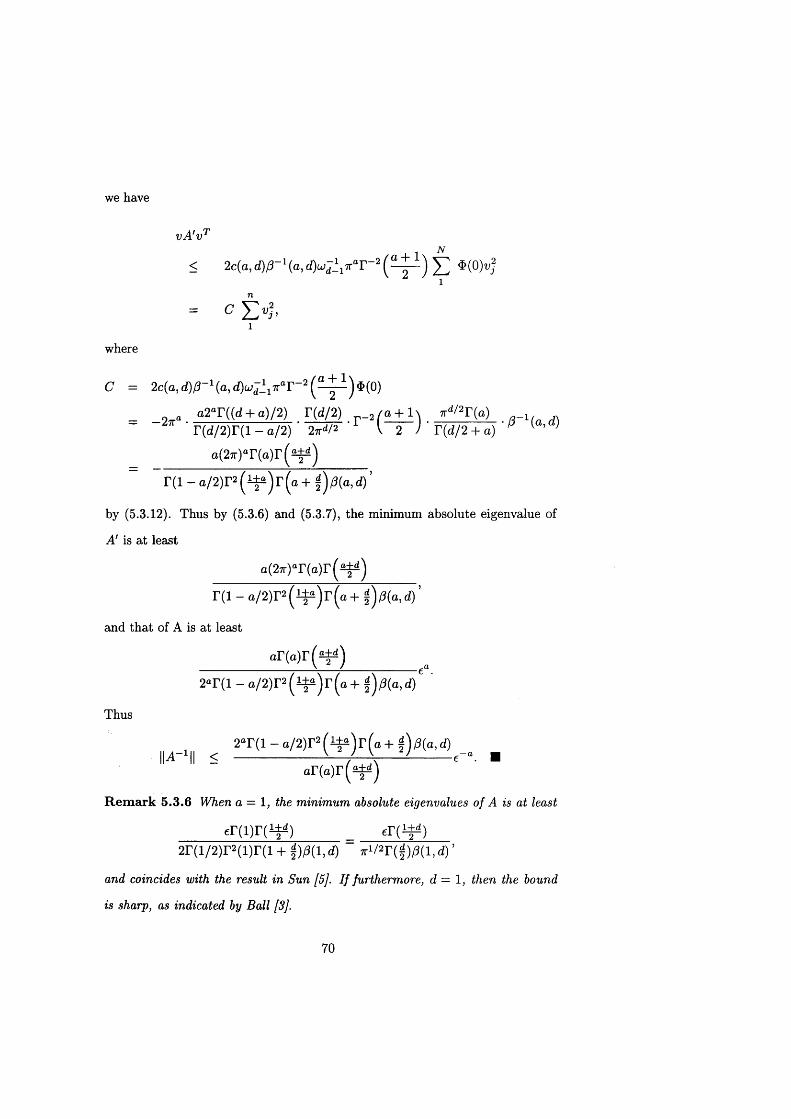
we have

vA 'vTN

< 2c(a ,d )0-1{ a ,d ) u ^ 1n ‘ r - 2( ^ - ) j 2 *(<»«*

= C ± v } ,1

where

C = 2c(a,d)/)-1(a,d)w^ l)r“r - 2( ^ ) $ ( 0 )

a2°r((rf + q)/2) T(d/2) r - , / ’a + l'> *d' 2T(a) ,r(d/2)r(l - o/2) 2 ^ /2 I 2 / T(d/2 + a) ’ '

= - 2 tt

a (2 T )« r(a )r (s ± i)

r ( l - a /2)r2 ( l± s ) r (a + f ) 0 (a, d) ’

by (5.3.12). Thus by (5.3.6) and (5.3.7), the minimum absolute eigenvalue of

A 1 is at least

q ( 2 7 r ) T ( a ) r ( ^ )

r ( l - a / 2 ) r 2( l f i ) r ( a + f ) /3(a,d)’

and that of A is at least

ar(o)r(a± i)

2 T (1 - a / 2 ) r 2 ( i± 2 ) r ( a + f) /J (a ,d )e .

Thus

||A->|| < 2°r ^ ~ a / 2)r ^ ( l ^ ) r (a + g )^ (a ,d )

oT(o)r(2±i)

R em ark 5.3.6 When a = 1, the minimum absolute eigenvalues of A is at least

eT(l)r(±±4) _ eT(i±^)

2r(i/2)r2(i)r(i + f)/3(i,d) “ * w r { % ) 0 ( i ,d ) '

and coincides with the result in Sun [5]. I f furthermore, <2=1, then the bound

is sharp, as indicated by Ball [3].

70

R em ark 5.3.7 In [48], the upper bounds are given for the spectral norm of

inverse of the interpolation matrices for all the functions which are strictly con

ditionally positive definite of order 0 or 1. But the estimate is not as accurate

as ours in this case. In fact, from [48], we get

11*11“ = r (1 ~ rc-MWD) „ * fip(u) dUtJo

where p(u) = —c(a, d) u~a~d.

Thus according to Theorem 3.5 of [48], we get

IIA-1II <'ydp(2'y/q) ’

where

q = e/2, 7 = 12[~r2 (-(- ' + 1^ 2) ]V(d+i)y

Hence by computation, we get some data on the norm of the inverse of A as a

table below.

a, d, our estimation, [48]’s estimation

1.1, 3.507c-1-1, 89?r0-5 c "1-11.1, 11, 10.075c"1-1, 0.245 x 107 tt0 09 c " 111.1, 91, 31.314c"11, 0.73 x 1032 tt0 0^ " 111.1, 108, 65548.7 e "11, 0.248 x lO30103004 e~1A

1.4, 1, 5.612c"1-4, 256tt0-7 e "1-41.4, 11, 18.9c"14, 0.738 x 1077t°-117 e " 1-41.4, 91, 78.2c"1-4, 0.29 x 10337t0 015 e " 1-41.4, 108, 1313058.9 e "1-4, 0.814 x io 30103005 e " 1 4

1.75, 5 15.87 e "1-75, 1057.7 7rO-875e-1.751.75, 11, 58.088 e "1-75, 0.18 x 87r0159e"1-751.75, 91, 356.98 e "1-75, 0.25 x 1034 t t 0 019 c " 1-75

1.75, 108, 62124744.5 e"1-75, 0 741 x io 39193997 e " 1-75

71

5.4 Further remarks

We do not proceed to estimate the upper bound for the norm of the inverse

of the interpolation matrix associated with the Hermite radial basis function

interpolation in R d. We refer the interested readers to Narcowich and W ard’s

paper [49], where such results axe obtained for some special cases of Hermite

interpolations. The mechanism is virtually the same as the one in the case of

radial basis function Lagrange interpolation.

In [54], Schaback obtained the lower bound for the norm of the inverse of

a radial basis function interpolation matrix through best approximation theory

approach. This approach can be applied to get the lower bound for the norm of

the inverse of a radial basis function Hermite interpolation m atrix with minor

modification. However, we will leave this technique to be used in the case of

interpolation on the sphere in the next Chapter.

72

Chapter 6

Stability of interpolation ong d - 1

6.1 Introduction

Like its counterpart in ]R,d, the Hermite interpolation on S d~l by radial basis

function leads to the following system

f E£Li a i[L i> Lj * h] + £z=i PiiL k, Pi] = yjfe, 1 < k < N, (6 ID \ Ei=i Pj] +0 = 0, 1 < j < Q.

Here h : [— 1, 1] »-> ]R is a suitable smooth function, n m(5d_1) the subspace

of spherical polynomials of degree less than m, A = { L i , . . . , L ^ } c E'r the

interpolation distribution set, j/i, . . . , j/ jv G S d~l the interpolation data values,

and pi, . . . , pq a basis of n m(5d_1), with Q = d im n m(5 d_1). In m atrix form

the system (6.1.1) reads as

u { l ) = (p PoT) 0 ) = ( o ) ’ f6-1-2)with

A = ([Ij,!,./*])"

The sensitivity of the interpolation system is determined by the condition num

ber of the matrices A and U, which is the main topic of this chapter. First we

introduce some preliminary lemmas.

73

6.2 Preliminaries and lemmas

For 0 < S < 1 and integer k > 1, let

( t - S ) k6 < t < 1,

/«,*(*) = s ( i -<&)*’0, - 1 < t < 6 ,

which is continuous when k > 1, and has the Gegenbauer expansion of the form

OO

n = 0

For n > k, by integrating by parts k times, refering to (2.2.23), have

}s,k(n) = J js,k(t)PiX,m ~ i2)A“ 1/2d(

= An,A J i / J,t(«)i?’,( ( l - t 2)"+A- 1/2)dt

= An,A( - l ) ‘ J f $ ( t ) D " ~ k(( 1 - «2)"+A- 1',2)di

= A n ,A * ^ ~ ^ * / ' P n - ‘ ( (1 - i 2 ) ( » - ‘ ) + ( * + ^ ) - l / 2 ) d j

= j \ h n - k,X+k ) - l P m m i ~ t ^ - ^ d t

_ & ! ( - ! ) * / in A Z 1 p t+ A i- tW l _ ( 2 > t + A - l / 2 , , (

(1 - S)‘ A„_M + * / , » -* U (

If we set a (n ,k ,X ) = (-l)* /i„ ,A //in-*>A+*» then

_ f (n + A)r(n + l)r (n + 2A) 1 1/2 ( - 1)”">A \ 22A“ 1(r(n + A + 1/2))2 J 2nn! '

Therefore

a(n, A:, A)

= ( — 1) hrijX/hn—kyX+k

f (n + A)r(n + l)r (n + 2A) ] 1/2 ( - l ) n 2n~*(n - A;)!\ 22A_1(r(n + A + 1/2))2 J 2»n! ( - 1 ) ”-*

22(A+fc)_1 (r((n - k) + (A + fc) + 1/2))2 1 1/2X 1 ((n - A:) + (A + A:))r((n - A;) + l ) r ( (n - A;) + 2(A + k)) J

74

f r(n + l)r (n + 2A)22fc \ 1/2 ( ~ l ) k(n - k)\\ T(n + 1 - k)T(n + 2X + k) ) 2kn\

f n\ T(n + d — 2) | 1/2 ( ~ l ) k(n - k)\t(n-fc)! r(n + k + (d — 2)) j n\

(_!)* \ { r i - k ) \ ( n + d - 3)! | 1/2n! (n + (d — 3) + k)\

where in the penultimate equation we have used A = (d — 2)/2. Now

^ p ’ = 1 /{(n (n - l ) " - ( n — k + 1)} n!

< ( n - k + l )~ k .

If n > 2k, then (n - k + l ) _fc < (n/2)~k = 2kn ~ k; if k < n < 2k, then

(n — /c + l ) -fc < 1 < (2k)kn~k. Meanwhile,

(n + d 3). _ 2/{((n + d — 3 + k) • • • (n + d — 2)}(n + d — 3 + k)\

< (n + d — 2)~k < n~ k,

as d > 2. It follows that

\a(n k A)| = f (w ~ *)! (n + d ~ 3)! \ 1/2|a ( n ,«, A)| | n , (n + ( d _ 3) + jfc)i J

< (2k)kn~k,

for n > k.

Meanwhile, by Cauchy-Schwarz Inequality, we have

1 / P k± £ ( t ) ( l - t 2)k+x~1/2dt 1 Js

( r1 \ 1 / r 1 N1//2< [ J (Pk± l( t ) )2( \ - t 2)k+x- l /2d t \ ( j ( l - t 2)*+A_1/2^

Q f (1 - t 2)k+x~1/2dt^j<

< C (1 - £)(fc+A+1/2)/2.

Here C > 0 denotes an intrinsic constant independent of 5 and n, not necessarily

the same at each occurence. Hence, for n > k, we have

< ( 1 _ ^ „ t ( l - * ) (A+W2)/2

75

Now for 0 < n < k, we have

lA.*(n>l = m i - e r ^ d tJ JR

f d(pLx)m 2(i - «2)A“1/2d t1/2 [ J(/wt(‘))2( i - * v ~ 1/2<«R, */]R

< C ( l - S ) ^ +1 \

Thus we have

L em m a 6.2.1 The function fs,k for k > 1 is continuous on [-1,1], has support

on [5,1] and has the following Gegenbauer expansion

OOh,k =

n = 0

1 / 2

where the Fourier coefficients fs,k(n) satisfy

C (1 — <S)(A+1/2)/2, for 0 < n < /c,\fs,k(n )\ < | Cn fc(l — 5)(a+1/2 *)/2, f o r n > k .

with some constant C > 0 depending on k and A only.

(6.2.3)

Now let

As,k = fs,k * fs,k-

Then, we have

L em m a 6.2.2 The function A$,k is o, (2 k-2 )- t im es continuously differentiable

function on S d~l and has the following form of absolutely convergent Gegen

bauer expansion

As ,k = As!k{n)P^x\ (6.2.4)n = 0

76

where the Fourier coefficients

A 5,k{n) = P(n, d)f$ k > 0

for n > 0. Furthermore,

A (n \ k ,

for some constant C > 0 depending on k and A only. Here

/3{n,d) = ^ = C?(n-(d- 2)/2)un ' '

is from (2.2.25).

P roof

The assertion on the Fourier coefficients Ag,k(n) follows from Lemma 6.2.1 and

Theorem 2.2.8. Hence for fixed 5 > 0,

A i<k(n) = o(/3(n,d) n " 2‘ ) = o ( n - “ -<d- 2>/2) .

Thus by Corollary 2.2.13, A$,k is (2k — 2)-times continuously differentiable. ■

L em m a 6.2.3 The function A^,k has support { t : 252 — 1 < t < 1}, and satisfies

^ ,* (1 ) > S(fc,d)(l -

where

B (k ,d ) = 1(2k + l)22fc+A+1/ 2

P roof

By [25, Lemma 2.3], As,k(t) ^ 0 if and only if

cos(2cos-1 5) < t < 1.

77

Since cos(2 cos-1 <5) = 2cos2(cos-1 <5) — 1 = 262 — 1, it follows th a t A$,k has

support { t : 2S2 — 1 < t < 1}.

Next, noting that x 2 = 1 for every x e 5 d_1, we have

A Syk{ 1) = A s,k(xx)

= —~ - f f l k ( x z ) d zSd-2 J s d~1

~ / ( x z - 6 ) 2kdz0) Z k S d - . 2 J x z > 6

>

>

>

' ---- [ ( t ~ 6 ) 2k( l - t 2)x 1/2dt f dwd- 2{y)- 0 ) S d —2 J s J s d~2Q ^ ./(J

r ((5+ l) /21 /*!

- ( ( S + l ) 2/ ^ - 1/ 2 /•(<5+1)/2/(1 - 5)2* Js (* V 2 dt

1 - (<5 + 1)/2)a~1/ 2((<5 + l ) / 2 - <5)2fc+1(2* + 1)(1 - <5)2fc

(1 - (5)A+1/2

(6.2.5)

(2& + i)22fc+A+1/2 *


Let

C ( 0 )= [ y^dy, 0 e N t 2-J S d~ 2

Then the constant C{2(3) > 0.

L em m a 6.2.4 For {3 = ( f t , . . . , j3d) 6 and 0 < 6 < 1, /e<

7^(5) = f 1 t ^ { t - 8 ) 2k- ^ { l - t 2)x- l / 2dt.J (5

Then there exist positive constants C\ , C2 independent of 5 such that

C2( 1 - 5 )2*-I/jI+ a + 1/ 2 < 7^ ) < _ ^^2fc-|/3|+A+i/2 ( 6 2 .7 )

(6 .2 .6)

78

P ro o f

It is obvious that

Ip (8) = f 1 t ^ ( t - 8)2k~ 1 1(1 - t 2)x- ^ 2dtJ s

< f 1 {I - S)2k~W {l - 62)x~1/2dt J 6

< C i( l - S)2k~W+x+1/2,

with constant C\ = 2A-1/ 2. Conversely,

1/3(8) = J ^ ( t - S f b - W i l - t ^ - ^ d t

> / t?1( t - S ) 2k- W ( l - 1 ? ) x- 1/2dtJs

r(8+l)/2> S ^ i l - d S + l ) ^ ) 2) ^ 1/ 2 / ( t - 8 ) 2k~W dt

> C2( l - 5 ) 2fc_l/?l+A+1/2,

where

C2 = 8?1 (3 + 8)x- 1/2/2 2X+2k+2~\P\ > 0. ■

We note from (2.2.13) th a t every distribution of order r supported a t one point

x e S d~ 1 can be expressed in the form

L = L i + L 2 = Y , C0 S * o D ( 3 + Y . c 0 S * ° D **' ( 6 ' 2 -8 )

I P \ = r \0 \ < r

L em m a 6.2.5 Let x be a fixed point on 5 d_1 and let L be defined by (6.2.8),

with r < k, and that neither L nor L \ annihilates the spherical polynomials

space n ( 5 d _ 1 ) . Then there exists a constant C > 0 independent of 8 such that

J := [L, L * Astk] > C (1 - 5)-2r+(d-i)/2 (6.2.9)

P ro o f

Since A$,k is a (2k — 2)-times continuously differentiable function on the sphere

79

and r < k , the expression J is meaningful and

J = l L , L * A d,k] = l xL» [ f s,k(x z ) f s,k(yz)dzJs*-1

= f [L(f iA(z)]2<iz >0

as L does not annihilate the spherical polynomials space H (Sd~1). It follows

that

7 = ^ - ^ 2kl J ^ w ^ W Axz~5)kjrWli dz= (1 — 6)~2k apa7 f z 1+P(xz — 8)2k~ ^ +^ d z ,

\P \,h\<r Jxz>6

where ap = (cpk \/(k — |/3|)!^. To estimate

[ z ^ + 0 { x z - S ) f ~ l0 + y l d z ,J x z >6

note th a t the sphere is symmetric, and without loss of generality, assume x =

(1, 0, . . . , 0). Letting t — x z = z \ , we then have for every \fi\ < 2k,

f z@(xz — S)2k~ ^ d z .J x z > 5

= [ y0'd S d~2(y) f 1 t?l (t - S)2k~W(1 - t 2)x~ ^ 2dtJ s d- 2 Js

= c m i m ,

where ($' = (fo, ■ • • > fid) € INo-1 , and C(fi')i Ip{$) 31,6 defined as in (6.2.5) and

Lemma 6.2.4. Hence

J = (1 Y , apaiC(/}' + 7' ) b +-,(S).\P\> |7 |< ’"

By Lemma 6.2.4,

I p + y ( S ) = C ( 1 - <5 )2 * - |/3 + 7 |+ ( d - l) /2 )

for some positive constant C. If |/3| = |7 | = r, then

/ / j + 7 (<5) = C ( 1 - S ) 2 * - 2 r+ (d - l ) /2 _

80

If, say \{3\ < r, then for every index 7 , |7 | < r,

I 0 + 7 (S ) = C(1 - ^ - l / J + T l + f d - 1) / 2

> C(1 -<5)2*~2r+(d-1)/2.

It follows that, when S < 1 is sufficiently near 1, the only contributions that

makes

I/J+7(<$) > C( 1 - 5 )2* - 2r+ (d -l ) /2

for some constant C > 0 is from L \. Since J > 0 and L \ does not annihilates

II(5 d-1), we have

J > C ( l - « 5 ) - 2r+(d- 1)/2,

for some constant C > 0. ■

6.3 Upper bound for ||j4_1||: The r-SPD and r- SCPDi cases

6.3.1 Lagrange interpolation

In this section, we will estim ate the upper bound of ||A_1||, the spectral norm

of the inverse of the interpolation matrix A, where A = (A i j ) with entries

Aij = h(xiXj). Here the function h is either a SPD function of the form

OO

h = y : h(n)Pj^ , h{n) > 0 for n > 0, (6.3.10)7 1 = 0

or a SCPDi function of the form

OO

h = ^ h (n )p (x\ h(n) > 0 for n > 1 (6.3.11)7 1 = 0

satisfying h( 1) < 0.

81

L em m a 6.3 .1 [3, Lemma 2] Let h be defined by (6.3.11) satisfying h( 1) < 0.

I f for some constant 0 > 0,

N N N

^ CiCjAij > whenever = 0,i,j=1 i=l i=l

then all the eigenvalues of A have absolute values of at least 9.

T h eorem 6 .3 .2 Let

OO

h = h (n )p (x\ h(n ) > 0 for n > m , (6.3.12)n = 0

be absolutely convergent. Suppose for some natural number k > 0 and some

constant C > 0,

-r, s J C fi(n, d)n~2k, for n > m a x{k ,m }— ( C (3(n, d), for m < n < max{A;, m ).

holds. Then, for any N distinct points x^, . . . , £/v € 5 d_1 with r) = min{/9(xj, Xj) |i ^

j }, there exists a

0 > C rj2k

such that

N N2 CiCjh(xiXj) > i,j=1 i= 1

whenever YliLi ci&xi annihilates n m(5d_1). Here C > 0 is an intrinsic constant

independent of N and rj, not necessarily the same at each occurrence.

P ro o f

Let 5 = max{xiXj | i ^ j } . Since xy = cosp(x, y) for x , y e S d_1, noting that

0 < rj, 6 < 1, we have 6 = cos rj. Hence we have the following relation between

6 and 77,

( 2 / t t V < 1 - 6 <r)2. (6.3.13)

82

2> 0,

Let 0 7 c = (ci, . . . , c n ) G IR, such that J2iLi c*^. annihilates IIm(5 d-1). By

the Addition Theorem 2.2.26,

TV TV dn

£ CiCjP<XH*<Xj) = £ CiCjf3{d, n) 5 YUyi (#t)T n,f (^ j)*,i=i i,j=l z=i

dn tv

= 0 (d, n) £ | £ c ^ w |z=i i=l

as P(d, n) > 0. Set K = max{m, A;} and £i = \ / (2 + <5)/3. Then by Lemma 6.2.1,

noting th a t Y liL i c^ x i annihilates n m(5 d_1), we have

TV TV oo

^ v CiCjhfaiXj) — ^ C i C j ^ h ^ P i ^(xiXj)i,j=1 i, J=1 n = 0

oo TV

= 5Zh(n) 53 CiCjP(x ) {xiXj )n —0 i , j = l

oo TV

= 53 53 CiCi PnX)(XiXj)n —m i,j= 1

A T -l oo TV

" 21 £ C C j - P f W ,)n = m n=/C

K - 1 AT> [<7 ( 1 - < 5i ) (A+1/2) 5 3 Ajlf*(n)] a c j P W f a x j )

n = m i , j = 1

oo TV

[<7 ( 1 - < 5i ) * ~ (a+ 1 /2 ) 5 3 A i ,* (« ) ] C jC j-P ^^X iiC j-)

n = m i , j = 1

oo TV

+ r “ ' \ ; ,_n = K i, j —1

oo TV

> C ( 1 - ^ ) ‘- <A+1/2) £ A Suk(n) £ CiCjP^HxiXi)n = m i , j = l

oo TV

= <7 (1 - 5 3 Agi,k(n) 5 3 CiCjP^^iajj)n = 0 i, j = l

TV

= <7 (1 - <Si)*_(A+1/2) 5 3 i, i= i

In the last inequality we have used the fact th a t (1 — Si)k < 1. Note that

Supp A suk = {t | 26l - 1 < t < 1},

83

and since

28\ - 1 = 2(2 + 8)/3 - 1 = (28 + l ) /3 > (28 + 8)/3 = 8,

we have

AT IV

CiCjhixiXj) > C ( l - 8 i ) k- ^ +1/2)^ 2 ( ^ A s u k(xiXi)i , j = 1 i = l

2 — 1

> C (1 - <51)*-(A+1/ 2>(1 _ <51)(^+i/2) ^ c2

k N

> c V c 2W f cJV

t = l

by Lemma 6.2.3 and the fact that

i - ^ t - v w r m = > (1 ~ *>'*■

Noting th a t (1 — <5) > (2 /n 2)rj2, we therefore have

N N

^ 2 CiCjh(xiXj) > Cri2kY 2 ch i , j = l i = 1

for all 0 ^ c = (c i, . . . , c n ) £ IR^ such th a t YliLi annihilates n m(Sd_1]


As a result of Theorem 6.3.2, we have

T h e o re m 6 .3 .3 Let h be as in (6.3.10). Suppose for some natural number

k > 0 and some constant C > 0,

holds. Then, for any N distinct points X\, X2 , • . . , x n £ 5 d_1 with minimal

separation distance 0 < 77 = min{p(a;i, Xj) | X{ ^ Xj}, the interpolation matrix

A = (h (x iX j)) is such that

P _1|| < C r ,- 2k,

for some C > 0 independent of N and 77.

P ro o f

By Theorem 6.3.2,

N N

CiCjh(xiXj) > Cr}2h Y 2 cii, j=1 i= 1

holds for all 0 ^ c = (ci, . . . , c^v) E 1RN , which implies th a t the eigenvalues of

A has absolute values of a t least Cr}2k by the Courant-Fischer Theorem. Hence

the spectral norm of the inverse of A satisfies

P - 1 || < C r )~ 2k. ■

T heorem 6 .3 .4 Let h be as in (6.3.11) satisfying h( 1) < 0. Suppose, for some

natural number k > Q and some constant C > 0, the inequality

C /3(n,d)n~2k, for n > k,h{n) > C 0 (n ,d ), for 1 < n < k,

holds. Then, for any N distinct points x \ , x?, . . . , x n £ S'd _ 1 with 77 = min{p(:ri, X j ) |i 7

j } , the interpolation m atrix A = (h(x{Xj)) is such that

I I^"1I I < c , t7-2*,

for some C > 0 independent of N and rj.

P ro o f

By Theorem 6.3.2,

N N

CiCjh(xiXj) > Cr)2k Y 2 cii , j = 1 i = l

85

holds for all 0 7 c = (ci, . . . , c n ) G such that YliL i c* = 0- Thus by

Lemma 6.3.1 and the Courant-Fischer Theorem,

R e m a rk 6 .3 .5 In [46, (2.78), (3.20)], Narcowich, Sivakumar and Ward estim

ated that, under the same assumptions for h,

which is as big as the square of the estimates obtained in Theorem 6.3.3 and

Theorem 6.3.4-

6.3.2 Herm ite interpolation

Now we can similarly estim ate the upper bound for spectral norm of inverse of

radial basis function Hermite interpolation m atrix based on the r-SPD function

h, using Lemma 6.2.5. For simplicity, we just prove the case when h is r-SPD.

Recall from (2.2.18) th a t every distribution on S d~1 pointwise supported at

xq € S d~1 can be expressed in a form

T h e o re m 6 .3 .6 Let h be defined by (6.3.10)., Suppose for some k G IN and

some constant C > 0, the inequality

holds. Then, for any set of M distributions {Li = 5Xi o pi(D ), 2 = 1 , . . . , M }

with distinct supporting points x \ , X2 , • • •, xm G 5 d_1 and

P - 1 || < C r ] -2k. m

\\A x|| = 0 (r ) 2 log rj x) 2fc

where p is a m ultivariate polynomial in JRd and

D = (d /d x i , . . . , d /d xd ).

C /3(n,d)n 2k, for n > k,C P(n, d), for 0 < n < k.

a m ax{ai = degpi | i = 1 , . . . , M } < r,

min{o!i = degpi \ i = 1, . . . , M},

(6.3.14)

a (6.3.15)

86

M

= C (1 - c?[£i, Li * A Suk]i= 1

M

> C ( 1 - ^ i)A:_(d_1)/2C,i [ 5 Z ci ( l - (5i)(d“ 1)/2" 2ait=lM

> C (1 - t f i )* -^ -1)/2*?! [ X ) c ? ( i - <51)(d-l)/2-2ai=l

M

> c ( i - i ) ‘- 22 [ £ c ? ] ,i=l

by Lemma 6.2.5. Hence, by (6.3.13),

M M

^ 2 cic3 iL i , L j* h ] > C n2k~AgL [ ^ 2 c?] •i, j = 1 i=l

Since this inequality holds for arbitrary nonzero vector c G lNd, the conclusion

of the theorem follows. ■

6.4 Lower bound for \\U- l

Having obtained the upper bound for norms of inverses of interpolation matrices

for the cases when h are r-SPD and r-SP D i, we now turn to a lower bound

for the spectral norm of the inverse of the interpolation m atrix U when U is

invertible. This time the basis function can be any r-SC PD m function. Recall

th a t the radial basis function Hermite interpolation can be expressed in the

m atrix form as: given y = (yi, . . . , yw) G IR^ and distributions {Li = 6Xi o

Pi{D), i = 1, . . . , N } with distinct supporting points x i, X2 , . . . , x m € 5 d_1,

find c = (ci, . . . , cn )t G IR^ and (3 = ((31 , . . . , /3V)T , where u = d im n m(5 d_1),

such th a t

where

t t ( (-^i) L j * h) (L i , q~f)~ ' (L j, <?7) 0

with 1 < i, j < N and 1 < 7 < v.

Note th a t when h is r-SC PD m and the set A = {Li, . . . , L n } is IIm(5 d_1)-

admissible, U is always invertible, which is the asumption from now on.

For h G C[—1, 1], define

E n (h) = min max \h — p\. peni |t|<i

It is well-known, see [40], th a t if h G C 2 t[— 1, 1] then

E n { h ) < C n ~ 2T,

and

E n (h^a)) < C n ~ 2T+a, for a < 2r.

We will follow the approach of Schaback’s best approximation technique [54] to

get the lower bound on | | t 7 —1 1|. To begin with, let || • ||r and || • ||s be the l r and

l s vector norms on ]R/v+l'. The norm || • H2 is the usual Euclidean norm || • ||.

Define the m atrix norm

||B ||r ,» := sup { ||B x ||r / | |x | |s | x € R w+7 { 0 } } .

Obviously for every N x N m atrix B ,

Halloo,1 = , max \Bij\,l < t , j < N

and the spectral norm

N

ll^ll = l|B||2,2 = < AT IIJ5IU.13= 1

For every p G IIn (]R), define a m atrix

Up = ( ) , with l < i , i < N , l < ' y < v , (6.4.17)

89

and a subspace

{ N N ' j

5 ~2ciL i*p + q q ^ 2 a L i e S'm>T> (6.4.18)

i= 1 i= 1 Jof the space n „ ( 5 d-1). When n is sufficiently large, we can choose p G n n (lll)

which is close enough to h on [-1,1] such that

\ \U - U p\\,tr ■ | | ^ _1||r,S < 1. (6.4.19)

This inequality ensures th a t Up is invertible too; see [54]. Let

p(n) := max dim n p. (6.4.20)P€ n„(]R)

Note th a t u < p(n) < N + v. Let

n* := max {n > 0 | p(n) < N } . (6.4.21)

Then //(n*) < N and hence for every p € IIn, (R ), the polynomials {L \ *

p , . . . , L n *p } axe linearly dependent functions, which implies th a t Up is singular,

and hence the inequality (6.4.19) is violated, i.e.,

I |t/_1|lr,s > \ \U - U p\\: l , V p € n n. ( R) . (6.4.22)

This relates a lower bound for ||£/-1 ||r,s to the matrix-valued approximation

problem of U by Up. The entries of the error m atrix U — Up are zero except for

the sub-main-matrix A — A p with entries

[Li, L j * h ] - [Li, L j * p ] = L ^L jh (xy ) - L ?L jp(xy),

for 1 < i, j < N . By Jackson’s theorem,

\ m ) h ( x y ) - m ] p ( x y ) \ < C E n. ( h {m))

< C n 7 <2T- 2s),

as h e C 2 t[— 1, 1], where a = maxi<i<;v{ci;i = degp*}, the highest order of

distibutions Li, i = 1, . . . , N . In conclusion, we have

90

Lem m a 6.4 .1 The inverse o f the interpolation matrix U satisfies

l l ^ l l i . o o > C n lr- 2S,

||£/_1|| > C n lT~2“/N .

It remains to determine the integer n*. From its definition, we have

/i(n*) = m ax dim lip < dim n n„(Sd-1),Pe n n.(]R)

hence

/a(n*) < dim IIn, ( 5 d_1) < /z(n* + 1 ). (6.4.23)

By Equation (6.4.21),

//(n*) < N < /z(n* + 1). (6.4.24)

These two inequalities show th a t dim IIn, (<S'd_1) = O ( N ) . Now since

dim n n, ( 5 d" 1) = 0 ( n f - 1) ,

we have

n* = C>(lV1/<d- 1>).

Combining with Lemma 6.4.1 we have

T h e o re m 6 .4 .2 There exists a constant C independent of N such that the

inverse of the interpolation m atrix U satisfies

\ \U -1\ \ > C N ( 2T- 2S>Kd- 1)- 1. (6.4.25)

Let us point out the relationships of N with the minimal separation distance

ri = min{d(xi, x j) | i ± j } , in order to compare the lower bound here with the

upper bounds in Section 3. Since all the interpolating points are on 5 d_1, it is

easy to deduce th a t

r) < l/A^1/(d_1).

91

If the points are regularly distributed on the sphere, then

rj > O O .

Thus we have

T h e o re m 6 .4 .3 Let the support of the interpolating distributions {L \, . . . , Ljy}

be pointwise supported and the supporting points be regularly distributed on S d~1.

Then the interpolation matrix U satisfies

WU-'W > C ^ - 2r+2“+(d“ 1)j (6.4.26)

where C is a constant independent of N or 77.

6.5 Further remarks

From the upper and lower bounds for the spectral norm of the inverses of the

interpolation m atrices A and U, respectively, we see th a t the smoother the basis

function h, the more sensitive the interpolation matrices become to the minimal

separation distance 77, a t least when the interpolation points are regularly dis

tributed. Meanwhile, from the work of [24, 15, 32, 12] and the convergence

rate result in Chapter 8 and Chapter 9, we know th a t the smoother the basis

function h, the higher the convergence rate of the interpolating approximation.

It seems th a t there is a trade-off between the stability of interpolation and the

convergence ra te of approximation, which is reminiscent of the so-called Uncer

tainty Principle in quantum mechanics, and is discussed in detail by Schaback

[53] in the case of radial basis function interpolation in R d.

92

Chapter 7

The variational theory

7.1 Introduction

The classical variational approach is discussed in detail by Duchon [10] for

interpolation beginning with a semi-norm (the energy norm) || • ||m. For a given

set of interpolation d a ta {(xi ,yi ) € xlEt : i = 1, . . . , N } , one seeks s in a

suitable space X such th a t s(x{) = yi, i = 1, . . . , N and

I ML = min { 11 /! I m. | f {x i ) =y i , i = 1, N and / G X j.

This technique has been used widely and fruitful results are obtained, among

them are Duchon [10], Meinguet [39], and Powell [51]. It has the advantage of

deriving the error bounds of the interpolation with ease. Golomb and Wein

berger [18] and Light and Wayne [27] have used the representer theory to get

the error estim ate for interpolation, with a heavy flavour of variational theory

underneath.

In [37, 38] Madych and Nelson have described another variational approach

for interpolation using conditionally positive definite functions. Unlike Duchon’s

approach, they begin with a continuously conditionally positive definite function

h and construct a admissible space Ch based on h. Then using the reprodu

93

cing kernel H ilbert space theory they establish pointwise error estimates as the

interpolation points become dense. We point out th a t Wu and Schaback [65]

using the Kriging m ethod have also obtained such results.

In this chapter, we are going to follow Madych and Nelson’s variational ap

proach to prove th a t the radial basis function Hermite interpolant is the optimal

interpolant with respect to a certain semi-norm || • \\h determined by the basis

function h. Through this technique, we will deduce the error bounds for the

Hermite interpolation in space R d and on the sphere. Moreover the admissible

space Ch determ ined by the basis function h will be fully characterized. This

approach is presented in its general form, so th a t the text will be adaptable to

include not only the cases of the space and the sphere 5 d_1, but also other

cases, e.g. manifolds, homogeneous spaces and compact groups.

Let G denote a domain in ]Rd and C(G) (respectively C 2r(G)) the set of

continuous (respectively 2r-tim es differentiable) real valued functions on the

domain G. Let £'T be the dual space of C T(G)), composed of distributions of

order a t most r . Let h € C 2 t(G x G). Let n m denote the set of polynomials of

degree less than m o n G . Let £'m T be the subset of S'T whose elements annihilate

n m. For L e S'T and / € C T{G), the operation of distribution L on / is defined

by

[L, f }

and the convolution

L * h (x) = [L, h{-, x)].

D e fin itio n 7 .1 .1 Let the set of distributions A = {Li , . . . , Ljy} C S'T. The

radial basis function Hermite interpolant to f G C T(G) is a function of the

94

form

N

*(*) : = ^ c fL i * h ( x ) + p ( x ) , p e n m , (7 .1 .1 )

where J2iLi ci^ i £ subject to the interpolation conditions

[.L ,s] = [ L , f ], L e A.

W ith reference to the above definition, A is IIm-admissible if A(p) = 0 for

all p € n TO implies p = 0. Note also th a t we recover the usual interpolation

problem if all of the elements of A are point evaluation functionals.

D e fin itio n 7 .1 .2 A function h : G x G R is called T-CPDm on G if, for

every positive integer N and every set of distributions A = {Li , . . . , L ^ } C S'T

on G, the inequality

N

^ 2 CiCj[Li, L * h] > 0 (7.1.2)iyj— 1

holds whenever c = (ci, . . . , c n ) satisfies

N

T cAL ii P] = f or P e n m-i = l

I f the above inequality (7.1.2) is strict whenever 0 ^ 0 YliL i ci^ i annihilates

Um , then h is called T-SCPDm .

It is easy to check by the proof of Assertion 1.1.3 th a t the radial basis func

tion Hermite interpolation defined above is uniquely solvable whenever h is

r-SC PD m and the distribution set A is n m-admissible, which are the assump

tions throughout this chapter. F irst we characterize the admissible semi-Hilbert

space related with the r-SC PD m function h on G.

95

7.2 The admissible space

For every pair of distributions L i , L 2 € S'm T, we define

( L \ L 2 ) = [ L i , L2 * h].

Since h is r-SC P D m, by Definition 7.1.2, [L, L*h] > 0 whenever 0 / i G £m,r-

Hence (•, •) is an inner product on £'m T. Let H be the closure of £'m , th a t is,

H = {L | (L,L)V2 < 0 0 }. (7.2.3)

The set H is the Hilbert space with the norm inherited from the inner-product

on S'm T. Define the map $ on H by

$ (L ) = L * h , L e H .

Then 3>(L) = 0 if and only if L = 0. For if $ ( L ) = 0, then

0 = [L, *(L)] = { L , L * h ] = (L, L )h ,

which means L = 0. Thus $ is a 1-1 mapping. Now set

c h = $ ( H ) ® n m.

L em m a 7 .2 .1 Let

( f l + P l , h + P 2 ) k := ( S - ' t f i ) , ■

Then (•, •)h is a sem i-inner product on Ch with kernel n m. We denote the

resulting semi-norm by || • ||/i.

P ro o f

T hat (•, -)h is a semi-inner product on Ch is clear from its definition. We need

only prove th a t its kernel is n m.

96

By the definition of (•, -)h, if p G IIm, then (p, p)h = 0. Conversely, if

/ € Ch, f & n m and ( / , f ) h = 0, then / = L * h for some L E H, and

( $ - ' ( / ) , * - ' ( / ) ) „ = 0.

Since $ is a 1-1 m apping and (•, - )#2 is a norm on H ,

0 = $ - 1( / ) = $ - 1(L * /i) = L.

Hence / = 0. This proves th a t IIm is the kernel of the semi-norm \\ -\\h- ®

T h e o re m 7 .2 .2 Let h E C 2r(G? x G) be T-SCPDm on G. The following state

ments are true:

(a) if L e then L * h + p E Ch for all p E n m;

(b) i f L E then

[L, f] = (L * h, f ) h for all f e Ch; (7.2.4)

(c) the kernel o f the semi-norm || • \\h is n m and Ch/H-m is a Hilbert space

with norm || • ||h/

(d) Ch C C T(G).

P ro o f

Statem ent (a) is obvious from the definition of Ch', (c) is justified by Lemma

7.2.1. It remains to prove (b) and (d).

Let L E S'm T, and let f € Ch- By the definition of Ch, there exists a 7 E H

such th a t / = 7 * h + p, where p E n m. Then we have

[L, f] = [L, j * h + p]

= [L, 7 * h\ = {L, 7 )H

— (L * h, 7 * h)h

= (L * h , f )h,

97

which proves (b). Now (d) follows from (b), because for every f £ Ch, [L, f] is

well-defined for all L £ Cm T. ■

R e m a rk 7 .2 .3 Part (b) of the above theorem is just the reproducing kernel

property. I t is more obvious if the distribution L is replaced by the point evalu

ation functional 5X. The representer for each L £ £'mT is L * h.

In the next theorem, we will make an equivalent definition of Ch which we

use to identify the Hilbert space Ch-

T h e o re m 7 .2 .4 A function f is in Ch if and only i f there exists a corresponding

constant c( f ) such that for every L £ £'m T , the inequality

P , /] | < c(f)\\L \\H (7.2.5)

holds. Furthermore, i f c*(f) is the infimum of all the constants c( f ) for which

(7.2.5) holds, then c* (/) = | | / | | fc.

P ro o f

If / £ Ch, then from (b) of Theorem 7.2.2, for every L £ £'m T ,

P . / ] I = I P * h, / ) * | < p * h | U | | / | U = P l l t f l l / I U .

Thus (7.2.5) holds with c ( f ) = H/H^ and hence c*(/) < \\f\\h-

Conversely, assume for a function / , (7.2.5) holds with c( f ) = c*(f) for every

L £ £!rritT ■ Define </>: £^l T i - > R b y

4>(L):=[L,f] , L e £ ' m,r .

Then <t> is a bounded linear functional on £'m T and is continuous. Since £'m T

is dense in H , 0 can be extended uniquely to a linear continuous functional on

H . By the Riesz representation theorem, there exists an unique element V £ H

such th a t

(£', L) „ = ^ ( i ) = [L, f] < c . ( / ) P | |« , VL 6 £U,T.

98

This inequality holds for all L € H as S'm T is dense in H . In particular,

Now by the definition of Ch, we can choose g = L' * h + p € Ch, so th a t

\\g\\h = \\L'\\h - By (b) of Theorem 7.2.2,

Because [L , / ] = [L, g] for all L e ^ T, we have / - j € IIm. Hence

/ = g + P € Ch and | | / | | fc = \\g\\h = \\L'\\H < c*(/), by (7.2.6). ■

Now let us see some concrete examples of Ch-

7.2.1 The case when G = lRd

Let the r-SC PD m function h 6 C 2r(lRd) have generalized Fourier transform h

on Q = ]Rd/{0}. Then by Theorem 3.3.2, for L € S'm>T,

Hence we have

T h e o re m 7 .2 .5 Let h be a T-SCPDm function on JRd and have generalized

{.L \ V ) h < c*(/)||L/||/f,

or I l l ' l lh < c * ( / ) . (7.2.6)

[L, g] = (L * h, g)h

= (L * h, L ' * h)h

= (L, L ')h = [L, f]

< c . ( / ) | |L ||h , VL e £'m T.

(7.2.7)

Fourier transform h on Q = JRd/ { 0}. Then the set

(7.2.8)

is the admissible space Ch-

99

P ro o f

First we prove th a t Sh C C T(R,d). Let / £ Sh • Then, for any L £ £'mT, we

the two integrals in the penultim ate equation being convergent as f e. Sh and

By Lemma 3.3.1, / £ C r (lRd).

Now select a test function rj £ V such th a t r/(0) = 1 and 0 < rf < 1. Set

Then rjs e V , 0 < fjs = < 1, and fjs —>• 7/(0) = 1 as 6 —> 0. By the

Approximation Theorem 2.1.6,

g = lim g *r)S,5-* 0

for every g £ C(lRd). For L £ £'m r and / £ Sh, let g = L * f . Then g is

continuous. Using the definition of the distributional Fourier transforms (2.1.6),

have

that L £ £'m>T C H . By (2.1.8), for L £ £'m T,

|£ | = o ( i e r ) asK I-x x ).

Hence,

^ > °)-

we have,

[L, f] = L * f { 0) = g( 0) = Jim s * r)5 (0)

100

= lim[L f , rjs]0—KJ

= lim[L, frfs]<5—>0

= i d L l m d

by the Lebesgue Dominated Convergence Theorem 2.1.4. Thus

\[L, /]l < c ( /) ||L ||h .

with1 /2

which implies th a t / G Ch-

Conversely, assume f € Ch- Then by the definition of Ch, there exists a

distribution L G H such th a t

f = L * h.

Then / = Lh. Note th a t \\L\\h < oo by the definition of H . Hence by Theorem

3.3.2, noting th a t h is non-negative,

oo > \\L\\2H = [ L , L * h ]

= [ \L\2hm d 1 1

■ i’r

- L m ~'-’TR

which implies th a t f £ Sh- This completes the proof.

R e m a rk 7 .2 .6 For the special case of Lagrange radial basis function interpola

tion, Theorem 7.2.5 was asserted by Wu and Schaback [65], but no explicit proof

was given.

7.2.2 The case when G = S d 1

Let h : [— 1, 1] ]R has the formal Gegenbauer expansion,

OO

A = ( d - 2 ) / 2 , (7.2.9)k=0

such that

hk = 0 ^ ( 1 + k)~2rP(k1d)~1^, with 2r > 2r + ( d — 1). (7.2.10)

Then by Theorem 2.2.10 and Corollary 2.2.13, for each fixed x G 5 d_1, h(x •) is

2r-times continuously differentiable on 5 d_1, and for all distributions L, T G S'T,

the convolution [L, T * h] is well-defined. If, furthermore, h k > 0 for k > m ,

then h is r-SC PD m on 5 d_1.

For every distribution L G S'T, by Theorem 2.2.10, the convolution

oo d*. ___L * h = Y ^ ^ P ( k ’d)hkLk,jYk,j,

k=0 j=1

and the operation

oo dfc

k=0 j=1

for every / G C T(5 d_1) with the expansion

oo dfc

/ = E E / * / w .fc=0 j= l

Furthermore, for L, T G £r ,

oo dfc _____

[ T . L . f t ] = ^ ^ 0 ( k , < r > h kf k J L k,j,k=0 3=1

and is well-defined. See Section 2.2 for details.

T h e o re m 7 .2 .7 Let

ak =0(k , d) h„. (7.2.11)

102

The setoo dk

Sh = { / | / = ^ ^ f k ' j Y k j and | | / | | fc < oo}, (7.2.12)k = 0 j = l

is the Hilbert space Ch, where for every f € Sh,

, 00 dh \ 1 /2

11/iu = { £ V E / I , } ■k = m j = 1

Here whenever ak = 0, its inverse aj"1 is interpreted as 0.

P ro o f

We first prove th a t if,

00 dh

/ = £ £ / ^ , ifc=o j = 1

satisfies

Jfe=0 ;/ '= l

then f € Ch- For any L G £ ^ r , we have

00 dfc

y! fk, jLk, jk=0 j =1

00 dfcy z h , j Lk ,k=m j =1

1/200 d*. \ f 00 dh

,A2 X I Z a * Z ^ * ’/lk—m j —1 ) \k=m j=1

1/2

Z ^ Z ^

Note th a too dh

\\L\\% = { L , L * h ] = ' £ a k J 2 \ L klj \ \k=m j =1

as L k j = 0 for k < m. Combining the last two equations we have

oo dh

| E £ f k j L kJ | < c{f)\\L\\H ,k=0 j = 1

with

I oo dh

° ( f ) = I Z ak 1 Z\ k=m j=l

1/2

103

Thus we haveoo dfc

= E E aAk = 0 j = 1

< c(f)\\L\\H, for all L € C |T. i7-2-1*)

and hence / € Ch-

Moreover, for every such f € Sh, we can construct an L f € H such that

I■£/(/) I — c(/)l l^/ l l i? holds. In fact, letoo dh____

5 3 a*: 5 3 f k’ k>jk=m j=1

be the formal expansion of L /. T hat is,

■k/jfcj “ a * for A; = m, m + 1, . . . ; j = 1, . . . , d*.

Then, since ajt is real,

(Af > Lf ) H = [Lf, L f * h]oo dh

= 5 3 a* £ i I '/ib>ji2k=m j~l

oo d fc

= E o 53i i2<o°’k=m j=1

so th a t L f £ H. Meanwhile,

oo dh

[ £ / . / ] = E E r / ^fc= m j = l

oo dfc

= 53a*53i i2-k=m j= 1

Therefore [L/, / ] = c(/)||-L /||ff. Thus c ( /) is the infimum of all the constants

such th a t the inequality (7.2.13) holds. Hence ||/ ||/i = c(/) .

Next we prove th a t Ch C Sh- Assume f E Ch- Then by definition, there

exists an distribution L E H such thatoo dh

f (x ) = L * h = ^ ^ Lk,jYk,jk=o j=1

104

oo dh

k = m j —1

as L e H and i f is the completion of T. Hence

— L k ^ j Q k j f o r & ^ i — 1 > • • • j d > k .

Note th a t \\L\\h < oo by definition of H. Hence

00 > \\L fH = [ L , L * h ]oo dh

= Y 2 ak ^ , \ L k , j \ 2k = m j = 1

oo dh

= ak 1k = m j = 1

oo dfc

k = m j = 1

which implies th a t f £ Sh- This proves the theorem.

R e m a rk 7 .2 .8 We point out the similarity between the set Sh here and the set

Sh in Theorem 7.2.5 in the case of interpolation in Md. I f we replace the integral

by a sum, and the Fourier transform by Fourier series coefficients, then the set

Sh in (7.2.8) becomes the set Sh in (7.2.12).

7.3 Optimal interpolant and error estimates

Now let us consider the following problem. Given a set of n m-admissible dis

tributions A = {L\ , . . . , L n } C S'T, and N arbitrary data Pi, . . . , Pn, find an

element u from Ch such th a t [Li, u] = Pi, i = 1, . . . , N and

||u||fc = m in |||v ||fc [Li, v] = Pi, for i = 1, . . . , N and v G Ch}. (7.3.14)

The function u is called the optimal interpolant from Ch-

105

W ith the help of property (b) of Theorem 7.2.2, we can prove th a t the radial

basis function Hermite interpolant is the unique optimal interpolant from Ch-

T h e o re m 7.3.1 Let h E C 2r(G x G) be the T-SCPDm function and

N

s = ^2 * h + p, p E n mi=l

satisfy the interpolation conditions

P ro o f

We need only prove (7.3.16); it then follows that s is the unique optimal in

terpolant by the fact th a t || • ||h is a semi-norm with kernel IIm and th a t the

interpolation distribution set A is IIm-admissible.

Since v, s E Ch, we have, by property (b) of Theorem 7.2.2,

(7.3.15)

where p E IIm, and r annihilates IIm. I f v E Ch satisfies the

interpolation condition (7.3.15), then

(7.3.16)

(s, v s')h = ' ( L * h + p , V - s)h

= ( L * h , v - s)h

= [ L , v - s]N

— ^ j Ck{ [L{, u] [Li, s] )

= 0 .

Thus

(v , v)h = (v — s + s, v — s + s)h

= (v - s, v - s)h + (v - s, s)h + ( s , v - s)h + (S, s)h

= (v - s, v - s)h + (S, s)h,

106

which is (7.3.16). ■

W hen the data (3 in (7.3.15) is generated by a function f € Ch, i.e., /% =

[Li, / ] , i = 1, . . . , N , the radial basis function interpolant s is also the best

approximation to / from the subspace Dh C Ch, in terms of the Ch semi-norm,

where

{ N N 'j

^ CjZ/j * h + p | ^ CiL{ £ E mjT, P ^ ? .

i = i i = i )

T h e o re m 7 .3 .2 Further to the assumption of Theorem 7.3.1, we assume that

Pi = [Li , f ] , i = l , . . . , N

with f £ Ch, then for every v £ Dh,

\ \ f - v \ \ 2h = \ \ f - s \ \ l + \ \ v - s \ \ l (7.3.17)

P ro o f

Let v £ Dh, then v = L 1 * h + p for some p £ IIm and L 1 = otiLi £ E'm r .

By (b) of Theorem 7.2.2, noting th a t [Li, s] = [Li, f] and / — s £ Ch, we have

N

0 = ]> > < ([£ < , / ] - [ £ i , s ] )1 = 1

N

= Y l a i[Li, f ~1 = 1

= [ L \ f - s \

= (L1 *h, f - s)h

= (L1 * h + g , f - s ) h

= ( v , f - s ) h.

Hence (v , / — s)h = 0 for all v £ Dh- Since s £ Dh, (s , / — s)h = 0. Thus we

have (s — v, f — s)h = 0, which implies (7.3.17). ■

107

Now let us tu rn to the error estimate of the radial basis function inter

polant. Given f £ Ch and the IIm-admissible interpolation distribution set

A = {Li, . . . , Ljv} C £'t , we want to estimate the bound |[Lo, / — s]| f°r every

Lq £ £'t , where s is the radial basis function Hermite interpolant to / .

Choose ci, . . . , cjv G 1R1 such th a t the functional Tc defined by

annihilates IIm, i.e., Tc G £ ^ r . This is always possible, because of the IIm-

admissibility of the set A. Hence

= [ L o , f ~ s ] ,

as [Li, s] = [Li, f], i = 1, . . . , N. Thus, by (b) of Theorem 7.2.2,

P o , / - * ] | = | [ T c , / - « ] |

= \ (rc * h , f - s ) h \

< l | r c */»IUII/llfc.

The above inequality is valid for arbitrary choice of Tc G E'm r . Hence we have

T h e o re m 7 .3 .3 Le t L i , . . . , L jv G £'T ands be the radial basis function Hermite

interpolant. Then for each L q G £'t , the following error bound

N

(7.3.18)

N

i— 1 N

= [Lq, f - s] - ^ 2 d ( [Li, f] - [Li, s] )i=1

| [ io, / - *]| < C( to ) l l / I U

holds, where

(7.3.19)

108

Note thatN N 1 /2

l|r * h\\h = ( [L0, L q * h] - 2 ^ C i[L 0, L i * h ] + ^ cicj [Li , L j * h] )i = 1 i, j = l

The expression for ||r * h\\h is called power function by Wu and Schaback in

[65]. It is the key to deriving convergence rates for the interpolation process.

Our last task in this section is to prove th a t the infimum in (7.3.19) is

attainable by Tc», with C* = (c;, and

C{ [T()) ® • • • »

Here U{ 6 Ch is the radial basis function interpolant to the data 5i j , j =

1, . . . , N. T hat is,

N

U{ — ^ * h pi, pi E n m,k=1

such th a t J2k=i akLk G £'mtT and th a t [Lj, U{] = Sij , j = 1, . . . , N.

Let the mapping I : Ch Ch be defined byN

i ( f ) ■= / K ' v / 6 c »-3 = 1

Then 1( f ) e Ch is also a radial basis function interpolant to / , as

N

[Li , 1( f ) ] = E f e ]3 = 1

— [Li, f ) = [Lj, s].

By the unicity of radial basis function interpolation, s = 1(f ) . Moreover, the

mapping I reproduces n m. This follows from the fact th a t for each p G n m,

from the previous equation,

[ Li, I(p) ] = [Li, p], i = l, . . . , N,

and the fact th a t L\ , . . . , Lm are n m-admissible. Hence,N

p ( x ) = ' Y l [ L i , p ] u i ( x ), p e nm.i= 1

109

Operating with a functional L q £ £'r on both sides gives us

N

[Lq, p] = $ > , p] • [Lq, u<], p e n m,i = l

which is equivalent to

N

r c. = L 0 - ' £ c ‘ L i e £ ^ r ,i = l

with c* = [L0, it*].

The following theorem is a generalisation of a result in [65], for the case of

radial basis interpolation in Euclidean space lRd when the interpolation distri

butions are all point evalution functionals. In [65], the result was proved via a

Lagrange multiplier technique, but we adopt a different approach.

T h e o re m 7 .3 .4 Let the radial basis function interpolant s to f be expressed in

the following form:

N

s = [Lj, f \ u j ,

3= 1

where Uj G Ch satisfies

[L i, Uj] — S i j , 1 ^ i, j ^ N .

Let

c* = { cl, c*N ), with cl = [Lq , Ui].

Then

| | r v * h\\h = min | | r c */i | | fc.1 cCtm)T

Hence the radial basis function interpolant s is optimal with respect to the m in

imization process of the power function ||rc * h\\h, (Tc G £'m>T)-

110

P ro o f

By Theorem 7.3.3, we have

| [ £ o , / - * ] | < ||r„ * fellfcll/IU, for all r c 6 S'mtT.

On the left side of (7.3.20),

[Lo, f ~ s ] = [Lo, / - / ( / ) ]N

= [L 0, f ~ f ]Ui 1i = l

N

= [io, /] - ^ > 0, Ui) • [Li, f ]Z=1

N

Lo ^ [Tq, Ui\L{, / jj=i

= [Tc-, /]•

Letting / = Tc» * h , we have / G Ch and

[Lo, f - s ] = [rc., /]

= [rc* ,r c. *h]

= \\Lc**h \\l

Hence by (7.3.20),

||rc. * h||| < ||rc * h\\h \\f\\h = ||rc * h||k||rc. * % , for ail r c e e'm

That is,

||rc* * h\\h < ||rc * h\\h, for all Tc G S'm T. ■

(7.3.20)

,,T ’

111

Chapter 8

Convergence rate in 1R

8.1 Introduction

Madych and Nelson [38] and Wu and Schaback [65] have obtained convergence

rates for radial basis function Lagrange interpolation in Ch using the variational

theory and Kriging method respectively. Light and Wayne [27, 28] have ob

tained error bounds and convergence rates via the approach of representer and

distribution theories. Here we will extend the results of [27, 28] to the case

of Hermite interpolation on 0 , a domain which is nice enough th a t there exist

positive constants K and eo such th a t for every 0 < e < eo,

ft C U{B( t , eK) : t G T J ,

where

Te = { t e H d : B( t , e) C ft}, B(t , e) = {x G : \x - t| < e}.

If ft satisfies the cone condition, then the above requirements are naturally met;

see [11].

Let £ |( R d) be the set of distributions of order r defined by (2.1.1) and

let £ ^ T(]Rd) be the subset of £ '( ]Rd) consisting of distributions annihilat

ing nm(IRt/), the set of polynomials on R/* of degree less than m. Let A =

112

{Li, . . . , L n } C £'t be the set of interpolating functionals with supporting set

X . Let h be the r-SC PD m function in ]Rd, with generalized Fourier transform

h on ]Rd/{0}. Let s be the radial basis function Hermite interpolant to / . That

is,

M

S ■■= ^ C i L i * h + pm, pm G nm(]Rd) (8.1.1)i = l

satisfying the interpolation condition

\L j , s] = [Lj, f], j — 1, . . . , M ,

under the restriction

M

Vp g n ra(R'i).i= 1

For each 0 < /3 G !Nd, \j3\ < t and x G fl, we want to get the convergence rate

of \D@{s — / ) (x ) | on fi, as the coverage of the domain Q by the supporting set

X improves.

In the case of Lagrange interpolation, the support of the point-evaluation

functionals is required to become dense on fh In the case of Hermite interpola

tion we require th a t for some multi-integer 0 < a G INd, |o:| < r , the subset Ya

of X defined by

Y* = { y e Sy o D a G A}

satisfies

dist(Y'a , ft) < Cp.

We will estimate the pointwise error \D@(s — f) (x ) \ for each x G ft in terms of

the param eter p for j3 G lNd such th a t |/3| < r and {3 > a. The main results in

this chapter are included in the paper [32].

113

8.2 The technical lemmas

Now for every integer I > 0 and index 0 < a G IN, let

n „ = {P s n , | D “ (p) = o } , (8 .2 .2 )

and let 11“ := nj(]R,d) / n a (]Rd) be the quotient set in which the element 0 is

identified with any p G IIa (]R,d). Let

n := d im ll“ = dimIIi(lRd) — d im lla .

Note th a t we can always select a set of n functionals {La(») = <$a(i) ° D a \ i =

1, . . . , n}, where a (i) G H d, such th a t these functionals are linearly independ

ent on U f. Hence for any set of n data {/5i, . . . , (3n}, there exists a unique

polynomial p G n “ such th a t

[La(j), p] i 1, . . . , n.

Let i = 1, . . . , n} C n “ satisfy

[La(i), P a(j)] = S ij, i, j = 1, . . . , n.

Let B (r) be a neighbourhood of points (a (i) € ]Rd; i = 1, . . . , n ) for some

constant r > 0, i.e.,

B (r) = 0 2 =1B (a(i), r).

Clearly, b = (b (l) , . . . , b (n )) G B (r) if and only if

|b (i) — a(i) | < r, i = 1, . . . , n.

Since {La(i); 2 = 1, . . . , n} are linearly independent functionals on n “ , by con

tinuity, we can choose r > 0 such th a t for any b G B (r) , {L h^y, i = 1, . . . , n}

are also linearly independent functionals on n f . Now choose a constant R >

m ax{l, eo, r} such th a t

J5 (a(i),r) C B (0 ,R ), 2 = 1, . . . , n.

114

For p = p(fl, Y ) < eor /R , set

e = R pr~ l = Rp,

where p = pr~l . For a fixed point x € 0 , we choose t € B{x, e) PlTe and consider

the set of points {t + pa(i)}” . It is easy to verify th a t the balls B (t + pa(i), p)

axe contained in B (t, Rp) = B ( t , e) C ft. Since p is the measure of how closely

Ya covers ft, there exist, say, x(i) € Ya such that

x(i) e B (t + pa(i), p), n. (8.2.3)

Moreover

|x — x(z)| < \x — t\ + \t — x (i)| < e + pR = 2R r 1 p. (8.2.4)

Now let

i = 1, . . . , n, (8.2.5)

then

b(i) € B (a(i), p) C B (a(i), r), n.

Hence the functionals Lb(i) are linearly independent on nj(]R,d), and we can

construct the corresponding polynomials P bM e n “ such th a t

(8 .2 .6)

L em m a 8.2.1 Let

n

where Lq = Sx o with 0 > a , x € ft, and

Ui(x) = pk« -k'(D ^ P b^ ) ( y ) ,

115

where ko = |a |, hi = |/?| and

y = (x - t) /p G B (0, R).

Then T G S' l r .

P ro o f

We need only prove th a t [r, p] = 0 for p G I l f , as Lq, and Lx(^ = Sx^ o D a

annihilate IIa . For any p G I lf , we write

= [L0, p] - [L0, p] = 0. ■

Since {P b« } f are polynomials, together with their derivatives up to r they are

uniformly bounded on the bounded domain {|£| < R , b G B (r)} . T hat is, there

since P bW? i = 1, . . . , n, are a basis for I lf . Thus

n

[r, p] = [L0, p] - ^ 2 u i (x ) [£x«> > p]

n n

nn nn

[.to, p] - 'Z,d‘°~k'(D0pmM s>.i erkoj = 1 i— 1

n[ £ o , p ] - 2 > p - ‘ '( D 'sP b« ) (y)

116

exists a constant C > 0, which only depends on r and R , such th a t

sup |£>“P b« (£ ) | | |f | < R , b 6 B (r), |a | < t J < C.

Thus for Ui(x) defined in Lemma 8.2.1, we have

\ui(x)\ < C p ko~k l, * = 1, . . . , n ,

for any x G Cl, as \y\ = |(x — t)/p \ < e/p = R.

L em m a 8 .2 .2 Let T be defined as in Lemma 8.2.1. Then,

(8.2.7)

[ r , e « ] < cJ - k i Iff, i>\t\ < i ,

P ro o f

For t G K ,

el = P i- i ( t ) + tlR i(t), with \Ri{t)\ < e ^ ,

where Pi- 1 G 11/(]R). Noting th a t T annihilates polynomials of degree I — 1, for

we have,

[ r , e « ] [r, e * - * * ]

r , P i - i ( i (• - x ) 0 + (*(• - x)Z))lR i ( i (• - x)£)] |

T, ( i ( . - a : ) 0 ' B , ( i ( . - * ) 0 ] |

n

- J 2 u i ( x ) [Lx(j), (*(• - x ) O lRi(i(- - *)£)] |3 = 1

^ U j ( x ) [ l x(j), (z(- - x ) O lR i ( i (• - s ) 0 ] |3= 1

n^ ( $ 1 M a O l ) i ^ n { | [L x 0 ) , (*(• - x)OlRi(i(- - * ) £ ) ] [ }

3= 1

< Cpk°~kl max Ix ( j) - x |*-*°|f|z • e l^0)-*M4l— 1 <j<n

< Cpl~k l \£\l .

(*)

117

The equality (*) is valid because L q is supported at the point x. When p|£| > 1,

since the functionals L q and Tx(i) are distributions of order k\ and ko respect

ively, it follows that

I [T, e"t] | < | [L0, e‘* ] | + ^ \Uj (x) \ | [Lx(i), eH ] \j= i

< +<v°-fciisi*0,by (8.2.7). ■

8.3 The main result

Now we state the main theorem of this section. Recall th a t by Theorem 7.3.3, if

s is the radial basis function Hermite interpolant to / € Ch associated with the

interpolation distribution set A = {Li, . . . , L n } C £'t , then for each L q € £ ' ,

the following error bound holds,

l [ W - » ] | < C (L „) ||/ ||„ , (8.3.8)

where

N

C (L0) = i n f { | | r t!. h | | J r c = Z , „ - ^ c iLi 6 C , r } - (8-3-9)2— 1

By Theorem 3.3.2 and Lemma 7.2.1,

lir* AK = [r, r . ft] = [r2, ft]

= /nRd

T h e o re m 8.3.1 Let A = {Li, . . . , L n } C £'t have support X , and let h be the

T-SCPDm function in Md with generalized Fourier transform h on Md/ { 0}. Let

f G Ch and s be the radial basis function Hermite interpolant to f , i.e.,

N

s = ^ C{Li * h + p , p G H m ( M d ) ,2 = 1

118

such that

[Li, s] = [Li, f], i = 1, N,

where the coefficients c\, . . . , cn satisfy

N

^ C i [ l i , 9] = 0 , V g e l M f f ' ) .i —\

I f the subset Ya of X defined by

Ya = { y e m d Sy o D a e A }

satisfies

dist(Ya , Cl) < p,

then for every fixed x £ Cl, every (3 e IN6, such that (3 > a and \(3\ < t , we have

\D0 ( f - s ) ( x ) \ < C \ f \ kpr -W (8.3.10)

for some constant C > 0 independent of p and x £ Cl.

P roof

Since h is r-SC PD m in ]Rd with generalised Fourier transform h on ]Rd/{0}, it

satisfies the following inequalities

j if i < i< oo,

rl£l<l

and

' < oo,[ l£l2TMOd£J I£I>1'I€I>1

by Theorem 3.3.2.

For a fixed x 6 Cl and (3 € !Nd with (3 > a and \(3\ < r , let L q = 6X o D@ and

ki = \(3\. By Lemma 8.2.1 and the arguments leading to (8.2.6), there exists a

subset {x(l), . . . , x(n)} of Ya , with n = dim Ilf and I = max{m, r} , such th a t

\x — x (i)| < Cp, i = 1, . . . , n

119

for some constant C > 0 independent of p. Moreover, the distribution

n

r = L q — ^ G £ i T)i= 1

where U i ( x ) satisfies

\ u i { x ) \ < C p ko~k l , * = 1,

with fc0 = |a |. For 1 < z < N , set

{Uj ( x ) , if Li = L x(fi for some 1 < j < n,0, otherwise,

Then we have

N

r = r c = Lq — ^ ' CjLj g £/jT-i = l

Note that since I > m , £ [T C £'mT. Thus by (8.3.9), we have

C(Lo) < | |r*A ||k = ( j ^ | [

Setting ko = |a | and k\ = \fi\, by Lemma 8.2.2, we have

[ |[r, e*] 2h(0dZJo\£\>l 1

f c m 2k' + p 2k° - k'\z \kn m d t ;j p |C|>1

2^ \ !/2 h ( t )d f j .

< c\ 1 l r <2r< C{p2T~2kl

1oQJ

+

< Cp2r~2k\

as

/ lfl2rh(£)dfl>i

< 0 0 .

2rK m

120

On the other hand, again by Lemma 8.2.2,

/ |[T, e*-]|s£(f)«if

< C p * -2k' [ |£|2,M£)d£

= c p 2i- 2k' \ ( \ e iH m + [[J\s I<1 • 'i< l£ l< £ -1 )

< c P2i~2ki I C i + p2t~21 [ \ e T\ e l- 2TP2l~2Tm ^ )i ■ j

< c P 2 l~ 2 k i j C i + p 2 t ~ 21 [ |£ |2 t M 0 < i oI “ ■'i<i*i<p-1 J

< Cp2l~2kl (Cl + 0 {p 2T~21))

= Cp2T~2kl

< Cp2r~2k\

where C and Ci are intrinsic constants not necessarily the same in each oc

curence. Combination of the last two inequalities tells us th a t

C(Lo) < C p ^ k\

which, because of (8.3.8), gives us the required result. ■

Obviously, in the case when a = 0, this theorem becomes the result in

Madych and Nelson [38] and Wu and Schaback [65].

121

Chapter 9

Convergence rate on 5

9.1 Introduction

In this chapter, we are going to estimate the convergence rate of the spherical

radial basis function Hermite interpolant based on a fixed r-SC PD m function

h on 5 d_1. Recall th a t for given h € C 2 t[—1,1], and a set of IIm(Sd-1)-

admissible distributions A = {L \ , . . . , L ^ } C £'r , the spherical radial basis func

tion Hermite interpolant to a function / € C T(<S'd_1) is defined as

N

(9.1.1)

satisfying

[Li, s]= [Li, f], i = 1, . . . , iV,

^ C j [ L j , q] = 0, for all q G IIm(S,d_1).

If furthermore, / G Ch, then by Theorem 7.3.3, we have

T h e o re m 9.1 .1 For each L q G £'t , the following error bound

\[ L o ,f~ s } \ < C(L0)\\f\\h

1 2 2

holds, where

N

C (L 0) = inf { [rc, T c . ft]1 /2: rc = L 0 - £ a U 6 C , r } ■2— 1

This theorem will be the key for our analysis of convergence rate on S d~1.

This chapter is organized as follow. In Section 9.2, we study the convergence

ra te of radial basis function Hermite interpolation on the circle S 1, the special

case of S d~1, d > 1. Because the circle has many nice properties and is simple,

we can get better results on the circle than on the sphere. In Section 9.3, the

convergence ra te of radial basis function Hermite interpolation on S d~1, d > 2

in term s of maximum point separation is established when the interpolation

distributions are generated by pseudo-differential operators. We point out that

when all the interpolation distributions {L i, . . . , L n } are point-evaluationfunc

tionals, we revert to the usual radial basis function Lagrange interpolation on

5 d_1. In this special Lagrange case, von Golitschek and Light [15], Levesley,

Light, Ragozin and Sun [24] obtained convergence rates in terms of maximum

point separation distance, and Dyn et al [12] obtained error bounds in terms

of the decay ra te of coefficients of the spherical Fourier series expansion of h,

which is not directly related to the nodal width.

9.2 Convergence rate on the circle

We now apply the error estim ate of Theorem 9.1.1 to get the convergence rate of

Hermite interpolation on the circle S 1. We will consider a set A of interpolation

distributions of the form D aS where D = d/dQ in this section only, for a fixed

non-negatative integer a , with <f) € [—7r, 7r). Then we will measure the error

\[D@(f — s)](0)| for (3 > a as the support set of A becomes dense about 6.

On the circle let the basis function h € C 2 t([—7r,7r]) has the Fourier series

123

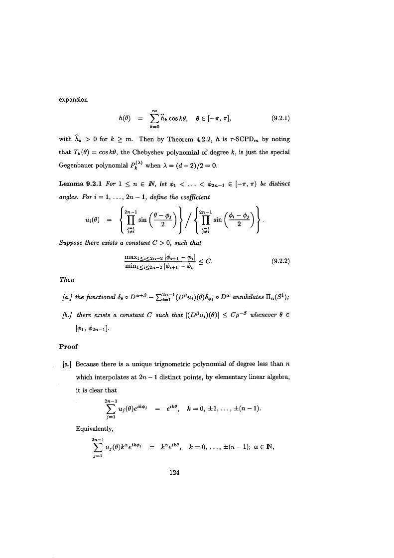
expansion

ooW ) = ^/ifcCosA:^, 9 G [—7 r, 7r], (9.2.1)

k=0

with hk > 0 for k > m . Then by Theorem 4.2.2, h is r-SC PD m by noting

th a t Tk{9) = coskO, the Chebyshev polynomial of degree k , is just the special

L e m m a 9 .2 .1 For 1 < n € IN, let fa < . . . < (f>2n - i £ [—t t , t t ) be distinct

angles. For i = 1, . . . , 2 n — 1, define the coefficient

Suppose there exists a constant C > 0, such that

m a x i i\ ~

Then

[a.] the functional do ° D a+f3 — ° D a annihilates IIn (5 1);

[b.J there exists a constant C such that \ ( D /3Ui )(9) \ < Cp~& whenever 9 E

[<t> 1> 0 2 n —l ] •

P ro o f

[a.] Because there is a unique trignometric polynomial of degree less than n

which interpolates a t 2n — 1 distinct points, by elementary linear algebra,

it is clear th a t

Gegenbauer polynomial p j ^ when A = (d — 2 )/2 = 0.

2 n — 1

Y Uj(6)eik*s = eike, k = 0, ± 1 , . . . , ± ( n - 1).

Equivalently,2 n — 1

124

which in turn is equivalent to

2 n —1

(S0 o D a ~ Y , U j W t i ° D a, p ) = 0, (9.2.3)

for every p E n n(Sd x). Therefore, for each p E I!^ # 1),

2 n —1

✓7/3 2 n —1

= - E “ j(» )d “p(«j)]

= o,

using (9.2.3) above.

[b.] This is obvious by (9.2.2) and the basics for differentiations. ■

L e m m a 9 .2 .2 Let f E C n [—e, e] for some 0 < e < 7r/2. Then, for x E [—e, e]

we can write f in the form

n —1

f (x ) = sin* £ + # „ ( / , a;), (9.2.4)k=o

where, for j = 0, . . . , n — 1,

P ro o f

Firstly, if g E C n [—5, (5] for some S > 0 then g has the following Taylor series

expansion with remainder:

We can differentiate this to see that, for j = 1, . . . , n — 1,

125

so th a t by the uniqueness of Taylor series expansions,

rkHf f ’ t) = (9.2.5)

Of course, for s G C J [—6, <5], j = 1, . . . , n — 1,

\rj(s, x ) | < C ' | | a ( j ) | | 00 , [ _ i , j ] ® j . ( 9 . 2 . 6 )

Let g(t ) = / ( s in - 1 1), t G [—sine, sine]. Then g G C n [—sine, sine], and, for

j = 1, . . . , n - 1,

l l s 0 ) I U [ — sine , sine] ^ C E l l / (i>I U , [ - , , « ] • ( 9 - 2 . 7 )i=l

For x G [e, e],

f ( x ) = g( sinx)

v - % (fc)(0) . fc / • x= 2 ^ — — sin x + r n(#, sinx).k=0

Thus / has an expansion of the form (9.2.4), where

Rn( f , x) = rn (g, sinx).

Differentiating the last equation we have

jR n H f , x ) = sinx),

i = o

where U(x), i = 1, . . . , j is a trigonometric polynomial of degree i, independent

of g. Thus, recalling (9.2.5) and (9.2.6),

\ R n H f , x ) \ = 1 2 ^ ^ ( x ) r n_i (^(t), sinx)i=0

< C E H ^ ) I U [ - S i n e , s i n e ] | s i n x | n - i=G

i= 1

using (9.2.7). ■

126

T h e o re m 9.2 .3 Let the r-SC PD m function h have Fourier series expansion

(9.2.1) and be 2 r -times continuously differentiable on [—7r, it]. Given the set A

of Hm (S 1)-admissible distributions, assume that A contains a subset

= {L x = <5* o D a , . . . , L 2n- i = o D a } € £'t ,

where n > max{2r, m }, a G IN, and —tx < <f>i < . . . < <f)2n~i < ft- F°r f £ Ch,

let s be the radial basis function Hermite interpolant to f on A, as defined by

(9.1.1). Then for any a < (3 < t , there exists a constant C > 0, such that

| P ' 3( / - s) ] W | < C | | / | U p t - ' 3, (9.2.8)

for all sets {<j>i , . . . ,(f>2n- i } satisfying (9.2.2) and 9 G [4>i, </>2n-i]-

P ro o f

Defining Uj(9), j = 1, . . . , 2n — 1, as in Lemma 9.2.1 and using [a.] of the

Lemma, the distribution2n—1

Tp = 6e o D t - Y , Z ^-« (u j(# )) L ,3=1

annihilates IIn (5 1) and hence n m(5 1). By Theorem 9.1.1,

- *)| < ||2> » ft||fc||/||ft.

We establish our error estim ate by bounding \\Tp * h\\h- Since h is 2r-times

differentiable on [—7r, 7r], and even,

h =k=0 '■

Hence, setting Cj = —D ^ ~ aUj(9), j = 1, . . . , 2n — 1, and Co = 1,

\\T(3*h\\l = [T(3, Tp * h]

= [T*,[T*,h(<l>-i,))]

= [T*, [T$, R e r ih ,* - * ) ] ]2n—1

= °ic> > R ^ h ’ * - ■wi] >i, j =0

127

where we have used the fact th a t Tp annihilates polynomials I l2T_ i ( 5 1). Using

Lemma 9.2.2 we see th a t

m * h \ \ i2 n —l 2 n —1

= E ciCjUgrHh, <fi - 4>i) - 2 E h - e)i ,j= 1 J=1

2r f 2n—1

^ c E l l ^ l U ^ . J E l ( I ^ - “«i)(9)ll(D', - “«j)(9)ll«i - 0il2T °fc = l i , j = l

2 n —1

i= i

< C E l l ' > W IU[-.,elP2T- 2'5,fc = l

where we have used Lemma 9.2.1 [b.] in the last line above, and Lemma 9.2.2

in the penultim ate line. Thus,

\\Tff * A||fc < C pr-e . m

T h e o re m 9 .2 .4 Further to the assumptions of Theorem 9.2.3, we assume that

{Sek o D k}%~Q C A in { L 1} . . . , L N}, where fa < 9k < fa n- i , k = 0, . . . , a - 1.

Then for all 0 < 7 < a, we have

\[ IT U - «)](0)| < C \\f\\hpr - ' . (9.2.9)

P ro o f

Firstly, from the mean value theorem, we know that

[ D a - \ S ~ * W ) = - » ) ] (« . - i ) + (» - 9 « - i ) [ U “( / -«)](&).

where £0 6 [19, 0a-\] C [fa, fan-i}- The first term on the right hand side is

zero as it is one of the interpolation conditions, and the second is bounded

by CppT~a = CpT~a+1 using the last theorem. We obtain the full result by

repeating the above argument for 7 = a — 2 , . . . , 0 successively. ■

128

Since Lagrange interpolation is a special case of Hermite interpolation, we

have

C o ro lla ry 9 .2 .5 Let the SCPDm function h be defined by (9.2.1) and be 2r -

times continuously differentiable on [—7r, 7r]. Let X = {0i, . . . , 9n } € [—n, n)

be the distinct interpolation points. Let f G Ch and s be the radial basis function

Lagrange interpolant, that is, s has the form

N

h(d(9, 9j ) ) +q(x ) , (9.2.10)3= 1


s(0i) = f ( d i), i = l , . . . , N , (9.2.11)

where q G n m_i and ciP(^i) = 0 for all p G n m(5 1). I f

max \ 9 i + i - 9 i \ K pi= 1, N —1

for some constant K , then there exists a constant C > 0, independent of p and

9, such that, for each 9\ < 9 < 9n ,

l /W - s(0)l < c\\f\\hp \ (9.2.12)

9.3 Convergence rate on 5d_1, d > 2

Let

OOh = <9-3-13)

k=o

be such th a t

hk = o { i l + k ) - 2vj3{k,d)-1^, with 2v > 2 t + ( d — 1). (9.3.14)

129

Here /3(k,d) is defined by (2.2.25). By Theorem 2.2.10 and Corollary 2.2.13, for

each fixed x E S d~1, h{x •) is 2r-times continuously differentiable, and for all

distributions L, T E £ ', the convolution [L, T * h] is well-defined.

Let L be a pseudo-differential operator of order r < r with symbol L kj = L k,

(see Definition 2.2.31 for definition). T hat is,

L(Yk,j) = L kYkJ (9.3.15)

for all spherical harmonics Ykj , such th a t for k > 0,

C ik r < \Lk\ < C2kr ,

for some positive constants C\ and C2. It is obvious that

L n Jfc(5 d- 1) C n fc(5 d_1). (9.3.16)

Let Hl : S d~x x S d~l i-» 1R, be defined by

M £ , V) “ L ^ L ^ r i ) . (9.3.17)

By the Addition Formula (2.2.26),

hL(S,r>) = t fL 'h t t r i )oo

= ’£ ,h (k )L < L ’>Pix)( Wk=z 0

oo dk

k = 0 j —Q

oo dk= EMW(M)E£‘r*. )Mk = 0 j = 0

oo dk= E k w i m d) E (oWmk=Q j = 0

OO

k = 0

Hence /&£,(£, 77) depends only on the scalar product of £ and 77, th a t is, hx,(£, 77) =

hi(^ri) for some function Hl on [—1, 1]. Note th a t since L is a pseudo-differential

130

operator of order r < r and h € H 2u satisfies (9.3.14), it follows by Corollary

2.2.13 th a t hi, is (2r — 2r)-times continuously differentiable.

We will only consider distributions generated by such an pseudo-differential

operator. Many often used operators belong to this category. Some examples

are:

• the Laplace-Beltrami operator A* with symbol —k(k + d — 2);

• the differential operator (—A* + l /4 ) 1/ 2 with symbol ( k ( k+d—2 )+ l /4 )1/2.

For more examples, see for example [13] and the references therein.

L e m m a 9.3 .1 Let X = {xi, . . . , x n} be a set of points on 5 d_1 unisolvent with

respect to Urn(Sd~1), with n = dirnnm(5d_1). Let p i, . . . , p n be the unique

polynomials such that Pi(xj) = Si j , i, j = 1, . . . , n. Then for every x € 5 d_1,

we have

Nn

Tx Sx Pi(x)SXi € £ m T. i= 1

[2.] Let r < r . Let L be the pseudo-differential operator of order r < t , as

above. Then the functionaln

T i 6 £'m,r - (9.3.18)i= 1

P ro o f

First we prove [1.]. Obviously, for every pj, j = 1, . . . , n, we haven

[Tx , p j ] = [Sx ~ ^ 2 p i ( x ) S Xi, pj^ i—1

n

= P j i x ) - ^ P i { x ) p j { X i ) i = l

n

= Pj{x)

which proves [1.]. For statem ent [2.], note th a t if p G n m(S d 1), then q =

L (p ) G n m(S,d" 1). Hence

[ x f , p ] = [ r „ 4] = o. ■

L em m a 9 .3 .2 Under the assumptions and notations of Lemma 9.3.1,

, T y * h ] = (9.3.19)

P ro o f

We need only prove the case when Tx = Sx , and then the conclusion follows. It

is obvious th a t

[Sx O L, (Sy o L) * h ] = L^L vh(^r}) Il£=® , rj=y

= [<5®, Sy * Hl ]. ■

Now we can state our main theorem in this section.

T h e o re m 9 .3 .3 Let the 2r-times continuously differentiable basis function h

and the pseudo-differential operator L be defined as above. Assume the inter

polation distribution set A = {Li , . . . , L m } contains a subset

Ai := {Li = 5Xi o L : i = 1, . . . , N }, N < M

such that the supporting set X := {x \ , . . . , x ^ } of Ai satisfy the following

inequality,

min max xx i > 1 — p, (9.3.20)xesd- i x i e x ~

for a sufficiently small 0 < p < 1. Let s be the Hermite radial basis interpolant,

i.e.,

M

s = ^ T c j L j * h + p , pG n m(5 d_1)j =i

132

satisfying

[Li, s] = [Li, f], i = 1, . . . , M,

andM

^ 2 ^ = 0’ f ° r ttU P G n m (5d-1).3= 1

Then for every x € 5 d_1, we have

\ L ( f - s ) ( x ) \ < C \ \ f \ \ hpT-r , (9.3.21)

where C > 0 is a constant independent of p.

R e m a rk 9 .3 .4 When L = 1 and r = 0, Theorem 9.3.3 is just [15, Theorem

3.2].

P r o o f o f T h e o re m 9.3 .3

Let k = 2r . From [15], we know th a t for each x € 5'd_1, there is a 11* (£ d-1)-

unisolvent subset X q := {x±, . . . , x n } C X , with n = dimlljfc(5d_1), such that

1 — XiX < Cp and 1 — XiXj < Cp for *, j = 1, . . . , n. Let {p*, i = 1, . . . , n} be

the unique harmonics in E[jk(5d-1) such th a t Pi(xj) = Si j , i , j = 1, . . . , n.

Let the distribution

L0 = 5x o L, (9.3.22)

and let Tx and T f 1 be as defined in [1.] and [2.] of Lemma 9.3.1, respectively.

Then we have, by Theorem 9.1.1 and Lemma 9.3.2,

|L (f - s)(x)| = |[L0, / - * ] ! < \\Tt * ftlUII/IU-

Note th a t

\ \ T i * h \ \ l = [T xL , T ^ h ] = [Tx , T x * h L],

by Lemma 9.3.2. As pointed out previously, hi, is (2 r — 2r)-times continuously

differentiable. By [15, Theorem 3.2 ], we have

[Tx , T x * h L] < C p 2<T- ' \

133

for some constant C > 0 independent of p. Since x is an arbitrary point on

S d~x, the inequality (9.3.21) holds. ■

As an application of this result, let us examine a boundary value problem

(BVP) of potential theory,

f A U = 0 in H .\ a (d U /d v ) + 8U = / on 90 .

Here

n = s 2

is the unbounded outer space with boundary dCl = S 2. Let Sf be the closure

of S 2. Let the ou ter harm onics

H k,i{x) = { l l \ x \ f + lYk d { ^ X x e S ? . (9.3.24)

Let nm(Se2) be the space consisting of combinations of H k j for k = 0, 1, . . . , m —

1; j = 1, . . . , dfc. Let h be the r-SC PD m function on S 2. Let Ch be the ad

m issible Hilbert space defined in Section 7.2.2. That is

OO flfc

Ch = {/ = £E \ h< ook = 0 j = 1

Let

oo dk

c* = { ^ = £ £ * . ' ^ ( 0 ) I ll/ll* <«>}• (9 -3-25)k = 0 j = 1 1 1

It is also a Hilbert space with the norm inherited from Ch', see [13, Equation

(22)]. Furthermore, there exists a positive D > 0, such th a t

sup |F (x )| < D sup \T(F)(x)\ , (9.3.26)x€Sf xeS'2

for every continuous functional T on Ch', see [13, Equation (41)].

134

By the classical analysis of potential theory, the BVP (9.3.23) can be con

verted into a pseudo-differential equation: find U such th a t L(U) = f for some

pseudo-differential operator L , see for example [31]. If U £ Ch, then we can

approximate the solution U by the radial basis function Hermite interpolant.

T h e o re m 9.3 .5 Let the r-SCPD m function h be as in Theorem 9.3.3. Suppose

that the B V P solution U of (9.3.23) belongs to Ch- Let X := {aq, . . . , xtv} C S 2

satisfy

min max xxi > 1 — p, (9.3.27)x€S2Xi€X ~

for a sufficiently small 0 < p < 1. Let L be a pseudo-differential operator of

order r with symbol Lk- Let Li = SXi o L . Let the interpolant

N ___

s = ^ 2 cjLj * h + p, p e n m (S2)3=1

satisfying

[Li , s \ = [Li ,U], i = l , . . . , N ,

andN ___

T , Cj[Lj, p] = 0, for all p £ U m (S2).3= 1

Then s is an approximation to the B V P solution U in (9.3.23), satisfying

sup |*7Or) - s (x) | < C p T~r , (9.3.28)x€zS2

for some constant C > 0.

P ro o f

Note th a t when restricted to S 2, each function F G Ch belongs to Ch, by (9.3.25).

Thus by Theorem 9.3.3, for each x G 5 2,

\[SX o L, U — s]\ = |L(U - *)(*)! < C pT~r ,

135

for some constant C > 0 independent of x and p. Combining with (9.3.26) we

have

sup \U(x) — s(x)| < D sup \L(U)(x)\xesi xeS2

< c PT~r . m

R e m a rk 9 .3 .6 We refer the reader to [31] for a detailed analysis of the above

theorem. In the forthcoming paper, the author and Dr Levesley [36] have a more

complete and detailed discussion on the convergence rate of Hermite interpola

tion on 5 d_1 under more general conditions.

136

Bibliography

[1] N. Aronszajn, Theory of reproducing kernels, Trans. Amer. Math. Soc.,

Vol 68 (1950), 337-404.

[2] M. Atteia, Hilbertian Kernels: Spline Functions, Studies in Computa

tional M athematics IV, North Holland, 1994.

[3] K. Ball, Invertibility of Euclidean matrices and radial basis interpolation,

J. Approx. Theory 68 (1992), 74-82.

[4] K. Ball, N. Sivakumar and J. D. Ward, On the sensibility of radial basis

interpolation with respect to minimal separation distance, Constr. Approx.

8 (1992), 401-426.

[5] A. Yu. Bezhaev and V. A. Vasilenko, Variational Spline Theory, Bulletin

of Novosibirsk Computing Center, Special Issue 3-1993, NCC Publisher,

Novosibirsk, 1993.

[6] B. J. C. Baxter, Norm estimates for inverses of distance matrices, in

M athematical Methods in CAGD, Academic Press, New York, T. Lyche

and L. L. Schumaker (eds.), (1992), 13-18.

[7] B. J. C. Baxter, Norm estimates for inverses of Toeplitz distance matrices,

J. Approx. Theory 79 (1994), 222-242.

137

[8] B. C. Carlson, Special Functions of Applied Mathematics, New York, Aca

demic Press, 1977.

[9] W. F. Donoghue, Distributions and Fourier transforms, Academic Press,

New York, 1969.

[10] J. Duchon, Splines minimising rotation-invariant semi-norms in the So

bolev spaces, in Constructive Theory of Functions of Several Variables,

Lecture Notes in M athematics 571, eds. W. Schempp and K. Zeller,

Springer-Verlag (Berlin), (1977), 85-100.

[11] J. Duchon, Sur I’Erreur d ’Interpolation des Fonctions de Plusieurs Vari

ables par les D m-splines, RAIRO Analyse Numerique 12 (1978), 325-334.

[12] N. Dyn, F .J. Narcowich, and J. D. Ward, Variational principles and

Sobolev-type estimates for generalised interpolation on a Riemannian

manifold, preprint, 1996.

[13] W. Freeden, A spline interpoaltion method fore solving boundary value

problems of potential theory from discretely given data, Numer. Methods

for Differential Equations 3 (1987), 375-398.

[14] M. Gasca and J. I. Maeztu, On Lagrange and Hermite interpolations in

Mn , Numer. M ath. 39 (1982), 1-14.

[15] M. von Golitschek and W. A. Light, Interpolation by polynomials and

radial basis functions on spheres, preprint 1997. To appear in Constr.

Approx.

[16] I. M. Gel’fand and N. Ya. Vilenkin, Generalized functions, Vol. 4, Aca

demic Press, New York, 1964.

[17] I. M. Gel’fand and N. Ya. Vilenkin, Generalized functions, Vol. 1, Aca

demic Press, New York, 1964.

138

[18] M. Golomb and H. F. Weinberger, Optimal approximations and error

bounds, in On Numerical Approximations, ed. R. E. Langer, University of

Wiscosin Press (Madison), (1959), 117-190.

[19] K. Guo, S. Hu and X. Sun, Conditionally positive definite functions and

Laplace-Stieltjes integrals, J. Approx. Theory 74 (1993), 249-265.

[20] R. Hardy, Multiquadric equations of topography and other irregular sur

faces, J. Geophysics Re. 76 (1971), 1905-1915.

[21] K. Jetter, S. D. Riemenschneider and Z. Shen, Hermite interpolation on

the lattice grid, SIAM J. Math. Anal. 25 (1994), 962-975.

[22] P. Kergin, A natural interpolation of C k functions, J. Approx. Theory 29

(1980), 278-293.

[23] Pierre-Jean Laurent, Approximation et Optimisation, Hermann, Paris,

1972.

[24] J. Levesley, W. Light, D. Ragozin and X. Sun, Variational theory for

interpolation on spheres, preprint, (1996).

[25] J. Levesley, Z. Luo and X. Sun, Norm estimates of interpolation matrices

and their inverses associated with strictly positive definite functions, pre

print (1996). To appear in Proc. Amer. Math. Soc.

[26] W. Light and W. Cheney, Interpolation by periodic radial basis functions,

J. Math. Anal. Appl. 168 (1992), 112-130.

[27] W. Light and H. Wayne, Error estimates for approximation by radial basis

functions, in Approximation Theory, Wavelets and Applications, S. P.

Singh (ed.), Kluwer Academic Publishers, (1994), 215-246,

139

[28] W. Light and H. Wayne, Spaces of distributions and interpolation by radial

basis functions, University of Leicester Technical Report 1996/32.

[29] W. Light, Interpolation by translates of a basis function, in M ultivariate

Approximation and Splines, G. Nurberger, J. Schmidt, and G. Walz (eds.),

(1997), 129-140.

[30] R. A. Lorentz, Multivariate Birkhoff Interpolation, Lecture Notes in M ath

ematics, Vol. 1516, Springer-Verlag, Berlin, 1992.

[31] Z. Luo, On spherical spline method for a boundary-valued problem of po

tential theory: well-posedness, stability and convergence rate, preprint,

1998.

[32] Z. Luo and J. Levesley, Error estimates and convergence rates for vari

ational Hermite interpolation, J. Approx. Theory 95 (1998), 264-279.

[33] Z. Luo and J. Levesley, On the conditioning of interpolation by strictly

conditionally positive definite functions on sphere, Numer. Func. Anal,

and Opt. 19 (1998), 849-871.

[34] Z. Luo and J. Levesley, Convergence Rate of Hermite Interpolation on

Spheres: Variational Approach, Technical Report 1997/10, University of

Leicester.

[35] Z. Luo, Strictly positive definiteness of Hermite interpolation on spheres,

to appear in Advances in Comp. Math.

[36] J. Levesley and Z. Luo, Error estimate for Hermite interpolations on

spheres, Technical Report 1998/16. Submitted to Advances in Compu

tational M athematics.

[37] W. R. Madych and S. A. Nelson, Multivariate interpolation and condi

tionally positive definite functions, Approx. Theory Appl. 4 (1988), 77-89.

140

[38] W. R. Madych and S. A. Nelson, Multivariate interpolation and condi

tionally positive definite functions II, Math. Comp. 54 (1990), 211-230.

[39] J. Meinguet, Multivariate interpolation at arbitrary points made simple,

Z. Angew. Math. Phys. 30 (1979), 292-304.

[40] I. P. Natanson, Constructive Function Theory, Vol. I, Ungar, New York,

1964.

[41] V. A. Menegatto, Strictly positive definite functions on spheres, preprint

(1992).

[42] V. A. Menegatto, Strictly positive definite functions on the circle, preprint

(1992).

[43] V. A. Menegatto, Strictly positive definite kernels on the Hilbert space,

preprint (1992). To appear in Applicable Analysis.

[44] C. A. Micchelli, Interpolation of scattered data: distance matrices and

conditionally positive definite functions, Constr. Approx. 2 (1986), 11-22.

[45] C. Muller, Spherical Harmonics, Springer-Verlag, Berlin, 1966.

[46] F. Narcowich, N. Sivakumar, and J. D. Ward,, Stability results for

scattered data interpolation on Euclidean spheres, Adv. in Comp. Math.

8 (1998), 137-164.

[47] F. J. Narcowich and J. D. Ward, Norms of inverses and condition numbers

for matrices associated with scattered data, J. Approx. Theory 64 (1991),

69-94.

[48] F. J. Narcowich and J. D. Ward, Norms o f inverses o f a general class of

scattered data radial basis interpolation matrices, J. Approx. Theory 69

(1992), 84-109.

141

[49] F. J. Narcowich and J. D. Ward, Generalized Hermite interpolation via

matrix-valued conditionally positive definite functions, M ath. Comp. 63

(208), (1994), 661-687.

[50] F. J. Narcowich, Generalised Hermite interpolation and positive definite

kernels on a Riemannian manifold, J. Math. Anal. Appl. 190 (1995), 165-

193.

[51] M. J. D. Powell, The uniform convergence of thin plate spline interpolation

in two dimensions, Numer. Math. 88 (1), (1994), 107-128.

[52] A. Ron and X. Sun, Strictly Positive Definite Functions on Spheres in

Euclidean Spaces, Computation of Mathematics, Vol. 65 (216), (1996),

1503-1530.

[53] R. Schaback, Error estimates and condition numbers for radial basis func

tion interpolation, Advances in Computational Mathematics 3 (1995),

251-246

[54] R. Schaback, Lower bounds for norms of inverses of interpolation matrices

for radial basis functions, J. Approx. Theory 79 (1994), 287-306.

[55] I. J. Schoenberg, Positive definite functions on spheres, Duke M ath. J. 9

(1942), 96-108.

[56] M. Schreiner, On a new condition for strictly positive definite functions

on spheres, Proc. Amer. Math. Soc. 125 (1997), 534-539.

[57] E. M. Stein and G. Weiss, Introduction to Fourier Analysis on Euclidean

Spaces, Princeton Univ. Press, Princeton, NJ, 1971.

[58] R. S. Strichartz, A Guide to Distribution Theory and Fourier Transforms,

Boca Raton, London, CRC, 1994.

142

[59] X. Sun, Scattered Hermite interpolation using radial basis functions, Lin

ear Algebra and its Applications 207 (1994), 135-146.

[60] X. Sun, Norm estimates for inverses of Euclidean distance matrices, J.

Approx. Theory 70 (1992), 339-347.

[61] X. Sun, Conditionally positive definite functions and their application to

multivariate interpolation, J. Approx. Theory 74 (1993), 159-180.

[62] X. Sun and E. W. Cheney, Fundamental sets of continuous functions on

spheres , Constr. Approx. 13 (1997), 245-250.

[63] G. Szego, Orthogonal Polynomials, American M athematical Society Col

loquium Publications, Vol XXIII, Amer. Math. Soc., R. I., Providence,

1939.

[64] Z. Wu, Hermite-Birkhoff interpolation of scattered data by radial basis

functions, Approx. Theory Appl. 8 (1992), 1-10.

[65] Z. Wu and R. Schaback, Local error estimates for radial basis function

interpolation o f scattered data, IMA J. Numer. Anal. 13 (1993), 13-27.

[66] Y. Xu and E. W. Cheney, Strictly positive definite functions on spheres,

Proc. Amer. M ath. Soc. 116 (1992), 977-981.

143

multivariate hermite interpolation in euclidean space … · multivariate hermite interpolation in...

Documents