the influence of thruster dynamics on underwater vehicle ...bachmayer/eng9095-webpage/... · the...

IEEE JOURNAL OF OCEANIC ENGINEERING, VOL. 15, NO. 3, JULY 1990 167

The Influence of Thruster Dynamics on Underwater Vehicle Behavior and Their Incorporation Into

Control System Design

Abstmct-The system dynamics of underwater vehicles can he greatly influenced by the dynamics of the vehicle thrusters. In this paper a nonlinear parametric model of a torque-controlled thruster is developed and experimentally confirmed. The model shows that the thruster behaves like a sluggish nonlinear filter, where the speed of response depends on the commanded thrust level. A quasi-linear analysis utilizing describ ing functions shows that the dynamics of the thruster produce a strong bandwidth constraint and a limit cycle, both of which are commonly seen in practice. Three forms of compensation are tested, utilizing a hybrid simulation which combined an instrumented thruster with a real- time mathematical vehicle model. The first compensator, a linear lead network, is easy to implement and greatly improves performance over the uncompensated system, but does not perform uniformly over the entire operating range. The second compensator, which attempts to cancel the nonlinear filtering effect of the thruster, is effective over the entire operating range but depends on an accurate thruster model. The final compensator, an adaptive sliding controller, is effective over the entire operating range and can compensate for uncertainties or the degradation of the thruster.

I. INTRODUCTION

HE AUTOMATIC control of underwater vehicles repre- T sents a difficult design problem due to the nature of the dynamics of the system to be controlled. Controllers based on simple models of vehicle mass and drag usually yield dis- appointing performance. In this paper, it is shown that for a wide class of vehicles, the dynamics of the thrusters dominate the control problem and must be properly considered to obtain good results.

The general underwater vehicle control system design problem includes a variety of nonlinearities and modeling uncertainties. These include hydrodynamic nonlinearities, inertial nonlinearities, and problems related to coupling between the degrees of freedom [l], [2]. Additionally, the ability of thrusters to produce force is greatly influenced by axial- and cross-flow effects. These types of nonlinearities are especially prominent at high speed.

Manuscript received January 6, 1990; revised March 1990. This work was supported by the ONR under Contract Nos. N00014-86-C-0038 and N00014-88-K-2022, and by ONR Grant N00014-87-J-1111. This paper represents Woods Hole Oceanographic Institution Contribution Number 7307.

D. R. Yoerger and J. G. Cooke are with the Deep Submergence Labora- tory, Department of Applied Physics and Ocean Engineering, Woods Hole Oceanographic Institution, Woods Hole, MA 02543.

J.-J. E. Slotine is with the Department of Mechanical Engineering, Mas- sachusetts Institute of Technology, Cambridge, MA 02139.

IEEE Log Number 9036202.

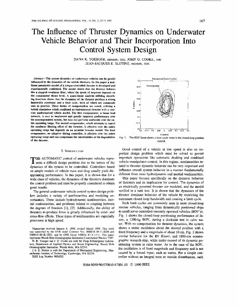
Estimated and Desired Position

O2 7 -I o,,5 1 Desired position

-0.15 1 -0.21 ' ' ' ' ' ' ' I

-0.2 -0.15 -0.1 -0.05 0 0.05 0.1 0.15 0.2

X (meters)

The ROV Jason shows a limit cycle when in the closed-loop position control.

Fig. I

Good control of a vehicle at low speed is also an important design problem which must be solved to permit important operations like automatic docking and combined vehicle-manipulator control. In this regime, nonlinearities related to thruster dynamic behavior can be very important and influence overall system behavior in a manner fundamentally different from most hydrodynamic and inertial nonlinearities.

This paper focuses specifically on the dynamic behavior of thrusters and its implication for control. The dynamics of an electrically powered thruster are modeled, and the model verified in a tank test. It is shown that the dynamics of the thruster dominate behavior of the vehicle by restricting the maximum closed-loop bandwidth and creating a limit cycle.

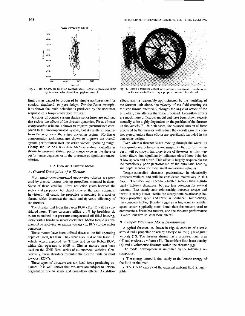
Such limit cycles are commonly seen in most closed-loop marine vehicles, ranging from dynamically positioned ships to small servo-controlled remotely operated vehicles (ROV's). Fig. 1 shows the closed-loop positioning performance of Ja- son, a 1200-kg ROV, during a dockside test in calm water. With no compensation for thruster dynamics, the system shows a stable oscillation about the desired position with a fixed frequency and a magnitude of about 10 cm. Fig. 2 shows similar behavior for the RV Knorr, and 1800-ton oceanographic research ship, while under control of its dynamic positioning system in calm water. As in the case of the ROV, the oscillation is of fixed magnitude and frequency and is not caused by a forced input, such as waves. For a simple controller without an integral term or outside disturbances, such

0364-9059/90/0700-0167$01 .OO 0 1990 IEEE

168 IEEE JOURNAL OF OCEANIC ENGINEERING, VOL. 15, NO. 3, JULY 1990

:“i 4638

I 4632 t:t 4630

4628 1 4626 L 6065

Position of RV KNORR under

6070 6075

X (meters)

‘ID 6080

Fig. 2. RV Knorr, an 1800 ton research vessel, shows a prominent limit cycle when under closed-loop position control.

limit cycles cannot be produced by simple nonlinearities like stiction, deadband, or pure delays. For the Jason example, it is shown that such behavior is produced by the nonlinear response of a torque-controlled thruster.

A series of control system design procedures are outlined that reduce the effects of the thruster dynamics. First, a linear compensation scheme is shown to improve performance compared to the uncompensated system, but it results in nonuni- form behavior over the entire operating regime. Nonlinear compensation techniques are shown to improve the overall system performance over the entire vehicle operating range. Finally, the use of a nonlinear adaptive sliding controller is shown to preserve system performance even as the thruster performance degrades or in the presence of significant uncertainties.

II. A DYNAMIC THRUSTER MODEL

A . General Description of a Thruster Most small-to-medium-sized underwater vehicles are pow-

ered by electric motors driving propellers mounted in ducts. Some of these vehicles utilize reduction gears between the motor and propeller, but direct drive is the most common. In virtually all cases, the propeller is mounted in a duct or shroud which increases the static and dynamic efficiency of the thruster.

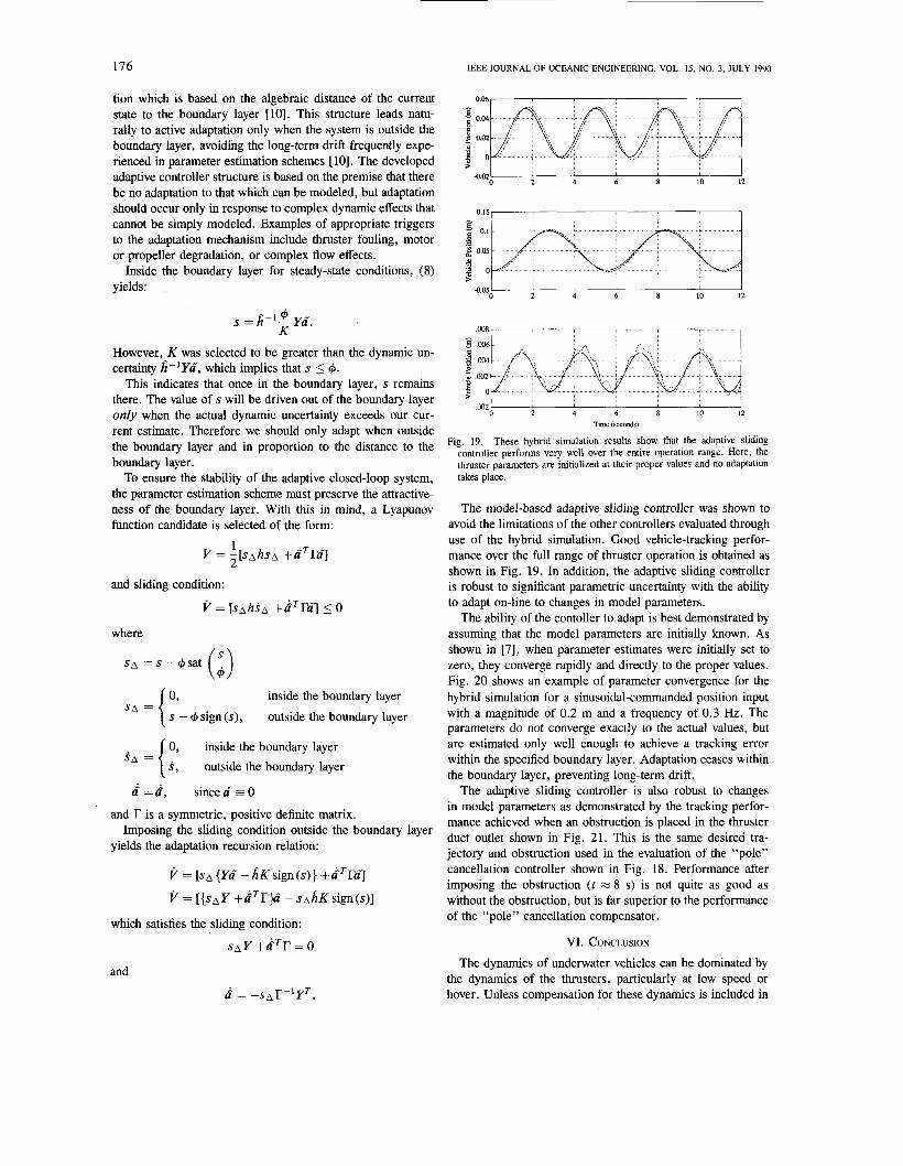
The thruster unit from the Jason ROV (Fig. 3) will be considered here. These thrusters utilize a 1/3 hp brushless dc motor contained in a pressure compensated oil-filled housing, along with a brushless motor controller. Motor torque is commanded by applying an analog voltage ( f 10 V) to the motor controller.

These motors have been utilized down to the full operating depth of Jason, 6000 m. They were also used on the Jason Jr. vehicle which explored the Titanic and on the Robin ROV, which also operates to 6000 m. Similar motors have been used on the UNH Eave series of autonomous vehicles. Con- ceptually, these thrusters resemble the electric units on most

These types of thrusters are not ideal force-producing actuators. It is well known that thrusters are subject to serious degradation due to axial- and cross-flow effects. Axial-flow

low-cost ROV’S.

Fig. 3. Jason’s thrusters consist of a pressure-compensated brushless dc motor and controller driving a propeller mounted in a shroud.

effects can be reasonably approximated by the modeling of the thruster unit alone, the velocity of the fluid entering the thruster shroud effectively changes the angle of attack of the propeller, thus altering the force produced. Cross-flow effects are much more difficult to model and have been shown experimentally to be highly dependent on the position of the thruster on the vehicle [3]. In both cases, the reduced amount of force produced by the thruster will reduce the overall gain of a control system unless these effects are specifically included in the controller design.

Even when a thruster is not moving through the water, its force-producing behavior is not simple. In the rest of this paper it will be shown that these types of thrusters act like nonlinear filters that significantly influence closed-loop behavior at low speeds and hover. This effect is largely responsible for the notoriously poor performance of the automatic heading and depth servoes for most small underwater vehicles.

Torque-controlled thrusters predominate in electrically powered vehicles and will be considered exclusively in this paper. Thrusters with speed-controlled motors have significantly different dynamics, but are less common for several reasons. The steady-state relationship between torque and thrust is nearly linear, while the steady-state relationship between propeller speed and thrust is nonlinear. Additionally, the speed-controlled thruster requires a high-quality angular speed sensor (typically much better than the sensors used to commutate a brushless motor), and the thruster performance is more sensitive to axial flow effects.

B . Lumped Parameter Model Development A typical thruster, as shown in Fig. 4, consists of a static

shroud and a propeller driven by a torque source ( 7 ) at angular velocity (0). The thruster shroud has a cross-sectional area (A) and encloses a volume ( V). The ambient fluid has a density ( p ) and a volumetric flowrate within the thruster (Q) .

The model development is simplified by the following as- sumptions:

The energy stored is due solely to the kinetic energy of the fluid in the duct.

The kinetic energy of the external ambient fluid is negligible.

YOERGER et al.: INFLUENCE OF THRUSTER DYNAMICS ON UNDERWATER VEHICLE BEHAVIOR 169

SHROUD

Fig. 4. Schematic of the thruster. The enclosed volume is V, the crosssec- tional area A, the angular velocity of the propeller is 0, and the applied torque is r .

Friction losses are negligible. Ambient fluid is incompressible. Fluid flow at the thruster intake and exhaust is parallel,

one dimensional, and at ambient pressure. Rotational flow effects are ignored.

Gravity effects are negligible. The thruster is completely symmetric with respect to the

The kinetic coenergy T* of the fluid in the thruster can be

flow direction.

expressed as a state function of the volumetric flowrate Q:

T*(Q) = i p V [:I2. L A

A generalized momentum can be defined as

The above relation is that of an inertia (momentum related by a static constitutive law to the flow [4]) in bond-graph nomenclature with the effort variable r and flow variable Q. r has units of momentum/area and is referred to as the pressure momentum. Since the energy relations are linear, the coenergy and energy have equal magnitudes [ 5 ] , and the kinetic energy T can be expressed as a state function of the pressure momentum I?:

A2 2PV

T ( r ) = -r2.

A power balance yields the following pressure momentum relation;

dT A2 . dt PV - = -rr = or - K Q

where Or represents the power input from the thruster propeller, K represents the exiting kinetic energy per volume, and represents the time rate of change of the pressure momentum.

The exiting kinetic energy per volume K can be expressed as

A 2 r 2 y2 K = - - - 2pv2 - 2 p

where y = A r / V is the fluid momentum per volume within the thruster.

The thruster and ambient fluid are coupled through the con- vected linear momentum, which is equal to the thrust devel-

I : pV/A2

Fig. 5 . Bond graph representing thruster dynamics.

oped:

Thrust = yQ. (3)

Assuming that the propeller does not cavitate, the volumetric flowrate can be related to the thruster/propeller charac- teristics and angular velocity R. The difference between the theoretical and actual advance per revolution of a propeller is referred to as the slip and is typically expressed as a ratio U

as follows:

PA - Q QPA

U =

where p represents the axial distance traveled by the propeller blades with each unit of rotation (1 rad) and is referred to as the pitch,

It follows from the equation above that Q(R) can be expressed as

Q = V P A R (4)

where v = 1 -U and is referred to as the propeller efficiency. From (1)-(4), the following thruster dynamic state and out-

put equations are formed:

Thrust = yQ.

The thruster dynamic state and output equations can be rep- resented topographically in the bond graph of Fig. 5.

If we assume that the propeller efficiency ( v ) , pitch (p), and duct area ( A ) are constant, the thruster dynamic state and output equations may be expressed with the propeller angular velocity R as the thruster dynamic state variable:

Thrust = Apy2p2R101.

Note that the steady-state thrust force is proportional to the input torque, as mentioned earlier.

The normalized step response of the thruster model to torques of 2, 1/3, and 1/4 Nm is presented in Fig. 6, graphically emphasizing the nonlinear dynamics. The thruster presents a more complex control problem than the linear first- order lag associated with most actuators. The thruster time response performance actually degrades as the magnitude of the input decreases. This dynamic behavior, when coupled with other dynamic nonidealities such as a pure delay, could result in the limit-cycle behavior associated with underwater vehicle hover control.

170

" * ' " " 1 1.5 2 2 5 3 3.5 4 4 5 5

Time (seconds)

Fig. 6. The nonlinear nature of the thruster response is illustrated in this set of normalized step responses. The larger the input, the more rapid the dynamics of the thruster.

I I

Fig. 7. The test setup allowed the thruster control voltage to be set from a computer, while the thrust force, flow rate, and propeller speed were logged.

C. Model Summary Using an energy-based physical system approach, a lumped

parameter dynamic model of the thruster was developed. With the propeller angular velocity Cl as the thruster dynamic state, the model and the output equation take the form:

= 07 - (YfllRI

Thrust = CfCllCl;21

where 7 is the input torque, (Y and 0 are constant model parameters, and C f is a proportionality constant.

This model will be used subsequently as a dynamic structure of determining the constant model parameters, and ulti- mately in the design of controller systems to compensate for the thruster dynamics.

III. MODEL VERIFICATION The model was verified using a thruster mounted in a tank

which was instrumented for output force, propeller speed, and output flow velocity. As shown in Fig. 7, the thrust was measured by a load cell, the propeller speed was measured using an electro-optic device similar to a simple optical shaft en- coder but suitable for immersion, and the output flow velocity was measured by an analog electromagnetic current meter.

A series of static and dynamic tests were conducted to con-

8 !

Fig. 8.

80 -

M)-

Fmpeller Angular Velonty Squared

Experimental results show excellent correlation between the steady- state thrust force and the absolute squared propeller speed.

vc (volrs) Fig. 9. The steady-state absolute squared propeller speed is shown expen-

mentally to be a linear function of the applied motor control voltage.

firm the model presented earlier and to determine the specific parameter values a, 0, and Ct . Given the available measure- ments, it was possible to confirm that these corresponded to reasonable values for the physical parameters such as the propeller efficiency and involved volume.

Static tests provided values for Ct and the ratio @/CY. These tests were conducted for thrust in the forward direction only, ignoring the asymmetry of the thruster. Fig. 8 shows a plot of output force versus the absolute squared propeller speed, yielding a value for Ct . Fig. 9 shows absolute squared propeller velocity as a function of applied motor control voltage, which is proportional to torque. This curve yields the ratio p /a . Both plots show excellent agreement to the model. The identified values were:

Ct = 0.022 Ns*

fila = 1.0. io3 v-l s - ~ .

A dynamic test was conducted to determine the individual values of the parameters (Y and @. The thruster was commanded with a random input signal passed through a filter with a 1-hz cutoff. By measuring propeller speed as a function of the applied motor control voltage, least-squares values of CY and 6 were determined:

CY = 0.037

fl = 42 V-' sV2 .


-I 30

0 2 4 6 8 10 12 14 16

Time (sec)

I

Fig. 10. The measured (dashed line) and simulated thrust force (solid line) responses to a random input (dotted line) are shown. The plot shows good agreement and emphasizes the phase lag exhibited by both the real thruster and model.

Note that the ratio of (1.1 . lo3) for /3/a for the dynamic test matches the results of the static tests, even though the dynamic tests included flow in both directions.

Fig. 10 shows the recorded propeller speed data and the simulated response using the identified parameters.

The ratio of these two numbers (1.1 . lo3 V-' sc2 ) compared favorably to the statically determined value of 1.0 . lo3 V-' sc2). Likewise, a least-squares value for C , determined from the recorded dynamic output force and propeller speed yielded a value of 0.019 Ns2, compared to the value 0.022 Ns2 determined from the static tests.

As all the parameters in the model are based on the physical parameters of the motor, propeller, and duct, it is possible to check the experimentally determined values of CY, /3, and C , to see if they make physical sense. The only two physical parameters of the model that are not directly determinable are the involved fluid volume V and the propeller efficiency r ] . Given the experimentally determined parameters a, /3 , and Ct as well as the known physical parameters for propeller pitch ( p = 0.101 m), duct area ( A = 0.0527 m2), and fluid density ( p = loo0 kg/m3), the values of Vand r] can be implied. The computed value of is 0.22, which is reasonable for propellers of this type, and the computed involved fluid volume is 0.016 m3, which is twice the actual volume enclosed by the duct.

In summary, the identification procedure provided good values for the parameters and also supported the basis for the model. Static and dynamic tests were consistent and the identified parameters made physical sense.

IV. EFFECT OF THRUSTER DYNAMICS ON CLOSED-LOOP BEHAVIOR

In this section it will be shown that the thruster dynamic model can be used to explain several difficulties encountered in controlling many types of underwater vehicles. First, a strong constraint on the closed-loop bandwidth is encountered which is much lower than the limit implied by sampling or time delays. Also, the vehicle will exhibit a limit cycle about the desired setpoint.

A quasi-linear approximation of the dynamic model will be used for this analysis. As seen in Fig. 6, the model can be approximated as a first-order system where the time constant is

Nonlinear System

Quasilinear System

7 ::.I p S + J l Q l

Fig. 11. Replacing the absolute squared nonlinearity with a describing function permits the sinusoidal steady-state response of the system to be analyzed.

a function of the input magnitude. Describing functions will be used to approximate the behavior of the system by representing it as a first-order filter which is a function of the magnitude and frequency of a steady input sinusoid. Describing functions are ideal for analyzing a limit cycle, as they apply directly to steady-state sinusoidal conditions.

The block diagram in Fig. 11 shows a thruster model which substitutes a describing function [6] for the absolute-square nonlinearity. For this nonlinearity, the describing function has a gain which is a function of only the magnitude of the input, in this case the propeller speed R. However, the steady-state sinusoidal relationship between the commanded thrust ( F e ) and output thrust force (F , ) is that of a first-order filter for which the break frequency is a function of both the input magnitude and frequency.

Given that the system is first order, the magnitude of the input and output sinusoids are related by

IFt(j4l w -- IFc(jw)I - (U2 + x;h)'12

where the break frequency x t h is a function of the propeller speed R,

Combining these two equations, recalling that the output force F t = CtRIRI, and solving a quadratic yields the break frequency Xth as a function of the input magnitude IFc(jw)I and frequency w :

where

8a 3lr

y = - .

Fig. 12 shows a contour plot of the break frequency x t h for a Jason thruster, using the identified values of a and /3 as a function of the input sinusoid magnitude and frequency w . The break frequency is strongly dependent on the magnitude of the input sinusoid, and weakly dependent on the frequency of the


20

15

10

z 5 P 9 0

1 -5

-10

-I5

0 5 10 15 20 25 30 35 40 45 50 -20

0.2 0.4 0.6 0.8 1 1.2 1.4 1.6 1.8 2

Input frequency (l/s) tune (S)

Fig. 12. The quasi-linear break frequency, as determined from the &crib- ing function analysis, is a strong function of the magnitude of the input and a weaker function of the input frequency.

Fig. 14. This plot of simulated thrust is consistent with the movement of the closed-loop poles shown in Fig. 13. Additionally, the magnitude and frequency of the limit cycle are very close to the values predicted by the describing function analysis.

Desired Clmed-loop

Open-Imp

(a) (b) (C)

Fig. 13. (a) If no thruster dynamics are present, the open-loop poles are easily placed to produce the desired closed-loop response. (b) The unac- knowledged presence of the slow thruster pole results in the actual closed- loop poles moving into the right half plane. (c) The resulting instability causes the thrust level to increase, which speeds up the thruster pole. The thruster pole frequency increases until the pole pair reaches the j w axis to form a pure oscillator.

input sinusoid. For the Jason thruster, the value of the thruster break frequency is less than 2 for all magnitudes, which is certain to wreak havoc with any effort to place the closed-loop poles at a reasonable bandwidth, unless specifically factored into the design.

Now the describing function model can be used to ana- lyze the effect of the thruster dynamics on closed-loop performance. In the simplest case, a single degree of freedom of a vehicle can be described as a pure inertia (Fig. 13(a)). Assume that the goal of the control system design is to place the closed-loop poles at a location specified by the natural frequency Act with a damping ratio { = 0.707. Both position and velocity gains are required to achieve a damped response, and these can be computed algebraically.

However, unless the break frequency of the thruster dynamics is much higher than the desired value of &I, the poles will not move as expected. With the system initially at rest, the thruster action will be low, and the filter break frequency, very low. The presence of the low-frequency pole associated with the thruster dynamics will drive the two other poles into the right half plane. The resulting instability will then increase the magnitude of the input to the thrusters until the filter break frequency increases to the point where the poles lie directly on the j w axis. This process is illustrated in Fig. 13.

This situation describes a classic limit cycle. The resulting oscillation will be of a specific and constant frequency and magnitude that are independent of the initial conditions. The

describing function model can be used to compute approximate values for the magnitude and frequency.

The desired closed-loop system transfer function relates the desired position Xd to the actual position X :

2 X(s> - *n - Xd(s) s2 + 2 r ~ n s +U,’

where on is the desired natural frequency, and r is the desired damping ratio.

Unfortunately, if the thruster dynamics are ignored when the gains are chosen, the following third-order closed-loop transfer function is obtained for the system, including the thruster pole:

k-4 -- - X ( s ) X ~ ( S ) s3 + X ~ S ~ + 2r~thwns +

The value of Ath which puts the two complex poles on the j w axis can be computed by substituting s = jwlc into the characteristic equation and finding the roots, where utc is the frequency of the limit cycle. This calculation yields:

w c = * n

A* = w n / 2 { .

This means that the magnitude of the thruster input will increase until the break frequency of the thruster dynamics reaches a value of w n / 2 r . Recalling (3, the magnitude of the commanded thruster force can be related to the break frequency of the thruster and the thruster command frequency:

Fig. 14 shows that the limit cycle produced a numerical simulation of a single axis of a vehicle the size of Jason Jr., including the full nonlinear thruster dynamics. The magnitude of the commanded thruster signal during the limit cycle is 15.6 N, which corresponds closely to the value of 15.7 N predicted by (6). Likewise, the frequency of the limit cycle corresponds almost exactly tol the desired closed-loop frequency of 11s (period = 2n s).


V. COMPENSATION FOR THRUSTER DYNAMICS

Several controller structures were investigated to overcome the effects of neglecting the thruster dynamics. Recall that there were two bad effects that resulted from neglecting the thruster dynamics: First, overall system bandwidth was limited, and secondly, a limit cycle was produced.

A . Hybrid Simulation A hybrid simulation was used to verify the various controller

designs. The hybrid simulation was an extension of the test setup used to verify the thruster model (see Fig. 7). Rather than just logging the output of the thruster, the measured value was used to drive a real-time numerical simulation of a single degree of freedom vehicle. This permitted the behavior of the actual thruster and its effect on the control loop to be observed while acting on a “pure” vehicle with well-known character- istics. For the controllers that were implemented digitally, the states of the vehicle simulation (x and i ) were made available to the controllers. Additionally, the adaptive sliding controller required the propeller speed measurement 0. A more detailed description of the hybrid simulation is given in [7].

An important limitation of the hybrid simulation is that the thruster does not actually move when the simulated vehicle velocity is nonzero. This means that axial-flow effects are ignored. For this reason, the experiments concentrated on hov- ering and small movements.

The vehicle simulation had the form:

MX = thrust - CoilXI

where M is the effective mass (actual mass plus “added mass”), and CO is the drag parameter. The numerical values used were chosen to represent a single DOF of Jason Jr., M = 340 kg, and CO = 67 Ns2/m2.

A vehicle position controller was implemented which compensates for the vehicle drag with a nonlinear feed-forward term which would produce first-order tracking behavior:

U = c~xlxl- 2 G - X2P

where P = x - x d is the tracking error, U is the computed control force, and X is the desired closed-loop bandwidth.

This control law was used for all the control schemes that follow. However, in each case, a different type of compensation was employed. These compensators operate on the control force U computed by the position controller (which is naive to the existance of the thruster dynamics) to produce an improved overall system response.

B . Lead Compensation Given the resemblence of the nonlinear thruster dynamics

to a first-order system, it is sensible to compensate with a lead network [8]. If the thruster actually behaved like a first-order linear system, a zero could be placed at the frequency of the thruster pole and a complementary pole placed at a higher frequency where it would not interfere with the controller.

Fig. 15 shows the results using a lead compensator compared to the results with no compensation. The lead compensator was implemented in analog form. The time constant

,-. ’ 0.08

0.07 ,‘ \,*.no compensaaon

; ,, , lead compensator , I ’ : ,,

a 01

a 02 2 4 6 8 10 12

Tune (seconds)

Fig. 15. For a sinusoidal tracking task, the lead compensator improved performance considerably over the uncompensated case, as shown in these hybrid simulation results.

2 4 6 8 10 12

Time (seconds) Fig. 16. The effectiveness of the lead compensator diminished as the op-

eration conditions change from those for which the lead compensator was designed. Here, for a low magnitude input, performance has degraded significantly.

selected as representative of the dynamics to be compensated is that observed at low control signals. From Fig. 6, we ob- serve that a 0.75s time constant matches the observed step response at a 1-V control signal. The lead compensator increases the system order to two, and we select our desired dominant poles with an attenuation twice that of the first-order pole and a damping ratio of 0.707. Following the root locus method of [8], the lead compensation pole and zero are placed at - 6.5 and - 2.43, respectively. The resulting improvement due to the addition of lead compensation on the closed-loop system response is shown in Fig. 15.

Fig. 16 shows the results for a trajectory which calls for a much lower level of thrust (resembling hover). The closed- loop response is oscillatory and shows a phase lag not seen when the system is operating closer to the design point.

In summary, the lead compensator represents a substantial improvement over no compensator, but performance degrades substantially if the operating conditions vary greatly from the design point.

C . ‘%le” Cancellation The “pole” cancellation controller is so named because it

compensates for thruster dynamics by canceling the apparent


lag pole with a corresponding “zero.” The corresponding control law which is implemented digitally is of the form:

where U* is the compensated thrust command, and hu(u) is the inverse of the thruster time constant which is chosen as a function of the uncompensated control input U. Note that although the term “pole” us used here loosely, the validity of this time-varying “pole-zero cancellation” can be justified for this first-order system as long as Xu is bounded away from zero.

The pole cancellation method requires the evaluation of the time derivative of the commanded control signal U . The value of U can be determined explicitly if the commanded control signal for the thruster is known a priori, as when there is a predefined force trajectory for the associated vehicle; however, this is not normally the case. The value of U may also be determined by differentiating the vehicle control law, resulting in some terms that are known explicitly and some that may be determined by numerical differentiation. For example, the vehicle control law is

U = -KpZ - K d Z

U = -Kpk - K d i .

The velocity error k is known from the state measurement, and the acceleration error 2 may be determined by numerical differentiation with a known error bound taking the form of a disturbance. Xu( U) represents the location of the apparent first-order

thruster “pole” and is considered a function of the magnitude of the commanded input; X,(u) was determined empirically by matching the step response of a first-order system to the observed thruster step response; X, ( U) was determined for the full range of thruster operation and matched to the functional form:

&(U) = 0.49fi.

In [7], it is shown that this relationship provides a good fit to the observed thruster behavior and that it is consistent with the model identified earlier.

Combining this functional form for X,(u) with the “pole” cancellation differential equation yields the differential equation for the “pole” compensation:

U u *=u+-

0.49fi‘

Fig. 17 shows the hybrid simulation results for the closed- loop system with “pole” compensation. Unlike the lead compensator, the nonlinear compensator provides uniform performance over the entire operating range.

Fig. 18 illustrates a fundamental limitation of the “pole” compensation scheme. In this example, an obstruction was placed in the thruster duct, altering the static and dynamic properties of the thruster. Clearly, the “pole” compensation technique relies on good knowledge of the thruster properties.

J 2 4 6 8 10 12

-0.02‘

: 0 1

P o

B 2 0.05

3 I

2 4 6 8 10 12

2 4 6 8 10 12

Fig. 17. The “pole” cancellation technique provides good performance over a wide range of operating conditions, as shown in these hybrid simulation results.

Time (seconds)

Fig. 18. The “pole” cancellation technique suffers when the actual thruster statics or dynamics differ significantly from the model. Here, a blockage is placed in the flow for the hybrid simulation and control performance degrades significantly.

D . Sliding Controller Unlike the previous two compensators, a model-based com-

pensator can directly take advantage of the previously identified controller model. Given the perfect measurement of the thruster dynamic state and a perfect model, the input torque can be directly computed and applied; however, this computed torque method may quickly fail in the presence of model uncertainty, measurement noise, computational delays, and disturbances.

Analysis of the effects of these nonidealities are further complicated by nonlinear dynamics. The issue becomes one of ensuring that a nonlinear dynamic system remains robust to nonidealities while minimizing tracking error.

One method able to deal directly with system uncertainties is referred to as “Sliding Mode Control” and has received considerable attention in the Soviet literature, where it

YOERGER e/ al.: INFLUENCE OF THRUSTER DYNAMICS ON UNDERWATER VEHICLE BEHAVIOR 175

is applied to the control of linear systems with discontinuous control action. Sliding control theory has been extended to systems with nonlinear systems with continuous control action [9], and has been further extended to included adaptation to system parametric uncertainty [ 101. Application of adaptive sliding mode theory permits precise tracking performance while being robust to modeling errors and disturbances. The controller design presented follows closely the development of sliding controllers in [ 101 and [9].

With the propeller angular velocity R as our thruster state measurement, the thruster dynamic model can be written as

R = p7 - (YRIR1

or

hfi = 7 - c R ~ R ~

where 7 is the input torque, while a and /3 are the thruster parameters.

A sliding surface s (in the example in this paper, a point) is selected based on simple linear dynamics:

s = = 0- f&j

where fld is the desired angular velocity. Perfect tracking is then achieved by the state trajectory remaining at the sliding point (s = 0).

Having selected the sliding point, the condition (referred to as the sliding condition) necessary to constrain trajectories to be directed toward the sliding point must be determined. The sliding condition is satisfied if a quadratic form of s can be established as an Lyapunov-like function of the closed loop system [9]:

1 V = -hs2

2

V = shS 5 0 .

Imposing the sliding condition on the dynamic model and sliding point yields the control law:

s = R

hS = h a = h ( d - Qj)

and substituting the system dynamics:

h i = T - CRlRl - hfid

the best approximation of a continuous control law which would achieve h i = 0 is

? = fRlRl + h & where ( * ) indicates an estimate.

To satisfy the sliding condition despite model uncertainty, a discontinuous control law is required. This can be achieved by adding a term to the approximately continuous control law which is discontinuous across the sliding point:

7 = C R ( R I + A { & -Ksign(s)}

where 1, s > o

-1, s < o sign(s)

and K is selected to be large enough to offset the model dynamic uncertainty, ensuring that the sliding condition remains satisfied.

Although the discontinuous control law provides for perfect tracking despite nonidealities, it exhibits undesirable chattering around the sliding point. Chattering can be avoided by smoothing the control law within a thin boundary of the sliding point [9]. This smoothing introduces behavior which de- parts from the dynamics specified by the sliding surface in the form of a first-order filter in s when inside a region about the sliding surface called the "boundary layer." This can be accomplished by replacing the discontinuous control law term by the continuous term K sat (s/d), where

sign(z), for 121 2 1 { 2 , otherwise sat (2 )

and q5 is the boundary layer width.

the form: Inside the boundary layer, the dynamics of s should take

S + X s = b u

where U is the input, b is the input gain, and X is the bandwidth.

This can be verified by substituting the modified control law inside the boundary layer into the dynamic equation for the sliding point:

hS = 7 - CRlRl - h&

h i = fRlRl +hhd - hK- - CRlRl - h& S

4 S hS = -hK- +Ya" 4

where a = [c hIT, a" a ̂-a is the parametric uncertainty, and Y = [RIRI&].

The dynamics of s can be seen to be first order:

K 4

s + -s = h-lya".

This implies that inside the boundary layer the bandwidth is established by

K 4

with s dynamics driven by the dynamic uncertainty, h-'YG.

trol law:

-

The sliding controller with a boundary layer yields the con-

E. Adaptive Sliding Controller The sliding controller design can be made adaptive to para-

metric uncertainty by coupling it to on-line parameter estima-


tion which is based on the algebraic distance of the current 006

state to the boundary layer [lo]. This structure leads natu- rally to active adaptation only when the system is outside the boundary layer, avoiding the long-term drift frequently expe- rienced in parameter estimation schemes [lo]. The developed

be no adaptation to that which can be modeled, but adaptation

cannot be simply modeled. Examples of appropriate triggers to the adaptation mechanism include thruster fouling, motor or propeller degradation, or complex flow effects.

:I o,02

p 2 4 6 10 adaptive controller structure is based on the premise that there

should occur only in response to complex dynamic effects that

-0.02 12

0 15

3 o 1

.$ 2 005

Inside the boundary layer for steady-state conditions, (8) $ o

yields: 0 05 2 4 6 8 10 12

.. 14 s = h - - Ya". K

However, K was selected to be greater than the dynamic uncertainty h-'Ya", which implies that s 5 4.

This indicates that once in the boundary layer, s remains there. The value of s will be driven out of the boundary layer only when the actual dynamic uncertainty exceeds our current estimate. Therefore we should only adapt when outside the boundary layer and in proportion to the distance to the boundary layer.

To ensure the stability of the adaptive closed-loop system, the parameter estimation scheme must preserve the attractive- ness of the boundary layer. With this in mind, a Lyapunov function candidate is selected of the form:

and sliding condition:

where

0, inside the boundary layer = { s - 4 sign (s), outside the boundary layer

0, inside the boundary layer S, outside the boundary layer

S A =

I 2 4 6 8 10 12

Time (seconds)

Fig. 19. These hybrid simulation results show that the adaptive sliding controller performs very well over the entire operation range. Here, the thruster parameters are initialized at their proper values and no adaptation takes place.

The model-based adaptive sliding controller was shown to avoid the limitations of the other controllers evaluated through use of the hybrid simulation. Good vehicle-tracking performance over the full range of thruster operation is obtained as shown in Fig. 19. In addition, the adaptive sliding controller is robust to significant parametric uncertainty with the ability to adapt on-line to changes in model parameters.

The ability of the contoller to adapt is best demonstrated by assuming that the model parameters are initially known. As shown in [7], when parameter estimates were initially set to zero, they converge rapidly and directly to the proper values. Fig. 20 shows an example of parameter convergence for the hybrid simulation for a sinusoidal-commanded position input with a magnitude of 0.2 m and a frequency of 0.3 Hz. The parameters do not converge exactly to the actual values, but are estimated only well enough to achieve a tracking error within the specified boundary layer. Adaptation ceases within the boundary layer, preventing long-term drift. . .

a" = 6, since a 0 The adaptive sliding controller is also robust to changes in model parameters as demonstrated by the tracking performance achieved when an obstruction is placed in the thruster duct outlet shown in Fig. 21. This is the same desired trajectory and obstruction used in the evaluation of the "pole"

and

yields the adaptation recursion relation:

is a symmetric, positive definite matrix. Imposing the sliding condition outside the boundary layer

cancellation controller shown in Fig. 18. Performance after imposing the obstruction ( t M 8 s) is not quite as good as without the obstruction, but is far superior to the performance of the "pole" cancellation compensator.

V = [sa { ~ a " - L K sign (s)) +Pro2 V = [ { S A Y +hTrp - S A ~ K sign(s)l

which satisfies the sliding condition:

S A Y +Pr = o VI. CONCLUSION

The dynamics of underwater vehicles can be dominated by the dynamics of the thrusters, particularly at low speed or hover. Unless compensation for these dynamics is included in

177 /

YOERGER et al.: INFLUENCE OF THRUSTER DYNAMICS ON UNDERWATER VEHICLE BEHAVIOR

001

0009

0008

WO7

0006

0005

WO4

0003

WO2

0001

0 5 10 15 20 25 30

Tune (seconds)

0 035

0 03

0.025

0 02

0015

0 01

0 005

0 5 10 15 20 25 30

Tune (seconds)

Fig. 20. With the parameters initialized at zero, the adaptive sliding controller shows rapid parameter convergence, after which adaptation ceases.

A quasi-linear analysis utilizing describing functions was performed to investigate the influence of the thruster dynamics on the closed-loop system behavior. The analysis reveals that the thruster dynamics place a strong constraint on the closed-loop system bandwidth and produce a limit cycle. Fur- thermore, the frequency and magnitude of the limit cycle can be precisely predicted.

Three forms of compensation were tested utilizing a hybrid simulation which combined an instrumented thruster with a real-time mathematical vehicle model. The first compensator, a linear lead network, was easy to implement and greatly improved performance over the uncompensated system, but did not perform uniformly over the entire operating range. The second compensator, which attempts to cancel the nonlinear filtering effect of the thruster, was effective over the entire operating range but depends on an accurate thruster model. The final compensator, an adaptive sliding controller, was effective over the entire operating range and can compensate for

uncertainties or degradation of the thruster.

REFERENCES

M. Abkowitz, Stability and Motion Control of Ocean Vehicles. Cambridge, MA: MIT Press, 1969. M. Gertler and G. R. Hagen, “Standard equations of motion for submarine simulations,” Naval Ship R&D Center, Bethesda, MD, NSRDC Rep. No. 2510, 1967. J . Feldman, “Model investigations of stability and control character- istics of a preliminary design of the deep submergence rescue vehicle (DSRV scheme A),” NSRDC Rep., June 1966. D. C. Karnopp and R. C. Rosenberg, System Dynamics: A Unified Approach. New York: Wiley, 1975. S. H. Crandall, D. C. Karnopp, E. F. Kurtz, and D. C. Pridmore- Brown, Dynamics of Mechanical and Electromechanical Systems. New York: McGraw-Hill, 1968. D. Graham and D. McRuer, Analysis of Nonlinear Control Systems. New York: Wiley, 1961. J . G. Cooke, “Incorporating thruster dynamics in the control of an underwater vehicle,” Engineers degree thesis, MIT-WHO1 Joint Pro- gram in Oceanogr. Eng., Woods Hole, MA, Sept. 1989. K. Ogata, Modern Control Engineering. Englewood Cliffs, NJ: Prentice-Hall, 1970. J.-J. E. Slotine, “Sliding controller design for nonlinear systems,” Znt. J. Contr., vol. 40, no. 2, 1984. J.-J. E. Slotine and J . A. Coetsee, “Adaptive sliding controller syn- thesis for nonlinear systems,” Znt. J. Contr., vol. 42, no. 6, 1986. V. I. Utkin, Sliding Modes and their Application in Variable Struc- ture Systems. Moscow: MIR, 1974.

I 5 10 15 20 25 30

Time (seconds)

Fig. 2 1. Unlike the “pole” cancellation technique shown in Fig. 18, the use of an adaptive sliding controller allows the system to maintain performance even when an obstruction is placed in the duct.

the control system, the closed-loop system will be limited in bandwidth and prone to limit cycle. This behavior is seen in the heading and depth control of most commercial ROV’s, and also in the position control of advanced ROV’s and AUV’s.

A lumped parameter model of a torque-controlled thruster shows the dynamics to be nonlinear. The thruster represents a fairly sluggish filter, although the speed of response increases with the magnitude of the thruster input. The lumped parameter model was identified in a test tank using an instrumented thruster from the full ocean depth ROV Jason.

Dana R. Yoerger (M’87) obtained the S.B., S.M., and Ph.D. degrees in mechanical engineering from the Massachusetts Institute of Technology, Cam- bridge.

He is an Associate Scientist at the Woods Hole Oceanographic Institution, Department of Applied Physics and Engineering. His interests are in the areas of underwater vehicles and manipulators. He has published papers on vehicle and tether dynamics, the application of modem nonlinear and adaptive control techniques to underwater vehicles, su-

pervisor control methodologies, and underwater manipulator design and performance. He is a Principal Investigator in the design and implementation of Argo/Jason, an advanced telerobotic system for scientific seafloor survey, and ABE, and autonomous vehicle for long-term monitoring of the deep ocean. He has participated In numerous oceanographic cruises, including the discov-

178

ery of the Titanic, full-scale dynamic testing of the Argo system, and the initial deep-ocean deployments of the Jason vehicle and manipulator.

Dr. Yoerger is a member of the IEEE Oceanic Engineering Society Administrative Committee and of the Editorial Advisory Board of the journal, Mechatronics.

* John G. Cooke completed his undergraduate stud- ies at the U.S. Naval Academy, Annapolis, receiv- ing the Bachelor of Science degree in mechanical engineering, and was commissioned in 1978. In 1989 he received the degree of ocean engineer from the Massachusetts Institute of TechnologylWoods Hole Oceanographic Institution Joint Program in Oceanographic Engineering.

He is a Lieutenant commander in the U.S. Navy. He completed nuclear propulsion and submarine training in 1980 and was assigned to the commis-

sioning crew of the USS Ohio ( G B N 726). He served asEngineering Officer of the commissioning crew of the USS Georgia (SSBN 729) and a Naviga- tor and Operations Officer of the USS San Francisco (SSN 711). LCDR

IEEE JOURNAL OF OCEANIC ENGINEERING, VOL. 15, NO. 3, JULY 1990

Cooke is currently Officer-in-Charge of the U.S. Navy’s nuclear-powered deep-submergence research vessel NR-1.

* Jean-Jacques E. Slotine (S’82-M’83) received the Ph.D. degree from the Massachusetts Institute of Technology (MIT), Cambridge, in 1983.

He is Associate Professor of Mechanical Engi- neering at MIT, Director of the nonlinear Systems Laboratory, Doherty Professor of Ocean Utiliza- tion and CO-Director and CO-Founder of the Cen- ter for Information-Driven Mechanical Systems. His research focuses on applied nonlinear control, robotics, and learning systems. Professor Slotine is the co-author of the textbooks, Robust Analysis

and Control and Applied Nonlinear Control, based on graduate courses he developed at MIT. He is an Associate Editor of several professional journals and is a frequent Consultant to industry and the Woods Hole Oceanographic Institution.

the influence of thruster dynamics on underwater vehicle ...bachmayer/eng9095-webpage/... · the...

Documents