the in format in content of high-frequency data for estimating equity return models
TRANSCRIPT
8/3/2019 The In Format In Content of High-Frequency Data for Estimating Equity Return Models
http://slidepdf.com/reader/full/the-in-format-in-content-of-high-frequency-data-for-estimating-equity-return 1/48
Electronic copy available at: http://ssrn.com/abstract=1895533
Finance and EconomicsDiscussion SeriesDivision of Research & Statistics and Monetary AffairsFederal Reserve Board, Washington, DC
The Information Content of High-Frequency Data for Estimating Equity Return Models and Forecasting
Risk
Dobrislav P. Dobrev and Pawel J. Szerszen2010-45
Z.11
8/3/2019 The In Format In Content of High-Frequency Data for Estimating Equity Return Models
http://slidepdf.com/reader/full/the-in-format-in-content-of-high-frequency-data-for-estimating-equity-return 2/48
Electronic copy available at: http://ssrn.com/abstract=1895533
Finance and Economics Discussion SeriesDivisions of Research & Statistics and Monetary Affairs
Federal Reserve Board, Washington, D.C.
The Information Content of High-Frequency Data for EstimatingEquity Return Models and Forecasting Risk
Dobrislav P. Dobrev and Pawel J. Szerszen
2010-45
NOTE: Staff working papers in the Finance and Economics Discussion Series (FEDS) are preliminarymaterials circulated to stimulate discussion and critical comment. The analysis and conclusions set forthare those of the authors and do not indicate concurrence by other members of the research staff or theBoard of Governors. References in publications to the Finance and Economics Discussion Series (other thanacknowledgement) should be cleared with the author(s) to protect the tentative character of these papers.

8/3/2019 The In Format In Content of High-Frequency Data for Estimating Equity Return Models
http://slidepdf.com/reader/full/the-in-format-in-content-of-high-frequency-data-for-estimating-equity-return 3/48
Electronic copy available at: http://ssrn.com/abstract=1895533
8/3/2019 The In Format In Content of High-Frequency Data for Estimating Equity Return Models
http://slidepdf.com/reader/full/the-in-format-in-content-of-high-frequency-data-for-estimating-equity-return 4/48
The Information Content of High-Frequency Data for
Estimating Equity Return Models and Forecasting Risk
Dobrislav Dobrev, Pawel Szerszen ∗
First version: December 30, 2009
This version: July 25, 2010
Abstract
We demonstrate that the parameters controlling skewness and kurtosis in popular
equity return models estimated at daily frequency can be obtained almost as preciselyas if volatility is observable by simply incorporating the strong information content of
realized volatility measures extracted from high-frequency data. For this purpose, we
introduce asymptotically exact volatility measurement equations in state space form
and propose a Bayesian estimation approach. Our highly efficient estimates lead in
turn to substantial gains for forecasting various risk measures at horizons ranging from
a few days to a few months ahead when taking also into account parameter uncertainty.
As a practical rule of thumb, we find that two years of high frequency data often suffice
to obtain the same level of precision as twenty years of daily data, thereby making our
approach particularly useful in finance applications where only short data samples are
available or economically meaningful to use. Moreover, we find that compared to model
inference without high-frequency data, our approach largely eliminates underestimationof risk during bad times or overestimation of risk during good times. We assess the
attainable improvements in VaR forecast accuracy on simulated data and provide an
empirical illustration on stock returns during the financial crisis of 2007-2008.
JEL classification : C11; C13; C14; C15; C22; C53; C80; G17;
Keywords: Equity return models; Parameter uncertainty; Bayesian estimation; MCMC;
High-frequency data; Jump-robust volatility measures; Value at Risk; Forecasting.
∗Dobrislav Dobrev: Federal Reserve Board of Governors, [email protected]
Pawel Szerszen: Federal Reserve Board of Governors, [email protected]
We are grateful to Torben Andersen, Federico Bandi, Luca Benzoni, Michael Gordy, Erik Hjalmarsson,Michael Johannes, Matthew Pritsker, and Viktor Todorov for helpful discussions and comments. We alsothank conference participants at the 2010 International Risk Management Conference, the 30th InternationalSymposium on Forecasting, the 16th International Conference on Computing in Economics and Finance, aswell as seminar participants at the Federal Reserve Board, Johns Hopkins University, and the Office of theComptroller of the Currency for their feedback. Excellent research assistance has been provided by PatrickMason as well as Erica Reisman and Raymond Zhong. Any errors or omissions are our sole responsibility.
The views in this paper are solely those of the authors and should not be interpreted as reflecting the viewsof the Board of Governors of the Federal Reserve System or of any other person associated with the FederalReserve System.

8/3/2019 The In Format In Content of High-Frequency Data for Estimating Equity Return Models
http://slidepdf.com/reader/full/the-in-format-in-content-of-high-frequency-data-for-estimating-equity-return 5/48
8/3/2019 The In Format In Content of High-Frequency Data for Estimating Equity Return Models
http://slidepdf.com/reader/full/the-in-format-in-content-of-high-frequency-data-for-estimating-equity-return 6/48
1 Introduction
Modeling equity returns is central to risk management, derivatives pricing, portfolio
choice, and asset pricing in general. Continuous time jump-diffusion models succeeding
those pioneered by Merton (1969) and Black and Scholes (1973) are now commonplace.Typically, the inherent time-varying and stochastic nature of continuous market activity is
represented by a combination of persistent and non-persistent latent stochastic volatility
factors. The pronounced asymmetric return-volatility relation in equities, known also as
leverage or volatility feedback effects, is captured by correlated return and volatility inno-
vations. Sudden price revisions due to news and other market surprises give rise to jumps in
returns, while the often abrupt changes in the level of market activity and risk has justified
the introduction of jumps in volatility. The latent nature of volatility in such rich models,
however, poses serious challenges for reliable inference based solely on daily or monthly re-
turn series, even the longest existing ones. It is thus critical to develop estimation methods
exploiting relevant additional information that could help reduce the severe parameter and
volatility estimation uncertainty.
Two different approaches have emerged to improve estimation efficiency in this regard.
The first approach relies on the cross section of option prices over time.1 However, as pointed
out by Eraker, Johannes, and Polson (2003), it is unclear whether the inclusion of option
price data leads to decrease or increase of parameter uncertainty given that the risk premia
embedded in option prices introduce additional parameters, which are typically difficult to
estimate. The second and seemingly more viable approach avoids such complications by
exclusively relying on daily realized volatility measures extracted from nowadays ubiquitous
high-frequency intraday return data.2,3 Our paper contributes to this second line of research
by utilizing high-frequency realized volatility measures within a standard Bayesian Markov
Chain Monte Carlo (MCMC) estimation framework of popular equity return models. In
particular, we take explicitly into account the resulting substantial reduction in parameter
uncertainty and are able to show sizeable economic gains when forecasting risk.
The most closely related studies to our work such as Alizadeh, Brandt, and Diebold
(2002), Barndorff-Nielsen and Shephard (2002), Bollerslev and Zhou (2002), Corradi and
Distaso (2006), Todorov (2009) among others have used classical rather than Bayesian esti-
mation methods and have focused on using high-frequency volatility measures for assessing
the goodness of fit of alternative model specifications without explicitly analyzing the eco-nomic value of reducing parameter uncertainty. These studies have largely ruled out the
1See for example, Chernov and Ghysels (2000), Pan (2002), and Eraker (2004) among others.2Recent surveys of the realized volatility literature include Andersen, Bollerslev, and Diebold (2009),
Bandi and Russell (2007), Barndorff-Nielsen and Shephard (2007), McAleer and Medeiros (2008).3Thorough empirical evidence pointing more broadly towards the value of realized volatility for modeling
equity returns can be found in Andersen, Bollerslev, Diebold, and Ebens (2001).
1

8/3/2019 The In Format In Content of High-Frequency Data for Estimating Equity Return Models
http://slidepdf.com/reader/full/the-in-format-in-content-of-high-frequency-data-for-estimating-equity-return 7/48
simplest known single factor stochastic volatility models with Poisson jumps in returns in
favor of more complex specifications including one or more extra features such as a second
stochastic volatility factor, pronounced non-linearities, jumps both in returns and volatility
(possibly even of infinite activity).4 But rather than reconciling or refining such findings,
our main goal is to go a step beyond specification testing and clearly demonstrate the eco-
nomic gains from harnessing the information content of high-frequency volatility measures
regardless of the underlying model.
To this end, we exploit recent advances in jump robust volatility estimation from high-
frequency data such as Andersen, Dobrev, and Schaumburg (2009), Barndorff-Nielsen, Shep-
hard, and Winkel (2006), Podolskij and Vetter (2009) and references therein to formally
introduce an asymptotically precise volatility measurement equation directly within the
standard state-space representation of popular equity return models estimated at daily or
lower frequency. Then we adopt a standard Bayesian MCMC estimation framework allowing
us to exploit the strong information content of such volatility measurement equation acrossa wide range of models featuring stochastic volatility, leverage effects, and jumps in re-
turns and volatility. In terms of efficiency, our approach considerably improves on Bayesian
estimation methods based on an identical state-space representation at a daily or lower
frequency but without a volatility measurement equation such as Eraker, Johannes, and
Polson (2003) and Jacquier, Polson, and Rossi (2004), among others.5 In terms of gener-
ality, we overcome major limitations of the quasi-maximum likelihood estimation methods
for state-space formulations with volatility measurement equation pursued by Barndorff-
Nielsen and Shephard (2002) who consider non jump-robust realized volatility measures
and Alizadeh, Brandt, and Diebold (2002) who consider non jump-robust and less efficient
range-based volatility measures. In particular, our approach incorporates leverage effects
and jumps, necessary for modeling equity returns, as well as possibly two (one persistent
and one non-persistent) stochastic volatility factors. We also offer an attractive alterna-
tive to existing moment-based estimation approaches such as Bollerslev and Zhou (2002),
Corradi and Distaso (2006) and Todorov (2009) in terms of more fully exploiting the in-
formation content of high frequency volatility measures in various model settings via their
state-space formulations. In particular, unlike these studies, the Bayesian estimation ap-
proach we propose allows us to easily account for parameter uncertainty and demonstrate
the economic gains from using high-frequency volatility measures for model estimation and
risk forecasting across a range of popular equity return models. 6
4Results in the same spirit have been obtained also in studies based solely on daily returns or in com-bination with options data such as Broadie, Chernov, and Johannes (2007). Other non-parametric studiesbased on high-frequency data include Andersen, Bollerslev, and Dobrev (2007), Bandi and Reno (2009).
5Cf. Andersen, Benzoni, and Lund (2002) and Chernov, Gallant, Ghysels, and Tauchen (2003).6As such, our results add to the growing body of evidence showing the economic value of high-frequency
realized volatility measures in finance applications, e.g. Fleming, Kirby, and Ostdiek (2003) among others.
2
8/3/2019 The In Format In Content of High-Frequency Data for Estimating Equity Return Models
http://slidepdf.com/reader/full/the-in-format-in-content-of-high-frequency-data-for-estimating-equity-return 8/48
Our main contributions can be summarized as follows. First, we demonstrate theo-
retically and empirically that the parameters controlling skewness and kurtosis in popular
equity return models estimated at daily and monthly frequency can be obtained almost as
precisely as if volatility is observable by incorporating the strong information content of
realized volatility measures extracted from high-frequency data. In particular, we extend
the empirical findings in Alizadeh, Brandt, and Diebold (2002) by showing that not only
the parameters controlling volatility of volatility but also those controlling leverage effects
can be estimated several times more precisely by exploiting high-frequency volatility mea-
sures. Second, we show that our highly efficient estimates lead in turn to substantial gains
for forecasting various risk measures at horizons ranging from a few days to a few months
ahead when taking also into account parameter uncertainty. In fact, our approach not only
reduces the root mean square prediction error but also shrinks and almost eliminates the
forecast bias, which inevitably arises from the pronounced nonlinearities in the involved
transformation of parameter and volatility estimates. As a practical rule of thumb we findthat two years of high frequency data often suffice to obtain the same level of precision
as twenty years of daily data, thereby making our approach particularly useful in finance
applications where only short data samples are available or economically meaningful to
use. Third, and most important in risk management applications, our simulation results
reveal that risk forecasts stemming from traditional model inference on daily data tend to
be overly conservative in good times (e.g. overestimating risk by as much as 30%) but they
are not conservative enough in bad times (e.g. underestimating risk by as much as 10%).
By contrast, risk forecasts based on our approach to exploiting high-frequency data are
considerably closer to the truth in both bad and good times. Thanks to incorporating the
strong information content of high-frequency volatility measures, we are able to better curb
risk taking exactly when needed the most, i.e. early on in times of crisis, while avoiding
unnecessary overstatement of risk in normal times. Finally, our findings are robust both
across different models and jump-robust volatility measures on high frequency data that
we analyze. This allows us to remain largely agnostic about the best suited ones, while
making a strong case for the potentially large economic value of our approach to using
high-frequency volatility measures in model estimation and risk forecasting or other closely
related finance applications such as derivatives pricing.
The rest of the paper is organized as follows. Section 2 introduces our volatility mea-
surement equations in detail. Section 3 incorporates such equations within the state space
formulation of popular equity return models and develops appropriate Bayesian estimation
methods. Section 4 documents the resulting gains in estimation efficiency and risk fore-
casting accuracy. Section 5 provides an empirical comparison of Value-at-Risk forecasts on
S&P 500 and Google returns during the financial crisis of 2007-2008. Section 6 concludes.
3
8/3/2019 The In Format In Content of High-Frequency Data for Estimating Equity Return Models
http://slidepdf.com/reader/full/the-in-format-in-content-of-high-frequency-data-for-estimating-equity-return 9/48
2 Volatility measurement equations
Jumps in returns have been recognized as an important feature for continuous-time
modeling of equity returns within standard no-arbitrage semimartingale setting. Moreover,
recent progress in non-parametric volatility measurement based on high-frequency intradaydata has made it possible to separate ex-post the daily continuous part of the volatility
process from the daily return variation induced by discontinuities or jumps. Originally pi-
oneered by Barndorff-Nielsen and Shephard (2004), jump-robust volatility estimators with
different asymptotic and finite sample properties have been proposed by Andersen, Dobrev,
and Schaumburg (2009), Barndorff-Nielsen, Shephard, and Winkel (2006), Podolskij and
Vetter (2009) among others. A common feature among these and other high-frequency
volatility estimators is that as the intraday sampling frequency increases, the arising mea-
surement error shrinks to zero and converges to a known mixed normal asymptotic distri-
bution.7
For our purposes, suitable asymptotic results of this kind directly imply asymptotically
precise measurement equations that formally capture the extent to which the continuous and
jump parts of daily total variance become ex-post nearly observable when high frequency
intraday data is available. Such separation of the continuous and jump components of
volatility can be directly utilized in state space form. In this section, we formally introduce
a general form of the jump-robust volatility measurement equations that play a key role in
our approach to estimating models in state space form and allow us to tackle considerably
more general settings than those considered by Alizadeh, Brandt, and Diebold (2002) and
Barndorff-Nielsen and Shephard (2002) in the absence of jump-robust volatility measures
nearly a decade ago.
2.1 Jump-robust estimators of diffusive volatility
On a filtered probability space (Ω, F , (F t)t≥0, P ) we consider an adapted process Y =
Y tt≥0, providing the following jump-diffusion represention of the evolution of the loga-
rithmic price of an asset in continuous time:
dY t = µt dt + σt dBt + dJ t (1)
Here µ is a locally bounded and predictable process, σ is cadlag and bounded away from
zero almost surely, while J is a jump process so that dJ t, whenever different from zero,
7The rate of convergence is typically square-root. It is slower for high-frequency volatility measures thatare robust also to market microstructure noise, empirically found to matter at sample frequencies higherthan a few minutes.
4
8/3/2019 The In Format In Content of High-Frequency Data for Estimating Equity Return Models
http://slidepdf.com/reader/full/the-in-format-in-content-of-high-frequency-data-for-estimating-equity-return 10/48
represents the size of a jump at time t. Without loss of generality, we restrict attention to
finite activity jumps.8
For a day of unit length with M + 1 discrete observations of the logarithmic price
process
Y t
0≤t≤1 on 0
≤t0 < t1 <
· · ·< tM
≤1 we denote the intraday time intervals
and corresponding returns as ∆ti = ti − ti−1 and ∆Y i = Y ti − Y ti−1 , i = 1,...,M . In what
follows, we consider standard continuous record in-fill asymptotics where the time intervals
characterizing the intraday sampling scheme uniformly shrink towards zero as the sampling
frequency M increases.
In this setting, the daily quadratic variation (QV) of the observed process consists of
the sum of its continuous and jump parts, QV = 10 σ2
u du +
0≤u≤1(dJ u)2, and is estimated
consistently by the well established realized volatility (RV) measure:9
RV M =
M i=1
(∆Y i)2 . (2)
Our main object of interest, though, is the diffusive part of the quadratic variation
defined as the integrated variance (IV), IV = 10 σ2
u du. It can be conveniently estimated by
various multipower variation measures developed by Barndorff-Nielsen and Shephard (2004)
and Barndorff-Nielsen, Shephard, and Winkel (2006) or more recent analogous measures
based on nearest neighbor truncation developed by Andersen, Dobrev, and Schaumburg
(2009).10 In the case of finite activity jumps, the most efficient multipower variation measure
that allows for an asymptotic mixed normal limit theory is the realized tripower variation
(TV) based on the product of triplets of adjacent absolute returns:11
T V M = µ−32/3
M
M − 2
M −1i=2
|∆Y i−1|2/3|∆Y i|2/3|∆Y i+1|2/3 (3)
The TV estimator is only marginally less efficient than the corresponding MedRV estimator
based on (two-sided) nearest neighbor truncation, taking the median instead of the product
of triplets of adjacent absolute returns:12
8Our subsequent analysis remains valid to the extent that the utilized asymptotic results are unaffectedby jumps of possibly infinite activity (but still finite variation).
9For recent surveys of the realized volatility literature see, e.g., Andersen, Bollerslev, and Diebold (2009),Bandi and Russell (2007), Barndorff-Nielsen and Shephard (2007), McAleer and Medeiros (2008).
10Other approaches that involve potentially delicate threshold or bandwidth choices include the truncatedRV of Mancini (2006) and Aït-Sahalia and Jacod (2007), the truncated bipower variation of Corsi, Pirino,and Renò (2008), as well as the quantile RV estimator of Christensen, Oomen, and Podolskij (2008).
11The scaling factor µp is defined as µp = E |U |p = 2p/2 Γ((p+1)/2)Γ(1/2)
, U ∼ N (0, 1).12The asymptotic variance factor for TV is 3.06 as opposed to 2.96 for MedRV. Also by design, MedRV
is somewhat more robust than TV not only to jumps but also to the occurrence of “zero” returns in finite
5
8/3/2019 The In Format In Content of High-Frequency Data for Estimating Equity Return Models
http://slidepdf.com/reader/full/the-in-format-in-content-of-high-frequency-data-for-estimating-equity-return 11/48
MedRV M =π
6 − 4√
3 + π
M
M − 2
M −1i=2
med (|∆Y i−1|, |∆Y i|, |∆Y i+1|)2 (4)
Hence, in our empirical analysis we rely on both TV and MedRV, allowing us to conclude
that our main results are not sensitive to the particular jump-robust volatility measures that
we use to derive volatility measurement equations. By presenting these equations below in
generic form, we are able to abstract from the chosen jump-robust estimators that we are
going to utilize in the state space formulation of various models for the sake of reducing
parameter and volatility estimation uncertainty.
2.2 Generic asymptotic results and volatility measurement equations
Let IV M be some jump-robust volatility estimator applicable in the considered setting
such as TV and MedRV defined above. Then a central limit theorem (CLT) of the following
generic form holds:
√ M (IV M − IV )
D−→ N
0, ν
10
σ4u du
, (5)
where ν is a known asymptotic variance factor depending on the particular estimator (e.g.
3.06 for TV and 2.96 for MedRV), while IQ = 10 σ4
u du is the integrated quarticity control-
ling the precision of all such estimators. Moreover, since the convergence in (5) is stable,
it is possible to apply the delta method to derive feasible asymptotic results based on any
consistent jump-robust estimator IQM of IQ.13
In particular,
√ M IV M − IV
ν IQM
D−→ N (0, 1) , (6)
and
√ M
log(
IV M ) − log(IV )
ν IQM IV 2M
D−→ N (0, 1) . (7)
samples.13Without loss of generality, in our empirical analysis we focus on the popular realized quad-power quar-
ticity estimator QQM = π2M 4
M
M −3M −3
i=1|∆Y i||∆Y i+1||∆Y i+2||∆Y i+3| of Barndorff-Nielsen and Shephard
(2004) as well as the slightly more efficient (and robust to both jumps and zero returns) median realized quar-
ticity estimator MedRQM = 3πM
9π+72−52√ 3
M
M −2M −1
i=2med (|∆Y i−1|, |∆Y i|, |∆Y i+1|)4, of Andersen, Dobrev,
and Schaumburg (2009).
6
8/3/2019 The In Format In Content of High-Frequency Data for Estimating Equity Return Models
http://slidepdf.com/reader/full/the-in-format-in-content-of-high-frequency-data-for-estimating-equity-return 12/48
The log transformation in (7) results in better finite sample approximation than (6), as
already noted by Barndorff-Nielsen and Shephard (2005) and Huang and Tauchen (2005).
This is especially useful for our purposes as we will focus our subsequent analysis exactly
on logarithmic SV models.
In what follows, we denote the feasible estimate of the asymptotic variance of log(IV M )
implied by (7) as ΩM = ν IQM /IV
2
M to obtain the following logarithmic volatility mea-
surement equation that we are going to utilize in the state space representation of various
logarithmic SV models (with leverage effects and jumps) to improve estimation efficiency:
log(IV M ) ≈ log(IV ) +
1M ΩM εt , (8)
where εt ∼ N (0, 1) is independent of the underlying process and the measurement error
vanishes as the intraday sampling frequency M increases. More generally, to make explicitdistinction between different days, we rewrite this key equation as:
log(IV t,t+1;M ) ≈ log(IV t,t+1) +
1M Ωt,t+1;M εt , (9)
where εt ∼ N (0, 1) as above, while log(IV t,t+1), log(IV t,t+1;M ), and Ωt,t+1;M stand, re-
spectively, for the true daily diffusive variance, its available jump-robust estimate at any
sample frequency M , and the corresponding asymptotic variance on a given day of unit
length represented by the interval (t, t + 1].
We restrict attention to moderate sample frequencies such as two or five minutes (e.g.
M = 195 or M = 78 over a typical trading day of six and a half hours) in order to
avoid complications arising from various market microstructure effects that cannot be safely
ignored.14 Alternatively, for jump-robust volatility estimation at higher frequencies one can
resort to noise-reduction techniques such as pre-averaging, introduced in the context of
multipower variations by Podolskij and Vetter (2009).15
Quite similarly to the way we obtained equation (9) above, it is possible to single out
also the jump part of volatility by using available asymptotic results for the difference
between non jump-robust and jump-robust high frequency volatility measures, such as those
exploited for moment-based estimation by Todorov (2009). What is important to keep inmind is that any such volatility measurement equations based on high-frequency data similar
to (9) do not require knowledge of the exact intraday dynamics of the logarithmic price
14Volatility measures obtained at higher frequencies can incur biases due to market imperfections such asbid-ask bounce effects, stale quotes, price discreteness, and intraday patterns.
15The extra robustness comes at the cost of lower convergence rate that can be easily accommodated byour generic volatility measurement equation (9) by changing the power of M accordingly.
7
8/3/2019 The In Format In Content of High-Frequency Data for Estimating Equity Return Models
http://slidepdf.com/reader/full/the-in-format-in-content-of-high-frequency-data-for-estimating-equity-return 13/48
process. This observation is crucial for our analysis as it allows us to largely abstract from
modeling complications due to non-trivial intraday market microstructure effects. Thus,
in the next section we focus entirely on the estimation of popular parametric models for
equity returns at daily or lower frequencies by directly bringing our generic daily volatility
measurement equations based on high-frequency intraday data to the state space form of
each model.
3 Equity return models and estimation
With this extra machinery at hand, our goal is to demonstrate the ease and importance
of utilizing high-frequency data for more efficient estimation of a broad range of commonly
used equity return models. On one side of the spectrum we consider a basic continuous-time
diffusion model similar to the setting of Jacquier, Polson, and Rossi (2004) with log-volatility
specification, leverage effect and no jumps. On the other side of the spectrum we also studya two-factor logarithmic SV model with leverage effects and compound Poisson jumps in
returns. It offers a less restrictive setting than the two-factor models studied by Alizadeh,
Brandt, and Diebold (2002) and Bollerslev and Zhou (2002) thanks to incorporating both
leverage effects and jumps. Moreover, like the single-factor model, it can still be success-
fully fitted using information on daily data only, which we use as a natural benchmark for
gauging the attainable efficiency gains from our approach to incorporating high-frequency
data. Formally, by relying on Bayesian estimation methods, we are able to fully exploit the
information content of high frequency volatility measures within the standard state-space
form of the models. Hence, we can obtain a clean measure of the incremental value of
high-frequency data compared to estimation based on daily data only.
As shown in Das and Sundaram (1999) among others, models with stochastic volatility,
leverage effects and jumps allow for skewness and excess kurtosis of returns and make it
possible to closely match stylized facts of empirical asset return distributions that have
been extensively studied under both physical and risk-neutral measures. For example,
Andersen, Benzoni, and Lund (2002) find that adding jumps in returns to single-factor
stochastic volatility models can help better fit stock return skewness and kurtosis and
better reproduce volatility smiles in option prices. Eraker, Johannes, and Polson (2003)
further extend single-factor jump-diffusion models by adding jumps not only in returns but
also in volatility, which Broadie, Chernov, and Johannes (2007) show to be important for
fitting volatility skewness and kurtosis. Studies of stochastic volatility models with similar
findings under risk-neutral measure include Bakshi, Cao, and Chen (1997), Bates (2000),
among others. A unified approach using both returns and options data, pursued by Chernov
and Ghysels (2000), Eraker (2004) and Jones (2003), has also stressed the importance of
properly fitting the conditional skewness and kurtosis of return distributions at various
8
8/3/2019 The In Format In Content of High-Frequency Data for Estimating Equity Return Models
http://slidepdf.com/reader/full/the-in-format-in-content-of-high-frequency-data-for-estimating-equity-return 14/48
8/3/2019 The In Format In Content of High-Frequency Data for Estimating Equity Return Models
http://slidepdf.com/reader/full/the-in-format-in-content-of-high-frequency-data-for-estimating-equity-return 15/48
exposition, we first present the part of our single-factor model identical with Jacquier,
Polson, and Rossi (2004). After standard first order Euler discretization as in Kloeden and
Platen (1992), or cast directly as a discrete-time model, the system of equations takes the
following form:
Y t+∆ − Y t = µ∆ + exp(ht2
)√
∆ ε(1)t+∆ (10)
ht+∆ = ht + κh(θh − ht)∆ + σh√
∆ (ρh · ε(1)t+∆ +
(1 − ρ2h) · ε
(2)t+∆) (11)
where t = 0, ∆, 2∆, ..., T ∆ is a sequence of discrete times, ε( j)t t≥0, j = 1, 2 are sequences
of jointly independent i.i.d. N (0, 1) random variables, Y tt≥0 denotes the logarithmic asset
price or index level at time t, µ ∈ R is the drift part of the return process, κh ∈ (0, 2) defines
the speed of mean reversion16 of the log-volatility process ht towards its mean θh ∈ R,
σh > 0 defines the volatility of volatility parameter, ρh ∈ (−1, 1) defines the typically
negative correlation between returns and volatility increments known as leverage effect,and finally ∆ > 0 is a discretization parameter. In this paper we consider dynamics at a
daily frequency and fix accordingly ∆ = 1.17
We next consider a version of the model new to the literature, where the discretized
system of equations (10)-(11) is augmented by our additional daily volatility measurement
equation based on high-frequency data, given by (9) above for this model as:
log(IV t,t+∆;M ) ≈ α0 + ht +
1
M Ωt,t+∆;M ε
(IV )t+∆ , (12)
where ε
(IV )
t t≥0 is a sequence of i.i.d. N (0, 1) random variables independent of ε
( j)
t for j = 1, 2, while IV t,t+∆;M t≥0 is some integrated variance measure such as MedRV
or TV with measurement error determined by the sampling frequency M and efficiency
Ωt,t+∆;M t≥0 as described in Section 2.2. Note that both IV t,t+∆;M t≥0 and Ωt,t+∆;M t≥0are treated as daily observations and are directly calculated as functions of the available
high frequency intraday returns at any suitable sample frequency M . As part of the volatil-
ity measurement equation (12) we also introduce an optional auxiliary parameter α0, which
serves the purpose of correcting for the discrepancy between the log integrated variance
measures log(
IV t,t+∆;M ) calculated using open-to-close intraday data and the correspond-
ing log-variances of close-to-close daily returns represented by ht.18 Note, that such correc-
tion is not required, though, if we use open-to-close data for the daily returns, in which case
we simply impose α0 = 0. To complete the probabilistic set-up of the one-factor model, we
assume that all random variables are constructed on a probability space (Ω,F ,P ) with a
16As usual, we restrict κh to satisfy standard stationarity conditions for ht.17As noted by Eraker, Johannes, and Polson (2003), the discretization bias for daily data is not significant.18This is a standard correction of realized volatility measures as given in more detail, for example, by
Hansen and Lunde (2005).
10
8/3/2019 The In Format In Content of High-Frequency Data for Estimating Equity Return Models
http://slidepdf.com/reader/full/the-in-format-in-content-of-high-frequency-data-for-estimating-equity-return 16/48
given filtration F tt≥0 and all processes are adapted to the filtration.
We keep the daily dynamics given by (10) and (11) in the center of our analysis, while
(12) serves the sole purpose of incorporating the information content of high-frequency data
without incurring modeling complications due to market microstructure effects and other
features of intraday data not relevant for modeling of daily returns, as discussed in Section
2.2. Thus, the use of non-parametric high-frequency volatility measures IV t,t+∆;M t≥0designed to be robust to known irregularities of intraday data gives us an additional degree of
freedom to implicitly allow for high-frequency returns to follow possibly different dynamics
from that of daily returns.
In order to find the contribution of high frequency information, we consider the above
two versions of the model in state space form: (i) the one with daily returns only; (ii) the
one including both daily returns and a daily volatility measurement equation from high
frequency intraday data. The former is given by the system of equations (10)-(11), while
the latter consists of all equations from the “daily only” model augmented by our additionalvolatility measurement equation (12).
3.2 Two-factor log-SV model with leverage effects and jumps
Alizadeh, Brandt, and Diebold (2002) and Bollerslev and Zhou (2002) provide strong
support in favor of two-factor models of foreign exchange rates by utilizing high frequency
data as part of non-Bayesian estimation procedures for specifications without leverage ef-
fects. Their first factor mimics the long-memory component in volatility, while the second
factor has considerably smaller degree of persistence. Bollerslev and Zhou (2002) further
find that even in the presence of a second short-memory stochastic volatility factor, it is stillimportant to include also a jump component in the model. Therefore, we consider a two
factor log-SV model with compound Poisson jumps in returns. Moreover, we extend the
specification by incorporating leverage effects, which allows us to model also the negative
correlation between return and volatility innovations typical for equity returns.
Thus, our two-factor logarithmic stochastic volatility model with Poisson jumps in re-
turns represents a very general setting in the current literature. It still allows, though,
successful estimation with the use of only daily data, for the sake of comparison to our
approach with an extra volatility measurement equation. Similarly to our one-factor speci-
fication above, the discretized version of our two-factor model is given by the following setof equations in state space form, where the probabilistic setup and notation are analogous
11
8/3/2019 The In Format In Content of High-Frequency Data for Estimating Equity Return Models
http://slidepdf.com/reader/full/the-in-format-in-content-of-high-frequency-data-for-estimating-equity-return 17/48
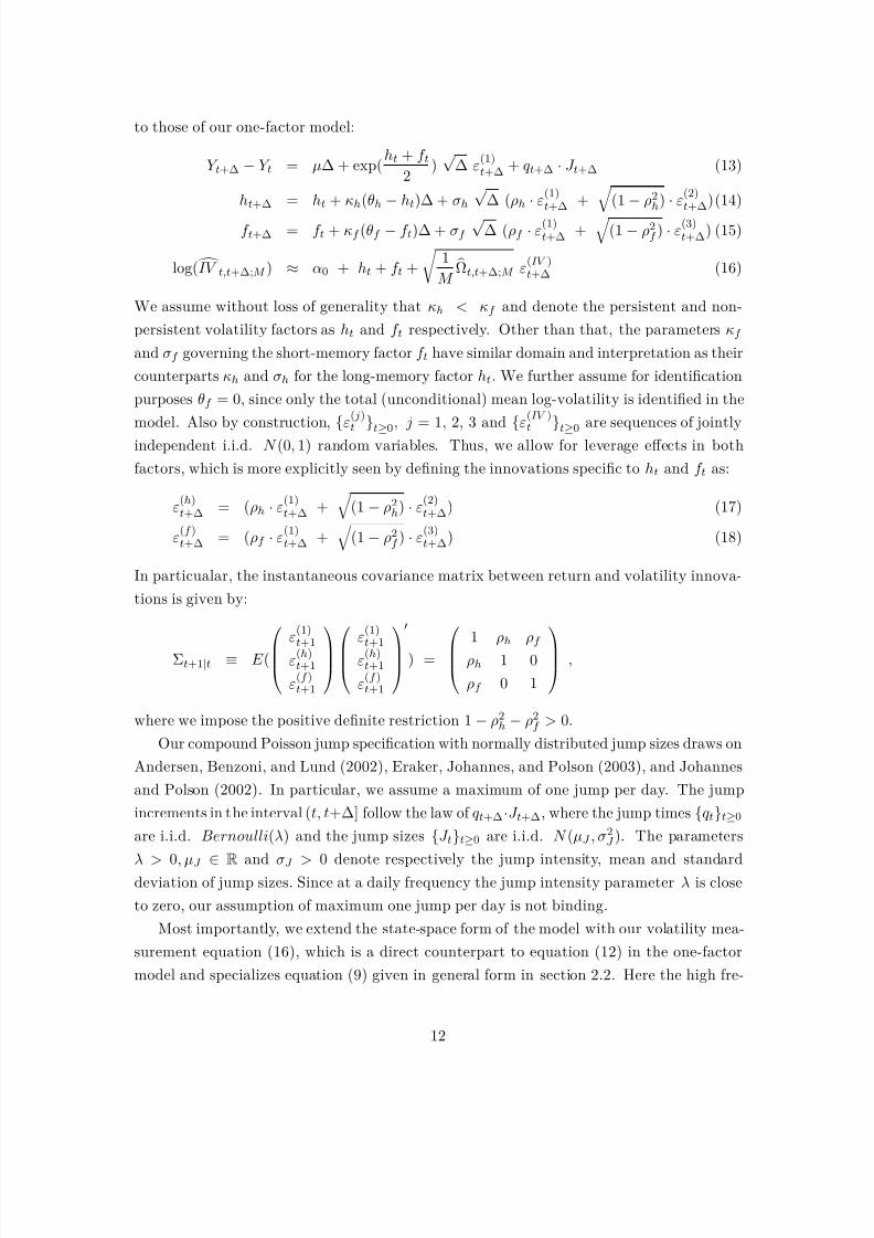
to those of our one-factor model:
Y t+∆ − Y t = µ∆ + exp(ht + f t
2)√
∆ ε(1)t+∆ + qt+∆ · J t+∆ (13)
ht+∆ = ht + κh(θh−
ht)∆ + σh√
∆ (ρh·
ε(1)t+∆ + (1
−ρ2h)
·ε(2)t+∆)(14)
f t+∆ = f t + κf (θf − f t)∆ + σf √
∆ (ρf · ε(1)t+∆ +
(1 − ρ2f ) · ε
(3)t+∆) (15)
log(IV t,t+∆;M ) ≈ α0 + ht + f t +
1
M Ωt,t+∆;M ε
(IV )t+∆ (16)
We assume without loss of generality that κh < κf and denote the persistent and non-
persistent volatility factors as ht and f t respectively. Other than that, the parameters κf
and σf governing the short-memory factor f t have similar domain and interpretation as their
counterparts κh and σh for the long-memory factor ht. We further assume for identification
purposes θf = 0, since only the total (unconditional) mean log-volatility is identified in the
model. Also by construction, ε
( j)
t t≥0, j = 1, 2, 3 and ε
(IV )
t t≥0 are sequences of jointlyindependent i.i.d. N (0, 1) random variables. Thus, we allow for leverage effects in both
factors, which is more explicitly seen by defining the innovations specific to ht and f t as:
ε(h)t+∆ = (ρh · ε
(1)t+∆ +
(1 − ρ2h) · ε
(2)t+∆) (17)
ε(f )t+∆ = (ρf · ε
(1)t+∆ +
(1 − ρ2f ) · ε
(3)t+∆) (18)
In particualar, the instantaneous covariance matrix between return and volatility innova-
tions is given by:
Σt+1|t ≡ E ( ε
(1)
t+1ε(h)t+1
ε(f )t+1
ε
(1)
t+1ε(h)t+1
ε(f )t+1
) = 1 ρh ρf
ρh 1 0
ρf 0 1
,
where we impose the positive definite restriction 1 − ρ2h − ρ2f > 0.
Our compound Poisson jump specification with normally distributed jump sizes draws on
Andersen, Benzoni, and Lund (2002), Eraker, Johannes, and Polson (2003), and Johannes
and Polson (2002). In particular, we assume a maximum of one jump per day. The jump
increments in the interval (t, t+∆] follow the law of qt+∆·J t+∆, where the jump times qtt≥0are i.i.d. Bernoulli(λ) and the jump sizes J tt≥0 are i.i.d. N (µJ , σ2
J ). The parameters
λ > 0, µJ ∈ R and σJ > 0 denote respectively the jump intensity, mean and standarddeviation of jump sizes. Since at a daily frequency the jump intensity parameter λ is close
to zero, our assumption of maximum one jump per day is not binding.
Most importantly, we extend the state-space form of the model with our volatility mea-
surement equation (16), which is a direct counterpart to equation (12) in the one-factor
model and specializes equation (9) given in general form in section 2.2. Here the high fre-
12
8/3/2019 The In Format In Content of High-Frequency Data for Estimating Equity Return Models
http://slidepdf.com/reader/full/the-in-format-in-content-of-high-frequency-data-for-estimating-equity-return 18/48
quency measure of log integrated variance log(IV t,t+∆;M ) is an estimate of ht + f t as the
total diffusive variance in the two-factor model. The extra parameter α0 serves the same
purpose as in the one-factor model. It provides standard correction for the discrepancy
between log integrated variance measures log(IV t,t+∆;M ) calculated using open-to-close in-
traday data and the log variance of close-to-close daily returns modeled by ht + f t. For
modeling the log variance of open-to-close daily returns we simply restrict α0 = 0.
In order to find the contribution of high frequency information, similarly to our one-
factor model, we consider two versions of the two factor model: (i) the one with only
daily returns; (ii) the one including both daily returns and a daily volatility measurement
equation from high frequency intraday data. The former is given by the system of equations
(13)-(15), while the latter consists of all equations from the “daily” model augmented by
our additional volatility measurement equation (16).
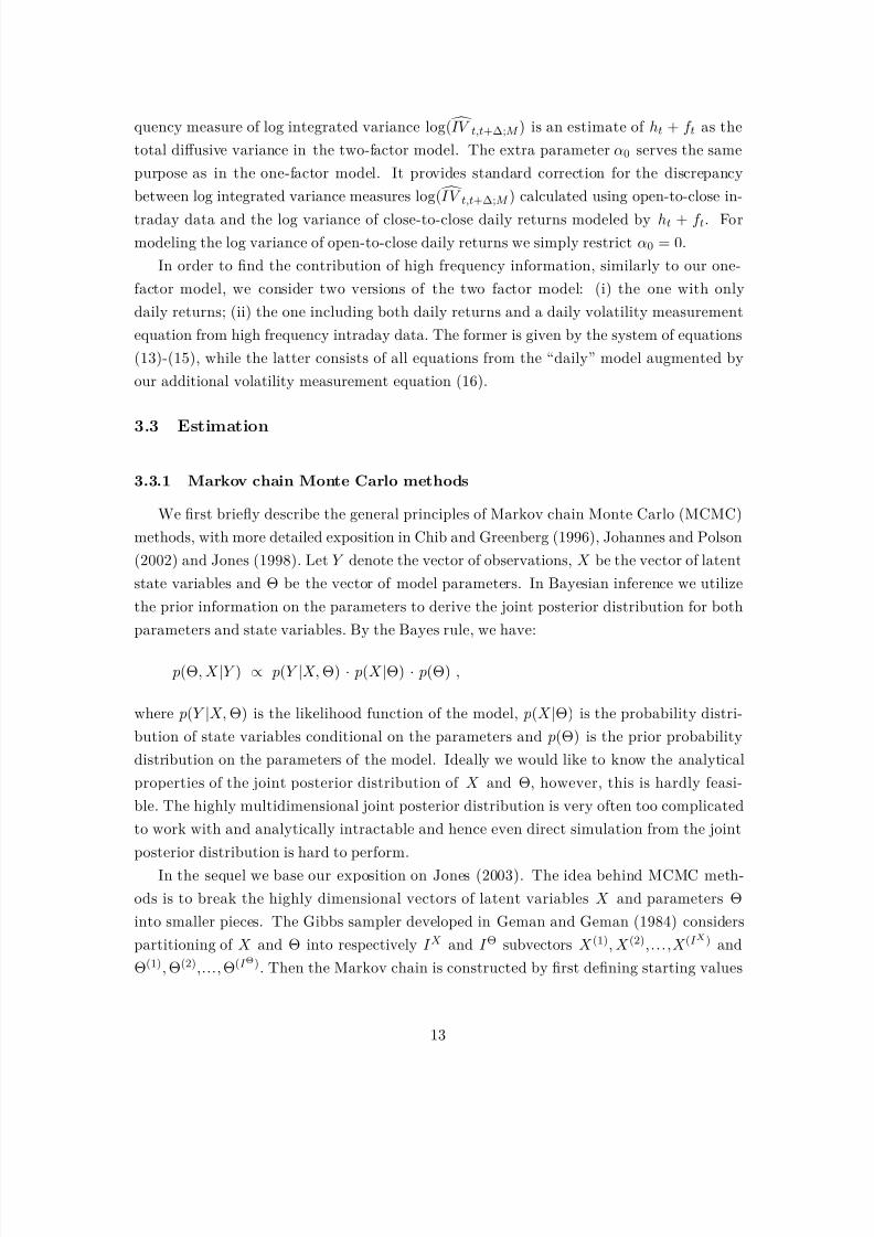
3.3 Estimation
3.3.1 Markov chain Monte Carlo methods
We first briefly describe the general principles of Markov chain Monte Carlo (MCMC)
methods, with more detailed exposition in Chib and Greenberg (1996), Johannes and Polson
(2002) and Jones (1998). Let Y denote the vector of observations, X be the vector of latent
state variables and Θ be the vector of model parameters. In Bayesian inference we utilize
the prior information on the parameters to derive the joint posterior distribution for both
parameters and state variables. By the Bayes rule, we have:
p(Θ, X |Y ) ∝ p(Y |X, Θ) · p(X |Θ) · p(Θ) ,
where p(Y |X, Θ) is the likelihood function of the model, p(X |Θ) is the probability distri-
bution of state variables conditional on the parameters and p(Θ) is the prior probability
distribution on the parameters of the model. Ideally we would like to know the analytical
properties of the joint posterior distribution of X and Θ, however, this is hardly feasi-
ble. The highly multidimensional joint posterior distribution is very often too complicated
to work with and analytically intractable and hence even direct simulation from the joint
posterior distribution is hard to perform.In the sequel we base our exposition on Jones (2003). The idea behind MCMC meth-
ods is to break the highly dimensional vectors of latent variables X and parameters Θ
into smaller pieces. The Gibbs sampler developed in Geman and Geman (1984) considers
partitioning of X and Θ into respectively I X and I Θ subvectors X (1), X (2),...,X (I X) and
Θ(1), Θ(2),..., Θ(I Θ). Then the Markov chain is constructed by first defining starting values
13
8/3/2019 The In Format In Content of High-Frequency Data for Estimating Equity Return Models
http://slidepdf.com/reader/full/the-in-format-in-content-of-high-frequency-data-for-estimating-equity-return 19/48
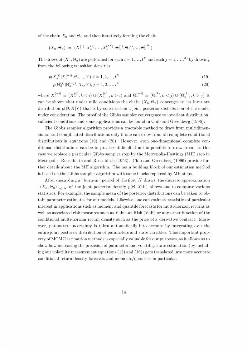
of the chain X 0 and Θ0 and then iteratively forming the chain
(X n, Θn) = (X (1)n , X (2)n ,...,X (I X)
n , Θ(1)n , Θ(2)
n ,..., Θ(I Θ)n )
The draws of (X n, Θn) are performed for each i = 1,...,I X
and each j = 1,...,I Θ
by drawingfrom the following transition densities:
p(X (i)n |X (−i)n , Θn−1, Y ), i = 1, 2,...,I X (19)
p(Θ( j)n |Θ(− j)
n , X n, Y ), j = 1, 2,...,I Θ (20)
where X (−i)n ≡ (X
(k)n ; k < i) ∪ (X
(k)n−1; k > i) and Θ
(− j)n ≡ (Θ
(k)n ; k < j) ∪ (Θ
(k)n−1; k > j) It
can be shown that under mild conditions the chain (X n, Θn) converges to its invariant
distribution p(Θ, X |Y ) that is by construction a joint posterior distribution of the model
under consideration. The proof of the Gibbs sampler convergence to invariant distribution,
sufficient conditions and some applications can be found in Chib and Greenberg (1996).The Gibbs sampler algorithm provides a tractable method to draw from multidimen-
sional and complicated distributions only if one can draw from all complete conditional
distributions in equations (19) and (20). However, even one-dimensional complete con-
ditional distributions can be in practice difficult if not impossible to draw from. In this
case we replace a particular Gibbs sampler step by the Metropolis-Hastings (MH) step in
Metropolis, Rosenbluth and Rosenbluth (1953). Chib and Greenberg (1996) provide fur-
ther details about the MH algorithm. The main building block of our estimation method
is based on the Gibbs sampler algorithm with some blocks replaced by MH steps.
After discarding a “burn-in” period of the first N draws, the discrete approximation(X n, Θn)n>N of the joint posterior density p(Θ, X |Y ) allows one to compute various
statistics. For example, the sample mean of the posterior distributions can be taken to ob-
tain parameter estimates for our models. Likewise, one can estimate statistics of particular
interest in applications such as moment and quantile forecasts for multi-horizon returns as
well as associated risk measures such as Value-at-Risk (VaR) or any other function of the
conditional multi-horizon return density such as the price of a derivative contract. More-
over, parameter uncertainty is taken automatically into account by integrating over the
entire joint posterior distribution of parameters and state variables. This important prop-
erty of MCMC estimation methods is especially valuable for our purposes, as it allows us to
show how increasing the precision of parameter and volatility state estimation (by includ-
ing our volatility measurement equations (12) and (16)) gets translated into more accurate
conditional return density forecasts and moments/quantiles in particular.
14
8/3/2019 The In Format In Content of High-Frequency Data for Estimating Equity Return Models
http://slidepdf.com/reader/full/the-in-format-in-content-of-high-frequency-data-for-estimating-equity-return 20/48
3.3.2 Bayesian MCMC inference for models with high frequency volatility
measurement equations
We limit our exposition to describing our MCMC estimation procedure for the two-
factor stochastic volatility models from Section (3.2).19 We put special emphasis on how to
estimate models including our high-frequency measurement equations by offering a straight-
forward extension of estimation methods based only on daily returns.
Following the notation from the previous section, we need to specify the vector of obser-
vations Y , the vector of latent state variables X and the vector of parameters Θ along with
their appropriate subdivision in line with the construction of the Gibbs sampler algorithm.
In particular, we define the following vectors, where “Daily” stays for estimation based only
on daily returns (equations (13)-(15)) and “HF” stays for estimation incorporating also
volatility measures based on high-frequency intraday data (equations (13)-(16)):
Y (Daily) = Y tt=1,...,T Y (HF ) = Y tt=1,...,T , IV t,t+1;M t=1,...,T −1, Ωt,t+1;M t=1,...,T −1
X = htt=1,...,T , f tt=1,...,T , qtt=2,...,T , J tt=2,...,T Θ = µ, κh, θh, (σh, ρh), κf , (σf , ρf ), λ , µJ , σJ , α0 .
The partitions of Θ and X are given by Θ(1) = µ, Θ(2) = κh, Θ(3) = θh, Θ(4) = (σh, ρh),
Θ(5) = κf , Θ(6) = (σf , ρf ), Θ(7) = λ, Θ(8) = µJ , Θ(9) = σJ and X (i) = hi, X (i+T ) = f i,
X ( j+2T ) = q j+1, X ( j+(3T −1)) = J j+1 where i = 1, 2,...,T , j = 1,...,T − 1. Thus, we treat
each element of the state vector X as a single block. For the vector of parameters Θ allelements are treated as a single block with the exception of (σh, ρh) and (σf , ρf ). These
parameters are drawn jointly as in Jacquier, Polson, and Rossi (2004). Finally, the extra
parameter Θ(10) = α0 in equation (16) appears only in the “HF” model including high
frequency information and is estimated along with the rest of the parameters or it can be
exogenously specified following standard approaches in the realized volatility literature to
obtain variances for the whole day such as Hansen and Lunde (2005). It is set to zero when
modeling open-to-close daily returns.
Having defined above all blocks for the latent state variables X and parameters Θ, we
apply the MCMC algorithm based on the Gibbs sampler presented in Section 3.3.1. Sincedraws of all parameters and jump related latent variables are standard in the literature, we
directly refer to Szerszen (2009) for the imposed prior distributions on the model parameters
Θ and all other details.
Here we focus on addressing the fundamental difference between estimation of the stan-
19One-factor models can be viewed as a special case by restricting f t = 0 for all t, omitting the parametersκf , θf , σf , ρf for the f factor and imposing the constraint ρf = 0 in the instantaneous correlation matrix.
15
8/3/2019 The In Format In Content of High-Frequency Data for Estimating Equity Return Models
http://slidepdf.com/reader/full/the-in-format-in-content-of-high-frequency-data-for-estimating-equity-return 21/48
dard “Daily” and our “HF” version of the model, which differ just by the additional volatility
measurement equation (16) based on high-frequency data. The information provided by this
extra equation affects only the complete conditional posteriors of the volatility states ht and
f t. In particular, the MCMC update for ht is given by
p(ht|f t, ht+1, ht−1,q,J, Θ, Y ) ∝ p(Y t+1|Y t, f t, ht, Θ, q , J ) · p(Y t|Y t−1, f t, ht, Θ, q , J )
· p(ht+1|ht, Θ) · p(ht|ht−1, Θ) · p(ht|IV t,t+1;M , Ωt,t+1;M , f t, Θ)
for t=1, 2, ..., T, where the second and fourth kernels on the right hand side are omitted
for t=1, while the first, third and last kernels are omitted for t=T. The MCMC update for
the second factor f t is performed analogously.
Thus, an inspection of the above update expression reveals that the only kernel affected
by the high frequency information with Y = Y (HF ) is the last one p(ht|
IV t,t+1;M ,
Ωt,t+1;M , f t)
for the h factor and, similarly, p(f t|IV t,t+1;M , Ωt,t+1;M , ht) for the f factor. The rest of the
kernels are exactly those coming from inference based on daily returns only, i.e. with Y =
Y (Daily), which appear also with Y = Y (HF ). This is of key importance for understanding
how the extra information provided by high-frequency data improves estimation efficiency
in our “HF” versus “Daily” approaches. The extra kernels p(ht|IV t,t+1;M , Ωt,t+1;M , f t) and
p(f t|IV t,t+1;M , Ωt,t+1;M , ht) in the MCMC updates of h and f , respectively, are very spiked
around the mode for dates with low values of 1M Ωt,t+1;M in the volatility measurement
equation (16) and, hence, they are very informative about the latent volatility states. The
attainable precision improvements increase with the sample frequency M and depend also on
Ωt,t+1;M , being a function of the underlying volatility paths and the chosen high-frequency
integrated variance and quarticity measures as detailed in Section 2.2. By contrast, theuse of only daily data is equivalent to artificially setting 1
M Ωt,t+1;M to infinity in order to
suppress the strong information content of high frequency data provided by our volatility
measurement equation. In what follows, we analyze the gains in estimation efficiency and
risk forecasting accuracy from our “HF” versus traditional “Daily” estimation as a natural
benchmark for comparison.
4 Estimation efficiency and risk forecasting accuracy
The ability to estimate parameters and volatility states more efficiently directly trans-lates into more accurate risk forecasts. Moreover, the highly non-linear nature of the under-
lying transformation from noisy parameter and volatility estimates to risk forecasts implies
reduction not only in the variance but also in the bias of the prediction errors. Our analysis
in this section is designed to study the interplay between longer sample size and higher
intraday frequency as an additional source of information introduced by our volatility mea-
surement equation for the purpose of reducing estimation uncertainty. We document that
16
8/3/2019 The In Format In Content of High-Frequency Data for Estimating Equity Return Models
http://slidepdf.com/reader/full/the-in-format-in-content-of-high-frequency-data-for-estimating-equity-return 22/48
even for the longest sample lengths encountered in practice there is a substantial efficiency
gain from incorporating the extra information provided by high-frequency volatility mea-
sures. Moreover, for key model parameters controlling skewness and kurtosis we find that
two or five years of high frequency data would suffice to obtain the same level of precision
as twenty years of daily data. This suggests that our approach can be particularly useful in
finance applications where only short data samples are available or economically meaningful
to use.
It is possible to derive analytical results along these lines in certain more restrictive
settings. An instructive example for a canonical log-SV model is given in the appendix.
Monte Carlo analysis is the only viable option, though, for models that are not analyti-
cally tractable. Hence, we take a Monte Carlo approach to study estimation efficiency and
the impact of parameter uncertainty on risk forecasting accuracy. We conduct considerably
more thorough and extensive simulations than usual in order to properly document the sub-
stantial efficiency gains and improved precision of risk forecasts at horizons of up to a fewmonths ahead regardless of the chosen model when high frequency information is included
in the model. Perhaps the most important of our findings is that there is considerable
asymmetry between bad and good times when it comes to the attainable improvements in
risk forecasting accuracy: in good times we are able to largely eliminate overstatement of
risk, while in bad times our approach helps avoid understatement of risk. From a practical
point of view, this implies imposing an appropriate larger risk cushion exactly when needed
the most, e.g. early on in times of crisis (rather than with a delay), while at the same
time avoiding excessive risk cushion requirements in normal times. In this sense, our main
purpose in what follows is to document both the efficiency gains for model estimation and
forecasting and the implied potentially large economic value of our approach to incorporat-
ing the information content of high-frequency volatility measures for model estimation and
risk forecasting.
4.1 Monte Carlo setup
In order to set-up the stage for Monte Carlo analysis we first describe how to draw sam-
ple paths consistent with the data generating process implied by our model specifications.
Daily dynamics of both returns and volatility are based on equations (10)-(11) and (13)-(15)
respectively for the one-factor and two-factor log-SV models that we consider. The intradaydynamics is based on a Brownian bridge connecting consecutive daily sample points and
producing valid integrated variance measures IV t,t+1;M t≥0 and corresponding scaled inte-
grated quarticity measures Ωt,t+1;M t≥0 that govern our additional volatility measurement
equations in (12) and (16) as described in Section 2.2. In this way, we allow for poten-
tially richer intraday dynamics than the one at the daily frequency, possibly including also
realistic intraday market-microstructure effects that many novel high-frequency volatility
17
8/3/2019 The In Format In Content of High-Frequency Data for Estimating Equity Return Models
http://slidepdf.com/reader/full/the-in-format-in-content-of-high-frequency-data-for-estimating-equity-return 23/48
measures are designed to be robust to when sampled at two to five minute frequency.20
We draw 1,000 sample paths for each of the considered one- and two-factor log-SV
models. For each sample path we estimate the underlying model parameters using different
information sets: (i) daily data only; (ii) daily data with additional high frequency volatility
measurements based on 5-minute or 2-minute intraday returns; (iii) the “infeasible” case of
perfectly observed volatility.21 In order to study the interplay between additional informa-
tion coming from more high frequency data and longer sample size in terms of number of
days, we consider three sample windows of 2, 5 and 20 years. This gives a total of twelve
one-factor and twelve two-factor specifications for the information sets used for model es-
timation. We estimate all specifications using the Bayesian MCMC methods described in
Section 3 with 250,000 draws, where the first 50,000 draws are discarded as the burn-in
sample. For the purposes of forecasting conditional return moments and quantiles, based
on the obtained 200,000 draws of the posterior distribution of parameters and volatility
states, we approximate multi-period conditional density forecasts by a cloud of 25,000,000points. We then compare moments and quantiles of the obtained conditional density fore-
casts for the two different estimation procedures that we consider, depending on whether a
daily volatility measurement equation based on high-frequency data is used or not.
4.2 Efficiency gains in parameter and volatility estimation
In Tables 1 and 2 we report parameter estimates, bias and root mean squared error
(RMSE) of volatility related parameters governing equations (11) and (14)-(15) for our
one-factor and two-factor specifications respectively. The true parameter values in each
table represent our estimates on S&P 500 daily futures returns for the period October 2,1985 - February 26, 2009.
For the one-factor model (Table 1) we attain up to few times better precision when
using high frequency data compared to only daily data for estimating the parameters gov-
erning skewness and kurtosis. This translates into RMSE reduction of as much as 70%.
In particular, we find that the information content of high-frequency volatility measures
improves the most the estimation efficiency of the volatility of volatility parameter σh and
the leverage effect parameter ρh in the model.22 Moreover, the gains are consistent across
different sample lengths, even for the longest ones typically encountered in practice such as
20
In particular, in our analysis we focus on the MedRV estimator of Andersen, Dobrev, and Schaumburg(2009) and the tri-power variation measure of Barndorff-Nielsen, Shephard, and Winkel (2006). We reportresults only for the former as the results obtained for the latter are in the same spirit.
21In the one-factor model the case of perfectly observed volatility can be viewed as the limiting case of our volatility measurement equation when the intraday sample frequency grows to infinity. In the two-factormodel, though, the volatility measurement equation provides information only about the sum of the twovolatility factors without separating them as in the infeasible case of full observability.
22In this sense, our results extend those obtained by Alizadeh, Brandt, and Diebold (2002) in a considerablymore restrictive range-based analysis of a model without leverage effects.
18
8/3/2019 The In Format In Content of High-Frequency Data for Estimating Equity Return Models
http://slidepdf.com/reader/full/the-in-format-in-content-of-high-frequency-data-for-estimating-equity-return 24/48
20 years, when daily estimation is more likely to produce satisfactory results. As a practical
rule of thumb we find that two years of high frequency data often suffice to obtain the same
level of precision for these parameters as twenty years of daily data. At the same time, a
comparison between the attainable improvement by switching from daily to 5-minute esti-
mation and any further increase in the intraday sample frequency from 5 to 2 minutes and
beyond (up to the infeasible case of perfectly known volatility) reveals a rapid decrease in
the additional efficiency gains that can be obtained. We also observe a substantial RMSE
reduction for the parameter governing persistence of volatility κh for the shortest sample
sizes, while still dominating the estimation efficiency with only daily data across all sample
sizes.
For the richer two-factor log-SV model (Table 2) these substantial efficiency gains from
incorporating high-frequency volatility measures naturally get even larger. Moreover, a
somewhat larger part of the gains is due to bias reduction. It is important to note that
here skewness and kurtosis are driven not only by a persistent volatility factor but also bya second non-persistent factor. For the non-persistent factor we find that the gains from
incorporating high frequency information are more pronounced than those from increasing
the yearly sample length. We do not find such evidence for the persistent factor, where
both sources of information play an important role in parameter estimation. This implies
bigger efficiency gains from incorporating high frequency information for the parameters
ρf and σf governing skewness and kurtosis arising from the non-persistent factor f . The
reduction of parameter uncertainty for the persistent factor h is somewhat smaller but still
very visible.
The quality of risk forecasts depends not only on the degree of parameter uncertainty
but also on the degree of volatility estimation uncertainty. In particular, it is important to
assess the impact of incorporating additional high frequency information on the accuracy
of estimation of terminal volatility states as they play important role in forecasting risk.
In Table 3 we report mean estimates, bias and RMSE for the terminal volatility states hT
and f T of the two-factor log-SV model. Thus, we conclude that our volatility measurement
equation helps in estimating better not only model parameters but also latent volatility
states. Considerable efficiency gains are obtained mainly for the persistent volatility factor,
while for the non-persistent factor we still observe slight improvements. Similarly to param-
eter estimates, our findings for volatility states are consistent across all considered sample
sizes. Moreover, the biggest efficiency gains take place when moving from estimation based
only on daily data to estimation incorporating our volatility measurement equation based
on 5-minute returns. Further increase of the intraday sample frequency from 5-minutes
to 2-minutes leads to additional efficiency gains of much smaller magnitude. Overall, for
the estimation of volatility states adding high frequency information has somewhat bigger
importance than increasing the yearly sample length. This plays a major role especially for
19
8/3/2019 The In Format In Content of High-Frequency Data for Estimating Equity Return Models
http://slidepdf.com/reader/full/the-in-format-in-content-of-high-frequency-data-for-estimating-equity-return 25/48
short-term risk forecasting.
4.3 Precision improvements in risk forecasting accuracy
The documented substantial decrease in parameter and volatility estimation uncertainty
implies non-trivial improvements in the accuracy of forecasts of conditional return moments
and quantiles. We compare forecasts resulting from inference based on daily data to those
utilizing 5-minute high frequency volatility measures. We restrict attention to the 5-minute
frequency in accordance with our finding that it offers essentially the bulk of the attainable
improvements based on our volatility measurement equation. We perform our analysis in-
corporating parameter and volatility estimation uncertainty for all three considered sample
lengths of 2, 5 and 20 years.
In Tables 4 and 5 we report forecasts of conditional return moments respectively for
one-factor and two-factor models. In Tables 6 and 7 we also report forecasts of conditional
return quantiles. The considered forecast horizons are 1, 5, 10 and 20 days ahead and are
presented in separate panels in each table. These forecast horizons are of primary interest
in many finance applications.
Our main finding is that our more efficient parameter and state estimates incorporating
the strong information content of high-frequency volatility measures translate into equally
better conditional return density forecasts not only in terms of RMSE but also in terms
of bias. The bias reduction is due to the pronounced non-linearities in the underlying
transformation of parameters and state variables. The main message from our analysis
summarized in Tables 4-7 is that for any model, any estimation sample length, and across
all forecast horizons of interest, the forecasts incorporating the extra information from ourvolatility measurement equation clearly dominate those based only on daily data. Moreover,
these results strengthen our rule of thumb that model specifications estimated with two years
of high frequency data perform at least as good as the same model specifications estimated
with twenty years of daily data, which in turn are considerably outperformed if estimated
on twenty years of high-frequency data.
4.4 Forecast error reductions in good versus bad times
From risk management perspective it is important to know how the improvements in
risk forecasting accuracy vary across good and bad times. To this end, in Table 8 we reportrelative errors of forecasts of the 0.01 and 0.05 conditional return quantiles at horizons
of one (panel A), five (panel B), ten (panel C) and twenty (panel D) days ahead. The
reported relative errors are calculated across 1,000 Monte Carlo replications as the mean of
the percentage difference between a forecast based on parameter and state estimates and
the forecast based on the corresponding true values. The results are sorted by the rank
20
8/3/2019 The In Format In Content of High-Frequency Data for Estimating Equity Return Models
http://slidepdf.com/reader/full/the-in-format-in-content-of-high-frequency-data-for-estimating-equity-return 26/48
order of the true quantile forecasts from low (representing bad times) to high (representing
good times), as indicated in the first column. In our model this is equivalent to sorting by
terminal volatility state from high (representing bad times) to low (representing good times).
Each three rows reported for ranks 1 (low) to 5 (high) of the true quantile forecasts contain
results for three different sample lengths T equal to 2 years, 5 years and 20 years (as given
in the second column), taking parameter and volatility estimation uncertainty into account.
For each quantile and forecast horizon we report results for the two alternative Bayesian
estimation procedures in adjacent column pairs: either with (right column denoted “HF
5-min”) or without (left column denoted “Daily only”) augmenting the underlying state-
space formulation with our daily volatility measurement equation based on high frequency
intraday data.
As a graphical summary of the results reported in Table 8, Figure 1 plots the one-percent
VaR (top graph) and five-percent VaR (bottom graph) relative forecast errors at a five-day
horizon as a function of the rank order of the underlying true forecasts from low (repre-senting bad times) to high (representing good times). The resulting VaR forecast errors
without utilizing our high-frequency volatility measures are plotted as a solid line (denoted
“Daily”), while those incorporating the information content of intraday data for the latent
daily volatility are plotted as a dashed line (denoted “HF 5-min”). The reported relative
errors of conditional return quantile forecasts can be interpreted also as the percentage
overestimation or understimation of the implied capital charge for market risk based on
one-percent (quantile 0.01) and five-percent (quantile 0.05) VaR.
Both Table 8 and Figure 1 reveal that risk forecasts stemming from traditional model
inference on daily data tend to be overly conservative in good times (e.g. overestimating risk
by as much as 30%) but they are not conservative enough in bad times (e.g. underestimating
risk by as much as 10%). By contrast, risk forecasts based on our approach to exploiting
high-frequency data are considerably closer to the truth in both bad and good times.
Leaving the reported magnitudes aside, this result is very intuitive as the use of volatility
measures based on high frequency data allows for considerably faster and more precise
incorporation of major changes in the current volatility level compared to daily data alone.
For example, in bad times when volatility goes up it should take a longer sequence of
daily returns alone than in conjunction with high-frequency volatility measures to deliver
volatility state estimates that are not downward biased. Similarly, in good times when
volatility goes down it should take longer for daily data alone than in conjunction with
high-frequency volatility measures to produce volatility state estimates that are not upward
biased. Thus, the observed differences between the risk forecast errors in bad versus good
times (Table 8 and Figure 1) are completely in line with the asymmetric increase in volatility
state uncertainty, coupled also with higher parameter uncertainty (see Section 4.2 above),
characterizing traditional daily estimation in comparison to the proposed approach utilizing
21
8/3/2019 The In Format In Content of High-Frequency Data for Estimating Equity Return Models
http://slidepdf.com/reader/full/the-in-format-in-content-of-high-frequency-data-for-estimating-equity-return 27/48
also high-frequency data. In sum, thanks to incorporating the strong information content
of high-frequency volatility measures, we are able to better curb risk taking exactly when
needed the most, i.e. early on in times of crisis, while avoiding unnecessary overstatement
of risk in normal times.
5 Empirical Illustration
Conditional return quantile forecasts play important role in risk management as they
represent value-at-risk (VaR) forecasts. A key testable implication from our analysis in the
previous section is that during bad times, e.g. early on in times of crisis, VaR forecast time-
series based on our approach to exploiting high-frequency data will tend to “cross from
above” the VaR forecast time-series stemming from traditional model inference on daily
data. This is because, as explained above, the daily-based VaR forecasts are downward
biased in bad times (when risk is elevated) and upward biased in good times (when risk isminimal), while our HF-based VaR forecasts are considerably closer to the truth in both
bad and good times.
In order to test the empirical validity of this important risk management implication,
we study the dynamics of five-day ahead VaR forecasts for S&P 500 and Google returns
throughout the financial crisis of 2007-2008. Our goal is to illustrate the potentially large
economic value from the proposed approach to incorporating the information content of
high-frequency volatility measures. It is beyond the scope of this paper, though, to run a
horse race between many viable alternative VaR forecasting techniques. We limit ourselves
strictly to evaluating the empirical validity of our main testable implication with regard to
HF-based versus daily-based VaR forecasts in the context of popular equity return models
such as the fairly general two-factor log-SV model with jumps analyzed in the previous
sections.
5.1 Data and estimation
In our empirical illustration we consider S&P 500 daily futures returns for the period
October 2, 1985 - February 26, 2009 and Google daily equity returns for the period August
30, 2004 - July 31, 2009.23 We exclude from each series holidays and shortened trading
days. Our high-frequency measurement equation is constructed from five-minute intradayreturns following the procedures given in section 2.2, while model estimation and forecasting
is conducted as detailed in sections 3 and 4. We study the dynamics of five-day ahead VaR
forecasts for the last 120 business weeks in each sample, both of which cover the financial
crisis of 2007-2008. To produce each forecast we re-estimate our two-factor log-SV model
23The data for S&P 500 is provided by Tick Data, while the data for Google is from NYSE TAQ.
22
8/3/2019 The In Format In Content of High-Frequency Data for Estimating Equity Return Models
http://slidepdf.com/reader/full/the-in-format-in-content-of-high-frequency-data-for-estimating-equity-return 28/48
with all available data going back to the beginning of each sample. Thus, the sample for
S&P 500 roughly corresponds to 20 years of data in our Monte Carlo study (Section 4). The
sample for Google, on the other hand, represents 2-5 years of data and cannot be extended
further back as it starts ten days after Google’s IPO.
5.2 Forecasting risk throughout the 2007-2008 financial crisis
On Figures 2 and 3 we plot one-percent (top graph) and five-percent (bottom graph)
VaR forecasts without overlapping at five-day horizon for S&P 500 futures returns (Figure
2) and Google equity returns (Figure 3) based on a two-factor log-SV model with jumps
in returns. The model is estimated at a daily discretization interval by Bayesian MCMC
methods either without or with augmenting the underlying state-space formulation with our
daily volatility measurement equation based on high frequency intraday data. The resulting
VaR forecasts without utilizing high-frequency volatility measures are plotted as a solid line
(denoted “VaR with daily data”), those incorporating the information content of intraday
data for the latent daily volatility are plotted as a dashed line (denoted “VaR with HF
5-min data”), while the corresponding actual observed returns are plotted as vertical bars
(denoted “Return realizations”).
As clearly seen from the graphs, the VaR forecasts with HF 5-min data seemingly
correctly predict more risk and “cross from above” the VaR forecasts with daily data exactly
around major turmoil events during the financial crisis of 2007-2008. These include the Bear
Sterns turmoil in July 2007, the Countrywide turmoil in January 2008, the Fannie Mae and
Freddie Mac turmoil in July 2008, and most notably, the Lehman Brothers collapse followed
by the TARP Legislation turmoil in October 2008. The gap between the two alternativeVaR forecasts around these events implies sizeable underestimation of risk by the traditional
approach based on daily data. This is more pronounced for Google in line with the fact that
individual stocks tend to be more risky than stock indices. At the same time, before the
summer of 2007 and on many occasions afterwards the VaR forecasts with HF 5-min data
predict a bit less risk than the VaR forecasts with daily data. Nonetheless, the number of
incurred violations (given by the number of times the return realizations, plotted as vertical
bars, go below the VaR forecasts) remains completely in line with the expected number of
violations at the 1% and 5% VaR levels across 120 (non-overlapping) forecasts.
Overall, the observed dynamics of VaR forecasts for S&P 500 and Google returnsthroughout the financial crisis of 2007-2008 is in striking agreement with the key testable
implication from our analysis in the previous sections. We obtain strong empirical support
that not only in theory but also in important real-world examples our approach to incorpo-
rating the information content of high frequency volatility measures can help better curb
risk taking exactly when needed the most, i.e. early on in times of crisis, while avoiding
unnecessary overstatement of risk in normal times.
23
8/3/2019 The In Format In Content of High-Frequency Data for Estimating Equity Return Models
http://slidepdf.com/reader/full/the-in-format-in-content-of-high-frequency-data-for-estimating-equity-return 29/48
6 Conclusion
In this paper, we have developed a method for estimating popular equity return models
relying not only on daily returns but also on nowadays ubiquitous high-frequency intraday
return data. The essence of our approach is to borrow asymptotic results from the grow-ing realized volatility literature and cast them as precise volatility measurement equations
directly within the standard state-space representation of popular equity return models
estimated at daily frequency. In this way, we avoid specifying explicitly the intraday re-
turn dynamics, while considerably improving estimation efficiency of such models at daily
or monthly frequency. In particular, we utilize daily returns along with high-frequency
jump-robust realized volatility measures within a standard Bayesian MCMC estimation
framework. This allows us to take explicitly into account the resulting substantial reduc-
tion in parameter uncertainty. Thus, we are able to show sizeable economic gains when
forecasting risk, compared to inference based on the more limited information provided by
daily returns alone.
In this way, we depart from previous studies geared primarily towards specification
testing that have focused on the use of such high-frequency volatility measures in classi-
cal rather than Bayesian estimation procedures. Instead, we demonstrate that across a
variety of equity return models estimated at daily frequency the parameters controlling
skewness and kurtosis can be obtained almost as precisely as if volatility is observable
by incorporating the strong information content of realized volatility measures extracted
from high-frequency data. In particular, we show that not only the parameters controlling
volatility of volatility but also those controlling leverage effects can be estimated several
times more precisely by exploiting high-frequency volatility measures. Furthermore, we
show that our highly efficient estimates lead in turn to substantial gains for forecasting
various risk measures at horizons ranging from a few days to a few months ahead when
taking also into account parameter uncertainty. In fact, our approach not only reduces the
root mean square prediction error but also shrinks and almost eliminates the forecast bias,
which inevitably arises from the pronounced nonlinearities in the involved transformation
of parameter and volatility estimates. As a practical rule of thumb we find that two years
of high frequency data often suffice to obtain the same level of precision as twenty years of
daily data, thereby making our approach particularly useful in finance applications where
only short data samples are available or economically meaningful to use. Last, but perhapsmost important in risk management applications, we find that risk forecasts based on our
approach to exploiting high-frequency data are considerably closer to the truth in both bad
and good times relative to those stemming from traditional model inference on daily data,
which we find can overestimate risk by as much as 30% in good times or underestimate
it by as much as 10% in bad times. We support our findings both with extensive simula-
24
8/3/2019 The In Format In Content of High-Frequency Data for Estimating Equity Return Models
http://slidepdf.com/reader/full/the-in-format-in-content-of-high-frequency-data-for-estimating-equity-return 30/48
tions and an empirical illustration on VaR forecasts for S&P500 and Google returns during
the financial crisis of 2007-2008. Thanks to incorporating the strong information content
of high-frequency volatility measures, we are able to better curb risk taking exactly when
needed the most, i.e. early on in times of crisis (rather than with a delay), while avoiding
unnecessary overstatement of risk in normal times. Qualitatively, our findings are robust
both across different models and jump-robust volatility measures on high frequency data
that we analyze.
In view of the documented substantial precision gains in forecasting risk of equity re-
turns, the estimation approach we propose can directly add value in different areas of risk
management and asset pricing. Beyond equity returns, the method can be applied also to
other financial data such as foreign exchange rates, bonds and interest rates. It can be easily
geared also towards model specification testing. More generally, we establish a promising
and tractable way to incorporate additional sources of information, such as alternative high
frequency volatility measures, into models in state space form.
25
8/3/2019 The In Format In Content of High-Frequency Data for Estimating Equity Return Models
http://slidepdf.com/reader/full/the-in-format-in-content-of-high-frequency-data-for-estimating-equity-return 31/48
References
Aït-Sahalia, Y. and J. Jacod (2007). Volatility estimators for discretely sampled lévy processes.
Ann. Stat. 35 (1), 355–392.
Alizadeh, S., M. Brandt, and F. Diebold (2002). Range-based estimation of stochastic volatility
models. The Journal of Finance 57 (3).
Andersen, T. G., L. Benzoni, and J. Lund (2002). An empirical investigation of continuous-time
equity return models. Journal of Finance 57 (3), 1239–1284.
Andersen, T. G., T. Bollerslev, P. Christoffersen, and F. X. Diebold (2007). Practical volatility
and correlation modeling for financial market risk management. In The Risks of Financial
Institutions, NBER Chapters, pp. 513–548. National Bureau of Economic Research, Inc.
Andersen, T. G., T. Bollerslev, and F. X. Diebold (2009). Parametric and nonparametric volatility
measurement . North Holland. In Handbook of Financial Econometrics, Yacine Aït-Sahalia,
Lars P. Hansen, and Jose A. Scheinkman (Eds.).
Andersen, T. G., T. Bollerslev, F. X. Diebold, and H. Ebens (2001). The distribution of realizedstock return volatility. Journal of Financial Economics 61 (1), 43–76.
Andersen, T. G., T. Bollerslev, and D. Dobrev (2007). No-arbitrage semi-martingale restrictions
for continuous-time volatility models subject to leverage effects, jumps and i.i.d. noise: Theory
and testable distributional implications. Journal of Econometrics 138 (1), 125–80.
Andersen, T. G., D. P. Dobrev, and E. Schaumburg (2009). Jump-robust volatility estimation
using nearest neighbor truncation. NBER Working Paper (15533).
Bakshi, G., C. Cao, and Z. Chen (1997). Empirical performance of alternative option pricing
models. The Journal of Finance 52 (5), 2003–2049.
Bandi, F. M. and R. Reno (2009). Nonparametric stochastic volatility. Global COE Hi-Stat Dis-
cussion Paper Series gd08-035, Institute of Economic Research, Hitotsubashi University.
Bandi, F. M. and J. R. Russell (2007). Volatility . Elsevier Science, New York. in Handbook of
Financial Engineering, V. Linetski and J. Birge (Eds.).
Barndorff-Nielsen, O. E. and N. Shephard (2002). Econometric analysis of realised volatility and
its use in estimating stochastic volatility models. Journal of the Royal Statistical Society,
Series B 64, 253–280.
Barndorff-Nielsen, O. E. and N. Shephard (2004). Power and bipower variation with stochastic
volatility and jumps. Journal of Financial Econometrics 2 (1), 1–37.
Barndorff-Nielsen, O. E. and N. Shephard (2005). How accurate is the asymptotic approximation
to the distribution of realised volatility? In D. W. K. Andrews and J. H. Stock (Eds.), Iden-
tification and Inference for Econometric Models. A Festschrift in Honour of T.J. Rothenberg ,
pp. 306–331. Cambridge: Cambridge University Press.
Barndorff-Nielsen, O. E. and N. Shephard (2007). Variation, Jumps, Market Frictions and High
Frequency Data in Fnancial Econometrics. Cambridge University Press. In Advances in Eco-
nomics and Econometrics. Theory and Applications, Ninth World Congress, R. Blundell, T.
Persson, and W. Newey (Eds.).
26
8/3/2019 The In Format In Content of High-Frequency Data for Estimating Equity Return Models
http://slidepdf.com/reader/full/the-in-format-in-content-of-high-frequency-data-for-estimating-equity-return 32/48
Barndorff-Nielsen, O. E., N. Shephard, and M. Winkel (2006). Limit theorems for multipower
variation in the presence of jumps. Stochastic Processes and Their Applications 116 , 796–806.
Bates, D. S. (2000). Post-’87 crash fears in the s&p 500 futures option market. Journal of Econo-
metrics 94 (1-2), 181–238.
Black, F. and M. Scholes (1973). The pricing of options and corporate liabilities. Journal of
Political Economy 81, 637–659.
Bollerslev, T. and H. Zhou (2002). Estimating stochastic volatility diffusion using conditional
moments of integrated volatility. Journal of Econometrics 109 , 33–65.
Broadie, M., M. Chernov, and M. Johannes (2007). Model specification and risk premia: Evidence
from futures options. Journal of Finance 62 (3), 1453–1490.
Chernov, M., A. Gallant, E. Ghysels, and G. Tauchen (2003). Alternative models for stock price
dynamics. Journal of Econometrics 116 , 225–257.
Chernov, M. and E. Ghysels (2000). A study towards a unified approach to the joint estimation of
objective and risk neutral measures for the purpose of option valuation. Journal of Financial
Economics 56 , 407–458.
Chib, S. and E. Greenberg (1996). Markov chain monte carlo simulation methods in econometrics.
Econometric Theory 12 (3), 409–431.
Christensen, K., R. Oomen, and M. Podolskij (2008). Realized quantile-based estimation of inte-
grated variance. Working paper .
Corradi, V. and W. Distaso (2006). Semiparametric comparison of stochastic volatility models
via realized measures. Review of Economic Studies 73 , 635–667.
Corsi, F., D. Pirino, and R. Renò (2008). Volatility forecasting: The jumps do matter. SSRN
Working Paper .
Das, S. R. and R. K. Sundaram (1999). Of smiles and smirks: A term structure perspective. TheJournal of Financial and Quantitative Analysis 34 (2), 211–239.
Eraker, B. (2004). Do stock prices and volatility jump? reconciling evidence from spot and option
prices. The Journal of Finance 59 (3), 1367–1403.
Eraker, B., M. Johannes, and N. Polson (2003). The impact of jumps in volatility and returns.
The Journal of Finance 58 (3), 1269–1300.
Fleming, J., C. Kirby, and B. Ostdiek (2003, March). The economic value of volatility timing
using "realized" volatility. Journal of Financial Economics 67 (3), 473–509.
Hansen, P. R. and A. Lunde (2005). A realized variance for the whole day based on intermittent
high-frequency data. Journal of Financial Econometrics 3 (4), 525–554.
Huang, X. and G. Tauchen (2005). The relative contribution of jumps to total price variance.
Journal of Financial Econometrics 3 (4), 456–99.
Jacquier, E., N. Polson, and P. Rossi (2004). Bayesian analysis of stochastic volatility models with
fat-tails and correlated errors. Journal of Econometrics 122 , 185–212.
Johannes, M. and N. Polson (2002). Mcmc methods for financial econometrics. In Handbook of
Financial Econometrics. North-Holland. Forthcoming.
27
8/3/2019 The In Format In Content of High-Frequency Data for Estimating Equity Return Models
http://slidepdf.com/reader/full/the-in-format-in-content-of-high-frequency-data-for-estimating-equity-return 33/48
Jones, C. (1998). Bayesian estimation of continuous-time finance models. Working Paper .
Jones, C. (2003). The dynamics of stochastic volatility: evidence from underlying and options
market. Journal of Econometrics 116 , 181–224.
Mancini, C. (2006). Estimating the integrated volatility in stochastic volatility models with levy
type jumps. Working paper, University of Firenze.
McAleer, M. and M. C. Medeiros (2008). Realized volatility: A review. Econometric Reviews 27 (1-
3), 10–45.
Merton, R. C. (1969). Lifetime portfolio selection under uncertainty: The continuous-time case.
The Review of Economics and Statistics 51 (3), 247–257.
Pan, J. (2002). The jump-risk premia implicit in options: evidence from an integrated time-series
study. Journal of Financial Economics 63 (1), 3–50.
Podolskij, M. and M. Vetter (2009). Bipower-type estimation in a noisy diffusion setting. Stochastic
Processes Appl. 119 (9), 2803–2831.
Szerszen, P. (2009). Bayesian analysis of stochastic volatility models with lévy jumps: applicationto risk analysis. Board of Governors of the Federal Reserve System Working Paper, 40 .
Todorov, V. (2009). Estimation of continuous-time stochastic volatility models with jumps using
high-frequency data. Journal of Econometrics 148 (2), 131–148.
28
8/3/2019 The In Format In Content of High-Frequency Data for Estimating Equity Return Models
http://slidepdf.com/reader/full/the-in-format-in-content-of-high-frequency-data-for-estimating-equity-return 34/48
A Analytical Results In Toy Model: A Motivating Example
In this paper we introduce asymptotically exact volatility measurement equations in state space form
and propose a Bayesian MCMC estimation approach that we use to demonstrate the efficiency gains when
estimating key parameters in various popular SV models. Although our expressions for the complete con-
ditional posteriors given in section 3.3.2 provide an intuitive explanation where the documented efficiencygains are coming from, it is useful to provide some extra analytical support for the obtained results also by
using classical estimation methods in a suitable “toy model”.
To this end, here we restrict attention on estimating the kurtosis parameter σh in the following simplified
log-SV model in state space form augmented with a volatility measurement equation based on high-frequency
data:
rt+1 = exp(ht
2) ε
(r)t+1 (21)
ht+1 = βhht + σh ε(h)t+1 (22)
log( IV t+1;M ) = ht + ν
M ε(IV )t+1 (23)
where all error terms are i.i.d. Gaussian. Note that equations (21)-(22) represent a canonical log-SV
model for daily returns (and log-variances) extensively studied in the literature, see e.g. Taylor (1986),
Nelson (1988), Harvey, Ruiz, and Shephard (1994), Ruiz (1994), Andersen and Sorensen (1996), Francq
and Zakoïan (2006), among others.24 Without loss of generality, the log-variance process is zero mean with
persistence controlled by βh = 1 − κh. Equation (23) represents our volatility measurement equation based
on high-frequency intraday data in its simplest form (for implicitly assumed Brownian intraday dynamics),
where M >> 1 is the intraday sample frequency and ν is an efficiency factor depending on the chosen
volatility measure IV t+1;M as detailed in section 2.2.
As usual, it is convenient to substitute the return measurement equation in this canonical log-SV model
with the one obtained after taking the logarithm of squared returns (without incurring any information loss
when the distribution of ε(r)t is symmetric):
log(r2t+1) = ht + log(ε
(r)t+1)2 (24)
ht+1 = βhht + σh ε(h)t+1 (25)
log( IV t+1;M ) = ht +
ν
M ε(IV )t+1 (26)
It is convenient to further simplify notation by redefining the measurements and their errors as xt =
log(r2t ) − E[log(ε(r)t )2], ε
(x)t = ε
(r)t − E[log(ε
(r)t )2], yt = log( IV t+1;M ), ε
(y)t =
√ ν ε
(IV )t . This yields the
following representation of the model in state space form:
xt+1 = ht + ε(x)t+1 (27)
ht+1 = βhht + σh ε(h)t+1 (28)
yt+1 = ht +1√ M
ε(y)t+1 (29)
24Comprehensive surveys of the literature on SV models and estimation include Andersen, Bollerslev, andDiebold (2009), Ghysels, Harvey and Renault (1996), Shephard (1996), Taylor (1994), among others.
29
8/3/2019 The In Format In Content of High-Frequency Data for Estimating Equity Return Models
http://slidepdf.com/reader/full/the-in-format-in-content-of-high-frequency-data-for-estimating-equity-return 35/48
In what follows, we study the efficiency of estimating σh taking βh as given in the following two specifications:
(i) Standard “Daily” given by the first two equations (27)-(28); (ii) Augmented “Daily + HF” given by the full
system (27)-(29). Intuitively, it is clear that the relative difference in the precision of the two measurement
equations (27) and (29) determines the attainable efficiency gains from using both measurement equations
in the proposed “Daily + HF” specification as opposed to using only the first measurement equation in the
standard “Daily” specification. Clearly, increasing the sample frequency M improves the precision of the
additional volatility measurement equation (29) and in the limit as M →∞ it yields perfect measurements
of the volatility states. This means that the maximum attainable efficiency in the case of perfectly observed
volatility states can be closely achieved by increasing the sample frequency M sufficiently.
A GMM estimation approach provides a straightforward formalization of these intuitive observations.
Let mε(x)q = E[(ε
(x)t )q] , q = 2, 4 and m
ε(y)q = E[(ε
(y)t )q] , q = 2, 4 denote the known second and fourth
unconditional moments of the two measurement error terms. Consider the following two moment conditions:
g1(σh, βh) = x2t − σ2
h
1− β2h
− mε(x)2 (30)
g2(σh, βh) = y2t −σ2
h1− β2h−
1
M mε(y)2 (31)
It is easy to confirm that these are valid moments:
E[g1] = 0 (32)
E[g2] = 0 (33)
The corresponding variance of each moment and the covariance between them is given by:
V[g1] =2σ4
h
(1− β2h)2
+4σ2
h
(1− β2h)
mε(x)2 + m
ε(x)4 − (m
ε(x)2 )2 (34)
V[g2] =
2σ4h
(1− β2h)2 +
4σ2h
(1− β2h)
mε(y)2
M +
mε(y)4
−(m
ε(y)2 )2
M 2 (35)
C[g1, g2] =2σ4
h
(1− β2h)2
(36)
Note that the unconditional second moment of the log-variance process is given by mh2 = E[h2
t ] =σ2h
(1−β2h)
.
Hence, the above variance and covariance expressions take the following form:
V[g1] = 2 (mh2)2 + 4 m
h2 m
ε(x)2 + m
ε(x)4 − (m
ε(x)2 )2 (37)
V[g2] = 2 (mh2)2 + 4 m
h2
mε(y)2
M +
mε(y)4 − (m
ε(y)2 )2
M 2(38)
C[g1, g2] = 2 (m
h
2)
2
(39)
The resulting optimal GMM weighting matrix is given by:
V[g1] C[g1, g2]
C[g1, g2] V[g2]
−1=
1
V[g1]V[g2]− C[g1, g2]2
V[g2] −C[g1, g2]
−C[g1, g2] V[g1]
(40)
30

8/3/2019 The In Format In Content of High-Frequency Data for Estimating Equity Return Models
http://slidepdf.com/reader/full/the-in-format-in-content-of-high-frequency-data-for-estimating-equity-return 36/48
It follows that the ratio between the variance of an estimator of σh based on the first moment condition
(“Daily” specification) and the variance of the optimal GMM estimator of σh combining both moment
conditions (“Daily + HF” specification) is given by:
V[g1]V[g1]+V[g2]−2C[g1,g2]V[g1]V[g2]−C[g1,g2]2
−1 = 1 +
V[g1]C[g1,g2]
− 12V[g1]
C[g1,g2]V[g2]
C[g1,g2]− 1
(41)
= 1 +2mε(x)2
mh2
+ 12
[mε(x)4
(mh2)2− (
mε(x)2
mh2
)2]
1 +
2M
mε(y)2
mh2
+ 12M 2
[mε(y)4
(mh2)2− (
mε(y)2
mh2
)2]
1 + 2
mε(x)2
mh2
+ 12
[mε(x)4
(mh2)2− (
mε(x)2
mh2
)2]
(42)
Expressed in this form, the variance reduction factor is a function of the variance of each measurement error
relative to the variance of the state variable and, hence, the intraday sample frequency M affecting the
precision of the second measurement equation based on high-frequency intraday data.
Two important conclusions follow. First, as M
→∞this variance reduction factor approaches
1 + 2m
ε(x)2
mh2
+1
2[
mε(x)4
(mh2 )2
− (m
ε(x)2
mh2
)2] =V[g1]
C[g1, g2]≡ V[g1]
limM →∞ V[g2], (43)
which means that the Hausman principle applies in the limit, in the sense that when volatility is perfectly
observed in the second measurement equation then it alone achieves minimum variance, i.e. maximum
efficiency of the estimator. Second, for values of M typically used in empirical work such as M = 78 (five-
minute returns) and M = 195 (two-minute returns), the above variance reduction factor (42) is very close
to its limiting value (43) for M →∞ since the denominator in (42) would be close to unity.
This proves analytically in the considered simplified setting that augmenting the state space form of
the model with a volatility measurement equation based on high frequency data yields an estimator with
several times smaller variance compared to the one without a volatility measurement equation. For typical
values of M in the order of 100 the variance reduction factor is fairly close to its limiting value (43). In
particular, based on the derived formulas it is easy to see that for parameter values in the neighborhood
of those used in prior studies of the same model (see for example Ruiz (1994) or Andersen and Sorensen
(1997)) implies variance reduction factor somewhere in the range 5 to 30 times, which roughly translates
into 2 to 5 times smaller standard deviation. This is quite in line with the RMSE reduction documented in
our Monte Carlo study for popular non-analytically tractable models for which we propose Baysian MCMC
estimation methods with the added benefit of more fully exploiting information via the model state space
form.
31
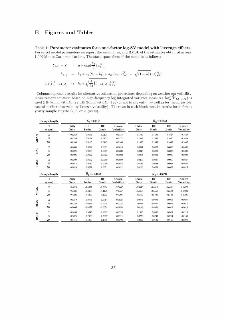
8/3/2019 The In Format In Content of High-Frequency Data for Estimating Equity Return Models
http://slidepdf.com/reader/full/the-in-format-in-content-of-high-frequency-data-for-estimating-equity-return 37/48
B Figures and Tables
Table 1: Parameter estimates for a one-factor log-SV model with leverage effects.For select model parameters we report the mean, bias, and RMSE of the estimates obtained across
1,000 Monte Carlo replications. The state-space form of the model is as follows:
Y t+1 − Y t = µ + exp(ht
2) ε
(1)t+1
ht+1 = ht + κh(θh − ht) + σh (ρh · ε(1)t+1 +
(1− ρ2
h) · ε(2)t+1)
log( IV t,t+1;M ) ≈ ht +
1
M Ωt,t+1;M ε
(IV )t+1
Columns represent results for alternative estimation procedures depending on weather our volatilitymeasurement equation based on high-frequency log integrated variance measures log( IV t,t+1;M ) isused (HF 5-min with M=78; HF 2-min with M=195) or not (daily only), as well as for the infeasiblecase of perfect observability (known volatility). The rows in each block contain results for different
yearly sample lengths (2, 5, or 20 years).
Sample length
T
(years)
Daily
Only
HF
5-min
HF
2-min
Known
Volatility
Daily
Only
HF
5-min
HF
2-min
Known
Volatility
2 0.0249 0.0176 0.0174 0.0173 0.1739 0.1655 0.1647 0.1649
5 0.0188 0.0171 0.0171 0.0171 0.1694 0.1649 0.1650 0.1649
20 0.0168 0.0165 0.0165 0.0165 0.1653 0.1647 0.1647 0.1647
2 0.0086 0.0014 0.0011 0.0010 0.0091 0.0007 0.0000 0.0001
5 0.0025 0.0009 0.0009 0.0008 0.0046 0.0002 0.0002 0.0001
20 0.0006 0.0002 0.0002 0.0002 0.0005 -0.0001 0.0000 0.0000
2 0.0309 0.0092 0.0090 0.0089 0.0260 0.0087 0.0069 0.0047
5 0.0071 0.0050 0.0049 0.0048 0.0183 0.0058 0.0045 0.0030
20 0.0028 0.0021 0.0021 0.0021 0.0100 0.0028 0.0023 0.0015
Sample length
T
(years)
Daily
Only
HF
5-min
HF
2-min
Known
Volatility
Daily
Only
HF
5-min
HF
2-min
Known
Volatility
2 -9.4024 -9.4837 -9.5006 -9.5067 -0.5840 -0.6618 -0.6651 -0.6679
5 -9.4481 -9.4468 -9.4478 -9.4467 -0.6360 -0.6668 -0.6683 -0.6704
20 -9.4308 -9.4299 -9.4297 -9.4295 -0.6599 -0.6709 -0.6703 -0.6706
2 0.0219 -0.0594 -0.0764 -0.0825 0.0875 0.0098 0.0065 0.0037
5 -0.0239 -0.0225 -0.0235 -0.0224 0.0355 0.0047 0.0032 0.0012
20 -0.0065 -0.0057 -0.0054 -0.0053 0.0116 0.0006 0.0012 0.0010
2 0.9659 0.8943 0.8897 0.8720 0.1383 0.0395 0.0321 0.0210
5 0.3026 0.2906 0.2917 0.2911 0.0776 0.0247 0.0214 0.0140
20 0.1416 0.1390 0.1395 0.1398 0.0392 0.0132 0.0110 0.0073
M E A N
B I A S
R M S E
h = 0.0163
M E A N
h = 0.1648
h = - 0.6716
B I A S
R
M S E
h = - 9.4243
32
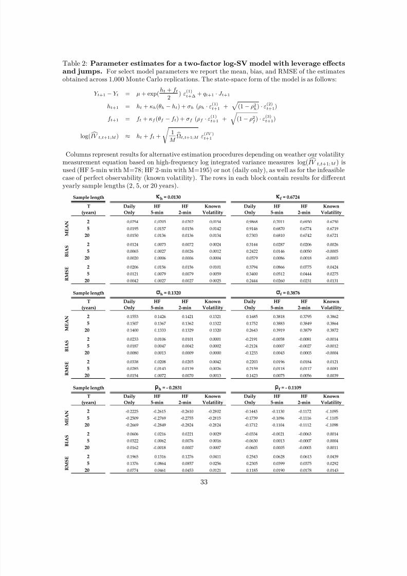
8/3/2019 The In Format In Content of High-Frequency Data for Estimating Equity Return Models
http://slidepdf.com/reader/full/the-in-format-in-content-of-high-frequency-data-for-estimating-equity-return 38/48
Table 2: Parameter estimates for a two-factor log-SV model with leverage effectsand jumps. For select model parameters we report the mean, bias, and RMSE of the estimatesobtained across 1,000 Monte Carlo replications. The state-space form of the model is as follows:
Y t+1
−Y t = µ + exp(
ht + f t
2
) ε(1)t+∆ + qt+1
·J t+1
ht+1 = ht + κh(θh − ht) + σh (ρh · ε(1)t+1 +
(1− ρ2h) · ε
(2)t+1)
f t+1 = f t + κf (θf − f t) + σf (ρf · ε(1)t+1 +
(1− ρ2f ) · ε
(3)t+1)
log( IV t,t+1;M ) ≈ ht + f t +
1
M Ωt,t+1;M ε
(IV )t+1
Columns represent results for alternative estimation procedures depending on weather our volatilitymeasurement equation based on high-frequency log integrated variance measures log( IV t,t+1;M ) isused (HF 5-min with M=78; HF 2-min with M=195) or not (daily only), as well as for the infeasiblecase of perfect observability (known volatility). The rows in each block contain results for differentyearly sample lengths (2, 5, or 20 years).
Sample length
T
(years)
Daily
Only
HF
5-min
HF
2-min
Known
Volatility
Daily
Only
HF
5-min
HF
2-min
Known
Volatility
2 0.0254 0.0203 0.0202 0.0154 0.9868 0.7011 0.6930 0.6750
5 0.0195 0.0157 0.0156 0.0142 0.9146 0.6870 0.6774 0.6719
20 0.0150 0.0136 0.0136 0.0134 0.7303 0.6810 0.6742 0.6721
2 0.0124 0.0073 0.0072 0.0024 0.3144 0.0287 0.0206 0.0026
5 0.0065 0.0027 0.0026 0.0012 0.2422 0.0146 0.0050 -0.0005
20 0.0020 0.0006 0.0006 0.0004 0.0579 0.0086 0.0018 -0.0003
2 0.0206 0.0156 0.0156 0.0101 0.3794 0.0866 0.0775 0.0424
5 0.0121 0.0079 0.0079 0.0059 0.3400 0.0512 0.0444 0.0275
20 0.0042 0.0027 0.0027 0.0025 0.2444 0.0260 0.0231 0.0131
Sample length
T(years)
DailyOnly
HF5-min
HF2-min
KnownVolatility
DailyOnly
HF5-min
HF2-min
KnownVolatility
2 0.1553 0.1426 0.1421 0.1321 0.1685 0.3818 0.3795 0.3862
5 0.1507 0.1367 0.1362 0.1322 0.1752 0.3883 0.3849 0.3864
20 0.1400 0.1333 0.1329 0.1320 0.2643 0.3919 0.3879 0.3872
2 0.0233 0.0106 0.0101 0.0001 -0.2191 -0.0058 -0.0081 -0.0014
5 0.0187 0.0047 0.0042 0.0002 -0.2124 0.0007 -0.0027 -0.0012
20 0.0080 0.0013 0.0009 0.0000 -0.1233 0.0043 0.0003 -0.0004
2 0.0338 0.0208 0.0205 0.0042 0.2203 0.0196 0.0184 0.0121
5 0.0285 0.0143 0.0139 0.0026 0.2159 0.0118 0.0117 0.0081
20 0.0154 0.0072 0.0070 0.0013 0.1423 0.0075 0.0056 0.0039
Sample length
T
(years)
Daily
Only
HF
5-min
HF
2-min
Known
Volatility
Daily
Only
HF
5-min
HF
2-min
Known
Volatility
2 -0.2225 -0.2615 -0.2610 -0.2802 -0.1443 -0.1130 -0.1172 -0.1095
5 -0.2509 -0.2769 -0.2755 -0.2815 -0.1739 -0.1096 -0.1116 -0.1105
20 -0.2669 -0.2849 -0.2824 -0.2824 -0.1712 -0.1104 -0.1112 -0.1098
2 0.0606 0.0216 0.0221 0.0029 -0.0334 -0.0021 -0.0063 0.0014
5 0.0322 0.0062 0.0076 0.0016 -0.0630 0.0013 -0.0007 0.0004
20 0.0162 -0.0018 0.0007 0.0007 -0.0603 0.0005 -0.0003 0.0011
2 0.1965 0.1316 0.1276 0.0411 0.2543 0.0628 0.0613 0.0439
5 0.1376 0.0864 0.0857 0.0256 0.2305 0.0399 0.0375 0.0292
20 0.0774 0.0461 0.0453 0.0121 0.1185 0.0190 0.0178 0.0143 R M S E
h = - 0.2831 f = - 0.1109
M E A N
B I A S
M E A N
B I A S
R M S E
h
= 0.0130
M E A N
f
= 0.6724
f = 0.3876
B I A S
R M S E
h = 0.1320
33
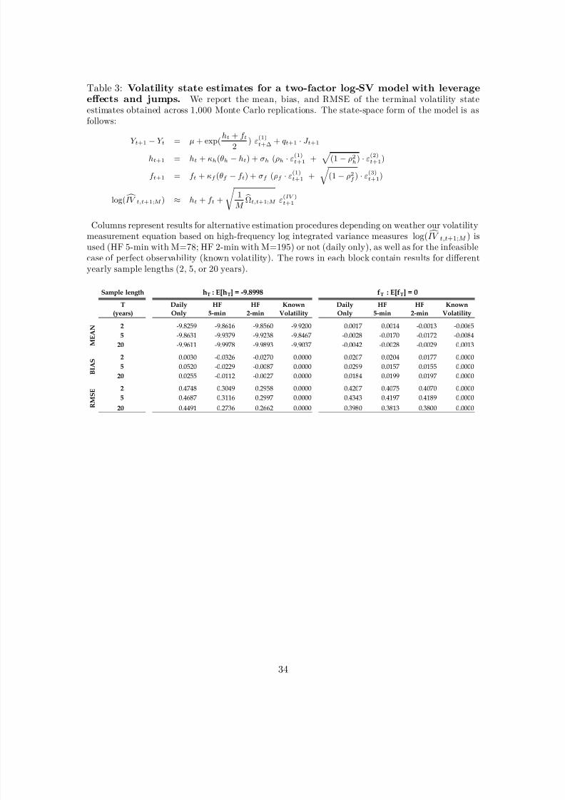
8/3/2019 The In Format In Content of High-Frequency Data for Estimating Equity Return Models
http://slidepdf.com/reader/full/the-in-format-in-content-of-high-frequency-data-for-estimating-equity-return 39/48
Table 3: Volatility state estimates for a two-factor log-SV model with leverageeffects and jumps. We report the mean, bias, and RMSE of the terminal volatility stateestimates obtained across 1,000 Monte Carlo replications. The state-space form of the model is asfollows:
Y t+1 − Y t = µ + exp( ht + f t2 ) ε(1)t+∆ + qt+1 · J t+1
ht+1 = ht + κh(θh − ht) + σh (ρh · ε(1)t+1 +
(1− ρ2h) · ε
(2)t+1)
f t+1 = f t + κf (θf − f t) + σf (ρf · ε(1)t+1 +
(1− ρ2f ) · ε
(3)t+1)
log( IV t,t+1;M ) ≈ ht + f t +
1
M Ωt,t+1;M ε
(IV )t+1
Columns represent results for alternative estimation procedures depending on weather our volatilitymeasurement equation based on high-frequency log integrated variance measures log( IV t,t+1;M ) isused (HF 5-min with M=78; HF 2-min with M=195) or not (daily only), as well as for the infeasiblecase of perfect observability (known volatility). The rows in each block contain results for differentyearly sample lengths (2, 5, or 20 years).
Sample length
T
(years)
Daily
Only
HF
5-min
HF
2-min
Known
Volatility
Daily
Only
HF
5-min
HF
2-min
Known
Volatility
2 -9.8259 -9.8616 -9.8560 -9.9200 0.0017 0.0014 -0.0013 -0.0065
5 -9.8631 -9.9379 -9.9238 -9.8467 -0.0028 -0.0170 -0.0172 -0.0084
20 -9.9611 -9.9978 -9.9893 -9.9037 -0.0042 -0.0028 -0.0029 0.0013
2 0.0030 -0.0326 -0.0270 0.0000 0.0207 0.0204 0.0177 0.0000
5 0.0520 -0.0229 -0.0087 0.0000 0.0299 0.0157 0.0155 0.0000
20 0.0255 -0.0112 -0.0027 0.0000 0.0184 0.0199 0.0197 0.0000
2 0.4748 0.3049 0.2958 0.0000 0.4207 0.4075 0.4070 0.0000
5 0.4687 0.3116 0.2997 0.0000 0.4343 0.4197 0.4189 0.0000
20 0.4491 0.2736 0.2662 0.0000 0.3980 0.3813 0.3800 0.0000
hT : E[hT] = -9.8998 fT : E[fT] = 0
M E A N
B I A S
R M S E
34
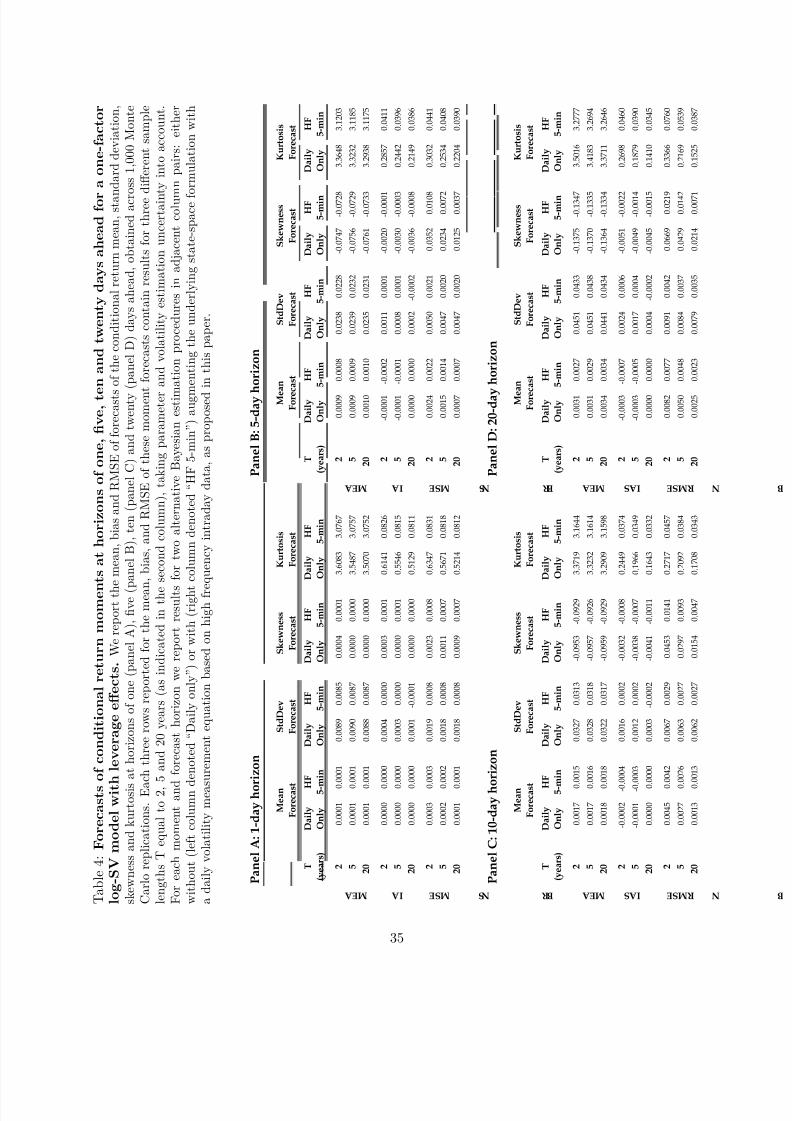
8/3/2019 The In Format In Content of High-Frequency Data for Estimating Equity Return Models
http://slidepdf.com/reader/full/the-in-format-in-content-of-high-frequency-data-for-estimating-equity-return 40/48
T a b l e 4 : F o r e c a s t s o
f c o n d i t i o n a l r e t u r n m o m e n t s a t h o r i z o n s o f o n e , fi v e , t e n a n d t w e n t y d a y s a h e a d f o r
a o n e - f a c t o r
l o g - S V m o d e l w i t h
l e v e r a g e e ff e c t s . W e r e p o r t t h e
m e a n , b i a s a n d R M S E o f f o r e c a s t s o f t h e c o n d i t i o n a l r e t u r n m e a n , s t a n
d a r d d e v i a t i o n ,
s k e w n e s s a n d k u r t o s i s a
t h o r i z o n s o f o n e ( p a n e l A ) , fi v e ( p a n e l B ) , t e n ( p a n e l C ) a n d t w e n t y ( p a n e l D ) d a y s a h e a d , o b t a i n e d a c r o s s 1 , 0 0 0 M o n t e
C a r l o r e p l i c a t i o n s . E a c h t h r e e r o w s r e p o r t e d f o r t h e m e a n , b i a s , a n d R M S E o f t h e s e m o m e n t
f o r e c a s t s c o n t a i n r e s u l t s f o r t h r e e d i ff e r e n t s a m p l e
l e n g t h s T e q u a l t o 2 , 5
a n d 2 0 y e a r s ( a s i n d i c a t e d i n t h e s e c o n d c o l u m n ) , t a k i n g p a r a m e t e r a n d v o l a t i l i t y e s t i m a t i o n u n c e r t a i n t y i n t o a c c o u n t .
F o r e a c h m o m e n t a n d
f o r e c a s t h o r i z o n w e r e p o r t r e s u l t s
f o r t w o a l t e r n a t i v e B a y e s i a n e s t i m a t i o n p r o c e d u r e s i n a d j a c e n t c o l u m
n p a i r s : e i t h e r
w i t h o u t ( l e f t c o l u m n d e
n o t e d “ D a i l y o n l y ” ) o r w i t h ( r i g h t c o l u m n d e n o t e d “ H F 5 - m i n ” ) a u g m
e n t i n g t h e u n d e r l y i n g s t a t e - s p a c e f o
r m u l a t i o n w i t h
a d a i l y v o l a t i l i t y m e a s u
r e m e n t e q u a t i o n b a s e d o n h i g h f r e q u e n c y i n t r a d a y d a t a , a s p r o p o s e d i n t h i s p a p e r .
T ( y e a r s )
D a i l y
O n l y
H F 5 - m i n
D a i l y
O n l y
H F
5 - m i n
D a i l y
O n l y
H F
5 - m i n
D a i l y
O n l y
H F
5 - m i n
T ( y e a r s )
D a i l y
O n l y
H F
5 - m i n
D a i l y
O n l y
H F
5 - m i n
D a i l y
O n l y
H F
5 - m i n
D a i l y
O n l y
H F
5 - m i n
2
0 . 0
0 0 1
0 . 0
0 0 1
0 . 0
0 8 9
0 . 0
0 8 5
0 . 0
0 0 4
0 . 0
0 0 1
3 . 6
0 8 3
3 . 0
7 6 7
2
0 . 0
0 0 9
0 . 0
0 0 8
0 . 0
2 3 8
0 . 0
2 2 8
- 0 . 0
7 4 7
- 0 . 0
7 2 8
3 . 3
6 4 8
3 . 1
2 0 3
5
0 . 0
0 0 1
0 . 0
0 0 1
0 . 0
0 9 0
0 . 0
0 8 7
0 . 0
0 0 0
0 . 0
0 0 0
3 . 5
4 8 7
3 . 0
7 5 7
5
0 . 0
0 0 9
0 . 0
0 0 9
0 . 0
2 3 9
0 . 0
2 3 2
- 0 . 0
7 5 6
- 0 . 0
7 2 9
3 . 3
2 3 2
3 . 1
1 8 5
2 0
0 . 0
0 0 1
0 . 0
0 0 1
0 . 0
0 8 8
0 . 0
0 8 7
0 . 0
0 0 0
0 . 0
0 0 0
3 . 5
0 7 0
3 . 0
7 5 2
2 0
0 . 0
0 1 0
0 . 0
0 1 0
0 . 0
2 3 5
0 . 0
2 3 1
- 0 . 0
7 6 1
- 0 . 0
7 3 3
3 . 2
9 3 8
3 . 1
1 7 5
2
0 . 0
0 0 0
0 . 0
0 0 0
0 . 0
0 0 4
0 . 0
0 0 0
0 . 0
0 0 3
0 . 0
0 0 1
0 . 6
1 4 1
0 . 0
8 2 6
2
- 0 . 0
0 0 1
- 0 . 0
0 0 2
0 . 0
0 1 1
0 . 0
0 0 1
- 0 . 0
0 2 0
- 0 . 0
0 0 1
0 . 2
8 5 7
0 . 0
4 1 1
5
0 . 0
0 0 0
0 . 0
0 0 0
0 . 0
0 0 3
0 . 0
0 0 0
0 . 0
0 0 0
0 . 0
0 0 1
0 . 5
5 4 6
0 . 0
8 1 5
5
- 0 . 0
0 0 1
- 0 . 0
0 0 1
0 . 0
0 0 8
0 . 0
0 0 1
- 0 . 0
0 3 0
- 0 . 0
0 0 3
0 . 2
4 4 2
0 . 0
3 9 6
2 0
0 . 0
0 0 0
0 . 0
0 0 0
0 . 0
0 0 1
- 0 . 0
0 0 1
0 . 0
0 0 0
0 . 0
0 0 0
0 . 5
1 2 9
0 . 0
8 1 1
2 0
0 . 0
0 0 0
0 . 0
0 0 0
0 . 0
0 0 2
- 0 . 0
0 0 2
- 0 . 0
0 3 6
- 0 . 0
0 0 8
0 . 2
1 4 9
0 . 0
3 8 6
2
0 . 0
0 0 3
0 . 0
0 0 3
0 . 0
0 1 9
0 . 0
0 0 8
0 . 0
0 2 3
0 . 0
0 0 8
0 . 6
3 4 7
0 . 0
8 3 1
2
0 . 0
0 2 4
0 . 0
0 2 2
0 . 0
0 5 0
0 . 0
0 2 1
0 . 0
3 5 2
0 . 0
1 0 8
0 . 3
0 3 2
0 . 0
4 4 1
5
0 . 0
0 0 2
0 . 0
0 0 2
0 . 0
0 1 8
0 . 0
0 0 8
0 . 0
0 1 1
0 . 0
0 0 7
0 . 5
6 7 1
0 . 0
8 1 8
5
0 . 0
0 1 5
0 . 0
0 1 4
0 . 0
0 4 7
0 . 0
0 2 0
0 . 0
2 3 4
0 . 0
0 7 2
0 . 2
5 3 4
0 . 0
4 0 8
2 0
0 . 0
0 0 1
0 . 0
0 0 1
0 . 0
0 1 8
0 . 0
0 0 8
0 . 0
0 0 9
0 . 0
0 0 7
0 . 5
2 1 4
0 . 0
8 1 2
2 0
0 . 0
0 0 7
0 . 0
0 0 7
0 . 0
0 4 7
0 . 0
0 2 0
0 . 0
1 2 5
0 . 0
0 3 7
0 . 2
2 0 4
0 . 0
3 9 0
T ( y e a r s )
D a i l y
O n l y
H F 5 - m i n
D a i l y
O n l y
H F
5 - m i n
D a i l y
O n l y
H F
5 - m i n
D a i l y
O n l y
H F
5 - m i n
T ( y e a r s )
D a i l y
O n l y
H F
5 - m i n
D a i l y
O n l y
H F
5 - m i n
D a i l y
O n l y
H F
5 - m i n
D a i l y
O n l y
H F
5 - m i n
2
0 . 0
0 1 7
0 . 0
0 1 5
0 . 0
3 2 7
0 . 0
3 1 3
- 0 . 0
9 5 3
- 0 . 0
9 2 9
3 . 3
7 1 9
3 . 1
6 4 4
2
0 . 0
0 3 1
0 . 0
0 2 7
0 . 0
4 5 1
0 . 0
4 3 3
- 0 . 1
3 7 5
- 0 . 1
3 4 7
3 . 5
0 1 6
3 . 2
7 7 7
5
0 . 0
0 1 7
0 . 0
0 1 6
0 . 0
3 2 8
0 . 0
3 1 8
- 0 . 0
9 5 7
- 0 . 0
9 2 6
3 . 3
2 3 2
3 . 1
6 1 4
5
0 . 0
0 3 1
0 . 0
0 2 9
0 . 0
4 5 1
0 . 0
4 3 8
- 0 . 1
3 7 0
- 0 . 1
3 3 5
3 . 4
1 8 3
3 . 2
6 9 4
2 0
0 . 0
0 1 8
0 . 0
0 1 8
0 . 0
3 2 2
0 . 0
3 1 7
- 0 . 0
9 5 9
- 0 . 0
9 2 9
3 . 2
9 0 9
3 . 1
5 9 8
2 0
0 . 0
0 3 4
0 . 0
0 3 4
0 . 0
4 4 1
0 . 0
4 3 4
- 0 . 1
3 6 4
- 0 . 1
3 3 4
3 . 3
7 1 1
3 . 2
6 4 6
2
- 0 . 0
0 0 2
- 0 . 0
0 0 4
0 . 0
0 1 6
0 . 0
0 0 2
- 0 . 0
0 3 2
- 0 . 0
0 0 8
0 . 2
4 4 9
0 . 0
3 7 4
2
- 0 . 0
0 0 3
- 0 . 0
0 0 7
0 . 0
0 2 4
0 . 0
0 0 6
- 0 . 0
0 5 1
- 0 . 0
0 2 2
0 . 2
6 9 8
0 . 0
4 6 0
5
- 0 . 0
0 0 1
- 0 . 0
0 0 3
0 . 0
0 1 2
0 . 0
0 0 2
- 0 . 0
0 3 8
- 0 . 0
0 0 7
0 . 1
9 6 6
0 . 0
3 4 9
5
- 0 . 0
0 0 3
- 0 . 0
0 0 5
0 . 0
0 1 7
0 . 0
0 0 4
- 0 . 0
0 4 9
- 0 . 0
0 1 4
0 . 1
8 7 9
0 . 0
3 9 0
2 0
0 . 0
0 0 0
0 . 0
0 0 0
0 . 0
0 0 3
- 0 . 0
0 0 2
- 0 . 0
0 4 1
- 0 . 0
0 1 1
0 . 1
6 4 3
0 . 0
3 3 2
2 0
0 . 0
0 0 0
0 . 0
0 0 0
0 . 0
0 0 4
- 0 . 0
0 0 2
- 0 . 0
0 4 5
- 0 . 0
0 1 5
0 . 1
4 1 0
0 . 0
3 4 5
2
0 . 0
0 4 5
0 . 0
0 4 2
0 . 0
0 6 7
0 . 0
0 2 9
0 . 0
4 5 3
0 . 0
1 4 1
0 . 2
7 1 7
0 . 0
4 5 7
2
0 . 0
0 8 2
0 . 0
0 7 7
0 . 0
0 9 1
0 . 0
0 4 2
0 . 0
6 6 9
0 . 0
2 1 9
0 . 3
3 6 6
0 . 0
7 6 0
5
0 . 0
0 2 7
0 . 0
0 2 6
0 . 0
0 6 3
0 . 0
0 2 7
0 . 0
2 9 7
0 . 0
0 9 3
0 . 2
0 9 2
0 . 0
3 8 4
5
0 . 0
0 5 0
0 . 0
0 4 8
0 . 0
0 8 4
0 . 0
0 3 7
0 . 0
4 2 9
0 . 0
1 4 2
0 . 2
1 6 9
0 . 0
5 3 9
2 0
0 . 0
0 1 3
0 . 0
0 1 3
0 . 0
0 6 2
0 . 0
0 2 7
0 . 0
1 5 4
0 . 0
0 4 7
0 . 1
7 0 8
0 . 0
3 4 3
2 0
0 . 0
0 2 5
0 . 0
0 2 3
0 . 0
0 7 9
0 . 0
0 3 5
0 . 0
2 1 4
0 . 0
0 7 1
0 . 1
5 2 5
0 . 0
3 8 7
P a n e l A : 1 - d a y h o r i
z o n
P a n e l B : 5 - d a y h
o r i z o n
M E A N I A S
R M S E
R M S E
M e a n
F o r e c a s t
S t d D e v
F o r e c a s t
S k e w n e s s
F o r e c a s t
K u r t o s i s
F o r e c a s t
M e a
n
F o r e c a s t
S t d D e v
F o r e c a s t
S k e w n e s s
F o r e c a s t
K u r t o s i s
F o r e c a s t
P a n e l D : 2 0 - d a y
h o r i z o n
M e a
n
F o r e c a s t
S t d D e v
F o r e c a s t
S k e w n e s s
F o r e c a s t
K u r t o s i s
F o r e c a s t
M e a n
F o r e c a s t
S t d D e v
F o r e c a s t
K u r t o s i s
F o r e c a s t
S k e w n e s s
F o r e c a s t
M E A N B I A S R M S E
M E A N I A S M E A N B I A S R M S E
P a n e l C : 1 0 - d a y h o r i z o n
35
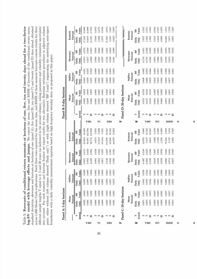
8/3/2019 The In Format In Content of High-Frequency Data for Estimating Equity Return Models
http://slidepdf.com/reader/full/the-in-format-in-content-of-high-frequency-data-for-estimating-equity-return 41/48
T a b l e 5 : F o r e c a s t s o
f c o n d i t i o n a l r e t u r n m o m e n t s a t h o r i z o n s o f o n e , fi v e , t e n a n d t w e n t y d a y s a h e a d f o r
a t w o - f a c t o r
l o g - S V
m o d e l w i t h
l e v e r a g e e ff e c t s a n d j u m p s
. W e r e p o r t t h e m e a n , b i a s a n d R
M S E o f f o r e c a s t s o f t h e c o n d i t i o n a l r e t u r n m e a n ,
s t a n d a r d d e v i a t i o n , s k e w n e s s a n d k u r t o s i s a t h o r i z o n s o f o n e ( p a n e l A ) , fi v e ( p a n e l B ) , t e n ( p a n e l C ) a n d t w e n t y ( p a n e l D ) d a y s a h e a d , o b t a i n e d
a c r o s s 1 , 0 0 0 M o n t e C a r l o r e p l i c a t i o n s . E a c h t h r e e r o w s r e p o r t e d f o r t h e m e a n , b i a s , a n d R M S E
o f t h e s e m o m e n t f o r e c a s t s c o n t a i n r e s u l t s f o r t h r e e
d i ff e r e n t s a m p l e l e n g t h s T e q u a l t o 2 , 5 a n d 2 0 y e a r s ( a s i n
d i c a t e d i n t h e s e c o n d c o l u m n ) , t a k i n g p a r a m e t e r a n d v o l a t i l i t y e s t i m a t
i o n u n c e r t a i n t y
i n t o a c c o u n t . F o r e a c h
m o m e n t a n d f o r e c a s t h o r i z o n w e r e p o r t r e s u l t s f o r t w o a l t e r n a t i v e B
a y e s i a n e s t i m a t i o n p r o c e d u r e s i n a
d j a c e n t c o l u m n
p a i r s : e i t h e r w i t h o u t ( l e f t c o l u m n d e n o t e d “ D a i l y o n l y ” )
o r w i t h ( r i g h t c o l u m n d e n o t e d “ H
F 5 - m i n ” ) a u g m e n t i n g t h e u n d e r l y
i n g s t a t e - s p a c e
f o r m u l a t i o n w i t h a d a i l y v o l a t i l i t y m e a s u r e m e n t e q u a t i o n b a s e d o n h i g h f r e q u e n c y i n t r a d a y d
a t a , a s p r o p o s e d i n t h i s p a p e r .
T ( y e a r s )
D a i l y
O n l y
H F 5 - m i n
D a i l y
O n l y
H F
5 - m i n
D a i l y
O n l y
H F
5 - m i n
D a i l y
O n l y
H F
5 - m i n
T ( y e a r s )
D a i l y
O n l y
H F
5 - m i n
D a i l y
O n l y
H F
5 - m i n
D a i l y
O n l y
H F
5 - m i n
D a i l y
O n l y
H F
5 - m i n
2
0 . 0
0 0 5
0 . 0
0 0 5
0 . 0
0 9 9
0 . 0
0 9 8
- 0 . 5
8 3 1
- 0 . 6
1 7 3
9 2 . 9
0 5 9
9 6 . 2
4 5 0
2
0 . 0
0 3 8
0 . 0
0 3 8
0 . 0
2 6 4
0 . 0
2 6 1
- 0 . 2
4 7 3
- 0 . 2
7 2 2
1 7 . 1
5 6 2
1 5 . 8
0 9 2
5
0 . 0
0 0 6
0 . 0
0 0 5
0 . 0
0 9 7
0 . 0
0 9 5
- 0 . 5
9 2 3
- 0 . 6
5 2 0
9 0 . 2
9 7 1
1 0 2 . 7
3 8 4
5
0 . 0
0 3 9
0 . 0
0 3 8
0 . 0
2 5 8
0 . 0
2 5 3
- 0 . 2
6 1 7
- 0 . 2
8 4 0
1 5 . 0
4 7 5
1 6 . 6
9 6 8
2 0
0 . 0
0 0 6
0 . 0
0 0 6
0 . 0
0 9 5
0 . 0
0 9 4
- 0 . 6
3 8 2
- 0 . 6
9 5 6
9 8 . 1
7 7 6
1 1 0 . 3
5 6 8
2 0
0 . 0
0 4 0
0 . 0
0 3 9
0 . 0
2 5 1
0 . 0
2 4 9
- 0 . 2
8 0 0
- 0 . 2
9 7 3
1 6 . 1
2 9 3
1 7 . 7
0 1 2
2
0 . 0
0 0 0
0 . 0
0 0 0
0 . 0
0 0 0
- 0 . 0
0 0 1
0 . 0
5 0 1
0 . 0
1 5 8
- 6 . 8
1 7 3
- 3 . 4
7 8 1
2
- 0 . 0
0 0 1
- 0 . 0
0 0 1
0 . 0
0 0 2
0 . 0
0 0 0
0 . 0
2 8 6
0 . 0
0 3 6
0 . 9
1 6 0
- 0 . 4
3 1 0
5
0 . 0
0 0 0
0 . 0
0 0 0
0 . 0
0 0 2
0 . 0
0 0 0
0 . 0
8 2 4
0 . 0
2 2 6
- 1 7 . 8
1 1 0
- 5 . 3
6 9 8
5
- 0 . 0
0 0 1
- 0 . 0
0 0 1
0 . 0
0 0 5
- 0 . 0
0 0 1
0 . 0
2 8 7
0 . 0
0 6 6
- 2 . 3
0 4 8
- 0 . 6
7 7 6
2 0
0 . 0
0 0 0
0 . 0
0 0 0
0 . 0
0 0 1
0 . 0
0 0 0
0 . 0
8 7 1
0 . 0
2 9 7
- 1 9 . 4
3 1 4
- 7 . 2
5 2 1
2 0
0 . 0
0 0 0
- 0 . 0
0 0 1
0 . 0
0 0 2
0 . 0
0 0 0
0 . 0
2 5 7
0 . 0
0 8 4
- 2 . 5
0 7 5
- 0 . 9
3 5 6
2
0 . 0
0 0 3
0 . 0
0 0 3
0 . 0
0 2 0
0 . 0
0 1 2
0 . 3
1 2 8
0 . 2
0 0 7
1 1 4 . 2
7 9 5
3 6 . 3
3 6 7
2
0 . 0
0 2 2
0 . 0
0 2 0
0 . 0
0 5 2
0 . 0
0 3 1
0 . 1
7 6 6
0 . 0
6 2 1
5 1 . 3
5 4 7
4 . 9
1 7 3
5
0 . 0
0 0 2
0 . 0
0 0 2
0 . 0
0 1 7
0 . 0
0 1 2
0 . 3
0 4 2
0 . 1
9 8 1
6 0 . 8
2 9 1
3 9 . 1
5 2 5
5
0 . 0
0 1 3
0 . 0
0 1 2
0 . 0
0 4 4
0 . 0
0 3 0
0 . 1
0 0 9
0 . 0
6 4 2
8 . 1
9 6 3
5 . 2
4 6 7
2 0
0 . 0
0 0 1
0 . 0
0 0 1
0 . 0
0 1 5
0 . 0
0 1 0
0 . 3
0 8 5
0 . 1
9 2 4
6 4 . 5
2 7 0
3 7 . 8
0 3 2
2 0
0 . 0
0 0 6
0 . 0
0 0 6
0 . 0
0 3 9
0 . 0
0 2 5
0 . 1
0 0 1
0 . 0
5 8 9
8 . 6
5 2 9
5 . 0
5 0 7
T ( y e a r s )
D a i l y
O n l y
H F 5 - m i n
D a i l y
O n l y
H F
5 - m i n
D a i l y
O n l y
H F
5 - m i n
D a i l y
O n l y
H F
5 - m i n
T ( y e a r s )
D a i l y
O n l y
H F
5 - m i n
D a i l y
O n l y
H F
5 - m i n
D a i l y
O n l y
H F
5 - m i n
D a i l y
O n l y
H F
5 - m i n
2
0 . 0
0 7 1
0 . 0
0 7 1
0 . 0
3 6 2
0 . 0
3 5 8
- 0 . 1
9 8 7
- 0 . 2
1 4 9
1 0 . 8
7 9 2
9 . 6
9 8 5
2
0 . 0
1 3 2
0 . 0
1 3 0
0 . 0
4 9 8
0 . 0
4 9 2
- 0 . 1
7 1 8
- 0 . 1
8 1 1
7 . 0
7 2 7
6 . 5
2 3 1
5
0 . 0
0 7 2
0 . 0
0 7 1
0 . 0
3 5 3
0 . 0
3 4 6
- 0 . 2
0 7 0
- 0 . 2
2 2 0
9 . 3
1 3 7
1 0 . 1
3 6 3
5
0 . 0
1 3 3
0 . 0
1 3 0
0 . 0
4 8 4
0 . 0
4 7 4
- 0 . 1
7 6 5
- 0 . 1
8 4 8
6 . 3
4 6 5
6 . 7
1 1 1
2 0
0 . 0
0 7 3
0 . 0
0 7 2
0 . 0
3 4 4
0 . 0
3 4 1
- 0 . 2
1 9 8
- 0 . 2
3 0 6
9 . 8
6 3 1
1 0 . 6
3 6 7
2 0
0 . 0
1 3 6
0 . 0
1 3 3
0 . 0
4 7 0
0 . 0
4 6 6
- 0 . 1
8 4 2
- 0 . 1
8 9 2
6 . 5
9 0 2
6 . 9
3 1 6
2
- 0 . 0
0 0 2
- 0 . 0
0 0 3
0 . 0
0 0 5
0 . 0
0 0 1
0 . 0
1 6 9
0 . 0
0 0 7
1 . 0
0 4 8
- 0 . 1
7 5 9
2
- 0 . 0
0 0 4
- 0 . 0
0 0 5
0 . 0
0 1 0
0 . 0
0 0 4
0 . 0
0 7 3
- 0 . 0
0 2 1
0 . 5
3 3 1
- 0 . 0
1 6 6
5
- 0 . 0
0 0 1
- 0 . 0
0 0 3
0 . 0
0 0 7
0 . 0
0 0 0
0 . 0
1 8 4
0 . 0
0 3 6
- 1 . 1
2 0 4
- 0 . 3
0 9 0
5
- 0 . 0
0 0 2
- 0 . 0
0 0 5
0 . 0
0 1 0
0 . 0
0 0 1
0 . 0
0 8 4
0 . 0
0 0 3
- 0 . 4
6 1 4
- 0 . 1
0 2 1
2 0
0 . 0
0 0 0
- 0 . 0
0 0 1
0 . 0
0 0 3
0 . 0
0 0 0
0 . 0
1 5 8
0 . 0
0 5 0
- 1 . 2
1 8 6
- 0 . 4
4 5 0
2 0
0 . 0
0 0 0
- 0 . 0
0 0 2
0 . 0
0 0 4
0 . 0
0 0 0
0 . 0
0 7 0
0 . 0
0 1 9
- 0 . 5
2 8 9
- 0 . 1
8 7 5
2
0 . 0
0 4 0
0 . 0
0 3 7
0 . 0
0 6 9
0 . 0
0 4 2
0 . 0
9 8 6
0 . 0
4 4 3
3 5 . 4
5 4 1
2 . 5
3 0 9
2
0 . 0
0 7 4
0 . 0
0 6 7
0 . 0
0 9 2
0 . 0
0 5 8
0 . 0
7 2 9
0 . 0
3 5 3
1 4 . 6
6 8 1
1 . 2
7 1 5
5
0 . 0
0 2 4
0 . 0
0 2 2
0 . 0
0 5 9
0 . 0
0 4 0
0 . 0
7 1 0
0 . 0
4 3 6
4 . 1
7 0 2
2 . 6
7 4 4
5
0 . 0
0 4 4
0 . 0
0 4 1
0 . 0
0 7 7
0 . 0
0 5 2
0 . 0
5 1 5
0 . 0
2 9 8
2 . 0
3 2 2
1 . 3
2 0 5
2 0
0 . 0
0 1 2
0 . 0
0 1 1
0 . 0
0 5 1
0 . 0
0 3 2
0 . 0
6 7 9
0 . 0
3 9 5
4 . 3
6 8 5
2 . 5
4 9 5
2 0
0 . 0
0 2 2
0 . 0
0 2 0
0 . 0
0 6 5
0 . 0
0 4 1
0 . 0
4 3 2
0 . 0
2 5 2
2 . 0
9 1 5
1 . 2
2 6 7
M E A N B I A S R M S E
M E A N I A S M E A N B I A S R M S E
P a n e l C : 1 0 - d a y h o r i z o n
S t d D e v
F o r e c a s t
S k e w n e s s
F o r e c a s t
K u r t o s i s
F o r e c a s t
M e a n
F o r e c a s t
S t d D e v
F o r e c a s t
K u r t o s i s
F o r e c a s t
S k e w n e s s
F o r e c a s t
P a n e l A : 1 - d a y h o r i
z o n
P a n e l B : 5 - d a y h
o r i z o n
M E A N I A S
R M S E
R M S E
M e a n
F o r e c a s t
S t d D e v
F o r e c a s t
S k e w n e s s
F o r e c a s t
K u r t o s i s
F o r e c a s t
M e a
n
F o r e c a s t
S t d D e v
F o r e c a s t
S k e w n e s s
F o r e c a s t
K u r t o s i s
F o r e c a s t
P a n e l D : 2 0 - d a y
h o r i z o n
M e a
n
F o r e c a s t
36
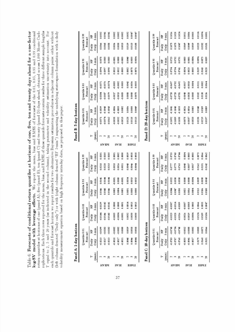
8/3/2019 The In Format In Content of High-Frequency Data for Estimating Equity Return Models
http://slidepdf.com/reader/full/the-in-format-in-content-of-high-frequency-data-for-estimating-equity-return 42/48
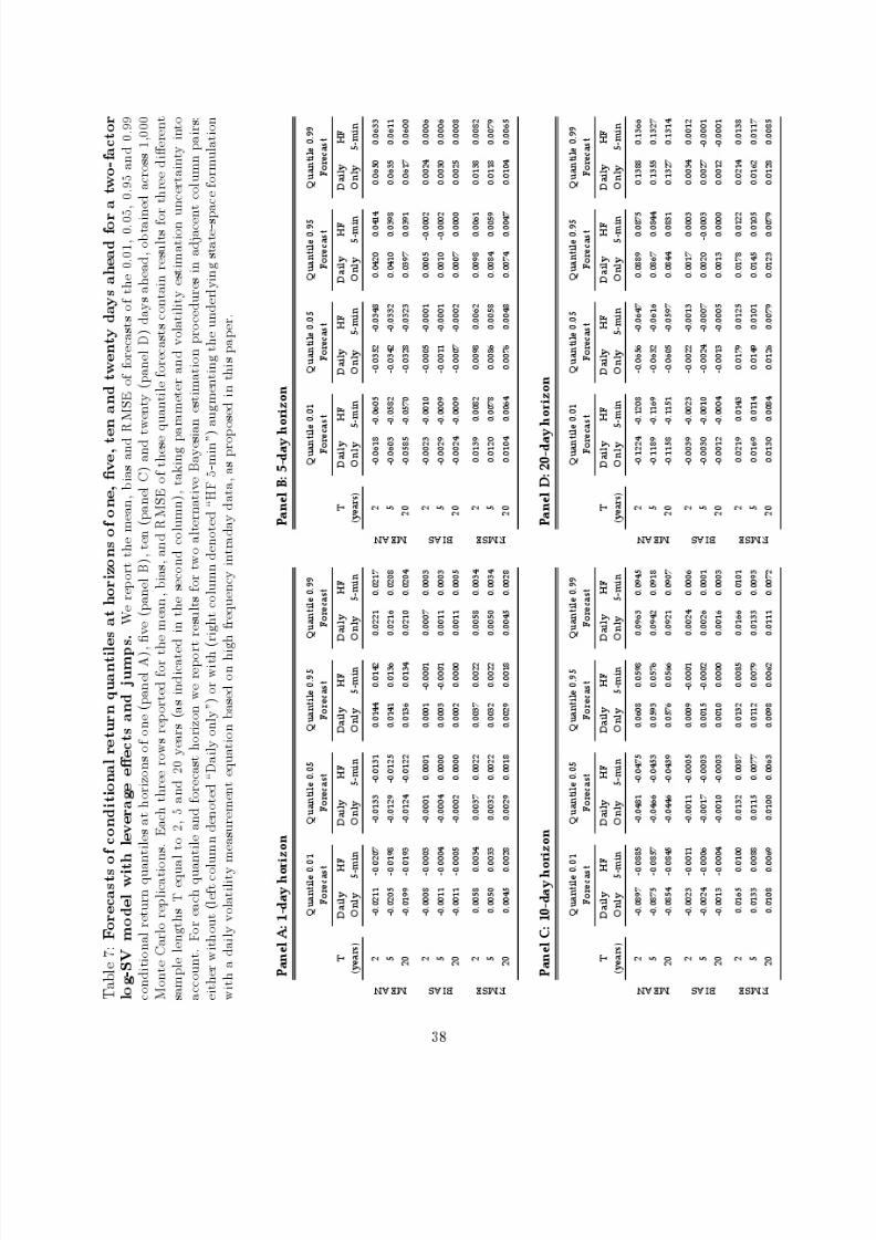
8/3/2019 The In Format In Content of High-Frequency Data for Estimating Equity Return Models
http://slidepdf.com/reader/full/the-in-format-in-content-of-high-frequency-data-for-estimating-equity-return 43/48
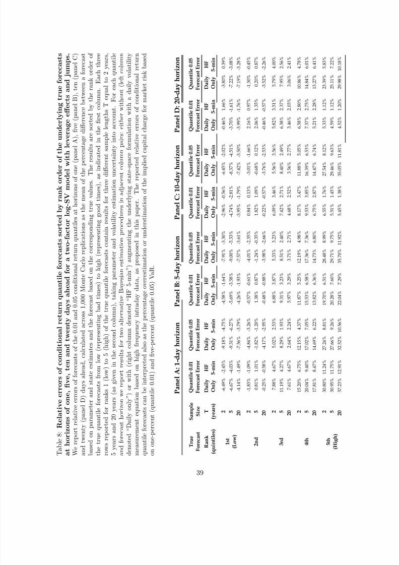
8/3/2019 The In Format In Content of High-Frequency Data for Estimating Equity Return Models
http://slidepdf.com/reader/full/the-in-format-in-content-of-high-frequency-data-for-estimating-equity-return 44/48
T a b l e 8 : R e l a t i v e e r
r o r s o f c o n d i t i o n a l r e t u r n q u
a n t i l e f o r e c a s t s s o r t e d b y r a n k o r d e r o f t h e u n d e r l y i n g t r u e f o r e c a s t s
a t h o r i z o n s o f o n e ,
fi v e , t e n a n d t w e n t y d a y s a h e a d f o r a t w o - f a c t o r l o g - S V
m o d e l w i t h l e v e r a g e e ff e c t s
a n d j u m p s .
W e r e p o r t r e l a t i v e e r r o r s o f f o r e c a s t s o f t h e 0 . 0 1 a n d 0 . 0 5 c o n d i t i o n a l r e t u r n q u a n t i l e s a t h o r i z o n s o f o n e ( p a n e l A ) , fi v e ( p a n e l B ) , t e n ( p a n e l C )
a n d t w e n t y ( p a n e l D ) d
a y s a h e a d , c a l c u l a t e d a c r o s s 1 , 0 0 0
M o n t e C a r l o r e p l i c a t i o n s a s t h e m e a n o f t h e p e r c e n t a g e d i ff e r e n c e b e t
w e e n a f o r e c a s t
b a s e d o n p a r a m e t e r a n
d s t a t e e s t i m a t e s a n d t h e f o r e c a s t
b a s e d o n t h e c o r r e s p o n d i n g t r u e v a l u e s . T h e r e s u l t s a r e s o r t e d b y t h
e r a n k o r d e r o f
t h e t r u e q u a n t i l e f o r e c a s t s f r o m l o w ( r e p r e s e n t i n g b a d t i m
e s ) t o h i g h ( r e p r e s e n t i n g g o o d t i m
e s ) , a s i n d i c a t e d i n t h e fi r s t c o l u m
n . E a c h t h r e e
r o w s r e p o r t e d f o r r a n k s 1 ( l o w ) t o 5 ( h i g h ) o f t h e t r u e q u
a n t i l e f o r e c a s t s c o n t a i n r e s u l t s f o r
t h r e e d i ff e r e n t s a m p l e l e n g t h s T e q u a l t o 2 y e a r s ,
5 y e a r s a n d 2 0 y e a r s ( a s g i v e n i n t h e s e c o n d c o l u m n ) , t a k i n g p a r a m e t e r a n d v o l a t i l i t y e s t i m
a t i o n u n c e r t a i n t y i n t o a c c o u n t . F o
r e a c h q u a n t i l e
a n d f o r e c a s t h o r i z o n w e r e p o r t r e s u l t s f o r t w o a l t e r n a t i v e B a y e s i a n e s t i m a t i o n p r o c e d u r e s i n a d j a c e n t c o l u m n p a i r s : e i t h e r w i t h o
u t ( l e f t c o l u m n
d e n o t e d “ D a i l y o n l y ” )
o r w i t h ( r i g h t c o l u m n d e n o t e d “ H F 5 - m i n ” ) a u g m e n t i n g t h e u n d e r l y i n g s t a t e - s p a c e f o r m u l a t i o n w i t h a
d a i l y v o l a t i l i t y
m e a s u r e m e n t e q u a t i o n
b a s e d o n h i g h f r e q u e n c y i n t r a d a y
d a t a , a s p r o p o s e d i n t h i s p a p e r .
T h e r e p o r t e d r e l a t i v e e r r o r s o f c o n
d i t i o n a l r e t u r n
q u a n t i l e f o r e c a s t s c a n b
e i n t e r p r e t e d a l s o a s t h e p e r c e n t a g e o v e r e s t i m a t i o n o r u n d e r s t i m a t i o n
o f t h e i m p l i e d c a p i t a l c h a r g e f o r m a r k e t r i s k b a s e d
o n o n e - p e r c e n t ( q u a n t i l e 0 . 0 1 ) a n d fi v e - p e r c e n t ( q u a n t i l e 0
. 0 5 ) V a R .
P
a n e l A : 1 - d a y h o r i z o n
P a n e
l B : 5 - d a y h o r i z o n
P a n e l C : 1 0 - d a y h o r i z o n
P a n e l D : 2 0 - d a y h o r i z o n
T r u e
F o r e c a s t
S a m p l e
S i z e
R a n k
( q u i n t i l e s )
T
( y e a r s )
D a i l y
O n l y
H F
5 - m i n
D a i l y
O n l y
H F
5 - m i n
D a i l y
O n l y
H F
5 - m i n
D a i l y
O n l y
H F
5 - m i n
D a i l y
O n l y
H
F
5 - m i n
D a i l y
O n l y
H F
5 - m i n
D a i l y
O n l y
H F
5 - m i n
D a i l y
O n l y
H F
5 - m i n
2
- 6 . 4
9 %
- 2 . 4
5 %
- 9 . 1
8 %
- 4 . 7
5 %
- 4 . 5 8 %
- 1 . 6
4 %
- 7 . 9
1 %
- 3 . 3
0 %
- 2 . 9
6 %
- 0
. 5 6 %
- 6 . 4
5 %
- 2 . 0
2 %
- 0 . 4
6 %
1 . 6
6 %
- 3 . 8
0 %
0 . 3
9 %
5
- 6 . 6
7 %
- 4 . 0
3 %
- 9 . 3
1 %
- 6 . 2
7 %
- 5 . 6 9 %
- 3 . 5
8 %
- 9 . 0
0 %
- 5 . 3
3 %
- 4 . 7
4 %
- 2
. 8 1 %
- 8 . 3
7 %
- 4 . 5
1 %
- 3 . 7
0 %
- 1 . 6
1 %
- 7 . 2
2 %
- 3 . 0
8 %
2 0
- 4 . 1
4 %
- 1 . 4
9 %
- 7 . 5
6 %
- 3 . 7
9 %
- 4 . 2 6 %
- 1 . 9
3 %
- 7 . 5
7 %
- 3 . 6
1 %
- 3 . 9
5 %
- 1
. 7 9 %
- 7 . 4
2 %
- 3 . 5
0 %
- 3 . 9
9 %
- 1 . 7
6 %
- 7 . 1
9 %
- 3 . 2
8 %
2
- 1 . 8
3 %
- 1 . 0
9 %
- 4 . 8
4 %
- 3 . 2
6 %
- 0 . 5 7 %
- 0 . 6
1 %
- 4 . 0
1 %
- 2 . 3
5 %
0 . 8
4 %
0
. 1 3 %
- 3 . 0
1 %
- 1 . 6
6 %
2 . 1
6 %
0 . 9
7 %
- 1 . 3
0 %
- 0 . 4
5 %
5
0 . 8
1 %
1 . 0
1 %
- 1 . 8
2 %
- 1 . 2
0 %
1 . 3 8 %
0 . 8
7 %
- 1 . 2
4 %
- 0 . 3
5 %
1 . 8
2 %
1
. 0 9 %
- 0 . 6
8 %
0 . 1
2 %
2 . 0
6 %
1 . 3
5 %
0 . 2
0 %
0 . 8
7 %
2 0
- 0 . 2
5 %
- 0 . 5
8 %
- 4 . 1
7 %
- 2 . 9
5 %
- 0 . 4 8 %
- 0 . 8
8 %
- 3 . 9
8 %
- 2 . 6
6 %
- 0 . 2
2 %
- 0
. 5 7 %
- 3 . 7
6 %
- 2 . 5
3 %
- 0 . 4
6 %
- 0 . 5
7 %
- 3 . 5
2 %
- 2 . 2
6 %
2
7 . 8
8 %
4 . 6
7 %
5 . 0
2 %
2 . 5
3 %
6 . 8 8 %
3 . 8
7 %
5 . 3
3 %
3 . 2
3 %
6 . 0
9 %
3
. 4 6 %
5 . 5
6 %
3 . 5
6 %
5 . 8
2 %
3 . 5
1 %
5 . 7
9 %
4 . 0
0 %
5
1 1 . 1
9 %
4 . 2
7 %
8 . 2
9 %
1 . 9
3 %
9 . 3 1 %
3 . 2
3 %
8 . 5
1 %
2 . 4
0 %
7 . 4
2 %
2
. 7 1 %
8 . 4
0 %
2 . 4
9 %
6 . 3
8 %
2 . 3
7 %
7 . 9
5 %
2 . 5
6 %
2 0
7 . 6
1 %
4 . 6
7 %
2 . 6
4 %
2 . 2
4 %
5 . 9 7 %
3 . 2
9 %
3 . 7
1 %
2 . 7
1 %
4 . 6
8 %
2
. 5 2 %
3 . 5
6 %
2 . 7
7 %
3 . 4
6 %
2 . 0
3 %
3 . 0
6 %
2 . 4
1 %
2
1 5 . 2
0 %
6 . 7
5 %
1 2 . 1
5 %
4 . 3
7 %
1 1 . 8 7 %
5 . 2
5 %
1 2 . 1
9 %
4 . 9
8 %
8 . 1
7 %
3
. 4 7 %
1 1 . 8
8 %
5 . 0
5 %
6 . 5
8 %
2 . 8
0 %
1 0 . 8
6 %
4 . 7
8 %
5
2 0 . 0
4 %
9 . 4
0 %
1 7 . 0
2 %
7 . 0
5 %
1 5 . 5 3 %
6 . 5
8 %
1 7 . 3
6 %
7 . 3
6 %
9 . 5
3 %
3
. 8 5 %
1 6 . 3
9 %
6 . 5
3 %
7 . 3
7 %
2 . 7
5 %
1 4 . 8
4 %
6 . 0
1 %
2 0
1 7 . 8
1 %
8 . 4
7 %
1 4 . 6
9 %
6 . 2
2 %
1 3 . 8 2 %
6 . 3
6 %
1 4 . 7
3 %
6 . 8
0 %
6 . 7
5 %
2
. 8 7 %
1 4 . 4
7 %
6 . 7
4 %
5 . 2
1 %
2 . 2
8 %
1 3 . 2
7 %
6 . 4
1 %
2
3 0 . 8
0 %
1 1 . 2
4 %
2 7 . 2
4 %
8 . 8
1 %
1 9 . 7 0 %
6 . 5
1 %
2 8 . 4
8 %
8 . 9
9 %
6 . 5
5 %
1
. 7 6 %
2 7 . 5
4 %
8 . 1
2 %
5 . 3
3 %
1 . 1
2 %
2 3 . 3
9 %
5 . 8
3 %
5
3 0 . 9
5 %
1 1 . 7
5 %
2 7 . 6
6 %
9 . 2
6 %
2 0 . 2 8 %
7 . 6
0 %
2 9 . 7
1 %
9 . 7
5 %
5 . 5
1 %
1
. 4 5 %
2 9 . 4
6 %
9 . 6
3 %
4 . 5
9 %
1 . 1
2 %
2 5 . 1
1 %
7 . 2
2 %
2 0
3 7 . 2
3 %
1 2 . 9
1 %
3 2 . 5
2 %
1 0 . 5
6 %
2 2 . 0 4 %
7 . 2
9 %
3 5 . 7
0 %
1 1 . 9
2 %
5 . 4
5 %
1
. 3 8 %
3 5 . 0
5 %
1 1 . 8
1 %
4 . 5
2 %
1 . 2
0 %
2 9 . 9
8 %
1 0 . 1
8 %
4 t h
5 t h
( H i g h )
Q u a n t i l e 0 . 0 1
F
o r e c a s t E r r o r
Q u a n t i l e 0 . 0 5
F o r e c a s t E r r o r
Q u a n
t i l e 0 . 0 1
F o r e c a s t E r r o r
Q u a n t i l e 0 . 0 1
F o r e c a s t E r r o r
Q u a n t i l e 0 . 0 5
F o r e c a s t E r r o r
3 r d
2 n d
1 s t
( L o w )
Q u a n t i l e 0 . 0 5
F o r e c a s t E r r o r
Q u a n t i l e 0 . 0 1
F o r e c a s t E r r o r
Q u a n t i l e 0 . 0 5
F o r e c a s t E r r o r
39
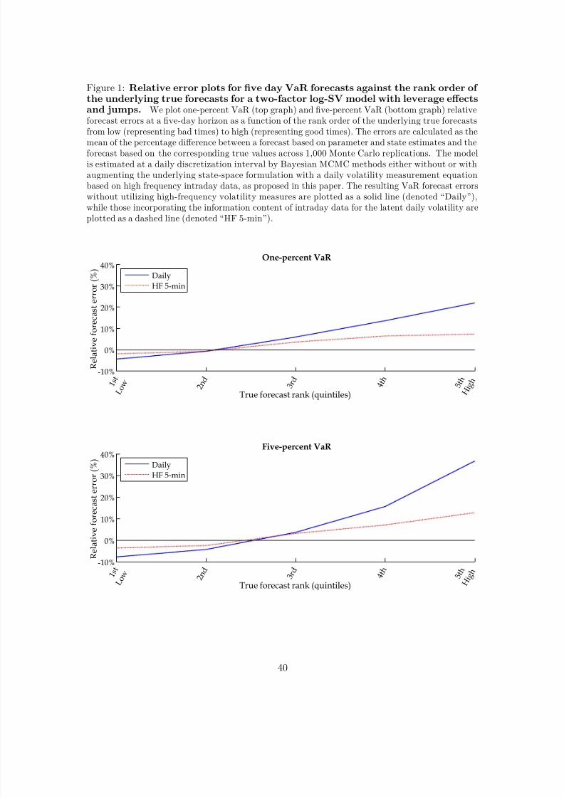
8/3/2019 The In Format In Content of High-Frequency Data for Estimating Equity Return Models
http://slidepdf.com/reader/full/the-in-format-in-content-of-high-frequency-data-for-estimating-equity-return 45/48
Figure 1: Relative error plots for five day VaR forecasts against the rank order of the underlying true forecasts for a two-factor log-SV model with leverage effectsand jumps. We plot one-percent VaR (top graph) and five-percent VaR (bottom graph) relativeforecast errors at a five-day horizon as a function of the rank order of the underlying true forecastsfrom low (representing bad times) to high (representing good times). The errors are calculated as themean of the percentage difference between a forecast based on parameter and state estimates and theforecast based on the corresponding true values across 1,000 Monte Carlo replications. The modelis estimated at a daily discretization interval by Bayesian MCMC methods either without or withaugmenting the underlying state-space formulation with a daily volatility measurement equationbased on high frequency intraday data, as proposed in this paper. The resulting VaR forecast errorswithout utilizing high-frequency volatility measures are plotted as a solid line (denoted “Daily”),while those incorporating the information content of intraday data for the latent daily volatility areplotted as a dashed line (denoted “HF 5-min”).
-10%
0%
10%
20%
30%
40%
True forecast rank (quintiles)
R e l a t i v e f o r e c a s t e r r o r ( %
)
One-percent VaR
1 s t
L o w 2 n
d 3 r
d 4 t h
5 t h
H i g h
DailyHF 5-min
-10%
0%
10%
20%
30%
40%
True forecast rank (quintiles)
R e l a t i v e f o r e c a s t e r r o r ( % )
Five-percent VaR
1 s t
L o w 2 n
d 3 r
d 4 t h
5 t h
H i g h
Daily
HF 5-min
40
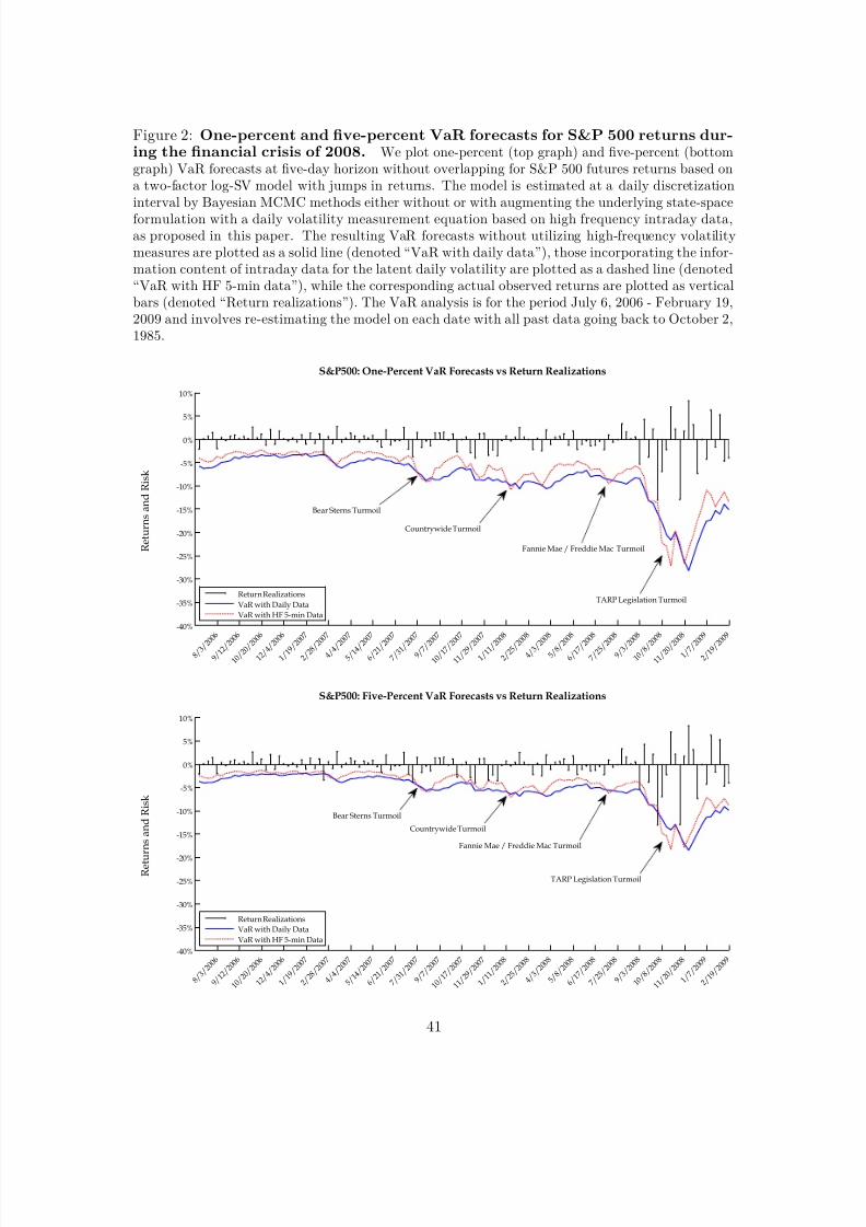
8/3/2019 The In Format In Content of High-Frequency Data for Estimating Equity Return Models
http://slidepdf.com/reader/full/the-in-format-in-content-of-high-frequency-data-for-estimating-equity-return 46/48
Figure 2: One-percent and five-percent VaR forecasts for S&P 500 returns dur-ing the financial crisis of 2008. We plot one-percent (top graph) and five-percent (bottomgraph) VaR forecasts at five-day horizon without overlapping for S&P 500 futures returns based ona two-factor log-SV model with jumps in returns. The model is estimated at a daily discretizationinterval by Bayesian MCMC methods either without or with augmenting the underlying state-spaceformulation with a daily volatility measurement equation based on high frequency intraday data,as proposed in this paper. The resulting VaR forecasts without utilizing high-frequency volatilitymeasures are plotted as a solid line (denoted “VaR with daily data”), those incorporating the infor-mation content of intraday data for the latent daily volatility are plotted as a dashed line (denoted“VaR with HF 5-min data”), while the corresponding actual observed returns are plotted as verticalbars (denoted “Return realizations”). The VaR analysis is for the period July 6, 2006 - February 19,2009 and involves re-estimating the model on each date with all past data going back to October 2,1985.
-40%
-35%
-30%
-25%
-20%
-15%
-10%
-5%
0%
5%
10%
R e t u r n s a n d
R i s k
S&P500: One-Percent VaR Forecasts vs Return Realizations
8 / 3 /
2 0 0 6
9 / 1 2
/ 2 0 0 6
1 0 / 2
0 / 2 0 0
6
1 2 / 4
/ 2 0 0 6
1 / 1 9
/ 2 0 0 7
2 / 2 8
/ 2 0 0 7
4 / 4 / 2 0 0
7
5 / 1 4
/ 2 0 0 7
6 / 2 1
/ 2 0 0 7
7 / 3 1
/ 2 0 0 7
9 / 7 /
2 0 0 7
1 0 / 1 7 /
2 0 0 7
1 1 / 2
9 / 2 0 0
7
1 / 1 1
/ 2 0 0 8
2 / 2 5
/ 2 0 0 8
4 / 3 /
2 0 0 8
5 / 8 / 2 0 0
8
6 / 1 7
/ 2 0 0 8
7 / 2 5
/ 2 0 0 8
9 / 3 /
2 0 0 8
1 0 / 8
/ 2 0 0 8
1 1 / 2
0 / 2 0 0
8
1 / 7 /
2 0 0 9
2 / 1 9
/ 2 0 0 9
Return Realizations
VaR with Daily Data
VaR with HF 5-min Data
Bear Sterns Turmoil
Countrywide Turmoil
Fannie Mae / Freddie Mac Turmoil
TARP Legislation Turmoil
-40%
-35%
-30%
-25%
-20%
-15%
-10%
-5%
0%
5%
10%
R e t u r
n s a n d
R i s k
S&P500: Five-Percent VaR Forecasts vs Return Realizations
8 / 3 /
2 0 0 6
9 / 1 2
/ 2 0 0 6
1 0 / 2
0 / 2 0
0 6
1 2 / 4
/ 2 0 0
6
1 / 1 9
/ 2 0 0 7
2 / 2 8
/ 2 0 0 7
4 / 4 / 2 0
0 7
5 / 1 4
/ 2 0 0 7
6 / 2 1
/ 2 0 0 7
7 / 3 1
/ 2 0 0 7
9 / 7 /
2 0 0 7
1 0 / 1 7 /
2 0 0 7
1 1 / 2
9 / 2 0
0 7
1 / 1 1
/ 2 0 0
8
2 / 2 5
/ 2 0 0
8
4 / 3 /
2 0 0 8
5 / 8 / 2 0
0 8
6 / 1 7
/ 2 0 0
8
7 / 2 5
/ 2 0 0
8
9 / 3 /
2 0 0 8
1 0 / 8
/ 2 0 0
8
1 1 / 2
0 / 2 0
0 8
1 / 7 /
2 0 0 9
2 / 1 9
/ 2 0 0
9
Return Realizations
VaR with Daily Data
VaR with HF 5-min Data
Bear Sterns Turmoil
Countrywide Turmoil
Fannie Mae / Freddie Mac Turmoil
TARP Legislation Turmoil
41
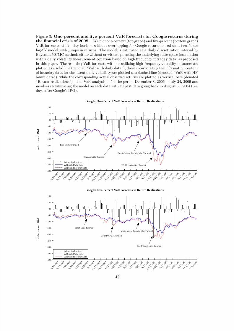
8/3/2019 The In Format In Content of High-Frequency Data for Estimating Equity Return Models
http://slidepdf.com/reader/full/the-in-format-in-content-of-high-frequency-data-for-estimating-equity-return 47/48
Figure 3: One-percent and five-percent VaR forecasts for Google returns duringthe financial crisis of 2008. We plot one-percent (top graph) and five-percent (bottom graph)VaR forecasts at five-day horizon without overlapping for Google returns based on a two-factorlog-SV model with jumps in returns. The model is estimated at a daily discretization interval byBayesian MCMC methods either without or with augmenting the underlying state-space formulationwith a daily volatility measurement equation based on high frequency intraday data, as proposedin this paper. The resulting VaR forecasts without utilizing high-frequency volatility measures areplotted as a solid line (denoted “VaR with daily data”), those incorporating the information contentof intraday data for the latent daily volatility are plotted as a dashed line (denoted “VaR with HF5-min data”), while the corresponding actual observed returns are plotted as vertical bars (denoted“Return realizations”). The VaR analysis is for the period December 8, 2006 - July 24, 2009 andinvolves re-estimating the model on each date with all past data going back to August 30, 2004 (tendays after Google’s IPO).
-40%
-35%
-30%
-25%
-20%
-15%
-10%
-5%
0%
5%
10%
R e t u r n s a n d
R i s k
Google: One-Percent VaR Forecasts vs Return Realizations
1 / 1 8
/ 2 0 0 7
2 / 2 7
/ 2 0 0 7
4 / 4 / 2 0
0 7
5 / 1 4
/ 2 0 0 7
6 / 2 1
/ 2 0 0 7
7 / 3 1
/ 2 0 0 7
9 / 7 /
2 0 0 7
1 0 / 1 7 /
2 0 0 7
1 1 / 2
9 / 2 0
0 7
1 / 1 1
/ 2 0 0 8
2 / 2 5
/ 2 0 0
8
4 / 3 /
2 0 0 8
5 / 8 / 2 0
0 8
6 / 1 7
/ 2 0 0 8
7 / 2 5
/ 2 0 0 8
9 / 3 /
2 0 0 8
1 0 / 1 5 /
2 0 0 8
1 1 / 2
4 / 2 0
0 8
1 / 9 / 2 0
0 9
2 / 2 3
/ 2 0 0
9
3 / 3 0
/ 2 0 0
9
5 / 7 /
2 0 0 9
6 / 1 6
/ 2 0 0 9
7 / 2 4
/ 2 0 0 9
Return Realizations
VaR with Daily Data
VaR with HF 5-min Data
Bear Sterns Turmoil
Countrywide Turmoil
Fannie Mae / Freddie Mac Turmoil
TARP Legislation Turmoil
-40%
-35%
-30%
-25%
-20%
-15%
-10%
-5%
0%
5%
10%
R e t u r n s
a n d
R i s k
Google: Five-Percent VaR Forecasts vs Return Realizations
1 / 1 8
/ 2 0 0 7
2 / 2 7
/ 2 0 0 7
4 / 4 / 2 0
0 7
5 / 1 4
/ 2 0 0 7
6 / 2 1
/ 2 0 0 7
7 / 3 1
/ 2 0 0 7
9 / 7 /
2 0 0 7
1 0 / 1 7 /
2 0 0 7
1 1 / 2
9 / 2 0
0 7
1 / 1 1
/ 2 0 0 8
2 / 2 5
/ 2 0 0
8
4 / 3 /
2 0 0 8
5 / 8 / 2 0
0 8
6 / 1 7
/ 2 0 0 8
7 / 2 5
/ 2 0 0 8
9 / 3 /
2 0 0 8
1 0 / 1 5 /
2 0 0 8
1 1 / 2
4 / 2 0
0 8
1 / 9 / 2 0
0 9
2 / 2 3
/ 2 0 0
9
3 / 3 0
/ 2 0 0
9
5 / 7 /
2 0 0 9
6 / 1 6
/ 2 0 0 9
7 / 2 4
/ 2 0 0 9
Return Realizations
VaR with Daily Data
VaR with HF 5-min Data
Bear Sterns Turmoil
Countrywide Turmoil
Fannie Mae / Freddie Mac Turmoil
TARP Legislation Turmoil
42

8/3/2019 The In Format In Content of High-Frequency Data for Estimating Equity Return Models
http://slidepdf.com/reader/full/the-in-format-in-content-of-high-frequency-data-for-estimating-equity-return 48/48
Finance and Economics Discussion Series
Divisions of Research & Statistics and Monetary Affairs
Federal Reserve Board, Washington, D.C.
Starting with working papers in 1996, electronic copies of FEDS papers
may be downloaded at the
Internet site: http://www.federalreserve.gov/pubs/feds
Single hard copies of FEDS papers may be obtained by request from:
Diane Linder
Finance and Economics Discussion Series
Mailstop 80
Federal Reserve Board
Washington, D.C. 20551
FAX: (202) [email protected]
Comments about the FEDS working paper series may be addressed to:
Michael Palumbo
Finance and Economics Discussion Series
Mailstop 61
Federal Reserve Board
Washington, D.C. 20551