estimating the nonlinear resonant frequency of a single

ARTICLE IN PRESS

Contents lists available at ScienceDirect

Journal of Sound and Vibration

Journal of Sound and Vibration 329 (2010) 1137–1153

0022-46

doi:10.1

� Tel.

E-m1 Se

journal homepage: www.elsevier.com/locate/jsvi

Estimating the nonlinear resonant frequency of a singlepile in nonlinear soil

Nicholas Andrew Alexander �,1

Department of Civil Engineering, University of Bristol, UK

a r t i c l e i n f o

Article history:

Received 18 February 2008

Received in revised form

21 October 2009

Accepted 21 October 2009

Handling Editor: M.P. Cartmelldependent is considered. A non-dimensional equation of motion for the system

Available online 13 November 2009

0X/$ - see front matter & 2009 Elsevier Ltd. A

016/j.jsv.2009.10.026

: þ0117 928 8687.

ail addresses: [email protected], dr

nior Lecturer in Structural Engineering.

a b s t r a c t

Analytical expressions are determined for the nonlinear resonant frequency (or natural

frequency) of the fundamental lateral mode of a pile. A pile with a floating toe, with and

without pile cap is considered in this paper. The influence of a nonlinear soil spring

model that varies with depth and a nonlinear damping model that is strain amplitude

dynamics is derived from an energy based formulation. This equation is a Duffing’s type

nonlinear differential system that has nonlinear damping. Harmonic balance with

numerical continuation is employed to determine the nonlinear resonance curves of the

system. Comparison with some experimental results is made.

& 2009 Elsevier Ltd. All rights reserved.

1. Introduction

Climate change has resulted in a change in societal requirements for energy production. The need for reduced CO2

emissions and the perceived threats to the supply of carbon based energy sources has resulted in a return to renewableenergy. For example, there has been a huge increase in wind energy production. Vast wind farms have been constructedboth on- and off-shore. The off-shore wind turbines use a range of different types of foundations that are dependant on siteconditions. Use of large monopile foundations is not uncommon. Efficient design requires simple design rules as well ascomplex computational modelling. Nonlinear finite element modelling of time varying loading histories, such asearthquakes, is a complex undertaking for a design engineer. Validation of results obtained by such a process is vital. Sosimple design formulae are very useful in practice. Thus, there is a need to develop good approximations to the nonlinearresonant frequency of piles in both linear and nonlinear soils.

It is surprising that, in the literature, there is no exact analytic expression for the natural frequency of a single pile inelastic medium. In the linear case, and constant soil stiffness with depth, researchers [1–4] suggest various semi-analytical/empirical expressions based on a simple equivalent cantilever system. Ref. [1] provides a method for obtaining ananalytically accurate equivalent stiffness and mass of the pile that is based on linear soil. For the case of nonlinear soil nosuch resonant frequency estimates are available.

This paper considers a single pile, with an additional lumped mass at its head. It is embedded in a nonlinear soil. Thelinear natural frequency is estimated and in addition the nonlinear resonant frequency is obtained. This is for the case ofnonlinear soil behaviour.

This paper uses a soil springs analogy (after Winkler) to model the soil. Nonlinear P–y curves (where P is spring load perunit length and y is lateral pile deflection) are employed to determine the spring stiffness vs. compression of these springs.

ll rights reserved.

[email protected].

www.elsevier.com/locate/jsvi

dx.doi.org/10.1016/j.jsv.2009.10.026

mailto:[email protected]

mailto:[email protected]

ARTICLE IN PRESS

Nomenclature2

ai harmonic balance coefficientsag peak ground acceleration (PGA) ðLÞðTÞ�2

A ground acceleration amplitudec; c1; c2 Rayleigh damping coefficient ðFÞðTÞðLÞ�2

C1;C2 linear and nonlinear damping coefficientsD dynamic matrix for linear modal analysisD pile diameter ðLÞEI pile flexural rigidity ðFÞðLÞ2

F forcing parameterk0 initial modulus of subgrade reaction ðFÞðLÞ�3

kw1 linear soil spring constants ðFÞðLÞ�2

kw2 nonlinear soil spring constant ðFÞðLÞ�4

K stiffness matrix for linear modal analysisK1 linear stiffness coefficient of systemK2 nonlinear stiffness coefficient of systemKg linear stiffness coefficient of near–far-field

boundaryL total pile length ðLÞmh mass of at head of pile ðFÞðTÞ2ðLÞ�1

mp mass per unit length of pile ðFÞðTÞ2ðLÞ�2

m mass per unit length of pile and near field soillayer ðFÞðTÞ2ðLÞ�2

M total system massM mass matrix for linear modal analysisMg effective mass at near–far-field boundaryP soil spring load per unit length ðFÞðLÞ�1

p soil spring load per unit area ðFÞðLÞ�2

Pu ultimate bearing capacity at depth z ðFÞðLÞ�1

Pub ultimate bearing capacity at base (toe) of pileðFÞðLÞ�1

qi solution vector of harmonic balance continua-tion.

R Rayleigh dissipative function ðFÞðTÞ�1ðLÞ

s frequency, dimensional ðradÞðTÞ�1

t time ðTÞu scaled ordinate w

ug scaled ordinate wg

U total potential energy ðFÞðLÞ

T total kinetic energy ðFÞðLÞwðtÞ temporal ordinate of y

wgðtÞ temporal ordinate of yg

wq;w vectors of generalised coordinates, for linearmodal analysis

y relative lateral pile deflection ðLÞyg displacements of the near–far field boundary

ðLÞ

yp limit of deflection for problem domain ðLÞz ordinate along the pile ðLÞa mass ratiob1 nonlinear to linear stiffness ratio of systemb2 mass ratio of far-field effective mass to pile

and near-field massb3 stiffness ratio of near–far-field boundary to

pile and near-field stiffnesse strain in soil springszbD breadth (out of plane) soil layer ðLÞzwL effective, in-plane, width of near-field soil

layer ðLÞZ1 linear soil to pile stiffness parameterZ2 nonlinear soil to pile stiffness parameterh1; h2 vectors of shifted Legendre polynomials, for

linear modal analysism1 linear damping ratiom2 nonlinear damping ratiomn nonlinear to linear damping parameter ratiommax maximum ratio of critical damping at large soil

strainx ordinate along pileP Lagrangian for linear modal analysis ðFÞðLÞrs density of near-field soil layer ðFÞðTÞ2ðLÞ�4

t scaled timefðxÞ spatial ordinate of y, shape functioncðxÞ spatial ordinate of yg , shape functiono forcing frequency ratioof forcing frequency ðradÞðTÞ�1

o1 small-strain (linear) resonant fundamentalfrequency of system ðradÞðTÞ�1

N.A. Alexander / Journal of Sound and Vibration 329 (2010) 1137–11531138

The stiffness of these springs also varies with depth from the surface. In addition, a strain-dependant nonlinear dampingfunction is employed. Both the stiffness and damping functions match experimental observations qualitatively. Aftervarious non-dimensional ordinates are introduced, it is possible to reduce the general system to Duffing’s oscillator thathas nonlinear damping. It is demonstrated that this Duffing’s like system is a generic one that applies for all cases ofdifferent pile kinematical boundary conditions.

Three main results are presented in this paper, (i) the small strain (linear) resonant system frequency o1, Fig. 2 (or Eq. (61)),(ii) the reduction of this linear frequency with increases in non-dimensional forcing parameter F, Eq. (45) and (iii) therelationship between non-dimensional forcing F and peak ground acceleration (PGA) ag , Eq. (51). Experimental results obtainedelsewhere together with a finite element analysis (FEA) are employed to provide some validation of the small strain formula.

2. Analytical model

Consider the system described in Fig. 1. The pile is surrounded by a ‘‘near field’’ soil stack of layers. A continuum oflayers surround the pile. Each layer contains a nonlinear spring, nonlinear dashpot and lumped masses. The effective width

2 Dimensional units denoted in this paper by bracketed terms, where (F) is force, (L) is length and (T) is time. The dimensionless derived unit (rad) is

an angle in radians.

ARTICLE IN PRESS

Far field yg (z,t)

Near field

LSoil layer

z

zδ

Far field Reaction Q (z,t)δ mh0 y

Nonlinear Spring

Nonlinear damper

Lumped masses

y

yg

z

y(z,t) + wς L

Fig. 1. Analytical model.

N.A. Alexander / Journal of Sound and Vibration 329 (2010) 1137–1153 1139

of the near-field layer is zwL. The system is sub-structured such that only the near field soil, pile and superstructure massare considered. For equilibrium to be maintained a set of reactions, Q ðz; tÞ, that vary with depth are applied to the near fieldsoil stack. Thus, only the horizontal displacement at the far field–near field interface ygðz; tÞ and these reactions Q ðz; tÞ arenecessary. The total displacement of the pile is ygðz; tÞ þ yðz; tÞ where yðz; tÞ is a relative horizontal displacement of the pile.

2.1. Using P–y backbone curves

For a range of different soils many different P–y curves proposed by researchers [2–7] and others (too numerous tomention here). The fidelity of these forms of curves to experimental data has been questioned by [7,8]. Results suggest thatthere is some scatter about these nonlinear trends. This scatter is due to lack of heterogeneity and complex hystereticnonlinear behaviour of real soils. An example of this scatter is given in [9,10]; where full scale dynamic test data for a piledriven in medium-dense sand is obtained. Dynamic test results show an approximately cubic p–y curve (where p is soilspring load per unit area) complete with a falling part, (cf. Fig. 12 in [9]).

Note that P–y curves for pile-soil springs are normally obtained by applying a load at the head of the pile and recordingthe displacements of the pile. This is the case for experimental study [9,10]. In this situation the pile ground displacementfield yg is zero and y is the relative displacement of pile and the total displacement of the pile.

More recent work, [11], has suggested that the p–y curves can be loading rate dependant. Thus [11] suggest p–y curvesbased on static or slow cyclic loading may underestimate the backbone observed under faster cyclic loading. This strainrate hardening in clay soils is clear; in sands this effect seems less marked. The basic shape of these dynamic p–y curves, in[11], is still fairly similar to the static p–y curves with a scaling (stretching) of the p axis.

However, for all their limitations P–y curves provide a pragmatic and useful engineering simplification and are usedwidely in practice. In this paper the form of [7,12] is taken. This is shown in Eq. (1); where P is the soil-spring reaction atdepth z, Pu is the ultimate bearing capacity at a depth of z, A is 0.9 a reduction factor for dynamics, k0 is the initial modulusof subgrade reaction [6], y is the horizontal pile deflection at depth z. This can be re-expressed by assuming that the Pu

varies linearly with depth (2); thus it can be expressed in terms of Pub the ultimate bearing capacity at the base of the pilei.e. at depth L. This follows the functional form presented in work of [13–16]. This linear assumption differs from theAmerican Petroleum Institute (API) [12] recommendation that assumes a quadratic variation of Pu with depth for ‘‘shallowdepths’’ and a linear variation of Pu with depth for ‘‘deep depths’’. Ref. [16] suggests that the API quadratic variation thatwas based on a wedge failure mechanism at shallow depths is unduly optimistic compared with other proposed models.Experimental results presented in [17] (cf. Figs. 12 and 14) show a near linearly increase in Pu with depth. Nevertheless, inthis paper, a linear variation with depth is assumed mainly because it is computationally simplifying.

Pðx; zÞ ¼ seAPutanhk0z

APuy

� �¼ seAPub

z

L

� �tanh

k0L

APuby

� �(1)

Pu ¼ Pubz

L

� �(2)

For dynamic p–y curves to be incorporated, as [11] suggests, a scale factor se to the p axis should be applied. A Taylor seriesexpansion suggests that the tanh function can be expressed as a cubic with higher terms neglected, for a small range of y.However, just expanding and neglecting higher order terms does not often produce the best fit over the problem domainjyjryp. The optimal values of linear and nonlinear spring constants kw1 and kw2 should be sought, in a least square sense,employing Eq. (60) from Appendix B. Thus, the optimal spring coefficients are given by (4) and (5) in terms of k0, L, yp andPub. Note that for jyj4yp the cubic function falls away from API backbone curve. This can be an advantage as it modelsdegradation of stiffness at large cyclic strains as seen in [9].

ARTICLE IN PRESS


In summary, the cubic P–y curve proposed in this paper enforces quartic nonlinear strain energy of the soil.

L

z

� �P ¼ seAPubtanh

k0L

APuby

� �� kw1y� kw2y3 þ Oðy5Þ; jyjryp (3)

kw1 ¼75

4y3p

Z yp

0

L

z

� �Py dy�

105

4y5p

Z yp

0

L

z

� �Py3 dy (4)

kw2 ¼105

4y5p

Z yp

0

L

z

� �Py dy�

175

4y7p

Z yp

0

L

z

� �Py3 dy (5)

2.2. Potential energy of system

The potential Energy U of this system is composed of two terms: (i) the flexural strain energy of the pile group and (ii)the soil spring stiffness energy. The work done by the far-field soil reactions Q is neglected here as it does not contribute tothe subsequent equations of motion. Hysteretic behaviour of springs is not modelled directly as this greatly increases theanalytical complexity. However, it is not ignored. The hysteretic behaviour of springs is summed up per cycle and includedas an increased nonlinear damping term proposed later. This approach follows work of Voigt and Maxwell described in[18]. This approach is used to determine the variation of soil damping coefficient with strain levels.

U ¼1

2

Z L

0EIðy00 þ yg

00 Þ2 dzþ

Z L

0

1

2kw1

z

L

� �y2 �

1

4kw2

z

L

� �y4 dz (6)

If a classical Rayleigh–Ritz spatial–temporal series is adopted, i.e. y ¼P

wiðtÞfiðzÞ then an n degree of freedom nonlinearsystem is obtained. This is equivalent to a high order (i.e. 2n) nonlinear ODE. Unfortunately, this is not suitable for an initialinvestigation into the problem. These high order systems are left for later. In this paper, a first order approximation(a reduced order system) is assumed e.g. using Eq. (7) that result in a nonlinear, single degree of freedom system. Thisintroduces one unknown degree of freedom, w, where wL is the displacement at the top of the pile, and the known degreeof freedom, wg where wgL is the surface ground horizontal displacement. A non-dimensional variable, x, is introduced; it isan ordinate along the pile. Hence primes and double primed variables from now on denote first and second derivative withrespect to x. The potential energy can be re-expressed as (8): non-dimensional parameters in Eqs. (9) and (10) areintroduced.

y ¼ LwðtÞfðxÞ; yg ¼ LwgðtÞcðxÞ; x ¼ z=L (7)

U ¼1

2

EI

LðK1w2 �

1

2K2w4 þ 2KgwwgÞ þ OðwgÞ (8)

Z1 ¼kw1L4

EI; Z2 ¼

kw2L6

EI(9)

K1 ¼

Z 1

0f002þ Z1xf

2 dx; K2 ¼ Z2

Z 1

0xf4 dx; Kg ¼

Z 1

0f00c00 dx (10)

2.3. Kinetic energy of system

The translational, horizontal, kinetic energy T of the system is defined in (12). The rotational kinetic energy of pile andsuperstructure mass are neglected in this paper. Parameter mh is the lumped mass at pile head; i.e. the mass of anystructure attached to the top of the pile. m is the mass per unit depth of the pile and soil layer; where mp is the mass perunit depth of the pile and rs density of the ‘‘near field’’ soil layer. The out of plain breadth of the soil layer is assumed to bezbD. The soil mass for a layer dz is lumped half on the pile and half at the near–far-field boundary. The kinetic energy can bere-expressed, in quadratic form, in terms of degrees of freedom w and wg by Eq. (13); by using non-dimensionalparameters in Eqs. (14) and (15).

m ¼ mp þ12rszwzbLD (11)

T ¼1

2

�mhð _ygð0Þ þ _yð0ÞÞ2 þm

Z L

0ð _yg þ _yÞ2 dz

�(12)

T ¼ 12mL3ðM _w2

þ 2Mg _w _wgÞ þ Oð _w2g Þ (13)

M ¼ afð0Þ2 þZ 1

0f2 dx; Mg ¼ afð0Þcð0Þ þ

Z 1

0fcdx (14)

a ¼ mh

mL(15)

ARTICLE IN PRESS


2.4. Rayleigh dissipative function of system

The damping coefficient of the soil is assumed quadratic in nature, (16); this follows the experimental evidence of [8,19]that suggest the ratio of critical damping is dependent of cyclic soil shear strain amplitude. The strain in the soil spring ise ¼ y=zwL. The system Rayleigh dissipative function, R, is given by Eq. (17); frequency s is introduced to aid latersimplifications.

c ¼ c1 þ c2e2 (16)

R ¼1

2

Z L

0c1 þ c2

y

zwL

� �2 !

_y2 dz ¼1

2mL3sðC1 þ C2w2Þ _w2 (17)

C1 ¼c1

ms

Z 1

0f2 dx; C2 ¼

c2

msz2w

Z 1

0f4 dx (18)

s2 ¼EI

mL4(19)

2.5. Equation of motion for system

Thus the Euler–Lagrange–Rayleigh equation of motion (20) can be obtained from (8), (13) and (17). This is re-expressedby the introduction of frequency parameter o1 Eq. (21). Also non-dimensional parameters b1, b2, b3, m1, m2 are introduced,see Eqs. (22) and (23)

€w þ 2ðm1 þ m2w2Þ _w þw� b1w3 ¼ �b2 €wg � b3wg (20)

o1 ¼ s

ffiffiffiffiffiffiK1

M

r(21)

b1 ¼K2

K1; b2 ¼

Mg

M; b3 ¼

Kg

K1(22)

m1 ¼C1

2ffiffiffiffiffiffiffiffiffiffiMK1

p ; m2 ¼C2

2ffiffiffiffiffiffiffiffiffiffiMK1

p (23)

This equation of motion (20) has been further simplified by introducing a time-scale t ¼ o1t. Note, subsequently, dotsabove letters denote differentials with respect to t i.e. _w ¼ dw=dt, €w ¼ d2w=dt2 and €wg ¼ d2wg=dt2.

One final further scaling simplifies this equation. The generalised ordinate w and ground displacement ordinate wg arere-scaled by (24). This results in Eq. (25), that is a Duffing’s [20–23] oscillator but with nonlinear damping.

w ¼ b�1=21 u; wg ¼ b�1=2

1 ug (24)

€u þ 2m1ð1þ mnu2Þ _u þ u� u3 ¼ �b2 €ug � b3ug (25)

mn ¼m2

m1b1

(26)

3. Solutions of nonlinear system

3.1. What form should the spatial shape function f take?

This is a difficult question to answer for a number of reasons. Firstly and fairly obviously, it should be stated that thecloser f is to the fundamental nonlinear mode shape, the more accurate this single degree of freedom model will be.Secondly, the relative stiffness of soil to pile governs this mode shape f. There is also the problem that if the reduction instiffness due to nonlinearity significantly influences this pile/soil spring stiffness ratio it will influence f. Hence theaccuracy of the simplified model is likely to reduce as response amplitude increases. Finally, the boundary conditions towhich the pile is subject govern the form of f significantly. The boundary conditions at the bottom (toe) of the pile aregoverned by the soil layer at this level. The boundary conditions at the top (head) are governed by the pile cap, etc.

So how about employing the systems first linear natural mode for f? This would represent a projection of the nonlinearsystem onto a truncated linear modal basis. It would give a very good approximation at low amplitudes. It would be usefulto observe how the soil/pile linear stiffness ratio, Z1, influences the linear fundamental natural mode f.

First let us compute an n degree of freedom estimate of the linear natural modes. A series of shifted Legendrepolynomials, Pn are used. These are defined to be orthogonal over range zero to one. The pile displacement y can be defined

ARTICLE IN PRESS


(28) in term of vector of shape functions h1 and h2 can be defined as (27). Essentially, the q generalised coordinates wq 2 Rq

will be constrained by the boundary conditions leaving n unconstrained generalised coordinates w 2 Rn.

hT1 ¼ ½Pnþq�1; Pnþq�2; . . . ; Pn� 2 R

q; hT2 ¼ ½Pn�1; Pn�3; . . .P0� 2 R

n (27)

y ¼ LðhT1wq þ hT

2wÞ (28)

For a pile without pile cap the boundary conditions are y00ð1Þ ¼ y000

ð1Þ ¼ 0; these are represented in Eq. (29). For the case of apile with pile cap a further boundary condition is included y0ð0Þ ¼ 0; these are represented in Eq. (30). Thus, the shapefunction vector / that satisfies these boundary conditions is given by (31). The only requirement for use of this result isthat the boundary condition block matrix A1 2 R

q�q should not be singular. In the case of singular A1 reordering theLegendre polynomials will normally help to obtain a non-singular A1. Note that re-ordering the rows or columns of generalmatrix A cannot change its rank but it can change the rank of a sub-matrix of A; and this is what is proposed here. Blockmatrix A2 2 R

q�n is generally not square. For clarity, Appendix A gives a worked example of Eqs. (29) and (31).

y00ð1ÞT1 y00ð1ÞT2y000

ð1ÞT1 y000

ð1ÞT2

" #wq

w

� �¼ ½A1 A2�

wq

w

� �¼ 0 (29)

y0ð0ÞT1 y0ð0ÞT2y00ð1ÞT1 y00ð1ÞT2y000

ð1ÞT1 y000

ð1ÞT2

2664

3775 wq

w

� �¼ ½A1 A2�

wq

w

� �¼ 0 (30)

y ¼ LwT/; / ¼ ðhT2 � hT

1A�11 A2Þ

T (31)

Note that this approach is more subtle than conventional finite element analysis (FEA). Here, the shape functions arecontinuous across the entire problem domain. This is more similar to boundary element method. Degrees of freedom (dofs)are amplitudes of shape functions here. This contrasts with FEA, where degrees of freedom are general displacements orrotations at nodal positions. Thus, in FEA, dofs at boundaries must be constrained to satisfy boundary conditions. Herehowever, dofs are shape function amplitudes, thus it is necessary and sufficient to constrain almost any q dofs; (with theproviso that these constrained dofs do not result in singular A1).

Given this series expansion for the pile displacement the Lagrangian P can be defined thus;

PmL3¼

1

2

�að _wT/ð0ÞÞ2 þ

Z 1

0ð _wT/Þ2 dx

��

1

2s2

Z 1

0ðwT/00Þ2 þ Z1xðw

T/Þ2 dx (32)

By employing the Euler–Lagrange equations to P the dynamic matrix D can be obtained; Eq. (34). The eigenvectors of D arethe natural linear modes of vibration of the pile–soil system.

K ¼

Z 1

0/00/

00Tþ Z1x//T dx; M ¼ a/ð0Þ/ð0ÞT þ

Z 1

0//T dx (33)

D ¼ s2M�1K (34)

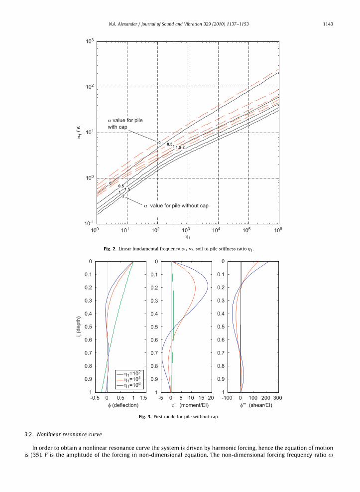
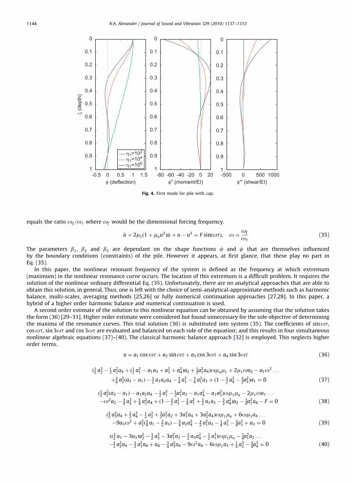
The first linear natural frequency o1 vs. parameters Z1 and a is displayed in Fig. 2. The first mode profile can be employedto determine moments and shear force functions. These functions are display graphically in Figs. 3 and 4. These momentdiagrams are very similar, qualitatively, to those obtained experimentally [8–10,19] and are consistent with othertheoretical work [24]. These conditions apply to case of homogeneous soil profile with depth. The presence of stiff soillayers at the pile base that are overlain with softer, more flexible, soil layers would suggest a different set of supportboundary conditions not considered here. Though, in principle, the approach would be the same with some smallmodifications for these different kinematic constraints.

A good analytical approximation to Fig. 2 is given in Appendices B–D, see Eq. (61). In addition a good approximation tothe linear first mode shape is presented. These formulae provide an alternative to employing Fig. 2 but are not used insubsequent analysis in this paper.

From these figures the influence of Z1 on the deflected shape is significant. However, for a given Z1, the reduction in soil-springs stiffness that is due to nonlinear behaviour of the soil changes the deflected shape a little. This is because only achange in the order of magnitude of Z1 effects the first mode shapes significantly. Thus, there is evidence to suggest, in thiscase, that the proposed single shape function (7) is a reasonable first approximation to the nonlinear natural mode. Inaddition, this is evidence that suggests the use of a single degree of freedom reduced order model is valid. The exact form ofthis shape function is obtained numerically by either eigenvalue analysis of matrix (34) or by using the very goodapproximation given in Appendices C–E.

ARTICLE IN PRESS

100 101 102 103 104 105 10610-1

100

101

102

103

0.51

1.5

2

η1

ω1

/ s

0 0.51 2

α value for pile without cap

α value for pilewith cap

1.5

0

Fig. 2. Linear fundamental frequency o1 vs. soil to pile stiffness ratio Z1.

-0.5 0 0.5 1 1.5

0

0.1

0.2

0.3

0.4

0.5

0.6

0.7

0.8

0.9

1

φ (deflection)

ξ (d

epth

)

-5 0 5 10 15 20

0

0.1

0.2

0.3

0.4

0.5

0.6

0.7

0.8

0.9

1

φ'' (moment/EI)-100 0 100 200 300

0

0.1

0.2

0.3

0.4

0.5

0.6

0.7

0.8

0.9

1

φ''' (shear/EI)

η1=102

η1=104

η1=106

Fig. 3. First mode for pile without cap.


3.2. Nonlinear resonance curve

In order to obtain a nonlinear resonance curve the system is driven by harmonic forcing, hence the equation of motionis (35). F is the amplitude of the forcing in non-dimensional equation. The non-dimensional forcing frequency ratio o

ARTICLE IN PRESS

-0.5 0 0.5 1 1.5

0

0.1

0.2

0.3

0.4

0.5

0.6

0.7

0.8

0.9

1

φ (deflection)

ξ (d

epth

)

-80 -60 -40 -20 0 20

0

0.1

0.2

0.3

0.4

0.5

0.6

0.7

0.8

0.9

1

φ'' (moment/EI)-500 0 500 1000

0

0.1

0.2

0.3

0.4

0.5

0.6

0.7

0.8

0.9

1

φ''' (shear/EI)

η1=102

η1=104

η1=106

Fig. 4. First mode for pile with cap.


equals the ratio of =o1 where of would be the dimensional forcing frequency.

€u þ 2m1ð1þ mnu2Þ _u þ u� u3 ¼ F sinðotÞ; o ¼of

o1(35)

The parameters b1, b2 and b3 are dependant on the shape functions f and c that are themselves influencedby the boundary conditions (constraints) of the pile. However it appears, at first glance, that these play no part inEq. (35).

In this paper, the nonlinear resonant frequency of the system is defined as the frequency at which extremum(maximum) in the nonlinear resonance curve occurs. The location of this extremum is a difficult problem. It requires thesolution of the nonlinear ordinary differential Eq. (35). Unfortunately, there are no analytical approaches that are able toobtain this solution, in general. Thus, one is left with the choice of semi-analytical-approximate methods such as harmonicbalance, multi-scales, averaging methods [25,26] or fully numerical continuation approaches [27,28]. In this paper, ahybrid of a higher order harmonic balance and numerical continuation is used.

A second order estimate of the solution to this nonlinear equation can be obtained by assuming that the solution takesthe form (36) [29–31]. Higher order estimate were considered but found unnecessary for the sole objective of determiningthe maxima of the resonance curves. This trial solution (36) is substituted into system (35). The coefficients of sinot,cosot, sin 3ot and cos 3ot are evaluated and balanced on each side of the equation; and this results in four simultaneousnonlinear algebraic equations (37)–(40). The classical harmonic balance approach [32] is employed. This neglects higherorder terms.

u ¼ a1 cosotþ a2 sinotþ a3 cos 3otþ a4 sin 3ot (36)

ð12 a32 �

12 a2

2a4 þ ð12 a2

1 � a1a3 þ a23 þ a2

4Þa2 þ12a2

1a4Þomnm1 þ 2m1oa2 � a1o2 . . .

þ34 a2

2ða3 � a1Þ �32 a1a2a4 �

34 a3

1 �34 a2

1a3 þ ð1�32 a2

4 �32a2

3Þa1 ¼ 0 (37)

ð12 a22ða3 � a1Þ � a1a2a4 �

12 a3

1 �12a2

1a3 � a1a24 � a1a2

3Þom1mn � 2m1oa1 . . .

�o2a2 �34 a3

2 þ34 a2

2a4 þ ð1�32 a2

3 �34 a2

1 þ32 a1a3 �

32 a2

4Þa2 �34a2

1a4 � F ¼ 0 (38)

ð32 a23a4 þ

32 a3

4 �12 a3

2 þ32a2

1a2 þ 3a21a4 þ 3a2

2a4Þom1mn þ 6om1a4 . . .

�9a3o2 þ a22ð

34 a1 �

32 a3Þ �

34 a3a2

4 �32 a2

1a3 �14 a3

1 �34a3

3 þ a3 ¼ 0 (39)

ðð32 a1 � 3a3Þa22 �

32 a3

3 � 3a21a3 �

32 a3a2

4 �12 a3

1Þom1mn �34a2

1a2 . . .

�32 a2

2a4 �32 a2

1a4 þ a4 �34 a2

3a4 � 9o2a4 � 6om1a3 þ14 a3

2 �34a3

4 ¼ 0 (40)

ARTICLE IN PRESS


The solution of Eqs. (37)–(40) required a numerical procedure, such as Gauss–Newton ([33], function fsolve). However,while a single solution to these equations is straightforward (with the correct numerical toolbox) the process of obtaining anonlinear resonance curve does require the addition of an arc-length continuation condition. Eq. (41) is a linear predictorbased on initial point on a path qi ¼ ½a1; a2; a3; a4;o�T, step size D and an normalised path vectordqi ¼ ½da1; da2; da3; da4; do�T. Vector ~q iþ1 represents the first estimate of the next point along the continued path.Eq. (42) is solved together with Eqs. (37)–(40); it ensures that solution must be normal to the path vector dqi. Essentiallythese equations act as a correction to the prediction (41). Once a solution is obtained this becomes the new qiþ1. An updateof the vector is made dqiþ1 based on linear extrapolation of the previous points qiþ1 and qi (43).

~q iþ1 ¼ qi þDdqi (41)

ðqi � ~q iþ1ÞTdqi ¼ 0 (42)

dqiþ1 ¼ðqiþ1 � qiÞ

Jqiþ1 � qiJ2(43)

3.2.1. Values for strain dependant ratio of critical damping

In order to solve these harmonic balance equation damping parameters m1 and mn must be specified. A significantamount of experimental work [34–37] and others has been performed on soils in order to determine the relationshipbetween damping ratio and cyclic shear strain amplitude. Most soils have a damping ratio of 0.01–0.02 at low strainlevels (of the order of 10�5) this grows approximately quadratically to about 0.15–0.25 at larger strain levels(of the order of 10�2).

In theory it is possible to work from Eq. (18) and (23) to determine m1 and mn. However, a set of parameters need to beassigned and these require, critically, knowledge of the width of the near-field zone zw and this is not well defined atpresent. In addition mode shape f is required. This suggests that pile boundary conditions would influence the dampingparameters in (35). However, it would be beneficial to keep (35) independent of f as far as possible.

So an alternative approach is sought. Note that the normalised cubic stiffness term of (35) is bounded physically byjujr1. Exceeding this limit is considered failure of the soil. Further investigations into velocity bounds of the catchmentbasins can be made by applying techniques in [38,39]. Thus, it is assumed that the maximum damping of the soil isachieved at this maximum displacement. It is assumed that at this level of normalised deformation that the systemdamping reaches mmax. Thus, the nonlinear damping parameter mn is defined by (44).

mn ¼mmax

m1

� 1 (44)

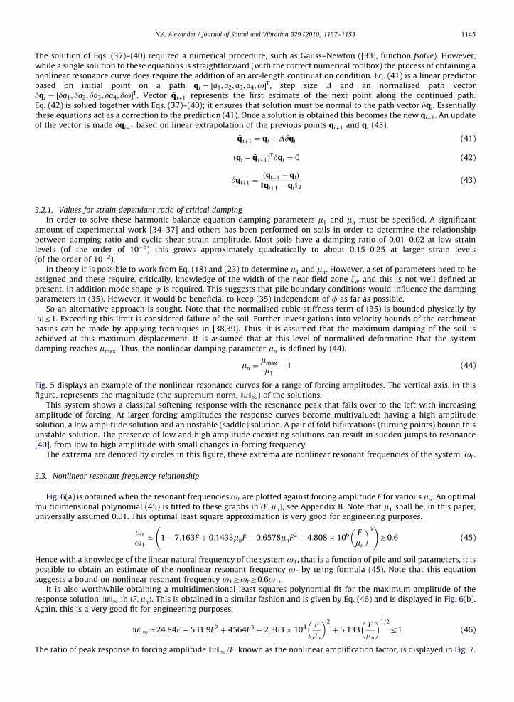
Fig. 5 displays an example of the nonlinear resonance curves for a range of forcing amplitudes. The vertical axis, in thisfigure, represents the magnitude (the supremum norm, JuJ1) of the solutions.

This system shows a classical softening response with the resonance peak that falls over to the left with increasingamplitude of forcing. At larger forcing amplitudes the response curves become multivalued; having a high amplitudesolution, a low amplitude solution and an unstable (saddle) solution. A pair of fold bifurcations (turning points) bound thisunstable solution. The presence of low and high amplitude coexisting solutions can result in sudden jumps to resonance[40], from low to high amplitude with small changes in forcing frequency.

The extrema are denoted by circles in this figure, these extrema are nonlinear resonant frequencies of the system, or .

3.3. Nonlinear resonant frequency relationship

Fig. 6(a) is obtained when the resonant frequencies or are plotted against forcing amplitude F for various mn. An optimalmultidimensional polynomial (45) is fitted to these graphs in ðF;mnÞ, see Appendix B. Note that m1 shall be, in this paper,universally assumed 0.01. This optimal least square approximation is very good for engineering purposes.

or

o1C 1� 7:163F þ 0:1433mnF � 0:6578mnF2 � 4:808� 106 F

mn

� �3 !

Z0:6 (45)

Hence with a knowledge of the linear natural frequency of the system o1, that is a function of pile and soil parameters, it ispossible to obtain an estimate of the nonlinear resonant frequency or by using formula (45). Note that this equationsuggests a bound on nonlinear resonant frequency o1ZorZ0:6o1.

It is also worthwhile obtaining a multidimensional least squares polynomial fit for the maximum amplitude of theresponse solution JuJ1 in ðF;mnÞ. This is obtained in a similar fashion and is given by Eq. (46) and is displayed in Fig. 6(b).Again, this is a very good fit for engineering purposes.

JuJ1C24:84F � 531:9F2 þ 4564F3 þ 2:363� 104 F

mn

� �2

þ 5:133F

mn

� �1=2

r1 (46)

The ratio of peak response to forcing amplitude JuJ1=F, known as the nonlinear amplification factor, is displayed in Fig. 7.

ARTICLE IN PRESS

0.5 0.6 0.7 0.8 0.9 1 1.10

0.1

0.2

0.3

0.4

0.5

0.6

0.7

0.8

0.9

1

ω

||u|| ∞

μ1=1%μmax=10%

Fig. 5. Example of nonlinear resonance curves.

0 0.01 0.02 0.03 0.04 0.05 0.06 0.07

R2=0.99696

F

ωr /

ω1

0 0.01 0.02 0.03 0.04 0.05 0.06 0.07

0.6

0.7

0.8

0.9

1

1.1

0

0.2

0.4

0.6

0.8

1R2=0.99713

F

||u|| ∞

25%μmax= 10%

25%16%13%μmax = 10% 19% 22%

Fig. 6. (a) Variation of nonlinear resonant frequency with forcing amplitude F and (b) variation in the maximum response of solution with F. In both cases

ðm1 ¼ 1%Þ.


3.4. Relating non-dimensional forcing amplitude F to far-field PGA

The key result, hitherto, is Eq. (45). From this the nonlinear resonant frequency can be determined in terms of the linear(very small soil-strain) fundamental natural frequency o1. This linear frequency o1 can be read from Fig. 2 (or Eq. (61)) forvarious mass ratios a and linear soil/pile stiffness ratios Z1. Hence, with (45) and Fig. 2 (or Eq. (61)) it is possible todetermine the nonlinear resonant frequency of the pile-soil system in terms of parameters (i) mass ratio a, (ii) linear soil topile stiffness Z1, (iii) frequency s, (iv) large strain damping mn and (v) non-dimensional forcing amplitude F.

ARTICLE IN PRESS

0 0.01 0.02 0.03 0.04 0.05 0.06 0.070

20

40

60

80100

120

140160

180

200

10% 13% 16% 19% 22% 25%

F

Am

plifi

catio

n Fa

ctor

|| u

||∞ /

Fμmax

Fig. 7. Nonlinear amplification factor for system.


Note, however, F is not a natural parameter; so it would be beneficial, for the practicing engineer, to express this interms of some dimensional quantity. By considering Eqs. (35) and (25) it is clear that the forcing function adopted in thestudy thus far is equivalent to a ground motion ug that can be obtained by equating these equations. Scaled ground motionwg and far-field ground motion €ygðx; tÞ can subsequently be determined by using (7) in terms of F, thus

€ygðx; tÞ ¼ o21L

o2F

b1=21 ðb2o2 � b3Þ

sin ðof tÞcðxÞ (47)

Hence, given a surface far-field peak ground acceleration (PGA) of ag ¼ maxð €ygð1; tÞÞ, the correspondent value of non-dimensional forcing amplitude F, at resonance, is given by (48).

F ¼ag

o21L

!A; A ¼ b1=2

1 b2 � b3

o1

or

� �2 !

(48)

So, clearly, one final equation is also required; an expression for A in terms of system parameters Z1, Z2 and a.The system non-dimensional parameters b2 and b3 can be evaluated in terms of parameters a and Z1 by using Eqs. (22),

(9), (10), (14) and (15). An estimate of the far-field ground displacement function c is required. In this paper a linearfunction is assumed, Eq. (49).

c ¼ 1� x (49)

Richart et al. [41] derived theoretical estimates for the variation in amplitude with depth for both seismic Rayleigh andLove waves. While these relationships are generally nonlinear, they are linear in the very shallow superficial layers of soilin which the pile is embedded. Hence, linear (49) is reasonable.

Therefore, in this case, Eq. (48) can expressed as the following Eq. (50).

A ¼ Z1=22 f ðZ1;aÞ; f ðZ1;aÞ ¼

R 10 xf4 dxR 1

0 f002þ Z1xf

2 dx

!1=2aþ

R 10 fcdx

aþR 1

0 f2 dx

!(50)

a has a second order influence; and this is born out by numerical investigations. By employing a least square fit that isreasonably good, R2 ¼ 0:98, the following expression is obtained (51). The coefficient b0 for this regression is (i) b0 ¼ 1:851(pile with cap) and (ii) b0 ¼ 1:731 (for pile without cap).

F ¼ b0ag

o21L

! ffiffiffiffiffiffiZ2

Z1

r(51)

4. Comparison with experimental centrifuge results [9,10]

4.1. Comparison with linear experimental results

It is important to ensure that the formulae presented are of the right order. Researchers [42–45] present interestingexperimental work on various failure mechanisms of piled structures. Experimental evidence is also available in theliterature for determining the linear resonance frequency. Work presented in [9,10] describes both full scale and centrifugestudies on the cyclic dynamic lateral pile behaviour in a cohesionless soil. These tests result provide information necessaryas an initial validation of the linear resonant frequency o1. From the test data, API curves can be estimated using the

ARTICLE IN PRESS

0 0.005 0.01 0.015 0.02 0.025 0.03 0.035 0.040

1000

2000

3000

4000

5000

6000

7000

8000

9000

10000

y [m]

P a

t (to

e of

pile

) [kN

/m]

yp

API for D5Fx

API for D10Fx

API for D16Fx

Fig. 8. Comparison of API curves for experimental data and cubic least square estimate of API using Eqs. (3)–(5).

Table 1Comparison of experimental, theoretical and FEA estimates of natural frequency.

Ting et al. [9,10] Back analysis from experimental dataþEq. (60) FEA

Test series o1=2p ðHzÞ kw1 ðkN m�2Þ kw2 ðkN m�4Þ Z1 ð2Þ Z2 ð2Þ a (–) o1=2p ðHzÞ o1=2p ðHzÞ

D5Fx 1.63 4.27E5 3.19E8 3.64E4 3.34E9 0.018 1.8 1.77

D10Fx 2.13 4.99E5 3.49E8 6.57E4 7.64E9 0.021 2.0 1.84

D16Fx 1.56 1.99E5 2.41E8 3.18E5 7.37E9 0.017 1.5 1.61


relative density of the sand. Fig. 8 show these P–y curves for the toe of the pile, for three data sets presented in [9]. Eqs. (4)and (5) are employed to determine the spring constants kw1 and kw2. These allow a back calculation of soil/pile stiffnessparameters Z1 and Z2. These are displayed in Table 1. A graphical comparison of the frequency estimates is displayed inFig. 9. Parameters zw and zb are required to evaluate the soil mass contribution to the dynamics of the pile. Model updatingwas employed to determine a best value of zwzb which as about 22. If zb ¼ 2, that out-of-plane breath is two diameters,then the in-plane width of the near field is 11 diameters; or 5.5 diameters on both sides of the pile. The interaction effectsbetween multiple piles, is thought to be negligible at about 6 diameters [46,47]. While this seems of the right order, theseobservations are only for the static loading and slow cyclic loading. Group pile interaction under dynamic lateral loadingmay well extend beyond 6 diameters. Further, experimental work is required here.

The FE analysis involves the pile modelled as Euler-beam elements, the soil springs spaced at 1 m depths spacing. Springstiffnesses vary with depth linearly. The lumped soil masses at 1 m depth spacing (based on zwzb ¼ 22) and added along with thelumped mass the top of the pile. The modal analysis is linear. The difference between the FEA results and theoretical estimates aredue to slight differences in modelling. For example FEA uses discrete springs while the theoretical estimate, Fig. 2 (or Eq. (61)) usesa continuum of springs. It can be inferred are that Fig. 2 (or Eq. (61)) is quite good as a frequency estimate for this data set.

4.2. Application of nonlinear formula to this example

Using the data from the previous section it is possible to employ Eqs. (51) and (45) to obtain an estimate of the variationof nonlinear resonant frequency vs. PGA. Fig. 10 displays these estimates. Validation of these results requires detailedexperimental work not available in [9,10].

5. Discussion and conclusions

The paper presents good formulae for both linear and nonlinear resonant frequency of a pile-soil system. It has beendemonstrated, quantitatively, how this resonant frequency reduces with increasing amplitude of seismic ground motion.The paper characterises the performance of this system in general and highlights the possibility of multiple (low and high)

ARTICLE IN PRESS

1 1.2 1.4 1.6 1.8 2 2.2 2.4 2.6 2.8 31

1.2

1.4

1.6

1.8

2

2.2

2.4

2.6

2.8

3

Frequency (Theory/FEA estimate) [Hz]

Freq

uenc

y (E

xper

imen

tal T

ing

et a

l.) [H

z]

D5 Fx

D10 Fx

D16 Fx

Theory vs Exp.FEA vs Exp.

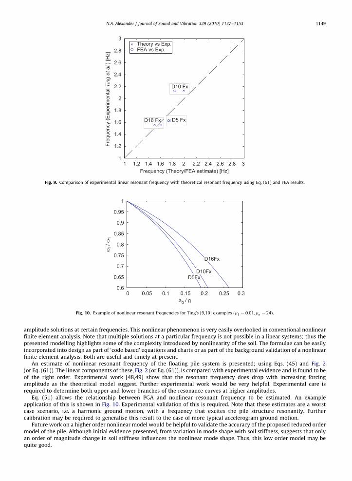
Fig. 9. Comparison of experimental linear resonant frequency with theoretical resonant frequency using Eq. (61) and FEA results.

0 0.05 0.1 0.15 0.2 0.25 0.30.6

0.65

0.7

0.75

0.8

0.85

0.9

0.95

1

D5FxD10Fx

D16Fx

ag / g

ωr /

ω1

Fig. 10. Example of nonlinear resonant frequencies for Ting’s [9,10] examples ðm1 ¼ 0:01;mn ¼ 24Þ.


amplitude solutions at certain frequencies. This nonlinear phenomenon is very easily overlooked in conventional nonlinearfinite element analysis. Note that multiple solutions at a particular frequency is not possible in a linear systems; thus thepresented modelling highlights some of the complexity introduced by nonlinearity of the soil. The formulae can be easilyincorporated into design as part of ‘code based’ equations and charts or as part of the background validation of a nonlinearfinite element analysis. Both are useful and timely at present.

An estimate of nonlinear resonant frequency of the floating pile system is presented; using Eqs. (45) and Fig. 2(or Eq. (61)). The linear components of these, Fig. 2 (or Eq. (61)), is compared with experimental evidence and is found to beof the right order. Experimental work [48,49] show that the resonant frequency does drop with increasing forcingamplitude as the theoretical model suggest. Further experimental work would be very helpful. Experimental care isrequired to determine both upper and lower branches of the resonance curves at higher amplitudes.

Eq. (51) allows the relationship between PGA and nonlinear resonant frequency to be estimated. An exampleapplication of this is shown in Fig. 10. Experimental validation of this is required. Note that these estimates are a worstcase scenario, i.e. a harmonic ground motion, with a frequency that excites the pile structure resonantly. Furthercalibration may be required to generalise this result to the case of more typical accelerogram ground motion.

Future work on a higher order nonlinear model would be helpful to validate the accuracy of the proposed reduced ordermodel of the pile. Although initial evidence presented, from variation in mode shape with soil stiffness, suggests that onlyan order of magnitude change in soil stiffness influences the nonlinear mode shape. Thus, this low order model may bequite good.

ARTICLE IN PRESS


The introduction of varying width of near-field soil layer would allow the model to have a variation in effective soilmass with depth. It is likely that more soil motion occurs near the pile head and thus more mass should be included here. Itis highly desirable to perform careful experimental studies to ascertain the volume of soil that should be included in thenear-field.

Acknowledgement

The author acknowledges the support of the University of Bristol. Deo Gratias.

Appendix A. Example of obtaining set of orthogonal polynomials that satisfy the boundary conditions

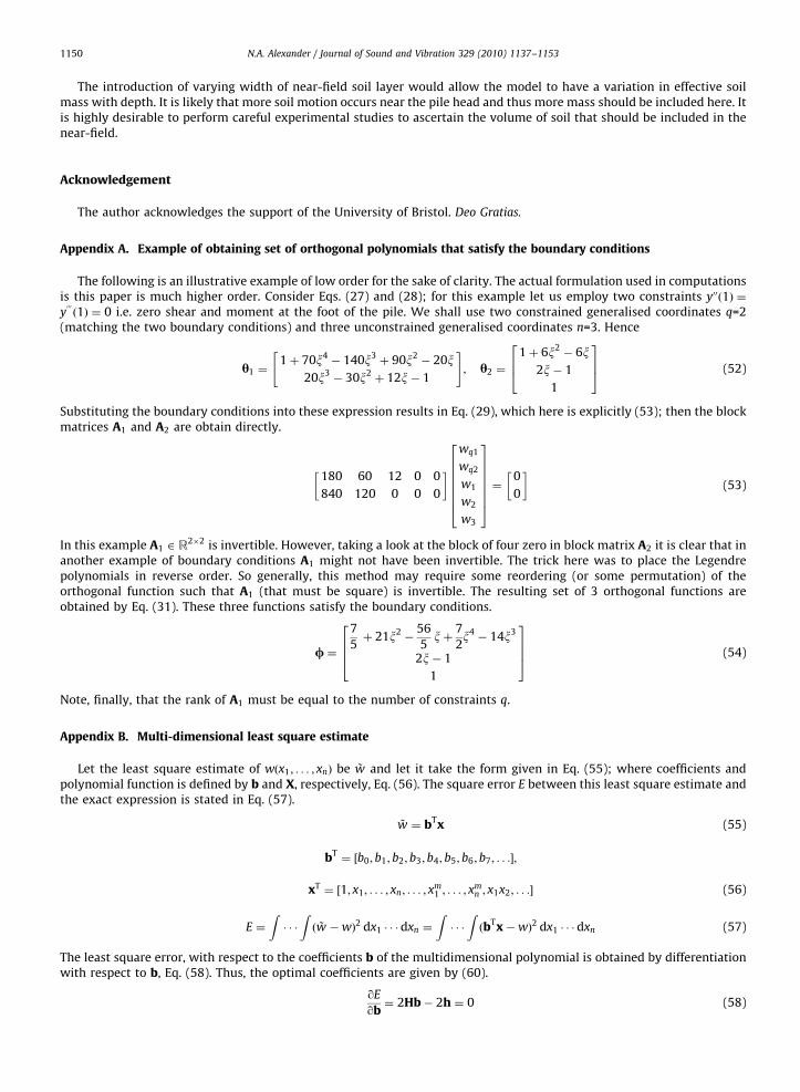
The following is an illustrative example of low order for the sake of clarity. The actual formulation used in computationsis this paper is much higher order. Consider Eqs. (27) and (28); for this example let us employ two constraints y00ð1Þ ¼y000

ð1Þ ¼ 0 i.e. zero shear and moment at the foot of the pile. We shall use two constrained generalised coordinates q=2(matching the two boundary conditions) and three unconstrained generalised coordinates n=3. Hence

h1 ¼1þ 70x4

� 140x3þ 90x2

� 20x20x3

� 30x2þ 12x� 1

" #; h2 ¼

1þ 6x2� 6x

2x� 1

1

264

375 (52)

Substituting the boundary conditions into these expression results in Eq. (29), which here is explicitly (53); then the blockmatrices A1 and A2 are obtain directly.

180 60 12 0 0

840 120 0 0 0

� �wq1

wq2

w1

w2

w3

26666664

37777775¼

0

0

� �(53)

In this example A1 2 R2�2 is invertible. However, taking a look at the block of four zero in block matrix A2 it is clear that in

another example of boundary conditions A1 might not have been invertible. The trick here was to place the Legendrepolynomials in reverse order. So generally, this method may require some reordering (or some permutation) of theorthogonal function such that A1 (that must be square) is invertible. The resulting set of 3 orthogonal functions areobtained by Eq. (31). These three functions satisfy the boundary conditions.

/ ¼

7

5þ 21x2

�56

5xþ

7

2x4� 14x3

2x� 1

1

2664

3775 (54)

Note, finally, that the rank of A1 must be equal to the number of constraints q.

Appendix B. Multi-dimensional least square estimate

Let the least square estimate of wðx1; . . . ; xnÞ be ~w and let it take the form given in Eq. (55); where coefficients andpolynomial function is defined by b and X, respectively, Eq. (56). The square error E between this least square estimate andthe exact expression is stated in Eq. (57).

~w ¼ bTx (55)

bT¼ ½b0;b1; b2; b3;b4; b5; b6; b7; . . .�;

xT ¼ ½1; x1; . . . ; xn; . . . ; xm1 ; . . . ; x

mn ; x1x2; . . .� (56)

E ¼

Z� � �

Zð ~w �wÞ2 dx1 � � �dxn ¼

Z� � �

ZðbTx�wÞ2 dx1 � � �dxn (57)

The least square error, with respect to the coefficients b of the multidimensional polynomial is obtained by differentiationwith respect to b, Eq. (58). Thus, the optimal coefficients are given by (60).

qE

qb¼ 2Hb� 2h ¼ 0 (58)

ARTICLE IN PRESS


H ¼Z� � �

ZxxT dx1 � � �dxn; h ¼

Z� � �

Zxw dx1 � � � dxn (59)

b ¼ H�1h (60)

Appendix C. Approximate formula for linear natural frequency x1

In this paper, the actual linear mode has been adopted for spatial shape function of the pile, fðxÞ. This linearfundamental mode is obtained from a high order linear eigenvalue problem, see Section 3.1. In obtaining this eigenvector,the eigenvalue is also obtained and hence o1, see Fig. 2. However, for more than 4 generalised coordinates, it is notpossible to obtain a closed form expression for this eigenvalue (root); Abel–Ruffini theorem. Thus, no simple and accurateclosed form expression for o1 is obtainable using this approach.

In addition, a least square expression for o1ða;Z1Þ was sought. However, no really good fit was easily achievable. So, asan alternate, an approximation of this linear mode shape was sought. It was obtained by applying a horizontal force at thepile head and using the pile deflected shape as an approximation to the linear mode. This approach only requires theinversion of the stiffness matrix K that is analytically obtainable in closed form for higher order systems. This was thenused to obtain an closed form expression for o1ða;Z1Þ using Eqs. (10) and (14); resulting in Eq. (61).

o1Cs

ffiffiffiffiffisn

sd

r(61)

Formulae for sn and sd are given in Appendices C, D and E. Note that formula (61) is a very good engineering approxi-mation. The correlation between (61) and Fig. 2 is high ðR2 ¼ 0:99Þ. Thus, it can be concluded, for this problem, thatapplication of a point load at the lumped head mass produces an accurate estimate of the first mode across the entire spaceða;Z1Þ likely to be encountered in practice.

Appendix D. Floating toe pile without cap formulae

f ¼qn

qd(62)

qn ¼ ð1:855E7Z1 � 2:172E4Z21Þx

6� ð4:174E7Z1 � 8:26E4Z2

1Þx5� � �

�1:125E5x4Z21 þ ð4:638E7Z1 þ 5:815E4Z2

1Þx3� � �

�ð6:68E9þ 3:403E7Z1 þ 8220Z21Þxþ ð5:01E9þ 1:18E7Z1 þ 1547Z2

1Þ (63)

qd ¼ 1547Z21 þ 1:18E7Z1 þ 5:009E9 (64)

The functions, sn and sd, required to determine the linear frequency parameter o1in equation (61) are given by (65) and(66), respectively.

sn ¼ Z1ð1:534E11Z41 þ 5:273E15Z3

1 þ 3:783E19Z21 þ 1:951E25þ 5:926E22Z1Þ (65)

sd ¼ ð3:35E13Z41 þ 5:112E17Z3

1 þ 2:167E21Z21 þ 1:655E24Z1 þ 3:512E26Þa � � �

þ2:335E12Z41 þ 4:233E16Z3

1 þ 2:629E20Z21 þ 2:556E23Z1 þ 9:106E25 (66)

Appendix E. Floating toe pile with cap formulae

f ¼qn

qd(67)

qn ¼ ð9:419E6Z21 � 5822Z3

1Þx6� ð2:186E8Z1 þ 2:38E7Z2

1 � 2:361E4Z31Þx

5� � �

þð4:964E6Z21 � 3:619E4Z3

1Þx4� � � þ ð2:186E9Z1 þ 2:97E7Z2

1 þ 2:505E4Z31Þx

3� ð4:372E9Z1

þ2:222E7Z21 þ 6856Z3

1Þx2� � � þ ð2:624E10þ 1:748E9Z1 þ 2:172E6Z2

1 þ 181Z31Þ (68)

qd ¼ 181Z31 þ 2:173E6Z2

1 þ 1:747E9Z1 þ 2:624E10 (69)

ARTICLE IN PRESS


The functions, sn and sd, required to determine the linear frequency parameter o1 in Eq. (61) are given by (70) and (71)respectively.

sn ¼ Z1ð1:534E11Z41 þ 5:273E15Z3

1 þ 3:783E19Z21 þ 1:951E25þ 5:926E22Z1Þ (70)

sd ¼ ð3:35E13Z41 þ 5:112E17Z3

1 þ 2:167E21Z21 þ 1:655E24Z1 þ 3:512E26Þa � � �

þ2:335E12Z41 þ 4:233E16Z3

1 þ 2:629E20Z21 þ 2:556E23Z1 þ 9:106E25 (71)

References

[1] S. Bhattacharya, S. Adhikari, N.A. Alexander, A simplified method for unified buckling and dynamic analysis of pile supported structures inseismically liquefiable soils, Soil Dynamics and Earthquake Engineering 29 (2009) 1220–1235.

[2] R.L. Kondner, Hyperbolic stress–strain response: cohesive soils, Journal of the Soil Mechanics and Foundations Division 89 (1963) 115–144.[3] Det Norske Veritas, Rules for the design, construction, and inspection of offshore structures, Appendix F; Foundations, Hovik, Norway, 1980.[4] R.F. Scott, Analysis of Centrifuge Pile Tests; Simulation of Pile Driving, American Petroleum Institute, Washington, DC, USA, 1980.[5] H. Matlock, Correlations for design of laterally loaded piles in soft clay, Proceedings of the Second Annual Offshore Technology Conference, Houston, USA,

1970.[6] L.C. Reese, W.R. Cox, F.D. Koop, Analysis of laterally loaded piles in sand, Proceedings of the Sixth Annual Offshore Technology Conference, Houston, USA,

1974.[7] J.M. Murchison, M.W. O’Neill, Evaluation ofP–Y Relationships in Cohesionless Soils, San Francisco, CA, USA, 1984, pp. 174–191.[8] W. Finn, A study of piles during earthquakes: issues of design and analysis, Bulletin of Earthquake Engineering (2005) 141–234.[9] J.M. Ting, C.R. Kauffman, M. Lovicsek, Centrifuge static and dynamic lateral pile behaviour, Canadian Geotechnical Journal 24 (1987) 198–207.

[10] J.M. Ting, Full-scale cyclic dynamic lateral pile responses, Journal of Geotechnical Engineering 113 (1987) 30–45.[11] M.H. El Naggar, K.J. Bentley, Dynamic analysis for laterally loaded piles and dynamic p–y curves, Canadian Geotechnical Journal 37 (2000) 1166–1183.[12] API, Recommended Practice for Planning, Designing and Constructing Fixed Offshore Platforms—Working Stress Design—Includes Supplement 2, American

Petroleum Institute, 2000.[13] J. Brinch Hansen, The Ultimate Resistance of Rigid Piles Against Transversal Forces, Danish Geotechnical Institute, Copenhagen, Denmark, Vol. 12,

1961, pp. 5–9.[14] W.G.K. Fleming, A.J. Weltman, M.F. Randolph, W.K. Elson, Piling Engineering, Surrey University Press, London, 1992.[15] L. Zhang, F. Silva, R. Grismala, Ultimate lateral resistance to piles in cohesionless soils, Journal of Geotechnical and Geoenvironmental Engineering 131

(2005) 78–83.[16] M. Randolph, The challenges of offshore geotechnical engineering, Ground Engineering 38 (2005) 32–33.[17] B.T. Kim, N.-K. Kim, W.J. Lee, Y.S. Kim, Experimental load-transfer curves of laterally loaded piles in Nak-Dong River sand, Journal of Geotechnical and

Geoenvironmental Engineering 130 (2004) 416–425.[18] Dynamic Analysis and Earthquake Resistant Design, Strong Motion and Dynamic Properties, vol. 1, Japanese Society of Civil Engineers, A.A. Balkema,

Rotterdam, Brookfield, 1997.[19] L. Verdure, J. Garnier, D. Levacher, Lateral cyclic loading of single piles in sand, International Journal of Physical Modelling in Geotechnics 3 (2003)

17–28.[20] P.J. Holmes, D.A. Rand, Bifurcations of Duffings equation—application of catastrophe theory, Journal of Sound and Vibration 44 (1976) 237–253.[21] Y. Ueda, Randomly transitional phenomena in the system governed by Duffings equation, Journal of Statistical Physics 20 (1979) 181–196.[22] C. Pezeshki, E.H. Dowell, On chaos and fractal behavior in a generalized Duffings system, Physica D 32 (1988) 194–209.[23] F.N.H. Robinson, Experimental-observation of the large-amplitude solutions of Duffings and related equations, IMA Journal of Applied Mathematics 42

(1989) 177–201.[24] L.C. Reese, H. Matlock, Non-dimensional solutions for laterally loaded piles with soil modulus assumed proportional tp depth, Proceedings of the

Eighth Texas Conference on Soil Mechanics and Foundation Engineering, Austin, TX, 1956, pp. 1–41.[25] G. Rega, A.H. Nayfeh, Nonlinear Interactions: Analytical, Computational, and Experimental Methods, Wiley Series in Nonlinear Science, Vol. 760, Wiley,

New York, 2000 (Meccanica, 35 (2000) 583–586).[26] E. Gourdon, N.A. Alexander, C.A. Taylor, C.H. Lamarque, S. Pernot, Nonlinear energy pumping under transient forcing with strongly nonlinear

coupling: theoretical and experimental results, Journal of Sound and Vibration 300 (2007) 522–551.[27] E.J. Doedel, A.R. Champneys, T.F. Fairgrieve, Y.A. Kuznetsov, B. Sandstede, X. Wang, AUTO 97: Continuation and Bifurcation Software for Ordinary

Differential Equations (with HomCont), Technical Report, Concordia University, 1997.[28] N.A. Alexander, F. Schilder, Exploring the performance of a nonlinear tuned mass damper, Journal of Sound and Vibration 319 (2009) 445–462.[29] A.H. Nayfeh, N.E. Sanchez, Bifurcations in a forced softening Duffing oscillator, International Journal of Non-Linear Mechanics 24 (1989) 483–497.[30] L.N. Virgin, L.A. Cartee, A note on the escape from a potential well, International Journal of Non-Linear Mechanics 26 (1991) 449–452.[31] K. Yagasaki, Detection of bifurcation structures by higher-order averaging for Duffing’s equation, Nonlinear Dynamics 18 (1999) 129–158.[32] C. Hayashi, Non-linear Oscillations in Physical Systems, McGraw-Hill, New York, 1964.[33] MATLAB (the language of technical computing), seventh ed., The Mathworks Inc., 2005.[34] T. Koskusho, Dynamic Deformation Properties of Soil and Nonlinear Seismic Response, Vol. 301, Central Research Institute of Electric Power Industry,

Japan, 1982.[35] K. Nishi, Y. Yoshida, Y. Sawada, T. Iwadate, T. Kokusyo, Soil-structure interaction of JPDR reactor, 2. Static and dynamic mechanical properties of sand

and sandy gravel by laboratory tests and proposal of model of ground, Denryoku Chuo Kenkyusho Hokoku (Japan) 383002 (1983) 1–44.[36] B.O. Hardin, V.P. Drnevich, Shear modulus and damping in soils: measurement and parameter effects, American Society of Civil Engineers, Journal of

the Soil Mechanics and Foundations Division 98 (1972) 603–624.[37] M.L. Silver, H.B. Seed, Deformation characteristics of sands under cyclic loading, Journal of the Soil Mechanics and Foundations Division 97 (1971)

1081–1098.[38] N.A. Alexander, Evaluating basins of attraction in non-linear dynamical systems using an improved recursive boundary enhancement (RBE), Journal

of Sound and Vibration 209 (1998) 443–447.[39] N.A. Alexander, Evaluating the global characteristic of a nonlinear dynamical system with recursive boundary enhancement, Advances in Engineering

Software 29 (1998) 707–716.[40] J.M.T. Thompson, S.R. Bishop, L.M. Leung, Fractal basins and chaotic bifurcations prior to escape from a potential well, Physics Letters A 121 (1987)

116–120.[41] F.E. Richart, J.R. Hall, R.D. Woods, Vibrations of Soils and Foundations, Prentice-Hall, Inc., 1970.[42] S. Adhikari, S. Bhattacharya, Dynamic instability of pile-supported structures in liquefiable soils during earthquakes, Journal of Shock and Vibration,

2008.[43] S. Bhattacharya, A. Blackborough, S.R. Dash, Collapse of piled-foundations in liquefiable soils-an example of design-based error, Proceedings of the

Institution of Civil Engineers, Civil Engineering, UK, 2008.

ARTICLE IN PRESS


[44] S. Bhattacharya, S.R. Dash, S. Adhikari, On the mechanics of failure of pile-supported structures in liquefiable deposits during earthquakes, CurrentScience 94 (2008) 605–611.

[45] S. Bhattacharya, S.P.G. Madabhushi, M.D. Bolton, An alternative mechanism of pile failure in liquefiable deposits during earthquakes, Geotechnique54 (2004) 203–213.

[46] K.M. Rollins, K.T. Peterson, T.J. Weaver, Lateral load behavior of full-scale pile group in clay, Journal of Geotechnical and Geoenvironmental Engineering124 (1998) 468–478.

[47] K.M. Rollins, J.D. Lane, T.M. Gerber, Measured and computed lateral response of a pile group in sand, Journal of Geotechnical and GeoenvironmentalEngineering 131 (2005) 103–114.

[48] J.F. Stanton, S. Banerjee, I. Hasayen, Shaking table tests on piles, University of Washington, USA, 1988.[49] A. Boominathan, R. Ayothiraman, Dynamic behaviour of laterally loaded model piles in clay, Proceedings of the Institution of Civil Engineers:

Geotechnical Engineering 158 (2005) 207–215.

estimating the nonlinear resonant frequency of a single

Documents