IOP PUBLISHING JOURNAL OF GEOPHYSICS AND ENGINEERING

J. Geophys. Eng. 5 (2008) 54–66 doi:10.1088/1742-2132/5/1/006

Nonlinear inversion for estimatingreservoir parameters from time-lapseseismic dataMohsen Dadashpour, Martin Landrø and Jon Kleppe

Department of Petroleum Engineering and Applied Geophysics, NTNU, 7491, Trondheim, Norway

E-mail: dadashpo@stud.ntnu.no, martin.landro@ntnu.no and jon.kleppe@ntnu.no

Received 3 October 2006Accepted for publication 18 September 2007Published 28 November 2007Online at stacks.iop.org/JGE/5/54

AbstractSaturation and pore pressure changes within a reservoir can be estimated by a history matchingprocess based on production data. If time-lapse seismic data are available, the sameparameters might be estimated directly from the seismic data as well. There are several waysto combine these data sources for estimating these reservoir parameters. In this work, weformulate a nonlinear inversion scheme to estimate pressure and saturation changes fromtime-lapse seismic data. We believe that such a formulation will enable us to include seismicdata in the reservoir simulator in an efficient way, by including a second term in the least-squares objective function. A nonlinear Gauss–Newton inversion method is tested on a 2Dsynthetic dataset inspired by a field offshore from Norway. A conventional reservoir simulatorhas been used to produce saturation and pore pressure changes as a function of productiontime. A rock physics model converts these data into synthetic time-lapse seismic data. Finally,the synthetic time-lapse data are used to test the derived inversion algorithm. We find that theinversion results are strongly dependent on the input model, and this is expected since we aredealing with an ill-posed inversion problem. Since we estimate pressure and saturation changefor each grid cell in the reservoir model, the number of model parameters is high, andtherefore the problem is undetermined. From testing, using this particular dataset, we assumeneither pressure nor saturation changes for the initial model. Although uncertainties associatedwith the proposed method are high, we think this might be a useful tool, since there are waysto reduce the number of model parameters and constrain the objective function by includingproduction data and reservoir simulation data into this algorithm.

Keywords: saturation and pressure changes, time-lapse seismic, parameter estimation,inversion, reservoir simulation

Nomenclature

H Hessian matrixc average number of contacts per graind production quantitiesF objective functionf data residual vectorError normalized errorJ Jacobian matrixkeff effective bulk moduluskfr bulk modulus of solid framework

kg gas bulk moduluskL bulk modulus of the liquidskma bulk modulus for solidko oil bulk moduluskw water bulk modulusMERR minimum errorMAXIT maximum iteration numberN number of parametersNRMS normalized RMSP reservoir pore pressurePbub bubble point pressure

1742-2132/08/010054+13$30.00 © 2008 Nanjing Institute of Geophysical Prospecting Printed in the UK 54

Nonlinear inversion for estimating reservoir parameters from time-lapse seismic data

Peff effective pressurePext external pressureRMS root mean squareSg gas saturationSo oil saturationSor residual oil saturationSw water saturationSwc irreducible water saturationVp P-wave velocityVs S-wave velocityV Poisson ratioµeff effective shear modulusα model parameter vectorδα error vector�α amount of perturbation of the function.M shear modulus of solid frameworkρ bulk densitiesρ f fluid densitiesρma matrix densitiesϕ porosity

Subscripts and superscripts

nobs number of observationnpar number of parameterobs observedcal calculatednc number of cellsi data space (indicator from 1 to npar)j model space (indicator from 1 to nobs)ˆ scaled (Hessian, gradient, . . . )

1. Introduction

An ultimate goal in reservoir engineering is to build a modelthat is as close as possible to nature. This model should beable to predict all crucial data acquired during field production,and at the same time access predictive features suitable forreservoir management. History matching is the method usedto meet this goal. History matching involves a construction ofan initial model with an initial approximation of the reservoirparameters, followed by a systematic process to minimizean objective function that represents the mismatch betweenobserved and simulated responses. This optimization processis for instance achieved by perturbing the relevant parameters,and determining updates that reduce the objective function.Parameter estimation or determination of reservoir propertiesis one useful application of the history matching process,which is a well-established method for reservoir propertyestimation.

Reservoir fluid saturation and pore pressure changeshave direct relationships with the drainage and recoveryof the reservoir. Robust estimation of changes in theseparameters during the life of a hydrocarbon field will leadto well founded future predictions and decisions in reservoirmanagement, and thus will increase the ultimate recovery fromthe reservoir and reduce the production costs. Furthermore,increased knowledge about these crucial reservoir parameters

will ensure safer and more environmental friendly productionof hydrocarbons.

There are many methods for estimation of theseparameters. Traditionally, reservoir fluid flow simulators areused for this purpose. These methods estimate reservoirparameters primarily based on traditionally known observationdata such as bottom hole pressure (Slater and Durrer 1971,Thomas et al 1971), oil, water and gas production data (Tan1995), well test shut-in pressure data (Landa et al 1996) andsome combinations of these data (Schulze-Riegert et al 2001,Aanonsen et al 2003). However, traditional history matchingis associated with several uncertainties such as the following.

• Parameters from individual wells are not representing allreservoir compartments and zones (up-scaling problem).

• Fluid flow formulae are associated with someuncertainties.

• The geological description of the reservoir model isalways a simplification of nature, and we must thereforeexpect that some production related effects cannot be fullyexplained by the idealized reservoir model.

• In most cases, consideration of all production processesin reservoir simulation is both numerically expensive andextremely difficult to simulate correctly.

Because of these uncertainties in the fluid flow simulators,there might be a significant difference between historical andnumerically modelled data. Calibration or conditioning ofthe reservoir simulation models to fit the historical productiondata is history matching. Usually, history matching requiresnumerous iterations that are time consuming and costly, and itis also a non-unique problem.

Domenico (1974) and Nur (1989) investigated the effectof saturation and pressure changes on seismic parameters.They have concluded that changing these parameters has adetectable effect in seismic attributes. Landrø (2001) triedto map the reservoir pressure and saturation changes usingseismic methods. Landrø (2001) tried to represent an efficientmethod to discriminate between pressure and saturation effectsfrom time-lapse seismic data. Recently, time-lapse, or 4D,seismic data have become available as an additional set ofdynamic data. Time-lapse seismic is now a useful tool formonitoring thermal processes (Eastwood et al 1994), CO2

flooding (Lazaratos and Marion 1997) as well as gas and waterinjection (Landrø et al 1999, Burkhart et al 2000, Behrenset al 2002).

Today, 4D seismic data are used to monitor fluidmovements within the reservoir. This is a new dimensionfor history matching since 4D seismic contains informationabout fluid movement and pressure changes between andbeyond the wells. Most reservoir parameters which are beingused in reservoir simulators are estimated from laboratorymeasurements that are not representative of the entire reservoir.By integrating time-lapse data with the production data ina history matching process, the uniqueness of the resultsimproves. Many authors try to update the model by usingthis additional information (Landa and Horne 1997, VanDitzhuijzen et al 2001, Mantica et al 2001, Kretz et al2004). They ignored the first step of inversion that means they

55

M Dadashpour et al

assumed time-lapse seismic is already converted to saturationchanges and in addition they assumed seismic variations wereonly a result of saturation changes and they ignored pressureeffects. This research addresses this missing part.

Estimation of saturation and pressure changes using time-lapse seismic data is a new challenge in the petroleum industry.This is the first step in history matching using both reservoirsimulation and time-lapse seismic data. In this paper wepresent a nonlinear inversion method for a joint estimationof pressure and saturation changes during depletion and waterinjection of a 2D synthetic case, which is generated by usingfield data from a reservoir offshore from Norway.

2. Forward seismic modelling

Key reservoir parameters, such as saturations and pressures,are changing during production and this might causesignificant changes in the seismic responses. Highly poroussand reservoirs show significant 4D seismic changes, whilelow porosity carbonate reservoirs show less 4D changes.Time-lapse seismic data are time-dependent measurements(dynamic measurements), acquired from the reservoir usingthe same acquisition parameters for the various time-lapseseismic surveys. Converting saturations and pressure changesinto seismic properties such as P-wave velocity, S-wavevelocity and density changes requires information about therock properties. The dependence between fluid saturationchanges and pore pressure changes and the seismic parametersare described by rock physics models. Once these rockphysics relationships are established for a given reservoirrock, the seismic forward modelling can be done. Thatmeans converting a given pressure and fluid saturation statefor a given reservoir rock into a seismic section. Moreover,this procedure acts as a bridge that relates seismic parameterchanges to reservoir parameter changes and vice versa. Thus,understanding this part of the inversion loop is vital for doinggood history matching. This means that rock physics is a keyelement in such a process. Uncertainties and systematic errorsin the rock physics model will be of crucial importance to thefinal result. The main limitation of the calibrated rock physicsmodels is that they cannot capture variations in rock propertiesbetween wells.

Seismic amplitudes change with variation in the sourcestrength and with the angle of incidence. In addition, variationsin acoustic properties are the function of reservoir propertiessuch as pressure, fluid saturation, temperature and compaction.Effects of temperature and compaction are not considered inthis work.

Forward modelling is done in two main steps. First,reservoir parameters are converted to seismic parameters byusing the rock physics models. The Gassmann equation(Gassmann 1951) and the Hertz–Mindlin model (Mindlin1949) are used to estimate seismic parameter changes causedby fluid saturation and pore pressure changes, respectively.Then, synthetic seismic sections are calculated based on theseparameters. For simplicity, a one-dimensional reflectivity-based modelling is used. This scheme includes internalmultiple reflections. In this case, the reflection coefficients

are defined by contrasts in acoustic impedance. The two-waytravel time is computed from the P-wave velocity. Time-lapsechanges in reflection strength are caused by changes in acousticimpedance. 4D time shifts are introduced by changes in P-wave velocity within the reservoir layers. Both impedanceand velocity are saturation–pressure dependent (Stovas andLandrø 2005).

We study a two-phase system (oil and water) and focuson variation of oil and water saturation, denoted by So and Sw,respectively.

2.1. The Gassmann equation

Seismic velocities in a porous medium saturated with waterdepend on three constants, namely the bulk modulus k (weuse the lowercase letter to avoid any confusion with thepermeability sign), shear modulus µ and density ρ. The bulkmodulus or incompressibility of an isotropic rock is definedas the ratio of hydrostatic stress to volumetric strain. In otherwords, it tells us how difficult it is to compress the rock. Theshear modulus or shear stiffness of the rock is defined as theratio of shear stress to shear strain and in other words, howdifficult it is to change the shape of a rock sample. In the long-wavelength limit, the speed of sound is related to the elasticconstants of the aggregate:

vp =√

k + 43µ

ρB

, (1)

vs =√

µ

ρB

, (2)

where ρB denotes bulk density, i.e. the volume average densityof the solid and liquid phases, which is a function of porosity,matrix and fluid densities and can be calculated from thefollowing equation:

ρB = φρf + (1 − φ)ρma, (3)

where ρ f and ρma are the fluid and matrix densities,respectively. The downscaling steps allow the calculation ofthe fluid density:

ρf = ρoSo + ρwSw, (4)

where ρo and ρw are oil and water densities, respectively.The most commonly used theoretical approach for fluidsubstitution employs the low-frequency Gassmann theory.The Gassmann equations divide the bulk modulus of a fluidsaturated rock into three parts:

• the bulk modulus of the mineral matrix,• the bulk modulus of the porous rock frame,• the bulk modulus of the pore-filling fluids.

Gassmann equations can be written as the followingformula:

ksat = kf r +(kHM − kf r)

2

kHM(1 − φ + φ kHM

kf− kf r

kHM

) , (5)

where kfr is the bulk modulus of the solid framework,kHM is the bulk modulus of the Hertz–Mindlin formula

56

Nonlinear inversion for estimating reservoir parameters from time-lapse seismic data

(equation (7)), kf is the bulk modulus of the saturating fluid(water, gas or oil) and φ is the effective porosity of the medium.kf is the bulk modulus of the pore fluid (water and oil) and isestimated by Wood’s law for oil and water given as (Reussharmonic average 1929):

1

kf

= So

ko

+Sw

kw

, (6)

where ko and kw denote oil and water bulk modulus,respectively.

According to Mavko et al (1998) the Gassmann equationis associated with some assumptions:

• Pore fluid is firmly coupled to the pore wall.• Gas and liquid are uniformly distributed in the pores.• Constant shear modulus in dry and saturated rocks.• There is homogeneous mineral modulus and statistical

isotropy.

However, there is no assumption made about the poregeometry. In addition, the Gassmann equation is only validfor low frequencies when the pore pressures are equilibratedthrough the pore space.

2.2. The Hertz–Mindlin model

The Hertz–Mindlin model is used to describe seismicparameter changes caused by pressure changes. The effectivebulk modulus and shear modulus of a dry random identicalsphere packing are given by

kHM = n

√c2(1 − φc)2µ2peff

18π2(1 − ν)2, (7)

µHM = 5 − 4ν

5(2 − ν)

n

√3c2(1 − φc)2µ2peff

2π2(1 − ν)2, (8)

where kHM and µHM are the bulk and shear modulus at criticalporosity φc, respectively; Peff is the effective pressure; µ is theshear modulus of the solid phase; ν is Poisson’s ratio and n isthe coordination number. In the original Hertz–Mindlin theoryn is equal to 3 which means velocity varies with Peff raised tothe 1/6th power. Some laboratory measurements of samplesgave a larger number for n. Vidal (2000) found n = 5.6 forP-waves and n = 3.8 for S-waves for gas sands, while Landrø(2001) used n = 5 for oil sands. We have used n = 5 in thiswork. c denotes the average number of contacts per grain, andin this study we use c = 9. The effective pressure, Peff, usedin Hertz–Mindlin theory is taken as the difference between thelithostatic Pext and the hydrostatic pressure P (Christensen andWang 1985):

Peff = Pext − ηP, (9)

where η is the coefficient of internal deformation whichis usually an unknown parameter. Thus, it is a limitingfactor for quantitative use of rock physics measurements forpore pressure estimation. This unknown parameter is oftenassumed to be equal to 1; however, if η is different from 1,uncertainty in estimation in saturation and pressure changeswill increase.

3. Inversion method

The inversion model or parameter estimation proceduredetermines the values of reservoir parameters such as pressureand saturation from indirect measurements. This proceduretraditionally starts with an initial guess of body parametersand the process is iteratively advanced until the best fit isobtained between the calculated and observed data. Thecommon algorithm for an inversion process is as follows:

(1) Enter the initial guess for the body parameters.(2) Compute the response of the system through forward

modelling.(3) Compute the objective function.(4) Update parameters by minimizing the objective function

using some minimization algorithms.(5) If the value of the objective function is not certifiable,

return to step 2.

Several optimization algorithms are developed for thispurpose. Some of these, such as Gauss–Newton, singularvalue decomposition, conjugate gradient and steepest descent(Landa 1979, Gill et al 1981) require both or at least one ofthe first (Jacobian) or second (Hessian) derivative of time-dependent reservoir properties with respect to static reservoirproperties. However, some of them such as genetic algorithm,response surfaces, experimental design methods and MonteCarlo simulation (Lepine et al 1998) do not require thecomputation of gradients for optimization purpose.

In this work, minimization of the objective function issolved numerically by the damped Gauss–Newton method(appendix A) which is classified as a gradient-based methodto determine the target parameters automatically. The mainpurpose of each inversion method is to minimize an objectivefunction, which is defined as deviation between the calculatedvalue (dcal) and the observed value (dobs). In this study d isamplitude differences between the base and monitor survey(time-lapse seismic data):

F =N∑

i=1(f )2

f = (dobs − dcal),

(10)

where N is the number of observation points, f is the dataresidual vector and F is the least-squares error, which shouldbe minimized.

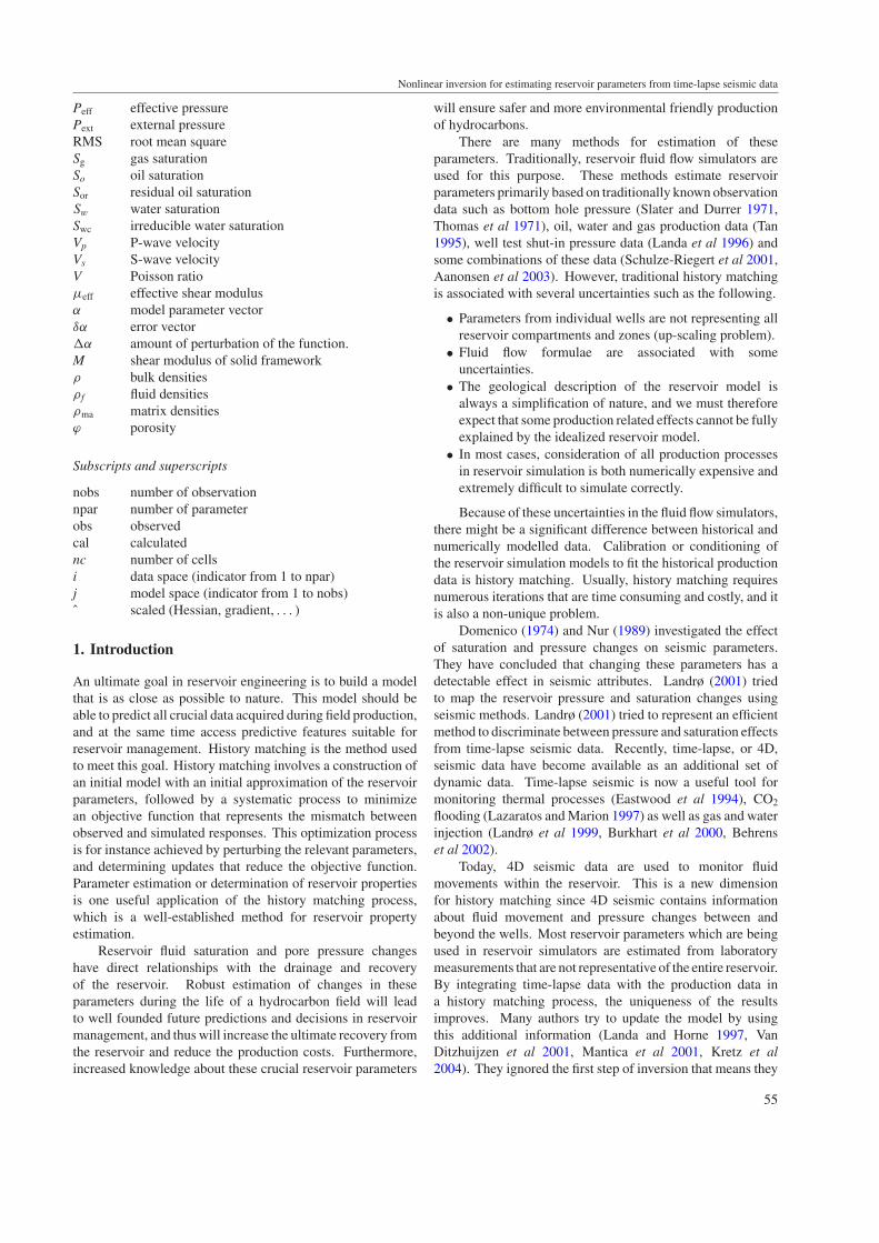
The inversion procedure is summarized in figure 1 andconsists of the following steps.

(1) Enter initial guess of parameters (αi), observationdata

(dobs

j

), maximum iteration number (MITR) and

minimum acceptable error (MERR). Inverted parametersare saturation and pressure changes for each cell and aredefined as

αi = [�S1 . . . �Snc,�P1 . . . �Pnc] ,(11)

nc = number of cells.

57

M Dadashpour et al

Figure 1. Flowchart of the nonlinear inversion process.

(2) Compute the calculated data(dcal

j

)by using forward

seismic modelling.

(3) Calculate the Jacobian matrix which is defined as Jij =∂di/∂αi where i runs over data space, j runs over modelspace and α is the model parameter vector (appendix A.2).

(4) Calculate the transpose of the Jacobian matrix (JT).

(5) Calculate the objective function (F) from equation (10).

(6) If the error is less than the minimum acceptable error or theiteration numbers are higher than the maximum iterationnumber, stop and print the iteration number and the newvalues for the parameters.

(7) Compute the gradient matrices (G), G = −2J T f , andcompute the approximate Hessian matrix (H) H = 2J T J .Based on Helgesen and Landrø (1993) each parameterclass is scaled independently in order to speed up thealgorithm. The scaling formulae are

�

H ij = Hij√HjjHii

�

Gii = Gii√Hii

. (12)

(8) Calculate the normalized Hessian and gradient matrices.

(9) Calculate the scaled model parameter:

H .δp = −G δαi = δαi√Hii

. (13)

(10) Update the parameter by adding the update vector to theold value:

αi = αi + δαi, (14)

(11) Apply constraints for these values to have reasonablevalue.

(12) Add one value to the iteration number.

(13) Go to step 2.

4. Example

To test the efficiency and accuracy of our method, we designeda 2D synthetic experiment based on a 2D cross section froma North Sea reservoir model. The propagator-matrix method(Haskell 1953, Kennett 1983) which is modified by Stovas andArntsen (2006) for a quasi-vertical wave propagation approachwas used to compute the transmission and reflection responsefrom a stack of plane layers. Based on the modelled time-lapse seismic differences, changes in fluid saturations and porepressure for each cell in the reservoir model were estimated.

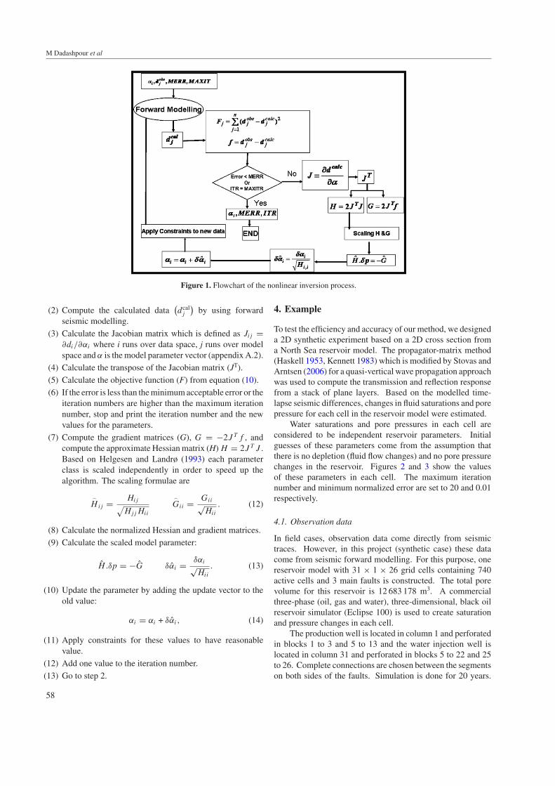
Water saturations and pore pressures in each cell areconsidered to be independent reservoir parameters. Initialguesses of these parameters come from the assumption thatthere is no depletion (fluid flow changes) and no pore pressurechanges in the reservoir. Figures 2 and 3 show the valuesof these parameters in each cell. The maximum iterationnumber and minimum normalized error are set to 20 and 0.01respectively.

4.1. Observation data

In field cases, observation data come directly from seismictraces. However, in this project (synthetic case) these datacome from seismic forward modelling. For this purpose, onereservoir model with 31 × 1 × 26 grid cells containing 740active cells and 3 main faults is constructed. The total porevolume for this reservoir is 12 683 178 m3. A commercialthree-phase (oil, gas and water), three-dimensional, black oilreservoir simulator (Eclipse 100) is used to create saturationand pressure changes in each cell.

The production well is located in column 1 and perforatedin blocks 1 to 3 and 5 to 13 and the water injection well islocated in column 31 and perforated in blocks 5 to 22 and 25to 26. Complete connections are chosen between the segmentson both sides of the faults. Simulation is done for 20 years.

58

Nonlinear inversion for estimating reservoir parameters from time-lapse seismic data

Figure 2. Initial guess of reservoir pore pressure at both thebeginning and end of production (MPa).

Figure 3. Initial guess of reservoir water saturation at both thebeginning and end of production.

Water saturation and pressure changes between these two timesand forward seismic modelling are used to create seismic time-lapse traces (we assume no change in gas saturation). Figures 4and 5 show seismic sections at the start and end of thesimulation, respectively.

The time-lapse seismic difference section (figure 6)(amplitude difference between base and monitor sections) isused as observation data in the inversion loop.

4.2. Constraints

In this case, water saturation and pore pressures are limited byboundaries. From an engineering point of view,

• water saturation cannot be less than the connate watersaturation (Swc) and should always be less than one minusthe irreducible oil saturation (Sor),

Swc � Sw � 1 − Sor; (15)

• summation of liquids in the cell should equal 1,

So + Sw = 1; (16)

Figure 4. Modelled zero offset seismic section for the start of thesimulation, corresponding to the base survey.

Figure 5. Modelled zero offset seismic section for the end of thesimulation, corresponding to the monitor survey.

Figure 6. Seismic difference section between the monitor and basesurvey.

• because the reservoir pore pressure is maintained by waterinjection, the values for pore pressures should lie betweenthe bubble point (Pbub) and the overburden pressures (Pext),

Pbub � P � Pext. (17)

In practice there are several examples where the pressuredrops below the bubble point, i.e. P < Pbub. However, for

59

M Dadashpour et al

Figure 7. Amplitude sensitivities for saturations in column 5 of thereservoir model. The vertical scale is the dimensionless ratio of thefractional change in amplitude to the fractional change in saturation.

this study we assume that the pressure is maintained by waterinjection.

4.3. Sensitivity of the time-lapse amplitude change tosaturation and pressure changes

Before estimation of saturation and pressure changes usingoptimization theory, we have to understand the effectof perturbing these parameters with respect to amplituderesponses. In other words, it is interesting to analyse howmuch influence each parameter has on the seismogram.

According to our petrophysical model, the amplituderesponse in each column is a function of saturation, pressureand porosity. However, the porosity term will cancel outbecause we assume no compaction.

This sensitivity information (water saturation andpressure) is available in the sensitivity or Jacobian matrix.Each column of this matrix represents the derivative ofamplitude with respect to each parameter, and might thereforebe used directly to study the sensitivity variations. We selectone column (column 5) as a representative element for allreservoirs. Figures 7 and 8 respectively show amplitudesensitivities with respect to water saturation and pore pressurechanges for each cell in this column. It is clear that seismicamplitudes are more sensitive to saturation changes thanpressure changes (in this case). For saturation and pressureperturbations from 1% to 5%, the overall behaviour remainsthe same. For other scenarios, this might be different of course;however, most 4D field examples show saturation effects thatare more pronounced than the pressure effects.

5. Results and discussion

The method presented enables us to automatically estimatereservoir parameters from seismic data. It successfully reducesthe initial error in the objective function. Figure 9 shows initialand final amplitude differences between observation data andcalculated data in the first and best iteration respectively (initial

Figure 8. Amplitude sensitivities for pressure in column 5 of thereservoir model. The vertical scale is the dimensionless ratio of thefractional change in amplitude to the fractional change in porepressure.

Figure 9. Amplitude differences between observation data andcalculated data for the first and the best iteration, respectively.

and final objective function). Calculated NRMS (normalizedRMS) between observation data and calculated data is only4%, which shows the strength of this method to reduce theobjective function (see appendix B for more informationabout NRMS). NRMS is used to clarify differences betweencalculated and real data and it is not used as repeatability metricin the present study.

The reservoir was divided into four segments, which aredenoted respectively from left to right A, B, C and D (figure 2).Segments C and D initially are in the water zone, which meansthat there are only pore pressure changes in these segments.

After 20 iterations, comparison between calculated andobserved data shows that in the best iteration (lowest objectivefunction), all segments show improvement compared with

60

Nonlinear inversion for estimating reservoir parameters from time-lapse seismic data

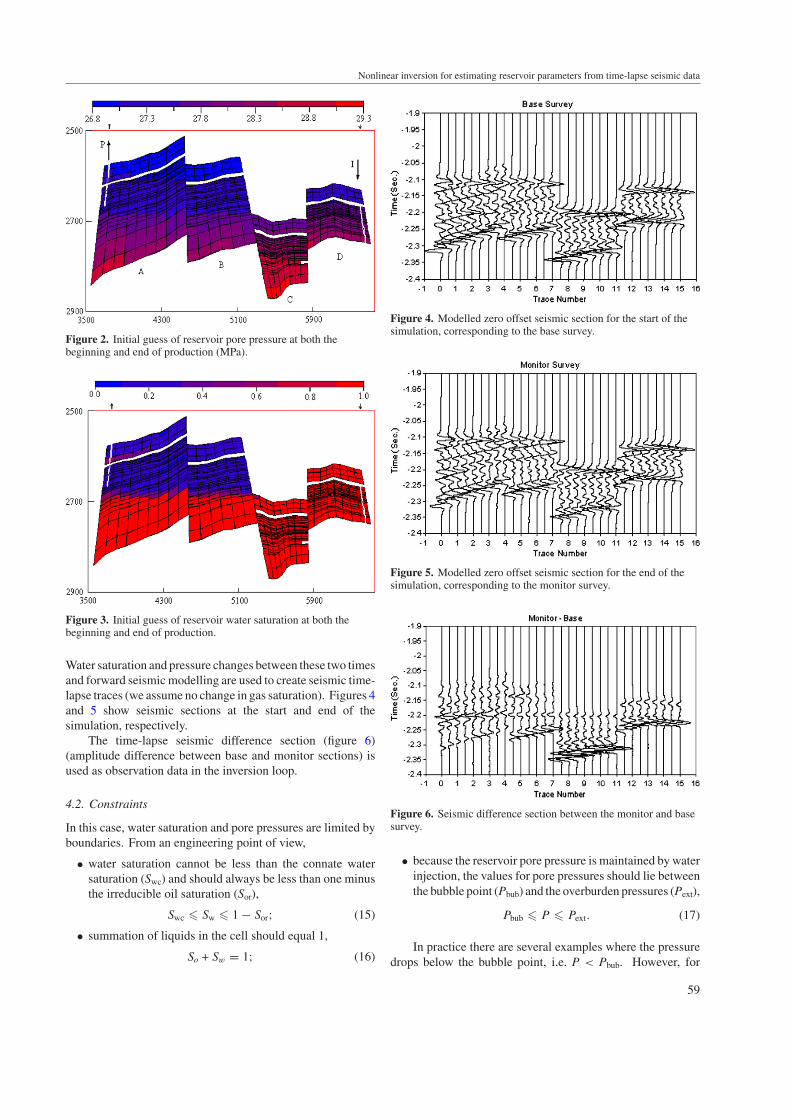
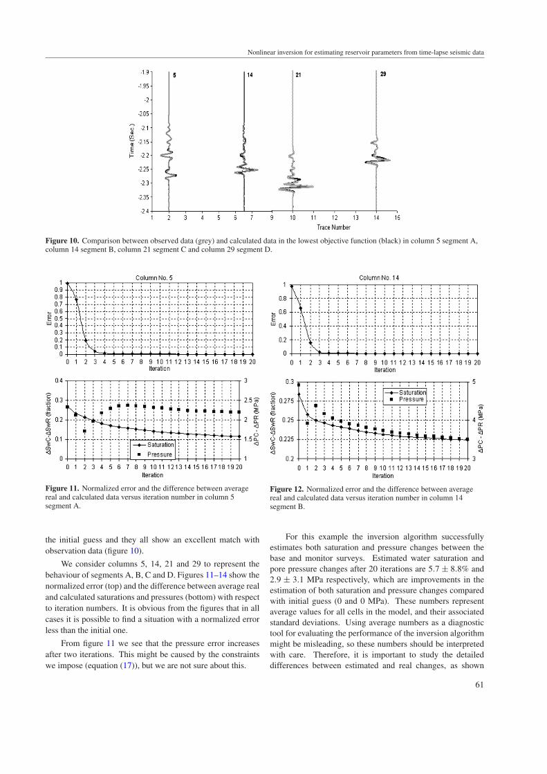
Figure 10. Comparison between observed data (grey) and calculated data in the lowest objective function (black) in column 5 segment A,column 14 segment B, column 21 segment C and column 29 segment D.

Figure 11. Normalized error and the difference between averagereal and calculated data versus iteration number in column 5segment A.

the initial guess and they all show an excellent match withobservation data (figure 10).

We consider columns 5, 14, 21 and 29 to represent thebehaviour of segments A, B, C and D. Figures 11–14 show thenormalized error (top) and the difference between average realand calculated saturations and pressures (bottom) with respectto iteration numbers. It is obvious from the figures that in allcases it is possible to find a situation with a normalized errorless than the initial one.

From figure 11 we see that the pressure error increasesafter two iterations. This might be caused by the constraintswe impose (equation (17)), but we are not sure about this.

Figure 12. Normalized error and the difference between averagereal and calculated data versus iteration number in column 14segment B.

For this example the inversion algorithm successfullyestimates both saturation and pressure changes between thebase and monitor surveys. Estimated water saturation andpore pressure changes after 20 iterations are 5.7 ± 8.8% and2.9 ± 3.1 MPa respectively, which are improvements in theestimation of both saturation and pressure changes comparedwith initial guess (0 and 0 MPa). These numbers representaverage values for all cells in the model, and their associatedstandard deviations. Using average numbers as a diagnostictool for evaluating the performance of the inversion algorithmmight be misleading, so these numbers should be interpretedwith care. Therefore, it is important to study the detaileddifferences between estimated and real changes, as shown

61

M Dadashpour et al

Figure 13. Normalized error and the difference between averagereal and calculated data versus iteration number in column 21segment C.

Figure 14. Normalized error and the difference between averagereal and calculated data versus iteration number in column 29segment D.

in figures 15 and 16. We notice that the pressure changeestimates for segments C and D are very good and agreevery well with the correct pressure changes. This is probablycaused by the fact that there are no saturation changes withinthese two segments (as shown in figure 16). For segments Aand B, however, the deviations between estimated and correctpressure changes are significant, especially for the middlelayers in segment A. Also the estimated saturation changes

Figure 15. Real and calculated changes in reservoir pore pressure(MPa).

Figure 16. Real and calculated changes in reservoir water saturation(fractions).

show significant deviations compared to the correct values,especially for segment B we observe an underestimation ofthe saturation changes close to the oil–water contact.

This degree of errors varies from segment to segment.Segments A and B show a good improvement in the estimationof water saturation changes with respect to the initial guess(15.5 ± 19.9% and 8.1 ± 12.2% for segments A and Brespectively). All segments except segment A show a good

62

Nonlinear inversion for estimating reservoir parameters from time-lapse seismic data

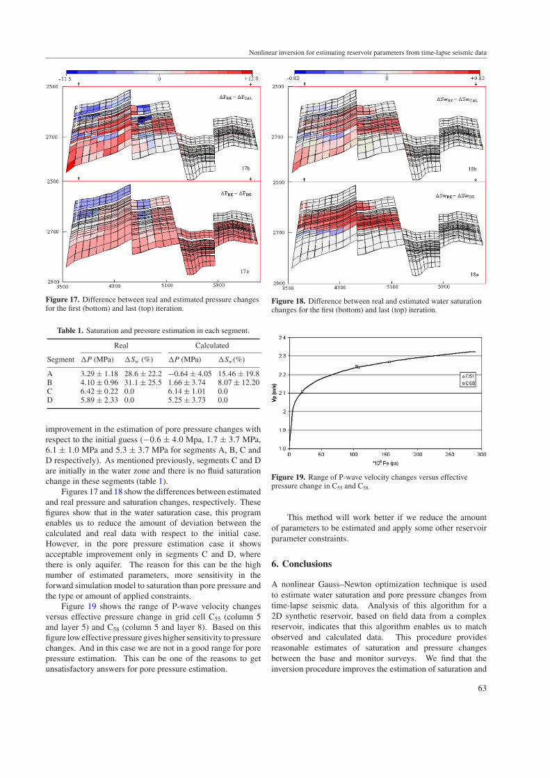
Figure 17. Difference between real and estimated pressure changesfor the first (bottom) and last (top) iteration.

Table 1. Saturation and pressure estimation in each segment.

Real Calculated

Segment �P (MPa) �Sw (%) �P (MPa) �Sw(%)

A 3.29 ± 1.18 28.6 ± 22.2 −0.64 ± 4.05 15.46 ± 19.8B 4.10 ± 0.96 31.1 ± 25.5 1.66 ± 3.74 8.07 ± 12.20C 6.42 ± 0.22 0.0 6.14 ± 1.01 0.0D 5.89 ± 2.33 0.0 5.25 ± 3.73 0.0

improvement in the estimation of pore pressure changes withrespect to the initial guess (−0.6 ± 4.0 Mpa, 1.7 ± 3.7 MPa,6.1 ± 1.0 MPa and 5.3 ± 3.7 MPa for segments A, B, C andD respectively). As mentioned previously, segments C and Dare initially in the water zone and there is no fluid saturationchange in these segments (table 1).

Figures 17 and 18 show the differences between estimatedand real pressure and saturation changes, respectively. Thesefigures show that in the water saturation case, this programenables us to reduce the amount of deviation between thecalculated and real data with respect to the initial case.However, in the pore pressure estimation case it showsacceptable improvement only in segments C and D, wherethere is only aquifer. The reason for this can be the highnumber of estimated parameters, more sensitivity in theforward simulation model to saturation than pore pressure andthe type or amount of applied constraints.

Figure 19 shows the range of P-wave velocity changesversus effective pressure change in grid cell C55 (column 5and layer 5) and C58 (column 5 and layer 8). Based on thisfigure low effective pressure gives higher sensitivity to pressurechanges. And in this case we are not in a good range for porepressure estimation. This can be one of the reasons to getunsatisfactory answers for pore pressure estimation.

Figure 18. Difference between real and estimated water saturationchanges for the first (bottom) and last (top) iteration.

Figure 19. Range of P-wave velocity changes versus effectivepressure change in C55 and C58.

This method will work better if we reduce the amountof parameters to be estimated and apply some other reservoirparameter constraints.

6. Conclusions

A nonlinear Gauss–Newton optimization technique is usedto estimate water saturation and pore pressure changes fromtime-lapse seismic data. Analysis of this algorithm for a2D synthetic reservoir, based on field data from a complexreservoir, indicates that this algorithm enables us to matchobserved and calculated data. This procedure providesreasonable estimates of saturation and pressure changesbetween the base and monitor surveys. We find that theinversion procedure improves the estimation of saturation and

63

M Dadashpour et al

pressure changes. For our test example, we find that the fluidsensitivity is somewhat larger than the sensitivity for porepressure changes.

Major weaknesses of the developed algorithm are thestrong dependence on the initial model (common for mostinversion techniques) and the strong need for constraints tolimit the solution space.

Another future step for this methodology will be toinclude the fluid simulation loop into the algorithm. Withthis extension, we will estimate reservoir properties suchas permeability and porosity distributions from time-lapseseismic data.

Acknowledgments

We thank the Norwegian University of Science andTechnology (NTNU), The Research Council of Norway andTOTAL for financial support. We also thank Alexey Stovasfor preparing the seismic forward modelling. We would like toextend our gratitude to Jan Ivar Jensen from NTNU for his helpduring this study. We are grateful to STATOIL and speciallyMagne Lygren for making it possible to use data from a realreservoir. We are also grateful to Schlumberger-GeoQuest forthe use of the Eclipse simulator. One anonymous revieweris acknowledged for constructive comments and numeroussuggestions that improved the paper.

Appendix A. Gauss–Newton optimization techniques

A.1. Theory of the Gauss–Newton algorithm

The theoretical anomaly expression of equations, which ismentioned in forward modelling, is nonlinear with respect tothe target parameters; therefore, the problem can be solved bythe least-squares inversion method.

The main assumptions in these kinds of algorithms are asfollows:

• The objective function is smooth.• It is possible to compute ∇F .

The condition for optimization is

F(�α0 + �α) < F(�α0), (A.1)

�α = ρ �p, (A.2)

where �α is the amount of perturbation of the function F(α),�p is the unit vector that provides a direction for descent and ρ

is a positive scalar that provides the step size.It is always possible to find a positive value of ρ that

results in reduction of the value of F provided that �p satisfiesthe following condition:

∇F �p < 0. (A.3)

where �p is defined as the sufficient descent direction and when�p satisfies the condition in equation (A.3).

The structure of the gradient algorithm synthesizes asfollows:

• Compute a sufficient descent direction (�p).

• Compute an adequate step size (ρ).

At each iteration of the Gauss–Newton algorithm, a linearsystem of equations is solved:

H�α = −∇F, (A.4)

where ∇F is the objective function and H is a symmetricand non-singular matrix. In the Gauss–Newton optimizationtechnique, it is considered as an approximation to the exactHessian matrix.

When equation (10) is used ∇F and H for Gauss–Newtonoptimization techniques will be calculated from the following:

∇F = −2J T (dobs − dcal), (A.5)

H = 2J T J, (A.6)

where J is the Jacobian matrix which is the first derivativeof time dependent reservoir properties to static reservoirproperties, which is also referred to as sensitivity coefficientand it will be explained further in appendix A.2.

The inversion process continues until the error betweenthe observed and the calculated data is less than a certain errornumber by controlling either the RMS value or the normalizedvalue.

A.2. Jacobian matrix

A Jacobian matrix is a first-order partial derivative of time-dependent reservoir properties (seismic amplitudes in thiscase) with respect to static reservoir parameters (saturationand pressure in this case). It is used to find the linearapproximation of a system of differential equations. Theexpressions for partial derivatives are usually obtained byanalytical differentiation in the inversion process.

By definition the partial derivative is the derivative withrespect to a single variable of a function of two or morevariables, regarding other variables as constants. In the presentstudy, the numerical Jacobian matrix is made by the calculationof the partial derivative with respect to saturation (α1) andpressure (α2) in each cell. In the general form of first-orderfinite differences, the derivation of any function f (α) at a pointαi (i = 1, . . . , N) is given by the following equation:

∂f (α)

∂αi

= f (αi + �α) − f (α)

�α. (A.7)

In this case, the partial derivative of amplitudes that iscalculated from forward modelling with respect to the reservoirparameters (saturation and pressure in each cell), can becalculated as

∂dcalj

∂α1= dcal

j (αi + �α) − d(α)

�α, (A.8)

df calj

∂αnop= dcal

j (αi + �α) − d(α)

�α. (A.9)

64

Nonlinear inversion for estimating reservoir parameters from time-lapse seismic data

The final Jacobian matrix will be

J ≡ ∂ �dcal

∂ �α =

⎡⎢⎢⎢⎢⎢⎢⎢⎢⎢⎢⎢⎣

∂dcal1

∂ �α1

∂dcal1

∂ �α2. .

∂dcal1

∂ �αnpar

∂dcal2

∂ �α1. . . .

. . . . .

. . . . .

∂dcalnobs

∂ �α1. . .

∂dcalnobs

∂ �αnpar

⎤⎥⎥⎥⎥⎥⎥⎥⎥⎥⎥⎥⎦

. (A.10)

For computing partial derivatives for each iteration, theperturbation values for each parameter are taken as 1% of thatvalue (�αi = 0.01αi, i = 1, . . . , nop).

Appendix B. Normalized RMS (NRMS)

Normalized RMS (NRMS) is defined as the RMS of thedifference between two datasets divided by the average ofthe RMS of each dataset (Kragh and Christie 2002):

NRMS(%) = 200RMS(ai − bi)

RMS(ai) + RMS(bi), (B.1)

where RMS is defined as

RMS(xi) =√∑ (

x2i

)N

. (B.2)

N is the number of samples in the summation interval. NRMSis expressed as a percentage and ranges from 0% to 200%.

If two datasets are identical, then NRMS is 0%. If twodatasets are completely different, then NRMS is 200%. Ifboth datasets are random noise, then NRMS is 141% (thesquare root of 2). NRMS is very sensitive to static, phase oramplitude differences. If one dataset is a phase-shifted versionof the other, then NRMS for a 10◦ phase shift is 17.4%, for a90◦ phase shift is 141% and for a 180◦ phase shift is 200%. Ifone dataset is a scaled version of the other, then NRMS for a0.5 scale is 66.7%.

References

Aanonsen S I, Aavatsmark I, Barkve T, Cominelli A, Gonard R,Gosselin O, Kolasinski M and Reme H 2003 Effect of scaledependent data correlations in an integrated history matchingloop combining production data and 4D seismic data, SPE79665 SPE Reservoir Simulation Symp. (Houston, USA, 3–5February)

Behrens R, Condon P, Haworth W, Bergeron M, Wang Z andEcker C 2002 4D seismic monitoring of water influx at baymarchand: the practical use of 4D in an imperfect world SPEReservoir Eval. Eng. 5 410–20

Burkhart T, Hoover A R and Flemings P B 2000 Time-lapse (4D)seismic monitoring of primary production of turbiditereservoirs as South Timbalier Block 295, offshore Louisiana,Gulf of Mexico Geophysics 65 351–67

Christensen N and Wang H F 1985 The influence of pore pressureand confining pressure on dynamic elastic properties of Bereasandstone Geophysics 50 207–13

Domenico S N 1974 Effect of water saturation on seismic reflectivityof sand reservoirs encased in shale Geophysics 39 759–69

Eastwood J, Lebel J P, Dilay A and Blakeslee S 1994 Seismicmonitoring of steam-based recovery of bitumen The LeadingEdge 4 242–51

Gassmann F 1951 Elastic wave through a packing of spheresGeophysics 16 673–85

Gill P E, Murray W and Wright M H 1981 Practical Optimization(New York: Academic)

Haskell N A 1953 The dispersion of surface waves in multilayeredmedia Bull. Seismol. Soc. Am. 43 17–34

Helgesen J and Landrø M 1993 Estimation of elastic parametersfrom AVO effects in the tau-p domain Geophys. Prospect.41 341–66

Kennett B L N 1983 Seismic Wave Propagation in Stratified Media(Cambridge: Cambridge University Press)

Kragh E and Christie P 2002 Seismic repeatability, normalizedRMS and predictability The Leading Edge 21 640–7

Kretz V, Le Ravalec-Dupin M and Roggero F 2004 An integratedreservoir characterization study matching production data and4D seismic SPE Reservoir Eva. Eng. 7 116–22

Landa J L 1979 Reservoir parameter estimation constrained topressure transients, performance history and distributedsaturation data PhD Dissertation Stanford University

Landa J and Horne R 1997 A procedure to integrate well test data,reservoir performance history and 4-D seismic information intoa reservoir descriptions, SPE 38653 SPE Ann. Tech. Conf.Exhibition (San Antonio, TX, 5–8 October)

Landa J L, Kamal M M, Jenkins C D and Home R N 1996 Reservoircharacterization constrained to well test data: a field example,SPE 36511 SPE Ann. Tech. Conf. Exhibition (Dallas, USA, 6–9October)

Landrø M, Digranes P and Strønen L K 2001 Mapping reservoirpressure and saturation changes using seismic methods—possibilities and limitations First Break 19 671–7

Landrø M 2001 Discrimination between pressure and fluidsaturation changes from time-lapse seismic data Geophysics66 836–44

Landrø M, Solheim O A, Hilde E, Ekren B O and Strønen L K 1999The Gullfaks 4D seismic study Pet. Geosc. 5 213–26

Lazaratos S K and Marion B P 1997 Croswell seismic imaging ofreservoir changes caused by CO2 injection The LeadingEdge 16 1300–7

Lepine O J, Bissell R C, Aanonsen S I and Barker J W 1998Uncertainty analysis in predictive reservoir simulation usinggradient information, SPE 48997 SPE Ann. Tech. Conf.Exhibition (LA, USA, 27–30 September)

Mantica S, Cominelli A and Mantica G 2001 Combining global andlocal optimization techniques for automatic history matchingproduction and seismic data, SPE 66355 SPE Res. SimulationSymp. (Houston, TX, USA, 11–14 February)

Mavko G, Mukerji T and Dvorkin J 1998 The Rock PhysicsHandbook (Cambridge: Cambridge University Press)

Mindlin R D 1949 Compliance of elastic bodies in contact, App.Mech. 16 259–68

Nur A 1989 Four-dimensional seismology and (true) directdetection of hydrocarbon The Leading Edge 8 30–6

Reuss A 1929 Berechnung der fliessgrense von mishkristallenZ. Angew. Math. Mech. 9 49–58

Schulze-Riegert R W, Axmann J K, Haase O, Rian D T and You Y2001 Optimization methods for history matching of complexreservoirs, SPE 66393 SPE Reservoir Simulation Symp.(Houston, USA, 11–14 February)

Slater G E and Durrer E J 1971 Adjustment of reservoir simulationmodels to match field performance Soc. Petroleum Eng. J. 11295–305

Stovas A M and Arntsen B 2006 Vertical propagation oflow-frequency waves in finely layered mediaGeophysics 71 87–94

Stovas A M and Landrø M 2005 Fluid-pressure discrimination inanisotropic reservoir rocks—a sensitivity studyGeophysics 70 1–11

Tan T B 1995 A computational efficient Gauss–Newton method forautomatic history matching, SPE 29100 SPE Symp. ReservoirSimulation (San Antonio, USA, 12–15 February)

65

M Dadashpour et al

Thomas L K, Hellums L J and Reheis J M 1971 Nonlinearautomatic history-matching technique for reservoir simulatormodels, SPE 3495 SPE-AIME 46th Ann. Fall Meeting (NewOrleans, USA, 3–6 October)

Van Ditzhuijzen R, Oldenziel T and Van Kruijsdijk C 2001Geological parameterization of a reservoir model for history

matching incorporating time-lapse seismic based on a casestudy of the Statfjord field, SPE 71318 SPE Ann. Tech. Conf.Exhibition (New Orleans, LA, USA, 30 September–3 October)

Vidal S 2000 Integrating geomechanics and geophysics for reservoirseismic monitoring feasibility studies, SPE 65157 SPE Ann.Tech. Conf. Exhibition (Paris, France)

66