estimating primaries by sparse inversion in a curvelet ... · estimating primaries by sparse...

SLIMUniversity of British Columbia

Tim T.Y. Lin and Felix J. Herrmann

Estimating Primaries by Sparse Inversion in a Curvelet-like Representation Domain

Thursday, June 16, 2011

SLIM

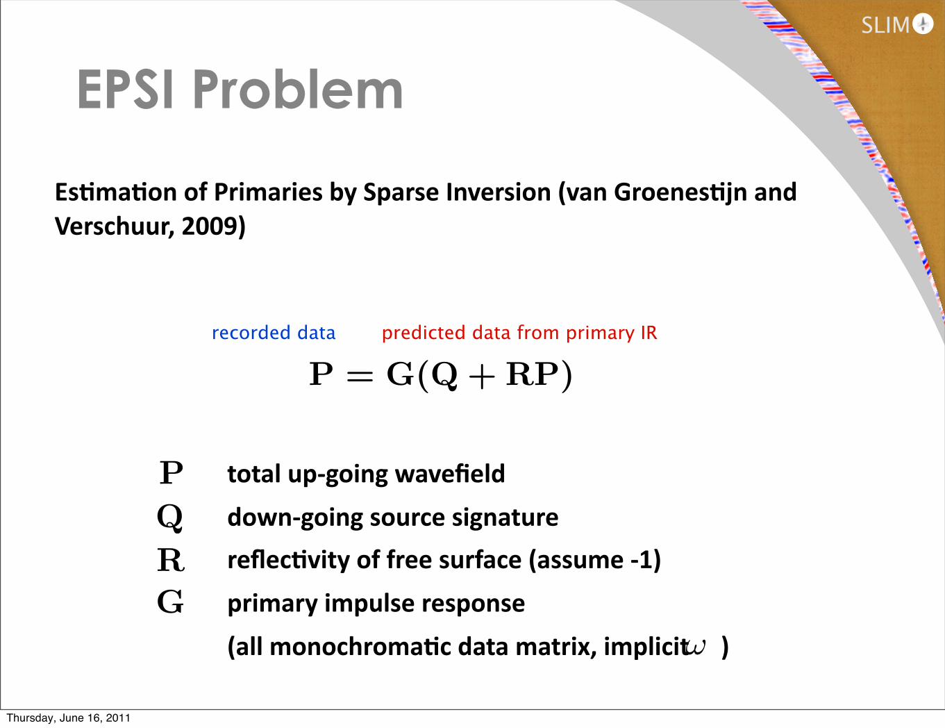
Es#ma#on of Primaries by Sparse Inversion (van Groenes#jn and Verschuur, 2009)

EPSI Problem

total up-‐going wavefield

down-‐going source signature

reflec#vity of free surface (assume -‐1)

primary impulse response

(all monochroma#c data matrix, implicit )

R

ω

PQ

recorded data predicted data from primary IR

P = G(Q + RP)

G


SLIM

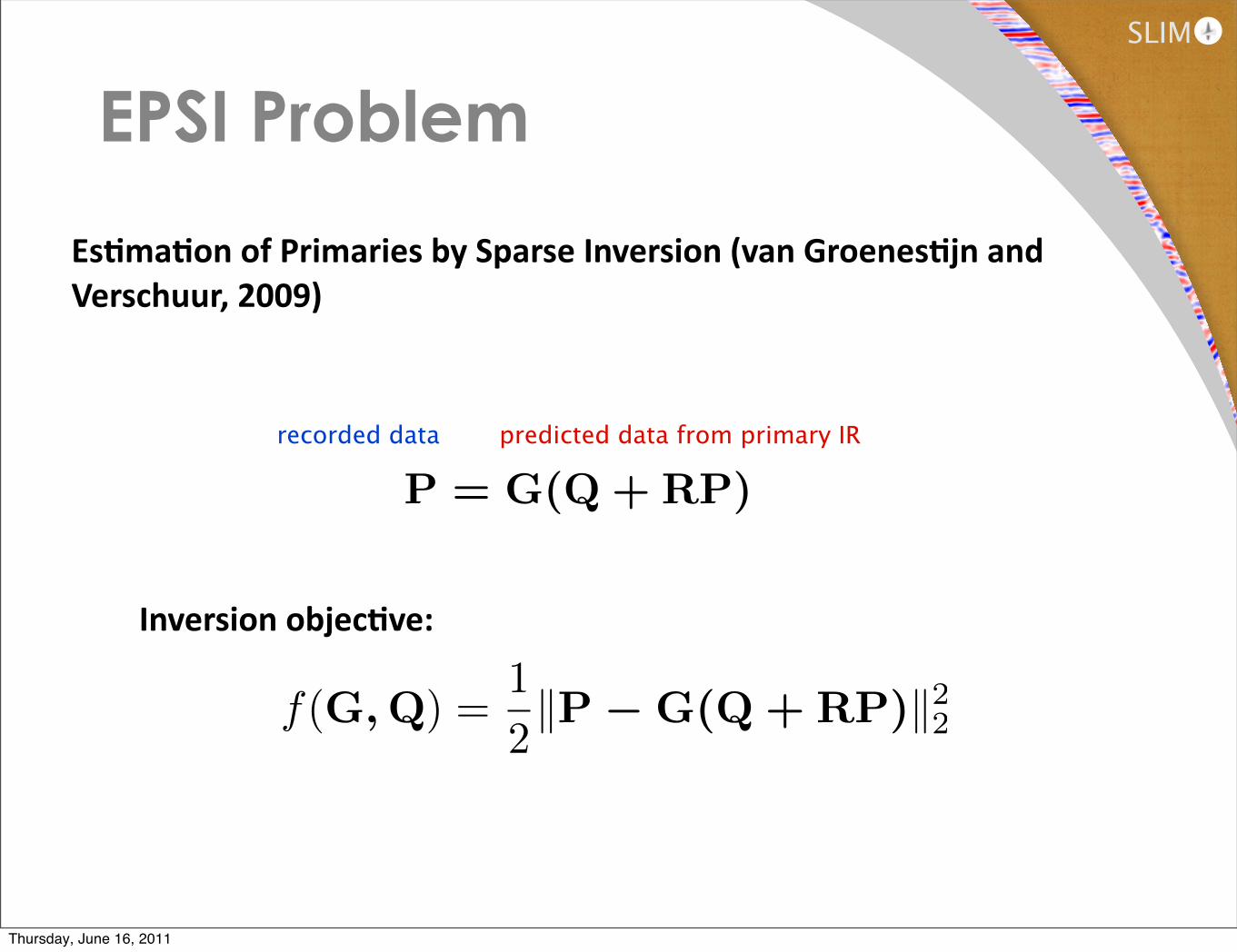
Es#ma#on of Primaries by Sparse Inversion (van Groenes#jn and Verschuur, 2009)


P = G(Q + RP)

Inversion objec#ve:

EPSI Problem

f(G,Q) =1

2�P − G(Q + RP)�22


SLIM

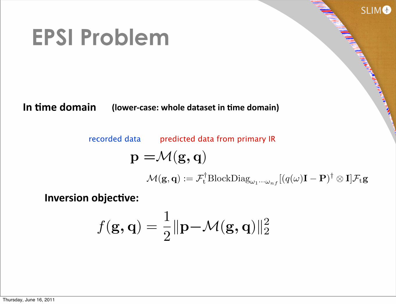
In #me domain


Inversion objec#ve:

p =M(g, q)

(lower-‐case: whole dataset in 2me domain)

M(g,q) := F†tBlockDiagω1···ωnf

[(q(ω)I−P)† ⊗ I]Ftg

f(g, q) =1

2�p−M(g, q)�22

EPSI Problem


SLIM

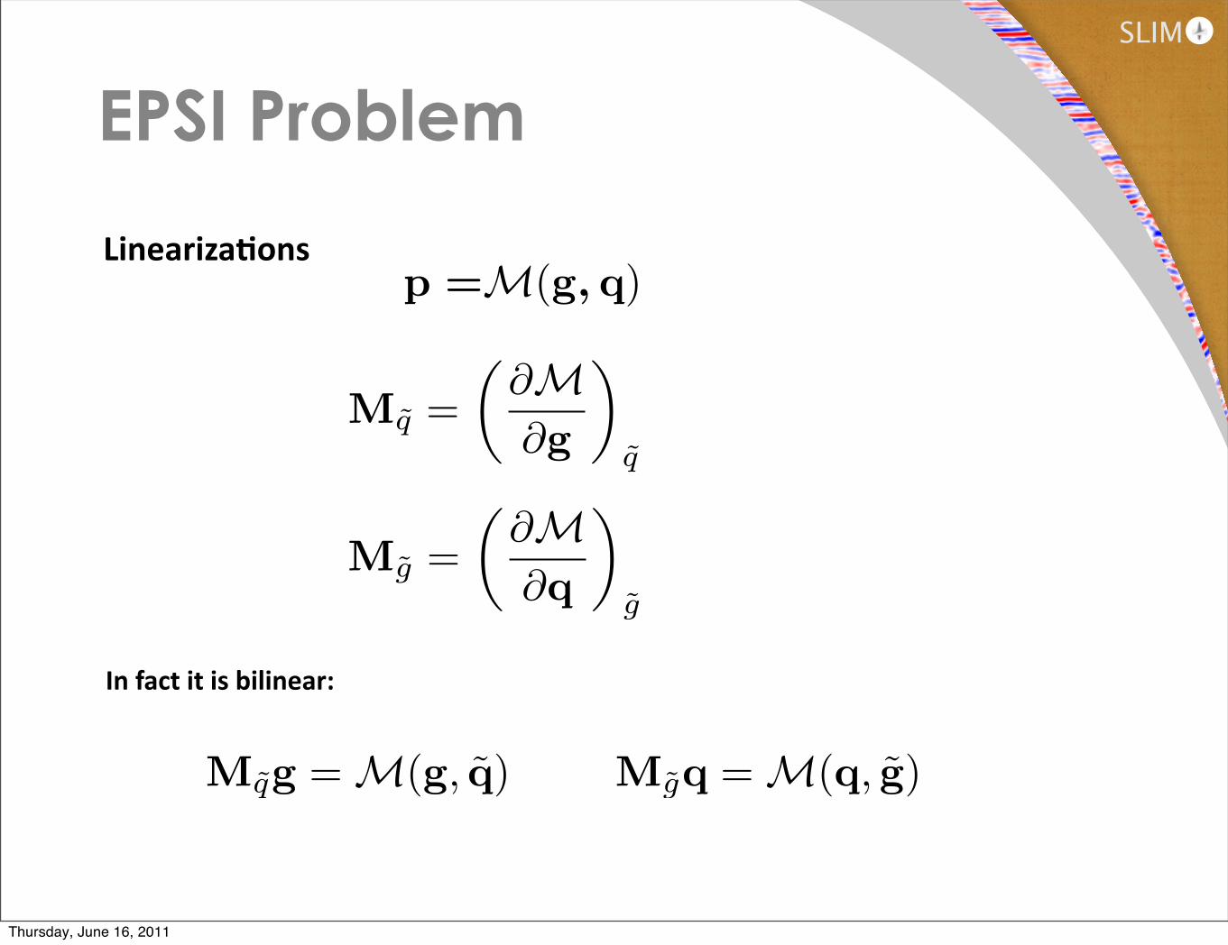
Lineariza#ons

EPSI Problem

Mq̃g = M(g, q̃) Mg̃q = M(q, g̃)

In fact it is bilinear:

Mq̃ =

�∂M∂g

�

q̃

Mg̃ =

�∂M∂q

�

g̃

p =M(g, q)


SLIM

Lineariza#ons

EPSI Problem

Associated objec#ves:

Mq̃ =

�∂M∂g

�

q̃

Mg̃ =

�∂M∂q

�

g̃

p =M(g, q)

fq̃(g) =1

2�p−Mq̃g�22 fg̃(q) =

1

2�p−Mg̃q�22


SLIM

Do:

EPSI Procedure

gk+1 = gk + α∇fqk(gk)

qk+1 = qk + β∇fgk+1(qk)

Alterna2ng updates (Gauss-‐Sidel) to the linearized problem


SLIM

EPSI Procedure

Gradient sparsity

S : pick largest ρ elements per trace

gk+1 = gk + αS(∇fqk(gk))


Do:


SLIM


SLIM

Related to two underlying sub-‐problems:

EPSI Procedure

ming

�p−Mq̃g�2 s.t. nnz(g) ≤ ρ

minq

�p−Mg̃q�2

Which approximates:

minq

�p−Mg̃q�2

ming

nnz(g) s.t. �p−Mq̃g�2 ≤ σ(no#on of sparsest solu#on)


SLIM

EPSI Procedure

Can be made non-‐combinatorial (convex) by:

minq

�p−Mg̃q�2(minimum L1 solu#on usually the sparsest solu#on)

ming

�g�1 s.t. �p−Mq̃g�2 ≤ σ


SLIM

Convex EPSI


Do:

gk+1 = gk + α SoftThφ(∇fqk(gk))

So?-‐thresholding solves an L1 minimiza2on problem, but how is

determined?

φ


SLIM

Copyright © by SIAM. Unauthorized reproduction of this article is prohibited.

894 EWOUT VAN DEN BERG AND MICHAEL P. FRIEDLANDER

Projected gradient. Our application of the SPG algorithm to solve (LS! ) followsBirgin, Mart́ınez, and Raydan [5] closely for the minimization of general nonlinearfunctions over arbitrary convex sets. The method they propose combines projected-gradient search directions with the spectral step length that was introduced by Barzilaiand Borwein [1]. A nonmonotone line search is used to accept or reject steps. Thekey ingredient of Birgin, Mart́ınez, and Raydan’s algorithm is the projection of thegradient direction onto a convex set, which in our case is defined by the constraintin (LS! ). In their recent report, Figueiredo, Nowak, and Wright [27] describe theremarkable e!ciency of an SPG method specialized to (QP"). Their approach buildson the earlier report by Dai and Fletcher [18] on the e!ciency of a specialized SPGmethod for general bound-constrained quadratic programs (QPs).

2. The Pareto curve. The function ! defined by (1.1) yields the optimal valueof the constrained problem (LS! ) for each value of the regularization parameter " .Its graph traces the optimal trade-o" between the one-norm of the solution x andthe two-norm of the residual r, which defines the Pareto curve. Figure 2.1 shows thegraph of ! for a typical problem.

The Newton-based root-finding procedure that we propose for locating specificpoints on the Pareto curve—e.g., finding roots of (1.2)—relies on several importantproperties of the function !. As we show in this section, ! is a convex and di"erentiablefunction of " . The di"erentiability of ! is perhaps unintuitive, given that the one-norm constraint in (LS! ) is not di"erentiable. To deal with the nonsmoothness ofthe one-norm constraint, we appeal to Lagrange duality theory. This approach yieldssignificant insight into the properties of the trade-o" curve. We discuss the mostimportant properties below.

2.1. The dual subproblem. The dual of the Lasso problem (LS! ) plays aprominent role in understanding the Pareto curve. In order to derive the dual of(LS! ), we first recast (LS! ) as the equivalent problem

(2.1) minimizer,x

!r!2 subject to Ax + r = b, !x!1 " ".

0 1 2 3 4 5 6 70

5

10

15

20

25

one!norm of solution

two!

norm

of r

esid

ual

Fig. 2.1. A typical Pareto curve (solid line) showing two iterations of Newton’s method. Thefirst iteration is available at no cost.

Feasible

Pareto curve

Pareto curve

(van den Berg, Friedlander, 2008)

Look at the solu2on space and the line of op2mal solu2ons (Pareto curve)

minimize �x�1subject to �Ax− b�2 ≤ σ








(2.1) minimizer,x


0 1 2 3 4 5 6 70

5

10

15

20

25


two!

norm

of r

esid

ual


σ

�x�1feasible solu2on with smallest

Pareto curve










(2.1) minimizer,x


0 1 2 3 4 5 6 70

5

10

15

20

25


two!

norm

of r

esid

ual


Deriva2ve given by

Pareto curve



�ATr�∞


Pareto curve





Trace #

Tim

e

50 100 150 200 250

(a) Image with missing traces

Trace #50 100 150 200 250

(b) Interpolated image

0 0.5 1 1.5 20

50

100

150

200

250

one!norm of solution (x104)

two

!no

rm o

f re

sidua

l

Pareto curveSolution path

(c) Pareto curve and solution path

Fig. 6.1. Corrupted and interpolated images for problem seismic. Graph (c) shows the Paretocurve and the solution path taken by SPGL1.

ever, as might be expected of an interior-point method based on a conjugate-gradientlinear solver, it can require many matrix-vector products.

It may be progressively more di!cult to solve (QP!) as ! ! 0 because the reg-ularizing e"ect from the one-norm term tends to become negligible, and there is lesscontrol over the norm of the solution. In contrast, the (LS" ) formulation is guaranteedto maintain a bounded solution norm for all values of " .

6.4. Sampling the Pareto curve. In situations where little is known aboutthe noise level #, it may be useful to visualize the Pareto curve in order to understandthe trade-o"s between the norms of the residual and the solution. In this sectionwe aim to obtain good approximations to the Pareto curve for cases in which it isprohibitively expensive to compute it in its entirety.

We test two approaches for interpolation through a small set of samples i =1, . . . , k. In the first, we generate a uniform distribution of parameters !i = (i/k)"ATb"!and solve the corresponding problems (QP!i). In the second, we generate a uni-form distribution of parameters #i = (i/k)"b"2 and solve the corresponding problems(BP#i). We leverage the convexity and di"erentiability of the Pareto curve to approx-imate it with piecewise cubic polynomials that match function and derivative valuesat each end. When a nonconvex fit is detected, we switch to a quadratic interpolation

minimize �Ax− b�2subject to �x�1 ≤ τ

solve with SPG(spectral projected gradients)


SLIM

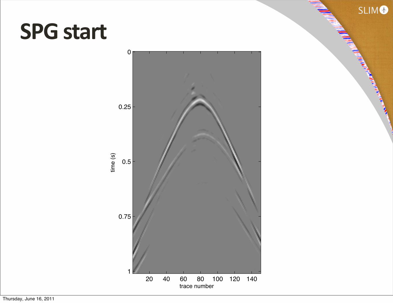
SPG start

trace number

time

(s)

20 40 60 80 100 120 140

0

0.25

0.5

0.75

1


SLIM

trace number

time

(s)

20 40 60 80 100 120 140

0

0.25

0.5

0.75

1

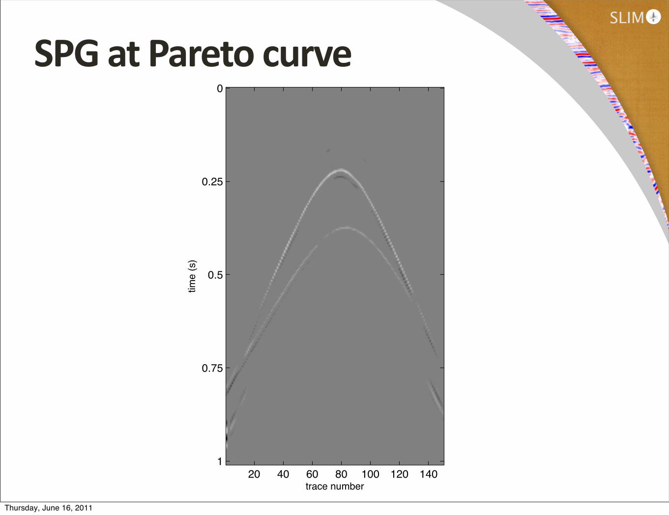
SPG at Pareto curve


Pareto curve

Only solve least-‐squares matching for q when solu2on reaches Pareto curve




Trace #

Tim

e

50 100 150 200 250

(a) Image with missing traces

Trace #50 100 150 200 250

(b) Interpolated image

0 0.5 1 1.5 20

50

100

150

200

250

one!norm of solution (x104)

two

!no

rm o

f re

sidua

l

Pareto curveSolution path

(c) Pareto curve and solution path

Fig. 6.1. Corrupted and interpolated images for problem seismic. Graph (c) shows the Paretocurve and the solution path taken by SPGL1.

ever, as might be expected of an interior-point method based on a conjugate-gradientlinear solver, it can require many matrix-vector products.

It may be progressively more di!cult to solve (QP!) as ! ! 0 because the reg-ularizing e"ect from the one-norm term tends to become negligible, and there is lesscontrol over the norm of the solution. In contrast, the (LS" ) formulation is guaranteedto maintain a bounded solution norm for all values of " .

6.4. Sampling the Pareto curve. In situations where little is known aboutthe noise level #, it may be useful to visualize the Pareto curve in order to understandthe trade-o"s between the norms of the residual and the solution. In this sectionwe aim to obtain good approximations to the Pareto curve for cases in which it isprohibitively expensive to compute it in its entirety.

We test two approaches for interpolation through a small set of samples i =1, . . . , k. In the first, we generate a uniform distribution of parameters !i = (i/k)"ATb"!and solve the corresponding problems (QP!i). In the second, we generate a uni-form distribution of parameters #i = (i/k)"b"2 and solve the corresponding problems(BP#i). We leverage the convexity and di"erentiability of the Pareto curve to approx-imate it with piecewise cubic polynomials that match function and derivative valuesat each end. When a nonconvex fit is detected, we switch to a quadratic interpolation

minimize �Ax− b�2subject to �x�1 ≤ τ


SLIM

Robust EPSI procedure

While

(Solve with SPGL1 un#l Pareto curve reached)

gk+1 = argming

�p−Mqkg�2 s.t. �g�1 ≤ τk

determine new τk from the Pareto curve

qk+1 = argminq

�p−Mgk+1q�2(Solve with LSQR)

�p−M(gk,qk)�2 > σ


SLIM

REPSI in transform domain

Modify just the problem for g:

minq

�p−Mg̃q�2

ming

�g�1 s.t. �p−Mq̃g�2 ≤ σ


SLIM


Modify just the problem for g:

minq

�p−Mg̃q�2

S : sparsifying representation for seismic signals

S† : synthesis operator for S

-‐ Should have spa2ally localized support-‐ ex: nd-‐Wavelets, Curvelets, etc...

(basis pursuit)minx

�x�1 s.t. �p−Mq̃S†x�2 ≤ σ, g = S†x


SLIM


While

(Solve with SPGL1 un#l Pareto curve reached)

determine new τk from the Pareto curve

qk+1 = argminq

�p−Mgk+1q�2(Solve with LSQR)

xk+1 = argminx

�p−MqkS†x�2 s.t. �x�1 ≤ τk

gk+1 = S†xk+1

�p−M(gk,qk)�2 > σ


SLIM

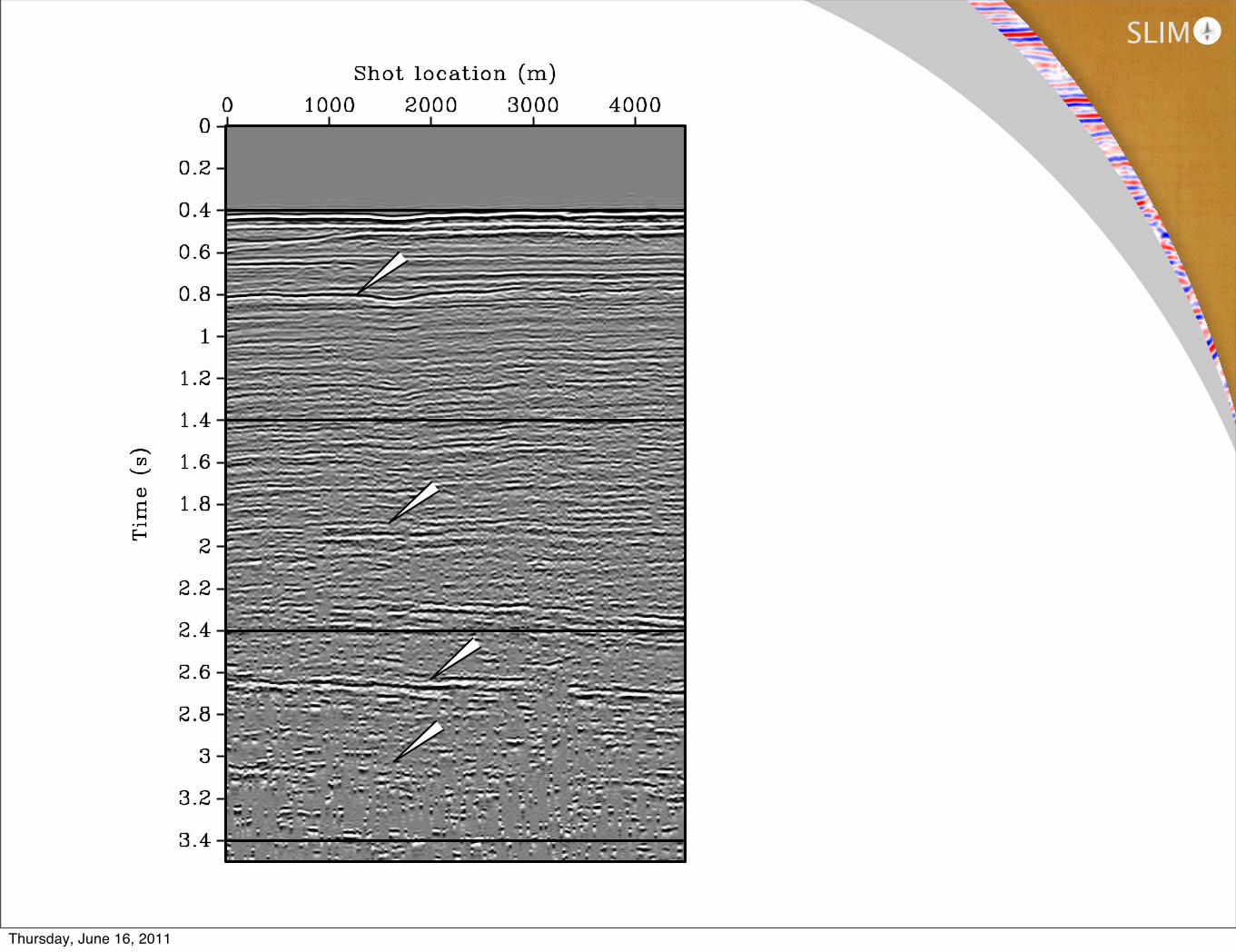
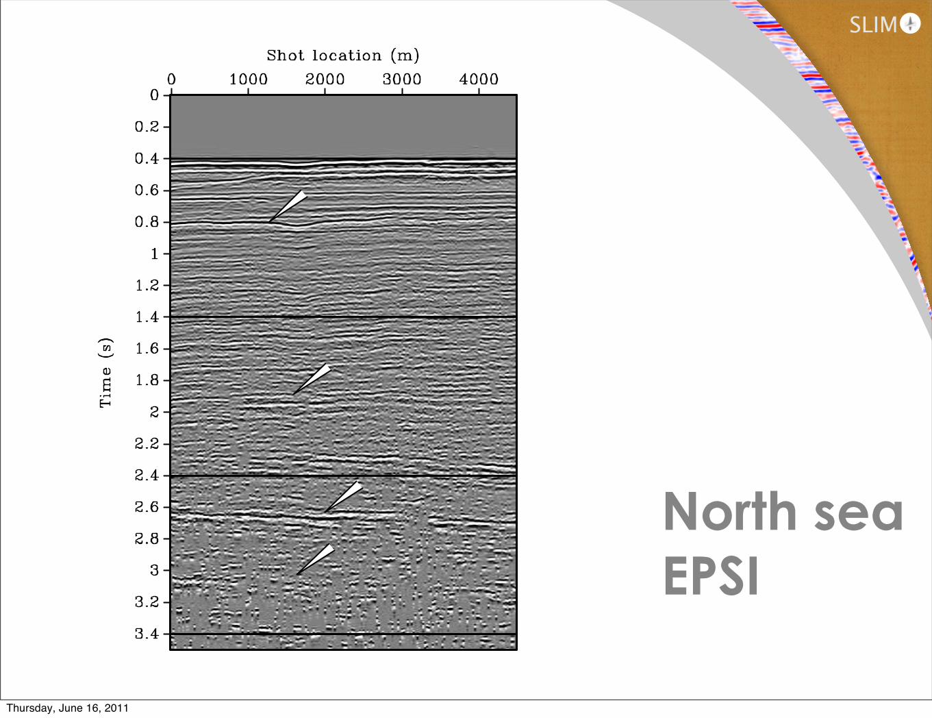
North seaEPSI


SLIM

North seaEPSI + Sp


SLIM

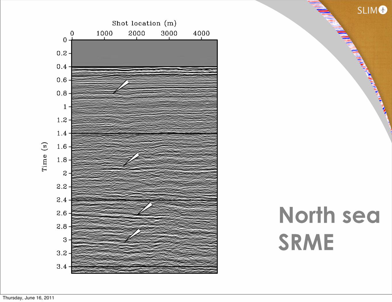
North seaSRME


SLIM

North seadata


SLIM

North seapred. mul


SLIM

(show Gulf of Suez results here)


SLIM

• L1-‐convexification behaves nicely and has few free parameters

• Follows the Pareto curve into a series of projected gradient problems

• Easily incorporates seeking the solution in a transform domain that promotes continuity

summary


Acknowledgements

This work was in part financially supported by the Natural Sciences and Engineering Research Council of Canada Discovery Grant (22R81254) and the Collaborative Research and Development Grant DNOISE II (375142-‐08). This research was carried out as part of the SINBAD II project with support from the following organizations: BG Group, BP, Chevron, ConocoPhillips, Petrobras, Total SA, and WesternGeco.

SLIM

Special thanks to G.J. van Groenes#jn, Eric Verschuur, and the rest of the members of DELPHI

M. Friedlander and E. van den Berg


SLIM

Chapter 6: EPSI and near offset reconstruction: marine data applications 6 – 3

a) b) c) d) e) f)

Fig. 6.1 A schematic illustration of the relations between primaries and multiples. a) A shot gather

taken from a dataset with one single reflector. b) The primary event in the shot gather is

the consequence of fi ring the source. c) The up-going data will reflect at the surface and

generate the multiples. The same multiples are obtained when in each receiver location a

secondary source is present, which is fi red at the time the primary event reaches the receiver.

These secondary sources of the primary event are depicted as stars. d) The multiples are the

result of adding all the delayed primaries. e) The same shot gather as in (a). The shaded

area indicates the offset gap in the data. f) The fi rst order multiple is built from delayed

primaries caused by secondary sources. The secondary source inside the missing data gap

has not been measured but its consequences have an effect outside the gap.

that the near offsets are not measured and, thus, need to be interpolated before the multiple

prediction process is applied. This means that wrongly interpolated near offsets will pro-

duce errors in the predicted multiples and, therefore, limit the quality of the primary output.

van Groenestijn and Verschuur (2009b) demonstrates that EPSI can use the multiples to re-

construct the missing near offsets. Therefore, EPSI performs well on estimating primaries on

shallow water data. An other data-driven reconstruction method is the pseudo primary method

(Shan and Guitton, 2004) where a multidimensional auto correlation of the data is used to fill

the near offset gap. Curry and Shan (2008) improved the pseudo primary method by extending

it with prediction error filters. However, this improvement does not exclude cross correlation

artefacts from the missing near offsets completely.

After reviewing the EPSI method, we will discuss the role of the residual when we apply

EPSI to a moderately deep water marine dataset. Next, we will review the modified EPSI

method that is able to reconstruct missing near offset data simultaneously with estimating the

primaries. This algorithm is applied to a shallow water marine dataset. The result is compared

with iterative SRME applied to the same dataset with interpolated near offsets.

6.2 The primary-multiple model and iterative SRME

In the detail-hiding operator notation for 2D data (Berkhout, 1982) a bold quantity represents

a pre-stack data volume for one frequency; columns represent monochromatic shot records

(van Groenes#jn and Verschuur 08)Thursday, June 16, 2011

estimating primaries by sparse inversion in a curvelet ... · estimating primaries by sparse...

Documents