The impact of causality on information-theoretic

source and channel coding problems

Harikrishna R Palaiyanur

Electrical Engineering and Computer SciencesUniversity of California at Berkeley

Technical Report No. UCB/EECS-2011-55

http://www.eecs.berkeley.edu/Pubs/TechRpts/2011/EECS-2011-55.html

May 13, 2011

Copyright © 2011, by the author(s).All rights reserved.

Permission to make digital or hard copies of all or part of this work forpersonal or classroom use is granted without fee provided that copies arenot made or distributed for profit or commercial advantage and that copiesbear this notice and the full citation on the first page. To copy otherwise, torepublish, to post on servers or to redistribute to lists, requires prior specificpermission.

The impact of causality on information-theoretic source and channel codingproblems

by

Harikrishna R. Palaiyanur

A dissertation submitted in partial satisfaction of the

requirements for the degree of

Doctor of Philosophy

in

Engineering — Electrical Engineering and Computer Sciences

in the

Graduate Division

of the

University of California, Berkeley

Committee in charge:

Professor Anant Sahai, ChairProfessor Kannan Ramchandran

Professor Jim Pitman

Spring 2011

The impact of causality on information-theoretic source and channel codingproblems

Copyright 2011by

Harikrishna R. Palaiyanur

1

Abstract

The impact of causality on information-theoretic source and channel coding problems

by

Harikrishna R. Palaiyanur

Doctor of Philosophy in Engineering — Electrical Engineering and Computer Sciences

University of California, Berkeley

Professor Anant Sahai, Chair

This thesis studies several problems in information theory where the notion of causalitycomes into play. Causality in information theory refers to the timing of when information isavailable to parties in a coding system.

The first part of the thesis studies the error exponent (or reliability function) for severalcommunication problems over discrete memoryless channels. In particular, it studies anupper bound to the error exponent, or equivalently, a lower bound to the error probabilityof general codes, called the Haroutunian exponent. The Haroutunian exponent is the bestknown upper bound to the error exponent for two channel coding problems: fixed blocklengthcoding with feedback and fixed delay coding without feedback. For symmetric channels likethe binary symmetric channel and the binary erasure channel, the Haroutunian exponentevaluates to the sphere-packing exponent, but for asymmetric channels like the Z-channel,the Haroutunian exponent is strictly larger than the sphere-packing exponent. The reason forthe presumed looseness of the Haroutunian exponent is that it assumes, despite the inherentcausality of feedback, a code might be able to predict future channel behavior based onpast channel behavior and accordingly tune its input distribution. Intuitively, this kind ofnoncausal information should not be available to an encoder when the channel is memoryless.While we have not been able to tighten the Haroutunian exponent to the sphere-packingexponent for fixed blocklength codes with feedback, we describe some attempts made atbridging the gap. Additionally, we describe how to tighten the upper bound for two caseswhen the encoder is somehow limited: if the encoding strategy is constrained to use fixedtype inputs regardless of output sequence and if there is a delay in the feedback path. Thelatter of these results leads to the insight that the Haroutunian exponent of a parallel channelconstructed of independent uses of the original asymmetric channel approaches the sphere-packing exponent of the original channel after normalization. This fact can then be used toshow that the error exponent for fixed delay codes is upper bounded by the sphere-packingexponent.

The second part of the thesis studies lossy compression of the arbitrarily varying sourcesintroduced by Berger in his paper entitled ‘The Source Coding Game’. An arbitrarily varying

2

source is a model for a source that samples other subsources under the control of an agentcalled a switcher. Motivated by compression of active vision sources, we seek upper and lowerbounds for the rate-distortion function of an arbitrarily varying source when the switcherhas noncausal knowledge about the realizations of the subsources it samples from. We findthat when the subsources are memoryless, noncausal knowledge of subsource realizations isstrictly better than information about past subsource realizations only.

i

To Amma, Appa and Sarah.

ii

Contents

1 Introduction 11.1 What could noncausal feedback do? . . . . . . . . . . . . . . . . . . . . . . . 31.2 Contributions . . . . . . . . . . . . . . . . . . . . . . . . . . . . . . . . . . . 10

2 The Haroutunian exponent for block coding with feedback 132.1 Introduction . . . . . . . . . . . . . . . . . . . . . . . . . . . . . . . . . . . . 132.2 Definitions and notation . . . . . . . . . . . . . . . . . . . . . . . . . . . . . 312.3 The sphere-packing and Haroutunian bounds . . . . . . . . . . . . . . . . . . 312.4 Failed Approaches to proving the sphere-packing bound for codes with feedback 352.5 Sphere-packing holds when the fixed type encoding tree condition holds . . . 452.6 What needs to be proved for sphere-packing to hold for fixed-length codes

with feedback? . . . . . . . . . . . . . . . . . . . . . . . . . . . . . . . . . . 482.7 Delayed feedback is not useful for very large delays . . . . . . . . . . . . . . 532.8 The Haroutunian exponent for a parallel channel . . . . . . . . . . . . . . . 592.9 Limited memory at the encoder means the sphere-packing bound holds . . . 612.10 Concluding remarks . . . . . . . . . . . . . . . . . . . . . . . . . . . . . . . . 64

3 Tightening to sphere-packing for fixed delay coding without feedback 663.1 Introduction . . . . . . . . . . . . . . . . . . . . . . . . . . . . . . . . . . . . 663.2 Fixed delay coding and anytime codes . . . . . . . . . . . . . . . . . . . . . 693.3 Control and anytime coding . . . . . . . . . . . . . . . . . . . . . . . . . . . 723.4 Problem setup . . . . . . . . . . . . . . . . . . . . . . . . . . . . . . . . . . . 743.5 Tightening to sphere-packing for fixed delay codes . . . . . . . . . . . . . . . 763.6 A weaker result for anytime codes . . . . . . . . . . . . . . . . . . . . . . . . 783.7 Concluding remarks . . . . . . . . . . . . . . . . . . . . . . . . . . . . . . . . 83

4 Lossy compression of arbitrarily varying sources 854.1 Introduction . . . . . . . . . . . . . . . . . . . . . . . . . . . . . . . . . . . . 854.2 Problem Setup . . . . . . . . . . . . . . . . . . . . . . . . . . . . . . . . . . 894.3 R(D) for the cheating switcher . . . . . . . . . . . . . . . . . . . . . . . . . 934.4 Noisy observations of subsource realizations . . . . . . . . . . . . . . . . . . 95

iii

4.5 The helpful switcher . . . . . . . . . . . . . . . . . . . . . . . . . . . . . . . 974.6 Examples . . . . . . . . . . . . . . . . . . . . . . . . . . . . . . . . . . . . . 984.7 Computing R(D) for an AVS . . . . . . . . . . . . . . . . . . . . . . . . . . 1034.8 Concluding remarks . . . . . . . . . . . . . . . . . . . . . . . . . . . . . . . . 108

5 Conclusion 110

A Block coding appendix 113A.1 Definitions and notation for Chapter 2 . . . . . . . . . . . . . . . . . . . . . 113A.2 Sphere-packing without feedback via method of types . . . . . . . . . . . . . 117A.3 Sphere-packing without feedback via change of measure . . . . . . . . . . . . 120A.4 Haroutunian exponent for fixed-length codes with feedback . . . . . . . . . . 125A.5 A special family of test channels . . . . . . . . . . . . . . . . . . . . . . . . . 128A.6 Failed Approaches to proving the sphere packing bound for codes with feedback134A.7 Sheverdyaev’s proof . . . . . . . . . . . . . . . . . . . . . . . . . . . . . . . . 144A.8 Augustin’s manuscript . . . . . . . . . . . . . . . . . . . . . . . . . . . . . . 151A.9 Sphere packing holds when the fixed type encoding tree condition holds . . . 153A.10 Limited memory at the encoder means the sphere packing bound holds . . . 161A.11 Equivalent statements . . . . . . . . . . . . . . . . . . . . . . . . . . . . . . 165A.12 Delayed feedback . . . . . . . . . . . . . . . . . . . . . . . . . . . . . . . . . 169A.13 The Haroutunian exponent of a parallel channel . . . . . . . . . . . . . . . . 175A.14 Lemmas for block codes . . . . . . . . . . . . . . . . . . . . . . . . . . . . . 179

B Fixed delay coding appendix 191B.1 Proof of Theorem 8 . . . . . . . . . . . . . . . . . . . . . . . . . . . . . . . . 191B.2 The Z-Channel . . . . . . . . . . . . . . . . . . . . . . . . . . . . . . . . . . 205

C Arbitrarily varying sources appendix 214C.1 The cheating switcher with clean observations . . . . . . . . . . . . . . . . . 214C.2 Adversarial switching with noisy observations . . . . . . . . . . . . . . . . . 218C.3 Uniform continuity of R(p,D) . . . . . . . . . . . . . . . . . . . . . . . . . . 223C.4 Proof of Lemma 10 . . . . . . . . . . . . . . . . . . . . . . . . . . . . . . . . 226

Bibliography 227

iv

Acknowledgments

I do not have the required faculty with words to express how grateful I am to have beenadvised by Anant Sahai, but I will try anyway. I have never met someone who combinessuch great technical horsepower with raw, unbridled passion for research. Additionally,Anant possesses a remarkable intellectual curiosity about the workings of the world that hasrubbed off on me to some extent. When I came to Berkeley, I believed from my undergraduateeducation that being able to solve problems was the most important skill needed to doresearch. Over my time as a graduate student, Anant taught me that being able to askquestions was as important, if not more important, for conducting research. As a student ofAnant’s, I received all-encompassing training to improve my presentation, communicationand writing skills. In a good way, Anant never let me feel as if there was not room forimprovement, and I thank him for that. There were many times in my graduate careerwhen I would get stalled or frustrated by the slow pace of progress I was making. Anantwas always patient and encouraging, especially during these periods of high stress and lowproductivity. There were so many meetings with him, after which I would feel reinvigoratedto tackle problems that I had almost given up on. It was here at Berkeley, with the help ofAnant, that I developed the capability to ‘just keep moving forward’.

In the course of my time at Berkeley, I have also been fortunate to have some wonder-ful collaborators. Interactions with Baris Nakiboglu of MIT sparked some of the channelcoding investigations in the thesis. Cheng Chang helped quite a bit in the early versionsof the source coding material. I also worked with Pulkit Grover, Kris Woyach and RahulTandra on interesting topics not included in the thesis. I would like to thank Professors Kan-nan Ramchandran, Michael Gastpar and Jim Pitman for serving on the Qualifying Examcommittee and their useful comments. Professor Pitman’s Stat 205 A and B courses wereextremely useful for developing the probabilistic maturity needed to do research in informa-tion theory. I would also like to thank Cheng Chang, Gireeja Ranade and Pulkit Grover forreading chapters of the thesis. I also appreciate the late Sergio Servetto for introducing meto research in information theory when I was at Cornell.

Obviously, I would never even be at an institution as fine as Berkeley if it were not for myfamily. As a child, it is hard to appreciate how one’s parents make decisions and sacrificesthat profoundly affect one’s future. I thank my parents, Ravi and Sumathi, for their loveand support throughout my life. I also thank them for instilling in me a love for learning andappreciation for education at an early age. The song ‘Everybody’s Free (To Wear Sunscreen)’by Baz Luhrmann has a lyric that has stuck with me. It says “your choices are half chance,so are everybody else’s”. I take two cautionary messages from this lyric: don’t be so quickto judge others for their plights and don’t accept that all fortunes gained in your lifetimewere derived from your own efforts. One thing you don’t get to choose in life is your parents,and I got some great ones. I also got an OK brother. Just kidding, Shyam, I love you too.My grandparents also showered me with love and encouragement. Chengalpattu1 Thatha

1For some reason, I never dropped the childhood habit of adding a geographical location as an adjective

v

gave me a formidable nose to face the world with and I wish I knew him through morethan just photos. KK Nagar Patti taught me the utility of discipline and consistency. KKNagar Thatha’s affection and enthusiasm for life and the simple pleasures was infectious.Finally, my lone living grandparent, Chengalpattu (now Ekkatuthangal) Patti has been ahuge inspiration, and is someone I can talk to for hours. I am so happy to make her proudby becoming, in her words, the first Ph.D. in the family.

Life at Berkeley has not been all about work. Since its inception, the people of WirelessFoundations have made it a wonderful place to work, think, talk and laugh. These peopleinclude(d), in no particular order, Dan Hazen, Sameer Vermani (who taught me to cook afew dishes), Amin Gohari, John Secord, Bobak Nazer (my social hour partner and fellowcookie connoisseur), Krish Eswaran, Anand Sarwate (the mother bear of WiFo, in an en-dearing way), Alex Dimakis, Cheng Chang (my pool playing partner), Rahul Tandra (mydiligent workout buddy), Mubaraq Mishra, Galen Reeves (my trusted cubiclemate), GuyBresler (who gave me some amazing pep talks), Kris Woyach, Gireeja Ranade, Se-YongPark, Jiening Zhan, Jonathan Tsao, Venky Ekambaram, Sameer Pawar, Salim El Rouay-heb, Parv Venkitasubramaniam, Sahand Neghaban, Dapo Omidiran (my pickup basketballbuddy) and Pulkit Grover (the meanest guy I ever met, just kidding). My friends fromhigh school, Nikhil Kothari, Arjun Banker and Sravi Chennupati, who became Bay Areatransplants as well, were always good for a fun overnight trip to the city. To anyone I forgot,I apologize, but I certainly appreciate your friendship.

I fell in love with basketball as an undergrad, but I became addicted to it at the RSFin Berkeley. One of the things that made me feel like a part of the EECS community wasplaying intramural basketball with people from across the department: Alessandro Abate(who graciously invited me to play on the team after I sent a blind email to the department),Alvise Boniventi, Nate Pletcher (a true Indiana ballplayer), Dapo Omidiran, Eric Battenberg,Galen Reeves, Marshall Miller, Simone Gambini, Matt Pierson, Alessandro Uccelli, SandeepMohan and even Professor Seth Sanders. Thanks for the fun and competition guys.

Last, but certainly not least, I want to thank my girlfriend, Sarah Kloss. Her orthogonalpursuits have been a constant reminder that the world is much bigger and more beautifulthan what I know and experience. More importantly, her unconditional love and supportare priceless.

Finally, I would like to gratefully acknowledge the National Science Foundation for finan-cial support of the research in this thesis, first in the form of a Graduate Research Fellowshipand second in the form of grants when I was a GSR.

to a relationship for my grandparents.

1

Chapter 1

Introduction

In a theory of information, it is not surprising that the idea of causality naturally arises.This is because the utility of knowledge is based on many factors: what is learned, how muchit costs, who learns it (i.e., what actions can they carry out with the information) and whenthe knowledge is learned. The last factor, the timing of when knowledge is learned, is thesubject of this thesis.

In the popular vernacular, the concept of causality is about cause and effect. In the socialand physical sciences, effects are observed and correlated with hypothetical causes, and oneof the goals of science is to show that a hypothesized cause is actually causative of the effect.A related meaning is the idea that before one event happens, a different one must occur first.This meaning of causality is related to the causality in the information theoretic problemsin this thesis. We will study source and channel coding problems where actions of agents inthe problems are taken with varying levels of knowledge of the realizations of certain randomvariables in the problems. The amount of knowledge available before these actions are takenwill determine whether we think of the problems as having a causal or noncausal nature.

The first part of the thesis continues the study of error exponents for point-to-pointchannel coding. In point-to-point channel coding, as shown in Figure 1.1, an encoder wishesto communicate a message over a noisy communication medium called a channel to a decoder.The message is assumed to be uniformly random from a finite set and the encoder maps themessage to input symbols for the channel. The channel randomly (noisily) maps the channelinput symbol to a channel output symbol according to a known conditional probabilitydistribution, W (y|x). The encoder has a certain number of uses of the channel (calledblocklength) to communicate the message to the decoder reliably (with low probability oferror). Shannon, in his seminal paper [1] launching the field of information theory, showedthat there is a critical quantity called the capacity of the channel, C(W ), that determineshow much information can be communicated reliably across the channel. He showed thecapacity can be calculated as

C(W ) = maxP

I(P,W ),

2

Encoder DecoderW(y|x)M M

>

1,2,...,2 nR

Block length n

X (M)i

Yi

DMC

Figure 1.1: Fixed blocklength coding over a discrete memoryless channel W (y|x). The rateof communication is R bits per channel use, and the blocklength is n, so the message isuniformly drawn from one of exp(nR) possibilities.

where P is a distribution on the input of the channel and I(P,W ) denotes the mutualinformation between the input and output of the channel W when the input distribution is P .The operational meaning of the capacity of the channel is that if the rate of communication(measured in bits communicated per use of the channel) is less than the capacity, there arecodes that communicate the message with arbitrarily low probability of error in the limit oflarge blocklengths.

Because large blocklengths also correspond to large delay, one would also like to knowhow large a blocklength is needed to achieve a desired reliability while communicating at agiven rate over the channel. The study of error exponents seeks to answer this question byanalyzing the probability of error for optimal codes with a given blocklength and rate. Itcan be shown that for optimal codes,

P(Error) ' e−nE(R),

where n is the blocklength and E(R) is the error exponent at rate R. One finds lower boundsto E(R) by proving upper bounds to error probability for specific codes and upper boundsto E(R) by finding lower bounds to error probability for general codes.

The first part of the thesis explores the noncausal interpretation of one upper bound,called the Haroutunian bound, to the error exponent for several variants of the communica-tion problem just described. The original problem where the Haroutunian exponent appearsis channel coding with casual output feedback. Shannon showed [2] that even if the en-coder is given knowledge of the realizations of previous channel outputs before choosing achannel input at each time, the capacity of the (discrete, memoryless) channel is unchanged.Haroutunian [3] proved an upper bound to the error exponent for fixed blocklength codeswith feedback that suffers from a technical weakness: it assumes that causal feedback allowsthe encoder to predict future channel behavior based on past channel behavior. The boundassumes that this knowledge can then be acted on by the encoder to improve error perfor-mance by optimizing its input distribution using this noncausal knowledge of the channelbehavior it will face. This fact only makes the bound weak for asymmetric channels (chan-nels for which the uniform input distribution is not optimal in some sense). The weaknessof the bound lies in the fact that for memoryless channels, past channel behavior cannot beused to predict future channel behavior. Thus, the Haroutunian bound appears to grant the

3

encoder with feedback a power it does not in reality possess. A more precise introductionto the problem is given in Chapter 2, but suffice to say for now that Chapters 2 and 3 aredevoted to disallowing this possibliity that such noncausal knowledge could be learned bythe code in several channel coding problems where the Haroutunian bound arises.

The second part of the thesis deals with lossy compression of arbitrarily varying sources(AVSs). Arbitrarily varying sources are used to model sources which output data that isactually a processed or dynamically sampled version of other ‘subsources’, as shown in Figure1.2. An agent with some knowledge about the realizations and distributions of the subsourcescontrols the processing or sampling operation. The concept of an arbitrarily varying sourcewas introduced by Berger in his paper “The Source Coding Game” [4]. The source codinggame is a game played between two players, a coder and a switcher. The coder is tryingto lossily compress the output of the AVS to a specified distortion. The switcher is theagent in control of which subsource is sampled at each time, and in the game, is trying tomake life difficult for the coder by forcing the coder to use as high a rate as possible. Inthis version of the game, the switcher is an adversary to the coder. Berger characterizes therate-distortion function when the switcher is adversarial and has strictly causal knowledge ofthe realizations of memoryless subsources. That is, the switcher must set the switch positionbefore learning of the subsource realizations at the current time. Berger asks the questionof whether ‘noncausal’ knowledge of the subsource realizations can be used by the switcherto increase the rate-distortion function. It is this question that we answer in Chapter 4,both for the adversarial model of the switcher studied by Berger and a ‘helpful’ model weintroduce, where the switcher is actually trying to help the coder use less rate.

In both parts of the thesis, we will model subsources and channels as discrete, memorylesssystems. The impact of causality will then come through by how varying levels of knowledgefor the agent in the two problems can shape the relevant controlled distributions. In thechannel coding problem, the encoder is the agent in control of the output of the channel byusing its input distribution as a ‘control’ input. In the source coding problem, the switcheris the agent in control of the output distribution of the AVS by using its knowledge of thesubsource realizations and distributions to decide how to sample the subsource.

1.1 What could noncausal feedback do?

To get a glimpse of what can happen when we look at differing levels of causality in aninformation-theoretic problem, let us think of channel coding with feedback. The mainweakness of the Haroutunian bound is that it assumes that causal output feedback can allowthe encoder to tune its input distribution by predicting future channel behavior (becauseit is difficult to prove otherwise). Thus, the causal output feedback is giving some kind of‘precognitive’ knowledge of future channel behavior. Why is this something to be afraid ofto begin with, from the point of view of understanding fundamental behavior of optimalcodes? One might guess that knowledge of the channel behavior at the encoder only is not

4

p1

p2

pm

x1,1 x1,2, ,

x2,1 x2,2, ,

xm,1 xm,2, ,

x , x ,...1 2

Figure 1.2: An arbitrarily varying source whose output symbol at each time is the output ofone of a finite number of ‘subsources’. In Berger’s paper [4] and this thesis, the subsources areassumed to be discrete, memoryless and stationary. The switcher decides which subsources’symbol will be output based on the knowledge it has, which may be noncausal.

1 1

0 0

1-

1-

Figure 1.3: The binary symmetric channel with crossover probability δ. The output Y is theinput X with probability 1− δ and is 1−X with probability δ.

enough to improve performance because the decoder is still unaware of the channel noise theencoder faced, and therefore the lack of synchronicity might render the noncausal knowledgeuseless. To dispel this notion, we look into some models of feedback that appear aphysicaland are noncausal, but do have applications in problems involving interference and storageon memories.

How does one begin to think of precognitive knowledge of channel behavior? For example,take the binary symmetric channel (BSC), shown in Figure 1.3, which flips its input withprobability δ < 1/2. The capacity of the BSC (without feedback or with causal outputfeedback) is 1 − hb(δ), where hb(δ) is the binary entropy function hb(δ) = −δ log δ − (1 −δ) log(1− δ). One model for the BSC is that the output Y is the modulo-2 sum of the inputX an an independent Bernoulli random variable Z with parameter δ, Yi = Xi ⊕ Zi. Inthis model, if the encoder knows the value of Zi in a procognitive way before inputting Xi,clearly the capacity is 1 bit per channel use, which is larger than 1− hb(δ). But this is not

5

the only model for noise in the BSC. Consider a ‘noisy packet drop’ model for the BSC. LetZi be a Bernoulli process with parameter 2δ and Yi an independent Bernoulli process withparameter 1/2. Then, let the output of the channel be

Yi = Xi(1− Zi) + YiZi.

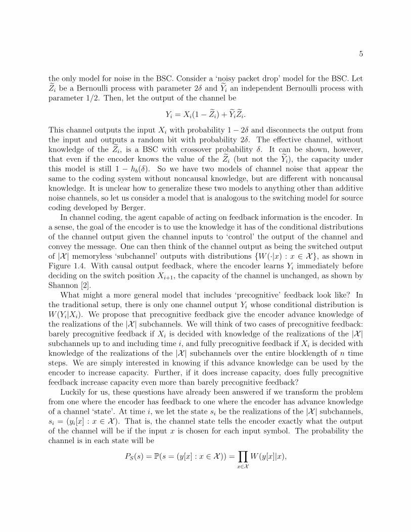
This channel outputs the input Xi with probability 1− 2δ and disconnects the output fromthe input and outputs a random bit with probability 2δ. The effective channel, withoutknowledge of the Zi, is a BSC with crossover probability δ. It can be shown, however,that even if the encoder knows the value of the Zi (but not the Yi), the capacity underthis model is still 1 − hb(δ). So we have two models of channel noise that appear thesame to the coding system without noncausal knowledge, but are different with noncausalknowledge. It is unclear how to generalize these two models to anything other than additivenoise channels, so let us consider a model that is analogous to the switching model for sourcecoding developed by Berger.

In channel coding, the agent capable of acting on feedback information is the encoder. Ina sense, the goal of the encoder is to use the knowledge it has of the conditional distributionsof the channel output given the channel inputs to ‘control’ the output of the channel andconvey the message. One can then think of the channel output as being the switched outputof |X | memoryless ‘subchannel’ outputs with distributions W (·|x) : x ∈ X, as shown inFigure 1.4. With causal output feedback, where the encoder learns Yi immediately beforedeciding on the switch position Xi+1, the capacity of the channel is unchanged, as shown byShannon [2].

What might a more general model that includes ‘precognitive’ feedback look like? Inthe traditional setup, there is only one channel output Yi whose conditional distribution isW (Yi|Xi). We propose that precognitive feedback give the encoder advance knowledge ofthe realizations of the |X | subchannels. We will think of two cases of precognitive feedback:barely precognitive feedback if Xi is decided with knowledge of the realizations of the |X |subchannels up to and including time i, and fully precognitive feedback if Xi is decided withknowledge of the realizations of the |X | subchannels over the entire blocklength of n timesteps. We are simply interested in knowing if this advance knowledge can be used by theencoder to increase capacity. Further, if it does increase capacity, does fully precognitivefeedback increase capacity even more than barely precognitive feedback?

Luckily for us, these questions have already been answered if we transform the problemfrom one where the encoder has feedback to one where the encoder has advance knowledgeof a channel ‘state’. At time i, we let the state si be the realizations of the |X | subchannels,si = (yi[x] : x ∈ X ). That is, the channel state tells the encoder exactly what the outputof the channel will be if the input x is chosen for each input symbol. The probability thechannel is in each state will be

PS(s) = P(s = (y[x] : x ∈ X )) =∏x∈X

W (y[x]|x),

6

W( |1).

W( | ).

y[1]

y[ ]

. . .

. . .Encoder Decoder

Input letter X

Message

. . .

Precognitive feedback

Y

Figure 1.4: A way of thinking of channels analogous to the arbitrarily varying source. Thechannel is composed of |X | subchannels, each of which produce symbols from the outputalphabet IID according to distributions W (·|x). The encoder then chooses which symbolis the output of the channel by selecting the input symbol. Without feedback, or with causalfeedback, the channel appears to the encoder and decoder to be a DMC with transitionprobabilities W (y|x). This model allows for a notion of ‘precognitive feedback’, where theencoder would be aware of the outputs of each of the subchannels before making a decisionon the input symbol.

where for simplicity, we have made the assumption that the subchannels are independentof each other. We note that other models for a DMC can be recovered by making thesubchannels correlated with each other (but independent over time). For example, theadditive noise model for the BSC has fully correlated subchannels, where either both inputsare flipped or neither input is flipped.

Without any feedback or only causal knowledge of the channel state, the encoder appearsto be facing a channel with conditional distribution W , because its knowledge of the outputof the channel for a given input symbol is just the conditional distribution. With precogni-tive feedback, it knows the state and therefore the output of the channel deterministicallygiven the input. Barely precognitive feedback then means that the encoder decides Xi withknowledge of (s1, . . . , si) and fully precognitive feedback means the encoder chooses Xi withknowledge of (s1, . . . , sn). The capacity for these ‘state knowledge’ problems was determinedby Shannon [5] in the barely precognitive case and Gelfand and Pinsker [6] in the fully pre-cognitive case. These are also called channel side-information problems because the encodergets side-information about the state of the channel before deciding on the input letter.However, in this precognitive feedback instance, the side-information is very special becausegiven the side-information of the channel state, the output is a deterministic function of theinput. The key insight of [5] is that, rather than thinking of inputs as being letters fromX , we think of inputs as being ‘strategies’, i.e., functions mapping an observed state to a

7

1 1

0 0

1 1

0 0

1

0 0

1 1

0

Flip Don't Flip Output 0 Output 1

Figure 1.5: The possible states the BSC can be in for the model in Figure 1.4.

channel input letter,

t : S → X .

In the case of barely precognitive feedback, the capacity as determined by Shannon is

Cbp = maxPT

I(T ;Y ),

where the joint distribution is

P(s, t, y) = PS(s)PT (t)1(y[t(s)] = y),

and I(T ;Y ) is the mutual information between the random variables T and Y . The notationy[x] denotes the component of s corresponding to the input x, which has marginal distribu-tion W (·|x). In the fully precognitive case, Gelfand and Pinsker showed that the capacityis

Cfp = maxPT |S

I(T ;Y )− I(T ;S),

where the joint distribution is

P(s, t, y) = PS(s)PT |S(t|s)1(y[t(s)] = y)

and the optimization is over conditional distributions of the strategy T , conditioned on thestate S.

Let us evaluate these capacities for two simple binary input, binary output channels: thebinary symmetric channel (BSC) and the Z-channel. For the BSC, at each time, the channelcan be in one of four states: flip both inputs with probability δ2, don’t flip the inputs withprobability (1−δ)2, output only 0 with probability δ(1−δ), or output only 1 with probabilityδ(1− δ) as shown in Figure 1.5.

When the state of the channel is ‘flip both inputs’ or ’don’t flip the inputs’, the encoderwith advance knowledge of the state can make the output of the channel be either 0 or 1. Inthe other states, the encoder is constrained to output the symbol that occurs as the realizationof both subchannels. It is inconsequential what a strategy does in these constrained states

8

0 0.1 0.2 0.3 0.4 0.50

0.2

0.4

0.6

0.8

1

Capa

city

(bi

ts/c

hann

el u

se)

Crossover probability of BSC

Fully precognitive

Causal feedback

Barely precognitive

Figure 1.6: Capacity of the BSC with no feedback, barely precognitive feedback and fullyprecognitive feedback as a function of the crossover probability δ ∈ [0, 1/2]. Fully precog-nitive feedback increases capacity over barely precognitive feedback, which in turn is largerthan capacity without feedback.

as it cannot affect the output of the channel. It can be shown that, with barely precognitivefeedback, the capacity of the channel is the capacity of a BSC with crossover probabilityδ(1− δ), which is less than δ. Thus

Cbp = 1− hb(δ(1− δ)) > 1− hb(δ).

In a paper that studies storage in memories with known defects, Heegard and El Gamal [7]show that with fully precognitive feedback, the encoder can communicate a bit for everytime instant that the state allows the output of the channel to be chosen, even though thedecoder does not know when these time instants occur. Thus,

Cfp = 1− 2δ(1− δ) > Cbp > 1− hb(δ).

Hence, we find that noncausal knowledge of channel behavior can indeed be used to increasecapacity. In the example of the BSC, the difference between barely precognitive feedbackand fully precognitive feedback is also an increase in capacity, as shown in Figure 1.6.

As another example, consider the Z-channel, a channel which faithfully transmits 0’s as0’s, but flips 1’s to 0’s with probability δ. Without feedback, or with causal output feedback,the capacity of the Z-channel with crossover probability δ is

CZ(δ) = hb (p∗(δ)(1− δ))− p∗(δ)hb(δ),

9

1 1

0 0

1

0 0

Flip Don't FlipFigure 1.7: The states that a Z-channel can be in. A 0 is always transmitted as a 0, but a 1can either be transmitted as a 1 or flipped to a 0.

where

p∗(δ) =

[(1− δ)

(1 + exp

(hb(δ)

1− δ

))]−1.

With precognitive feedback, the encoder is made to know in advance whether the channelwill flip an input of 1 to 0 or not, as shown in Figure 1.7. With barely precognitive feedback,it can be checked that the capacity is unchanged, i.e., Cbp = CZ(δ). With fully precognitivefeedback, the capacity actually increases to Cfp = 1− δ (bits per channel use), the fractionof time the channel output can be freely chosen to be either 0 or 1. Hence, for the Z-channel, knowledge of the channel state immediately before deciding the input does notincrease capacity (as shown in Figure 1.8), but knowledge of all future channel behaviordoes increase capacity. These examples show that:

1. Noncausal knowledge can have a large impact on the fundamental limits of performancein information theoretic problems.

2. The degree of noncausality can also have an impact for some problems, but not forothers, even when the underlying randomness is memoryless.

Jafar [8] has shown that for encoders with channel side-information, even one bit of side-information about the channel state given to the encoder before choosing the input canincrease capacity by an unbounded amount. So we see that in terms of increasing capacity,the future can start now (as in the BSC example) or later (as in the Z-channel example) andknowledge of the future can increase capacity by an unbounded amount.

The purpose of these examples is to foreshadow that causality can indeed have a big oninformation-theoretic problems. We will see this quite clearly in the source coding problemby the impact on the rate-distortion function. For the Haroutunian exponent, we want torule out that a code with causal feedback might be able to improve its error performance bytuning its input distribution to future channel behavior. To avoid confusion, we note thatthe Haroutunian exponent does not assume that the encoder knows future channel behaviorand thus can increase capacity. Rather, it can be interpreted as assuming that when the

10

0 0.2 0.4 0.6 0.8 10

0.2

0.4

0.6

0.8

1

Capa

city

(bi

ts/c

hann

el u

se)

Crossover probability of Z-channel

Fully precognitive feedback

Causal feedback

Figure 1.8: Capacity of the Z-channel with no feedback, barely precognitive feedback andfully precognitive feedback as a function of the crossover probability. Barely precognitivefeedback does not increase the capacity, but fully precognitive feedback does.

channel behaves atypically, the encoder knows this in advance and can change the inputdistribution according to an optimal one (in a sense to be described in Chapter 2). The factthat the optimal input distribution changes with the channel is only true for asymmetricchannels, where the uniform input distribution is not optimal.

1.2 Contributions

While we detail the contributions of the thesis precisely in the chapters where the results aregiven, here we briefly highlight those results. Chapter 2 studies the Haroutunian exponentas the upper bound to the error exponent for fixed blocklength codes with causal outputfeedback. The goal, as has been the case since the bound was first proved, is to show that thesphere-packing exponent, which is tighter than the Haroutunian exponent for asymmetricchannels, is an upper bound to the error exponent. The sphere-packing exponent is also anupper bound for fixed blocklength codes without feedback, and is tight at rates near capacity,so this problem is really about showing that causal output feedback does not improve theasymptotic reliability of fixed blocklength codes.

Unfortunately, we have not succeeded in proving that the sphere-packing bound holdsfor fixed blocklength codes with feedback. Chapter 2 chronicles some of the attempts madeand what technical obstacles were faced. We then show that tightening the error exponentfrom the Haroutunian exponent is possible in two restricted cases. First, if the encoder

11

is constrained to use a fixed input distribution regardless of the feedback information itreceives, the sphere-packing bound holds. Second, if there is a delay in the feedback path,the sphere-packing bound holds in the limit as the delay gets large. This result essentiallymakes the feedback even more causal and shows that the more stale the feedback information,the more we can prove that feedback cannot be used to optimally change the channel inputdistribution according to future channel behavior. We then reinterpret the delayed feedbackresult as applying to parallel channels with instantaneous feedback rather than the originalchannel with delayed feedback. This reinterpretation leads to the surprising result thatthe Haroutunian exponent of the parallel channel is not the addition of the Haroutunianexponent of the original channels for asymmetric channels W . In fact, after normalization,the Haroutunian exponent of the parallel channel approaches the sphere-packing exponentof W in the limit as the parallelization of the channels gets large. While this insight isnot useful for proving stronger results for block codes with feedback, it can be applied toanother problem where the Haroutunian exponent appears in Chapter 3. In fixed delaycoding, bits arrive at the encoder in a streaming fashion as opposed to the message beingknown fully in advance for fixed blocklength codes. Each bit is then to be decoded within afixed delay of the time it arrives at the encoder. The error exponent for fixed delay codes istaken with respect to delay, analogous to the blocklength for fixed blocklength codes. TheHaroutunian exponent appears as the best known upper bound to the error exponent forfixed delay codes without feedback. While there is no feedback, the previously employedproof technique could not disallow the possibility that the encoder might be able to predictwhen the channel behavior is bad enough so that reliably communicating any given bit ishopeless. Using the insight for parallel channels developed in Chapter 2, we are able totighten the upper bound to the sphere-packing exponent for fixed delay codes.

In Chapter 4, we are motivated by the field of computer vision and Berger’s paperto study the arbitrarily varying source with new models of knowledge and intentions forthe switcher. Extending the work of Berger, we first study the rate-distortion functionof the AVS when the switcher is adversarial and has knowledge of the realizations of thememoryless subsources either immediately before selecting the switch position or fully inadvance. This rate-distortion function is characterized completely as the maximum of theIID rate-distortion function over distributions the switcher can simulate at the output of theAVS. In this problem, the level of noncausality does not matter: the rate-distortion functionincreases when going from causal knowledge to barely noncausal, but no further increaseoccurs when the switcher receives fully noncausal knowledge of subsource realizations. Wethen characterize the rate-distortion function if the switcher is adversarial and has noisyand noncausal access to the subsource realizations. The next step is to then consider whathappens if the switcher is actually helpful, the opposite of adversarial. If the switcher ishelpful and has fully noncausal knowledge of subsource realizations, we fully characterize therate-distortion function as the IID rate-distortion function for an associated source. Withother levels of causality in knowledge, we give upper bounds on the rate-distortion functionfor helpful switching. Finally, to show that brute force computation of the R(D) function

12

of an AVS can be provably done in a finite amount of time, we prove a technical lemmaabout the uniform continuity of the IID rate-distortion function that may be of independentinterest.

While the statements here may seem vague, we invite the reader to proceed to the chapterintroductions for a more precise description of the contents of the thesis.

13

Chapter 2

The Haroutunian exponent for blockcoding with feedback

2.1 Introduction

This chapter explores a particular problem that arises in the classical information-theoreticstudy of block coding for discrete memoryless channels (DMCs). A DMC is a communicationmedium with a finite input space X and finite output space Y for which, at any time, if theinput to the channel is x ∈ X , the output of the channel is y ∈ Y with probability W (y|x),where W is a probability transition matrix. Block coding refers to the assumption that theentire message to be communicated is known before transmission is commenced for a fixed(pre-determined) amount of time1. The duration of transmission for a (message) block, innumber of channel uses, is called the blocklength.

For this problem, Shannon [1] showed that the capacity of the channel, C(W ), is afundamental quantity that determines quite precisely the number of bits per channel use thatcan be reliably communicated in the limit of long blocklengths. In this first-order notion ofreliable communication, all that is required is that the probability of incorrect decoding ofthe message goes to 0 with longer and longer blocklengths. Soon after the first rigorous proof

1In the anytime coding chapter, we study communication systems where the message to be communicatedis causally revealed to the transmitter. There are also notions of variable-length codes ( [9], [10], [11]) thatallow for the transmission duration to depend on the quality of the channel. In this thesis, we do not considervariable-length codes, only fixed-length codes.

M WX Y

Enc Dec M

<

Figure 2.1: Fixed-length block coding with feedback is the problem considered in this chapter.

14

by Feinstein [12] that C(W ) was the highest rate one could reliably communicate messagesover W , it was also proved by Feinstein [13] that the reliability, or probability of error, decaysexponentially to 0 with the blocklength for any rate below capacity. This result set afire thestudy of the reliability function for communication over DMCs, a second-order notion of thequality of the channel W for communication purposes.

Around the same time as the reliability function was being investigated, there was alsoheavy interest in understanding the fundamental information-theoretic limits on communica-tion when the additional resource of feedback is available. In many practical communicationsituations, the receiver may be able to send information to the transmitter while the trans-mitter is attempting to send a message to the receiver. In order to simplify the practicalaspects of the problem (i.e., the feedback is noisy, rate-limited and/or delayed), efforts wereconcentrated on understanding what can happen when the transmitter is made aware ofthe channel outputs (received symbols) at the same time that the receiver is made aware ofthem. This is the case of perfect feedback; perfect because the received symbol is availableto the transmitter both noiselessly and without delay.

Shannon himself [2] showed that for DMCs, feedback does not increase the capacity ofthe channel. The natural question at this point was

Does feedback increase the reliability function of a DMC?

The answer to this question is not as simple as the answer that Shannon provided for capacity.It turns out that if the channel is symmetric (e.g. the binary symmetric channel or binaryerasure channel), in a sense to be defined later, feedback does not increase the reliabilityfunction much. However, if the channel is asymmetric, the answer to this question is stillunknown. This leaves us with one of two possibilities: either feedback does not improvereliability for asymmetric channels and this is difficult to prove, or feedback can improvereliability only by exploiting asymmetry of the channel.

In order to get to the point where we can more meaningfully discuss the contents of thischapter, a brief review of the literature on the reliability function (also known as the errorexponent) is in order.

2.1.1 A brief history of error exponents for block coding overDMCs

If we let Pe(n,R) denote2 the lowest error probability of all block codes without feedbackof blocklength n and rate at least R that can be used for communicating over W , the error

2The notation, for now, suppresses the dependence of the error probability on the channel W .

15

exponent or reliability function is defined as3

E(R) , limn→∞

− 1

nlogPe(n,R).

As noted earlier, Feinstein [13] showed that E(R) is positive for all R < C(W ). If we letPe,fb(n,R) denote the lowest error probability for all block codes with feedback of blocklengthn and rate at least R that can be used for communicating over W , the error exponent orreliability function with feedback is defined as

Efb(R) , limn→∞

− 1

nlogPe,fb(n,R).

Because a code with feedback can simply choose to ignore the feedback, it trivially followsthat Pe,fb(n,R) ≤ Pe(n,R), and therefore,

E(R) ≤ Efb(R).

We will say that feedback does not improve reliability if E(R) = Efb(R), even though itmight be possible that Pe(n,R) can be strictly larger then Pe,fb(n,R) in this case. Moreprecisely, what we mean is that feedback does not improve the reliability function.

As an aside, the notion of an error exponent or reliability function is only useful if−(1/n) logPe(n,R) approaches E(R) fairly quickly (and similarly for Efb(R)). The results

discussed in this chapter typically have a ‘convergence rate’ of O(√

log(n)/n), meaning thatif El(R) is a lower bound to E(R) and Eu(R) is an upper bound to E(R), we can say that

exp

(−n

[Eu(R) +O

(√log n

n

)])≤ Pe(n,R) ≤ exp

(−n

[El(R)−O

(√log n

n

)]).

Error exponents without feedback

In order to determine E(R), researchers set out to find upper and lower bounds to Pe(n,R)(yielding lower and upper bounds to E(R) respectively). One of the first ways to find lowerbounds to the error exponent4 was to analyze the performance of random codes. Upper

3Throughout this chapter and Chapter 3, the log and exp functions are taken to the base e, but in plotsthe units may be to the base 2 (as noted in each plot). Also, we note that the limit is presumed to exist,but it is not known for sure at some rates if it does. In seeking bounds to the error exponent, bounds to thelim inf and lim sup are sought.

4The term error exponent refers both to the reliability function E(R) and to exponents that serve as upperor lower bounds to E(R). When we say ‘the error exponent’, we are referring to the reliability function, butwhen we say ‘an error exponent’ or ‘error exponents’, we mean upper and lower bounds to the reliabilityfunction. Hopefully, this distinction is clear from context.

16

0 0.1 0.2 0.3 0.4 0.50

0.1

0.2

0.3

0.4

0.5

0.6

0.7

Rate (bits)

Expo

nent

(ba

se 2

)

1

0.1

1

0 0

0.1

0.9

0.9

RandomCoding

SpherePacking

Expurgated

RcrRx

StraightLine

Rsl

Figure 2.2: Error exponents without feedback for a BSC with crossover probability 0.1.The capacity for this channel in bits is 0.53 bits per channel use. The random codingexponent Er(R), expurgated exponent Eex(R), straight line exponent Esl(R) and sphere-packing exponent Esp(R) are shown (they are individually denoted by color, but can beidentified also by the ordering Er(R) ≤ Eex(R) ≤ Esl(R) ≤ Esp(R)). For this channel,Rcr = 0.1881 bits per channel use, Rx = 0.0452 bits per channel use and Eex(0) = 0.3685,which is much less than Esp(0) = 0.737. Thus, the straight line bound is significantly tighterfor rates between 0 and Rsl = 0.13 bits per channel use.

17

bounds to the error probability of random codes yielded the random coding exponent, Er(R),where

E(R) ≥ Er(R)

Er(R) , maxρ∈[0,1]

maxP

E0(ρ, P )− ρR (2.1)

E0(ρ, P ) , − log∑y

[∑x

P (x)W (y|x)1

1+ρ

]1+ρ, (2.2)

with P denoting a distribution (probability mass function) on X . Elias [14] showed thatE(R) ≥ Er(R) if W is a binary symmetric channel (BSC) or binary erasure channel (BEC),while Fano [15] showed that E(R) ≥ Er(R) for a general DMC. Gallager [16] gave a simplederivation of the random coding exponent bound and derived most of the useful propertiesof the function Er(R).

Since any realization of a random code can be bad because the codewords drawn couldbe identical to each other or otherwise ‘too close’, Gallager ( [16], [17]) improved on ran-dom codes by expurgating these ‘bad’ codewords and showed that the resulting expurgatedexponent, Eex(R), is a lower bound to E(R), where

Eex(R) , supρ≥1

maxP

Ex(ρ, P )− ρR

Ex(ρ, P ) , −ρ log∑x,x′∈X

P (x)P (x′)

[∑y

√W (y|x)W (y|x′)

]1/ρ.

In general, there is an Rx ∈ [0, C(W )] for which,

Er(R) = Eex(R), if R ∈ [Rx, C(W )]

Er(R) < Eex(R), if R ∈ [0, Rx),

so Eex(R) improves on Er(R) only for low rates.For upper bounding the reliability function, the most fundamentally important upper

bound is the sphere-packing exponent5, Esp(R),

Esp(R) , supρ≥0

maxP

E0(ρ, P )− ρR,

where E0(ρ, P ) is defined in (2.2). The sphere-packing bound was first shown to hold byElias [14] for rates close to capacity if W is a BSC or a BEC, and discovered by Fano [15]for general DMCs. The first rigorous proof of the sphere-packing bound for general DMCswas given by Shannon, Gallager and Berlekamp [18]. It was later independently recognized

5For a quick reminder of important notation, please flip ahead to Tables 2.1 and 2.2 in Section 2.2.

18

by Haroutunian [19] and Blahut [20] that the sphere-packing exponent could be expressedanother way, as

Esp(R) = maxP

minV :I(P,V )≤R

D(V ||W |P ), (2.3)

= maxP

Esp(R,P ) (2.4)

where I(P, V ) denotes the mutual information across the channel V when the input distri-bution is P and D(V ||W |P ) denotes the conditional divergence between the two channelsV and W when the input distribution is P . The form of the sphere-packing exponent abovelends itself to a simple interpretation. One can prove the sphere-packing bound by the fol-lowing process. Since the code is a block code with codewords fixed ahead of time, there isa subcode of rate nearly R whose codewords are all of some type P . Then, for this subcodeand a test channel V that have a low mutual information, the error probability must be high(actually convergent to 1). The exponent that governs6 the probability of the channel W‘acting like’ channel V when the input type is P is D(V ||W |P ).

From the so-called parametric-ρ form of Esp(R) and Er(R), and the properties of E0(ρ, P )derived by Gallager in [16], it can be shown that there is a critical rate, Rcr ∈ [0, C(W )],such that Er(R) = Esp(R) if R is at least Rcr. Therefore, for R ≥ Rcr, the reliabilityfunction is pinned down to be E(R) = Er(R) = Esp(R). For R < Rcr, we see that thereliability function is sandwiched between the random coding exponent and the sphere-packing exponent, Er(R) ≤ E(R) ≤ Esp(R).

Another interesting fact about the error exponent for block codes without feedback canbe deduced by studying the parametric ρ-form of Esp(R) for rates below Rcr ( [17], Problem5.20). If we relax the notion of decoding to allow a fixed number, L, of decoded messages(called list decoding), one can show that random codes with maximum-likelihood decodingto lists of size L achieves the following error exponent:

Er,L(R) = maxρ∈[0,L]

maxP

E0(ρ, P )− ρR.

By the properties of maxP E0(ρ, P ) as a function of ρ, it also follows that Er,L(R) = Esp(R)for R ≥ Rcr,L and Rcr = Rcr,1 ≥ Rcr,2 ≥ Rcr,3 ≥ . . .. Further, one can show that for eachR > 0, there is an L′ such that if L ≥ L′, Er,L(R) = Esp(R). Therefore, the sphere-packingbound is achievable with random codes and list decoding for a large enough (but finite andnot growing with blocklength) list size. Hence, the gap between Er,1(R) = Er(R) and thesphere-packing exponent is caused by the decoder being uncertain of the message up to justa few bits.

6This intuition is reminiscent of the analysis of the optimal asymptotic error probability for hypothesistesting between two distributions. In the limit as the number of observations go to infinity, the exponentof the error probability (say of deciding on P ′ when the true distribution is P ) is the divergence D(P ′||P ).This result is known as Stein’s Lemma (Theorem 12.8.1 of [21]) and can be interpreted as forcing an errorby making a random variable with distribution P behave like distribution P ′.

19

Around the same time that the sphere-packing bound was being rigorously proved, arelated upper bound to E(R) called the straight-line bound, Esl(R), was derived by Shannon,Gallager and Berlekamp ( [18], [22]). The straight-line bound takes any non-increasing upperbound to the reliability function, call it Eu(R), and shows that for all 0 ≤ R1 ≤ R2 ≤ C(W )and λ ∈ [0, 1],

E (λR1 + (1− λ)R2) ≤ λEu(R1) + (1− λ)Esp(R2). (2.5)

The straight-line bound is generally used with

Eu(R) = maxP−∑x,x′∈X

P (x)P (x′) log∑y

√W (y|x)W (y|x′)

= Eex(0).

The result that Eex(0) is an upper bound to the error exponent for zero-rate communication(i.e., the reliability function for codes with a fixed number of messages, as the numberof messages goes to infinity) is also derived in [22]. Then, because it can be shown thatEex(0) < Esp(0), and Esp(R) is convex-∪ in R, there is some Rsl ∈ [0, C(W )] for whichR2 = Rsl and R1 = 0 gives the best upper bound to E(R) from (2.5), so

Esl(R) =

Rsl−RRsl

Eex(0) + RRslEsp(Rsl), R ∈ [0, Rsl]

Esp(R), R > Rsl.

Note that because E(R) = Esp(R) for R ∈ [Rcr, C(W )], Rsl < Rcr. Unfortunately, thestraight-line bound does not have an intuitive interpretation like the sphere-packing bound(other than the obvious geometric interpretation).

For block codes without feedback, since 1968, the state of affairs has been that E(R) =Er(R) = Esp(R) if R ≥ Rcr and Eex(R) ≤ E(R) ≤ Esl(R) for R ∈ [0, Rcr] with Esl(0) =Eex(0). The four exponents discussed in this section are plotted in Figure 2.2 for a BSCwith crossover probability 0.1.

Error exponents with feedback

While our focus is on upper bounds to Efb(R), we will briefly discuss lower bounds to Efb(R)that are different from the lower bounds to E(R). Clearly, because a code with feedback canchoose to ignore the feedback, E(R) ≤ Efb(R).

An important coding scheme with feedback is called posterior matching. When posteriormatching is used, the transmitter calculates the posterior probabilities of each message basedon the received symbols and groups them in a particular way to determine the next inputsymbol. Zigangirov [23] showed that the error exponent of the posterior matching schemewith feedback, Epm(R), when used over BSCs has the property that Epm(R) = Esp(R) forR ≥ Rcr,fb, where Rcr,fb < Rcr. Therefore, posterior matching has a better error exponent

20

than the best known schemes for codes without feedback: random coding and expurgation.Also, it was shown that Epm(0) > Eex(0) for the BSC, so feedback at least improves thereliability function for very low rates. Further extensions of this result followed by Dyachkov[24] (showing how to perform posterior matching for arbitrary DMCs and analyzing itsperformance for a larger class of symmetric channels), Burnashev (adapting his two-phaseapproach for variable-length codes with feedback [9] to fixed-length codes with feedbackfor the BSC [25]) and Nakiboglu (extending the schemes of Dyachkov and Burnashev andimproving their analyses).

Meanwhile, for upper bounds to Efb(R), Dobrushin [26] had shown that Efb(R) ≤ Esp(R)if the channel is symmetric at both the input and output7. This result showed that Efb(R) =E(R) for R ≥ Rcr for symmetric channels, so it seemed that feedback did not increasereliability (at least for ‘high’ rates).

Intuitively, the Dobrushin’s result says that when dealing with ‘additive noise’ channelslike the BSC, the important factor in determining the quality of the channel is the ‘variance’or ‘power’ of the noise and not really what is happening at the input. From a coding theoryperspective, the sphere-packing bound is looking at points in the input space and puts noisespheres around the ‘codewords’. When the channel is augmented with feedback, the noise-spheres still determine the minimum distance needed between codewords and hence thesphere-packing bound still holds provided the channel looks like an ‘additive noise’ channel.

At this point, the steady march of progress in this area took an interesting turn. In 1970,Haroutunian presented ( [27], [28]) an upper bound to Efb(R) valid for all DMCs, which ispresently called the Haroutunian exponent. The Haroutunian exponent is denoted Eh(R)and defined as

Eh(R) , minV :C(V )≤R

maxP

D(V ||W |P ). (2.6)

He also showed that Eh(R) = Esp(R) if W is output-symmetric8, recovering the upperbound proved by Dobrushin, but in general Eh(R) > Esp(R) for asymmetric channels. Some-what disturbed by the gap between Eh(R) and Esp(R) for asymmetric channels, Haroutunianwaited five years to submit his result to a journal [3], at which time he wrote

The result derived here was included in [27] and [28]. The author, however, wasin no hurry to have it published in full. The whole point lies in that in the widelyadopted hypothesis, the lower bound of error probability for channels with feedback

7A DMC W is symmetric at both the input and the output if the rows are permutations of each otherand the columns are also permutations of each other. A BSC is symmetric at both the input and the output,but a BEC is not.

8A channel is output-symmetric if the output set can be partitioned into subsets such that in each subsetthe matrix of transition probabilities (from all inputs to this subset of the output) has the property thateach row is a permutation of every other row and each column is a permutation of every other column.Output-symmetric channels include BSCs and BECs.

21

or with no feedback is the bound for packing of spheres.... The author has triedfor some time to improve the proof so that the hypothesis is valid for any discretechannels, although up until now without success. A related question also arises: isit possible to construct block codes with feedback possessing an error probabilityfor unsymmetric channels which would be exponentially lower than the bound forpackaging a sphere?

There are two points in the above paraphrasing of Haroutunian that are important tonote here. First is the point that it is widely believed that Efb(R) ≤ Esp(R) for all DMCs.That is, even with feedback, ‘almost everyone’ believes that one cannot beat the sphere-packing bound. The reason for this intuition is that the output feedback is available onlycausally. The major difference between the Haroutunian exponent (2.6) and the sphere-packing exponent (2.3) is that the order of the max and min is interchanged. The sphere-packing bound knows the strategy of the code (P ) and chooses a test channel (V ) that willcause error with high probability. The Haroutunian bound, on the other hand, fixes a testchannel (V ) that will cause error with high probability and the code chooses a strategy(P ) that makes the error less likely. However, because feedback is in reality, only availablecausally, the code should not be able to ‘predict’ what channel will occur and pick its inputdistribution accordingly.

The second point, which is much more provocative is that perhaps the sphere-packingbound does not hold for asymmetric channels when feedback is available. If this were thecase, then it leaves open the possibility that Efb(R) > Esp(R) = Er(R) for R > Rcr ifthe channel is asymmetric. What makes this idea so provocative (and likely far-fetched) isthat the channel W is not handed down from Nature with no possibility of change. Rather,W is a probabilistic model of a designed communication system that can involve/requiremodulation, time and phase synchronization, equalization, etc. For the simple case of BPSKmodulation, it is generally assumed that the modulation and demodulation operations shouldbe symmetric irrespective of whether the symbol to be sent is 0 or 1. However, it could easilybe designed that the energy used to send a 1 be less than the energy used to send a 0 forexample. This redesigned BPSK modulation might have the dual advantage of loweringpower consumption and increasing reliability. While we don’t believe this to be the case, itis an important reason to verify the sphere-packing bound is still an upper bound on thereliability function for all DMCs with feedback9.

For completeness, we should also mention that the straight-line bound of (2.5) also holdsfor codes with feedback provided the second error exponent (which is the sphere-packingexponent in codes without feedback) applies to codes with feedback using list decoding. TheHaroutunian bound applies to codes with feedback using list decoding, but Eex(0) is nolonger a proven upper bound to Efb(0), so the lowest left endpoint of the straight-line bound

9Additionally, W may be asymmetric even though it was intended to be symmetric due to imperfectionsin the physical components in the communication system.

22

1 1

0 01

p

1-p

1-

Figure 2.3: A Z-Channel is a binary input, binary output channel with a one-sided crossoverprobability, denoted here by δ. A 0 is always perfectly received, while a 1 is received as a 0with probability δ.

(to our knowledge) that has been proved is Eh(0). This straight line is always looser thanEh(R) because Eh(R) is convex.

2.1.2 The simplest family of asymmetric channels: the Z-channel

For now, let us investigate a bit more closely the bound of Haroutunian:

Efb(R) ≤ Eh(R) = minV :C(V )≤R

maxP

D(V ||W |P ). (2.7)

The first thing to note is that because D(V ||W |P ) is linear in P , it is maximized by a Pthat places all its mass on a single x ∈ X , so

Eh(R) = minV :C(V )≤R

maxx

D(V (·|x)||W (·|x)),

where D(V (·|x)||W (·|x)) denotes the divergence between the distributions on Y : V (·|x) andW (·|x). In order to prove that the Haroutunian exponent upper bounds E(R) for blockcodes with feedback, one takes a test channel V with capacity lower than the rate of thecode. The weak or strong converse can be used to show that the error probability underthe ‘test’ channel V is high. Then, the probability that an error occurs under channel Wis governed by D(V ||W |P ) where P can be thought of as the input distribution during theerror event for channel V .

Unfortunately, because the code has feedback10, the input distribution for the error eventunder channel V need not be the same as the distribution under channel W , and hence themax in (2.7) is taken as a worst-case bound. The conditional divergence is linear in the inputdistribution however, so the resulting optimizing input distribution places all its mass on oneletter. Of course, no good code could do such a thing without dooming itself to error, butthe bound of (2.7) essentially assumes that because the code has feedback, it can somehowrealize that the channel is behaving like V and use this maximizing letter repeatedly.

10When a code has feedback, the input symbols depend on past output symbols, so the input distributioncan depend nontrivially on the probabilistic description of the channel.

23

0 0.2 0.4 0.6 0.8 10

0.1

0.2

0.3

0.4

0.5

0.6

0.7

0.8

0.9

1

1 1

0 01

1-

Capa

city

(bi

ts)

Figure 2.4: Capacity of the Z-Channel for all crossover probabilities δ ∈ [0, 1]. The capacityis a monotone strictly decreasing function of δ, and also convex-∪ in δ.

Let us now see what this all means for the simplest asymmetric channel: the Z-channel,shown in Figure 2.3. A Z-channel with crossover probability δ ∈ [0, 1] sends a 0 to a 0 withprobability 1 and flips a 1 with probability δ. The capacity of the Z-channel as a functionof δ, denoted CZ(δ), is shown in Figure 2.4.

The most fundamental property of asymmetric channels that separate them from sym-metric channels is that the capacity achieving distribution depends quite a bit (and varies)with the channel W . Figure 2.5 shows the capacity achieving distribution (the probability ofinputting 1) for a Z-channel with crossover probability δ. The capacity achieving probabilityranges from 0.5 at δ = 0 (a noiseless one-bit pipe) to approximately 0.36 as δ → 1. Contrastthis to the BSC, for which the capacity achieving distribution inputs 1 with probability 1/2for all crossover probabilities. Perhaps even more striking is Figure 2.6, which plots thesphere-packing optimizing probability of inputting 1 for the Z-channel with crossover proba-bility δ = 0.5 as a function of the rate. That is, the optimizing P in (2.3) changes for a fixedchannel as a function of the rate, from 1 to the capacity achieving P (1). Again, for the BSCor BEC, the sphere-packing optimizing P is uniform on the input for all rates.

Fix a δ and assume that W is a Z-channel with crossover probability δ. Although itis somewhat repetitive, for clarity, we want to interpret the Haroutunian bound for theZ-channel. Now, if a test channel V is not a Z-channel (meaning that V (1|0) > 0) andP (0) > 0, D(V ||W |P ) = ∞, so the only test channels that are feasible in the optimizationof 2.7 are other Z-channels. If V and W are Z-channels with crossover probabilities β and δrespectively,

D(V ||W |P ) = P (1)D(V (·|1)||W (·|1))

= P (1)Db(β||δ),

24

0 0.2 0.4 0.6 0.8 10.36

0.38

0.4

0.42

0.44

0.46

0.48

0.5

0.5

1 1

0 01

1-

p*(

(

Figure 2.5: The capacity achieving distribution p∗(δ) for a Z-channel with crossover proba-bility δ ∈ [0, 1). Note how p∗(0) = 1/2 and for increasing δ, p∗(δ) is decreasing, requiringa different capacity achieving distribution for each channel in the family, as opposed tosymmetric channels like the BSC or BEC.

0 0.05 0.1 0.15 0.2 0.25 0.30.3

0.4

0.5

0.6

0.7

0.8

0.9

1

Sphere-packing optimizing p

1 1

0 01

p

1-p

0.5

0.5

Rate (bits/channel use)

Capacity achieving p

P(X

=1)

Figure 2.6: The sphere-packing optimizing p as a function of R for a Z-channel with crossoverprobability δ = 0.5. Note that p∗sp(R, δ) ranges from 1 down to p∗(δ) and has a non-zero

slope when it reaches p∗(δ).

25

0 0.05 0.1 0.15 0.2 0.25 0.30

0.1

0.2

0.3

0.4

0.5

0.6

0.7

0.8

0.9

1

1

0.5

1

0 0

0.5

1

Rate (bits)

Expo

nent

(ba

se 2

)

SpherePacking

Haroutunian

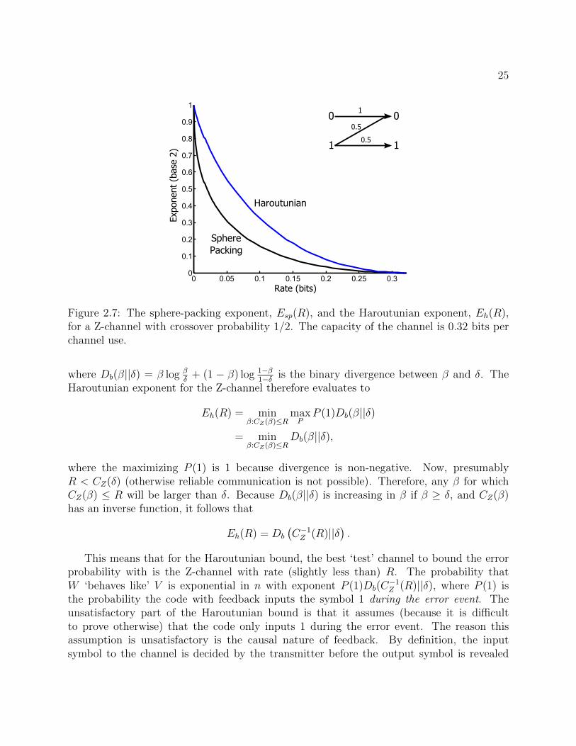
Figure 2.7: The sphere-packing exponent, Esp(R), and the Haroutunian exponent, Eh(R),for a Z-channel with crossover probability 1/2. The capacity of the channel is 0.32 bits perchannel use.

where Db(β||δ) = β log βδ

+ (1 − β) log 1−β1−δ is the binary divergence between β and δ. The

Haroutunian exponent for the Z-channel therefore evaluates to

Eh(R) = minβ:CZ(β)≤R

maxP

P (1)Db(β||δ)

= minβ:CZ(β)≤R

Db(β||δ),

where the maximizing P (1) is 1 because divergence is non-negative. Now, presumablyR < CZ(δ) (otherwise reliable communication is not possible). Therefore, any β for whichCZ(β) ≤ R will be larger than δ. Because Db(β||δ) is increasing in β if β ≥ δ, and CZ(β)has an inverse function, it follows that

Eh(R) = Db

(C−1Z (R)||δ

).

This means that for the Haroutunian bound, the best ‘test’ channel to bound the errorprobability with is the Z-channel with rate (slightly less than) R. The probability thatW ‘behaves like’ V is exponential in n with exponent P (1)Db(C

−1Z (R)||δ), where P (1) is

the probability the code with feedback inputs the symbol 1 during the error event. Theunsatisfactory part of the Haroutunian bound is that it assumes (because it is difficultto prove otherwise) that the code only inputs 1 during the error event. The reason thisassumption is unsatisfactory is the causal nature of feedback. By definition, the inputsymbol to the channel is decided by the transmitter before the output symbol is revealed

26

0 0.05 0.1 0.15 0.2 0.25 0.31

1.2

1.4

1.6

1.8

2

2.2

2.4

1

0.5

1

0 0

0.5

1

HaroutunianSphere Packing

Rate (bits)

Rat

io o

f ex

pone

nts

Figure 2.8: The ratio of the Haroutunian exponent to the sphere-packing exponent,Eh(R)/Esp(R), for a Z-channel with crossover probability 1/2. The ratio tends to a valuegreater than 2 as the rate approaches capacity.

to the receiver and fed back to the transmitter. It stands to reason, therefore, that thetransmitter does not know that the error event will definitely occur until at least partwaythrough the block because there are output sequences that lead to error as well as thosethat do not, which share the same common initial sequence. By memorylessness of thechannel and causality of feedback, the transmitter cannot only input the symbol 1 without‘abandoning’ those output sequences that do not lead to error.

Figure 2.7 plots the sphere-packing and Haroutunian exponents for a Z-channel withcrossover probability 1/2. They are equal at rates 0 and C(W ) but there is a sizable gap forall rates in between. Figure 2.8 shows the ratio of the two exponents. Interestingly, the ratioof the exponents is always larger than 2 (for the Z-channel) as the rate approaches capacity.

2.1.3 An alternate view of the rate-reliability tradeoff

The reliability function characterizes the relationship between rate, blocklength and errorprobability for optimal codes by fixing a rate and blocklength and asking the (approximate)error probability of the optimal code of that rate and blocklength. This error probabilityturns out to be exponential in blocklength, so one can invert this relationship to get boundson the required blocklength to achieve a given rate and desired error probability. There isan alternate view of the tradeoff between these fundamental performance parameters. Thisview looks at the maximum achievable rate for a given blocklength n, and allowable error

27

probability ε. For block codes without feedback, let this quantity be defined as

R∗(n, ε),

while the same quantity for block codes with feedback is denoted R∗f (n, ε). We know fromthe channel coding theorem and converse (with feedback), that for a DMC W ,

limn→∞

R∗(n, ε) = limn→∞

R∗f (n, ε) = C(W ).

Polyanskiy, et. al. [29] have built on prior work and shown that

R∗(n, ε) = C(W )−√σ2W

nQ−1(ε) +O

(log n

n

),

where σ2W is a channel dependent constant called the channel dispersion andQ−1 is the inverse

of the standard Gaussian Q function. This view of the rate-reliability tradeoff is derived fromthe central-limit theorem perspective of the limiting distribution for mutual information, asopposed to the large-deviations perspective that gives rise to error exponents. For symmetricchannels, they have also shown that [11]

R∗f (n, ε) = C(W )−√σ2W

nQ−1(ε) +O

(log n

n

)(2.8)

even though feedback is available. Therefore, for symmetric channels, feedback does notsignificantly improve the rate-reliability tradeoff from this perspective either. As notedin [11], this should not be surprising because the sphere-packing exponent is the governingerror exponent for block codes with and without feedback. Further, the behavior of thesphere-packing exponent around capacity is given by

Esp(R) ' (C(W )−R)2

2σ2W

,

a fact possibly due to moment generating functions being at the heart of proofs of boththe central-limit theorem and large-deviations theorems. Unfortunately, it is not known iffor asymmetric channels like the Z-channel, whether the approximation of (2.8) still holds,leaving the door open for an improvement in the rate-reliability tradeoff from this perspectivewith feedback for asymmetric channels. Again, this may incidentally be due to the fact thatthe Haroutunian bound has significantly different behavior around capacity than the sphere-packing bound, as seen in Fig. 3.3. The hope is that if one can even prove an upper bound toEfb(R) that has the same behavior around capacity as Esp(R), then feedback can be shownto be useless for improving rate for a fixed reliability over asymmetric channels from thisalternative point of view.

28

2.1.4 Contributions

Unfortunately, we have not been able to show that the sphere-packing bound holds withfeedback (i.e., Efb(R) ≤ Esp(R)) for general DMCs. The main contribution of this chapteris a documentation of the progress made in our understanding of this difficult problem. Thisprogress was made both by succeeding in proving partial results towards sphere-packing inspecial cases as well as by failing to get to there in general through what looked to be severalpromising methods. A minor contribution is a description of why the proof in a paper bySheverdyaev [30] claiming that Efb(R) ≤ Esp(R) for general DMCs has serious flaws, whichcan be read in Appendix A.7.

First, the failures (presented in Section 2.4) are described. Upon seeing Haroutunian’sexponent and its change-of-measure approach to error exponents, the first exploratory at-tempt at the problem might be to try Fano’s inequality. At first glance, the restriction oncapacity in (2.6) is useful because we know that if the capacity of V is too small, the errorprobability will be bounded away from 0. We do not require the capacity of V to be toosmall to reach this conclusion however. By Fano’s inequality, we need only that the mutualinformation across the channel is too low. If PV is the input distribution for a given codewith feedback when11 the channel is V and I(PV , V ) ≤ R − ε (for some small ε > 0), theerror probability under channel V is bounded away from 0 (even if the capacity of V is largerthan the rate). The exponent of the error probability for a given code can then be shown tobe upper bounded by

minV :I(PV ,V )≤R−ε

D(V ||W |PI,V ), (2.9)

where PI,V is the distribution of the input restricted to the error causing output sequencesfor each message. Through our interactions with Baris Nakiboglu at MIT, we knew that(somewhat surprisingly)

minV :I(PV ,V )≤R−ε

D(V ||W |PV ) ≤ Esp(R− ε), (2.10)

but such a conclusion is difficult to reach in (2.9) because nothing is known about PI,V . Forexample, without more information, PI,V could place all its mass on the x that maximizesD(V (·|x)||W (·|x)) for each V . Further, without more information, the only V for which wedefinitively know that I(PV , V ) ≤ R − ε are those V for which C(V ) ≤ R − ε. So withoutinformation to refute these last two points, the exponent of (2.9) reduces to

minV :I(PV ,V )≤R−ε

D(V ||W |PI,V ) ≤ minV :C(V )≤R−ε

maxx

D(V (·|x)||W (·|x))

= Eh(R− ε),11If the code has feedback, the input distribution depends on the probability measure on the output

sequences, which in turn depends on the channel.

29

which is of course the Haroutunian exponent.At this point, one might think that in order to make use of (2.10), we should try to show

that PI,V ' PV . One way of showing that PI,V ' PV is to show that under channel V , theerror probability is very close to 1. If C(V ) ≤ R − ε, this conclusion is called the strongconverse, but we want to show that the error probability is close to 1 even if I(PV , V ) ≤ R−ε.This conclusion actually turns out to be untrue, and we give a basic counterexample showingthat this kind of ‘refined’ strong converse does not hold.

Following this development, we stepped back and thought about what makes codes withfeedback different from codes without feedback. The only reason that codes with feedbackcould conceivably beat the sphere-packing bound is that they might learn that the channelis behaving atypically and change their input distribution accordingly. Causality of feedbackand memorylessness of the channel should imply that the Haroutunian bound is unattainable,but perhaps doing better than sphere-packing is not out of the question. The last failureattempted to combat this reasoning by allowing the test channel V to also adapt accordingto the strategy of the code. Essentially, we let the test channel have memory, i.e., at eachtime, the test channel depends on the output sequence received so far. For each time instantin the block and received sequence at that time, the received channel is chosen optimally(i.e., the sphere-packing test channel) depending on the posterior input distribution. Due tosome technical difficulties we had with convergence of random variables, we were not ableto show that this choice of test channel yields the sphere-packing bound, but we conjecturethat it does.

Finally, we worked backwards. We assumed that the sphere-packing bound holds withfeedback and attempted to reduce this fact to a simple condition on codes with feedback andtheir encoding trees. This approach does not appear to be very illuminating, but providesan alternative statement to aim to prove, and is described in Section 2.6.

In terms of partial results, our first one came out of bridging from codes without feedbackto codes with feedback. The natural candidate for a code that uses feedback but does notchange its “strategy” during the block is a code composed of what we term ‘fixed-typeencoding trees’. In a fixed-type encoding tree (an encoding tree is the encoding functionfor one message in a code), the type (or composition or empirical distribution) of the inputsequence is the same for every received sequence. This restriction does not preclude the codefrom using the feedback in a non-trivial way. We show that in this special case, the codeappears to not be using feedback at all. What is meant by this is that, for any conditionaltype that relates input sequences to output sequences, the number of output sequenceswith that conditional type is exactly the same as when the code does not have feedback(but instead uses a codeword of the same input type). This can be used to prove that thesphere-packing bound holds by the usual combinatorial approach. What is interesting aboutthis result is not that the sphere-packing bound continues to hold (which can be shown bychange-of-measure and Fano’s inequality), it is that the sizes of the conditional shells areexactly the same as they would be if the code did not use feedback. This insight is describedin Section 2.5.

30

The second partial result moves in the direction of making the feedback model morerealistic. When proving upper bounds to Efb(R), we assume that the feedback is noiselessand delay-free, as this is the best that one could hope for in practice. In reality, however,for the same reasons that noise and delay impair the forward channel W , they also impairthe output feedback. Our partial result in Section 2.7 shows that if the output feedback isdelayed by T symbols, the error exponent is upper bounded by

Efb,T (R) ≤ Esp

(R−O

(log T

T

))+O

(log T

T

). (2.11)

In the limit as T tends to infinity, we see that the sphere-packing bound must hold. Thisresult shows that feedback information about the very far past is useless for improving theerror exponent. It also complements recent results of Baris Nakiboglu and Giacomo Como(which are commented on in Section 2.9), who showed that the sphere-packing bound holdsfor codes with feedback if the encoders are restricted to hold information about the verynear past only.

The result of (2.11) naturally leads into the question of what the Haroutunian exponentbehaves like for parallel channels. The reason is that, instead of thinking of using the channelW one symbol at time with a delay of T symbols in the feedback path, we can think of usingW T symbols at a time with a delay of 1 supersymbol (a block of T symbols from Y), witheach use of W being independent of the others. If we let W (T ) denote this T -wise parallelchannel, we show in Section 2.8 that

Eh(TR;W (T )) ≤ TEsp

(R− |X |

Tlog(T + 1);W

),

where the left hand side denotes the Haroutunian exponent for the parallel channel at rateTR and the right hand side denotes T times the sphere-packing exponent for W evaluatedat rate R − O((log T )/T ). Thus, in the limit as T gets large, the normalized Haroutunianexponent for the parallel channel approaches the sphere-packing exponent of W . This is arather surprising discovery when compared to the analogous statements about capacity andsphere-packing exponents for the parallel channel. Namely, the capacity of W (T ) is TC(W )and the sphere-packing exponent of W (T ) at rate TR is TEsp(R;W ). As described in Section2.8, the parallel channel W (T ) starts to look more and more symmetric as T gets large. Whilethis development is not of further use for block coding with feedback, it is used in Chapter3 to show that the Haroutunian exponent can be tightened to sphere-packing for fixed delaycodes.

To conclude the chapter, we discuss the current state of affairs for the error exponentwith feedback for general DMCs. As a final introductory remark, we note that much of thework in this chapter came out of discussions with Baris Nakiboglu and Giacomo Como atMIT on the paper of Sheverdyaev [30]. We use two results of theirs in this chapter and citethem accordingly. The result on delayed feedback appears in [31].

31

2.2 Definitions and notation

For those familiar with channel coding in information theory, the notation used in this sectionis introduced in Tables 2.1 and 2.2. For a further description of notation, please see AppendixA.1.

2.3 The sphere-packing and Haroutunian bounds

To understand the motivation for our failed approaches to proving that Efb(R) ≤ Esp(R),it is important to know how the sphere-packing bound is proved for codes without feedbackand how the Haroutunian bound is proved for codes with feedback. We should mention herethat much of the work in this thesis uses the method of types [32] to prove and get intuitionabout discrete, memoryless systems. Knowledge of the method of types will make it mucheasier to understand the material.

Theorem 1 (Sphere-packing for block codes without feedback). Fix a δ > 0. There is afinite nSP (W, δ) such that for n ≥ nSP (W, δ), any block code of length n and rate R withoutfeedback has

− 1

nlogPe(W ) ≤ Esp(R− δ) + δ.

Proof: There are two conceptually different proofs that we will consider. The first isa combinatorial proof by the method of types and the second is a proof motivated by thestrong converse and involves the use of a ‘change-of-measure’. In both proofs, however, a‘pre-processing’ step must be performed. Given any code without feedback of blocklengthn, there is a subcode whose codewords are all of the same type and the rate of this subcodeis at least R− |X |

nlog(n+ 1). So fix this subcode and the common type of its codewords P .

We give here an outline of the two proofs.

• Method of types For a full proof, see Appendix A.2. Given P , we choose the V ∈Vn(P ) that is ‘closest’ to the sphere-packing optimizer, that is

V ∈ arg minU∈Vn(P ):I(P,V )≤R−2δ

D(U ||W |P ).

Consider the V -shells around each xn(m),m ∈ M. These V -shells have cardinality atleast exp(nH(V |P ))/(n+ 1)|X ||Y|, and for every m ∈M, TV (xn(m)) ⊂ TPV , with

|TPV | ≤ exp(nH(PV )) exp

(n

(R− |X |

nlog(n+ 1) +H(V |P )

))because we chose V so that I(P, V ) ≤ R − 2δ and we can assume for large enough n,|X |n

log(n + 1) ≤ δ. Therefore, there must be significant overlap in the V -shells around

32

Notation Descriptionlog, exp Logarithm and exponential to the base e unless otherwise specifiedX Finite channel input alphabetY Finite channel output alphabetW ‘True’ channelV ‘Test’ channelκV maxx,y:V (y|x)>0− log V (y|x)τV minx,y V (y|x)W Set of channel transition matrices with input/output alphabets X and YP Set of distributions on XQ Set of distributions on YPn Set of types of length n for alphabet XVn(P ) Set of conditional types of length n for input type PQn Set of types of length n for alphabet Yxn Vector notation for xn = (x1, . . . , xn) (non-random)Xn Vector notation for Xn = (X1, . . . , Xn) (capital letters for random variables)TP Type class of vectors with type P for some P ∈ Pn

TV (xn) Conditional V -shell of vector xn

H(P ) Entropy of distribution PH(V |P ) Conditional entropy of output of channel V when input has distribution PPV Distribution on Y when input distribution is P and channel is V

(P, V ) Joint distribution in X × Y when input distribution is P and channel is VI(P, V ) Mutual information between input and output of channel V

when input has distribution PI(X;Y ) Mutual information between random variables X and YC(V ) Capacity of channel V

D(P ||P ) Divergence between distributions P and PD(V ||W |P ) Conditional divergence between V and W when input distribution is P||P − P ′||1 L1 distance between P and P ′

hb(δ) Binary entropy −δ log δ − (1− δ) log(1− δ)Db(δ||β) Binary divergence between δ and βEh(R) Haroutunian exponent at rate REsp(R) Sphere-packing exponent at rate R

Table 2.1: Definitions for distributions, channels, types and functions of distributions.

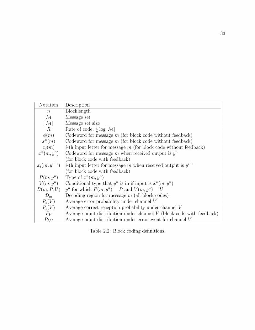
33

Notation Descriptionn BlocklengthM Message set|M| Message set sizeR Rate of code, 1

nlog |M|

φ(m) Codeword for message m (for block code without feedback)xn(m) Codeword for message m (for block code without feedback)xi(m) i-th input letter for message m (for block code without feedback)

xn(m, yn) Codeword for message m when received output is yn

(for block code with feedback)xi(m, y

i−1) i-th input letter for message m when received output is yi−1

(for block code with feedback)P (m, yn) Type of xn(m, yn)V (m, yn) Conditional type that yn is in if input is xn(m, yn)B(m,P, U) yn for which P (m, yn) = P and V (m, yn) = UDm Decoding region for message m (all block codes)Pe(V ) Average error probability under channel VPc(V ) Average correct reception probability under channel VPV Average input distribution under channel V (block code with feedback)PI,V Average input distribution under error event for channel V

Table 2.2: Block coding definitions.

34

each of the messages. The overlap implies that when those sequences lying in overlappingV -shells are output, an error occurs with high probability because each sequence canonly be decoded to one message. For each message, the probability of the output beingin the V -shell around its codeword is approximately exp(−nD(V ||W |P )). The exponentof the error probability is thus approximately

minV ∈Vn(P ):I(P,V )≤R−2δ

D(V ||W |P ).

The set of conditional types for P , Vn(P ), gets ‘close’ to all of W as n gets large, so forlarge n,

minV ∈Vn(P ):I(P,V )≤R−2δ

D(V ||W |P ) ' minV ∈W:I(P,V )≤R−2δ

D(V ||W |P )

, Esp(R− 2δ, P ).

Because Esp(R) = maxP Esp(R,P ), the proof is complete.

• Change of measure For a full proof, see Appendix A.3. Given P ∈ Pn, directly choosethe sphere-packing optimizing V . That is, let

V ∈ arg minU∈W:I(P,U)≤R−2δ

D(V ||W |P ).

Because all the codewords are of type P , and I(P, V ) ≤ R − 2δ, one can prove astrong converse for this subcode12 and show that if n is large, Pe(V ) ' 1. We wantto show that Pe(W ) is lower bounded by the sphere-packing bound, so we perform achange of measure from V to W . The change of measure says that, approximately upto subexponential terms,

Pe(W )

Pe(V )≥ exp (−nD(V ||W |P ))

= exp(−nEsp(R− 2δ, P ))

≥ exp(−nEsp(R− 2δ)).

Because Pe(V ) ' 1, we get that the sphere-packing bound holds.

Now, moving to codes with feedback, the type of the input over the blocklength dependson both the message and the output sequence. The first idea for extending the sphere-packing proofs to codes with feedback might be to group message and output sequence pairs(m, yn) according to the type of the input sequence P (m, yn), and concentrate on the Pwith the largest representation. Unfortunately, there is no guarantee that if we look at

12The usual strong converse says that if C(V ) < R, Pe(V ) tends to 1 as n→∞.

35

a sphere-packing optimizing V and its conditional shell B(m,P, V ) around each message,|B(m,P, V )| is large enough to cause errors with high probability. This is the impedimentthat prevented the original proof of the sphere-packing bound from going through for codeswith feedback, as noted by Shannon, Gallager and Berlekamp [18]. Therefore, Haroutunianlooks at channels V that he knows will cause errors: those that have a capacity lower thanthe rate.

Theorem 2 (Haroutunian bound for block codes with feedback). For any δ > 0, thereexists a finite nh(W,R, δ) such that any fixed-length code with feedback of rate R and lengthn ≥ nh(W,R, δ) has

− 1

nlogPe(W ) ≤ Eh(R− δ) + δ.

Proof: For a full proof, see Appendix A.4. This proof also proceeds by a strong converseand then a change of measure. Fix the Haroutunian optimizing V ,

V ∈ arg minU∈W:C(U)≤R−δ

maxP∈P

D(U ||W |P )

.

Because C(V ) ≤ R − δ, the strong converse with feedback says that Pe(V ) ' 1. A changeof measure shows that, up to subexponential terms,

Pe(W )

Pe(V )≥ exp(−nD(V ||W |PI,V )),

where PI,V is the distribution of the input ‘during the error event’. This distribution could beanything, so to get a bound for all codes, we take the maximum over PI,V to get Haroutunian’sexponent.

2.4 Failed Approaches to proving the sphere-packing

bound for codes with feedback

After being interested in the reliability function with feedback problem for some time, wewere made aware by Baris Nakiboglu at MIT of a paper by Sheverdyaev [30] that claimedto prove that Efb(R) ≤ Esp(R) for all DMCs that have no 0’s. After examining the paper,we found two major flaws (which are described in more detail in Appendix A.7). One flawwas a claim (without proof and stated to be obvious) that

infV :I(PV ,V )≤R

D(V ||W |PV ) ≤ maxP

minV :I(P,V )≤R

D(V ||W |P ) (2.12)

= Esp(R), (2.13)

36

where PV is the average input distribution of a given code when the channel is V . It is not atall obvious how to show (2.12) is true (or whether it is true at all). The problem is the lackof information available about the distribution PV as a function of V . In particular, what ifPV is the capacity achieving distribution for V with C(V ) > R and is a point mass on theHaroutunian exponent maximizing x for V with C(V ) ≤ R? The left hand side of (2.12)would then evaluate to Eh(R). Of course, such a PV is not possible because we know that theinput distribution must be continuous as a function of the channel. Using this information,Nakiboglu [33] was able to prove the following lemma.

Lemma 1. Let PV be any continuous function from W to P, and let for any V ∈ W,κV = maxx,y:V (y|x)>0 log(1/V (y|x)). Then, for all R > 0, ε ≥ 0,

infV :I(PV ,V )≤R

D(V ||W |PV ) + εmax κV , κW ≤ Esp(R) + ε(κW + log |Y|).

The proof of the lemma can be found in Appendix A.5 as it is not available in theliterature and Nakiboglu currently has no plans to publish it. The proof involves consideringa special family of parametrized test channels and using the intermediate value theorem.The fact that maxκW , κV ≤ κW + log |Y| for this family of channels is useful in boundingfor change of measure.

Lemma 1 closes one gap in the proof of Sheverdyaev, but there is a second flaw in thepaper involving Taylor expansions (as detailed in Appendix A.7). This flaw can be exposedby showing that a claim derived by Sheverdyaev (after taking Taylor expansions and using‘uniformly bounded’ constants for the error terms in the expansion) can be refuted by acounterexample. It is our feeling that one philosophical reason why the Sheverdyaev proofdoes not work is because it does not use causality of feedback in a serious way. We believe thatany proof of sphere-packing with feedback must crucially use causality and memorylessnessof the channel.

Imre Csiszar informed us at ISIT 2010 that it was known within the community ofresearchers interested in this problem that there are flaws in the proof of [30]. He alsopointed us to a manuscript of Augustin [34] that was never published in a peer-reviewedformat which claims13 to show that Efb(R) ≤ Esp(R) for all channels. We cannot makea definitive statement about the correctness of Augustin’s proof because of the quality ofthe translation (from German) as well as lack of detail in the proof. See Appendix A.8 forfurther comments.

We now give three of our attempts to prove Efb(R) ≤ Esp(R) for general DMCs, startingwith the simplest idea of using Fano’s inequality to induce errors.

13Csiszar noted that he had never reviewed the proof due to the length of the manuscript and did notknow if it was correct.

37

2.4.1 A first attempt via Fano’s inequality

For any V ∈ W , and a given block code with feedback, let the input distribution underchannel V be

∀ x ∈ X , PV (x) =1

|M|∑m∈M

∑yn

PV (Y n = yn|M = m)1

n

n∑i=1

1(xi(m, yi−1) = x) (2.14)

and let the incorrect input distribution under channel V be

∀ x ∈ X , PI,V (x) =1

|M|∑m∈M

∑yn /∈Dm

PV (Y n = yn|M = m)

Pe(V )

1

n

n∑i=1

1(xi(m, yi−1) = x). (2.15)

To recap, we have just defined two input distributions of the code with feedback asa function of the channel V it faces. The reason new definitions are required is becausethe input distribution of a code with feedback critically depends on the channel behavior.The input distribution of the code can be used to select a channel that we know (by Fano’sinequality) will induce errors because the mutual information of the input distribution (underV ) over channel V is too low. When, we change the measure from V to W , we will see thatthe input distribution that shows up in the divergence is the incorrect input distribution.

Lemma 2 (Not quite sphere-packing via Fano’s inequality). Fix an R > 0 and δ ∈ (1/n,R).For any block code with feedback of rate R and length n,

− 1

nlogPe(W ) ≤ inf

V :I(PV ,V )≤R−δD(V ||W |PI,V ) +

2 maxκV , κW1R

(δ − 1

n

) β(n, |X |, |Y|)+

1

nlog

(1

R

(δ − 1

n

)),

where

β(n, |X |, |Y|) = infε>0

ε+ (n+ 1)|X ||Y| exp

(−nε

2

2

)= O

(√|X ||Y| log n

n

).

This lemma is proved by using Fano’s inequality for channel V and then performing achange of measure from V to W . The full proof is in Appendix A.6.1. The important termabove (that does not decay to 0 as n→∞) is the divergence term.

2.4.2 A refined strong converse

It looks as though the approach given by Fano’s inequality will not yield the sphere-packingbound because we do not know enough about PI,V as a function of V . In fact, the best we

38

can say without further information is that PI,V might be a point mass for a given V (itcannot simultaneously be a point mass that changes for each V because it must at least becontinuous). Therefore, we cannot apply Lemma 1 to get a relation between the exponentin Lemma 2 and the sphere-packing exponent. Seeing this, we posit a property of codeswith feedback that, if it held, would ensure that the sphere-packing bound would hold.Unfortunately, we will show that the condition we posited does not hold and altering it toone that likely does hold would not allow us to prove that the sphere-packing holds.

Definition 1. We say the refined strong converse holds for block codes with feedback if∀δ > 0, V ∈ W , n ≥ 1, there exists a function γRSC(n, δ, R, κV ) such that for any length nblock code with feedback of rate R, if I(PV , V ) ≤ R− δ, then

Pc(V ) ≤ γRSC(n, δ, R, κV )

and if δ, R, V are fixed,

limn→∞

γRSC(n, δ, R, κV )→ 0.

This is called the refined strong converse because the standard strong converse requires thatthe probability of error goes to 1 if C(V ) < R, while this refined condition requires onlythat I(PV , V ) < R, where PV is the average input distribution under channel V . Also, werequire that the dependence on V be through κV (and |X | and |Y|, which are suppressed inthe notation), with a smaller κV leading to a smaller upper bound on the error probability.

Lemma 3. If the refined strong converse holds, then for any R > 0, δ ∈ (0, R), thereis a finite nRSC(W,R, δ) such that for any block code with feedback of rate R and lengthn ≥ nRSC(W,R, δ),

− 1

nlogPe(W ) ≤ Esp(R− δ) + δ.

Hence, if the refined strong converse holds, so does the sphere-packing bound.

For the proof of this lemma, see Appendix A.6.2. Essentially, it uses the refined strongconverse assumption to show that if I(PV , V ) ≤ R− δ, ||PI,V − PV ||1 ' 0 and so

infV :I(PV ,V )≤R−δ

D(V ||W |PI,V ) ' infV :I(PV ,V )≤R−δ

D(V ||W |PV ) ≤ Esp(R),

where the inequality is from Lemma 1.While Lemma 3 is correct, the assumption that the refined strong converse holds is not.

In fact, the refined strong converse does not even hold for codes without feedback.

39

Example 1. Consider a binary code without feedback with 1/8 its codewords in the type(1/2, 1/2) and the rest being all zero codewords. So 1/8 of the code can be considered a goodcode, while 7/8 is a bad code that communicates nothing. The average input distribution ofthe code is PV = (15/16, 1/16) for all V ∈ W (where W is the set of binary input, binaryoutput channels). Suppose the rate of this code is R = 1− hb(1/3) ' 0.082 bits per symbol.

Now let V be a binary symmetric channel with crossover probability 1/4, so C(V ) =1 − hb(1/4) ' 0.19 bits per symbol. Now, I(PV , V ) = 0.046 < R = 0.082. However, thesubcode composed of type (1/2, 1/2) codewords can be a very good code and its rate is about0.082 for large n. The channel V has capacity 0.19 > 0.082, so this good subcode can have avery low error probability (say about 0). Hence, the probability of error for large n is upperbounded by approximately 7/8 and does not approach closer to 1 in the limit. Therefore therefined strong converse does not hold.

With this example in mind, what is likely to be true is a weaker refined strong converse,a condition that we define below.

Definition 2. We say the refined strong converse with message selection holds if forn ≥ nMS(R, δ, |X |, |Y|), δ > 0, R > 0, V ∈ W, there is a γMS(n, δ, R, κV ) such that for alllength n, rate R codes with feedback, if I(PV , V ) ≤ R − δ, there is a subcode (a subset of

messages) of rate at least R− |X ||Y|n

log(n+ 1) with

Pc(V ) ≤ γMS(n, δ, R, κV )

and γMS(n, δ, R, κV )→ 0 as n→∞ with the other parameters fixed.

The refined strong converse with message selection certainly holds for codes withoutfeedback. In fact, it is how the sphere-packing bound for codes without feedback is proved.Additionally, intuition suggests that it is also true for codes with feedback. Unfortunately,if we assume that the refined strong converse with message selection holds for codes withfeedback, it does not immediately follow that the sphere-packing bound holds as in Lemma 3.The reason is that Lemma 1 requires that the input distribution PV be continuously varyingwith V . When the strong converse only holds for a subset of messages, it is possible that thesubset can depend on the test channel V . Therefore PV will vary discontinuously with Vif that subset changes (as the subset must change discontinuously with V , being a discreteobject). It is unclear if an additional argument on top of this can be made to somehow‘smooth out’ the discontinuity with V by adding in terms from different messages accordingto how far the messages are from lying in the ‘bad’ subcode guaranteed by Definition 2.

2.4.3 A test channel with memory

As mentioned earlier, another approach we took was to step back and give ourselves a widerchoice of test channels to force errors for a code with feedback. We will do so by allowing

40

the test channel to depend on the received sequence (essentially using a test channel with

memory). For a given block code with feedback, let V denote a probability measure onM×X n × Yn with

PV (m,xn, yn) =1

|M|

n∏i=1

1(xi(m, yi−1) = xi)Vyi−1(yi|xi),

where Vyi ∈ W for i = 0, . . . , n−1, yi ∈ Y i. Let Pyi ∈ P denote the input distribution under

measure V after the channel output yi has been received. That is,

∀ x ∈ X , Pyi(x) =1

|M|∑m∈M

PV (Y i = yi|M = m)

PV (Y i = yi)1(xi+1(m, y

i) = x)

=∑m∈M

PV (M = m|Y i = yi)1(xi+1(m, yi) = x), (2.16)

where

PV (Y i = yi) =1

|M|∑m∈M

PV (Y i = yi|M = m).

Note that the Pyi are defined recursively. That is, first define for y0 = ∅,

P∅(x) =1

|M|∑m∈M

1(xi(m) = x).

Then, set a V∅ ∈ W . The choice of V∅ now induces the measure PV (Y 1 = y1|M = m) foreach m through the code, which in turn induces the input distribution Py1 for each y1 ∈ Y1

through (2.16). Now, for each y1 ∈ Y1, set a Vy1 ∈ W . Thereafter, an input distribution Py2

is induced for each y2 ∈ Y2, and so on. Hence, if just choose Vyi for each yi, i = 0, . . . , n− 1,

the measure V is well defined. The channel Vyi depends on the received sequence yi and

hence the test channel V is a channel with memory. Additionally, like the test channel usedin the proof of the sphere-packing bound, it should depend on the code to give a good lowerbound to the probability of error. This attempt at least tries to use causality of feedback ina nontrivial way in order to prove a lower bound for the error probability. For each time andwith each received sequence, we are attempting to see what happens if the best (in terms ofdivergence), bad (in terms of mutual information) channel shows up.

The intuition for attempting this approach is that a code with feedback can potentiallychange its coding strategy according to how ’good’ or ’bad’ the channel is. Indeed, this isexactly the reason why Haroutunian’s bound contains the maximization over input distribu-tions inside the minimization over channels. However, we know that even though the codecan adaptively change its input, it cannot ‘predict’ whether the channel will be good or bad.

41

At best, it can only react to whether the channel has been good or bad up to the presenttime because of the causal nature of feedback. Therefore, allowing the channel to depend onthe past received symbols might allow us to tailor the error inducing channel to the part ofthe encoding tree we are in. With that in mind, we will make the following choice for Vyi :

Vyi ∈ arg minV ∈W

D(V ||W |Pyi

): I(Pyi , V

)≤ R− 2δ

,∀ i = 0, . . . , n− 1, yi ∈ Y i (2.17)

for some small δ > 0.At this point, we will do two things with this test channel with memory. First, we will

show that if two statements about the code used over this test channel with memory aretrue, then the sphere-packing bound holds. Second, we will consider the technical obstaclesin showing that those two technical statements are true for the choice of V in (2.17).

First, we will show that the sphere-packing bound must hold for channel W providedtwo statements can be made with high probability. This approach is adapted from theinformation-spectrum literature [35].

Lemma 4 (Information Spectrum Converse). Let V be a measure14 on M× Yn. Fix aδ > 0. Let15

A ,

(m, yn) :

1

nlog

PV (Y n = yn|M = m)

PV (Y n = yn)≤ R− δ

(2.18)

B ,

(m, yn) :

1

nlog

PV (Y n = yn|M = m)

PW (Y n = yn|M = m)≤ Esp(R− 2δ) + δ

(2.19)

E , (m, yn) : yn /∈ Dm .

Then,

Pe(W ) ≥ exp (−n [Esp(R− 2δ) + δ])[1− exp(−nδ)− PV (Bc)− PV (Ac)

].

Hence,

Pe(W ) ≥ exp(−n[Esp(R− 2δ) + 2δ])

for large n provided

PV

(1

nlog

PV (Y n|M)

PV (Y n)≤ R− δ

)→ 1, n→∞ (2.20)

PV

(1

nlog

PV (Y n|M)

PW (Y n|M)≤ Esp(R− 2δ) + δ

)→ 1, n→∞. (2.21)

14Of course, this measure is induced from one on M×Xn × Yn.15Recall that capital letters are used to denote random variables while lower case vectors denote nonrandom

realizations.

42

A proof of the lemma can be found in Appendix A.6.3. Our task now would be to showthat with the choice of V in (2.17), statements (2.20) and (2.21) hold. Unfortunately, this

task is harder than in the case when V does not have memory and the code does not havefeedback. First, note that

Z ,1

nlog

PV (Y n|M)

PV (Y n)

=1

n

n∑i=1

logPV (Yi|M,Y i−1)

PV (Yi|Y i−1)

=1

n

n∑i=1

logVY i−1(Yi|Xi(M,Y i−1))∑x PY i−1(x)VY i−1(Yi|x)

=1

n

n∑i=1

Zi

Zi , logPV (Yi|M,Y i−1)

PV (Yi|Y i−1). (2.22)

Similarly,

Z ,1

nlog

PV (Y n|M)

PW (Y n|M)

=1

n

n∑i=1

logPV (Yi|M,Y i−1)

PW (Yi|M,Y i−1)

=1

n

n∑i=1

logVY i−1(Yi|Xi(M,Y i−1))

W (Yi|Xi(M,Y i−1))

=1

n

n∑i=1

Zi

Zi , logPV (Yi|M,Y i−1)

PW (Yi|M,Y i−1). (2.23)

Zini=1 and Zini=1 are random variables whose normalized sums are equal to Z and Zrespectively. Now, we have two claims that amount to nothing more than algebraic book-keeping (the proofs can be found in Appendix A.6.3).

Proposition 1. With the choice of V in (2.17) and the definitions of Zi and Zi in (2.22)

43

and (2.23) respectively, we have for i = 1, . . . , n,

EV [Zi] =∑

yi−1∈Yi−1

PV (yi−1)I(Pyi−1 , Vyi−1) ≤ R− 2δ (2.24)

EV [Zi] =∑

yi−1∈Yi−1

PV (yi−1)Esp(R− 2δ, Pyi−1) ≤ Esp(R− 2δ). (2.25)

Therefore, by linearity of expectation,

EV [Z] ≤ R− 2δ < R− δ

EV[Z]≤ Esp(R− 2δ) < Esp(R− 2δ) + δ.

Proposition 1 shows the rationale behind setting V as in (2.17). The random variables wewant to converge with high probability in (2.20) and (2.21) have expectations on the properside of R − δ and Esp(R − 2δ) + δ respectively at least. Now, this is a good start, but atthis point all standard ways of proving convergence in probability of a normalized sum ofrandom variables fail because of one crucial point. The point is that the expectations in(2.24) and (2.25) are averaged over both M and Y n. Necessarily, any ‘off-the-shelf’ proofof convergence will require the Zi to be independent or weakly dependent in some sense,otherwise convergence does not hold in general. Unfortunately, while that may be the caseif M is held random while Zi is averaged over, it cannot be the case for general codes oncewe fix M = m. That is, the course of 1

n

∑ni=1 Zi strongly depends on M and information

about M may be revealed in Z.For example, consider forming a martingale sequence as follows. Let the filtration be

defined as Fi = σ(M,Y i), and let

Ti ,1

n(Zi − EV [Zi|Fi−1])

T =n∑i=1

Ti.

Then, T is a martingale because the Ti are zero mean martingale differences by construc-tion. So with appropriate boundedness restrictions on Ti, we know that T → 0 with highprobability (w.h.p.). Notably, however, this only implies that

1

n

n∑i=1

Zi →1

n

n∑i=1

EV [Zi|Fi−1] w.h.p.

44

But,

EV [Zi|Fi−1] = EV[Zi|M,Y i−1]

= EV

[log

PV (Yi|M,Y i−1)

PV (Yi|Y i−1)

∣∣∣∣∣M,Y i−1

]

=∑y

PV (Yi = y|M,Y i−1) logPV (Yi = y|M,Y i−1)

PV (Yi = y|Y i−1)

=∑y

VY i−1(y|Xi(M,Y i−1)) logVY i−1(y|Xi(M,Y i−1))

(PY i−1VY i−1)(y)

6= I(PY i−1 , VY i−1

)=∑x

PY i−1(x)∑y

VY i−1(y|x)) logVY i−1(y|x))

(PY i−1VY i−1)(y).

We see that EV [Zi] 6= I(PY i−1 , VY i−1) and therefore, it is difficult to say much about what Zconverges to except that the average of what it converges to over M,Y n is less than R − δ.The same problem arises when we attempt to analyze the convergence of Z.

This argument, of course, does not preclude one from using more information about theZ and Z processes to obtain convergence results in probability. Indeed, it is our opinionthat the event when Z is below R − δ and Z is below Esp(R − 2δ) + δ has non-negligibleprobability for large n.

Conjecture 1. With the choice of V as in (2.17), it is true that for some g(δ) > 0,

PV

(1

nlog

PV (Y n|M)

PV (Y n)> R− δ

)≤ 1

2− g(δ), n→∞

PV

(1

nlog

PV (Y n|M)

PW (Y n|M)> Esp(R− 2δ) + δ

)≤ 1

2− g(δ), n→∞.

Thus, while there may not be true convergence for the two events, there should at leastbe non-negligible overlap of the complementary events.

2.4.4 The back-story bound

One of the unsatisfying elements of the Haroutunian exponent is that it leaves open thepossibility that one should try to design the channel W to be asymmetric in order to beatthe sphere-packing exponent with feedback. However, we know that for output-symmetricchannels, the sphere-packing bounds holds (because Eh(R) = Esp(R) for those channels).This fact suggests a possible strategy to show that Eh(R) is not achievable for some asym-metric channels. The idea is, given a symmetric channel such as a BEC, the decoder can add

45

noise to the output symbols to simulate an asymmetric channel. The upper bound on theerror exponent for the symmetric channel then also is an upper bound for the asymmetricchannel because the contraposition leads to a contradiction.

Suppose that the error exponent for the simulated asymmetric channel is indeed largerthan the error exponent for the symmetric channel. Then we can code over the symmetricchannel by adding noise at the decoder and simulating the asymmetric channel. We thushave a contradiction if the error exponent for the asymmetric channel is larger than the errorexponent for the symmetric channel. We call this the back-story bound. Unfortunately, inthe examples we have tried, the resulting bound is weaker than the Haroutunian bound.Appendix B.2 shows how a Z-channel simulated by a BEC followed by collapsing the erasureand 0 symbols does not give a better bound than the Haroutunian exponent for the Z-channel.

2.5 Sphere-packing holds when the fixed type encoding

tree condition holds

Thus far, we have attempted to show that Efb(R) ≤ Esp(R) by looking at feedback codesat a high level. In Section 2.4.3, we attempted to use memoryless of the channel to choosethe test channel optimally at each time (and received sequence). Calculating bounds on therelevant probabilities turn out to be difficult, however. We turn our attention now to someanalyses that look at codes with feedback in more detail.

In this section, we will show that the sphere-packing bound holds for a restricted class ofcodes with feedback. The restricted class of codes is said to have encoding trees that satisfythe ‘fixed type encoding tree’ condition. In these codes, the input codewords all have thesame type regardless of the received sequence. The fact that sphere-packing holds for thisrestricted class of codes with feedback can be proved analogously to Haroutunian’s boundfor codes without feedback, by first proving a strong converse and then analyzing the errorprobability after a change-of-measure. We will, however, prove it in a combinatorial manner,analogous to Theorem 1. This approach will illuminate a somewhat surprising fact: that ifone is restricted to using a fixed type P (with feedback) for a given message, at the output,it looks as if feedback is not being used at all. The precise meaning of this statement will begiven later.

Definition 3 (Fixed type encoding tree condition). An encoding tree of an arbitrary messagem ∈M for a fixed-length code with feedback is said to satisfy the fixed type encoding treecondition if there exists a P ∈ Pn such that for all yn ∈ Yn, P (m, yn) = P . Recall thatP (m, yn) denotes the type of the input codeword for message m along a received sequence yn,i.e., the type of (x1(m), x2(m, y

1), . . . , xn(m, yn−1)).

Note that an encoding tree satisfying the fixed type encoding tree condition need not giveup the use of feedback. That is, the channel input codeword can still depend non-trivially

46

on the received sequence. For example consider the encoding tree in Figure 2.9. The channelinput codewords along different received sequences are not necessarily the same.

Proposition 2. Suppose an encoding tree for a message m ∈ M satisfies the fixed typeencoding tree condition with type P ∈ Pn. Then, for all V ∈ Vn(P ),

|B(m,P, V )| = |TV (xn)|

≥ exp(nH(V |P ))

(n+ 1)|X ||Y|,

where xn ∈ TP is arbitrary because |TV (xn)| depends only on the type of xn.

This proposition says that if the types of the input vectors are the same for all yn, thenthe conditional V -shells have the same size as for a code without feedback. This may besomewhat surprising, because in some sense, even though the encoding tree can use feedbacknontrivially, it appears at the output (through the conditional relationship between input andoutput) as if feedback had not been used at all. Before proving the proposition rigorously,we give some intuition for why this result might hold. First, note that

B(m,P, V ) = yn : P (m, yn) = P, V (m, yn) = V

=

yn : ∀ x, y,

n∑i=1

1(xi(m, yi−1) = x, yi = y) = nP (x)V (y|x)

=

yn : ∀ x, y,

n∑i=1

1(xi(m, yi−1) = x, yi = y) ≤ nP (x)V (y|x)

.

The last line follows because if

n∑i=1

1(xi(m, yi−1) = x, yi = y) 6= nP (x)V (y|x),

then there is at least one x, y with∑n

i=1 1(xi(m, yi−1) = x, yi = y) > nP (x)V (y|x) because

∑x,y

n∑i=1

1(xi(m, yi−1) = x, yi = y) =

∑x,y

nP (x)V (y|x) = n

and all terms in the sum are non-negative.Consider the encoding tree for a message in a code with feedback as shown in Figure

2.9. We wish to count sequences yn that end up in B(m,P, V ). Since P (m, yn) = P for allyn ∈ Yn, we need to verify that V (m, yn) = V for a given yn to be in B(m,P, V ). Consider

47

Time1 32

0

1

1

1

1

0

0

0

0

0

0

0

0

0

0

1

1

1

1

1

Figure 2.9: A nontrivial encoding tree for a code with feedback, n = 3,X = Y = 0, 1. Asymbol at a node denotes a channel input and a symbol on an edge denotes a channel output.The type of x3(m, y3) is (2/3, 1/3) for all y3 ∈ Y3, so this encoding tree satisfies the fixedtype encoding tree condition. It uses feedback nontrivially, however, as x3(m, (0, 0, 0)) =(0, 0, 1) 6= x3(m, (1, 1, 1)) = (0, 1, 0).

48

marching along a received sequence from left to right in Figure 2.9. If yn /∈ B(m,P, V ),there is some minimal k such that

∀ x, y,k∑i=1

1(xi(m, yi−1) = x, yi = y) ≤ nP (x)V (y|x)

and

∃ x, y such thatk+1∑i=1

1(xi(m, yi−1) = x, yi = y) > nP (x)V (y|x).

In other words, we are marching along yn from left to right and at time 0, y0 = ∅ stillhas children in B(m,P, V ), y1 still has children in B(m,P, V ), . . . , yk still has children inB(m,P, V ), but yk+1 has no children in B(m,P, V ). On the graph of the encoding tree, withnodes corresponding to channel inputs and edges corresponding to channel outputs, we canvisualize this by pruning the tree at the edge corresponding to yk+1. The rule for whetheror not to prune an edge does not change whether a code has feedback or not, and in somesense the pruning of an edge in one part of the tree does not affect any other part of the treethat is not a child. Therefore, one might intuitively deduce that B(m,P, V ) should have atleast the same size as TV (xn) for some xn in TP .

The proposition is proved rigorously (in Appendix A.9.1) by showing that given anyxn ∈ TP , there must exist a one-to-one mapping τ from Yn to Yn that has the followingproperty. For all yn ∈ Yn, if yn ∈ TV (xn) for some V ∈ Vn(P ), then τ(yn) ∈ B(m,P, V ).Therefore, it is not possible via feedback to move sequences into ‘good’ V -shells (thosewith high mutual information) from ‘bad’ ones (those with low mutual information) if thefixed type condition holds. Using Proposition 2, one can prove that the sphere-packingbound holds analogously to the method of types proof of sphere-packing for codes withoutfeedback.

Theorem 3 (Sphere-packing holds if fixed type encoding tree condition holds). Fix a δ >0, R > 0. There exists a finite nFT (W,R, δ) such that for any fixed-length code with feedbackof length n ≥ nFT (W,R, δ) and rate R with encoding trees for all messages satisfying thefixed type encoding tree condition,

− 1

nlogPe(W ) ≤ Esp(R− δ) + δ.

For a proof, see Appendix A.9.2.

2.6 What needs to be proved for sphere-packing to

hold for fixed-length codes with feedback?

This section addresses the question of what is needed to prove the sphere-packing bound forfixed-length block codes with feedback. There are many potential answers to that question,

49

but here we give one take on what sets apart the case with feedback from the case withoutfeedback. To that end, we will define two ‘assertions’. The first assertion, call it A, is thatthe sphere-packing bound holds for codes with feedback. The second assertion, call it B,roughly says that encoding trees for codes with feedback are not so different from inputcodewords for codes without feedback in the way that output sequences are related back tothem.

In this section, we show that if B holds, then so must A. It would be tempting to alsoclaim that if A holds, then so does B, as we would then have an equivalent statement aboutencoding trees that would both imply and be implied by the assertion that sphere-packingholds for codes with feedback. Rather, what we can show holds is a much weaker condition,call it C, on all the encoding trees in an arbitrary code of length n and rate R. We will showthat A implies C and C implies A, and hence B also implies C. All in all, we will have

B ⇒ A⇔ C.

Definition 4 (SP holds with feedback). We say that sphere-packing holds for fixed-lengthcodes with feedback, or SP holds with feedback for short, if for all δ > 0, R > 0 andW ∈ W, there is a finite nSP,fb(δ, R,W ) such that any fixed-length code with feedback of rateat least R and length n ≥ nSP,fb(δ, R,W ) has

− 1

nlogPe(W ) ≤ Esp(R− δ) + δ.

Definition 5 (SP Encoding Tree Condition). We say that the sphere-packing encodingtree condition holds, if for all δ > 0, R > 0,W ∈ W, there is a finite nET,fb(δ, R,W ) suchthat the following is true. Given any encoding tree for a fixed-length code with feedback oflength n ≥ nET,fb(δ, R,W ), there exists a P ∈ Pn, V ∈ Vn(P ) (dependent on the encodingtree) such that

|B(m,P, V )| ≥ exp(n(H(V |P )− δ)) (2.26)

D(V ||W |P ) ≤ Esp(R− 2δ) + 2δ (2.27)

I(P, V ) ≤ R− 2δ, (2.28)

where the m in B(m,P, V ) is an indicator of the encoding tree in a code.

Whether the sphere-packing encoding tree condition is a true assertion is unproven cur-rently. The impetus behind its definition is to look at the proof of the sphere-packing theoremfor block codes without feedback. In both the case with and without feedback, showing theexistence of a P ∈ Pn and channel V with I(P, V ) ≤ R−δ and D(V ||W |P ) ≤ Esp(R−δ)+δis straightforward for large n. In the case without feedback, we have good estimates forthe size of the ‘typical’ output under channel V for a given message with codeword typeP , namely it is exponential in H(V |P ). This allows us to prove the part of the statement

50

Time1 2

1

10

1

0

1

0

1

0

1

0

0

0

0

00

0

00

0

0

0

0

00

0

000

0

00

0

00

1111

3 4 5

(0,0,0,0,0)

(1,0,0,0,0)

(1,1,0,0,0)

(1,1,1,0,0)

(1,1,1,1,0)

(1,1,1,1,1)

Figure 2.10: The encoding tree of Example 2 that inputs X1 = 1 and Xi+1 = Yi for 1 ≤ i ≤ 4,with n = 5. Nodes in the tree represent input symbols, while edges represent channel outputsymbols. Only paths in the tree that occur with non-zero probability when W is a Z-channelare shown.

in (2.26) after selection of a P, V that satisfy (2.27) and (2.28). In the case of codes withfeedback, however, the portion of the statement in (2.26) certainly does not hold for anarbitrary P, V because we do not know much about the types of the input codewords alongdifferent received sequences. We look at a simple example to explore the difficulty in provingthe sphere-packing encoding tree coding in general.

Example 2. Suppose X = Y = 0, 1 and W is a Z-channel with crossover probability 0.5.Consider the encoding tree for which (for arbitrary n),

X1 = 1

Xi+1 = Yi, i ≥ 1.

For this example (the encoding tree is shown in Figure 2.10), there are only n + 1 stringsyn that occur with non-zero probability (because once a 0 is output, the rest of the output

51

symbols will be 0 with probability 1). The strings and their type and conditional types are:

yn xn(m, yn) P (m, yn) V (m, yn) H(V |P )(0, 0, 0, . . . , 0, 0) (1, 0, 0, . . . , 0) (n−1

n, 1n) Z(1) 0

(1, 0, 0, . . . , 0, 0) (1, 1, 0, . . . , 0) (n−2n, 2n) Z(1/2) 2

nhb(1/2)

(1, 1, 0, . . . , 0, 0) (1, 1, 1, . . . , 0) (n−3n, 3n) Z(1/3) 3

nhb(1/3)

......

......

...(1, 1, 1, . . . , 1, 0) (1, 1, 1, . . . , 1) (0, 1) Z(1/n) hb(1/n)(1, 1, 1, . . . , 1, 1) (1, 1, 1, . . . , 1) (0, 1) Z(0) 0

(2.29)

where Z(p) is shorthand for the Z-channel with crossover probability p and hb(p) = −p log p−(1− p) log(1− p) is the binary entropy function.

This is an important example to keep in mind because, for almost every P ∈ Pn (exceptfor P = (1, 0)), there is a yn ∈ Yn such that P (m, yn) = P . Furthermore, for everyP ∈ Pn that occurs, there is exactly one yn with P (m, yn) = P . So, in this example, ifP ∈ Pn, V ∈ Vn(P ) and D(V ||W |P ) < ∞, either |B(m,P, V )| = 0 or |B(m,P, V )| = 1. Itappears in this example as if the sphere-packing encoding tree condition will not hold becausenone of the |B(m,P, V )| are exponential in n. A closer inspection, however, is in order forthe right hand side column above showing H(V |P ) for all B(m,P, V ) that are not empty.The maximum H(V |P ) there is, for a given n,

kn , max2≤m≤n

m

nhb

(1

m

)= max

2≤m≤n

m

n

(1

mlogm+

m− 1

mlog

m

m− 1

)=

1

nmax

2≤m≤n

(logm+ (m− 1) log

m

m− 1

)=

1

nmax

2≤m≤n(m logm− (m− 1) log(m− 1)) .

The function x log x is convex-∪, so the maximum above occurs when m = n and hence,

kn =1

n(n log n− (n− 1) log(n− 1))

= log n− n− 1

nlog(n− 1)

= logn

n− 1+

1

nlog(n− 1)

≤ 1

n− 1+

1

nlog(n− 1).

52

0 0.05 0.1 0.15 0.2 0.25 0.3 0.35 0.40

0.1

0.2

0.3

0.4

0.5

0.6

0.7

0.8

0.9

1

Rate, Mutual Information (bits)

Expo

nent

(ba

se 2

)Sphere-Packing Exponent

Exponent for example B(m,P,V)

1

0.5

1

0 0

0.5

1

Figure 2.11: This plot shows the sphere-packing exponent when W is a Z-channel withcrossover probability 0.5. Also shown is a scatter plot of D(V ||W |P ) versus I(P, V ) for thefirst 150 (P, V ) = (P (m, yn), V (m, yn)) in (2.29) when n = 2, 000. The plot highlights thefact that as n→∞, there are pairs (P, V ) in (2.29) such that the point (I(P, V ), D(V ||W |P ))is arbitrarily close to (0, 0). Therefore, for this encoding tree, there is a (P, V ) that satisfies(2.26), (2.27) and (2.28).

Therefore, kn = O((1/n) log n) and for every δ > 0, for large enough n, H(V |P ) < δ forevery P, V with |B(m,P, V )| = 1. So for a fixed δ > 0 and large enough n, every P, V with|B(m,P, V )| satisfies (2.26). In order to check that there is a P, V such that (2.27) and(2.28) hold as well, we plot I(P, V ) versus D(V ||W |P ) for n = 2, 000 in Figure 2.11. Forthis example encoding tree, for large enough n, there are (P, V ) that are arbitrarily close to(0, 0), so the sphere-packing encoding tree condition holds almost trivially. This correspondsto using the sequences with just a few 1’s at the beginning in order to prove error bounds.

Currently, it seems difficult to prove the sphere-packing encoding tree condition holdsexcept in special cases (like an encoding tree without feedback or one that satisfies the fixedtype encoding tree condition). This example shows the core difficulty. If we fixate on one Pfor which we know that there are sequences with P (m, yn) = P , it is difficult (and untrue)to say that B(m,P, V ) is large for arbitrary V ∈ Vn(P ). All we can say is that there existsat least one V ∈ Vn(P ) for which B(m,P, V ) can be quantified in some way. This V mayhave D(V ||W |P ) > Esp(R) or I(P, V ) > R however and cannot be used to prove the sphere-packing bound. That said, if the sphere-packing encoding tree condition holds (i.e., it can beproved for all codes with feedback), the sphere-packing bound also holds for all codes withfeedback used over general DMCs.

53

Proposition 3 (SP Encoding Tree condition implies SP holds). If the sphere-packing en-coding tree condition holds, then sphere-packing for fixed-length codes with feedback holds.

For a proof of the proposition, see Appendix A.11.1. One might be tempted to say that ifsphere-packing holds for fixed-length codes with feedback, then the sphere-packing encodingtree condition also must hold. Unfortunately, this seems difficult to prove as well. What canbe shown to hold is a much weaker condition.

Definition 6 (Intermediate SP Condition). We say that the intermediate sphere-packingcondition holds, if for all δ > 0, R > 0,W ∈ W, there is a finite nSPI,fb(δ, R,W ) suchthat the following is true. Given any fixed-length code of rate at least R and length n ≥nSPI,fb(δ, R,W ), there exists a P ∈ Pn and V ∈ Vn(P ) such that

D(V ||W |P ) ≤ Esp(R− δ) + 2δ (2.30)

1

nlog

[1

|M|∑m∈M

|B(m,P, V ) ∩ Dcm|

]≥ H(V |P )− [Esp(R− δ) + 2δ −D(V ||W |P )] .

(2.31)

Note that if (2.31) holds, then (2.30) also holds by properties of B(m,P, V ) (Proposition14). However, (2.30) reinforces the intuition that (P, V ) are such that error probabilityunder channel W is at least the probability prescribed by the sphere-packing bound.

The intermediate sphere-packing condition turns out to be equivalent to sphere-packingholding for codes with feedback. For a proof of this result, see Appendix A.11.2. Theintermediate sphere-packing condition is quite un-intuitive, however, so it does not seempromising to attempt to prove that it must hold in general.

Proposition 4 (Equivalence of SP and Intermediate SP condition). If SP holds with feed-back, then the intermediate SP condition holds. Conversely, if the intermediate SP conditionholds, SP holds with feedback.

2.7 Delayed feedback is not useful for very large delays

This section gives an upper bound to the error exponent for block codes used over DMCswith noiseless feedback, where the feedback is delayed by some fixed number of symbols. It isinteresting to consider this problem, because in modern, high rate communication systems,the number of symbols that must be encoded before the encoder receives a previous channeloutput (or more likely, a function of the channel output) can be potentially large. Twopossible reasons for this gap between sending a channel input and receiving informationabout the channel output come to mind: propagation delays and the inherent processingtime for demodulation and other processing at the decoder.

54

Consider communicating 20 symbols per microsecond on a 20 MHz channel over a distanceof 1.5 km (round trip 3km). Even without accounting for processing time, the delay for anelectromagnetic signal to travel to and fro would be 10 microseconds, meaning at least200 symbols should have been transmitted before feedback can be received. Additionally,many communications systems have a half-duplex constraint, meaning they cannot listen andtransmit at the same time. Thus, feedback information may not return until the transmitteris finished transmitting some appropriate ‘block’ of symbols.

Suppose that information about the channel outputs is delayed by T symbols. Then, theresult of this section is that the error exponent for rate R codes used with noiseless feedbackdelayed by T symbols is upper bounded by

Esp(R−O(log T/T )) +O(log T/T ),

where the constants hidden in the big-O notation depend on the channel transition matrixW . Hence, for large delays in the feedback path, the sphere-packing bound is essentiallyan upper bound on the error exponent for fixed-length block codes. To avoid confusion,the result applies to a fixed delay in the feedback path (T ), as the blocklength (n) goes toinfinity. Before giving the result, some definitions germane to this section are in order.

2.7.1 Problem Setup

A rate R, blocklength n coding system is an encoder-decoder pair (E ,D).

Definition 7 (Type 1 Encoder - Delay T feedback). A rate R, blocklength n encoder E usedwith feedback delayed by T symbols is a sequence of maps φini=1, with for 1 ≤ i ≤ T ,

φi : 1, 2, . . . , 2nR → X ,

and for i > T ,

φi : 1, 2, . . . , 2nR × Y i−T → X .

Note that T = 1 is the usual perfect-feedback setting where the encoder is aware of the channeloutput immediately before the next channel input must be selected.

Definition 8 (Type 2 Encoder - T block feedback). This is a more powerful class of encodingsystems than the ‘Delay T feedback’ encoders. Here feedback is provided to the encoder inblocks of T symbols at a time. That is, (Y1, . . . , YT ) is given to the encoder before the encoderchooses XT+1 and in general, the received symbol block (YiT+1, . . . , Y(i+1)T ) is provided to theencoder at time (i + 1)T before the encoder must choose X(i+1)T+1. Hence a blocklength ntype 2 encoder with rate R is a sequence of maps φini=1,

φi : 1, . . . , 2nR × Yb(i−1)/T cT → X .

Note that a type 1 encoder is a restricted type 2 encoder that does not use all possible symbolsthat have been fed back.

55

M WX Y

Delay T

Enc Dec

Figure 2.12: Block coding for a DMC W with delayed feedback.

A blocklength n decoder D is a map

ψ : Yn → 1, 2, . . . , 2nR.

The decoding regions for each message are then Dm , ψ−1(m) = yn : ψ(yn) = m form ∈ 1, . . . , 2nR. The average probability of error for a rate R, blocklength n codingsystem (E ,D) is thus defined as

Pe(n, E ,D) =1

2nR

2nR∑m=1

P(ψ(Y n) 6= m|M = m).

If we let C(n,R, T ) be the appropriate set of blocklength n coding systems with rate atleast equal to R used with delay T feedback type 2 encoders, we define the relevant errorexponent at rate R to be

E(R, T ) = lim supn→∞

− 1

nlog min

(E,D)∈C(n,R,T )Pe(n, E ,D).

Haroutunian’s bound applies to codes without any delay in the feedback path, so it alsoapplies for any T > 1, hence for all T ≥ 1, E(R, T ) ≤ Eh(R).

2.7.2 Error exponent bound for delayed feedback

We prove a bound on type 2 encoding systems, which immediately becomes a bound on type1 encoders as well. Without loss of generality, we restrict attention to n that are multiplesof T , that is n = NT for some N ≥ 1 (i.e., there are N total blocks of size T symbols each).

Lemma 5. Define a channel independent constant

α(T ) ,|X |(2 + |Y|) log(T + 1)

T.

56

Fix an ε > α(T ). Then, for any blocklength n = NT (with N ≥ 1) rate R coding systemwith a type 2 encoder,

− 1

NTlogPe(NT, E ,D) ≤ Esp,T (R− ε) + α(T ) + γ(N, T, ε),

where

Esp,T (R) , maxP∈PT

minV ∈VT (P ):I(P,V )≤R

D(V ||W |P ), (2.32)

and

γ(N, T, ε) =1

NTlog

1

1− exp(−NT (ε− α(T ))).

The proof of this lemma is given in Appendix A.12.1. The proof chooses the test channelV within each block of length T according to the most used type of the input during thatblock. Notice how in (2.32), we have already interchanged the order of the max and minin the Haroutunian exponent, but the set of V is restricted to have low mutual informationover length T . We now give an inequality relating the ‘sphere-packing bound for length-T ’with the sphere-packing bound (proved in Appendix A.12.2).

Lemma 6. For any T ≥ 2|X ||Y|, for all P ∈ PT ,

minU∈VT (P ):I(P,U)≤R

D(U ||W |P ) ≤ Esp

(R− 2|X ||Y| log T

T, P

)+κW |X ||Y|

T+

|X ||Y| log(T/|X |)T

,

where16

Esp(R,P ) , minV :I(P,V )≤R

D(V ||W |P ),

κW , maxx,y:W (y|x)>0

log1

W (y|x).

Putting the two lemmas together, we get

16The constant κW can be arbitrarily large, but is finite for a given W. It is our opinion that the appearanceof κW in our bound is an artifact of the proof method, and not intrinsic to the problem. However, to ourknowledge, such a term appears in most, if not all, proofs of the sphere-packing bound where an explicitlower bound to probability of error as a function of blocklength is given. For example, see Theorem 5.8.1of [17] or Theorem 1 and 2 of [36].

57

0 0.05 0.1 0.15 0.2 0.25 0.30

0.1

0.2

0.3

0.4

0.5

0.6

0.7

0.8

0.9

10 0

1 1

0.5

0.5

Rate (bits)

Expo

nent

T = 5,000

Haroutunian

Sphere Packing

Figure 2.13: A plot of the bound on E(R, T ) from Theorem 4 for the Z-channel with T =5, 000 (all quantities are base 2). The bound is only approaching the usefulness of theHaroutunian bound (which works for all T ≥ 1) at this point.

Theorem 4. For any T ≥ 2|X ||Y|,

E(R, T ) ≤ Esp

(R− α(T )− 2|X ||Y|

Tlog T

)+κW |X ||Y|

T+|X ||Y|T

logT

|X |+ α(T ).

In other words, for type 1 and type 2 coding systems with feedback delay T and rate R,

E(R, T ) ≤ Esp(R−O(log T/T )) +O(log T/T ).

Proof: The result of Lemma 5 is monotonic in the rate, so we need only that RN ≥ Rand bound using R. We have just combined the results of the two lemmas together andtaken the limit as N tends to ∞. The only thing that needs to be checked is that the term

1

NTlog

1

1− exp2(−NT (ε− α(T )))(2.33)

converges to 0 as N →∞ for any ε > α(T ), which is readily seen. Therefore, we can take εarbitrarily close to α(T ) and since Esp is continuous for all R expect possibly the R at whichEsp becomes infinite, we substitute α(T ) for ε.

Figures 2.13 and 2.14 show the resulting bound on E(R, T ) for the Z-channel whenT = 5, 000 and 50, 000 respectively. As can be seen, even at T = 5, 000, the constants in thebound for E(R, T ) do not bring it close enough to Esp to be much more useful than Eh(R),so this problem is not necessarily ‘practically’ solved either.

58

0 0.05 0.1 0.15 0.2 0.25 0.30

0.1

0.2

0.3

0.4

0.5

0.6

0.7

0.8

0.9

10 0

1 1

0.5

0.5

Rate (bits)

Expo

nent

T = 50,000

Haroutunian

Sphere Packing

Figure 2.14: A plot of the bound on E(R, T ) from Theorem 4 for the Z-channel with T =50, 000 (all quantities are base 2). At this point, the upper bound is ‘essentially’ the sameas sphere-packing. If a system has a delay in its feedback path this large for the Z-channel,the feedback does not help increase the error exponent for all practical purposes.

59

W(y|x)

W(y|x)

W(y|x)

. . .

x1

x2

xL

y1

y2

yL

. . .

. . .

W (y |x )(L) L L

Figure 2.15: The parallel channel W (L) obtained by using W L times. Each use of Wis independent. The capacity of W (L) is LC(W ) and the scaled sphere-packing exponentEsp(LR;W (L)) for W (L) at rate LR is equal to LEsp(R;W ).

2.8 The Haroutunian exponent for a parallel channel

In this section, we interpret the result of Section 2.7 and arrive at a surprising conclusion. Wewill think of the block-T feedback coding systems of Section 2.7 (where the encoder receivesoutput symbols in blocks of size T ) as having instantaneous feedback when used over aparallel channel. Shifting notation a bit, let L ≥ 1 be an integer. A block-L feedback systemreceives feedback in increments of L symbols at a time, so consider the parallel channel onegets by using L symbols from X at a time, as shown in Figure 2.15. The block-L feedbacksystem can then be viewed as a code with instantaneous feedback used over the DMC W (L)

with input alphabet X L, output alphabet YL and transition probabilities

W (L)(yL|xL) =L∏i=1

W (yi|xi).

It is straightforward to show that C(W (L)) = LC(W ), and with a bit more effort, it can beshown that Esp(LR;W (L)) = LEsp(R;W ) where Esp(LR;W (L)) denotes the sphere-packingexponent for channel W (L) evaluated at rate LR and Esp(R;W ) denotes the sphere-packingexponent for channel W at rate R. Theorem 4 then shows that

Efb(LR;W (L)) ≤ LEsp(R;W ) +O

(log(L+ 1)

L

).

Another upper bound on Efb(LR;W (L)) can be had by applying the Haroutunian boundto the channel W (L), yielding Efb(LR;W (L)) ≤ Eh(LR;W (L)), where Eh(LR;W (L)) is the

60

Haroutunian exponent for W (L) evaluated at rate LR . Considering that C(W (L)) =LC(W ) and Esp(LR;W (L)) = LEsp(R;W ), it wouldn’t be much of a stretch to guess thatEh(LR;W (L)) = LEh(R;W ). If W is an asymmetric channel such as the Z-channel, then

LEh(R;W ) > LEsp(R;W ) + O(

log(L+1)L

)for large enough L. This means that we have the

following interesting dichotomy: either (a) or (b) below must be true.

(a) We have shown that Efb(LR;W (L)) < Eh(LR;W (L)) for some asymmetric channel W (L)

(W (L) is still asymmetric if W is for all L ≥ 1). That is, we have shown a class of channelsfor which the Haroutunian exponent is strictly loose, which would partially confirm ourhypothesis that sphere-packing is a valid upper bound on the error exponent for blockcodes with feedback for asymmetric channels as well.

(b) The Haroutunian exponent for the parallel channel Eh(LR;W (L)) does not decomposelike the sphere-packing exponent and capacity, i.e.,

Eh(LR;W (L)) < LEh(R;W ).

Surprisingly, it turns out that (b) is true17. In the optimizations that characterizeC(W (L)) (maximization over distributions on X L) and Esp(LR;W (L)) (maximization overdistributions on X L and minimizations over channels from X L to YL), it suffices to considerproduct distributions due to the concavity and convexity properties of mutual informa-tion and divergence. This causes the optimizations to decompose into optimizations overL individual symbols, resulting in the multiplicative scaling. In the optimization for theHaroutunian exponent, it turns out that it is not sufficient to consider channels V from X L

to YL that are independent over time, i.e., V (yL|xL) =∏L

i=1 Vi(yi|xi).

Lemma 7. For the parallel channel W (L) with input alphabet X L, output alphabet YL andtransition probabilities

W (L)(yL|xL) =L∏i=1

W (yi|xi),

we have

Eh(LR;W (L)) ≤ LEsp

(R− |X |

Llog(L+ 1);W

).

Thus, in the limit as L→∞ (because Esp is left-continuous),

limL→∞

1

LEh(LR;W (L)) ≤ Esp(R;W ).

17While (a) may be true in the sense that the Haroutunian exponent is strictly loose for some class ofasymmetric channels, we have not shown it to be true by the result in Section 2.7.

61

Note that for all L,

1

LEh(LR;W (L)) ≥ 1

LEsp(LR;W (L)) = Esp(R;W ).

The proof of this result is given in Appendix A.13, but we will describe here the testchannel V that is used to prove the result. Fix εL = |X |

Llog(L+ 1) and for each P ∈ PL, let

UP ∈ arg minU :I(P,U)≤R−εL

D(U ||W |P ),

and define V (·|xL) according to the type of xL. If xL ∈ TP , let for all yL

V (yL|xL) =L∏i=1

UP (yi|xi).

Note that V is a product channel only when restricting the type of xL. The fact that Vdepends on the type of xL makes it a non-product channel. In Appendix A.13, it is shownthat for this V , C(V ) ≤ LR, so it is included in the minimization for the Haroutunianexponent. It is also shown that the maximal divergence between V and W (L) is at mostLEsp(R− εL;W ).

The intuitive reason for this lemma is that the channelW (L) is becoming ‘more symmetric’as L gets large. The channel W (·|xL)xL∈TP for any given type P ∈ PL is output symmetric,and the number of types is at most (L + 1)|X |, which is inconsequential with respect to thesize of the channel input alphabet (which is growing exponentially with L) in the limit. Thislemma can also be used to prove the result in the delayed feedback section by applying theHaroutunian bound to the parallel channel. In Section 3.5, we show how the lemma can beused to prove that fixed delay codes without feedback cannot have an error exponent largerthan the sphere-packing exponent.

2.9 Limited memory at the encoder means the sphere-

packing bound holds

There are two results in this section that chip away at the notion that feedback might beable to beat the sphere-packing bound. They are both due to Baris Nakiboglu and GiacomoComo of MIT, coming out of their interaction with us (HP and Anant Sahai) on the problemof proving sphere-packing for fixed-length codes with feedback. The first result was suggestedas an exercise by Anant Sahai to Baris and Giacomo to investigate what sort of degradationto the assumption of delayless, noiseless feedback allows one to prove the sphere-packingbound.

62

2.9.1 An encoder that dumps its memory is bound by the sphere-packing exponent

Consider the class of feedback encoders that empty their memory (of received symbols) everyk symbols. So for all i, yi−1, Xi is a function of the message m and the previous (i−1)−b i−1

kck

received symbols,

xi(m, yi−1) = xi

(m, yi−1b i−1

kck+1

).

That is, the encoder stores at successive times, 0, then 1, then 2 received symbols, and soon, until it reaches k − 1, at which point it erases its memory. We will see that this class ofcodes is bound by the sphere-packing exponent. This will be done by viewing blocks of ksymbols for the original channel as supersymbols and inputs to a new channel. Let

X ′ = X × X |Y| ×X |Y|2 × · · · × X |Y|k−1

Y ′ = Yk

be the input and output alphabets for the new super channel. Let P ′ be the set of distri-butions on X ′, Q′ the set of distributions on Y ′ and W ′ the set of probability transitionmatrices from X ′ to Y ′. The input letter for a message on one super symbol is actually avector of k functions from the received symbols available to the encoder to the X space.That is,

x′ ∈ X ′ ⇒ x′ = (x1, f2, . . . , fk)

x1 ∈ Xfi : Y i−1 → X , i = 2, . . . , k.

So, xi(m, yi−1) = fi(y

i−1) for i = 2, . . . , k and x1 for i = 1 if x′ is the supersymbol for thefirst k symbols of message m. Now, the channel for the supersymbols induced by W is

W ′(y′|x′) = W ′(y1, . . . , yk|x1, f2, . . . , fk)= W (y1|x1)W (y2|f2(y1)) · · ·W (yk|fk(yk−1)).

For this superchannel W ′, the sphere-packing bound holds because the code with supersym-bols does not use feedback (all the feedback used has been hidden in the choice of feedbackfunctions f in the supersymbol). Therefore, the sphere-packing bound for codes withoutfeedback (Theorem 1) holds for this superchannel. Let E ′sp(R) denote the sphere-packingexponent for this superchannel at rate R,

E ′sp(R) = maxP ′∈P ′

minV ′∈W ′:I(P ′,V ′)≤R

D(V ′||W ′|P ′).

63

Proposition 5. The following relationship between Esp(R) and E ′sp(R) holds for all k ≥ 2(i.e., all interesting k):

E ′sp(R) = kEsp

(R

k

).

This result is due to Baris Nakiboglu and Giacomo Como [33].

The proof of this proposition does not appear in the literature, so it is included in Ap-pendix A.10. The proof shows that within the supersymbols, the sphere-packing optimizationdecomposes into k individual sphere-packing optimizations for rate R/k.

Now, we see that the sphere-packing exponent for a k-block supersymbol is at most ktimes the sphere-packing exponent at rate R/k for the original channel. Note that the newlength of the code (in superblocks) is n/k and the new rate is thus k

nlog |M| = k

nnR = kR.

Hence, the asymptotic bound is still

lim supn→∞

1

nlogPe(W ) ≤ 1

kE ′sp(kR) ≤ Esp(R).

Of course, the asymptotics hide the terrible dependence of the bound on the memory lengthk. The size of the input alphabet grows doubly exponentially in k, as

log |X ′| =k−1∑i=0

|Y|i log |X |

log |Y ′| = k log |Y|.

Hence, this bound does not scale well, but it does show that having access to only the recentpast does not allow us to beat the sphere-packing bound with feedback (in an exponentialsense).

2.9.2 Finite state memory encoders cannot beat the sphere-packingbound

The following result of Giacomo Como and Baris Nakiboglu is a philosophical extension of theidea that forcing the encoder to forget feedback symbols renders it unable to beat the sphere-packing bound asymptotically. Instead of encoders that forget all memory periodically, itapplies to encoders that can only hold on to all received information in a summarized waythrough a finite state. Hence, it smooths out the periodic dumping of all memory from theprevious problem setup to a dumping of individual symbols at each time.

Define the class of finite memory encoders with feedback as follows. For each i ≥ 1, theinput at time i is a function of the message m and a state si ∈ S where S is a finite statealphabet. That is,

xi(m, yi−1) = Φi(m, si)

64

and

si+1 = Γi(si, yi)

for some state update functions Γi : S × Y → S. If S were infinite, we could simply storeall the past received symbols, but by keeping it finite, the encoder has limited memory ofall the received symbols, summarized by the state. Assume that there exists a finite k suchthat for all i ≥ 1, for all s, s′ ∈ S,

∃ yi+ki+1 ∈ Yk : Γi+k(Γi+k−1(· · · (Γi+1(s, yi+1), yi+2), · · · ), yi+k) = s′. (2.34)

This is a reachability constraint on the encoder’s state update mechanism. Essentially, italso enforces that eventually (i.e., after k symbols) every received symbol is forgotten at theencoder. Furthermore, assume that

τW , minx,y

W (y|x) > 0.

Theorem 5. [36] Fix a channel W with τW > 0 and suppose the encoder with feedback isas described above with k as in (2.34). Then,

− 1

nlogPe(W ) ≤ min

l∈1,...,nEsp(R− α(l)) + α(l)

α(l) ,2k log e

τW

lτ kW+l

n(log 4 + |S| log |X |)+

log(1 + n/l)

nexp (l|S|(|Y| log |S|+ log |X |))

Note that as n → ∞, l can scale slightly sub-logarithmically with n and we will haveα(l)→ 0 as n→∞. So, again, for this restricted class of encoders with feedback used overchannels with no zero elements, we see that the sphere-packing bound holds asymptotically.The proof in [36] uses the reachability condition on the encoder to show that certain proba-bilistic terms relating to mutual information and divergence converge to their average. Thisis done by a mixing argument for Markov chains.

2.10 Concluding remarks

In this chapter, we have presented a collection of mini-results that we hope has advancedunderstanding of the error exponent problem for block codes with feedback. The partialresults showing that having feedback information from only the very far past or only thenear past does not allow codes to beat the sphere-packing bound seem to suggest that thequestion is not far from begin ‘practically’ solved (meaning solved for any case one might

65

see in practice, due to limited memory at the encoder or delay in the feedback path). Thepartial result for fixed type encoding trees, however, shows that in some cases, we canprecisely show the same sphere-packing bound holds for codes with feedback and without.In the general case, the sphere-packing bound that holds for codes with feedback may turnout to be slightly looser than the bound for codes without feedback, but only polynomiallylooser in the blocklength n. In our estimation, the most promising paths to showing thatsphere-packing holds with feedback are coming up with a refined analysis for the ‘optimized’test-channel with memory (Section 2.4.3) and proving the sphere-packing encoding treecondition holds (Section 2.6). If these proofs can be made to go through, they may resolvethe uncertainty about asymmetric channels from the perspective of Polyanskiy et al., asdiscussed in Section 2.1.

66

Chapter 3

Tightening to sphere-packing for fixeddelay coding without feedback

3.1 Introduction

For communicating information over a noisy channel, capacity is the first-order descriptionof how much information we can communicate reliably. A refined understanding can begained through studying the error exponent for a channel. The error exponent governs theexponential decay with which the optimal error probability decays as more and more channel‘resources’ (e.g. block length, expected block length, delay) are provided while maintaininga given rate of information transmission. If d is the number of channel ‘uses’ and Pe(d,R)is the optimal error probability for a rate R that ‘uses’ the channel d times, then the errorexponent is generally defined to be

E(R) = limd→∞−1

dlogPe(d,R).

In Chapter 2, we have discussed at length the problem of upper bounding the errorexponent for fixed-length block codes with and without feedback. For the reader who isreading this chapter independently, we briefly summarize the relevant discussion. Recallthat for block codes without feedback, the sphere-packing bound,

Esp(R) = maxP

minV :I(P,V )≤R

D(V ||W |P ),

is an upper bound to the error exponent (with respect to blocklength). For codes withfeedback, the Haroutunian exponent,

Eh(R) = minV :C(V )≤R

maxP

D(V ||W |P ) (3.1)

= minV :C(V )≤R

maxx∈X

D(V (·|x)||W (·|x))

67

is the best known upper bound to the error exponent (with respect to blocklength). Recallalso that, except for symmetric channels such as the BSC and BEC, Esp(R) < Eh(R) ingeneral. The reason for this gap is believed to be the proof technique and not a fundamentaladvantage gained with feedback when communicating over asymmetric channels. In order tolower bound the error probability for codes with feedback, Haroutunian’s bound calculatesthe probability that the ‘true’ channel W behaves like a ‘test’ channel V with a capacityless than the rate (which automatically induces a non-negligible error probability by thestrong converse). The exponent of this probability is the conditional divergence D(V ||W |P )where P is the average input distribution under channel V during the error event. It isquite difficult to prove anything useful about this input distribution, so a worst-case boundis taken, hence the inner max in (3.1).

In other words, the bound of (3.1) essentially assumes that because the code has feed-back, it can somehow noncausally realize that the channel is behaving like V and use theexponent maximizing letter repeatedly. Intuition strongly suggests that, because the channelis assumed to be memoryless, a code could not tell in advance that future channel behaviorwill not be able to support the desired rate and pursue this strategy successfully. In fact,one might conjecture that the following exponent should be an upper bound to the errorexponent for block codes with feedback,

E(R) = minV :C(V )≤R

maxP :I(P,W )≥R

D(V ||W |P ).

The idea here is that for an optimal code to be reliable over W , the input distribution underother channels must still support a rate that is high enough if the channel were W becausethe code cannot ‘predict’ that the memoryless channel will behave like V and not W .

This new exponent E(R) is easily seen to be sandwiched between Eh(R) and Esp(R), andtherefore is equal to both for symmetric channels. However, for general asymmetric channels,Esp(R) < E(R) < Eh(R) (as shown in Figure 3.1 for the Z-channel). The improvement inthe new exponent over Haroutunian is pronounced at rates near capacity (as shown in Figure3.2). This is because any distribution that has a mutual information I(P,W ) near capacitymust be ‘close’ to a capacity achieving distribution, and hence far away from the degeneratedistribution that achieves the inner maximization in Eh(R).

Perhaps even more interesting though, is that the ratio of E(R) to Esp(R) approaches1 as R tends to capacity, at least for the Z-channel (as shown in Figure 3.3), while theratio of Eh(R) to Esp(R) approaches a constant greater than 2 as R tends to capacity forthe Z-channel. While this fact may not seem interesting in itself, it has an interestingconnection to another view of the rate-reliability tradeoff for block codes. As discussed inthe introduction of Chapter 2, there is a connection between the second-order derivativeof the error exponent at capacity and the other view of the rate-reliability tradeoff studiedrecently by Polyanskiy ( [11], [29]) through the channel dispersion. The fact that E(R)and Esp(R) have the same second-order derivatives at capacity (at least for the Z-channel)

suggests that if E(R) can be shown to be an upper bound to the error exponent for block

68

0 0.05 0.1 0.15 0.2 0.25 0.30

0.1

0.2

0.3

0.4

0.5

0.6

0.7

0.8

0.9

1

1

0.5

1

0 0

0.5

1

Rate (bits)

Expo

nent

(ba

se 2

)

SpherePacking

Haroutunian

New Exponent

See next figure fornear capacity plot

Figure 3.1: A plot of Esp(R) (sphere-packing), Eh(R) (Haroutunian) and E(R) (the newexponent) for a Z-channel with crossover probability 1/2. The new exponent is sandwichedin between the sphere-packing and Haroutunian exponents.

0.319 0.3195 0.32 0.3205 0.321 0.32150

0.5

1

1.5

2

2.5

3

3.5

4

x 10−5

Rate (bits)

1

0.5

1

0 0

0.5

1

Haroutunian

New Exponent

Sphere Packing

Expo

nent

s (b

ase

2)

Figure 3.2: A plot of Esp(R), Eh(R) and E(R) for the Z-channel with crossover probability1/2 for rates near capacity. The new exponent seems to approximate the sphere-packingexponent much better that the Haroutunian exponent near capacity.

69

0 0.05 0.1 0.15 0.2 0.25 0.31

1.2

1.4

1.6

1.8

2

2.2

2.4

1

0.5

1

0 0

0.5

1

HaroutunianSphere Packing

New ExponentSphere Packing

Rate (bits)

Rat

io o

f ex

pone

nts

Figure 3.3: A plot of Eh(R)/Esp(R) compared to E(R)/Esp(R). As the rate approachescapacity, the ratio of the new exponent to the sphere-packing exponent approaches 1 forthe Z-channel, while the ratio of Haroutunian to sphere-packing approaches a value greaterthan 2 for the Z-channel. This is equivalent to the new exponent’s second-order derivative atcapacity being equal to the sphere-packing exponent’s second-order derivative at capacity.

codes with feedback, then feedback does not significantly improve the maximum achievablerate for a given error probability and block length for all channels W . Such a conclusion canonly be drawn for symmetric channels such as the BSC and BEC today [11].

Regrettably, we have not been able to prove that E(R) is an upper bound to E(R)for block codes with feedback precisely because it is difficult to get a handle on the inputdistribution when the channel W behaves like an arbitrary test channel V . The Haroutunianexponent, however, also appears as an upper bound to the error exponent in the context offixed delay codes [37] and neighborhood decoding of message-passing decoders [38]. Thecommon tie between all these problems is that the input distribution is not known forthe test channel V when the error event is happening. Therefore, a change-of-measureargument using V as the test channel ends up making a worst-case assumption on the inputdistribution.

3.2 Fixed delay coding and anytime codes

In order to make further progress in understanding asymmetric channels, we turn our atten-tion to fixed delay codes. In many communication scenarios, data arrives in a steady streamat a transmitter to be sent to a receiver and the communication process must begin beforethe transmitter knows all the data to be sent to the receiver. One reason for this might bethat the message is actually composed of many individual submessages, each of which must

70

Encoder DecoderXj Yj

B1

B2

B3

B4

B5

. . .

B1

B2

B3

B5

B4

. . .

Channel

Direction of bits as time elapses

B6

B7

B8

B9

Figure 3.4: A fixed delay code differs from a block code in that bits stream into the encodercausally as time elapses. The decoder must produce an estimate of each bit within a fixeddelay of when the bit arrives at the encoder.

be received within a fixed delay, e.g. interactive voice communication. A fixed delay code(as shown in Figure 3.4) can be modelled as taking an infinite stream of message bits thatare causally revealed (at a uniform rate) to the encoder and communicating them across achannel, with each bit being decoded correctly with high probability within some fixed delayof arriving at the encoder.

In [37], the Haroutunian exponent is shown to be an upper bound for the error exponentof fixed delay codes (with respect to delay d). This is done by showing that for a testchannel V with capacity lower than the rate, some bit must have non-vanishing error. Anargument in [37] shows that the channel need only behave like V for the d uses between whenthe bit arrives at the encoder and when it is decoded for the error to occur with the sameprobability. The exponent with which this error happens is D(V ||W |P ), where P is the inputdistribution during the error event for the d symbols before the bit’s deadline. Again, werun into the issue of not being able to say anything about the input distribution P duringthis time span because only the bit with non-vanishing error probability is both revealedand decoded within this window. For the purposes of the proof, the code can pretend ithas already decoded all previous bits before this bit arrives and it can pretend that it willreliably decode all bits arriving after this one after the deadline for this bit. Therefore usingonly the Haroutunian optimizing input symbol over the d symbols only adversely affects theerror probability of this one bit (at least we cannot prove this to be untrue).

Near the completion of this thesis, the result of Section 2.8 was derived, showing thatthe Haroutunian exponent for an L-wise parallel channel constructed from using W L timesindependently at rate LR is at most LEsp(R − O(logL/L);W ), where Esp(R;W ) is thesphere-packing exponent of W at rate R. Thus, by grouping uses of the channel togetherinto large blocks, the error exponent one gets (after properly normalizing) approaches thesphere-packing exponent. This fact can be used to obtain the main result of this chapter in

71

Section 3.5: if Edelay(R) denotes the error exponent for fixed delay coding without feedback,

Edelay(R) ≤ Esp(R).

This result shows that there is nothing special about asymmetric channels, especially withoutfeedback, that allows codes used over them to predict when they will commit errors and‘give up’ in that event. However, the proof does not give a sense of the true nature ofthe communication process in fixed delay codes and how individual bits are forced to sharechannel resources in any d-length decoding window. For this reason, we also will present aresult for a more restricted class of fixed delay codes that will be more intuitive.

While we cannot prove that non-trivial communication is happening over the length ddecoding window, there is an extended notion of fixed-length codes that this chapter will alsofocus on, called anytime codes, for which this property1 will be shown to hold (an exampleof an anytime code is shown in Figure 3.5). Anytime codes differ from fixed delay codesin that at ‘any time’, the decoder produces estimates of all message bits that have arrivedat the encoder at that point. The natural fixed delay codes: tree codes and convolutionalcodes, all have the anytime property that is needed here. As time elapses, the delay betweenwhen a bit arrives at the encoder and the current time also becomes large, and we evaluatethe probability of error with respect to each delay for each bit2. The error exponent for ananytime code is then the error exponent with respect to delay. Note that for any delay d, ananytime code can be made into a delay-d fixed delay code by only providing the estimate for abit when exactly d channel uses have elapsed since the bit arrived at the encoder. Therefore,the Haroutunian exponent is also an upper bound to the error exponent for anytime codeswithout feedback.

As just mentioned, good anytime codes enforce the requirement that nontrivial commu-nication is happening within any (large) given window of channel uses. If it were not, somebit would arrive within the window and a smaller (than the window) delay estimate of thatbit would be too unreliable. This anytime property has the consequence of forcing the inputdistribution during the large window to be nondegenerate. In fact, because reliable commu-nication over W must happen for moderate delays, this implies that the input distributionover large delays must have mutual information over channel W of at least the rate. Thisintuition can be formalized to give the second result of this chapter, which is that if Eany(R)denotes the optimal error exponent for anytime codes without feedback,

Eany(R) ≤ E(R).

This result is strictly weaker than the result that shows that Edelay(R) ≤ Esp(R), but itwas obtained first and is more intuitively understood.

1In [39], the authors assume a similar ‘steady progress in communication’ condition for a different errorexponent problem.

2In a fixed delay code, once a bit’s deadline has passed, there is no reason to ensure that the bit’sprobability of error continues to get lower.

72

Encoder DecoderXj Yj

B1

B2

B3

B4

B5. . .

B1

B2

B3

B5

B4

. . .

Channel

Direction of bits as time elapses Direction of estimates as time elapses

B1

B2

B3

B4. . .

B1

B2

B3. . .

B1

B2. . .

B1. . .Figure 3.5: An anytime code with a universal delay decoder. Message bits arrive in a steadystream at the encoder. At each time, the decoder outputs estimates of all bits that havearrived at the encoder. The longer the delay between when a bit arrives at the encoder andthe current time, the better the estimate of that bit is expected to be. In particular, we areinterested in codes that achieve an exponentially decaying error probability with delay.

3.3 Control and anytime coding

Another important reason to study anytime codes is that they turn out to be of fundamentalimportance in the study of control and estimation over noisy channels for particular metrics3

on the estimation or control error [40]. Rather than going into an in-depth expositionof control and its relation to anytime communication, which would vastly overstate thecontribution of the result in this chapter to control theory, we will describe the specificcontrol problem this result has application to. For those interested in the broader contextof control and where anytime coding fits in it, see [40].

Consider the problem of controlling a scalar, linear unstable plant over a noisy DMC W ,as shown in Figure 3.6. The plant state starts at Z0 = 0 and updates at integer times t as

Zt+1 = λZt + Ut + St (3.2)

St ∈[−Ω

2,Ω

2

]. (3.3)

The state evolution depends on the unstable eigenvalue of the plant, |λ| > 1, real-valuedcontrol inputs Ut and real-valued noise process St, which is assumed to be bounded by|St| ≤ Ω/2 almost surely. The state observer and controller are separated, but the observermay communicate to the controller through a DMC W , with one channel use per unit time.At each time t, the observer inputs a channel symbol Xt ∈ X based on the current as wellas past plant states Zkk≤t. The controller receives Yt ∈ Y with probability W (Yt|Xt) andchooses the control input Ut based on the current as well as past channel outputs Ykk≤t.The plant state then evolves according to (3.2).

3For control of unstable systems under a bounded moment condition on the error, anytime capacity isthe relevant quantity, while for other requirements such as asymptotically almost sure controllability, first-order notions such as capacity turn out to be sufficient. Even for these other asymptotic controllabilityrequirements, however, anytime decoding turns out to be required, but the probability of error can decreaseto 0 subexponentially [40].

73

Plant

Observer/Encoder

Decoder/Controller

tZ

W

Noisy Channel

Control InputPlant State

tU

tX tY

tSState Evolution Noise

Figure 3.6: Control of an unstable plant over a noisy channel. The observer and controller ofthe plant are separated, but have the use of a noisy communication medium. The observermust also then perform some channel encoding to communicate information about the plantstate and the controller must decode that information to decide its control input.

For any η > 0, we say that the channel W is sufficient to η-stabilize the plant if thereexists an observer and controller pair and K <∞ such that

supt≥1

E [|Zt|η] ≤ K

for every noise process Stt≥0 that obeys the bound in (3.3). According to [40], if there isan R > log λ for which the anytime error exponent without feedback is at least η log λ, i.e.,Eany(R) > η log λ, then W is sufficient to η-stabilize the plant. This sufficiency character-ization, however, is not the fundamental relationship between control of (3.2) and anytimecommunication. Rather, the true relationship is between control of (3.2) and anytime com-munication with noiseless feedback, as shown in Figure 3.7. The main results of [40] showthat a channel W with perfect output feedback is sufficient to η-stabilize the plant if andonly if there is a rate R ≥ log λ such that the anytime error exponent with feedback is atleast η log λ, i.e., Eany,fb(R) > η log λ.

The result of this chapter says only that Eany(R) ≤ E(R), so it does not necessarily ruleout that a channel is sufficient to η-stabilize the plant without feedback. It merely says whena channel W without feedback is not automatically sufficient to η-stabilize the plant withoutfeedback.

74

Plant

Observer/Encoder

Decoder/Controller

tZ

W

Noisy Channel

Control InputPlant State

tU

tX tY

tSState Evolution Noise

Perfect Output Feedback

Figure 3.7: Control of an unstable plant over a noisy channel W . In addition to the noisychannel from the observer to the controller, there is a feedback path from the controller tothe observer that carries the channel output symbols noiselessly and without delay.

3.4 Problem setup

Some of the notation used in Chapter 2 will continue to be used. Please refer to Tables 2.1and 2.2 if some notation seems unfamiliar and it does not appear in this section.

We have an infinite sequence of IID equiprobable bits Bi∞i=1 that will be communicatedover a noisy channel. The bits are revealed to the encoder in a steady stream, at rate R bitsper channel use (one channel use per unit of time). At time j, the encoder has access to4

BbjRc = (B1, B2, . . . , BbjRc).

The communication medium is a discrete memoryless channel (DMC) induced by a proba-bility transition matrix W from a finite input alphabet X to a finite output alphabet Y . Ifthe input to the channel at time j is Xj = x ∈ X , the probability that the output at time jis Yj = y ∈ Y is

PW (Yj = y|Xj = x) = W (y|x).

A rate-R streaming encoder without feedback is a sequence of encoders E = Et∞t=1 with

Et : 0, 1btRc → X .4We will use capital letters to denote random variables and lower case letters to denote realizations

of those random variables. Superscripts and subscripts will be used to denote vectors, for example xji =(xi, xi+1, . . . , xj). For the special case of i = 1, we drop the subscript, i.e., xj = (x1, . . . , xj).

75

At time j, the input to the channel with encoder E is Xj = Ej(BbjRc).

3.4.1 Fixed delay codes

A rate-R, delay-d fixed delay code is a pair C = (E ,D) where E is a rate-R streaming encoderand D is a rate-R delay-d decoder. The decoder is a sequence of maps D = Di∞i=1 with

Di : Ydi/Re+d−1 → 0, 1.

The fixed delay code’s estimates of the bits are Bi(d) = Di(Y di/Re+d−1). Let CR,d denote theset of rate-R, delay-d fixed delay codes C = (E ,D). Define the error probability of C ∈ CR,dto be

Pe(d, C) = supi

PW (Bi(d) 6= Bi).

The error exponent for fixed delay codes without feedback is defined to be

Edelay(R) = lim supd→∞

−1

dlog

[infC∈CR,d

Pe(d, C)

].

It was shown by Sahai [37] that

Edelay(R) ≤ Eh(R) = minV :C(V )≤R

maxP

D(V ||W |P ).

By constructing random tree-codes with maximum-likelihood decoding, it can be shown thatthe random-coding exponent is achievable, so

Edelay(R) ≥ Er(R).

3.4.2 Anytime codes

A rate-R anytime decoder D is a set of maps D = Di,di≥1,d≥0, with

Di,d : Ydi/Re+d−1 → 0, 1.

Di,d is called the delay-d decoder for bit i since d channel uses after bit i arrives at the

encoder are allowed before decoding bit i. We let Bi(d) = Di,d(Y di/Re+d−1). A rate-R anytime(universal delay) code without feedback is a pair C = (E ,D), where E is a rate-R streamingencoder and D is a rate-R anytime decoder. Let CR denote the set of all possible rate-R

76

anytime codes without feedback. For a fixed anytime code C, define the error performancemetrics5

Pe,i(d, C) = PW(Bi(d) 6= Bi

)Pe(d, C) = sup

iPe,i(d, C)

E(C) , lim infd→∞

−1

dlogPe(d, C).

The anytime error exponent without feedback, at rate R, is defined to be

Eany(R) , supC∈CR

E(C).

A fixed delay code can be created by an anytime code for any delay d by just using the delayd decoder from the anytime decoder, so it immediately follows that

Eany(R) ≤ Edelay(R) ≤ Eh(R).

3.5 Tightening to sphere-packing for fixed delay codes

In order to show that the sphere-packing exponent upper bounds the error exponent for fixeddelay codes, we will use the result proved by Sahai along with the parallel channel lemmaabout the Haroutunian exponent (Lemma 7 of Section 2.8).

Theorem 6 (Sahai [37], Theorem 3.1). For all δ > 0 and rates R > 0, there is a finitedh(δ, R,W ) such that any fixed delay code C of rate R and delay d ≥ dh(δ, R,W ) has

−1

dlogPe(d, C) ≤ Eh(R− δ;W ) + δ, (3.4)

where Eh(R;W ) is the Haroutunian exponent for channel W evaluated at rate R.

Theorem 7. For all δ > 0, R > 0, there is a finite dsp(δ, R,W ) such that for any fixed delaycode C of rate R and delay d ≥ dsp(δ, R,W ),

−1

dlogPe(d, C) ≤ Esp(R− δ;W ) + δ,

where Esp(R;W ) is the sphere-packing exponent for channel W evaluated at rate R.

5The sup in the definition of Pe(d, C) can be replaced by lim sup without affecting the result in thischapter.

77

Proof: Consider a large L and W (L), the parallel channel of W used L times indepen-dently within one symbol (as in Lemma 7), with input alphabet X L and output alphabetYL. Let C ′LR,d′ be the set of rate LR, delay d′ fixed delay codes for W (L). By Theorem 6

applied to W (L), there is a finite dh(δ, LR,W(L)) such that if d′ ≥ dh(δ, LR,W

(L)),

− 1

d′logPe(d

′, C ′) ≤ Eh(LR− δ;W (L)) + δ

for any C ′ ∈ C ′LR,d′ . Let us construct a code C ′LR,d′ for some d′ by using a code in CR,d. Forsome d large to be specified later, let

d′ =

⌈d

L

⌉+ 1.

We will use t to denote the symbol number for C (in terms of symbols from X ) and s to denotethe symbol number for C ′ (in terms of supersymbols from X L). LetX ′s = (X(s−1)L+1, . . . , XsL)and Y ′s = (Y(s−1)L+1, . . . , YsL) for s ≥ 1. Consider the encoder for C ′ one gets by using theencoder from C. That is, E ′ = E ′s∞s=1 with

E ′s : 0, 1bsLRc → X L

where

E ′s(BbsLRc) =(E(s−1)L+1

(Bb((s−1)L+1)Rc) , . . . , EsL (BbsLRc)) .

That is, E ′ uses the encoder E by giving the encoder knowledge of the bits in blocks oftime of length L. Now, we want to use the delay d decoder from C to construct a delayd′ decoder for C ′. In order to use this decoder, we must ensure that C ′ has the necessarychannel outputs to run D. Bit i arrives at the encoder E ′ at time (in supersymbols)

⌈iLR

⌉.

Bit i arrives at encoder E at time (in regular symbols) di/Re. It is decoded by D at time (inregular symbols) di/Re+ d− 1. We need to ensure that if d′ = dd/Le+ 1, the supersymbolY ′di/LRe+d′−1 contains Ydi/Re+d−1. This is guaranteed if

L

(⌈i

LR

⌉+

⌈d

L

⌉)≥⌈i

R

⌉+ d− 1

because the last regular symbol in Y ′s is YsL. Now, using the fact that L dx/Le ≥ x anddxe ≤ x+ 1 yields

L

(⌈i

LR

⌉+

⌈d

L

⌉)≥ L

⌈i

LR

⌉+ d

= L

⌈(i/R)

L

⌉+ 1 + (d− 1)

≥ (i/R) + 1 + (d− 1)

≥⌈i

R

⌉+ d− 1.

78

Therefore, simply by running the original rate-R delay-d code C over channel W , we get acode C ′ of rate LR and delay d′ for channel W (L). The estimates for these codes are thesame, so

Pe(d, C) = Pe(d′, C ′).

Now, if d′ ≥ dh(δ, LR,W(L)), it follows by Theorem 6 that

− 1

d′logPe(d, C) = − 1

d′logPe(d

′, C ′)

≤ Eh(LR− δ;W (L)

)+ δ.

Therefore, using Lemma 7 to bound the Haroutunian exponent of the parallel channel,

− 1⌈dL

⌉+ 1

logPe(d, C) ≤ Eh(LR− δ;W (L)

)+ δ

≤ LEsp

(R− δ

L− |X |

Llog(L+ 1);W

)+ δ.

Rescaling to d yields

−1

dlogPe(d, C) ≤

L(dd/Le+ 1)

dEsp

(R− δ

L− |X |

Llog(L+ 1);W

)+ δ

(dd/Le+ 1

d

)≤ Esp

(R− δ

L− |X |

Llog(L+ 1);W

)+

2L

dEsp

(R− δ

L− |X |

Llog(L+ 1);W

)+ δ

(1

L+

2

d

).

By first making L large enough, then δ small enough, followed by d large enough, and atleast as large as dh(δ, LR,W

(L)), it follows that for all ε > 0, there is a finite dsp(ε, R,W )such that

−1

dlogPe(d, C) ≤ Esp(R− ε;W ) + ε

for every C ∈ CR,d with d ≥ dsp(ε, R,W ).

3.6 A weaker result for anytime codes

This result, guided largely by intuition about anytime codes, was obtained earlier than thestronger result for fixed delay codes. It is included in the thesis for completeness and becauseit may be useful in think about the problem of fixed blocklength coding with feedback.

79

1 nn-d+1

d

Figure 3.8: Constructing a block code of length n by using C for the first n channel uses.Only bits arriving at the encoder by time n− d+ 1 are expected to be decoded.

Theorem 8. Fix a channel W ∈ W. Then,

Eany(R) ≤ E(R)

= minV ∈W:C(V )≤R

maxP∈P:I(P,W )≥R

D(V ||W |P ). (3.5)

The theorem also holds if common randomness is provided to the encoder and decoder.This is because the error probability bounds will hold for any fixed realization of the commonrandomness. To avoid cluttering notation, however, we will assume that common randomnessis not present. In order to prove the theorem, we will show that for any C ∈ CR, for anyε > 0, E(C) ≤ E(R − ε). Since ε > 0 can be made arbitrarily small, we will show that the

theorem holds by left continuity of the exponent E(R) in R. We will give here an outline ofthe proof, and make it rigorous in Appendix B.1.

First, fix an ε ∈ (0, R) and a C ∈ CR. We will show that E(C) ≤ E(R− ε). Let V denote

an E(R− ε) optimizing channel, that is

V ∈ arg minU∈W:C(U)≤R−ε

max

P :I(P,W )≥R−εD(U ||W |P )

.

We will show that

E(C) ≤ maxP :I(P,W )≥R−ε

D(V ||W |P )

in several steps.

1. We will take two integer sequences, dl, dl, going to infinity, with dl/dl approximately

fixed (up to integer effects), 1 dl dl in the limit. Now, fix a d and d (that is, dropthe subscript l). First, we will construct a random block code of length n d by usingthe encoder E for the first n channel uses. The message bits will be those bits that havearrived at the encoder by time n−d+1. The block decoder will use the delay-d decoderfor each of the message bits.

If n is large enough, then the rate of this code is at least R − ε/2 since the number ofwasted bits at the encoder can be made arbitrarily small relative to the length of the

80

block. Using arguments already made in [37], we can say that there are ‘genie-aided’feedforward decoders, Df , that use only the past d received channel outputs as well asthe true message bits up to the one being decoded that perform at least as well as D. Letthis feedforward decoder be denoted Dfi,d for each i, d of interest and, more concretely,they are maps

Dfi,d : 0, 1i−1 × Yd → 0, 1

Bfi (d) = Dfi,d

(Bi−1, Y

di/Re+d−1di/Re

).

These maps are as good as D for the channel W , namely for all i, d,

PW(Bfi (d) 6= Bi

)≤ PW

(Bi(d) 6= Bi

).

Now, the channel V has capacity at most R−ε and the rate of the code is at least R−ε/2,so we should expect errors in some of the bits when the channel is V . Then, [37] shows

that under channel V , if we let Bfi (d) = Bi ⊕ Bf

i (d) be the errors made by these genie-aided feedforward decoders,

b(n−d+1)Rc∑i=1

H(Bfi (d)) ≥ n

ε

2.

Therefore, since entropy is non-negative, there is at least one i such that H(Bfi (d)) ≥

ε/2R. For this i,

PV(Bfi (d) 6= Bi

)≥ h−1b

( ε

2R

), (3.6)

where h−1b is the inverse of the binary entropy function. We now note that in order for

the channel W to behave like V and induce an error when the decoder is Dfi,d, it onlyneeds to behave like V for the d channel uses after bit i is available to the encoder,as opposed to the full n channel uses that were needed to construct a block code ofsufficient rate.

2. To show that the error probability of our actual decoder under W is not too small, wewill study another block code’s performance. Figure 3.9 shows the relevant times thatwe use C to construct this second block code. We wish to make a statement about thetype of the input during the d channel uses that are of importance in (3.6). So, we useC to communicate over the channel W starting at time di/Re (the first channel use that

bit i is available to the encoder) for a total of d channel uses. We have a fixed d < d, sothe message bits are

M =(Bi, Bi+1, . . . , Bb(di/Re+d−d)Rc

).

81

iR +d-i

R d~

d~

+d-1iR

Figure 3.9: A random block code constructed to show that the type of the input duringthe period when bit i’s error event happens must have a large enough mutual information.The block code uses C starting from the time bit i arrives at the encoder for a total of dchannel uses. The delay-d decoder for C is used to yield a code with low error probabilityfor large enough d. Randomness in the form of the bits before i and those that arrive aftertime di/Re+ d− d is given to the encoder.

The rate of this code, can be made arbitrarily close to R provided that d/d is made

small enough. To decode the message, we use for each bit in the message, the delay-ddecoder from Df . That is,

M =

(Bfi (d), . . . , Bf

b(di/Re+d−d)Rc(d)

).

Now, assume that E(C) ≥ 2E(R)/3, as otherwise there is nothing to prove. Then, there

is a d large enough so that the error probability of the block code, using the union boundover the bits, is upper bounded as

PW(M 6= M

)≤⌈(d− d)R

⌉exp

(−d E(R)

2

)

≤ dR exp

(−d E(R)

2

)

= exp

(−d

[d

2dE(R)− 1

dlog dR

])

≤ exp

(−d

[d

4dE(R)

]),

where the last statement holds for d large enough. Now, we have used the bits arrivingbefore bit i and those arriving after time di/Re+ d− d as common randomness. Sincethe error probability is averaged over all values of this common randomness, Markov’sinequality tells us that with high probability, any particular realization of the block code

82

will have error probability upper bounded by

exp

(−d

[d

8dE(R)

])(3.7)

for large enough d. Now, provided that d and d are large enough, while the ratio d/d issmall enough, we have that for most realizations of the block code of rate nearly R, theerror probability is very small (crucially, exponential in d), as in Eqn. (3.7).

At this point, we prove a lemma that shows that if the error probability of a block codeis exponentially decaying in the block length, the type of the input must have mutualinformation across the channel W high enough to support nearly the rate. Using thislemma, we can show that for our encoding system, for δ > 0 small,

P(

Type of Xdi/Re+d−1di/Re = P, I(P,W ) ≥ R− δ

)' 1, (3.8)

where the above means that the probability6 tends to 1 with parameters d, d chosenproperly. Therefore, the type of the input during the error event in (3.6) supports rateR− δ with high probability.

3. At this point, we perform a change-of-measure argument to get a lower bound on Pe,i(d).We already know from the arguments in [37] that

PW(Bi(d) 6= Bi

)≥ PW

(Bfi (d) 6= Bi

)PV(Bfi (d) 6= Bi

)≥ h−1b

( ε

2R

).

Using (3.8) and a straightforward change of measure argument, we can show that

PW(Bfi (d) 6= Bi

)≥ 1

4h−1b

( ε

2R

)2exp

(−d

[max

P :I(P,W )≥R−δD(V ||W |P ) +O

(√log d

d

)]).

Taking, limits as d, d get large and d/d gets small (less than ε/2) yields that

E(C) ≤ maxP :I(P,W )≥R−ε

D(V |W |P ),

which completes the proof.

6Note that since the code does not have feedback, the channel inputs depend only on the bits arriving atthe encoder. Therefore, probability statements about the type of the input do not depend on the channel.For codes with feedback, probability statements about the input to the channel necessarily also depend onthe channel, and hence this proof cannot be used to prove the same result for codes with feedback.

83

3.6.1 The relationship between Esp, E and Eh for the Z-channel

We have the following properties, which were alluded to earlier, of E(R) when W is a Z-channel.

Proposition 6. If W is a Z-channel with crossover probability δ ∈ (0, 1),

limR→CZ(δ)

Eh(R)

Esp(R)≥ 1

p∗(δ)≥ 2, (3.9)

where p∗(δ) is the capacity achieving distribution’s probability on 1 and CZ(δ) is the capacityfor W . Meanwhile,

limR→CZ(δ)

E(R)

Esp(R)= 1.

Equivalently, since both Esp(R) and E(R) have zero first derivative at CZ(δ),

d2Esp(R)

dR2

∣∣∣∣R=CZ(δ)

=d2E(R)

dR2

∣∣∣∣R=CZ(δ)

. (3.10)

The proofs of these two results can be found in the appendix on Z-channels (AppendixB.2). We conjecture that (3.10) holds for any asymmetric DMC that has a unique capacityachieving distribution. The lower bound of 2 for the family of Z-channels in (3.9) doesnot extend to all asymmetric channels. One can see this by considering binary asymmetricchannels as the crossover probabilities go to the same value.

3.7 Concluding remarks

To conclude, we would like to reflect on why E(R) seems to be a good approximation toEsp(R) for rates very near capacity (at least for the Z-channel), but is much closer to Eh(R)

for most rates. The improvement in E(R) from Eh(R) is coming entirely from restricting theset of P in the inner maximization of (3.1) to those that satisfy I(P,W ) ≥ R. When R isvery near capacity, the only P allowed are very close to the capacity achieving distribution(which usually are far from degenerate). However, because mutual information is concave-∩in P , the derivative (or gradient) around the capacity achieving distribution is 0, and henceany increase in the separation of R from capacity (at least initially) yields a large increasein the set of allowable P . This issue is seen clearly in the form of a plot for the Z-channel,as shown in Figure 3.10.

84

0 0.2 0.4 0.6 0.8 10

0.05

0.1

0.15

0.2

0.25

0.3

0.35

1

0.5

1

0 0

0.5

1

Mut

ual I

nfor

mat

ion

(bits

)

P(X =1)

(p,C)=(0.4, 0.32)

0.267 0.545

Figure 3.10: A plot of I(P,W ) when W is a Z-channel with crossover probability 1/2. Thecapacity achieving P has P (X = 1) = 0.4 and C(W ) = 0.322 bits per channel use. Even ifR = 0.3, the set of P such that I(P,W ) ≥ R is already any P with P (X = 1) ∈ [0.267, 0.545].

This is the reason why E(R) is a much better bound than Eh(R) only for rates very nearcapacity.

85

Chapter 4

Lossy compression of arbitrarilyvarying sources

4.1 Introduction

4.1.1 Motivation

The arbitrarily varying source (AVS) was introduced by Berger [4] as a source that samplesother ‘subsources’ under the control of an agent called a switcher. The AVS was used inthe model of an information-theoretic ‘source coding game’ between two players, the afore-mentioned switcher and a coder. The goal of the coder was to encode the output of theAVS to within a specified distortion, and the goal of the switcher was to make the coder useas large a rate to attain the specified distortion as possible. Berger studied the adversarialrate-distortion function (the rate the coder needs to achieve a target distortion regardless ofswitcher strategy) under certain rules for the switcher. Primarily, [4] gives the rate-distortionfunction when the switcher is not allowed to observe present or future subsource realizations.

The purpose of this chapter is to deepen understanding of the source coding game bylooking into variations where the capabilities of the switcher are enhanced. In [4], Bergerhimself asks what happens to the rate-distortion function when the switcher is allowed to‘cheat’ and observe present or future realizations of the subsources. In addition to tacklingthis question, we further study scenarios where the switcher receives noisy observations ofthe subsources or the switcher is not adversarial, but helpful.

As a motivation for studying the source coding game, Berger mentions that the resultsmight have application to situations where multiple data streams are multiplexed into asingle data stream. Another potential application is in the field of active sensing or activevision [41], a subfield of computer vision in which sensors actively explore their environmentusing information they have previously sensed.

86

4.1.2 Active sources and causality

Active vision/sensing/perception [41] is an approach to computer vision, the main principleof which is that sensors choose to explore their environment actively based on what theycurrently sense or have previously sensed. As Bajcsy says it in [41], “We do not just see, welook.” The contrast to passive sensors can be seen by comparing a fixed security camera (non-active) to a person holding a camera (active). Even if the person is otherwise stationary, theymay zoom the camera into any part of their visual field to obtain a better view (e.g. if they seea trespasser). Perhaps more concretely, cameras autonomously operated by algorithms andprinciples developed in the field of computer vision fit into the category of ‘active sources’1.Another example of active sensing is a sequence of sensor-measurements that are dynamicallysampled by a distributed sensor network. Yet another is the case of measurements takenby an autonomously moving sensor that chooses where to go in part based on what it isobserving.

Suppose one were to design a system which required compressing the output of an activesource. Standard rate-distortion theory [42] tells us that if we can model the source as astochastic process with suitable probabilistic structure (e.g. stationary and ergodic), we canfind its rate-distortion function and are guaranteed the existence of codes with rates thatapproach the information-theoretic limit. However, for many active sources, such probabilis-tic structure is difficult to establish because of the difficulty in precisely modelling the innerworkings of the source. This difficulty may arise, for example, due to the active source mak-ing decisions using a complex algorithm that introduces memory in ways that are hard toquantify (and hence make the source nonergodic). Alternatively, this difficulty might occurbecause the entity controlling the active source has some degree of free will2.

At this point, we might relax the assumption of a known distribution for the source’soutput and turn to universal coding over some class of sources with limited structure (e.g. theclass of m-th order Markov processes). Going further, we could give up hope of specifying apossible distribution for the source process and instead take an individual-sequence approachto compression. Here, we are guaranteed the existence of universal coding algorithms suchas those based on the Lempel-Ziv algorithm ( [43], [44]) that asymptotically approach thecompression rate required for any particular individual sequence, as measured by the bestone can do with (arbitrarily large) finite-state coding systems.

The individual sequences/universal coding framework gives an answer to the algorithmicquestion of how we might optimally encode and decode the source. In this paradigm, how-ever, we cannot know in advance the actual number of bits per symbol needed to representthe source output until the time of encoding. This lack of a priori knowledge would beunacceptable to, e.g., the designer of a distributed control system in which rate must be pro-

1We use the terms active sensors, vision/video and sources interchangeably, but strictly speaking activesensors and active vision are types of active sources.

2As an extreme example, consider accurately probabilistically modelling the output stream of a cameraoperated by a human, even assuming a simple probabilistic model of the environment being filmed.

87

visioned. For example, if we were to provision enough rate for reconstructing all individualsequences with zero distortion, the required rate would be the log of the alphabet size. Itseems that requiring every individual sequence be accounted for gives high model generalityat the cost of excessive provisioning of rate.

In order to answer the question of how much rate to provision for an active source, whileallowing for flexibility in the model of the source, we propose to model it as an arbitrarilyvarying source (AVS) and study its rate-distortion function. Bounds on the fixed-lengthblock coding rate-distortion function of an AVS give usable estimates for the designer ofa system wishing to know how much rate to provision for the transmission or storage ofa compressed active source. The key strength of an AVS model is that it allows for atradeoff between model generality and the corresponding tightness of the rate bounds forcompression provided by the model. Two basic ways to model the goals of the source areworst case (adversarial) and helpful (joint optimization of active source and coding system),which respectively correspond to upper and lower bounds to the rate needed to compressthe output of an active source.

We start with the notion that knowledge allows the switcher to use the switching mech-anism to gain freedom from ambient distributions. In developing a suitable model for anactive source as an AVS, we would like to have simple ways of restricting the knowledge ofthe switcher. This restriction should align with how the active source makes its decisions onsampling from the environment. Causality of the decision making is an important restriction,as there is the possibility that the source has noncausal information about the environment.For example, a cameraman at a sporting event generally has only causal knowledge of theenvironment. A cameraman on a movie set, however, has noncausal information about theenvironment through the script. The noncausal information can be advantageous to the cam-eraman in (actively) capturing the important features of a scene. Additionally, it may bethat the entity controlling the source does not have perfect knowledge of the subsources, i.e.,it observes the sources noisily. In general, the more power/knowledge given to the switcher,the larger the gap between the upper and lower bounds on the rate-distortion function.These various ways of modelling the switcher allow us to quantify this intuition through atradeoff between model generality and potential conservatism in rate provisioning.

There are many issues to consider in the study of lossy compression for active sources,but we concentrate here entirely on the simplest aspect of the problem: what is the impacton the rate-distortion function of having the source being actively sampled by an entity thatknows something about the realizations of the environment? Thus, we assume a simplifiedtraditional rate-distortion setting with known finite alphabets and bounded distortion mea-sures. The goal is the traditional block-coding one: meet an average distortion constraintusing as little rate as possible. Admittedly, the most interesting practical problems involvesubsources with memory, but following tradition3 and for simplicity, we first focus in this

3See ( [42], Section VII.) for an account of the slow pace that rate-distortion theory impacted practicalcompression applications during its first 25 years.

88

Switcher model R(D)Strictly causal (adversarial) Berger [4]

Noncausal (adversarial) Section 4.3Noncausal noisy

observations (adversarial)Section 4.4

Noncausal (helpful) Section 4.5

chapter on memoryless subsources to understand the basic differences between active andnon-active sources for lossy compression.

4.1.3 Contributions

Intuitively, a strictly causal adversary switching amongst memoryless sources is no morethreatening than a switcher that randomly switches. This intuition was proved correct in [4]by Berger as he determined the rate-distortion function for memoryless subsources and astrictly causal adversarial model. Section 4.3 gives the rate-distortion function for an AVSwhen the adversary has noncausal access to realizations of a finite collection of memory-less subsources and can sample among them. As shown in Theorem 9, the rate-distortionfunction for this problem is the maximization of the rate-distortion function over the IIDsources the adversary can simulate. The adversary requires only causal information to im-pose this rate-distortion function. This establishes that when the subsources are memoryless,the rate-distortion function can strictly increase when the adversary has knowledge of thepresent subsource realizations, but no further increase occurs when the adversary is allowedknowledge of the future realizations.

In order to give more ways to restrict the knowledge of the switcher, we then extendthe AVS model to include noisy or partial observations of the subsource realizations anddetermine the rate-distortion function for this setting in Section 4.4. As shown in Theorem10, the form of the solution is the same as for the adversary with clean observations, with theset of attainable distributions essentially being related to the original distributions throughBayes’ rule.

Next, Section 4.5 changes the perspective from the traditional adversarial setting to acooperative setting. It explores the problem when the goal of the switcher is to help the coderachieve a low distortion. Theorem 11 gives a characterization of the rate-distortion functionsif the helper has access to future realizations in terms of the rate-distortion function for anassociated lossy compression problem. As a corollary, we also give bounds for the cases ofcausal observations and noisy observations. However, for most helpful switcher settings, atight characterization of the rate-distortion function is lacking.

Simple examples illustrating these results are given in Section 4.6. In Section 4.7, wediscuss how to compute the rate-distortion function for arbitrarily varying sources to withina given accuracy using the uniform continuity of the IID rate-distortion function. This task

89

needs some discussion because of the fact that the IID rate-distortion function is generallynonconcave as a function of the distribution [45]. The main tool there is an explicit bound onthe uniform continuity of the IID rate-distortion function that is of potentially independentinterest, as we use it to quickly analyze the behavior (in probability) of a simple rate-distortion estimator for IID sources. Finally, we conclude in Section 4.8. The results ofthis chapter appear in [46], which is to be published in IEEE Transactions on InformationTheory.

4.2 Problem Setup

4.2.1 Notation

Let X and X be the finite source and reconstruction alphabets respectively. Let xn =(x1, . . . , xn) denote a vector from X n and xn = (x1, . . . , xn) a vector from X n. When needed,xk = (x1, . . . , xk) will be used to denote the first k symbols in the vector xn.

Let d : X ×X → [0, d∗] be a distortion measure on the product set X ×X with maximumdistortion d∗ <∞. Let

d = min(x,x): d(x,x)>0

d(x, x) (4.1)

be the minimum nonzero distortion. Define dn : X n × X n → [0, d∗] for n ≥ 1 to be

dn(xn, xn) =1

n

n∑k=1

d(xk, xk).

Let P(X ) be the set of probability distributions on X , let Pn(X ) be the set of types(see [21], [47]) of length-n strings from X , and let W be the set of probability transition

matrices from X to X . Let pxn ∈ Pn(X ) be the empirical type of a vector xn. For ap ∈ P(X ), let

Dmin(p) =∑x∈X

p(x) minx∈X

d(x, x)

be the minimum average distortion achievable for the source distribution p. The (functional)IID rate-distortion function of p ∈ P(X ) at distortion D > Dmin(p) with respect to distortionmeasure d is defined to be

R(p,D) = minW∈W(p,D)

I(p,W ),

where W(p,D) is a set of admissable probability transition matrices,

W(p,D) =

W :

∑x∈X

∑x∈X

p(x)W (x|x)d(x, x) ≤ D

90

and I(p,W ) is the mutual information4

I(p,W ) =∑x∈X

∑x∈X

p(x)W (x|x) ln

[W (x|x)

(pW )(x)

],

with (pW )(x) =∑

x′∈X p(x′)W (x|x′). Let B = xn(1), . . . , xn(K) be a codebook with K

length-n vectors from X n. Define

dn(xn;B) = minxn∈B

dn(xn, xn).

If B is used to represent an IID source with distribution p, then the average distortion ofB is defined to be

d(p;B) =∑

xn∈Xndn(xn;B)

n∏k=1

p(xk) = Ep[dn(xn;B)].

For n ≥ 1, D > Dmin(p), let K(n,D) be the minimum number of codewords needed

in a codebook B ⊂ X n so that d(p;B) ≤ D. By convention, if no such codebook exists,K(n,D) = ∞. Let the (operational) rate-distortion function5 of an IID source be R(D) =lim supn

1n

lnK(n,D). Shannon’s rate-distortion theorem ( [48], [49]) states that for all n,1n

lnK(n,D) ≥ R(p,D) and

lim supn→∞

1

nlnK(n,D) = R(D) = R(p,D).

4.2.2 Arbitrarily varying sources

As mentioned earlier, the AVS is a model of a source in the ‘source coding game’ introducedby Berger in [4]. The two players are called the ‘switcher’ and ‘coder’. In a coding context,the coder corresponds to the designer of a lossy source code and the switcher corresponds toa potentially malicious adversary selecting symbols to be encoded.

Fig. 4.1 shows a model of an AVS. There are m IID ‘subsources’ with common alphabetX . In [4], the subsources are assumed to be independent, but that restriction turns out notto be required6. There can also be multiple subsources governed by the same distribution. Inthat sense, the switcher has access to a list of m subsources, rather than a set of m differentdistributions. The marginal distributions of the m subsources are known to be plml=1 and

4We use natural log, denoted ln, and nats in most of the chapter. In examples only, we use bits.5We define R(Dmin(p)) = limD↓Dmin(p)R(D). This is equivalent to saying that a sequence of codes

represent a source to within distortion D if their average distortion is tending to D in the limit. The onlydistortion where this distinction is meaningful is Dmin(p).

6In [4], the motivation was multiplexing data streams and independence is a reasonable assumption, butthe proof does not require it.

91

p1

p2

pm

x1,1 x1,2, ,

x2,1 x2,2, ,

xm,1 xm,2, ,

x , x ,...1 2

Figure 4.1: A class of models for an AVS. The switcher can set the switch position accordingto the rules of the model.

we let G = p1, . . . , pm. Let P (x1,1, . . . , xm,1) be the joint probability distribution for theIID source (x1,k, . . . , xm,k)k≥1. Fix an n ≥ 1 and consider a block of length n. We letxl,k denote the output of the lth subsource at time k. We will use xnl to denote the vector(xl,1, . . . , xl,n). At each time k, the AVS outputs a letter xk which is determined by theposition of the switch inside the AVS. The switch positions are denoted sn = (s1, . . . , sn)with sk ∈ 1, 2, . . . ,m for each 1 ≤ k ≤ n. With this notation, xk = xsk,k for 1 ≤ k ≤ n.

The switcher can set the switch position according to the rules for the AVS. In the nextfew sections, we will discuss different rules for the switcher, particularly different levels ofcausality in knowledge of the subsource realizations. The switcher may or may not haveknowledge of the codebook, but this knowledge turns out to be inconsequential for theworst-case rate-distortion function.

The coder’s goal is to design a codebook B of minimal size to represent xn to withindistortion D on average. The codebook must be able to do this for every allowable strategyfor the switcher according to the model. Define

M(n,D) = min

|B| :E[dn(xn;B)] ≤ Dfor all allowable

switcher strategies

.

Here, E[dn(xn;B)] is defined to be∑

xn (∑

sn P (sn,xn)) dn(xn;B), where P (sn,xn) is anappropriate probability mass function on 1, . . . ,mn × X n that agrees with the model ofthe AVS. We are interested in the exponential rate of growth of M(n,D) with n, and so we

92

define the rate-distortion function of an adversarial AVS to be

R(D) , lim supn→∞

1

nlnM(n,D).

In every case considered, it will also be clear that R(D) = lim infn→∞1n

lnM(n,D). Fornotational convenience, we only refer to the rate-distortion function as R(D), removing itsdependence on the subsource distributions as well as all the different cases of switcher power.

4.2.3 Literature Review

Before presenting the results of this chapter, let us consider some of the relevant resultsabout rate-distortion for arbitrarily varying sources, starting with IID sources.

One IID source Suppose m = 1. Then there is only one IID subsource p1 = p andthe switch position is determined to be sk = 1 for all time. This is exactly the classicalrate-distortion problem considered by Shannon [48], and he showed

R(D) = R(p,D).

Computing R(p,D) can be done with the Blahut-Arimoto algorithm [47], and also falls underthe umbrella of convex programming.

Compound source Now suppose that m > 1, but the switcher is constrained to choosesk = s ∈ 1, . . . ,m for all k. That is, the switch position is set once and remains constantafterwards. Sakrison [50] studied the rate-distortion function for this class of compoundsources and showed that planning for the worst subsource is both necessary and sufficient.Hence, for compound sources,

R(D) = maxp∈G

R(p,D).

Recall that G = p1, . . . , pm is the set of marginal distributions of the m subsources. Thisresult holds whether the switch position is chosen with or without knowledge of the realiza-tions of the m subsources. Here, R(D) can be computed easily since m is finite and eachindividual R(p,D) can be computed.

Strictly causal adversarial source In Berger’s setup [4], the switcher is allowed tochoose sk ∈ 1, . . . ,m arbitrarily at any time k , but must do so in a strictly causal mannerwithout access to the current time step’s subsource realizations. More specifically, the switchposition sk is chosen as a (possibly random) function of (s1, . . . , sk−1) and (x1, . . . , xk−1). Theconclusion of [4] is that under these rules,

R(D) = maxp∈G

R(p,D), (4.2)

93

where G is the convex hull of G. It should be noted that this same rate-distortion functionapplies in the following cases [4]:

• The switcher chooses sk at each time k without any observations at all.

• The switcher chooses sk as a function of the first k − 1 outputs of all m subsources.

Note that in (4.2), evaluating R(D) involves a maximization over an infinite set, so thecomputation of R(D) is not trivial since R(p,D) is not necessarily a concave-∩ function. Asimple, provable, approximate (to any given accuracy) solution is discussed in Section 4.7.

4.3 R(D) for the cheating switcher

In the conclusion of [4], Berger poses the question of what happens to the rate-distortionfunction when the rules are tilted in favor of the switcher. Paraphrasing Berger:

As another example, suppose the switcher is permitted to observe the candidatesfor xk generated by each [subsource] before (randomly) selecting one of them. Thenit can be shown that [R(D) (except in certain special cases) strictly increases]. Thedetermination of R(D) under these rules appears to be a challenging task.

Suppose that the switcher were given access to the m subsource realizations before havingto choose the switch positions; we call such a switcher a ‘cheating switcher’. In this chapter,we deal with two levels of noncausality and show they are essentially the same when thesubsources are IID over time:

• The switcher chooses sk based on the realizations of the m subsources at time k. Werefer to this case as 1-step lookahead for the switcher.

• The switcher chooses (s1, . . . , sn) based on the entire length-n realizations of the msubsources. We refer to this case as full lookahead for the switcher.

Theorem 9. Define the set of distributions

C =

∑

x∈V p(x) ≥ P(∀ l, xl ∈ V

)p : ∀ V such that

V ⊆ X

, (4.3)

where the event ∀ l, xl ∈ V is shorthand for (x1, . . . , xm) : xl ∈ V , l = 1, . . . ,m. Also,define

R(D) , maxp∈C

R(p,D).

94

For a general set of distributions Q ⊂ P(X ), let Dmin(Q) , supp∈QDmin(p). Suppose theswitcher has either 1-step lookahead or full lookahead. In both cases, for D > Dmin(C),

R(D) = R(D)

For D < Dmin(C), R(D) = ∞ by convention because the switcher can simulate a distri-bution for which the distortion D is infeasible for the coder.

Remarks:

• In non-degenerate cases, G is a strict subset of C, and thus R(D) can strictly increasewhen the switcher is allowed to look at the present subsource realizations before choosingthe switch position.

• As a consequence of the theorem, we see that when the subsources within an AVS areIID, knowledge of past subsource realizations is useless to the switcher, knowledge ofthe current step’s subsource realizations is useful, and knowledge of future subsourcerealizations beyond the current step is useless if 1-step lookahead is already given.

• Note that computing R(D) requires the further discussion given in Section 4.7, just asit does for the strictly causal case of Berger.

Proof: We give a short outline of the proof here. See Appendix C.1 for the completeproof. To show R(D) ≤ R(D), we use the type-covering lemma from [4]. It says for a fixedtype p in Pn(X ) and ε > 0, all sequences with type p can be covered within distortion Dwith at most exp(n(R(p,D) + ε)) codewords for large enough n. Since there are at most(n + 1)|X | distinct types, we can cover all n-length strings with types in C with at most

exp(n(R(D) + |X |n

ln(n + 1) + ε)) codewords. Furthermore, we can show that types notin C occur exponentially rarely even if the switcher has full lookahead, meaning that theircontribution to the average distortion can be bounded by d∗ times an exponentially decayingterm in n. Hence, the rate needed regardless of the switcher strategy is at most R(D) + εwith ε > 0 arbitrarily small.

Now, to show R(D) ≥ R(D), we describe one potential strategy for the adversary. This

strategy requires only 1-step lookahead and it forces the coder to use rate at least R(D).For each subset V ⊆ X with V 6= ∅ and |V| ≤ m, the adversary has a random rule f(·|V),which is a probability mass function (PMF) on V . At each time k, if the switcher observesa candidate set x1,k, . . . , xm,k, the switcher chooses to output x ∈ x1,k, . . . , xm,k withprobability f(x|x1,k, . . . , xm,k). If β(V) = P (x1,k, . . . , xm,k = V), let

D ,

p(·) =

∑V β(V)f(·|V),

p ∈ P : f(·|V) is a PMF on V ,∀ V s.t. V ⊆ X , |V| ≤ m

. (4.4)

95

D is the set of IID distributions the AVS can ‘simulate’ using these memoryless rules requiring1-step lookahead. It is clear by construction that D ⊆ C. Also, it is clear that bothC and D are convex sets of distributions. Lemma 28 in Appendix C.1 uses a separatinghyperplane argument to show D = C. The adversary can therefore simulate any IID sourcewith distribution in C and hence R(D) ≥ R(D).

Qualitatively, allowing the switcher to ‘cheat’ gives access to distributions p ∈ C whichmay not be in G. Quantitatively, the conditions placed on the distributions in C are preciselythose that restrict the switcher from producing symbols that do not occur often enough onaverage. For example, let V = 1 where 1 ∈ X , and suppose that the subsources areindependent of each other. Then for every p ∈ C,

p(1) ≥m∏l=1

pl(1).

∏ml=1 pl(1) is the probability that all m subsources produce the letter 1 at a given time. In

this case, the switcher has no option but to output the letter 1, hence any distribution theswitcher mimics must have p(1) ≥

∏ml=1 pl(1). The same logic can be applied to all subsets

V of X .

4.4 Noisy observations of subsource realizations

A natural extension of the AVS model of Fig. 4.1 is to consider the case when the adversaryhas noisy access to subsource realizations through a discrete memoryless channel. Supposewe let the switcher observe yk at time k, which is probabilistically related to the subsourcerealizations through a discrete memoryless multiple access channel W by

W (yk|x1,k, x2,k, . . . , xm,k).

Since the subsource probability distributions are already known, through an applicationof Bayes’ rule, this model is equivalent to one in which the switcher observes a state, tk = yk,noiselessly. Namely,

Pr(x1,k = x1, . . . , xm,k = xm|tk = t) =

P (x1, . . . , xm)W (t|x1, . . . , xm)∑x′1,...,x

′mW (t|x′1, . . . , x′m)P (x′1, . . . , x

′m).

Conditioned on the state, the m subsources emit symbols independent of the past accordingto a conditional distribution. This model is depicted in Fig. 4.2.

The overall AVS is comprised now of a ‘state generator’ and a ‘symbol generator’ thatoutputs m symbols at a time. The state generator produces the state tk at time k from a finiteset T . We assume the states are generated IID across time with distribution α(t). At time k,

96

x1,1 x1,2, ,

x2,1 x2,2, ,

xm,1 xm,2, ,

x , x ,...1 2StateGenerator

SymbolGenerator

SwitchSelection

t , t ,..1 2

Figure 4.2: A model of an AVS encompassing both cheating and non-cheating switchers. Ad-ditionally, this model allows for noisy observations of subsource realizations by the switcher.

the symbol generator outputs (x1,k, . . . , xm,k) according to P (x1,k, . . . , xm,k|tk). This modelallows for correlation among the subsources at a fixed time. Let pl(·|t), l = 1, . . . ,m, be themarginals of this joint distribution so that conditioned on tk, xl,k has marginal distributionpl(·|tk). For a fixed t ∈ T , let G(t) = conv(p1(·|t), . . . , pm(·|t)).

The switcher can observe states either with full lookahead or 1-step lookahead, but thesetwo cases will once again have the same rate-distortion function when the switcher is anadversary. So assume that at time k, the switcher chooses the switch position sk withknowledge of tn,xk−11 , . . . ,xk−1m . The strictly causal and 1-step lookahead switchers withnoiseless subsource observations can be recovered as special cases of this model. If theconditional distributions pl(x|t) do not depend on t, the strictly causal switcher is recovered.The full lookahead switcher with noiseless subsource observations is recovered by settingT = Xm and letting pl(x|t) = 1(x = t(l)) where the state t is an m dimensional vectorconsisting of the outputs of each subsource.

With this setup, we have the following extension of Theorem 9.

Theorem 10. For the AVS problem of Fig. 4.2, where the adversary has access to the stateseither with 1-step lookahead or full lookahead,

R(D) = maxp∈Dstates

R(p,D), (4.5)

where

Dstates =

p :

p(·) =∑

t∈T α(t)f(·|t)f(·|t) ∈ G(t),∀ t ∈ T

. (4.6)

Proof: See Appendix C.2.

One can see that in the case of the cheating switcher of the previous section, the set D of(4.4) equates directly with Dstates of (4.6). In that sense, from the switcher’s point of view,D is a more natural description of the set of distributions that can be simulated than C.Again, actually computing R(D) in (4.5) falls into the discussion of Section 4.7.

97

4.5 The helpful switcher

Arbitrarily varying sources and channels have generally been associated with adversarialsource and channel coding, but in this section, we consider the helpful cheating switcher tomore thoroughly explore the information-theoretic game established in [4]. The goal of thehelpful switcher is to help the coding system achieve low distortion. The model is as follows:

• The coder chooses a codebook that is made known to the switcher.

• The switcher chooses a strategy to help the coder achieve distortion D on average withthe minimum number of codewords. We consider the cases where the switcher has fulllookahead or 1-step lookahead.

As opposed to the adversarial setting, a rate R is now achievable at distortion D if there existswitcher strategies and codebooks for each n with expected distortion at most D and therates of the codebooks tend to R. The following theorem establishes R(D) if the cheatingswitcher has full lookahead.

Theorem 11. Let X ∗ = V ⊆ X : V 6= ∅, |V| ≤ m. Let ρ : X ∗ × X → [0, d∗] be defined by

ρ(V , x) = minx∈V

d(x, x).

Let Vk = x1,k, . . . , xm,k for all k. Note that Vi, i = 1, 2, . . . is a sequence of IID random vari-ables with distribution β(V) = P (x1,1, . . . , xm,1 = V). Let R∗(β,D) be the rate-distortionfunction for this new IID source with distribution β at distortion D with respect to the dis-tortion measure ρ(·, ·). For the helpful cheating switcher with full lookahead,

R(D) = R∗(β,D). (4.7)

Proof: Rate-distortion problems are essentially covering problems, so we equate therate-distortion problem for the helpful switcher with the classical covering problem for theobserved sets Vi. If the switcher is helpful, has full lookahead, and knowledge of the codebook,the problem of designing the codebook is equivalent to designing the switcher strategy andcodebook jointly. At each time k, the switcher observes a candidate set Vk and must select anelement from Vk. For any particular reconstruction codeword xn, and a string of candidatesets (V1,V2, . . . ,Vn), the switcher can at best output a sequence xn such that

dn(xn, xn) =1

n

n∑k=1

ρ(Vk, xk)

98

Hence, for a codebook B, the helpful switcher with full lookahead can select switch positionsto output xn such that, at best

dn(xn;B) = minxn∈B

1

n

n∑k=1

minx∈Vk

d(x, xk)

= minxn∈B

1

n

n∑k=1

ρ(Vk, xk).

Therefore, for the helpful switcher with full lookahead, the problem of covering the X spacewith respect to the distortion measure d(·, ·) now becomes one of covering the X ∗ space withrespect to the distortion measure ρ(·, ·).

Remarks:

• Computing R(D) in (4.7) can be done by the Blahut-Arimoto algorithm [21].

• In the above proof, full lookahead was required in order for the switcher to align theentire output word of the source with the minimum distortion reconstruction codewordas a whole. This process cannot be done with 1-step lookahead and so the R(D) functionfor a helpful switcher with 1-step lookahead remains an open question, but we have thefollowing corollary of Theorems 9 and 11.

Corollary 1. For the helpful switcher with 1-step lookahead,

R∗(β,D) ≤ R(D) ≤ minp∈C

R(p,D)

Proof: If the switcher has at least 1-step lookahead, it immediately follows from theproof of Theorem 9 that R(D) ≤ minp∈C R(p,D). The question is whether or not any lowerrate is achievable. We can make the helpful switcher with 1-step lookahead more powerfulby giving it n-step lookahead, which yields the lower bound R∗(β,D).

An example in Section 4.6.2 shows that in general, we have the strict inequalityR∗(β,D) <minp∈C R(p,D).

One can also investigate the helpful switcher problem when the switcher has access tonoisy or partial observations as in Section 4.4. This problem has the added flavor of remotesource coding because the switcher can be thought of as an extension of the coder andobserves data correlated with the source to be encoded. However, the switcher has theadditional capability of choosing the subsource that must be encoded. For now, this problemis open and we can only say that R(D) ≤ minp∈Dstates R(p,D).

4.6 Examples

We illustrate the results with several simple examples using binary alphabets and Hammingdistortion, i.e., X = X = 0, 1 and d(x, x) = 1(x 6= x). Recall that the rate-distortion

99

function of an IID binary source with distribution (1− p, p), p ∈ [0, 12] is

R((1− p, p), D) =

hb(p)− hb(D) D ∈ [0, p]

0 D > p,

where hb(p) is the binary entropy function (in bits for this section).

x1,1 x1,2, ,

x2,1 x2,2, ,

x , x ,...1 2

t , t ,..1 2z , z ,..1 2 TSwitch

Selection

Bernoulli1/4

Bernoulli1/3

Figure 4.3: Two independent Bernoulli subsources, which produce 1’s with probabilities 1/4and 1/3.

4.6.1 Bernoulli 1/4 and 1/3 sources

Consider the example shown in Fig. 4.3 where the switcher has access to two independent IIDBernoulli subsources. Subsource 1 outputs 1 with probability 1/4 and subsource 2 outputs 1with probability 1/3, so p1 = (3/4, 1/4) and p2 = (2/3, 1/3). At time i, the switcher is givenaccess to an observation tk = T (x1,k, x2,k, zk) where T is a function and zk is independentnoise (that is, the switcher observes a potentially noisy version of the subsource realizations).

First, we consider the switcher as an adversary in the traditional strictly causal settingof [4] and the 1-step lookahead setting, where switcher has the subsource realizations tk =(x1,k, x2,k) before choosing the switch position. For any time k,

P (x1,k = x2,k = 0) =3

4· 2

3=

1

2

P (x1,k = x2,k = 1) =1

4· 1

3=

1

12

P (x1,k, x2,k = 0, 1) = 1− 1

2− 1

12=

5

12.

If the switcher is allowed 1-step lookahead and has the option of choosing either 0 or1, suppose the switcher chooses 1 with probability f1. The coder then sees an IID binarysource with a probability of a 1 occurring being equal to:

p(1) =1

12+

5

12f1.

100

By using f1 as a parameter, the switcher can produce 1’s with any probability between1/12 and 1/2. The attainable distributions are shown in Fig. 4.4. The switcher withlookahead can simulate a significantly larger set of distributions than the strictly causalswitcher, which is restricted to outputting 1’s with a probability in [1/4, 1/3]. Thus, for thestrictly causal switcher, R(D) = hb(1/3)− hb(D) for D ∈ [0, 1/3] and for the switcher with1-step or full lookahead, R(D) = 1− hb(D) for D ∈ [0, 1/2].

We now look at several variations of this example to illustrate the utility of noisy orpartial observations of the subsources for the switcher. In the first variation, the switcherobserves the mod-2 sum of the two subsources tk = x1,k⊕x2,k. Theorem 10 then implies thatR(D) = hb(1/3) − hb(D) for D ∈ [0, 1/3]. Hence, the mod-2 sum of these two subsourcesis useless to the switcher in deciding the switch position. This is intuitively clear from thesymmetry of the mod-2 sum. If tk = 0, either both subsources are 0 or both subsources are1, so the switch position doesn’t matter in this state. If tk = 1, one of the subsources hasoutput 1 and the other has output 0, but because of the symmetry of the mod-2 function,the switcher’s prior as to which subsource output the 1 does not change and it remains thatsubsource 2 was more likely to have output the 1.

In the second variation, the switcher observes the second subsource directly but not thefirst, so tk = x2,i for all k. Using Theorem 10 again, it can be deduced that in this caseR(D) = 1−hb(D) for D ∈ [0, 1/2]. This is also true if tk = x1,k for all i, so observing just oneof the subsources noncausally is as beneficial to the switcher as observing both subsourcesnoncausally. This is clear in this example because the switcher is attempting to output asmany 1’s as possible. If t = 1, the switcher will set the switch position to 2 and if t = 0, theswitcher will set the switch position to 1 as there is still a chance that the first subsourceoutputs a 1.

For this example, the helpful cheater with 1-step lookahead has a rate-distortion functionthat is upper bounded by hb(1/12) − hb(D) for D ∈ [0, 1/12]. The rate-distortion functionfor the helpful cheater with full lookahead can be computed from Theorem 11. In Fig. 4.5,the rate-distortion function is plotted for the situations discussed so far.

Finally, consider an example where an adversarial switcher observes only the secondsubsource through a binary symmetric channel with crossover probability δ ∈ [0, 1/2], i.e.,tk = x2,k⊕zk where zk is a Bernoulli sequence that produces 1’s with probability δ. ApplyingTheorem 10 again, it can be shown that if δ ∈ [0, 2/5],

R(D) = hb

(1

2− 5

12δ

)− hb(D), D ∈

[0,

1

2− 5

12δ

]and if δ ∈ [2/5, 1/2],

R(D) = hb

(1

3

)− hb(D), D ∈

[0,

1

3

].

Here, increasing δ decreases the switcher’s knowledge of the subsource realizations. Some-what surprisingly, the utility of the observation is exhausted at δ = 2/5, even before the state

101

0 11/4 1/3

1/21/12

P(x=1)

Strictly causal knowledge

Noncausal knowledge

Figure 4.4: The binary distributions the switcher can mimic. G is the set of distributionsthe switcher can mimic with strictly causal access to subsource realizations, and C is the setattainable with noncausal access.

0 0.1 0.2 0.3 0.4 0.50

0.1

0.2

0.3

0.4

0.5

0.6

0.7

0.8

0.9

1

Rat

e (b

its)

Adversarial Cheating, R(D) = 1−hb(D)

Adversarial Strictly Causal, R(D) = hb(1/3) − h

b(D)

Helpful Strictly Causal, R(D) = hb(1/4) − h

b(D)

Helpful 1−Step, R(D) = hb(1/12) − h

b(D), upper bound

Helpful Full Lookahead

D

Figure 4.5: R(D) for the cheating switcher and the non-cheating switcher with Bernoulli 1/4and 1/3 subsources. Also, the rate-distortion function for the examples of Fig. 4.3 wheretk = x1,k ⊕ x2,k and tk = x2,k.

102

and observation are completely independent at δ = 1/2. This can be explained through theswitcher’s a posteriori belief that the second subsource output was a 1 given the state. If theswitcher observes tk = 1 and δ ≤ 1/2, p(x2,k = 1|tk = 1) ≥ 1/3 > 1/4 so the switch positionwill be set to 2. When the switcher observes tk = 0, if δ ≤ 2/5, p(x2,k = 1|tk = 0) ≤ 1/4, sothe switch will be set to position 1. However, if δ > 2/5, p(x2,k = 1|tk = 0) > 1/4, so theswitch position will be set to 2 even if t = 0 because the switcher’s a posteriori belief is thatthe second subsource is still more likely to have output a 1 than the first subsource. Fig. 4.6shows R(D) for this example as a function of δ for two values of D.

0 0.1 0.2 0.3 0.4 0.50

0.02

0.04

0.06

0.08

0.1

0.12

0.14

0.16

0.18

0.2

R(D

) (b

its)

R(D), D = 1/4

R(D), D = 1/3

Figure 4.6: R(D) as a function of the noisy observation crossover probability δ for D = 1/3and D = 1/4 for the example of Fig. 4.3 with tk = x2,k ⊕ zk and zk ∼ B(δ).

4.6.2 Two Bernoulli 1/2 subsources

Suppose m = 2, and the subsources are independent Bernoulli 1/2 IID processes. For thisexample, the rate-distortion function is R(D) = 1 − hb(D) for D ∈ [0, 1/2] whether theadversarial switcher is strictly causal, causal or noncausal. When the helpful switcher has1-step lookahead, R(D) ≤ RU(D) = hb(1/4) − hb(D) for D ∈ [0, 1/4]. One can also thinkof this upper bound as being the rate-distortion function for the helpful switcher with 1-step lookahead that is restricted to using memoryless, time-invariant rules. Using Theorem9.4.1 of [17] and Theorem 11, one can show that when the switcher has full lookahead withtk = (x1,k, x2,k),

R(D) = R∗(β,D) =1

2[1− hb(2D)] , D ∈ [0, 1/4].

The plot of these functions in Fig. 4.7 shows that the rate-distortion function can be sig-nificantly reduced if the helpful switcher is allowed to observe the entire block of subsource

103

realizations. It is also interesting to note how the switcher with full lookahead helps the coderachieve a rate of R∗(β,D). In this example X ∗ = 0, 1, 0, 1, ρ(0, x) = 1(0 6= x),ρ(1, x) = 1(1 6= x), ρ(0, 1, x) = 0 and β = (1/4, 1/4, 1/2). The R∗(β,D) achieving

distribution on X is (1/2, 1/2), but R∗(β,D) < 1− hb(D). The coder is attempting to coverstrings with types near (1/2, 1/2) but with far fewer codewords than are needed to actuallycover all such strings. This problem is circumvented through the aid provided by the switcherin pushing the output of the source inside the Hamming D-ball of a codeword. This is incontrast to the strategy that achieves RU(D), where the switcher makes the output an IIDsequence with as few 1’s as possible and the coder is expected to cover all strings with typesnear (3/4, 1/4).

0 0.1 0.2 0.3 0.4 0.50

0.1

0.2

0.3

0.4

0.5

0.6

0.7

0.8

0.9

1

D

R(D

) (b

its)

Helpful with full lookahead

Helpful with 1-step lookahead,upper bound

Adversarial

Figure 4.7: The R(D) function for an AVS with two Bernoulli 1/2 sources when the switcheris helpful with full lookahead. For 1-step lookahead, the upper bound is shown.

4.7 Computing R(D) for an AVS

The R(D) function for an adversarial AVS with either causal or noncausal access to thesubsource realizations is of the form

R(D) = maxp∈Q

R(p,D), (4.8)

where Q is a set of distributions in P(X ). In (4.2), (4.3), and (4.6) Q is defined by afinite number of linear inequalities and hence is a polytope. The number of constraints inthe definition of Q is exponential in |X | or |T | when the adversary has something otherthan strictly causal knowledge. Unfortunately, the problem of finding R(D) is not a convexprogram because R(p,D) is not a concave-∩ function of p in general. In fact, R(p,D) may

104

not even be quasi-concave and may have multiple local maxima with values different fromthe global maximum, as shown by Ahlswede [45].

Since standard convex optimization tools are unavailable for this problem, we consider thequestion of how to approximate R(D) to within some (provable) precision. That is, for anyε > 0, we will consider how to provide an approximationRa(D) such that |Ra(D)−R(D)| ≤ ε.Note that for fixed p, R(p,D) can be computed efficiently by the Blahut-Arimoto algorithmto any given precision, say much less than ε. Therefore, we assume that R(p,D) can becomputed for a fixed p and D. We also assume D ≥ Dmin(Q) since otherwise R(D) = ∞.Checking this condition is a linear program since Q is a polytope and Dmin(p) is linear in p.

We will take a ‘brute-force’ approach to computing R(D). That is, we wish to computeR(p,D) for (finitely) many p and then maximize over the computed values to yield Ra(D).Since R(p,D) is uniformly continuous in p, it is possible to do this and have |Ra(D)−R(D)| ≤ε provided enough distributions p are ‘sampled’. Undoubtedly, there are other algorithms tocompute R(D) that likely have better problem-size dependence. In this section, we are onlyinterested in showing that R(D) can provably be computed to within any required precisionwith a finite number of computations.

4.7.1 Uniform continuity of R(p,D)

The main tool used to show that the rate-distortion function can be approximated is anexplicit bound on the uniform continuity of R(p,D) in terms of ‖p−q‖1 =

∑x∈X |p(x)−q(x)|

for distortion measures that allow for 0-distortion to be achieved regardless of the source.In [21], a bound on the continuity of the entropy of a distribution is developed in terms of‖p− q‖1.

Lemma 8 (Uniform continuity of entropy, [21]). Let p and q be two probability distributionson X such that ‖p− q‖1 ≤ 1/2, then

|H(p)−H(q)| ≤ ‖p− q‖1 ln|X |

‖p− q‖1.

In the following lemma, a similar uniform continuity is stated for R(p,D). The proofmakes use of Lemma 8.

Lemma 9 (Uniform continuity of R(p,D)). Let d : X ×X → [0, d∗] be a distortion function.

d is the minimum nonzero distortion from (4.1). Also, assume that for each x ∈ X , there is

an x0(x) ∈ X such that d(x, x0(x)) = 0. Then, for p, q ∈ P(X ) with ‖p− q‖1 ≤ d4d∗

, for anyD ≥ 0,

|R(p,D)−R(q,D)| ≤ 7d∗

d‖p− q‖1 ln

|X ||X |‖p− q‖1

. (4.9)

105

Proof: See Appendix C.3.

The restriction that d(x, ·) has at least one zero for every x can be relaxed if we arecareful about recognizing when R(p,D) is infinite. For an arbitrary distortion measure

d : X × X → [0, d∗], define another distortion measure d0 : X × X → [0, d∗] by

d0(x, x) = d(x, x)−minx∈X

d(x, x).

Now let d∗0 = maxx,x d0(x, x) and d0 = min(x,x):d0(x,x)>0 d0(x, x). We have defined d0(x, x) sothat Lemma 9 applies, so we can prove the following lemma.

Lemma 10. Let p, q ∈ P(X ) and let D ≥ max(Dmin(p), Dmin(q)). If ‖p− q‖1 ≤ d0/4d∗,

|R(p,D)−R(q,D)| ≤ 11d∗

d0‖p− q‖1 ln

|X ||X |‖p− q‖1

.

Proof: See Appendix C.4.As ‖p− q‖1 goes to 0, − ln ‖p− q‖1 goes to infinity slowly and it can be shown that for

any δ ∈ (0, 1) and γ ∈ [0, 1/2],

γ ln|X ||X |γ

≤ (|X ||X |)δ

eδγ1−δ. (4.10)

In the sequel, we let f(γ) = γ ln |X ||X |γ

for γ ∈ [0, 1/2] with f(0) = 0 by continuity. It can

be checked that f is strictly monotonically increasing and continuous on [0, 1/2] and hencehas an inverse function g : f([0, 1/2]) → [0, 1/2], i.e., g(f(γ)) = γ for all γ ∈ [0, 1/2]. Notethat g is not expressible in a simple ‘closed-form’, but can be computed numerically. Also,by inverting (4.10), we have a lower bound on g(r) for any r ∈ [0, f(1/2)] and δ ∈ (0, 1),

g(r) ≥

eδ(|X ||X |

)δ r

1/(1−δ)

. (4.11)

4.7.2 A bound on the number of distributions to sample

Returning to the problem of computing R(D) in (4.8), consider the following simple algo-rithm. Without loss of generality, assume X = 1, 2, . . . , |X |. Let γ ∈ (0, 1) and let γZ|X |−1be the |X | − 1 dimensional integer lattice scaled by γ. Let O = [0, 1]|X |−1

⋂γZ|X |−1. Now,

define

O =

q ∈ P(X ) :∃ q ∈ O s.t.

q(i) = q(i), i = 1, . . . , |X | − 1,

q(|X |) = 1−∑|X |−1

i=1 q(i) ≥ 0

.

106

In words, sample the |X | − 1 dimensional unit cube, [0, 1]|X |−1, uniformly with pointsfrom a scaled integer lattice. Embed these points in R|X | by assigning the last coordinate ofthe new vector to be 1 minus the sum of the values in the original point. If this last valueis non-negative, the new point is a distribution in P(X ). The algorithm to compute Ra(D)is then one where we compute R(p,D) for distributions q ∈ O that are in or close enoughto Q.

1. Fix a q ∈ O. If minp∈Q ‖p− q‖1 ≤ 2|X |γ, compute R(q,D), otherwise do not computeR(q,D). Repeat for all q ∈ O.

2. Let Ra(D) be the maximum of the computed values of R(q,D), i.e.,

Ra(D) = max

R(q,D) : q ∈ O,

minp∈Q‖p− q‖1 ≤ 2|X |γ

.

Checking the condition minp∈Q ‖p− q‖1 ≤ γ2|X | is essentially a linear program, so it can beefficiently solved. By setting γ according to the accuracy ε > 0 we want, we get the followingresult.

Theorem 12. The preceding algorithm computes an approximation Ra(D) such that |Ra(D)−R(D)| ≤ ε if

γ ≤ 1

2|X |g

(εd0

11d∗

).

The number of distributions for which R(q,D) is computed to determine R(D) to withinaccuracy ε is at most7

N(ε) ≤

2|X |

g(εd011d∗

) + 2

|X |−1 .Proof: The bound on N(ε) is clear because the number of points in O is at most

(d1/γe+ 1)|X |−1 and every distribution in O is associated with one in O, so |O| ≤ |O|.Now, we prove |Ra(D)−R(D)| ≤ ε. For this discussion, we let γ = 1

2|X |g(εd011d∗

). First, for

all p ∈ Q, there is a q ∈ O with ‖p− q‖1 ≤ g(εd011d∗

)= 2|X |γ. To see this, let q(i) = bp(i)

γcγ

7This is clearly not the best bound as many of the points in the unit cube do not yield distributionson P(X ). The factor by which we are overbounding is roughly |X |!, but this factor does not affect thedependence on ε.

107

for i = 1, . . . , |X | − 1. Then q ∈ O, and we let q(i) = q(i) for i = 1, . . . , |X | − 1. Note that

q(|X |) = 1−|X |−1∑i=1

q(i) = 1−|X |−1∑i=1

⌊p(i)

γ

⌋γ

≥ 1−|X |−1∑i=1

p(i) = p(|X |) ≥ 0.

Therefore q ∈ O and furthermore,

‖p− q‖1 ≤

1−|X |−1∑i=1

(p(i)− γ)− p(|X |)

+

|X |−1∑i=1

(p(i)−

⌊p(i)

γ

⌋γ

)

≤ 2(|X | − 1)γ ≤ 2|X |γ ≤ g

(εd0

11d∗

).

By Lemma 10, R(q,D) ≥ R(p,D) − ε. This distribution q (or possibly one closer top) will always be included in the maximization yielding Ra(D), so we have Ra(D) ≥maxp∈QR(p,D)− ε = R(D)− ε.

Conversely, for a q ∈ O, if minp∈Q ‖p− q‖1 ≤ 2|X |γ, Lemma 10 again gives

R(q,D) ≤ maxp∈Q

R(p,D) + ε = R(D) + ε

Therefore, |Ra(D)−R(D)| ≤ ε. To get a sense of how N(ε) scales as ε goes to 0, we can use

the bound of (4.11) with an arbitrary value of δ ∈ (0, 1). For example, with δ = 1/2, thescaling becomes

N(ε) ≤

2|X |(ed0

22d∗√|X ||X |

)2 ·1

ε2+ 2

|X |−1

= O((1/ε)2(|X |−1)

).

4.7.3 Estimation of the rate-distortion function of an unknownIID source

An explicit bound on the continuity of the rate-distortion function has other applications.Recently, Harrison and Kontoyiannis [51] have studied the problem of estimating the rate-distortion function of the marginal distribution of an unknown source. Let pxn be the

108

(marginal) empirical distribution of a vector xn ∈ X n. They show that the ‘plug-in’ estimatorR(pxn , D), the rate-distortion function of the empirical marginal distribution of a sequence,is a consistent estimator for a large class of sources beyond just IID sources with knownalphabets. However, if the source is known to be IID with alphabet size |X |, estimates ofthe convergence rate (in probability) of the estimator can be provided using the uniformcontinuity of the rate-distortion function.

Suppose the true source is IID with distribution p ∈ P(X ) and fix a probability τ ∈ (0, 1)and an ε ∈ (0, ln |X |). We wish to answer the question: How many samples n need to betaken so that |R(pxn , D)−R(p,D)| ≤ ε with probability at least 1−τ? The following lemmagives a sufficient number of samples n.

Lemma 11. Let d : X × X → [0, d∗] be a distortion measure for which Lemma 9 holds. Forany p ∈ P(X ), τ ∈ (0, 1), and ε ∈ (0, ln |X |),

P (|R(pxn , D)−R(p,D)| ≥ ε) ≤ τ

if

n >2

g(εd7d∗

)2 (ln1

τ+ |X | ln 2

). (4.12)

Proof: From Lemma 9, we have

P (|R(pxn , D)−R(p,D)| ≥ ε) ≤ P

(‖pxn − p‖1 ≥ g

(εd

7d∗

))

≤ 2|X | exp

−n2g

(εd

7d∗

)2

The last line follows from Theorem 2.1 of [52]. This bound is similar to, but a slight im-provement over, the method-of-types bound of Sanov’s Theorem. Rather than an (n+ 1)|X |

term, we just have a 2|X | term multiplying the exponential. Taking ln of both sides gives thedesired result.

We emphasize that this number n is a sufficient number of samples regardless of what thetrue distribution p ∈ P(X ) is. The bound of (4.12) depends only on the distortion measure

d, alphabet sizes |X | and |X |, desired accuracy ε and ‘estimation error’ probability τ .

4.8 Concluding remarks

In this chapter, we have seen how the rate-distortion function for an AVS is affected byvarious constraints on the switcher’s knowledge involving causality and noise in observa-tions (see Table 4.1). Several other natural constraints come to mind. First, there might

109

Switcher model R(D)Time-invariant (adversarial) [50] maxp∈G R(p,D)Strictly causal (adversarial) [42] maxp∈G R(p,D)

Causal or noncausal (adversarial) maxp∈C R(p,D)Casual or noncausal

noisy observations (adversarial)maxp∈Dstates R(p,D)

Noncausal (helpful) R∗(β,D)

Table 4.1: Summary of results.

be a constraint on how much information the switcher has when making its decisions onsubsampling. This could be handled by performing an optimization in Theorem 10 over allchannels from the subsources to the state observations that satisfy a mutual informationconstraint. Secondly, one might be interested in studying the rate-distortion function if theswitching speed is fixed or constrained in some way. Another interesting area to study mightbe ‘mismatched objectives’ where the switcher is trying to be helpful for some particulardistortion metric but the source is actually being encoded with a different metric in mind.Here, some understanding of how the rate-distortion function behaves with continuity of themetric might prove useful.

Finally, if the active sensor and coding system are part of a tightly delay-constrainedcontrol loop, we would want to study these issues from the causal source code perspectiveof [53]. It seems likely that the adversarial results of Theorems 9 and 10 would followstraightforwardly with the same sets of distributions C and D, with the IID rate-distortionfunction for noncausal source codes replaced by the IID rate-distortion functions for causalsource codes.

110

Chapter 5

Conclusion

Let us now briefly look back on the contributions of this thesis and look forward to themany interesting questions that remain. Chapters 2 and 3 focused on an upper bound tothe error exponent for two channel coding problems: fixed blocklength coding with feed-back and fixed delay coding without feedback. The upper bound, called the Haroutunianbound, has a noncausal interpretation. It assumes that a code may be able to predict futurechannel behavior and adjust its input distribution accordingly, even though the channel ismemoryless. The Haroutunian exponent luckily evaluates to the sphere-packing exponentfor symmetric channels, but is strictly larger for asymmetric ones. It has been presumedfor both problems that the sphere-packing exponent is a valid upper bound to the errorexponent for all channels, but proving so ran into difficulty because little can be said aboutthe local input distribution used by an arbitrary code during the error event.

For block codes with feedback, the core difficulty is that the input distribution dependson the channel behavior faced over the block through the feedback. However, the feedbackis causal, in the sense that an output is only produced after an input is put into the channel.In Chapter 2, we documented several failed attempts made at circumventing this issue toprove that sphere-packing must hold for block codes with feedback. Unable to make progressfor general codes, we then considered codes with feedback for which the input type is fixedregardless of the output sequence. We showed that for these ‘fixed-type encoding tree’ codes,the code appears to have the same input-output profile as a code without feedback whenone considers the conditional relationship between input and output sequences. This resultsolidified the intuition that the only way a code with feedback could beat the sphere-packingbound is by changing its input distribution according to the channel behavior it sees. Next,we showed that if the feedback information is delayed, the sphere-packing exponent holds inthe limit of large delays in the feedback path. This result was reinterpreted by looking atthe Haroutunian exponent for a parallel channel constructed by using the original channelT times independently. We showed that, surprisingly, the Haroutunian exponent for theparallel channel converges to the sphere-packing exponent for the original channel as T getslarge after normalization. In essence, this means that when grouping asymmetric channel

111

uses together, the resulting channel looks more and more symmetric.Ultimately, we were not able to show that the sphere-packing exponent holds for block

codes with feedback without placing restrictions on the encoder. Why is this? Perhaps itis because beating the sphere-packing bound is possible with feedback over an asymmetricchannel, although we think it unlikely. In our estimation, more needs to be understoodabout encoding trees with feedback. If they are not constrained to use fixed type inputs,is it possible that they can recognize when an error is unavoidable and ‘give up’ to yieldsomething like the Haroutunian exponent? This seems unlikely because the Haroutunianexponent minimizing channel will be a channel V for which the capacity, C(V ) is (almost)equal to the rate R due to the convexity of capacity and conditional divergence. So, even ifpart of the way through the block, the encoder realizes the channel W is behaving like V , itcannot give up on decoding properly because for the rest of the block, the channel is likelyto behave like W . Because W has a capacity larger than R, a good code will make up forpoor channel behavior earlier in the block by using good channel behavior later in the block.After all, the whole point of channel coding is to smooth out channel noise over long periodsof time. So we should not expect that the a good code will behave in such a way to yieldanything like the Haroutunian exponent.

Additional progress in the practical problem could be made by studying noisy feedback.Much like delay, noise is an unavoidable hindrance in the feedback path of most systems. Itwould be interesting to know if small amounts of noise in the feedback path can be used toprove an upper bound to the error exponent much closer to the sphere-packing exponent forasymmetric channels.

In Chapter 3, we studied fixed delay coding without feedback, another problem wherethe Haroutunian exponent was the best known upper bound to the error exponent. Infixed delay coding without feedback, there is no conceivable method by which a code couldtailor its input distribution for the channel behavior it faces because there is no feedbackinformation. Rather, the Haroutunian exponent comes up because little is known aboutthe input distribution over short periods of communication between when an individual bitarrives at the encoder and when it is decoded. Using the result about the Haroutunianexponent for parallel channels, we were able to show that the sphere-packing exponent holdsfor fixed delay codes. While this is exactly what we wanted to prove, we should hope formore. The proof of Section 3.5 yields only an asymptotic result. Ideally, we would like alower bound to the error probability for fixed delay codes with good constant factors, i.e.,something of the form

Pe(d,R) ≥ exp

(−d

[Esp

(R−O

(log d

d

))+O

(√log d

d

)]).

Such a lower bound could then be turned around to give an upper bound on the maximumrate of information that can be communicated for a given error probability and delay, akinto the perspective of Polyanskiy et al. [11] for block coding.

112

Finally, the Haroutunian exponent shows up as the best known upper bound to the errorexponent for message-passing decoding on VLSI circuitry [38]. Once again, like fixed delaycoding, one gets the Haroutunian bound because the local input type for the ‘neighborhood’of channel outputs that a bit’s decoder sees is not known. The parallel channel trick usedfor fixed delay codes does not work in this case, so it would seem that a new approach toproving the sphere-packing bound for asymmetric channels must be devised.

The second part of the thesis continued the study of the source coding game and arbi-trarily varying sources. In Berger’s paper [4], the question was asked of what happens tothe rate-distortion function for the adversarial arbitrarily varying source if the switcher hasnoncausal knowledge of the memoryless subsources’ realizations. In Chapter 4, we character-ized the R(D) function for this case, and extended it to allow for the switcher to have bothnoisy and noncausal knowledge of subsource realizations. The characterization showed thatnoncausal knowledge allowed the switcher to enlarge the set of distributions the output ofthe AVS could ‘simulate’. We saw that knowledge of the future does not increase the R(D)function any more once knowledge of present subsources realizations are given to the switcherbefore deciding the switch position. We also studied the helpful switcher, who is trying tohelp the coder use the lowest possible rate to achieve a specified distortion. There, we couldonly characterize the R(D) function if the switcher was given fully noncausal knowledge ofsubsource realizations. Finally, as an aside used for the computation of the R(D) function,we proved a result about the uniform continuity of the rate-distortion function analogous toone for entropy.

The big question for the future pertaining to arbitrarily varying sources is what happenswhen the subsources have memory. Subsources with memory are of practical interest becausethe sources that motivate the consideration of AVSs the most are video streams in activevision. Dobrushin [54] has analyzed the case of the non-anticipatory AVS composed of in-dependent subsources with memory with different distributions when the switcher is passiveand blindly chooses the switch position. In the case of subsources with memory, additionalknowledge will no doubt increase the adversary’s power to increase the rate-distortion func-tion. If we let R(k)(D) be the rate-distortion function for an AVS composed of subsourceswith memory and an adversary with k step lookahead, one could imagine that in general,

R(0)(D) < R(1)(D) < R(2)(D) < · · · < R(∞)(D).

Results that can be evaluated with finite dimensional optimizations are especially desirable,but it is not clear if they are attainable.

113

Appendix A

Block coding appendix

A.1 Definitions and notation for Chapter 2

This section introduces the notation used throughout Chapter 2. However, for those familiarwith information theory, a glance through Tables 2.1 and 2.2 might suffice to read throughthe chapter.

A.1.1 Alphabets, channels and distributions

The finite channel input and output alphabets are X and Y respectively. We let xn =(x1, . . . , xn) denote a length n vector1 from X n and similarly for yn. Uppercase versionsof symbols are generally meant to denote random variables. For example Xn is a randomvector, while xn is a fixed deterministic vector. We let P denote the set of distributions(probability mass functions) on X and Q the set of distributions on Y . A distribution P onX is a vector of non-negative real numbers such that

∑x P (x) = 1.

A channel, or more formally, a channel transition matrix W , from X to Y is a non-negative real matrix with X rows and Y columns with values denoted by W (y|x) for eachx ∈ X , y ∈ Y . The rows of W are distributions on Y , that is,

∑yW (y|x) = 1 for all x ∈ X .

We let W denote the set of channel transition matrices from X to Y . Occasionally, we willwrite V (·|x) to refer to the distribution on Y given by fixing x.

A.1.2 Types and conditional types

The concept and properties of types and conditional types is explained quite well in thetextbook of Csiszar and Korner [47], as well as the survey article on the method of types by

1Throughout the thesis, when we speak of vectors from X or Y, we mean only tuples from the alphabet,no formal algebraic vector space definition is implied. The only vector spaces in this thesis are real vectorspaces corresponding to the native spaces of distributions on X and Y.

114

Csiszar [32]. Here, we only define the notation as used in this thesis, assuming the reader isfamiliar with the terms. We let Pn ⊂ P be the set of types of X n, i.e. the set of types oflength n vectors from X . For a type P ∈ Pn, TP denotes the type class of P , i.e. the set ofvectors in X n with type P . Similarly, Qn ⊂ Q denotes the set of types of length n for Y .

For a type P ∈ Pn, we let Vn(P ) denote the set of conditional types of length n ‘com-patible’ with P . That is, if for each x that P (x) > 0, V (·|x) ∈ QnP (x), then V ∈ Vn(P ).Together, the pair (P, V ) defines a joint type on X n × Yn. For a vector xn of type P ∈ Pnand conditional type V ∈ Vn(P ), define the V -shell around xn, TV (xn), to be the set of yn

such that

∀ x, y, |i : (xi = x, yi = y)|n

= nP (x)V (y|x).

The V -shell for conditional types is analogous to the type class for types.

A.1.3 Functions on distributions and channels

Throughout this thesis, we will use log to denote the logarithm to base e, but the results canapply to any base so long as the exponential function and logarithm are taken to the samebase. For a distribution P on an alphabet2 X , we define the entropy of P to be

H(P ) =∑x

P (x) log1

P (x).

The conditional entropy of a channel V and input distribution P is defined to be

H(V |P ) =∑x

P (x)∑y

V (y|x) log1

V (y|x)=∑x

P (x)H(V (·|x)).

The mutual information of input distribution P over channel V is defined to be I(P, V ) =H(PV )−H(V |P ) where PV denotes the distribution on Y given by

∀ y ∈ Y , (PV )(y) =∑x

P (x)V (y|x).

If X and Y are random variables on X and Y respectively, the mutual information I(X;Y )is equal to the mutual information I(P, V ) where P is the distribution of X and V (y|x) =P(Y = y|X = x) is the conditional probability. Throughout the thesis, the symbol P denotesa relevant probability measure, which should be clear from context. The divergence3 betweentwo distributions P and P on X is

D(P ||P ) =∑x

P (x) logP (x)

P (x).

2The alphabet in these definitions is arbitrary, so long as it is finite.3By continuity, 0 log 0

0 = 0, 0 log 10 =∞, 0 log 0

1 = 0.

115

The conditional divergence between two channels V and W when the input distribution isP is

D(V ||W |P ) =∑x

P (x)D(V (·|x)||W (·|x)) =∑x,y

P (x)V (y|x) logV (y|x)

W (y|x).

The L1 distance between two distributions P, P ′ ∈ P is

||P − P ′||1 =∑x

|P (x)− P ′(x)|.

A.1.4 Fixed blocklength channel codes

In our model, the communication medium is assumed to be a stationary discrete memorylesschannel (DMC) W . That means that at any time j ∈ N,

∀ x ∈ X , y ∈ Y , PW (Yj = y|Xj = x) = W (y|x),

where the subscript in PW is used to denote that the channel is W . Further the memorylessportion of the definition can be taken to mean that for any j ∈ N,

∀ x ∈ X , y ∈ Y , yj−1 ∈ Yj−1, PW (Yj = y|Xj = x, Y j−1 = yj−1) = W (y|x).

A fixed blocklength channel code can either have feedback or not have feedback. Ineither case, a fixed blocklength code has a blocklength n, message set M and decodingregions Dmm∈M. Without loss of generality (WLOG), M = 1, . . . , |M|, where |M| isreferred to as the message set size or code size. The rate of the code is

R =1

nlog |M|.

The decoding regions, Dm,m ∈ M, are disjoint subsets of Yn that cover Yn. If Y n = yn,the decoder is assumed to produce a ‘decoded message’ of M = m, where yn ∈ Dm.

A fixed blocklength n code without feedback consists of |M| codewords in X n. Thecodeword for message m is denoted by φ(m) ∈ X n or equivalently, φ(m) = xn(m) =(x1(m), x2(m), . . . , xn(m)), where xi(m) denotes the input symbol at time i when the mes-sage is m. For a given fixed blocklength n code without feedback, message m, and channeloutput vector yn,

PW (Y n = yn|M = m) =n∏j=1

W (yj|xj(m)),

where M = m denotes conditioning on the event that the random message M is equal to m.

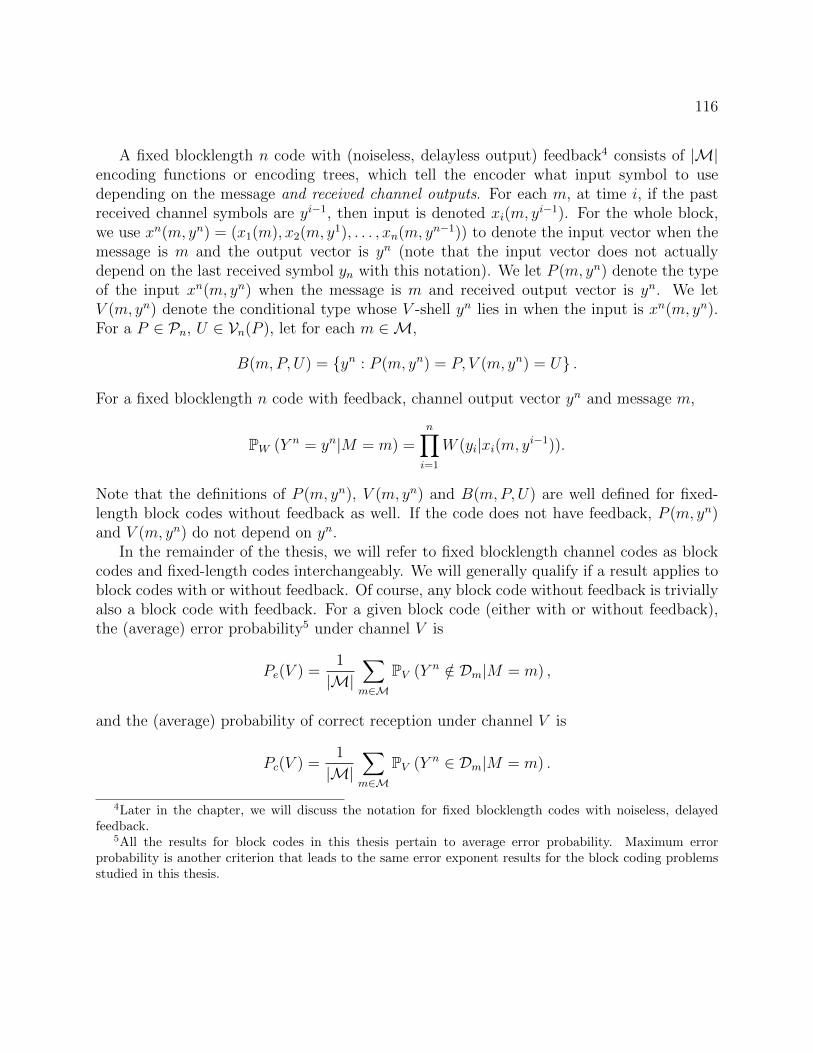
116

A fixed blocklength n code with (noiseless, delayless output) feedback4 consists of |M|encoding functions or encoding trees, which tell the encoder what input symbol to usedepending on the message and received channel outputs. For each m, at time i, if the pastreceived channel symbols are yi−1, then input is denoted xi(m, y

i−1). For the whole block,we use xn(m, yn) = (x1(m), x2(m, y

1), . . . , xn(m, yn−1)) to denote the input vector when themessage is m and the output vector is yn (note that the input vector does not actuallydepend on the last received symbol yn with this notation). We let P (m, yn) denote the typeof the input xn(m, yn) when the message is m and received output vector is yn. We letV (m, yn) denote the conditional type whose V -shell yn lies in when the input is xn(m, yn).For a P ∈ Pn, U ∈ Vn(P ), let for each m ∈M,

B(m,P, U) = yn : P (m, yn) = P, V (m, yn) = U .

For a fixed blocklength n code with feedback, channel output vector yn and message m,

PW (Y n = yn|M = m) =n∏i=1

W (yi|xi(m, yi−1)).

Note that the definitions of P (m, yn), V (m, yn) and B(m,P, U) are well defined for fixed-length block codes without feedback as well. If the code does not have feedback, P (m, yn)and V (m, yn) do not depend on yn.

In the remainder of the thesis, we will refer to fixed blocklength channel codes as blockcodes and fixed-length codes interchangeably. We will generally qualify if a result applies toblock codes with or without feedback. Of course, any block code without feedback is triviallyalso a block code with feedback. For a given block code (either with or without feedback),the (average) error probability5 under channel V is

Pe(V ) =1

|M|∑m∈M

PV (Y n /∈ Dm|M = m) ,

and the (average) probability of correct reception under channel V is

Pc(V ) =1

|M|∑m∈M

PV (Y n ∈ Dm|M = m) .

4Later in the chapter, we will discuss the notation for fixed blocklength codes with noiseless, delayedfeedback.

5All the results for block codes in this thesis pertain to average error probability. Maximum errorprobability is another criterion that leads to the same error exponent results for the block coding problemsstudied in this thesis.

117

A.2 Sphere-packing without feedback via method of

types

Theorem 1 (first part) of Section 2.3: Fix a δ > 0. There is a finite nSP (W, δ) suchthat for n ≥ nSP (W, δ), any block code of length n and rate R without feedback has

− 1

nlogPe(W ) ≤ Esp(R− δ) + δ.

Proof: By basic properties of types, we know that |Pn| ≤ (n+ 1)|X |. We have

|M| =

∣∣∣∣∣ ⋃P∈Pn

M(P )

∣∣∣∣∣ =∑P∈Pn

|M(P )|,

where M(P ) = m ∈M : φ(m) ∈ TP. By the pigeon-hole principle, there must then exista P ∈ Pn (depending on the code) such that

|M(P )| ≥ |M|(n+ 1)|X |

.

Now, we have

Pe(W ) =1

|M|∑m∈M

P(Y n /∈ Dm|Xn = φ(m))

(a)

≥ 1

|M|∑

m∈M(P )

P(Y n /∈ Dm|Xn = φ(m)) (A.1)

(b)=

1

|M|∑

m∈M(P )

∑V ∈Vn(P )

∑yn∈TV (φ(m))∩Dcm

P(Y n = yn|Xn = φ(m))

(c)=

1

|M|∑

m∈M(P )

∑V ∈Vn(P )

∑yn∈TV (φ(m))∩Dcm

exp (−n [D(V ||W |P ) +H(V |P )])

(d)=

1

|M|∑

V ∈Vn(P )

exp (−n [D(V ||W |P ) +H(V |P )])∑

m∈M(P )

∑yn∈TV (φ(m))∩Dcm

1

(e)=

1

|M|∑

V ∈Vn(P )

exp (−n [D(V ||W |P ) +H(V |P )])∑

m∈M(P )

|TV (φ(m)) ∩ Dcm| . (A.2)

In the above, (a) is due to the sum being over fewer non-negative terms, (b) expands theprobability by summing over individual output vectors, (c) follows from the properties ofV -shells, (d) interchanges sums and (e) notes that the innermost sum in (d) is simply thesize of a set. Now, we need to understand when the term

∑m∈M(P ) |TV (φ(m)) ∩ Dcm| is large.

118

Now, ∀ m ∈M(P ), we know |TV (φ(m))| = |TV (φ(m))∩Dm|+ |TV (φ(m))∩Dcm|, so it followsthat ∑

m∈M(P )

|TV (φ(m)) ∩ Dcm| =∑

m∈M(P )

|TV (φ(m))| − |TV (φ(m)) ∩ Dm|

(a)

≥ |M(P )| exp(nH(V |P ))

(n+ 1)|X ||Y|−

∑m∈M(P )

|TV (φ(m)) ∩ Dm|. (A.3)

In the above line, (a) follows by standard properties of V -shells. At this point, note that forall m ∈ M(P ), TV (φ(m)) ∩ Dm are disjoint sets because Dm are disjoint. Furthermore, ifm ∈ M(P ), yn ∈ TV (φ(m)) implies that yn ∈ TPV also, where TPV is the type class of yn

vectors that have type PV . Therefore, we have

∑m∈M(P )

|TV (φ(m)) ∩ Dm| =

∣∣∣∣∣∣⋃

m∈M(P )

TV (φ(m)) ∩ Dm

∣∣∣∣∣∣≤ |TPV |≤ exp(nH(PV )).

Hence, plugging the above inequality into (A.3), we have∑m∈M(P )

|TV (φ(m)) ∩ Dcm| ≥|M(P )| exp(nH(V |P ))

(n+ 1)|X ||Y|− exp(nH(PV ))

(a)

≥ exp(n(R +H(V |P )))

(n+ 1)|X |(1+|Y|)− exp(nH(PV ))

(b)= exp

(n

(R +H(V |P )− |X |(1 + |Y|)

nlog(n+ 1)

))×[

1− exp

(−n(R− I(P, V )− |X |(1 + |Y|)

nlog(n+ 1)

))].

In the above, (a) follows from the fact that |M(P )| is almost as large as |M| (at leastexponentially), and (b) follows by the fact that I(P, V ) = H(PV )−H(V |P ). We want theterm in brackets above to be close to 1, so we restrict the choice of V to those V that have

119

I(P, V ) ≤ R− δ for some small δ > 0. Plugging this into (A.2) gives

Pe(W ) ≥ 1

|M|∑

V ∈Vn(P ):I(P,V )≤R−δ

exp

(−n(D(V ||W |P )−R +

|X |(1 + |Y|)n

log(n+ 1)

))×[

1− exp

(−n[δ − |X |(1 + |Y|)

nlog(n+ 1)

])]=

∑V ∈Vn(P ):I(P,V )≤R−δ

exp

(−n(D(V ||W |P ) +

|X |(1 + |Y|)n

log(n+ 1)

))×[

1− exp

(−n[δ − |X |(1 + |Y|)

nlog(n+ 1)

])]. (A.4)

Now, for n large enough, depending on |X |, |Y| and δ, we have that

(n+ 1)−|X |(1+|Y|)[1− exp

(−n[δ − |X |(1 + |Y|)

nlog(n+ 1)

])]≥ exp(−nδ),

so plugging into (A.4), we have that for n large enough,

Pe(W ) ≥ exp

(−n[

minV ∈Vn(P ):I(P,V )≤R−δ

D(V ||W |P ) + δ

])(a)

≥ exp

(−n[

maxP∈Pn

minV ∈Vn(P ):I(P,V )≤R−δ

D(V ||W |P ) + δ

]).

In the above, (a) follows because we do not know the most populous codeword type a priori,so we take the most optimistic one in terms of the exponent. Now, we have a term thatdepends on n that looks like the sphere-packing exponent. Lemma 6 of Appendix A.12.2tells us that

maxP∈Pn

minV ∈Vn(P ):I(P,V )≤R−δ

D(V ||W |P ) ≤ maxP∈P

minV ∈W:I(P,V )≤R−δ− 2|X||Y|

nlog(n)

D(V ||W |P )

+ κW|X ||Y|n

+|X ||Y|n

log

(n

|X |

)= Esp

(R− δ − 2|X ||Y|

nlog n

)+

κW|X ||Y|n

+|X ||Y|n

log

(n

|X |

),

where

κW = maxx,y:W (y|x)>0

log1

W (y|x).

120

Hence, for n large enough depending6 on κW , |X |, |Y| and δ, we have

Pe(W ) ≥ exp (−n [Esp(R− 2δ) + 2δ]) .

A.3 Sphere-packing without feedback via change of mea-

sure

Theorem 1 (second part) of Section 2.3: For any δ > 0, there exists a finite nsp(W, δ)such that any block code without feedback of rate at least R and length n ≥ nsp(W, δ) has

− 1

nlogPe(W ) ≤ Esp (R− δ) + δ.

Proof: We will use a change-of-measure approach to prove that a high error probabilityunder channel V implies an error probability under channel W involving a divergence termthat is exponentially decaying with the sphere-packing exponent after proper selection ofV . To do so, we will use Lemma 12 in this Appendix and a lemma about what happensto the error probability when we change measures. First, restrict attention to the largestfixed-type subcode of the code being bounded. That is, assume that there is a P ∈ Pn suchthat φ(m) ∈ TP for all m ∈ M. We know from Lemma 12 that if all codewords have thesame type P and R− I(P, V ) ≥ δ > 0,

Pc(V ) ≤ γSC(n, δ, |X |, |Y|)

with γSC being defined in Lemma 12. The critical feature of γSC is that γSC(n, δ, |X |, |Y|)→ 0as n→∞. Now we can apply Lemma 18 of Appendix A.14 to get (since all codewords areassumed to be of type P ∈ Pn),

Pe(W ) ≥ Pe(V ) exp

(−n[D(V ||W |P ) +

maxκV , κWPe(V )

β(n, |X |, |Y|)])

,

where

β(n, |X |, |Y|) = infε>0

ε+ (n+ 1)|X ||Y| exp

(−nε

2

2

).

Therefore,

Pe(W ) ≥ (1− γSC(n, δ, |X |, |Y|))×

exp

(−n[D(V ||W |P ) +

maxκV , κW1− γSC(n, δ, |X |, |Y|)

β(n, |X |, |Y|)])

.

6Note that |X |, |Y| and κW are all quantities that can be derived from W .

121

At this point, we remove the restriction that all message codewords have to be of thesame type. Since there are at most (n+ 1)|X | types of length n for X n, there is at least onetype P that has at least |M|/(n+ 1)|X | codewords. We can apply the previous argument tolower bound Pe(W ) for this subset of messages. This adds a penalty of |X | log(n + 1)/n tothe probability term (to account for the thinning of the code in order to make the precedingargument). Furthermore, we must assume that R − |X | log(n + 1)/n − I(P, V ) = δ > 0in order to apply Lemma 12. In the limit as n → ∞, however, these two penalties can beabsorbed into slack parameters in the exponent. Taking these two points into considerationyields

Pe(W ) ≥ (1− γSC(n, δ, |X |, |Y|))(n+ 1)|X |

×

exp

(−n[D(V ||W |P ) +

maxκV , κW1− γSC(n, δ, |X |, |Y|)

β(n, |X |, |Y|)])

,

where implicitly, we are now restricted to choices of V such that I(P, V ) ≤ R−δ−|X | log(n+1)/n. Optimizing over such V (i.e. setting V to be the sphere-packing optimizing V ∗ for

type P at rate R− δ − |X |n

log(n+ 1)) yields

Pe(W ) ≥ exp

(−n[Esp

(R− δ − |X |

nlog(n+ 1)

)+

maxκV ∗ , κW1− γSC(n, δ, |X |, |Y|)

β(n, |X |, |Y|)])×

(1− γSC(n, δ, |X |, |Y|))(n+ 1)|X |

.

Lemma 1 shows that κV ∗ ≤ κW + log |Y|, and we know that β(n, |X |, |Y|) = O

(√lognn

), so

Pe(W ) ≥ exp

(−n

[Esp

(R− δ − |X |

nlog(n+ 1)

)+

κW + log |Y|1− γSC(n, δ, |X |, |Y|)

O

(√log n

n

)])×

(1− γSC(n, δ, |X |, |Y|))(n+ 1)|X |

.

Since 1n

log(n + 1) → 0 and γSC(n, δ, |X |, |Y|) → 0, it follows that for n large enough,depending on κW , |X |, |Y| and δ,

− 1

nlogPe(W ) ≤ Esp(R− 2δ) + 2δ.

Lemma 12 (Strong converse without feedback). Fix a block code without feedback of lengthn. Suppose there is a P ∈ Pn such that ∀ m ∈ M, φ(m) ∈ TP . Fix an ε ∈ (0, 1/2). Then,

122

for any W ∈ W,

Pc(W ) ≤ exp

(−n[ε2

2− |X ||Y|

nlog(n+ 1)

])+

exp

(−n[R− I(P,W )− 2ε log

|X ||Y|ε− |Y|

nlog(n+ 1)

]).

Therefore, we have

Pc(W ) ≤ γSC(n,R− I(P,W ), |X |, |Y|),

where

γSC(n, δ, |X |, |Y|) = infε∈(0,1/2)

[exp

(−n[ε2

2− |X ||Y|

nlog(n+ 1)

])+

exp

(−n[δ − 2ε log

|X ||Y|ε− |Y|

nlog(n+ 1)

])].

Note that γSC(n,R− I(P,W ), |X |, |Y|)→ 0 as n→∞ for a fixed R− I(P,W ) > 0.

Proof: Fix an ε ∈ (0, 1/2). For each m, define a typical set

Am,ε(W ) = yn : yn ∈ TV (φ(m)), V ∈ Vn(P ), (P, V ) ∈ Jε(W )

Jε(W ) =

(P, V ) ∈ P ×W :

∑x

P (x)∑y

|V (y|x)−W (y|x)| ≤ ε

.

By Lemma 19 of Appendix A.14, we know that for each m,

PW (Y n /∈ Am,ε(W )|Xn = φ(m)) ≤ (n+ 1)|X ||Y| exp(−nε2/2).

123

Now,

Pc(W ) =1

|M|∑m∈M

PW (Y n ∈ Dm|Xn = φ(m))

=1

|M|∑m∈M

PW (Y n ∈ Dm ∩ Am,ε(W )|Xn = φ(m))+

1

|M|∑m∈M

PW (Y n ∈ Dm ∩ Am,ε(W )c|Xn = φ(m))

≤ 1

|M|∑m∈M

PW (Y n ∈ Dm ∩ Am,ε(W )|Xn = φ(m))+

1

|M|∑m∈M

PW (Y n ∈ Am,ε(W )c|Xn = φ(m))

≤ 1

|M|∑m∈M

PW (Y n ∈ Dm ∩ Am,ε(W )|Xn = φ(m))+

(n+ 1)|X ||Y| exp

(−nε

2

2

). (A.5)

Considering just the first term in the bound above, we have

T1 ,1

|M|∑m∈M

PW (Y n ∈ Dm ∩ Am,ε(W )|Xn = φ(m))

=1

|M|∑m∈M

∑V ∈Vn(P ):(P,V )∈Jε(W )

∑yn∈Dm∩TV (φ(m))

PW (Y n = yn|Xn = φ(m))

=1

|M|∑m∈M

∑V ∈Vn(P ):(P,V )∈Jε(W )

∑yn∈Dm∩TV (φ(m))

exp (−n [D(V ||W |P ) +H(V |P )])

=1

|M|∑m∈M

∑V ∈Vn(P ):(P,V )∈Jε(W )

|Dm ∩ TV (φ(m))| exp (−n [D(V ||W |P ) +H(V |P )])

=∑

V ∈Vn(P ):(P,V )∈Jε(W )

exp (−n [D(V ||W |P ) +H(V |P ) +R])∑m∈M

|Dm ∩ TV (φ(m))|

≤∑

V ∈Vn(P ):(P,V )∈Jε(W )

exp (−n [H(V |P ) +R])∑m∈M

|Dm ∩ TV (φ(m))|.

Now, we note that for all V such that (P, V ) ∈ Jε(W ), H(V |P ) is close to H(W |P ), as

124

shown in Proposition 15, so we have

T1 ≤∑

V ∈Vn(P ):(P,V )∈Jε(W )

exp

(−n[H(W |P )− ε log

|X ||Y|ε

+R

]) ∑m∈M

|Dm ∩ TV (φ(m))|

= exp

(−n[H(W |P )− ε log

|X ||Y|ε

+R

]) ∑V ∈Vn(P ):(P,V )∈Jε(W )

∑m∈M

|Dm ∩ TV (φ(m))|

= exp

(−n[H(W |P )− ε log

|X ||Y|ε

+R

])|Aε(W )| ,

where we have defined the union of the message-typical sets to be

Aε(W ) =⋃m∈M

Am,ε(W ).

From Proposition 7, we know that

|Aε(W )| ≤ (n+ 1)|Y| exp

(n

[H(PW ) + ε log

|Y|ε

]).

Hence,

T1 ≤ (n+ 1)|Y| exp

(−n[H(W |P )−H(PW )− 2ε log

|X ||Y|ε

+R

])= (n+ 1)|Y| exp

(−n[R− I(P,W )− 2ε log

|X ||Y|ε

]).

Plugging the bound above back into equation (A.5) gives the result of the lemma.

Proposition 7. Let PW denote the distribution induced on Y by the distribution P on Xwith channel W , that is (PW )(y) =

∑x P (x)W (y|x). Then,

|Aε(W )| ≤ (n+ 1)|Y| exp

(n

[H(PW ) + ε log

|Y|ε

]).

Proof: If yn ∈ Am,ε(W ), then yn ∈ TV (φ(m)) for some V ∈ Vn(P ) with∑x

P (x)∑y

|V (y|x)−W (y|x)| ≤ ε.

This also implies that yn ∈ TPV ⊂ Yn, where PV ∈ Qn. Now, since V is not far fromW , we can show that PV is not far from PW .∑

y

|(PV )(y)− (PW )(y)| =∑y

∣∣∣∣∣∑x

P (x)V (y|x)− P (x)W (y|x)

∣∣∣∣∣≤∑x

P (x)∑y

|V (y|x)−W (y|x)|

≤ ε.

125

Since we have assumed that ε ∈ (0, 1/2), we can apply Lemma 20 of Appendix A.14 todeduce that

|H(PV )−H(PW )| ≤ ε log|Y|ε.

Hence, if yn ∈ Aε(W ), we also have yn ∈ TQ for some Q ∈ Qn with |H(Q) − H(PW )| ≤ε log |Y|

ε. Therefore, by standard properties of types,

|Aε(W )| =⋃m∈M

Am,ε(W )

≤⋃Q∈Qn

|TQ|

≤ (n+ 1)|Y| exp

(n

[H(PW ) + ε log

|Y|ε

]).

A.4 Haroutunian exponent for fixed-length codes with

feedback

Theorem 2 of Section 2.3: For any δ > 0, there exists a finite nh(W,R, δ) such that anyfixed-length code with feedback of rate R and length n ≥ nh(W,R, δ) has

− 1

nlogPe(W ) ≤ Eh(R− δ) + δ.

Proof: We will use Lemma 13 of this Appendix to show that if the capacity of a testchannel V is too small, the error probability will be high. Then, we will use a change-of-measure argument to show that the error probability under channel W will be the errorprobability under V multiplied by an exponentially decaying divergence term that corre-sponds to the Haroutunian exponent. Fix a test channel V . We know from Lemma 13 thatif R− C(V ) = δ > 0,

Pc(V ) ≤ γSC,fb(n, δ, |X |, |Y|)

with γSC,fb being defined in Lemma 13. The critical feature of γSC,fb is that γSC,fb(n, δ, |X |, |Y|)→0 as n→∞. At this point, we apply Lemma 18 to get

Pe(W ) ≤ Pe(V ) exp

(−n[maxP

D(V ||W |P ) +maxκV , κW

Pe(V )β(n, |X , |Y|)

]),

where

β(n, |X |, |Y|) = infε>0

ε+ (n+ 1)|X ||Y| exp

(−nε

2

2

).

126

If we let V be V ∗, where

V ∗ ∈ arg minV :C(V )≤R−δ

maxP

D(V ||W |P ),

then

Pe(W ) ≥ exp

(−n[Eh(R− δ) +

maxκV ∗ , κW1− γSC,fb(n, δ, |X |, |Y|)

β(n, |X , |Y|)])×

(1− γSC,fb(n, δ, |X |, |Y|)).

Now, β(n, |X |, |Y|) = O

(√lognn

), and γSC,fb(n, δ, |X |, |Y|) → 0, so for n large enough

depending on W , R and δ,

− 1

nlogPe(W ) ≤ Eh(R− δ) + δ.

Lemma 13. Let C(W ) = maxP∈P I(P,W ) be the capacity of W . Then, for a fixed-lengthblock code used with feedback of length n and rate R, and any ε ∈ (0, 1/2),

Pc(w) ≤ exp

(−n[ε2

2− |X ||Y|

nlog(n+ 1)

])+

exp

(−n[R− C(W )− 2ε log

|X ||Y|ε− |X ||Y|

nlog(n+ 1)

]).

Therefore,

Pc(W ) ≤ γSC,fb(n,R− C(W ), |X |, |Y|),

where

γSC,fb(n, δ, |X |, |Y|) , infε∈(0,1/2)

exp

(−n[ε2

2− |X ||Y|

nlog(n+ 1)

])+

exp

(−n[δ − 2ε log

|X ||Y|ε− |X ||Y|

nlog(n+ 1)

]).

Note that γSC,fb(n,R−C(W ), |X |, |Y|)→ 0 as n→∞ if R−C(W ) > 0 is fixed, and hencethe probability of correct reception goes to 0 if R < C(W ).

Proof: Fix an ε ∈ (0, 1/2). Define for each m, a typical set for the encoding tree ofmessage m,

Am,ε(W ) , yn : (P (m, yn), V (m, yn)) ∈ Jε(W )

Jε(W ) ,

(P, V ) ∈ P ×W :

∑x∈X

P (x)∑y∈Y

|V (y|x)−W (y|x)| ≤ ε

.

127

Recall that P (m, yn) ∈ Pn is the type of input for message m along the output sequence7 yn.That is, P (m, yn) is the type of xn(m, yn) , (x1(m), x2(m, y

1), x3(m, y2), . . . , xn(m, yn−1)),

where yk denotes the first k entries of the vector yn. Accordingly, V (m, yn) is the conditionalshell that yn lies in when viewed from the input xn(m, yn), i.e. yn ∈ TV (m,yn)(x

n(m, yn)).Now,

Pc(W ) =1

|M|∑m∈M

PW (Y n ∈ Dm|M = m)

=1

|M|∑m∈M

PW (Y n ∈ Dm ∩ Am,ε(W )|M = m)

+1

|M|∑m∈M

PW (Y n ∈ Dm ∩ Am,ε(W )c|M = m)

≤ 1

|M|∑m∈M

PW (Y n ∈ Dm ∩ Am,ε(W )|M = m)

+1

|M|∑m∈M

PW (Y n ∈ Am,ε(W )c|M = m)

≤

[1

|M|∑m∈M

PW (Y n ∈ Dm ∩ Am,ε(W )|M = m)

]+ (n+ 1)|X ||Y| exp

(−nε

2

2

).

where the last line is arrived at by Lemma 19. Restricting attention to the first term above,

T1 ,1

|M|∑m∈M

PW (Y n ∈ Dm ∩ Am,ε(W )|M = m)

= exp(−nR)∑m∈M

PW (Y n ∈ Dm ∩ Am,ε(W )|M = m). (A.6)

For each m and P ∈ Pn, V ∈ Vn(P ), recall the ’conditional shell with feedback’

B(m,P, V ) , yn : P (m, yn) = P, V (m, yn) = V .7When feedback is available, the channel input codeword and hence the channel input type depends on

both the message and the received channel symbols.

128

Bounding further using this definition,

T2 ,∑m∈M

PW (Y n ∈ Dm ∩ Am,ε(W )|M = m)

=∑m∈M

∑(P,V )∈Jε(W )

PW (Y n ∈ B(m,P, V ) ∩ Dm|M = m)

(a)=∑m∈M

∑(P,V )∈Jε(W )

|B(m,P, V ) ∩ Dm| exp (−n [D(V ||W |P ) +H(V |P )])

=∑

(P,V )∈Jε(W )

exp (−n [D(V ||W |P ) +H(V |P )])∑m∈M

|B(m,P, V ) ∩ Dm|

(b)

≤∑

(P,V )∈Jε(W )

exp (−n [D(V ||W |P ) +H(V |P )]) exp(nH(PV ))

(c)

≤∑

(P,V )∈Jε(W )

exp(nI(P, V )), (A.7)

where in the above, (a) follows from Proposition 14b, (b) follows from Proposition 14a andthe fact that the decoding regions are disjoint, and (c) follows from divergence being non-negative and I(P, V ) = H(PV ) −H(V |P ). From Proposition 15, we know that I(P, V ) ≤I(P,W ) + 2ε log(|X ||Y|/ε) for (P, V ) ∈ Jε(W ), so plugging (A.7) into (A.6), and taking themax over P ∈ P yields

T1 ≤ (n+ 1)|X ||Y| exp

(−n[R−max

P∈PI(P,W )− 2ε log

|X ||Y|ε

])= exp

(−n[R− C(W )− 2ε log

|X ||Y|ε− |X ||Y|

nlog(n+ 1)

]).

So, for any ε ∈ (0, 1/2), we have shown that

Pc(W ) ≤ exp

(−n[ε2

2− |X ||Y|

nlog(n+ 1)

])+

exp

(−n[R− C(W )− 2ε log

|X ||Y|ε− |X ||Y|

nlog(n+ 1)

]).

Optimizing over ε ∈ (0, 1/2) yields the desired result.

A.5 A special family of test channels

Lemma 1 of Section 2.4:

129

Let P (V ) be any continuous function from W to P , and let for any V ∈ W ,

κV = maxx,y:V (y|x)>0

log(1/V (y|x)).

Then, for all R > 0, ε > 0,

infV :I(P (V ),V )≤R

D(V ||W |P (V )) + εmax κV , κW ≤ Esp(R) + ε(κW + log |Y|).

Proof: This result is due to Baris Nakiboglu. It can be used to fill in an apparent gap inthe proof of Sheverdyaev’s result (although there is another issue with that paper, as notedin Appendix A.7). Recall that the sphere-packing exponent has two forms ( [18], [47]):

Esp(R) = maxP∈P

minV :I(P,V )≤R

D(V ||W |P )

Esp(R) = supρ≥0

E0(ρ)− ρR

E0(ρ) , maxP∈P− log

∑y

(∑x

P (x)W (y|x)1/(1+ρ)

)1+ρ

= − log minP∈P

∑y

(∑x

P (x)W (y|x)1/(1+ρ)

)1+ρ

= − log minP∈P

f(P, ρ)

f(P, ρ) ,∑y

(∑x

P (x)W (y|x)1/(1+ρ)

)1+ρ

.

Let

P∗ρ , arg minP∈P

f(P, ρ).

It is known that f(P, ρ) is convex in P [16] and therefore, for each ρ ≥ 0, P∗ρ is either aunique distribution in P or a convex region of distributions in P . Further, for every ρ, itcan be shown ( [47], Problem 2.5.23(iv)) that P ∈ P∗ρ if and only if, for all x ∈ X ,

∑y

W (y|x)1/(1+ρ)

[∑x′

P (x′)W (y|x′)1/(1+ρ)]ρ≥∑y

(∑x′

P (x′)W (y|x′)1/(1+ρ))1+ρ

, (A.8)

with equality for all x such that P (x) > 0.

Proposition 8. There exists a parametrized family of distributions

Pδδ≥0 ⊂ P

and a continuous, monotone nondecreasing map g : [0,∞)→ [0,∞) such that

130

(a) Pδ is continuous as a function of δ

(b) Pδ satisfies the condition in (A.8) for ρ = g(δ)

(c) g(0) = 0, and limδ→∞ g(δ) =∞

The idea is that for each ρ, there is either a unique optimizer or a convex set of optimizersfor f(P, ρ). The problem is to make sure that we get a continuous family of Pδ that are eachoptimizers for a ρ. This is a subtle issue because a priori we have no information about howmany ρ have optimizers which are actually sets and not unique elements. We will see thatthis distinction is equivalent to the fact that E0(ρ) may be nondifferentiable at some points.

First, define for ρ, ε ≥ 0,

P[ρ,ε] ,

(P, s) ∈ P × [0,∞) : |f(P, s)− E0(ρ)| < ε,∃ P ′ ∈ P∗ρ s.t. ||(P, s)− (P ′, ρ)||1 < ε.

Although f(P, ρ) is convex in P and ρ, it is not necessarily convex in both at the same time.Therefore, when taking the minimum over P , it may not be differentiable in ρ. Therefore,even though E0(ρ) is continuous, monotone nondecreasing and concave [16], it can be non-differentiable in places. However, there is a way to bridge optimizers when this happens.Define the sets

P−[ρ,ε],γ , P∗ρ

⋂ ⋂s∈(ρ−γ,ρ)

P[s,ε]

P−ρ , lim

ε→0limγ→0P−[ρ,ε],γ.

Similarly, for the other side, define P+ρ . By continuity of f(P, ρ), we know that both P+

ρ

and P−ρ are non empty. If their intersection is nonempty, we will choose one element fromthe intersection and call it Pδ for some δ that will be clear with g(δ) = ρ. If not, we willtake one element from each, call them P+

ρ and P−ρ and construct a convex combinationβP−ρ + (1 − β)P+

ρ = Pρ,β. Note that by convexity, Pρ,β ∈ Pρ. Also, when the intersectionbetween P+

ρ and P−ρ is nonempty, Pρ is continuous, and when the intersection is empty, wecan construct an arbitrary positive length continuous segment going from P−ρ to P+

ρ . Weuse the monotonically nondecreasing function g to account for these gaps.

Now, the only thing that remains to be checked is that the number of points at whichE0(ρ) is nondifferentiable is countable so that such a function g exists. To see this, werecall that E0(ρ) is continuous and concave. Therefore, its derivative is monotonic andnonincreasing where it exists (assign it to be the upper derivative at points of discontinuity).It is easy to see however, that the set of discontinuities for a monotonic function is countable(otherwise the jumps add up too fast). Therefore, a function g as the proposition requiresexists to map the δ to ρ parametrically and in a monotonic way. Note that g will not beone-to-one if E0(ρ) is ever nondifferentiable.

131

From now on, for a given δ ≥ 0, let ρ = g(δ) be parametrically defined through δ and g.Define, for each δ > 0, a channel

Vδ(y|x) ,W (y|x)1/(1+ρ)

(∑x′ Pδ(x

′)W (y|x′)1/(1+ρ))ρ∑

y′W (y′|x)1/(1+ρ) (∑

x′ Pδ(x′)W (y′|x′)1/(1+ρ))ρ

(A.9)

r(x, δ) ,∑y′

W (y′|x)1/(1+ρ)

(∑x′

Pδ(x′)W (y′|x′)1/(1+ρ)

)ρ

.

Note, by (A.8), we have for all x, δ,

r(x, δ) ≥∑y

(∑x

Pδ(x′)W (y|x)1/(1+ρ)

)1+ρ

= exp (−E0(ρ)) (A.10)

where the last line follows because Pδ is a member of P∗ρ . Also, r(x, δ) = exp(−E0(ρ)) for xsuch that Pδ(x) > 0. Now, fix a δ ≥ 0 and consider D(Vδ||W |P ) for an arbitrary P ∈ P .

D(Vδ||W |P ) =∑x,y

P (x)Vδ(y|x) logVδ(y|x)

W (y|x)

(a)=∑x,y

P (x)Vδ(y|x) logVδ(y|x)

Vδ(y|x)1+ρ exp(−(1+ρ)E0(ρ))

(∑′x Pδ(x

′)W (y|x′)1/(1+ρ))ρ(1+ρ)

(b)

≤∑x,y

P (x)Vδ(y|x) log

[((∑x′ Pδ(x

′)W (y|x′)1/(1+ρ))1+ρ

Vδ(y|x)e−E0(ρ)

)ρ

eE0(ρ)

],

where (a) follows by inversion of (A.9) and (b) from (A.10).

D(Vδ||W |P ) ≤ E0(ρ) + ρ∑x,y

P (x)Vδ(y|x) log

(∑x′ Pδ(x

′)W (y|x′)1/(1+ρ))1+ρ

Vδ(y|x)e−E0(ρ)

= E0(ρ)− ρ∑x,y

P (x)Vδ(y|x) log

[Vδ(y|x)

(PVδ)(y)× (PVδ)(y)e−E0(ρ)

(∑

x′ Pδ(x′)W (y|x′)1/(1+ρ))1+ρ

]= E0(ρ)− ρI(P, Vδ)−

ρ∑x,y

P (x)Vδ(y|x) log

((PVδ)(y)

(∑

x′ Pδ(x′)W (y|x′)1/(1+ρ))1+ρ /e−E0(ρ)

).

(A.11)

132

Now, let Qδ(x|y) be the conditional distribution defined by

Qδ(x|y) =P (x)Vδ(y|x)

(PVδ)(y).

Then, picking up from (A.11),

D(Vδ||W |P ) ≤ E0(ρ)− ρ(I(P, Vδ))−

ρ∑x,y

P (x)Vδ(y|x) log

(Qδ(x|y)(PVδ)(y)

Qδ(x|y) (∑

x′ Pδ(x′)W (y|x′)1/(1+ρ))1+ρ /e−E0(ρ)

).

Now, note that

∑y

(∑x

Pδ(x)W (y|x)1/(1+ρ)

)1+ρ

= e−E0(ρ)

Therefore, (∑x′ Pδ(x

′)W (y|x′)1/(1+ρ))1+ρ

e−E0(ρ)

is a distribution on Y since for each y, it is nonnegative and sums to one over Y . Call thisdistribution Qδ ∈ Q. Then, we have

D(Vδ||W |P ) ≤ E0(ρ)− ρ(I(P, Vδ))−

ρ∑x,y

P (x)Vδ(y|x) log

(Qδ(x|y)(PVδ)(y)

Qδ(x|y)Qδ(y)

)= E0(ρ)− ρ(I(P, Vδ))−

ρ∑x,y

P (x)Vδ(y|x) log

(P (x)Vδ(y|x)

Qδ(x|y)Qδ(y)

)(c)

≤ E0(ρ)− ρI(P, Vδ)

≤ supρ≥0

E0(ρ)− ρI(P, Vδ)

= Esp(I(P, Vδ)), (A.12)

where (c) follows because the term that was eliminated was a divergence and hence nonneg-

133

ative. Now,

infV :I(PV ,V )≤R

D(V ||W |PV ) ≤ infVδ,δ≥0:I(PVδ ,Vδ)≤R

D(Vδ||W |PVδ)

(d)

≤ infVδ,δ≥0:I(PVδ ,Vδ)≤R

Esp(I(PVδ , Vδ))

(e)

≤ Esp

(sup

Vδ,δ≥0:I(PVδ ,Vδ)≤RI(PVδ , Vδ)

),

where (d) is true because of (A.12) and (e) follows because Esp(R) is a monotonically non-increasing function of R. Now, Vδ is continuous in δ by Proposition 8 and (A.9). Byassumption, PV is continuous in V , so PVδ is continuous in δ. Further, I(P, V ) is continuousin the pair P, V , so I(PVδ , Vδ) is continuous in δ. Note that V0 = W by definition. As δ →∞,it follows that (because ρ = g(δ)→∞, Vδ → V ∗ where for each x,

V ∗(y|x) =1

|y : W (y|x) > 0|.

We claim that

limδ→∞

C(Vδ) = C(V ∗)

= infR : Esp(R) <∞.

That the limit of capacities is equal to the capacity of the limit is clear because capacity isa continuous function of the channel and Vδ converges to V ∗ for a suitable norm (such as L1

norm). Also, note that these Vδ are the channels that are sufficient to upper bound for thesphere-packing exponent ( [47], Problem 2.5.23a), so limδ→∞C(Vδ) ≤ infR : Esp(R) <∞.Conversely, if Esp(R) =∞, since D(V ∗||W |P ) <∞ for all P ∈ P , it follows that C(Vδ) > R.Therefore limδ→∞C(Vδ) = infR : Esp(R) <∞.

Now, returning to the quantity of interest supδ≥0 I(PVδ , Vδ), by the intermediate valuetheorem applied to the continuous function I(PVδ , Vδ), whose endpoints are at I(P,W ) andinfR : Esp(R) <∞, we must have one of two things.

(i) I(PVδ , Vδ) < R for all δ > 0

(ii) There is a δ∗ such that I(PVδ∗ , Vδ∗) = R

In case (i), it is true that I(P,W ) < R, so by Fano’s inequality, the error exponent is assmall as desired for large enough n. In case (ii), we have

infV :I(PV ,V )≤R

D(V ||W |PV ) ≤ Esp(R) + εmax κVδ∗ , κW .

134

Now, note that if θW = minx,y:W (y|x)>0W (y|x), and x, y is such that W (y|x) > 0, we havefor any δ ≥ 0

Vδ(y|x) ,W (y|x)1/(1+ρ)

(∑x′ Pδ(x

′)W (y|x′)1/(1+ρ))ρ∑

y′W (y′|x)1/(1+ρ) (∑

x′ Pδ(x′)W (y′|x′)1/(1+ρ))ρ

≥ θW θρ/(1+ρ)W∑′y 1

=θW|Y|

κVδ ≤ κW + log |Y|.

which concludes the proof of the lemma. .

A.6 Failed Approaches to proving the sphere packing

bound for codes with feedback

A.6.1 A first attempt via Fano’s inequality

Lemma 2 of Section 2.4.1: Fix an R > 0 and δ ∈ (1/n,R). For any block code withfeedback of rate R and length n,

− 1

nlogPe(W ) ≤ inf

V :I(PV ,V )≤R−δD(V ||W |PI,V )+

2 maxκV , κW1R

(δ − 1

n

) β(n, |X |, |Y|) +1

nlog

(1

R

(δ − 1

n

)),

where

β(n, |X |, |Y|) = infε>0

ε+ (n+ 1)|X ||Y| exp

(−nε

2

2

).

Proof: Fix a V such that I(PV , V ) ≤ R − δ, with δ ∈ (1/n,R). From Proposition 9, weknow that

Pe(V ) ≥ 1

R

(δ − 1

n

). (A.13)

Then, from Lemma 18 in Appendix A.14,

Pe(W ) ≥ Pe(V ) exp (−nd(V,W )) ,

135

where

d(V,W ) =1

|M|∑m∈M

∑yn∈Dcm

PV (Y n = yn|M = m)

Pe(V )

1

n

n∑i=1

logV (yi|xi(m, yi−1))W (yi|xi(m, yi−1))

.

Now, recalling that B(m,P, U) = yn : P (m, yn) = P, V (m, yn) = U, we have

d(V,W ) =1

|M|∑

m∈M,P∈Pn,U∈Vn(P )

∑yn∈Dcm∩B(m,P,U)

PV (Y n = yn|M = m)

Pe(V )×

∑x,y

P (x)U(y|x) logV (y|x)

W (y|x)

=1

|M|∑

m∈M,P∈Pn,U∈Vn(P )

∑yn∈Dcm∩B(m,P,U)

PV (Y n = yn|M = m)

Pe(V )×[

D(V ||W |P ) +∑x,y

P (x)(U(y|x)− V (y|x)) logV (y|x)

W (y|x)

].

A little bit of algebra and linearity of D(V ||W |P ) in P shows that

1

|M|∑

m∈M,P∈Pn,U∈Vn(P )

∑yn∈Dcm∩B(m,P,U)

PV (Y n = yn|M = m)

Pe(V )D(V ||W |P ) = D(V ||W |PI,V ),

so we need to control the difference term. For ε > 0, let

Jε(V ) =

(P,U) ∈ P ×W :

∑x

P (x)∑y

|U(y|x)− V (y|x)| ≤ ε

.

136

Then, splitting the difference term into ‘typical’ and ‘atypical’ parts gives

T ,1

|M|∑

m∈M,P∈Pn,U∈Vn(P )

∑yn∈Dcm∩B(m,P,U)

PV (Y n = yn|M = m)

Pe(V )×

∑x,y

P (x)(U(y|x)− V (y|x)) logV (y|x)

W (y|x)

= T1 + T2

T1 ,1

|M|∑

m∈M,P∈Pn,U∈Vn(P ):(P,U)∈Jε(V )

∑yn∈Dcm∩B(m,P,U)

PV (Y n = yn|M = m)

Pe(V )×

∑x,y

P (x)(U(y|x)− V (y|x)) logV (y|x)

W (y|x)

T2 ,1

|M|∑

m∈M,P∈Pn,U∈Vn(P ):(P,J)/∈Jε(V )

∑yn∈Dcm∩B(m,P,U)

PV (Y n = yn|M = m)

Pe(V )×

∑x,y

P (x)(U(y|x)− V (y|x)) logV (y|x)

W (y|x).

Now, by Proposition 13, if (P,U) ∈ Jε(V ), we have∑x,y

P (x)(U(y|x)− V (y|x)) logV (y|x)

W (y|x)≤ εmaxκV , κW,

for all the terms in T1 that contribute something non-zero to the sum. That is, if P(Y n =yn|M = m) = 0, then it does not matter if the difference is infinite. Hence,

T1 ≤ εmaxκV , κW.

As for term T2, sinceD(V ||W |PI,V ) <∞ by assumption,∑

x,y P (x)(U(y|x)−V (y|x)) log V (y|x)W (y|x) <

∞ for all terms in the sum that are not 0. By Lemma 19, we know that for each m ∈M,∑P∈Pn,U∈Vn(P ):(P,U)/∈Jε(V )

PV (Y n ∈ B(m,P, U)|M = m) ≤ (n+ 1)|X ||Y| exp

(−nε

2

2

).

Therefore, because∑

y |U(y|x)− V (y|x)| ≤ 2 for all x and U, V ∈ W ,

T2 ≤2 maxκV , κW

Pe(V )exp

(−n[ε2

2− |X ||Y|

nlog(n+ 1)

]).

Combining the bounds for T1 and T2 tells us that

T ≤ 2 maxκV , κWPe(V )

[ε+ (n+ 1)|X ||Y| exp

(−nε

2

2

)].

Optimizing over ε > 0 gives us the result of the lemma with β(n, |X |, |Y|).

137

Proposition 9 (Fano’s inequality for codes with feedback). If for some V ∈ W, I(PV , V ) ≤R− δ for a rate R length n block code with feedback, then

Pe(V ) ≥ 1

R

(δ − 1

n

).

Proof: First, we will show that if I(PV , V ) ≤ R− δ, then 1nI(M ;Y n) ≤ R− δ also8. For

two random variables A,B on the product set A× B, recall that the mutual information is

I(A;B) =∑

(a,b)∈A×B

P(A = a,B = b) logP(A = a,B = b)

P(A = a)P(B = b)

= H(A)−H(A|B),

where H(A) denotes the entropy of A and H(A|B) denotes the conditional entropy of Agiven B. Using standard properties of the mutual information of a collection of randomvariables (see [21]),

1

nI(M ;Y n) =

1

n(H(Y n)−H(Y n|M))

=1

n

n∑i=1

(H(Yi|Y i−1)−H(Yi|M,Y i−1)

)=

1

n

n∑i=1

I(M ;Yi|Y i−1)

(a)

≤ 1

n

n∑i=1

I(Xi;Yi|Y i−1),

where (a) follows because given Y i−1, M and Yi are conditionally related through Xi. Thatis,

PV (M = m,Xi = x, Yi = y|Y i−1 = yi−1) = PV (M = m|Y i−1 = yi−1)×[1(xi(m, y

i−1) = xi)V (yi|xi)].

8The probabilities in this proposition are all with respect to the measure induced by V .

138

Continuing and expanding the conditional mutual information,

1

nI(M ;Y n) ≤ 1

n

n∑i=1

I(Xi;Yi|Y i−1)

=1

n

n∑i=1

∑yi−1

PV (yi−1)I(Xi;Yi|Y i−1 = yi−1)

=1

n

n∑i=1

∑yi−1

PV (yi−1)I(Pyi−1 , V )

∀ x ∈ X , Pyi−1(x) ,∑m∈M

PV (M = m|Y i−1 = yi−1)1(xi(m, yi−1) = x).

At this point, we can use concavity of mutual information in the input distribution to show

1

nI(M ;Y n) ≤ 1

n

n∑i=1

∑yi−1

PV (yi−1)I(Pyi−1 , V )

≤ I

1

n

n∑i=1

∑yi−1

PV (yi−1)Pyi−1 , V

.

However, noting that

1

n

n∑i=1

∑yi−1

PV (yi−1)Pyi−1 = PV ,

we have shown that 1nI(M ;Y n) ≤ I(PV , V ) ≤ R − δ for a code with feedback. Now, by

Fano’s inequality (see [21], Theorem 2.11.1), we have

H(M |Y n) ≤ hb(Pe(V )) + log(|M| − 1)Pe(V )

≤ 1 + nRPe(V ).

Now, we also have that

H(M |Y n) = H(M)− I(M ;Y n)

≥ nR− n(R− δ) = nδ.

Therefore,

nδ ≤ 1 + nRPe(V )

Pe(V ) ≥ 1

R

(δ − 1

n

).

139

A.6.2 A refined strong converse

Lemma 3 of Section 2.4.2: If the refined strong converse holds, then for any R > 0,δ ∈ (0, R), there is a finite nRSC(W,R, δ) such that for any block code with feedback of rateR and length n ≥ nRSC(W,R, δ),

− 1

nlogPe(W ) ≤ Esp(R− δ) + δ.

Hence, if the refined strong converse holds, so does the sphere-packing bound.Proof: Fix a V such that I(PV , V ) ≤ R− δ. From the proof of Lemma 2, we know that

Pe(W ) ≥ Pe(V ) exp

(−n[D(V ||W |PI,V ) +

2 maxκV , κWPe(V )

β(n, |X |, |Y|)])

,

where PI,V is defined in (2.15) and

β(n, |X |, |Y|) = infε>0

ε+ (n+ 1)|X ||Y| exp

(−nε

2

2

).

From the assumption that the refined strong converse holds, we have

Pe(V ) ≥ 1− γRSC(n, δ, R, κV ).

Now, we claim that since the error event has high probability as γRSC(n, δ, R, κV ) → 0, itmust be that PV is close to PI,V and hence D(V ||W |PV ) is close to D(V ||W |PI,V ).

||PV − PI,V ||1 =∑x∈X

|PV (x)− PI,V (x)|

=∑x∈X

|(Pc(V )PC,V (x) + Pe(V )PI,V (x))− PI,V (x)|

=∑x∈X

|Pc(V )PC,V (x)− Pc(V )PI,V (x)|

= Pc(V )∑x∈X

|PC,V (x)− PI,V (x)|

≤ Pc(V )∑x∈X

PC,V (x) + PI,V (x)

≤ 2Pc(V ) ≤ 2γRSC(n, δ, R, κV ), (A.14)

where the ‘correct input distribution’ is

PC,V (x) ,1

|M|∑m∈M

∑yn∈Dm

PV (Y n = yn|M = m)

Pc(V )

1

n

n∑i=1

1(xi(m, yi−1) = x). (A.15)

140

Now,

D(V ||W |PI,V )−D(V ||W |PV ) =∑x,y

PI,V (x)V (y|x) logV (y|x)

W (y|x)− PV (x)V (y|x) log

V (y|x)

W (y|x)

=∑x,y

(PI,V (x)− PV (x))V (y|x) logV (y|x)

W (y|x)

≤∑x,y

|PI,V (x)− PV (x)|V (y|x) max κV , κW

= ||PI,V − PV ||1 max κV , κW≤ 2γRSC(n, δ, R, κV ) max κV , κW

provided that V (y|x) = 0 whenever W (y|x) = 0. Therefore,

D(V ||W |PI,V ) ≤ D(V ||W |PV ) + 2γRSC(n, δ, R, κV ) max κV , κW .

So, if I(PV , V ) ≤ R− δ,

Pe(W ) ≥ exp

(−n[D(V ||W |P ) +

2 maxκV , κW1− γRSC(n, δ, R, κV )

(β(n, |X |, |Y|) + 2γRSC(n, δ, R, κV ))

])×

(1− γRSC(n, δ, R, κV )).

Now, we optimize over all V such that I(PV , V ) ≤ R− δ. From Lemma 1, we know thatfor the family of sphere-packing optimizing V ’s, κV ≤ κW + log |Y|, so

− 1

nlogPe(W ) ≤ inf

V :I(PV ,V )≤R−δD(V ||W |PV ) +

1

nlog(1− γRSC(n, δ, R, κV ))+

2 maxκV , κW1− γRSC(n, δ, R, κV )

(β(n, |X |, |Y|) + 2γRSC(n, δ, R, κV ))

≤ Esp(R− δ) +1

nlog(1− γRSC(n, δ, R, κW + log |Y|))+

2(κW + log |Y|)1− γRSC(n, δ, R, κW + log |Y|)

×

(β(n, |X |, |Y|) + 2γRSC(n, δ, R, κW + log |Y|)).

Since β(n, |X |, |Y|)→ 0 as n→∞, and γRSC(n, δ, R, κW +log |Y|)→ 0 as n→∞ (assumingthe refined strong converse holds), it follows that for large enough n (depending on W , Rand δ),

− 1

nlogPe(W ) ≤ Esp(R− δ) + δ.

141

A.6.3 A test channel with memory

Lemma 4 of Section 2.4.3: Let V be a measure9 on M×Yn. Fix a δ > 0. Let10

A ,

(m, yn) :

1

nlog

PV (Y n = yn|M = m)

PV (Y n = yn)≤ R− δ

(A.16)

B ,

(m, yn) :

1

nlog

PV (Y n = yn|M = m)

PW (Y n = yn|M = m)≤ Esp(R− 2δ) + δ

(A.17)

E , (m, yn) : yn /∈ Dm .

Then,

Pe(W ) ≥ exp (−n [Esp(R− 2δ) + δ])[1− exp(−nδ)− PV (Bc)− PV (Ac)

].

Hence,

Pe(W ) ≥ exp(−n[Esp(R− 2δ) + 2δ])

for large n provided

PV

(1

nlog

PV (Y n|M)

PV (Y n)≤ R− δ

)→ 1, n→∞ (A.18)

PV

(1

nlog

PV (Y n|M)

PW (Y n|M)≤ Esp(R− 2δ) + δ

)→ 1, n→∞. (A.19)

Proof: The proof of this lemma is essentially the same as the proof of the information-spectrum converse. The only difference is the addition of the set B to make sure thatthe error event under channel V has a high enough probability under channel W . In theinformation spectrum vernacular, log(PV (Y n|M)/PV (Y n)) would be the information densityrandom variable and log(PV (Y n|M)/PW (Y n|M)) would be the divergence density randomvariable. Now,

Pe(W ) = PW (E)

≥ PW (E ∩B)

=∑

(m,yn)∈E∩B

1

|M|PW (Y n = yn|M = m)

(a)

≥∑

(m,yn)∈E∩B

1

|M|PV (Y n = yn|M = m) exp(−n(Esp(R− 2δ) + δ))

= exp(−n(Esp(R− δ) + δ))PV ((M,Y n) ∈ B ∩ E) . (A.20)

9Of course, this measure is induced from one on M×Xn × Yn.10Recall that capital letters are used to denote random variables while lower case vectors denote nonrandom

variables.

142

In the above, (a) follows from the definition of B in (2.19). Now,

PV (B ∩ E) = 1− PV ((B ∩ E)c)

= 1− PV (Bc ∪ Ec)

≥ 1− PV (Bc)− PV (Ec). (A.21)

Now,

PV (Ec) =∑

(m,yn)∈Ec

1

|M|PV (yn|m)

=∑

(m,yn)∈Ec∩A

1

|M|PV (yn|m) +

∑(m,yn)∈Ec∩Ac

1

|M|PV (yn|m)

(b)

≤∑

(m,yn)∈Ec∩A

exp(n(R− δ))|M|

PV (yn) +∑

(m,yn)∈Ec∩Ac

1

|M|PV (yn|m)

= exp(−nδ)∑

(m,yn)∈Ec∩A

PV (yn) +∑

(m,yn)∈Ec∩Ac

1

|M|PV (yn|m)

(c)

≤ exp(−nδ) +∑

(m,yn)∈Ec∩Ac

1

|M|PV (yn|m)

≤ exp(−nδ) + PV (Ac), (A.22)

where (b) follows from the definition of A in (A.16) and (c) follows because each yn appearsin at most one Dm by the definition of decoding regions. Plugging (A.22) into (A.21) and(A.21) into (A.20) completes the proof.

Proposition 1 of Section 2.4.3: With the choice of V in (2.17) and the definitions of

Zi and Zi in (2.22) and (2.23) respectively, we have for i = 1, . . . , n,

EV [Zi] =∑

yi−1∈Yi−1

PV (yi−1)I(Pyi−1 , Vyi−1) ≤ R− 2δ (A.23)

EV [Zi] =∑

yi−1∈Yi−1

PV (yi−1)Esp(R− 2δ, Pyi−1) ≤ Esp(R− 2δ). (A.24)

143

Proof: Starting with the definition of Zi,

EV [Zi] = EV

[log

PV (Yi|M,Y i−1)

PV (Yi|Y i−1)

]=

∑m∈M,yi−1∈Yi−1,yi∈Y

1

|M|PV (yi−1|m)PV (yi|m, yi−1) log

PV (yi|m, yi−1)PV (yi|yi−1)

=∑yi−1

PV (yi−1)∑m,yi

PV (M = m|Y i−1 = yi−1)PV (yi|m, yi−1) logPV (yi|m, yi−1)PV (yi|yi−1)

.

(A.25)

Now,

PV (yi|m, yi−1) = Vyi−1(yi|xi(m, yi−1))

PV (yi|yi−1) =∑m∈M

PV (M = m|Y i−1 = yi−1)Vyi−1(yi|xi(m, yi−1))

=∑m∈M

∑x∈X

PV (M = m|Y i−1 = yi−1)1(xi(m, yi−1) = x)Vyi−1(yi|x)

=∑x∈X

Vyi−1(yi|x)∑m∈M

PV (M = m|Y i−1 = yi−1)1(xi(m, yi−1) = x)

(a)=∑x∈X

Vyi−1(yi|x)Pyi−1(x)

=(Pyi−1Vyi−1

)(y). (A.26)

where (a) follows from the definition of the input distribution conditioned on yi−1 in (2.16).

144

Plugging (A.26) into (A.25) yields

EV [Zi] =∑yi−1

PV (yi−1)∑m,yi

PV (M = m|Y i−1 = yi−1)Vyi−1(yi|xi(m, yi−1)) logV (yi|xi(m, yi−1))(Pyi−1Vyi−1

)(yi)

=∑yi−1

PV (yi−1)∑m,yi

∑x∈X

1(xi(m, yi−1) = x)PV (M = m|Y i−1 = yi−1)×

Vyi−1(yi|x)) logV (yi|x)(

Pyi−1Vyi−1

)(yi)

=∑yi−1

PV (yi−1)∑yi

∑x∈X

Vyi−1(yi|x)) logV (yi|x)(

Pyi−1Vyi−1

)(yi)×

∑m∈M

PV (M = m|Y i−1 = yi−1)1(xi(m, yi−1) = x)

(b)=∑yi−1

PV (yi−1)∑yi

∑x∈X

Pyi−1(x)Vyi−1(yi|x)) logV (yi|x)(

Pyi−1Vyi−1

)(yi)

(c)=∑yi−1

PV (yi−1)I(Pyi−1 , Vyi−1

)(d)

≤∑yi−1

PV (yi−1)(R− 2δ) ≤ R− 2δ,

where again (b) follows from the definition of the input distribution in (2.16), (c) is from the

definition of mutual information and (d) comes from the choice of V in (2.17). An entirelyanalogous sequence of equations shows that

EV[Zi

]=∑yi−1

PV (yi−1) minV ∈W

D(V ||W |Pyi−1) : I

(Pyi−1 , V

)≤ R− 2δ

=∑yi−1

PV (yi−1)Esp(R− 2δ, Pyi−1

)≤∑yi−1

PV (yi−1)Esp(R− 2δ).

A.7 Sheverdyaev’s proof

In 1978, Sheverdyaev submitted a paper to Problemy Peredachi Informatsii (Problems ofInformation Transmission), entitled ‘Lower bound for error probability in a discrete mem-oryless channel with feedback.’ The paper was published by PPI in 1982 [30] and a fairly

145

good English translation is available at research university engineering libraries. There aretwo results claimed in the paper about block codes with feedback:

1. The average probability of correct reception is exponentially decaying in the block lengthn for rates R greater than the capacity C(W ). It is shown in this paper that thisexponent is the same as the case for block codes without feedback, where there is amatching lower and upper bound. Hence, the ‘correct reception’ exponent is determinedfor communication with feedback at all rates above capacity over a DMC (no zerotransition probabilities are allowed in W ).

2. The error exponent for block codes with feedback at rates R below capacity C(W ) isupper bounded by the sphere-packing exponent Esp(R) (for W with no zero transitionprobabilities), as is the case for block codes without feedback.

Of these two results, the first is certainly true, while the second’s proof has serious issues.While we believe that the result is true (i.e. that the sphere-packing exponent is actually anupper bound to the error exponent for block codes with feedback at rates below capacity),we are not convinced the proof in [30] is complete. In this section, we will outline the proofand detail its shortcomings (as we perceive them).

Claim 1. Fix a DMC W that has no zero probability transitions, i.e. τW , minx,yW (y|x) >0. Let

P c,fb(W,R, n) , sup Pc(W ) : code is at least rate R and blocklength is nP e,fb(W,R, n) , 1− P c,fb(W,R, n) (A.27)

be the optimal code correct reception and error probabilities for block codes with feedback oflength n and rate at least R. Then,

lim supn→∞

− 1

nlogP e,fb(W,R, n) ≤ Esp(R) = max

Pmin

V :I(P,V )≤RD(V ||W |P ),

so the sphere-packing exponent is an upper bound to the error exponent for block codes withfeedback.

Proof outline: A series of lemmas are proved to come to the conclusion of the claim.We will state these lemmas and arrive at the point in the proof at the end where thejustifications of two steps are not obvious. This is not to say that there are counterexamplesto these justifications, but rather they are the same sticking points where Haroutunian couldnot tighten his bound, and the justifications are hand-waving of not-so-obvious points. Withthat in mind, the first lemma is intuitively straightforward and claims that non-randomizedencoders and decoders are optimal.

146

Lemma 14. We need only consider deterministic encoders and decoders with feedback. Thatis, randomized codes are not needed to achieve the performance in (A.27). This lemma isintuitively true11 because of the absence of any adversarial agents such as in arbitrarilyvarying channel coding [55].

The next lemma initiates the bounding of the error probability by using a reverse Holder’sinequality to get an inequality involving correct reception and error probabilities under twochannels. Fix a test channel V ∈ W and also a set of conditional distributions12

q(·|yi−1) ∈ Q : ∀i = 1, . . . , n, yi−1 ∈ Y i−1

that determine a measure on M×Yn by

Pq(M = m,Y n = yn) =1

|M|

n∏i=1

q(yi|yi−1).

Similarly,

PV (M = m,Y n = yn) =1

|M|PV (Y n = yn|M = m).

Lemma 15. Fix an α ∈ R, α ≥ 1. For an arbitrary deterministic encoder and decoder pairof rate at least R and length n,

Pc(V )α(

1

|M|

)1−α

+ Pe(V )α(

1− 1

|M|

)1−α

≤∑m,yn

PαV (m, yn)P1−αq (m, yn) (A.28)

Pc(V )αPc(W )1−α + Pe(V )αPe(W )1−α ≤∑m,yn

PαV (m, yn)P1−αW (m, yn). (A.29)

Lemma 15 is proved by Reverse Holder’s inequality.

Proposition 10 (Reverse Holder’s Inequality). Suppose for each i = 1, . . . , n, ai ≥ 0, bi >0, ci ≥ 0, and

∑i ci > 0. For α ≥ 1,

∑i

aαi b1−αi ci ≥

(∑i

aici

)α(∑i

bici

)1−α

.

11It is always good to verify this though given that randomization is generally required to obtain theoptimal performance in hypothesis testing.

12Equivalently, one can straightaway define a distribution on Yn and deduce the conditional distributions.

147

Reverse Holder’s inequality can be proved by using the usual Holder’s inequality [56].The restriction that τW > 0 is due to the use of Reverse Holder’s inequality where thechannel transition probabilities are used as the bi in Proposition 10. Now, we will define the‘tilted’ measures (distributions)

Pα(m, yn) , PαV (m, yn)P1−αq (m, yn) exp(−µ(α))

µ(α) , log∑m,yn

PαV (m, yn)P1−αq (m, yn)

and

Pα(m, yn) , PαV (m, yn)P1−αW (m, yn) exp(−µ(α))

µ(α) , log∑m,yn

PαV (m, yn)P1−αW (m, yn).

Lemma 16. With the definitions above, which are used to continue bounding the bounds inLemma 15, we have

µ(α) ≤∑m,yn

Pα(m, yn)n∑i=1

log

[∑y

V (y|xi(m, yi−1))αq(y|yi−1)1−α]

(A.30)

µ(α) ≤∑m,yn

Pα(m, yn)n∑i=1

log

[∑y

V (y|xi(m, yi−1))αW (y|xi(m, yi−1))1−α]. (A.31)

At this point, Sheverdyaev makes a specific ‘optimal’ choice in setting q = q∗ whichinduces Pα = P∗α. For this choice of q∗, he proves the following lemma.

Lemma 17.

µ(α)

αn≤ λ(α) , log

∑y

[∑x

Pq∗,α(x)V α(y|x)

]1/α(A.32)

Pq∗,α(x) ,∑m,yn

P∗α(m, yn)1

n

n∑i=1

1(xi(m, y

i−1) = x)

µ(α)

n≤ ν(α) , log

∑x

PV,α(x)

[∑y

V α(y|x)W 1−α(y|x)

](A.33)

PV,α(x) ,∑m,yn

Pα(m, yn)1

n

n∑i=1

1(xi(m, y

i−1) = x).

148

At this point, we start to see the input distribution induced by different channels cominginto play, because Pq∗,α is the input distribution under the tilted measure Pα when q = q∗ and

PV,α is the input distribution under the tilted measure Pα. Note that for both cases, as α→ 1,the input distributions under the tilted measure converge to PV , the input distribution underchannel V .

Cascading the bounds of (A.28), (A.30) and (A.32) yields

Pαc (V )

(1

|M|

)1−α

≤ exp(µ(α)) ≤ exp(αnλ(α))

Pc(V ) ≤ |M|1−αα exp(nλ(α))

≤ exp

(−n(−λ(α)− 1− α

αR

)),

where we have used that the rate of the code is at least R. Hence,

− 1

nlogPc(V ) ≥ −λ(α)− 1− α

αR (A.34)

= − log∑y

(∑x

Pq∗,α(x)V α(y|x)

)1/α

− 1− αα

R.

If we let ρ = (1− α)/α, we have

− 1

nlogPc(V ) ≥ − log

∑y

(∑x

Pq∗,α(x)V1

1+ρ (y|x)

)1+ρ

− ρR

≥ infP∈P− log

∑y

(∑x

P (x)V1

1+ρ (y|x)

)1+ρ

− ρR, ∀ ρ ∈ (−1, 0].

Hence, if we just let V = W , we get the first result given in the paper regarding correctreception for rates above capacity:

− 1

nlogPc(W ) ≥ sup

ρ∈(−1,0]

[infPE0(P,W, ρ)− ρR

]E0(P,W, ρ) = − log

∑y

(∑x

P (x)W1

1+ρ (y|x)

)1+ρ

.

Hence,

lim infn→∞

− 1

nlogP c,fb(W,R, n) ≥ sup

ρ∈(−1,0]

[infPE0(P,W, ρ)− ρR

], Ec(R).

149

It can be shown that Ec(R) > 0 for all R > C(W ) [47], so the strong converse holds withfeedback and exponentially decreasing probability of correct reception. Further, this boundis the same as for block codes without feedback operating above capacity ( [47], Problem2.5.16(a,b)).

Now, returning to the case for R < C(W ), from (A.34), we know that

R ≤ α

α− 1

[− 1

nlogPc(V ) + λ(α)

]=

α

α− 1

[− 1

nlogPc(V )

]+

α

α− 1

[(α− 1)λ′(1) +O((α− 1)2)

], (A.35)

where we have taken a Taylor expansion13 of λ(α) about α = 1 and noted that λ(1) = 0.From (A.29), we have

Pαe (V )P 1−α

e (W ) ≤ exp(nν(α))

α logPe(V )− (α− 1) logPe(W ) ≤ nν(α).

Therefore, a little rearranging gives

− 1

nlogPe(W ) ≤ ν(α)

α− 1+

α

α− 1

−1

nlogPe(V )

=1

α− 1

((α− 1)ν ′(1) +O((α− 1)2)

)+

α

α− 1

−1

nlogPe(V ), (A.36)

where we have taken a Taylor expansion of ν(α) about α = 1 and noted that ν(1) = 0. Abit of differentiation shows that

λ′(1) = I(PV , V )

ν ′(1) = D(V ||W |PV ),

where PV is the input distribution under channel V . Plugging these values into (A.35) and(A.36) yields

R ≤ α

α− 1

(− 1

nlogPc(V )

)+ αI(PV , V ) + g(V, α− 1) (A.37)

− 1

nlogPe(W ) ≤ α

α− 1

(− 1

nlogPe(V )

)+D(V ||W |PV ) + g(V, α− 1), (A.38)

where the g(V, α − 1) and g(V, α − 1) are constants depending on V (through the second-order derivatives of λ and ν respectively). For a fixed V , g and g can be made arbitrarily

13The notation O((α− 1)2) is meant to apply for α→ 1.

150

small if α − 1 is arbitrarily small. However, it is unclear14 if there are uniform (over Vand n) constants that bound them. This is the first main issue with the proof of this claim.Especially for the second derivative of ν, a uniform constant must be justified.

At this point, Sheverdyaev makes a choice of α = 1 + 1/√n and considers only channels

V such that I(PV , V ) ≤ R − ε for some ε > 0. Then, since mutual information is boundedby log |Y|, (A.37) becomes

ε− log |Y|√n≤ R−

(1 +

1√n

)I(PV , V )

≤ (√n+ 1)

(− 1

nlogPc(V )

)+ g(V, 1/

√n).

From this, we can deduce that

Pc(V ) ≤ exp

(− n√

n+ 1

[ε− log |Y|

n− g(V, 1/

√n)

])Pe(V ) ' 1, for large n provided I(PV , V ) ≤ R− ε

Note that this conclusion is dubious because we have a counterexample (Example 1) showingthat the ‘refined strong converse’ does not hold, even for codes without feedback. That is,having a mutual information lower than the rate is not enough to force the error probability to1. Although Fano’s inequality can be used, this only shows the probability of error is boundedabove some non-vanishing constant. Forging ahead, however, plugging this information into(A.38) gives

− 1

nlogP e,fb(W,R, n) ≤ D(V ||W |PV ) + f(n, ε, V ),

where the function f incorporates g and the logPe(V ) term in (A.38). By choice of V thathave a low mutual information, we also have

− 1

nlogP e,fb(W,R, n) ≤ inf

V :I(PV ,V )≤R−εD(V ||W |P ) + sup

V :I(PV ,V )≤R−εf(n, ε, V ).

It is then claimed that f(n, ε, V ) can be bounded uniformly over V , but as mentioned earlier,it is unclear how to verify this point. In the next step, he claims that “a fortiori” (obviously),

infV :I(PV ,V )≤R−ε

D(V ||W |PV ) ≤ supP∈P

infV :I(P,V )≤R−ε

D(V ||W |P ). (A.39)

While this step might seem obvious, as it apparently did to Sheverdyaev and reviewers of thepaper, it suffers from a subtle logical error. One might think that by taking the supremum

14This is something that both we along with Giacomo Como and Baris Nakiboglu of MIT could not verify.

151

over PV and then infimizing over V , we are only weakening the bound. However, we cannotapply the error probability bound to all pairs (P, V ) ∈ P ×W that have I(P, V ) ≤ R − ε.Rather the bound only applies to (PV , V ) that have I(PV , V ) ≤ R− ε. That is, if there is aV such that PV = P , there is no guarantee that I(PV , V ) ≤ R− ε. So the infimizing channelV for a given P is not necessarily available to use for bounding purposes. Hence, the RHSof (A.39) contains more channels in the infimum than it should. There is a potential fix tothis issue as developed by Baris Nakiboglu (and reproduced in Lemma 1), but the necessityof this bridge in the proof was not anticipated by Sheverdyaev, at least as can be reasonablyconcluded from the paper.

A.8 Augustin’s manuscript

Augustin [34] claims that the sphere-packing bound holds for fixed-length block codes withfeedback. His Habilitationschrift, entitled Noisy Channels, from Universiat Erlangen-Nurenbergwas submitted to Springer Lecture Notes in 1978, but appears to be unpublished as it seemsto be unavailable in the literature15.

Our brief inspection of the contents of the manuscript indicate that it is a rigoroustreatment of point-to-point channel coding for channels with input and output spaces thatare not required to be finite or real-valued. Measurability is the main requirement for manyof the results, while stationarity of channels is sometimes assumed. One result of note isan extension of the sphere-packing bound to these abstract input-output space channels,inspired by the original proof of Shannon, Gallager and Berlekamp [18], without requiring afixed composition or type assumption. Of particular importance to us is one result locatedtowards the end of the manuscript. It is a result that claims that the sphere-packing exponentis an upper bound on the error exponent for fixed-length block codes with feedback usedover finite-alphabet DMCs. In this section, we will discuss the result in question.

Unfortunately, we are not able to ascertain that the result was correctly proved nor sayfor sure that the result has not been rigorously proved due to two reasons. First, the originalmanuscript was written in German and translated to English. However, the phrasing usedin the translation makes it difficult to follow in many places. The second reason is that theproof of the result is not explained in sufficient detail in several places where it is differentfrom the proof of sphere-packing for block codes without feedback (as done in [34]). Withthat said, our observations in this section are much less formal than those made of theSheverdyaev paper.

Claim 2 (Theorem 41.7 of [34]). We are restricting here to what the theorem says aboutstationary DMCs. The actual theorem applies in a more general form to finite input, sta-tionary channels and list codes with feedback. For a DMC W , and length n, rate R code with

15We received a photocopy of the Springer Lecture Notes submission in Summer 2010 from Professor FadyAlajaji of Queens University, Canada after being informed by Professor Imre Csiszar of its existence.

152

feedback,

− 1

nlogPe(W ) ≤ sup

ρ≥0E0(ρ)− ρ

(R−O

(log(n)

n1/3

))+O

(log(n)

n1/3

)= Esp

(R−O

(log(n)

n1/3

))+O

(log(n)

n1/3

).

Note that the convergence of the error exponent involves terms of the order of log(n)/n1/3.This is much slower than the convergence of the error exponent for block codes withoutfeedback, where the ‘slack’ terms are of the order of log(n)/n for the argument within thesphere-packing exponent and 1/

√n for the additive term outside.

Augustin’s proof, as might be expected considering the history of this problem, is pri-marily concerned with ‘mutual information’ terms of the form

1

n

n∑i=1

∑y

Vi,ρ(y|xi(m, yi−1)) logVi,ρ(y|xi(m, yi−1))

Qρ(y)(A.40)

and ‘divergence’ terms of the form

1

n

n∑i=1

∑y

Vi,ρ(y|xi(m, yi−1)) logVi,ρ(y|xi(m, yi−1))Wρ(y|xi(m, yi−1))

, (A.41)

for appropriately chosen ‘tilted’ channels and distributions Vi,ρ and Qρ. His proof of thesphere-packing bound for codes without feedback proves probabilistic statements about termslike (A.40) and (A.41) when there is a measure over the tilting parameter ρ. He thenuses a pigeon-hole argument to claim that those probability statements also hold for anexponentially-equivalent-rate subcode, for a small range of ρ of size Θ(1/n2), with a slightlysmaller probability. Then, he proves some continuity statements to show that since the rangeof ρ is now very small, we get terms close to E0(ρ) from (A.41). Since we don’t know a prioriwhich ρ will come out of the pigeon-hole argument, a sup over all ρ ≥ 0 is taken.

For the proof with feedback, he notes that he will choose ρ depending not only on themessage, but also the input letter at a given time. He claims that a selection process torefine down to a small range of ρ after this yields a probability that decays faster thanexponentially (as the ρ depend on too many factors now). The claimed fix to this problemis to group instants of time into blocks of length k = O(n1/3), but not k = o(n1/3). The ρare then selected based on the message and received symbols up to those in the last block oflength k. Augustin claims that the resulting probability bounds, after thinning out to getto a small range of ρ, are not sub-exponential anymore, but some bounding power is lost inthis process, resulting in the log(n)/n1/3 terms.

Unfortunately, this proof is only sketched and it is unclear how allowing the ρ to dependon blocks of length k received symbols leads to a pigeon hole argument over a sub-exponential

153

number of holes (as we understand it, this still leads to a super-exponential number of possibleholes). If the ρ’s do not depend on past histories but only the number of the sub-block inthe whole block, it is unclear how the probability statements are being made. Hence, we canneither verify, nor refute this claim and proof.

A.9 Sphere packing holds when the fixed type encod-

ing tree condition holds

A.9.1 Proof of fixed type proposition

Proposition 2 of Section 2.5: Suppose an encoding tree for a message m ∈ M satisfiesthe fixed type encoding tree condition with type P ∈ Pn. Then, for all V ∈ Vn(P ),

|B(m,P, V )| = |TV (xn)|

≥ exp(nH(V |P ))

(n+ 1)|X ||Y|,

where xn ∈ TP is arbitrary because |TV (xn)| depends only on the type of xn.Proof:

Definition 9 (Canonical sequence for type P ). For an integer n ≥ 1 and a type P ∈ Pn,we define the canonical sequence of type P (and implicitly of length n) as follows. First,without loss of generality, assume that X = 1, 2, . . . , |X |. The canonical sequence of typeP is denoted xnP and is the ‘lexicographically’ ordered sequence in type P . That is, it is astring with nP (1) 1’s, followed by nP (2) 2’s, followed by nP (3) 3’s, and so on until it isended by nP (|X |) |X |’s.

For example, if X = 1, 2, 3, 4, 5, n = 10 and P = (2/10, 3/10, 0/10, 4/10, 1/10), then

xnP = (1, 1, 2, 2, 2, 4, 4, 4, 4, 5).

To warm up, we recall the reason that |TV (xnP )| = |TV (xn)| for all xn ∈ TP . Because xn

has type P , there is a permutation σ that rearranges xnP to result in xn. That is,

σ : 1, . . . , n → 1, . . . , n

is a permutation (so it is one-to-one and onto) such that

xP,i = xσ(i).

The fact that σ is a permutation means that the type of xn is the same as the type of xnP .Now, fix a V ∈ Vn(P ). We want to show that |TV (xn)| = |TV (xnP )|, and we can do so

154

by coming up with a one-to-one map from Yn to Yn that preserves the input-output paircounts. Since we have a σ that maps indices and rearranges xn to get xnP , it turns out doingthe same for yn sequences preserves the conditional shell relationship. More rigorously, letτ : Yn → Yn be defined by

τ(yn) = τ ((y1, . . . , yn)) = (yσ(1), yσ(2), . . . yσ(n)).

Clearly τ is a permutation map of Yn. All that needs to be checked is that it preservesthe (x, y) counts between sequences. Fix a yn ∈ TV (xn) and any x ∈ X , y ∈ Y . Becauseyn ∈ TV (xn),

nP (x)V (y|x) =n∑i=1

1(xi = x, yi = y)

=n∑j=1

∑i=σ(j)

1(xi = x, yi = y)

=n∑i=1

1(xσ(i) = x, yσ(i) = y)

=n∑i=1

1(xP,i = x, yσ(i) = y).

Therefore, we have that if yn ∈ TV (xn), τ(yn) ∈ TV (xnP ). Also, if yn /∈ TV (xn), yn ∈ TV ′(xn)for some other V ′ ∈ Vn(P ) and hence τ(yn) ∈ TV ′(x

nP ) and τ(yn) /∈ TV (xnP ). Therefore,

|TV (xn)| = |TV (xnP )|.Now, if the code has feedback, a simple permutation of the indices does not work as a

map to show that |B(m,P, V )| = TV (xnP ). A bit more work needs to be done, and we startwith several definitions.

Definition 10 (Encoding tree (with feedback)). An encoding tree of length n, E, is a setof channel input maps with feedback (with a dummy message index m),

E =xi(m, y

i−1) ∈ X : i = 1, . . . , n, yi−1 ∈ Y i−1.

The tree is visualized with nodes being labeled with channel inputs and edges being labeledwith channel outputs as in Figure 2.9.

Definition 11 (Canonical encoding tree). For a length n and type P ∈ Pn, the canonicalencoding tree of type P (and implicitly of length n), denoted by EP is

EP , xi(m, yi−1) = xP,i : i = 1, . . . , n, yi−1 ∈ Y i−1.

The canonical encoding tree uses the feedback trivially and uses the canonical sequence oftype P as the input.

155

The result that we wish to prove in this proposition is that if E is an encoding treethat satisfies the fixed-type encoding tree condition with type P , then for any V ∈ Vn(P ),|B(m,P, V )| = |TV (xnP )|. We will prove this proposition by starting with the canonicalencoding tree for type P and performing a finite number of changes to the tree (in labelingof the inputs at the nodes) to arrive at the given encoding tree E . Each of these changeswill be shown to keep |B(m,P, V )| = |TV (xnP )|. We will be working with several encodingtrees, so to avoid confusion, let BE(P, V ) denote the output sequences (leaves in the tree)that have conditional type V when seen from the input sequence for encoding tree E .

So, assume that E satisfies the fixed type encoding tree condition with type P . Start withthe canonical encoding tree EP . If x1(m) = xP,1, then E and EP agree at the first letter andwe don’t need to modify EP . Suppose, however that x1(m) 6= xP,1 so that E and EP disagreeon the symbol at the root node of the tree. We claim that we can modify EP to get a newencoding tree E ′ = x′(m, yi−1) : i = 1, . . . , n, yi−1 ∈ Y i−1 such that x′1(m) = x1(m) andfor each y ∈ Y , the encoding tree of length n− 1 that is the child of y1 = y is the canonicalencoding tree EP ′ for the type P ′ with

P ′(x) =

nP (x)/(n− 1) if x 6= x1(m)

(nP (x)− 1)/(n− 1) if x = x1(m)

That is, P ′ is the type for length n−1 one gets by taking type P for length n and removing oneuse of the symbol x1(m). This is done by using Proposition 11 repeatedly. The propositionsays that the input symbol at a node and the input symbol of its immediate children can beinterchanged without affecting the number of sequences in BEP (P, V ) (although the actualsequences themselves will change) provided that the input symbols for children further downdo not depend on any more received symbols (only the depth in the tree). Therefore, we canmodify EP to E ′ by repeatedly applying Proposition 11. We simply slide the first occurrenceof symbol x1(m) in the canonical encoding tree (such an occurrence must exist because ofthe fixed type encoding tree assumption) back to the root node (interchanging symbols aswe go) and the children of the root node are all canonical trees of type P ′ and length n− 1.Proposition 11 ensures that for each V ∈ Vn(P ), |BEP (P, V )| = |BE ′(P, V )|.

Now, E can use the feedback from y1 nontrivially, so x(m, y1) can be different for eachy1 ∈ Y . This is fine, however, because we can repeat the process for each child of the rootnode separately to get another encoding tree E of length n such that E and E agree for thefirst two levels and the children after two levels are all canonical encoding trees of length n−2(however, the types of canonical trees will be different if the encoding tree uses the feedbackat time 2 nontrivially), and |BE(P, V )| = |BEP (P, V )| for all V ∈ Vn(P ). The process can becontinued until we have modified EP to get E . We crucially use the fixed type encoding treecondition because we require that along every sequence yn the number of x’s is the same foreach x ∈ X .

To finish off the proof, we need only recognize that |BEP (P, V )| = |TV (xnP )| since thecanonical encoding tree does not use feedback.

156

Proposition 11. Let E be an encoding tree of length n and suppose there is a k ∈ 0, 1, . . . , n−2 and yk ∈ Yk such that16 for all i ∈ k + 1, . . . , n, for all yi−1−k, yi−1−k ∈ Y i−1−k,

xi(m, (yk, yi−1−k)) = xi(m, (y

k, yi−1−k)).

That is, if the received sequence up through time k was yk, the input symbol is independenton any of the received symbols after time k. Consider the following modified encoding treeE = xi(m, yi−1) : i = 1, . . . , n, yi−1 ∈ Y i−1,

xi(m, yi−1) =

xi(m, y

i−1), if i ≤ kxi(m, y

i−1), if i > k, yk 6= yk

xk+1(m, yk), if i = k + 2, yk = yk

xk+2(m, (yk, 1)) if i = k + 1, yk = yk

E is the encoding tree one gets if we interchange the symbols of the input for encoding treeE at time k + 1 and k + 2 when the received sequence after time k is yk. By the assumptionthat feedback is not used after time k when the received sequences is yk, xk+2(m, (y

k, y)) isindependent of y ∈ Y, so in the above definition of x, we have used the dummy symbol 1 ∈ Y.Then, for all P ∈ Pn and V ∈ Vn(P ),

|BE(P, V )| = |BE(P, V )|.

Proof: Figure A.1 depicts how E is modified to get E . In order to prove this proposition,we will construct a mapping τ : Yn → Yn that is one-to-one and onto (i.e. a permutation)that preserves the (x, y) counts for the E after the modification. Let

τ(yn) =

yn if yk 6= yk

(y1, . . . , yk, yk+2, yk+1, yk+3, . . . , yn) if yk = yk.

Hence, τ performs the same interchanging to yn as was done to modify E . It is clearthat τ is a permutation of Yn because it is one-to-one and onto (the inverse permutation isactually τ as well). Now, fix a P ∈ Pn, V ∈ Vn(P ), and yn ∈ BE(P, V ). We wish to showthat τ(yn) ∈ BE(P, V ). If yk 6= yk, it is clear that yn = τ(yn) ∈ BE(P, V ) still because the

16If k = 0, Yk = ∅ and yk is the null string.

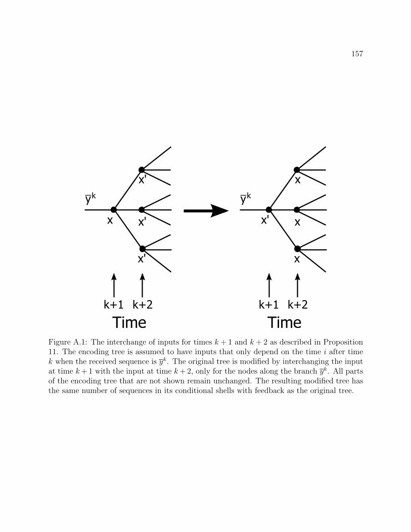
157

Timek+1 k+2

x

yk

x'

x'

x'

Timek+1 k+2

x'

yk

x

x

x

Figure A.1: The interchange of inputs for times k + 1 and k + 2 as described in Proposition11. The encoding tree is assumed to have inputs that only depend on the time i after timek when the received sequence is yk. The original tree is modified by interchanging the inputat time k+ 1 with the input at time k+ 2, only for the nodes along the branch yk. All partsof the encoding tree that are not shown remain unchanged. The resulting modified tree hasthe same number of sequences in its conditional shells with feedback as the original tree.

158

encoding tree along yn has not changed. So suppose that yk = yk, and let zn = τ(yn), so

nP (x)V (y|x) =n∑i=1

1(xi(m, yi−1) = x, yi = y)

=k∑i=1

1(xi(m, yi−1) = x, yi = y) + 1(xk+1(m, y

k) = x, yk+1 = y)+

1(xk+2(m, yk+1) = x, yk+2 = y) +

n∑i=k+3

1(xi(m, yi−1) = x, yi = y)

(a)=

k∑i=1

1(xi(m, yi−1) = x, yi = y) + 1(xk+1(m, y

k) = x, yk+1 = y)+

1(xk+2(m, yk+1) = x, yk+2 = y) +

n∑i=k+3

1(xi(m, yi−1) = x, yi = y)

(b)=

k∑i=1

1(xi(m, yi−1) = x, yi = y) + 1(xk+1(m, y

k) = x, yk+2 = y)+

1(xk+2(m, yk+1) = x, yk+1 = y) +

n∑i=k+3

1(xi(m, yi−1) = x, yi = y)

=n∑i=1

1(xi(m, zi−1) = x, zi = y),

where in (a) we have used the fact that xi does not change for times other than i = k+1, k+2and in (b), we have interchanged both the xi and yi for i = k+ 1, k+ 2. Hence, zn = τ(yn) ∈BE(P, V ). Hence, τ maps BE(P, V ) into BE(P, V ) for each P ∈ Pn, V ∈ Vn(P ). Therefore,since these are disjoint sets, |BE(P, V )| = |BE(P, V )| for each P ∈ Pn, V ∈ Vn(P ).

A.9.2 Proof of theorem

Theorem 3 of Section 2.5: Fix a δ > 0, R > 0. There exists a finite nFT (W,R, δ) suchthat for any fixed-length code with feedback of length n ≥ nFT (W,R, δ) and rate R withencoding trees for all messages satisfying the fixed type encoding tree condition,

− 1

nlogPe(W ) ≤ Esp(R− δ) + δ.

Proof: For now, assume that the fixed type encoding tree condition holds for all messages

159

in the code with the same P ∈ Pn, so ∀ yn ∈ Yn, P (m, yn) = P . With that in mind,

Pe(W ) =1

|M|∑m∈M

PW (Y n /∈ Dm|M = m)

=1

|M|∑m∈M

∑V ∈Vn(P )

PW (Y n ∈ Dcm ∩B(m,P, V )|M = m)

=1

|M|∑

m∈M(P )

∑V ∈Vn(P )

∑yn∈B(m,P,V )∩Dcm

PW (Y n = yn|M = m)

=∑

V ∈Vn(P )

1

|M|∑m∈M

|Dcm ∩B(m,P, V )| exp (−n [D(V ||W |P ) +H(V |P )])

=∑

V ∈Vn(P )

exp (−n [D(V ||W |P ) +H(V |P ) +R])∑m∈M

|B(m,P, V ) ∩ Dcm|

=∑

V ∈Vn(P )

exp (−n [D(V ||W |P ) +H(V |P ) +R])×[∑m∈M

|B(m,P, V )| − |B(m,P, V ) ∩ Dm|

](a)

≥∑

V ∈Vn(P )

exp (−n [D(V ||W |P ) +H(V |P ) +R])

[(∑m∈M

|B(m,P, V )|

)− |TPV |

]≥

∑V ∈Vn(P )

exp (−n [D(V ||W |P ) +H(V |P ) +R])×[(∑m∈M

|B(m,P, V )|

)− exp(nH(PV ))

],

where (a) follows from Proposition 14. From Proposition 2, we know that |B(m,P, V )| ≥

160

exp(nH(V |P ))/(n+ 1)|X ||Y| for all m ∈M , so for any δ > 0, we have

Pe(W ) ≥∑

V ∈Vn(P )

exp (−n [D(V ||W |P ) +H(V |P ) +R])×[exp

(n

[H(V |P ) +R− |X ||Y|

nlog(n+ 1)

])− exp(nH(PV ))

]≥

∑V ∈Vn(P )

exp

(−n[D(V ||W |P ) +

|X ||Y|n

log(n+ 1)

])×[

1− exp

(−n[R−H(PV ) +H(V |P )− |X ||Y|

nlog(n+ 1)

])]≥

∑V ∈Vn(P ):I(P,V )≤R−δ

exp

(−n[D(V ||W |P ) +

|X ||Y|n

log(n+ 1)

])×[

1− exp

(−n[R−H(PV ) +H(V |P )− |X ||Y|

nlog(n+ 1)

])]≥ exp

(−n[

minV ∈Vn(P ):I(P,V )≤R−δ

D(V ||W |P ) +|X ||Y|n

log(n+ 1) + τ(n, δ, |X |, |Y|)])

,

where

τ(n, δ, |X |, |Y|) , − 1

nlog

(1− exp

(−n[δ − |X ||Y|

nlog(n+ 1)

])).

Note that τ(n, δ, |X |, |Y|)→ 0 as n→∞ and is O(1/n). From Lemma 6, we know that

minV ∈Vn(P ):I(P,V )≤R−δ

D(V ||W |P ) ≤ Esp

(R− δ − 2

|X ||Y|n

log n

)+ κW

|X ||Y|n

+|X ||Y|n

logn

|X |.

Therefore,

− 1

nlogPe(W ) ≤ Esp

(R− δ − 2

|X ||Y|n

log n

)+ κW

|X ||Y|n

+|X ||Y|n

logn

|X |+

|X ||Y|n

log(n+ 1) + τ(n, δ, |X |, |Y|).

Now, the above is true when we assume that the fixed type encoding tree condition holdswith the same P for all messages. Removing the requirement that the condition holds withthe same P for all messages means we need to thin the code before applying the argumentthat got us to the point above. Since there are at most (n+ 1)|X | types P that the conditioncan hold with for each message, we have

161

− 1

nlogPe(W ) ≤ Esp

(R− δ − 2

|X ||Y|n

log n− |X |n

log(n+ 1)

)+|X ||Y|n

logn

|X |+

κ|X ||Y|n

+|X ||Y|n

log(n+ 1) + τ(n, δ, |X |, |Y|) +|X |n

log(n+ 1)

Since log(n)/n→ 0 as n→∞, we have for large enough n depending on δ, R and W that

− 1

nlogPe(W ) ≤ Esp(R− 2δ) + 2δ.

A.10 Limited memory at the encoder means the sphere

packing bound holds

Proposition 5 of Section 2.9: The following relationship between Esp(R) and E ′sp(R)holds for all k ≥ 2 (i.e. all interesting k):

E ′sp(R) = kEsp

(R

k

).

This result is due to Baris Nakiboglu and Giacomo Como [33].Proof: We will show this for the case of k = 2 and argue the rest by induction. First,

let S ′ be the set of test channels V ′ ∈ W ′ of the form

V ′(y1, y2|x1, f2) = V1(y1|x1)V2(y2|f2(y1))

for some V1, V2 ∈ W . So, V ′ is a succession of two possibly different DMCs. Then, forV ′ ∈ S ′ ⊂ W ′,

D(V ′||W ′|P ′) =∑x1,f2

∑y1,y2

P ′(x1, f2)V′(y1, y2|x1, f2) log

V ′(y1, y2|x1, f2)W ′(y1, y2|x1, f2)

=∑x1,f2

∑y1,y2

P ′(x1, f2)V1(y1|x1)V2(y2|f2(y1)) logV1(y1|x1)V2(y2|f2(y1))W (y1|x1)W (y2|f2(y1))

=∑x1,f2

∑y1,y2

P ′(x1, f2)V1(y1|x1)V2(y2|f2(y1)) logV1(y1|x1)W (y1|x1)

+

∑x1,f2

∑y1,y2

P ′(x1, f2)V1(y1|x1)V2(y2|f2(y1)) logV2(y2|f2(y1))W (y2|f2(y1))

.

162

Now, for the first term above,

T1 ,∑x1,f2

∑y1,y2

P ′(x1, f2)V1(y1|x1)V2(y2|f2(y1)) logV1(y1|x1)W (y1|x1)

=∑x1,y1

[∑f2

P ′(x1, f2)∑y2

V2(y2|f2(y1))

]V1(y1|x1) log

V1(y1|x1)W (y1|x1)

(a)=∑x1,y1

[∑f2

P ′(x1, f2)

]V1(y1|x1) log

V1(y1|x1)W (y1|x1)

= D(V1||W |PX1) (A.42)

PX1 ,∑f2

P ′(x1, f2),

where (a) follows because for each fd, y1,∑

y2V (y2|f2(y1)) = 1. Note that PX1 depends only

on P ′. For the second term,

T2 ,∑x1,f2

∑y1,y2

P ′(x1, f2)V1(y1|x1)V2(y2|f2(y1)) logV2(y2|f2(y1))W (y2|f2(y1))

=∑x1,f2

∑y1,y2

∑x2

1(f2(y1) = x2)P′(x1, f2)V1(y1|x1)V2(y2|f2(y1)) log

V2(y2|x2)W (y2|x2)

=∑x2,y2

∑x1,y1,f2:f2(y1)=x2

P ′(x1, f2)V1(y1|x1)

V2(y2|f2(y1)) logV2(y2|x2)W (y2|x2)

=∑x2,y2

PX2(x2)V2(y2|f2(y1)) logV2(y2|x2)W (y2|x2)

= D(V2||W |PX2) (A.43)

PX2(x2) ,∑

x1,y1,f2:f2(y1)=x2

P ′(x1, f2)V1(y1|x1),

where we note that PX2(·) is a distribution because it is nonnegative and sums to 1. Notethat PX2 depends on P ′ and V1 but not on V2. Combining (A.42) and (A.43) yields

D(V ′||W ′|P ′) = D(V1||W |PX1) +D(V2||W |PX2). (A.44)

Now, it is well known [47] that for P ∈ P , V ∈ V ,

I(P, V ) = D(V ||(PV )|P )

= minQ∈Q

D(V ||Q|P ),

163

where the divergence between a conditional distribution V and a distribution Q on Y con-ditioned on P is

D(V ||Q|P ) =∑x,y

P (x)V (y|x) logV (y|x)

Q(y).

With this property in mind,

I(P ′, V ′) = minQ′∈Q′

∑x1,f2,y1,y2

P ′(x1, f2)V1(y1|x1)V2(y2|f2(y1)) logV1(y1|x1)V2(y2|f2(y1))

Q(y1, y2)

≤∑

x1,f2,y1,y2

P ′(x1, f2)V1(y1|x1)V2(y2|f2(y1)) logV1(y1|x1)V2(y2|f2(y1))

(PX1V1)(y1)(PX2V2)(y2)

=∑

x1,f2,y1,y2

P ′(x1, f2)V1(y1|x1)V2(y2|f2(y1)) logV1(y1|x1)

(PX1V1)(y1)+

∑x1,f2,y1,y2

P ′(x1, f2)V1(y1|x1)V2(y2|f2(y1)) logV2(y2|f2(y1))(PX2V2)(y2)

=∑x1,y1

[∑f2,y2

P ′(x1, f2)V2(y2|f2(y1))

]V1(y1|x1) log

V1(y1|x1)(PX1V1)(y1)

+

∑x1,f2,y1,y2

P ′(x1, f2)V1(y1|x1)V2(y2|f2(y1)) logV2(y2|f2(y1))(PX2V2)(y2)

=∑x1,y1

PX1(x1)V1(y1|x1) logV1(y1|x1)

(PX1V1)(y1)+

∑x1,f2,y1,y2

P ′(x1, f2)V1(y1|x1)V2(y2|f2(y1)) logV2(y2|f2(y1))(PX2V2)(y2)

= I(PX1 , V1) +∑

x1,f2,y1,y2

P ′(x1, f2)V1(y1|x1)V2(y2|f2(y1)) logV2(y2|f2(y1))(PX2V2)(y2)

= I(PX1 , V1) +∑y2

∑x2

∑x1,y1,f1:f2(y1)=x2

P ′(x1, f2)V1(y1|x1)

V2(y2|x2) logV2(y2|x2)

(PX2V2)(y2)

= I(PX1 , V1) +∑y2

∑x2

PX2(x2)V2(y2|x2) logV2(y2|x2)

(PX2V2)(y2)

I(P ′, V ′) ≤ I(PX1 , V1) + I(PX2 , V2). (A.45)

164

Using the above bound for V ′ ∈ S ′, we can upper bound E ′sp(R) as

E ′sp(R) = maxP ′∈P ′

minV ′∈W ′:I(P ′,V ′)≤R

D(V ′||W ′|P ′)

≤ maxP ′∈P ′

minV ′∈S′:I(P ′,V ′)≤R

D(V ′||W ′|P ′)

(a)

≤ maxP ′∈P ′

minV ′∈S′:I(PX1

,V1)+I(PX2,V2)≤R

D(V ′||W ′|P ′)

(b)

≤ maxP ′∈P ′

minV ′∈S′:I(PX1

,V1)≤R/2, I(PX2,V2)≤R/2

D(V ′||W ′|P ′) (A.46)

(c)= max

P ′∈P ′min

V ′∈S′:I(PX1,V1)≤R/2, I(PX2

,V2)≤R/2D(V1||W |PX1) +D(V2||W |PX2),

where (a) is due to reducing the set of admissible V ′, (b) follows from (A.45) and (c) followsfrom (A.44). Now, we have

E ′sp(R) ≤ maxP ′∈P ′

minV1,V2:I(PX1

,V1)≤R/2, I(PX2,V2)≤R/2

D(V1||W |PX1) +D(V2||W |PX2)

(d)

≤ maxPX1

,PX2

minV1:I(PX1

,V1)≤R/2D(V1||W |PX1) + min

V2:I(PX2,V2)≤R/2

D(V2||W |PX2)

= 2Esp(R/2),

where (d) follows because while PX2 is induced by P ′ and V1, allowing it to be arbitrary canonly make the max larger.

The above proof can be extended to k symbols as follows. First, note that we neverused anywhere explicitly that the first and second symbol within the supersymbol are fromthe same alphabet, so for example we can have X ′ = X × X k−1 and similarly for Y ′ andW ′. Secondly, the bound from the line above (A.46) to (A.46) does not have to be an R/2,R/2 split in the mutual information. We can just as well require I(PX1 , V1) ≤ R/k andI(PX2 , V2) ≤ (k − 1)R/k. In the end, we would have

E ′sp(R) ≤ Esp,1(R/k) + Esp,2((k − 1)R/k), (A.47)

where Esp,1 denotes the sphere packing bound of the first channel and Esp,2 denotes thesphere packing bound for the second channel. So to prove the proposition by induction,assume that we have shown for all l ≤ k (we have already done the base case of k = 2),

E(l)sp (R) ≤ lEsp(R/l),

where E(l)sp (R) denotes the sphere packing bound of the superchannel composed of l symbols

165

from X . Then, using (A.47),

E(k+1)sp (R) ≤ Esp(R/(k + 1)) + E(k)

sp (kR/(k + 1))

(e)

≤ Esp(R/(k + 1)) + kEsp(R/(k + 1))

= (k + 1)Esp(R/(k + 1)),

where (e) follows from the inductive hypothesis. As for the lower bound that E ′sp(R) ≥kEsp(R/k), it follows obviously from the fact that the codes do not have to use feedback atall, that is P ′ can be a product distribution on X k, in which case the optimization turns intok independent optimizations over test channels. Using the fact that both mutual informationand divergence are convex in the channel V yields the desired lower bound. We only outlinethis portion because we actually only need the upper bound for our purposes.

A.11 Equivalent statements

A.11.1 S-P encoding tree condition implies SP holds with feed-back

Proposition 3 of Section 2.6: If the sphere-packing encoding tree condition holds, thensphere-packing for fixed-length codes with feedback holds.

Proof: Fix a δ > 0, and block code with feedback of rateR and length n ≥ nET,fb(δ, R,W ).If the sphere-packing encoding tree condition holds, we know that for each message encodingtree, there exists a P ∈ Pn, V ∈ Vn(P ) such that (2.26), (2.27) and (2.28) hold. Now, the(P, V ) can be different for different messages, but there are at most (n+ 1)|X ||Y| joint types(P, V ), so there must be at least one (P, V ) such that (2.26), (2.27) and (2.28) hold for atleast |M|/(n+ 1)|X ||Y| of the messages. Fixing this P, V , and letting M′ ⊂M be the set ofmessages for which (2.26), (2.27) and (2.28) hold, we have

Pe(W ) =1

|M|∑m∈M

PW (Y n ∈ Dcm|M = m)

≥ 1

|M|∑m∈M

PW (Y n ∈ B(m,P, V ) ∩ Dcm|M = m)

=1

|M|∑m∈M

|B(m,P, V ) ∩ Dcm| exp(−n(D(V ||W |P ) +H(V |P )))

≥ 1

|M|∑m∈M′

|B(m,P, V ) ∩ Dcm| exp(−n(D(V ||W |P ) +H(V |P )))

= exp(−n(R +D(V ||W |P ) +H(V |P ))∑m∈M′

|B(m,P, V ) ∩ Dcm|. (A.48)

166

At this point, we can use the properties of |B(m,P, V )|, D(V ||W |P ) and I(P, V ) that areprovided by the sphere-packing encoding tree condition.∑m∈M′

|B(m,P, V ) ∩ Dcm| =∑m∈M′

|B(m,P, V )| − |B(m,P, V ) ∩ Dm|

≥∑m∈M′

|B(m,P, V )| − |TPV |

≥∑m∈M′

|B(m,P, V )| − exp(nH(PV ))

≥ |M|(n+ 1)|X ||Y|

exp(n(H(V |P )− δ))− exp(nH(PV ))

= exp

(n

[H(V |P ) +R− |X ||Y|

nlog(n+ 1)− δ

])×[

1− exp

(−n[H(V |P )−H(PV ) +R− δ − |X ||Y|

nlog(n+ 1)

])]= exp

(n

[H(V |P ) +R− |X ||Y|

nlog(n+ 1)− δ

])×[

1− exp

(−n[R− I(P, V )− δ − |X ||Y|

nlog(n+ 1)

])]≥ exp

(n

[H(V |P ) +R− |X ||Y|

nlog(n+ 1)− δ

])×[

1− exp

(−n[2δ − δ − |X ||Y|

nlog(n+ 1)

])]= exp

(n

[H(V |P ) +R− |X ||Y|

nlog(n+ 1)− δ

])×[

1− exp

(−n[δ − |X ||Y|

nlog(n+ 1)

])]≥ 1

2exp

(n

[H(V |P ) +R− |X ||Y|

nlog(n+ 1)− δ

]), (A.49)

where the last line holds for large enough n depending on δ, |X | and |Y|. Plugging theinequality of (A.49) into (A.48) yields that for large enough n,

Pe(W ) ≥ 1

2exp

(−n[D(V ||W |P ) + δ +

|X ||Y|n

log(n+ 1)

])≥ 1

2exp

(−n[Esp(R− 2δ) + δ +

|X ||Y|n

log(n+ 1)

]).

Since δ > 0 can be made arbitrarily small and log(n+ 1)/n→ 0 as n→∞, sphere-packingthen holds with feedback.

167

A.11.2 Intermediate S-P condition and S-P holding with feedbackare equivalent

Proposition 4 of Section 2.6: If SP holds with feedback, then the intermediate SPcondition holds. Conversely, if the intermediate SP condition holds, SP holds with feedback.

Proof: First, assume that SP holds with feedback. Fix a δ > 0 and a block code withfeedback of rate R and length n ≥ nSP,fb(δ, R,W ). Now, because SP holds with feedback,

Pe(W ) ≥ exp (−n(Esp(R− δ) + δ)) .

Expanding the error probability,

Pe(W ) =1

|M|∑m∈M

PW (Y n /∈ Dm|M = m)

=1

|M|∑m∈M

∑P∈Pn,V ∈Vn(P )

PW (Y n ∈ B(m,P, V ) ∩ Dcm|M = m)

(a)=

1

|M|∑m∈M

∑P∈Pn,V ∈Vn(P )

|B(m,P, V ) ∩ Dcm| exp(−n(D(V ||W |P ) +H(V |P )))

=∑

P∈Pn,V ∈Vn(P )

1

|M|∑m∈M

|B(m,P, V ) ∩ Dcm| exp(−n(D(V ||W |P ) +H(V |P )))

=∑

P∈Pn,V ∈Vn(P )

K(P, V )

K(P, V ) ,1

|M|∑m∈M

|B(m,P, V ) ∩ Dcm| exp(−n(D(V ||W |P ) +H(V |P ))), (A.50)

where in the above, (a) follows from Proposition 14. Note that all the steps above areequalities. Hence, we know that∑

P∈Pn,V ∈Vn(P )

K(P, V ) ≥ exp(−n(Esp(R− δ) + δ)).

Since all the K(P, V ) are non-negative, and there are at most (n+1)|X ||Y| joint types of lengthn, it follows by the pigeonhole principle that there is at least one P ∈ Pn and V ∈ Vn(P )

168

such that

K(P, V ) =1

|M|∑m∈M

|B(m,P, V ) ∩ Dcm| exp(−n(D(V ||W |P ) +H(V |P )))

≥ 1

(n+ 1)|X ||Y|exp(−n(Esp(R− δ) + δ))

1

nlogK(P, V ) = −D(V ||W |P )−H(V |P ) +

1

nlog

[1

|M|∑m∈M

|B(m,P, V ) ∩ Dcm|

]

≥ −Esp(R− δ)− δ −|X ||Y|n

log(n+ 1).

Rearranging yields

ζ ,1

nlog

[1

|M|∑m∈M

|B(m,P, V ) ∩ Dcm|

](A.51)

≥ H(V |P )−[Esp(R− δ)−D(V ||W |P ) + δ +

|X ||Y|n

log(n+ 1)

]≥ H(V |P )− [Esp(R− δ)−D(V ||W |P ) + 2δ] (A.52)

for n large enough, as log(n+ 1)/n goes to 0 as n→∞. Now,

1

nlog

[1

|M|∑m∈M

|B(m,P, V ) ∩ Dcm|

]≤ 1

nlog

[1

|M|∑m∈M

|B(m,P, V )|

](b)

≤ 1

nlog

[1

|M|∑m∈M

exp(nH(V |P ))

]= H(V |P ), (A.53)

where (b) comes from Proposition 14. Plugging the inequality of (A.53) into (A.52) impliesthat additionally,

D(V ||W |P ) ≤ Esp(R− δ) + 2δ.

Hence, the intermediate sphere packing condition holds.Now, suppose the intermediate sphere packing condition holds. That is, for n ≥ nSPI,fb(δ, R,W )

there exists a P ∈ Pn, V ∈ Vn(P ) such that (2.30) and (2.31) hold. Then, plugging (2.31)into (A.50) and working backwards through the inequalities gives us that the sphere-packingbound holds with feedback.

169

A.12 Delayed feedback

A.12.1 Error probability bound

Lemma 5 of Section 2.7: Define a channel independent constant

α(T ) ,|X |(2 + |Y|) log(T + 1)

T.

Fix an ε > α(T ). Then, for any block length n = NT (with N ≥ 1) rate R coding systemwith a type 2 encoder,

− 1

NTlogPe(NT, E ,D) ≤ Esp,T (R− ε) + α(T ) + γ(N, T, ε),

where

Esp,T (R) , maxP∈PT

minV ∈VT (P ):I(P,V )≤R

D(V ||W |P ), (A.54)

and

γ(N, T, ε) =1

NTlog

1

1− exp(−NT (ε− α(T ))).

Proof: The argument begins, as with the sphere-packing proof for codes without feed-back, by showing that there is a subcode of approximate rate R for which most codewordshave the same input types. This is normally done by whittling down the messages to thosewhose codewords belong to the largest common type, by message population. The challengeis that now we have feedback every T symbols, so we need to carefully show in what sensemessages have the same input types. We do this by induction on N , the total number ofT -length blocks.

First, for N = 1, there has been no feedback. Let P1(m) denote the type of xT (m) ,(φ1(m), . . . , φT (m)). Now, group messages according to their type P1(m). Since |PT | is atmost (T + 1)|X |, there exists a P1 ∈ PT such that

|m : P1(m) = P1| ≥2nR

(T + 1)|X |.

This is the usual argument for fixing the composition of a high-rate subcode in the proof of thesphere-packing bound for codes used without feedback. After this, we choose a V1 ∈ VT (P1)such that I(P1, V1) ≤ R − ε. The choice of V1 is made so as to minimize D(V1||W |P1)amongst those V1 ∈ VT (P1) that have I(P1, V1) ≤ R − ε. The existence of a V1 such thatI(P1, V1) ≤ R − ε is not immediately obvious for channels in which Esp(R) can be infinite,even if Esp(R) is not infinite for the given R. If no such V1 exists, the result of the lemma

170

is meaningless if we take the convention that min over the null set is ∞. Hence, if theoptimization in the right hand side of (2.32) evaluates to something finite, we can safelyassume the existence, for each P1, of a V1 with I(P1, V1) ≤ R− ε. For the rest of the proof,we assume we are in this case.

Without feedback, the selection at this point would be enough to show that for a high-ratesubcode with the same type, a substantial portion of the selected V1-shells (as defined in [47])around the codewords for these messages overlap to cause a significant error. However, wenow have feedback every T symbols, so we will iterate this selection process N times. Wewill prove a claim showing that the messages are not thinned too much and there are manyyn sequences which must ‘overlap’. We will do this by selecting N input types P1, . . . , PNand N channel shells V1, . . . , VN sequentially by induction. Let, for 1 ≤ k ≤ N ,

B(k)(m) ,

ykT :

y(k−1)T ∈ B(k−1)(m), Pk(m, y(k−1)T ) = Pk,

ykT(k−1)T+1 ∈ TVk(xkT(k−1)T+1(m, y

(k−1)T ))

,

where Pk(m, y(k−1)T ) is the type of xkT(k−1)T+1(m, y

(k−1)T ), which is itself defined as(φ(k−1)T+1(m, y

(k−1)T ), . . . , φkT (m, y(k−1)T )).

Now, let for 1 ≤ k ≤ N ,

A(k) ,

m : |B(k)(m)| ≥ exp2(T

∑ki=1H(Vi|Pi))

(T + 1)k(|X |+|X ||Y|)

,

where H(V |p) =∑

x,y p(x)V (y|x) log(1/V (y|x)) denotes conditional entropy. Note the de-

pendence of both the A(k) and B(k)(m) sets on Pi and Vi. We drop the dependence in thenotation for convenience. In words, we are breaking the transmission length into blocks oflength T , and then coming up with a set of messages that have common types within eachblock as long as the output sequence being fed back lies exactly in a certain V-shell. Theset B(k)(m) keeps track of how many of these output sequences lead to the common typefor each message and the set A(k) keeps track of how many of the messages have the desiredlower bound on size for B(k)(m).

Claim 3. For a block length n = NT , rate R type 2 encoder, there exist P1, . . . , PN ∈ PTand V1, . . . , VN , with Vi ∈ arg minV ∈VT (Pi):I(Pi,V )≤R−εD(V ||W |Pi) such that

|A(N)| ≥ 2nR

(T + 1)N |X |.

Proof: We proceed by induction with the base case of N = k = 1. As we have seen thereis a P1 ∈ PT such that at least 2nR/(T + 1)|X | messages have P1(m) = P1. We then chooseV1 ∈ VT (P1) such that I(P1, V1) ≤ R− ε. It is clear that for those m with P1(m) = P1,

|B(1)(m)| = |TV1(P1)| ≥1

(T + 1)|X ||Y|exp2(TH(V1|P1)),

171

where |TV (p)| denotes the number of vectors in a V -shell around a vector of type p (i.e.|TV (xT )| if xT is of type p). Hence, the claim is true for N = 1.

Now for N = k > 1, assume the claim is true for k − 1. For each m ∈ A(k−1), groupthe y(k−1)T ∈ B(k−1)(m) according to Pk(m, y

(k−1)T ). At least |B(k−1)(m)|/(T + 1)|X | of they(k−1)T ∈ B(k−1)(m) have a common type Pk(m, y

(k−1)T ) = Pk(m). Now, group the messagesin A(k−1) according to Pk(m). At least |A(k−1)|/(T + 1)|X | have a common type Pk(m) = Pk.Now select a Vk ∈ VT (Pk) such that I(Pk, Vk) ≤ R − ε. It is now readily seen that for them ∈ A(k−1) with Pk(m) = Pk,

|B(k)(m)| ≥ |B(k−1)(m)|

(T + 1)|X ||TVk(Pk)|

≥exp2

(T∑k

i=1H(Vi|Pi))

(T + 1)k(|X |+|X ||Y|).

This holds for at least |A(k−1)|/(T + 1)|X | ≥ 2nR/(T + 1)k|X | messages, hence the claim istrue.

Now, note that for all yn ∈ B(N)(m) with m ∈ A(N), we also have yiT(i−1)T+1 ∈ TPiVi for all1 ≤ i ≤ N . Hence,

∀ m, B(N)(m) ⊂ TP1V1 × · · · × TPNVN∴ | ∪m∈A(N) B(N)(m)| ≤ |TP1V1| × · · · × |TPNVN |

≤ exp2

(T

N∑i=1

H(PiVi)

), (A.55)

where H(PV ) is the entropy of the distribution (PV )(y) =∑

x p(x)V (y|x). Focusing ourattention on these output sequences,

Pe(n, E ,D) =1

2nR

2nR∑m=1

∑yn /∈ψ−1(m)

n∏i=1

W

(yi

∣∣∣∣φi (m, ybi/T cT ))≥ 1

2nR

∑m∈A(N)

∑yn∈ψ−1(m)∩B(N)(m)

PW (yn|M = m)

(a)=

exp2

(−T

∑Ni=1(D(Vi||W |Pi) +H(Vi|Pi))

)2nR

∑m∈A(N)

|ψ−1(m) ∩B(N)(m)|

=exp2

(−T

∑Ni=1(D(Vi||W |Pi) +H(Vi|Pi))

)2nR

×∑m∈A(N)

(|B(N)(m)| − |B(N)(m) ∩ ψ−1(m)|),

172

where in (a), we have noted that the probability for all yn ∈ B(N)(m) is equal to

exp2

(−T

N∑i=1

(D(Vi||W |Pi) +H(Vi|Pi))

).

Continuing, we have

Pe(n, E ,D) ≥exp2

(−T

∑Ni=1(D(Vi||W |Pi) +H(Vi|Pi))

)2nR

× ∑m∈A(N)

|B(N)(m)|

−∣∣∣∣∣∣⋃

m∈A(N)

B(N)(m)

∣∣∣∣∣∣

≥exp2

(−T

∑Ni=1(D(Vi||W |Pi) +H(Vi|Pi))

)2nR

× |A(N)|2T∑Ni=1H(Vi|Pi)

(T + 1)N(|X |+|X ||Y|) −

∣∣∣∣∣∣⋃

m∈A(N)

B(N)(m)

∣∣∣∣∣∣

(b)

≥ exp2(−T∑N

i=1D(Vi||W |Pi))2nR

[|A(N)|

(T + 1)N(|X |+|X ||Y|) − exp2

(T

N∑i=1

I(Pi, Vi)

)](c)

≥ exp2(−TN∑i=1

D(Vi||W |Pi))[

1

(T + 1)N(2+|Y|)|X | − exp2 (−NTε)]

=exp2

(−T

∑Ni=1D(Vi||W |Pi)

)exp2(NTα(T ))

[1− 2−NT (ε−α(T ))

].

In inequality (b), we have used the inequality of equation (A.55). Claim 3 is used ininequality (c). In the selection process of the claim, for each Pi ∈ PT , we choose a Vi ∈ VT (p)with I(Pi, Vi) ≤ R − ε that minimizes the average divergence. Then, since we can’t sayanything about the Pi, we bound by the worst-case P to take a max over all P ∈ PT . Takinglogs and dividing by NT gives the result of the lemma.

A.12.2 Length T sphere-packing exponent

Lemma 6 of Section 2.7: For any T ≥ 2|X ||Y|, for all P ∈ PT ,

minU∈VT (P ):I(P,U)≤R

D(U ||W |P ) ≤ Esp

(R− 2|X ||Y| log T

T, P

)+κW |X ||Y|

T+

|X ||Y| log(T/|X |)T

,

173

where

Esp(R,P ) , minV :I(P,V )≤R

D(V ||W |P ),

κW , maxx,y:W (y|x)>0

log1

W (y|x).

Proof: First, write P ∈ PT as P (x) = kx/T where kx are nonnegative integers that sumto T .

Claim 4. Let U be an arbitrary channel for which |U(y|x)−V (y|x)| ≤ 1/kx for all x, y, andU(y|x) = V (y|x) = 0 when W (y|x) = 0. Then,

|D(U ||W |P )−D(V ||W |P )| ≤ |X ||Y|κW + log(T/|X |)T

.

Proof: First, note that |r log r− s log s| ≤ −|r− s| log |r− s| whenever r, s ∈ [0, 1]. Thiscan be seen by noting that the function f(r) = −r log r, r ∈ [0, 1] is concave and maximalabsolute slope at r = 0, where the derivative is unbounded above. Hence, |f(r) − f(0)| =−r log r, r ∈ [0, 1] is a bound to the difference between two points on the curve at distancer. Now, keeping in mind that U(y|x) = V (y|x) = 0 whenever W (y|x) = 0, a little algebrashows that

|D(U ||W |P )−D(V ||W |P )| ≤∑x

P (x)∑y

∣∣∣∣U(y|x) logU(y|x)

W (y|x)− V (y|x) log

V (y|x)

W (y|x)

∣∣∣∣≤∑x

kxT

∑y

|U(y|x) logU(y|x)− V (y|x) log V (y|x)|+

∑x

kxT

∑y:W (y|x)>0

|U(y|x)− V (y|x)| log1

W (y|x)

≤∑x

kxT

∑y

[1

kxlog kx +

1

kxκW

]≤ |X ||Y|κW

T+|Y|T

∑x

log kx

(a)

≤ |X ||Y|κWT

+|X ||Y| log T/|X |

T.

In (a), we are also using the fact that since log is a symmetric, concave (∩) function, so

maxkx∈N:

∑x kx=T

∑x

log kx ≤ |X | logT

|X |.

174

Now, for an ε > 0, pick V to be in arg minV ′:I(P,V ′)≤R−εD(V ′||W |P ). We will find aU ∈ VT (P ) such that I(P,U) ≤ I(P, V ) + ε ≤ R. First, we show that there exists aU ∈ VT (P ) such that |U(y|x)− V (y|x)| ≤ 1

kxfor all x, y.

For each x, y, let U(y|x) = bkxV (y|x)c/kx. Note that U is missing some mass to be atransition matrix if the entries of V (·|x) are not multiples of 1/kx. The missing mass can bebounded, for a fixed x,

1−∑y

U(y|x) =∑y

V (y|x)− U(y|x)

≤ |y : kxV (y|x) /∈ Z|/kx.

Now, the missing mass must be a multiple of 1/kx for each x because U(·|x) has terms thatare multiples of 1/kx. Therefore, the missing mass can be distributed amongst the y thathave kxV (y|x) /∈ Z in multiples of 1/kx in such a way so that no y has more than 1/kx mass

added to it. We let U(y|x) be the resulting transition matrix. Since U(y|x) = bkxV (y|x)c/kxand either 0 or 1/kx is added to get to U(y|x), it follows that |V (y|x) − U(y|x)| ≤ 1/kx.Also, U(y|x) = 0 when V (y|x) = 0.

Note that ∑x

p(x)∑y

|U(y|x)− V (y|x)| ≤∑x

kxT

∑y

1

kx≤ |X ||Y|

T.

If T ≥ 2|X ||Y|, we can use the continuity lemma for entropy (Lemma 20). By using thislemma twice after expanding mutual information, we get

|I(P,U)− I(P, V )| ≤ |H(PU)−H(PV )|+ |H(P,U)−H(P, V )|

≤ 2|X ||Y|T

log T.

Hence,

I(P,U) ≤ R− ε+2|X ||Y|T

log T ≤ R

provided

2|X ||Y|T

log T ≤ ε.

Therefore, there exists a U ∈ VT (P ), with I(P,U) ≤ R such that

D(U ||W |P ) = Esp(R− ε, P ) +D(U ||W |P )−D(V ||W |P )

≤ Esp

(R− 2|X ||Y|

Tlog T, P

)+κW |X ||Y|

T+|X ||Y|T

logT

|X |.

175

A.13 The Haroutunian exponent of a parallel channel

Lemma 7 of Section 2.8: Fix a W ∈ W and integer L ≥ 1. Let W (L) denote theprobability transition matrix from X L to YL obtained by using L independent copies of W .That is, for (x1, . . . , xL) = xL ∈ X L and (y1, . . . , yL) = yL ∈ YL,

W (L)(yL|xL) =L∏i=1

W (yi|xi).

Let Eh(LR;W (L)) denote the Haroutunian exponent for W (L) at rate LR and let Esp(R;W )denote the sphere-packing exponent for W at rate R. Then,

Eh(LR;W (L)) ≤ LEsp

(R− |X |

Llog(L+ 1);W

).

Proof: First note that C(W (L)) = LC(W ) because the copies of W in W (L) are independent.Let W(L) denote the set of probability transition matrices from X L to YL. Then,

Eh(LR;W (L)) = minV ∈W(L):C(V )≤LR

maxxL

D(V (·|xL)||W (L)(·|xL)). (A.56)

For each length L type P ∈ PL, fix εL = |X |L

log(L+ 1) and

UP ∈ arg minV ′∈W:I(P,V ′)≤R−εL

D(V ′||W |P ). (A.57)

Then, for each xL ∈ TP , yL ∈ YL, define

V (yL|xL) =L∏i=1

UP (yi|xi). (A.58)

V is a legitimate probability transition matrix in W(L) because it is clearly nonnegative andfor each fixed xL ∈ X L, ∑

yL

V (yL|xL) =∑yL

L∏i=1

UP (yi|xi)

=∑y1

· · ·∑yL

L∏i=1

UP (yi|xi)

=L∏i=1

∑yi∈Y

UP (yi|xi)

=L∏i=1

1 = 1,

176

where P is the type of xL. It is shown in Proposition 12 that C(V ) ≤ LR. Therefore, V isincluded in the minimization for Eh(LR;W (L)). Now, fix an xL and let P be the type of xL,so xL ∈ TP . Then,

D(V (·|xL)||W (L)(·|xL)) =∑yL

V (yL|xL) logV (yL|xL)

W (L)(yL|xL)

=∑yL

[L∏i=1

UP (yi|xi)

]log

∏Lj=1 UP (yj|xj)∏Lj=1W (yj|xj)

=∑yL

[L∏i=1

UP (yi|xi)

][L∑j=1

logUP (yj|xj)W (yj|xj)

]

=L∑j=1

∑yL

[L∏i=1

UP (yi|xi)

]log

UP (yj|xj)W (yj|xj)

=L∑j=1

(∑yi,i 6=j

[∏i 6=j

UP (yi|xi)

])∑yj

UP (yj|xj) logUP (yj|xj)W (yj|xj)

=L∑j=1

(∑yi,i 6=j

[∏i 6=j

UP (yi|xi)

])D(UP (·|xj)||W (·|xj))

(a)=

L∑j=1

D(UP (·|xj)||W (·|xj))

(b)= LD(UP ||W |P )

(c)

≤ LEsp(R− εL;W ),

where (a) follows because the term that disappears is 1, (b) follows because the type of xL

is P and (c) follows by the choice of UP as a sphere-packing optimizing channel in (A.57).This upper bound is independent of xL, therefore

maxxL

D(V (·|xL)||W (L)(·|xL)) ≤ LEsp(R− εL;W ),

which proves the lemma because V is included in the minimization of (A.56).

Proposition 12. For the channel V defined in (A.57) and (A.58), C(V ) ≤ LR.

Proof: Note that by definition17, C(V ) = maxP (L)(XL) I(XL;Y L) where P (L)(XL) is a

probability mass function on X L and P(Y L|XL) = V (Y L|XL). Let Z be the random variable

17Recall that in our notation capital letters such as XL denote random variables.

177

which takes values in PL which takes the value of the type of XL. That is, if XL ∈ TP , Z = P .Note that Z is a deterministic function of XL. Now, for any distribution P (L)(XL),

I(XL, Z;Y L) = I(XL;Y L) + I(Z;Y L|XL)

= I(XL;Y L),

where the first equality follows by chain rule for mutual information and the second equalityfollows because Z is a function of XL and therefore independent of Y L given XL. Now, ifwe expand the other way,

I(XL, Z;Y L) = I(Z;Y L) + I(XL;Y L|Z)

≤ H(Z) + I(XL;Y L|Z)

≤ |X | log(L+ 1) + I(XL;Y L|Z),

where the last line follows by the fact that Z takes its values in the set of types and |PL| ≤(L+ 1)|X |. By definition,

I(XL;Y L|Z) =∑P∈PL

P(Z = P )I(XL;Y L|Z = P )

I(XL;Y L|Z = P ) = H(Y L|Z = P )−H(Y L|Z = P,XL).

Now, because Z = P specifies that XL ∈ TP ,

H(Y L|Z = P,XL) =∑xL∈TP

P(XL = xL|Z = P )H(Y L|XL = xL, Z = P ).

178

For any xL ∈ TP , because we have the Markov property Z −XL − Y L,

H(Y L|XL = xL, Z = P ) =∑yL

V (yL|xL) log1

V (yL|xL)

(a)=∑yL

[L∏i=1

UP (yi|xi)

]log

1∏Lj=1 UP (yj|xj)

=∑yL

[L∏i=1

UP (yi|xi)

][L∑j=1

log1

UP (yj|xj)

]

(b)=

L∑j=1

∑yL

[L∏i=1

UP (yi|xi)

]log

1

UP (yj|xj)

=L∑j=1

∑yj

[UP (yj|xj) log

1

UP (yj|xj)

] ∑yi,i 6=j

∏i 6=j

UP (yi|xi)

=L∑j=1

∑y

[UP (yj|xj) log

1

UP (yj|xj)

](c)= L

∑x

P (x)∑y

UP (y|x) log1

UP (y|x)

= LH(UP |P ),

where (a) follows by the definition of V for xL ∈ TP , (b) follows by the interchange of sumsand products, and (c) follows by the fact that xL ∈ TP and yj is just a dummy variable fory ∈ Y . Now, by chain rule for entropy,

H(Y L|Z = P ) =L∑i=1

H(Yi|Z = P, Y1, . . . , Yi−1)

≤L∑i=1

H(Yi|Z = P )

because conditioning can only reduce entropy. For this fixed P , let Pi be the distribution ofXi conditioned on Z = P . That is Pi(x) = P(Xi = x|Z = P ). Because we have conditioned

179

Z = P , it follows that 1L

∑Li=1 Pi = P . Now, by the Markov property Z −Xi − Yi,

H(Yi|Z = P ) =∑y

P(Yi = y|Z = P ) log1

P(Yi = y|Z = P )

=∑y

[∑x

Pi(x)UP (y|x)

]log

1∑x Pi(x)UP (y|x)

= H(PiUP ).

Hence,

H(Y L|Z = P ) ≤L∑i=1

H(Yi|Z = P )

= LL∑i=1

1

LH(PiUP )

(d)

≤ LH

(1

L

L∑i=1

(PiUP )

)(e)= LH(PUP ),

where (d) follows by concavity (∩) of entropy and (e) follows by linearity and the fact that1L

∑Li=1 Pi = P . Therefore,

I(XL;Y L|Z = P ) = H(Y L|Z = P )−H(Y L|Z = P,XL)

≤ LH(PUP )− LH(UP |P )

= LI(P,UP )

≤ L(R− εL),

where the last inequality follows by the definition of UP in (A.57). Hence, for any distributionP (L) on XL,

I(XL;Y L) ≤ I(XL;Y L|Z) + |X | log(L+ 1)

≤ L(R− εL) + |X | log(L+ 1)

= LR

because LεL = |X | log(L+ 1). Therefore, C(V ) ≤ LR.

A.14 Lemmas for block codes

The lemmas in this appendix are used in results elsewhere in the thesis. They are lemmason typicality as well as continuity of information measures.

180

Lemma 18. Fix a block code of length n, either with or without feedback. Then,

Pe(W ) ≥ Pe(V ) exp(−nd(V,W )),

where

d(V,W ) ,1

|M|∑m∈M

∑yn∈Dcm

PV (Y n = yn|M = m)

Pe(V )

1

n

n∑i=1

logV (yi|xi(m, yi−1))W (yi|xi(m, yi−1))

.

(a) If the code is a block code without feedback and there is a P ∈ Pn such that ∀ m ∈ M,φ(m) ∈ TP , then

d(V,W ) ≤ D(V ||W |P ) +maxκV , κW

Pe(V )β(n, |X |, |Y|),

where

β(n, |X |, |Y|) , infε>0

ε+ (n+ 1)|X ||Y| exp

(−nε

2

2

).

(b) If the code is an arbitrary block code with feedback,

d(V,W ) ≤ maxP

D(V ||W |P ) +maxκV , κW

Pe(V )β(n, |X |, |Y|),

where the constant β(n, |X |, |Y|) is defined above.

Note that by setting ε2 = 2 |X ||Y|+1n

log(n+ 1), we immediately have

β(n, |X |, |Y|) = O

(√log(n)

n

).

Proof: Assume for now that the code has feedback. In the case that it does not (i.e. part(a) of the lemma), we will specialize the result along the way. Also assume thatD(V ||W |P ) <∞ in the non-feedback case and maxP D(V ||W |P ) <∞ in the case with feedback, otherwisethere is nothing to prove.

181

From the definition of Pe(W ), we have

Pe(W ) =1

|M|∑m∈M

PW (Y n ∈ Dcm|M = m)

=1

|M|∑m∈M

∑P∈Pn,U∈Vn(P )

∑yn∈Dcm∩B(m,P,U)

PW (Y n = yn|M = m)

=1

|M|∑m∈M

∑P∈Pn,U∈Vn(P )

∑yn∈Dcm∩B(m,P,U)

PV (Y n = yn|M = m)PW (Y n = yn|M = m)

PV (Y n = yn|M = m)

=1

|M|∑m∈M

∑P∈Pn,U∈Vn(P )

∑yn∈Dcm∩B(m,P,U)

PV (Y n = yn|M = m)n∏i=1

W (yi|xi(m, yi−1))V (yi|xi(m, yi−1))

=1

|M|∑m∈M

∑P∈Pn,U∈Vn(P )

∑yn∈Dcm∩B(m,P,U)

PV (Y n = yn|M = m)∏x,y

[W (y|x)

V (y|x)

]nP (x)U(y|x)

,

where the last line follows from the definition of B(m,P, U). Note that in the above, bythe finite conditional divergence assumptions, if PW (Y n = yn|M = m) = 0, then PV (Y n =yn|M = m) = 0 also. Continuing, and multiplying and dividing by Pe(V ), we have

Pe(W )

Pe(V )≥ 1

|M|∑m∈M

∑P∈Pn,U∈Vn(P )

∑yn∈Dcm∩B(m,P,U)

PV (Y n = yn|M = m)

Pe(V )

∏x,y

[W (y|x)

V (y|x)

]nP (x)U(y|x)

=1

|M|∑m∈M

∑P∈Pn,U∈Vn(P )

∑yn∈Dcm∩B(m,P,U)

PV (Y n = yn|M = m)

Pe(V )×

exp

(−n

[∑x,y

P (x)U(y|x) logV (y|x)

W (y|x)

])(A)

≥ exp

(− n

[1

|M|∑m∈M

∑P∈Pn,U∈Vn(P )

∑yn∈Dcm∩B(m,P,U)

PV (Y n = yn|M = m)

Pe(V )×

∑x,y

P (x)U(y|x) logV (y|x)

W (y|x)

])

= exp

(− n

[1

|M|∑m∈M

∑P∈Pn,U∈Vn(P )

∑yn∈Dcm∩B(m,P,U)

PV (Y n = yn|M = m)

Pe(V )

1

n×

n∑i=1

logV (yi|xi(m, yi−1))W (yi|xi(m, yi−1))

]),

where (A) follows by Jensen’s inequality applied to the function f(t) = et and the last linefollows by the definitive property of yn ∈ B(m,P, U). Fix an ε > 0. We can focus our

182

attention on d(V,W ) by splitting it into two terms,

d(V,W ) =1

|M|∑m∈M

∑P∈Pn,U∈Vn(P )

∑yn∈Dcm∩B(m,P,U)

PV (Y n = yn|M = m)

Pe(V )×

∑x,y

P (x)U(y|x) logV (y|x)

W (y|x)

= T1 + T2

T1 ,1

|M|∑m∈M

∑P∈Pn,U∈Vn(P ):(P,U)∈Jε(V )

∑yn∈Dcm∩B(m,P,U)

PV (Y n = yn|M = m)

Pe(V )×

∑x,y

P (x)U(y|x) logV (y|x)

W (y|x)

T2 ,1

|M|∑m∈M

∑P∈Pn,U∈Vn(P ):(P,U)/∈Jε(V )

∑yn∈Dcm∩B(m,P,U)

PV (Y n = yn|M = m)

Pe(V )×

∑x,y

P (x)U(y|x) logV (y|x)

W (y|x),

where

Jε(V ) =

(P,U) ∈ P ×W :

∑x,y

P (x)|U(y|x)− V (y|x)| ≤ ε

.

For the (P,U) ∈ Jε(V ) in T1, Proposition 13 tells us that∑x,y

P (x)U(y|x) logV (y|x)

W (y|x)≤ D(V ||W |P ) + εmaxκV , κW.

For T2, Lemma 19 tells us that for all m ∈M,∑P∈Pn,U∈Vn(P ):(P,U)/∈Jε(V )

PV (Y n ∈ B(m,P, U)|M = m) ≤ (n+ 1)|X ||Y| exp

(−nε

2

2

). (A.59)

Now, if W (y|x) = 0, and U(y|x) > 0 for some yn in the sum for T2, then we are alsoguaranteed that PV (Y n = yn|M = m) = 0, so that yn does not change the sum. Hence, forall yn that have non-zero terms in the sum for T2,∑

x,y

P (x)U(y|x) logV (y|x)

W (y|x)≤ κW .

183

So, we have

T1 ≤1

|M|∑m∈M

∑P∈Pn,U∈Vn(P ):(P,U)∈Jε(V )

∑yn∈Dcm∩B(m,P,U)

PV (Y n = yn|M = m)

Pe(V )×

[D(V ||W |P ) + εmaxκV , κW] (A.60)

T2 ≤κWPe(V )

1

|M|∑m∈M

∑P∈Pn,U∈Vn(P ):(P,U)/∈Jε(V )

PV (Y n ∈ B(m,P, U) ∩ Dcm|M = m)

≤ κWPe(V )

1

|M|∑m∈M

∑P∈Pn,U∈Vn(P ):(P,U)/∈Jε(V )

PV (Y n ∈ B(m,P, U)|M = m)

≤ κWPe(V )

(n+ 1)|X ||Y| exp

(−nε

2

2

),

where the last line follows from averaging over the bound in (A.59), which holds uniformlyfor all m ∈ M. Now, if the code does not have feedback and all codewords have type P asis assumed in part (a) of the lemma, then

T1 ≤ [D(V ||W |P ) + εmaxκV , κW]×1

|M|∑m∈M

∑U∈Vn(P ):(P,U)∈Jε(V )

PV (Y n ∈ Dcm ∩B(m,P, U)|M = m)

Pe(V )

≤ [D(V ||W |P ) + εmaxκV , κW]1

|M|∑m∈M

∑U∈Vn(P )

PV (Y n ∈ Dcm ∩B(m,P, U)|M = m)

Pe(V )

= [D(V ||W |P ) + εmaxκV , κW]1

|M|PV (Y n ∈ Dcm|M = m)

Pe(V )

= [D(V ||W |P ) + εmaxκV , κW].

Therefore, for part (a) of the lemma,

d(V,W ) ≤ T1 + T2

≤ [D(V ||W |P ) + εmaxκV , κW] +κWPe(V )

(n+ 1)|X ||Y| exp

(−nε

2

2

)≤ D(V ||W |P ) +

maxκV , κWPe(V )

[ε+ (n+ 1)|X ||Y| exp

(−nε

2

2

)].

Optimizing over ε > 0 gives the result of part (a) of the lemma. As for part (b), if the code

184

does have feedback, we can continue bounding T1 in (A.60) below to get

T1 ≤1

|M|∑m∈M

∑P∈Pn,U∈Vn(P ):(P,U)∈Jε(V )

∑yn∈Dcm∩B(m,P,U)

PV (Y n = yn|M = m)

Pe(V )×

[D(V ||W |P ) + εmaxκV , κW]

≤[maxP∈P

D(V ||W |P ) + εmaxκV , κW]×

1

|M|∑m∈M

∑P∈Pn,U∈Vn(P ):(P,U)∈Jε(V )

PV (Y n ∈ B(m,P, U) ∩ Dcm|M = m)

Pe(V )

≤[maxP∈P

D(V ||W |P ) + εmaxκV , κW]×

1

|M|∑m∈M

∑P∈Pn,U∈Vn(P )

PV (Y n ∈ B(m,P, U) ∩ Dcm|M = m)

Pe(V )

=

[maxP∈P

D(V ||W |P ) + εmaxκV , κW]

1

|M|∑m∈M

PV (Y n ∈ ∩Dcm|M = m)

Pe(V )

=

[maxP∈P

D(V ||W |P ) + εmaxκV , κW].

Combining this with the bound on T2, we have for part (b),

d(V,W ) ≤ T1 + T2

≤[maxP∈P

D(V ||W |P ) + εmaxκV , κW]

+κWPe(V )

(n+ 1)|X ||Y| exp

(−nε

2

2

)≤ max

P∈PD(V ||W |P ) +

maxκV , κWPe(V )

[ε+ (n+ 1)|X ||Y| exp

(−nε

2

2

)].

Once again, optimizing over ε > 0 gives the result of part (b).

Lemma 19. Fix an ε > 0 and a block code of length n either with or without feedback. Fora given m ∈M, V ∈ W, define the typical set under channel V ,

Am,ε(V ) , yn : (P (m, yn), V (m, yn)) ∈ Jε(V ) ,

where

Jε(V ) ,

(P,U) ∈ P ×W :

∑x∈X

P (x)∑y∈Y

|U(y|x)− V (y|x)| ≤ ε

.

185

Then,

PV (Y n /∈ Am,ε(V )|M = m) ≤ (n+ 1)|X ||Y| exp

(−nε

2

2

).

Note that for a block code that does not have feedback, if xn(m) ∈ TP for some type P ∈ Pn,

Am,ε(V ) = yn : yn ∈ TU(xn(m)), U ∈ Vn(P ), (P,U) ∈ Jε(V ) .

Proof: For now, assume that the code has feedback. Any code without feedback can bethought of as having feedback and not using it.

For a (P,U) /∈ Jε(V ),

D(U ||V |P )(a)=∑x

P (x)D(U(·|x)||V (·|x))

(b)

≥∑x

P (x)1

2

(∑y

|U(y|x)− V (y|x)|

)2

(c)

≥ 1

2

(∑x

P (x)∑y

|U(y|x)− V (y|x)|

)2

(d)

≥ ε2

2.

In the above, (a) follows by the definition of conditional divergence, (b) follows by Pinsker’sinequality [47], (c) from an application of Jensen’s inequality to the function f(t) = t2 and(d) follows from the assumption that (P,U) ∈ Jε(V ).

Recall the definition of B(m,P, U) for P ∈ Pn, U ∈ Vn(P ),

B(m,P, U) = yn : P (m, yn) = P, V (m, yn) = U.

Using the fact that there are no more than (n+ 1)|X ||Y| joint types (P,U), we have

PV (Y n /∈ Am,ε(V )|M = m) =∑

(P,U)/∈Jε(V )

PV (Y n ∈ B(m,P, U)|M = m)

(a)

≤∑

(P,U)/∈Jε(V )

exp(−nD(V ||W |P ))

≤ (n+ 1)|X ||Y| exp

(−nε

2

2

),

where (a) follows by Proposition 14.For a block code without feedback, it is clear that yn ∈ B(m,P, U) if and only if yn ∈

TU(xn(m)), hence

Am,ε(V ) = yn : yn ∈ TU(xn(m)), U ∈ Vn(P ), (P,U) ∈ Jε(V ) .

186

Proposition 13. Let P ∈ P , U, V,W ∈ W and recall that κV = maxx,y:V (y|x)>0 log 1/V (y|x)(similarly for κW ). Assume that V (y|x) = U(y|x) = 0 whenever W (y|x) = 0. If for someε > 0, (P,U) ∈ Jε(V ), that is,∑

x

P (x)∑y

|U(y|x)− V (y|x)| ≤ ε,

then ∑x

P (x)∑y

U(y|x) logV (y|x)

W (y|x)≤ D(V ||W |P ) + εmax κV , κW .

Proof: Forgive the excessively slow pace of this proof, but several times I thought thatI had proved that the discrepancy from D(V ||W |P ) was bounded by κW ε, when that is notthe case. First,∑x

P (x)∑y

U(y|x) logV (y|x)

W (y|x)=∑x

P (x)∑y

V (y|x) logV (y|x)

W (y|x)+

∑x

P (x)∑y

(U(y|x)− V (y|x)) logV (y|x)

W (y|x)

= D(V ||W |P ) +∑x

P (x)∑y

(U(y|x)− V (y|x)) logV (y|x)

W (y|x).

187

Now, splitting the ‘extra’ term above into different cases yields

T ,∑x

P (x)∑y

(U(y|x)− V (y|x)) logV (y|x)

W (y|x)

=∑

x,y:U(y|x)>V (y|x)

P (x)(U(y|x)− V (y|x)) logV (y|x)

W (y|x)+

∑x,y:U(y|x)<V (y|x)

P (x)(U(y|x)− V (y|x)) logV (y|x)

W (y|x)

(a)

≤∑

x,y:U(y|x)>V (y|x)

P (x)(U(y|x)− V (y|x))κW+

∑x,y:U(y|x)<V (y|x)

P (x)(U(y|x)− V (y|x)) logV (y|x)

W (y|x)

=∑

x,y:U(y|x)>V (y|x)

P (x)(U(y|x)− V (y|x))κW+

∑x,y:U(y|x)<V (y|x)<W (y|x)

P (x)(U(y|x)− V (y|x)) logV (y|x)

W (y|x)+

∑x,y:U(y|x)<V (y|x),W (y|x)<V (y|x)

P (x)(U(y|x)− V (y|x)) logV (y|x)

W (y|x)

=∑

x,y:U(y|x)>V (y|x)

P (x)(U(y|x)− V (y|x))κW+

∑x,y:U(y|x)<V (y|x)<W (y|x)

P (x)(V (y|x)− U(y|x)) logW (y|x)

V (y|x)+

∑x,y:U(y|x)<V (y|x),W (y|x)<V (y|x)

P (x)(V (y|x)− U(y|x)) logW (y|x)

V (y|x)

≤∑

x,y:U(y|x)>V (y|x)

P (x)(U(y|x)− V (y|x))κW+

∑x,y:U(y|x)<V (y|x)<W (y|x)

P (x)(V (y|x)− U(y|x))κV +

∑x,y:U(y|x)<V (y|x),W (y|x)<V (y|x)

P (x)(V (y|x)− U(y|x))0

≤∑x,y

P (x)|U(y|x)− V (y|x)|max κW , κV

≤ εmax κW , κV ,

188

where (a) follows because V (y|x) ≤ 1 and log 1/W (y|x) ≤ κW for the x, y where (U(y|x)−V (y|x)) 6= 0. Similar reasoning yields the other inequalities above.

Proposition 14. For a fixed blocklength code with feedback, for each message m and P ∈ Pn,V ∈ Vn(P ), recall the ’conditional shell with feedback’

B(m,P, V ) , yn : P (m, yn) = P, V (m, yn) = V .Some properties of B(m,P, V ) are

(a) B(m,P, V ) ⊂ TPV ⊂ Yn

(b) If yn ∈ B(m,P, V ),

PW (Y n = yn|M = m) = exp (−n [D(V ||W |P ) +H(V |P )])

(c) |B(m,P, V )| ≤ exp(nH(V |P ))

(d) PW (Y n ∈ B(m,P, V )|M = m) ≤ exp(−nD(V ||W |P )).

Proof: Item (a) is true for the same reason that if yn ∈ TV (P ), yn ∈ TPV ⊂ Yn. As for(b), if yn ∈ B(m,P, V ),

PW (Y n = yn|M = m) =n∏i=1

W (yi|xi(m, yi−1))

=∏x,y

W (y|x)∑ni=1 1(xi(m,y

i−1)=x,yi=y)

= exp

(−n

[∑x,y

log1

W (y|x)

1

n

n∑i=1

1(xi(m, yi−1) = x, yi = y)

])

= exp

(−n

[∑x,y

log1

W (y|x)P (x)V (y|x)

])

= exp

(−n

[∑x,y

P (x)V (y|x)

(log

V (y|x)

W (y|x)+ log

1

V (y|x)

)])= exp (−n [D(V ||W |P ) +H(V |P )]) .

To prove (c), we can apply item (b) with the ‘true channel’ being set to V to get a bound asfollows.

1 ≥ PV (Y n ∈ B(m,P, V )|M = m)

=∑

yn∈B(m,P,V )

PV (Y n = yn|M = m)

= |B(m,P, V )| exp(−n[D(V ||V |P ) +H(V |P )])

= |B(m,P, V )| exp(−nH(V |P )).

189

Therefore, |B(m,P, V )| ≤ exp(nH(V |P )). Finally, we can combine (b) and (c) to get (d):

PW (Y n ∈ B(m,P, V )|M = m) =∑

yn∈B(m,P,V )

PW (Y n = yn|M = m)

=∑

yn∈B(m,P,V )

exp (−n [D(V ||W |P ) +H(V |P )])

= |B(m,P, V )| exp (−n [D(V ||W |P ) +H(V |P )])

≤ exp (−nD(V ||W |P )) .

Proposition 15. Suppose P ∈ P and V,W ∈ W with∑

x P (x)∑

y |V (y|x) −W (y|x)| ≤ε ≤ 1/2. Then,

(a) |H(V |P )−H(W |P )| ≤ ε log|X ||Y|ε

(b) |I(P, V )− I(P,W )| ≤ 2ε log|X ||Y|ε

.

Proof: Consider the distribution (P, V ) on X×Y with (P, V )(x, y) = P (x)V (y|x). Then,

|H(V |P )−H(W |P )| = |H(P ) +H(V |P )−H(P )−H(W |P )|= |H(P, V )−H(P,W )|(a)

≤ ε log|X ||Y|ε

.

In the above, (a) follows from Lemma 20 applied to joint distributions (P, V ) and (P,W ),while noting that∑

x,y

|(P, V )(x, y)− (P,W )(x, y)| =∑x

P (x)∑y

|V (y|x)−W (y|x)| ≤ ε.

As for part (b) of the proposition, note that

|I(P, V )− I(P,W )| = |H(PV )−H(V |P )−H(PW ) +H(W |P )|≤ |H(PV )−H(PW )|+ |H(V |P )−H(W |P )|

≤ ε log|Y|ε

+ ε log|X ||Y|ε

≤ 2ε log|X ||Y|ε

,

190

where the bound on |H(PV )−H(PW )| follows from Lemma 20 and noting that

∑y

|(PV )(y)− (PW )(y)| =∑y

∣∣∣∣∣∑x

P (x)(V (y|x)−W (y|x))

∣∣∣∣∣≤∑x

P (x)∑y

|V (y|x)−W (y|x)|

≤ ε.

Lemma 20 (Uniform continuity of entropy, [21], Theorem 16.3.2). Suppose P and P ′ aredistributions on a finite alphabet X and ||P − P ′||1 =

∑x∈X |P (x)− P ′(x)| ≤ 1/2, then

|H(P )−H(P ′)| ≤ ||P − P ′||1 log|X |

||P − P ′||1.

Lemma 21 (Pinsker’s Inequality, [21], Lemma 12.6.1). Suppose P and P ′ are distributionson a finite alphabet X . Then, with all logarithms and exponentials to the base e,

D(P ||P ′) ≥ 1

2

(∑x

|P (x)− P ′(x)|

)2

.

191

Appendix B

Fixed delay coding appendix

B.1 Proof of Theorem 8

We will now rigorously prove Theorem 8 following the outline given in Section 3.6. The goalis to show that for a given rate R > 0,

supC∈CR

E(C) ≤ E(R) = minV :C(V )≤R

maxP :I(P,W )≥R

D(V ||W |P ).

We will show that E(C) ≤ E(R − ε) for all ε > 0, and therefore, E(C) ≤ limε↓0 E(R − ε),provided the limit exists. In Lemma 25, it is shown that E(R) = limε↓0 E(R − ε) for allR > 0, which will complete the proof.

B.1.1 Inducing error by forming a block code

So first, fix an ε ∈ (0, R), a V ∈ W such that C(V ) ≤ R−ε and a C ∈ CR. Fix a d, d ≥ 1. The

required properties of d, d will be described later in the proof. The first step is to constructa random block code of length n ≥ d as shown in Fig. 3.8. The message bits are

M =(B1, . . . , Bb(n−d+1)Rc

).

The encoder randomizes the code using the bits that arrive after time n− d+ 1, that is thecommon randomness is

U =(Bb(n−d+1)Rc+1, . . . , BbnRc

).

The encoder for this block code is the encoder for C. The decoder for this block code is thedelay-d decoder from D applied to all the bits in the message,

M =(B1(d), . . . , Bb(n−d+1)Rc(d)

).

192

The rate of the code is

R =b(n− d+ 1)Rc

n

≥ (n− d+ 1)R− 1

n

= R− (d− 1)R + 1

n.

It follows that R ≥ R− ε/2 if

n ≥⌈

2[(d− 1)R + 1]

ε

⌉. (B.1)

So for n large enough depending on d,R and ε, the rate of the block code is at least R− ε/2.

Definition 12. A rate-R decoder with feedforward information D is set of decodersD =

Di,d

i≥1,d≥1 that have access to both all received channel outputs as well as all the past

message bit realizations. So,

Di,d : 0, 1i−1 × Ydi/Re+d−1 → 0, 1.

Clearly, any regular decoder D is also a feedforward decoder since the feedforward decodercan choose to ignore the past message bits.

For any feedforward decoder, [37] shows that there is a feedforward decoder that usesonly the d recent channel outputs since the bit arrived at the encoder as well as the pastmessage bits, which performs at least as well as the original feedforward decoder for channelW .

Lemma 22. [Lemma 4.1 of [37]] For a memoryless channel, a rate-R encoder E and a rate-

R feedforward decoder D, there is another feedforward decoder Df =Dfi,d

i≥1,d≥0

using

only the past d channel outputs and the past message bits that performs at least as well asD. That is,

Dfi,d : 0, 1i−1 × Yd → 0, 1

Bfi (d) = Dfi,d

(Bi−1, Y

di/Re+d−1di/Re

)PW

(Bi 6= Dfi,d

(Bi−1, Y

di/Re+d−1di/Re

))≤ PW

(Bi 6= Di,d

(Bi−1, Y di/Re+d−1

))≤ PW

(Bi 6= Di,d

(Y di/Re+d−1

)).

The intuition behind this lemma is that if the channel is memoryless, the past message bitsprovide us with more information about the inputs coming after bit i has entered the encoderthan the past channel outputs.

193

Lemma 22 tells us that if we can prove a lower bound to the error probability for theclass of feedforward decoders that use only recent channel outputs, then we can also lowerbound the error probability to our actual decoder. The upshot is that a change-of-measureargument applied to these feedforward decoders using recent channel outputs only requiresthe ‘true’ channel W to act like a ‘test’ channel V for d time units, as opposed to the full nsymbols of the block code.

Define Bfi (d) = Bf

i (d) ⊕ Bi to be the error sequence for decoder Df . Now, Lemmas 4.2and 4.3 of [37] show that, provided n is large enough as in Eqn. (B.1),

H(Bf,b(n−d+1)Rc(d)

)≥ n(R− ε/2)− I(Xn;Y n),

where I(Xn;Y n) denotes the mutual information between the random variables Xn and Y n

(e.g. as in the textbook of Cover and Thomas [21]). It is straightforward to check (it is apart of the converse to the channel coding theorem in [21]) that under a channel V withC(V ) ≤ R− ε,

I(Xn;Y n) ≤ nC(V ) ≤ n(R− ε)

H(Bf,b(n−d+1)Rc(d)

)≥ nε/2.

The sum of the marginal entropies is at least the entropy of all the error bits, so

b(n−d+1)Rc∑i=1

H(Bfi (d)

)≥ nε/2

1

nR

b(n−d+1)Rc∑i=1

H(Bfi (d)

)≥ ε/2R.

Since entropy is non-negative and b(n− d+ 1)Rc ≤ nR, it follows that there is at least one

i such that H(Bfi (d)) ≥ ε/2. Then, for this i, it follows from the monotonicity of the binary

entropy function hb(t) = −t log t− (1− t) log(1− t), t ∈ [0, 1], that

PV(Bi 6= Dfi,d

(Bi−1, Y

di/Re+d−1di/Re

))≥ h−1b

( ε

2R

). (B.2)

For each bi ∈ 0, 1i, denote the error set for Dfi,d to be

A(bi) ,ydi/Re+d−1di/Re ∈ Yd : Dfi,d

(bi−1, y

di/Re+d−1di/Re

)6= bi

.

Combining this definition of the error set with (B.2) gives

h−1b

( ε

2R

)≤

∑bb(di/Re+d−1)Rc∈0,1b(di/Re+d−1)Rc

1

2b(di/Re+d−1)Rc×

PV(A(bi)

∣∣∣Bb(di/Re+d−1)Rc = bb(di/Re+d−1)Rc). (B.3)

194

Define the set G as

G ,bb(di/Re+d−1)Rc : PV

(A(bi)

∣∣∣Bb(di/Re+d−1)Rc = bb(di/Re+d−1)Rc)≥ h−1b

( ε

2R

).

It is easily verified that

P(G) ≥ h−1b

( ε

2R

)as assuming the contraposition leads to a contradiction of (B.3). At this point, we divergefrom the proof in [37]. We will now use the assumption that C is a good anytime code toshow that the type of the input over the d time steps of interest must be able to support arate close to R over the channel W .

B.1.2 The second block code construction

We wish to study the type of the input during the d time steps after bit i arrives at theencoder. In order to do so, we will construct a second randomized block code as shown inFig. 3.9. The length of the block code is d and the message bits are

M =(Bi, . . . , Bb(di/Re+d−d)Rc

).

The rate of the block code is therefore⌊(di/Re+ d− d)R

⌋− i+ 1

d≥ (di/Re+ d− d)R− i

d

≥ R− d

dR.

Fix a γ > 0. The rate of this block code is at least R − γ provided that d ≤ bγd/Rc. Therandomness used at the encoder is

U =(B1, . . . , Bi−1, Bb(di/Re+d−d)Rc+1, . . . , Bb(di/Re+d−1)Rc

),

that is, both the bits that come before i and the ones that arrive at the encoder after timedi/Re + d − d. The decoder used will be the feedforward delay-d decoder that uses pastmessage bits as well as recent channel outputs Df from Lemma 22. So, the decoded messageis

M =

(Bfi (d), . . . , Bf

b(di/Re+d−d)Rc(d)

).

195

Since we have used the feedforward decoder, the performance of this block code, averagedover the randomness in U is bounded by

PW (M 6= M)(A)

≤b(di/Re+d−d)Rc∑

i′=i

PW(Bfi′(d) 6= Bi′

)≤ dR sup

i′PW

(Bfi′(d) 6= Bi′

)≤ dR sup

i′PW

(Bi′(d) 6= Bi′

),

where (A) follows by union bound. By assumption, E(C) ≥ 2E(R)/3, otherwise there is

nothing to prove for this C. Therefore, there is some d0 such that if d ≥ d0(C),

supi′

PW(Bi′(d) ≤ Bi′

)≤ exp(−dE(R)/2).

So for d ≥ d0,

PW (M 6= M) ≤ dR exp(−dE(R)/2) = exp

(−d

[d

2dE(R)− 1

dlog dR

]),

and for d ≥ d1(d/d), log(dR)/d ≤ E(R)d/4d, so

PW (M 6= M) ≤ dR exp(−dE(R)/2) = exp

(−d

[d

4dE(R)

]).

Letting PW (M 6= M |U) denote the error probability conditioned on a value of the commonrandomness, we have by Markov’s inequality that

P

(PW (M 6= M |U) > exp

(d

[d

8dE(R)

])× exp

(−d

[d

4dE(R)

]))≤ exp

(−d

[d

8dE(R)

]).

So for(

1− exp(−d[d8dE(R)

]))fraction of the realizations of U , the error probability of

the deterministic block code for that value of U is at most exp(−d[d8dE(R)

])provided that

d ≥ max(d1(d/d), d0(C)). Let U be the set of u for which the bound

PW (M 6= M |U = u) ≤ exp

(−d

[d

8dE(R)

])

196

holds. For these realizations of the block code, we will apply Lemma 23 with the tuple(n, δ, α,R) in Lemma 23 being the parameters (d, γ, dE(R)/8d,R − γ) here. The lemma

then says that if d is large enough, depending on γ, dE(R)/8d, |X | and |Y|, then

P(

Type of Xdi/Re+d−1di/Re = P, I(P,W ) ≤ R− 2γ

∣∣∣U ∈ U) ≤ exp

(−d[γ

4− |X |

dlog(d+ 1)

]).

Therefore, unconditioned on the common randomness,

P(

Type of Xdi/Re+d−1di/Re = P, I(P,W ) > R− 2γ

)≥ P

(Type of X

di/Re+d−1di/Re = P, I(P,W ) > R− 2γ, U ∈ U

)≥ P

(Type of X

di/Re+d−1di/Re = P, I(P,W ) > R− 2γ|U ∈ U

)×(

1− exp

(−d

[d

8dE(R)

]))

≥(

1− exp

(−d[γ

4− |X |

dlog(d+ 1)

]))×(

1− exp

(−d

[d

8dE(R)

])),

for d and d large enough. Define the set

Gγ ,bb(di/Re+d−1)Rc : Type of x

di/Re+d−1di/Re = P, I(P,W ) > R− 2γ

.

So, we have that

P(Gγ) ≥(

1− exp

(−d[γ

4− |X |

dlog(d+ 1)

]))(1− exp

(−d

[d

8dE(R)

]))

for large enough d and d. Recall the set

G ,bb(di/Re+d−1)Rc : PV

(A(bi)

∣∣∣Bb(di/Re+d−1)Rc = bb(di/Re+d−1)Rc)≥ h−1b

( ε

2R

).

and that

P(G) ≥ h−1b

( ε

2R

).

197

Now,

P(G ∩Gγ) = 1− P(Gc ∪Gcγ)

≥ 1− P(Gc)− P(Gcγ)

≥ 1−(

1− h−1b( ε

2R

))−(

1−(

1− exp

(−d[γ

4− |X |

dlog(d+ 1)

]))(1− exp

(−d

[d

8dE(R)

])))≥ 1

2h−1b

( ε

2R

), (B.4)

where the last line holds for all d larger than some finite d2(ε/2R, C, γ, d/d, d, E(R), |X |, |Y|)since the exponents are all positive in the second to last line above. When we take the limitof d going to infinity, we will particularly need d/d to not decay too fast (i.e. keep it isa small constant, take the limit as d → ∞, and repeat the entire argument for a smallerratio d/d). So, we have succeeded in showing that the type supports a rate near R for largeenough d. At this point, we can finish the proof with a change of measure argument.

B.1.3 Finishing with a change of measure argument

Lemma 24 shows that if an event has a non-vanishing error probability under channel V ,and the type of the input is known to have high mutual information, the probability of theevent under W can be lower bounded with a divergence term that is constrained by theinput distribution. In particular, if bb(di/Re+d−1)Rc ∈ G ∩Gγ, this means that

PW(Bfi (d) 6= Bi

∣∣∣bb(di/Re+d−1)Rc) = PW(Ydi/Re+d−1di/Re ∈ A(bi)

∣∣∣∣bb(di/Re+d−1)Rc)≥ 1

2h−1b

( ε

2R

)× exp

(−d[

maxP :I(P,W )≥R−2γ

D(V ||W |P )+√4|X ||Y|

dlog(d+ 1) maxκV , κW

]),

198

provided that d is larger than some finite number depending on h−1b (ε/2R), |X | and |Y|.Using the above, we have

ζ , PW (Bi(d) 6= Bi)

≥ PW (Bfi (d) 6= Bi)

=∑

bb(di/Re+d−1)Rc

P(bb(di/Re+d−1)Rc

)PW

(Ydi/Re+d−1di/Re ∈ A(bi)

∣∣∣∣bb(di/Re+d−1)Rc)≥

∑bb(di/Re+d−1)Rc∈G∩Gγ

P(bb(di/Re+d−1)Rc

)PW

(Ydi/Re+d−1di/Re ∈ A(bi)

∣∣∣∣bb(di/Re+d−1)Rc)≥ 1

2h−1b

( ε

2R

) ∑bb(di/Re+d−1)Rc∈G∩Gγ

P(bb(di/Re+d−1)Rc

)×

exp

(−d

[max

P :I(P,W )≥R−2γD(V ||W |P ) +

√4|X ||Y|

dlog(d+ 1) maxκV , κW

])

≥ 1

4h−1b

( ε

2R

)2exp

(−d[

maxP :I(P,W )≥R−2γ

D(V ||W |P )+√4|X ||Y|

dlog(d+ 1) maxκV , κW

]).

Now, if we let γ ≤ minε/2, and let d and d tend to∞ while the ratio d/d is at most γ (whilenot being much smaller, up to integer effects), we can take log and the limit as d → ∞ toget

lim supd→∞

−1

dlogPe(d, C) ≤ max

P :I(P,W )≥R−εD(V ||W |P ).

If V is an optimizing channel for E(R − ε), this shows that E(C) ≤ E(R − ε). Lemma

25(c) shows that limε↓0 E(R− ε) = E(R), so it follows that E(C) ≤ E(R), so the theorem isproved.

B.1.4 Input types for good block codes

In this section, we show that if a sequence of block codes has an exponentially decayingprobability of error, most of the codewords in the codes eventually have types that ‘supportenough rate’ across the channel.

Lemma 23. Suppose we have a sequence of deterministic block codes of length n going to∞ and rate at least R for each n. Suppose that there is an α > 0 so that for all n greater

199

than some finite n(α),

P (n)e (W ) ≤ exp(−nα),

where P(n)e (W ) denotes the error probability of the length n code over channel W . Fix a

δ ∈ (0, 2α). There exists some finite n′(δ, α, |X |, |Y|) such that for all n ≥ n′(δ, α, |X |, |Y|),

∣∣∣⋃P∈Pn:I(P,W )≤R−δ m ∈Mn : φn(m) ∈ TP∣∣∣

|Mn|≤ exp

(−n[δ

4− |X |

nlog(n+ 1)

]),

where φn(m) is the codeword for message m in the length n code, Mn is the message set forthe length n code and Pn is the set of types of length n for X . Hence, the probability that thetype of the input supports rate less than R− δ is decaying exponentially (albeit with a smallexponent).

Proof: Fix an n in the sequence and the block code for length n and drop the subscriptn from Mn. For each P ∈ Pn, let M(P ) = m ∈ M : φ(m) ∈ TP, where TP is the typeclass for type P [47]. Define

CP = − 1

nlog|M(P )||M|

.

Consider the subcode one gets from only taking messages inM(P ) and using the maximumlikelihood (ML) decoder for the thinned out subcode. Let Pe(W ;P ) denote the (average)error probability of this subcode. The rate of this subcode is at least RP = R − CP . LetPe(W ;P ) denote the error probability of this subcode with ML decoding over channel W ,and let Pc(W ;P ) = 1− Pe(W ;P ). For any τ ∈ (0, 1/2), we can apply Lemma 12 to get

Pc(W ;P ) ≤ exp

(−n[τ 2

2− |X ||Y|

nlog(n+ 1)

])+

exp

(−n[RP − I(P,W )− 2τ log

|X ||Y|τ− |Y|

nlog(n+ 1)

]). (B.5)

Now, if we let Dm denote the decoding set for each message in the code, we see that

Pe(W ) =1

|M|∑P∈Pn

∑m∈M(P )

PW (Y n /∈ Dm|Xn = φ(m))

≥ |M(P )||M|

1

|M(P )|∑m∈M

PW (Y n /∈ Dm|Xn = φ(m))

≥ exp(−nCP )Pe(W ;P ) (B.6)

200

for any P ∈ Pn. Now, fix a δ > 0. Suppose we focus on a P ∈ Pn such that I(P,W ) ≤ R−δ.Then, from (B.5), we can say that

Pc(W ;P ) ≤ exp

(−n[τ 2

2− |X ||Y|

nlog(n+ 1)

])+

exp

(−n[δ − CP − 2τ log

|X ||Y|τ− |Y|

nlog(n+ 1)

]).

Now, there exists a finite n1(δ, |Y|) such that if n ≥ n1, we also have,

Pc(W ;P ) ≤ exp

(−n[τ 2

2− |X ||Y|

nlog(n+ 1)

])+

exp

(−n[3δ/4− CP − 2τ log

|X ||Y|τ

]).

If we let

g(δ, |X |, |Y|) , supτ∈(0,1/2)

τ 2

2: 2τ log

|X ||Y|τ

≤ δ

4

,

noting that g(δ, |X |, |Y|) > 0 for all δ > 0, we also have

Pc(W ;P ) ≤ exp

(−n[g(δ, |X |, |Y|)− |X ||Y|

nlog(n+ 1)

])+ exp (−n [δ/2− CP ])

by the appropriate choice of τ . Further, there exists a finite n2(δ, |X |, |Y|) (WLOG, n2 ≥ n1),such that if n ≥ n2, we also have

Pc(W ;P ) ≤ exp (−ng(δ, |X |, |Y|)/2) + exp (−n [δ/2− CP ]) .

Therefore, for any P ∈ Pn with I(P,W ) ≥ R− δ and n ≥ n2(δ, |X |, |Y|),

Pe(W ) ≥ exp(−nCP ) [1− exp(−ng(δ, |X |, |Y|)/2)− exp(−n(δ/2− CP ))] ,

where g(δ, |X |, |Y|) > 0 for all δ > 0. Now, assume that for all n ≥ n0(α), Pe(W ) ≤exp(−nα), where α > 0. So for n ≥ max(n0(α), n2(δ, |X |, |Y|)), P ∈ Pn with I(P,W ) ≤R− δ,

exp(−nα) ≥ Pe(W ) ≥ exp(−nCP ) [1− exp(−ng(δ, |X |, |Y|)/2)− exp(−n(δ/2− CP ))] .

Now, further suppose that CP ≤ δ/4, so we would have

exp(−nα) ≥ exp(−nδ/4) [1− exp(−ng(δ, |X |, |Y|)/2)− exp(−nδ/4)]

exp(−nα/2) ≥ [1− exp(−ng(δ, |X |, |Y|)/2)− exp(−nδ/4)] ,

201

where the last line holds since δ < 2α. Now the LHS above is decaying exponentially inn, while the RHS is converging to 1, this is a contradiction for n greater than some finiten3(δ, α, |X |, |Y|) ≥ max(n0(α), n2(δ, |X |, |Y|)). Therefore, for n ≥ n3, there is no P ∈ Pn forwhich I(P,W ) ≤ R − δ and CP ≤ δ/4. The number of types of length n for X is at most(n+ 1)|X |, so we have for n ≥ n3,∑

P :I(P,W )≤R−δ

|M(P )| ≤ (n+ 1)|X | exp(−n(R− δ/4)),

which completes the proof of the lemma, with n′ = n3.

B.1.5 Another change of measure lemma

Lemma 24. Let A be a set of vectors in Yd and let xd ∈ TP ⊂ X d for some type P ∈ Pdwith I(P,W ) ≥ R− 2γ. Suppose, that for some β > 0,

PV(Y d ∈ A|Xd = xd

)≥ β.

Then,

PW(Y d ∈ A|Xd = xd

)≥ β

2exp

(−d[

maxP :I(P,W )≥R−2γ

D(V ||W |P )+√4|X ||Y|

dlog(d+ 1) maxκV , κW

]),

for all d at least some finite d4(β, |X |, |Y|), where κV = maxx,y:V (y|x)>0− log V (y|x) andsimilarly for κW .

Proof: For θ > 0, define a typical set under channel V ,

Tθ =

yd : yd ∈ TU(xd), U ∈ Vd(P ),

∑x,y

P (x)|V (y|x)− U(y|x)| ≤ θ

.

Then, as shown in Lemma 19,

PV (Y d /∈ Tθ|Xd = xd) ≤ (d+ 1)|X ||Y| exp(−dθ2/(2)).

Now,

PV(Y d ∈ A ∩ Tθ|Xd = xd

)= 1− PV (Y d ∈ Ac ∪ T cθ |Xd = xd)

≥ 1− (1− β)− (d+ 1)|X ||Y| exp(−dθ2/(2))

= β − (d+ 1)|X ||Y| exp(−dθ2/(2)). (B.7)

202

Now, for yd ∈ Tθ,

PW (Y d = yd|Xd = xd)

PV (Y d = yd|Xd = xd)=

d∏l=1

W (yl|xl)V (yl|xl)

= exp

(−d

[∑x,y

P (x)U(y|x) logV (y|x)

W (y|x)

]),

where U ∈ Vd(P ) is some conditional type such that∑

x,y P (x)|V (y|x) − U(y|x)| ≤ θ, yd ∈TU(xd). Hence,∑

x,y

P (x)U(y|x) logV (y|x)

W (y|x)≤∑x,y

P (x)V (y|x) logV (y|x)

W (y|x)+∑

x,y

P (x)|U(y|x)− V (y|x)|maxκV , κW

≤ D(V ||W |P ) + θmaxκV , κW.Therefore,

ζ , PW (Y d ∈ A|Xd = xd)

≥ PW (Y d ∈ A ∩ Tθ|Xd = xd)

=∑

yd∈A∩Tθ

PW (Y d = yd|Xd = xd)

=∑

yd∈A∩Tθ

PV (Y d = yd|Xd = xd)PW (Y d = yd|Xd = xd)

PV (Y d = yd|Xd = xd)

≥∑

yd∈A∩Tθ

PV (Y d = yd|Xd = xd) exp (−d [D(V ||W |P ) + θmaxκV , κW])

= exp (−d [D(V ||W |P ) + θmaxκV , κW])PV (Y d ∈ A ∩ Tθ|Xd = xd)

≥ exp (−d [D(V ||W |P ) + θmaxκV , κW])(β − (d+ 1)|X ||Y| exp(−dθ2/2)

),

where the last line follows from (B.7). By setting

θ =

√4|X ||Y|

dlog(d+ 1),

we get

PW (Y d ∈ A|Xd = xd) ≥

(−d

[D(V ||W |P ) +

√4|X ||Y|

dlog(d+ 1) maxκV , κW

])×(

β − (d+ 1)−|X ||Y|)

and hence the lemma holds for d large enough depending on β, |X | and |Y|, since we cantrivially take a max over all P such that I(P,W ) ≥ R− 2γ.

203

B.1.6 Left continuity of E(R)

Lemma 25. Fix a W and R ≥ 0. Recall that

E(R) , minV :C(V )≤R

maxP :I(P,W )≥R

D(V ||W |P ).

For R ≥ C(W ), let E(R) = 0 by convention1. Then,

(a) E(R) is a monotone nonincreasing function of R.

(b) For all R ≥ 0,Esp(R) ≤ E(R) ≤ Eh(R).

(c) For all R > 0, E(R) is left continuous, that is E(R) = limε↓0 E(R− ε).

Proof: Let VR = V ∈ W : C(V ) ≤ R and PR = P ∈ P : I(P,W ) ≥ R. Then,

VR is increasing and PR is decreasing as a set with increasing R. Therefore, E(R) is a

monotone nonincreasing function of R, proving (a). For (b), note that E(R) ≤ Eh(R)

obviously because the inner maximization’s feasible set in E(R) is expanded to give Eh(R).Recalling the definition of the sphere-packing exponent,

Esp(R) , maxP

minV :I(P,V )≤R

D(V ||W |P )

(A)= max

P :I(P,W )≥Rmin

V :I(P,V )≤RD(V ||W |P )

(B)

≤ maxP :I(P,W )≥R

minV :C(V )≤R

D(V ||W |P )

(C)

≤ minV :C(V )≤R

maxP :I(P,W )≥R

D(V ||W |P )

= E(R),

where (A) follows because if I(P,W ) ≤ R, W is included in the minimization, (B) followsbecause we are making the feasible set in the minimization smaller and (C) follows becausemax-min is smaller than min-max. As for the proof of (c), we need to be careful about

discontinuities in E(R), which really can only happen when the divergence jumps to ∞.For real vector spaces, define a set ‘distance’ d(A,B) between two sets A,B to be

d(A,B) = max

supa∈A

infb∈B||a− b||1, sup

b∈Binfa∈A||a− b||1

1There is no feasible P in the inner maximization if R > C(W ) and V = W is feasible for the outer

minimization for R = C(W ).

204

where || · ||1 denotes the L1 norm. We say that VR is continuously increasing with R becausefor all R ∈ (0, C(W )), ε > 0, there is a δ > 0 such that if |R′ − R| ≤ δ, d(VR,VR′) ≤ ε.This is due to the fact that capacity is continuous (and convex-∪) with the channel V withrespect to L1 norm. Similarly, PR is a continuously decreasing set with R. So, we have

E(R) = minV ∈VR

maxP∈PR

D(V ||W |P ).

Now, for R ∈ (0, C(W )), let

XR =

x ∈ X : max

P∈PRP (x) > 0

.

We claim that XR is independent of R, i.e. there is a X ′ ⊂ X such that X ′ = XR for allR ∈ (0, C(W )). To see this, fix an R,R′ ∈ (0, C(W )) with R′ < R. Since PR is shrinkingwith increasing R, XR is shrinking with increasing R, so XR ⊆ XR′ . Now, suppose x ∈ XR′ .There is a P ′ ∈ PR′ with P ′(x) > 0. Let P ∗ ∈ PC(W ) be a capacity achieving distributionand for α ∈ (0, 1), let Pα = αP ∗ + (1− α)P ′. The mutual information I(P,W ) is concave-∩in the input distribution P , so

I(Pα,W ) ≥ αI(P ∗,W ) + (1− α)I(P ′,W )

≥ αC(W ) + (1− α)R′.

For α close enough to 1, but strictly smaller, Pα ∈ PR, and Pα(x) > 0. Therefore, x ∈ XR.Hence, XR ⊂ XR′ also. So now, let X ′ be XR for R ∈ (0, C(W )). Let

V ′ , V ∈ W : ∀ x ∈ X ′,∀ y ∈ Y ,W (y|x) = 0⇒ V (y|x) = 0V ′R , VR ∩ V ′.

Then, in the definition of E(R) for R ∈ (0, C(W )), we can restrict attention to V ∈ V ′Rbecause if V /∈ V ′R, there is a P ∈ PR that causes the inner maximization to be infinite.

E(R) = minV ∈V ′R

maxP∈PR

D(V ||W |P )

= minV ∈V ′R

g(V,R)

g(V,R) , maxP∈PR

D(V ||W |P ).

Now, restricting to the domain of V ′, g(V,R) is continuous in V for a fixed R becauseD(V ||W |P ) is continuous in V . Similarly, g(V,R) is continuous in R for a fixed V providedthat V in V ′ because D(V ||W |P ) is continuous in P and PR is continuously decreasing in

R. Now, if E(R) = ∞, monotonicity guarantees left continuity at R. If E(R) < ∞, thismeans that V ′R is not empty. Esp(R) and Eh(R) become infinite at the same R, both are

left continuous, and E(R) is sandwiched between the two, so for small enough δ > 0, thismeans that V ′R−δ is also not empty. Since V ′R is continuously varying with R, and g(V,R) is

continuous in R and V , it follows that E(R) is left continuous.

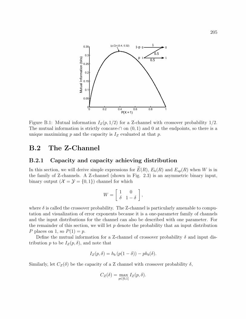
205

0 0.2 0.4 0.6 0.8 10

0.05

0.1

0.15

0.2

0.25

0.3

0.35

Mu

tual

In

form

atio

n (b

its)

P(X = 1)

(p,C)= (0.4, 0.32)

1 1

0 01

p

1-p

0.5

0.5

Figure B.1: Mutual information IZ(p, 1/2) for a Z-channel with crossover probability 1/2.The mutual information is strictly concave-∩ on (0, 1) and 0 at the endpoints, so there is aunique maximizing p and the capacity is IZ evaluated at that p.

B.2 The Z-Channel

B.2.1 Capacity and capacity achieving distribution

In this section, we will derive simple expressions for E(R), Eh(R) and Esp(R) when W is inthe family of Z-channels. A Z-channel (shown in Fig. 2.3) is an asymmetric binary input,binary output (X = Y = 0, 1) channel for which

W =

[1 0δ 1− δ

],

where δ is called the crossover probability. The Z-channel is particularly amenable to compu-tation and visualization of error exponents because it is a one-parameter family of channelsand the input distributions for the channel can also be described with one parameter. Forthe remainder of this section, we will let p denote the probability that an input distributionP places on 1, so P (1) = p.

Define the mutual information for a Z-channel of crossover probability δ and input dis-tribution p to be IZ(p, δ), and note that

IZ(p, δ) = hb (p(1− δ))− phb(δ).

Similarly, let CZ(δ) be the capacity of a Z channel with crossover probability δ,

CZ(δ) = maxp∈[0,1]

IZ(p, δ).

206

Since IZ(p, δ) is strictly concave-∩ (see Fig. B.1) for δ ∈ [0, 1), it follows that there is aunique capacity achieving p for each δ.

Proposition 16. Let p∗(δ) denote the capacity achieving p for a Z-channel with crossoverprobability δ. Then, for all δ ∈ [0, 1),

p∗(δ) =

[(1− δ)

(1 + exp

(hb(δ)

1− δ

))]−1, (B.8)

and

CZ(δ) = hb (p∗(δ)(1− δ))− p∗(δ)hb(δ)

= hb

([1 + exp

(hb(δ)

1− δ

)]−1)− hb(δ)

(1− δ)(

1 + exp(hb(δ)1−δ

)) . (B.9)

A plot of p∗(δ) is shown in Fig. 2.5 and a plot of CZ(δ) is given in Fig. 2.4.

Proof: Assume that all log’s and exponentials are base e. Then, for t ∈ (0, 1),

dhb(t)

dt= log

1− tt

,

and hence,

∂IZ(p, δ)

∂δ=

∂

∂p[hb (p(1− δ))− phb(δ)]

= (1− δ) log1− p(1− δ)p(1− δ)

− hb(δ).

Now, IZ(p, δ) is strictly concave-∩ in p, nonnegative and IZ(0, δ) = IZ(1, δ) = 0, so we canset the derivative to 0 and solve for p to yield the capacity achieving p∗(δ) in (B.8). ThenCZ(δ) = IZ(p∗(δ), δ), yielding (B.9).

B.2.2 Evaluating error exponents

The mutual information IZ(p, δ) is convex-∪ in δ for a fixed p and the capacity, CZ(δ) isconvex-∪ in δ as it is the maximum of a set of convex-∪ functions. It is easy to see as wellthat both are strictly decreasing in δ. The range of CZ(δ) is [0, 1], so let it’s inverse functionbe, for R ∈ [0, 1],

f(R) , C−1Z (R) = minβ ∈ [0, 1] : CZ(β) ≤ R. (B.10)

207

0 0.2 0.4 0.6 0.8 10

0.05

0.1

0.15

0.2

0.25

0.3

0.35

0.4

0.45

0.5

1 1

0 01

0.1

0.9

1-

I (0

.1, )

Z

h (0.1)b

Figure B.2: IZ(p, δ) is a strictly decreasing, convex-∪ function of δ for all p ∈ (0, 1). It isplotted here for p = 0.1. The left endpoint is hb(p).

Similarly, for a fixed p ∈ [0, 1], the range of IZ(p, δ) is [0, hb(p)] (see Fig. B.2), so forR ∈ [0, hb(p)], let the inverse function be denoted

g(R, p) , I−1Z (p,R) = minβ ∈ [0, 1] : IZ(p, β) ≤ R. (B.11)

Both f(R) and g(R, p) are well defined, convex-∪ and strictly monotonically decreasing withR (for all p ∈ (0, 1) for g(R, p)).

We will evaluate the three exponents Eh(R), E(R) and Esp(R) when W is a Z-channelwith crossover probability δ. For all three exponents, it will be sufficient to consider testchannels V that are also Z-channels. The reason is that if a binary input, binary outputchannel V has V (0|1) > 0, then D(V ||W |P ) = ∞ if P (1) > 0. Therefore, no such channelwould be included in the minimizations over channels V for the exponents. Now, if V is aZ-channel with crossover probability β, then

D(V ||W |P ) =∑

x,y∈0,1

P (x)V (y|x) logV (y|x)

W (y|x)

= P (0)× 0 + P (1)

[β log

β

δ+ (1− β) log

1− β1− δ

]= P (1)Db(β||δ),

where Db(β||δ) denotes the binary divergence

Db(β||δ) , β logβ

δ+ (1− β) log

1− β1− δ

.

208

Proposition 17. If W is a Z-channel with crossover probability δ, then, for R ∈ [0, CZ(δ)],

Eh(R) = Db (f(R)||δ)E(R) = pr(R, δ)Db (f(R)||δ)

Esp(R) = maxp∈[0,1]:IZ(p,δ)≥R

pDb (g(R, p)||δ) ,

where g and f are defined in (B.11) and (B.10) respectively and

pr(R, δ) , maxp ∈ [0, 1] : IZ(p, δ) ≥ R.

Proof: First,

Eh(R) = minβ∈[0,1]:CZ(β)≤R

maxp∈[0,1]

pDb(β||δ).

The inner maximization is independent of β, and Db is nonnegative so p = 1 is the maximizer.Also, since CZ(β) is monotonically decreasing and R ≤ CZ(δ), and Db(β||δ) is increasing inβ for β ≥ δ, it follows that the minimizing β is f(R).

Second,

E(R) = minβ∈[0,1]:CZ(β)≤R

maxp∈[0,1]:IZ(p,δ)≥R

pDb(β||δ).

Similarly to the argument for Eh(R), the maximizing p in the inner max is the largest p suchthat I(p, δ) ≥ R, which we denote pr(R, δ), and the minimizing β is f(R).

Finally,

Esp(R) = maxp∈[0,1]

minβ:IZ(p,β)≤R

pDb(β||δ)

= maxp∈[0,1]:IZ(p,δ)≥R

minβ:IZ(p,β)≤R

pDb(β||δ)

= maxp∈[0,1]:IZ(p,δ)≥R

Esp(R, p)

Esp(R, p) , minβ:IZ(p,β)≤R

pDb(β||δ)

= pDb (g(R, p)||δ) ,

where we may as well remove p such that I(p, δ) < R because Esp(R, p) evaluates to 0for those p (as Db(δ||δ) = 0). Similarly to CZ(β), for a fixed p, IZ(p, β) is monotonicallydecreasing in β. For those p that have IZ(p, δ) ≥ R, the set of β that have IZ(p, β) < R alllie to the right of δ, hence the minimizing β is g(R, p).

Obtaining an analytical expression for the maximizing p in Esp(R) seems to be difficult.Fig. B.3 shows a plot of Esp(R, p), and it can be seen to be non-concave-∩, but quasi-concave(∩) in p. Define the sphere-packing optimizing p to be

p∗sp(R, δ) , arg maxp∈[0,1]:IZ(p,δ)≥R

Esp(R, p).

209

0.1 0.2 0.3 0.4 0.5 0.6 0.7 0.80

0.005

0.01

0.015

0.02

0.025

0.03

0.035

p = P(X = 1)

(p,E) = (.47, .035)

E (

0.2,

p)sp

1 1

0 01

p

1-p

0.5

0.5R =0.2 bits/use

Figure B.3: A plot of Esp(R, p) in base 2 for R = 0.2 (bits/channel use), when δ = 0.5,CZ(δ) = 0.322 bits/channel use. As a function of p, Esp(R, p) is not concave-∩, but isquasi-concave.

Figure 2.6 shows a plot of p∗sp(R, δ) for δ = 0.5 and R near capacity. As can be seen fromthe figure, p∗sp(R, δ) approaches p∗(δ) from above as R→ CZ(δ) with a non-zero slope.

The expressions in Proposition 17 can be used to quickly plot the three exponents, asshown in Fig. 3.1, because evaluating the inverse functions of CZ and IZ can be done inlogarithmic time as the accuracy desired tends to 0. Evaluating the max over p for Esp isdone by brute force.

B.2.3 Exponents near capacity

Proposition 18. If W is a Z-channel of crossover probability δ ∈ (0, 1),

limR→CZ(δ)

Eh(R)

Esp(R)≥ 1

p∗(δ)≥ 2.

Proof: We know that Eh(R) = Db(f(R)||δ). Now, since CZ(f(R)) = R, this means thatfor all p ∈ [0, 1], IZ(p, f(R)) ≤ R, hence we can upper bound Esp(R) as

Esp(R) ≤ maxp∈[0,1]:IZ(p,δ)≥R

pDb(f(R)||δ)

= pr(R, δ)Db(f(R)||δ).

210

Using the fact that limR→CZ(δ) pr(R, δ) = p∗(δ) yields

limR→CZ(δ)

Eh(R)

Esp(R)≥ lim

R→CZ(δ)

Db(f(R)||δ)pr(R, δ)Db(f(R)||δ)

=1

limR→CZ(δ) pr(R, δ)

=1

p∗(δ).

For all values of δ ∈ [0, 1), p∗(δ) ≤ 1/2.

With regards to E(R), it can be seen from a plot (Fig. 3.3) that

limR→CZ(δ)

E(R)

Esp(R)= 1.

This fact can also be proved by looking at Taylor expansions of the two exponents aroundcapacity.

Proposition 19. If W is a Z-channel with crossover probability δ ∈ (0, 1),

limR→CZ(δ)

E(R)

Esp(R)= 1.

Proof: First, fix a δ and let C = CZ(δ). It is straightforward to check that the second-order expansion of Db(δ + ε||δ) around ε = 0 is

Db(δ + ε||δ) =ε2

2δ(1− δ)+O(ε3),

where the notation O(ε3) means that there are constants K > 0 and εK > 0 such that if|ε| ≤ εK ,

|O(ε3)| ≤ K|ε|3.

Now, recall that

E(R) = pr(R, δ)Db(f(R)||δ).

where pr(R, δ) is the largest p such that IZ(p, δ) ≥ R and f(R) is the inverse function ofCZ(β) defined in (B.10). By continuity2 of IZ(p, δ) there is a real valued function k(·) suchthat

pr(R, δ) = p∗(δ) + k(R− C),

2IZ(p, δ) has a derivative of 0 at p = p∗(δ), hence the first derivative of pr(R, δ) at C is undefined, i.e.−∞. That does not prevent us from using continuity however.

211

and limt→0 k(t) = 0. Note also that f(R) has a Taylor expansion about R = C, which is

f(R) = δ + f ′(C)(R− C) +O(|R− C|2).

Using these expansions, we have

E(R) = (p∗(δ) + k(R− C))×Db

(δ + f ′(C)(R− C) +O(|R− C|2)||δ

)= (p∗(δ) + k(R− C))×

[(f ′(C)(R− C) +O(|R− C|2))2

2δ(1− δ)+O(|R− C|3)

]

= (p∗(δ) + k(R− C))×[f ′(C)2(R− C)2

2δ(1− δ)+O(|R− C|3)

]=p∗(δ)f ′(C)2

2δ(1− δ)(R− C)2 +

f ′(C)2

2δ(1− δ)(R− C)2k(R− C) +O(|R− C|3). (B.12)

Now, we already know that Esp(R) ≤ E(R) for all R, so we want a lower bound on Esp(R),because a simple expression for the sphere-packing optimizing p∗sp(R, δ) is lacking. Hence,we take the lower bound

Esp(R) = maxp:IZ(p,δ)≥R

pDb(g(R, p)||δ)

≥ p∗(δ)Db(g(R, p∗(δ))||δ).

Having fixed p = p∗(δ) for all R, we can define the function of one variable,

g(R) , g(R, p∗(δ)).

We can take a Taylor expansion of g to yield

g(R) = δ + g′(C)(R− C) +O((R− C)2).

Plugging this into the lower bound for Esp(R) gives

Esp(R) ≥ p∗(δ)Db

(δ + g′(C)(R− C) +O((R− C)2)||δ

)= p∗(δ)

[(g′(C)(R− C) +O(|R− C|2))2

2δ(1− δ)+O(|R− C|3)

]

= p∗(δ)

[g′(C)2(R− C)2

2δ(1− δ)+O(|R− C|3)

]=p∗(δ)g′(C)2

2δ(1− δ)(R− C)2 +O(|R− C|3). (B.13)

212

At this point, we would like to show that f ′(C) = g′(C). Since f(R) is the inverse functionof CZ(β), it follows that

f ′(C) =

[dCZ(β)

dβ

∣∣∣∣β=δ

]−1.

Now, CZ(β) = IZ(p∗(β), β), so by chain rule,

C ′Z(β) = ∇IZ(p, τ)

∣∣∣∣(p,τ)=(p∗(β),β)

·

[dp∗(τ)

dτ

∣∣∣∣τ=β

1

]

=

[∂Iz(p, β)

∂p

∣∣∣∣p=p∗(β)

∂IZ(p∗(β), τ)

∂τ

∣∣∣∣τ=β

]·

[dp∗(τ)

dτ

∣∣∣∣τ=β

1

],

where · denotes dot product in the above. Since p∗(β) is the capacity achieving p for β, itfollows by concavity of IZ(p, β) in p that

∂Iz(p, β)

∂p

∣∣∣∣p=p∗(β)

= 0

C ′Z(δ) =∂IZ(p∗(δ), τ)

∂τ

∣∣∣∣τ=δ

.

Now, g(R) = g(R, p∗(δ)) is the inverse function of IZ(p∗(δ), β) when viewed as a function ofβ. Therefore,

g′(R) =

[∂IZ(p∗(δ), β)

∂β

∣∣∣∣β:IZ(p∗(δ),β)=R

]−1

g′(C) =

[∂IZ(p∗(δ), β)

∂β

∣∣∣∣β=δ

]−1

=

[dCz(β)

dβ

∣∣∣∣β=δ

]−1= f ′(C).

Therefore, using the fact that f ′(C) = g′(C) and the expansions of (B.12) and (B.13),

1 ≤ limR→C

E(R)

Esp(R)≤ lim

R→C

p∗(δ)f ′(C)2

2δ(1−δ) (R− C)2 + f ′(C)2

2δ(1−δ)(R− C)2k(R− C) +O(|R− C|3)p∗(δ)g′(C)2

2δ(1−δ) (R− C)2 +O(|R− C|3)

= limR→C

1 + k(R− C)/p∗(δ) +O(|R− C|)1 +O(|R− C|)

= 1,

where the last line follows because k(R− C)→ 0 as R→ C.

213

0

1

0

e

1 1 1

0 0

1-1-

1- 0

11

1

1 |||

1

Figure B.4: Simulating a Z-channel by using a BEC and collapsing the erasure symbol into0.

B.2.4 The back-story bound for the Z-channel

Let Efb(R;Z(δ)) denote the error exponent with feedback for the Z-channel with crossoverprobability δ. and let Esp(R;BEC(δ)) denote the sphere-packing exponent for the BECwith erasure probability δ. It is readily seen that for R ∈ [0, 1− δ],

Esp(R;BEC(δ)) = Db(1−R||δ)

and we have already seen that

Efb(R;Z(δ)) ≤ Eh(R;Z(δ)) = Db(C−1Z (R)||δ).

Now, one can simulate Z(δ) with BEC(δ) as shown in Figure B.4 by collapsing the erasuresymbol and 0 into 0 at the output of the BEC. We know from the ‘back-story’ bound that

Efb(R;Z(δ)) ≤ Esp(R;BEC(δ)).

The question then becomes whether Esp(R;BEC(δ)) < Eh(R;Z(δ) or not. From the plot ofCZ(δ) in Figure 2.4, we know that CZ(β) ≤ 1− β for all β ∈ [0, 1] (with strict inequality forβ ∈ (0, 1)). Therefore, 1−R > C−1Z (R) > δ if δ ∈ (0, 1). Therefore

Esp(R;BEC(δ)) = Db(1−R||δ)> Db(C

−1Z (R)||δ)

= Eh(R;Z(δ)).

So the back-story bound is not tighter than Haroutunian if we use a BEC as the back-storyfor a Z-channel. It seems unlikely to get a different result by using a larger channel than theBEC as the back-story to the Z-channel. Numerical evaluations of the BSC followed by aZ-channel as the back-story to a binary asymmetric channel have also not yielded anythingtighter than the Haroutunian bound.

214

Appendix C

Arbitrarily varying sources appendix

C.1 The cheating switcher with clean observations

Theorem 9 of Section 4.3: Define the set of distributions

C =

∑

x∈V p(x) ≥ P(∀ l, xl ∈ V

)p : ∀ V such that

V ⊆ X

,

where the event ∀ l, xl ∈ V is shorthand for (x1, . . . , xm) : xl ∈ V , l = 1, . . . ,m. Also,define

R(D) , maxp∈C

R(p,D).

For a general set of distributions Q ⊂ P(X ), let Dmin(Q) , supp∈QDmin(p). Suppose theswitcher has either 1-step lookahead or full lookahead. In both cases, for D > Dmin(C),

R(D) = R(D)

For D < Dmin(C), R(D) = ∞ by convention because the switcher can simulate a distri-bution for which the distortion D is infeasible for the coder.

C.1.1 Achievability for the coder

The main tool of the proof is:

Lemma 26 (Type Covering). Let SD(xn) , xn ∈ X n : dn(xn, xn) ≤ D be the set of

X n strings that are within distortion D of a given X n string xn. Fix an ε > 0. Then forall n ≥ n0(d, ε), for any p ∈ Pn(X ), there exists a codebook B = xn(1), xn(2), . . . , xn(M)where M ≤ exp(n(R(p,D) + ε)) and

T np ⊆⋃

xn∈B

SD(xn),

215

where T np is the set of X n strings with type p.

Proof: See [47], Lemma 2.4.1. Note that n0(d, ε) is independent of both p and D.

We now show how the coder can get arbitrarily close to R(D) for large enough n. For aδ > 0,

Cδ ,

∑

x∈V p(x) ≥ P (∀l, xl ∈ V)− δp ∈ P : ∀ V such that

V ⊆ X

.

Lemma 27 (Converse for switcher). Let ε > 0. For all n sufficiently large

1

nlnM(n,D) ≤ R(D) + ε.

Proof: Fix a λ > 0 and λ ≤ λ(ε) < D−Dmin(C) to be defined later. We know R(p,D−λ) is a continuous function of p ( [47]). It follows then that because Cδ is monotonicallydecreasing (as a set) with δ that for all ε > 0, there is a δ > 0 so that

maxp∈Cδ

R(p,D − λ) ≤ maxp∈C

R(p,D − λ) + ε/3.

We will have the coder use a codebook such that all X n strings with types in Cδ are coveredwithin distortion D−λ. The coder can do this for large n with at most M codewords in thecodebook B, where

M ≤ (n+ 1)|X | exp

(n

(maxp∈Cδ

R(p,D − λ) + ε/3

))≤ exp(n(max

p∈CR(p,D − λ) + ε)).

Explicitly, this is done by taking a union of the codebooks provided by the type-coveringlemma and noting that the number of types in Pn(X ) is less than (n + 1)|X |. Next, we willshow that the probability of the switcher being able to produce a string with a type not inCδ goes to 0 exponentially with n.

Consider a type p ∈ Pn(X )∩ (P(X )−Cδ). By definition, there is some V ⊆ X such that∑x∈V p(x) < P (xl ∈ V , 1 ≤ l ≤ m)− δ. Let ζk(V) be the indicator function

ζk(V) =m∏l=1

1(xl,k ∈ V).

ζk indicates the event that the switcher cannot output a symbol outside of V at time k. Thenζk(V) is a Bernoulli random variable with a probability of being 1 equal to κ(V) , P (xl ∈V , 1 ≤ l ≤ m). Since the subsources are IID over time, ζk(V) is a sequence of IID binaryrandom variables with distribution q′ , (1− κ(V), κ(V)).

216

Now for the type p ∈ Pn(X )∩(P(X )−Cδ), we have that for all strings xn in the type classTp,

1n

∑ni=1 1(xi ∈ V) < κ(V)− δ. Let p′ be the binary distribution (1− κ(V) + δ, κ(V)− δ).

Therefore ||p′− q′||1 = 2δ, and hence we can bound the binary divergence D(p′||q′) ≥ 2δ2 byPinsker’s inequality. Using standard types properties [21] gives

P

(1

n

n∑k=1

ζk(V) < κ(V)− δ)≤ (n+ 1) exp(−nD(p′||q′))

≤ (n+ 1) exp(−2nδ2).

This bound holds for all V ⊂ X ,V 6= ∅, so we sum over types not in Cδ to get

P (pxn /∈ Cδ) ≤∑

p∈Pn(X )∩(P(X )−Cδ)

(n+ 1) exp(−2nδ2)

≤ (n+ 1)|X | exp(−2nδ2)

= exp

(−n(

2δ2 − |X | ln(n+ 1)

n

)).

Then, regardless of the switcher strategy,

E[d(xn;B)] ≤ D − λ+ d∗ × exp

(− n

(2δ2 − |X | ln(n+ 1)

n

)).

So for large n we can get arbitrarily close to distortion D − λ while the rate is at mostmaxp∈C R(p,D−λ) + ε. Using the fact that the IID rate-distortion function is continuous inD (uniformly over p such that Dmin(p) < D, see (C.8)) gives us that the coder can achieve

at most distortion D on average while the asymptotic rate is at most R(D) + 2ε (provided

λ ≤ λ(ε) is small enough). Since ε is arbitrary, R(D) ≤ R(D).

C.1.2 Achievability for the switcher

This section shows that R(D) ≥ R(D) when the switcher has 1-step lookahead. We willshow that the switcher can target any distribution p ∈ C and produce a sequence of IIDsymbols with distribution p. In particular, the switcher can target the distribution thatyields maxp∈C R(p,D), so R(D) ≥ R(D).

The switcher will use a memoryless randomized strategy. Let V ⊆ X and suppose thatat some time k the set of symbols available to choose from for the switcher is exactly V , i.e.x1,k, . . . , xm,k = V . Recall β(V) , P (x1,1, . . . , xm,1 = V) is the probability that at anytime the switcher must choose among elements of V and no other symbols. Then let f(x|V)be a probability distribution on X with support V , i.e. f(x|V) ≥ 0, ∀ x ∈ X , f(x|V) = 0if x /∈ V , and

∑x∈V f(x|V) = 1. The switcher will have such a randomized rule for every

217

nonempty subset V of X such that |V| ≤ m. Let D be the set of distributions on X thatcan be achieved with these kinds of rules,

D =

p(·) =

∑V⊆X ,|V|≤m β(V)f(·|V),

p : ∀ V s.t. V ⊆ X , |V| ≤ m,f(·|V) is a PMF on V

.

It is clear by construction that D ⊆ C because the conditions in C are those that onlyprevent the switcher from producing symbols that do not occur enough on average, but putno further restrictions on the switcher. So we need only show that C ⊆ D. The followinggives such a proof by contradiction.

Lemma 28 (Achievability for switcher). The set relation C ⊆ D is true.

Proof: Without loss of generality, let X = 1, . . . , |X |. Suppose p ∈ C but p /∈ D. It isclear that D is a convex set. Let us view the probability simplex in R|X |. Since D is a convexset, there is a hyperplane through p that does not intersect D. Hence, there is a vector(a1, . . . , a|X |) such that

∑|X |i=1 aip(i) = t for some real t but t < minq∈D

∑|X |i=1 aiq(i). Without

loss of generality, assume a1 ≥ a2 ≥ . . . ≥ a|X | (otherwise permute symbols). Now, we will

construct f(·|V) so that the resulting q has∑|X |

i=1 aip(i) ≥∑|X |

i=1 aiq(i), which contradicts theinitial assumption. Let

f(i|V) ,

1 if i = max(V)0 else

,

so for example, if V = 1, 5, 6, 9, then f(9|V) = 1 and f(i|V) = 0 if i 6= 9. Call q thedistribution on X induced by this choice of f(·|V). Recall that κ(V) = P (xl ∈ V , 1 ≤ l ≤ m).Then, we have

|X |∑i=1

aiq(i) = a1κ(1) + a2[κ(1, 2)− κ(1)] +

· · ·+ a|X |

[κ(1, . . . , |X |)− κ(1, . . . , |X | − 1)

]By the constraints in the definition (4.3) of C, we have the following inequalities for p:

p(1) ≥ κ(1) = q(1)

p(1) + p(2) ≥ κ(1, 2) = q(1) + q(2)...

|X |−1∑i=1

p(i) ≥ κ(1, . . . , |X | − 1) =

|X |−1∑i=1

q(i).

218

Therefore, the difference of the objective is

|X |∑i=1

ai(p(i)− q(i)) = a|X |

[ |X |∑i=1

p(i)− q(i)]

+

(a|X |−1 − a|X |)[ |X |−1∑

i=1

p(i)− q(i)]

+

· · ·+ (a1 − a2)[p(1)− q(1)

]=

|X |−1∑i=1

(ai − ai+1)

[ i∑j=1

p(j)−i∑

j=1

q(j)

]≥ 0.

The last step is true because of the monotonicity in the ai and the inequalities we derivedearlier. Therefore, we see that

∑|X |i=1 aip(i) ≥

∑|X |i=1 aiq(i) for the p we had chosen at the be-

ginning of the proof. This contradicts the assumption that∑|X |

i=1 aip(i) < minq∈D∑|X |

i=1 aiq(i),therefore it must be that C ⊆ D.

C.2 Adversarial switching with noisy observations

Theorem 10 of Section 4.4: For the AVS problem of Fig. 4.2, where the adversary hasaccess to the states either with 1-step lookahead or full lookahead,

R(D) = maxp∈Dstates

R(p,D),

where

Dstates =

p :

p(·) =∑

t∈T α(t)f(·|t)f(·|t) ∈ G(t),∀ t ∈ T

.

Proof: It is clear that R(D) ≥ maxp∈Dstates R(p,D) because the switcher can selectdistributions f(·|t) ∈ G(t) for all t ∈ T and upon observing a state t, the switcher canrandomly select the switch position according to the convex combination that yields f(·|t).With this strategy, the AVS is simply an IID source with distribution p(·) =

∑t α(t)f(·|t).

Hence, R(D) ≥ maxp∈Dstates R(p,D).We will now show that R(D) ≤ maxp∈Dstates R(p,D). This can be done in the same way

as in Appendix C.1. We can use the type covering lemma to cover sequences with types inor very near Dstates and then we need only show that the probability of xn having a typeε-far from Dstates goes to 0 with block length n.

219

Lemma 29. Let pxn be the type of xn and for ε > 0 let Dstates,ε be the set of p ∈ P(X ) withL1 distance at most ε from a distribution in Dstates. Then, for ε > 0,

P (pxn /∈ Dstates,ε) ≤ 4|T ||X | exp(−nξ(ε)),

where ξ(ε) > 0 for all ε > 0. So for large n, pxn is in Dstates,ε with high probability.

Proof: Let tn be the n-length vector of the observed states. We assume that the switcherhas advance knowledge of all these states before choosing the switch positions. First, we showthat with high probability, the states that are observed are strongly typical. Let N(t|tn) bethe count of occurrence of t ∈ T in the vector tn. Fix a δ > 0 and for t ∈ T , define the event

Atδ =

∣∣∣∣N(t|tn)

n− α(t)

∣∣∣∣ > δ

. (C.1)

Since N(t|tn) =∑n

i=1 1(ti = t) and each term in the sum is an IID Bernoulli variable withprobability of 1 equal to α(t), we have by Hoeffding’s tail inequality [57],

P (Atδ) ≤ 2 exp(−2nδ2).

Next, we need to show that the substrings output by the AVS at the times when thestate is t have a type in or very near G(t). This will be done by a martingale argumentsimilar to that given in Lemma 3 of [4]. Let t∞ denote the infinite state sequence (t1, t2, . . .)and let F0 = σ(t∞) be the sigma field generated by the states t∞. For i = 1, 2, . . ., letFi = σ(t∞, si,xi1, . . . ,x

im). Note that Fi∞i=0 is a filtration and for each i, xi is included in

Fi trivially because xi = xsi,i.Let Ci be the |X |-dimensional unit vector with a 1 in the position of xi. That is, Ci(x) =

1(xi = x) for each x ∈ X . Define Ti to be

Ti = Ci − E[Ci|Fi−1]

and let S0 = 0. For k ≥ 1,

Sk =k∑i=1

Ti.

We claim that Sk, k ≥ 1 is a martingale1 with respect to the filtration Fi defined previously.To see this, note that E[|Sk|] <∞ for all k since Sk is bounded (not uniformly). Also, Sk ∈ Fkbecause Ti ∈ Fi for each i. Finally,

E[Sk+1|Fk] = E[Tk+1 + Sk|Fk]= E[Tk+1|Fk] + Sk

= E[Ck+1 − E[Ck+1|Fk]|Fk] + Sk

= E[Ck+1|Fk]− E[Ck+1|Fk] + Sk

= Sk.

1Sk is a vector, so we show that each component of the vector is a martingale. For ease of notation, wedrop the dependence on the component of the vector until it is explicitly needed.

220

Now, define for each t ∈ T ,T ti = Ti · 1(ti = t)

and analogously,

Stk =k∑i=1

T ti .

It can be easily verified that Stk is a martingale with respect to Fi for each t ∈ T .Expanding, we also see that

1

N(t|tn)Stn =

1

N(t|tn)

n∑i=1

Ti1(ti = t)

=1

N(t|tn)

∑i: ti=t

Ci −

1

N(t|tn)

∑i: ti=t

E[Ci|Fi−1]. (C.2)

The first term in the difference above is the type of the output of the AVS during timeswhen the state is t. For any i such that ti = t,

E[Ci|Fi−1] =m∑l=1

P (l|Fi−1)pl(·|t) ∈ G(t).

In the above, P (l|Fi−1) represents the switcher’s possibly random strategy because theswitcher chooses the switch position at time i with knowledge of events in Fi−1. The symbolgenerator’s outputs, conditioned on the state at the time are independent of all other ran-dom variables, so

∑ml=1 P (l|Fi−1)pl(·|t) is the probability distribution of the output at time

i conditioned on Fi−1.Thus, the second term in the difference of (C.2) is in G(t) because it is the average of

N(t|tn) terms in G(t) and G(t) is a convex set. Therefore, Stn/N(t|tn) measures the differencebetween the type of symbols output at times when the state is t and some distributionguaranteed to be in G(t).

Let pxn be the empirical type of the string xn, and let ptxn be the empirical type of thesub-string of xn corresponding to the times i when ti = t. Then,

pxn =∑t∈T

N(t|tn)

nptxn .

Let G(t)ε be the set of distributions at most ε in L1 distance from a distribution in G(t).Recall that for |X | dimensional vectors, ‖p− q‖∞ < ε/|X | implies ‖p− q‖1 < ε. Hence, we

221

have

P

(⋃t∈T

ptxn /∈ G(t)ε

)≤

∑t∈T

P

(⋃x∈X

∣∣∣∣ 1

N(t|tn)Stn(x)

∣∣∣∣ > ε

|X |

)

≤∑t

∑x

P

(∣∣∣∣ 1

N(t|tn)Stn(x)

∣∣∣∣ > ε

|X |

). (C.3)

Let (Atδ)c denote the complement of the event Atδ. So, for every (t, x) we have

P

(∣∣∣∣ 1

N(t|tn)Stn(x)

∣∣∣∣ > ε

|X |

)≤ P (Atδ) + P

(∣∣∣∣ 1

N(t|tn)Stn(x)

∣∣∣∣ > ε

|X |, (Atδ)

c

)≤ 2 exp(−2nδ2) +

P

(∣∣∣∣ 1

N(t|tn)Stn(x)

∣∣∣∣ > ε

|X |, (Atδ)

c

).

In the event of (Atδ)c, we have N(t|tn) ≥ n(α(t)− δ), so

P

(∣∣∣∣ 1

N(t|tn)Stn(x)

∣∣∣∣ > ε

|X |, (Atδ)

c

)≤ P

(|Stn(x)| > n(α(t)− δ) ε

|X |, (Atδ)

c

)≤ P

(|Stn(x)| > n(α(t)− δ) ε

|X |

).

Stk(x) is a martingale with bounded differences since |Stk+1(x) − Stk(x)| = |T tk+1(x)| ≤ 1.Hence, we can apply Azuma’s inequality [58] to get

P

(∣∣∣∣ 1

N(t|tn)Stn(x)

∣∣∣∣ > ε

|X |, (Atδ)

c

)≤ 2 exp

(−n(α(t)− δ)2ε2

2|X |2

). (C.4)

Plugging this back into (C.3),

P

(⋃t∈T

ptxn /∈ G(t)ε

)≤ 2|T ||X |

(exp(−2nδ2) +

exp

(−n(α∗ − δ)2ε2

2|X |2

))≤ 4|X ||T | exp(−nξ(ε, δ))

where

ξ(ε, δ) = min

2δ2,

(α∗ − δ)2ε2

2|X |2

α∗ , min

t∈Tα(t).

222

We assume without loss of generality that α∗ > 0 since T is finite. We will soon need thatδ ≤ ε/|T |, so let

ξ(ε) = max0<δ<minε/|T |,α∗

ξ(ε, δ)

and note that it is always positive provided ε > 0, since ξ(ε, δ) > 0 whenever δ ∈ (0, α∗).Hence,

P

(⋃t∈T

ptxn /∈ G(t)ε

)≤ 4|X ||T | exp(−nξ(ε)).

We have shown that with probability at least 1 − 4|X ||T | exp(−nξ(ε)), for each t ∈ Tthere is some pt ∈ G(t) such that ‖ptxn − pt‖1 ≤ ε and (Atε/|T |)

c occurs. Let

p =∑t∈T

α(t)pt.

By construction, p ∈ Dstates. To finish, we show that ‖pxn − p‖1 ≤ 2ε.

‖pxn − p‖1 =∑x∈X

|pxn(x)− p(x)|

=∑x

∣∣∣∣∣∑t∈T

N(t|tn)

nptxn(x)− α(t)pt(x)

∣∣∣∣∣≤

∑t

∑x

∣∣∣∣N(t|tn)

nptxn(x)− α(t)pt(x)

∣∣∣∣=

∑t

α(t)∑x

∣∣∣∣N(t|tn)

nα(t)ptxn(x)− pt(x)

∣∣∣∣≤

∑t

α(t)∑x

|ptxn(x)− pt(x)|+∣∣∣∣N(t|tn)

nα(t)− 1

∣∣∣∣ ptxn(x).

From (C.1), we are assumed to be in the event that∣∣∣∣N(t|tn)

nα(t)− 1

∣∣∣∣ ≤ δ

α(t)

Hence,

‖pxn − p‖1 ≤∑t

α(t)

(ε+

δ

α(t)

)= ε+ |T |δ ≤ 2ε.

We have proved P (pxn /∈ Dstates,2ε) ≤ 4|X ||T | exp(−nξ(ε)), so we arrive at the conclusion of

the lemma by letting ξ(ε) = ξ(ε/2).

223

C.3 Uniform continuity of R(p,D)

Lemma 9 of Section 4.7.1:Let d : X×X → [0, d∗] be a distortion function. d is the minimum nonzero distortion from

(4.1). Also, assume that for each x ∈ X , there is an x0(x) ∈ X such that d(x, x0(x)) = 0.

Then, for p, q ∈ P(X ) with ‖p− q‖1 ≤ d4d∗

, for any D ≥ 0,

|R(p,D)−R(q,D)| ≤ 7d∗

d‖p− q‖1 ln

|X ||X |‖p− q‖1

.

Proof: Let W ∗p,D ∈ argminW∈W(p,D)I(p,W ). Then

|R(p,D)−R(q,D)| = |I(p,W ∗p,D)− I(q,W ∗

q,D)|.

Consider d(p,W ∗q,D), the distortion of source p across q’s distortion D achieving channel.

d(p,W ∗q,D) ≤ d(q,W ∗

q,D) + |d(p,W ∗q,D)− d(q,W ∗

q,D)|≤ D + ‖p− q‖1d∗.

By definition, W ∗q,D is in W(p, d(p,W ∗

q,D)), so R(p, d(p,W ∗q,D)) ≤ I(p,W ∗

q,D).

R(p, d(p,W ∗q,D)) ≤ I(p,W ∗

q,D)

≤ |I(p,W ∗q,D)− I(q,W ∗

q,D)|+ I(q,W ∗q,D)

= |I(p,W ∗q,D)− I(q,W ∗

q,D)|+R(q,D) (C.5)

Expanding mutual informations yields

|I(p,W ∗q,D)− I(q,W ∗

q,D)| ≤ |H(p)−H(q)|+ |H(pW ∗q,D)−H(qW ∗

q,D)|+|H(p,W ∗

q,D)−H(q,W ∗q,D)|.

Above, for a distribution p on X and channel W from X to X , H(pW ) denotes the entropy

of a distribution on X with probabilities (pW )(x) =∑

x p(x)W (x|x). H(p,W ) denotes the

entropy of the joint source on X × X with probabilities (p,W )(x, x) = p(x)W (x|x). It isstraightforward to verify that ‖pW − qW‖1 ≤ ‖p− q‖1 and ‖(p,W )− (q,W )‖1 ≤ ‖p− q‖1.So using Lemma 8 three times, we have

|I(p,W ∗q,D)− I(q,W ∗

q,D)| = |I(p,W ∗q,D)− I(q,W ∗

q,D)|

≤ 3‖p− q‖1 ln|X ||X |‖p− q‖1

.

224

Now, we have seen d(p,W ∗q,D) ≤ D + d∗‖p − q‖1. We will use the uniform continuity of

R(p,D) in D to bound |R(p,D)−R(p,D + d∗‖p− q‖1)|. This will give an upper bound onR(p,D)−R(q,D) as seen through (C.5), namely,

R(p,D)−R(q,D) ≤ |I(p,W ∗q,D)− I(q,W ∗

q,D)|+R(p,D)−R(p, d(p,W ∗

q,D))

≤ |I(p,W ∗q,D)− I(q,W ∗

q,D)|+R(p,D)−R(p,D + d∗‖p− q‖1), (C.6)

where the last step follows because R(p,D) is monotonically decreasing in D. For a fixed p,the rate-distortion function in D is convex-∪ and decreasing and so has steepest descent atD = 0. Therefore, for any 0 ≤ D1, D2 ≤ d∗,

|R(p,D1)−R(p,D2)| ≤ |R(p, 0)−R(p, |D2 −D1|)|.

Hence, we can restrict our attention to continuity of R(p,D) around D = 0. By assumption,W(p, 0) 6= ∅ ∀p ∈ P(X ). Now consider an arbitrary D > 0, and let W ∈ W(p,D). We willshow that there is some W0 ∈ W(p, 0) that is close to W in an L1-like sense (relative to thedistribution p). Since W ∈ W(p,D), we have by definition

D ≥∑x

p(x)∑x

W (x|x)d(x, x)

=∑x

p(x)∑

x: d(x,x)>0

W (x|x)d(x, x)

≥ d∑x

p(x)∑

x: d(x,x)>0

W (x|x). (C.7)

Now, we will construct a channel in W(p, 0), denoted W0. First, for each x, x such thatd(x, x) = 0, let V (x|x) = W (x|x). For all other (x, x), set V (x|x) = 0. Note that V is nota channel matrix if W /∈ W(p, 0) since it is missing some probability mass. To create W0,for each x, we redistribute the missing mass from V (·|x) to the pairs (x, x) with d(x, x) = 0.Namely, for (x, x) with d(x, x) = 0, we define

W0(x|x) = V (x|x) +

∑x′: d(x,x′)>0W (x′|x)

|x′ : d(x, x′) = 0|.

For all (x, x) with d(x, x) > 0, define W0(x|x) = 0. So, W0 is a valid channel in W(p, 0).

225

Now for a fixed x ∈ X ,∑x

|W (x|x)−W0(x|x)| =∑

x: d(x,x)>0

W (x|x) +∑

x: d(x,x)=0

|W (x|x)−W0(x|x)|

=∑

x: d(x,x)>0

W (x|x) +∑

x: d(x,x)=0

∣∣∣∣∣∑

x′: d(x,x′)>0W (x′|x)

|x′ : d(x, x′) = 0|

∣∣∣∣∣= 2

∑x: d(x,x)>0

W (x|x).

Therefore, using (C.7) ∑x

p(x)∑x

|W (x|x)−W0(x|x)| ≤ 2D

d.

So, for W = W ∗p,D, there is a W0 ∈ W(p, 0) with the above ‘modified L1 distance’ with respect

to p betweenW andW0 being less than 2D/d. Going back to the bound on |R(p, 0)−R(p,D)|,

|R(p, 0)−R(p,D)| = minW∈W(p,0)

I(p,W )− I(p,W ∗p,D)

≤ I(p,W0)− I(p,W ∗p,D)

≤ |H(pW0)−H(pW ∗p,D)|+ |H(p,W0)−H(p,W ∗

p,D)|.

It can be easily verified that ‖pW0 − pW ∗p,D‖1 is at most 2D/d. Similarly, ‖(p,W0) −

(p,W ∗p,D)‖1 ≤ 2D/d.

Now, assuming D ≤ d/4, we can again invoke Lemma 8 to get

|R(p, 0)−R(p,D)| ≤ 2D

dlnd|X |2D

+2D

dlnd|X ||X |

2D

≤ 4D

dlnd|X ||X |

2D. (C.8)

Going back to (C.6), we see that if ‖p− q‖1 ≤ d4d∗

,

|R(p,D + d∗‖p− q‖1)−R(p,D)| ≤ 4d∗‖p− q‖1d

lnd|X ||X |

2d∗‖p− q‖1

≤ 4d∗‖p− q‖1d

ln|X ||X |‖p− q‖1

.

226

The last step follows because d/d∗ ≤ 1. Substituting into (C.6) gives

R(p,D)−R(q,D) ≤ 3‖p− q‖1 ln|X ||X |‖p− q‖1

+ 4d∗

d‖p− q‖1 ln

|X ||X |‖p− q‖1

≤ 7d∗

d‖p− q‖1 ln

|X ||X |‖p− q‖1

.

Finally, this bound holds uniformly on p and q as long as the condition on ‖p−q‖1 is satisfied.Therefore, we can interchange p and q to get the other side of the inequality

R(q,D)−R(p,D) ≤ 7d∗

d‖p− q‖1 ln

|X ||X |‖p− q‖1

.

C.4 Proof of Lemma 10

We now assume d : X × X → [0, d∗] to be arbitrary. However, we let

d0(x, x) = d(x, x)−minx∈X

d(x, x)

so that Lemma 9 applies to d0. Let R0(p,D) be the IID rate-distortion function for p ∈ P(X )at distortion D with respect to distortion measure d0(x, x). By definition, R(p,D) is the IIDrate-distortion function for p with respect to distortion measure d(x, x). From Problem 13.4of [21], for any D ≥ Dmin(p),

R(p,D) = R0(p,D −Dmin(p)).

Hence, for p, q ∈ P(X ), D ≥ max(Dmin(p), Dmin(q)),

|R(p,D)−R(q,D)| = |R0(p,D −Dmin(p))−R0(q,D −Dmin(q)|≤ |R0(p,D −Dmin(p))−R0(p,D −Dmin(q))|+|R0(p,D −Dmin(q))−R0(q,D −Dmin(q))|. (C.9)

Now, we note that |Dmin(p)−Dmin(q)| ≤ d∗‖p− q‖1. The first term of (C.9) can be boundedusing (C.8) and the second term of (C.9) can be bounded using Lemma 9. The first term

can be bounded if ‖p− q‖1 ≤ d0/4d∗ and the second can be bounded if ‖p− q‖1 ≤ d0/4d

∗0.

Since d∗0 ≤ d∗, we only require ‖p− q‖1 ≤ d0/4d∗.

|R(p,D)−R(q,D)| ≤ 4d∗

d0‖p− q‖1 ln

d0|X ||X |2d∗‖p− q‖1

+

7d∗0

d0‖p− q‖1 ln

|X ||X |‖p− q‖1

≤ 11d∗

d0‖p− q‖1 ln

|X ||X |‖p− q‖1

.

227

Bibliography

[1] C. E. Shannon, “A mathematical theory of communication,” The Bell System TechnicalJournal, vol. 27, pp. 379–423, 623–656, 1948.

[2] ——, “The zero-error capacity of a noisy channel,” IRE Trans. Inform. Theory, vol. 2,pp. 8–19, 1956.

[3] E. Haroutunian, “Lower bound for error probability in channels with feedback,” Prob-lemy Peredachi Informatsii, pp. 36–44, 1977.

[4] T. Berger, “The source coding game,” IEEE Trans. Inf. Theory, vol. 17, pp. 71–76, Jan.1971.

[5] C. Shannon, “Channels with side information at the transmitter,” IBM J. Res. Devel.,vol. 2, pp. 289–293, Oct. 1958.

[6] S. Gelfand and M. Pinsker, “Coding for channel with random parameters,” Probl. Pered.Inform. (Probl. Inf. Transm.), vol. 9, pp. 19–31, 1980.

[7] C. Heegard and A. Gamal, “On the capacity of computer memory with defects,” Infor-mation Theory, IEEE Transactions on, vol. 29, no. 5, pp. 731 – 739, sep 1983.

[8] S. Jafar, “Capacity with causal and noncausal side information: A unified view,” Infor-mation Theory, IEEE Transactions on, vol. 52, no. 12, pp. 5468 –5474, dec. 2006.

[9] M. V. Burnashev, “Data transmission over a discrete channel with feedback,” ProblemyPeredachi Informatsii, vol. 12, p. 1030, 1976.

[10] B. Nakiboglu, “Exponential bounds on error probability with feedback,” Ph.D. disser-tation, Massachussetts Institute of Technology, Cambridge, MA, 2011.

[11] Y. Polyanskiy, “Channel coding: non-asymptotic fundamental limits,” Ph.D. disserta-tion, Princeton University, Princeton, NJ, 2010.

[12] A. Feinstein, “A new basic theorem of information theory,” IRE Trans. Inform. Theory,vol. 4, pp. 2–22, 1954.

228

[13] ——, “Error bounds in noisy channels without memory,” IRE Trans. Inform. Theory,vol. 1, pp. 13–14, 1955.

[14] P. Elias, “Coding for nosiy channels,” in IRE Natl. Conv. Rec., 1955, pp. 37–46.

[15] R. M. Fano, Transmission of Information. Cambridge, MA and New York, NY: MITPress and Wiley, 1961.

[16] R. G. Gallager, “A simple derivation of the coding theorem and some applications,”vol. 11, pp. 3–18, Jan. 1965.

[17] R. Gallager, Information Theory and Reliable Communication. New York, NY: JohnWiley and Sons, 1971.

[18] C. Shannon, R. Gallager, and E. Berlekamp, “Lower bounds to error probability forcoding on discrete memoryless channels. I,” Information and Control, vol. 10, pp. 65–103, 1967.

[19] E. A. Haroutunian, “Estimates of exponents in error probability for a semicontinuousmemoryless channel,” Problemy Peredachi Informatsii, pp. 37–48, 1968.

[20] R. Blahut, “Hypothesis testing and information theory,” Information Theory, IEEETransactions on, vol. 20, no. 4, pp. 405 – 417, Jul. 1974.

[21] T. Cover and J. Thomas, Elements of Information Theory. New York, NY: John Wileyand Sons, 1991.

[22] C. Shannon, R. Gallager, and E. Berlekamp, “Lower bounds to error probability forcoding on discrete memoryless channels. II,” Information and Control, vol. 10, pp. 522–552, 1967.

[23] K. S. Zigangirov, “Upper bounds for the error probability for channels with feedback,”Problems of Information Transmission, vol. 6, pp. 87–92, 1970.

[24] A. G. D’yachkov, “Upper bounds on the error probability for discrete memoryless chan-nels with feedback,” Problems of Information Transmission, vol. 11, pp. 13–28, 1975.

[25] M. V. Burnashev, “On the reliability function of a binary symmetrical channel withfeedback,” Problems of Information Transmission, vol. 24, pp. 3–10, 1988.

[26] R. Dobrushin, “Asymptotic estimate of error probability in message transmissionthrough memoryless channels using feedback,” Problemy Kibernetiki [Russian], pp. 161–168, 1962.

229

[27] E. Haroutunian, “Estimation of optimal error probability in information transmissionthrough channels with feedback,” in Proceedings of the Fourth All-Union Symposiumon Redundancy in Infomation Systems [In Russian], Leningrad, USSR, 1970.

[28] ——, “Lower bound of error probability in data transmission through channels withfeedback,” in Proceedings of the Second International Symposium on Information Theory[In Russian], Tsakhkadzor, Armenia, 1971, pp. 12–13.

[29] Y. Polyanskiy, H. V. Poor, and S. Verdu, “Channel coding rate in the finite blocklengthregime,” IEEE Trans. Inf. Theory, vol. 56, pp. 2307–2359, May 2010.

[30] A. Y. Sheverdyaev, “Lower bound for error probability in a discrete memoryless channelwith feedback,” Problemy Peredachi Informatsii, pp. 5–15, 1982.

[31] H. Palaiyanur and A. Sahai, “An upper bound for the block coding error exponent withdelayed feedback,” in Proc. Int. Symp. Inform. Theory, Austin, TX, Jun. 2010.

[32] I. Csiszar, “The method of types [information theory],” Information Theory, IEEETransactions on, vol. 44, no. 6, pp. 2505 –2523, Oct. 1998.

[33] B. Nakiboglu, Personal Communication, 2008-2009.

[34] U. Augustin, “Noisy channels,” Habilitationschrift at Universitat-Nurenberg. Submittedto Springer Lecture Notes, 1978.

[35] T. S. Han, Information-Spectrum Methods in Information Theory, 1st ed. Heidelberg,Germany: Springer-Verlag, 2002.

[36] G. Como and B. Nakiboglu, “A lower bound on the error probability for block-codeswith finite memory feedback,” in Proc. Int. Symp. Inform. Theory, Austin, TX, Jun.2010.

[37] A. Sahai, “Why do block length and delay behave differently if feedback is present,”IEEE Trans. Inf. Theory, vol. 54, pp. 1860–1886, May 2008.

[38] A. Sahai and P. Grover, “The price of certainty: waterslide curves and the gap tocapacity,” 2008. [Online]. Available: http://arxiv.org/abs/0801.0352

[39] A. Sahai and S. Draper, “The hallucination bound for the bsc,” in Proc. Int. Symp.Inform. Theory, Toronto, Canada, Jul. 2008.

[40] A. Sahai and S. Mitter, “The necessity and sufficiency of anytime capacity for stabi-lization of a linear system over a noisy communication link - part I: Scalar systems,”vol. 52, no. 8, pp. 3369–3395, Aug. 2006.

230

[41] R. Bajcsy, “Active perception,” Proceedings of the IEEE, vol. 76, no. 8, pp. 966–1005,Aug. 1988.

[42] T. Berger and J. Gibson, “Lossy source coding,” IEEE Trans. Inf. Theory, vol. 44, no. 6,pp. 2693–2723, Oct 1998.

[43] J. Ziv, “Distortion-rate theory for individual sequences,” IEEE Trans. Inf. Theory,vol. 26, no. 2, pp. 137–143, Mar 1980.

[44] E.-H. Yang and J. Kieffer, “Simple universal lossy data compression schemes derivedfrom the lempel-ziv algorithm,” IEEE Trans. Inf. Theory, vol. 42, pp. 239–245, 1996.

[45] R. Ahlswede, “Extremal properties of rate-distortion functions,” IEEE Trans. Inf. The-ory, vol. 36, pp. 166–171, Jan. 1990.

[46] H. Palaiyanur, C. Chang, and A. Sahai, “The source coding game with a cheatingswitcher,” To appear in IEEE Transactions on Information Theory, 2011.

[47] I. Csiszar and J. Korner, Information Theory: Coding Theorems for Discrete Memory-less Systems, 2nd ed. New York, NY: Academic Press, 1997.

[48] C. Shannon, “Coding theorems for a discrete source with a fidelity criterion,” in IRENatl. Conv. Rec., 1959, pp. 142–163.

[49] J. Wolfowitz, “Approximation with a fidelity criterion,” in 5th Berkeley Symp. on Math.Stat. and Prob., vol. 1. Berkeley, California: University of California, Press, 1967, pp.565–573.

[50] D. Sakrison, “The rate-distortion function for a class of sources,” Information andControl, vol. 15, pp. 165–195, Mar. 1969.

[51] M. Harrison and I. Kontoyiannis, “Estimation of the rate-distortion function,” 2007.[Online]. Available: http://arxiv.org/abs/cs/0702018v1

[52] T. Weissman, E. Ordentlich, G. Seroussi, S. Verdu, and M. L. Weinberger, “Inequalitiesfor the l1 deviation of the empirical distribution,” Hewlett-Packard Labs, Tech.Rep., 2003. [Online]. Available: http://www.hpl.hp.com/techreports/2003/HPL-2003-97R1.html

[53] D. Neuhoff and R. K. Gilbert, “Causal source codes,” IEEE Trans. Inf. Theory, vol. 28,pp. 701–713, Sep. 1982.

[54] R. Dobrushin, “Unified methods for the transmission of information: The general case,”Sov. Math., vol. 4, pp. 284–292, 1963.

231

[55] A. Lapidoth and P. Narayan, “Reliable communication under channel uncertainty,”IEEE Trans. Inf. Theory, vol. 44, Oct. 1998.

[56] G. Hardy, J. Littlewood, and G. Polya, Inequalities, 2nd ed. Cambridge, UK: Cam-bridge University Press, 1952.

[57] W. Hoeffding, “Probability inequalities for sums of bounded random variables,” Journalof the American Statistical Association, vol. 58, no. 301, pp. 13–30, Mar 1963.

[58] K. Azuma, “Weighted sums of certain dependent random variables,” Tohoku Math.Journal, vol. 19, pp. 357 – 367, 1967.