the fews index: fixed effects with a window · pdf filethe fews index: fixed effects with a...

The FEWS index: Fixed effects with a window splice Non-revisable quality-adjusted price indexes with no characteristic information

Paper presented at the meeting of the group of experts on consumer price indices, at Geneva, Switzerland

26–28 May 2014

Frances Krsinich1

Senior Researcher, Prices Unit, Statistics New Zealand P O Box 2922

Wellington, New Zealand [email protected]

1 The author would like to thank Richard Arnold, Alberto Cavallo, Alistair Gray, Jan de Haan, Pilar Iglesias, Chris Pike, and Soon Song for their support and contributions to this work.

Crown copyright © This work is licensed under the Creative Commons Attribution 3.0 New Zealand licence. You are free to copy, distribute, and adapt the work, as long as you attribute the work to Statistics NZ and abide by the other licence terms. Please note you may not use any departmental or governmental emblem, logo, or coat of arms in any way that infringes any provision of the Flags, Emblems, and Names Protection Act 1981. Use the wording 'Statistics New Zealand' in your attribution, not the Statistics NZ logo.

Liability The opinions, findings, recommendations, and conclusions expressed in this paper are those of the author. They do not represent those of Statistics New Zealand, which takes no responsibility for any omissions or errors in the information in this paper.

Citation Krsinich F (2014, May). The FEWS index: Fixed effects with a window splice. Paper presented at the meeting of the group of experts on consumer price indices, Geneva, Switzerland.

http://creativecommons.org/licenses/by/3.0/nz/deed.en

http://www.legislation.govt.nz/act/public/1981/0047/latest/DLM51358.html

http://www.legislation.govt.nz/act/public/1981/0047/latest/DLM51358.html

http://creativecommons.org/licenses/by/3.0/nz/deed.en

Abstract This paper describes the approach Statistics New Zealand is considering to estimate quality-adjusted price indexes from scanner and online data where there is no information on product characteristics. Matched-model methods can be biased, as they don’t reflect the implicit price changes associated with products being introduced and disappearing. This potential bias is likely to become more significant over time with increasing technological change. We show that the relatively simple fixed-effects (or time-product dummy) index is equivalent to a fully interacted time-dummy hedonic index based on all price-determining characteristics of the products, despite those characteristics not being observed. In production, this can be combined with a modified approach to splicing that incorporates the price movement across the full estimation window to reflect new products with one period’s lag, without requiring revision. Empirical results for this fixed-effects window-splice (FEWS) index are presented for different data sources: three years of New Zealand consumer electronics scanner data from market research company GfK; six years of United States supermarket scanner data from market research company IRI; and 15 months of New Zealand consumer electronics daily online data from MIT's Billion Prices Project.

1. IntroductionEnsuring that consumer price indexes reflect only price change is important, and is traditionally achieved by pricing a fixed basket of goods over time. However, products such as consumer electronics are rapidly evolving, and have correspondingly shorter life cycles in the market. This makes the traditional approach of pricing a representative fixed basket challenging. The potential for using ‘big data’ such as scanner and online data to measure price change with higher accuracy and frequency makes this issue of rapid product change even more challenging. Price measurement needs to use the data available and be easily automatable. Carefully crafted hedonic models that select different sets of characteristics for each product are not a feasible approach in a production environment. Comprehensive information on product characteristics generally isn’t available, and the time and expertise needed to develop and maintain these kinds of models are prohibitive. Price measurement based on scanner data has been an active area of research for Statistics NZ over the last five years. Collaborative research with Statistics Netherlands (de Haan and Krsinich, 2014a) on a new method called the imputation Tornqvist RYGEKS (ITRYGEKS) has established it as benchmark index which appropriately quality-adjusts, both for the changing quality-mix of products being bought, and for the implicit price movements of new products entering, and old products disappearing, from the market. Based on this research, Statistics NZ intends to incorporate consumer electronics scanner data into production for the New Zealand consumers price index in the September quarter of 2014, using the ITRYGEKS method. Supermarket scanner data and online data, however, do not contain sufficient information on characteristics for us to be able to use the ITRYGEKS method. This has led us to revisit the fixed-effects index (also known as the ‘time-product dummy’ (TPD) index) that we used in benchmarking the New Zealand housing rentals index (Krsinich, 2011). Because the fixed-effects index requires at least two price observations before a new product is non-trivially incorporated into the estimation, we have incorporated a modified approach to the splicing2 – the ‘window splice’. This uses the movement across the entire estimation window,

2 Because consumer price indexes tend to be non-revisable, we can’t update the estimated index, so a standard approach is to ‘splice’ on the most recently estimated movement to the previously published index number.

3

The FEWS index: Fixed effects with a window splice, by Frances Krsinich

rather than just the movement of the most recent period. This effectively revises for the implicit price movements associated with the introduction of new products, in the period after their introduction. We call this combined approach the fixed-effects window-splice (FEWS) index3. The FEWS approach allows us to produce non-revisable and fully quality-adjusted price indexes where there is longitudinal price and quantity information at a detailed product specification level. In this paper, we will show theoretically and empirically that the fixed-effects index is equivalent to a fully interacted time-dummy hedonic index based on all characteristics that are constant across time at the barcode level. We also show empirically that this fully-interacted time-dummy hedonic index is virtually the same as the more common main-effects time-dummy hedonic index when a full set of price-determining characteristics is included in the hedonic model. The paper is structured as follows: Section 2 gives the background to the development of the FEWS index by Statistics NZ – from benchmarking the housing rentals index, to evaluating this approach in the context of both supermarket scanner data and online data, and then incorporating fixed-effects indexes for mobile phones and televisions in the New Zealand import price index from the December 2013 quarter. Section 3 aims to motivate an intuitive understanding of how the fixed-effects index can appropriately quality-adjust, despite having no explicit information on characteristics, by using a simplified visual demonstration of the way the longitudinal price record of a new product is fit around the underlying price movement of matched products. In section 4, we restate a result from de Haan and Hendriks (2013) for the main-effects time-dummy4 hedonic index in terms of categorical characteristics. We then extend it to include interactions between characteristics as well as main effects, to show that the fixed-effects index is algebraically equivalent to a fully-interacted time-dummy hedonic index that explicitly incorporates all characteristics of the products5. In section 5, we use a simulation to demonstrate that a fully-interacted time-dummy hedonic index and the fixed-effects index give the same results when the product identifiers used in the fixed-effects index are based on the same set of characteristics included in the time-dummy hedonic index. Section 6 describes how the window splice incorporates implicit revisions in the most recent estimation window’s movement to optimise the quality of the long-term index, in particular by revising for the implicit price movements of new products entering the market in the period after their introduction.

3 Until recently, we have been referring to the fixed-effects index as a ‘time-product dummy’ (TPD) index, with its non-revisable production counterpart called the ‘rolling year time-product dummy’ (RYTPD). In Krsinich (2013), we referred to the RYTPD combined with the window splice as the ‘RYTPD with a modified splice’ and used the acronym RY’TPD to denote it. This terminology has become unwieldy, so we have now adopted ‘fixed-effects window-splice’ (FEWS) as a more descriptive and simpler name, with a pronounceable acronym. 4 That is, the hedonic model that explicitly incorporates characteristics of products. 5 Actually, on all characteristics that are constant across time at the level of the product-identifier. For scanner data or online data, this is all characteristics, as any change in the characteristic of a product is accompanied by a changed barcode or model name.

4


We present empirical results for the FEWS index in section 7 for a range of data sources, with gradually less information available in each case:

• New Zealand monthly-aggregated consumer electronics scanner data from marketresearch company GfK, with characteristics and quantities

• United States weekly-aggregated supermarket scanner data from IRI, with quantitiesbut no characteristics

• New Zealand daily consumer electronics web-scraped online data from the BillionPrices Project, with no characteristics or quantities.

In section 8, we rank all the feasible methods that might be used in the case of scanner or online data, on a range of criteria. Section 9 concludes.

2. BackgroundHedonic regression has been used in producing the New Zealand consumers price index for over 10 years, to measure quality-adjusted price movements of used cars using a time-dummy hedonic index based on a rolling eight-quarter estimation window. To put this into production, the most recently estimated quarter’s6 movement is spliced onto the previous index number each quarter7. The hedonic approach was then used to retrospectively benchmark the performance of the current matched-sample approach to measuring the price movement of housing rentals. However, due to the lack of sufficient characteristics in the housing rental survey data, we exploited the longitudinal nature of the data by fitting a fixed-effects model to implicitly control for all time-invariant characteristics of the rental dwellings. ‘Fixed effects’ is a term used in a variety of ways, depending on the field. We follow Allison (2005) in using it to refer to fitting product-specific (or dwelling-specific, in the case of the housing rentals index) intercepts into the regression model. Allison explains fixed-effects methods as follows:

(p2) … by using [fixed-effects] it is possible to control for all possible characteristics of the individuals [or product] in the study – even without measuring them – so long as those characteristics do not change over time. (p3) The essence of a fixed-effects method is captured by saying that each individual [or product] serves as his or her [or its] own control. That is accomplished by making comparison within individuals (hence the need for at least two measurements), and then averaging those differences across all the individuals in the sample.

This approach was controversial at the time, and so in Krsinich (2011) we extended a result from Aizcorbe, Corrado, and Doms (2003) to show that the implicit price movement being estimated for new rental dwellings by the retrospective fixed-effects index was appropriate8. In de Haan and Krsinich (2014a), which presents and empirically tests the imputation Tornqvist rolling year GEKS (ITRYGEKS) index, it was noted that the fixed-effects index, referred to as the rolling year time-product dummy (RYTPD) index, tended to sit closer to the benchmark ITRYGEKS than did the RYGEKS, which similarly uses only product identifiers rather than explicitly incorporating information on characteristics. This was noted then as an unexpected result requiring further research.

6 The New Zealand consumers price index is currently a quarterly index. 7 This approach is monitored every quarter by overlaying the successive eight-quarter indexes over one another to check for ‘drift’. To date, they are very stable across time, which gives us confidence that splicing on the most recent quarter is a valid approach for used cars. 8 Note that, for reasons discussed in section 3, the fixed-effects index requires at least two observations for a dwelling (or product) before it is non-trivially included in the estimation. This means that the retrospective fixed-effects index used to benchmark the rental index reflected new dwellings for all but the last quarter of the period examined.

5


Krsinich (2013) then modified the fixed-effects index by splicing on the movement across the entire window rather than just the movement of the most recent period. This was a simplified version of a suggestion by Melser (2011) for improving the splicing of the RYGEKS. This further improved the performance of the fixed-effect index, against the benchmark ITRYGEKS. In Krsinich (2013), it was first noted that the time-product dummy index appears to be equivalent to a fully interacted time-dummy hedonic model and, therefore, might do an even better job of quality-adjusting than the ITRYGEKS (which incorporates main-effects time-dummy hedonic bilateral indexes). Initially, we had assumed that the fixed-effects index was only partially quality-adjusting, based on its tendency to sit between the RYGEKS and the ITRYGEKS indexes. De Haan and Hendriks (2013) explored using the fixed-effects index for producing high-frequency price indexes from online data, deriving expressions for both the time-dummy hedonic and fixed-effects indexes. These, we show in this paper, are equivalent when the time-dummy hedonic index is restated in terms of categorical characteristics and extended to incorporate all the interactions between characteristics. However, seemingly biased empirical results for women’s t-shirts9, along with their belief that ‘measuring quality-adjusted price indexes without information on item characteristics is just not possible’, led the authors to conclude that the fixed-effects index is not appropriate for products where quality change is important. In the December 2013 quarter, Statistics NZ introduced fixed-effects indexes into production for the New Zealand import price index, for mobile phones and televisions. For the major brands of these two products, we have comprehensive data on import prices and quantities at a detailed product level. Because the previous quarter of the New Zealand import price index is revisable, we have not needed to incorporate the window splicing – instead, we revise the previous quarter’s movement to incorporate the new products’ price movements. We are likely to consider using FEWS indexes for supermarket products in the New Zealand consumers price index if we can get full-coverage scanner data from the major supermarket chains. After some initial research on New Zealand consumer electronics daily online data, shared with us by the Billion Prices Project at MIT and presented in section 7.3, we have entered into a research agreement with PriceStats10, who will be collecting and processing daily online data for us to investigate, for a wide range of major New Zealand retailers with strong online presences.

3. IntuitionWe will try here to motivate an intuitive understanding of how the fixed-effects method works with a simplified example. First, consider four products, all with the same set of characteristics. The characteristics are fixed across time. The standard approach to hedonic modelling fits the log of price against characteristics and time, so we can visualise the graphs of logged price for each product as follows. Pred P1 is the predicted logged price for the base product P1, and actual logged prices for each of the four products P1 to P4 differs from this predicted P1 each period by a normally distributed error term.

9 Our hypothesis (which could be easily tested) about the bias in the women’s t-shirts index in de Haan and Hendriks (2013) is that, because fashion is highly seasonal, there was probably an almost-complete replacement of old products with new products between seasons. The only matched products on which to base the fixed effects estimation (see section 3 for the intuition behind this) would be products undergoing heavy discounting. This suggests that a condition for using the fixed-effects index might be that there is at least some minimum percentage of products that are matched, and not undergoing seasonal discounting, between any two successive periods. 10 See www.pricestats.com

6

http://www.pricestats.com/


Figure 1 All products with the same characteristics

Now consider the situation where the products each have different characteristics from one another, and these characteristics are fixed across time at the product level – as they would be in the case of scanner data or online data, where barcodes or product names change if there is a change in characteristics. We assume that, within the estimation window of the hedonic model, characteristics’ parameters are constant. Another, perhaps more useful, way of stating this is that we are estimating the average parameter for each characteristic over the estimation window. The net effect of each product’s characteristics is constant over time, so the logged price is moved up or down by this constant factor accordingly. This constant factor is the ‘fixed effect’ estimated by the fixed-effects model – the product-specific intercept.

Figure 2 Each product with a different set of characteristics

7


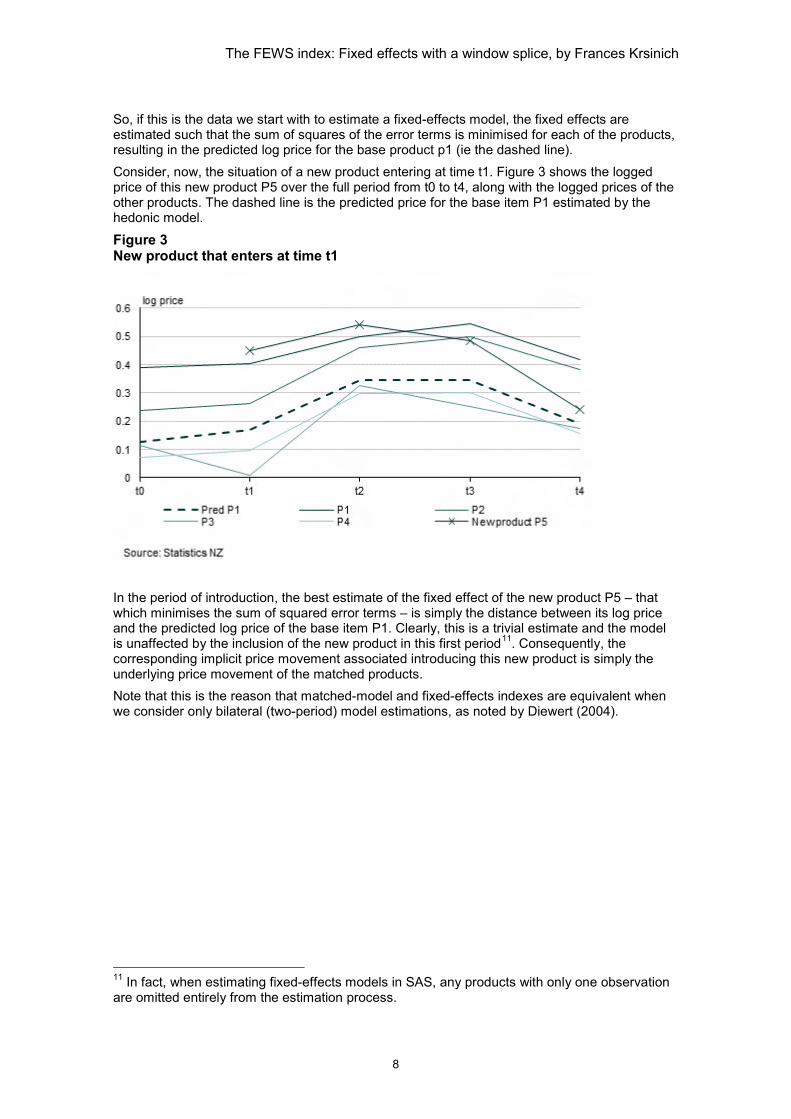
So, if this is the data we start with to estimate a fixed-effects model, the fixed effects are estimated such that the sum of squares of the error terms is minimised for each of the products, resulting in the predicted log price for the base product p1 (ie the dashed line). Consider, now, the situation of a new product entering at time t1. Figure 3 shows the logged price of this new product P5 over the full period from t0 to t4, along with the logged prices of the other products. The dashed line is the predicted price for the base item P1 estimated by the hedonic model.

Figure 3 New product that enters at time t1

In the period of introduction, the best estimate of the fixed effect of the new product P5 – that which minimises the sum of squared error terms – is simply the distance between its log price and the predicted log price of the base item P1. Clearly, this is a trivial estimate and the model is unaffected by the inclusion of the new product in this first period11. Consequently, the corresponding implicit price movement associated introducing this new product is simply the underlying price movement of the matched products. Note that this is the reason that matched-model and fixed-effects indexes are equivalent when we consider only bilateral (two-period) model estimations, as noted by Diewert (2004).

11 In fact, when estimating fixed-effects models in SAS, any products with only one observation are omitted entirely from the estimation process.

8


Figure 4 Period of introduction of new product P5

The second price observation of P5 enables a more meaningful estimate of the fixed effect of new product P5 (and consequently of the implicit price movement associated with its introduction), as shown in figure 5. This can be visualised as moving the price movement of P5 up or down until the sum of squares of the error terms (indicated with bold lines) is minimised. Note that to keep things simple for the purpose of this example, we’re assuming the underlying predicted price movement of the base product P1 is unaffected by the new product P5. Of course in practice, the predicted price will be slightly affected by the new product and it is the appropriate estimation of this new product’s fixed effect (and therefore its influence on the resulting price index) that we’re ultimately interested in.

9


Figure 5 Second price observation period for new product P5

As more prices are observed for the new product p5, the estimate of its fixed effect is updated accordingly. Figures 6 and 7 show how the estimate of the fixed effect gradually reduces each period as a result of fitting the longitudinal logged price record for this new product around the underlying logged price movement of the other products.

Figure 6 Third price observation period for new product P5

10


Figure 7 Fourth price observation period for new product P5

Because the estimate of the fixed effect is trivial in the first period, at least two price observations are required before a new product can contribute meaningfully to the estimation. And with more price observations, the estimate of the fixed effect for the new product converges to its true value – that is, the estimate is being driven more by the shape of the longitudinal price record than by the error terms. So, in production, if just the most recent period’s movement is spliced on, as with methods such as the rolling year GEKS (RYGEKS) or the rolling year time-dummy (RYTD) hedonic indexes, then the contribution of new products to the index will be systematically missed and the index will be correspondingly biased. To get around this problem in production, we propose a different approach to the splicing, where the movement across the entire estimation window (usually one year plus a period –ie five quarters or 13 months) is incorporated. This form of revision enables the implicit price movements associated with new products to be incorporated, and allows the estimate of the fixed effect to be gradually updated with more price observations. This window splicing is discussed further in section 6.

4. Theory In this section, we extend results from de Haan and Hendriks (2013) to show that, when all characteristics are treated as categorical, the fully interacted time-dummy hedonic index is the same as the fixed-effects index where the characteristics included in the time-dummy hedonic models are those that correspond to product identifiers. In the case of scanner data, where barcodes change with any change in a price-determining characteristic, this means the fixed-effects index (with barcodes as the product identifiers) is equivalent to a fully interacted time-dummy hedonic index where all price-determining characteristics are explicitly included in the hedonic model.

11


4.1 The main-effects time-dummy hedonic index As discussed in de Haan and Hendriks (2013), the unweighted12 time-dummy hedonic index13 can be expressed as follows.

−== ∑

∏

∏=

∈

∈K

k

tkkk

Si

Ni

Si

Nti

ttTD zz

p

pP

t

t

ME1

01

0

1

0 )(êxp)(

)()êxp(

0

0

βδ ; (t= 1,…,T) (1)

Where tip is the price of item (ie product) i in time t, tN is the number of items in time t, k

iz is

the quantity of characteristic k for item i and kβ̂ is the estimate of the corresponding parameter.

Note that the item i is the tightly defined product – that is, the product as defined by the barcode (for scanner data) or model name (for online data). The exponential factor is the quality-adjustment factor, which adjusts the ratio of geometric mean prices for any changes in the average characteristics of products between period t and the base period 0.

We can, and do, treat all characteristics as categorical. This is realistic, as we’re considering the characteristics corresponding to a discrete set of product specifications. That is, even numeric characteristics such as ‘screen size’ for computers or ‘number of pixels’ for cameras will take a discrete set of values across the set of product specifications. Note that any change in a characteristic in scanner data corresponds to a change in barcode (or, in online data, a change in characteristic corresponds to a changed product identifier, or model name), and therefore the number of characteristics is discrete (as a consequence of the number of barcodes or product identifiers being discrete). Note also that the treatment of characteristics as categorical is an advantage if there are missing or unknown values of any of the characteristics, as these can be given the category value ‘missing’ or ‘unknown’ and therefore kept in the estimation, which keeps the data as representative as possible, and uses all the rest of the information in the data. By treating the characteristics as categorical, we are not imposing any parametric form on the hedonic model. Because we are conditioning based on the characteristics, rather than building predictive models, and because we tend to have so much data available in scanner and online data, this is a valid modelling approach. With all the characteristics being modelled as categorical, we can restate (1) as follows.

−== ∑

∏

∏=

∈

∈L

l

tlll

Si

Ni

Si

Nti

ttTD DD

p

pP

t

t

ME1

0

10

1

0 )(êxp)(

)()êxp(

0

0

βδ

; (t= 1,…,T) (2) Where L is the total number of categories across the k characteristics, less k (ie we omit a base category for each of the k characteristics) and t

lD is the proportion of tSi∈ with the

characteristic lD .

12 They also extend the formulation to the weighted case. For simplicity, we restrict this theory section to the unweighted case, but our simulation in section 5 shows that the equivalence of the two indexes also holds in the weighted case. 13 Including main-effects only, which we make explicit here by using the ME subscript

12


4.2 The fully-interacted time-dummy hedonic index We can follow the same reasoning as in de Haan and Hendriks (2013) to get an equivalent expression to (2) for the fully-interacted time-dummy hedonic index. That is, the index derived from a hedonic model that includes the main effects and all the interactions14 between characteristics. For simplicity, and without loss of generality, we will consider products with just two characteristics15. The estimating equation for the full hedonic model can be written as follows.

(3)

Where tip is the price of item i in period t; ilD are the dummy variables for the L main effects

and imD are the dummy variables for the M second-order interactions, with lβ and mβ the

corresponding parameters; 0δ is the intercept; tδ are the time-dummy parameters (from which the index is derived); and t

iε are the random errors.

Appendix 1 follows the approach of de Haan and Hendriks (2013) to give the full derivation from (3), of the fully-interacted time-dummy hedonic index shown in equation (4).

−+−== ∑ ∑

∏

∏= =

∈

∈L

l

M

m

tmmm

tlll

Si

Ni

Si

Nti

ttTD DDDD

p

pP

t

t

full1 1

001

0

1

0 )(ˆ)(êxp)(

)()êxp(

0

0

ββδ

; (t=1,…,T) (4) This is the time-dummy hedonic index with quality adjustment for the change in characteristics in terms of not only the main effects, but all the interactions of characteristics. So the quality adjustment is more comprehensive than that of the main-effects time-dummy index of equation (2).

4.3 The fixed-effects index De Haan and Hendriks (2013) show that the fixed-effects index can be formulated as follows.

[ ]t

Si

Ni

Si

Nti

ttFE

p

pP t

t

γγδ ˆêxp)(

)()êxp( 0

10

1

0

0

0

−==

∏

∏

∈

∈

(5)

14 For n characteristics this would be the main-effects, the two-way interactions, the three-way interactions, and so on up to the n-way interactions. 15 For example, characteristics A and B, each of which has three categories 1, 2, and 3. The four main effects correspond to the dummy variables for each of A1, A2, A3, B1, B2, and B3 (less the two base categories for each of characteristics A and B). The eight second-order interactions are the dummy variables for each of A1B1, A1B2,…, A3B3 (less one base category).

ti

M

mimmil

L

ll

T

t

ti

tti DDDp εββδδ ++++= ∑∑∑

=== 111

0ln

13


Where ∑∈= 0

00 /ˆˆSi i Nγγ

and ∑∈= tSi

ti

t N/ˆˆ γγ are the sample means of the estimated

fixed effects. The exponential terms in (4) and (5) are the same, because the fixed effect for any item i is, by definition, the net effect of the parameters corresponding to the ‘bundle’ of characteristics belonging to i, where the characteristics are constant across time at the item, or product, level. That is, the fixed effect is the sum of the parameters on the main effects and all the interactions for the characteristics of the item, or product. To illustrate, we can use the example given in footnote 15, and consider an item with the characteristics A3 and B1 in time t. In the fully-interacted time-dummy hedonic index formulation of equation (4), this item will

contribute 1313ˆˆˆ

BABA βββ ++ to the expression in the brackets which, when exponentiated, is the quality-adjustment factor.

In the fixed-effects index formulation of equation (5), the item contributes a fixed effect of iγ̂ to the corresponding bracketed term. Since, by definition, the fixed effect is the net effect of the

characteristics of the item, 1313ˆˆˆˆ BABAi βββγ ++= .

So, the fixed-effects index and the fully-interacted time-dummy hedonic index are exactly the same. The following section demonstrates this empirically for the weighted case (using expenditure shares as weights) by using a subset of three characteristics to both include in the fully-interacted time-dummy hedonic index and to define the product identifiers used in the fixed-effects index.

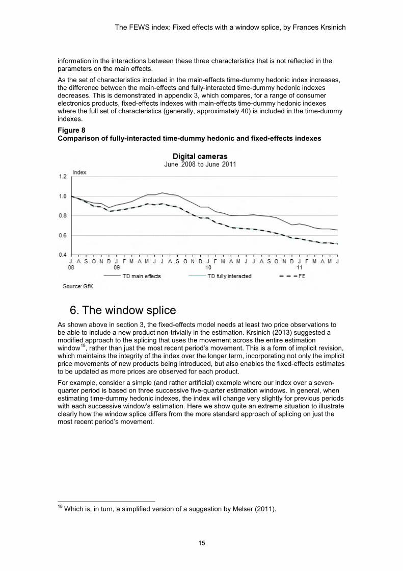
5. Simulation We use scanner data from market research company GfK for digital cameras, for the three years from July 2008 to June 201116. In order to run a fully-interacted time-dummy hedonic model, we incorporate just three of the approximately 40 available characteristics in the model. These are brand (with 22 categories), depth of device in millimetres (295 categories), and photos per second (78 categories). To estimate the corresponding fixed-effects index, we define product identifiers based on these three characteristics. For example: a product of brand A, with a depth of device in millimetres of 12, and photos per second of 100, could be assigned an identifier of ‘A_12_100’. A product of brand B, depth of device in millimetres of 25, and photos per second of 200, could be called ‘B_25_200’. Note that these product identifiers are text strings, and therefore convey no actual information about the corresponding characteristics to the estimation process17. Figure 8 shows the resulting indexes. The fully-interacted time-dummy hedonic index and the fixed-effects index are exactly the same. This is despite no characteristics being explicitly incorporated into the fixed-effects estimation. We also show the standard time-dummy hedonic index, which includes only the main effects of the three characteristics. The difference between this main-effects time-dummy hedonic index and the fully-interacted time-dummy hedonic index implies there is extra price-determining

16 The data is described in de Haan and Krsinich (2014a). 17 For example, we could rename them ‘Paul’ and ‘Mary’ and the estimation would be unaffected.

14


information in the interactions between these three characteristics that is not reflected in the parameters on the main effects. As the set of characteristics included in the main-effects time-dummy hedonic index increases, the difference between the main-effects and fully-interacted time-dummy hedonic indexes decreases. This is demonstrated in appendix 3, which compares, for a range of consumer electronics products, fixed-effects indexes with main-effects time-dummy hedonic indexes where the full set of characteristics (generally, approximately 40) is included in the time-dummy indexes.

Figure 8 Comparison of fully-interacted time-dummy hedonic and fixed-effects indexes

6. The window splice As shown above in section 3, the fixed-effects model needs at least two price observations to be able to include a new product non-trivially in the estimation. Krsinich (2013) suggested a modified approach to the splicing that uses the movement across the entire estimation window18, rather than just the most recent period’s movement. This is a form of implicit revision, which maintains the integrity of the index over the longer term, incorporating not only the implicit price movements of new products being introduced, but also enables the fixed-effects estimates to be updated as more prices are observed for each product. For example, consider a simple (and rather artificial) example where our index over a seven-quarter period is based on three successive five-quarter estimation windows. In general, when estimating time-dummy hedonic indexes, the index will change very slightly for previous periods with each successive window’s estimation. Here we show quite an extreme situation to illustrate clearly how the window splice differs from the more standard approach of splicing on just the most recent period’s movement.

18 Which is, in turn, a simplified version of a suggestion by Melser (2011).

15


Figure 9 Indexes estimated from three successive five-quarter windows

In this example, the index estimated from the first window has a constant increase of 10 percent per quarter, the index estimated on Window 2 is steeper, with a 15 percent per quarter increase each quarter, and Window 3’s index reflects a 20 percent increase in each quarter. The standard approach of splicing on the most recent period’s movement each time would result in an overall index showing a 10 percent increase each quarter from Y1Q1 to Y2Q1, then 15 percent from Y2Q1 to Y2Q2, and 20 percent from Y2Q2 to Y2Q3. This is shown in figure 10.

Figure 10 Splicing on the most recent period’s movement

The problem with this approach, however, is that the revised movement for back periods is not being incorporated into the longer-term index movement. Over time there will be a corresponding bias, which we could refer to as ‘splice drift’. Another approach to the splicing incorporates the movement across the entire window, so that the index always reflects the most up-to-date estimation of not only the most recent period’s movement, but the entire estimation window.

16


If we were able to revise the index, then this splicing of the most recent window’s index each time would look like that shown in figure 11. The revised index shows a 10 percent increase from Y1Q1 to Y1Q2, a 15 percent increase from Y1Q2 to Y1Q3, and 20 percent quarterly increases between Y1Q3 and Y2Q3. So, at all points the index is always based on the most recent estimation window possible.

Figure 11 Revising the index with the most recent window’s estimation

However, in production, we can’t revise the consumers price index. So the approach shown in figure 11 is not possible. Instead, we incorporate a ‘catch-up’ factor in the most recent period’s movement, to maintain the level of the index as it would be if we could revise. This is illustrated in figure 12.

Figure 12 Incorporating a window splice when the index can’t be revised

17


This approach trades off the quality of the most recent period’s estimated movement to improve the quality of the index over the longer term. And, in the case of fixed effects where at least two price observations are required before a new product contributes non-trivially to the estimation, this approach ensures there is no systematic bias due to the continual omission of the implicit price movements of new products entering the index. It does this by incorporating a revision for them in the period after their introduction (and also implicit revisions for the improvement of their fixed-effects estimates with more price observations). So, the published, and unrevisable, quarter’s movement incorporates a revision factor that adjusts the index to its value if we were able to revise. Obviously with such an artificial example as this, where the estimated index is changing significantly with each successive window’s estimation, the effect on the most recent period’s movement is quite substantial. But in practice the change to previous periods’ movements with the addition of one period of data is usually very small, so there would not be such a sacrifice in the quality of the most recent period’s movement to maintain an unbiased long-term index. The FEWS index combines this window-splice with the fixed-effects index, to produce both fully-quality-adjusted and non-revisable price indexes. Note that the implicit price movement from t-1 to t of a new product at time t won’t be reflected at time t until the window splice is incorporated for the index estimated at time t+1. That is, the implicit price movements will be reflected in the appropriate period, but with one period’s lag.

7. Empirical results We show empirical results for the FEWS index, on a range of data sources with different features:

• Scanner data from market research company GfK. Three years of monthly average prices with a full set of characteristics, and their associated quantities, for eight consumer electronics products in New Zealand.

• Scanner data from market research company IRI. Six years of monthly average prices for 30 supermarket products in the United States. This data has little information on characteristics of products but it does have quantities.

• Online data from the Billion Prices Project at MIT. Fifteen months of daily web-scraped online data for four consumer electronics products in New Zealand. This data has little information on characteristics of products, and no quantity information.

7.1 Scanner data with both quantities and characteristics: Eight New Zealand consumer electronics products First we produce the FEWS index on three years of monthly average prices from scanner data for New Zealand consumer electronics products, from market research company GfK. This data has extensive information on characteristics (around 40 different characteristics for each product) with corresponding total prices and quantities. From this we can derive average monthly prices and expenditures for each combination of characteristics. Because there is a full set of characteristics and expenditure information in the data, we can compare the FEWS index (which doesn’t require information on characteristics, only the product identifiers) with the imputation Tornqvist RYGEKS (ITRYGEKS) of de Haan and Krsinich (2014a). The ITRYGEKS index quality-adjusts for new and disappearing products appropriately, based on bilateral time-dummy hedonic indexes19.

19 This comparison has been made before, in Krsinich (2013). At that time, the FEWS index was referred to as the RY’TPD, to denote the rolling year time-product dummy index with a modified splice. While the FEWS, or RY’TPD, index performed well against the ITRYGEKS, it was not as close as in this paper. This was because not all the information in the data was being incorporated into the product identifier. The GfK output system has some aggregation for confidentiality, where the brand and/or model information is overwritten with a ‘tradebrand’

18


We also include the rolling year GEKS (RYGEKS) index of Ivancic, Diewert, and Fox (2011).

Figure 13 The FEWS index compared with RYGEKS and ITRYGEKS

identifier for some brands and/or models. In Krsinich (2013) the product identifier was based directly on the brand and model identifiers in the data, while the product identifier used for this analysis disaggregated the ‘tradebrand’ models to reflect different combinations of characteristics in the data.

19


For all products other than digital cameras, DVD players and recorders, and microwaves, the FEWS index sits closer to the ITRYGEKS than does the RYGEKS by the end of the three-year period. The RYGEKS tends to sit above the FEWS and ITRYGEKS indexes. The only exceptions to this are DVD players and recorders, and microwaves. The RYGEKS also tends to be more volatile than either of the FEWS or ITRYGEKS indexes. The difference between the RYGEKS and the FEWS reflects two factors. Firstly, the RYGEKS does not include the implicit price movements of new products entering into, and old products disappearing from, the market. As explained in section 3, the fixed-effects, and therefore the FEWS, index appropriately estimates the fixed effect for the new product such that, after two price observations, it is being appropriately incorporated into the estimation. The second factor appears not to have been recognised before now in the literature. The RYGEKS index is very sensitive to window length20. In the case of the eight consumer electronics products for which we have scanner data from GfK, the longer the window length, the flatter the GEKS21 index. Appendix 2 shows the effect of gradually increasing the window length for both fixed-effects and GEKS indexes, for two consumer electronics products. More research would be required to determine why the GEKS index behaves this way, and whether the effect is always a flattening or whether, for products with quality-adjusted price increases, the GEKS index steepens with increased window length. Our hypothesis is that the index estimation done by the GEKS procedure is equally weighting all bilateral periods across the full estimation window, while regression-based approaches such as the time-dummy hedonic or fixed-effects indexes implicitly put more weight on the data closer to the index movement being estimated. However, since we are likely to use a FEWS index rather than a RYGEKS index for data with no characteristics, understanding this issue is not a current research focus for Statistics NZ. What it means is the difference between the RYGEKS and indexes that incorporate the price movements of new and disappearing products, such as the ITRYGEKS, the RYTD, or the FEWS, shouldn’t be interpreted as only relating to the appropriate incorporation of the new and disappearing products. It is also being driven by this sensitivity to the window length of the RYGEKS.

7.2 Scanner data with quantities but no characteristics: 30 United States supermarket products Unlike the consumer electronics scanner data from GfK, supermarket scanner data tends to contain few characteristics with which to run either the ITRYGEKS or the rolling year time-dummy hedonic (RYTD) methods, which rely on hedonic models that explicitly incorporate a full set of price-determining characteristics. Other than the FEWS index, feasible methods, given the lack of information on characteristics, are chained superlative indexes and the RYGEKS index. Chained superlative indexes, for example the chained Tornqvist, can exhibit chain-drift as a consequence of the ‘spiking’ behaviour of prices and quantities due to sales. The RYGEKS is free of chain-drift, but does not reflect the implicit price movements associated with new and disappearing products.

20 We discovered this when comparing pooled GEKS-Jevons and FE indexes on the BPP online data. Initially, with eight months of data, these were relatively similar. When we obtained a longer 15-month period of data, the pooled GEKS-Jevons and FE indexes diverged significantly. 21 We looked at the building blocks of the RYGEKS index – the GEKS indexes – on different window lengths.

20


Figure 14 compares the FEWS index with both the chained-Tornqvist and the RYGEKS indexes for 30 supermarket products in the US, using research scanner data from IRI. Although weekly data is available, we used monthly average prices to calculate the monthly indexes for this paper, as the processing time to run six-year-long weekly indexes for 30 products was prohibitive.

Figure 14 The FEWS index compared with chained-Tornqvist and RYGEKS indexes

21


22


23


Perhaps the most striking feature of the results shown in figure 14 is that the three indexes are remarkably similar across the six years, for all 30 products, with just a few exceptions: facial tissues, paper towels, and razors, where the indexes diverge towards the end of the six-year period. For all three of these products, the RYGEKS and FEWS indexes are still quite similar to one another, with the chained Tornqvist diverging more strongly. It seems likely that the chained Tornqvist is generally not exhibiting chain-drift on these products because of the aggregation to monthly prices. This level of aggregation is likely to smooth out most of the spiking of prices and quantities we would see in daily average prices and, to a lesser extent, in weekly average prices. Taking the FEWS index as our fully-quality adjusted benchmark index, the RYGEKS appears not to be being biased by either the new / disappearing product’s implicit price movements not being incorporated, or by the GEKS index’s sensitivity to window length. This is in contrast to the results for consumer electronics products shown in section 7.1. Of course, we sacrifice some accuracy by using monthly averages rather than weekly averages – we are not reflecting compositional shifts within the month. A better estimation of the indexes would be to produce weekly indexes from the weekly average prices available in the data, and derive the monthly indexes (if monthly indexes are required in production) from these indexes. The reason for using monthly average prices here was the processing time required to run six years of weekly indexes for all 30 products. Further research could very usefully be done on this data. The generally very-close correspondence of the RYGEKS and the FEWS index for these products suggests the implicit price movements of products entering and leaving the market are very close to those of the matched products in the corresponding months. These results provide some reassurance that, for supermarket products, matched-model indexes such as the chained Tornqvist and RYGEKS may more appropriate than they have been shown to be for consumer electronics products (de Haan and Krsinich, 2014a). However, a comparison to monthly indexes derived from weekly indexes based on the weekly average prices would be desirable.

Also, understanding what drives the divergences in the indexes for facial tissues, paper towels, and razors is important.

7.3 Online data with no quantities or characteristics: four New Zealand consumer electronics products Statistics NZ was fortunate to be given access to 15 months of daily web-scraped online data from the Billion Prices Project at MIT, for New Zealand consumer electronics products. There are very few characteristics available in the online data but, as with scanner data, the products are identified by model name, and therefore any change in characteristics will have a different product identifier. This means that the fixed-effects index can be used to implicitly quality-adjust for all price-determining characteristics.

24


Another limitation of online data is that quantities are not available. The method used by the Billion Prices Project (and the inflation indicators of PriceStats) is a daily-chained Jevons. For the initial analyses shown here, we used day-per-week (Saturday) samples of the daily data. We did this because the processing time for calculating GEKS indexes on a year22 of daily data was too long. Figure 15 compares the weekly-chained Jevons with a RYGEKS index (based on bilateral Jevons indexes) and the (unweighted) fixed-effects index. Note that, because our estimation is not much longer than a year (the standard window length) we have simplified the index calculations slightly. For the RYGEKS, we calculated two year-long GEKS indexes and linked them together at the midpoint of the 15-month period. We denote this different approach by RY*GEKS rather than RYGEKS. And, rather than calculating a FEWS index, we calculated a fixed-effects index based on the pooled 15 months of data. We believe that the results will be very similar to both the RYGEKS and FEWS indexes, respectively. Note that there was a lapse in data collection for a couple of months from January 2013 to March 2013, which results in a flat index for each of the products over this period.

Figure 15 Fixed-effects indexes compared with RYGEKS and weekly-chained Jevons

Over the 15-month period, the three indexes are quite similar, with the exception of mobile computers, where the RY*GEKS index diverges from the other two methods near the start of the 15-month period, and digital cameras, where the chained Jevons has drifted away from the other two indexes by the end of the 15-month period. There is little evidence of chain-drift in the weekly-chained Jevons. This may be a consequence of the lack of quantities in the data, as it appears to be the slight asymmetry in the price and quantity spiking that drives chain-drift23. Cavallo (2012) discussed possible approaches to quality-adjusting the online data, which prompted this collaborative research into fixed-effects as an appropriate method for quality adjustment. These initial results suggest that the daily-chained Jevons may be doing a better

22 Actually, one year plus a day, so 366 days. 23 Though the author is not aware of whether this has been formally established anywhere in the literature.

25


job of quality adjustment than was assumed, given how close it sits to the fixed-effects index. In fact, our research into the fixed-effects index has clarified to us that the matched-model approaches are able to reflect new products being of a different quality to existing products. What they won’t do is appropriately reflect the implicit price movements of new and disappearing products if these differ from the price movements of the matched products in the corresponding period. Statistics NZ has recently entered into a research agreement with PriceStats, who will begin to collect and process online data for a wide range of New Zealand retailers, which we will use for research. In addition to further exploring the performance of the FEWS index in comparison with the current daily-chained Jevons index for online data, we will be able to compare the indexes derived from online data with those from scanner data for New Zealand consumer electronics products24.

8. Comparing methods A range of methods could be appropriate for producing non-revisable price indexes from scanner or online data, or in fact any other ‘big data’ on prices that has longitudinal price information at a detailed product level. This paper has described the fixed-effect window-splice (FEWS) index, and contrasted it with other indexes:

• a chained Tornqvist (or, in the case of the online data which lacks quantities, a chained Jevons)

• the rolling year GEKS (RYGEKS) • the rolling year time-dummy (RYTD) hedonic index25 • the imputation Tornqvist RYGEKS (ITRYGEKS).

Each of these methods differs in their data requirements, complexity, and performance. In figure 16, we classify each of the methods according to a range of criteria. We denote positive attributes of the indexes by a (+) and negative attributes by a (-). We shade the cells correspondingly, with dark shading for negative attributes and lighter shading for the neutral ‘maybe’ classifications. Depending on the situation, some of these criteria are far more important than others, so we don’t attempt to come up with any kind of summary measures across the criteria. According to this list of criteria, the only negative features of the FEWS index are:

• It requires statistical software. Specifically, the ability to estimate general linear models. This, however, is a feature shared by all the methods except the chained Tornqvist and the RYGEKS.

• It is not easy to explain. Over time, this may become less of an issue, as the method is more widely understood. Only recently have we come up with the intuitive visual explanation of section 3, which we hope will help make the method more understandable.

And we have given a ‘maybe’ ranking for the criteria ‘can be explicitly formulated in terms of index theory’. However, recent work by de Haan and Krsinich (2014b) shows that the time-dummy hedonic index is equivalent to a quality-adjusted unit value index (though using a geometric, rather than a harmonic, mean). Given the equivalence of the fixed-effects and the fully-interacted time-dummy hedonic index, we believe this ‘maybe’ could be changed to a ‘yes’– but at time of writing this is still an open question in the literature.

24 Statistics NZ intends to use GfK scanner data in production for consumer electronics from the September 2014 quarter, using the ITRYGEKS method. 25 Actually, we compare the pooled fixed-effects index to the pooled time-dummy hedonic index in appendix 3. For the purposes of the comparison in this section, though, we consider the non-revisable version of the time-dummy hedonic index, the rolling year time-dummy (RYTD).

26


Figure 16 Comparison of five different indexes

9. Conclusion We have shown in this paper – intuitively, theoretically, and empirically – that the fixed-effects window-splice (FEWS) index produces fully quality-adjusted non-revisable price indexes in the case of big data, such as scanner data or online data, where there is longitudinal price information at a detailed product-specification level. From the December 2013 quarter, Statistics NZ has incorporated fixed-effects indexes into production for mobile phones and televisions in the New Zealand import price index. We are likely to consider using FEWS indexes for supermarket products in the New Zealand consumers price index if we can get full-coverage scanner data from the major supermarket chains. We are also considering using the FEWS approach in the context of online data. We have recently entered into a research agreement with PriceStats, who will be providing us with monthly feeds of daily online data for a wide range of New Zealand online retailers, so we can research the potential of this approach. The estimation of FEWS indexes is very simple, as long as statistical software is available for estimating generalised linear models – appendix 3 provides the data structure and SAS code required to estimate the underlying fixed-effects indexes. In the course of the analysis on which this paper was based, some other findings have arisen, all of which could be usefully researched further.

• The GEKS index (and possibly, though likely to a much lesser extent, the ITRYGEKS index26) is very sensitive to window length.

• The monthly chained-Tornqvist index, when derived from monthly average prices, appears not to suffer from chain-drift in the context of scanner data on US supermarket products.

• The FEWS index may not work in the case of products where the start and end dates of product life cycles are highly seasonal – for example, women’s clothing. If so, there may be a requirement to have at least some minimum proportion of product specifications matched and not in a state of end-of-line discounting, between each pair of successive periods for the FEWS index to be successfully estimated.

Appendix 1: Derivation of equation 4 Restating and extending the working of de Haan and Hendriks (2013) so that all characteristics are treated as categorical and all interactions are included in the time-dummy hedonic models along with the main effects, the predicted prices of item (ie product specification) i in the base period 0 and the comparison periods t are as follows.

26 We tested the effect of window length on the ITRYGEKS index for laptop computers, which was virtually unaffected by changes to the window length. However, this may not be representative of the behaviour of other products.

27


+= ∑ ∑

= =

L

l

M

mimmilli DzDp

1 1

00 ˆêxp)êxp(ˆ ββδ (6)

+= ∑ ∑

= =

L

l

M

mimmill

tti DDp

1 1

0 ˆêxp)êxp()êxp(ˆ ββδδ; (t=1,…,T) (7)

Taking the geometric mean of the predicted prices for all items belonging to the samples 0S

and TSS ,...,1

gives the following.

+= ∑ ∑ ∑ ∑∏

= ∈ = ∈∈

L

l Si

M

m Siimmill

Si

Ni NDDp

1

0

1

01

0

0 00

0 /)ˆˆ(exp)êxp()ˆ( ββδ (8)

+= ∑ ∑ ∑ ∑∏

= ∈ = ∈∈

L

l Si

tM

m Siimmill

t

Si

Nti

t tt

t NDDp1 1

01

/)ˆˆ(exp)êxp()êxp()ˆ( ββδδ; (t=1,…,T) (9)

Dividing (9) by (8) and rearranging gives the following.

+

+

=

∑ ∑ ∑ ∑

∑ ∑ ∑ ∑

∏

∏

= ∈ = ∈

= ∈ = ∈

∈

∈L

l Si

tM

m Siimmill

L

l Si

M

m Siimmill

Si

Ni

Si

Nti

t

t t

t

t

NDD

NDD

p

p

1 1

1

0

11

0

1

/)ˆˆ(exp

/)ˆˆ(exp

)ˆ(

)ˆ()êxp(

0 0

0

0 ββ

ββδ

−+−= ∑ ∑

∏

∏= =

∈

∈L

l

M

m

tmmm

tlll

Si

Ni

Si

Nti

DDDDp

pt

t

1 1

001

0

1

)(ˆ)(êxp)ˆ(

)ˆ(

0

0

ββ

(10)

Where 0

0 0

N

DD Si

il

l

∑∈= and

t

Siil

tl N

DD t

∑∈= are the unweighted sample means of the dummy

variable for category l of the main effects and 0

0 0

N

DD Si

im

m

∑∈= and

t

Siim

tm N

DD t

∑∈= are the

unweighted sample means of the dummy variable for category m of the second-order interactions. Because the residual terms sum to zero in each period, (10) can be rewritten.

−+−== ∑ ∑

∏

∏= =

∈

∈L

l

M

m

tmmm

tlll

Si

Ni

Si

Nti

ttTD DDDD

p

pP

t

t

full1 1

001

0

1

0 )(ˆ)(êxp)(

)()êxp(

0

0

ββδ

; (t=1,…,T) (11)

28


And this is equation (4) in the main text.

Appendix 2: Sensitivity to window length As noted in section 7.1, the GEKS index is very sensitive to the length of the estimation window. We investigated this across all eight consumer products for which we have scanner data from market research company GfK. Figure 17 shows the effect of estimating pooled fixed-effects and GEKS indexes, on gradually increasing windows of data, from six months, for desktop computers and televisions27. We base the index at the midpoint of the three-year period – January 2010 – and centre the gradually increasing estimation windows about this point. Note that the GEKS index is undefined beyond 18 months for desktop computers, and 30 months for televisions. This is because, beyond these window lengths, there are some pairs of months where there are no matched product specifications from which to calculate the required Tornqvist indexes. We include the time-dummy hedonic index as a benchmark in both the graphs. As you can see, the fixed-effects indexes on the gradually increasing window lengths tend to converge to the time-dummy hedonic index, while the GEKS indexes flatten significantly as the window lengths increase. This appears to be quite a significant form of biasing in the GEKS indexes, which would make the definition of window length very important for the RYGEKS index. As noted above, this issue requires further research, and appears to be an important consideration for any statistical office intending to use the RYGEKS in production. Having said that, the results shown in section 7.3 for supermarket products suggest they might be less significantly affected by window length than consumer electronics products are.

27 The corresponding graphs for the other six consumer electronics products show similar patterns, and can be obtained on request from the author.

29


Figure 17 The effect of different window lengths on fixed-effects and GEKS indexes

Appendix 3: Comparison of pooled fixed-effects, time-dummy hedonic, and GEKS indexes Having noted in appendix 2 the sensitivity of the GEKS index to window length, we now present results comparing pooled indexes on the maximum length of window for which GEKS are defined. We compare GEKS, main-effects time-dummy hedonic, and fixed-effects indexes. These demonstrate clearly how closely the fixed-effects and time-dummy hedonic indexes compare, even though these time-dummy hedonic indexes incorporate main-effects only. As noted in section 5, an increasing set of characteristics included in the main-effects time-dummy hedonic index causes it to converge to the fully-interacted time-dummy hedonic index, which we have shown is equivalent to the fixed-effects index.

30


Figure 18 Pooled fixed-effects indexes, compared with pooled GEKS and time-dummy hedonic indexes

For all products except two – DVD players and recorders, and portable media players – the main-effects time-dummy hedonic indexes and the fixed-effects indexes are virtually identical. As noted above, this makes sense because with such a large set of characteristics, we wouldn’t expect much extra price-determining information to be picked up by interactions between the characteristics. Therefore the main-effects time-dummy hedonic indexes should be very similar to the fully-interacted time-dummy hedonic indexes.

31


For those products where the main-effects time-dummy hedonic index and the fixed-effects index do diverge slightly – DVD players and recorders, and portable media players – this divergence is due to one or both of two factors:

• interactions between the characteristics contain extra price-determining information • there are some unmeasured characteristics not fully correlated with one or a

combination of measured characteristics, which will be reflected by the fixed-effects index but not the time-dummy index.

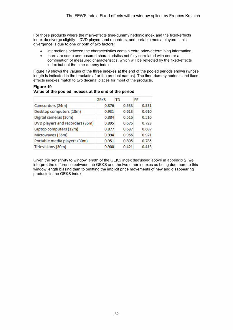
Figure 19 shows the values of the three indexes at the end of the pooled periods shown (whose length is indicated in the brackets after the product names). The time-dummy hedonic and fixed-effects indexes match to two decimal places for most of the products.

Figure 19 Value of the pooled indexes at the end of the period

Given the sensitivity to window length of the GEKS index discussed above in appendix 2, we interpret the difference between the GEKS and the two other indexes as being due more to this window length biasing than to omitting the implicit price movements of new and disappearing products in the GEKS index.

32


Appendix 4: Data structure and SAS code to produce the fixed-effects index The fixed-effects index is very easy to estimate, with statistical software such as SAS/Stat. Figure 20 shows the data structure required for the window of time being estimated – generally this will be one year plus a period (ie five quarters, or 13 months, or 53 weeks).

Figure 20 Data structure for estimating fixed-effects index

The SAS code for running the fixed-effects model on this pooled 13-month data is as follows.

ods output parameterestimates=FE_parameters fitstatistics= FE_fit; proc glm data=product_data; absorb product_spec_id; class month; model log_av_price = month / solution; weight exp_share; run; And the index for month t is derived from the parameters estimated for each month as

)exp(/)exp( 0ββ t .

Note that the ‘absorb’ statement is telling SAS to fit product_spec_id-specific intercepts, without outputting all the associated parameters. The same model would be estimated if this statement was left out, and product_spec_id was included in the class and model statements instead. In production, the 13-month pooled fixed-effects index would be run on the data up to and including the most recent month’s data, and the published index would be that resulting from splicing on the movement across the full 13-month estimation window as shown in section 6. SAS code to run the FEWS index retrospectively across a longer period than 13 months – that is, running the fixed-effects index on successive 13-month windows of data and appropriately splicing in the full window’s movement for each period – can be obtained on request from the author. We’re very interested in others’ experiences running the FEWS index on different data sources.

33


References Aizcorbe, A, Corrado, C, & Doms, M (2003). When do matched-model and hedonic techniques yield similar price measures? Working Paper no. 2003-14, Federal Reserve Bank of San Francisco.

Allison, PD (2005). Fixed-effects regression methods for longitudinal data using SAS. Cary, NC: SAS Institute Inc.

Cavallo, A (2012). Overlapping quality adjustment using online data. Paper presented at the 2012 Economic Measurement Group, Sydney, Australia. November 2012.

de Haan, J, & Hendriks, R (2013, November). Online data, fixed effects and the construction of high-frequency price indexes. Paper presented at the 2013 Economic Measurement Group, Sydney, Australia. de Haan, J, & Krsinich, F (2014a). Scanner data and the treatment of quality change in non-revisable price indexes. Journal of Business & Economic Statistics (forthcoming). de Haan, J, & Krsinich, F (2014b, August). Time-dummy hedonic and quality-adjusted unit value indexes: Do they really differ? Paper to be presented at the conference of the Society for Economic Measurement, Chicago. Diewert, WE (2004). On the stochastic approach to linking the regions in the ICP. Discussion Paper no. 04-16, Department of Economics, University of British Columbia, Vancouver, Canada. Ivancic, L, Diewert, WE, & Fox, KJ (2011). Scanner data, time aggregation and the construction of price indexes. Journal of Econometrics, 161(1), 24–35. Krsinich, F (2011, May). Measuring the price movements of used cars and residential rents in the New Zealand consumers price index. Paper presented at the 12th meeting of the Ottawa Group, Wellington, New Zealand.

Krsinich, F (2013, May). Using the rolling year time-product dummy method for quality adjustment in the case of unobserved characteristics. Paper presented at the 13th meeting of the Ottawa Group, Copenhagen. Melser, D (2011, May). Constructing cost of living indexes using scanner data, unpublished draft, September 2011 – an updated version of Constructing high frequency indexes using scanner data, paper presented at the 12th meeting of the Ottawa Group, Wellington, New Zealand.

34

the fews index: fixed effects with a window · pdf filethe fews index: fixed effects with a...

Documents