the effects of tourism impacts upon - virginia tech
TRANSCRIPT
THE EFFECTS OF TOURISM IMPACTS UPON QUALITY OF LIFE OF RESIDENTS IN THE COMMUNITY
By
Kyungmi Kim
Dissertation submitted to the Faculty of the Virginia Polytechnic Institute and State University
In partial fulfillment of the requirements for the degree of
DOCTOR OF PHILOSOPHY
In
Hospitality and Tourism Management
APPROVED:
____________________________________ Muzaffer Uysal, Chairman
_________________________________ ___________________________________ Ken McCleary M. Joseph Sirgy
________________________________ __________________________________ Susan Hutchinson Joseph Chen
November 5, 2002 Blacksburg, Virginia
Keywords: Perceptions, Tourism Impacts, Development Cycle and Quality of Life
Copyright 2002, Kyungmi Kim
The effects of tourism impacts upon Quality of Life of residents in the community
Kyungmi Kim Committee Chair: Muzaffer Uysal
Department of Hospitality and Tourism Management
ABSTRACT
This study investigates how tourism affects the quality of life (QOL) of residents in tourism destinations that vary in the stage of development. The proposed model in this study structurally depicts that satisfaction with life in general derives from the satisfaction with particular life domains. Overall life satisfaction is derived from material well-being, which includes the consumer’s sense of well being as it is related to material possessions, community well-being, emotional well-being, and health and safety well-being domains. The model also posits that residents’ perception of tourism impacts (economic, social, cultural, and environmental) affects their satisfaction of particular life domains. Lastly, this study investigates that tourism development stages moderate the relationship between residents’ perception of tourism impacts and their satisfaction with particular life domains. Accordingly, the study proposed four major hypotheses: (1) residents’ perception of tourism impacts affects their QOL in the community, (2) residents’ satisfaction with particular life domains is affected by the perception of particular tourism impact dimensions, (3) residents’ satisfaction with particular life domains affects residents’ life satisfaction in general, and (4) the relationship between residents’ perception of tourism impacts and their satisfaction with particulate life domains is moderated by tourism development stages. The sample population consisting of residents residing in Virginia was surveyed. The sample was proportionally stratified on the basis of tourism development stages covering counties and cities in the state. Three hundred and twenty-one respondents completed the survey. Structural Equation Modeling and Hierarchical Multiple Regression were used to test study hypotheses.
The results revealed that the residents’ perception of tourism impacts did affect their satisfaction with particular life domains significantly, and their satisfaction with particular life domains influenced their overall life satisfaction. The hypothesized moderating effect of tourism development stages on the relationship between the perception of tourism impacts and the satisfaction with particular life domains was not supported. The results indicated that the relationship between the economic impact of tourism and the satisfaction with material well-being, and the relationship between the social impact of tourism and the satisfaction with community well-being were strongest among residents in communities characterized to be in the maturity stage of tourism development. This finding is consistent with social disruption theory which postulates that boomtown communities initially enter into a period of generalized crisis, resulting from the traditional stress of sudden, dramatic increases in demand for public services

and improving community infrastructure (England and Albrecht’s (1984). Additionally, residents develop adaptive behaviors that reduce their individual exposure to stressful situations. Through this process, the QOL of residents is expected to initially decline, and then improve as the community and its residents adapt to the new situation (Krannich, Berry & Greider, 1989). However, when a community enters into the decline stage of tourism development, the relationship between the economic impact of tourism and the satisfaction with material well-being, and the relationship between the social impact of tourism and the satisfaction with community well-being may be considered to be the capacity of the destination area to absorb tourists before the host population would feel negative impacts. This is consistent with the theoretical foundation of carrying capacity, suggesting that when tourism reaches its maturity or maximum limit, residents’ QOL may start deteriorating.
Further, the relationship between the cultural impact of tourism and the
satisfaction with emotional well-being, and the relationship between the environmental impact of tourism and the satisfaction with health and safety well-being were strongest in the decline stage of tourism development. Neither the theories of social carrying capacity nor social disruption offered much to explain this result. However, this result is consistent with Butler’s (1980) argument that in the decline stage, more tourist facilities disappear as the area becomes less attractive to tourists and the viability of existing tourist facilities becomes more available to residents in the destination community. As residents’ perception of negative environmental impacts increases, their satisfaction with health and safety well-being decreases in the decline stage of tourism development unless the area as a destination provides rejuvenating or alternative planning options.
It has been well established that residents in certain types of tourism communities might perceive a certain type of tourism impact unacceptable, while in other communities, the same impact type may be more acceptable. Thus, the study suggests that the proposed model should be further tested and verified using longitudinal data.
To My Loving Parents
But when perfection comes, the imperfect disappears. When I was a child, I talked
like a child, I thought like a child, I reasoned like a child. When I became a man, I put childish ways behind me. Now we see but a poor reflection as in a mirror; then we shall see face to face. Now I know in part; then I shall know fully, even as I am fully known. And now these three remain: faith, hope and love. But the greatest of these is love.
- Corinthians I: 13:10-13 -
iv
ACKNOWLEDGEMENT A project of this magnitude is not an individual endeavor. Consequently, I dedicate this dissertation to the many individuals who provided support, encouragement and assistance for its realization. A very special gratitude goes to my committee members, Dr. Muzaffer Uysal, Dr. Ken McCleary, Dr. Joseph Sirgy, Dr. Susan Hutchinson and Dr. Joseph Chen, for their support and input. Dr. Muzaffer Uysal, committee Chairman, has been an inspiration and a mentor for me throughout my doctoral pursuit. I am sincerely grateful for the research opportunities he afforded me. Particularly valued are his accessibility, the breadth and depth of his knowledge, and his ability to instill confidence. In particular, his unique way of encouraging me with research opportunities and praise has benefited me greatly and has guided me in the accomplishment of my dissertation. For helping me stretch and reach for the best, I am grateful to Dr. Joseph M. Sirgy. His expansive knowledge and firm commitment to supporting this work have set high standards, which allowed me to explore and discover on my own. And also the gift he offered me was the inspiration to be all that I could be, to reach beyond what is acceptable to what is excellent.
I wish to thank Dr. Ken McCleary for his assistance in elucidating the research question, and resecifying unclear location and inconsistence. His cheerful nature of expansive knowledge and academic diligence are highly valued.
Dr. Susan Hutchinson’s gift of making students feel comfortable asking question is especially appreciated. Her probing question was helpful in discerning the precepts underlying my research in statistical area. Gratitude is expressed for her sincerely and sagacity.
I would like to thank you Dr. Joseph Chen for offering many insight and keen questions and that contributed to this study and for showing me kindness when I needed it most. I am grateful to the National Tourism Foundation, which awarded me a “Luray Caverns Graduate Research Grant”. Without this grant, I could not be able to finish the survey of my study. Last, but not least, I am grateful to my mother, Byungrae L. Kim, for having always emotionally supported my academic endeavors. I wish to thank my father, Wonsang, who showed me his love and passion for education. I would like to thank my sisters, Kyunghwa and Kyungae, and my brothers, Eungsun and Eungsoo, for their love, support and patience.
v

TABLE OF CONTENTS
CHAPTER ONE: INTRODUCTION
1.1 Introduction --------------------------------------------------------------------- 1 1.2 Research questions --------------------------------------------------------------------- 1 1.3 Knowledge of foundation ------------------------------------------------------------- 6 1.4 Objectives ------------------------------------------------------------------------------ 8 1.5 Theoretical basis ----------------------------------------------------------------------- 9 1.6 Propositions ----------------------------------------------------------------------------- 15 1.7 Structural model of the study -------------------------------------------------------- 20 1.8 Contribution of the study ------------------------------------------------------------ 21 1.8.1 Theoretical advancement in tourism study ----------------------------- 21 1.8.2 Practical application for the tourism-planning program -------------- 21 1.9 Chapter summary----------------------------------------------------------------------- 22
CHAPTER TWO: LITERATURE REVIEW
2.1 Introduction ---------------------------------------------------------------------------- 23 2.2 Relevance of the research ----------------------------------------------------------- 23 2.3 Tourism impacts ---------------------------------------------------------------------- 25
2.3.1 Economic impacts --------------------------------------------------- ------- 27 Employment opportunities --------------------------------------------- 26 Revenues from tourists for local business and standard for living - 29
Cost of living -------------------------------------------------------------- 29 2.3.2 Social impacts --------------------------------------------------------------- 30 Congestion ----------------------------------------------------------------- 31 Local service --------------------------------------------------------------- 31
Increasing social problem ------------------------------------------------ 32 2.3.3 Cultural impacts ------------------------------------------------------------- 32 Preservation of local culture --------------------------------------------- 33 Cultural exchanges between residents and tourists ------------------- 34 2.3.4 Environmental impacts ----------------------------------------------------- 35 Pollution -------------------------------------------------------------------- 35 Solid waste ----------------------------------------------------------------- 36 Wildlife --------------------------------------------------------------------- 36
2.3.5 Social carrying capacity ---------------------------------------------------- 39 2.3.6 Life cycle model ------------------------------------------------------------- 40
2.3.6.1 Beginning stage --------------------------------------------------- 44 2.3.6.2 Growth stage ------------------------------------------------------ 44
2.3.6.3 Maturity stage ----------------------------------------------------- 45 2.3.6.4 Decline stage ------------------------------------------------------ 46
2.4 Quality of life studies ------------------------------------------------------------------ 47 2.4.1 Material well-being domain ------------------------------------------------ 54 Standard of living ---------------------------------------------------------- 54 Income and employment -------------------------------------------------- 55
vi

2.4.2 Community well-being domain ------------------------------------------- 57 2.4.3 Emotional well-being domain --------------------------------------------- 58 Leisure activity ------------------------------------------------------------- 58 Spiritual activity ----------------------------------------------------------- 60 2.4.4 Health and safety well-being domain ------------------------------------- 61 2.4.5 Other well-being domains -------------------------------------------------- 62 Family well-being --------------------------------------------------------- 62 Neighborhood well-being ------------------------------------------------- 63 2.5 Chapter summary ------------------------------------------------------------------------ 64 CHAPTER THREE: RESEARCH METHODOLOGY 3.1 Introduction ----------------------------------------------------------------------------- 65 3.2 Research framework ------------------------------------------------------------------ 65 3.3 Research hypotheses ------------------------------------------------------------------ 67 3.4 Statistical method employed --------------------------------------------------------- 69 3.4.1 Phase I: Structural equation model--------------------------------------- 69 3.4.1.1 Measurement model --------------------------------------------- 69 3.4.1.2 Structural equation model --------------------------------------- 71 3.4.2 Phase II: Hierarchical multiple regression ------------------------------- 73 3.5 Research design ------------------------------------------------------------------------ 74 3.5.1 Survey instrument ---------------------------------------------------------- 74 3.5.2 Data collection -------------------------------------------------------------- 74 3.5.3 Sample ------------------------------------------------------------------------ 74 Stratified random sampling ---------------------------------------------- 75 Sample size ----------------------------------------------------------------- 81 3.5.4 Measurement variables ----------------------------------------------------- 81 3.5.4.1 Exogenous variables --------------------------------------------- 82 Economic impact variables -------------------------------------- 83 Social impact variables ------------------------------------------ 84 Cultural impact variables ---------------------------------------- 85 Environmental impact variables -------------------------------- 86 3.5.4.2 Endogenous variables ------------------------------------------- 87 Material well-being variables ---------------------------------- 87 Community well-being variables ------------------------------ 88 Emotional well-being variables -------------------------------- 88 Health and Safety variables ------------------------------------ 89 QOL in general --------------------------------------------------- 90 3.5.5 Pretest of the measurement instrument ---------------------------------- 91 3.6 Reliability and validity ---------------------------------------------------------------- 91 3.7 Chapter summary ----------------------------------------------------------------------- 93 CHAPTER FOUR: ANALYSIS AND RESULTS 4.1 Introduction ------------------------------------------------------------------------------ 94 4.2 Pretest ------------------------------------------------------------------------------------ 94
vii
4.2.1 Pretest Survey method --------------------------------------------------- 95 4.2.2 Pretest sample ------------------------------------------------------------- 96 4.2.3 Results from the pretest --------------------------------------------------- 97 4.2.3.1 Economic impact variable ------------------------------------ 98 4.2.3.2 Social impact variables ---------------------------------------- 101 4.2.3.3 Cultural impact of tourism variables ------------------------- 103 4.2.3.4 Environmental impact of tourism variables ---------------- 105 4.2.3.5 Material well-being domain ----------------------------------- 106 4.2.3.6 Community well-being domain ------------------------------ 108 4.2.3.7 Emotional well-being domain -------------------------------- 109 4.2.3.8 Health and safety well-being domain ------------------------ 110 4.2.3.9 Quality of life (QOL) in general ------------------------------ 112 4.3 Final survey ----------------------------------------------------------------------------- 113 4.3.1 Survey method -------------------------------------------------------------- 113 4.3.2 Samples ---------------------------------------------------------------------- 114 4.3.3 Profile of the respondents ------------------------------------------------- 115 4.3.4 Late-response Bias Tests -------------------------------------------------- 117 4.3.5 Descriptive statistics, Skewness, and Kurtosis ------------------------- 118 4.4 Data analysis ---------------------------------------------------------------------------- 119 4.4.1 Confirmatory factor analysis (CFA) ------------------------------------ 119 4.4.1.1 CFA of economic impact of tourism constructs ------------- 121 4.4.1.2 CFA of social impact of tourism constructs ------------------ 123 4.4.1.3 CFA of cultural impact of tourism constructs ---------------- 124 4.4.1.4 CFA of the environmental impact of tourism construct ---- 126 4.4.1.5 CFA of the material well-being construct -------------------- 127 4.4.1.6 CFA of the community well-being construct ---------------- 129 4.4.1.7 CFA of the emotional well-being constructs ----------------- 130 4.4.1.8 CFA of the health and safety well-being construct ---------- 131 4.4.2 Testing the proposed model ------------------------------------------------ 133 4.4.2.1 Measurement model --------------------------------------------- 134 4.4.2.2 Fit indices --------------------------------------------------------- 143 4.4.2.3 Discriminality validity ------------------------------------------- 147 4.4.2.4 Convergent validity ---------------------------------------------- 150 4.4.2.5 Testing the proposed model and hypotheses ----------------- 150
4.4.2.5.1 Testing the hypothesized structural model ------- 156 4.4.2.5.2 Analysis of the Hypotheses ------------------------- 161
4.4.2.6 Testing of moderating effects ---------------------------------- 166 4.5 Chapter summary ----------------------------------------------------------------------- 190 CHAPTER V: DISCUSSION AND CONCLUSION
5.1 Introduction ----------------------------------------------------------------------------- 194 5.2 Summary of findings ------------------------------------------------------------------ 194 5.3 Discussions of the findings ------------------------------------------------------------ 196
5.3.1 Research questions and hypotheses -------------------------------------- 199 5.3.2 Summary of the discussion ------------------------------------------------ 210
5.4 Implication of this study -------------------------------------------------------------- 210
viii
5.4.1 Managerial implications --------------------------------------------------- 210 5.4.2 Theoretical implications --------------------------------------------------- 213 5.5 Limitations of the study --------------------------------------------------------------- 215 5.6 Suggestions of the future study ------------------------------------------------------ 216 5.7 Conclusions ----------------------------------------------------------------------------- 217 REFERENCES ----------------------------------------------------------------------- 219 APPENDIX A. Survey Instrument ---------------------------------------------- 236 APPENDIX B. Reminder postcard ---------------------------------------------- 245 APPENDIX C. Counties and cities in each stage and the number of
respondents from each county and city ------------------------ 246
APPENDIX D. Demographic Profile of the respondents --------------------- 247 APPENDIX E. The results of the Pearson Chi-Square test for late
response bias tests ----------------------------------------------- 250
APPENDIX F. Individual items of the constructs with mean scores and standard deviation ---------------------------------------------- 253
APPENDIX G. The procedure of selecting the number of indicators ------- 259
ix
LIST OF TABLES Table 2.1 The major positive and negative impacts of tourism ------------------ 38 Table 2.2 The characteristics of tourism development stage --------------------- 43 Table 3.1 The criterion of the development stage --------------------------------- 76 Table 3.2 The criterion of the development stage associated with indicators -- 78 Table 3.3 Counties and cities in each stage and the number of stratified
Sample ---------------------------------------------------------------------- 80 Table 4.1 Demographic Profile of the pretest sample -------------------------- 97 Table 4.2 Factor analysis result of the economic impact of tourism construct 100 Table 4.3 Factor analysis result of the social impact of tourism construct --- 102 Table 4.4 Factor analysis result of the cultural impact of tourism construct --- 104 Table 4.5 Factor analysis result of the environmental impact of tourism
Construct ------------------------------------------------------------------- 106 Table 4.6 Factor analysis result of material well-being construct --------------- 107
Table 4.7 Factor analysis result of community well-being construct ----------- 108
Table 4.8 Factor analysis result of emotional well-being construct ------------- 110 Table 4.9 Factor analysis result of health and safety well-being construct ---- 112
Table 4.10 Factor analysis result of the quality of life in general ---------------- 113
Table 4.11 Response Rate ------------------------------------------------------------ 114 Table 4.12 The result of the χ2 test for objective and subjective
development stage -------------------------------------------------------- 117 Table 4.13 Composite Reliability and validity of the economic impact variables
-------------------------------------------------------------------------------- 123 Table 4.14 Composite Reliability and validity of the social impact variables -- 125
x
Table 4.15 Composite Reliability and validity of the cultural impact variables -126 Table 4.16 Composite Reliability and validity of the environmental impact
Variables ---------------------------------------------------------------- 128 Table 4.17 Composite Reliability and validity of material well-being variables 129 Table 4.18 Composite Reliability and validity of the community well-being
Variables ------------------------------------------------------------------- 130 Table 4.19 Composite Reliability and validity of the emotional well-being
Variables ------------------------------------------------------------------ 131 Table 4.20 Composite Reliability and validity of the health and safety
well-being ----------------------------------------------------------------- 133 Table 4.21 Parameter estimates for the proposed nine-factor measurement
Model -------------------------------------------------------------------- 138 Table 4.22 Composite reliability and validity of overall measurement model - 141 Table 4.23 Fit indices the proposed measurement model ------------------------- 144 Table 4.24 Results of Discriminant Validity Tests --------------------------------- 149 Table 4.25 Fit indices for five sub-model ------------------------------------------- 154 Table 4.26 The results of SCDT ------------------------------------------------------ 155 Table 4.27 Pattern of estimated parameters in the Gamma and Beta matrices -- 158 Table 4.28 Fit-indices the proposed theoretical model ---------------------------- 159 Table 4.29 Estimated standized coefficients for the hypothesized model ------ 160 Table 4.30 Results of a Hierarchical MRC analysis for economic impact and
development stages ------------------------------------------------------- 169 Table 4.31 Results of a HMR analysis for economic impact and perceived
development stages ------------------------------------------------------- 173 Table 4.32 Results of a Hierarchical MRC analysis for social impact and
development stages ------------------------------------------------------ 175 Table 4.33 Results of a HMRC analysis for social impact and perception of
development stages ------------------------------------------------------ 178
xi
Table 4.34 Results of a Hierarchical MRC analysis for cultural impact
and development stages ------------------------------------------------ 181 Table 4.35 Results of a HMRC analysis for cultural impact and
the perception of the development -------------------------------------- 183 Table 4.36 Results of a HMRC analysis for environmental impact and
development stages ----------------------------------------------------- 186 Table 4.37 Results of a HMRC analysis for environmental impact and
perception of the development ---------------------------------------- 188 Table 4.38 The summary of hypotheses testing results ------------------------- 190 Table 5.1 Hypothesized relationships and results ------------------------------- 199
xii
LIST OF FIGURES
Figure 1.1 The relationships among perceived tourism impacts, development stage, particular life domains, and quality of life ----- 8
Figure 1.2 Tourism exchange system modified from Jurowski, 1994 ----------- 14 Figure 1.3 Tourism impacts model of the quality of life -------------------------- 19 Figure 2.1 Individual measure of QOL ---------------------------------------------- 48 Figure 2.2 Formative QOL measure ------------------------------------------------- 49 Figure 2.3 Seven major QOL domains by Cummins (1997) --------------------- 53 Figure 3.1 Theoretical model and the hypotheses --------------------------------- 66 Figure 4.1 Empirical model and the hypotheses for Phase I --------------------- 152 Figure 4.2 Tested tourism impact on quality of life model ----------------------- 157 Figure 4.3 Best fitting line of the relationship between the economic
impact of tourism and material well-being for each stage from the full model ------------------------------------------------------- 171
Figure 4.4 Best fitting line for the economic impact of tourism and
perceived tourism development stages ---------------------------------- 174
Figure 4.5 Best fitting line of the relationship between the social impact of tourism and community well-being for each stage from the full model -------------------------------------------------------------- 176
Figure 4.6 Best fitting line for the social impact of tourism and perceived tourism development stages --------------------------------------------- 179
Figure 4.7 Best fitting line of the relationship between the cultural impact
of tourism and community well being for each stage from the full model -------------------------------------------------------------- 182
Figure 4.8 Best fitting line for the cultural impact of tourism and perceived tourism development stages ---------------------------------------------- 184
Figure 4.9 Best fitting line of the relationship between the environmental impact of tourism and health and safety well being for each stage from the full model -------------------------------------------------------- 187
xiii

Figure 4.10 Best fitting line for the environmental impact of tourism and perceived tourism development stage ---------------------------------- 189
Figure 4.11. The results of the empirical model and the hypotheses tests ---- 193
xiv

xv
LIST OF EQUATIONS
Equation 1 Composite reliability ----------------------------------------------------- 120 Equation 2 Variance extracted -------------------------------------------------------- 120 Equation 3 F –statistics of the increment in R2 ------------------------------------- 168
1
CHAPTER I
INTRODUCTION
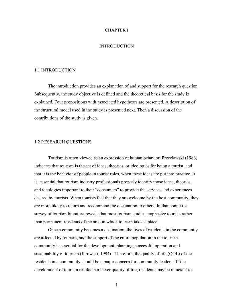
1.1 INTRODUCTION
The introduction provides an explanation of and support for the research question.
Subsequently, the study objective is defined and the theoretical basis for the study is
explained. Four propositions with associated hypotheses are presented. A description of
the structural model used in the study is presented next. Then a discussion of the
contributions of the study is given.
1.2 RESEARCH QUESTIONS
Tourism is often viewed as an expression of human behavior. Przeclawski (1986)
indicates that tourism is the set of ideas, theories, or ideologies for being a tourist, and
that it is the behavior of people in tourist roles, when these ideas are put into practice. It
is essential that tourism industry professionals properly identify those ideas, theories,
and ideologies important to their “consumers” to provide the services and experiences
desired by tourists. When tourists feel that they are welcome by the host community, they
are more likely to return and recommend the destination to others. In that context, a
survey of tourism literature reveals that most tourism studies emphasize tourists rather
than permanent residents of the area in which tourism takes a place.
Once a community becomes a destination, the lives of residents in the community
are affected by tourism, and the support of the entire population in the tourism
community is essential for the development, planning, successful operation and
sustainability of tourism (Jurowski, 1994). Therefore, the quality of life (QOL) of the
residents in a community should be a major concern for community leaders. If the
development of tourism results in a lesser quality of life, residents may be reluctant to
2
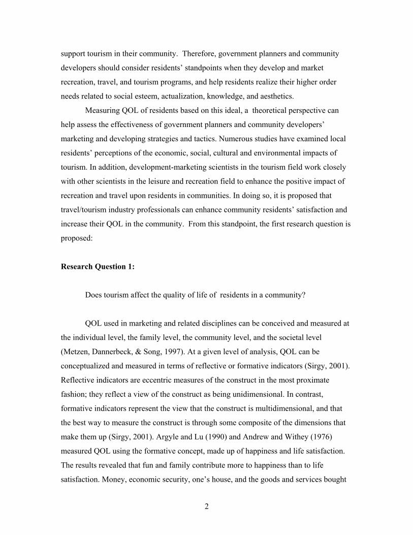
support tourism in their community. Therefore, government planners and community
developers should consider residents’ standpoints when they develop and market
recreation, travel, and tourism programs, and help residents realize their higher order
needs related to social esteem, actualization, knowledge, and aesthetics.
Measuring QOL of residents based on this ideal, a theoretical perspective can
help assess the effectiveness of government planners and community developers’
marketing and developing strategies and tactics. Numerous studies have examined local
residents’ perceptions of the economic, social, cultural and environmental impacts of
tourism. In addition, development-marketing scientists in the tourism field work closely
with other scientists in the leisure and recreation field to enhance the positive impact of
recreation and travel upon residents in communities. In doing so, it is proposed that
travel/tourism industry professionals can enhance community residents’ satisfaction and
increase their QOL in the community. From this standpoint, the first research question is
proposed:
Research Question 1:
Does tourism affect the quality of life of residents in a community?
QOL used in marketing and related disciplines can be conceived and measured at
the individual level, the family level, the community level, and the societal level
(Metzen, Dannerbeck, & Song, 1997). At a given level of analysis, QOL can be
conceptualized and measured in terms of reflective or formative indicators (Sirgy, 2001).
Reflective indicators are eccentric measures of the construct in the most proximate
fashion; they reflect a view of the construct as being unidimensional. In contrast,
formative indicators represent the view that the construct is multidimensional, and that
the best way to measure the construct is through some composite of the dimensions that
make them up (Sirgy, 2001). Argyle and Lu (1990) and Andrew and Withey (1976)
measured QOL using the formative concept, made up of happiness and life satisfaction.
The results revealed that fun and family contribute more to happiness than to life
satisfaction. Money, economic security, one’s house, and the goods and services bought
3
in the market contribute to life satisfaction more than to happiness. Similarly, Michalos
(1980) showed that evaluations of ten measured life domains (health, financial security,
family life, and self-esteem, etc.) were more closely related to life satisfaction (which
refers to the satisfaction that people may feel toward their overall living conditions and
life accomplishments) than to happiness.
Measuring QOL overall or within a specific life domain can be done through
subjective indicators or objective indicators (Samli 1995). Objective indicators are
indices derived from areas such as ecology, human rights, welfare, education, etc.
According to Diener and Suh (1997), the strength of objective indicators is that these
usually can be relatively easily defined and quantified without relying heavily on
individual perceptions. By including measures across various life domains, researchers
are able to capture important aspects of society that are not sufficiently reflected in purely
economic terms.
Perdue, Long and Gustke (1991) investigated how the level of tourism
development affected QOL of the residents in the community by using objective
measures such as population, economic level (income), education, health, welfare, and
crime rate in the community. They concluded that tourism affected net population
migration, the types of jobs, education expenditure, the overall level of education and
available health care; however, it did not affect population age distribution,
unemployment rates, welfare needs and costs, and the per capita number of crimes. In a
study of objective indicators of rural tourism impact, Crotts and Holland (1993)
concluded that tourism affects positively the quality of life of rural residents in terms of
income, health, recreation, personal services and per capita sales, and negatively the level
of poverty.
Subjective indicators are mostly based on psychological responses, such as life
satisfaction, job satisfaction, and personal happiness, among others. Despite the
impression that subjective indicators seem to have lesser scientific credibility, their major
advantage is that they capture experiences that are important to the individual (Andrew &
Withey, 1976). By measuring the experience of well-being on a common dimension such
as degree of satisfaction, subjective indicators can more easily be compared across
domains than can objective measures, which usually involve different units of
4
measurement. Many researchers have considered overall life satisfaction as the sum of
satisfactions in important life domains measured by subjective indicators.
The great majority of more recent definitions, models, and instruments have
attempted to break down the QOL construct into consequent domains. There is little
agreement, however, regarding either the number or scope of these domains. The possible
number of domains is large. When he asked respondents to indicate how various domains
of life are important to them, Abrams (1973) found the four domains were health,
intimacy, material well being, and productivity. Campbell, Converse, and Rodgers (1976)
asked people to rate domain importance on a five point scale; they found that four
domains were scored 91%, 89%, 73%, and 70% for health, intimacy, material well being,
and productivity, respectively. Flanagan (1978) and Krupinski(1980) found that the five
domains were regarded as very important aspects of their lives by a large majority of
people, and scored health, 97%; intimacy, 81%; emotional, 86%; material well being,
83%; and productivity, 78%. Cummins (1997) proposed two additional domains of safety
and community. Cummins, McCabe, Romeo, and Gullone (1994) have provided both
empirical and theoretical arguments for the use of seven domains, these being material,
health, productivity, intimacy, safety, community, and emotional well-being. Finally,
Cummins (1996) reviewed 32 studies and found 173 different terms that have been used
to describe domains of life satisfaction. He attempted to identify clear QOL domains and
found that a majority supported seven of the proposed domains, such as emotional well-
being, health, intimacy, safety, community, material well-being, and productive activity.
However, tourism is most likely to affect material well being, community well-being,
emotional well-being, and health and safety well-being domains, as this study proposes.
Perdue, Long and Kang (1999) studied how residents’ perception of community
safety, community involvement, local political influence, and changes in job
opportunities, social environment, and community congestion influenced their quality of
life in the community. Their findings showed that the key community characteristics
affecting residents’ QOL were community safety, social environment, and community
involvement. In that sense, the research question 2 and 3 are proposed.

5
Research Question 2:
Does tourism impact affect the particular life domain?
Research Question 3:
Does the particular life domain affect overall QOL of the residents in the
community?
Over the past decades, interest in tourism development as a regional economic
development strategy has grown dramatically (Getz, 1986; Gursoy, Jurowski, & Uysal,
2002; Jurowski, Uysal, & Williams, 1997; Liu & Var, 1986). Increasingly, tourism is
perceived as a potential basic industry, providing local employment opportunities, tax
revenues, and economic diversity. As a result, concerns over the potential impacts of
tourism development have created a significant demand for comprehensive planning and
a need for systematic research on the effects of tourism on local quality of life (Crotts &
Holland, 1993; Loukissas, 1983; Murphy, 1983; Pearce, 1996; Perdue, Long & Gustke,
1991; Perdue, Long & Kang, 1999). The objectives and goals of organizations in
communities may be very different, but one of the commonalities that they share may be
to improve the quality of life in their communities.
Butler (1980) explained why tourism almost always becomes unsustainable.
Using a life-cycle model, he described how initially, a small number of adventurous
tourists explore a natural attraction, leading to the involvement of local residents and
subsequent development of the area as a tourist destination. The number of tourists
thereafter grows, eventually consolidating and maturing into mass tourism. Unless the
tourism products are rejuvenated, the result is stagnation and eventual decline when
overuse beyond the destination’s carrying capacity has been reached and then exceeded,
making mass tourism unsustainable. Mass tourism can generate large quantities of waste,
a problem particularly compelling in developing countries, in which systems for sewage
treatment and solid waste disposal are not well developed. As mass tourism adversely
affects the environment, environmental degradation in turn adversely affects tourism
demand, leading to its probable decline. Ironically, once tourists snub the destination, the
6
best source of money to repair the tourists’ damage dries up as well. Consequently, these
results reach the perceived negative attitudes of locals and affect the quality of life of the
residents in the community in negative ways.
The impact of tourism at the upper level of development may be most detrimental
to residents’ life satisfaction. Allen, Long, Perdue, and Kieselbach (1988) examined
changes in resident perceptions according to tourism development stages. Their findings
generally support tourism development cycle theories. The perceptions of tourism’s
impacts increased with increasing levels of tourism development, and resident support for
additional tourism development initially increased with increasing levels of actual
development, but attitudes became less favorable when tourism reached its maximum
status.
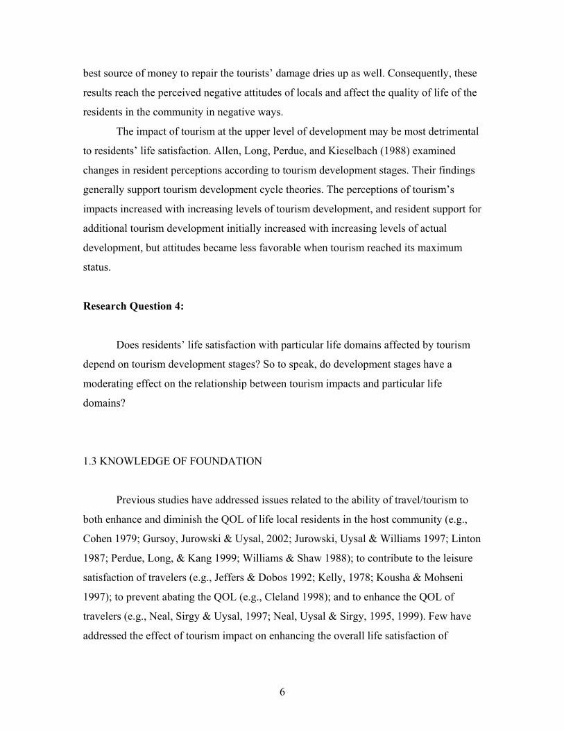
Research Question 4:
Does residents’ life satisfaction with particular life domains affected by tourism
depend on tourism development stages? So to speak, do development stages have a
moderating effect on the relationship between tourism impacts and particular life
domains?
1.3 KNOWLEDGE OF FOUNDATION
Previous studies have addressed issues related to the ability of travel/tourism to
both enhance and diminish the QOL of life local residents in the host community (e.g.,
Cohen 1979; Gursoy, Jurowski & Uysal, 2002; Jurowski, Uysal & Williams 1997; Linton
1987; Perdue, Long, & Kang 1999; Williams & Shaw 1988); to contribute to the leisure
satisfaction of travelers (e.g., Jeffers & Dobos 1992; Kelly, 1978; Kousha & Mohseni
1997); to prevent abating the QOL (e.g., Cleland 1998); and to enhance the QOL of
travelers (e.g., Neal, Sirgy & Uysal, 1997; Neal, Uysal & Sirgy, 1995, 1999). Few have
addressed the effect of tourism impact on enhancing the overall life satisfaction of

7
residents in a community. Enhancing the life satisfaction of individual residents is
believed to improve their QOL in a community.
Most travel and tourism textbooks address the issue of the impacts of tourism as
an important component which needs to be considered by decision makers involved with
the planning of tourism (Gee, Mackens, & Choy, 1989; Gunn, 1994; McIntosh, Goeldner,
& Ritchie, 1995; Murphy, 1983). De Kadt (1979) pointed out the general failure of
tourism destination planners to establish a clear framework to determine which questions
need to be considered, and what factors should enter into their decision-making.
Similarly, Mathieson and Wall (1982) present a synthesis of the research on the impacts
of tourism, and analyze tourism impact studies that have focused on interrelationships of
a combination of phenomena associated with tourism development.
The economic impact of tourism has been commonly viewed as a positive force
which increases total income for the local economy, foreign exchange earnings for the
host country, direct and indirect employment, and tax revenues; it also stimulates
secondary economic growth (Bryant & Morrison, 1980; Gursoy et al., 2002; Jurowski et
al., 1997; Peppelenbosh & Templeman, 1989; Uysal, Pomeroy, & Potts, 1992). Cultural
impact studies consider tourism as a cultural exploiter (Fanon, 1966; Greenwood, 1977;
Pears, 1996; Young, 1977). Additionally, tourism has frequently been criticized for the
disruption of traditional social structures and behavioral patterns (Butler, 1975; Kousis,
1989). However, tourism has also been viewed as a means of revitalizing cultures when
dying customs are rejuvenated for tourists (Witt, 1990).
Studies of the environmental impact of tourism focus on tourism development,
stress and preservation (Farrell & Runyan, 1991). Alpine areas, coastlines, islands, lakes,
and habitat areas are generally sensitive to the intense usage resulting from tourism
development (Murph, 1983). Krippendorf (1982) urges planners to protect the resources
on which tourism is dependent.
Most of our knowledge about residents’ attitudes toward tourism has come from
the analysis of surveys, which ask respondents to indicate a level of agreement with
positive or negative statements about the impact of tourism (Allen, Hafer, Long &
Perdue, 1993; Ap & Crompton, 1998). Some researchers found a linear relationship
between support for tourism and certain perceptions and personal characteristics (Perdue,
8
Long & Allen, 1987). Other studies have inferred that there are varying levels of support
for tourism within a community (Dogan, 1989; Doxey, 1975), as well as differences in
support for tourism the perceptions of local residents in the host community (e.g. Cohen,
1978; Linton 1987; Jurowski, Uysal, & Williams, 1997; Perdue, Long, & Kang, 1999;
Williams & Shaw 1988).
A few studies have addressed the effect that tourism has on enhancing the overall
life satisfaction of residents in a community. Enhancing the life satisfaction of individual
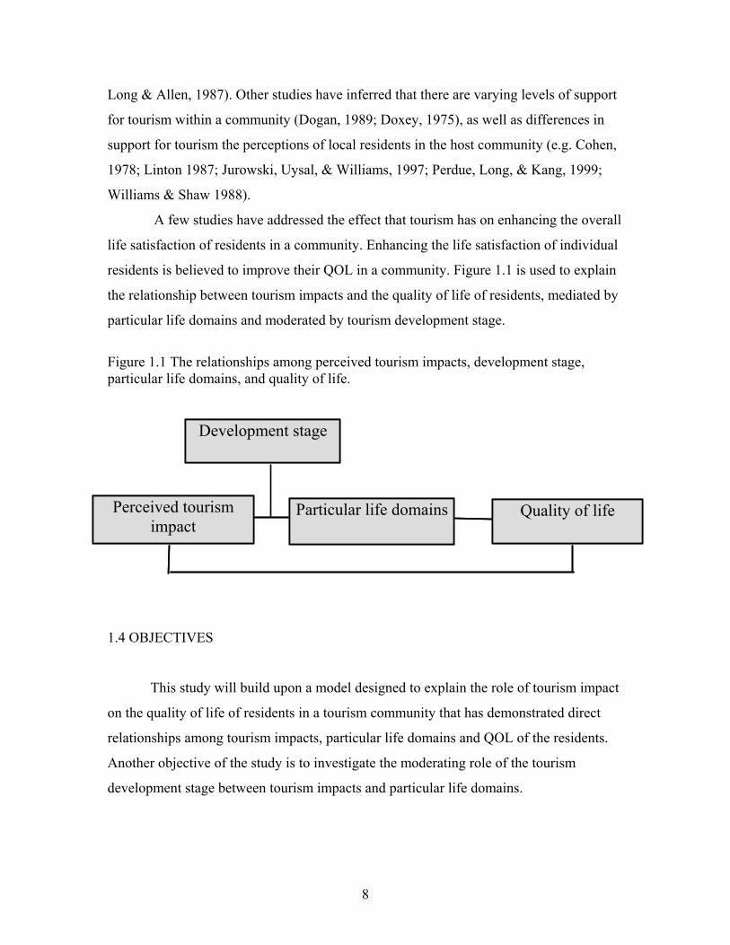
residents is believed to improve their QOL in a community. Figure 1.1 is used to explain
the relationship between tourism impacts and the quality of life of residents, mediated by
particular life domains and moderated by tourism development stage.
Figure 1.1 The relationships among perceived tourism impacts, development stage, particular life domains, and quality of life.
1.4 OBJECTIVES
This study will build upon a model designed to explain the role of tourism impact
on the quality of life of residents in a tourism community that has demonstrated direct
relationships among tourism impacts, particular life domains and QOL of the residents.
Another objective of the study is to investigate the moderating role of the tourism
development stage between tourism impacts and particular life domains.
Development stage
Quality of life Subjective well-being Perceived tourism impact
Development stage
Quality of life Particular life domains Perceived tourism impact
9
The research objectives are to identify:
1) The direct effects of the economic, social, cultural, and environmental
impacts of tourism on the quality of life of residents.
2) The direct effects of the perception of the economic, social, cultural,
and environmental impacts of tourism on particular life domains.
3) The direct effects of particular life domains on the quality of life of
residents.
4) The moderating effects of the tourism development stage between the
perception of economic, social, cultural and environmental impacts of
tourism and particular life domains.
1.5 THEORETICAL BASIS
To date, little is known about the effect of tourism impacts on the quality of life of
residents in communities. This study is generally predicated on the importance of social
impact assessment as a component of both tourism (Blank, 1989; Loukissas, 1983; Marsh
& Henshal, 1987) and comprehensive community planning (Freudenburg, 1997;
Gramling & Freudenburg, 1992; Inter-organizational Committee, 1994). A primary goal
of such planning is to enhance resident QOL (O’Brien & Ayidiya, 1991). It is important
to extend these descriptive studies of tourism impacts to begin developing and testing
alternative theoretical explanations of their effects on residents’ QOL.
A theoretical explanation of tourism impact on resident QOL exists in the
literature. Tourism literature includes several “tourism development cycle” theories
(Butler, 1980; Doxey, 1975; Lundberg, 1990; Smith, 1992), all of which are generally
based on the concept of social carrying capacity (Long, Perdue & Allen, 1990; Madrigal,
10
1993). The underlying premise of these theories is that residents’ QOL will improve
during the initial phases of tourism development, but reach a “carrying capacity” or
“level of acceptable change” beyond which additional development causes negative
change. These studies suggest that communities have a certain capacity to absorb tourists.
Growth beyond this capacity or threshold may result in negative social and
environmental impacts and diminishing returns on tourism investments. If carrying
capacity is determined, then economic, social and environmental benefits can be
optimized and negative consequences minimized (Allen, Long, Perdue, & Kieselbach,
1988).
Martin and Uysal (1990) investigated the relationship between carrying capacity
and tourism life cycle: management and policy implication. Martin and Uysal (1990)
defined carrying capacity as the number of visitors that an area can accommodate before
negative impact occurs, either to the physical environment, the psychological attitude of
tourists, or the social acceptance level of hosts. They also found that each development
stage has its own carrying capacity. Butler (1980) explained that tourist areas go through
a recognizable cycle of evolution; he used an S-shaped curve to illustrate different stages
of popularity.
O’Reilly (1986) describes two schools of thought concerning carrying capacity.
In one, carrying capacity is considered to be the capacity of the destination area to absorb
tourism before the host population feels negative impacts. The second school of thought
contends that tourism carrying capacity is the level beyond which tourist flows will
decline because certain capacities, as perceived by tourists themselves, have been
exceeded, causing destination areas to cease to satisfy and attract tourists. Mathieson and
Wall (1982) say that carrying capacity is the maximum number of people who can use a
site without an acceptable alteration in the physical environment and without an
acceptable decline in the quality of experience gained by visitors. O’Reilly (1986) claims
that carrying capacities can be established not only from a physical perspective but also
for the social, cultural, and economic subsystems of the destination.
Economic carrying capacity, as described by Mathieson and Wall (1982), is the
ability to absorb tourist functions without squeezing out desirable local activities. They
define social carrying capacity as the level at which the host population of an area

11
becomes intolerant of the presence of tourists. Economic carrying capacity involves two
dimensions: physical and psychological. Physical carrying capacity is the actual physical
limitations of the area-the point at which no more people can be accommodated. It also
includes any physical deterioration of the environment caused by tourism. Psychological
carrying capacity has been exceeded when tourists are no longer comfortable in the
destination area, for reasons that can include perceived negative attitudes of the locals,
crowding of the area, or deterioration in the physical environment.
Social capacity is reached when the local residents of an area no longer want
tourists because they are destroying the environment, damaging the local culture, or
crowding them out of local activities. According to Martin and Uysal (1990), the carrying
capacity for a destination area is different for each life cycle stage of the area. For
instance, in the beginning stage, the carrying capacity might be nearly infinite on a social
level, but, because of lack of facilities, few tourists can actually be accommodated. In this
instance, the physical parameters may be the limiting factor. At the other extreme is the
maturity stage, at which facility development has reached its peak and large numbers of
tourists can be accommodated, but the host community is showing antagonism toward the
tourist. The changes in the attitudes of locals toward tourists have been documented by
Doxey (1975) as an index of irritation, which shows feelings that range from euphoria to
regret that tourism came to the area. At this point, social parameters become the limiting
factor. Understanding the life cycle concept and its interrelationship with the concept of
carrying capacity is important to those concerned with establishing a tourism policy for a
destination area. Only through life cycle position determination and utilization of an
optimal carrying capacity can the future of a destination area be controlled.
At some point, the negative effects of too many tourists cause permanent residents
to resent tourists altogether. Doxey (1975) predicted residents’ change in perceptions and
attitudes in responses toward visitors by indexing the progression of feeling from
euphoria, enthusiasm, and hope to apathy and irritation. Negative feelings result from
tourists’ encroachment, and eventually evolve into overt antagonism when the
environment and community life have been damaged beyond repair. As has happened,
the transformation from residents’ welcoming visitors to despising them can be speeded
12
along when tourists introduce disease agents or other medical issues that otherwise could
have been avoided.
Other researchers have tried to explain why residents respond to the impact of
tourism the way they do and why there are various levels of support within the same
community (Gursoy, Jurowski & Uysal, 2002; Jurowski, Uysal & Williams, 1997).
Social exchange theory has provided an appropriate framework for Gursoy et al.’s study
questions about resident reactions to tourism.
Social exchange theorist, Emerson (1972) has adopted principles from behavioral
psychology theory and utilitarian economic theory to formulate the principles of social
exchange. Psychological behavioral principles are principles of reward and punishment,
which have been brought into modern social exchange as rewards and costs (Turner,
1986). The theory assumes that individuals select exchanges after having assessed
rewards and costs.
On the other hand, according to Emerson (1972), utilitarian principles propose
that humans rationally weigh costs against benefits to maximize material benefits.
Exchange theorists have reformulated utilitarian principles by recognizing that humans
are not economically rational, and do not always seek to maximize benefits, but instead
engage in exchanges from which they can reap some benefit without incurring
unacceptable costs (Turner, 1986). Homans (1967) proposed that humans pursue more
than material goals in exchange, and that sentiments, services, and symbols are also
exchange commodities. Thus, the exchange process includes not only tangible goods
such as money and information, but also non-materialistic benefits such as approval,
esteem, compliance, love, joy, and affection (Turner, 1986). The perception of the impact
of tourism for this study is a result of this assessment. The way that people perceive the
impact of tourism affects their subjective well-being domains, and will affect their life
satisfaction. However, individuals who evaluate the exchange as beneficial will perceive
the same impact differently than someone who evaluates the exchange as harmful.
A few researchers have attempted to apply the principles of social exchange in an
effort to explain the reaction of residents. For example, Perdue, Long and Allen (1987)
used the logic in social exchange theory to explain the differences in tourists’ perceptions
and attitudes based on variance in participation in outdoor recreation. They hypothesized

13
that outdoor recreation participants, when compared to non-participants, would perceive
more negative impacts from tourism because of the opportunity costs associated with
tourists’ use of local outdoor recreation areas. However, their findings failed to support
this hypothesis. They explained that the reason for this failure was that residents might
feel that tourism had improved rather than reduced the quality of outdoor recreation
opportunities. Support for this supposition can be found in the results of several studies,
which found that residents view tourism as a benefit to increase recreational opportunities
(Keogh, 1989; Liu, Sheldon & Var, 1987).
Ap (1992) also based his research on social exchange principles in an exploration
of the relationship between residents’ perceptions of their power to control tourism and
their support for tourism development. However, his finding revealed that the power
discrepancy variable did not emerge as the most important variable in explaining the
variance of perceived tourism impacts. He suggested that a study of the value of
resources and perceived benefits and costs might provide further insight into exchange
relationships, and that a quasi-experimental design might better test power discrepancy as
a factor influencing host community residents’ attitudes toward tourism.
Another study (Jurowski, Uysal & Williams, 1997) explored how the interplay of
exchange factors influences not only the attitude about tourism but also the host
community residents’ perceptions of tourism’s impacts. This model explained how
residents weighed and balanced seven factors that influenced their support for tourism.
The study demonstrated that potential for economic gain, use of tourism resources,
ecocentric (support for eco-tourism) attitude, and attachment to the community affect
residents’ perceptions of the impacts and modify, both directly and indirectly, residents’
support for tourism.
The model in Figure 1.2 describes that tourism is: a system of exchange between
tourists and the businesses/services at the destination; an exchange between
businesses/services and the residents in the host community; and an exchange between
tourists and residents in the host community. Theoretically, if any component perceived
the distribution as positive, it would seek to maintain the exchange relationship. On the
other hand, if that component perceives a negative distribution, it will seek to discontinue
the relationship. However, the profit from tourism depends on the carrying capacity of

14
the community. As the carrying capacity permits, residents may tolerate the costs of
tourism. However, once the carrying capacity reaches its maximum capacity, the
residents will not tolerate the costs any more.
Figure 1.2 Tourism Exchange System modified from Jurowski, 1994
Based on the previously-described theoretical framework, the current study
proposes the effect of tourism impacts on the quality of life of residents in a community
using economic, social, cultural, and environmental impact assessments as components of
tourism. Also, the study suggests that the benefits of perceived tourism impacts enhance
the QOL of the residents affected by particular life domain indicators, as mediator
Tourists at the destination
Profit and non-profit
organization or business
Residents in the community
15
variables. The specific hypothesized relationships between the aspects of tourism impacts
and overall life satisfaction are explained in the next section.
1.6. PROPOSITIONS
Social capacity is reached when the local residents of an area no longer want
tourists because they are destroying the environment, damaging the local culture, or
crowding them out of local activities. At some point, the negative effects of too many
tourists cause permanent residents to resent tourists altogether. Doxey (1975) predicts
residents’ changes in perceptions and attitudes in responses toward visitors by indexing
the progression of feeling from euphoria, enthusiasm, and hope to apathy and irritation.
Negative feelings result from tourists’ encroachment, and eventually evolve into overt
antagonism when the environment and community life have been damaged beyond
repair. Figure 1.3 shows the direct relationships between the residents’ perceptions of
tourism impact and their life satisfaction.
Proposition 1: Residents’ perceptions of tourism impacts affect their QOL in the
community.
Hypothesis 1: Residents’ life satisfaction in general is a positive function of their
perceptions of the benefits of the economic impact of tourism.
Hypothesis 2: Residents’ life satisfaction in general is a positive function of their
perceptions of the benefits of the social impact of tourism.
Hypothesis 3: Residents’ life satisfaction in general is a positive function of their
perceptions of the benefits of the cultural impact of tourism.
16
Hypothesis 4: Residents’ life satisfaction in general is a positive function of their
perceptions of the benefits of the environmental impact of tourism.
After the carrying capacity at the destination is reached, residents’ unpleasant
perception of the tourism impacts takes place in the physical environment. This feeling
gradually becomes more and more negative; affects residents’ social consciousness (their
general feeling of community well-being and health and safety well-being); and
influences their possessions, material well-being, and emotional well-being in the
community. Residents’ social consciousness and satisfaction of material possessions
finally affect life satisfaction in general.
Proposition 2: Residents’ satisfaction in a particular life domain is affected by the
perception of the particular tourism impact dimension.
Hypothesis 5: The material well-being domain is a positive function of the perception of
the economic impact of tourism.
Hypothesis 6: The community well-being domain is a positive function of the perception
of social impact of tourism.
Hypothesis 7: The emotional well-being domain is a positive function of the perception
of the cultural impact of tourism.
Hypothesis 8: The health and safety well-being domain is a positive function of the
perception of environmental impact of tourism.
Proposition 3: Residents’ satisfaction in particular life domains affects residents’ life
satisfaction in general.

17
Hypothesis 9: Residents’ life satisfaction in general is a positive function of the material
well-being domain.
Hypothesis 10: Residents’ life satisfaction in general is a positive function of the
community well-being domain.
Hypothesis 11: Residents’ life satisfaction in general is a positive function of the
emotional well-being domain.
Hypothesis 12: Residents’ life satisfaction in general is a positive function of the health
and safety well-being domain.
The perception of various social, economic, cultural, and environmental impacts
is related strongly to the level of tourism development. This relationship suggests that the
impact of tourism at the upper level of development may be most detrimental to
residents’ life satisfaction. Allen et al. (1988) examined changes in resident perceptions
of seven dimensions of community life across 20 communities classified on the basis of
the percentage of retail sales derived from tourism. Their finding generally supports
tourism development cycle theories. According to Allen et al. (1988, p.20), “Lower to
moderate levels of tourism development were quite beneficial to the study communities,
but as development continued, residents’ perceptions of community life declined,
particularly as related to public services and opportunities for citizens’ social and
political involvement.” Using the same data set, Long, Purdue, and Allen (1990)
concluded that (1) perceptions of tourism’s impacts increased with increasing levels of
tourism development and (2), residents’ support for additional tourism development
initially increased with increasing levels of actual development, but reached a threshold
social carrying capacity level beyond which attitudes became less favorable.
Proposition 4: The relationship between residents’ perception of tourism impacts and
their satisfaction in particular domains is moderated by the tourism development cycle.
18
Hypothesis 13: The relationship between the economic impact of tourism and material
well-being is strongest in relation to the beginning and growth stages of the tourism
development cycle and weakest in relation to the maturity and decline stages.
Hypothesis 14: The relationship between the social impact of tourism and community
well-being is strongest in relation to the maturity and decline stages of the tourism
development cycle and weakest in relation to the beginning and growth stages.
Hypothesis 15: The relationship between the cultural impact of tourism and emotional
well-being is strongest in relation to the maturity and decline stages of the tourism
development cycle and weakest in relation to the beginning and growth stages.
Hypothesis 16: The relationship between the environmental impact of tourism and health
and safety well-being is strongest in relation to the maturity and decline stages of the
tourism development cycle and weakest in relation to the beginning and growth stages.
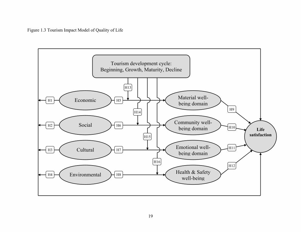
The specific hypothesized relationships are shown in Figure 1.3. The tourism
impacts upon QOL model depicted in Figure 1.3 is used to explain the relationship
between the tourism impacts and life satisfaction in general mediated by particular life
domains and moderated by tourism development stage. This model depicts that overall
life satisfaction is derived from the satisfaction of particular life domains such as material
well-being, community well-being, emotional well-being, and health and safety well-
being. A specific tourism impact dimension affects satisfaction with each life domain.
For instance, perceived tourism economic impact will strongly affect the satisfaction with
material well-being domain, but will not affect the community well being domain,
emotional well-being domain, and health and safety well-being domains. Also, residents’
perception of tourism impacts on particular life domains will vary according to different
tourism development stages.
19
Figure 1.3 Tourism Impact Model of Quality of Life
Emotional well-being domain
Economic Material well-being domain
Social
Cultural
Environmental
Community well-being domain
Tourism development cycle: Beginning, Growth, Maturity, Decline
Health & Safety well-being
H5
H6
H7
H8
H9
H10
H11
H12
H13
H1
H2
H3
H4
Life satisfaction
H14
H15
H16
20
1.7. STRUCTURAL MODEL OF THE STUDY
Using a structural equation model allows a theoretical scheme to be developed
and tested which is based on a sequence of events. The model in Figure 1.3 shows the
hypothesized relationships. The model describes the logical flow of factors related to
residents’ perception of tourism, which affects residents’ life satisfaction.
The model structurally depicts that satisfaction with life in general is derived from
satisfaction with particular life domains. For example, overall life satisfaction is derived
from the material well-being domain, which includes consumer well-being related to
material possessions. The model illustrates that overall life satisfaction is also derived
from satisfaction with the social well-being dimension. The community well-being
dimension consists of the relation between community environment and satisfaction with
community service. The model also proposes that overall life satisfaction is derived from
satisfaction with emotional well-being, which is related to the spiritual well-being and
leisure well-being dimension. According to Neal, Sirgy, and Uysal (1997), the leisure
well-being dimension is obtained from the components of leisure experiences at home
and satisfaction with a travel/tourism trip experience. The travel/tourism trip experience
is most likely derived from leisure satisfaction with travel/tourism services and leisure
satisfaction stemming from leisure trip reflections.
Figure 1.3 illustrates that overall life satisfaction is derived from residents’
perception of various tourism impacts such as economic, social, cultural, and
environmental impacts. However, various tourism impact dimensions also affect
particular life domains to formulate the general life satisfaction. Finally, the relationships
between tourism impact dimensions and particular life domains are moderated by the
tourism development stage.
In this model, tourism impacts are considered to be the exogenous variables (i.e.,
those that are not predicted by any other variables in the model); the particular life
domains and QOL of residents are endogenous variables (i.e., variables that are
dependent variables in at least some of the relationships in the model). Reflective
satisfaction of life is the ultimate dependent variable (the one that is affected by all of the
others). Satisfaction with particular life domains (material well-being, community well-
21
being, emotional well-being and health and safety well-being) is considered to be the
mediating variable (which either directly or indirectly affects the ultimate dependent
variable) between perception of tourism impact and the life satisfaction variable. All
relationships between the perception of tourism impact and the particular life satisfaction
variable depend on tourism development stages in a destination.
1.8 CONTRIBUTION OF THE STUDY
The potential contribution of this study can be seen from both theoretical and
practical perspectives:
1.8.1. Theoretical advancement in tourism study
This study contributes to a theoretical advancement in the field of tourism by
proposing a model to explain the effects of the interaction of elements important to
individuals and their perceptions of the impact of tourism on their life satisfaction. It adds
to existing knowledge by creating a model that explains factors regarding how
individuals’ perceptions of tourism impacts vary according to the destination
development stage, the factors which influence the particular life domains, and the
factors which subsequently affect individuals’ life satisfaction. The study’s uniqueness
lies in the interactive treatment of the variables. The dynamic nature of the proposed
structural model provides new insights into understanding factors which affect the quality
of life of residents in the community.
1.8.2. Practical application for the tourism-planning program
The findings of this study will aid in the planning of strategic development
programs for tourist destinations. The model can be helpful in understanding factors that
influence the quality of life of residents in the tourism community. An understanding of
what is important to the individuals within a community will assist resource planners to

22
preserve that which is most valued. Furthermore, communication messages designed to
elicit support for tourism development can be more effectively designed if planners are
cognizant of the values of their audience.
1.9 CHAPTER SUMMARY
Chapter I presented the overview of the study and included the statement of the
problem, theoretical background of the problem, the research question, the theoretical
framework of the study, and the theoretical model that is based of the study. In Chapter
II, a review of the relevant literature is presented.
23
CHAPTER TWO
LITERATURE REVIEW
2.1 INTRODUCTION
The aim of this literature review is to generate awareness, understanding, and
interest for studies that have explored a given topic in the past. This chapter defines the
current level of knowledge about the theoretical and conceptual research on tourism
impact and quality of life studies derived from different sources, such as sociology,
planning, and marketing. First, this chapter explains the relevance of this research. In the
second section, the concept of carrying capacity, tourism life cycle with explanation of
the characteristics of different stages, and their interrelationships with tourism impacts
and residents’ QOL are reviewed. The third section addresses the review of tourism
impacts and its dimensions. The last section presents the particular life domains related to
tourism.
2.2 RELEVANCE OF THE RESEARCH
Tourism is an interdisciplinary field and involves a number of different industries
and natural settings. Planning is essential to stimulate tourism development and its
sustainability. Without tourism planning, many unintended consequences may develop,
causing tourist and resident dissatisfaction. These include damage to the natural
environment, adverse impacts upon the cultural environment, and a decrease in potential
economic benefits. The negative experience of many unplanned tourist destinations and
the success of local and regional planned destinations demonstrate that tourism
development should be based on a planning process that includes a solid assessment of
the resources at the destination and their attractiveness potential (Blank, 1989; Formica,
2000; Gunn, 1994; Inskeep, 1994).
24
Some government and private researchers have studied the measurement of
tourism resources and the development of appropriate tourism plans. Resource
assessment and planning become increasingly important in order to achieve long-term
development of new or developing tourism destinations. Planning is also important for
developed tourist destinations at which major efforts are generally focused on revitalizing
the area and sustaining its attractiveness over time (Dragicevic, 1991; Formica, 2000;
McIntosh, Goeldner, & Ritchie, 1995; Witt, 1991).
Other researchers have studied tourism impacts in planning marketable tourism
destinations within a community, and have demonstrated that tourism development has
costs as well as benefits. Tourists have been accused of destroying the very things that
they came to enjoy (Krippendorf, 1982). Early development planning focused on
economic benefits, with almost complete disregard for social and environmental impacts.
The planning and marketing of tourism have been primarily oriented towards the needs of
the tourist, but this planning should include efforts to manage the welfare of the host
population. Failure to consider the needs of the indigenous population has resulted in the
disruption or destruction of cultures and values, the disruption of economic systems, and
the deterioration of the physical and social environment. Tourism planning cannot
succeed by focusing only on resource assessment. Planning should employ holistic
approaches, including the QOL of residents in the community impacted by tourism.
Among the different theoretical explanations of tourism impact on residents’
QOL, the tourism literature includes several “tourism development cycle” theories
(Butler, 1980; Doxey, 1975; Smith, 1992), all of which are generally based on the
concept of social carrying capacity (Long, Perdue, Allen, 1990; Madrigal, 1993). The
underlying premise of these theories is that resident QOL will improve during the initial
phases of tourism development, but reach a “carrying capacity” or “level of acceptable
change” beyond which additional development may cause negative change. Butler (1980)
explained why tourism almost always becomes unsustainable. Using a life-cycle model,
he describes how initially, a small number of adventurous tourists explore a natural
attraction, leading to the involvement of local residents and subsequent development of
the area as a tourist destination. The number of tourists thereafter grows, eventually
consolidating and maturing into mass tourism. Unless tourism products are rejuvenated,
25
the result is stagnation and eventual decline when saturation beyond the destination’s
carrying capacity has been reached and then exceeded, making mass tourism
unsustainable.
These studies suggest that communities have a certain capacity to absorb tourists.
Growth beyond this capacity or threshold may result in negative social and
environmental impacts and diminishing returns on tourism investments. If carrying
capacity is determined, then economic, social and environmental benefits can be
optimized and negative consequences minimized (Allen, Long, Perdue, & Kieselbach,
1988). Consequently, sustainable development has become an important topic in tourism
literature. Because the host population is a key element in the success of a tourist
destination, sustainable tourism is dependent upon the willingness of the host community
to service tourists. From that standpoint, the next section explains tourism impact and its
related theories: carrying capacity and the tourism development cycle.
2.3 TOURISM IMPACTS
Impact studies emerged in the 1960s with much emphasis on economic growth as
a form of national development, measured in terms of "Gross National Product (GNP),”
rate of employment, and the multiplier effect (Krannich, Berry & Greider, 1989). The
1970s saw the impacts of tourism ventures on social-cultural issues (Bryden, 1973).
Environmental impacts of tourism became the sole concern of tourism researchers in the
1980s (Butler, 1980). 1990s tourism impact studies are an integration of the effects of the
previous determined impacts, leading to a shift from "Mass Tourism" to "Sustainable
Tourism" in the form of Eco-tourism, heritage tourism, and Community tourism
(Jurowski, Uysal, & Williams, 1997).
Tourism is an industry with enormous economic impacts. It is also an industry
that has many environmental and social consequences. A thorough understanding of each
component of the tourism phenomenon is essential so that those involved with planning,
management, and policy determination have a basis for decision-making.

26
The early research in this area focused on identifying the various perceived
impacts of tourism development (Belisle & Hoy, 1980; Liu, Sheldon, & Var, 1987; Liu &
Var, 1986; Perdue, Long, & Allen, 1987; Ross, 1992; Sheldon & Var, 1984). The major
impacts and variables have been identified, methodological approaches developed, and
problems and research needs delineated. Generally, residents recognized the positive
economic impact of tourism development, but were concerned with potentially negative
social and environmental impacts such as traffic congestion, crime, public safety issues,
and pollution.
This early research also typically examined differences in perceived impacts
among different types of local residents identified on the basis of socio-demographic
characteristics (Belisle & Hoy, 1980; Liu & Var, 1986; Milman & Pizam, 1988; Pizam,
1978); place of residence or distance from the tourism area of the community (Belisle &
Holy, 1980; Sheldon & Var, 1984); and economic dependency on tourism, measured both
as type of employment (Milman & Pizam, 1988; Pizam, 1978) and by comparing local
entrepreneurs, public official and other residents (Thomason, Crompton & Kamp, 1979;
Lankford, 1994; Murphy, 1983). This research found little consistent difference in
perceived tourism impacts by socio-demographic characteristics. Perceived impacts of
tourism decrease as distance between individuals’ homes and the tourism sector of the
community increases. Overall favorability of tourism impact perceptions increases with
the individual’s economic dependency on tourism.
Among tourism impact studies, the development of a tourism impact assessment
scale has also been one of the important topics espoused by scholars starting about two
decades ago (Chen, 2000). Pizam (1978) brought up tourism impact attributes; research
started using various resident attitude-related attributes to postulate-perceived tourism
impacts. Several researchers (Liu & Var, 1986; Liu, Sheldon & Var, 1987) further
distilled these attributes into fewer identical impact domains. After that, Lankford and
Howard (1994) found two factors from a 27-item tourism impact scale. McCool and
Martin (1994), who investigated mountain residents’ attitudes toward tourism, revealed
four factors including impacts, benefits, equity, and extent. However, Burns (1996), who
surveyed 102 inhabitants from 14 villages in the Solomon Islands, noticed that

27
respondents’ greatest concern was tourism’s socio-cultural impact with regard to the
demonstration effect and different cultural values of tourists.
According to the Inter-organization committee (1994), in general, there is
consensus on the types of impacts that need to be considered (social, cultural,
demographic, economic, social psychological). Also, political impacts are often included.
Recently Ap and Crompton (1998), in their effort to develop a reliable and valid impact
assessment scale, revealed a 35-item tourism impact scale that helps monitor sustainable
tourism development. However, the Inter-organization committee (1994) concluded that
the Social Impact Assessment (SIA) practitioner should focus on the more significant
impacts, use appropriate measures and information, provide quantification where feasible
and appropriate, and present the social impacts in a manner that can be understood by
decision makers and community leaders. In addition to investigations of scale
development, scholars have facilitated discussions on the issues of perceived economic,
social, cultural, and environmental impacts as a result of the presence of tourism. In the
next section, the major positive and negative impacts of tourism development is
discussed and summarized in Table 2.1.
2.3.1. Economic impacts
Tourism can create jobs, provide foreign exchange, produce return on investment
for emerging economics, bring technology, and improve living standards. The most
prominent benefits used to promote tourism development are the economic benefits that
communities can expect to derive from an increase in tourism activity. Every study of
resident perception of tourism impacts has included questions concerning economic
factors. The studies demonstrate that residents feel tourism helps the economy (Ritchie,
1988), that tourism increases the standard of living of host residents (e.g., Var & Kim,
1990), and that tourism helps the host community and country earn foreign exchange
(e.g., Ahmed & Krohn, 1992; Var & Kim, 1990). Also, tourism helps generate
employment (e.g., Ahmed & Krohn, 1992; Backman & Backman, 1997; Milman &
Pizam, 1987; Var & Kim, 1990), and increase revenue to local business (Backman &
Backman, 1997; Sethna & Richmond, 1978) and shopping facilities (Backman &
Backman, 1997). Services of all kinds are established and offered to tourists, which in
28
turn also serve local residents, and tourism generates the impetus to improve and further
develop community infrastructure and community service (Var & Kim, 1990). However,
tourism contributes to resentment concerning the employment of non-locals in
managerial and professional positions (e.g., Var & Kim, 1990). Tourism is related to
foreign domination of tourist services and facilities, increases in the cost of land and
housing, increases in prices of goods and services, increases in food and land prices, and
shortage of certain commodities (Var & Kim, 1990). Some researchers conclude that
residents agreed that tourism’s economic gains were greater than social costs (Liu & Var,
1986; Sheldon & Var, 1984; Weaver & Lawton, 2001). The vast majority of studies have
focused on employment opportunities, standard of living, the revenue that a community
derives from tourism activities, and cost of living.
Employment opportunities
A study conducted in British Columbia and Alberta Canada revealed that 87% of
the respondents felt that tourism was important to the number of jobs in the province,
while only 10% did not consider tourism an important contributor to employment
(Ritchie, 1988). In British Columbia, Belisle and Hoy (1980) found similar results in a
study which demonstrated that more than 84% of the respondents felt that tourism had
generated employment in the area. Tyrrell and Sheldon (1984) found that the creation of
jobs was one of the four most-frequently-mentioned benefits of tourism. Tosun (2002), in
his comparative study, also noted that the residents from Urgup, Turkey; Nadi, Fiji; and
Central Florida perceived employment opportunities as the positive tourism impact.
Many other studies found recognition by the residents of an increase in the number of
jobs from tourism (Davis, Allen, & Cosenza, 1988; Keogh, 1990; Liu & Var, 1986;
Pizam, 1978; Soutar & McLead, 1993; Weaver & Lawton, 2001; Tosun, 2002).
However, they also found that rapid construction led to heavy unemployment after
completion, and that the frequently seasonal nature of the industry disrupts the
employment structure.
29
Revenues from tourists for local business and standard of living
Like many other industries, the measure of receipts, and especially the net income
generated by those receipts, that a community can expect from tourism expenditure is
dependent upon government policies and a variety of local economic characteristics. One
study revealed that net income from tourism ranges from 25% to 90% of the total
receipts, depending upon the share of national and local interest in the tourist business
(Peppelenbosch & Templeman, 1989). Researchers have also asked residents if they felt
that tourism improved the economy (Allen et al., 1988; Bradley et al., 1989; Ritchie,
1988), provided an improved standard of living (Belisle & Holy, 1980; Tosun, 2002; Um
& Crompton, 1990), increased investment (Liu et al., 1987) and more business activity
(Prentice, 1993). The findings of these studies suggest that residents perceive an
improvement in income, standard of living, investments and business activities ensuing
from tourism activities. For example, Liu and Var (1986) reported that 90 % of the
residents in Hawaii agreed that tourism brought the community more investment and
local business.
However, the research on residents’ perception of tax revenues has been mixed.
In Rhode Island and Florida, residents expressed the belief that tax revenues derived from
tourist expenditures and tariffs could lower their own taxes (Tosun, 2002; Tyrrell &
Spaulding, 1984). Other researchers found that residents felt that their property taxes
increased as a result of tourism (Allen et al., 1993; Perdue et al., 1987). The majority of
residents in a British Columbian, Canada study did not agree that higher taxes should be
based on tourist expenditures (Belisle & Hoy, 1980). Residents did not much care about
the tax revenue for the local community, and perceived the tax as a negative impact of
tourism. Residents were unlikely to support tax expenditures for tourism if they did not
directly benefit from the industry (Prentice, 1993).
Cost of living
Negative economic impacts caused by an increase in the price of goods and
services have been perceived by residents in several surveys (Belisle & Hoy, 1980;
Keogh, 1989; Pizam, 1978; Tosun, 2002; Weaver & Lawton, 2001). Sheldon and Var
(1986) found only moderate agreement with a statement which suggested that increases
30
in tourism were the cause of increased prices of goods and services. Very few
respondents perceived tourism as the cause of the high cost of living in Zambia
(Husbands, 1989). Only 26% of a sample of New Brunswick, Canada residents felt that
the addition of a new park would cause price inflation in stores (Keogh, 1989).
Tourism can cause the price of land to rise rapidly, as noted by Lundburg (1990),
who found that the cost of land for new hotel construction rose from 1 percent to nearly
20 percent as the site was being developed. An early study by Pizam (1978) found that
residents viewed the cost of land and housing as a negative effect of tourism. More than
70% of the respondents in a Turkish study agreed that tourism increases property value
and housing prices (Tosun, 2002; Weaver & Lawton, 2001; Var, Kendall, & Tarakcoglu,
1985). However, other studies found more neutral attitudes. For example, Belisle and
Hoy (1980) determined that approximately 90% of respondents described the effect of
tourism on the cost of land and housing as neutral. About half of the respondents agreed
with the statement that tourism unfairly increases real estate costs, while, in a study of
Colorado residents, the other half disagreed (Perdue et al., 1987). These mixed findings
suggest that, even though dramatic real estate change has commonly been associated with
tourism development, the perception of the effect of these changes on residents is mixed
and irregular.
2.3.2. Social impacts
Tourism increases traffic congestion and crowdedness in the public area, and
brings social problems. Tourism also contributes to social ills such as begging, gambling,
drug trafficking, and prostitution, as well as the uprooting of traditional society, and
causes deterioratin of the traditional culture and customs of host countries (Ahmed &
Krohn, 1992, Var & Kim, 1990). Tourism contributes to an undesirable increase in the
consumption of alcohol, increased traffic congestion, and overcrowding because of
visitors (Backman & Backman, 1997). However, tourism brings more opportunities to
upgrade facilities such as outdoor recreation facilities, parks, and roads, but brings
crowdedness in theaters, movies, concerts, and athletic events (Lankford & Howard,
1994; Liu & Var, 1986).
31
Congestion
Another common theme in tourism resident attitude is that of crowding and
congestion, especially focused on traffic inconveniences. Rothman (1978) concluded
from his study on seasonal visitors that residents curtailed their activities during the peak
tourism season because of congestion. Liu and Var (1986) reported that residents in
Hawaii experienced crowdedness during the peak tourism seasons. Tyrrell and Spaulding
(1980) determined that the residents of the state of Rhode Island saw congested roads as
well as parking and shopping areas as a problem caused by tourism. Several other studies
also found that residents perceived that traffic was a major problem created by tourism
activities (Long et al, 1990; Keogh, 1990; Prentice, 1993). However, residents’
perceptions of the congestion caused by a major world event were less than predicted
(Soutar & McLeod, 1993). The majority of respondents in a Florida study did not agree
with a statement which suggested that traffic problems would disappear with the absence
of tourists (Davis et al., 1988). A concept that is closely related to congestion is that of
carrying capacity, which is defined in the literature as the level at which tolerance is
exceeded. The concept of carrying capacity is fully examined in section 2.3.5. The
residents in British Columbia, Canada, disagreed with statements that suggested that the
government should determine and enforce the carrying capacity of the island (Belisle &
Hoy, 1980).
Local service
Along with tax revenue and employment opportunities, residents have differing
views on the effects of tourism on local services. An early study by Sethna and
Richmond (1978) found that residents in the Virgin Islands agreed that the money
acquired from tourism contributed to the improvement of public services. Likewise,
residents in Cape Cod perceived a positive effect of tourism on local services (Pizam,
1978). The Rhode Island study found that only government officials perceived an
increase in the cost of police services (Tyrrell & Spaulding, 1980). An important finding
in the aspect of services was made by Murphy (1983), who examined the differing views
of residents, administrators, and business owners. He found that three groups differed in
their perception of the impact of tourism on local services. Allen et al. (1993) discovered
32
that tourism development increases sensitivity to change of public services, but
concluded that satisfaction with, and the availability of, services was more a function of
population size than tourism impact. One study found a relationship between satisfaction
with local services and tourism development. As development increased, satisfaction
with public services decreased. However, research results on the whole suggest that
residents feel that tourism improves local services (Keogh, 1989).
O’Leary (1976) found that residents view themselves as being forced out of
traditional leisure places through management agency regulations and indifference, and
through sharp increases in tourist visitations. In a similar vein, another qualitative study
uncovered resident expectations about losing leisure time because of the need to keep
longer business hours as tourism increased (Cheng, 1980). However, the results of most
quantitative studies imply that residents view tourism as a benefit, which increases
recreational opportunities (Perdue et al, 1991).
Increasing social problem
Crime is conceptualized here as any anti-social behavior including increased sale
or consumption of drugs and alcohol, as well as behavior considered immoral by the
society as a whole. Smith’s study (1992) of Pattaya, Thailand supported the view that
tourism development brought prostitution, drug abuse linked to many tourist deaths, sex-
related disease and injuries, and police corruption . A Florida study revealed that
residents perceived tourism as a causal factor in increasing crime and alcoholism (King,
Pizam, & Milman, 1993). On the other hand, Liu and Var (1986) reported that when they
asked residents in Hawaii if they perceived that tourism increased crime generally, only
37% of respondents felt that tourism contributed to crime. Other researchers who have
examined resident attitudes towards crime and tourism development also found little
perceived relationship between crime and tourism overall (Allen et al., 1993).
2.3.3. Cultural impacts
Even though tourism contributes to the renaissance of traditional arts and craft
(Var & Kim, 1990), tourism has frequently been criticized for the disruption of
traditional social and culture structures and behavioral patterns. Destination areas that

33
have embraced tourism for its economic benefits have witnessed heightened levels of
crime and prostitution, and displacement due to rising land costs and loss of the cultural
heritage of local people, particularly youth. Tourism has been charged not only with the
debasement of socio-cultural factors but also with degradation of the environment.
Acculturation takes place when two or more cultures come into contact for a sustained
period and ideas are exchanged (Liu & Var, 1986). In the case of relatively undeveloped
countries, however, local cultures and customs tend to be overwhelmed by more-
developed cultures, especially Western ones (Liu & Var, 1986; Weaver & Lawton,
2001). Moreover, some attraction operators will actually modify local standards to suit
tourists’ expectations. An example of acculturation is the accommodation of heritage:
residents try to convince tourists that corrupted and shortened cultural presentations are,
indeed, authentic. For example, the authentic Balinese dance has been shortened for
tourist events, and the dancers’ costumes have been made more colorful and attractive
than tradition dictates. Thus, tourists end up paying to see what they expect to see, not
what they are supposed to see.
Preservation of local culture
There is some debate over whether tourism preserves or destroys cultures, but the
primary position is that the impact is deleterious (Mathieson & Wall, 1982). Tourism has
been denounced as being responsible for the depletion of the diversity of non-western
cultures (Turner & Ash, 1975). This position is supported by the documentation of rapid
and dramatic changes in social structure, land use patterns, and value systems in
traditional Mexican and Indian cultures (McKean, 1976). Anthropologists have written
about the changes in style and form of traditional arts and crafts caused by the
commercial demands of tourists for native wares (Schadler, 1979). Others, however,
claim that tourism revitalizes cultures. Studies have shown that tourism contributes to the
renaissance of traditional art, crafts, dance and music (McKean, 1977). Resident attitude
studies do not conclude (with anthropological analysis of the impact of tourism on the
local culture) that residents appear to believe that tourism is a vehicle for the preservation
and enrichment of local culture. Pizam (1978) found that Cape Cod residents perceived
tourism as having a positive impact on cultural identity. Comparable data suggest that

34
residents found tourism to have a negative effect on the evolution of cultural traditions
(Belisle & Hoy, 1980; Liu et al., 1987). However, Virgin Islanders exhibited consensus
that tourists seem to respect local traditions and cultures and want to know more about
them (Sethna & Richmond, 1978).
Meleghy et al. (1985) examined tourism in two Alpine villages, one with
capitalist structures and values and the other with a more traditional culture. This study
implied that a harmonious relationship could exist between tourism and local culture.
These authors concluded that tourism does not demand modern capitalist structures and
values, but that it is thoroughly compatible with traditional pre-capitalist structures and
values. Provided that development is relatively slow and of an equable nature, tourism
can integrate itself into traditional structures. Instead of causing their destruction, it can
make their survival possible.
Cultural exchanges between residents and tourists
Residents of the Virgin Islands viewed the interaction with tourists as positive
consequences of tourism activities. Likewise, residents of Hawaii and North Wales found
the cultural exchange between residents and tourists to be valuable, and generally rated
tourists as nice and considerate. Residents in Hawaii and North Wales appeared to desire
to meet tourists from other countries (Liu et al., 1987). Belisle and Hoy (1980) concluded
that residents felt that the exposure to cultural differences to be a positive effect of
tourism. Other researchers have found that resident attitudes approved of tourists (Keogh,
1989). However, in his comparative study, Tosun, (2001) asked the residents in three
areas, Urgup, Nadi, and Florida, about social relationships: 63% of residents in Urgup,
Turkey, responded that they had no contact with tourists, while 35% of those in Nadi,
Fiji, and 43% of respondents in Central Florida mentioned that they had no contact with
tourists. He concluded that the difference in the three regions may be related to
respondents’ level of education, lack of foreign language, and the perception of
international tourists. However, a majority of respondents in three areas supported or
strongly supported expansion of tourism in Nadi, Central Florida, and Urgup.
35
2.3.4. Environmental impacts
Studies of resident’s perception of the impact of tourism on the environment
imply that residents may view tourism as having either a positive or negative impact on
their environment. Some people believe that tourism helps create a greater awareness and
appreciation for the need to preserve the environment to capture its natural beauty for
tourist purposes, and increase investments in the environmental infrastructure of the host
country (Var & Kim, 1990). Tourism is also thought to be a clean industry, without the
pollution problems associated with other types of economic development. Residents have
expressed agreement with statements that suggest that tourism improves the appearance
of their town or surroundings (Perdue et al., 1987). Ritchie (1988) found that 91% of
respondents agreed that tourism affected the quality and upkeep of attractions and 93%
believed that tourism affected the quality of national provincial parks.
However, others believe that tourism causes environmental pollution, the
destruction of natural resources, the degradation of vegetation and the depletion of wild
life (Ahmed & Krohn, 1992; Andereck, 1995; Koenen, Chon, & Christianson, 1995; Var
& Kim, 1990). Sethna and Richmond (1978) found that Virgin Islanders agreed with a
statement that suggested that the water and beaches were being spoiled by tourism.
Residents of Cape Cod expressed the opinion that tourism negatively affected noise,
litter, and air and water quality (Pizam, 1978).
Pollution
Air pollution is primarily a result of emissions from vehicles and airplanes. In
rural areas, air pollution due to tourism is minimal, but in congested areas, emissions
harm vegetation, soil, and visibility. On the island of Jersey in the English Channel, for
example, the number of cars increased from less than 250 to over 2,500 during the
summer peak session, resulting in high levels of emissions and associated impacts
(Romeril, 1985). Water resources are a prime attraction for tourism and recreational
developments, and they frequently suffer negative impacts (Andereck, 1995). Water
pollution is primarily a result of wastewater generated by tourist facilities and runoff.
Water pollution occurs on inland lakes and streams and in the marine environment. Much

36
of this pollution, such as septic tank seepage, lawn fertilizer, road oil, and runoff from
disturbed soil, is not serious (Gartner, 1987).
Solid waste
The tourism industry produces large quantities of waste products. Hotels, airlines,
attractions and other related businesses that serve tourists throw away tons of garbage a
year. The problem seems to be particularly troublesome in third world countries with less
sophisticated solid waste management programs and technologies (Andereck, 1995).
Lankford and Howard’s (1994) study showed that the majority of respondents felt that
tourism brings more littering and waste problems. Liu and Var (1986) reported that 62%
of the residents in Hawaii felt that government expenditure should be used to protect the
environment rather than encouraging tourists to visit; 52% of residents agreed to fine
tourists who litter.
Wildlife
Even though in recent years wildlife-oriented tourism has increased (Vickerman
1988), our understanding of tourism effects on wildlife is limited. Most research looking
at the impact of tourism on wildlife has generally focused on a limited number of larger
mammals and birds in natural environments. For some species, parks and preserves are
now the only sanctuary. Unfortunately, for species that require large territories or engage
in migratory behaviors, these relatively small areas of protected land are not enough. Liu
et al. (1987) showed that Hawaiian residents failed to agree with statements that the
economic gains of tourism were more important than the protection of the environment,
and that tourism had not contributed to a decline in the ecological environment. An
inquiry of Hawaiian students revealed that the majority of the sample did not agree that
tourism conserves the natural environment (Braley et al., 1989). Residents in North
Wales also agreed that tourism plays a major role in ecological degradation (Sheldon &
Var, 1984). This segment felt, however, that long-term planning could control the
environmental impact of tourism.

37
Table 2.1 presents the major positive and negative tourism impacts. The next
section is a brief review of literature about carrying capacity and tourism development
cycle.

38
Table 2.1. The major positive and negative impacts of tourism
Positive economic impacts 1. Provides employment opportunities 2. Generates supply of foreign exchange 3. Increases income 4. Increases gross national products 5. Improves an infrastructure, facilities and services (sewage system) 6. Raises government revenue (tax) 7. Diversifies the economy
Negative economic impacts 1. Causes inflation of land value 2. Increases demand for local products, raising price on food and other products 3. Diverts funds from other economic development projects 4. Creates leakage through demand for imports 5. Results in seasonal employment 6. Displaces traditional patterns of labor 7. Involves costs of providing the construction and maintenance of infrastructure
Positive social impacts 1. Creates favorite image of the country 2. Provides recreational facilities for residents as well as tourists 3. Facilitates the process of modernization 4. Provides opportunities education
Negative social impacts 1. Creates resentment and antagonism related to dramatic differences in wealth 2. Causes overcrowding, congestion, traffic jams 3. Invites moral degradation resulting in increased crime, prostitution, drug trafficking 4. Causes conflicts in traditional societies and in values
Positive cultural impacts 1. Encourages pride in local arts, crafts, and cultural expressions 2. Preserves cultural heritage
Negative cultural impacts 1. Create demonstration effect whereby natives imitate tourists and relinquish cultural
traditions. 2. Encourage the tranquilization of crafts
Positive environmental impacts 1. Justifies environmental protection (marine reserve) and improvement 2. Protects wildlife 3. Encourages education of value of natural based tourism
Negative environmental impacts 1. Fosters water pollution, air pollution and solid waste 2. Tramples delicate soil and beaches 3. Destroys coral and coastal dunes 4. Disrupts flora and fauna (wildlife, plant life wetlands)
This list of tourism impacts was drawn from the literature on the impacts of tourism (Andereck, 1995; Ap & Crompton, 1998; Crandall, 1994; Farrell & Runyan, 1991; Gunn, 1988; Mathieson & Wall, 1984; Murphy, 1985; Tosun, 2002; Weaver & Lawton, 2001; Witt, 1990)

39
2.3.5. Social carrying capacity
O’Reilly (1986) describes two schools of thought concerning carrying capacity.
In one, carrying capacity is considered to be the capacity of the destination area to absorb
tourism before the host population feels negative impacts. The second school of thought
contends that tourism carrying capacity is the level beyond which tourist flows will
decline because certain capacities, as perceived by the tourists themselves, have been
exceeded, and therefore the destination area ceases to satisfy and attract them. In the
same context of O’Reilly’s (1986) second definition, Mathieson and Wall (1982) say that
carrying capacity is the maximum number of people who can use a site without an
acceptable alteration in the physical environment and without an acceptable decline in the
quality of experience gained by visitors. However, O’Reilly (1986) criticizes this
definition in that it only takes into consideration the physical impact of tourism on the
destination from an environmental and experimental point of view. He claims that
carrying capacities can be established not only from a physical perspective, but also for
the social, cultural and economic subsystems of the destination.
Economic carrying capacity, as described by Mathieson and Wall (1982), is the
ability to absorb tourist functions without squeezing out desirable local activities. They
define social carrying capacity as the level at which the host population of an area
becomes intolerant of the presence of tourists. Martin and Uysal (1990) define carrying
capacity as the number of visitors that an area can accommodate before negative impact
occurs, either to the physical environment, the psychological attitude of tourists, or the
social acceptance level of the hosts. According to Martin and Uysal (1990), physical
carrying capacity involves two areas: the actual physical limitations of the area ( the
point at which not one more person can be accommodated) and any physical deterioration
of the environment which is caused by tourism. Psychological carrying capacity has been
exceeded when tourists are no longer comfortable in the destination area, for reasons that
can include perceived negative attitudes of the locals, crowding of the area, or
deterioration in the physical environment.
Social capacity is reached when the local residents of an area no longer want
tourists because they are destroying the environment, damaging the local culture, or
crowding them out of local activities. The carrying capacity for a destination area is
40
different for each lifecycle stage of the area (Martin & Uysal, 1990). For instance, in the
exploration stage, the carrying capacity might be nearly infinite on a social level, but
because of lack of facilities, few tourists can actually be accommodated. In this instance,
physical parameters may be the limiting factor. At the other extreme is the stagnation
stage, at which facility development has reached its peak and large numbers of tourists
can be accommodated, but the host community is showing antagonism toward the
tourists. This stage is in contrast to the initial stages of tourism, which are usually met
with a great deal of enthusiasm on the part of local residents because of perceived
economic benefits. It is natural for this perception to occur, as unpleasant changes take
place in the physical environment and in the type of tourist being attracted. This feeling
gradually becomes more and more negative. The changes in the attitudes of locals toward
tourists have been documented by Doxey (1975) via an index of irritation, which shows
feelings that range from euphoria to regret that tourism ever came to the area. At this
point, social parameters become the limiting factor. Understanding the lifecycle concept
and its interrelationship with the concept of carrying capacity is important to those
concerned with establishing tourism policy for a destination area. Only through life cycle
position determination and use of an optimal carrying capacity can the future of a
destination area be controlled, that is, once those in charge of formulating a tourism
policy have decided in what stage of the lifecycle their area is positioned, and what the
optimum carrying capacity for their area is at that stage.
2.3.6 Life cycle model
Christaller (1963) proposed the concept that tourist areas have a life cycle similar
to that of other products. He observed that tourist areas follow a relatively consistent
process of evolution: from discovery, to growth, to decline. Butler (1980) took a more
complicated approach. He contended that tourist areas go through a recognizable cycle of
evolution; he used an S-shaped curve to illustrate their different stages of popularity.
According to Butler, there are six stages through which tourist areas pass. These include
the exploration stage, involvement stage, development stage, consolidation stage,
stagnation stage, and decline stage. His study also reveals that evolution is brought about
by a variety of factors, including changes in preferences and needs of visitors, the gradual
41
deterioration and possible replacement of physical plant and facilities, and the change of
the original natural and cultural attractions, which is responsible for the initial popularity
of the area.
Haywood (1986) made an attempt to operationalize Butler’s Tourist Area Life
Cycle (TALC) concept. His criteria for four stage identifications, such as the introductory
stage, the growth stage, the maturity stage and the decline stage, are based on the
percentage of tourist arrivals and annual growth rate. However, Toh, Khan, and Koh
(2001) mentioned that their criteria did not work well for finding a tourism destination
life cycle, and expanded Haywood’s criteria into the indicator of international destination
life cycle. The proposed Travel Balance Account (TBA) model, as they called it, is
premised on the notion that the economic development of a country in general, and
tourism development in particular, will demarcate four stages of a country’s travel
balance, defined as the net of travel exports over imports. By using their TBA model,
Toh, Khan, and Koh found that Singapore was about to enter the decline stage.
In 1992, Smith analyzed the beach resort evolution using the number of hotel
rooms, the number of employment-related tourism areas, and the number of residents in
the resort area. According to the development of the beach resort, the cluster of the hotels
had changed from the beachfront to inside the cities.
Perdue, Long, and Gustke (1991) investigated the relationship between tourism
development and objective quality of life indicators such as education, economic and
population. They calculated the county’s tourism expenditures per capita measures by
dividing by the county’s population as a development variable. They found that the level
of in-migration at the highest level of tourism development is more than twice that of any
other county. Crotts and Holland (1993) investigated how tourism development affected
the rural residents’ quality of life. Using the mean per capita tourism and recreation sales
tax collected from 1979-1990, they suggested that tourism development is a viable means
of improving the quality of life in the community.
Allen, Long, Perdue, and Kieselbach (1988) investigated how residents’
perceptions of community life varied with the level of tourism development in their
community, classified on the basis of the percentage of income derived from tourism.
Their study supported tourism development cycle theories, in that a lower level of
42
tourism development was beneficial, but as development continued, residents’
perceptions of quality of life declined.
Perdue, Long, and Gustke (1991) examined changes in several objective
indicators of QOL across 100 counties of North Carolina, which were classified into 5
different development stage groups. Using the tourism expenditures per capita as the
development stage variable, they checked how objective quality of life measures, such as
population characteristics, economic, education, health, welfare status and crime rate, are
different from development stages. Their findings revealed that there was no major
difference in population age distribution by the level of tourism development. However,
they found that substantial differences in net population migration exist in North Carolina
depending on level of tourism development. Net migration at the highest level of tourism
was more than twice that of the other levels. Although the distribution of jobs by types
varies significantly over the level of tourism development, a very weak relationship
between tourism development and per capita income was observed. Per capita retail sales
receipts, available health care, and overall level of education increase very significantly
with increasing levels of tourism development. However, tourism development was not
related to the per capita number of crimes.
Various proposals for modifications or additions to Butler’s stage model have
previously appeared in academic literature. However, in consideration of all previous
authors’ studies, as well as the simplicity of the current study, the current study uses four
development stages, including beginning stage, growth stage, maturity stage, and decline
stage. The next section explains the characteristics of different stages; these stages are
summarized in Table 2.2.
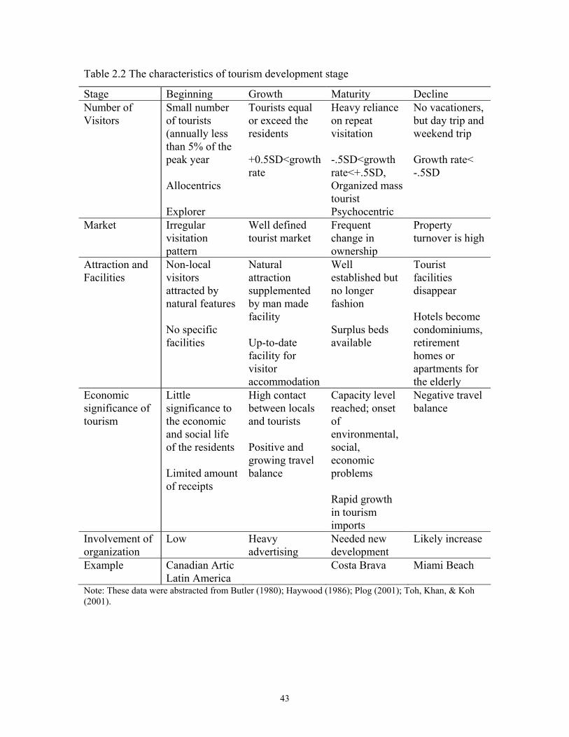
43
Table 2.2 The characteristics of tourism development stage
Stage Beginning Growth Maturity Decline Number of Visitors
Small number of tourists (annually less than 5% of the peak year Allocentrics Explorer
Tourists equal or exceed the residents +0.5SD<growth rate
Heavy reliance on repeat visitation -.5SD<growth rate<+.5SD, Organized mass tourist Psychocentric
No vacationers, but day trip and weekend trip Growth rate< -.5SD
Market Irregular visitation pattern
Well defined tourist market
Frequent change in ownership
Property turnover is high
Attraction and Facilities
Non-local visitors attracted by natural features No specific facilities
Natural attraction supplemented by man made facility Up-to-date facility for visitor accommodation
Well established but no longer fashion Surplus beds available
Tourist facilities disappear Hotels become condominiums, retirement homes or apartments for the elderly
Economic significance of tourism
Little significance to the economic and social life of the residents Limited amount of receipts
High contact between locals and tourists Positive and growing travel balance
Capacity level reached; onset of environmental, social, economic problems Rapid growth in tourism imports
Negative travel balance
Involvement of organization
Low Heavy advertising
Needed new development
Likely increase
Example Canadian Artic Latin America
Costa Brava Miami Beach
Note: These data were abstracted from Butler (1980); Haywood (1986); Plog (2001); Toh, Khan, & Koh (2001).
44
2.3.6.1. Beginning stage
Butler (1980) suggested that exploration (involvement) is characterized by small
numbers of tourists, Plog’s (2002) allocentrics, and Cohen’s (1978) explorers, who make
individual travel arrangements and follow irregular visitation patterns. From Christaller’s
(1963) model, tourists can also be expected to be non-local visitors who have been
attracted to an area by its unique or considerably different natural features. At this stage,
there would be no specific facilities provided for visitors. The physical fabric and social
milieu of the area would be unchanged by tourism, and the arrival and departure of
tourists would be of relatively little significance to the economic and social life of
permanent residents. Examples of this stage can be seen in part of the Canadian Arctic
and Latin America, to which tourists are attracted by natural and cultural historical
features. Haywood (1986) found that this stage was demarcated as years, in which the
annual number of tourist arrivals is less than 5% of the peak year. Lundtorp and Wanhill
(2001) verified Butler’s theory that during this stage, the number of tourists was below
9% of the maximum and rising moderately. Toh et al. (2001) explained the introductory
stage using travel balance, in which the primitive destination country earns a limited
amount of receipts from adventurous tourists from developed countries, resulting in a
relatively small surplus in the travel balance.
2.3.6.2. Growth stage
According to Butler (1980), the growth stage (Butler called this stage a
development stage) reflects a well-defined tourist market area, shaped in part by heavy
advertising in tourist-generating areas. As this stage progresses, local involvement and
control of development decline rapidly, and some locally-provided facilities will
disappear, being superceded by larger, more elaborate, more up-to-date facilities
provided by external organizations, particularly for visitor accommodation. Natural and
cultural attractions are developed, and the original attractions are supplemented by man-
made imported facilities. In this stage, a number of tourists at peak period probably equal
or exceed the permanent local population, and the annual growth rate is more than half
the standard deviation of annual growth rates for the entire period under study (Haywood,
1986). This stage typifies steady increases in the annual growth of tourists to a maximum,
45
whereby the location has established itself in the marketplace to the point where the
volume of tourists exceeds 50 % of the potential market (Lundtorp & Wanhill, 2001).
According to Toh et al. (2001), at this stage, a few residents from developing countries
start to travel abroad. But the rate of growth of travel exports far exceeds that of travel
imports, resulting in a positive and growing travel balance.
2.3.6.3 Maturity stage
As the area enters the maturity stage (Butler, 1980, called this stage a stagnation
stage), the peak numbers of visitors will have been reached. Capacity level for many
variables will have been reached or exceeded, with attendant environmental, social, and
economic problems. The area will be well established but it will no longer be in fashion.
At this stage, according to Haywood (1986), the growth rate of visitors is between minus
half and plus half the standard deviation of the annual growth. The type of visitor can
also be expected to move towards the organized mass type of tourist identified by Cohen
(1978) and the psychocentric type described by Plog (2001).
There will be a heavy reliance on repeat visitation and on conventions and similar
forms of traffic (Butler, 1980). Surplus bed availability and strenuous efforts will be
needed to maintain the level of visitation. Travel exports will almost peak, but the rate of
growth slows down in this stage, partly because over-development, commercialization,
and environmental pollution destroy the pristine nature of the original tourist attractions
(Haywood, 1986). At the same time, given rapid economic development and higher
income levels in newly industrialized countries, residents go abroad, resulting in
relatively rapid growth in tourism imports. During this period, the rate of growth of
tourism imports is higher than that of tourism exports, thus lowering the still-positive
travel balance (Toh, et al., 2001). The type of visitor can also be expected to change
towards the organized mass tourist identified by Cohen, and the psychocentric type
described by Plog (2001).
Natural and genuine cultural attractions will probably have been superceded by
imported artificial facilities. New development will be peripheral to the original tourist
area, and existing properties are likely to experience frequent changes in ownership. The
46
type of visitor can also be expected to change towards the organized mass tourist type
identified by Cohen and the psychocentric type described by Plog (2001).
2.3.6.4 Decline stage
Butler (1980) describes the decline stage in many ways. First, the area is not able
to compete with newer attractions and so faces a declining market, both spatially and
numerically. Second, the area no longer appeals to vacationers but is used increasingly
for weekend or day trips because it is accessible to a large number of people. Third,
property turnover is high (e.g., major tourist facilities are replaced by non-tourist related
structures, as the area moves out of tourism). Hotels may become condominiums,
convalescent or retirement homes, or conventional apartments, since the attractions of
many tourist areas make them equally attractive for permanent settlement, particularly for
elderly. Then, more tourist facilities disappear as the area becomes less attractive to
tourists and the viability of other tourist facilities becomes more questionable.
Ultimately, the area may become a veritable tourist slum or lose its tourist function
completely. However, local involvement in tourism is likely to increase at this stage, as
employees and other residents are able to purchase facilities at significantly lower prices
as the market declines. Finally, the country’s focus shifts to high-tech and value-added
industries and services with less emphasis on tourism development. Toh et al. (2001)
describes the decline stage: the wealthy travel abroad in large numbers, so that the
absolute amount of tourism imports exceeds that of tourism exports, resulting in a
negative travel balance for the country. Such trends can be seen clearly in older resort
areas in Europe. Miami Beach would also appear to be entering this stage.
The perception of various social, economic, cultural, and environmental impacts
is related strongly to the level of tourism development. Sometimes, a negative perception
of tourism development can itself be the reason that creates residents’ perceptions that
community life has declined, particularly as related to public services and opportunities
for citizens’ social and political involvement. These life conditions from tourism impact
on the community make up the life domain in general. Satisfaction or dissatisfaction
with living conditions (e.g., employment and income) from tourism impacts spill over

47
vertically to satisfactions in the life domains, and determine overall life satisfaction. The
next section addresses how tourism impacts affect residents’ major life domain and QOL
in general.
2.4. QUALITY OF LIFE STUDIES
Historically, the early attempts to measure QOL have come from the social
indicators movement (Biderman, 1974; Parke & Sheldon, 1974). The late 60’s were
officially the beginning of the social indicators movement. The U.S. Department of
Health, Education, and Welfare published two significant works, Toward the Social
Report (US Department of Health, Education, and Welfare, 1969) and Toward Social
Reporting: Next Step (Duncan, 1969). Measurement of QOL used in marketing and
related disciplines can be classified in terms of levels of analysis (Metzen, Dannerbeck &
Song, 1997). QOL can be conceived and measured at the individual level, the family
level, the community level, and the societal level. Within a given level of analysis, QOL
can be conceptualized and measured in terms of reflective or formative indicators.
Individual measurement of QOL can be classified in two dimensions: (1) subjective
versus objective indicators, and (2) reflective versus formative indicators (Figure 2.1). In
other words, the description of the measures is divided in terms of four categories:
subjective reflective indicators, objective reflective indicators, objective reflective
indicators, and objective formative indicators (Sirgy, 2001).
Reflective indicators are eccentric measures of the construct in the most
proximate fashion, and reflect a view of the construct as being unidimensional. The
societal measure of QOL involves mostly one-item measures (e.g., “On the whole, are
you very satisfied, fairly satisfied, not very satisfied, or not at all satisfied with the life
you lead? Would you say: very satisfied, fairly satisfied, not very satisfied, or not at all
satisfied?”). This measure is an example of a reflective indicator because the measure
itself is designed to capture the construct itself in a global way. The measure is not a
composite of several other measures, which in turn capture dimensions of the constructs.
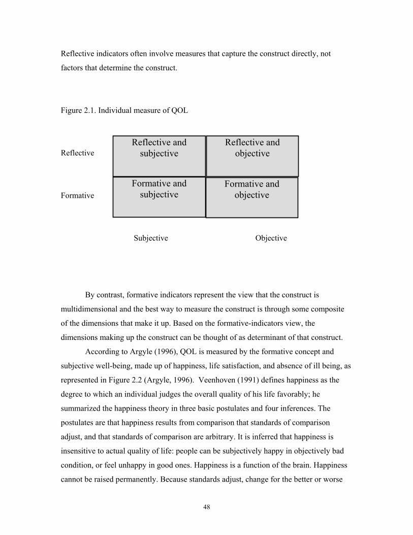
48
Reflective indicators often involve measures that capture the construct directly, not
factors that determine the construct.
Figure 2.1. Individual measure of QOL
Reflective
Formative
Subjective Objective
By contrast, formative indicators represent the view that the construct is
multidimensional and the best way to measure the construct is through some composite
of the dimensions that make it up. Based on the formative-indicators view, the
dimensions making up the construct can be thought of as determinant of that construct.
According to Argyle (1996), QOL is measured by the formative concept and
subjective well-being, made up of happiness, life satisfaction, and absence of ill being, as
represented in Figure 2.2 (Argyle, 1996). Veenhoven (1991) defines happiness as the
degree to which an individual judges the overall quality of his life favorably; he
summarized the happiness theory in three basic postulates and four inferences. The
postulates are that happiness results from comparison that standards of comparison
adjust, and that standards of comparison are arbitrary. It is inferred that happiness is
insensitive to actual quality of life: people can be subjectively happy in objectively bad
condition, or feel unhappy in good ones. Happiness is a function of the brain. Happiness
cannot be raised permanently. Because standards adjust, change for the better or worse
Reflective and subjective
Formative and objective
Formative and subjective
Reflective and objective

49
only has a short-lived effect on happiness. Happiness builds on hardship. Because
standards of comparison are anchored in earlier experience, people tend to be happier
after hard times. Happiness tends to be neutral. Because standards adjust continually,
people are typically neutral about their life, rather than positive or negative. However,
Veenhoven concluded that the overall appreciation of life (happiness) does not result
from conscious comparison exclusively, but also depends on how well we feel
affectively.
Figure 2.2. Formative QOL measure
Life satisfaction involves one’s evaluation of one’s life or life accomplishments
against some standard, e.g., achievements of significant others (Sirgy, 2001). A measure
of life satisfaction involves the following question about global evaluations of, or
feelings toward, life: how satisfied are you with your life these days? The results of a
national survey revealed that fun and family contribute more to happiness than life
satisfaction. By contrast, money, economic security, one’s house, and the goods and
services bought in the market contribute to life satisfaction more than happiness (Andrew
& Withey, 1976). Similarly, Michalos (1980) showed that evaluations of all ten measured
domains (health, financial security, family life, and self-esteem, etc.) were more closely
Happiness
Absence of ill being
Life satisfaction
QOL

50
related to life satisfaction than to happiness. Argale (1996) has argued that subjective
well-being cannot be experienced when people experience ill being in the form of
depression or anxiety. However, happiness and life satisfaction are indeed two
distinguishable constructs, one effective and the other cognitive. QOL researchers are
advised not to use the constructs of happiness and life satisfaction interchangeably
(Sirgy, 2001). Therefore, in the present study, only life satisfaction is used to measure the
QOL of the residents in the community.
Measuring QOL overall or within a specific life domain (at any level of analysis)
can be done through subjective indicators or objective indicators (Samli 1995). Objective
indicators are “hard” measures devoid of subjective assessments such as standard of
living, physical health status, and personal income, among others. Indices derived from
areas such as ecology, human rights, welfare, and education also have been sampled
frequently as social indicators. According to Diener and Suh (1997), the strength of
objective indicators is that these indicators can usually be relatively easily defined and
quantified without relying heavily on individual perceptions. For example, virtually
everyone in modern nations may agree that infant mortality is bad and that literacy is
good. Another strong point of social indicators is that by including measures across
various life domains, important aspects of society that are not sufficiently reflected in
purely economic terms can be captured. However, the largest limitation of objective
indicators is that they may not accurately reflect people’s experience of well-being
(Andrew & Withey, 1976).
On the other hand, subjective indicators are mostly based on psychological
responses, such as life satisfaction, job satisfaction, and personal happiness, etc. Despite
the impression that subjective indicators seem to be lower in scientific credibility, the
major advantage is that they capture experiences that are important to the individual. By
measuring the experience of well-being on a common dimension such as degree of
satisfaction, subjective indicators can more easily be compared across domains than can
objective measures, which usually involve different units of measurement. Diener and
Fujita (1995) provided a comprehensive review of methodological pitfalls and solutions
in the use of subjective measures of QOL. They pointed out problems associated with the
current mood of respondents, memory biases, and communication norms, among others.
51
They provided specific and constructive suggestions on the effective use of subjective
measures of QOL. For example, they recommended the use of multi-method
measurement of satisfaction, on-line sampling, varying the order of questions,
systematically manipulating the anonymity of respondents, and assessing respondents’
mood states.
Using life history methods, Parker (1997) conducted a QOL study using a
qualitative method that focuses on life history narratives to identify major factors that
influence subjective well-being. She analyzed the lives of 40 men and five women from
Cambodia, Laos, and Vietnam who re-settled in the Minneapolis/St. Paul, Minnesota
region. The results indicated that QOL of these people was influenced by their feelings of
loss of a way of life, loss of key relationships, role loss, and fears about the loss of
cultural heritage and cultural transmission to younger generations. Harvey (1997) has
argued that time-series studies can provide a valuable source of data for measuring QOL.
He maintains that time-series analysis can be applied in QOL research in relation to
traditional analysis of activity participation and time allocation. Time spent in activities
failed to predict life satisfaction among the disabled, although financial stress and social
support did.
In the present study, the measures for QOL of individuals will be representative
of subjective/reflective indicators measured by life satisfaction.
Many QOL researchers focus on the effects of many factors involved with QOL
within specific domains such as health, work, leisure, family, and community. Bubolz,
Eicher, Evers, and Sontag (1980) investigated the important quality of life domains by
using 21 Self-Anchoring Ladder of Satisfaction (SALS) items of Andrew and Withey
(1976). In the Michigan counties’ study, they found that over half of the total variance in
perceived life quality could be accounted for by only four of the variables in the SALS
scale: accomplishing something, family life, work, and financial security. Andrew and
Withey (1976) found 12 concerns, including these five, that contributed to considerable
variance: family life, work, accomplishing something, house or apartment, and fun.
Cummins, McCabe, Romeo, and Gullone (1994) and Cummins (1996) have provided
both empirical and theoretical arguments for the use of seven domains: material well-

52
being, health productivity, intimacy, safety, community, and emotional well-being.
Cummins (1997) reviewed 27 definitions of life quality that attempted to identify QOL
domains. In summary, he found that a clear majority supported five of the proposed
domains. Eighty- five percent included emotional well-being in some form (leisure,
spiritual well-being, morale, etc.), 70% included health, 70% social and family
connections (Intimacy), 59% material well-being, and 56% work or other form of
productive activity. Further empirical support for the inclusion of these five domains is
provided by data from surveys which asked respondents to indicate whether various
domains of life are important to them (Abrams, 1973; Campbell, Converse, & Rodgers,
1976; Flanagan, 1978; Krupinski, 1980). Cummins (1995) has proposed the two
additional domains of safety and community.
Cummins (1997) reviewed 32 studies and reported data on 173 different terms
that had been used to describe domains of life satisfaction. Then he classified each term
according to whether or not it could be placed within one of the seven proposed domains:
material well-being, health, productivity, intimacy, safety, community well-being, and
emotional well-being (Figure 2.3). Since these domains form the basis of the
Comprehensive Quality of Life Scale (Cummins, 1993) they will be referred to as the
ComQol domains. From the seven domains, this current study will use the particular life
domains related to tourism impacts, including material well-being, community well-
being, emotional well-being, and health and safety well-being domains. The
characteristics of each specific domain are explained in the next section.

53
Figure 2.3. Seven major QOL domains by Cummins (1997)
Emotional well-being
Community well-being
Safety
Intimacy
Productivity
Material well-being
Health
Satisfaction
54
2.4.1. Material well-being domain
Campbell et al. (1976), in the study of domain importance, reported that 73% of
the respondents scored material well-being as one of the most important domains.
Flanagan (1978) and Krupinski (1980) supported Campbell’s study that 83% of the
respondents rated the material well-being domain as important. The material well-being
domain is comprised of different components, including standard of living from
consumer well-being and income and employment from economic well-being. Each of
these components is described below.
Standard of living
According to Cummins (1996), satisfaction in the material well-being domain
mostly comes from one’s economic situation, income, living situation, standard of living,
housing, socio-economic status, financial situation, and personal possessions. This view
posits that quality of life is partly determined by satisfaction with standard of living.
Satisfaction with one’s standard living, in turn, is mostly determined by evaluations of
one’s actual standard of living compared to a set goal. Sirgy (1998) defines the material
domain as a psychological space that groups value-laden beliefs related to standard of
living. These beliefs are related to possession of material goods, wealth, and income. For
example, a person may see himself as poor in contrast to their actual situation; in other
words, people have a desired image of what they want to become or what they aspire to
be. Positive self-evaluations in the material life domain result in satisfaction with
standard of living. Belk (1988, p.291) states “Materialism reflects the importance a
consumer attaches to worldly possessions. Possessions assume a central place in a
person’s life and are believed to provide the greatest sources of satisfaction and
dissatisfaction in life.” Day (1987) and Leelakulthanit et al. (1991) conceptualized the
consumer life domain in terms of two dimensions: the acquisition and possession of
material goods. Possession of material goods refers to the collection of objects that have
monetary value (e.g., house/apartment, furniture, etc.). Meadow (1983) generated a
measure of consumer satisfaction/dissatisfaction with retail institutions for the elderly.
The measure, called the Overall Consumer Satisfaction Composite (OCSC), is based on
the theoretical notion of a satisfaction attitude hierarchy. Nakano, McDonald, and
55
Douthitt (1992) used the following instrument to measure QOL of consumer well-being.
The instrument involved questions such as, “How do you feel about your standard of
living – the things you have, like housing, car, and furniture?”
Income and employment
QOL researchers in the area of economic well-being have addressed many
questions. What is economic well-being? In all societies, more money for the individual
typically means more individual happiness. However, Duncan (1975) argued on the basis
of studies of happiness in some 19 countries, that raising incomes of all people does not
increase the happiness of all people. In explanation of this conclusion, Esterlin (1973)
observed that individuals assess their material well-being, not in terms of the absolute
amount of goods they have, but relative to a social norm of what goods they ought to
have. Subjective indicators of economic well-being typically involve any one or
combination of the following constructs: income satisfaction and feeling of financial
security and satisfaction (Andrew & Withey, 1976). Andrew and Withey (1976)
measured economic well-being in terms of people’s feelings regarding how secure they
are financially, their family income, and how well off they think they are.
The money index was found to be a significant and strong predictor of life
satisfaction. Previous research has also shown that income plays a significant role in the
perception of QOL (Campbell, 1981), although it may not be the most important factor.
Veenhoven (1991) calculated the covariation between income and happiness across
countries or regions of the world, and he found strong correlations of 0.51, 0.59 and 0.84
across several different data sets. He also found that the income and subjective well-
being relation was significant in all of the analyses at two points in time, indicating that
income is a resource that does covary with well-being.
However, there were no social comparison, adaptation, or expectancy effects
found, and the results generally were in the opposite direction from those predicted by
the relative approach. Diener (1994) has shown that happiness levels in the U.S.A.,
France, and Japan has not changed since World War II, despite rapid economic growth in
these countries. Duncan (1975) showed that no aggregate change in satisfaction with the
standard of living occurred over a 16-year period. He showed that the mean satisfaction
56
score was 2.47 in 1971 and 2.41 in 1955 in the Detroit, Michigan Area. The difference of
0.06 produces a t-statistic of 1.20, p=0.23, which is a non-significant value. This result
was emphasized because data on income collected from the same respondents leave little
doubt that material levels of living were in fact higher in 1971 than in 1955. The median
family income reported in the 1955 survey was $5,827 as compared with $12,407 in
1971. Over this period, however, the consumer price index for Detroit (1967=100) rose
from 82.2 to 127.7 (U.S. Bureau of the Census, 1974); hence, the 1955 dollar was worth
1.5 times as much as the 1971 dollars. Expressing 1955 median family income in 1971
dollars, Duncan obtained $8,740, so that the median income in constant dollars increased
by a factor of 1.42 over this period. Thus, the proposition in Easterlin’s conclusion is
strongly confirmed; increasing the standard of living in real terms does not lead to a
subjective increase in the standard of living for the population as a whole. Therefore, the
relationship between economic well-being is construed and operationalized through
subjective indicators or objectives. Support for the effect of economic well being on
overall QOL comes from studies employing subjective indicators only.
Lane (1991) emphasized that people who succeed in the labor market tend to
attribute their financial success to themselves, and thus feel proud of their
accomplishments. These feelings of pride and personal control play a significant role in
general feelings of life satisfaction. Gerlach and Stephen (1997) have conducted a
comparative analysis of East versus West Germany. The study indicates that
unemployment is higher in East than West Germany. By contrast, subjective well-being
is lower in East Germany than in West Germany. The authors conclude that
unemployment plays a significant role in subjective well-being. Work plays an important
role in subjective well-being. Lane (1991) also argues that subjective well-being affects
financial well-being. This is because those who feel happy about life in general tend to
work harder, and thus generate more income. Good management of financial resources
paves the way to higher levels of economic well-being and life satisfaction.
57
2.4.2. Community well-being domain
Many public policy makers interested in regional economic development have
become increasingly interested in broadening the concept of economic development to
socio-economic development. In doing so, they have begun to use social indicators in
assessing QOL of a given region or community. Community QOL plays a significant role
in overall QOL. From the viewpoint of community residents, the overall findings from
QOL research point to the importance of information communicated through the local
media, perception of safety and crime, and community beautification programs. Also
Cummins (1997) found that the satisfaction associated with the community well-being
domain occurs when people achieve satisfaction with education, neighborhood, service
and facilities, social life and social relations.
Norman, Harwell, and Allen (1997) conducted a study showing that community
satisfaction does make a significant and positive contribution to community residents’
perceptions of their own quality of life. The study involved five rural South Carolina
communities. The sample involved 360 residents who responded by completing a survey
questionnaire. The study revealed that satisfaction with recreational services provided by
the town does positively affect community satisfaction. In 1995, Wagner, with the
regional plan association and the Quinnipiac College Polling Institute of Hamden, New
Jersey, examined the determinants and consequences of perceived community QOL in
New York, New Jersey, and Connecticut. The study also surveyed 400 people from each
of four other major metropolitan areas, namely Los Angeles-Riverside-Orange County,
Dallas/Forth Worth, Atlanta, and Seattle-Tacoma-Bremerton. The results of this survey
indicated that a person’s satisfaction with their community has a big effect on their
perceived QOL. Sirgy and Cornwell (2001) extended and refined Sirgy et al.’s (2000)
study. The modified study found that satisfaction with community at large is mostly
determined by satisfaction with government service, business service, non-profit service,
as well as satisfaction with other aspects of community (e.g. quality of environment, rate
of change of natural landscape, etc.).
Another factor that may affect overall life satisfaction through its impact on a
community is an individual’s perception of the quality of public services. Studies by
58
O’Brian and Lange (1986) and Schuman and Gruenberg (1972) have shown assessments
of the satisfaction of the service quality on community for some residents can be found.
Similarly, the availability and use of retail service may affect life satisfaction through
related impacts on community. Some studies have shown that the use of real facilities in
a community increases a sense of community (e.g., Roach & O’Brian, 1982).
2.4.3. Emotional well-being domain
When Cummins (1997) reviewed the 32 studies and classified 173 different terms
into seven proposed domains, the satisfaction of emotional well-being domain mostly
came from leisure activities, religion, recreation, and hobbies. He found that 85% of the
studies included emotional well-being in some form of leisure, spiritual well-being,
morale, etc. Flanagan (1978) and Krupinski (1980) asked respondents to rate domain
importance. Eighty-six percent of the respondents for both studies ranked emotion well-
being in the top two categories (important/very important). Also most of respondents
answered that the satisfaction of emotional well-being comes from spiritual and leisure
activities. Therefore, the present study adopts leisure and spiritual activities as
components of the emotional well-being.
Leisure activity
Leisure has been defined in terms of discretionary time use: a person
experiencing leisure is using the time remaining after work is completed. Thus, leisure is
total time minus time spent on non-discretionary activities (Gerstl 1983; Page-Wood,
Lane, & Lindquist 1990; Vickerman 1980). This definition of “leisure” is grounded in
traditional economic theory, which divides human activities in terms of time spent on
production, consumption, and leisure. QOL researchers have conceptualized leisure well-
being in terms of: leisure satisfaction (e.g., Neal, Uysal, & Sirgy 1995, 1999: Norman,
Harwell, & Allen 1997); leisure-life experience-construed and measured in terms of
leisure boredom (e.g., Haggard, Granzin, & Painter, 1995); satisfaction with non-working
activities (e.g., Campbell et al. 1976); amount of fun one is having (e.g., Andrews &
Withey, 1976); things done with family (e.g., Andrew & Withey, 1976); time to do things
59
(e.g., Andrew & Withey, 1976); spare time activities (e.g., Andrew & Withey, 1976);
and leisure experience in terms of peace, achievement, exercise, and risk (e.g., Unger &
Kernan, 1990).
Leisure is an important source of subjective well-being. A study by Veroff et al.
(1981) found that 34% of people in jobs find leisure equally as satisfying as work, and
19% find it more satisfying. Orman, Harwell, and Allen (1997) have conducted a study
showing that leisure satisfaction in one’s community does make a significant and positive
contribution to community residents’ perceptions of their quality of life. The study
involved five rural South Carolina communities. The sample included 360 residents who
responded by completing a survey questionnaire. Haggard, Granzin, and Painter (1995)
conducted a study on a sample of 513 adults to investigate the relationship between
leisure-life experience (construed and measured in terms of leisure boredom) and QOL.
The data indicated that leisure-life experience does influence QOL but its effect is
indirect, through an intervening variable such as mental health.
Neal, Uysal, and Sirgy (1995, 1999) have shown empirically that leisure
satisfaction plays a significant role in affecting life satisfaction; they have developed a
conceptual model that captures the relationship among satisfactions with various aspects
of tourism, leisure, and overall life. Leisure satisfaction has two main derivatives: leisure
satisfaction experienced at home and away from home. Leisure satisfaction experienced
away from home comes from essentially two sources: satisfaction with travel and tourism
services, and satisfaction with own travel efforts. Finally, satisfaction with travel and
tourism service comes from satisfaction with travel pre-trip services, satisfaction with
travel trip route services, and satisfaction with travel destination services. Campbell et
al. (1976) showed that satisfaction with non-working activities contributes approximately
29% variance accounted for in life satisfaction, the greatest amount of variance
controlling for the effects of family life, standard of living, savings and investments,
work, marriage, friendship, and housing.
There are many factors affecting leisure well being. Examples of significant
factors are: time with significant other; preference for activities having skill, identity,
autonomy; and differences in allocentricism and psychocentrism (individual difference
factor). Staats, Partlo, Holzapfel, and Miller (1992) have examined family patterns in use
60
and wished-for use of free time. They conducted a survey using college students and their
parents. The study reveals that most people spend most of their leisure time with family
and friends and that they desire to do so, too. The implication of this finding for
marketers of leisure goods and services is to design such goods and services to enhance
family/friends’ interactions. Argyle and Lu (1990) conducted a study of 39 leisure
activities and found that these activities fall into at least two major categories such as
teams and clubs, dances, parties, debates, and meeting new people. Neal, Sirgy, and
Uysal (1995) have conducted a study of 373 consumers of travel/tourism services
employed in a major state university to examine differences between allocentrics and
psychocentrics in their satisfaction with leisure life and various aspects of travel and
tourism services. Psychocentrics are travelers who are self-inhibited and non-
adventuresome on vacation. Allocentrics, on the other hand, are those who enjoy trying a
wide variety of pursuits and challenges while on a vacation. The study results indicate
that the more allocentric a traveler is the more she or he is likely to be satisfied with
destination services, travel services in general, trip experiences, perceived freedom from
control, perceived freedom from work, involvement, arousal, spontaneity, leisure
experience at home, and leisure life in general.
Spiritual (religious) activity Researchers have defined this concept in various ways. One popular definition of
spiritual well-being is the satisfaction one feels in relation to one’s conception of his or
her God (e.g., Paloutzian and Ellison 1982). Another definition includes the extent to
which one finds meaning and purpose in life (Ellison 1983). Paloutzian (1997) has
argued that spiritual well-being does play a significant and positive role in subjective
well-being. A literature review of studies in this area reveals that spiritual well-being is
positively related to purpose in life, coping with terminal illness, adjustment to
hemodialysis; this variable is negatively related to anxiety, depression, and other
psychological and health related variables. The spiritual well-being measure was
originally developed by Paloutzian and Ellison (1979, 1982) and re-tested by Brinkman
(1989), Bufford et al. (1991), Ellison (1983), and Scott, Agresti, and Fitchett (1998). This
is a 20-item self-report measure in which responses were recorded on a 6-point scale
61
ranging from strongly disagree to strongly agree (e.g., I don’t find much satisfaction in
private prayer with God, or I don’t know who I am, where I came from, and where I’m
going, etc.). Scott, Agresti and Fitchett (1998) factor analyzed these items and showed
that there are three factors imbedded in this measure, namely affiliation (6 items),
alienation (6 items), and dissatisfaction with life (3 items).
2.4.4. Health and safety well-being domain
From the ecology, Bubloz et al. (1980) addressed QOL, using concepts of the
human environed unit, the environment, and the interactions. A “human environed unit”
is a social unit placed in an environmental context. The environment is the place that
provides energy and matter (resources) for sustenance of the human environed unit. The
interactions involve interrelationships among the components of the human environed
unit, among the components of the environment, and/or between the units and the
environment. From this perspective, QOL is viewed as a high need satisfaction across life
domains. Thus, the environment should be preserved and enhanced to provide sufficient
resources to meet those needs of the human units within it. Also, for a number of reasons,
including interest in the social determinants of health, the impact of Healthy Cities and
Health Communities movements, and growing concern with consumer’s view of health
and social service resources and provision, more attention is being directed to
environmental indicators of quality of life (Raphael, Renwick, Brown, & Rootman,
1996).
Much research has shown that feelings about personal health spill over to overall
life satisfaction, because personal health is considered important in one’s evaluation of
life (Andrew & Withey 1976). For example, Maddox and Douglass (1978) have shown
that the healthier an elderly person feels, the more likely he or she is to be satisfied with
life in general. However, the subjective belief that one is healthy or ill may be more
important than the actual medical status in predicting an individual’s general emotional
status and behavior. Maddox and Douglass (1978) also investigated the relationship
between the self and the health ratings of the individual by their physician. In their
experiments, in all observations, the panel of older persons tended to present congruous
62
responses. The first hypothesis, that the subjective belief that one is healthy or ill may be
more important than one’s actual medical status, is supported. When incongruity is
observed, there will be over-estimation of health more likely than under-estimation.
Walker, Lee, and Bubolz (1990) have shown that the number of health symptoms is
significantly related to overall QOL and marital happiness. Okun et al. (1984) performed
a meta-analysis of 104 studies published before 1980 focusing on the American elderly
and concluded that objective and subjective measures of health account for 8-14% of the
variance in subjective well being.
Rahtz, Sirgy, and Meadow (1989) explored the role of personal health on the
relationship between community healthcare satisfaction and life satisfaction among the
elderly. The study revealed a stronger relationship between community healthcare
satisfaction and life satisfaction when personal health is perceived as poor (as compared
to good). Sirgy et al. (1995) conducted another study to investigate the mediating versus
moderating roles of personal health satisfaction on the spill over effect of community
health care satisfaction on life satisfaction. The results indicated that personal health
satisfaction is a mediator between community healthcare satisfaction and life satisfaction
for a general population involving elderly, and the results indicate a moderation effect.
There are many measures of health-related QOL. Example measures include the
Barak, and Rahtz Measure of Health Satisfaction (1990) which contains the following
items: “I never felt better in my life; My health is just beginning to be a burden; I still
feel young and full of spirit; I am perfectly satisfied with my health.” Responses to these
statements were recorded on a 5-point scale varying from “strongly disagree” to
“strongly agree,” and the study produced a reliability coefficient of .70.
2.4.5. Other well-being domains
Family well-being
There is much evidence suggesting that family QOL does play a significant role
in the overall QOL. For example, Andrew and Withey (1976) found family well-being to
be a significant predictor of life satisfaction, controlling for the effect of efficacy, money,
amount of fun one is having, house/apartment, things done with family, time to do things,
63
spare-time activities, recreation, national government, and consumer. Western (1997)
conducted a study involving 2,850 young people (aged 11 to 19 years) and their parents
in Australia. The major finding of this study related to QOL is that satisfaction with
relationships within the family is a strong predictor of subjective well-being for both
adolescents as well as parents.
Examples of measures of family QOL at the individual level of analysis (not the
family level) include the Perceptual Indicators of Family Life Quality (PIFQ) measure
and the Kansas Family Life satisfaction measure. Retting and Leichtentritt (1997)
developed the Perceptual Indicators of Family Life Quality (PIFQ) scale. The measure is
theoretically grounded in resource theory. It involves items related to six resources: love,
status, services, information, goods, and money. The individual’s evaluation of family
life essentially reflects the degree to which the family environment satisfies personal
needs for love and affection (love), respect and esteem (status), comfort and assistance
(service), communication resulting in shared meaning (information), ownership of
personal things (goods), and money for personal use (money). The combination of family
well-being scores from several family members indicates family QOL. A study was
conducted involving 560 adults, and the results provided some validation support, mostly
form the women’s data. Walker, Lee, and Bubolz (1990) have used the Kansas Family
Life Satisfaction Scale (Schumm et al. 1986). This measure consists of four statements
regarding satisfaction with family, relationship with spouse, relationship with children,
and children’s relationships with each other. Responses to these statements were recorded
on a 7-point scale varying from “completely dissatisfied” to “completely satisfied”.
Neighborhood well-being
The neighborhood community may affect overall life satisfaction in its role as an
intervening variable through which residents’ experiences of other neighborhood
conditions come to affect their assessments of their lives in general. For example, it has
been argued that the presence of crime in a neighborhood not only affects individuals
directly through an increase in fears about their safety, but also reduces their interaction
with one another and seriously impedes the development and/or maintenance of
community at the local level (Wilson, 1975). If the preceding assertions about the
64
importance of neighborhood community in individuals’ lives are correct, then the
experience of victimization in a neighborhood is likely to have a specific and measurable
negative impact on overall subjective quality of life through its weakening of the bonds
of community that individuals’ sense regarding attachment to his or her community.
Widgery (1995) conducted a study in which he measured QOL of a community through a
self-report (subjective) instrument of community residents. Community residents were
asked to indicate their satisfaction with eight aspects of neighborhood life: overall
neighborhood quality, neighbors, home, aesthetic quality, government services, racial
mix, school, and security from crime.
2.5. CHAPTER SUMMARY
This chapter defines the constructs to be studied based on the conceptualization
and previous empirical and theoretical studies. While there could be other factors (the
elements of tourism impacts or well-being domains) that would affect life satisfaction in
general, it is believed that this study has incorporated the relevant variables necessary to
answer the four questions stated in Chapter I.
First, this chapter explains the relevance of this research; in the second section, it
reviews the concept of carrying capacity, tourism life cycle with an explanation of the
characteristics of different stages, and their interrelationships with tourism impacts and
residents’ QOL. The third section addresses residents’ perception of tourism impacts,
explaining its four dimensions from marketing, recreation, and consumer behavior fields.
The last section presents particular life domains of the quality of life of residents. The
next chapter provides a summary of research hypotheses and discusses research design
and methodology in detail. The items that are going to be used to measure each construct
are also discussed in a brief manner.

65
CHAPTER THREE
RESEARCH METHODOLOGY
3.1 INTRODUCTION
This chapter defines the study’s research problems and explains the framework of
the research. Research propositions and hypotheses are discussed at great length. A
description of the survey instrument and a discussion regarding the development of
survey questions is given. Data collection and methods of statistical analyses are
discussed. The final section addresses the issues of reliability and validity of
measurement scales.
3.2 RESEARCH FRAMEWORK
There were four research questions addressed by this study, as stated in Chapter I.
The first was to examine the influence of tourism impact on QOL of residents in the
community. Perceived tourism impact was found to have four dimensions: economic,
social, cultural, and environmental. The second research question was to determine the
influences of tourism impact on the particular life domains. The particular life domains
were tested as having four domains: material well-being, community well-being,
emotional well-being, and health and safety well-being. The third research question was
to investigate the influence of the particular life domains on overall life satisfaction of the
residents in the community. The final research question was to determine the influences
of tourism development stages on the relation between tourism impact dimensions and
the particular life domains. The tourism development stage was divided into four
different stages: beginning, growth, maturity, and decline stages. Figure 3.1 presents the
theoretical model and the hypotheses in this study. The next section of this chapter
presents the study hypotheses.
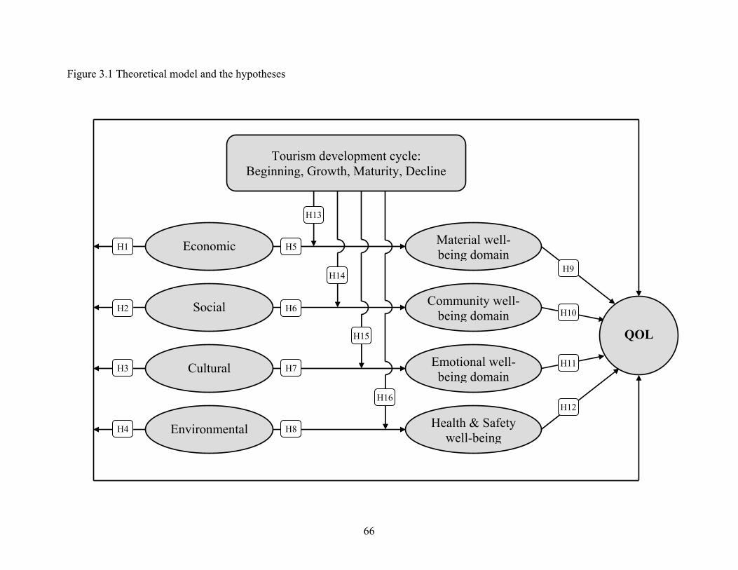
66
Figure 3.1 Theoretical model and the hypotheses
Emotional well-being domain
Economic Material well-being domain
Social
Cultural
Environmental
Community well-being domain
Tourism development cycle: Beginning, Growth, Maturity, Decline
Health & Safety well-being
H5
H6
H7
H8
H9
H10
H11
H12
H13
H1
H2
H3
H4
QOL
H14
H15
H16
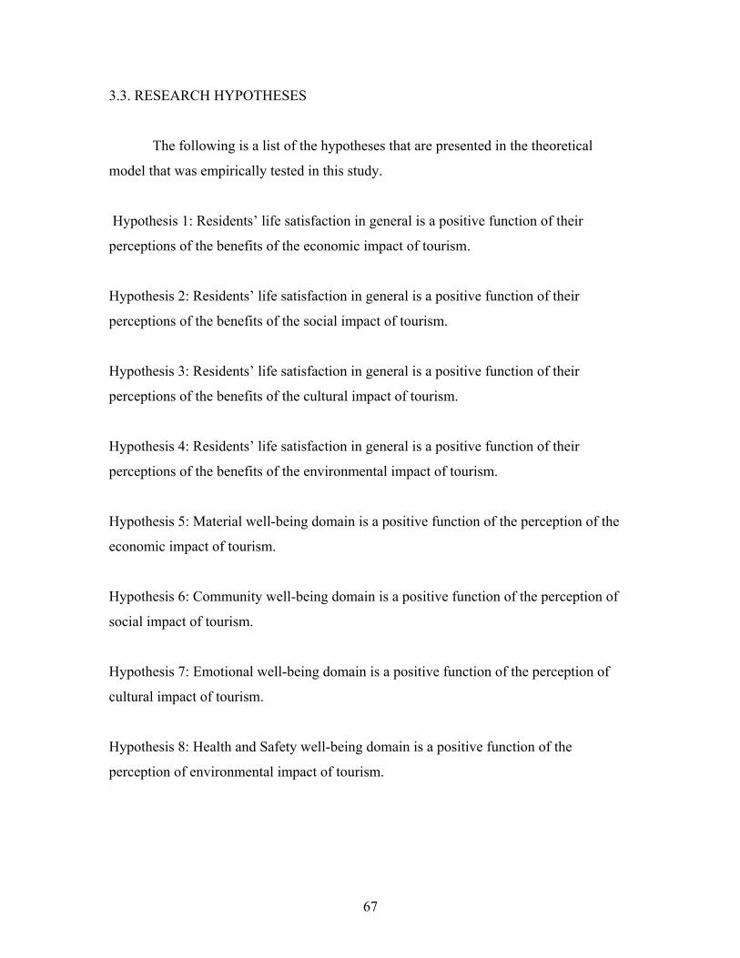
67
3.3. RESEARCH HYPOTHESES
The following is a list of the hypotheses that are presented in the theoretical
model that was empirically tested in this study.
Hypothesis 1: Residents’ life satisfaction in general is a positive function of their
perceptions of the benefits of the economic impact of tourism.
Hypothesis 2: Residents’ life satisfaction in general is a positive function of their
perceptions of the benefits of the social impact of tourism.
Hypothesis 3: Residents’ life satisfaction in general is a positive function of their
perceptions of the benefits of the cultural impact of tourism.
Hypothesis 4: Residents’ life satisfaction in general is a positive function of their
perceptions of the benefits of the environmental impact of tourism.
Hypothesis 5: Material well-being domain is a positive function of the perception of the
economic impact of tourism.
Hypothesis 6: Community well-being domain is a positive function of the perception of
social impact of tourism.
Hypothesis 7: Emotional well-being domain is a positive function of the perception of
cultural impact of tourism.
Hypothesis 8: Health and Safety well-being domain is a positive function of the
perception of environmental impact of tourism.

68
Hypothesis 9: Residents’ life satisfaction in general is a positive function of material
well-being domain.
Hypothesis 10: Residents’ life satisfaction in general is a positive function of community
well-being domain.
Hypothesis 11: Residents’ life satisfaction in general is a positive function of emotional
well-being domain.
Hypothesis 12: Residents’ life satisfaction in general is a positive function of health and
safety well-being domain.
Hypothesis 13: The relationship between economic impact of tourism and material well-
being is strongest in relation to the beginning and growth stages of the tourism
development cycle and weakest in relation to the maturity and decline stages.
Hypothesis 14: The relationship between social impact of tourism and community well-
being is strongest in relation to the maturity and decline stages of the tourism
development cycle and weakest in relation to the beginning and growth stages.
Hypothesis 15: The relationship between cultural impact of tourism and emotional well-
being is strongest in relation to the maturity and decline stages of the tourism
development cycle and weakest in relation to the beginning and growth stages.
Hypothesis 16: The relationship between environmental impact of tourism and health and
safety well-being is strongest in relation to the maturity and decline stages of the tourism
development cycle and weakest in relation to the beginning and growth stages.
3.4. STATISTICAL METHOD EMPLOYED
The study adopts two different multivariate data analysis techniques to test the
proposed model, consisting of two phases. The first phase focuses on the testing from the
hypothesis 1 to hypothesis 12 for the proposed antecedents and consequences of tourism
impacts, particular life domains, and overall quality of life. The second phase focuses on
examining the proposed moderating effects of tourism development stage on tourism
impact dimensions and its associated consequences, the particular life domains.
3.4.1. Phase I: Structural equation modeling
Structural equation modeling (SEM) was utilized to empirically test the
relationships between the constructs in this study. SEM allows simultaneous estimation
of: 1) a measurement model that relates the observed indicators in each scale to the
construct they represent, giving factor loadings for each observed indicator; and 2) a
structural model that relates constructs to one another, providing parameter values (i.e.,
path coefficients). This method was chosen so that both a model accounting for
measurement error in the constructs and their respective scale measurements, and
simultaneous estimation of those relationships for the complex model can be achieved
(Anderson & Gerbing, 1988). The properties of the observed indicators of the constructs
in the proposed model and the hypotheses was tested using the LISREL 8 structural
equation analysis package (Jöreskog & Sorbom, 1993) with the maximum likelihood
(ML) method of estimation (Anderson & Gerbing, 1988; Bentler, 1983), in combination
with the two-stage process recommended by Anderson and Gerbing (1988) and Sethi and
King (1994). More specific discussion is presented in the next section.
3.4.1.1. Measurement model
First a confirmatory measurement model that specifies the posited relationships of
the observed variables to the underlying constructs, with the constructs allowed to
intercorrelate freely was tested as recommended by Sethi and King (1994), and Anderson
and Gerbing (1988), and Jöreskog (1993). They recommend the use of a measurement
model to separate measurement issues from model structure issues. Use of confirmatory
69
factor analysis (CFA) ensures the unidimensionality of the scales measuring each
construct in the model. It also avoids interaction of the measurement and structural
models that could affect the parameters associated with the hypothesized relationships
between the constructs in the model. Therefore, before testing the overall measurement
model, the measurement unidimensionality of each construct is assessed individually
(Sethi & King, 1994). This present study used at least three indicators to measure one
construct. Constructs with unacceptable fits (lower than 0.7 of factor loading) are
respecified by deleting the indicators that did not work out as planned to have a
unidimensional measurement (Anderson & Gerbing, 1988).
After assessing the unidimensionality of each construct individually (Sethi &
King, 1994), a measurement model for each pair of constructs was estimated, combining
them two by two (Jöreskog, 1993). First, each construct’s fit is measured. After making
sure that the fit of each construct is acceptable, the fit of two constructs (a pair) is
measured. All constructs are paired with each other. For example, assume that we have
three constructs, A, B, and C. First, constructs are paired as AB, AC, BC (all possible
pairs). Afterwards, each pair of constructs’ fit is measured separately to make sure that
indicators of each construct do not load on other constructs. Then the overall
measurement model fit is tested (Anderson & Gerbing, 1988; Jöreskog, 1993; Sethi &
King, 1994).
As fit indices, the chi-square statistic (and associated p values) is examined first.
The model is deemed acceptable if the chi-square value is less than three times the degree
of freedom (Carlmines & McIver, 1981). However, as noted by Jöreskog (1993, p.309)
“since chi-square is N-1 times the minimum value of the fit function, the chi-square test
tends to be large in large samples.” Because of the large effect of sample size on the chi-
square values (and associated p values), other fit indices are also selected to measure the
fit of the tested models based on the recommendations of several researchers from a
number of different disciplines. These selected fit indices are the standardized root-mean
square residual (SRMR), the incremental fit index (IFI; Bollen, 1989), the parsimonious
normed-fit index (PNFI; Mulaik, James, Alstine, Bennet, Lind & Stilwell, 1989), the non-
normed-fit index (NNFI; Hu & Bentler, 1995), the comparative fit index (CFI; Bentler,
1990) and the root mean squared error of approximation (RMSEA: Hu & Bentler, 1999).
70
The values of IFI, PNFI, NNFI, and CFI range from zero to one, with a value close to 1.0
indicating a good fit. SRMR and RMSEA also range from zero to one, with a value close
to 0.0 indicating a good fit (e.g., Byrne, 1989; Mulaik et al, 1989). Hu and Bentler (1999)
suggested that, for the ML method, a cutoff value close to 0.95 for NNFI, IFI, CFI, and
RNI (for all these, Hair et al. (1998) suggested that cutoff value of .8 is marginally
acceptable level in social science); a cutoff value close to 0.08 for SRMR; and a cutoff
value close to 0.06 for RMSEA are needed to conclude there is a relatively good fit
between the hypothesized model and the observed data.
The principal advantages of the overall model fit measures are that they evaluate
the whole model and they can indicate inadequacies not revealed by the fit of model
components (e.g., equations and parameter estimates). One limitation is that they are
inapplicable to an exactly identified model, and a second limitation is that overall fit
measures can differ from the fit of components of the model. For example, the overall fit
may be good, but parameter estimates may not be statistically significant or may have
signs opposite to that predicted. And conversely, in many cases, component fit may
suggest adequate fit while the overall measures of fit suggest an inadequate model. For
these reasons the overall fit measures should not be used in isolation from the component
fit measures, such as parameter estimates, asymptotic standard error (problem if it is
greater than 2) and asymptotic correlation matrix of parameter estimates (Bollen, 1989).
All the parameter estimates should be considerably larger (i.e., generally + or – 2) than
their standard errors and high correlations sometimes between indicators are a symptom
of severe collinearity. Usually a correlation over 0.7 can be considered large.
3.4.1.2. Structural equation model
The structural portion of the SEM allows for the testing of multiple equations
with multiple dependent variables. This statistical method provides parameter values (i.e.,
path coefficients) for each of the research hypotheses and determines their respective
significance. As recommended by Anderson and Gerbing (1988) for assessing the
structural model in a two-step approach, a series of five nested structural models are first
tested to identify the best structural model that fits the data. A nested model is one in
which a simpler model is nested, within another (more complex) model. The first model
71
is the null structural sub-model (Mn) in which all parameters relating the constructs to
one another are fixed at zero. The second model is the theoretical model (Mt) that
estimates all parameters relating the constructs to one another. From a theoretical
perspective, the constrained model (Mc) is the next most likely model. It is similar to the
theoretical model (Mt) except that one or more parameters estimated in Mt are fixed zero.
The next most likely model, from a theoretical perspective, is the unconstrained
alternative model (Mu) in which one or more parameters constrained in Mt are estimated.
In the unconstrained model, all paths proposed in the theoretical model were estimated. A
saturated structural sub-model (Ms) can be defined as one in which all parameters
relating the constructs to one another are estimated. Before testing all nested models,
each structural model is assessed to see if it has an acceptable goodness of fit, as
recommended by Anderson and Gerbing (1988) and Bentler and Bonett (1980). A pseudo
chi-square test is utilized (Bentler & Bonett, 1980) in which a pseudo chi-square statistic
is constructed from the chi-square value for any structural model (Ms) (the smallest chi-
square value possible for any structural model) with the degrees of freedom from the null
structural sub-model (Mn) (the largest number of degrees of freedom for any structural
model). An insignificant pseudo chi-square test indicates that one or more structural
models are likely to give acceptable fit. On the other hand, a significant pseudo chi-
square test indicates that no structural model would give acceptable fit, because it would
have a chi-square value greater than or equal to the value for the saturated model (Ms)
with fewer degrees of freedom than for the null structured sub-model (Mn). However,
one should remember that pseudo chi-square values tend to be large in large samples and
complex models because the pseudo chi-square value is calculated based on the chi-
square value. Therefore, caution is advised when assessing the fit of any model based on
the results of the pseudo chi-square test, especially when the sample size exceeds 200 and
when the model is complex. Researchers suggest that other fit indices should also be
utilized in the present study to assess the fit of any model. As stated earlier, other fit
indices are utilized to measure the fit of the tested models. These selected indices are the
goodness-of-fit index (GFI), the adjusted goodness-of-fit (AGFI: Bentler, 1983), the
standardized root-mean square residual (SRMR), the incremental fit index (IFI), the
parsimonious normed-fit index (PNFI), the non-normed-fit index (NNFI), the
72
73
comparative fit index (CFI), and the root mean squared error of approximation
(RMSEA). Each of the goodness of fit index is explained in Chapter IV in a detailed
manner.
3.4.2. Phase II: Hierarchical multiple regression
The second phase focuses on examining the moderating effects of tourism
development stages on the relationship between tourism impact dimensions and particular
life domains. The basic premise of these moderating effects is that responses to variation
in the satisfaction of the particular life domains resulting from the degree of the
perceptions of the tourism impact depend on the tourism development stages of the area.
Zedeck (1971) described the moderating effect by stating that Z is a moderator of the
relationship between variable X and Y when the nature (i.e., magnitude) of this
relationship varies across level of Z.
The most widely used statistical procedure to estimate moderating effects is
hierarchical multiple regressions (HMR). HMR can detect the moderating effects for
moderator variables that are measured on both continuous and dichotomous scales
(Cohen & Cohen, 1983). HMR is favored by researchers over other statistical techniques,
such as the comparison of sub-group based correlation coefficients for two or more sub-
groups, and HMR analysis provides researchers with important information about slope
differences for various sub-groups (Aguinis & Stone-Romero, 1997). Specially, an
interaction, u x v = uv, where u is a dichotomy and v a quantitative variate, is
interpretable as a slope difference between the groups in their Y on v regression lines
(Cohen & Cohen, 1983, p. 317). Therefore, the study uses the HMR to examine the
presence of moderating effects. Following the procedure articulated by Cohen and Cohen
(1983), the dependent variables (i.e., material well-being) are regressed on the
independent variable (i.e., economic impact of tourism) and moderator (tourism
development stage). Next, the cross-product vector of the independent variable and the
moderator are computed and added to the equations. A significant beta weight for the
interaction term indicates that the moderator moderates the relationship between the
independent variable and the dependent variable. A negative regression coefficient for the
74
interaction term signals that the relationship between the independent variable and the
dependent variable is stronger at lower levels of the moderator than higher levels of the
moderator.
3.5. RESEARCH DESIGN
3.5.1. Survey Instrument
The survey instrument consisted of three sections. The first two sections consist
of items that utilize a 5-point Likert type scale. The anchors include: a) very dissatisfied
to very satisfied and b) strongly disagree to strongly agree. The third part of the
questionnaire gathered demographic information on residents in communities.
3.5.2. Data collection
A self-administered survey questionnaire was used to collect data. The
questionnaire was stamped with sequential numbers and delivered via the U.S. Postal
service to randomly stratified samples (explained in the next section) of Virginia
residents. Several measures were employed in an effort to increase response rate. A cover
letter that was signed individually in blue ink and contained the name and address of the
respondent was attached to each questionnaire in an attempt to show personalization. A
self-addressed, stamped envelope was included in the package being mailed. Two weeks
after the survey was mailed, a reminder postcard was sent to those who have not returned
their survey (Dillman, 1978). Last, another two weeks after the reminder postcard was
mailed; the second survey questionnaire was mailed those who had not returned their
survey.
3.5.3. Sample
The sample for study included residents in selected regions of Virginia who were
at least 19 years of age or older. First, the areas for each tourism development stage was
selected by using four secondary indicators, then a stratified sampling method was
75
utilized to determine the number of respondents required from each county and city of
Virginia for each development stage. Afterwards, random sampling was used to select a
predetermined number of respondents from each county and city of Virginia. The sample
(mailing list) for this study was obtained from Reference USA data
(http://www.referenceusa.com/) in the residential information section. Reference USA’s
residential information is compiled from more than 3,900 white page telephone
directories. Each listing appears in the database exactly as it appears in the phone book.
Reference USA data does not include unlisted phone numbers.
The selection procedure of areas for development stage and stratified random sampling
First, to select the area to fit each tourism development stage, four types of
secondary data investigated by the Virginia Tourism Beaurue were used. These
secondary data (indicators) were selected based on the review of tourism development
research literature. According to the results of Perdue et al. s’ (1991) study, four
significant secondary indicators from 1990 to 2000 were chosen and adopted: Population
Growth Rate (PGR), Traveler Spending Growth Rate (TSGR), Direct Travel
Employment Growth Rate (DTEGR), and State Travel Tax Growth Rate (STTGR). Then
a modified criterion from Toh, Khan, and Koh (2001) was used to select the best place
for each development stage.
Toh et al. (2001) expanded Haywood’s (1986) criteria into the indicator of
international destination life cycle. By using the standard deviation of the country’s travel
balance, Toh et al. (2001) found that Singapore is about to enter the decline stage. They
postulated that in the beginning stage, the primitive destination country earns a limited
amount of receipts from adventurous tourists from developed countries. In the growth
stage, a few residents from developing countries start to travel abroad, but the rate of
growth of travel exports far exceeds that of travel imports, resulting in a positive and
growing travel balance. In the maturity stage, the rate of growth of tourism imports is
higher than that of tourism exports, thus lowering the still positive travel balance. Finally,
in the decline stage, the wealthy travel abroad in large numbers so that the absolute
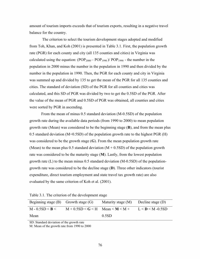
76
amount of tourism imports exceeds that of tourism exports, resulting in a negative travel
balance for the country.
The criterion to select the tourism development stages adopted and modified
from Toh, Khan, and Koh (2001) is presented in Table 3.1. First, the population growth
rate (PGR) for each county and city (all 135 counties and cities) in Virginia was
calculated using the equation: (POP2000 – POP1990 )/ POP1990 - the number in the
population in 2000 minus the number in the population in 1990 and then divided by the
number in the population in 1990. Then, the PGR for each county and city in Virginia
was summed up and divided by 135 to get the mean of the PGR for all 135 counties and
cities. The standard of deviation (SD) of the PGR for all counties and cities was
calculated, and this SD of PGR was divided by two to get the 0.5SD of the PGR. After
the value of the mean of PGR and 0.5SD of PGR was obtained, all counties and cities
were sorted by PGR in ascending.
From the mean of minus 0.5 standard deviation (M-0.5SD) of the population
growth rate during the available data periods (from 1990 to 2000) to mean population
growth rate (Mean) was considered to be the beginning stage (B), and from the mean plus
0.5 standard deviation (M+0.5SD) of the population growth rate to the highest PGR (H)
was considered to be the growth stage (G). From the mean population growth rate
(Mean) to the mean plus 0.5 standard deviation (M + 0.5SD) of the population growth
rate was considered to be the maturity stage (M). Lastly, from the lowest population
growth rate (L) to the mean minus 0.5 standard deviation (M-0.5SD) of the population-
growth rate was considered to be the decline stage (D). Three other indicators (tourist
expenditure, direct tourism employment and state travel tax growth rate) are also
evaluated by the same criterion of Koh et al. (2001).
Table 3.1. The criterion of the development stage
Beginning stage (B) Growth stage (G) Maturity stage (M) Decline stage (D)
M - 0.5SD < B <
Mean
M + 0.5SD < G < H Mean < M < M +
0.5SD
L < D < M -0.5SD
SD: Standard deviation of the growth rate M: Mean of the growth rate from 1990 to 2000
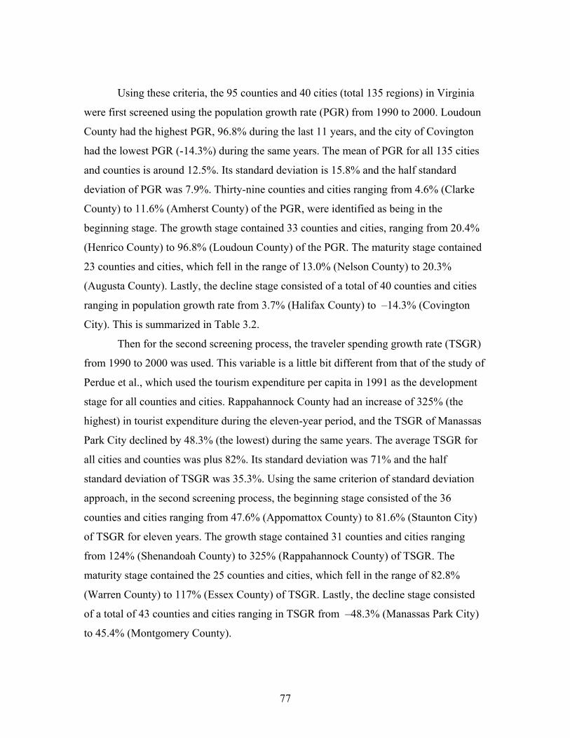
77
Using these criteria, the 95 counties and 40 cities (total 135 regions) in Virginia
were first screened using the population growth rate (PGR) from 1990 to 2000. Loudoun
County had the highest PGR, 96.8% during the last 11 years, and the city of Covington
had the lowest PGR (-14.3%) during the same years. The mean of PGR for all 135 cities
and counties is around 12.5%. Its standard deviation is 15.8% and the half standard
deviation of PGR was 7.9%. Thirty-nine counties and cities ranging from 4.6% (Clarke
County) to 11.6% (Amherst County) of the PGR, were identified as being in the
beginning stage. The growth stage contained 33 counties and cities, ranging from 20.4%
(Henrico County) to 96.8% (Loudoun County) of the PGR. The maturity stage contained
23 counties and cities, which fell in the range of 13.0% (Nelson County) to 20.3%
(Augusta County). Lastly, the decline stage consisted of a total of 40 counties and cities
ranging in population growth rate from 3.7% (Halifax County) to –14.3% (Covington
City). This is summarized in Table 3.2.
Then for the second screening process, the traveler spending growth rate (TSGR)
from 1990 to 2000 was used. This variable is a little bit different from that of the study of
Perdue et al., which used the tourism expenditure per capita in 1991 as the development
stage for all counties and cities. Rappahannock County had an increase of 325% (the
highest) in tourist expenditure during the eleven-year period, and the TSGR of Manassas
Park City declined by 48.3% (the lowest) during the same years. The average TSGR for
all cities and counties was plus 82%. Its standard deviation was 71% and the half
standard deviation of TSGR was 35.3%. Using the same criterion of standard deviation
approach, in the second screening process, the beginning stage consisted of the 36
counties and cities ranging from 47.6% (Appomattox County) to 81.6% (Staunton City)
of TSGR for eleven years. The growth stage contained 31 counties and cities ranging
from 124% (Shenandoah County) to 325% (Rappahannock County) of TSGR. The
maturity stage contained the 25 counties and cities, which fell in the range of 82.8%
(Warren County) to 117% (Essex County) of TSGR. Lastly, the decline stage consisted
of a total of 43 counties and cities ranging in TSGR from –48.3% (Manassas Park City)
to 45.4% (Montgomery County).
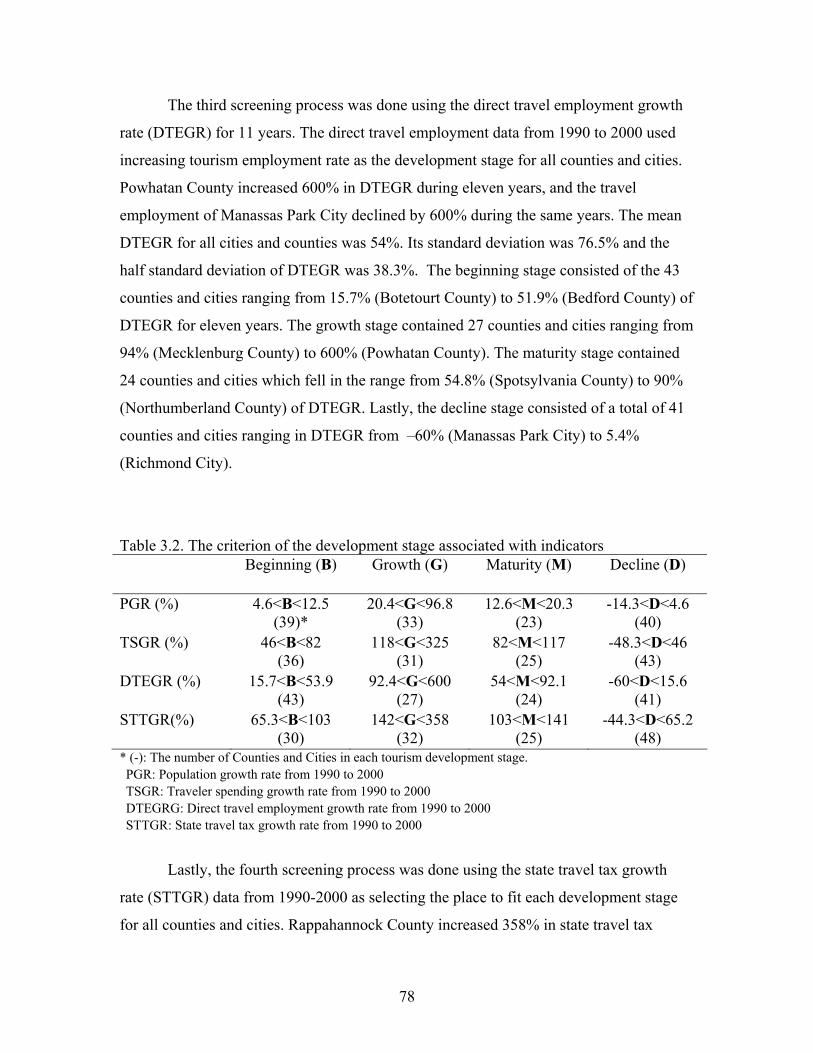
78
The third screening process was done using the direct travel employment growth
rate (DTEGR) for 11 years. The direct travel employment data from 1990 to 2000 used
increasing tourism employment rate as the development stage for all counties and cities.
Powhatan County increased 600% in DTEGR during eleven years, and the travel
employment of Manassas Park City declined by 600% during the same years. The mean
DTEGR for all cities and counties was 54%. Its standard deviation was 76.5% and the
half standard deviation of DTEGR was 38.3%. The beginning stage consisted of the 43
counties and cities ranging from 15.7% (Botetourt County) to 51.9% (Bedford County) of
DTEGR for eleven years. The growth stage contained 27 counties and cities ranging from
94% (Mecklenburg County) to 600% (Powhatan County). The maturity stage contained
24 counties and cities which fell in the range from 54.8% (Spotsylvania County) to 90%
(Northumberland County) of DTEGR. Lastly, the decline stage consisted of a total of 41
counties and cities ranging in DTEGR from –60% (Manassas Park City) to 5.4%
(Richmond City).
Table 3.2. The criterion of the development stage associated with indicators Beginning (B) Growth (G) Maturity (M) Decline (D)
PGR (%)
4.6<B<12.5 (39)*
20.4<G<96.8 (33)
12.6<M<20.3 (23)
-14.3<D<4.6 (40)
TSGR (%)
46<B<82 (36)
118<G<325 (31)
82<M<117 (25)
-48.3<D<46 (43)
DTEGR (%) 15.7<B<53.9 (43)
92.4<G<600 (27)
54<M<92.1 (24)
-60<D<15.6 (41)
STTGR(%) 65.3<B<103 (30)
142<G<358 (32)
103<M<141 (25)
-44.3<D<65.2 (48)
* (-): The number of Counties and Cities in each tourism development stage. PGR: Population growth rate from 1990 to 2000 TSGR: Traveler spending growth rate from 1990 to 2000 DTEGRG: Direct travel employment growth rate from 1990 to 2000 STTGR: State travel tax growth rate from 1990 to 2000
Lastly, the fourth screening process was done using the state travel tax growth
rate (STTGR) data from 1990-2000 as selecting the place to fit each development stage
for all counties and cities. Rappahannock County increased 358% in state travel tax
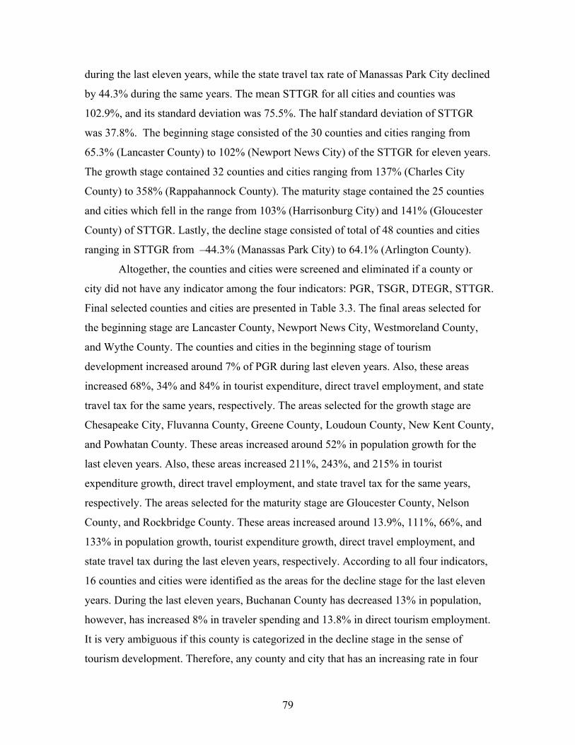
79
during the last eleven years, while the state travel tax rate of Manassas Park City declined
by 44.3% during the same years. The mean STTGR for all cities and counties was
102.9%, and its standard deviation was 75.5%. The half standard deviation of STTGR
was 37.8%. The beginning stage consisted of the 30 counties and cities ranging from
65.3% (Lancaster County) to 102% (Newport News City) of the STTGR for eleven years.
The growth stage contained 32 counties and cities ranging from 137% (Charles City
County) to 358% (Rappahannock County). The maturity stage contained the 25 counties
and cities which fell in the range from 103% (Harrisonburg City) and 141% (Gloucester
County) of STTGR. Lastly, the decline stage consisted of total of 48 counties and cities
ranging in STTGR from –44.3% (Manassas Park City) to 64.1% (Arlington County).
Altogether, the counties and cities were screened and eliminated if a county or
city did not have any indicator among the four indicators: PGR, TSGR, DTEGR, STTGR.
Final selected counties and cities are presented in Table 3.3. The final areas selected for
the beginning stage are Lancaster County, Newport News City, Westmoreland County,
and Wythe County. The counties and cities in the beginning stage of tourism
development increased around 7% of PGR during last eleven years. Also, these areas
increased 68%, 34% and 84% in tourist expenditure, direct travel employment, and state
travel tax for the same years, respectively. The areas selected for the growth stage are
Chesapeake City, Fluvanna County, Greene County, Loudoun County, New Kent County,
and Powhatan County. These areas increased around 52% in population growth for the
last eleven years. Also, these areas increased 211%, 243%, and 215% in tourist
expenditure growth, direct travel employment, and state travel tax for the same years,
respectively. The areas selected for the maturity stage are Gloucester County, Nelson
County, and Rockbridge County. These areas increased around 13.9%, 111%, 66%, and
133% in population growth, tourist expenditure growth, direct travel employment, and
state travel tax during the last eleven years, respectively. According to all four indicators,
16 counties and cities were identified as the areas for the decline stage for the last eleven
years. During the last eleven years, Buchanan County has decreased 13% in population,
however, has increased 8% in traveler spending and 13.8% in direct tourism employment.
It is very ambiguous if this county is categorized in the decline stage in the sense of
tourism development. Therefore, any county and city that has an increasing rate in four

80
indicators in the last eleven years have been excluded. Among 16 counties and cities,
only Covington City and Petersburg City have decreased in terms of population growth,
tourist spending, and direct tourism employment for the last 11 years. These areas have
declined around 11.7% in population growth during last eleven years, 9.9% in tourist
expenditure, and 36.2% in direct travel employment; however, have increased a little bit,
5.6% in state travel tax for the same years.
After all areas for each stage were screened, according to the proportion of the
population in each area, the number of subjects was stratified, and the random sampling
method was then applied. The sample size for each destination is presented in Table 3.3.
Table 3.3. Counties and cities in each stage and the number of stratified sample PGR (%) TSGR(%) DTEGR(%) STTGR(%) POP NOS Beginning Lancaster County 6.2 55.0 21.2 65.34 11567 5% 29 Newport News City 5.1 67.7 31.2 101.99 180150 76% 458 Westmoreland County 8.0 74.6 36.8 84.38 16918 7% 43 Wythe County 8.4 76.3 44.7 82.29 27599 12% 70 ( 6.93) (68.40) (33.48) (83.50) 100% 600 Growth Chesapeake City 31.1 146.7 99.6 177.55 199184 45% 272 Fluvanna County 61.3 270.2 212.5 286.67 20047 5% 27 Greene County 48.0 161.6 177.5 172.50 15244 3% 21 Loudoun County 96.8 231.5 214.3 260.80 169599 39% 231 New Kent County 28.6 192.4 152.7 183.06 13462 3% 18 Powhatan County 46.0 265.0 600.0 270.00 22377 5% 31 (51.97) (211.23) (242.77) (225.10) 100% 600 Maturity Gloucester County 15.4 114.0 55.0 140.96 34780 50% 298 Nelson County 13.0 113.9 76.6 127.45 14445 21% 124 Rockbridge County 13.4 105.2 66.6 129.19 20803 30% 174 (13.93) (111.03) (66.07) (132.53) 100% 600 Decline Covington City -14.3 -13.3 -46.3 7.50 6303 16% 94 Petersburg City -9.0 -6.5 -21.1 3.70 33743 84% 506 (-11.65) (-9.90) (-36.2) (5.60) 100% 600
Note: PGR: Population growth rate from 1990 to 2000, TSGR: Traveler spending growth rate from 1990 to 2000,
DTEGRG: Direct travel employment growth rate from 1990 to 2000, STTGR: State travel tax growth rate from 1990 to 2000, POP: Populations estimated in 2000, NOS: number of stratified samples, (-): mean value
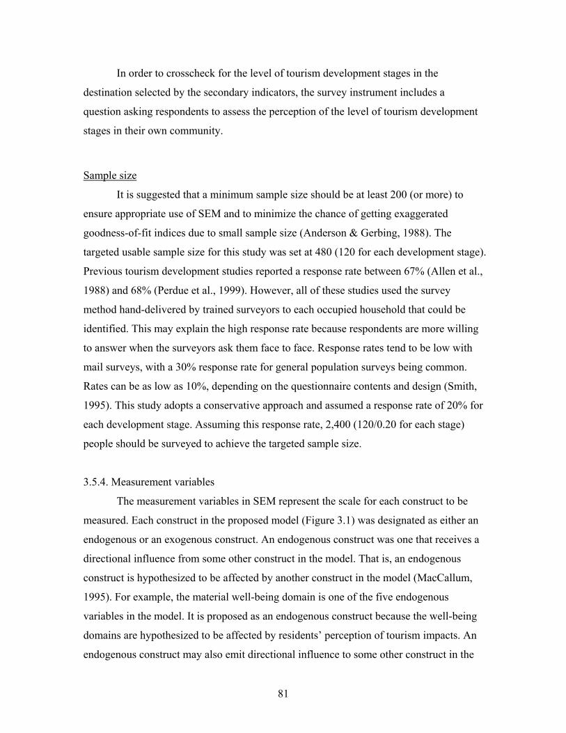
81
In order to crosscheck for the level of tourism development stages in the
destination selected by the secondary indicators, the survey instrument includes a
question asking respondents to assess the perception of the level of tourism development
stages in their own community.
Sample size
It is suggested that a minimum sample size should be at least 200 (or more) to
ensure appropriate use of SEM and to minimize the chance of getting exaggerated
goodness-of-fit indices due to small sample size (Anderson & Gerbing, 1988). The
targeted usable sample size for this study was set at 480 (120 for each development stage).
Previous tourism development studies reported a response rate between 67% (Allen et al.,
1988) and 68% (Perdue et al., 1999). However, all of these studies used the survey
method hand-delivered by trained surveyors to each occupied household that could be
identified. This may explain the high response rate because respondents are more willing
to answer when the surveyors ask them face to face. Response rates tend to be low with
mail surveys, with a 30% response rate for general population surveys being common.
Rates can be as low as 10%, depending on the questionnaire contents and design (Smith,
1995). This study adopts a conservative approach and assumed a response rate of 20% for
each development stage. Assuming this response rate, 2,400 (120/0.20 for each stage)
people should be surveyed to achieve the targeted sample size.
3.5.4. Measurement variables
The measurement variables in SEM represent the scale for each construct to be
measured. Each construct in the proposed model (Figure 3.1) was designated as either an
endogenous or an exogenous construct. An endogenous construct was one that receives a
directional influence from some other construct in the model. That is, an endogenous
construct is hypothesized to be affected by another construct in the model (MacCallum,
1995). For example, the material well-being domain is one of the five endogenous
variables in the model. It is proposed as an endogenous construct because the well-being
domains are hypothesized to be affected by residents’ perception of tourism impacts. An
endogenous construct may also emit directional influence to some other construct in the
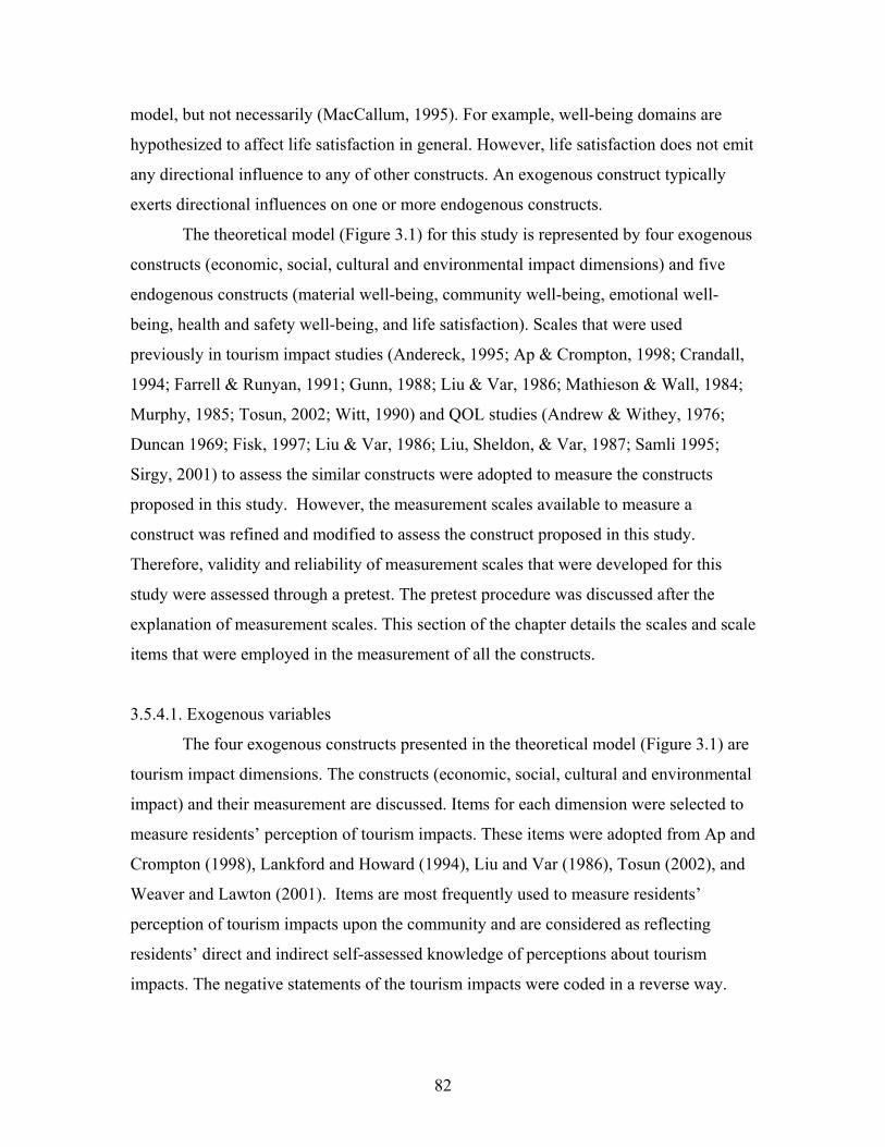
82
model, but not necessarily (MacCallum, 1995). For example, well-being domains are
hypothesized to affect life satisfaction in general. However, life satisfaction does not emit
any directional influence to any of other constructs. An exogenous construct typically
exerts directional influences on one or more endogenous constructs.
The theoretical model (Figure 3.1) for this study is represented by four exogenous
constructs (economic, social, cultural and environmental impact dimensions) and five
endogenous constructs (material well-being, community well-being, emotional well-
being, health and safety well-being, and life satisfaction). Scales that were used
previously in tourism impact studies (Andereck, 1995; Ap & Crompton, 1998; Crandall,
1994; Farrell & Runyan, 1991; Gunn, 1988; Liu & Var, 1986; Mathieson & Wall, 1984;
Murphy, 1985; Tosun, 2002; Witt, 1990) and QOL studies (Andrew & Withey, 1976;
Duncan 1969; Fisk, 1997; Liu & Var, 1986; Liu, Sheldon, & Var, 1987; Samli 1995;
Sirgy, 2001) to assess the similar constructs were adopted to measure the constructs
proposed in this study. However, the measurement scales available to measure a
construct was refined and modified to assess the construct proposed in this study.
Therefore, validity and reliability of measurement scales that were developed for this
study were assessed through a pretest. The pretest procedure was discussed after the
explanation of measurement scales. This section of the chapter details the scales and scale
items that were employed in the measurement of all the constructs.
3.5.4.1. Exogenous variables
The four exogenous constructs presented in the theoretical model (Figure 3.1) are
tourism impact dimensions. The constructs (economic, social, cultural and environmental
impact) and their measurement are discussed. Items for each dimension were selected to
measure residents’ perception of tourism impacts. These items were adopted from Ap and
Crompton (1998), Lankford and Howard (1994), Liu and Var (1986), Tosun (2002), and
Weaver and Lawton (2001). Items are most frequently used to measure residents’
perception of tourism impacts upon the community and are considered as reflecting
residents’ direct and indirect self-assessed knowledge of perceptions about tourism
impacts. The negative statements of the tourism impacts were coded in a reverse way.

83
Economic impact variables
The items to measure (metrics for) economic impacts of tourism can be
categorized into four different sub-dimensions: employment opportunity, revenue from
tourists for local business and government, standard of living, and cost of living. For the
purpose of this study, all four sub-dimensions of economic impacts of tourism were
measured. Items that were used to measure each sub-dimension were summated, and
summated scales were used to assess economic impact of tourism. Three items for
employment opportunity, revenue from tourism for local business, cost of living, and
standard of living were used to measure residents’ perceptions of each economic sub-
dimension. A five-point Likert type (strongly disagree equals one and strongly agree
equals five) was used to measure these items.
Employment opportunity
• Tourism creates employment opportunities for residents in the community.
• Tourism provides highly desirable jobs in the community.
• One of the most important aspects of tourism is that it has created a variety of jobs
for the residents in the community.
Revenue from tourists for local business and government
• Local businesses benefit the most from tourists.
• Tourism brings more investment to the community’s economy.
• Tourism helps national governments generate foreign exchange earnings.
• Tourism generates tax revenues for local governments.
Standard of living
• Our standard of living has increased due to tourist spending in the community.
• Tax revenues from tourism are used to improve roads, highways, and public
services for residents.
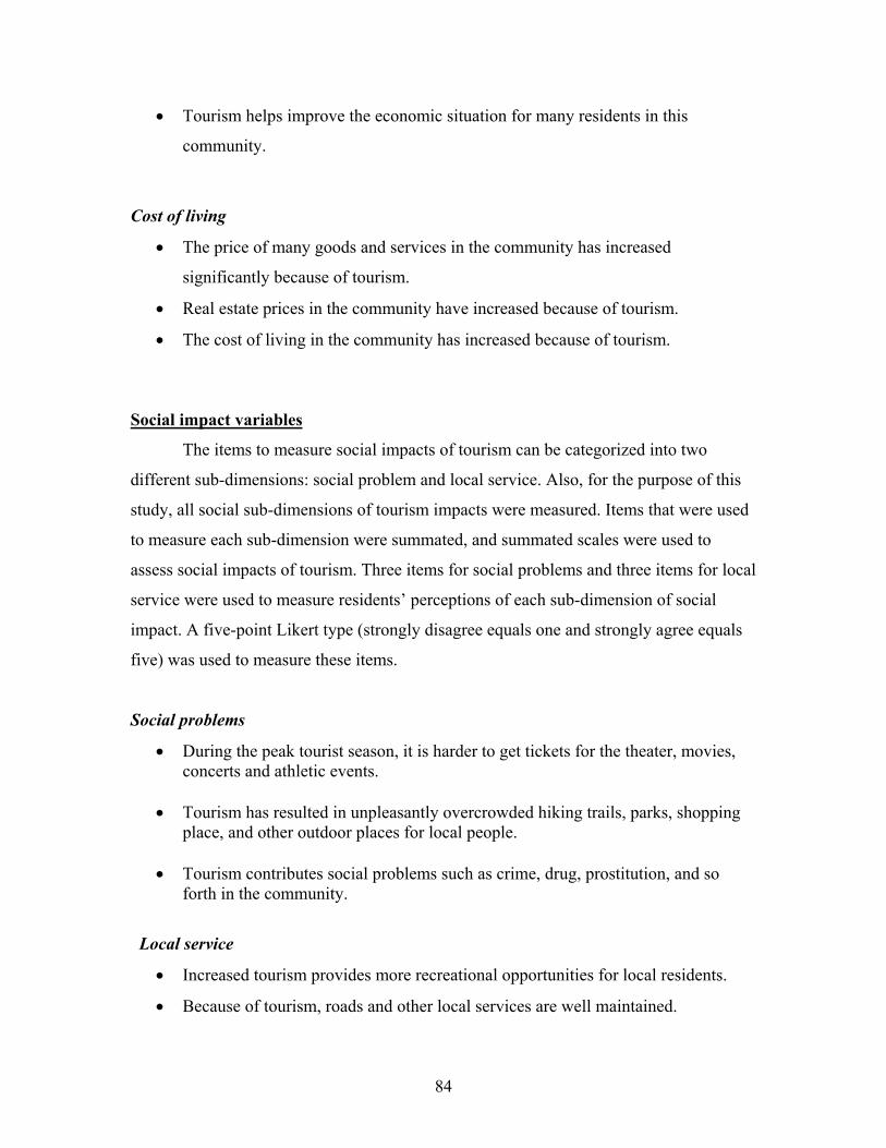
84
• Tourism helps improve the economic situation for many residents in this
community.
Cost of living
• The price of many goods and services in the community has increased
significantly because of tourism.
• Real estate prices in the community have increased because of tourism.
• The cost of living in the community has increased because of tourism.
Social impact variables
The items to measure social impacts of tourism can be categorized into two
different sub-dimensions: social problem and local service. Also, for the purpose of this
study, all social sub-dimensions of tourism impacts were measured. Items that were used
to measure each sub-dimension were summated, and summated scales were used to
assess social impacts of tourism. Three items for social problems and three items for local
service were used to measure residents’ perceptions of each sub-dimension of social
impact. A five-point Likert type (strongly disagree equals one and strongly agree equals
five) was used to measure these items.
Social problems
• During the peak tourist season, it is harder to get tickets for the theater, movies, concerts and athletic events.
• Tourism has resulted in unpleasantly overcrowded hiking trails, parks, shopping
place, and other outdoor places for local people.
• Tourism contributes social problems such as crime, drug, prostitution, and so forth in the community.
Local service
• Increased tourism provides more recreational opportunities for local residents.
• Because of tourism, roads and other local services are well maintained.

85
• Tourism is a major reason for the variety of entertainment in the community.
Cultural impact variables
The items to measure cultural impacts of tourism can be categorized into three
different sub-dimensions: preservation of the local culture, deterioration of the local
culture, and cultural exchange between residents and tourists. Three cultural sub-
dimensions of tourism impacts were measured. Items that were used to measure each sub-
dimension were summated, and summated scales were used to assess cultural impact of
tourism. Three items for preservation of local culture, three items for deterioration of the
local culture, and three items for cultural exchange between residents and tourists were
used to measure residents’ perceptions of each sub-dimension of cultural impact. A five-
point Likert scale (strongly disagree equals one and strongly agree equals five) was used
to measure these items.
Preservation of local culture
• Tourism has increased residents’ pride in the local culture in the community.
• Tourism helps keep local culture alive and maintain cultural identity.
• Tourism encourages a variety of cultural activities for local residents.
Deterioration of local culture
• The commercial demand of tourists causes change in the style and forms of traditional arts and crafts.
• Tourism encourages residents to imitate the behavior of the tourists and relinquish
cultural traditions.
• Tourism causes the disruption of traditional cultural behavior patterns in local residents.
Cultural exchange between residents and tourists
• Meeting tourists from all over the world is definitely a life enriching experience.
• The cultural exchange between residents and tourists is valuable and pleasant for
the residents.
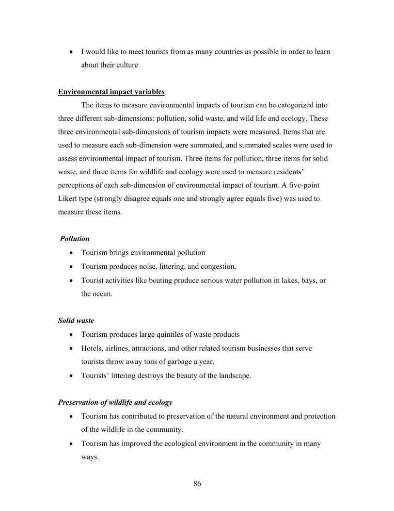
86
• I would like to meet tourists from as many countries as possible in order to learn
about their culture
Environmental impact variables
The items to measure environmental impacts of tourism can be categorized into
three different sub-dimensions: pollution, solid waste, and wild life and ecology. These
three environmental sub-dimensions of tourism impacts were measured. Items that are
used to measure each sub-dimension were summated, and summated scales were used to
assess environmental impact of tourism. Three items for pollution, three items for solid
waste, and three items for wildlife and ecology were used to measure residents’
perceptions of each sub-dimension of environmental impact of tourism. A five-point
Likert type (strongly disagree equals one and strongly agree equals five) was used to
measure these items.
Pollution
• Tourism brings environmental pollution
• Tourism produces noise, littering, and congestion.
• Tourist activities like boating produce serious water pollution in lakes, bays, or
the ocean.
Solid waste
• Tourism produces large quintiles of waste products
• Hotels, airlines, attractions, and other related tourism businesses that serve
tourists throw away tons of garbage a year.
• Tourists’ littering destroys the beauty of the landscape.
Preservation of wildlife and ecology
• Tourism has contributed to preservation of the natural environment and protection
of the wildlife in the community.
• Tourism has improved the ecological environment in the community in many
ways.

87
• Tourism does not contribute to the negative effect of vegetation and loss of
meadows and green space.
3.5.4.2. Endogenous variables
Five endogenous constructs that are presented in the theoretical model (Figure
3.1) are material well-being, community well-being, emotional well-being, health and
safety well-being, other well-being (these are used as covariate variables) and life
satisfaction in general. The items were adopted from Andrew and Withey (1976),
Cicerchia (1996), Cummins (1996), and Sirgy (2001). In the next section, these five
constructs and the measurement items used to assess these constructs are discussed.
Material well-being variables
The satisfaction of material well-being can be shared in the form of cost of living
and income and employment. These two material sub-domains were measured. Items that
were used to measure each sub-dimension were summated, and summated scales were
used to assess material well-being domains. Three items for cost of living and four items
for income and employment were used to measure residents’ satisfaction of material
well-being. The items were adopted from Andrew and Withey (1976), Cicerchia (1996),
Cummins (1996) and Sirgy (2001). These items were measured on a five-point Likert-
type with classifications of very dissatisfied, dissatisfied, mixed feeling, satisfied, very
satisfied.
Cost of living
• How satisfied are you with real estate taxes?
• How satisfied are you with the cost of living in your community?
• How satisfied are you with the cost of basic necessities such as food, housing and
clothing?
Income and employment
• How satisfied are your income at your current job?

88
• How satisfied are you with the economic security of your job?
• How satisfied are you with your family income?
• How satisfied are you with the pay and fringe benefits you get?
Community well-being variable
There are many aspects of community life and setting that make up people’s
appreciation or dissatisfaction with the greater than neighborhood area where they live.
Four items were used to measure the community well-being domain. The items came
from the studies of Andrew and Withey (1978), Cummins (1996), Norman et al. (1997),
and O’Brian and Lange (1986). These items were also measured on a five-point Likert-
type scale with classifications of very dissatisfied, dissatisfied, mixed feeling, satisfied,
very satisfied.
• How satisfied are you with the conditions of the community environment (air,
water, land)?
• How satisfied are you with the people who live in this community?
• How satisfied are you with the service and facilities you get in this community?
• How satisfied are you with your community life?
Emotional well-being variables
Emotional well-being can be satisfied in the form of leisure well-being and
spiritual well-being (Cummins, 1997). These two emotional well-being sub-domains
were measured. Items that were used to measure each sub-dimension were summated,
and summated scales were used to assess emotional well-being domains. Four items for
leisure well-being and five items for spiritual well-being were proposed to measure
residents’ satisfaction of the emotional well-being. The items were adopted from Andrew
and Withey (1976), Cicerchia (1996), Cummins (1996), Neal et al. (1995, 1999), Norman
et al. (1997) and Sirgy (2001). The items for leisure activity were measured on a five-
point Likert-type scale with classifications of very dissatisfied, dissatisfied, mixed feeling,
satisfied, very satisfied. The items for spiritual activity were measured on a five-point
Likert-type scale with strongly disagree, disagree neutral, agree, and strongly agree.

89
Leisure activity
• How satisfied are you with spare time?
• How satisfied are you with your leisure activity in your community?
• How satisfied are you with the influx of tourists from all over the world you’re
your community?
• How satisfied are you with leisure life?
Spiritual activity
• I am very satisfied with the availabilities of religious services in my community?
• I am particularly happy with the way we preserve culture in my community.
• I feel I extend my cultural outlook when I talk with tourists.
• I am very satisfied with the leisure life in the community.
• I am very satisfied with the spiritual life in the community.
Health and Safety well-being variables
The satisfaction of health and safety well-being consists of health well-being and
safety well-being. These two well-being domains were measured. Items that were used to
measure each domain were summated, and summated scales were used to assess the
health and safety well-being domain.
Health well-being
Six items for health well-being were proposed to measure satisfaction of health
well-being domain. Three items were measured on a five-point Likert-type scale with
classifications of very dissatisfied, dissatisfied, mixed feeling, satisfied, very satisfied.
• How satisfied are you with your health?
• How satisfied are you with water quality in your area?
• How satisfied are you with air quality in your area?
Three items were measured on a five-point Likert-type scale with classifications of
strongly disagree, disagree, neutral, agree, and strongly agree.
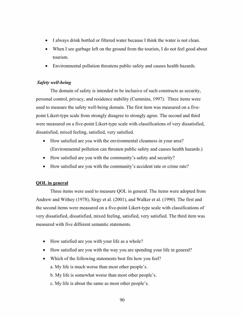
90
• I always drink bottled or filtered water because I think the water is not clean.
• When I see garbage left on the ground from the tourists, I do not feel good about
tourism.
• Environmental pollution threatens public safety and causes health hazards.
Safety well-being
The domain of safety is intended to be inclusive of such constructs as security,
personal control, privacy, and residence stability (Cummins, 1997). Three items were
used to measure the safety well-being domain. The first item was measured on a five-
point Likert-type scale from strongly disagree to strongly agree. The second and third
were measured on a five-point Likert-type scale with classifications of very dissatisfied,
dissatisfied, mixed feeling, satisfied, very satisfied.
• How satisfied are you with the environmental cleanness in your area?
(Environmental pollution can threaten public safety and causes health hazards.)
• How satisfied are you with the community’s safety and security?
• How satisfied are you with the community’s accident rate or crime rate?
QOL in general
Three items were used to measure QOL in general. The items were adopted from
Andrew and Withey (1978), Sirgy et al. (2001), and Walker et al. (1990). The first and
the second items were measured on a five-point Likert-type scale with classifications of
very dissatisfied, dissatisfied, mixed feeling, satisfied, very satisfied. The third item was
measured with five different semantic statements.
• How satisfied are you with your life as a whole?
• How satisfied are you with the way you are spending your life in general?
• Which of the following statements best fits how you feel?
a. My life is much worse than most other people’s.
b. My life is somewhat worse than most other people’s.
c. My life is about the same as most other people’s.

91
d. My life is somewhat better than most other people’s.
e. My life is much better than most other people’s.
3.5.5 Pretest of the measurement instrument
Since some of the measurement items were developed and modified for the
purpose of this study, pretest of the measurement instrument was necessary to validate
the items in the scales. A pretest of the measurement instrument was conducted in several
stages. First, the survey questionnaire was circulated to several faculty and graduate
students in the Department of Hospitality and Tourism Management at Virginia
Polytechnic Institute and State University. Participants were asked to provide feedback
regarding the layout, wording, and ease of understanding of the measurement items. The
feedback was then taken into account in the revision of the questionnaire. The revised
questionnaire was pre-tested using a convenience sample of undergraduate and graduate
students, faculty, and residents of Blacksburg, Virginia. The responses from the pretest
were analyzed to test reliability and validity of the measurement items. The questionnaire
was revised based on the reliability and validity tests and the final version of the
questionnaire was developed. The final questionnaire was produced in a booklet form.
3.6 RELIABILITY AND VALIDITY
Reliability deals with how consistently similar measures produce similar results
(Rosenthal & Rosnow, 1984). Reliability has two dimensions: repeatability and internal
consistency (Zigmund, 1995). The dimension of internal consistency refers to the ability
of a scale item to correlate with other items of the sample scale that are intended to
measure the same construct. The adequacy of the individual items and the composites
were assessed by measures of reliability and validity. The reliability of the measurement
instrument was assessed by Cronbach’s alpha. A Cronbach’s alpha and composite
reliability estimate of 0.70 or higher indicate that the measurement scale that is used to
measure a construct is moderately reliable. If the composite reliability was not high
enough to be accepted, the scales were revised by deleting items as a result of the
92
reliability analysis. The composite reliability, as calculated with LISREL estimates, is
analogous to coefficient alpha and was calculated by the formula by Fornell and Larcker
(1981).
Validity refers to how well the measurement captures what it is designed to
measure (Rosenthal & Rosnow, 1984). There are several different types of validity about
which to be concerned: face/content validity (i.e., the agreement among professionals that
the scale is measuring what it is supposed to measure), criterion validity (e.g., the degree
of correspondence between a measure and a criterion variable, usually measured by their
correlation), and construct validity (i.e., the ability of a measure to confirm a network of
related hypotheses generated from a theory based on constructs) (Bollen, 1989; Zigmund,
1995).
Face validity of the measurement instrument was assessed by allowing four
professionals to examine it and provide feedback for revision. Afterwards, the survey
instrument was given to fourteen graduate students majoring in hospitality and tourism
management to solicit feedback as well as to check for readability of the questions and
estimated time to complete the survey questionnaire. Additionally, a formal pretest was
conducted on a convenience sample.
Convergent validity was assessed from the measurement model by deleting each
indicator’s estimated pattern coefficient on its posited underlying construct factor and
determining if a chi-square difference test between a model with and without the
estimated parameter is significant (greater than twice its standard error, Anderson &
Gerbing, 1988).
Discriminant validity was assessed for every possible pair of constructs by
constraining the estimated correlation parameter between them to 1.0 and then
performing a chi-square difference test on the values obtained for the constrained and
unconstrained model (Anderson & Gerbing, 1988). A significantly lower chi-square
value for the model in which the trait correlations are not constrained to unity indicates
that the traits are not perfectly correlated and that discriminant validity is achieved.

93
3.7 CHAPTER SUMMARY
This chapter outlines the research design for the study. It includes the description
of the survey population, the method of the data collection, and the statistical methods
that were employed to analyze the data. Special attention was given to the selecting
procedure of the tourism destination area to fit each tourism development stage. The
results of data gathering and its analysis are presented in the next section.
94
CHAPTER IV
ANALYSIS AND RESULTS
4.1 INTRODUCTION
This chapter presents the results of the data analysis and hypothesis testing. In the
first section of this chapter, the pretest of the scale items used in the study is presented,
including a description of the samples. This is followed by a section that provides a
description of the survey methods employed in this study and the demographic profiles of
the survey respondents. The third section of the chapter presents the results of the
confirmatory factor analysis conducted to confirm the factor structure of the nine
constructs. The fourth section of the chapter presents a discussion of the data analysis
steps. This is followed by a section that presents a discussion of the procedures for the
validity checks in detail and the results of the hypothesis testing.
4.2 PRETEST
As stated in Chapter III, before the final survey instrument could be prepared, it
was necessary to conduct a pretest of scale items. The purpose of the pretest was to
validate the scale items to be used in the study that were either developed specifically for
this study or modified from previous studies.
The development of the measurement scales for this study followed the
procedures recommended by Churchill (1979) and DeVellis (1991) for developing a
standardized survey instrument. The initial task in developing a scale is to devise an item
pool (Lankford & Howard 1994; Liu, Sheldon, & Var, 1987). A total of 37 items were
used to measure tourism impacts (thirteen items to measure economic impacts: six items
to measure social impacts; nine items for cultural impacts; and nine items to assess
environmental impacts), and 30 items for assessing residents’ satisfaction with various
95
life domains (nine items for material life domains; four items for the community life
domain; eight items for the emotional life domain; and nine items to measure the health
and safety life domain); three items were used to measure residents’ overall life
satisfaction.
Four professors first assessed the content adequacy of the items. The professors
were asked to provide comments on content and understandability. They were then asked
to edit and improve the items to enhance their clarity, readability, and content adequacy.
They were also asked to identify any of the scale items that were redundant with other
scale items, and to offer suggestions for improving the proposed scale. Afterwards, the
measurement items were distributed to 14 graduate students. They were also asked to
comment on content and provide additional questions that might improve the scale and
understandability, and asked to identify any of the scale items that were redundant with
other scale items. Three professors commented that the questionnaire had confounded
problems. To remove the confound problems, two additional questions were added to the
measurement scale that measures the social impacts of tourism, another item was added
to the items that measure the cultural impact of tourism, two other items were added that
measure the environmental impacts of tourism, and one more item was added to the items
that measure community well-being. Thus, the total number of items was increased to 76.
Then, the newly developed and modified scale items that had been drawn from previous
studies were tested empirically. This step in the pretest is discussed in detail in this
section of the chapter.
4.2.1. Pretest Survey method
The pretest survey was distributed by several methods. One method was to send it
as an e-mail attachment in Word 2000 format. This method allowed the respondent to
take the survey on his or her computer, save the file in Microsoft Word format and then
send it back to a designated email-address as an attachment. The respondent could also
print out the survey, take it by hand and fax it back to a specified fax number or mail it to
a specified mailing address. Another method used was to distribute the printed
questionnaires in a classroom and in an apartment complex. This method allowed
respondents to complete the survey and drop it in a designated mailbox.
96
4.2.2. Pretest sample
A convenient sample was used to conduct the pretest. The sample consisted of
faculty, graduate students, and undergraduate students of Virginia Tech, and residents in
Blacksburg, Virginia. A total of 133 responses was received from the various places and
methods: 14 responses from the apartment complex, 34 from the classroom, 20 handed
in, 1 by mail, and 64 responses through email. The final pretest sample size was 133.
Table 4.1 presents the demographics of the pretest sample.
The demographics of the sample indicate that 59.5 percent of the respondents
were male and 40.5 percent were female (Table 4.1). Average age of the respondents was
29.84. The youngest respondent was 19 years old; the oldest was 81 years of age. The
standard deviation of the age was 15 years old. A majority of respondents (55%) were
Caucasian; 46.8% of respondents had a masters degree. The majority of respondents
(52.5%) had a household income of less than $20,000.
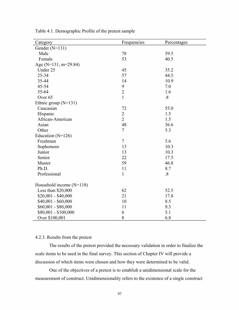
97
Table 4.1. Demographic Profile of the pretest sample Category Frequencies Percentages Gender (N=131) Male Female
78 53
59.5 40.5
Age (N=131, m=29.84) Under 25 25-34 35-44 45-54 55-64 Over 65
45 57 14 9 2 1
35.2 44.5 10.9 7.0 1.6 .8
Ethnic group (N=131) Caucasian Hispanic African-American Asian Other
72 2 2 48 7
55.0 1.5 1.5 36.6 5.3
Education (N=126) Freshman Sophomore Junior Senior Master Ph.D. Professional
7 13 13 22 59 11 1
5.6 10.3 10.3 17.5 46.8 8.7 .8
Household income (N=118) Less than $20,000 $20,001 - $40,000 $40,001 - $60,000 $60,001 - $80,000 $80,001 - $100,000 Over $100,001
62 21 10 11 6 8
52.5 17.8 8.5 9.3 5.1 6.8
4.2.3. Results from the pretest
The results of the pretest provided the necessary validation in order to finalize the
scale items to be used in the final survey. This section of Chapter IV will provide a
discussion of which items were chosen and how they were determined to be valid.
One of the objectives of a pretest is to establish a unidimensional scale for the
measurement of construct. Unidimensionality refers to the existence of a single construct
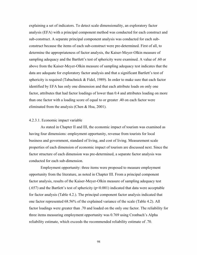
98
explaining a set of indicators. To detect scale dimensionality, an exploratory factor
analysis (EFA) with a principal component method was conducted for each construct and
sub-construct. A separate principal component analysis was conducted for each sub-
construct because the items of each sub-construct were pre-determined. First of all, to
determine the appropriateness of factor analysis, the Kaiser-Meyer-Olkin measure of
sampling adequacy and the Bartlett’s test of sphericity were examined. A value of .60 or
above from the Kaiser-Meyer-Olkin measure of sampling adequacy test indicates that the
data are adequate for exploratory factor analysis and that a significant Bartlett’s test of
sphericity is required (Tabachnick & Fidel, 1989). In order to make sure that each factor
identified by EFA has only one dimension and that each attribute loads on only one
factor, attributes that had factor loadings of lower than 0.4 and attributes loading on more
than one factor with a loading score of equal to or greater .40 on each factor were
eliminated from the analysis (Chen & Hsu, 2001).
4.2.3.1. Economic impact variable
As stated in Chapter II and III, the economic impact of tourism was examined as
having four dimensions: employment opportunity, revenue from tourists for local
business and government, standard of living, and cost of living. Measurement scale
properties of each dimension of economic impact of tourism are discussed next. Since the
factor structure of each dimension was pre-determined, a separate factor analysis was
conducted for each sub-dimension.
Employment opportunity: three items were proposed to measure employment
opportunity from the literature, as noted in Chapter III. From a principal component
factor analysis, results of the Kaiser-Meyer-Olkin measure of sampling adequacy test
(.657) and the Bartlett’s test of sphericity (p<0.001) indicated that data were acceptable
for factor analysis (Table 4.2.). The principal component factor analysis indicated that
one factor represented 68.56% of the explained variance of the scale (Table 4.2). All
factor loadings were greater than .70 and loaded on the only one factor. The reliability for
three items measuring employment opportunity was 0.769 using Cronbach’s Alpha
reliability estimate, which exceeds the recommended reliability estimate of .70.

99
Therefore, it was concluded that the employment opportunity sub-construct could be
measured by three items.
Revenue from tourists for local business and government: four items were
proposed to measure revenue from tourists for local business and government from
literature as noted in Chapter III. From a principal component factor analysis, results of
the Kaiser-Meyer-Olkin measure of sampling adequacy test (.664) and the Bartlett’s test
of sphericity (p<0.001) indicated that data were acceptable for factor analysis (Table
4.2.). The principal component analysis indicated that one factor explained 57.7%
variance of explained, and all four items loaded on greater than .70. The Cronbach’s
reliability estimate indicated that the reliability score was 0.74.
Standard of living: three items were proposed to measure standard of living from
literature as noted in Chapter III. From a principal component factor analysis, results of
the Kaiser-Meyer-Olkin measure of sampling adequacy test (.680) and the Bartlett’s test
of sphericity (p<0.001) indicated that data were acceptable for factor analysis (Table
4.2.). All factor loadings were greater than .70 and loaded on only one factor. The
reliability estimate was 0.72; three items explained 64% of the variance of standard of
living.
Cost of living: three items were proposed to measure the cost of living from
literature as noted in Chapter III. From a principal component factor analysis, results of
the Kaiser-Meyer-Olkin measure of sampling adequacy test (.722) and the Bartlett’s test
of sphericity (p<0.001) indicated that data were acceptable for factor analysis (Table
4.2.). All factor loadings were greater than .70 and loaded on only one factor. The
reliability of the three items meaning cost of living was 0.87 and the variance explained
was 80%.
Table 4.2 clearly showed that the Cronbach’s reliability estimate for all four sub-
dimensions of the economic impacts of the tourism was greater than .70 and exceeded the
requirement of acceptable level. Also, the variance explained for all four sub-dimensions
of the economic impacts of tourism was above .50, indicating that variance due to
measurement error is smaller than the variance captured by the factor. Therefore, it was
concluded that employment opportunity can be measured by three items, revenue from
tourist for local business and government can be measured by four items, standard of
100
living can be measured by three items, and cost of living can be measured by three items.
It was also concluded that all items are valid and reliable.
Table 4.2. Factor analysis result of the economic impact of tourism construct
Constructs and scales Loading Eigenvalues
Variance Explained
Employment opportunity Provides desirable jobs Creates variety of jobs Creates employment opportunity Kaiser-Meyer-Olkin MSA Bartlett's Test of Sphericity Revenue from tourist for local business and government Brings more investment and spending Local government generates foreign exchange Generates tax revenues for local governments Local business benefits from tourism Kaiser-Meyer-Olkin MSA Bartlett's Test of Sphericity Standard of living Standard of living increases Improve economic situation To improve roads, highways, and public services Kaiser-Meyer-Olkin MSA Bartlett's Test of Sphericity Cost of living The cost of living in the community The price of goods and service increases Real estate prices in the community Kaiser-Meyer-Olkin MSA Bartlett's Test of Sphericity
.77*
.881
.838
.760 .657 .000 .74* .861 .752 .715 .701 .664 .000 .72* .808 .806 .788 .680 .000 .87* .920 .883 .874 .722 .000
2.057 2.308 1.923 2.389
68.56% 57.71% 64.10% 79.65%
Note: A separate factor analysis was conducted for each sub-dimension but reported in a table. * Reliability coefficient (Cronbach’s Alpha)
101
4.2.3.2. Social impact variables
As stated in Chapters II and III, the social impact of tourism was examined as
having two dimensions: social problem and local service. Measurement scale properties
of each dimension of social impact of tourism are discussed next. Since the factor
structure of each dimension was pre-determined, a separate factor analysis was conducted
for each sub-dimension.
Social problem: three items were proposed to measure social problem from
literature as noted in Chapter III. The items were: “during peak tourist season, I find it
harder to get tickets for the theater, movies, concerts, or athletic events”; “Tourism has
resulted in unpleasantly overcrowded hiking trails, parks, shopping places, or other
outdoor facilities for local residents”; and “tourism increases social problems such as
crime, drug, prostitution and so forth in the community.” From a principal component
factor analysis, results of the Kaiser-Meyer-Olkin measure of sampling adequacy test
(.634) and the Bartlett’s test of sphericity (p<0.001) indicated that data were acceptable
for factor analysis (Table 4.3.). The principal component analysis indicated that there was
only one factor and represented 62% of the explained variance of the scale. The factor
was composed of three items with factor loadings greater than 0.70. Cronbach’s alpha
reliability was 0.69, which is below the guideline established in Chapter III. However, it
was determined to keep this factor because reliability estimates between 0.6 and 0.7
represent the lower limit of acceptability (Hair et al., 1998). However, the second item
was divided into three items in response to an expert’s advice that the item might have a
possibility to evoke confounding error.
Local service: three items were proposed to measure local service from literature,
as noted in Chapter III. From a principal component factor analysis, results of the Kaiser-
Meyer-Olkin measure of sampling adequacy test (.644) and the Bartlett’s test of
sphericity (p<0.001) indicated that data were acceptable for factor analysis (Table 4.3).
All factor loadings were greater than .70 and loaded on only one factor with the
explained 63% of variance. The reliability of three items measuring the local service was
0.71 using Cronbach’s alpha, which exceeds the recommended reliability estimate of
0.70.
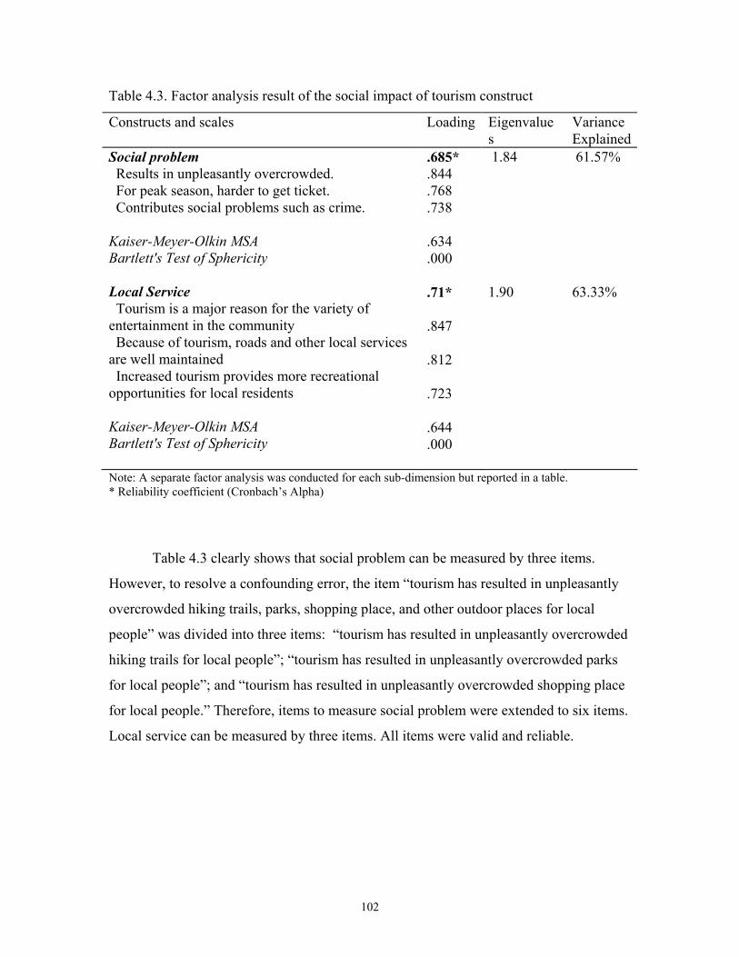
102
Table 4.3. Factor analysis result of the social impact of tourism construct
Constructs and scales Loading Eigenvalues
Variance Explained
Social problem Results in unpleasantly overcrowded. For peak season, harder to get ticket. Contributes social problems such as crime. Kaiser-Meyer-Olkin MSA Bartlett's Test of Sphericity Local Service Tourism is a major reason for the variety of entertainment in the community Because of tourism, roads and other local services are well maintained Increased tourism provides more recreational opportunities for local residents Kaiser-Meyer-Olkin MSA Bartlett's Test of Sphericity
.685*
.844
.768
.738 .634 .000 .71* .847 .812 .723 .644 .000
1.84 1.90
61.57% 63.33%
Note: A separate factor analysis was conducted for each sub-dimension but reported in a table. * Reliability coefficient (Cronbach’s Alpha)
Table 4.3 clearly shows that social problem can be measured by three items.
However, to resolve a confounding error, the item “tourism has resulted in unpleasantly
overcrowded hiking trails, parks, shopping place, and other outdoor places for local
people” was divided into three items: “tourism has resulted in unpleasantly overcrowded
hiking trails for local people”; “tourism has resulted in unpleasantly overcrowded parks
for local people”; and “tourism has resulted in unpleasantly overcrowded shopping place
for local people.” Therefore, items to measure social problem were extended to six items.
Local service can be measured by three items. All items were valid and reliable.
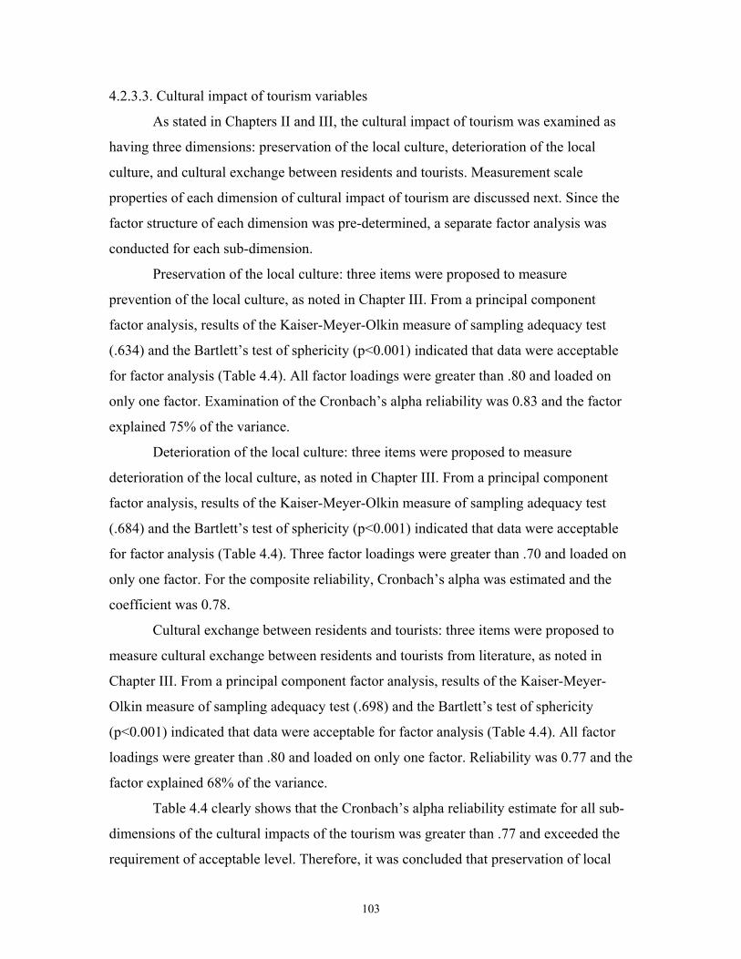
103
4.2.3.3. Cultural impact of tourism variables
As stated in Chapters II and III, the cultural impact of tourism was examined as
having three dimensions: preservation of the local culture, deterioration of the local
culture, and cultural exchange between residents and tourists. Measurement scale
properties of each dimension of cultural impact of tourism are discussed next. Since the
factor structure of each dimension was pre-determined, a separate factor analysis was
conducted for each sub-dimension.
Preservation of the local culture: three items were proposed to measure
prevention of the local culture, as noted in Chapter III. From a principal component
factor analysis, results of the Kaiser-Meyer-Olkin measure of sampling adequacy test
(.634) and the Bartlett’s test of sphericity (p<0.001) indicated that data were acceptable
for factor analysis (Table 4.4). All factor loadings were greater than .80 and loaded on
only one factor. Examination of the Cronbach’s alpha reliability was 0.83 and the factor
explained 75% of the variance.
Deterioration of the local culture: three items were proposed to measure
deterioration of the local culture, as noted in Chapter III. From a principal component
factor analysis, results of the Kaiser-Meyer-Olkin measure of sampling adequacy test
(.684) and the Bartlett’s test of sphericity (p<0.001) indicated that data were acceptable
for factor analysis (Table 4.4). Three factor loadings were greater than .70 and loaded on
only one factor. For the composite reliability, Cronbach’s alpha was estimated and the
coefficient was 0.78.
Cultural exchange between residents and tourists: three items were proposed to
measure cultural exchange between residents and tourists from literature, as noted in
Chapter III. From a principal component factor analysis, results of the Kaiser-Meyer-
Olkin measure of sampling adequacy test (.698) and the Bartlett’s test of sphericity
(p<0.001) indicated that data were acceptable for factor analysis (Table 4.4). All factor
loadings were greater than .80 and loaded on only one factor. Reliability was 0.77 and the
factor explained 68% of the variance.
Table 4.4 clearly shows that the Cronbach’s alpha reliability estimate for all sub-
dimensions of the cultural impacts of the tourism was greater than .77 and exceeded the
requirement of acceptable level. Therefore, it was concluded that preservation of local
104
culture can be measured by three items, deterioration of local service can be measured by
three items, and the cultural exchange dimension can be measured by three items. All
items were deemed valid and reliable.
Table 4.4. Factor analysis result of the cultural impact of tourism construct
Constructs and scales Loading Eigenvalues
Variance Explained
Preservation of local service Tourism encourages a variety of cultural activities for local residents. Tourism helps keep local culture alive and maintain cultural identity. Tourism has increased residents’ pride in the local culture in the community Kaiser-Meyer-Olkin MSA Bartlett's Test of Sphericity Deterioration of local service Tourism encourages residents to imitate the behavior of the tourists and relinquish cultural traditions. The commercial demand of tourists causes change in the style and forms of traditional arts and crafts. Tourism causes the disruption of traditional cultural behavior patterns in local residents. Kaiser-Meyer-Olkin MSA Bartlett's Test of Sphericity Cultural exchange Meeting tourists from all over the world is definitely a life-enriching experience. I would like to meet tourists from as many countries as possible in order to learn about their culture. The cultural exchange between residents and tourists is valuable and pleasant for the residents. Kaiser-Meyer-Olkin MSA Bartlett's Test of Sphericity
.83* .894 .859 .838 .707 .000 .78* .868 .843 .788 .684 .000 .77* .835 .829 .814 .698 .000
2.239 2.086 2.049
74.64% 69.55% 68.29%
Note: A separate factor analysis was conducted for each sub-dimension but reported in a table. * Reliability coefficient (Cronbach’s Alpha)
105
4.2.3.4. Environmental impact of tourism variables
As stated in Chapters II and III, the environmental impact of tourism was
examined as having three dimensions: pollution, solid waste, and preservation wild life
and ecology. Measurement scale properties of each dimension of environmental impact
of tourism are discussed next. Since the factor structure of each dimension was pre-
determined, a separate factor analysis was conducted for each sub-dimension.
Pollution: three items were proposed to measure pollution from literature, as
noted in Chapter III. From a principal component factor analysis, results of the Kaiser-
Meyer-Olkin measure of sampling adequacy test (.707) and the Bartlett’s test of
sphericity (p<0.001) indicated that data were acceptable for factor analysis (Table 4.5).
All factor loadings were greater than .80 and loaded on only one factor. The factor
reliability estimate was 0.89 and the factor represented 81% of the variance.
Solid waste: three items were proposed to measure deterioration of solid waste of
environmental impacts of tourism from literature, as noted in Chapter III. From a
principal component factor analysis, results of the Kaiser-Meyer-Olkin measure of
sampling adequacy test (.704) and the Bartlett’s test of sphericity (p<0.001) indicated
that data were acceptable for factor analysis (Table 4.5). Three factor loadings were
greater than .80 and loaded on only one factor. Cronbach alpha’s reliability was 0.82 and
the factor explained 74% of the variance.
Preservation of wild life and ecology: three items were proposed to measure
preservation of wild life and ecology from the literature, as noted in Chapter III. From a
principal component factor analysis, results of the Kaiser-Meyer-Olkin measure of
sampling adequacy test (.568) and the Bartlett’s test of sphericity (p<0.001) indicated
that data were acceptable for factor analysis (Table 4.5). Even though the loading value
(.558) of the item “tourism does not contribute to the negative effect of vegetation and
loss of meadows and green space” was not high compared to other two items (two other
loadings were greater than .80), it was still over .40, and all three items loaded on only
one factor. Therefore, all three items were kept to measure preservation of wild life and
ecology. Cronbach alpha reliability was 0.70 and the factor represented 64% of the
variance.
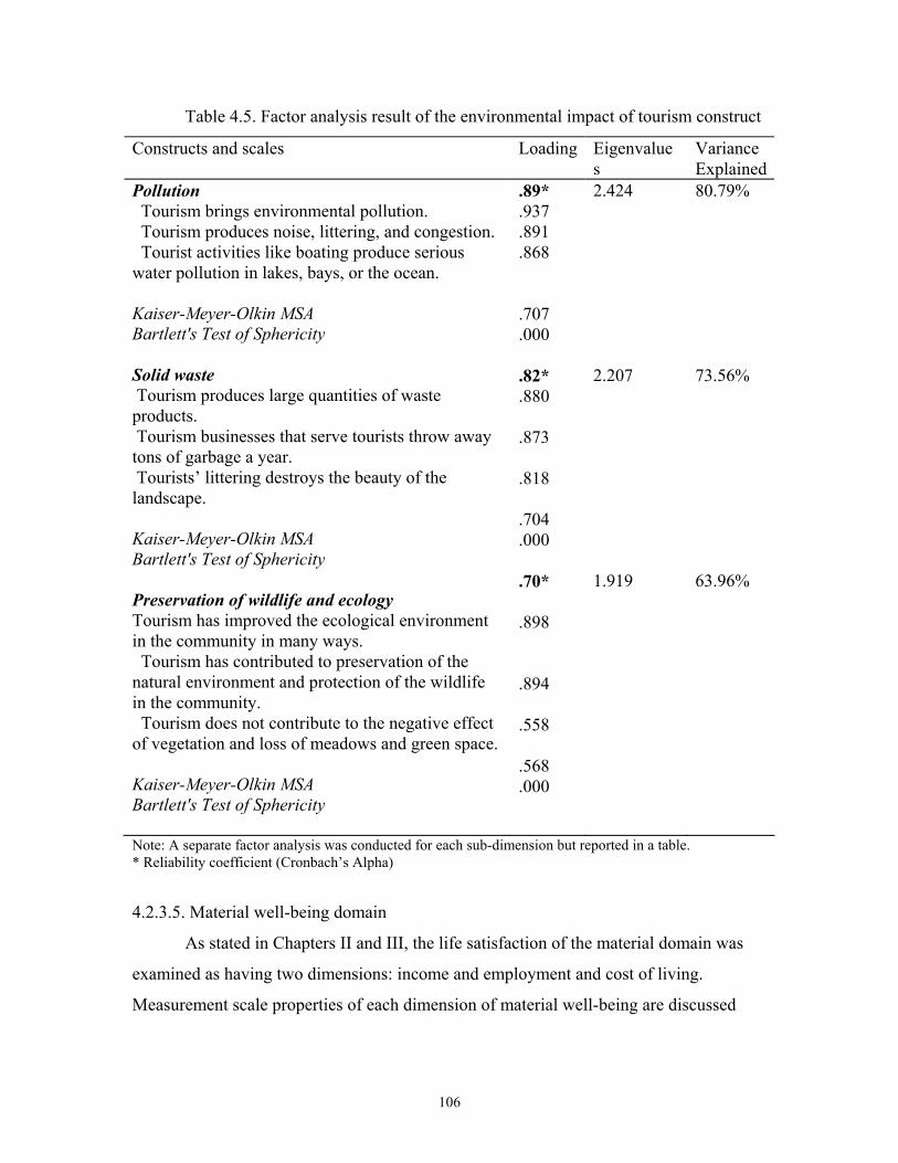
106
Table 4.5. Factor analysis result of the environmental impact of tourism construct
Constructs and scales Loading Eigenvalues
Variance Explained
Pollution Tourism brings environmental pollution. Tourism produces noise, littering, and congestion. Tourist activities like boating produce serious water pollution in lakes, bays, or the ocean. Kaiser-Meyer-Olkin MSA Bartlett's Test of Sphericity Solid waste Tourism produces large quantities of waste products. Tourism businesses that serve tourists throw away tons of garbage a year. Tourists’ littering destroys the beauty of the landscape. Kaiser-Meyer-Olkin MSA Bartlett's Test of Sphericity Preservation of wildlife and ecology Tourism has improved the ecological environment in the community in many ways. Tourism has contributed to preservation of the natural environment and protection of the wildlife in the community. Tourism does not contribute to the negative effect of vegetation and loss of meadows and green space. Kaiser-Meyer-Olkin MSA Bartlett's Test of Sphericity
.89*
.937
.891
.868 .707 .000 .82* .880 .873 .818 .704 .000 .70* .898 .894 .558 .568 .000
2.424 2.207 1.919
80.79% 73.56% 63.96%
Note: A separate factor analysis was conducted for each sub-dimension but reported in a table. * Reliability coefficient (Cronbach’s Alpha)
4.2.3.5. Material well-being domain
As stated in Chapters II and III, the life satisfaction of the material domain was
examined as having two dimensions: income and employment and cost of living.
Measurement scale properties of each dimension of material well-being are discussed
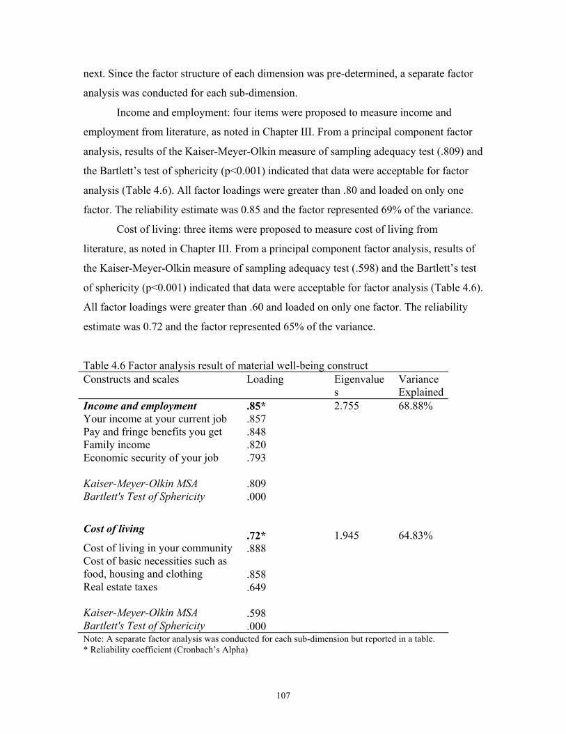
107
next. Since the factor structure of each dimension was pre-determined, a separate factor
analysis was conducted for each sub-dimension.
Income and employment: four items were proposed to measure income and
employment from literature, as noted in Chapter III. From a principal component factor
analysis, results of the Kaiser-Meyer-Olkin measure of sampling adequacy test (.809) and
the Bartlett’s test of sphericity (p<0.001) indicated that data were acceptable for factor
analysis (Table 4.6). All factor loadings were greater than .80 and loaded on only one
factor. The reliability estimate was 0.85 and the factor represented 69% of the variance.
Cost of living: three items were proposed to measure cost of living from
literature, as noted in Chapter III. From a principal component factor analysis, results of
the Kaiser-Meyer-Olkin measure of sampling adequacy test (.598) and the Bartlett’s test
of sphericity (p<0.001) indicated that data were acceptable for factor analysis (Table 4.6).
All factor loadings were greater than .60 and loaded on only one factor. The reliability
estimate was 0.72 and the factor represented 65% of the variance.
Table 4.6 Factor analysis result of material well-being construct Constructs and scales Loading Eigenvalue
s Variance Explained
Income and employment Your income at your current job Pay and fringe benefits you get Family income Economic security of your job Kaiser-Meyer-Olkin MSA Bartlett's Test of Sphericity
Cost of living
Cost of living in your community Cost of basic necessities such as food, housing and clothing Real estate taxes Kaiser-Meyer-Olkin MSA Bartlett's Test of Sphericity
.85*
.857
.848
.820
.793 .809 .000 .72* .888 .858 .649 .598 .000
2.755 1.945
68.88% 64.83%
Note: A separate factor analysis was conducted for each sub-dimension but reported in a table. * Reliability coefficient (Cronbach’s Alpha)
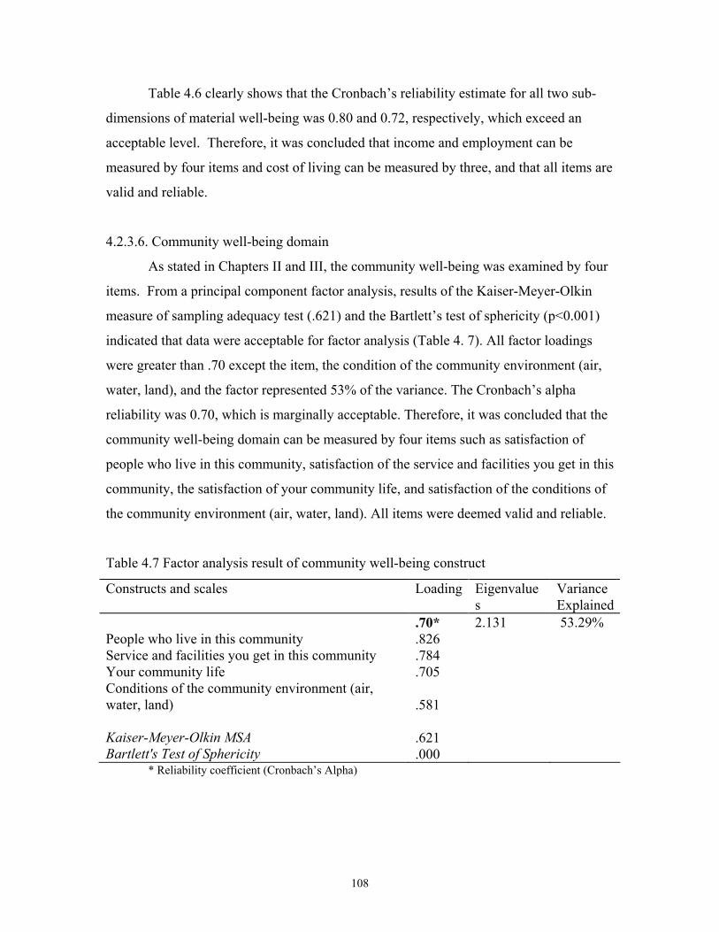
108
Table 4.6 clearly shows that the Cronbach’s reliability estimate for all two sub-
dimensions of material well-being was 0.80 and 0.72, respectively, which exceed an
acceptable level. Therefore, it was concluded that income and employment can be
measured by four items and cost of living can be measured by three, and that all items are
valid and reliable.
4.2.3.6. Community well-being domain
As stated in Chapters II and III, the community well-being was examined by four
items. From a principal component factor analysis, results of the Kaiser-Meyer-Olkin
measure of sampling adequacy test (.621) and the Bartlett’s test of sphericity (p<0.001)
indicated that data were acceptable for factor analysis (Table 4. 7). All factor loadings
were greater than .70 except the item, the condition of the community environment (air,
water, land), and the factor represented 53% of the variance. The Cronbach’s alpha
reliability was 0.70, which is marginally acceptable. Therefore, it was concluded that the
community well-being domain can be measured by four items such as satisfaction of
people who live in this community, satisfaction of the service and facilities you get in this
community, the satisfaction of your community life, and satisfaction of the conditions of
the community environment (air, water, land). All items were deemed valid and reliable.
Table 4.7 Factor analysis result of community well-being construct
Constructs and scales Loading Eigenvalues
Variance Explained
People who live in this community Service and facilities you get in this community Your community life Conditions of the community environment (air, water, land) Kaiser-Meyer-Olkin MSA Bartlett's Test of Sphericity
.70*
.826
.784
.705 .581 .621 .000
2.131
53.29%
* Reliability coefficient (Cronbach’s Alpha)

109
4.2.3.7. Emotional well-being domain
As stated in Chapter II and III, the emotional well-being domain was examined as
having two dimensions: leisure well-being and spiritual well-being domain. Measurement
scale properties of each dimension of the emotional well-being domain was discussed
next. Since the factor structure of each dimension was pre-determined, a separate factor
analysis was conducted for each sub-dimension.
Leisure well-being domain: four items were proposed to measure the leisure well-
being domain from literature, as noted in Chapter III. From a principal component factor
analysis, results of the Kaiser-Meyer-Olkin measure of sampling adequacy test (.673) and
the Bartlett’s test of sphericity (p<0.001) indicated that data were acceptable for factor
analysis (Table 4.8). All factor loadings were greater than .68 and loaded on only one
factor. The Cronbach’s alpha reliability was 0.82 and the factor represented 65% of the
variance.
Spiritual well-being domain: five items were proposed to measure the spiritual
well-being domain from literature, as noted in Chapter III. From a principal component
factor analysis, results of the Kaiser-Meyer-Olkin measure of sampling adequacy test
(.677) and the Bartlett’s test of sphericity (p<0.001) indicated that data were acceptable
for factor analysis (Table 4.8). The principal component analysis indicated that there
were two factors. However, only one item loaded on the second factor (Table 4.8). The
first factor represented 55% of the explained variance of the scale. The first factor was
comprised of four items with factor loadings greater than .60. Those items were: (1) I am
particularly happy with the way we preserve culture in my community, (2) Satisfaction
with cultural life, (3) I am very satisfied with the availabilities of religious services in my
community, (4) I feel I extend my cultural outlook when I talk with tourists (factor
loading of .791, .755, .648, and .634, respectively). The second factor could have
contributed an additional 21.35% to the explained variance of scales; however, the
objective of the pretest was to establish a unidimensional scale for the measurement of
the construct. Therefore, only items that loaded on the first factor were selected. The
Cronbach’s alpha reliability indicated that the coefficient was 0.66, which is marginally
acceptable.
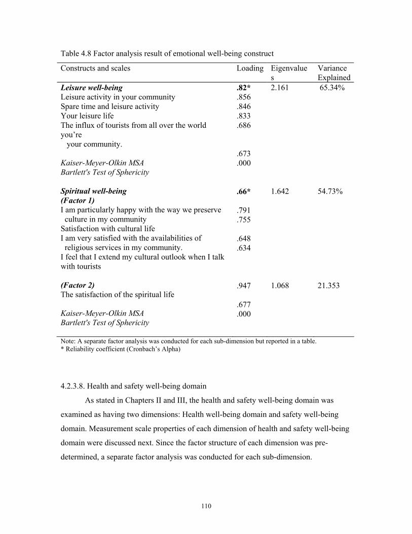
110
Table 4.8 Factor analysis result of emotional well-being construct
Constructs and scales Loading Eigenvalues
Variance Explained
Leisure well-being Leisure activity in your community Spare time and leisure activity Your leisure life The influx of tourists from all over the world you’re your community. Kaiser-Meyer-Olkin MSA Bartlett's Test of Sphericity Spiritual well-being (Factor 1) I am particularly happy with the way we preserve culture in my community Satisfaction with cultural life I am very satisfied with the availabilities of religious services in my community. I feel that I extend my cultural outlook when I talk with tourists (Factor 2) The satisfaction of the spiritual life Kaiser-Meyer-Olkin MSA Bartlett's Test of Sphericity
.82*
.856
.846
.833
.686 .673 .000 .66* .791 .755 .648 .634 .947 .677 .000
2.161 1.642 1.068
65.34% 54.73% 21.353
Note: A separate factor analysis was conducted for each sub-dimension but reported in a table. * Reliability coefficient (Cronbach’s Alpha)
4.2.3.8. Health and safety well-being domain
As stated in Chapters II and III, the health and safety well-being domain was
examined as having two dimensions: Health well-being domain and safety well-being
domain. Measurement scale properties of each dimension of health and safety well-being
domain were discussed next. Since the factor structure of each dimension was pre-
determined, a separate factor analysis was conducted for each sub-dimension.
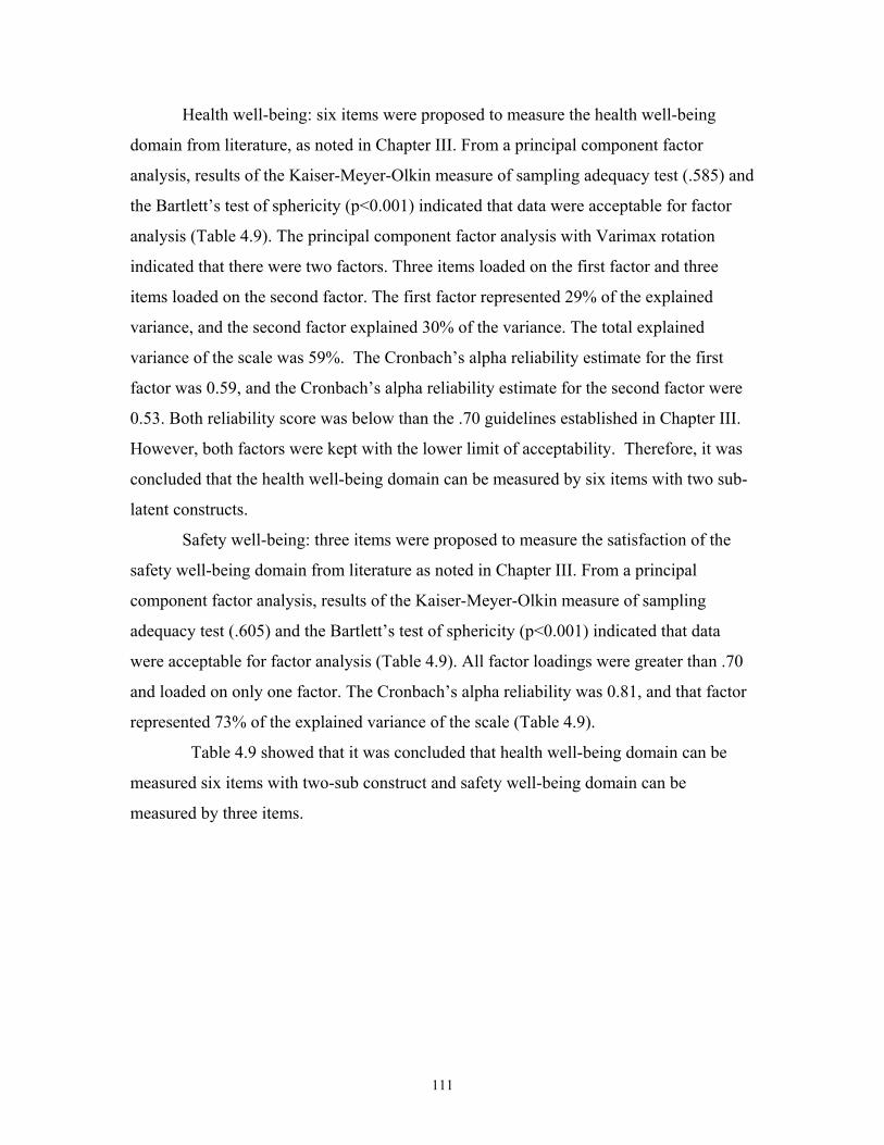
111
Health well-being: six items were proposed to measure the health well-being
domain from literature, as noted in Chapter III. From a principal component factor
analysis, results of the Kaiser-Meyer-Olkin measure of sampling adequacy test (.585) and
the Bartlett’s test of sphericity (p<0.001) indicated that data were acceptable for factor
analysis (Table 4.9). The principal component factor analysis with Varimax rotation
indicated that there were two factors. Three items loaded on the first factor and three
items loaded on the second factor. The first factor represented 29% of the explained
variance, and the second factor explained 30% of the variance. The total explained
variance of the scale was 59%. The Cronbach’s alpha reliability estimate for the first
factor was 0.59, and the Cronbach’s alpha reliability estimate for the second factor were
0.53. Both reliability score was below than the .70 guidelines established in Chapter III.
However, both factors were kept with the lower limit of acceptability. Therefore, it was
concluded that the health well-being domain can be measured by six items with two sub-
latent constructs.
Safety well-being: three items were proposed to measure the satisfaction of the
safety well-being domain from literature as noted in Chapter III. From a principal
component factor analysis, results of the Kaiser-Meyer-Olkin measure of sampling
adequacy test (.605) and the Bartlett’s test of sphericity (p<0.001) indicated that data
were acceptable for factor analysis (Table 4.9). All factor loadings were greater than .70
and loaded on only one factor. The Cronbach’s alpha reliability was 0.81, and that factor
represented 73% of the explained variance of the scale (Table 4.9).
Table 4.9 showed that it was concluded that health well-being domain can be
measured six items with two-sub construct and safety well-being domain can be
measured by three items.
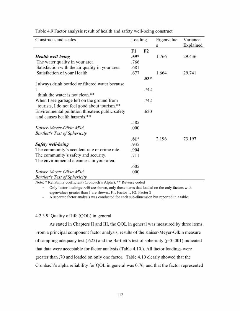
112
Table 4.9 Factor analysis result of health and safety well-being construct
Constructs and scales Loading Eigenvalues
Variance Explained
Health well-being The water quality in your area Satisfaction with the air quality in your area Satisfaction of your Health I always drink bottled or filtered water because I think the water is not clean.** When I see garbage left on the ground from tourists, I do not feel good about tourism.** Environmental pollution threatens public safety and causes health hazards.** Kaiser-Meyer-Olkin MSA Bartlett's Test of Sphericity Safety well-being The community’s accident rate or crime rate. The community’s safety and security. The environmental cleanness in your area. Kaiser-Meyer-Olkin MSA Bartlett's Test of Sphericity
F1 .59*.766.681.677 .585.000 .81*.935.904.711 .605.000
F2 .53* .742 .742 .620
1.766 1.664 2.196
29.436 29.741 73.197
Note: * Reliability coefficient (Cronbach’s Alpha), ** Reverse coded - Only factor loadings >.40 are shown, only those items that loaded on the only factors with
eigenvalues greater than 1 are shown., F1: Factor 1, F2: Factor 2 - A separate factor analysis was conducted for each sub-dimension but reported in a table.
4.2.3.9. Quality of life (QOL) in general
As stated in Chapters II and III, the QOL in general was measured by three items.
From a principal component factor analysis, results of the Kaiser-Meyer-Olkin measure
of sampling adequacy test (.625) and the Bartlett’s test of sphericity (p<0.001) indicated
that data were acceptable for factor analysis (Table 4.10.). All factor loadings were
greater than .70 and loaded on only one factor. Table 4.10 clearly showed that the
Cronbach’s alpha reliability for QOL in general was 0.76, and that the factor represented
113
68% of the explained variance of the scale. Therefore, it was concluded that quality of
life in general can be measured three items, and that all items are valid and reliable.
Table 4.10 Factor analysis result of the quality of life in general
Constructs and scales Loading Eigenvalues
Variance Explained
Your life as a whole The way you are spending your life How you feel about your life*** Kaiser-Meyer-Olkin MSA Bartlett's Test of Sphericity
.76*
.894
.863
.705 .625 .000
2.042
68.076
Note: * Reliability coefficient (Cronbach’s Alpha)
Through the pretest, all items to measure the tourism impact contracts, the
satisfaction of well-being domains, and quality of life in general were considered to be
reliable and valid.
4.3. FINAL SURVEY
This section of the chapter will discuss the final survey method, the sample, the
response rate, and the demographic characteristics of the final sample.
4.3.1. Survey method
A self-administered survey questionnaire was used to collect data. The
questionnaire was delivered via the U.S. Postal Service to a stratified random sample in
the different tourism development stages. The mailed package included a cover letter pre-
printed in the questionnaire booklet, a self-addressed and stamped envelope, and the
questionnaire (Appendix A). Two weeks after the first survey was mailed, a reminder
postcard was sent to the sample (Appendix B). Then, two weeks after the postcard was
sent, the second survey questionnaire was mailed.

114
4.3.2. Sample
The sample population consisted of individuals who reside in the pre-selected
destination in different developmental tourism stages in the State of Virginia. A survey
questionnaire with a pre-written cover letter was mailed to 2,400 residents in the pre-
selected destination of different developmental tourism stages. In order to make sure that
the sample represented the population distribution in the pre-selected destination in
different developmental tourism stages, a stratified sampling approach was used. First,
the total population of the pre-selected counties and cities of different developmental
tourism stages in Virginia was obtained from the U.S. Census Bureau (2002).
Afterwards, the number of respondents needed from each county and city to obtain a total
sample of 2,400 was calculated. Once the number of respondents was identified, a
random sampling method was used to select the appropriate number of respondents from
each pre-selected county and city. The sample (mailing list) for this study was
downloaded from the Reference USA database (http://www.referenceusa.com/)
residential information section. Appendix C presents the population of pre-selected
counties and cities and the number of respondents from each county and city.
The overall response rate was 13.76% (327 respondents) (See Table 4.11). Six of
the returned questionnaires were eliminated as the data were being coded because they
were returned blank or were only partially completed. After eliminating the unusable
responses, 321 responses were coded and used for data analysis.
Table 4.11 Response Rate
Number Percent Total target population 2,400 100.00% Undeliverable 24 1.00% Total survey population 2376 99.00% Total survey population from above 2376 100.00% Total responses 327 13.76% Unusable 6 0.25% Total usable responses 321 13.51% Description of unusable surveys Returned without any completion
4
Incomplete surveys 2
115
A general overview of the respondents follows. For more specific details
regarding the age, income, ethnic group, gender and the type of occupation, household
status, and the number of people in the household, please refer to the profile of the
respondents shown in Appendix D.
4.3.3. Profile of the respondents
The demographic characteristics of age, education, gender, ethnic group, and
income were included in this chapter in an effort to provide a descriptive profile of the
survey respondents. A discussion of the demographic characteristics ensues.
Age
Survey respondents were asked their age in an open-ended question, and were
provided a blank in which to supply the answer. Most the people who returned completed
questionnaires (48.1%) were 55 or older; around 41.4% of the respondents were between
the ages of 35 and 54. The average age of the respondents was 53.6 years old. The
standard deviation of age was 15 years old.
Gender
Survey respondents were asked to circle if they were male (M) or female (F).
More than half of the respondents were men. Of the three hundred nineteen individuals
who provided gender information, 170 (53.3%) were male, whereas 149 (46.7%) were
female.
Ethnic origin
Respondents were asked to provide information regarding their ethnic origin by
circling one of the following choices: Caucasian, Hispanic, African-American, Asian,
and others. The vast majority of the survey participants were white (82.1%), with only
13.8% being African-American, 1% indicating Hispanic and Asian, and 2.2% presenting
others.

116
Income
Respondents were asked to circle their approximate household income. More of
the survey population left this question blank than any other question on the survey, with
only 292 of the 321 respondents providing information regarding their annual income. Of
those who did answer the question, 12.3% reported income less than $20,000, whereas
11.3% reported incomes in excess of $100,000. Most of the reported incomes fell
between $20,001 to $60,000, with 21.9% of the respondents reporting incomes between
$20,001 and $40,000, and 19.2% indicating that they earned between $40,001 and
$60,000. 22.6% of survey respondents indicated that they earned between $60,001 and
$80,000 annually. Surprisingly, 24% of the respondents reported incomes in excess of
$80,001, with 12.7% declaring incomes between $80,000 and $100,000 and 11.3
reporting incomes in excess of $100,001.
Years of residency in community
Length of residency in the study area averaged 22.34 years for the respondents.
The majority of the respondents (44.6%) have lived in their present community for over
20 years. Another 19.3% had resided in the same locality for 11 to 20 years. 19.9%
reported a length of residency of 10 years or less.
Subjective perception of tourism development
To crosscheck the selected area for the objective tourism development stage by
using the secondary indicators, the respondents were asked to present their subjective
feeling of tourism development stages in their community. Among 286 respondents, 50%
of the respondents answered that they felt their community falls in the growth stages; the
rest of the respondents answered that they felt their community falls either in the maturity
stage (22%), beginning stage (20.6%), or decline stage (7.3%). Table 4. 12 showed the
frequencies comparing the subjective development stage and objective development
stages. The chi-square test was statistically significant at α=0.05 levels, but most
residents from the objectively assigned tourism development stage areas felt that their
community falls in the maturity stage of tourism development. Only 52.4% of the
respondents from decline stage areas felt that their community falls in the decline stage.
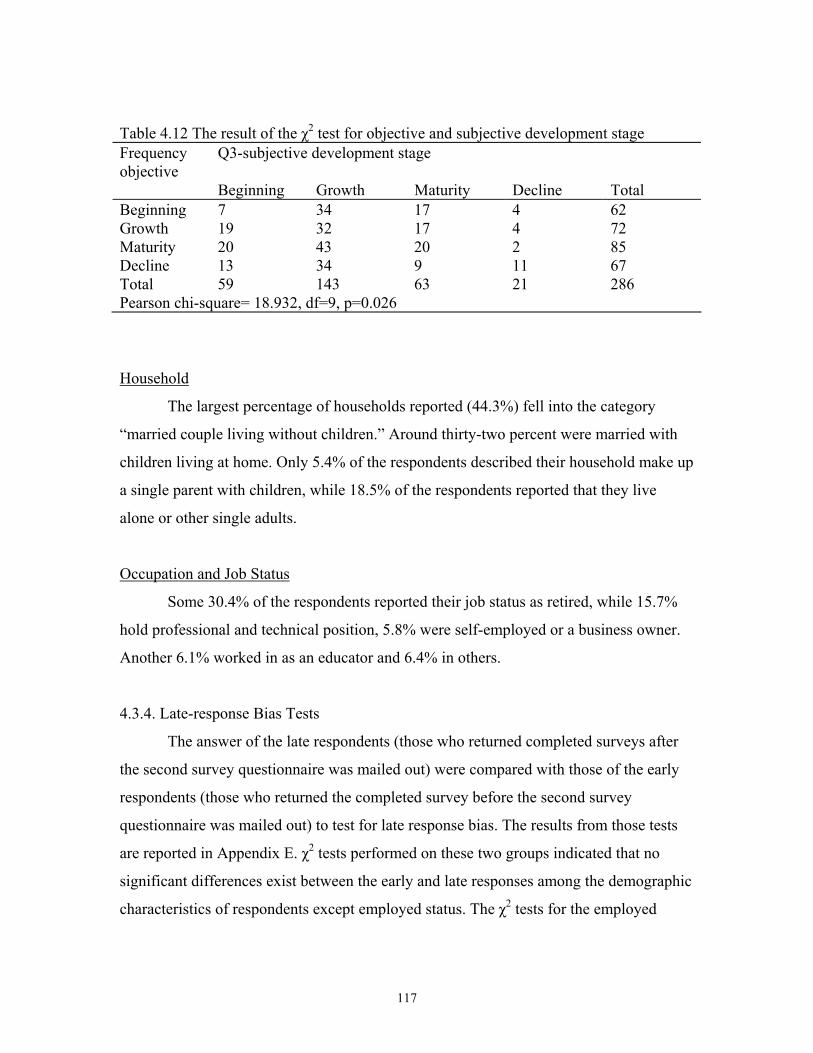
117
Table 4.12 The result of the χ2 test for objective and subjective development stage Frequency objective
Q3-subjective development stage
Beginning Growth Maturity Decline Total Beginning 7 34 17 4 62 Growth 19 32 17 4 72 Maturity 20 43 20 2 85 Decline 13 34 9 11 67 Total 59 143 63 21 286 Pearson chi-square= 18.932, df=9, p=0.026
Household
The largest percentage of households reported (44.3%) fell into the category
“married couple living without children.” Around thirty-two percent were married with
children living at home. Only 5.4% of the respondents described their household make up
a single parent with children, while 18.5% of the respondents reported that they live
alone or other single adults.
Occupation and Job Status
Some 30.4% of the respondents reported their job status as retired, while 15.7%
hold professional and technical position, 5.8% were self-employed or a business owner.
Another 6.1% worked in as an educator and 6.4% in others.
4.3.4. Late-response Bias Tests
The answer of the late respondents (those who returned completed surveys after
the second survey questionnaire was mailed out) were compared with those of the early
respondents (those who returned the completed survey before the second survey
questionnaire was mailed out) to test for late response bias. The results from those tests
are reported in Appendix E. χ2 tests performed on these two groups indicated that no
significant differences exist between the early and late responses among the demographic
characteristics of respondents except employed status. The χ2 tests for the employed
118
status showed the significant difference between early and late respondent group at
α=0.05 levels.
4.3.5 Descriptive Statistics, Skewness, and Kurtosis
Since all of the data had been keyed into SPSS by hand, before any tests were
conducted using the data set, frequency distributions for each variable in the study were
run and examined to ensure that the data were “clean.” As could be expected, a few
keying errors were evident, and the actual survey questionnaires corresponding with the
survey coding number for the surveys that contained coding errors were pulled. The
errors were corrected and frequencies were run a second time to ensure that all of the
keying errors had been corrected. Next, measures of central tendency were run for each
of the variables in the study. The mean scores and standard deviations in addition to the
skewness and kurtosis of each of the variables in the study are shown in Appendix F.
To assess the normality of the distribution of the data, the skewness and kurtosis
of each variable were examined. The critical value for both of these measures of
normality is drawn from a z distribution. The SPSS software package was used to
generate the skewness and kurtosis values for each of the variables in the model.
Therefore, for the calculated skewness and kurtosis values, zero assumes perfect
normality in the data distribution (which is seldom achieved), ± 2.58 indicating rejecting
the normality assumption at the 0.01 probability level, and ± 1.96 signifies a 0.05 error
level (Hair et al. 1998). By applying the above criteria to the skewness values for each of
the variables listed in Appendix F, it is clear that no variable fell outside the ±1.96 range
for skewness. Therefore, it can be assumed that all of the variables for the study are
reasonably free from skewness.
Another data characteristic that was considered is the kurtosis: how observations
“cluster around a central point” for a given standard distribution (Norusis, 1990, p.82).
Distributions that are more peaked than normal are called “leptokurtic,” whereas those
that are flatter than normal are referred to as “platykurtic.” Positive values for kurtosis
show that a distribution has a higher than normal peak. Looking again at Appendix F,
none of the variables fell outside ±2.56 range for kurtosis. Therefore, the study can
conclude that none of variables was leptokurtic or platykurtic.

119
4.4 DATA ANALYSIS
This section of the chapter will present the results of the statistical analysis of the
data collected. First, the results of the confirmatory analysis of the constructs which have
sub-dimensions is presented. After confirming the each sub-dimension of the constructs,
a summated scale is constructed for each construct. For example, the economic impact of
tourism has four sub-dimensions. After confirming four sub-dimensions of the economic
impact construct, the economic impact of tourism was examined as one construct by
using each summated scale as a measurement item of the economic impact of tourism
construct as discussed in Chapter III. Next, the result of the measurement model,
including all constructs, is presented. Afterwards, the results of the structural equation
modeling will be presented to test the proposed hypotheses.
4.4.1 Confirmatory factor analysis
The preceding section of Chapter IV presented the pretest results of the proposed
measurement scale for each dimension of economic impact of tourism and for other
scales that were proposed other constructs. The next step in the analysis was to perform a
confirmatory factor analysis to confirm the measurement scale properties. As stated
earlier and in Chapter III, a summated scale is used to measure the economic impact of
tourism construct. The indicators of each sub-dimension of economic impact of tourism
were summated, and the resulting four summated scales were used to measure the
economic impact of tourism. However, before testing the measurement model properties
of the whole proposed measurement model, a separate confirmatory factor analysis is
required to perform on each sub-dimension of the nine constructs to check the reliability
and validity of the indicators. The observed variables that were grouped together in the
component factor analysis (in pretest) were utilized to perform the confirmatory factor
analysis.
The reliability of the variables is defined as the square of the correlation between
a latent factor and the indicators. In other words, the reliability indicates the percent of
variation in the indicator that is explained by the factor that it is supposed to measure
(Long, 1983a). On the other hand, the validity refers to whether an instrument measures
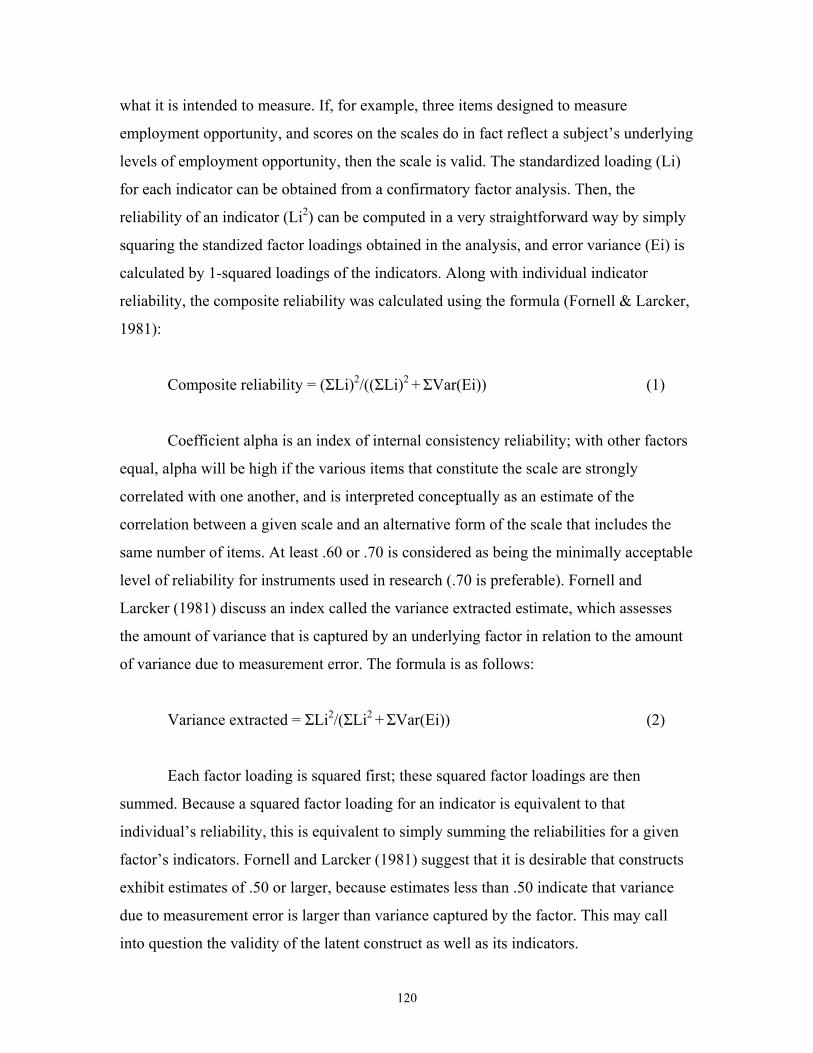
120
what it is intended to measure. If, for example, three items designed to measure
employment opportunity, and scores on the scales do in fact reflect a subject’s underlying
levels of employment opportunity, then the scale is valid. The standardized loading (Li)
for each indicator can be obtained from a confirmatory factor analysis. Then, the
reliability of an indicator (Li2) can be computed in a very straightforward way by simply
squaring the standized factor loadings obtained in the analysis, and error variance (Ei) is
calculated by 1-squared loadings of the indicators. Along with individual indicator
reliability, the composite reliability was calculated using the formula (Fornell & Larcker,
1981):
Composite reliability = (ΣLi)2/((ΣLi)2 + ΣVar(Ei)) (1)
Coefficient alpha is an index of internal consistency reliability; with other factors
equal, alpha will be high if the various items that constitute the scale are strongly
correlated with one another, and is interpreted conceptually as an estimate of the
correlation between a given scale and an alternative form of the scale that includes the
same number of items. At least .60 or .70 is considered as being the minimally acceptable
level of reliability for instruments used in research (.70 is preferable). Fornell and
Larcker (1981) discuss an index called the variance extracted estimate, which assesses
the amount of variance that is captured by an underlying factor in relation to the amount
of variance due to measurement error. The formula is as follows:
Variance extracted = ΣLi2/(ΣLi2 + ΣVar(Ei)) (2)
Each factor loading is squared first; these squared factor loadings are then
summed. Because a squared factor loading for an indicator is equivalent to that
individual’s reliability, this is equivalent to simply summing the reliabilities for a given
factor’s indicators. Fornell and Larcker (1981) suggest that it is desirable that constructs
exhibit estimates of .50 or larger, because estimates less than .50 indicate that variance
due to measurement error is larger than variance captured by the factor. This may call
into question the validity of the latent construct as well as its indicators.
121
4.4.1.1 Confirmatory factor analysis of economic impact of tourism constructs
Before testing the overall confirmatory measurement model, the measurement
unidimensionality of each sub-dimension of the economic impact of tourism and other
constructs was assessed individually. First, four dimensions of the economic impact of
tourism were discussed in detail in Chapter II. A measurement scale was proposed to
assess each dimension in Chapter III. The confirmatory factor analysis was performed by
specifying the posited relationships of the observed variables to the underlying four
dimensions of economic impact of tourism, with the dimensions allowed to intercorrelate
freely. The covariance matrix was used as the input data for the confirmatory factor
analysis procedure available in LISREL 8.3 (Jöreskog & Sorbom, 1989).
The confirmatory measurement model to be tested postulates a priori that the
economic impact of tourism is a four-factor structure composed of (1) employment
opportunity, (2) revenue from tourists for local business and government, (3) standard of
living, and (4) cost of living. Further dissection of the model indicates that these four
factors are correlated and that there were 13 observed variables. As shown in the pretest,
three observed variables loaded onto employment opportunity, standard of living, and
cost of living, and four observed variables loaded onto the building revenue from tourists
for local business and government. In addition, errors of measurement associated with
each observed variable were uncorrelated. Before testing the overall confirmatory
measurement for the economic impact of tourism model, the measurement of each sub-
construct was assessed individually.
A separate confirmatory factor analysis was performed for each sub-construct
with three or more observed variables. If a construct had three observed variables, it was
combined with another construct and a confirmatory factor analysis was performed for
both constructs. If model fit was unacceptable, the modification indices and residuals
were examined. Based on the suggestions of the modification indices and the size of
residuals, constructs with acceptable fit were respecified to increase model fit by deleting
the indicators that had large residuals (over 2.56, Hair et al., 1998) and/or wanted to load
on other constructs (greater than 3.89, Hair et al, 1998). Assessing each sub-dimension of
economic impact of tourism construct individually resulted in no change to the indicators
122
in the sub-dimensions, and results indicated that all four sub-dimensions had
measurement unidimensionality. After assessing the unidimensionality of each sub-
dimension individually, a measurement model for each pair of constructs was estimated,
combining them two by two. Afterwards, the overall measurement fit of the economic
impact of the tourism construct was tested by a confirmatory factor analysis. The items
and the result of the confirmatory factor analysis of sub-dimension of the economic
impact of tourism are presented in Table 4.13. Table 4.13 presents the completely
standized coefficients (i.e., both the latent and observed variables are standized), the
indicator reliabilities (i.e., the squared multiple correlation for X-variables), and the error
variances for each indicator. The composite indicator reliabilities and variance extracted
estimates were calculated using the formula recommended by Fornell and Larcker
(1981). As presented in table 4.13, all of the composite reliabilities were above .7 and all
variance extracted estimates were above.5. The overall fit of this final measurement
model of the economic impact of tourism construct was χ2(59)= 125.98 (p=0.00);
GFI=0.94; AGFI=0.91; PGFI=0.61; IFI=0.97; NNFI=0.95; CFI=0.97; RFI=0.92; AND
Critical N=211.4. Further, the indicators of residuals, standized RMR (SRMR) and root
mean squared error of approximation (RMSEA) were 0.033 and 0.066, respectively.
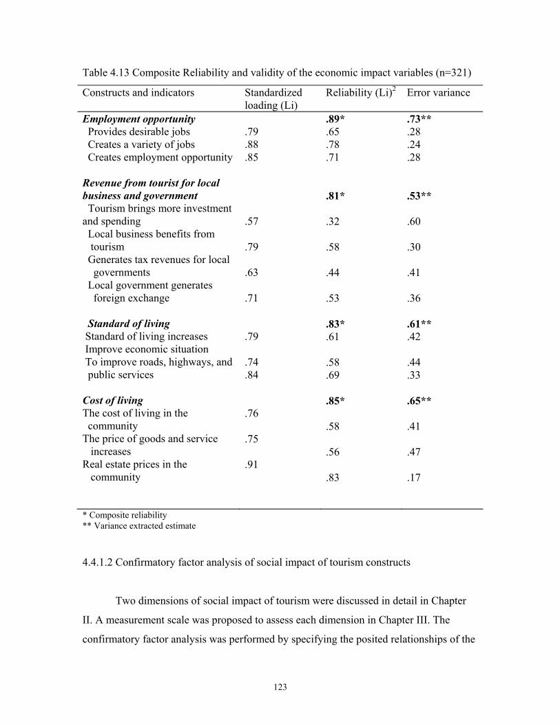
123
Table 4.13 Composite Reliability and validity of the economic impact variables (n=321)
Constructs and indicators Standardized loading (Li)
Reliability (Li)2 Error variance
Employment opportunity Provides desirable jobs Creates a variety of jobs Creates employment opportunity Revenue from tourist for local business and government Tourism brings more investment and spending Local business benefits from tourism Generates tax revenues for local governments Local government generates foreign exchange Standard of living Standard of living increases Improve economic situation To improve roads, highways, and public services Cost of living The cost of living in the community The price of goods and service increases Real estate prices in the community
.79 .88 .85 .57 .79 .63 .71 .79 .74 .84 .76 .75 .91
.89*
.65
.78
.71 .81* .32 .58 .44 .53 .83* .61 .58 .69 .85* .58 .56 .83
.73**
.28
.24
.28 .53** .60 .30 .41 .36 .61** .42 .44 .33 .65** .41 .47 .17
* Composite reliability ** Variance extracted estimate
4.4.1.2 Confirmatory factor analysis of social impact of tourism constructs
Two dimensions of social impact of tourism were discussed in detail in Chapter
II. A measurement scale was proposed to assess each dimension in Chapter III. The
confirmatory factor analysis was performed by specifying the posited relationships of the

124
observed variables to the underlying two dimensions of social impact of tourism, with the
dimensions allowed to intercorrelate freely. The covariance matrix was used as the input
data for the confirmatory factor analysis; the confirmatory measurement model to be
tested postulates a priori that social impact of tourism is a two-factor structure composed
of (1) social problem (5 indicators) (2) local service (3 indicators). Further dissection of
the model indicates that these two factors are correlated and there were 8 observed
variables. As shown in the pretest, five observed variables loaded onto social problem
and three indicators loaded onto local service. Assessing each sub-dimension of social
impact of tourism construct individually resulted in no change of the indicators in the
sub-dimensions, and results indicated that two sub-dimensions had measurement
unidimensionality. After assessing the unidimensionality of each sub-dimension
individually, the overall measurement fit of the social impact of the tourism construct
was tested by a confirmatory factor analysis. The items and the result of the confirmatory
factor analysis of sub-dimension of the social impact of tourism are presented in Table
4.14. As presented in table 4.14, all of the composite reliabilities were above .7 and all
variance-extracted estimates were above.5. The overall fit of this final measurement
model of the social impact of tourism construct was χ2(19)= 41.74 (p=0.0019); GFI=0.95;
AGFI=0.91; PGFI=0.50; IFI=0.97; NNFI=0.96; CFI=0.97; RFI=0.92; and Critical
N=170.84. The indicators of residuals, Standardized RMR (SRMR) and root mean
squared error of approximation (RMSEA) were 0.056 and 0.078, respectively.
Therefore, the summated scale for each sub-construct was calculated to measure the
social impact of tourism construct.
4.4.1.3 Confirmatory factor analysis of cultural impact of tourism constructs
Three dimensions of the cultural impact of tourism were discussed in detail in
Chapter II. A measurement scale was proposed to assess each dimension in Chapter III.
The confirmatory factor analysis was performed by specifying the posited relationships
of the observed variables to the underlying three dimensions of cultural impact of
tourism, with the dimensions allowed to intercorrelate freely.

125
Table 4.14. Composite Reliability and validity of the social impact variables Constructs and indicators Standardized
loading (Li) Reliability (Li)2 Error variance
Social problem For peak season, harder to get ticket. Resulted in unpleasantly overcrowded hike trail Resulted in unpleasantly overcrowded park Resulted in unpleasantly overcrowded shopping place Contributes social problem such as crime. Local Service Increased tourism provides more recreational opportunities for local residents Because of tourism, roads and other local services are well maintained Tourism is a major reason for the variety of entertainment in the community
.67 .91 .91 .82 .57 .67 .78 .79
.89* .45 .83 .82 .68 .32 .79* .45 .61 .62
.63** .55 .17 .18 .32 .68 .56** .55 .39 .38
* Composite reliability ** Variance extracted estimate
The covariance matrix was used as the input data, and the confirmatory measurement
model to be tested postulates a priori that the cultural impact of tourism is a three-factor
structure composed of (1) preservation of local service (3 indicators), (2) deterioration of
local service with 3 indicators, and (3) cultural exchange (4 items). Unlike the results in
the pretest, the occurrence of a loading for deterioration of local service (X6; tourism
causes the disruption of traditional cultural behavior patterns in local residents) was
greater than 1.0. Therefore, it was deleted before the goodness-of-fit was assessed. After
this procedure was repeated several times, the four observed indicators were selected to
measure the cultural impact of tourism. The overall fit of this final measurement model of
the cultural impact of tourism construct was χ2(2)= 7.85 (p=0.020); GFI=0.99;

126
AGFI=0.94; PGFI=0.20; IFI=0.99; NNFI=0.97; CFI=0.99; RFI=0.96; AND Critical
N=350.36. The indicators of residuals, SRMR and RMSEA were 0.018 and 0.096 (that is
higher than suggested acceptable fit but it was kept), respectively. The result of the
composite reliability and variance-extracted estimate for the cultural impact construct is
presented in Table 4.15.
Table 4.15.Composite Reliability and validity of the cultural impact variables
Constructs and indicators Standardized loading (Li)
Reliability (Li)2 Error variance
Meeting tourists from all over the world is definitely a life-enriching experience. The cultural exchange between residents and tourists is valuable for the residents. The cultural exchange between residents and tourists is pleasant for the residents. I would like to meet tourists from as many countries as possible in order to learn about their culture.
.78 .91 .80 .70
.88* .61 .83 .65 .48
.64** .39 .17 .35 .52
* Composite reliability ** Variance extracted estimate
4.4.1.4 Confirmatory factor analysis of the environmental impact of tourism construct
Three dimensions of the environmental impact of tourism were discussed in detail
in Chapter II. A measurement scale was proposed to assess each dimension in Chapter
III. The confirmatory factor analysis was performed by specifying the posited
relationships of the observed variables to the underlying three dimensions of the
environmental impact of tourism, with the dimensions allowed to intercorrelate freely.
The covariance matrix was used as the input data for the confirmatory factor analysis and
the confirmatory measurement model to be tested postulates a priori that social impact of
127
tourism is a three-factor structure composed of (1) pollution (5 indicators), (2) solid
waste (3 indicators), and preservation of wildlife and ecology (3 indicators). Assessing
each sub-dimension of the environmental impact of tourism construct individually, and
deleting indicators that had large residuals or wanted to load on other constructs, resulted
in decreases in the number of indicator in three constructs. The number of indicators used
to measure pollution decreased to three observed variables from five. The number of
indicators used to measure preservation of wildlife and ecology decreased to two
observed indicators from three. After assessing the unidimensionality of each sub-
dimension individually, the overall measurement fit of the environmental impact of the
tourism construct was tested by a confirmatory factor analysis. The items and the result
of the confirmatory factor analysis of sub-dimension of the environmental impact of
tourism are presented in Table 4.16. Table 4.16 presents the completely standardized
coefficients, the indicator reliability, error variance, the composite reliability and
variance-extracted estimate were calculated by using the formulary recommended by
Fornell and Larcker (1981). As presented in table 4.16, all of the composite reliabilities
were above .7 and all variance-extracted estimates were above.5. The overall fit of this
final measurement model of the social impact of tourism construct was χ2(17)= 36.47
(p=0.0040); GFI=0.96; AGFI=0.91; PGFI=0.45; IFI=0.97; NNFI=0.95; CFI=0.97;
RFI=0.93; AND Critical N=150.03. The indicators of residuals, standardized RMR
(SRMR) and root mean squared error of approximation (RMSEA) were 0.030 and 0.076,
respectively. Therefore, the summated scale for each sub-construct was calculated to
measure the environmental impact of tourism construct.
4.4.1.5 Confirmatory factor analysis of the material well-being construct
Two dimensions of the material well-being domain construct were discussed in
detail in Chapter II. A measurement scale was proposed to assess each dimension in
Chapter III. The confirmatory factor analysis was performed by specifying the posited
relationships of the observed variables to the underlying two dimensions of the material
well-being construct, with the dimensions allowed to intercorrelate freely.
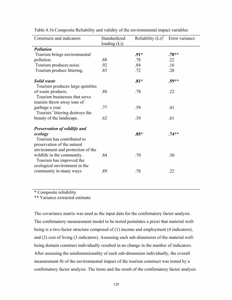
128
Table 4.16.Composite Reliability and validity of the environmental impact variables
Constructs and indicators Standardized loading (Li)
Reliability (Li)2 Error variance
Pollution Tourism brings environmental pollution. Tourism produces noise. Tourism produce littering. Solid waste Tourism produces large quintiles of waste products. Tourism businesses that serve tourists throw away tons of garbage a year. Tourists’ littering destroys the beauty of the landscape. Preservation of wildlife and ecology Tourism has contributed to preservation of the natural environment and protection of the wildlife in the community. Tourism has improved the ecological environment in the community in many ways.
.88 .92 .85 .88 .77 .62 .84 .89
.91* .78 .84 .72 .81* .78 .59 .39 .85* .70 .78
.78** .22 .16 .28 .59** .22 .41 .61 .74** .30 .22
* Composite reliability ** Variance extracted estimate
The covariance matrix was used as the input data for the confirmatory factor analysis.
The confirmatory measurement model to be tested postulates a priori that material well-
being is a two-factor structure composed of (1) income and employment (4 indicators),
and (2) cost of living (3 indicators). Assessing each sub-dimension of the material well-
being domain construct individually resulted in no change in the number of indicators.
After assessing the unidimensionality of each sub-dimension individually, the overall
measurement fit of the environmental impact of the tourism construct was tested by a
confirmatory factor analysis. The items and the result of the confirmatory factor analysis
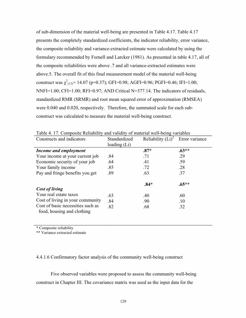
129
of sub-dimension of the material well-being are presented in Table 4.17. Table 4.17
presents the completely standardized coefficients, the indicator reliability, error variance,
the composite reliability and variance-extracted estimate were calculated by using the
formulary recommended by Fornell and Larcker (1981). As presented in table 4.17, all of
the composite reliabilities were above .7 and all variance-extracted estimates were
above.5. The overall fit of this final measurement model of the material well-being
construct was χ2(13)= 14.07 (p=0.37); GFI=0.98; AGFI=0.96; PGFI=0.46; IFI=1.00;
NNFI=1.00; CFI=1.00; RFI=0.97; AND Critical N=377.14. The indicators of residuals,
standardized RMR (SRMR) and root mean squared error of approximation (RMSEA)
were 0.040 and 0.020, respectively. Therefore, the summated scale for each sub-
construct was calculated to measure the material well-being construct.
Table 4. 17. Composite Reliability and validity of material well-being variables Constructs and indicators Standardized
loading (Li) Reliability (Li)2 Error variance
Income and employment Your income at your current job Economic security of your job Your family income Pay and fringe benefits you get Cost of living Your real estate taxes Cost of living in your community Cost of basic necessities such as food, housing and clothing
.84 .64 .85 .89 .63 .84 .82
.87*
.71
.41
.72
.63 .84* .40 .90 .68
.63**
.29
.59
.28
.37 .65** .60 .10 .32
* Composite reliability ** Variance extracted estimate
4.4.1.6 Confirmatory factor analysis of the community well-being construct
Five observed variables were proposed to assess the community well-being
construct in Chapter III. The covariance matrix was used as the input data for the
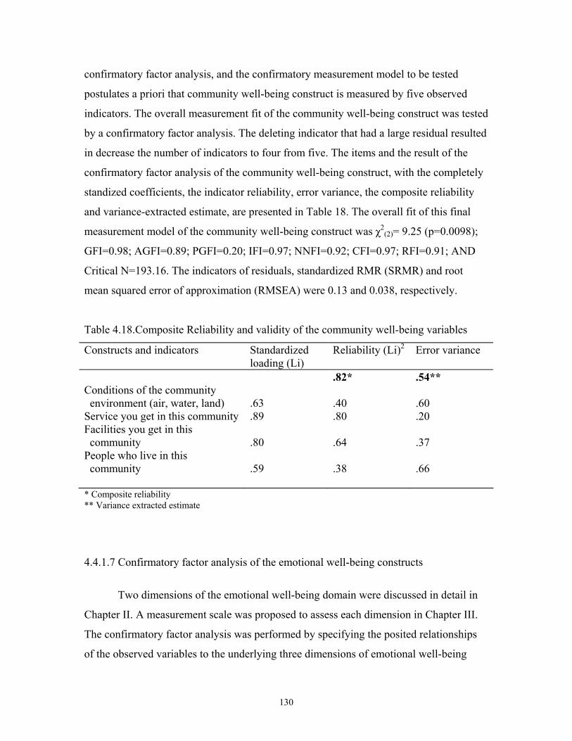
130
confirmatory factor analysis, and the confirmatory measurement model to be tested
postulates a priori that community well-being construct is measured by five observed
indicators. The overall measurement fit of the community well-being construct was tested
by a confirmatory factor analysis. The deleting indicator that had a large residual resulted
in decrease the number of indicators to four from five. The items and the result of the
confirmatory factor analysis of the community well-being construct, with the completely
standized coefficients, the indicator reliability, error variance, the composite reliability
and variance-extracted estimate, are presented in Table 18. The overall fit of this final
measurement model of the community well-being construct was χ2(2)= 9.25 (p=0.0098);
GFI=0.98; AGFI=0.89; PGFI=0.20; IFI=0.97; NNFI=0.92; CFI=0.97; RFI=0.91; AND
Critical N=193.16. The indicators of residuals, standardized RMR (SRMR) and root
mean squared error of approximation (RMSEA) were 0.13 and 0.038, respectively.
Table 4.18.Composite Reliability and validity of the community well-being variables
Constructs and indicators Standardized loading (Li)
Reliability (Li)2 Error variance
Conditions of the community environment (air, water, land) Service you get in this community Facilities you get in this community People who live in this community
.63 .89 .80 .59
.82* .40 .80 .64 .38
.54** .60 .20 .37 .66
* Composite reliability ** Variance extracted estimate
4.4.1.7 Confirmatory factor analysis of the emotional well-being constructs
Two dimensions of the emotional well-being domain were discussed in detail in
Chapter II. A measurement scale was proposed to assess each dimension in Chapter III.
The confirmatory factor analysis was performed by specifying the posited relationships
of the observed variables to the underlying three dimensions of emotional well-being
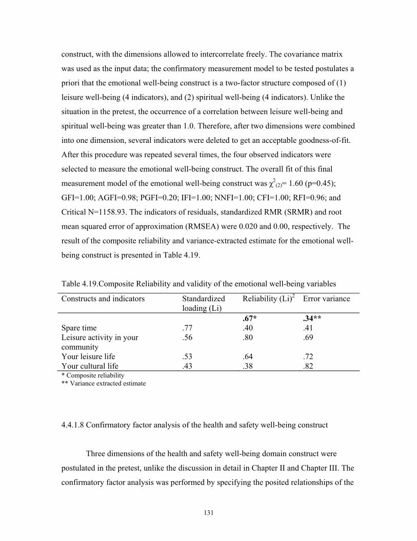
131
construct, with the dimensions allowed to intercorrelate freely. The covariance matrix
was used as the input data; the confirmatory measurement model to be tested postulates a
priori that the emotional well-being construct is a two-factor structure composed of (1)
leisure well-being (4 indicators), and (2) spiritual well-being (4 indicators). Unlike the
situation in the pretest, the occurrence of a correlation between leisure well-being and
spiritual well-being was greater than 1.0. Therefore, after two dimensions were combined
into one dimension, several indicators were deleted to get an acceptable goodness-of-fit.
After this procedure was repeated several times, the four observed indicators were
selected to measure the emotional well-being construct. The overall fit of this final
measurement model of the emotional well-being construct was χ2(2)= 1.60 (p=0.45);
GFI=1.00; AGFI=0.98; PGFI=0.20; IFI=1.00; NNFI=1.00; CFI=1.00; RFI=0.96; and
Critical N=1158.93. The indicators of residuals, standardized RMR (SRMR) and root
mean squared error of approximation (RMSEA) were 0.020 and 0.00, respectively. The
result of the composite reliability and variance-extracted estimate for the emotional well-
being construct is presented in Table 4.19.
Table 4.19.Composite Reliability and validity of the emotional well-being variables
Constructs and indicators Standardized loading (Li)
Reliability (Li)2 Error variance
Spare time Leisure activity in your community Your leisure life Your cultural life
.77 .56 .53 .43
.67*
.40
.80 .64 .38
.34**
.41
.69 .72 .82
* Composite reliability ** Variance extracted estimate
4.4.1.8 Confirmatory factor analysis of the health and safety well-being construct
Three dimensions of the health and safety well-being domain construct were
postulated in the pretest, unlike the discussion in detail in Chapter II and Chapter III. The
confirmatory factor analysis was performed by specifying the posited relationships of the
132
observed variables to the underlying three dimensions of the health and safety well-being
construct, with the dimensions allowed to intercorrelate freely. The covariance matrix
was used as the input data for the confirmatory factor analysis, and the confirmatory
measurement model to be tested postulates a priori that health and safety well-being is a
three-factor structure composed of (1) health well-being (3 indicators), (2) health concern
(3 indicators), and safety well-being (3indicators). Assessing each sub-dimension of the
health and safety and deleting indicators that had large error variance or/and large
residuals, and that wanted to load on other constructs, resulted in a decrease in the
number of indicators in the sub-dimensions. The number of sub-dimension was decreased
to two from three, and also, the number of indicators used to measure safety well-being
decreased to two from three. After assessing unidimensionality of each sub-dimension
individually, the overall measurement fit of the environmental impact of the tourism
construct was tested by a confirmatory factor analysis. The items and the result of the
confirmatory factor analysis of sub-dimension of the health and safety well-being
construct are presented in Table 4.20. Table 4.20 presents the completely standardized a
coefficient loading, the indicator reliability, error variance, the composite reliability and
variance-extracted estimate were calculated by using the formula recommended by
Fornell and Larcker (1981). Table 4.20 shows that the composite reliability for two sub-
dimension of the health and safety well-being construct had greater than .70 and
exceeded the requirement of acceptable level. Also, variance extracted estimate for all
sub-dimensions of the health and safety well-being was above .50, indicating that
variance due to measurement error is smaller than the variance captured by the factor.
Therefore, it was concluded that health well-being can be measured three items, and
safety well-being can be measured by two items. All items were deemed valid and
reliable. The overall fit of this final measurement model of the health and safety well-
being construct was χ2(4)= 6.62 (p=0.16); GFI=0.99; AGFI=0.95; PGFI=0.26; IFI=.99;
NNFI=.98; CFI=.99; RFI=0.95; and Critical N=393.20. The indicators of residuals,
standardized RMR (SRMR) and root mean squared error of approximation (RMSEA)
were 0.045 and 0.057, respectively. Therefore, the summated scale for each sub-
construct was calculated to measure the health and safety well-being construct.
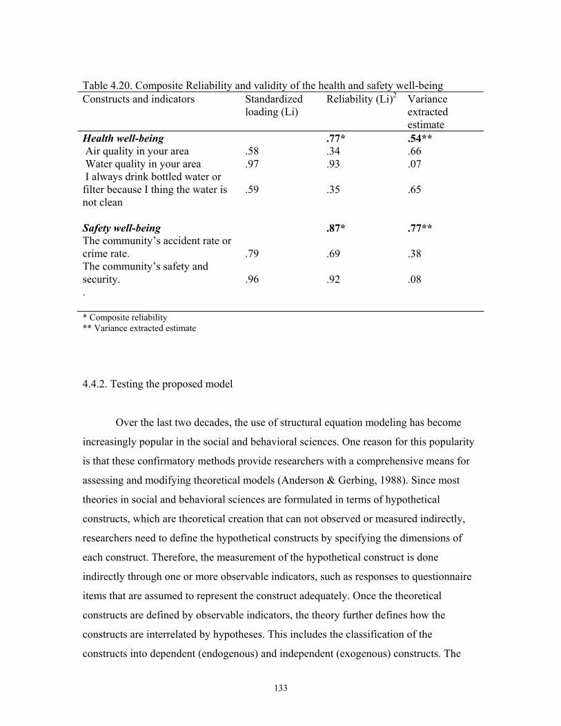
133
Table 4.20. Composite Reliability and validity of the health and safety well-being Constructs and indicators Standardized
loading (Li) Reliability (Li)2 Variance
extracted estimate
Health well-being Air quality in your area Water quality in your area I always drink bottled water or filter because I thing the water is not clean Safety well-being The community’s accident rate or crime rate. The community’s safety and security. .
.58 .97 .59 .79 .96
.77*
.34
.93 .35 .87* .69 .92
.54**
.66
.07 .65 .77** .38 .08
* Composite reliability ** Variance extracted estimate
4.4.2. Testing the proposed model
Over the last two decades, the use of structural equation modeling has become
increasingly popular in the social and behavioral sciences. One reason for this popularity
is that these confirmatory methods provide researchers with a comprehensive means for
assessing and modifying theoretical models (Anderson & Gerbing, 1988). Since most
theories in social and behavioral sciences are formulated in terms of hypothetical
constructs, which are theoretical creation that can not observed or measured indirectly,
researchers need to define the hypothetical constructs by specifying the dimensions of
each construct. Therefore, the measurement of the hypothetical construct is done
indirectly through one or more observable indicators, such as responses to questionnaire
items that are assumed to represent the construct adequately. Once the theoretical
constructs are defined by observable indicators, the theory further defines how the
constructs are interrelated by hypotheses. This includes the classification of the
constructs into dependent (endogenous) and independent (exogenous) constructs. The

134
relationship between observable indicators and the theoretical constructs constitutes the
measurement part of the model, and the theoretical relationship between the constructs
constitutes the structural part of the model (Jöreskog, 1993).
SEM is used to evaluate a substantive theory with empirical data through a
hypothesized model. The structural equation model presents a series of hypotheses about
how the variables are related. The parameters of the model are the regression coefficient
variance and covariance of variables. The commonly-used approaches to estimate the
parameters of structural equation models are maximum likelihood (ML) and normal
theory generalized least squires (GLS). Both estimation techniques assume that the
measured variables are continuous and have a multivariate normal distribution. However,
maximum likelihood estimation has been the most commonly-used approach in structural
equation modeling because ML estimations have been found to overcome the problems
created by the violations of normality, which means that estimates are good estimates,
even when the data are not normally distributed. However, all indicators that already
checked the normality showed that they have fair normal distribution (Appendix F).
Therefore, the properties of the items of nine constructs (four exogenous and five
endogenous) in the proposed model and the hypotheses were tested using the LISREL 8
structural equation analysis package (Jöreskog & Sorbom, 1993) with maximum
likelihood (ML) method of estimation (for recommendation for ML see Anderson &
Gerbing, 1988; Bentler, 1983), in combination with the two stage process recommended
by Sethi and King (1994) and Anderson and Gerbing (1988).
4.4.2.1. Measurement model
Maximum likelihood confirmatory factor analysis requires complete data for
every subject in order to preserve the integrity of the data set. The majority of the
variables had four or five missing cases. Therefore, cases with a missing value were
replaced with the mean value of that variable. A confirmatory factor analysis conducted
with a small sample size may result in inflated and spurious results. Monte Carlo studies
suggest that for relatively simple models (i.e., one, two, or three factors), a minimum of
100 subjects is required (Bearden, Sharma, & Teel, 1982). For more complex models,
substantially larger sample sizes are needed. With cases replaced by the mean value of
135
the variables, the total of 321 samples was kept and this sample size was considered large
enough to satisfy the sample size requirements of confirmatory factor analysis. Another
criterion requires that the correlation (or covariance) matrix include multiple measures of
each underlying constructs. In a single-factor model, at least three (ideally more)
observed measures (indicators) of the factor are required. In more complex (multiple-
factor) models, two measures per factor may be sufficient (Bryne, 1998; Hoyle, 1995).
All of the factors included in this study have at least two or three observed measures
(indicators).
Before testing the overall measurement model, measurement unidimensionality of
each construct was assessed individually (Sethi & King, 1994) because it is important to
make sure that the measures that are posited as alternate indicators of each construct are
acceptably unidimensional. Unidimensionality of constructs that are measured by at least
four observed indicators were tested individually. Unidimensionality of constructs that
are measured by less than four observed indicators was tested by pairing the construct
with another construct that also has less then four observed indicators. Constructs with
unacceptable fit were respecified by deleting the indicators. (Anderson & Gerbing, 1988).
First, the unidimensionality of exogenous variables was tested. The term
exogenous latent variable is synonymous with independent variables; they “cause”
fluctuations in the values of other latent variables in the model. Changes in values of
exogenous variables are not explained by the model. Rather, they are considered to be
influenced by other factors external to the model (Byrne, 1989). Second, the
unidimensionality of endogenous latent variables was tested. Endogenous latent variables
are synonymous with dependent variables; they are influenced by the exogenous
variables in the model, either directly, or indirectly. Fluctuation in the values of
endogenous variables is explained by the model because all latent variables that influence
them are included in the model specification (Byrne, 1989). Four exogenous variables
are: economic impact, social impact, cultural impact, and environmental impact, and five
endogenous variables are material well-being, community well-being, emotional well-
being, health and safety well-being, and overall QOL.
Economic impact of tourism, one of the exogenous variables, consisted of four
sub-dimensions (employment opportunity, revenue for local business and government,

136
standard of living, and cost of living), and each sub-dimension was measured by at least
three or four observed variables. The unidimensionality of each sub-dimension was
verified in the previous section. In this section, to prove the unidimensionality of the
economic impact construct, the indicators of the sub-dimension were summated, as
discussed in Chapter 3. For example, the employment opportunity sub-dimension in the
economic construct had three observed indicators such as “Tourism provides desirable
jobs;” “ Tourism creates variety of jobs in the community,” and “Tourism creates
employment opportunity for the residents.” All three indicators were summated; the
summated indicator was considered as an observed indicator for the employment
opportunity variable. In that sense, the economic impact construct was considered to be
measured by four indicators such as employment opportunity, revenue for local business
and government, standard of living, and cost of living. All other exogenous and
endogenous variables had the same procedure and used summated scales if they had sub-
dimensions.
Assessing each construct’s unidimensionality individually, and deleting indicators
that have not worked out as planned, resulted in a decrease in the number of indicators in
the constructs. The number of summated indicators used to measure the economic impact
of tourism construct decreased to three indicators from four after eliminating “cost of
living” (it had too low loading, .10). The summated indicator “social problem,” used to
measure the social impact of tourism construct, did not work out to measure the social
impact of tourism. After eliminating the social problem variable, the social impact of
tourism was measured by three observed variables represented by local service sub-
dimension. The summated indicators for “pollution and preservation of wildlife and
ecology” used to measure environmental impact of tourism construct also did not work
out to measure the environmental impact of tourism. Even though the value of indicators
to measure pollution and preservation of wildlife and ecology was reverse coded, the
composite reliability and variance extracted estimate could not be produced because
some of the constructs had not converged or had too low reliabilities. After eliminating
the two summated variables that did not work out, the environmental impact of tourism
was considered to be measured by three observed variables represented by solid waste.
The number of indicators used to measure community well-being decreased to two
137
indicators from four; the number of indicators used to measure emotional well-being
decreased to three indicators from four.
After making sure that each construct was unidimensional, (Sethi & King, 1994),
the overall measurement model fit was tested (Anderson & Gerbing, 1988; Jöreskog,
1993; Sethi & King, 1994). The correlation matrix was used as the input data for the
examination of the measurement model available in LISREL 8 (Jöreskog & Sorbom,
1988). The proposed measurement model to be tested postulates a priori that the
measurement model is a nine-factor structure composed of (1) economic impact, (2)
social impact, (3) cultural impact, (4) environmental impact, (5) material well-being, (6)
community well-being, (7) emotional well-being, (8) health and safety well-being, and
(9) overall QOL. Further dissection of the model indicates these nine factors are
correlated and there are 25 observed variables. As shown in Table 4.21, four observed
variables loaded onto cultural impact of tourism, three observed variables loaded onto
economic impact of tourism, social impact of tourism, environmental impact of tourism,
emotional well-being domain, and overall QOL, and two onto material well-being,
community, and health and safety well-being domains. Even though the final
measurement model was not different from the originally proposed measurement model,
the number indicators of sub-dimensions that were proposed to each construct decreased
to three from four, or two from three, in the final measurement model.
Next, the fit of the measurement model was tested using the LISREL 8 structural
equation package with the maximum likelihood (ML) method of estimation. The primary
interest in this section is to test whether the measurement model has acceptable fit (i.e.,
how well the model describes the sample data) or not. Before evaluating the model as a
whole, it is necessary to evaluate the individual parameter estimates. First, it is necessary
to determine the viability of the individual parameters’ estimated values. Parameter
estimates should exhibit the correct sign and size and be consistent with the underlying
theory. A second criterion relates to the statistical significance of parameter estimates.
The test statistic used is the t-statistic, which represents the parameter estimate divided
by its standard error. The t-statistic tests whether the estimate is statistically significant
from zero. A t-test statistic that is larger than ±1.96 indicates that the parameter estimate
is significant at .05 probability level.

138
Table 4.21 presents the unstandardized parameter estimates for the proposed nine-
factor measurement model produced by LISREL. There are three lines of information for
each observed indicator. The first line represents the estimate, the parentheses value of
the second line denotes the standard error, and the third line represents the t-value. An
examination of the unstandardized parameter estimation in Table 4.21 reveals all
estimates to be both reasonable and statistically significant.
Table 4.21 parameter estimates for the proposed nine-factor measurement model (n=321) LAMDA X
Factor 1
Factor 2
Factor 3
Factor 4
Factor 5
Factor 6
Factor 7
Factor 8
Factor 9
X1 E 0.81 SD (0.05) T 16.90 X2 E 0.80 SD (0.05) T 16.65 X3 E 0.83 SD (0.05) T 17.36 X4 E 0.71 SD (0.05) T 13.44 X5 E 0.77 SD (0.05) T 15.02 X6 E 0.76 SD (0.05) T 14.73 X7 E 0.78 SD (0.05) T 16.10 X8 E 0.89 SD (0.05) T 19.59 X9 E 0.82 SD (0.05) T 17.28 X10 E 0.71 SD (0.05) T 13.95

139
Table 4.21 parameter estimates for the proposed nine-factor measurement model (n=321)
LAMDA X
Factor 1
Factor 2
Factor 3
Factor 4
Factor 5
Factor 6
Factor 7
Factor 8
Factor 9
X11 E 0.86 SD (0.05) T 16.30 X12 E 0.78 SD (0.05) T 14.48 X13 E 0.64 SD (0.05) T 11.59 X14 E 0.69 SD (0.06) T 11.31 X15 E 0.63 SD (0.06) T 10.52 X16 E 0.84 SD (0.05) T 16.07 X17 E 0.86 SD (0.05) T 16.37 X18 E 0.65 SD (0.05) T 12.34 X19 E 0.92 SD (0.05) T 19.52 X20 E 0.74 SD (0.05) T 14.56 X21 E 0.55 SD (0.07) T 7.88 X22 E 0.57 SD (0.07) T 8.12 X23 E 0.84 SD (0.05) T 16.68 X24 E 0.86 SD (0.05) T 17.26

140
Table 4.21 parameter estimates for the proposed nine-factor measurement model (n=321) LAMDA X
Factor 1
Factor 2
Factor 3
Factor 4
Factor 5
Factor 6
Factor 7
Factor 8
Factor 9
X25 E 0.46 SD (0.06) T 8.05
Note: E- estimate, T- t-value, SD-standard deviation, X1-Employment opportunity, X2-Revenue from tourist for local business and government, X3-Standard of living, X4-Tourism is a major reason for the variety of entertainment in the community, X5-Because of tourism, roads and other local services are well maintained, X6-Increased tourism provides more recreational opportunities for local residents, X7-Meeting tourists from all over the world is definitely a life-enriching experience, X8-The cultural exchange between residents and tourists is valuable for residents, X9-The cultural exchange between residents and tourists is pleasant for residents, X10-I would like to meet tourists from as many countries as possible in order to learn about their culture, X11- Tourism produces large quintiles of waste products, X12-Tourism businesses that serve tourists throw away tons of garbage a year, X13-Tourists’ littering destroys the beauty of the landscape, X14-Income and employment of material well-being, X15-cost of living of material well-being, X16-Facilities you get in this community, X17-people who live in this community, X18-spare time, X19-your leisure life, X20-your cultural like, X21-health well-being, X22-safety well-being, X23-Your life as a whole, X24-The way you spend your life, X22-The feeling about life compared to others, Factor 1-economic impact of tourism, Factor2-social impact of tourism, Factor3-cultural impact of tourism, Factor 4-environmental impact of tourism, Factor 5-material well-being domain, Factor 6-community well-being domain, Factor 7-emotional well-being domain, Factor 8-health and safety well-being domain, Factor 9-overall quality of life.
The next step in assessing model fit is to examine the extent to which the
measurement model is adequately represented by the observed variables. The squared
multiple correlation (R2 ) values generated by the LISREL 8 were used to determine
whether the measurement model is adequately represented by the observed variables. The
squared multiple correlation also represents the indicator reliability. The values of the
squared multiple correlations can range from 0.00 to 1.00, and serve as reliability
indicators (Bollen, 1989). Examination of the R2 values reported in Table 4.22 reveals
that measures are moderately strong. Table 4.22 also indicates that the strongest
indicators are three measures of the “economic impact of tourism,” and three measures of
the cultural impact of tourism constructs.
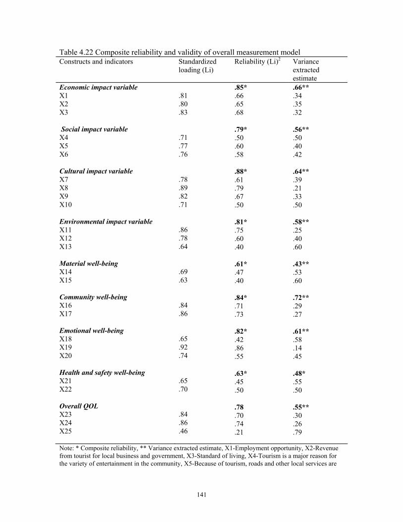
141
Table 4.22 Composite reliability and validity of overall measurement model Constructs and indicators Standardized
loading (Li) Reliability (Li)2 Variance
extracted estimate
Economic impact variable X1 X2 X3 Social impact variable X4 X5 X6 Cultural impact variable X7 X8 X9 X10 Environmental impact variable X11 X12 X13 Material well-being X14 X15 Community well-being X16 X17 Emotional well-being X18 X19 X20 Health and safety well-being X21 X22 Overall QOL X23 X24 X25
.81 .80 .83 .71 .77 .76 .78 .89 .82 .71 .86 .78 .64 .69 .63 .84 .86 .65 .92 .74 .65 .70 .84 .86 .46
.85*
.66
.65
.68 .79* .50 .60 .58 .88* .61 .79 .67 .50 .81* .75 .60 .40 .61* .47 .40 .84* .71 .73 .82* .42 .86 .55 .63* .45 .50 .78 .70 .74 .21
.66**
.34
.35
.32 .56** .50 .40 .42 .64** .39 .21 .33 .50 .58** .25 .40 .60 .43** .53 .60 .72** .29 .27 .61** .58 .14 .45 .48* .55 .50 .55** .30 .26 .79
Note: * Composite reliability, ** Variance extracted estimate, X1-Employment opportunity, X2-Revenue from tourist for local business and government, X3-Standard of living, X4-Tourism is a major reason for the variety of entertainment in the community, X5-Because of tourism, roads and other local services are
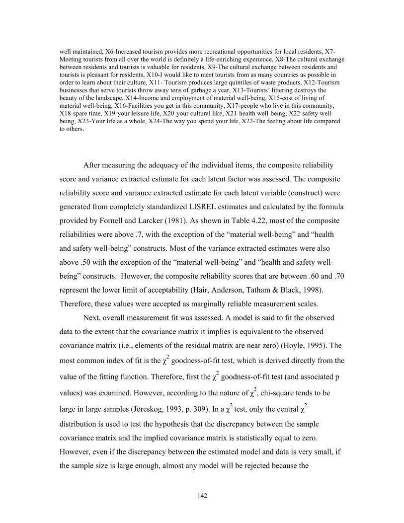
142
well maintained, X6-Increased tourism provides more recreational opportunities for local residents, X7-Meeting tourists from all over the world is definitely a life-enriching experience, X8-The cultural exchange between residents and tourists is valuable for residents, X9-The cultural exchange between residents and tourists is pleasant for residents, X10-I would like to meet tourists from as many countries as possible in order to learn about their culture, X11- Tourism produces large quintiles of waste products, X12-Tourism businesses that serve tourists throw away tons of garbage a year, X13-Tourists’ littering destroys the beauty of the landscape, X14-Income and employment of material well-being, X15-cost of living of material well-being, X16-Facilities you get in this community, X17-people who live in this community, X18-spare time, X19-your leisure life, X20-your cultural like, X21-health well-being, X22-safety well-being, X23-Your life as a whole, X24-The way you spend your life, X22-The feeling about life compared to others.
After measuring the adequacy of the individual items, the composite reliability
score and variance extracted estimate for each latent factor was assessed. The composite
reliability score and variance extracted estimate for each latent variable (construct) were
generated from completely standardized LISREL estimates and calculated by the formula
provided by Fornell and Larcker (1981). As shown in Table 4.22, most of the composite
reliabilities were above .7, with the exception of the “material well-being” and “health
and safety well-being” constructs. Most of the variance extracted estimates were also
above .50 with the exception of the “material well-being” and “health and safety well-
being” constructs. However, the composite reliability scores that are between .60 and .70
represent the lower limit of acceptability (Hair, Anderson, Tatham & Black, 1998).
Therefore, these values were accepted as marginally reliable measurement scales.
Next, overall measurement fit was assessed. A model is said to fit the observed
data to the extent that the covariance matrix it implies is equivalent to the observed
covariance matrix (i.e., elements of the residual matrix are near zero) (Hoyle, 1995). The
most common index of fit is the χ2 goodness-of-fit test, which is derived directly from the
value of the fitting function. Therefore, first the χ2 goodness-of-fit test (and associated p
values) was examined. However, according to the nature of χ2, chi-square tends to be
large in large samples (Jöreskog, 1993, p. 309). In a χ2 test, only the central χ2
distribution is used to test the hypothesis that the discrepancy between the sample
covariance matrix and the implied covariance matrix is statistically equal to zero.
However, even if the discrepancy between the estimated model and data is very small, if
the sample size is large enough, almost any model will be rejected because the

143
discrepancy is not statistically equal to zero due to the excess power of the large sample
size. In other words, the researcher is not likely to know everything about the data. In
addition, the a χ2 test offers only a dichotomous decision strategy implied by a statistical
decision rule and can not be used to quantify the degree of fit along a continuum with
some pre-specified boundary. In this case, the sample size was 321 and the χ2 value for
the saturated model was 452.23 (df 239, P=0.0). The critical N (CN) indicates that if the
sample size was 203, the χ2 goodness-of-fit test would result in a lower χ2 value, and it
would be insignificant, indicating an acceptable fit.
4.4.2.2. Fit indices
According to the problems associated with the χ2 (and associated p values),
various different types of fit indices were selected to measure the fit of the tested model
based on the recommendations of several researchers from a number of different
disciplines. These selected fit indices are absolute and incremental fit indexes. In
addition, the residuals are evaluated.
GFI, AGFI, and PGFI Indices
An absolute fit index directly assesses how well an a priori model reproduces the
sample data. It compares the hypothesized model with no model at all. However, an
implicit or explicit comparison may be made to a saturated model that reproduces the
exact observed covariance matrix. As a result, this type of fit index is analogous to R by
comparing the goodness of fit to a component that is similar to a sum of squares (Hu &
Bentler, 1995). Three absolute goodness-of-fit indices are reported in this study: the
goodness of fit (GFI), the adjusted goodness of fit (AGFI), and the parsimony goodness
of fit index (PGFI)
The GFI is a measure of the relative amount of variance and covariance in sample
data that is jointly explained by sample data (Jöreskog & Sorbom, 1989). The problem
with GFI is that it does not take into account the number of degrees of freedom in the
specified model. On the other hand, AGFI adjusts for the number of degrees of freedom
in the specified model. AGFI also addresses the issue of parsimony by incorporating a

144
penalty for the inclusion of additional parameters. Based on the GFI and AGFI values
reported in Table 4.23 (0.90 and 0.86, respectively), it is concluded that the proposed
measurement model fits the sample data marginally well.
Table 4.23 Fit indices the proposed measurement model (N=321)
Fit Index Value Chi-square with 239 degrees of freedom 452.23 (p=0.0) Goodness-of-fit Index (GFI) 0.90 Adjusted Goodness-of-fit Index (AGFI) 0.86 Parsimony Goodness-of-fit Index (PGFI) 0.66 Normed Fit Index (NFI) 0.88 Non- Normed Fit Index (NNFI) 0.92 Parsimony Normed Fit Index (PNFI) 0.70 Comparative Fit Index (CFI) 0.94 Increment Fit Index (IFI) 0.94 Relative Fit Index (RFI) 0.85 Critical N 202.68 Root Mean Square Residual (RMR) 0.047 Standized Root Mean Square Residual (SRMR) 0.047 Root Mean Square Error of Approximation (RMSEA) 0.053
Parsimony goodness of fit (PGFI) addresses the issues of parsimony in SEM. It
takes into account the complexity (i.e., the number of estimated parameters) of the
proposed model in the assessment of overall model fit. The threshold level (value) of
parsimony-based indices is lower than the threshold level of normed indices of fit
(Mulaik et al, 1989). Mulaik et al. (1989) suggest that goodness-of-fit indices in the range
of .90 accompanied by parsimonious-fit-index in the range of .50, are not unexpected. In
the light of Mulaik et al.’s suggestion, the PGFI value of the hypothesized measurement
model (.71) presented in Table 4.23 seems to be consistent with the previous fit statistics.
NFI, NNFI, PNFI, CFI, and IFI
An incremental fit index compares the target model with a baseline model in
order to measure the proportionate improvement fit. The baseline model is usually a more
restricted model than the hypothesized model. Typically, the independence or null model
is used as the baseline model because in the independence or null model all observed

145
variables are uncorrelated, and that makes it the most restricted model. Five incremental
goodness-of-fit indices are reported in the study: the Normed Fit Index (NFI), the Non-
Normed Fit Index (NNFI), the Parsimony Normed Fit Index (PNFI), the Comparative Fit
Index (CFI), and the Incremental Fit Index (IFI).
The NFI is an index of the fit between a saturated model and a null model (i.e., a
restricted model against which other less-restricted models are compared in a nested
sequence of models, Bentler & Bonett, 1980). The problem with NFI is that it does not
take into account the sample size. NFI is not a good indicator for evaluating model fit
when sample size is small because studies show that NFI has a tendency to underestimate
fit in small samples (Hu & Bentler, 1995). The value of NFI ranges from zero to 1.00
with a value >.90 indicating an acceptable fit to the data (Bentler, 1992). As shown in
Table 4.23 the NFI (0.88) was a little bit lower than the previously reported goodness-of-
fit indices in suggesting the proposed measurement model represented an adequate fit to
the data.
The NNFI takes the complexity of the model into account in the comparison of
the hypothesized model with the independence model. Since the NNFI is not normed, its
value can extend beyond the range of zero to 1.00. However, the NNFI has been found to
be unaffected by sample size (Hu & Bentler, 1995). As shown in Table 4.23, the NNFI
(0.92) indicated that the proposed measurement model represented an adequate fit to the
data.
The PNFI addresses the issue of parsimony by taking the complexity of the model
into account in its assessment of goodness-of-fit. The PNFI adjusts for the number of free
parameters in the model; it also controls for the fact that better fit can be indicated by the
other indices simply by freeing more parameters in the model (Mulaik et al., 1989). The
PNFI is calculated by multiplying the NFI with the parsimony ratio (Byrne, 1989). Like
PGFI, the PNFI usually has lower values than the threshold level generally perceived as
acceptable for other normed indices of fit. Therefore, the PNFI (.70) indicates a good fit
of the proposed measurement model to the data.
The CFI is the revised version of the NFI. Unlike NFI, it takes the sample into
account in the comparison of the hypothesized model with the independence model
(Bentler, 1990). In addition, unlike GFI, the CFI does not panelize for the
146
parsimoniousness of a model (Bentler, 1990). Given the differences in parsimony of a
priori (theoretical) models and respecified models, the CFI can ensure that conclusions
were not biased in favor of more saturated model. Values of CFI range from zero to one
with a value >.95 indicating an acceptable fit to the data (Bentler, 1992). As shown in
Table 4.23 the CFI (.94) indicated that the proposed model represented an adequate fit to
the data.
The IFI addresses the issues of parsimony and sample size that are known to be
associated with NFI. Like all the other normed fit indices, values of IFI range from zero
to one with a value>.95 indicating an acceptable fit to the data. As shown in Table 4.23
the IFI (.94) suggested that the proposed measurement model represented an adequate fit
to the data.
The last goodness-of-fit statistic reported in the study is the Hoelter’s (1983)
Critical N (CN). CN addresses the issue of sample size rather than the model fit. The CN
statistic estimates the sample size that would make the obtained chi-squire statistically
significant (Jöreskog & Sorbom, 1993). A cut-off of 200 or greater is suggested as an
indication of adequate model fit for the critical N statistic (Bollen, 1989). As shown in
Table 4.23, the CN value for the proposed model was 202.68, which the χ2 would be
significant.
Evaluation of Residuals
The Root Mean Square Residual (RMR) is a measure of the average of the fitted
residuals and can only be interpreted in relation to the sizes of the observed variances and
covariance in sample data (Jöreskog & Sorbom, 1993). It represents the average residual
value derived from the fitting of the variance-covariance matrix for the proposed model
to the variance-covariance of the sample data (Byrne, 1989). This measure works best if
all of the observed variables are standardized. It is also a good idea to report the
standardized RMR (SRMR) if the data are not standardized. The SRMR represents the
average value across all standardized residuals, and ranges from zero to one. In a well-
fitting model, the value of the SRMR should be close to .05 or less (Bryne 1989). The
value of the RMR and SRMR (.047 for both) shown in Table 4.23 represents the average

147
discrepancy between the sample observed and proposed variance-covariance matrices
and indicates a well fitting model.
Root Mean Square Error of Approximation (RMSEA) attempts to correct for the
tendency of the chi-square statistic to reject any specified model with a sufficiently large
sample. Similar to RMSR, the RMSEA is the discrepancy per degree of freedom. It
differs from the RMSR, however, in that the discrepancy is measured in terms of the
population, not just the sample used for estimation. The value is representative of the
goodness-of-fit that could be expected if the model were estimated in the population, not
just the sample drawn for the estimation. Values ranging from .05 to .08 are deemed
acceptable. The value of the RMSEA (.053) shown in Table 4.23 represents the proposed
model is acceptable.
4.4.2.3 Discriminality validity
Discriminality validity addresses the concept that “dissimilar constructs should
differ” (Burns & Bush 1995, p. 275). Applying this concept to the study at hand, this
means that the indicators used to measure the different constructs in the proposed model
should yield different results. To ensure that the constructs are not measuring the same
concept or ideas, the discriminality validity was assessed for each construct by examining
the constructs in sets of two. For instance, the economic impact of tourism was tested
against the social impact of tourism (in order to establish that these two constructs were
not measuring the same thing). Separately, the social impact of tourism was tested against
culture impact of tourism, and so forth until every possible pair of constructs was tested.
The discriminant validity tests were performed by constructing the estimated
correlation parameter between each pair of constructs to 1.0. The χ2 value was generated
for the constrained model (i.e., the “fixed” model), where the correlation parameter was
set to 1.0, indicating that the correlation between the two constructs is perfect, that is,
they are measuring exactly the same thing. Similarly, the χ2 value was generated for the
unconstrained model (i.e., the free model), where the correlation parameter was not
manipulated, but rather, the actual correlation value was calculated. A χ2 difference test
was performed on the two models. A significantly lower value χ2 value for the “free”
model demonstrates that discriminant validity has been achieved (Bagozzi & Phillips,
148
1982). Table 4.24 indicates that all of the constructs possess discriminant validity. A
closer examination of the table reveals that many of the model’s constructs are correlated.
Correlation coefficients range between +1 and –1. Most experts consider correlation
coefficients between +1 and +0.8 or –1 and –0.8 to be highly correlated; between +0.8
and +0.6 or between –0.8 and –0.6 to be moderately correlated; between +0.6 and +0.4 or
between –0.6 and –0.4 to have a weak correlation; between +0.4 and +0.2 or between –
0.4 and –0.2 to posses very weak or low correlation; and between +0.2 and –0.2 to
exhibit little or no correlation (Burns & Bush, 1995).
Most of the relationships in the proposed model show promise that they are
correlated (having already established statistical significance). For instance, the
correlation between the economic impact of tourism construct and the cultural impact of
tourism construct (i.e., 1-3) falls in the moderately correlated category (.70) whereas the
correlation between the economic impact of tourism construct and the material well-
being construct (i.e., 1-5) shows some correlation with coefficient of 0.39. It is important
to keep in mind that as the discriminant validity tests are being conducted, the indirect
and direct paths are not defined, but rather the relationships are being examined two by
two, so the correlations of the relationships during the discriminality validity testing will
most probably differ greatly from the correlations generated from the run of the actual
model. Nonetheless, having some indication of correlation at this level is a good sign that
relationships do exist among the model’s variables, although all possess discriminant
validity except the correlations between economic impact and environmental impact, and
social impact and environmental impact.
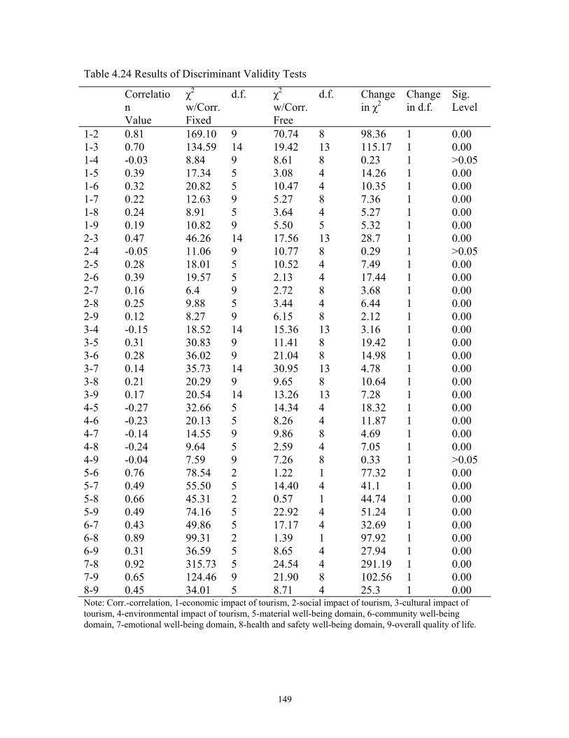
149
Table 4.24 Results of Discriminant Validity Tests
Correlation Value
χ2
w/Corr. Fixed
d.f. χ2
w/Corr. Free
d.f. Change in χ2
Change in d.f.
Sig. Level
1-2 0.81 169.10 9 70.74 8 98.36 1 0.00 1-3 0.70 134.59 14 19.42 13 115.17 1 0.00 1-4 -0.03 8.84 9 8.61 8 0.23 1 >0.05 1-5 0.39 17.34 5 3.08 4 14.26 1 0.00 1-6 0.32 20.82 5 10.47 4 10.35 1 0.00 1-7 0.22 12.63 9 5.27 8 7.36 1 0.00 1-8 0.24 8.91 5 3.64 4 5.27 1 0.00 1-9 0.19 10.82 9 5.50 5 5.32 1 0.00 2-3 0.47 46.26 14 17.56 13 28.7 1 0.00 2-4 -0.05 11.06 9 10.77 8 0.29 1 >0.05 2-5 0.28 18.01 5 10.52 4 7.49 1 0.00 2-6 0.39 19.57 5 2.13 4 17.44 1 0.00 2-7 0.16 6.4 9 2.72 8 3.68 1 0.00 2-8 0.25 9.88 5 3.44 4 6.44 1 0.00 2-9 0.12 8.27 9 6.15 8 2.12 1 0.00 3-4 -0.15 18.52 14 15.36 13 3.16 1 0.00 3-5 0.31 30.83 9 11.41 8 19.42 1 0.00 3-6 0.28 36.02 9 21.04 8 14.98 1 0.00 3-7 0.14 35.73 14 30.95 13 4.78 1 0.00 3-8 0.21 20.29 9 9.65 8 10.64 1 0.00 3-9 0.17 20.54 14 13.26 13 7.28 1 0.00 4-5 -0.27 32.66 5 14.34 4 18.32 1 0.00 4-6 -0.23 20.13 5 8.26 4 11.87 1 0.00 4-7 -0.14 14.55 9 9.86 8 4.69 1 0.00 4-8 -0.24 9.64 5 2.59 4 7.05 1 0.00 4-9 -0.04 7.59 9 7.26 8 0.33 1 >0.05 5-6 0.76 78.54 2 1.22 1 77.32 1 0.00 5-7 0.49 55.50 5 14.40 4 41.1 1 0.00 5-8 0.66 45.31 2 0.57 1 44.74 1 0.00 5-9 0.49 74.16 5 22.92 4 51.24 1 0.00 6-7 0.43 49.86 5 17.17 4 32.69 1 0.00 6-8 0.89 99.31 2 1.39 1 97.92 1 0.00 6-9 0.31 36.59 5 8.65 4 27.94 1 0.00 7-8 0.92 315.73 5 24.54 4 291.19 1 0.00 7-9 0.65 124.46 9 21.90 8 102.56 1 0.00 8-9 0.45 34.01 5 8.71 4 25.3 1 0.00 Note: Corr.-correlation, 1-economic impact of tourism, 2-social impact of tourism, 3-cultural impact of tourism, 4-environmental impact of tourism, 5-material well-being domain, 6-community well-being domain, 7-emotional well-being domain, 8-health and safety well-being domain, 9-overall quality of life.
150
4.4.2.4 Convergent validity
Convergent validity is overlaps between alternative measures that are intended to
measure the same construct but that have different sources of undesired variation (Judd,
Smith, & Kidder, 1991). In other words, if several observed indicators are used to
measure a theoretical construct (i.e., latent variable), those observed indicators should
share a good deal of variance (converge together). However, too much overlap could
indicate that discriminant validity is violated. Since the evidence presented an earlier
indication that discriminant validity has been achieved in this study, this is not a concern
at this point.
In estimating convergent validity for structural equation modeling studies,
examining the standardized confirmatory factor analysis (CFA) parameters’ estimated
pattern coefficient is one method often used (Marsh & Grayson, 1995). Convergent
validity can be assessed from the measurement model by determining whether each
indicator’s estimated pattern coefficient on its posited underlying construct factor is
significant (Anderson & Gerbing, 1988). Statistically significant large factor loadings
indicate convergent validity. That is, if the values in the off diagonal are large,
convergent validity is achieved.
As shown in Table 4.21, all of the estimated pattern coefficients on their posited
underlying construct factors were significant at 0.05 significant levels (i.e., each had a t-
value >±1.96). In fact, the smallest t-value was 7.88. Therefore, convergent validity was
achieved for all the variables in the study.
4.4.2.5 Testing the proposed model and hypotheses
The primary purpose of this study is to examine the effects of tourism impact on
residents’ quality of life in the community. More specifically, the intention is to
investigate: (1) the effect of tourism impact on the quality of life of the residents in the
community, (2) the effects of tourism impact on a particular life domain, and (3) the
effects of particular life domain on the quality of life of residents in the community.
151
Previous chapters have described and explained the logic behind the basic
theoretical model and hypotheses guiding the current study. Structural equation modeling
(i.e., LISREL 8) was used to test the goodness-of-fit of the proposed model.
Structural equation modeling is a comprehensive statistical approach to testing
hypotheses about relationships among observed and latent variables. Structural equation
modeling, resulting from an evaluation of multi-equation modeling, developed
principally in econometrics; it merged with the principles of measurement from
psychology and sociology. Structural equation modeling has emerged as an integral tool
in both managerial and academic research (Austin & Calderon, 1996).
Structural equation modeling is a multivariate statistical technique that takes a
confirmatory (i.e., hypothesis testing) approach to the multivariate analysis of a structural
theory. The most obvious difference between structural equation modeling and other
techniques is the use of separate relationships for each of a set of dependent latent
variables. Structural equation modeling estimates a series of separate, but interdependent,
multiple regression equations simultaneously by specifying the causal relationship
proposed based on the hypothesized structural model. The structural model defines the
pattern of relations among the constructs and is typically identified in schematic diagrams
by the presence of interrelated ellipses, each of which represents a hypothetical construct
(or factor). First, in this hypothesized structural model, the relationships among the
constructs are specified. Then, the hypothesized structural model is tested statistically in
a simultaneous analysis of the entire system of variables to determine the extent to which
it is consistent with the data.
Figure 4.1 presents the hypothesized tourism impact on the quality of life model
that is assessed. The model proposes that overall quality of life is influenced by the
tourism impact dimensions and particular life domains; the model also suggests that
tourism impact dimensions influence the particular life domains. The details of each
construct were discussed, and the validity and reliability of measurement scales were
confirmed earlier. In this section, the proposed structural model for phase I is assessed.
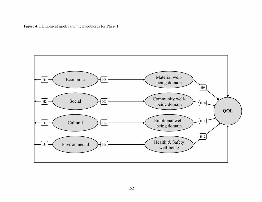
152
Figure 4.1. Empirical model and the hypotheses for Phase I
Emotional well-being domain
Economic Material well-being domain
Social
Cultural
Environmental
Community well-being domain
Health & Safety well-being
H5
H6
H7
H8
H9
H10
H11
H12
H1
H2
H3
H4
QOL

153
The final approach to model assessment is to compare the proposed model with a
series of competing models, which act as alternative explanations to the proposed model.
In this way, the proposed model can be determined, regardless of overall fit, to be
acceptable unless other similarly formulated model can achieve a higher level of fit. This
step is particularly important when the chi-square statistic indicates no significant
difference in overall model fit, because there may be better-fitting model, even in the case
of no significant differences. For the purpose of this, and as Anderson and Gerbing
(1988) recommended a series of five nested structural models to compare, five alternative
models are proposed. The first model was a saturated structural sub-model (Ms), which
can be defined as one all parameters relating the construct to one another are estimated.
This model is formally equivalent to a confirmatory measurement model. Obviously, for
the second model, a null structural sub-model (Mn), was defined as one in which all
parameters relating the constructs to one another are fixed at zero. A third structural sub-
model (Mt) represented the proposed theoretical model. Finally, the structural sub-model
Mc and Mu were represented, respectively; the next most likely constrained and
unconstrained alternatives from a theoretical perspective model of interest. That is, in
Mc, four more parameter (four direct effects from tourism impact dimensions to quality
of life) constrained in Mt, where as in Mu, two more parameter unconstrained in Mt (a
direct effects path from environmental tourism impacts to material well-being domain
and a direct effect from the material well-being domain to community well-being
domain) were estimated. Given their definitions, this set of five structural sub-models
was nested in a sequence such that Mn<Mc<Mt<Mu<Ms. Table 4.25 compares the five
models on all three types of fit measures such as absolute fit measures, increment fit
measures, and parsimonious fit measures.
Before all five-nested model were tested, the possibility that any structural model
that would have acceptable goodness of fit existed was assessed as recommended by
Anderson and Gerbing (1988). To assess whether any structural model has acceptable
goodness-of-fit, a pseudo chi-square test was utilized (Bentler & Bonett, 1980). In a
pseudo chi-square test, a pseudo chi-square statistic is constructed from the chi-square
value for the saturated model (Ms) (the smallest value possible for any structural model)
with the degrees of freedom for the null structural sub-model (Mn) (the largest number of
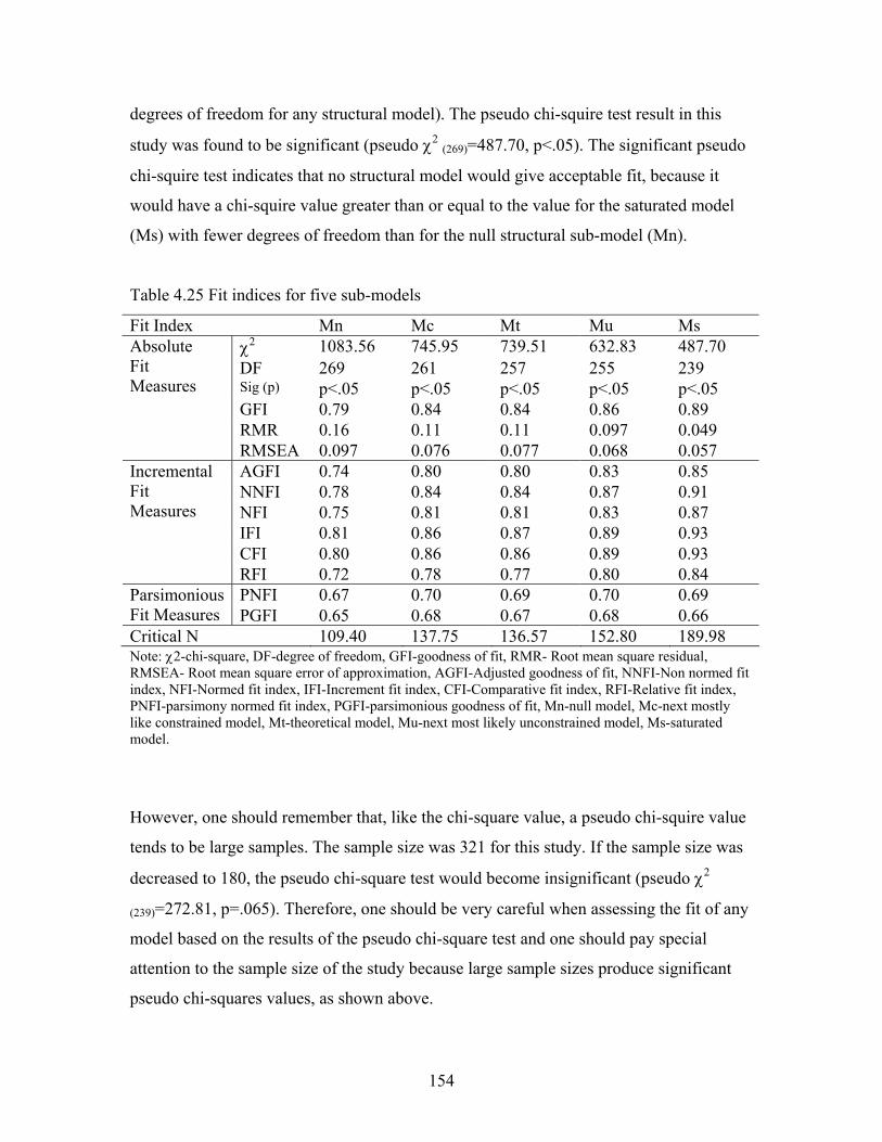
154
degrees of freedom for any structural model). The pseudo chi-squire test result in this
study was found to be significant (pseudo χ2 (269)=487.70, p<.05). The significant pseudo
chi-squire test indicates that no structural model would give acceptable fit, because it
would have a chi-squire value greater than or equal to the value for the saturated model
(Ms) with fewer degrees of freedom than for the null structural sub-model (Mn).
Table 4.25 Fit indices for five sub-models
Fit Index Mn Mc Mt Mu Ms χ2 1083.56 745.95 739.51 632.83 487.70 DF 269 261 257 255 239 Sig (p) p<.05 p<.05 p<.05 p<.05 p<.05 GFI 0.79 0.84 0.84 0.86 0.89 RMR 0.16 0.11 0.11 0.097 0.049
Absolute Fit Measures
RMSEA 0.097 0.076 0.077 0.068 0.057 AGFI 0.74 0.80 0.80 0.83 0.85 NNFI 0.78 0.84 0.84 0.87 0.91 NFI 0.75 0.81 0.81 0.83 0.87 IFI 0.81 0.86 0.87 0.89 0.93 CFI 0.80 0.86 0.86 0.89 0.93
Incremental Fit Measures
RFI 0.72 0.78 0.77 0.80 0.84 PNFI 0.67 0.70 0.69 0.70 0.69 Parsimonious
Fit Measures PGFI 0.65 0.68 0.67 0.68 0.66 Critical N 109.40 137.75 136.57 152.80 189.98 Note: χ2-chi-square, DF-degree of freedom, GFI-goodness of fit, RMR- Root mean square residual, RMSEA- Root mean square error of approximation, AGFI-Adjusted goodness of fit, NNFI-Non normed fit index, NFI-Normed fit index, IFI-Increment fit index, CFI-Comparative fit index, RFI-Relative fit index, PNFI-parsimony normed fit index, PGFI-parsimonious goodness of fit, Mn-null model, Mc-next mostly like constrained model, Mt-theoretical model, Mu-next most likely unconstrained model, Ms-saturated model.
However, one should remember that, like the chi-square value, a pseudo chi-squire value
tends to be large samples. The sample size was 321 for this study. If the sample size was
decreased to 180, the pseudo chi-square test would become insignificant (pseudo χ2
(239)=272.81, p=.065). Therefore, one should be very careful when assessing the fit of any
model based on the results of the pseudo chi-square test and one should pay special
attention to the sample size of the study because large sample sizes produce significant
pseudo chi-squares values, as shown above.
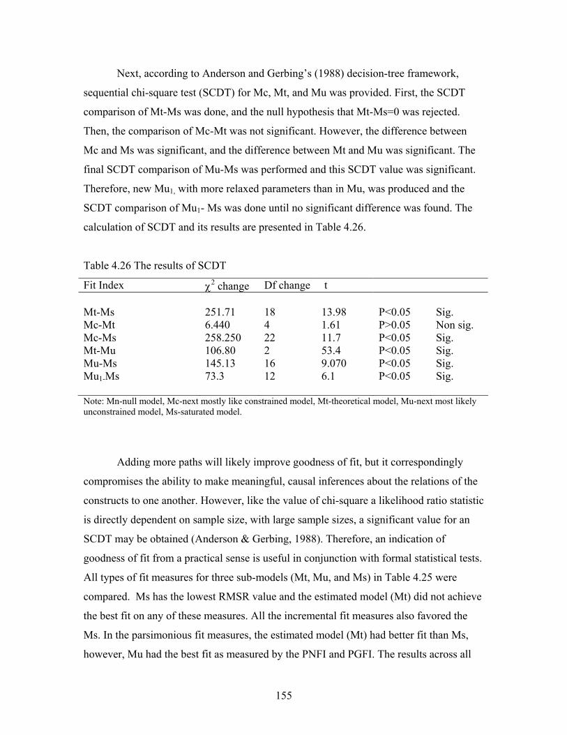
155
Next, according to Anderson and Gerbing’s (1988) decision-tree framework,
sequential chi-square test (SCDT) for Mc, Mt, and Mu was provided. First, the SCDT
comparison of Mt-Ms was done, and the null hypothesis that Mt-Ms=0 was rejected.
Then, the comparison of Mc-Mt was not significant. However, the difference between
Mc and Ms was significant, and the difference between Mt and Mu was significant. The
final SCDT comparison of Mu-Ms was performed and this SCDT value was significant.
Therefore, new Mu1, with more relaxed parameters than in Mu, was produced and the
SCDT comparison of Mu1- Ms was done until no significant difference was found. The
calculation of SCDT and its results are presented in Table 4.26.
Table 4.26 The results of SCDT
Fit Index χ2 change Df change t Mt-Ms
251.71
18
13.98
P<0.05
Sig.
Mc-Mt 6.440 4 1.61 P>0.05 Non sig. Mc-Ms 258.250 22 11.7 P<0.05 Sig. Mt-Mu 106.80 2 53.4 P<0.05 Sig. Mu-Ms 145.13 16 9.070 P<0.05 Sig. Mu1-Ms 73.3 12 6.1 P<0.05 Sig. Note: Mn-null model, Mc-next mostly like constrained model, Mt-theoretical model, Mu-next most likely unconstrained model, Ms-saturated model.
Adding more paths will likely improve goodness of fit, but it correspondingly
compromises the ability to make meaningful, causal inferences about the relations of the
constructs to one another. However, like the value of chi-square a likelihood ratio statistic
is directly dependent on sample size, with large sample sizes, a significant value for an
SCDT may be obtained (Anderson & Gerbing, 1988). Therefore, an indication of
goodness of fit from a practical sense is useful in conjunction with formal statistical tests.
All types of fit measures for three sub-models (Mt, Mu, and Ms) in Table 4.25 were
compared. Ms has the lowest RMSR value and the estimated model (Mt) did not achieve
the best fit on any of these measures. All the incremental fit measures also favored the
Ms. In the parsimonious fit measures, the estimated model (Mt) had better fit than Ms,
however, Mu had the best fit as measured by the PNFI and PGFI. The results across all
156
three types of measures showed mixed results, sometimes favoring the Ms or Mu. Thus,
although the fit of the proposed model did not exceed the recommended guidelines in
many instances, the proposed model was accepted with a reservation until additional
constructs can be added, measures refined, or causal relationship respecified.
4.4.2.5.1. Testing the hypothesized structural model
Figure 4.2 presents the hypothesized tourism impact on quality of life model that
is assessed. A close examination of the Figure 4.2 reveals the structural part of the model
has nine constructs (latent variables) and four of these latent variables are the
independent variables and the other five are dependent variables. As shown in Figure 4.2,
the independent measurement model comprises three observed indicator variables (X1,
X2 and X3) for economic impact construct, three observed indicators (X4, X5, and X6)
for social impact of tourism construct, four observed indicators (X7, X8, X9 and X10) for
cultural impact of tourism construct, and three observed indicators (X11, X12, and X13)
for environmental impact of tourism construct along with their related measurement error
terms. The dependent variables are material well-being (Y1 and Y2), community well-
being (Y3 and Y4), emotional well-being (Y5, Y6 and Y7), health and safety well-being
(Y8 and Y9), and overall quality of life (Y10, Y11, and Y12) constructs. The dependent
measurement model comprised of 12 observed indicator variables (Y1-Y12)
accompanied by their associated error terms.
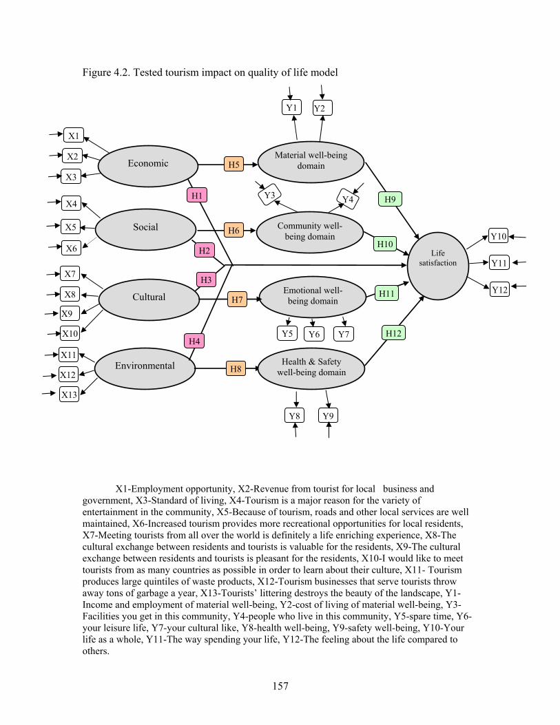
157
Figure 4.2. Tested tourism impact on quality of life model X1-Employment opportunity, X2-Revenue from tourist for local business and government, X3-Standard of living, X4-Tourism is a major reason for the variety of entertainment in the community, X5-Because of tourism, roads and other local services are well maintained, X6-Increased tourism provides more recreational opportunities for local residents, X7-Meeting tourists from all over the world is definitely a life enriching experience, X8-The cultural exchange between residents and tourists is valuable for the residents, X9-The cultural exchange between residents and tourists is pleasant for the residents, X10-I would like to meet tourists from as many countries as possible in order to learn about their culture, X11- Tourism produces large quintiles of waste products, X12-Tourism businesses that serve tourists throw away tons of garbage a year, X13-Tourists’ littering destroys the beauty of the landscape, Y1-Income and employment of material well-being, Y2-cost of living of material well-being, Y3-Facilities you get in this community, Y4-people who live in this community, Y5-spare time, Y6-your leisure life, Y7-your cultural like, Y8-health well-being, Y9-safety well-being, Y10-Your life as a whole, Y11-The way spending your life, Y12-The feeling about the life compared to others.
Emotional well-being domain
Economic Material well-being
domain
Social
Cultural
Environmental
Community well-being domain
Health & Safety well-being domain
Life satisfaction
H9
H10
H11
H12
H5
H6
H7
H8
X6
X5
X4
Y9 Y8
Y7 Y6 Y5
Y4 Y3
Y2 Y1
X3
X2
X1
Y12
Y11
Y10
X13
X12
X11
X10
X9
X8
X7
H1
H2
H3
H4

158
In structural equation modeling, two types of matrices are examined: a Gamma
matrix and a Beta matrix. The Gamma matrix specifies the regression coefficients that
link dependent and independent constructs while the beta matrix specifies the regression
coefficients that link dependent constructs. A close examination of the structural paths of
the hypothesized model reveals that there are eight parameters to be estimated in the
Gamma matrix, and four parameters to be estimated in the Beta matrix. Each of these
matrices represents one of the hypotheses proposed earlier. Both Gamma and Beta
matrices are presented in Table 4.27. Subscripts numbers in Table 4.27 represents the
hypothesized paths for both the Gamma (γ) and the Beta (β) matrices. For example, while
γ11 in the Gamma matrix represents hypothesis 1 (H1) (residents’ life satisfaction in
general is a positive function of their perceptions of the benefits of the economic impact
of tourism), β51 in the Beta matrix represents hypothesis 9 (residents’ life satisfaction in
general is a positive function of material well-being domain). Table 4.27 Pattern of estimated parameters in the Gamma and Beta matrices
Gamma Matrix Material
well-being Community well-being
Emotional well-being
Health and safety well-being
Overall QOL
Economic impact
γ11 0 0 0 γ15
Social impact 0 γ22 0 0 γ25 Cultural impact 0 0 γ33 0 γ35 Environmental impact
0 0 0 γ44 γ45
Beta Matrix Material well-being
0 0 0 0 0
Community well-being
0 0 0 0 0
Emotional well-being
0 0 0 0 0
Health and safety well-being
0 0 0 0 0
Overall QOL β51 β52 β53 β54 0 Note: γ=Gamma; β=Beta First subscript number represents the row number and the second subscript number represents the column number.

159
The results were first examined for nonsensical or theoretically inconsistent
estimates. The three common offending estimates are negative error variance,
standardized coefficients exceeding or very close to 1.0, or very large error variances.
The examination of the standardized results reveals no instances of any of these
problems. Table 4.28 presents the selected goodness-of-fit statistics for the hypothesized
tourism impacts on quality of life model. The χ2 value with 257 degrees of freedom is
739.51 (p<0.05). This indicates that model fit is not good. Because the sensitivity of this
measure is not overly affected by the sample size of 321, the use of the χ2 test can
provide evidence that a significant difference exists. However, it should be also noted
that the chi-squire test becomes more sensitive as the number of indicators rises.
Table 4.28 Fit-indices the proposed theoretical model (N=321)
Fit Index Value Chi-square with 257 degrees of freedom 739.51 (p<.05) Goodness-of-fit Index (GFI) 0.84 Adjusted Goodness-of-fit Index (AGFI) 0.80 Parsimony Goodness-of-fit Index (PGFI) 0.67 Normed Fit Index (NFI) 0.81 Non- Normed Fit Index (NNFI) 0.84 Parsimony Normed Fit Index (PNFI) 0.69 Comparative Fit Index (CFI) 0.86 Increment Fit Index (IFI) 0.87 Relative Fit Index (RFI) 0.77 Critical N 136.57 Root Mean Square Residual (RMR) 0.11 Standized Root Mean Square Residual (SRMR) 0.11 Root Mean Square Error of Approximation (RMSEA) 0.077
Therefore, it is more beneficial to check a number of other measures. The GFI value of
0.84 is at a marginal acceptance level (Hair et al., 1998), as is the RMSR value of 0.11,
which is not acceptable. The RMSEA has a value of 0.077, which falls in the acceptable
range of 0.08 or less. A few of the absolute fit measures indicated that the model is
marginally acceptable at best, but most of the absolute fit measures indicated the model is
hardly acceptable. In addition to overall measures of fit, the AGFI , NFI, NNFI, CFI, and

160
IFI all fall slightly below the desired threshold of 0.95. However, all increment fit
measures exceeded .80, therefore, only marginal support for this model was provided.
The estimated standardized path coefficients for the hypothesized model are
presented in Table 4. 29. As shown in Table 4. 29, not all of the hypothesized paths in the
model were significant at a 0.05 probability levels. The estimated standardized path
coefficients for the path from economic impact of tourism to material well-being domain
is 0.37 (p<0.01), from social impact of tourism to community well-being domain is 0.40
(p<0.01), from cultural impact of tourism to emotional well-being domain is 0.17
(p<0.01), and from environment impact of tourism to health and safety well-being is -
0.24 (p<0.01). The estimated standardized path coefficients from economic impact of
tourism to overall QOL (–0.12), from social impact of tourism to QOL (0.01), from the
cultural impact of tourism to QOL (0.10), and from environmental impact of tourism to
QOL (0.11) are not significant at the 0.05 probability levels.
Table 4.29 Estimated standardized coefficients for the hypothesized model
Material well-being
Community well-being
Emotional well-being
Health and safety well-being
Overall QOL
Economic impact
0.37** (4.60)
-0.12 (-0.71)
Social impact 0.40** (4.85)
0.01 (0.07)
Cultural impact 0.17** (2.66)
0.10 (1.04)
Environmental impact
-0.24** (-2.63)
0.11 (1.76)
Material well-being
Community well-being
Emotional well-being
Health and safety well-being
Overall QOL 0.36** (4.35)
-0.08 (-1.17)
0.58** (7.85)
0.12 (1.55)
R2 0.13 0.16 0.03 0.06 0.49 Note: t-value in parentheses, **significant at 0.01 probability level.
161
4.4.2.5.2. Analysis of the Hypotheses
The hypothesized theoretical model and proposed hypotheses tested using
LISREL 8 indicated that half of the proposed paths were significant. Therefore, the
results only supported five of the proposed twelve main hypotheses. This section of the
chapter provides a detailed discussion analysis of the hypotheses.
Hypothesis 1: Residents’ life satisfaction in general is a positive function of their
perceptions of the benefits of the economic impact of tourism.
Hypothesis 2: Residents’ life satisfaction in general is a positive function of their
perceptions of the benefits of the social impact of tourism.
Hypothesis 3: Residents’ life satisfaction in general is a positive function of their
perceptions of the benefits of the cultural impact of tourism.
Hypothesis 4: Residents’ life satisfaction in general is a positive function of their
perceptions of the benefits of the environmental impact of tourism.
In hypotheses one to four, there were postulated that there are direct positive
relationships between various dimensions of tourism impacts and overall life satisfaction.
However, the result of the LISREL analysis did not support these hypotheses. Altogether
(four tourism dimensions), the tourism impacts significantly explained 3.6% of the total
variance of overall life satisfaction. However, individually, the residents’ perceptions of
the benefits of the economic impact of tourism (H1: gamma=-0.12, p>0.05), the benefits
of the social impact of tourism (H2: gamma= 0.01, p>0.05), the benefits of the cultural
impact of tourism (H3: gamma= 0.10, p>0.05), and the benefits of the environmental
impact of tourism (H4: gamma= 0.11, p>0.05) were not significantly related to their
overall life satisfaction.
The result reported here is consistent with previous research findings. Even
though there was no study to test the direct effects from the dimension of the tourism
162
impact to overall life satisfaction of the residents in the community, in terms of tourism
sense, because once a community becomes destination, the lives of residents in the
community are affected by the tourism (Jurowski, 1994). The development of tourism
results in life conditions of the residents in a better or worse ways. These life conditions
make up the life domains in general. Usually, the perceptions of the tourism impact
influence these life conditions. Therefore, the satisfactions or dissatisfactions with living
condition (e.g., employments and income) influenced by the perception of the tourism
impacts spill over vertically to satisfactions of the life domains. Consequently, the
satisfaction of the particular life condition influences the overall life satisfaction of the
residents. In addition, it should be noted that even though the effect of the tourism
impacts on overall life satisfaction did not show statistical significance, some sense of
direct effects of the tourism impacts on overall life satisfaction still existed.
Hypothesis 5: Material well-being domain is a positive function of the perception of the
economic impact of tourism.
Hypothesis 9: Residents’ life satisfaction in general is a positive function of material
well-being domain.
In hypothesis five, it was postulated that residents’ perception of economic impact
of tourism influences positively their life satisfaction of the material well-being domain.
Consequently, in hypothesis nine, the material well-being domain influenced by the
economic tourism impact affects the overall quality of life of the residents. These
hypotheses were supported by LISEREL analysis. The perception of the economic impact
of tourism significantly influenced the satisfaction of the material well-being in one of
the particular life domains (gamma = 0.37, p<0.01). Then, the satisfaction of the material
well-being domain significantly influenced the satisfaction of the overall life of the
residents in the community (beta=0.36, p<0.01). Results indicate that as the residents’
perception of the benefits of the economic impacts of tourism increases, they are more
likely to have satisfaction with their life condition related to materials. Consequently, as
163
the life satisfaction in material well-being domain increases, the overall life satisfaction
of the residents will increase.
Findings of this study are consistent with findings of the previous quality of life
study. Abrams (1973) found the four domains were health, intimacy, material well being,
and productivity when he asked respondents to indicate how various domains of life are
important to them. Then Campbell, Converse, and Rodgers (1976) asked people to rate
domain importance on a five point scale, and found four domains were scored 91%, 89%,
73%, and 70% for health, intimacy, material well being, and productivity, respectively.
Flanagan (1978) and Krupinski (1980) also found that the five domains were regarded as
very important aspects of their lives by a large majority of people, and scored health,
97%; intimacy, 81%; emotional, 86%; material well being, 83%; and productivity, 78%.
Like this, the positive perception of the economic impact of tourism effects on the
satisfaction of the material well-being domain of the residents in the community, this
satisfaction of the material well being domain influenced the overall life satisfaction of
the residents. Economic impact of tourism accounted for 13% of the variance in the
satisfaction of the material well-being.
Hypothesis 6: Community well-being domain is a positive function of the perception of
social impact of tourism.
Hypothesis 10: Residents’ life satisfaction in general is a positive function of community
well-being domain.
In hypothesis six, it was postulated that residents’ perception of social impact of
tourism influences positively in their life satisfaction of the community well-being
domain. Consequently, in hypothesis ten, the community well-being domain influenced
by the social tourism impact affects the satisfaction of the overall quality of life of the
residents. Hypothesis 6 was supported by LISREL analysis. The perception of the social
impact of tourism significantly influenced the satisfaction of the community well-being
domain (gamma = 0.40, p<0.01). Result indicates that as the residents’ perception of the
164
benefits of the social impacts of tourism (because of tourism, roads and other local
services are well maintained, tourism is a major reason for the variety of entertainment in
the community, and increased tourism provides recreational opportunities for local
residents) increases, they are more likely to satisfy with their life condition related to
community. However, the satisfaction of the community well-being domain did not
significantly influence the satisfaction of the overall life of the residents in the
community (beta=-0.08, p<0.01). In addition, the result indicated that the satisfaction of
the community well being slightly influenced the overall life satisfaction in a negative
way. However, even though the 16% of the total variance of the satisfaction of the
community well being was accounted by social impact of tourism, the satisfaction of the
community well being domain did not influence the overall life satisfaction,.
In that sense, its result was consistant with the findings of the previous quality of
life studies. Cummins, McCabe, Romeo, and Gullone (1994) have provided both
empirical and theoretical arguments for use of community well being as one of important
seven domains. And also, Cummins (1996) reviewed 32 studies and found the
community well being as one of the majorities supported life satisfaction domains. Also,
in the perception of tourism impact studies, it was a little bit consistent with the previous
studies. In Perdue, Long and Kang’s (1999) study about residents’ perception of
community safety, community involvement, local political influence, changes in job
opportunities, social environment, and community congestion influenced their quality of
life in the community, their findings showed that the key community characteristics
affecting residents’ QOL were community safety, social environment, and community
involvement. In that sense, the satisfaction of the community well being comes not only
community service like maintaining good road condition or increasing entertainment, but
also community safety or social environment which is spilled over from the other life
domains.

165
Hypothesis 7: Emotional well-being domain is a positive function of the perception of
cultural impact of tourism.
Hypothesis 11: Residents’ life satisfaction in general is a positive function of emotional
well-being domain.
A hypothesis 7 proposes that as residents’ perception of cultural impact of
tourism increases their emotional life satisfaction are likely to increase. And
consequently, hypothesis 11 proposes that the emotional well being affected by the
perception of the cultural impact of tourism is like to influence the overall life
satisfaction. Both of the hypotheses were supported by LISREL analysis. The positive
perception of the cultural impact of tourism, such as the cultural exchange between
residents and tourists is valuable and pleasant for the residents in the community,
influenced statistically significantly the satisfaction of the emotional well being like the
satisfaction of the leisure life or cultural life (gamma=0.17, p<0.05). Consequently, the
emotional well-being affected by the cultural impact of the tourism was related
significantly to the overall life satisfaction (beta=0.58, p<0.01). However, the cultural
impact of tourism explained only 3% of the total variance of the satisfaction of the
emotional well-being. The results indicate that as the residents’ positive perception of the
cultural impact of tourism increases, their emotional satisfaction is likely to increases.
These finding are also supported by previous research. McCabe, Romeo, and Gullone
(1994) and Cummins (1996) have provided that emotional well being was the one of the
major life satisfaction domains.
Hypothesis 8: Health and Safety well-being domain is a positive function of the
perception of environmental impact of tourism.
Hypothesis 12: Residents’ life satisfaction in general is a positive function of health and
safety well-being domain.
166
In hypothesis 8, it was postulated that as the residents’ positive perception of the
environmental impact of tourism increases the satisfaction of the health and safety well
being is likely to increases, and consequently, in hypothesis 12, it was postulated that as
the satisfaction of the health and safety well being affected by the perception of the
environmental impact of the tourism increases the overall life satisfaction is likely to
increase. Only hypothesis 8 was supported by LISREL, but the hypothesis 12 was not
supported. In hypothesis 8, the residents in the community significantly perceived the
negative environmental impact of the tourism, and its result, the negative perception of
the environmental of the tourism, such as tourism produce large quantities of waste
products or tourists’ littering destroys the beauty of the landscape affected in negative
ways of the satisfaction of the health and safety well being (gamma=-0.24 p<0.05). The
result indicated that as the negative perception of the environmental impact of the tourism
increases, the overall life satisfaction decreases. The environmental impact of tourism
explained 6% of the total variance of the satisfaction of the health and safety well being.
However, even though the satisfaction of the health and safety well being did not affect
statistically significant the overall life satisfaction (beta=0.12 p>0.05, t=1.55), the results
of LISREL was close to be significant with t-value, 1.55. The results indicate that means
that as the satisfaction of the health and safety well being increases, the overall life
satisfaction is likely to increase. Altogether, tourism impact dimension and particular life
domains (material, community, emotional, and health and safety well-being) explained
49% of the total variance of the overall life satisfaction.
4.4.2.6 Testing of the moderating effect
This stage of data analysis deals with the moderating effects of tourism
development stages on the relationship between the impact of tourism and the particular
life domains. The basic premise of these moderating effects is that responses to variations
in the satisfaction of particular life domains depend on the level of tourism development.
The study used the hierarchical multiple regression/correlation (HMRC) to examine these
moderating effects.

167
The following procedures were articulated by Cohen and Cohen (1983). Each
dependent variable (i.e., the particular well-being domain such as the material well-being,
community well-being, emotional well-being, and health and safety well-being) was
regressed on an independent variable (i.e., tourism impact dimensions such as economic,
social, cultural and environmental impact of tourism) and a moderator, the tourism
development stage recoded as dummy variables. Hypotheses 13 to 16 were examined
using the Hierarchical MRC procedure in analyzing the data. For the purpose of
examining that there is existing gabs between the moderating effects of the tourism
development stages pre-selected and the moderating effects of residents’ perceptions of
the tourism development stages in their community, hypothesis 13 to 16 were tested
twice using tourism development stages pre-selected as a moderating variable for the first
time and using residents’ perceived tourism development stages for the second time. The
section below describes its procedure and hypothesis testing results.
Hypothesis 13: The relationship between economic impact of tourism and material well-
being is strongest in relation to the beginning and growth stages of the tourism
development cycle and weakest in relation to the maturity and decline stages.
For a sample of 321 responses, Y was the satisfaction of the material well being,
the quantitative independent variables were the perception of the economic impact of
tourism (represented by X1) and four groups were given different tourism development
stages. By recoding the nominal scale (tourism development stages) to dummy variable
coding, the decline stage was set as the reference group, with D1, D2, D3 (X2, X3, X4)
coded as 0,0,0; beginning stage was coded, 1,0,0; growth stage was coded 0,1,0, maturity
stage was coded 0,0,1. Next, interaction variables were formed by multiplying the
independent variable of economic impact by three dummy variables of tourism
development stages, resulting in the following three independent variables.
X5=X1X2=eco*D1, X6=X1X3=eco*D2, X7=X1X4=eco*D3.
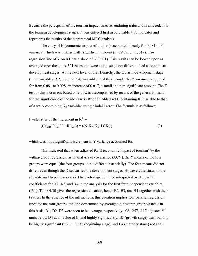
168
Because the perception of the tourism impact assesses enduring traits and is antecedent to
the tourism development stages, it was entered first as X1. Table 4.30 indicates and
represents the results of the hierarchical MRC analysis.
The entry of E (economic impact of tourism) accounted linearly for 0.081 of Y
variance, which was a statistically significant amount (F=28.03, df=1, 319). The
regression line of Y on X1 has a slope of .28(=B1). This results can be looked upon as
averaged over the entire 321 cases that were at this stage not differentiated as to tourism
development stages. At the next level of the Hierarchy, the tourism development stage
(three variables; X2, X3, and X4) was added and this brought the Y variance accounted
for from 0.081 to 0.098, an increase of 0.017, a small and non-significant amount. The F
test of this increment based on 2 df was accomplished by means of the general formula
for the significance of the increase in R2 of an added set B containing KB variable to that
of a set A containing KA variables using Model I error. The formula is as follows;
F –statistics of the increment in R2 =
((R2AB
- R2A)/ (1- R2
AB )) * ((N-KA-KB-1)/ KB ) (3)
which was not a significant increment in Y variance accounted for.
This indicated that when adjusted for E (economic impact of tourism) by the
within-group regression, as in analysis of covariance (ACV), the Y means of the four
groups were equal (the four groups do not differ substantially). The four means did not
differ, even though the D set carried the development stages. However, the status of the
separate null hypotheses carried by each stage could be interpreted by the partial
coefficients for X2, X3, and X4 in the analysis for the first four independent variables
(IVs). Table 4.30 gives the regression equation, hence B2, B3, and B4 together with their
t ratios. In the absence of the interactions, this equation implies four parallel regression
lines for the four groups, the line determined by averaged out within group values. On
this basis, D1, D2, D3 were seen to be average, respectively, .08, .257, .117 adjusted Y
units below D4 at all value of E, and highly significantly. B3 (growth stage) was found to
be highly significant (t=2.399), B2 (beginning stage) and B4 (maturity stage) not at all
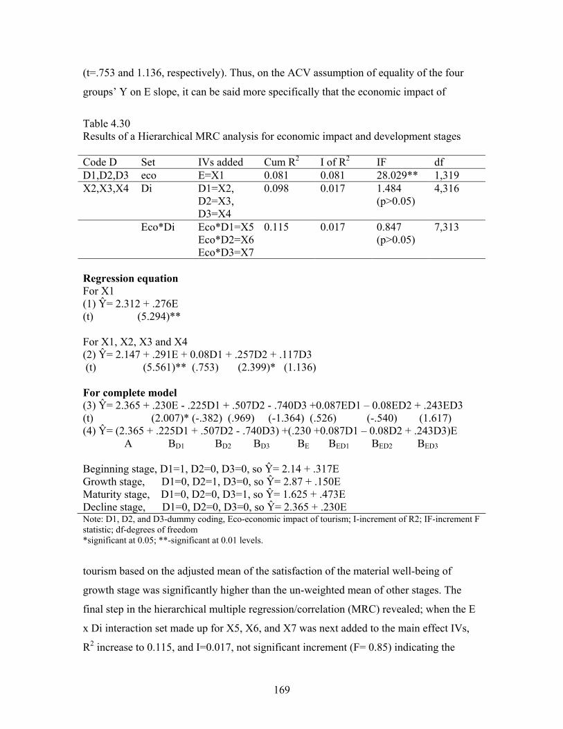
169
(t=.753 and 1.136, respectively). Thus, on the ACV assumption of equality of the four
groups’ Y on E slope, it can be said more specifically that the economic impact of
Table 4.30 Results of a Hierarchical MRC analysis for economic impact and development stages Code D Set IVs added Cum R2 I of R2 IF df D1,D2,D3 eco E=X1 0.081 0.081 28.029** 1,319 X2,X3,X4 Di D1=X2,
D2=X3, D3=X4
0.098 0.017 1.484 (p>0.05)
4,316
Eco*Di Eco*D1=X5 Eco*D2=X6 Eco*D3=X7
0.115 0.017 0.847 (p>0.05)
7,313
Regression equation For X1 (1) Ŷ= 2.312 + .276E (t) (5.294)** For X1, X2, X3 and X4 (2) Ŷ= 2.147 + .291E + 0.08D1 + .257D2 + .117D3 (t) (5.561)** (.753) (2.399)* (1.136) For complete model (3) Ŷ= 2.365 + .230E - .225D1 + .507D2 - .740D3 +0.087ED1 – 0.08ED2 + .243ED3 (t) (2.007)* (-.382) (.969) (-1.364) (.526) (-.540) (1.617) (4) Ŷ= (2.365 + .225D1 + .507D2 - .740D3) +(.230 +0.087D1 – 0.08D2 + .243D3)E A BD1 BD2 BD3 BE BED1 BED2 BED3 Beginning stage, D1=1, D2=0, D3=0, so Ŷ= 2.14 + .317E Growth stage, D1=0, D2=1, D3=0, so Ŷ= 2.87 + .150E Maturity stage, D1=0, D2=0, D3=1, so Ŷ= 1.625 + .473E Decline stage, D1=0, D2=0, D3=0, so Ŷ= 2.365 + .230E� Note: D1, D2, and D3-dummy coding, Eco-economic impact of tourism; I-increment of R2; IF-increment F statistic; df-degrees of freedom *significant at 0.05; **-significant at 0.01 levels.
tourism based on the adjusted mean of the satisfaction of the material well-being of
growth stage was significantly higher than the un-weighted mean of other stages. The
final step in the hierarchical multiple regression/correlation (MRC) revealed; when the E
x Di interaction set made up for X5, X6, and X7 was next added to the main effect IVs,
R2 increase to 0.115, and I=0.017, not significant increment (F= 0.85) indicating the

170
homogeneity of the slopes of best fitting lines between groups, and hence, validation of
the covariance model. Even though there was no slope difference among four groups, the
Y means were adjusted on the basis of a common slope. Although the insignificance of
the interaction variables render the Analysis of Covariance (ACV) analysis valid, it
would be a serious error to conclude from this that the research is un-interpretable. The
MRC analysis provides a rich yield of information from the data that may materially
increase the investigator’s insight into the phenomena under study. To illustrate this, the
complete regression equation with the composite coefficient for each stage was restated
in Table 30 from equation (3). The first is a constant, and the second is a function of E
(economic impact of tourism).
From this, it can be seen how each regression coefficient and the Y intercept A of
the full equation can be interpreted in terms of the properties of the regression of, and
differences in regressions between, the separate groups, according to the interpretation
specific to dummy variables coded nominal scales.
1. A and BE are the constants defining the regression for the reference group (in here
decline stage). Because BE is significant, the reference group’s Y on E regression differs
significantly from that of a horizontal straight line.
2. BED1 is the amount by which the linear coefficient (slope) for D1 (Beginning stage) is
larger than that for the reference group and BD1 is the amount by which the Y intercept of
D1 is larger than that for the reference group. Neither its slope nor Y intercept differs
significantly from those for the reference group.
3. Similarly, BED2 and BD2 carry differences of the reference group (decline stage) from
growth stage in regard to slope and intercept. Also, BED3 and BD3 carry differences of the
reference group (decline stage) from maturity stage in regard to slope and intercept.
However, none of them is significant, indicating evidence that the shape of growth
stages’ population regression line does not differ from that of a reference group.
A graphic plot of the best fitting linear regression equation for each of the four
groups was prepared by substituting a few values for economic impact of tourism in each

171
of four equations at the bottom Table 4.30. The results of this procedure are presented in
Figure 4.3.
Figure 4.3 Best fitting line of the relationship between the economic impact of tourism and material well-being for each stage from the full model
0
1
2
3
4
5
E=1 E=2 E=3 E=4 E=5
Economic impact of tourism
Satis
fact
ion
of th
e m
ater
ial w
ell b
eing
B=2.14 + .317E
G=2.87 + .150E
M=1.625 + .473E
D=2.365 + .230E
The statement made above about the best fitting line of Y on E for decline stage
(control group) and differences between the latter and each of the other three groups can
be visualized directly from the lines in the figure. Even though the statistical analysis did
not indicate markedly different relationships between level of the perception of the
economic impact of tourism and the satisfaction of the material well-being, in practical
sense, an interpretation can be an increase of one point of economic impact of tourism is
associated with an average increase of 0.473 points in the satisfaction of the material
well-being for the residents in tourism maturity development stage. This is three times as
great as that for the residents in the growth stage.
Comparison with residents’ perceived development stages
To find out any difference if it exists between the moderating effects of
development stages selected by secondary indicators and the moderating effects of
residents’ actual perceived development stages, the same procedure was done by using
the perceived development stage variable. For a sample of 286 responses, Y is the
satisfaction of the material well being, the quantitative independent variables was the
same as the perception of the economic impact of tourism (represented by X1) and four
groups were given perceived tourism development stages. By recoding the perceived
development stages to dummy variable coding, the decline stage was again set as the
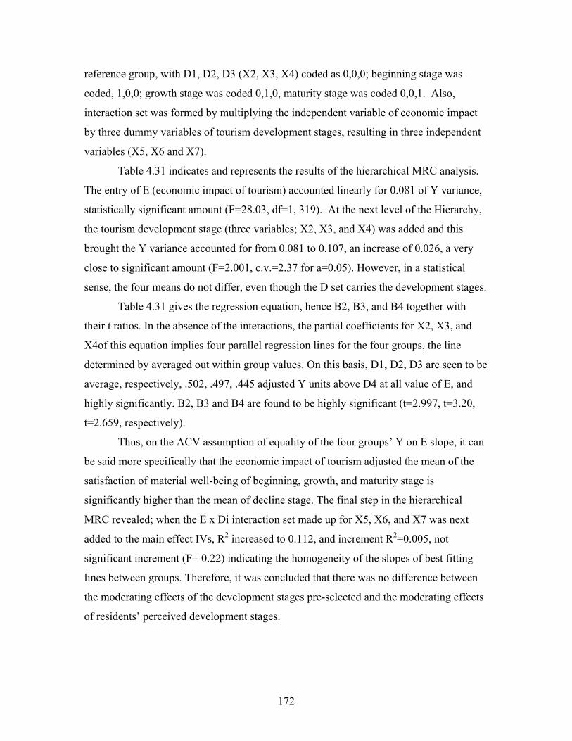
172
reference group, with D1, D2, D3 (X2, X3, X4) coded as 0,0,0; beginning stage was
coded, 1,0,0; growth stage was coded 0,1,0, maturity stage was coded 0,0,1. Also,
interaction set was formed by multiplying the independent variable of economic impact
by three dummy variables of tourism development stages, resulting in three independent
variables (X5, X6 and X7).
Table 4.31 indicates and represents the results of the hierarchical MRC analysis.
The entry of E (economic impact of tourism) accounted linearly for 0.081 of Y variance,
statistically significant amount (F=28.03, df=1, 319). At the next level of the Hierarchy,
the tourism development stage (three variables; X2, X3, and X4) was added and this
brought the Y variance accounted for from 0.081 to 0.107, an increase of 0.026, a very
close to significant amount (F=2.001, c.v.=2.37 for a=0.05). However, in a statistical
sense, the four means do not differ, even though the D set carries the development stages.
Table 4.31 gives the regression equation, hence B2, B3, and B4 together with
their t ratios. In the absence of the interactions, the partial coefficients for X2, X3, and
X4of this equation implies four parallel regression lines for the four groups, the line
determined by averaged out within group values. On this basis, D1, D2, D3 are seen to be
average, respectively, .502, .497, .445 adjusted Y units above D4 at all value of E, and
highly significantly. B2, B3 and B4 are found to be highly significant (t=2.997, t=3.20,
t=2.659, respectively).
Thus, on the ACV assumption of equality of the four groups’ Y on E slope, it can
be said more specifically that the economic impact of tourism adjusted the mean of the
satisfaction of material well-being of beginning, growth, and maturity stage is
significantly higher than the mean of decline stage. The final step in the hierarchical
MRC revealed; when the E x Di interaction set made up for X5, X6, and X7 was next
added to the main effect IVs, R2 increased to 0.112, and increment R2=0.005, not
significant increment (F= 0.22) indicating the homogeneity of the slopes of best fitting
lines between groups. Therefore, it was concluded that there was no difference between
the moderating effects of the development stages pre-selected and the moderating effects
of residents’ perceived development stages.
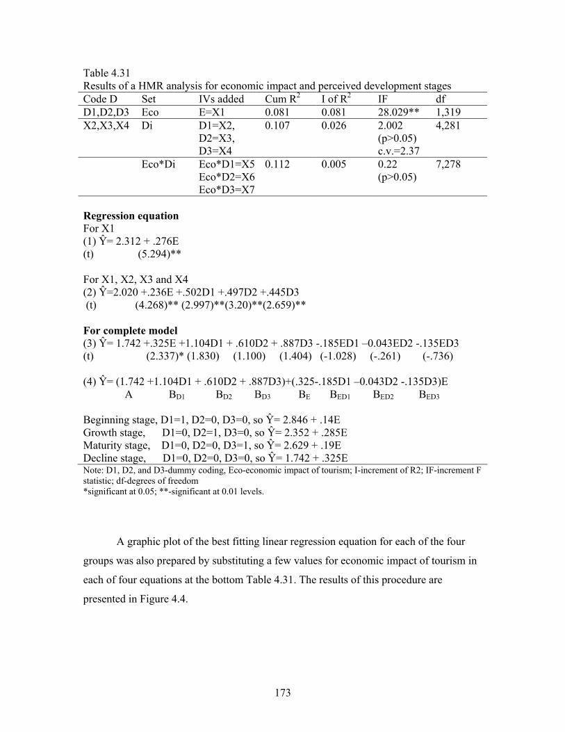
173
Table 4.31 Results of a HMR analysis for economic impact and perceived development stages Code D Set IVs added Cum R2 I of R2 IF df D1,D2,D3 Eco E=X1 0.081 0.081 28.029** 1,319 X2,X3,X4 Di D1=X2,
D2=X3, D3=X4
0.107 0.026 2.002 (p>0.05) c.v.=2.37
4,281
Eco*Di Eco*D1=X5 Eco*D2=X6 Eco*D3=X7
0.112 0.005 0.22 (p>0.05)
7,278
Regression equation For X1 (1) Ŷ= 2.312 + .276E (t) (5.294)** For X1, X2, X3 and X4 (2) Ŷ=2.020 +.236E +.502D1 +.497D2 +.445D3 (t) (4.268)** (2.997)**(3.20)**(2.659)** For complete model (3) Ŷ= 1.742 +.325E +1.104D1 + .610D2 + .887D3 -.185ED1 –0.043ED2 -.135ED3 (t) (2.337)* (1.830) (1.100) (1.404) (-1.028) (-.261) (-.736) (4) Ŷ= (1.742 +1.104D1 + .610D2 + .887D3)+(.325-.185D1 –0.043D2 -.135D3)E A BD1 BD2 BD3 BE BED1 BED2 BED3 Beginning stage, D1=1, D2=0, D3=0, so Ŷ= 2.846 + .14E Growth stage, D1=0, D2=1, D3=0, so Ŷ= 2.352 + .285E Maturity stage, D1=0, D2=0, D3=1, so Ŷ= 2.629 + .19E Decline stage, D1=0, D2=0, D3=0, so Ŷ= 1.742 + .325E� Note: D1, D2, and D3-dummy coding, Eco-economic impact of tourism; I-increment of R2; IF-increment F statistic; df-degrees of freedom *significant at 0.05; **-significant at 0.01 levels.
A graphic plot of the best fitting linear regression equation for each of the four
groups was also prepared by substituting a few values for economic impact of tourism in
each of four equations at the bottom Table 4.31. The results of this procedure are
presented in Figure 4.4.
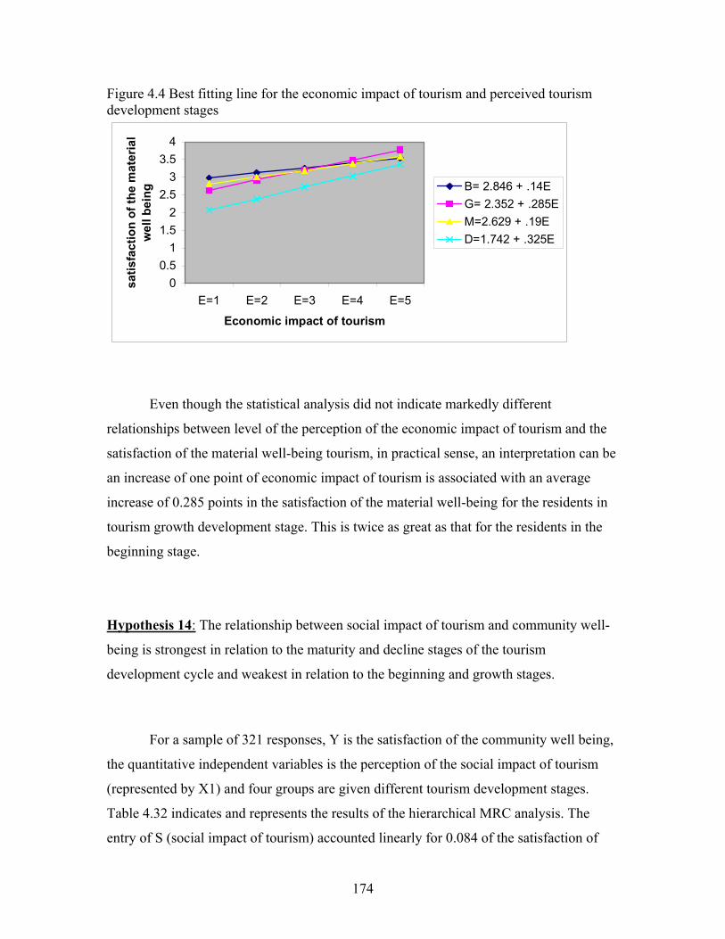
174
Figure 4.4 Best fitting line for the economic impact of tourism and perceived tourism development stages
00.5
11.5
22.5
33.5
4
E=1 E=2 E=3 E=4 E=5
Economic impact of tourism
satis
fact
ion
of th
e m
ater
ial
wel
l bei
ng B= 2.846 + .14EG= 2.352 + .285EM=2.629 + .19ED=1.742 + .325E
Even though the statistical analysis did not indicate markedly different
relationships between level of the perception of the economic impact of tourism and the
satisfaction of the material well-being tourism, in practical sense, an interpretation can be
an increase of one point of economic impact of tourism is associated with an average
increase of 0.285 points in the satisfaction of the material well-being for the residents in
tourism growth development stage. This is twice as great as that for the residents in the
beginning stage.
Hypothesis 14: The relationship between social impact of tourism and community well-
being is strongest in relation to the maturity and decline stages of the tourism
development cycle and weakest in relation to the beginning and growth stages.
For a sample of 321 responses, Y is the satisfaction of the community well being,
the quantitative independent variables is the perception of the social impact of tourism
(represented by X1) and four groups are given different tourism development stages.
Table 4.32 indicates and represents the results of the hierarchical MRC analysis. The
entry of S (social impact of tourism) accounted linearly for 0.084 of the satisfaction of
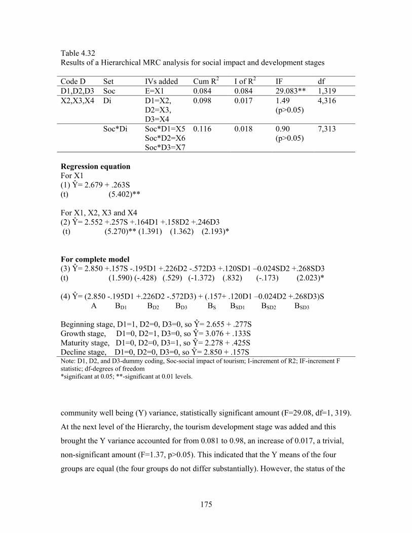
175
Table 4.32 Results of a Hierarchical MRC analysis for social impact and development stages Code D Set IVs added Cum R2 I of R2 IF df D1,D2,D3 Soc E=X1 0.084 0.084 29.083** 1,319 X2,X3,X4 Di D1=X2,
D2=X3, D3=X4
0.098 0.017 1.49 (p>0.05)
4,316
Soc*Di Soc*D1=X5 Soc*D2=X6 Soc*D3=X7
0.116 0.018 0.90 (p>0.05)
7,313
Regression equation For X1 (1) Ŷ= 2.679 + .263S (t) (5.402)** For X1, X2, X3 and X4 (2) Ŷ= 2.552 +.257S +.164D1 +.158D2 +.246D3 (t) (5.270)** (1.391) (1.362) (2.193)* For complete model (3) Ŷ= 2.850 +.157S -.195D1 +.226D2 -.572D3 +.120SD1 –0.024SD2 +.268SD3 (t) (1.590) (-.428) (.529) (-1.372) (.832) (-.173) (2.023)* (4) Ŷ= (2.850 -.195D1 +.226D2 -.572D3) + (.157+ .120D1 –0.024D2 +.268D3)S A BD1 BD2 BD3 BS BSD1 BSD2 BSD3 Beginning stage, D1=1, D2=0, D3=0, so Ŷ= 2.655 + .277S Growth stage, D1=0, D2=1, D3=0, so Ŷ= 3.076 + .133S Maturity stage, D1=0, D2=0, D3=1, so Ŷ= 2.278 + .425S Decline stage, D1=0, D2=0, D3=0, so Ŷ= 2.850 + .157S� Note: D1, D2, and D3-dummy coding, Soc-social impact of tourism; I-increment of R2; IF-increment F statistic; df-degrees of freedom *significant at 0.05; **-significant at 0.01 levels.
community well being (Y) variance, statistically significant amount (F=29.08, df=1, 319).
At the next level of the Hierarchy, the tourism development stage was added and this
brought the Y variance accounted for from 0.081 to 0.98, an increase of 0.017, a trivial,
non-significant amount (F=1.37, p>0.05). This indicated that the Y means of the four
groups are equal (the four groups do not differ substantially). However, the status of the
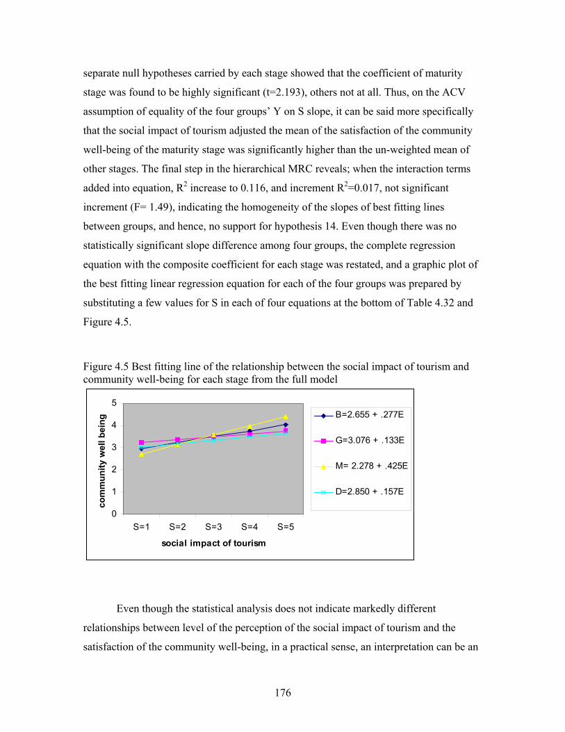
176
separate null hypotheses carried by each stage showed that the coefficient of maturity
stage was found to be highly significant (t=2.193), others not at all. Thus, on the ACV
assumption of equality of the four groups’ Y on S slope, it can be said more specifically
that the social impact of tourism adjusted the mean of the satisfaction of the community
well-being of the maturity stage was significantly higher than the un-weighted mean of
other stages. The final step in the hierarchical MRC reveals; when the interaction terms
added into equation, R2 increase to 0.116, and increment R2=0.017, not significant
increment (F= 1.49), indicating the homogeneity of the slopes of best fitting lines
between groups, and hence, no support for hypothesis 14. Even though there was no
statistically significant slope difference among four groups, the complete regression
equation with the composite coefficient for each stage was restated, and a graphic plot of
the best fitting linear regression equation for each of the four groups was prepared by
substituting a few values for S in each of four equations at the bottom of Table 4.32 and
Figure 4.5.
Figure 4.5 Best fitting line of the relationship between the social impact of tourism and community well-being for each stage from the full model
0
1
2
3
4
5
S=1 S=2 S=3 S=4 S=5
social impact of tourism
com
mun
ity w
ell b
eing
B=2.655 + .277E
G=3.076 + .133E
M= 2.278 + .425E
D=2.850 + .157E
Even though the statistical analysis does not indicate markedly different
relationships between level of the perception of the social impact of tourism and the
satisfaction of the community well-being, in a practical sense, an interpretation can be an

177
increase of one point of social impact of tourism is associated with an average increase of
0.425 points in the satisfaction of the community well-being for the residents in tourism
maturity development stage. This is three times as great as that for the residents in the
growth stage.
Comparison with the perceived development stages
To find out existing gabs between the moderating effects of development stages
selected by secondary indicators and the moderating effects of residents’ actual perceived
development stages on the relationship between social impact of tourism and community
well being, HMRC was done by using the perceived development stage variable. A
sample of 286 responses, Y is the satisfaction of the community well being, the
quantitative independent variable is the perception of the social impact of tourism
(represented by X1) and four groups are given residents’ perceived tourism development
stages. By recoding the perceived development stages to dummy variable coding, the
decline stage is again set the control group, as the reference group, with D1, D2, D3 (X2,
X3, X4) coded as 0,0,0; beginning stage is coded, 1,0,0; growth stage is coded 0,1,0,
maturity stage is coded 0,0,1. Also, interaction set was formed by multiplying the
independent variable of social impact by three dummy variables of tourism development
stages, resulting in three independent variables (X5, X6, and X7).
Table 4.33 indicates and represents the results of the hierarchical MRC analysis.
The entry of S (social impact of tourism) accounted linearly for 0.084 of Y variance,
statistically significant amount (F=29.08, df=1, 319). At the next level of the Hierarchy,
the perceived tourism development stage (three variables; X2, X3, and X4) was added
and this brought the Y variance accounted for from 0.083 to 0.115, an increase of 0.031,
to a significant increase of the amount (F=2.45, c.v.=2.37 for a=0.05).
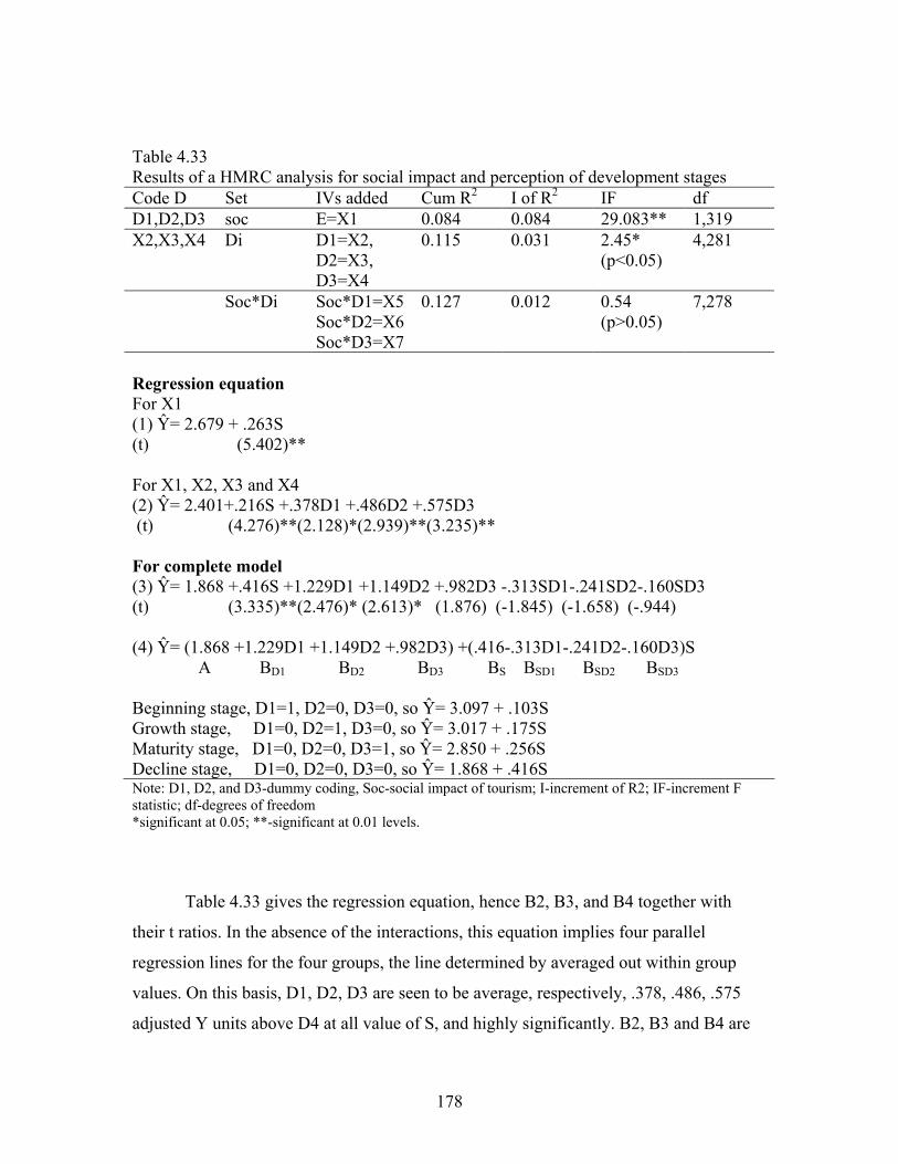
178
Table 4.33 Results of a HMRC analysis for social impact and perception of development stages Code D Set IVs added Cum R2 I of R2 IF df D1,D2,D3 soc E=X1 0.084 0.084 29.083** 1,319 X2,X3,X4 Di D1=X2,
D2=X3, D3=X4
0.115 0.031 2.45* (p<0.05)
4,281
Soc*Di Soc*D1=X5 Soc*D2=X6 Soc*D3=X7
0.127 0.012 0.54 (p>0.05)
7,278
Regression equation For X1 (1) Ŷ= 2.679 + .263S (t) (5.402)** For X1, X2, X3 and X4 (2) Ŷ= 2.401+.216S +.378D1 +.486D2 +.575D3 (t) (4.276)**(2.128)*(2.939)**(3.235)** For complete model (3) Ŷ= 1.868 +.416S +1.229D1 +1.149D2 +.982D3 -.313SD1-.241SD2-.160SD3 (t) (3.335)**(2.476)* (2.613)* (1.876) (-1.845) (-1.658) (-.944) (4) Ŷ= (1.868 +1.229D1 +1.149D2 +.982D3) +(.416-.313D1-.241D2-.160D3)S A BD1 BD2 BD3 BS BSD1 BSD2 BSD3 Beginning stage, D1=1, D2=0, D3=0, so Ŷ= 3.097 + .103S Growth stage, D1=0, D2=1, D3=0, so Ŷ= 3.017 + .175S Maturity stage, D1=0, D2=0, D3=1, so Ŷ= 2.850 + .256S Decline stage, D1=0, D2=0, D3=0, so Ŷ= 1.868 + .416S� Note: D1, D2, and D3-dummy coding, Soc-social impact of tourism; I-increment of R2; IF-increment F statistic; df-degrees of freedom *significant at 0.05; **-significant at 0.01 levels.
Table 4.33 gives the regression equation, hence B2, B3, and B4 together with
their t ratios. In the absence of the interactions, this equation implies four parallel
regression lines for the four groups, the line determined by averaged out within group
values. On this basis, D1, D2, D3 are seen to be average, respectively, .378, .486, .575
adjusted Y units above D4 at all value of S, and highly significantly. B2, B3 and B4 are
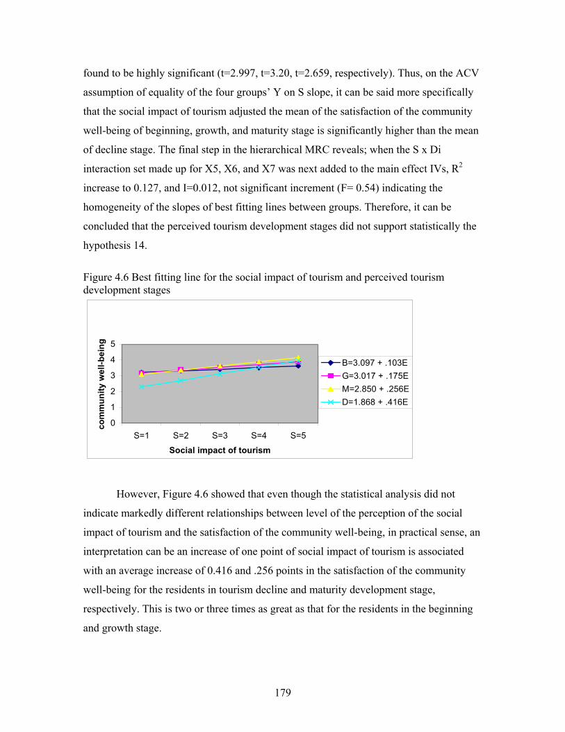
179
found to be highly significant (t=2.997, t=3.20, t=2.659, respectively). Thus, on the ACV
assumption of equality of the four groups’ Y on S slope, it can be said more specifically
that the social impact of tourism adjusted the mean of the satisfaction of the community
well-being of beginning, growth, and maturity stage is significantly higher than the mean
of decline stage. The final step in the hierarchical MRC reveals; when the S x Di
interaction set made up for X5, X6, and X7 was next added to the main effect IVs, R2
increase to 0.127, and I=0.012, not significant increment (F= 0.54) indicating the
homogeneity of the slopes of best fitting lines between groups. Therefore, it can be
concluded that the perceived tourism development stages did not support statistically the
hypothesis 14.
Figure 4.6 Best fitting line for the social impact of tourism and perceived tourism development stages
0
1
2
3
4
5
S=1 S=2 S=3 S=4 S=5
Social impact of tourism
com
mun
ity w
ell-b
eing
B=3.097 + .103EG=3.017 + .175EM=2.850 + .256ED=1.868 + .416E
However, Figure 4.6 showed that even though the statistical analysis did not
indicate markedly different relationships between level of the perception of the social
impact of tourism and the satisfaction of the community well-being, in practical sense, an
interpretation can be an increase of one point of social impact of tourism is associated
with an average increase of 0.416 and .256 points in the satisfaction of the community
well-being for the residents in tourism decline and maturity development stage,
respectively. This is two or three times as great as that for the residents in the beginning
and growth stage.
180
Hypothesis 15: The relationship between cultural impact of tourism and emotional well-
being is strongest in relation to the maturity and decline stages of the tourism
development cycle and weakest in relation to the beginning and growth stages.
For a sample of 321 responses, Y is the satisfaction of the emotional well being,
the quantitative independent variables is the perception of the cultural impact of tourism
(represented by X1) and four groups are given different tourism development stages.
Table 4.34 indicates and represents the results of the hierarchical MRC analysis. The
entry of C (cultural impact of tourism) accounted linearly for 0.023 of the satisfaction of
the emotional well being (Y) variance, statistically significant amount (F=7.39, df=1,
319). At the next level of the Hierarchy, the tourism development stage was added and
this brought the Y variance accounted for from 0.023 to 0.36, an increase of 0.013, a
trivial, non-significant amount (F=1.06, p>0.05). This indicates that the Y means of the
four groups are equal (the four groups do not differ substantially) presenting the
coefficient of each stage was not significant at all. The final step in the hierarchical MRC
revealed; when the interaction terms added into equation, R2 increase to 0.046, and
I=0.010, not significant increment (F= 0.46), indicating the homogeneity of the slopes of
best fitting lines between groups, and hence, no support for hypothesis 15. Even though
there is no statistically significant slope difference among four groups, the complete
regression equation with the composite coefficient for each stage was restated, and a
graphic plot of the best fitting linear regression equation for each of the four groups was
prepared by substituting a few values for C in each of four equations at the bottom Table
4.34. The plot of the results is presented in Figure 4.7.
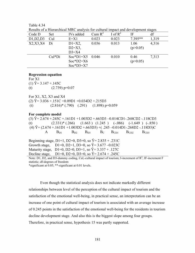
181
Table 4.34 Results of a Hierarchical MRC analysis for cultural impact and development stages Code D Set IVs added Cum R2 I of R2 IF df D1,D2,D3 Cul E=X1 0.023 0.023 7.395** 1,319 X2,X3,X4 Di D1=X2,
D2=X3, D3=X4
0.036 0.013 1.06 (p>0.05)
4,316
Cul*Di Soc*D1=X5 Soc*D2=X6 Soc*D3=X7
0.046 0.010 0.46 (p>0.05)
7,313
Regression equation For X1 (1) Ŷ= 3.147 +.145C (t) (2.739) p=0.07 For X1, X2, X3 and X4 (2) Ŷ= 3.036 +.151C +0.09D1 +0.034D2 +.215D3 (t) (2.816)* (.790) (.291) (1.898) p=0.059 For complete model (3) Ŷ= 2.674 +.245C +.161D1 +1.003D2 +.663D3 –0.014CD1-.268CD2 -.118CD3 (t) (2.331)* (.266) (1.663 ) (1.245 ) (-.086) (-1.649 ) (-.850 ) (4) Ŷ= (2.674 +.161D1 +1.003D2 +.663D3) +( .245 –0.014D1-.268D2 -.118D3)C A BD1 BD2 BD3 BC BCD1 BCD2 BCD3 Beginning stage, D1=1, D2=0, D3=0, so Ŷ= 2.835 + .231C Growth stage, D1=0, D2=1, D3=0, so Ŷ= 3.677 –0.023C Maturity stage, D1=0, D2=0, D3=1, so Ŷ= 3.337 + .127C Decline stage, D1=0, D2=0, D3=0, so Ŷ= 2.674 + .245C� Note: D1, D2, and D3-dummy coding, Cul,-cultural impact of tourism; I-increment of R2; IF-increment F statistic; df-degrees of freedom *significant at 0.05; **-significant at 0.01 levels.
Even though the statistical analysis does not indicate markedly different
relationships between level of the perception of the cultural impact of tourism and the
satisfaction of the emotional well-being, in practical sense, an interpretation can be an
increase of one point of cultural impact of tourism is associated with an average increase
of 0.245 points in the satisfaction of the emotional well-being for the residents in tourism
decline development stage. And also this is the biggest slope among four groups.
Therefore, in practical sense, hypothesis 15 was partly supported.
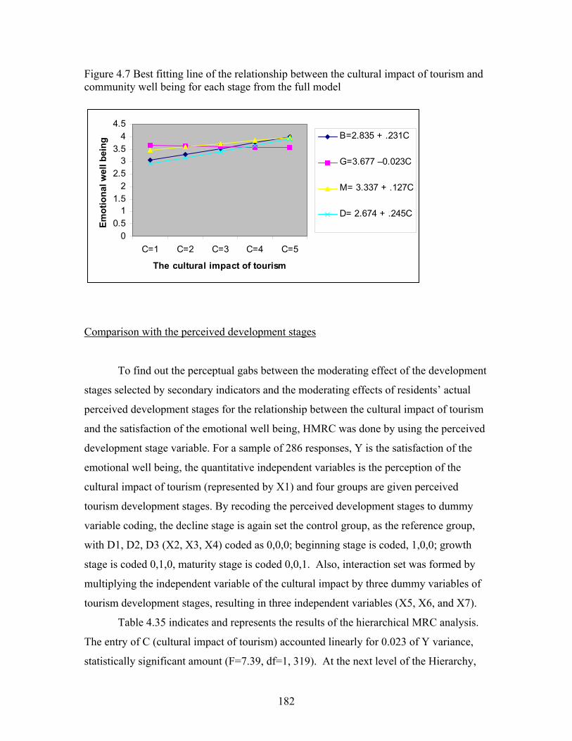
182
Figure 4.7 Best fitting line of the relationship between the cultural impact of tourism and community well being for each stage from the full model
00.5
11.5
22.5
33.5
44.5
C=1 C=2 C=3 C=4 C=5
The cultural impact of tourism
Emot
iona
l wel
l bei
ng
B=2.835 + .231C
G=3.677 –0.023C
M= 3.337 + .127C
D= 2.674 + .245C
Comparison with the perceived development stages
To find out the perceptual gabs between the moderating effect of the development
stages selected by secondary indicators and the moderating effects of residents’ actual
perceived development stages for the relationship between the cultural impact of tourism
and the satisfaction of the emotional well being, HMRC was done by using the perceived
development stage variable. For a sample of 286 responses, Y is the satisfaction of the
emotional well being, the quantitative independent variables is the perception of the
cultural impact of tourism (represented by X1) and four groups are given perceived
tourism development stages. By recoding the perceived development stages to dummy
variable coding, the decline stage is again set the control group, as the reference group,
with D1, D2, D3 (X2, X3, X4) coded as 0,0,0; beginning stage is coded, 1,0,0; growth
stage is coded 0,1,0, maturity stage is coded 0,0,1. Also, interaction set was formed by
multiplying the independent variable of the cultural impact by three dummy variables of
tourism development stages, resulting in three independent variables (X5, X6, and X7).
Table 4.35 indicates and represents the results of the hierarchical MRC analysis.
The entry of C (cultural impact of tourism) accounted linearly for 0.023 of Y variance,
statistically significant amount (F=7.39, df=1, 319). At the next level of the Hierarchy,
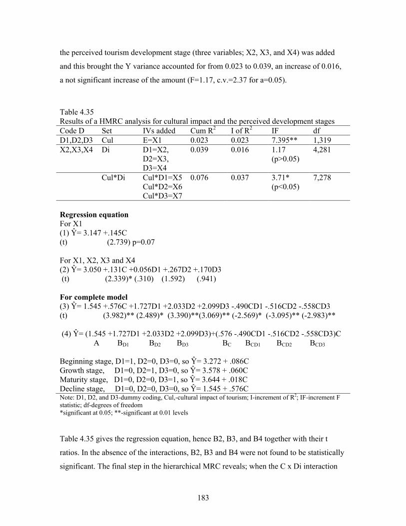
183
the perceived tourism development stage (three variables; X2, X3, and X4) was added
and this brought the Y variance accounted for from 0.023 to 0.039, an increase of 0.016,
a not significant increase of the amount (F=1.17, c.v.=2.37 for a=0.05).
Table 4.35 Results of a HMRC analysis for cultural impact and the perceived development stages Code D Set IVs added Cum R2 I of R2 IF df D1,D2,D3 Cul E=X1 0.023 0.023 7.395** 1,319 X2,X3,X4 Di D1=X2,
D2=X3, D3=X4
0.039 0.016 1.17 (p>0.05)
4,281
Cul*Di Cul*D1=X5 Cul*D2=X6 Cul*D3=X7
0.076 0.037 3.71* (p<0.05)
7,278
Regression equation For X1 (1) Ŷ= 3.147 +.145C (t) (2.739) p=0.07 For X1, X2, X3 and X4 (2) Ŷ= 3.050 +.131C +0.056D1 +.267D2 +.170D3 (t) (2.339)* (.310) (1.592) (.941) For complete model (3) Ŷ= 1.545 +.576C +1.727D1 +2.033D2 +2.099D3 -.490CD1 -.516CD2 -.558CD3 (t) (3.982)** (2.489)* (3.390)**(3.069)** (-2.569)* (-3.095)** (-2.983)** (4) Ŷ= (1.545 +1.727D1 +2.033D2 +2.099D3)+(.576 -.490CD1 -.516CD2 -.558CD3)C A BD1 BD2 BD3 BC BCD1 BCD2 BCD3 Beginning stage, D1=1, D2=0, D3=0, so Ŷ= 3.272 + .086C Growth stage, D1=0, D2=1, D3=0, so Ŷ= 3.578 + .060C Maturity stage, D1=0, D2=0, D3=1, so Ŷ= 3.644 + .018C Decline stage, D1=0, D2=0, D3=0, so Ŷ= 1.545 + .576C� Note: D1, D2, and D3-dummy coding, Cul,-cultural impact of tourism; I-increment of R2; IF-increment F statistic; df-degrees of freedom *significant at 0.05; **-significant at 0.01 levels
Table 4.35 gives the regression equation, hence B2, B3, and B4 together with their t
ratios. In the absence of the interactions, B2, B3 and B4 were not found to be statistically
significant. The final step in the hierarchical MRC reveals; when the C x Di interaction
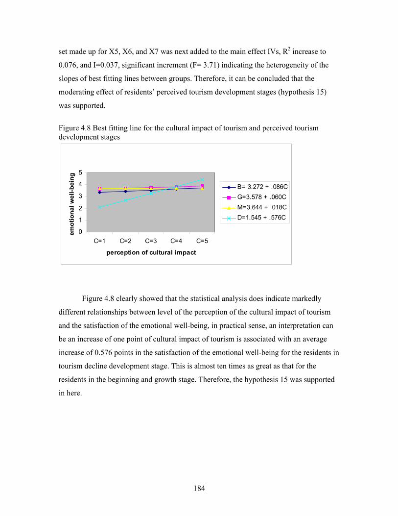
184
set made up for X5, X6, and X7 was next added to the main effect IVs, R2 increase to
0.076, and I=0.037, significant increment (F= 3.71) indicating the heterogeneity of the
slopes of best fitting lines between groups. Therefore, it can be concluded that the
moderating effect of residents’ perceived tourism development stages (hypothesis 15)
was supported.
Figure 4.8 Best fitting line for the cultural impact of tourism and perceived tourism development stages
0
1
2
3
4
5
C=1 C=2 C=3 C=4 C=5
perception of cultural impact
emot
iona
l wel
l-bei
ng
B= 3.272 + .086CG=3.578 + .060CM=3.644 + .018CD=1.545 + .576C
Figure 4.8 clearly showed that the statistical analysis does indicate markedly
different relationships between level of the perception of the cultural impact of tourism
and the satisfaction of the emotional well-being, in practical sense, an interpretation can
be an increase of one point of cultural impact of tourism is associated with an average
increase of 0.576 points in the satisfaction of the emotional well-being for the residents in
tourism decline development stage. This is almost ten times as great as that for the
residents in the beginning and growth stage. Therefore, the hypothesis 15 was supported
in here.
185
Hypothesis 16: The relationship between environmental impact of tourism and health
and safety well-being is strongest in relation to the maturity and decline stages of the
tourism development cycle and weakest in relation to the beginning and growth stages.
In sample of 321 responses, Y is the satisfaction of the health and safety well
being, the quantitative independent variables is the perception of the environmental
impact of tourism (represented by X1) and four groups are given different tourism
development stages. Table 4.36 indicates and represents the results of the hierarchical
MRC analysis. The entry of EN (environmental impact of tourism) accounted linearly for
0.023 of the satisfaction of the emotional well-being (Y) variance, statistically significant
amount (F=7.19, df=1, 319). At the next level of the Hierarchy, the tourism development
stage was added and this brought the Y variance accounted for from 0.023 to 0.091, an
increase of 0.068, a significant amount (F=5.89, p<0.01). This indicates that the Y means
of the four groups do differ substantially presenting the coefficient of each stage was
significant. In the absence of the interactions, this equation implies four parallel
regression lines for the four groups, the line determined by averaged out within group
values. On this basis, D1, D2, D3 were seen to be average, respectively, .197, .290, .504
adjusted Y units above D4 at all value of EN, and highly significantly. B3 (growth stage)
and B4 (maturity stage) were found to be highly significant (t=2.606 and t=4.731,
respectively), B2 (beginning stage) not at all (t=1.746). Thus, on the ACV assumption of
equality of the four groups’ Y on EN slope, it can be said more specifically that the
environmental impact of tourism adjusted the mean of the satisfaction of the health and
safety well-being of growth and maturity stage was significantly higher than the un-
weighted mean of other stages. The final step in the hierarchical MRC reveals; when the
interaction terms added into equation, R2 increase to 0.105, and I=0.014, not significant
increment (F= 0.70), indicating the homogeneity of the slopes of best fitting lines
between groups, and hence, no support for hypothesis 16. Even though there is no
statistically significant slope difference among four groups, the complete regression
equation with the composite coefficient for each stage was restated, and a graphic plot of
the best fitting linear regression equation for each of the four groups was visualized by
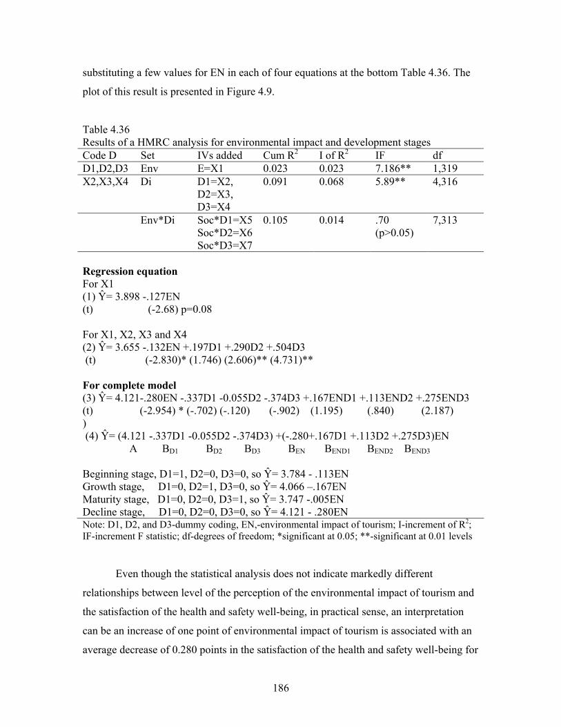
186
substituting a few values for EN in each of four equations at the bottom Table 4.36. The
plot of this result is presented in Figure 4.9.
Table 4.36 Results of a HMRC analysis for environmental impact and development stages Code D Set IVs added Cum R2 I of R2 IF df D1,D2,D3 Env E=X1 0.023 0.023 7.186** 1,319 X2,X3,X4 Di D1=X2,
D2=X3, D3=X4
0.091 0.068 5.89**
4,316
Env*Di Soc*D1=X5 Soc*D2=X6 Soc*D3=X7
0.105 0.014 .70 (p>0.05)
7,313
Regression equation For X1 (1) Ŷ= 3.898 -.127EN (t) (-2.68) p=0.08 For X1, X2, X3 and X4 (2) Ŷ= 3.655 -.132EN +.197D1 +.290D2 +.504D3 (t) (-2.830)* (1.746) (2.606)** (4.731)** For complete model (3) Ŷ= 4.121-.280EN -.337D1 -0.055D2 -.374D3 +.167END1 +.113END2 +.275END3 (t) (-2.954) * (-.702) (-.120) (-.902) (1.195) (.840) (2.187) ) (4) Ŷ= (4.121 -.337D1 -0.055D2 -.374D3) +(-.280+.167D1 +.113D2 +.275D3)EN A BD1 BD2 BD3 BEN BEND1 BEND2 BEND3 Beginning stage, D1=1, D2=0, D3=0, so Ŷ= 3.784 - .113EN Growth stage, D1=0, D2=1, D3=0, so Ŷ= 4.066 –.167EN Maturity stage, D1=0, D2=0, D3=1, so Ŷ= 3.747 -.005EN Decline stage, D1=0, D2=0, D3=0, so Ŷ= 4.121 - .280EN Note: D1, D2, and D3-dummy coding, EN,-environmental impact of tourism; I-increment of R2; IF-increment F statistic; df-degrees of freedom; *significant at 0.05; **-significant at 0.01 levels
Even though the statistical analysis does not indicate markedly different
relationships between level of the perception of the environmental impact of tourism and
the satisfaction of the health and safety well-being, in practical sense, an interpretation
can be an increase of one point of environmental impact of tourism is associated with an
average decrease of 0.280 points in the satisfaction of the health and safety well-being for
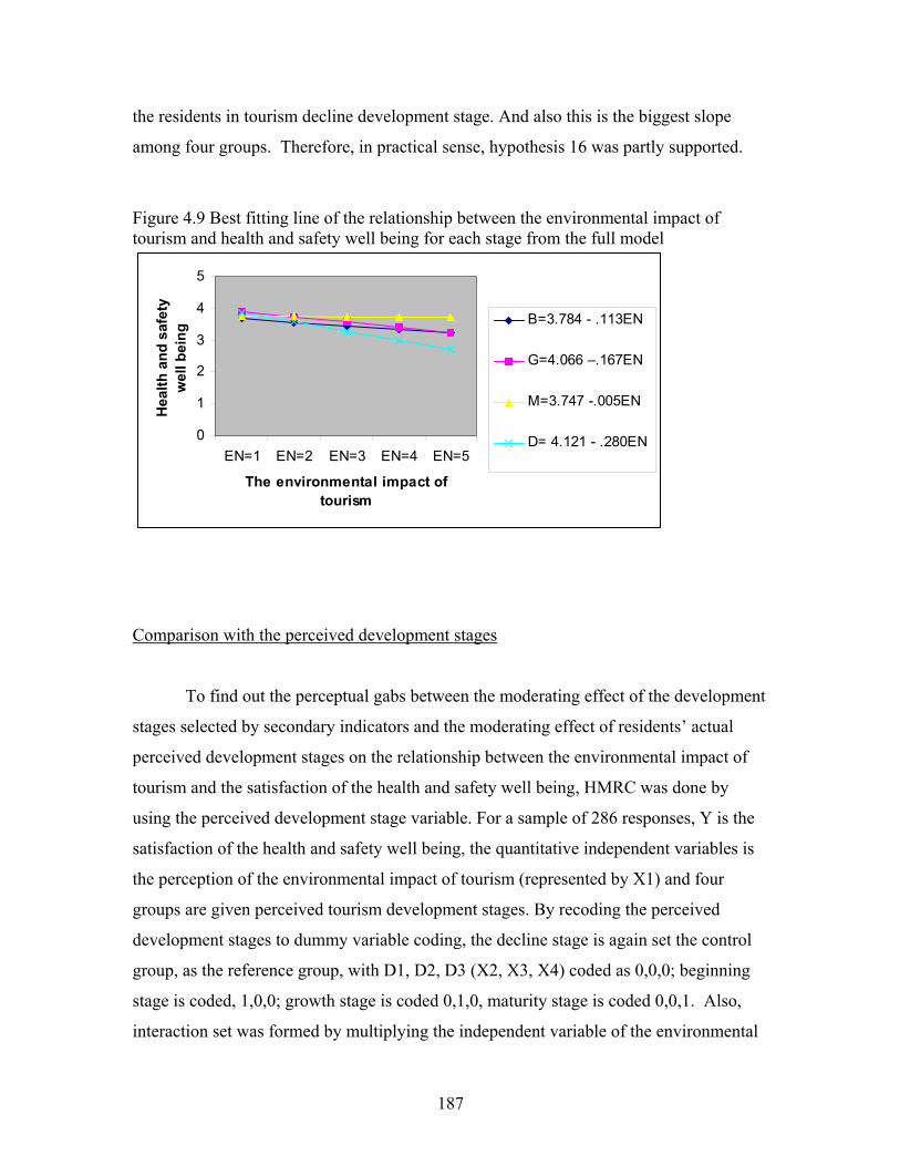
187
the residents in tourism decline development stage. And also this is the biggest slope
among four groups. Therefore, in practical sense, hypothesis 16 was partly supported.
Figure 4.9 Best fitting line of the relationship between the environmental impact of tourism and health and safety well being for each stage from the full model
0
1
2
3
4
5
EN=1 EN=2 EN=3 EN=4 EN=5
The environmental impact of tourism
Hea
lth a
nd s
afet
y w
ell b
eing
B=3.784 - .113EN
G=4.066 –.167EN
M=3.747 -.005EN
D= 4.121 - .280EN
Comparison with the perceived development stages
To find out the perceptual gabs between the moderating effect of the development
stages selected by secondary indicators and the moderating effect of residents’ actual
perceived development stages on the relationship between the environmental impact of
tourism and the satisfaction of the health and safety well being, HMRC was done by
using the perceived development stage variable. For a sample of 286 responses, Y is the
satisfaction of the health and safety well being, the quantitative independent variables is
the perception of the environmental impact of tourism (represented by X1) and four
groups are given perceived tourism development stages. By recoding the perceived
development stages to dummy variable coding, the decline stage is again set the control
group, as the reference group, with D1, D2, D3 (X2, X3, X4) coded as 0,0,0; beginning
stage is coded, 1,0,0; growth stage is coded 0,1,0, maturity stage is coded 0,0,1. Also,
interaction set was formed by multiplying the independent variable of the environmental
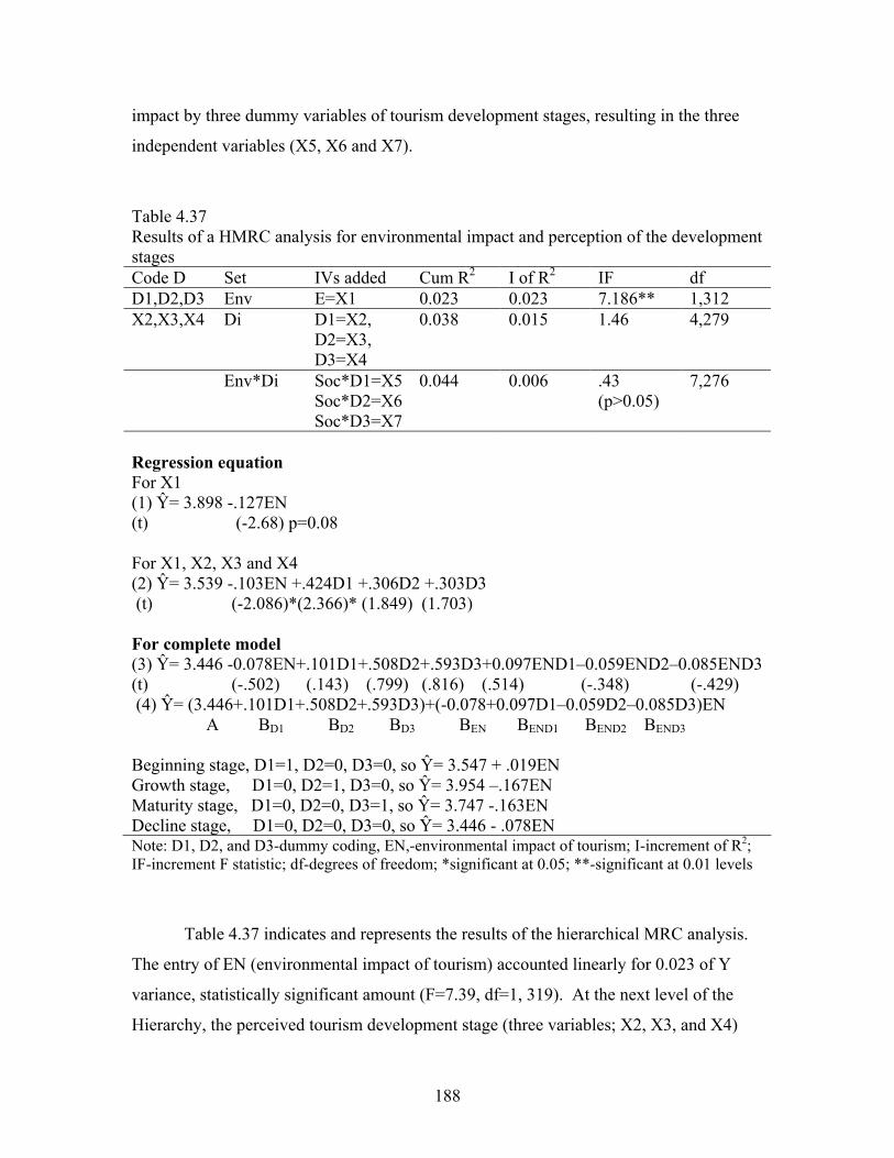
188
impact by three dummy variables of tourism development stages, resulting in the three
independent variables (X5, X6 and X7).
Table 4.37 Results of a HMRC analysis for environmental impact and perception of the development stages Code D Set IVs added Cum R2 I of R2 IF df D1,D2,D3 Env E=X1 0.023 0.023 7.186** 1,312 X2,X3,X4 Di D1=X2,
D2=X3, D3=X4
0.038 0.015 1.46
4,279
Env*Di Soc*D1=X5 Soc*D2=X6 Soc*D3=X7
0.044 0.006 .43 (p>0.05)
7,276
Regression equation For X1 (1) Ŷ= 3.898 -.127EN (t) (-2.68) p=0.08 For X1, X2, X3 and X4 (2) Ŷ= 3.539 -.103EN +.424D1 +.306D2 +.303D3 (t) (-2.086)*(2.366)* (1.849) (1.703) For complete model (3) Ŷ= 3.446 -0.078EN+.101D1+.508D2+.593D3+0.097END1–0.059END2–0.085END3 (t) (-.502) (.143) (.799) (.816) (.514) (-.348) (-.429) (4) Ŷ= (3.446+.101D1+.508D2+.593D3)+(-0.078+0.097D1–0.059D2–0.085D3)EN A BD1 BD2 BD3 BEN BEND1 BEND2 BEND3 Beginning stage, D1=1, D2=0, D3=0, so Ŷ= 3.547 + .019EN Growth stage, D1=0, D2=1, D3=0, so Ŷ= 3.954 –.167EN Maturity stage, D1=0, D2=0, D3=1, so Ŷ= 3.747 -.163EN Decline stage, D1=0, D2=0, D3=0, so Ŷ= 3.446 - .078EN Note: D1, D2, and D3-dummy coding, EN,-environmental impact of tourism; I-increment of R2; IF-increment F statistic; df-degrees of freedom; *significant at 0.05; **-significant at 0.01 levels
Table 4.37 indicates and represents the results of the hierarchical MRC analysis.
The entry of EN (environmental impact of tourism) accounted linearly for 0.023 of Y
variance, statistically significant amount (F=7.39, df=1, 319). At the next level of the
Hierarchy, the perceived tourism development stage (three variables; X2, X3, and X4)
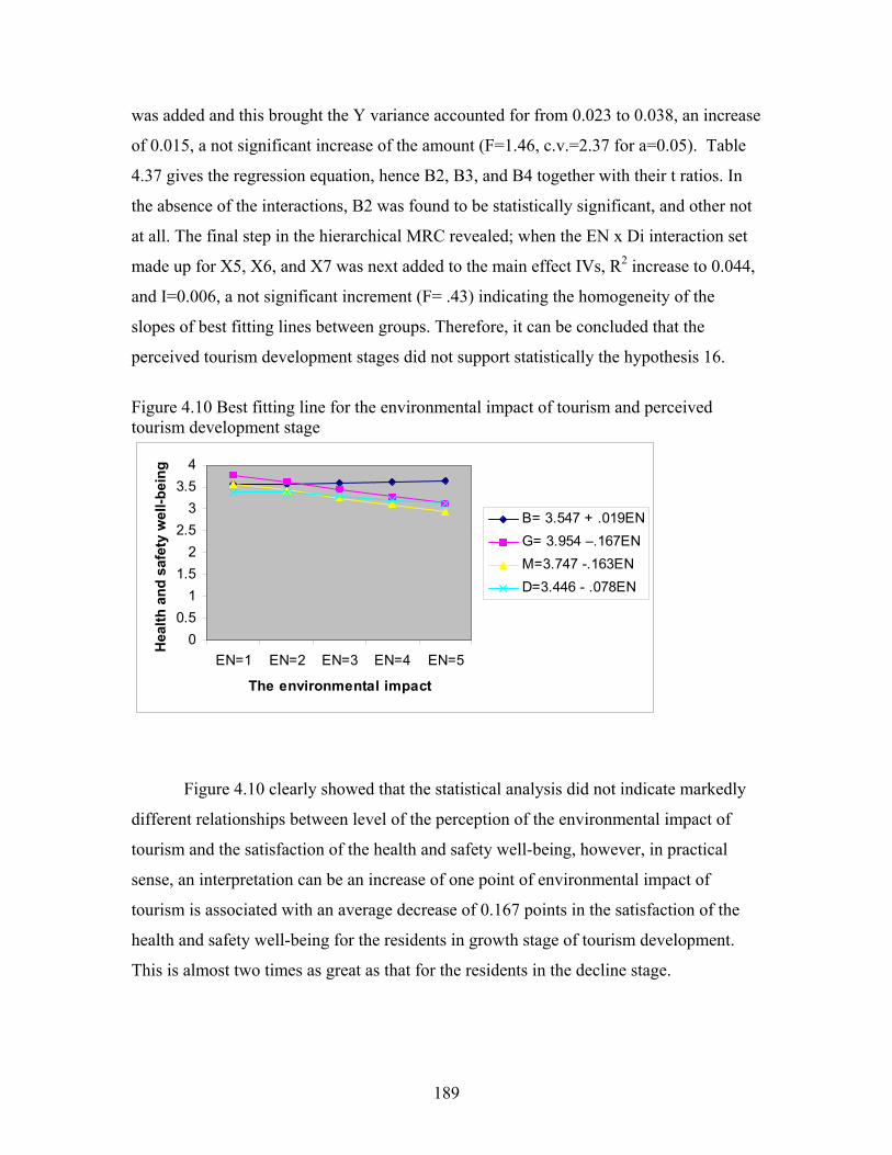
189
was added and this brought the Y variance accounted for from 0.023 to 0.038, an increase
of 0.015, a not significant increase of the amount (F=1.46, c.v.=2.37 for a=0.05). Table
4.37 gives the regression equation, hence B2, B3, and B4 together with their t ratios. In
the absence of the interactions, B2 was found to be statistically significant, and other not
at all. The final step in the hierarchical MRC revealed; when the EN x Di interaction set
made up for X5, X6, and X7 was next added to the main effect IVs, R2 increase to 0.044,
and I=0.006, a not significant increment (F= .43) indicating the homogeneity of the
slopes of best fitting lines between groups. Therefore, it can be concluded that the
perceived tourism development stages did not support statistically the hypothesis 16.
Figure 4.10 Best fitting line for the environmental impact of tourism and perceived tourism development stage
00.5
11.5
22.5
33.5
4
EN=1 EN=2 EN=3 EN=4 EN=5
The environmental impact
Hea
lth a
nd s
afet
y w
ell-b
eing
B= 3.547 + .019ENG= 3.954 –.167ENM=3.747 -.163END=3.446 - .078EN
Figure 4.10 clearly showed that the statistical analysis did not indicate markedly
different relationships between level of the perception of the environmental impact of
tourism and the satisfaction of the health and safety well-being, however, in practical
sense, an interpretation can be an increase of one point of environmental impact of
tourism is associated with an average decrease of 0.167 points in the satisfaction of the
health and safety well-being for the residents in growth stage of tourism development.
This is almost two times as great as that for the residents in the decline stage.
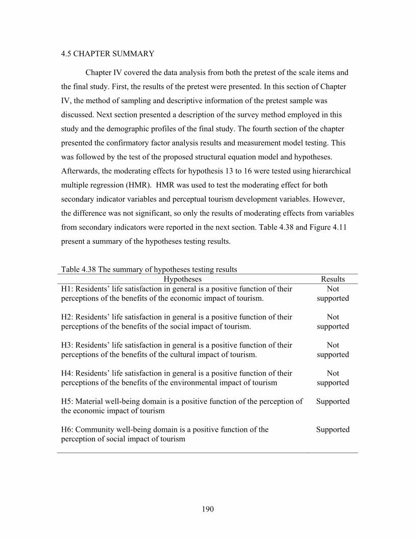
190
4.5 CHAPTER SUMMARY Chapter IV covered the data analysis from both the pretest of the scale items and
the final study. First, the results of the pretest were presented. In this section of Chapter
IV, the method of sampling and descriptive information of the pretest sample was
discussed. Next section presented a description of the survey method employed in this
study and the demographic profiles of the final study. The fourth section of the chapter
presented the confirmatory factor analysis results and measurement model testing. This
was followed by the test of the proposed structural equation model and hypotheses.
Afterwards, the moderating effects for hypothesis 13 to 16 were tested using hierarchical
multiple regression (HMR). HMR was used to test the moderating effect for both
secondary indicator variables and perceptual tourism development variables. However,
the difference was not significant, so only the results of moderating effects from variables
from secondary indicators were reported in the next section. Table 4.38 and Figure 4.11
present a summary of the hypotheses testing results.
Table 4.38 The summary of hypotheses testing results Hypotheses Results
H1: Residents’ life satisfaction in general is a positive function of their perceptions of the benefits of the economic impact of tourism.
Not supported
H2: Residents’ life satisfaction in general is a positive function of their perceptions of the benefits of the social impact of tourism.
Not supported
H3: Residents’ life satisfaction in general is a positive function of their perceptions of the benefits of the cultural impact of tourism.
Not supported
H4: Residents’ life satisfaction in general is a positive function of their perceptions of the benefits of the environmental impact of tourism
Not supported
H5: Material well-being domain is a positive function of the perception of the economic impact of tourism
Supported
H6: Community well-being domain is a positive function of the perception of social impact of tourism
Supported
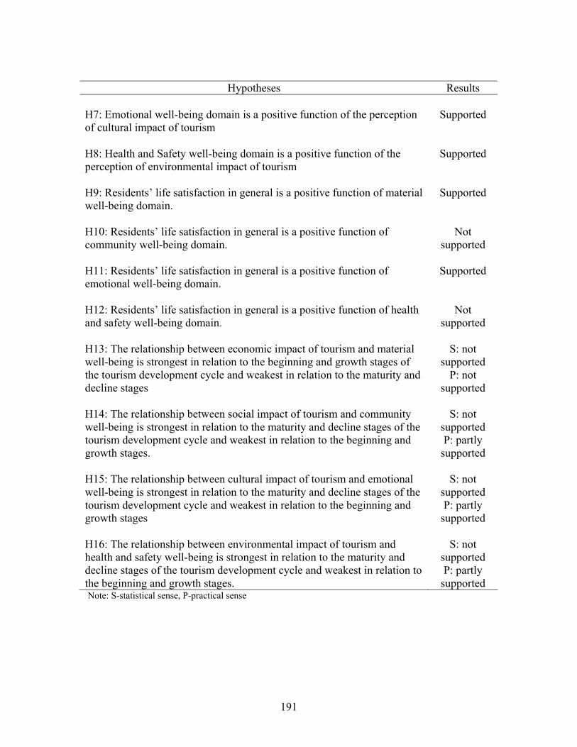
191
Hypotheses Results
H7: Emotional well-being domain is a positive function of the perception of cultural impact of tourism
Supported
H8: Health and Safety well-being domain is a positive function of the perception of environmental impact of tourism
Supported
H9: Residents’ life satisfaction in general is a positive function of material well-being domain.
Supported
H10: Residents’ life satisfaction in general is a positive function of community well-being domain.
Not supported
H11: Residents’ life satisfaction in general is a positive function of emotional well-being domain.
Supported
H12: Residents’ life satisfaction in general is a positive function of health and safety well-being domain.
Not supported
H13: The relationship between economic impact of tourism and material well-being is strongest in relation to the beginning and growth stages of the tourism development cycle and weakest in relation to the maturity and decline stages
S: not supported
P: not supported
H14: The relationship between social impact of tourism and community well-being is strongest in relation to the maturity and decline stages of the tourism development cycle and weakest in relation to the beginning and growth stages.
S: not supported P: partly
supported
H15: The relationship between cultural impact of tourism and emotional well-being is strongest in relation to the maturity and decline stages of the tourism development cycle and weakest in relation to the beginning and growth stages
S: not supported P: partly
supported
H16: The relationship between environmental impact of tourism and health and safety well-being is strongest in relation to the maturity and decline stages of the tourism development cycle and weakest in relation to the beginning and growth stages.
S: not supported P: partly
supported Note: S-statistical sense, P-practical sense

192
The next chapter will discuss the implications of the findings of this study in
greater detail, as well as discuss the limitation of this study and what direction research
should take along the line of the focus of this study.

193
Figure 4.11. The results of the empirical model and the hypotheses tests
** significant at a=0.01 levels, bold numbers show the most strongest relationship among tourism development stages.
Emotional well-being domain
Economic Material well-being domain
Social
Cultural
Environmental
Community well-being domain
Tourism development cycle: Beginning, Growth, Maturity, Decline
Health & Safety well-being
0.37**
0.40**
0.17**
0.24**
0.36**
-0.08
0.58**
0.12
-0.12
0.01
0.10
0.11
QOL
.277, .133, .425, .157
.231, -.023, .127, .245
-.113, -.167, -.005, -.280
.317, .150, .473, .23
CHAPTER V
DISCUSSION AND CONCLUSION
5.1 INTRODUCTION
This chapter presents the summary, discussion and implications of the findings of
the study. In the first section of the chapter, a summary and discussion of the hypotheses
testing are presented. The managerial and theoretical implications of the findings,
followed by the limitation of the study, are discussed next. Finally, the chapter concludes
with suggestions for future research.
5.2 SUMMARY OF THE FINDINGS
This study developed a “tourism impact on quality of life model” that investigates
how tourism impact affects the quality of life of residents in tourism destinations. The
proposed theoretical model addresses satisfaction with life in general, derived from
satisfaction with a particular life domain. For example, overall life satisfaction is derived
from the material well-being domain, which includes the consumer’s sense of well-being
as it is related to material possessions. The satisfaction of this particular life domain in
formulating general life satisfaction is affected by various tourism impact dimensions,
among them economic, social, cultural, and environmental impacts of tourism. Finally,
the tourism development stage moderates the relationships between tourism impact
dimensions and particular life domains. The proposed model in Figure 3.1 was
empirically tested. This model analyzed (1) the effect of residents’ perception of the
economic, social, cultural, and environmental impact of tourism on overall life
satisfaction; (2) the effects of residents’ perception of four tourism impact dimensions on
the satisfaction of particular life domains (material, community, emotional, and health
194
and safety well being); (3) the effect of the satisfaction of four particular life domains on
overall life satisfaction; and (4) the effect of tourism development stages on the
relationship between the perception of tourism impact and the satisfaction of particular
life domains. Before conducting the actual study, a pretest was done to make sure that the
proposed constructs and the items that are proposed to measure those constructs are valid
and reliable.
The study specially focused on a population consisting of residents residing in
Virginia. The sample for this study was proportionally stratified on the basis of the
number of populations in the pre-selected regions in relation to tourism development
stages that covered counties and cities in the state. The study addressed the effects of
tourism on the quality of life of residents in the community. Respondents were asked to
complete a survey based on their perception of tourism impact and their satisfaction of
various life conditions. The result was a final usable sample size of 321 residents in the
community. More than half of the respondents were male; the average age of the
respondents was 53 years old. The demographic characteristics of respondents were
consistent with the previous studies that survey in the similar areas. For example,
Jurowski (1994) reported that the average age of the respondents was 48; Neal (2000)
reported that the average age for the respondents was 56.6; and Gursoy (2001) reported
that the average age of the respondents was 49.
This study developed and tested a measurement model for the sub-dimensions of
each construct through a pretest and an actual test. Results confirmed that each construct
consisted of more than 2 sub-dimensions. Each sub-dimension of the constructs was
measured by at least three indicators. A score of items for each sub-dimension was
summated and used to measure proposed constructs.
The results of the study found that the perception of tourism impact influenced the
satisfaction of particular life domains, and that satisfaction of particular life domains did
affect residents’ overall life satisfaction. However, the perception of tourism impact did
not directly influence overall life satisfaction. In addition, the moderating effects on the
relationships between tourism impact dimensions and particular life domains were not
statistically significant. These findings are discussed in detail in the following section.
195
5.3 DISCUSSION OF THE FINDINGS
The discussion section first addresses the development and testing of tourism
impact dimensions and particular life domains. Four tourism dimensions, four particular
life domains, and overall quality of life variables were discussed in detail in Chapter II in
order to provide a better understanding of the impact of tourism on quality of life. The
dimensions of tourism impact are economic, social, cultural, and environmental;
particular life domains are material well-being, community well-being, emotional well-
being, and health and safety well-being. Each construct consisted of two or three sub-
dimensions. In Chapter III, a multiple indicator measurement scale was developed for
each sub-dimension of constructs.
In Chapter IV, a pretest was first conducted on measurement scales for each sub-
dimension. Examination of the Cronbach Alpha reliability estimate of each sub-
dimension indicated that most sub-dimensions of tourism impact and particular life
domain constructs have a Cronbach Alpha reliability estimate higher than 0.70 except for
three dimensions, which are social problem (.69) in social impact of tourism, spiritual
well-being (.66) in the emotional well-being domain, and health well-being (.60) in the
health and safety well being domain. Since reliability estimates that are between .60 and
.70 represent the lower limit of acceptability (Hair et al., 1998), those three dimensions
were included in the final study.
Next a confirmatory factor analysis was conducted on the data collected from 321
respondents who reside in Virginia. Confirmatory factor analysis resulted in elimination
of some indicators from the proposed model to preserve the unidimensionality of each
scale. Items that remained after this step were presented in Appendix G. Assessing each
sub-dimension of the economic and social impact of tourism construct individually
resulted in no change of the indicators in sub-dimensions. Results indicated that all four
sub-dimensions for the economic impact of tourism and two sub-dimensions for the
social impact of tourism had measurement unidimensionality greater than 0.80 of the
composite reliability estimate. However, the cultural impact of tourism, unlike that
shown in the pretest, had an occurrence of a loading greater than 1.0 for deterioration of
the local service sub-dimension. Therefore, it was deleted before goodness-of-fit was
196
assessed. After this procedure was repeated several times, the four observed indicators
were selected to measure the cultural impact of tourism. The result of the composite
reliability was .88. Assessing each sub-dimension of the environmental impact of tourism
construct individually, and deleting indicators that had large residuals or wanted to load
on other constructs, resulted in decreases in the number of indicators in three sub-
dimensions.
Assessing two sub-dimensions of the material well-being domain individually
resulted in no change in the number of indicators. Five observed variables proposed to
assess the community well-being construct were decreased to four indicators from five.
Two sub-dimensions for material well-being and community well-being had reliability
scores of .87, 84,and 82, respectively. However, the confirmatory factor analysis of
emotional well-being resulted in emotional well-being measured by four observed
indicators with a composite reliability of .67. In addition, assessing each sub-dimension
of health and safety, and deleting indicators that had large error variance or/and large
residuals and wanted to load on other constructs, resulted in a decrease in the number of
indicators in the sub-dimensions. Two decreased sub-dimensions from three of the health
and safety well-being construct had greater than .70 and exceeded the requirement for an
acceptable level.
Finally the overall measurement model for nine constructs was done to check the
unidimensionality of the scales to measure each construct. The results showed that the
summated indicators used to measure the economic impact of tourism decreased to three
summated indicators from four after elimination of “cost of living,” which did not work
out (a loading value was 0.1). The summated indicator “social problem” used to measure
the social impact of tourism construct also did not work out when measuring the social
impact of tourism. After eliminating the social problem variable, the social impact of
tourism was measured by three observed variables represented by a local service sub-
dimension. The final indicators for nine constructs were three summated indicators for
the economic impact of tourism, three observed indicators for the social impact of
tourism, four observed indicators for the cultural impact of tourism, three observed
indicators for the environmental impact of tourism, two summated indicators for material
well-being, two observed indicators for community well-being, three observed indicators
197
for emotional well-being, two summated indicators for health and safety well-being, and
three observed indicators for the overall quality of life measure.
Findings of this study are consistent with assumptions that the economic impact
of tourism dimension may have sub-dimensions. However, other tourism impact
dimensions did not reveal various sub-dimensions. Many previous researchers have
reported that each tourism impact dimension has both positive and negative impacts
(Andereck, 1995; Ap & Crompton, 1998; Crandall, 1994; Farrell & Runyan, 1991; Gunn,
1988; Mathieson & Wall, 1984; Murphy, 1985; Tosun, 2002; Weaver & Lawton, 2001;
Witt, 1990). The results of this study indicated that when residents in the community
were asked to reveal tourism impacts, they assessed the perception of tourism impact in
both negative and positive ways (from the unidimensionality check for each individual
sub-dimension, all sub-dimensions for each tourism impact were significant), but when
their tourism impacts were perceived in relation to their life satisfaction, their positive
perceptions were strong with regard to the economic, social, and cultural impact of
tourism, but negative perceptions were strong regarding the environmental impact of
tourism. For example, a previous study about cultural impact of tourism suggested that
residents’ perceptions of tourism destinations showed a negative effect on the evolution
of cultural traditions (Belisle & Hoy, 1980; Liu et al., 1987), but Virgin Islanders
exhibited consensus that tourists seem to respect local traditions and cultures and want to
know more about the residents. However, the results of this study revealed that the
overall measurement for the cultural impact of tourism was statistically significant only
when it consisted of positive perception indicators, such as meeting tourists from all over
the world or cultural exchange between residents and tourists, which was deemed
valuable for the residents.
The findings about quality of life studies are a little bit different from the previous
studies. The particular life domains have usually measured only one or several observed
indicators without sub-dimensions. For example, Gerlach and Stephen (1997) concluded
that unemployment plays a significant role in subjective well-being in their study of
unemployment and subjective well-being between East and West Germans. Like these,
work plays an important role in subjective well-being. Lane (1991) also argues that
subjective well-being is affected by financial well-being. This is because those who feel
198
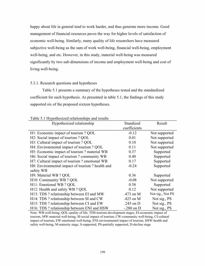
happy about life in general tend to work harder, and thus generate more income. Good
management of financial resources paves the way for higher levels of satisfaction of
economic well-being. Similarly, many quality of life researchers have measured
subjective well-being as the sum of work well-being, financial well-being, employment
well-being, and etc. However, in this study, material well-being was measured
significantly by two sub-dimensions of income and employment well-being and cost of
living well-being.
5.3.1. Research questions and hypotheses
Table 5.1 presents a summary of the hypotheses tested and the standardized
coefficient for each hypothesis. As presented in table 5.1, the findings of this study
supported six of the proposed sixteen hypotheses.
Table 5.1 Hypothesized relationships and results Hypothesized relationship Standized
coefficients Result
H1: Economic impact of tourism ? QOL -0.12 Not supported H2: Social impact of tourism ? QOL 0.01 Not supported H3: Cultural impact of tourism ? QOL 0.10 Not supported H4: Environmental impact of tourism ? QOL 0.11 Not supported H5: Economic impact of tourism ? material WB 0.37 Supported H6: Social impact of tourism ? community WB 0.40 Supported H7: Cultural impact of tourism ? emotional WB 0.17 Supported H8: Environmental impact of tourism ? health and safety WB
-0.24 Supported
H9: Material WB ? QOL 0.36 Supported H10: Community WB ? QOL -0.08 Not supported H11: Emotional WB ? QOL 0.58 Supported H12: Health and safety WB ? QOL 0.12 Not supported H13: TDS ? relationship between EI and MW .473 on M Not sig., Not PS H14: TDS ? relationship between SI and CW .425 on M Not sig., PS H15: TDS ? relationship between CI and EW .245 on D Not sig., PS H16: TDS ? relationship between ENI and HSW -.280 on D Not sig., PS Note: WB-well-being, QOL-quality of life, TDS-tourism development stages, EI-economic impact of tourism, MW-material well-being, SI-social impact of tourism, CW-community well-being, CI-cultural impact of tourism, EW-emotional well-being, ENI-environmental impact of tourism, HSW-health and safety well-being, M-maturity stage, S-supported, PS-partially supported, D-decline stage
199
Hypothesis 14, 15 and 16 were not statistically significant, but they, in a practical sense,
were partially supported. Seven of the sixteen hypotheses were not supported. Even
though hypotheses 1 through 4 were not supported, the results indicated that the effect of
tourism impacts altogether (four tourism dimensions) significantly explained 3.6% of the
total variance of overall life satisfaction. The rest of the section addresses the research
question and the hypotheses that were empirically tested.
Research question I
Does tourism affect the quality of life of residents in a community?
Research question I was addressed by four hypotheses: H1: Residents’ life
satisfaction in general is a positive function of their perceptions of the benefits of the
economic impact of tourism; H2: Residents’ life satisfaction in general is a positive
function of their perceptions of the benefits of the social impact of tourism; H3:
Residents’ life satisfaction in general is a positive function of their perceptions of the
benefits of the cultural impact of tourism; and H4: Residents’ life satisfaction in general
is a positive function of their perceptions of the benefits of the environmental impact of
tourism. Findings of this study supported the research question (all tourism impacts
significantly explained 3.6% of the total variance of overall life satisfaction) but did not
support individually proposed hypotheses that there are direct, positive relationships
between various dimensions of tourism impact and overall life satisfaction. However, it
should be noted that even though the effect of each tourism impact dimension on overall
life satisfaction did not show statistical significance, some sense of the direct effects of
tourism impact on overall life satisfaction still existed. .
The result reported here is consistent with previous research findings. Even
though there was no study to test the direct effects from various dimensions of tourism
impact on overall life satisfaction of residents in the community, some of the previous
study findings suggest: that residents perceived an improvement in income, standard of
living, investments and business activities ensuing from tourism activities (Liu & Var,
1986); that cultural exchange between residents and tourists was valuable (Liu et al.,
200
1987; Belisle & Hoy, 1980); and that the negative effects of noise, litter, and air and
water quality on the community are perceived (Pizam, 1978; Lankford & Howard,
1994). However, this study showed that residents’ positive perception of each dimension
of tourism impact did not have a statistically significant effect on their overall life
satisfaction. In addition, the result of this study revealed that there was a negative
relationship (even though this was not statistically significant) between the perception of
the economic impact of tourism and overall life satisfaction (-0.12). Even though Perdue
at al’s study (1999) reported that changes in job opportunities had very little influence on
perceived QOL, they did mention that economic benefits are not sufficient but clearly
necessary condition. This result can be explained: in a sense, residents in a community
may feel relative poorness when they perceive the positive economic impact of tourism.
For example, when a resident who has a job unrelated to tourism perceives an improved
economic situation, or an increment of employment opportunity (one positive economic
impact) in the community, he or she may think that the positive economic impact of
tourism affects others’ lives who have tourism-related jobs but not his or her own. This
study revealed that only 19% of the respondents answered that a small portion (an
average of 12%) of their income comes from tourism. In addition, Crotts and Holland
(1993) showed that tourism affects positively the quality of life of rural residents in terms
of income, health, recreation, personal services and per capita sales, and negatively
affects the level of poverty. Therefore, this study concludes that holistically, tourism
impact did affect residents’ life satisfaction in general; however, a specific dimension of
tourism impact did not affect directly their overall life satisfaction.
Research Question 2:
Does tourism impact affect particular life domains?
The second research question addresses the influence of tourism impact on
particular life domains. These relationships were examined through hypothesis 5, 6, 7,
and 8 (H5: Material well-being domain is a positive function of the perception of the
economic impact of tourism; H6: Community well-being domain is a positive function of
201
the perception of social impact of tourism; H7: Emotional well-being domain is a positive
function of the perception of cultural impact of tourism; and H8: Health and Safety well-
being domain is a positive function of the perception of environmental impact of
tourism). All four hypotheses were supported; the examination of these hypotheses
revealed the strength and direction of the relationships between four dimensions of
tourism impact and particular life domains.
Once a community becomes a destination, the lives of residents in the community
are affected by tourism (Jurowski, 1994). The development of tourism affects the lives of
residents in better or worse ways. These life conditions make up the life domains in
general. Usually, the perceptions of tourism impact influence these life conditions.
Therefore, satisfaction or dissatisfaction with living condition (e.g., employment and
income), influenced by the perception of the tourism, spill over vertically to satisfaction
with life domains. Consequently, satisfaction of a particular life condition influences the
overall life satisfaction of residents.
Like other studies, this study found a positive relationship between the economic
impact of tourism and material well-being related to consumers’ sense of well being as it
is related to material possessions. As previous studies have reported, tourism increases
the standard of living of host residents, helps generate employment, and increases
revenues to local business (Backman & Backman, 1997; Krohn, 1992, 1995; Var & Kim,
1990). This study found that the residents’ perception of these economic impacts of
tourism positively affected their satisfaction of material well-being. This study also
confirms that Cummins’ (1996) study that the satisfaction of material well-being domain
mostly comes from the economic situation, income, living situation, standard of living,
housing, financial situation, and personal possessions, is valid.
This study finding was also consistent with previous studies in terms of the
positive relationship between the social impact of tourism and community well-being
(H6), meaning that as residents increasingly perceive the positive social impact of
tourism, their satisfaction of the community well-being increase. In the study of Backman
and Backman (1997), and Var and Kim (1990), residents in the community agreed that
shopping facilities built to serve tourists also serve residents, that services of all kinds
established and offered to tourists in turn serve local residents, and that tourism generates
202

the impetus to improve and further develop community infrastructure. Perdue, Long and
Kang (1999) studied how residents’ perception of community safety, community
involvement, local political influence, and changes in job opportunities, social
environment, and community congestion influenced their quality of life in the
community. Their findings showed that the key community characteristics affecting
residents’ QOL were community safety, social environment, and community
involvement. Cummins (1997) found that the satisfaction associated with the community
well-being domain occurs when people achieve satisfaction with education,
neighborhood, service and facilities, social life, and social relation. As the results of
previous studies, this study finds that residents’ perception of the positive social impact
of tourism affects their satisfaction and sense of community well-being in the form of
services and facilities related to residents’ community life.
In addition, this study found that the relationship between the cultural impact of
tourism and emotional well-being is significantly positive (H7), meaning that the positive
perception of the cultural impact of tourism, such as “I would like to meet tourists from
as many countries as possible in order to learn about their culture” and “the cultural
exchange between residents and tourists is valuable for the residents,” increases
residents’ satisfaction of emotional well-being related to spare time, leisure life, and
cultural life. This result is also consistent with the findings of previous studies. Var and
Kim (1990) reported that tourism contributes to the renaissance of traditional arts and
crafts, and helps promote understanding of different people through cultural exchange.
Tourism also helps keep culture alive; helps preserve traditional art forms; maintains
cultural identity and passing on the cultural beliefs and rituals to the next generation
(Chen 1997; Var & Kim, 1990). Staats et al. (1992) examined family patterns in the use
of free time. The study reveals that most people spend most of their leisure time with
family and friends and that they desire to do so. Argyle and Lu (1990) found that leisure
activities fall into at least two major categories such as teams and clubs, dances, parties,
debates, and meeting new people. Residents’ positive awareness of the cultural exchange
between tourists and residents influences the emotional satisfaction of meeting new
people and having a good time.
203
Lastly, this study found that there is a positive relationship between the
environmental impact of tourism and health and safety well-being (H8). Researchers
have found that tourism helps create greater awareness and appreciation for the need to
preserve the environment to preserve its natural beauty for tourist purposes (Var & Kim
1990). As Bubloz et al. (1980) noted the environment is the place that provides
sustenance of the human environed unit. Thus, the environment should be preserved and
enhanced to provide sufficient resources to meet those needs of the human units within it.
If a resident perceives the positive environmental impact of tourism, he/she will have
satisfaction regarding the environment; this effect will give him/her a sense of health,
safety, and well-being. However, often tourism has been considered as a negative
influence on the environment, in the form of the destruction of natural resources, the
deterioration of cultural and historical sites, or the production of litter, garbage, and
waste (Var & Kim, 1990). If a resident residing near a seaside lake saw contaminated
water or garbage on the water because of restaurants in that area, he/she might refuse to
drink unpurified water from the tap. If he/she drinks the water from the tap, he/she may
think that he/she will become sick.
In conclusion, this study clearly supported the second research question and its
associated hypotheses. Residents perceived the positive economic, social, and cultural
impact of tourism, and their satisfaction of the related life domain was increased.
However, residents in the community perceived the negative environmental impact of
tourism, and the satisfaction of its associated life domain was decreased statistically
significant.
Research Question 3:
Do the particular life domains affected by tourism impacts affect overall QOL of
the residents in the community?
The third research question addresses the influence of particular life domains on
the overall life satisfaction. The relationship between material well-being and overall life
satisfaction was examined by hypothesis 9. It was hypothesized that there is a positive
relationship between material well-being and residents’ life satisfaction in general. This
204
study indicated that residents’ satisfaction with their material well-being was affected by
the economic impact of tourism (e.g., increasing opportunity for employment).
However, the relationship between community well-being and the overall life
satisfaction examined by hypothesis 10 was not significant, and this result was not
consistent with the previous studies. Cummins (1997) found that the satisfaction
associated with the community well-being domain occurs when people achieve
satisfaction with education, neighborhood, service and facilities, social life and social
relations. Norman et al. (1997) conducted a study showing that community satisfaction
does make a significant and positive contribution to community residents’ perceptions of
their quality of life. The study involved five rural South Carolina communities; it
revealed that satisfaction with recreational services provided by the town does positively
affect community satisfaction. On the other hand, Argyle and Lu (1990) and Andrew and
Withey (1976) measured QOL using the formative concept, made up of happiness and
life satisfaction. The results revealed that fun and family contribute more to happiness
than to life satisfaction. Money, economic security, one’s house, and the goods and
services bought in the market contribute to life satisfaction more than to happiness. Life
satisfaction refers to the satisfaction people may feel toward their overall living
conditions and life accomplishments. Therefore, the community well-being affected by
the social impact of tourism, such as the variety of entertainment in the community, well-
maintained roads and other local services, and more recreational opportunities for local
residents, may contribute to residents’ happiness more than their life satisfaction from
their accomplishments. That can be an explanation that the satisfaction with community
well-being did not affect statistically significant on residents’ overall life satisfaction
The relationship between emotional well-being and life satisfaction was examined
by hypothesis 11. It was hypothesized that there is a positive relationship between overall
life satisfaction and the satisfaction of emotional well-being. This hypothesized positive
relationship was supported by the findings of this study. Findings of this study indicated
that residents’ satisfaction of emotional well-being affected by cultural tourism impacts
significantly influences their overall life satisfaction. The results of this study are
consistent with those of previous studies. Cummins (1997) found that the satisfaction of
emotional well-being domain mostly came from leisure activities, religion, recreation,
205
and hobbies. QOL researchers have conceptualized leisure well-being in terms of: leisure
satisfaction (Neal, Uysal, & Sirgy 1995, 1999: Norman, Harwell, & Allen 1997); leisure-
life experience-construed and measured in terms of leisure boredom (Haggard, Granzin,
& Painter, 1995); satisfaction with non-working activities (Campbell et al., 1976),
amount of fun one is having (Andrews & Withey 1976); spare time activities (Andrew &
Withey 1976); and leisure experience in terms of peace, achievement, exercise, and risk
(Unger & Kernan 1990). Orman, Harwell, and Allen (1997) have conducted a study
showing that leisure satisfaction in one’s community does make a significant and positive
contribution to community residents’ perceptions of their own quality of life. Therefore,
the residents’ satisfaction with leisure life and a cultural life involved with of meeting
tourist or cultural exchange between tourists and residents strongly affected their overall
life satisfaction.
The relationship between health and safety well-being and overall life satisfaction
was examined by hypothesis 12. Hypothesis 12 posits that there is a positive relationship
between overall life satisfaction and the satisfaction of health and safety well-being.
Hypothesis 12 was not supported by the study result. The finding of the study showed
some relationship between the satisfaction of health and safety well-being and overall life
satisfaction, but not enough to be statistically significant. The result of this study was not
consistent with previous findings. Previous research has shown that feelings about
personal health spill over to overall life satisfaction, because personal health is
considered important in one’s evaluation of life (Andrew & Withey 1976). However, the
results of this study did not show the statistical significance of the relationship between
health and safety well-being and overall life satisfaction. Health and safety well-being
itself is truly important in the overall QOL of the residents. However, the components of
health and safety well-being come from many different areas such as the health care
system, environment impacts, the threat of the social crime, and etc. Residents might feel
that threats to health and safety affected by the environmental impact of tourism might
not significantly affect their lives. They may perceive threats from environmental
degradation and waste problems, but they may feel that these are not personal problems
but social problems. On the other hand, residents’ satisfaction with health and safety
well-being may mostly come from the health care system or social security system. In
206
addition, the satisfaction with health and safety well-being influenced by a well-
preserved natural environment spills over into emotional well-being and satisfaction with
leisure activities, not into satisfaction with health and safety well-being.
Research Question 4:
Do residents perceive tourism impacts differently according to tourism
development stages, and do development stages have a moderating effect on the
relationship between tourism impacts and particular life domains?
Research question four addressed the moderating influence of tourism
development stages on the relationship between the dimensions of tourism impact and
particular life domains. These relationships were examined through hypotheses 13, 14,
15, and 16. This research question posits that residents in the community usually start to
perceive the economic impact of tourism in the beginning stage of tourism development,
and feel the benefit of the economic impact of tourism the most at the growth stage of
tourism development. Afterwards, when tourism resources reach their maximum status,
residents in the community start to perceive the impact of social, cultural and
environmental impact of tourism on the maturity stage of tourism development, and feel
their impact strongest at the decline stage of tourism development. However, the results
of this study did not statistically support hypotheses 13 to 16. Even though the study
findings did not indicate the statistical significance of the moderating effects of the
tourism development stage on the relationship between tourism impact dimensions and
particular life domains, the results of this study, in a practical sense, showed that there
were some meaningful moderating effects on the relationships between the dimensions of
tourism impact and particular life domains. The moderating effects of tourism
development on the relationship between the economic impact of tourism and the
satisfaction of material well-being was strongest in the maturity stage; the moderating
effects of tourism development on the relationship between the social impact of tourism
and the satisfaction of community well-being was strongest in the maturity stage. The
207
moderating effects of tourism development on the relationship between the cultural
impact of tourism and the satisfaction of emotional well-being was strongest in the
decline stage; the moderating effects of tourism development on the relationship between
the environmental impact of tourism and the satisfaction of health and safety well-being
was strongest in the decline stage of tourism development. Therefore, hypotheses 13 to
16 were partially supported.
In addition, the results of this study indicated another important finding: that in
the absence of interactions, the economic impact of tourism, adjusted by the mean of the
satisfaction of the material well-being of the growth stage, was significantly higher than
the un-weighted mean of other stages. The social impact of tourism adjusted by the mean
of the satisfaction of the community well-being of the maturity stage was significantly
higher than the un-weighted mean of other stages. The environmental impact of tourism
adjusted by the mean of the satisfaction of the health and safety well-being of the growth
and the maturity stage was significantly higher than the un-weighted mean of other
stages.
Even though the findings of this study did not show statistical significance, the
results of this study were similar to previous findings. In 1988, Allen et al. examined
changes in residents’ perceptions of seven dimensions of community life across 20
communities classified on the basis of the percentage of retail sales derived from tourism.
Their study (1988, p.20) stated that, “Lower to moderate levels of tourism development
were quite beneficial to the study communities, but as development continued, residents’
perceptions of community life declined, particularly as related to public services and
opportunities for citizens’ social and political involvement”, meaning that overall,
residents in the community perceive the benefits of the economic impact of tourism and
the satisfaction of material well-being in the lower to moderate levels of tourism
development, but they are less likely to perceive the benefits of others impact of tourism
(e.g., social, cultural and environmental) and satisfaction with its correspondent life
domains (e.g., community well-being, emotional well-being, and health and safety well-
being, respectively) in those levels of tourism development. On the other hand, residents
in the community perceive the benefits of the social, cultural, and environmental impact
of tourism and the satisfaction with its associated life domains in highest level of tourism
208
development, but they are less likely to perceive the benefits of the economic impact of
tourism and satisfaction with material well-being in that level of tourism development.
Unlike the expectation that the results appear to be a social carrying capacity, this
study results can be found residents’ QOL in England and Albrecht’s (1984) “social
disruption theory”, which postulates that boomtown community initially enter into a
period of generalized crisis, resulting from the traditional stress of sudden, dramatic
increases in demand for public services and improving community infrastructure.
Additionally, resident develop adaptive behaviors that reduce their individual exposure to
stressful situations. Through this process, residents’ QOL is expected to initially decline,
and then improve as the community and its resident adapt to the new situation (Krannich,
Berry & Greider, 1989). This study results showed that the relationship between the
economic impact of tourism and the satisfaction with material well-being initially
decreased in the growth stage of tourism development and peaked in maturity stage of
tourism development. However, when a community enters decline stage of tourism
development, the relationship between the economic impact of tourism and the
satisfaction with material well-being decreased, and the relationship may be considered
to be the capacity of the destination area to absorb tourists before the host population
would feel negative impacts. This is the consistent with the theoretical foundation of
carrying capacity. When tourism reaches its maturity or maximum limit, residents’ QOL
may start deteriorating.
However, the relationship between the cultural impact of tourism and the
satisfaction with emotional well-being decreased in the growth stage of tourism
development, increased in the maturity stage of tourism development, and peaked in the
decline stage of tourism development. Neither the theory of social carrying capacity nor
social disruption offered much to explain this result. However, this result is consistent
with Butler’s (1980) argument that in the decline stage, more tourist facilities disappear
as the area becomes less attractive to tourists and the viability of existing tourist facilities
becomes more available to residents in the destination community.
The relationship between the environmental impact of tourism and the satisfaction
with health and safety well-being increased in the growth stage of tourism development,
decreased in the maturity stage of tourism development, and peaked in the decline stage
209
of tourism development. This result confirms Butler’s (1980) concept of the tourist area
cycle of evolution. As residents’ perception of negative environmental impacts increases,
their satisfaction with health and safety well being decreases in the decline stage of
tourism development unless the area as a destination provides rejuvenating or alternative
planning options.
5.3.2. Summary of the discussion
Overall, the findings of this study indicate that there is a positive relationship
between the impact of tourism and a particular life domain, meaning that as residents’
perception of the positive economic impact of tourism increases, their satisfaction of
material well-being increases too; and that residents’ increased satisfaction of the
material well-being affected by the positive economic impact of tourism finally
influences their overall life satisfaction. Findings also suggest that even though the study
result did not indicate the statistical significance of the moderating effects of the tourism
development stage, it did show that there were some meaningful moderating effects on
the relationship between the dimensions of tourism impact and particular life domains.
5.4. IMPLICATION OF THIS STUDY
5.4.1. Managerial implications
As illustrated by Mathieson and Wall (1982), the nature of planning tourism
destinations is complex. Tourism planners and developers often confront paradoxical
effects when assessing alternative policies. Questions arise concerning how to maximize
benefits and at the same time minimize the cost for residents in the tourism community.
This research provides tourism planners with useful information concerning specific
elements associated with residents’ positive perception of the impact of tourism, their life
satisfaction, and tourism development stages.
Findings of this study are of importance to tourism developers in the tourism
community. Tourism in the community should be developed not simply on the analysis of
210
costs and benefits in the short-term, but also from a long-term perspective of residents’
QOL and sustainable tourism. The findings of this study showed that as residents’
perception of the impact of tourism increases, their life satisfaction with various life
conditions increases, and that this effect finally influences to their overall life
satisfaction. For example, as residents’ perception of the economic impact of tourism
increases, they are more likely to be satisfied with their lives based on material
possessions. In addition, as residents’ perception of the cultural impact of tourism
increases, they are more likely to be satisfied with their lives based on emotional well-
being such as satisfaction of leisure life and spiritual life. Then, the satisfaction with
these specific life domains affects the overall QOL of residents in the community.
Tourism development strategists need to consider the strength of this relationship, and
focus on maintaining the residents’ overall life satisfaction derived from tourism impacts.
This finding also suggests that tourism developers and marketers should know
how residents perceive tourism and how it affects their life satisfaction according to
tourism development stages. If the residents in a community always perceive the impact
of tourism in negative ways, these residents may communicate their negative feelings to
tourists or other residents, and tourism developers’ efforts to get residents’ support may
be useless. The results of this study revealed that the relationship between the economic
impact of tourism and material well-being was strongest in the maturity stage, meaning
that residents strongly perceive the positive economic impact of tourism, and they are
more satisfied with the material well-being domain in a maturity stage. However, as
Butler (1980) mentioned, the maturity stage is called a stagnation stage that the peak
numbers of visitors have been reached, and the capacity level for many variables may
have been reached or exceeded with attendant environmental, social, and economic
problems. Therefore, even though residents perceive a positive impact of tourism
associated with their life satisfaction in the maturity stage that might not last long. Such a
feeling may turn quickly into negative perceptions. So, tourism developers should plan a
strategy that has residents start to perceive positive impact of tourism in the beginning
stage of the development in order to fully recognize the economic impact of tourism in
the growth stage.
211
Findings of this study also showed that relationships between the cultural impact
of tourism and emotional well-being and between the environmental impact of tourism
and health and safety well-being were strongest in the decline stage of tourism
development, meaning that residents perceive a strong positive cultural impact of tourism
in the decline stage, and feel more satisfaction in emotional well-being. This result is
consistent with Burtler (1980)’s study that in the decline stage, more tourist facilities
disappear as the area becomes less attractive to tourists and the viability of other tourist
facilities becomes more questionable. Ultimately, the area may become a veritable tourist
slum or lose its tourist function completely. However, local involvement in tourism is
likely to increase at this stage, as employees and other residents are able to purchase
facilities at significantly lower prices as the market declines. So residents’ perception of
this type of tourism impact is strong in the maturity and decline stages. However,
residents’ positive perceptions may quickly become negative when they perceive the
negative impact of cultural and environmental tourism impacts. In this stage, tourism
developers should try to rejuvenate the tourism destination before that community
completely reaches a maximum carrying capacity and a decline stage.
Individuals seeking to gather support from the community for an already
established tourism industry may find the information provided by this research useful.
The research demonstrates that perception of the positive social impact of tourism was an
important determinant in satisfaction with community well-being. This finding suggests
that internal marketing techniques designed to inform residents of the social benefits they
receive from tourism may be helpful in gaining the residents’ support for the
development, successful operation and sustainability of tourism. Promotion of the
positive social and economic benefits of tourism may serve to sway the opinion of
residents who perceive that they have little to gain economically from the tourism
industry. Further, the dissemination of information concerning secondary economic
benefits received by community members whose household income is not directly tied to
the tourism industry may lead to support from otherwise neutral residents. The
application of conservation and preservation programs for the community may serve to
ease the concerns of residents who are skeptical to the environmental impact of tourism.
212

In addition, the measurement instrument refined and tested in this study should be
used via a mail survey to periodically and spatially appraise how well the residents in the
community perceive tourism impact and how they receive this impact regarding their
satisfaction with what the industry is doing in terms of enhancing the QOL of the
residents in the community. Also the data generated by periodically administering the
survey to residents, tourism developers and managers (CBV directors or persons related
to tourism industry) can be examined and compared with the mean score of the
perceptions of tourism impact and life satisfaction. However, one thing should be noted:
that while the same conclusions may not be appropriate for all rural communities
considering tourism development, the tools developed for this research might be useful in
other communities. Through application of the principles determined by this research, the
strength of each factor in determining support for alternative plans could be ascertained
in a variety of tourism settings.
5.4.2. Theoretical implications
The significant contribution of this study was the discovery of which
determinants of satisfaction with the particular life domains are involved with the
particular dimension of tourism impact, and that overall life satisfaction consists of the
particular life domains. Perhaps most importantly, the findings demonstrated that factors
that influence residents’ QOL are multi-dimensional and dynamic. The study
demonstrated how the economic impact of tourism influences the satisfaction with
material well-being; and that the cultural impact of tourism affects overall life
satisfaction positively through its interaction with perceptions of the social impact of
tourism. The examination of the interplay of several elements provides information about
which tourism impact dimension influences which particular life domain, and an
explanation of why the relationship between the perception of tourism impact and the
satisfaction of the particular life domains vary according to levels of tourism
development within the same community. Furthermore, while conclusive evidence has
demonstrated the strong positive relationship between the perception of tourism impact
and residents’ overall QOL (Perdue et al, 1990), this study revealed how the economic
213
impact of tourism influences the satisfaction of material well-being, and this satisfaction
of the material well-being affects residents’ overall life satisfaction. The discovery of the
direct effect among the four types of tourism impacts on the satisfaction of four different
life domains provides new information concerning the power of each type of impact to
influence residents’ final QOL.
This study contributes to the theoretical advancement in the field of tourism by
confirming the usefulness of carrying capacity theory and the tourism development cycle
principle in explaining host community residents’ satisfaction through tourism. Life
satisfaction, an important element to host community residents, was identified as a
critical factor when the tourism planners try to extract residents’ support for tourism
development. When residents perceive the impact of tourism, then when they satisfy with
tourism, finally they will support for tourism. The findings demonstrated that factors
heretofore thought to influence residents’ life satisfaction also influence their overall life
satisfaction and in doing so have a greater effect on support for tourism.
The model developed and tested in this research provides a theoretical basis for
the study of support for tourism in a variety of settings. The model can be utilized to
compare communities with different social structures or at different stages of tourism
development to determine changes in the interplay among the elements. New elements
can be added to the model, which may further explain residents’ satisfaction of a specific
life domain from tourism. In addition, the proposed tourism impact model contributes a
theoretical foundation for the examination of the relationship between the impact of
tourism, satisfaction from various life conditions, and residents’ overall life satisfaction.
The theoretical model may be helpful in directing future research in determining, first,
the elements being examined by the various components in the model. Once these are
identified and evaluated, research may be focused on the dynamic components and/or the
influence and role of each structure in the model.
214

5.5 LIMITATIONS OF THE STUDY
One limitation of the study was that the sample population of the study consisted
of residents residing in pre-selected cities and counties of Virginia based on four
secondary indicators. The secondary indicators were Population Growth Rate (PGR),
Traveler Spending Growth Rate (TSGR), Direct Travel Employment Growth Rate
(DTEGR), and State Travel Tax Growth Rate (STTGR). This means that the area
selected for tourism development stages did not fully cope with the tourism development
stages from the literature. Haywood (1986) and Butler (1980) divided the areas into
different stages by using tourist arrivals. If the areas had been selected by using the
number of visitors to a community, the results might have been different. However, it
was difficult to count the exact number of visitors for a community. This may be one of
the solutions if you divide the area according to its CVB (convention and visitors’
Bureau) territory, not by its political territory, because CVB counts roughly the number
of visitors.
In addition, this study was focused only on residents in Virginia. It is possible that
if the study was conducted on the other residents of other states and counties, the
magnitude and direction of the relationship between tourism impact and overall life
satisfaction might be different. Also, if the survey was extended to include business
people, tourism planners, or other kinds of stakeholders in the tourism community, there
may be different levels of influence of perception of tourism impact on overall life
satisfaction. Including many residents in other sectors may help us better understand the
relationship between tourism impacts and life satisfaction and the role of tourism
development stages.
This study examined the influence of four-tourism impact dimensions on four
specific well-being domains. One limitation is related to testing only the influences of
one tourism impact dimension on one particular life domain. The survey should
investigate dynamic interactions among impact dimensions and particular life domains.
Among those, the study could find some spillover effects, for example, the satisfaction of
community well-being might influence the satisfaction of emotional well-being; that may
be the reason that the effect of satisfaction of the community well-being was not
215
statistically significant to the overall life satisfaction. In addition, the study should test
the role that positive and negative impacts of tourism might have before they are divided
into various dimensions of tourism impact.
5.6 SUGGESTIONS FOR FUTURE STUDY
Past tourism impact studies have correlated resident support for tourism activities
with economic benefits, and resident opposition to tourism with negative social and
environmental impacts (Brougham & Butler, 1981; Keogh, 1990; Milman & Pizam,
1988; Pizam, 1978; Sheldon & Var, 1984; Witter, 1985). Other research determined that,
even though the anticipation of personal benefits was the best predictor of positive
attitudes toward tourism, removing the effects of this predictor did not affect the
significance of the relationship between the perception of impacts and support for
tourism development (Perdue et al., 1990). This study provides an explanation of how
residents’ perception of tourism impacts did significantly affect satisfaction with
particular life domains. However, future research can better explain whether residents
who felt their overall life condition increased because of tourism did actually support
tourism.
Furthermore, the future study is needed to resolve the question of why the
relationship between the impact of tourism and particular life domains varies according
to levels of tourism development using longitudinal study. If a similar study is repeated
in one community through all development stages of tourism, the study is able to give an
exact answer or to confirm the results of present study about the moderating effect of
tourism development stage on the relationship between tourism impact and particular life
domains. In that case, the study can also answer if these same factors play a similar role
in determining perceptions of the impacts and attitudes toward support for tourism in
communities where tourism is more fully developed.
Future research is needed to investigate how tourism impact affects residents’
quality of life in different types of communities. For example, residents’ satisfaction with
tourism impact in Virginia Beach (the beach area) might be different from that of
216
Williamsburg (the historic site). Residents in certain types of tourism community might
perceive a certain type of tourism impact unacceptable while in others they are more
acceptable. For example, the residents in Virginia Beach might perceive the social and
cultural impact of tourism in a positive way (they may like the crowdness in the beach or
they like to meet many tourists from the world) while the residents in Williamsburg
might perceive those in a negative way (they may think tourists interrupt their peace life
or the cultural legacy is changing in a negative way because of tourists etc.). Further
examination will help identify which communities that would accept which types of
impact tourism and those that would not.
In this work, impact was grouped into economic, social, cultural and
environmental segments. The future study about this will identify the question raised by
the study is how and why a resident views a specific impact as a benefit or cost, and how
this perception varies with the type of life domains. While this grouping provided useful
information, we need more information about specific impacts and how the evaluation of
each impact affects particular life domains and overall life satisfaction. Once all elements
of interaction are defined, research is needed to analyze the spillover effect from
dimension to dimension and life domain to life domain. This is important for planning
when limited resources have to be allocated to specific projects and the community wants
to have residents’ support to accomplish sustainable tourism development.
Furthermore, only four dimensions of tourism impact and life satisfaction
domains were studied here. Qualitative work is needed to unveil other tourism
dimensions that residents feel their life satisfaction increase through the benefits of
tourism development.
5.7. CONCLUSIONS
The results of this study provided some explanation for how residents’ perception
of the impact of tourism influences their satisfaction with particular life domains, and
how their specific life satisfaction affects their overall life satisfaction. Findings of this
study also showed that the relationship between tourism impacts and the particular life
217
218
satisfaction resulting from tourism are different according to tourism development stages.
Building on previous research, which had demonstrated that various tourism impacts
were the determinants of life satisfaction in many ways, the analysis uncovered elements
that affect particular life conditions, and examined the interplay of these items according
to tourism development stages.
Among the important implications of this explanatory work are: the importance
of examining factors that influence the perception of the impacts of tourism as well as
those that affect the satisfaction of specific life conditions; recognition of the roles of the
economic, cultural, social and environmental impact of tourism; the material, community,
emotional, and health and safety well-being domains along with four different stages of
tourism development; and the establishment of a theoretical foundation for the
examination resident QOL through tourism impact.
219
REFERENCES
Abrams, M. (1973). Subjective social indicators. Social Trends, 4, 35-50. Aguinis, H. & Stone-Romero, E. F. (1997). Methodological artifacts in moderated
multiple regression and their effects on statistical power. Journal of Applied Psychology, 82, 192-206.
Ahmed, Z. U., & Krohn, F. B. (1992). International tourism, marketing and
quality of life in the third world: India, a case in point, in J. Sirgy, M. H. Meadow, D. Rahtz D., & A. C. Samli (Eds.), Development in Quality of Life Studies in marketing, vol. 4 (pp. 150-156). Blacksburg, Virginia: Academy of marketing Science.
Allen, L. R., Hafer, H. R., Long, P. T., & Perdue, R. R. (1993). Rural residents’
attitude toward recreation and tourism development. Journal of Travel Research, 31 (4), 27-33.
Allen, L. R., Long, P. T., Perdue, R. R., & Kieselbach, S. (1988). The impact of
tourism development on residents’ perceptions of community life. Journal of Travel Research, 27, 16-21.
Andereck, K. L. (1995). Environmental consequences of tourism: a review of recent research. In S. F. McCool, & A. E. Watson (Eds.) Linking tourism, the environment, and sustainability – topical volume of compiled papers from a special session of the annual meeting of the national Recreation and Park Association. Minneapolis, MN: Gen. Tech. Anderson, J. R. & Gerbing, D. W. (1988). Structural equation modeling in practice: A review and recommended two-step approach. Psychological Bulletin, 103, 411-423. Andrew, F. M., & Withey, S. B. (1976). Social indicator of well-being. Americans’ Perception of Quality of Life. New York: Plenum Press.
Ap, J. (1990). Residents’ perceptions research on the social impacts of tourism. Annals of Tourism Research, 17, 610-616. Ap, J. (1992). Residents’ perceptions on tourism impacts. Annals of Tourism Research, 19, 665-690.
Ap, J. & Crompton, J. L. (1998). Developing and testing tourism impact scale. Journal of Travel Research, 37(2), 120-130.
Argyle, Michael (1996). The Social Psychology of Leisure. London: Penguin.
220
Argyle, M. & Lu, L. (1990). Happiness and social skills. Personality and Individual Differences, 11, 1255-1261.
Austin, J. T. & Caldern, R. F. (1996). Theoretical and technical contributions structural equation modeling: an updated annotated bibliography. Structural Equation Modeling: A Multidisciplinary Journal, 105-175.
Backman, K. F., & Backman, S. J. (1997). An examination of the impacts of tourism in a gateway community. In H. L. Meadow (Ed.) Development in Quality of Life Studies, vol. 1 (pp. 6). Blacksburg, Virginia: International Society for Quality of Life Studies.
Bagozzi, R. P. & Philips, L. W. (1982). Representing and testing organizational
theories: a historical construal. Administrative science quarterly, 27, 459-489. Barak, B., & Rahtz, D. R. (1990). Exploring additional dimensions of quality of
life among middle-aged pre-boomers. In H. Lee Meadow & M. Joseph Sirgy (Eds.), Quality-of-Life Studies in Marketing and Management (pp. 239-253). Blacksburg, VA: Virginia Tech, Center of Strategy and Marketing Studies.
Bearden, W. D., Sharma, S. & Teel, J. E. (1982). Sample size effects on chi-
square and other statistical used in evaluating causal models. Journal of Marketing Research, 19, 425-430.
Belisle, F. J. & Hoy, D. R. (1980). The perceived impact of tourism by residents,
a case studies in Santa Marta, Columbia. Annals of Tourism Research, 7 (2), 83-101.
Belk, R. W. (1988). Third world consumer culture. Research in Marketing (Marketing and Development: Toward broader dimensions), Supplement 4 (pp. 03-127), Greenwich, Connecticut: JAI Press.
Belk, R. W., & Costa, J. A. (1995). International tourism: an assessment and
overview. Journal of Macro marketing, 15, (Fall): 33-49. Bentler, P. M. (1980). Multivariate analysis with latent variables: Causal
modeling. Annual review of psychology, 31, 419-456. Bentler, P. M. (1983). Some contribution to efficient statistics in structural
models: specification and estimation of moment structures. Psychometrika, 48, 493-517. Bentler, P. M. & Bonett, D. G. (1980). Significance test and goodness of fit in the
analysis of covariance structures. Psychological Bulletin, 88, 591-606. Biderman, A. D. (1974). Social indicators. In Robert L. Clewett & Jerry C. Olson
(Eds.) Whence and Whither in Social Indicators and Marketing (pp. 27-44). Chicago: American Marketing Association.
221
Blank, U. (1989). The community tourism industry imperative. Venture Publishing Inc., State College, PA.
Bollen, K. A. (1989). Structural equations with latent variables. New York: Wiley.
Brayley, R., Var, T. & Sheldon, P. (1989). Perceived influence of tourism on
social issues. Annuals of Tourism Research, 17, 285-7. Brinkman, D. D. (1989). An evaluation of the spiritual well-being scale:
Reliability and response measurement. Dissertation Abstracts International, 50, 2201B. Bryant, E. G. & Morrison, A. J. (1980). Travel market segmentation and the
implementation of market strategies. Journal of Travel Research, 19 (3), 2-8. Bryden. J. (1980). Tourism and Development. New York/London: Cambridge
University Press. R. B., Geertsen, H. R., & Krannich, R. S. (1989). Community satisfaction and
social integration in a boomtown: A longitudinal analysis. Rural Sociology, 54, 568-586. Bubloz, M., Eicher, J., Evers, J., & Sontag, M. (1980). A human ecological
approach to quality of life: Conceptual framework and results of a preliminary study. Social Indicator Research, 7, 103-16.
Bufford, R. K., Paloutzian, R. F., & Ellison, C. W. (1991). Norms for the spiritual
well being scale. Journal of Psychology Theology, 19, 56-70. Burns, A. C. & Bush, R. F. (1995). Marketing Research. Englewood Cliffs, New
Jersey: Prentice Hall. Butler, R. W. (1975). Tourism as an agent of social change. In F. Helleiner (Ed.)
Tourism as a factor in national and regional development. (pp. 85-90). (Occasional paper no. 4). Peterborough, Ontario: Department of Geography, Trent University.
Butler, R. W. (1980). The concept of tourist area cycle of evolution: Implications
for management of resources. Canadian Geographer, 24, 5-12.
Byrne, B. M. (1989). Structural Equation Modeling with LISREL, PRELIS, and SIMPLIS : basic concepts, allocations, and programming. Mahwah, New Jersey: Lawrence Erlbaum Associates Inc.
Campbell, A. C. (1976). Subjective measure of well being. American Psychologist, 31, 117-124.
Campbell, A. C., Converse, P. E., & Rodgers, W. L. (1976). The quality of
American life. New York: The Russel Sage Foundation.
222
Carlmines, E. G. & McIver J. (1981). Analyzing models with unobserved variables: Analysis of Covariance structure. In Social management: Current issues, G. Bohrnstedt and E. Borgatta (Eds), Beverly Hill CA: Sage.
Chen, J. S. (2000). An investigation of urban residents' loyalty to tourism. Journal of Hospitality & Tourism Research, 24(1), 5-19.
Chen, J. & Hsu, C.H.C. (2001). Developing and validating a riverboat gaming
impact scale. Annals of Tourism, 28 (2), 459-476.
Cheng, J. R. (1980). Tourism: How much is too much? Lessons for Canmore from Banff. Canadian Geographer, 23(1), 72-80.
Churchill, G. A. (1979). A paradigm for developing better measure of marketing constructs. Journal of Marketing Research, 16 (February), 64-73. Cicerchia, A. (1996). Indicators for the measurement of the quality of urban life: What is the appropriate territorial dimension? Social Indicators Research, 39, 321-358. Cleland, J. (1998). Traveling with heart disease: Limiting travel unnecessarily damages quality of life. The Practitioner, 242 (1583), 130. Cohen, E. (1978). The impact of tourism on the physical environment. Annals of Tourism Research, 5(2), 215-37. Cohen, E. (1979). Rethinking the sociology of tourism. Annals of Tourism Research, 6, 18-35.
Cohen, J. & Cohen, P. (1983). Applied Multiple Regression/Correlation Analysis for the Behavioral Sciences. (2nd ed.). Hillsdale, New Jersey: Lawrence Erlbaum Associates, Inc. Crandall, L. (1994). The social impact of tourism on developing regions and its measurement. In Ritchie, B & Goeldner, C. R (2nd Eds.), Travel, Tourism and Hospitality Research (pp. 413-424). New York: John Wiley & Sons, Inc.
Crotts, J.C. & Holland, S. M. (1993). Objective indicators of the impact of rural
tourism development in the state of Florida. Journal of Sustainable Tourism, 1 (2), 112-120.
Cummins, R. A., McCabe, M. P., Romeo, Y., & Gullone, E. (1994). The comprehensive quality of life scale (ComQol): Instrument development and psychometric evaluation on college staff and students. Educational and Psychological Measurement, 54(2), 372-382.
Cummins, R. A. (1996). Assessing quality of life. In R.I. Brown (Ed.) Quality of Life for Handicapped People, Chapman & Hall: London
223
Cummins, R. A. (1997). The domain of life satisfaction: an attempt to order chaos. Social Indicator Research, 38, 303-328.
Davis, D. J. Allen & Cosenza, R. M. (1988). Segmenting local residents, interests, and opinions toward tourism. Journal of Travel Research, 27(3), 2-8.
Day, R. L. (1987). Relationship between life satisfaction and consumer satisfaction. In A. C. Samli (Ed.), Marketing and the Quality-of-Life Interface (pp. 289-311). Westport, CT: Quorum Books.
De Kadt, E. (1979). Tourism passport to development?: Perspectives on the social
and cultural effects of tourism in developing countries. New York/London: Oxford University Press.
DeVellis, R. F. (1991). Scale development: theory and applications. Applied
Social Research Method Series, Vol. 26. Newbury Park, CA: Sage. Diener, Ed., & Fujita, F. (1995). Resources, personal strivings and subjective
well-being: A homothetic and idiographic approach. Journal of Personality and Social Psychology, 68, 926-935.
Diener, ED., & Suh, E. (1997). Measuring quality of life: economic, social, and
subjective indicators. Indicator Research, 40, 189-216. Dillman, D. A. (1978). Mail and telephone survey: The total design method. New
York: John Wiley and Sons. Dogan, H. Z. (1989). Forms of adjustment: socio-cultural impact of tourism.
Annals of Tourism Research, 16, 216-236. Doxey, G. V. (1975). A Causation theory of visitor related irritants: methods and
research inferences. In the Impact of Tourism: Sixth Annual Conference Proceedings, (pp. 195-198). Salt Lake City, UT: Travel and Tourism Research Association.
Dragicevic, M. (1991). Towards Sustainable Development. Proceedings of the
1991 AIEST Conference, 29-62. St. Gall, Switzerland: AIEST.
Duncan, O. D. (1969). Toward social reporting: Next steps. New York: Russel Sage Foundation. Duncan, O. D. (1975). Does money buy satisfaction? Social Indicator Research, 2, 267-274.
Easterlin R. A. (1973). Does money buy happiness? The Public Interest, 30, 3-10.
224
Ellison, C. (1983). Spiritual well being: Conceptualization and measurement. Journal of Psychology and Theology, 11, 330-340. Emerson, R. (1972). Exchange theory. Part 1: Psychological basis for social exchange. In Social Theory in Progress, J. Berger, M. Zelditch, B. Anderson (Eds.) pp. 38-87. New York: Houghton-Mifflin. England, J. L. & Albrecht, S. L. (1984). Boomtowns and Social disruption. Rural Sociology, 49, 230-246.
Fanon, F. (1966). The Wretched of the Earth. New York: Grove Press Farrell, B. H. & Runyan, D. (1991). Ecology and tourism. Annals of Tourism research, 18, 26-40.
Fisk, G. (1997). Criteria for designing Quality-of-Life Studies. In H. Lee Meadow
(Ed.) Development in Quality-of-Life Studies in Marketing, vol. 1 (pp. 31). Blacksburg, Virginia: International Society for Quality-of-Life Studies.
Flanagan, J. C. (1978). A research approach to improving our quality of life.
American Psychologist, 33, 138-147. Formica, S. (2000). Tourism attractiveness as a function of supply and demand
interaction. Unpublished doctoral dissertation, Virginia: Virginia Polytechnic Institute and State University, Blacksburg, Virginia.
Fornell, C. & Larcker, D. F. (1981). Evaluating structural equation models with
unobservable variables and measurement error. Journal of Marketing Research, 18 (February), 39-50.
Freudenburg, W. R. (1997). Subjective responses to an energy boomtown
situation: A preliminary report on research in progress in four western Colorado towns. Paper presented at the annual meeting of the American Sociology Association. Chicago, IL.
Gartner, W. C. (1987). Environmental impacts of recreational home developments. Annals of Tourism Research, 14, 38-57.
Gee, C. Y., Mackens, J. C., & Choy, D. J. (1989). The Travel Industry. New
York: Van Nostrand Reinhold. Gerlach, K., & Stephen, G. (1997). Unhappiness and unemployment in Germany:
Are east and west different? In H. Lee Meadow (Ed.) Development in Quality-of-Life Studies in Marketing, vol. 1 (pp. 33). Blacksburg, Virginia: International Society for Quality-of-Life Studies.
Gerstl, G. (1983). The fine art of leisure. Management World, 12 (August), 8-10.
225
Getz, D. (1986). Models in tourism planning. Tourism Management, (March), 21-
32. Gramling, R., & Freudenburg, W. R. (1992). Opportunity-threat, development
and adaptation: Toward a comprehensive framework for social impact assessment. Rural Sociology, 57, 216-234.
Greenwood, D. (1977). Culture by the Pound: Anthropological perspective on
tourism as culture commoditization. In V. L. Smith (Ed.). Hosts and Guests (pp. 129-138). Philadelphia: University of Pennsylvania Press.
Gunn, C. A. (1994). Tourism Planning 3rd Ed. New York: Taylor and Francis Gursoy, D. (2001). Developing of a traveler’s information search behavior model.
Unpublished doctoral dissertation, Virginia Polytechnic Institute and State University, Blacksburg, Virginia.
Gursoy, D., Jurowski, C. & Uysal, M. (2002). Resident attitudes: A structural
modeling approach. Annals of Tourism Research, 29(1), 79-105. Haggard, L. M., Granzin, K. L. & Painter, J. (1995). Quality-of life and the
leisure-life experience: Development and test of a structural model. In H. Lee Meadow, M. Joseph Sirgy, & Don R. Rahtz (Eds.), Developments in Quality-of-Life Studies in Marketing, vol. 5 (pp. 144). DeKalb, Illinois: Academy of Marketing Science and the International Society for Quality-of-Life Studies.
Hair, J. F. Jr., Anderson, R. L., Tatham, and Black, W. C. (1998). Multivariate Data Analysis. New York: Macmillan.
Harvey, A. S. (1997). Time use analysis in quality-of-life studies. In H. Lee Meadow (Ed.) Development in Quality-of-Life Studies in Marketing, vol. 1 (pp. 381). Blacksburg, Virginia: International Society for Quality-of-Life Studies.
Haywood, K. M. (1986). Can tourist life cycle be made operational? Tourism
Management, 7, 154-167. Hoelter, J. W. (1983). The analysis covariance structures: Goodness-of-fit indices.
Sociology Methods and Research, 11, 325-344. Homans, G. (1967). Social Behavior: Its Elementary Forms. Revised Edition.
New York: Harcourt Brace Jovanovich. Hovic, N. (1992). Using socio-economic indicators and perceived quality of life
in the marketing of a community. In M. Joseph Sirgy, H. Lee Meadow, Don Rahtz, & A. C. Samli (Eds.), Developments in Quality-of-Life Studies in Marketing, vol. 4 (pp. 128-132). Blacksburg, VA: Academy of Marketing Science.
226
Hovinen, G. R. (2002). Revisiting the destination lifecycle model. Annals of
Tourism Research, 29(1), 209-230. Hoyle H. R. (1995). The structural equation modeling approach: Basic concepts,
and fundamental issues. In R. Hoyle (Ed.), Structural equation modeling: Concepts, issues and applications (pp.1-15). Thousand Oak, CA: SAGE Publications. Hsu, C. H. C. (2000). Residents' support for legalized gaming and perceived impacts of riverboat casinos: Changes in five years. Journal of Travel Research, 38(4), 390-395. Hu, L. & Bentler, P. M. (1995). Evaluation model fit. In R. Hoyle (Ed.), Structural equation modeling: Concepts, issues and application (pp. 76-99). Thousand Oak, CA: SAGE Publications. Hu, L.-t & Bentler, P. M. (1999). Cutoff criteria for fit indexes in covariance structure analysis: Conventional Criteria versus new alternatives. Structural Equation Modeling, 6, 1-55.
Husband, W. (1989). Social status and perception of tourism in Zambia. Annals of Tourism Research, 16, 237-255. Inskeep, E. (1994). National and Regional Tourism Planning. New York, NY: Routledge.
Inter-organizational Committee (1994). Guideline and principles for social impact assessment. Impact Assessment, 12, 105-152.
Jeffres, L. W., & Dobos, J. (1990). Communication and public perceptions of quality of life. In H. Lee Meadow & M. Joseph Sirgy (Eds.), Quality-of-Life Studies in Marketing and Management (pp. 633-644). Blacksburg, Virginia: Virginia Tech, Center for Strategy and Marketing Studies.
Jeffres, L. W., & Dobos, J. (1992). Communication and public perceptions of
quality of life: Testing the model. In M. Joseph Sirgy, H. Lee Meadow, Don Rahtz, & A. C. Samli (Eds.), Developments in Quality-of-Life Studies in Marketing, vol 4 (pp. 43-49). Blacksburg, VA: Academy of Marketing Science. Jöreskog, K. G. (1993). Testing structural equation modeling. In K. A. Bollen and J. S. Long (Eds.), Testing Structural Equation Models (pp. 294-316). Newbury Park, CA: SAGE Publications. Jöreskog, K. G. & Sorbom (1993). LISEREL 8: User’s guide reference guide. Mooresville, IN: Scientific Software, Inc.
227
Judd, C. M., Smith, E. L. & Kidder, L. H. (1991). Research methods in social relations (6th ed.), Fort Worth, TX: Harcourt Brace Jovanovich College Publishers.
Jurowski, C (1994). The interplay of elements affecting host community resident
attitudes toward tourism: A path analytic approach. Unpublished doctoral dissertation, Virginia Polytechnic Institute and State University, Blacksburg, Virginia.
Jurowski, C., Uysal, M. & Williams, D. R. (1997). A theoretical analysis of host community resident reactions to tourism. Journal of Tourism Research, 36(2), 3-11.
Kelly, J. R. (1978). A revised paradigm of leisure choices. Leisure Sciences, 1, 345-363.
Keogh, B. (1989). Social Impacts. In outdoor recreation in Canada, Edited by G. Wall. Toronto: Jogn Wiley & Sons, pp. 233-75.
King, B., Pizam, A., & Milman, A. (1993). Social impacts of tourism: Host perceptions. Annals of Tourism Research, 20, 650-665.
Koenen, J., Chon, K. S., & Christianson, D. (1995). Effects of tourism growth on
air quality: The case of Las Vegas. In H. Lee Meadow, M. Joseph Sirgy, & Don R. Rahtz (Eds.), Developments in Quality-of-Life Studies in Marketing, vol. 5 (pp. 158-159). DeKalb, Illinois: Academy of Marketing Science and the International Society for Quality-of-Life Studies.
Kousha, M. & Mohseni, N. (1997). Predictor of life satisfaction among urban
Iranian women: An exploratory analysis. Social Indicators Research, 40 (3), 329-358. Kousis, M. (1989). Tourism and the family in a rural Cretan community. Annals
of Tourism Research, 16, 318-333. Krannich, R. S., Berry, E. H., & Greider, T. (1989). Fear of crime in rapidly
changing rural communities: A longitudinal analysis. Rural Sociology, 54, 195-212. Krippendorf, J. (1982). Toward new tourism policy, the importance of
environmental and socio-cultural factors. Tourism Management, 3, 135-148. Krupinski, J. (1980). Health and quality of life. Social Science and Medicine,
14A, 203-211. Lane, R. E. (1991). The market experience. Cambridge, England: Cambridge
University Press. Lankford, G. (1992). Attitudes and perceptions toward tourism and rural regional
development. Journal of Travel Research, 32, 34-43.

228
Lankford, S. V. & Howard, D. R. (1994). Developing a tourism impact attitude scale. Annals of Tourism Research, 21, 121-139.
Leelakulthanit, O., Day, R., & Walters, R. (1991). Investigating the relationship
between marketing and overall satisfaction with life in a developing country. Journal of Macro marketing, (spring), 3-23.
Lindquist, J. D., Kaufman, C. F., Lindquist, L. T. & Lane, M. P. (1995). The
Impact of Time Pressure on the Quality of Student Life: A Gender Comparison. In Development in Quality-of-Life Studies in Marketing, vol. 5, edited by H. Lee Meadow, M. Joseph Sirgy, and Don R. Rahtz, DeKalb, Illinois: Academy of Marketing Science and the International Society for Quality-of-Life Studies, pp. 53-57.
Linton, N. (1987). Trends in tourism and development – values, sustainability
and stewardship. Tourism Management, 12 (2), 112-118. Liu, J. C. & Var, T. (1986). Resident attitudes toward tourism impacts in Hawaii.
Annals of Tourism research, 13, 193-214. Liu, J. C., Sheldon, P. J. & Var, T. (1987). Resident perceptions of the
environment impacts of tourism. Annals of Tourism Research, 14, 17-37. Long, J. S. (1983). Confirmatory Factor Analysis. Beverly Hills, California: Sage
publication. Long, P. T., Perdue, R. & Allen, L. (1990). Rural resident tourism perceptions and
attitudes by community level of tourism. Journal of Travel Research, 28, 3-9. Loukissas, P. J. (1983). Public participation in community tourism planning: A
gaming situation. Journal of Travel Research, 12, 18-23. Lundberg, D. E. (1990). The tourist business, 6th ed. Van Nostrand-Reinhold.
New York. Lundberg, D. E. (1997). Caribbean Tourism. The Cornell Hotel and Restaurant
Administration Quarterly, 14(4), 30-45. Lundberg, K. & Johnson, R. L. (1996). The economic values of tourism’s social
impacts. Annals of Tourism Research, 90. Lundtorp, S. & Wanhill, S. (2001). The resort lifecycle theory: Generating
processes and estimation, Annals of Tourism Research ,28 (4), 947-964. MacCallum, R. C. (1995). Mode specification: Producers, strategies, and related
issues. In R. Hoyle (Ed.), Structural equation modeling: Concepts, issues and applications (pp. 76-99). Thousand Oak, CA: SAGE Publications.
229
Maddox, G. L., & Douglass, E. B. (1978). Self-assessment of health: A longitudinal study of elderly subjects. Journal of Health and Social Behavior, 14 (March), 87-92.
Madrigal, R. (1993). A tale of tourism in two cities. Annals of Tourism Research,
20, 336-353. Marsh, H. W. & Grayson, D. (1995). Latent variable models of multitrait-
multimethod data. In R. Hoyle (ed.), Structural Equation Modeling: Concepts, issues and applications (pp. 177-198). Thousand Oak, CA:SAGE Publications.
Marsh, N. R., & Henshal, B. D. (1987). Planning better tourism: The strategic
importance of tourist-resident expectations and interactions. Tourism Recreation Research, 12, 47-54.
Mallard, A. G., Lance, C., & Michalos, A (1997). Culture as a moderator of
overall life satisfaction-life facet satisfaction relationship. Social Indicators Research, 40, 259-284.
Martin, B. S. & Uysal, M. (1990). An examination of the relationship between
carrying capacity and the tourism lifecycles: Management and policy implications. Journal of Environmental Management, 31, 327-333.
Mathieson, A. & Wall, G. (1982). Tourism, economic, physical and social
impacts. London: Longman. McCool, S. F. & Martin, S. R. (1994). Community attachment and attitudes
toward tourism development. Journal of Travel research, 32(3), 29-34. McIntosh, R. W., Goeldner, C. R., & Ritchie, J. R. B. (1995). Tourism, Principles,
Practices, Philosophies, 7th ed. New York: John Wiley & Sons, Inc McKean, P. F. (1976). From purity to population? A symbolic form in transition:
the Balinese Ketjak. In A Becker & A. Yengoyen (Eds.), The World Imagination of Reality: Symbol System in Southeast Asia (pp. 293-302). Tucson: University Arizona Press.
Meadow, H. L. (1983). The Relationship between Consumer Satisfaction and Life
Satisfaction for the Elderly. Unpublished dissertation, Virginia Polytechnic Institute and State University, Blacksburg, Virginia, USA.
Meleghy, T., Preglau, M. & Tafershofer, A. (1985). Tourism development and
value change. Annals of Tourism Research, 12, 181-199. Metzen, E. J., Dannerbeck, A. M. & Song, J. H. (1997). Life satisfaction among
married and non-married parents. In H. Lee Meadow (Ed.) Development in Quality-of-
230
Life Studies in Marketing, vol. 1 (pp. 56). Blacksburg, Virginia: International Society for Quality-of-Life Studies.
Michalos, A. C. (1980). Satisfaction and Happiness. Social Indicators Research 8,
385-422.
Milman, A. & Pizam, A. (1988). Social impact of tourism on Central Florida. Annals of Tourism Research, 15(2), 191-204.
Mulaik, S. A., James, L. R., Alstine, J. V., Bennett, N., Lind, S., & Stilwell, C. D. (1989). Evaluation of goodness of fit indices for structural equation modeling. Psychological Bulletin, 10, 430-445.
Murphy, P. E. (1983). Perceptions and attitudes of decision-making groups in
tourism centers. Journal of Travel Research, 21, 8-12. Nakano, N., MacDonald, M., & Douthitt, R. (1992). Toward consumer-
wellbeing: Consumer socialization effects of work experience. In M. Joseph Sirgy, H. Lee Meadow, Don Rahtz, & A. C. Samli (Eds.), Developments in Quality-of-Life Studies in Marketing, vol. 4 (pp. 107-111). Blacksburg, VA: Academy of Marketing Science.
Neal, J. (2000). The effects of different aspects of tourism services on travelers’
quality of life: model validation, refinement, and extension. Unpublished doctoral dissertation, Virginia Polytechnic Institute and State University, Blacksburg, Virginia.
Neal, J., Sirgy, M., & Uysal, M. (1997). Satisfaction with various aspects of
travel, tourism, leisure and life: difference between allocentrics and Psychocentrics. In H. Lee Meadow (Ed.) Development in Quality-of-Life Studies in Marketing, vol. 1 (pp. 62). Blacksburg, Virginia: International Society for Quality-of-Life Studies.
Neal, J., Uysal, M., & Sirgy, M. (1995, 1999). Developing a macro measure of
QOL/leisure satisfaction with travel/tourism service: stage one (conceptualization). In H. Lee Meadow, M. Joseph Sirgy, & Don R. Rahtz (Eds.), Developments in Quality-of-Life Studies in Marketing, vol. 5 (pp. 145-149). DeKalb, Illinois: Academy of Marketing Science and the International Society for Quality-of-Life Studies.
Norman, W. C., Harwell, R., & Allen, L. R. (1997). The role of recreation on the
quality of life of residents in rural communities in South Carolina. In H. Lee Meadow (Ed.) Development in Quality-of-Life Studies in Marketing, vol. 1 (pp. 65). Blacksburg, Virginia: International Society for Quality-of-Life Studies.
Norusis, M. (1990). SPSS Introductory Statistics Student Guide. Chicago, Illinois:
SPSS inc.
Nunnally, J. C. (1978). Psychometric theory. 2nd Ed. New York: MaCraw Hill.
231
O’Brien, D. J., & Ayidiya, S. (1991). Neighborhood community and life satisfaction. Journal of the Community Development Society, 22, 21-37.
O’Brien, D. J., & Lange, J. K. (1986). Racial composition and neighborhood
evaluation. Journal of Urban Affairs, 8(1), 43-62. O’Leary, J. T. (1976). Land use redefinition and the rural community:
Distribution of community leisure space. Journal of Leisure Research, 8, 263-274. Okun, M. A., Stock, W. A., Haring, M. J., & Witter, R. A. (1984). Health and
subjective well-being: A meta-analysis. International Journal of Aging and Human Development, 19, 111-132.
Page-Wood, E. P., Lane, P. M., & Lindquist, J. D. (1990). The leisure
components in quality of life: Quality leisure and the forth dimension. In H. Lee Meadow & M. Joseph Sirgy (Eds.), Quality-of-Life Studies in Marketing and Management (pp. 215-226). Blacksburg, Virginia: Virginia Tech, Center for Strategy and Marketing Studies.
Paloutzian, R. F. (1997). Religious and spiritual factors in individual and societal
wellbeing, in Spiritual Well Being, Loneliness, and Perceived Quality of Life, symposium presented at the annual meeting of the American Psychological Association, New York, September 1979, R. F. Paloutzian, Chair.
Parke, R., & Sheldon, E. B. (1974). Social indicator one year later: An overview.
In Robert L. Clewett & Jerry C. Olson (Eds.), Social Indicators and Marketing (pp. 9-26). Chicago: American marketing Association,.
Parker, M. (1997). Loss in the lives of Southeast Asian Elders. In H. Lee Meadow
(Ed.) Development in Quality-of-Life Studies in Marketing, vol. 1 (pp. 70). Blacksburg, Virginia: International Society for Quality-of-Life Studies.
Pearce, L. P. (1996). From culture shock and culture arrogance to culture
exchange: ideas towards sustainable socio-cultural tourism. Journal of Sustainable Tourism, 3, 143-154.
Pepplenbosch, P. & Templeman, G. (1989). The pros and cons of international tourism to the third world, In T. Singh, H. Vir, L. Theuns & F. M. Go (Eds.). Frandfurtam Main: Peterlang.
Perdue, R. R., Long, P. T., & Allen, L. (1987). Rural resident perceptions and attitudes. Annals of Tourism research, 14, 420-429.
232
Perdue, R. R., Long, P. T., & Gustke, L. D. (1991). The effect of tourism
development on objective indicators of local quality of life. Tourism: Building credibility for a credible industry: proceeding of the 22nd Annual TTRA Conference. Travel and Tourism Research Association, Salt Lake City, UT. 1991, pp. 191-201.
Perdue, R. R., Long, P. T., & Kang, Y. S. (1999). Boomtown tourism and resident
quality of life: The marketing of gaming to host community residents. Journal of Business Research, 44, 165-177.
Pizam, A. (1978). Tourism impacts: The social costs to the destination community
as perceived by its residents. Journal of Travel Research, 16, 8-12. Plog, S. (2001). Why destination areas rise and fall in popularity: an update of a
Cornell Quarterly Classic. Cornell Hotel and Restaurant Administration Quarterly, 42(3), 13-24.
Prentice, R. (1993). Community-driven tourism planning and residents’
preferences. Tourism Management, 14(2), 218-227. Przeclawski, Krzysztof (1986). Humanistic Foundation of Tourism. Warsaw,
Poland: Institute of Tourism. Raphael, D., Renwick, R., Brown, I., & Rootman, I. (1996). Quality of life
indicators and health: current status and emerging conceptions. Social Indicators Research, 39, 65-88.
Rahtz, D., Sirgy, J. M., & Meadow, H. L. (1989). Correlates of television
orientation among the elderly. Journal of Advertising, 18(3), 9-20. Rettig, K. & Leichtentritt, R. D. (1997). A general theory for perceptual indicators
for family life quality. In H. Lee Meadow (Ed.) Development in Quality-of-Life Studies in Marketing, vol. 1 (pp. 81). Blacksburg, Virginia: International Society for Quality-of-Life Studies.
Ritchie, J. R. B. (1988). Consensus policy formulation in tourism. Tourism management, 9(3), 199-216.
Roach, M.J. & O’Brien, D. J. (1982). The impact of different kind of neighborhood involvement on residents’ overall evaluation of their neighborhoods. Sociological Focus, 15(4), 379-392.
Romeril, M. (1985). Tourism and conservation in the channel islands. Tourism
management, 1, 43-50.
233
Rosenthal, R. & Rosnow, R. L. (1984). Essential of behavioral research: Methods and data analysis. New York: McGraw Hill.
Ross, G. F. (1992). Resident perceptions of impact of tourism on an Australian
city. Journal of travel research, 30, 13-17. Rothman, R. A. (1978). Residents and transients: community reaction to seasonal
visitors. Journal of travel research, 16(3), 8-13. Samli, A. C. (1995). QOL research and measurement: Some parameters and
dimensions. In H. Lee Meadow, M. Joseph Sirgy, & Don R. Rahtz (Eds.), Developments in Quality-of-Life Studies in Marketing, vol. 5 (pp. 173-180). DeKalb, Illinois: Academy of Marketing Science and the International Society for Quality-of-Life Studies.
Schuman, H., & Gruenberg, B. (1972). Dissatisfaction with city services: Is race
an important factor? P 369-396 in Harlan Hahn (ed.), People Politics in Urban Society. Urban Affairs Annual Revies, vol. 6. Beverly Hills, CA: Sage.
Scott, E. L., Agresti, A. A., & Fitchett, G. (1998). Factor analysis of the spiritual
well being scale and its utility with psychiatric inpatients. Journal for the Scientific Study of Religion, 37(2), 314-318.
Sentha, R. J. & Richmond, B. O. (1978). Virginia Islanders’ perceptions of tourism. Journal of Travel Research, 17(1), 30-37. Sethi, V. & King, W. (1994). Development of measure to assess the extent to which an information technology application provides competitive advantage. Management Science, 40 (Dec.), 1601-1624.
Sheldon, P. J. & Var, T. (1984). Resident attitudes to tourism in North Wales. Tourism Management, 5, 40-47.
Sirgy, M. J. (1998). Materialism and quality of life. Social Indicators Research, 43, 227-260.
Sirgy, M. J. (2001). Handbook of Quality-Of-Life research: An ethical marketing
perspective. Sirgy, M. J., & Cornwell, T. (2001). Further validation of the Sirgy et al.’s
measure of community quality of life. Social Indicators Research, 56, 125-143. Sirgy, M. J., Rahtz, D. R., Meadow, H. L., & Littlefield, J. E. (1995). Satisfaction
with healthcare services and life satisfaction among elderly and non-elderly consumers. In H. Lee Meadow, M. Joseph Sirgy, & Don R. Rahtz (Eds.), Developments in Quality-of-Life Studies in Marketing, vol. 5 (pp. 87-91). DeKalb, Illinois: Academy of Marketing Science and the International Society for Quality-of-Life Studies.

234
Smith, R. A. (1992). Beach resort evolution: Implications for planning. Annals of
Tourism Research, 19, 304-322. Smith, S. L. J. (1995). Tourism Analysis: A handbook (2nd ed.). Essex, England:
Longman. Soutar, G. N. & McLeod, P. B. (1993). Residents’ perceptions on impact of the
America’s cup. Annals of Tourism Research, 30, 571-581. Staats, S., Heaphy, K., Miller, D., Partlo, C., Romine, N., & Stubbs, K. (1993).
Subjective age and health perceptions of older reasons: maintaining the youthfulness bias in sickness and in health. International Journal of Aging and Human Developments, 37, 191-203.
Tabachnick, B. G. & Fidel, F. S. (1989). Using Multivariate Statistics (2nd ed.).
New York, N.Y.: Harper Collins Publisher Thomason, P. S., Crompton, J. L., & Kamp, B. D. (1979). A study of the attitudes
of impacted groups within a host community toward prolonged stay tourist visitors. Journal of Travel Research, 17, 2-6.
Toh, R. S., Khan, H., & Koh, AJ. (2001). A travel balance approach for
examining tourism area life cycles: The case of Singapore. Journal of Travel Research, 39, 426-432.
Tosun, C. (2002). Host perceptions of impacts: A comparative tourism study.
Annals of Tourism Research, 29 (1), 231-253.
Turner, J. H. (1986). The Structural of Sociological Theory. Chicago, T1: The Dorsey Press.
Tyrrel, T. & Spauling, P. (1984). A survey of attitudes toward tourism growth in Rhode Island. Hospitality Education and Research Journal, 8(1), 22-23.
Um, S. & Crompton, J. L. (1987). Measuring resident’s attachment levels in a host community. Journal of Travel Research, 26 (2), 27-29.
Unger, L. S., & Kernan, J. B. (1983). On the meaning of leisure: An investigation of some determinants of the subjective experience. Journal of Consumer Research, 9 (March), 381-392.
Uysal, M., Pomeroy, R. S., & Potts, T. D. (1992). Country level tourism impacts
assessment: A case study in Beaufort County, South Carolina. Journal of Travel Research, 31 (1), 57-65.
235
Var, T., Kendall, K. W. & Tarakcoglu, E. (1985). Residents attitudes toward tourists in a Turkish resort town. Annals of Tourism R
Veenhoven, R. (1991). Is happiness relative? Social Indicators Research, 24, 1-34. Veroff, J., Duvan, E., & Kukla, R. A. (1981). The inner American. New York:
Basic Books. Vickerman, R. W. (1980). The new leisure society: An economic analysis.
Futures, 12 (June), 191-200. Vickerman, S. (1988). Simulating tourism and economic growth by featuring new
wildlife recreation opportunities. Transactions of the 53rd North American Wildlife Natural Resources Conference: 414-423.
Walker, R., Lee, M. P., & Bubolz, M. (1990). The effects of family resources and
demands on quality of life: A rural-urban comparison of woman in middle years. In H. Lee Meadow & M. Joseph Sirgy (Eds.), Quality-of-Life Studies in Marketing and Management (pp. 397-411). Blacksburg, Virginia: Virginia Tech, Center for Strategy and Marketing Studies.
Weaver, D. & Lawton, L. (2001). Resident perceptions in the urban-rural fringe.
Annals of Tourism research, 28 (2), 349-458. Widgery, R. (1992). Neighborhood quality of life: A subjective matter. In M.
Joseph Sirgy, H. Lee Meadow, Don Rahtz, & A. C. Samli (Eds.), Developments in Quality-of-Life Studies in Marketing, vol 4 (pp. 112-114). Blacksburg, VA: Academy of Marketing Science.
Williams, A. M. & Shaw, G. (1988). Tourism and development. In Tourism
Economic Development: Western European Experiences, A. M. Williams and G. Smith (Eds.). London, England: Belhaven Press.
Willson, J. Q. (1975). Thinking about crime. New York: Basic Books. Witt, C. (1990). Modern tourism- fostering or destroying culture. Tourism
Management, 11 (2), 178. Young, G. (1973). Tourism Blessing or Blight?. Middlesex: Penguin Books Ltd. Zedeck, S. (1971). Problems with the use of moderator variables. Psychological
Bulletin, 76, 295-310. Zigmund, W. G. (1995). Business Research Methods (5th ed.). Fort Worth, TX:
The Dryden Press.

236
Appendix A: Survey instrument Dear Community Resident: Enclosed is an important survey designed to assess your quality of life in the community. Specifically, this survey is designed to assess community residents’ perceptions of how their overall quality of life is affected by tourism. Your participation in this survey allows you to voice your opinion to help community planners improve the quality of life in your community. Your help will be greatly appreciated. It will take approximately fifteen minutes of your time to complete this survey. Your participation in this survey is voluntary, and your response will remain confidential. The survey questionnaire has an identification number for tracking purposes only. All the responses will be combined to develop statistical profiles to help community leaders identify areas of strength and weakness. There are no right or wrong answers to any of the questions in this survey. You need only to express your feelings about how you see things in your community. Please complete this survey as soon as you can and return it in the pre-addressed and stamped envelope. We would like to have the survey returned before May 15th, 2002 so that your response may be included in the final results. We appreciate your cooperation in this matter very much. If you have any questions regarding this survey, please contact the project director, Research Associate Kyungmi Kim at 540 961 7213 or email [email protected]. Sincerely, Kyungmi Kim, Research Associate Principal Investigator Hospitality and Tourism Management Virginia Tech
Muzaffer Uysal, Ph.D. Professor of Hospitality and Tourism Management Virginia Tech
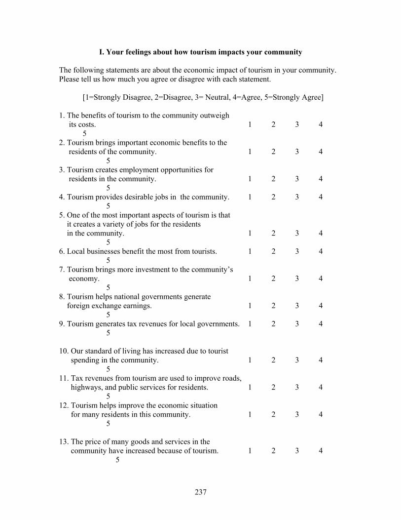
237
I. Your feelings about how tourism impacts your community The following statements are about the economic impact of tourism in your community. Please tell us how much you agree or disagree with each statement.
[1=Strongly Disagree, 2=Disagree, 3= Neutral, 4=Agree, 5=Strongly Agree] 1. The benefits of tourism to the community outweigh its costs. 1 2 3 4 5 2. Tourism brings important economic benefits to the residents of the community. 1 2 3 4
5 3. Tourism creates employment opportunities for residents in the community. 1 2 3 4
5 4. Tourism provides desirable jobs in the community. 1 2 3 4
5 5. One of the most important aspects of tourism is that it creates a variety of jobs for the residents in the community. 1 2 3 4
5 6. Local businesses benefit the most from tourists. 1 2 3 4
5 7. Tourism brings more investment to the community’s economy. 1 2 3 4
5 8. Tourism helps national governments generate foreign exchange earnings. 1 2 3 4
5 9. Tourism generates tax revenues for local governments. 1 2 3 4
5 10. Our standard of living has increased due to tourist spending in the community. 1 2 3 4
5 11. Tax revenues from tourism are used to improve roads, highways, and public services for residents. 1 2 3 4
5 12. Tourism helps improve the economic situation for many residents in this community. 1 2 3 4
5 13. The price of many goods and services in the community have increased because of tourism. 1 2 3 4
5

238
14. Real estate prices in the community have increased because of tourism. 1 2 3 4
5 15. The cost of living in the community has increased because of tourism. 1 2 3 4
5
The following statements are about the social impact of tourism in your community. Please tell us how much you agree or disagree with each statement.
[1=Strongly Disagree, 2=Disagree, 3= Neutral, 4=Agree, 5=Strongly Agree]
16. During the peak tourist season, I find it harder to get tickets for the theater, movies, concerts, or athletic events.1 2 3 4
5 17. Tourism has resulted in unpleasantly overcrowded hiking trails for local residents. 1 2 3 4
5 18. Tourism has resulted in unpleasantly overcrowded parks for local residents. 1 2 3 4
5 19. Tourism has resulted in unpleasantly overcrowded shopping places for local residents. 1 2 3 4
5 20. Tourism contributes social problems such as crime, drug use, prostitution, and so forth in the community. 1 2 3 4
5
21. Increased tourism provides more recreational opportunities for local residents. 1 2 3 4
5 22. Because of tourism, roads and other local services are well maintained. 1 2 3 4
5 23. Tourism is a major reason for the variety of entertainment in the community. 1 2 3 4
5 The following statements are about the cultural impact of tourism in your community. Please tell us how much you agree or disagree with each statement.
[1=Strongly Disagree, 2=Disagree, 3= Neutral, 4=Agree, 5=Strongly Agree]

239
24. Tourism has increased residents’ pride in the local culture in the community. 1 2 3 4
5 25. Tourism encourages a variety of cultural activities for local residents. 1 2 3 4
5 26. Tourism helps keep culture alive and helps maintain the ethnic identity of the local residents. 1 2 3 4
5 27. The commercial demand of tourists causes changes in the style and forms of traditional arts and crafts. 1 2 3 4
5 28. Tourism encourages residents to imitate the behavior of the tourists and relinquish cultural traditions. 1 2 3 4
5 29. Tourism causes the disruption of traditional cultural behavior patterns in local residents. 1 2 3 4
5 30. Meeting tourists from all over the world is definitely a life enriching experience. 1 2 3 4
5 31. The cultural exchange between residents and tourists is valuable for the residents. 1 2 3 4
5 32. The cultural exchange between residents and tourists is pleasant for the residents. 1 2 3 4
5 33. I would like to meet tourists from as many countries as possible in order to learn about their cultures. 1 2 3 4
5 The following statements are about the environmental impact of tourism in your
community. Please tell us how much you agree or disagree with each statement.
[1=Strongly Disagree, 2=Disagree, 3= Neutral, 4=Agree, 5=Strongly Agree] 34. Tourism causes environmental pollution. 1 2 3 4
5 35. Tourism produces noise. 1 2 3 4
5 36. Tourism produces littering. 1 2 3 4
5 37. Tourism produces congestion. 1 2 3 4
5

240
38. Tourist activities like boating produce serious water pollution in lakes, bays, or the ocean. 1 2 3 4
5 39. Tourism produces large quantities of waste products. 1 2 3 4
5 40. Hotels, airlines, attractions, and other related tourism businesses that serve tourists throw away tons of garbage. 1 2 3 4
5 41. Tourists’ littering destroys the beauty of the landscape. 1 2 3 4
5 42. Tourism has contributed to the preservation of the natural environment and the protection of the wildlife in the community. 1 2 3 4
5 43. Tourism has improved the ecological environment of the community in many ways. 1 2 3 4
5 44. Tourism does not contribute to the negative effect of vegetation and loss of meadows and green space. 1 2 3 4
5
II. Your feelings about life
The following statements are about your satisfaction in various living conditions. Please tell us how satisfied you are with each condition.
[1=Very Unsatisfied, 2= Unsatisfied, 3= Neutral, 4= Satisfied, 5=Very Satisfied] 1. Your income at your current job 1 2 3 4
5 2. The economic security of your job 1 2 3 4
5 3. Your family income 1 2 3 4
5 4. The pay and fringe benefits you receive 1 2 3 4
5 5. Your real estate taxes 1 2 3 4
5 6. The cost of living in your community 1 2 3 4
5 7. The cost of basic necessities such as food,

241
housing, and clothing 1 2 3 4 5
8. The conditions of the community environment (air, water, land) 1 2 3 4
5 9. The service you get in this community 1 2 3 4
5 10. The facilities you get in this community 1 2 3 4
5 11. The people who live in this community 1 2 3 4
5 12. Your spare time 1 2 3 4
5 13. Leisure activities in your community 1 2 3 4
5 14. The influx of tourists from all over the world into your community. 1 2 3 4
5 The following statements are about your satisfaction with life. Please tell us how much you agree or disagree with each statement.
[1=Strongly Disagree, 2=Disagree, 3= Neutral, 4=Agree, 5=Strongly Agree] 15. I am very satisfied with the availability of religious services in my community. 1 2 3 4
5 16. I am particularly happy with the way we preserve culture in my community. 1 2 3 4
5 17. I feel I extend my cultural outlook when I talk with tourists. 1 2 3 4
5 18. I always drink bottled or filtered water because I think the water is not clean. 1 2 3 4
5 19. When I see garbage left on the ground from the tourists, I don’t feel good about tourism. 1 2 3 4
5 20. Environmental pollution threatens public safety and causes health hazards. 1 2 3 4
5

242
The following statements are about your satisfaction with health and safety conditions. Please tell us how satisfied you are with each categories. [1=Very Unsatisfied, 2= Unsatisfied, 3= Neutral, 4= Satisfied, 5=Very Satisfied ] 21. Your health 1 2 3 4 5 22. Air quality in your area 1 2 3 4 5 23. Water quality in your area 1 2 3 4 5 24. Your leisure life 1 2 3 4 5 25. Your cultural life 1 2 3 4 5 26. Your social status 1 2 3 4 5 27. Your spiritual life 1 2 3 4 5 28. Your home life 1 2 3 4 5 29. Your community life 1 2 3 4 5 30. Environmental cleanness in your area 1 2 3 4 5 31. Accident and crime rates in your community 1 2 3 4 5 32. Safety and security in your community 1 2 3 4 5 33. Your life as a whole 1 2 3 4 5 34. The way you are spending your life 1 2 3 4
5
35. Which of the following statements best fits how you feel? (Check only one)
a. My life is much worse than most other people’s. b. My life is somewhat worse than most other people’s. c. My life is about the same as most other people. d. My life is somewhat better than most other people’s. e. My life is much better than most other people’s.
III. General information about tourism
1. The following are stages of tourism development from beginning, growth, and maturity to end. How do you rate the tourism development in your community?

243
[1] Beginning stage [2] Growth stage [3] Maturity stage [4] Decline stage
2. How long have you lived in the present community? ___________________
IV. About you 1. In what year were you born? _____________ 2. Gender: Male _________ Female ________ 3. Ethnic group: _______ Caucasian ________ Hispanic _______ African-American ________ Asian
_______ Other 4. Which of the following best describes your household? (check only one) _____ Single adult living alone or with other single adults _____ Single adult living with children or dependents _____ Married couple living without children or dependents at home _____ Married couple living with children or dependents at home 5. Including yourself, how many people make up your household? _______ 6. What was the last year of school you completed? (circle one) Grade school High School College Graduate School 1 2 3 4 5 6 7 8 9 10 11 12 F S J S Master Ph.D./Professional 7. Which of the following best describes your and your spouse’s present employment situation? Self Spouse (if applicable) Student _____ ______ Homemaker _____ ______ Unemployed _____ ______ Retired _____ ______ Professional/Technical _____ ______ Executive/ administrator _____ ______ Middle management _____ ______ Sales/marketing _____ ______ Clerical or service _____ ______

244
Tradesman/mechanic operator _____ ______ Self employed/ Business owner _____ ______ Government/military _____ ______ Educator _____ ______ Other (specify) _____ ______ 8. If employed outside the house, is your work (circle one) Full time _____ Part time _____ None _______ 9. How much of the income of the company you work for (or business you own) comes from the tourist trade? (circle one)
[1] None [2] A little [3] Some [4] A lot [5] Almost all 10. What part of your current household income comes from the money spent by the visitors to your community? Approximately _________________ % 11. What is your approximate household income before taxes?
_____ $20,000 or less _____ $ 60,001 - $ 80,000 _____ $20,001 - $40,000 _____ $ 80,001 - $ 100,000 _____ $40,001 - $60,000 _____ Over $100,000
Thank you for the filling out the survey. Please go back and check that you have responded to all survey questions. By completing this questionnaire, you will be included in a drawing for four 25$ cash awards. To be included for the drawing, please type or print your name and address in this box. Winner will be notified by phone in order to verify mailing address for awards. Name: Address: Tel:

245
Appendix B: Reminder postcard Dear Community residents, May 30, 2002 Recently, a questionnaire was sent to you from Virginia Tech asking about your assessment about the tourism impacts. If you have already filled out and returned the questionnaire, we really appreciate it! If the questionnaire has become lost or misplaced, we would be more than happy to send you another copy. We appreciate the time and effort that take the complete questionnaire. Your responses are very important in Virginia Tech’s effort to continue to provide the community residents with pertinent and valuable research and technical assistance. If you have any question or comment, please contact Kyungmi Kim at Virginia Tech by telephone (540) 961-7213 or by e-mail at [email protected] Sincerely, Kyungmi Kim, ABD Principal Investigator Hospitality and Tourism Management Box 850 Virginia Tech Blacksburg, VA 24061
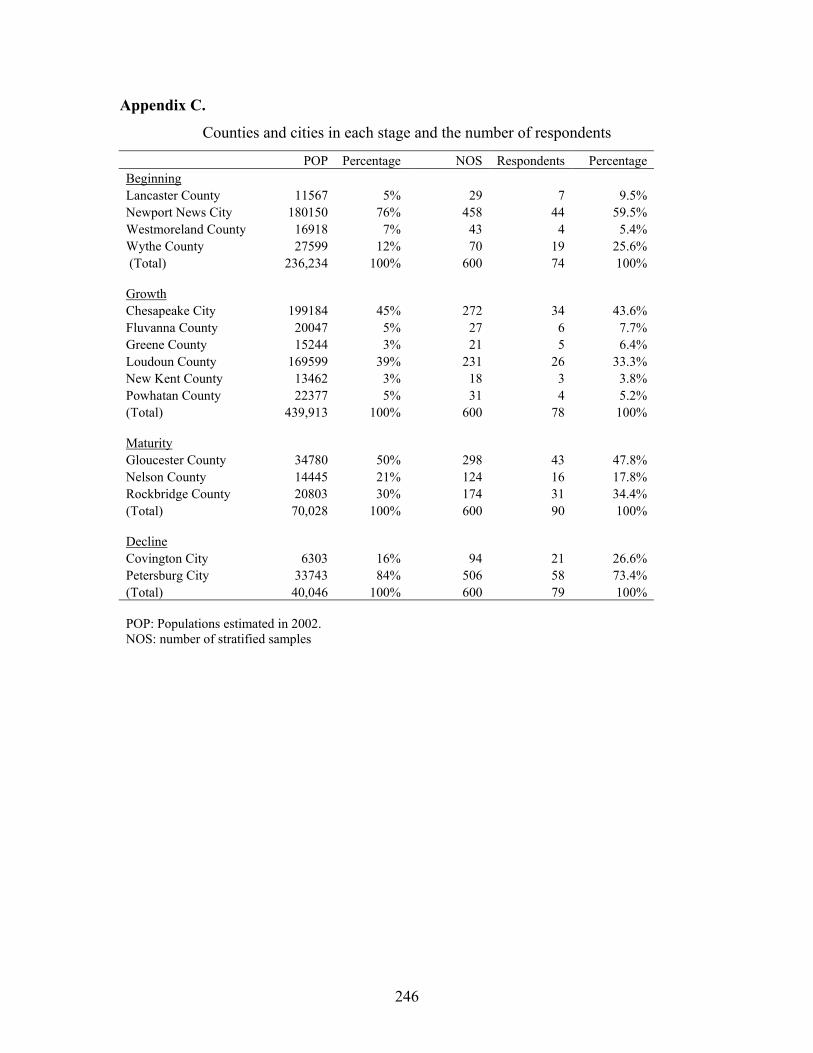
246
Appendix C.
Counties and cities in each stage and the number of respondents
POP Percentage NOS Respondents Percentage Beginning Lancaster County 11567 5% 29 7 9.5% Newport News City 180150 76% 458 44 59.5% Westmoreland County 16918 7% 43 4 5.4% Wythe County 27599 12% 70 19 25.6% (Total) 236,234 100% 600 74 100% Growth Chesapeake City 199184 45% 272 34 43.6% Fluvanna County 20047 5% 27 6 7.7% Greene County 15244 3% 21 5 6.4% Loudoun County 169599 39% 231 26 33.3% New Kent County 13462 3% 18 3 3.8% Powhatan County 22377 5% 31 4 5.2% (Total) 439,913 100% 600 78 100% Maturity Gloucester County 34780 50% 298 43 47.8% Nelson County 14445 21% 124 16 17.8% Rockbridge County 20803 30% 174 31 34.4% (Total) 70,028 100% 600 90 100% Decline Covington City 6303 16% 94 21 26.6% Petersburg City 33743 84% 506 58 73.4% (Total) 40,046 100% 600 79 100% POP: Populations estimated in 2002. NOS: number of stratified samples
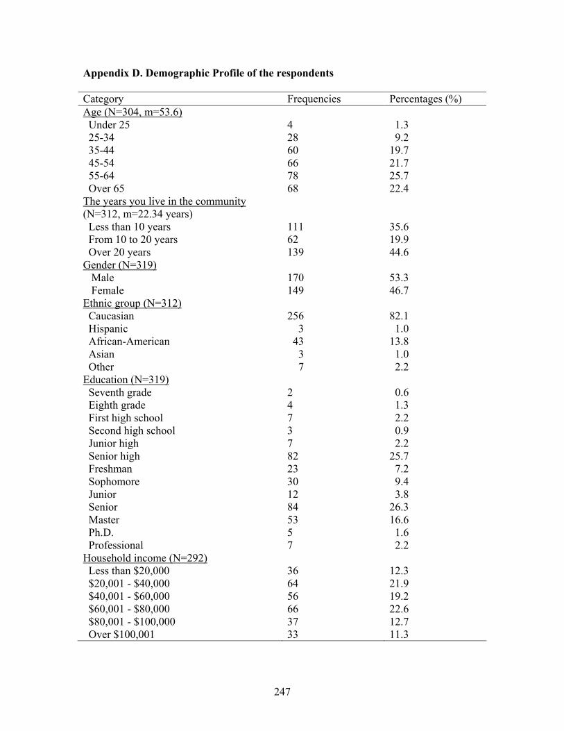
Appendix D. Demographic Profile of the respondents Category Frequencies Percentages (%) Age (N=304, m=53.6) Under 25 25-34 35-44 45-54 55-64 Over 65
4 28 60 66 78 68
1.3 9.2 19.7 21.7 25.7 22.4
The years you live in the community (N=312, m=22.34 years) Less than 10 years From 10 to 20 years Over 20 years�
111 62 139
35.6 19.9 44.6
Gender (N=319) Male Female
170 149
53.3 46.7
Ethnic group (N=312) Caucasian Hispanic African-American Asian Other
256 3 43 3 7
82.1 1.0 13.8 1.0 2.2
Education (N=319) Seventh grade Eighth grade First high school Second high school Junior high Senior high Freshman Sophomore Junior Senior Master Ph.D. Professional
2 4 7 3 7 82 23 30 12 84 53 5 7
0.6 1.3 2.2 0.9 2.2 25.7 7.2 9.4 3.8 26.3 16.6 1.6 2.2
Household income (N=292) Less than $20,000 $20,001 - $40,000 $40,001 - $60,000 $60,001 - $80,000 $80,001 - $100,000 Over $100,001
36 64 56 66 37 33
12.3 21.9 19.2 22.6 12.7 11.3
247
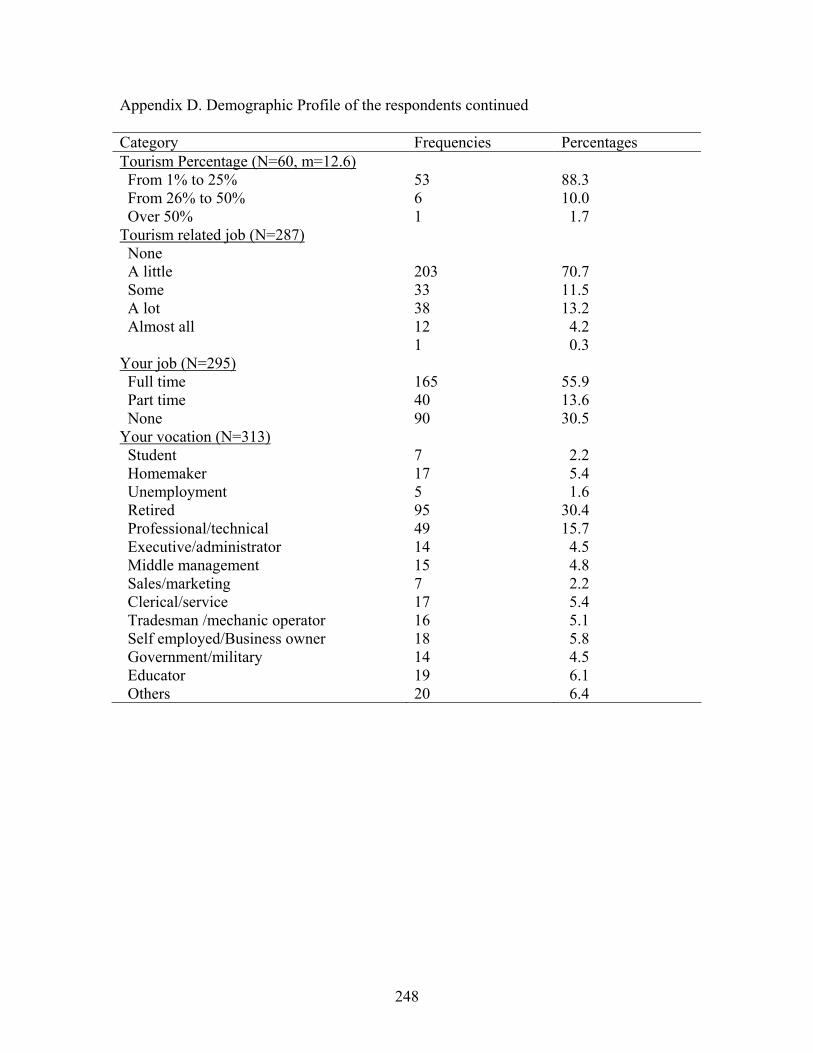
Appendix D. Demographic Profile of the respondents continued Category Frequencies Percentages Tourism Percentage (N=60, m=12.6) From 1% to 25% From 26% to 50% Over 50%
53 6 1
88.3 10.0 1.7
Tourism related job (N=287) None A little Some A lot Almost all
203 33 38 12 1
70.7 11.5 13.2 4.2 0.3
Your job (N=295) Full time Part time None
165 40 90
55.9 13.6 30.5
Your vocation (N=313) Student Homemaker Unemployment Retired Professional/technical Executive/administrator Middle management Sales/marketing Clerical/service Tradesman /mechanic operator Self employed/Business owner Government/military Educator Others
7 17 5 95 49 14 15 7 17 16 18 14 19 20
2.2 5.4 1.6 30.4 15.7 4.5 4.8 2.2 5.4 5.1 5.8 4.5 6.1 6.4
248

Appendix D. Demographic Profile of the respondents continued Category Frequencies Percentages Your spouse’s vocation (N=244) Student Homemaker Unemployment Retired Professional/technical Executive/administrator Middle management Sales/marketing Clerical/service Tradesman /mechanic operator Self employed/Business owner Government/military Educator Others
4 30 4 57 37 9 10 11 14 21 21 8 12 6
1.6 12.3 1.6 23.4 15.2 3.7 4.1 4.5 5.7 8.6 8.6 3.3 4.9 2.5
Household status (N=314) Single adult living alone or other single adults Single adult with children or other dependent Married couple living without children Married couple living with children
58 17 139 100
18.5 5.4 44.3 31.8
How many people in your household (n=310) 1.00 2.00 3.00 4.00 5.00 6.00
40 156 47 50 15 2
12.9 50.3 15.2 16.1 4.8 0.6
249
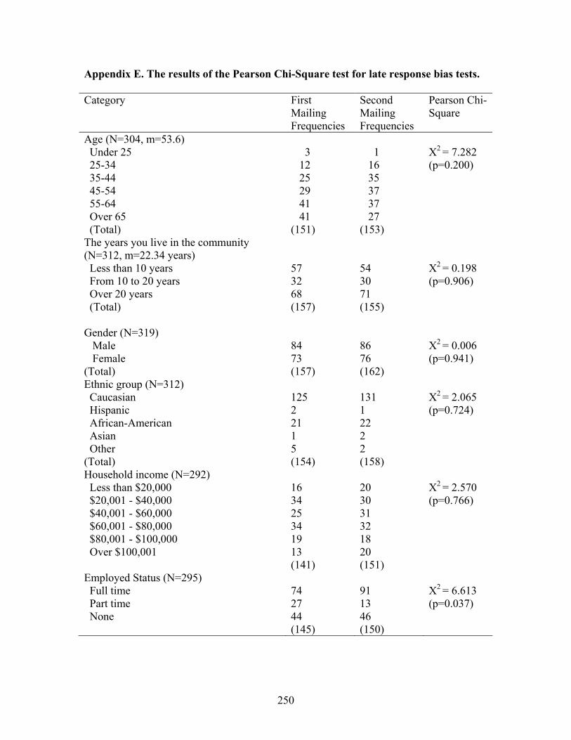
Appendix E. The results of the Pearson Chi-Square test for late response bias tests. Category First
Mailing Frequencies
Second Mailing Frequencies
Pearson Chi-Square
Age (N=304, m=53.6) Under 25 25-34 35-44 45-54 55-64 Over 65 (Total)
3 12 25 29 41 41 (151)
1 16 35 37 37 27 (153)
Χ2 = 7.282 (p=0.200)
The years you live in the community (N=312, m=22.34 years) Less than 10 years From 10 to 20 years Over 20 years (Total)
57 32 68 (157)
54 30 71 (155)
Χ2 = 0.198 (p=0.906)
Gender (N=319) Male Female (Total)
84 73 (157)
86 76 (162)
Χ2 = 0.006 (p=0.941)
Ethnic group (N=312) Caucasian Hispanic African-American Asian Other (Total)
125 2 21 1 5 (154)
131 1 22 2 2 (158)
Χ2 = 2.065 (p=0.724)
Household income (N=292) Less than $20,000 $20,001 - $40,000 $40,001 - $60,000 $60,001 - $80,000 $80,001 - $100,000 Over $100,001
16 34 25 34 19 13 (141)
20 30 31 32 18 20 (151)
Χ2 = 2.570 (p=0.766)
Employed Status (N=295) Full time Part time None
74 27 44 (145)
91 13 46 (150)
Χ2 = 6.613 (p=0.037)
250

Category First Mailing Frequencies
Second Mailing Frequencies
Pearson Chi-Square
Education (N=319) Seventh grade Eighth grade First high school Second high school Junior high Senior high Freshman Sophomore Junior Senior Master Ph.D. Professional
1 1 3 1 1 40 10 17 8 42 24 4 5 (157)
1 3 4 2 6 42 13 13 4 42 29 1 2 (162)
Χ2 = 10.836 (p=0.543)
Tourism Percentage (N=60, m=12.6) From 1% to 25% From 26% to 50% Over 50%
30 3 0 (33)
23 3 1 (27)
Χ2 = 1.338 (p=0.512)
Income from the tourist trade (N=287) None A little Some A lot Almost all
92 18 21 7 (138)
111 15 17 5 1 (149)
Χ2 = 3.389 (p=0.495)
Household status (N=314) Single adult living alone or other single adults Single adult with children or other dependent Married couple living without children Married couple living with children
27 9 72 49 (157)
31 8 67 51 (157)
Χ2 = 0.555 (p=0.907)
How many people in your household 1.00 2.00 3.00 4.00 5.00 6.00
21 82 22 22 7 0 (154)
19 74 25 28 8 2 (156)
Χ2 = 3.476 (p=0.627)
251
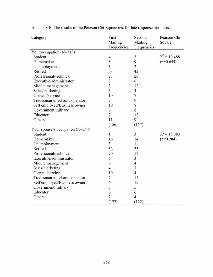
252
Appendix E. The results of the Pearson Chi-Square test for late response bias tests. Category First
Mailing Frequencies
Second Mailing Frequencies
Pearson Chi-Square
Your occupation (N=313) Student Homemaker Unemployment Retired Professional/technical Executive/administrator Middle management Sales/marketing Clerical/service Tradesman /mechanic operator Self employed/Business owner Government/military Educator Others
4 8 3 53 23 8 3 3 10 7 10 6 7 11 (156)
3 9 2 42 26 6 12 4 7 9 8 8 12 9 (157)
Χ2 = 10.488 (p=0.654)
Your spouse’s occupation (N=244) Student Homemaker Unemployment Retired Professional/technical Executive/administrator Middle management Sales/marketing Clerical/service Tradesman /mechanic operator Self employed/Business owner Government/military Educator Others
1 16 3 32 20 6 6 4 10 7 6 3 6 2 (122)
3 14 1 25 17 3 4 7 4 14 15 5 6 4 (122)
Χ2 = 15.383 (p=0.284)

253
Appendix F.
Individual items of the constructs with mean scores and standard deviation
1. Economic impact constructs and variables
Variables Mean SD Skew. Kurt. Employment opportunity
Provides desirable jobs Creates variety of jobs Creates employment opportunity Revenue from tourist for local business and government Brings more investment and spending Local government generates foreign exchange Generates tax revenues for local governments Local business benefits from tourism
Standard of living Standard of living increases Improve economic situation To improve roads, highways, and public services
Cost of living The cost of living in the community The price of goods and service increases Real estate prices in the community
3.52 3.56 4.01 3.59 3.31 3.90 3.83 2.99 3.14 2.99 3.11 3.21 3.21
1.046 .979 .897 .938 .854 .872 .941 1.042 1.025 1.016 .997 .985 1.033
-.661 -.868 -1.353 -.763 -.233 -1.125 -.858 -.160 -.476 -.319 .008 -.101 -.010
-.033 .385 2.251 .491 .476 1.725 .606 -.558 -.523 -.575 -.742 -.531 -.717
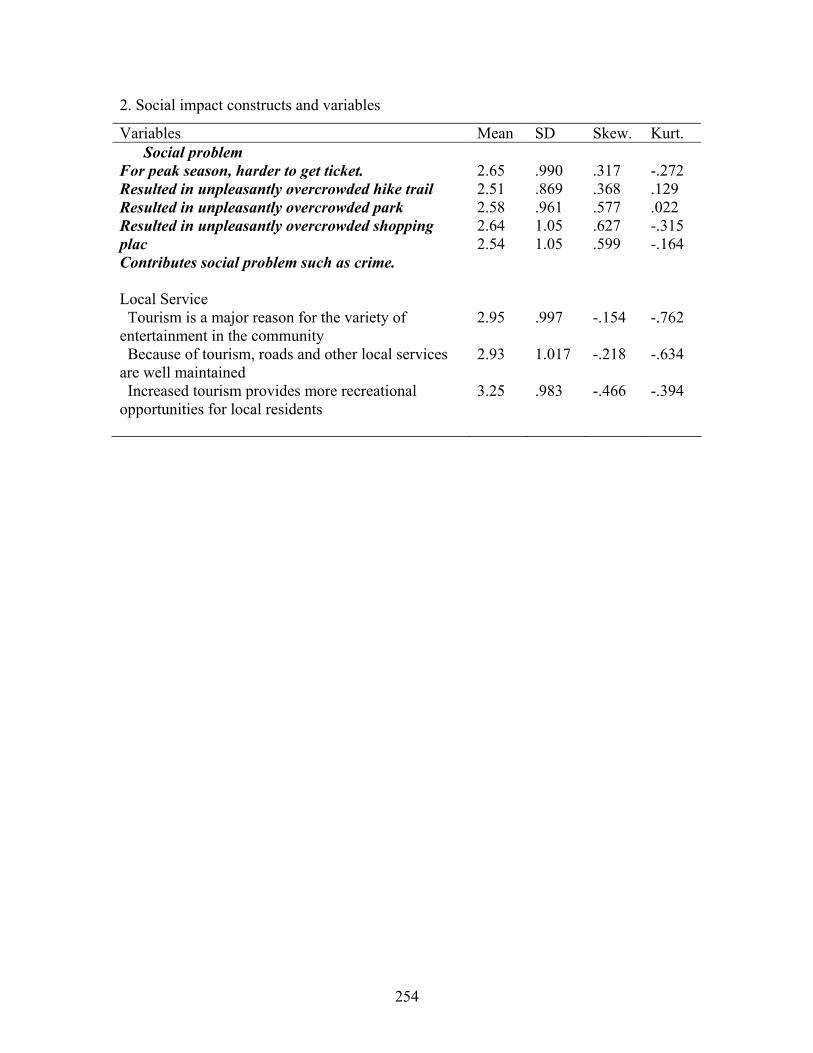
254
2. Social impact constructs and variables
Variables Mean SD Skew. Kurt. Social problem
For peak season, harder to get ticket. Resulted in unpleasantly overcrowded hike trail Resulted in unpleasantly overcrowded park Resulted in unpleasantly overcrowded shopping plac Contributes social problem such as crime. Local Service Tourism is a major reason for the variety of entertainment in the community Because of tourism, roads and other local services are well maintained Increased tourism provides more recreational opportunities for local residents
2.65 2.51 2.58 2.64 2.54 2.95 2.93 3.25
.990 .869 .961 1.05 1.05 .997 1.017 .983
.317 .368 .577 .627 .599 -.154 -.218 -.466
-.272 .129 .022 -.315 -.164 -.762 -.634 -.394
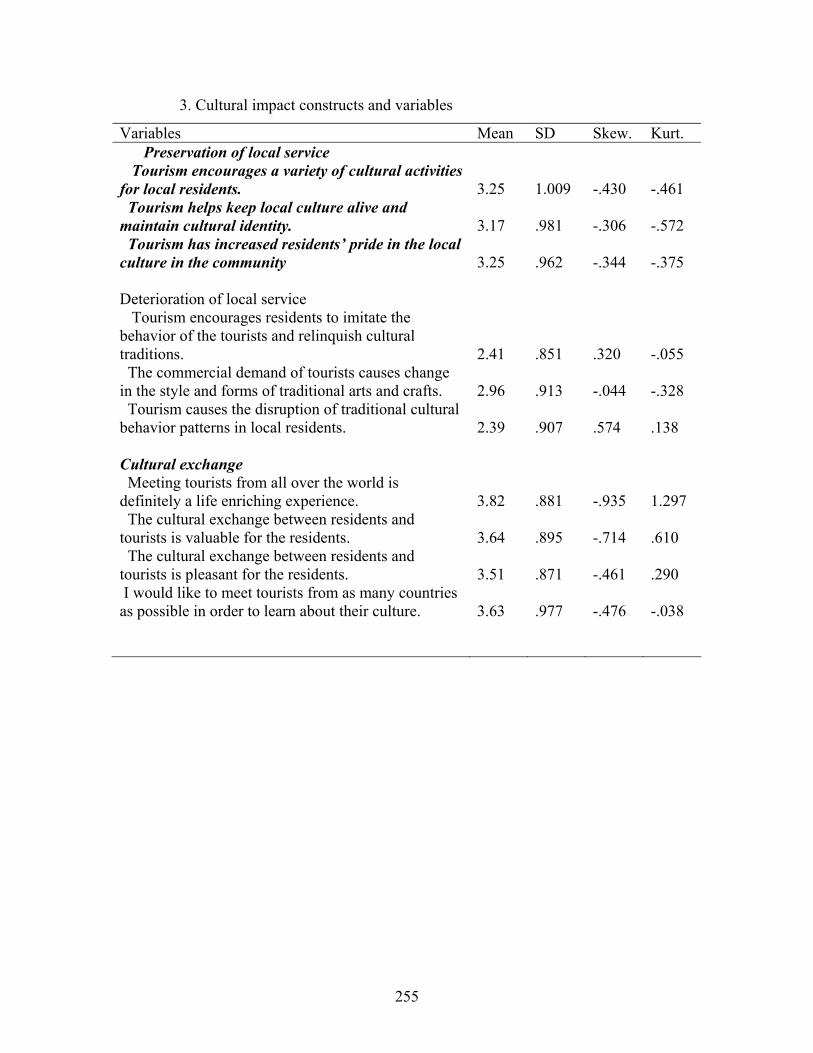
255
3. Cultural impact constructs and variables
Variables Mean SD Skew. Kurt. Preservation of local service
Tourism encourages a variety of cultural activities for local residents. Tourism helps keep local culture alive and maintain cultural identity. Tourism has increased residents’ pride in the local culture in the community Deterioration of local service Tourism encourages residents to imitate the behavior of the tourists and relinquish cultural traditions. The commercial demand of tourists causes change in the style and forms of traditional arts and crafts. Tourism causes the disruption of traditional cultural behavior patterns in local residents. Cultural exchange Meeting tourists from all over the world is definitely a life enriching experience. The cultural exchange between residents and tourists is valuable for the residents. The cultural exchange between residents and tourists is pleasant for the residents. I would like to meet tourists from as many countries as possible in order to learn about their culture.
3.25 3.17 3.25 2.41 2.96 2.39 3.82 3.64 3.51 3.63
1.009 .981 .962 .851 .913 .907 .881 .895 .871 .977
-.430 -.306 -.344 .320 -.044 .574 -.935 -.714 -.461 -.476
-.461 -.572 -.375 -.055 -.328 .138 1.297 .610 .290 -.038
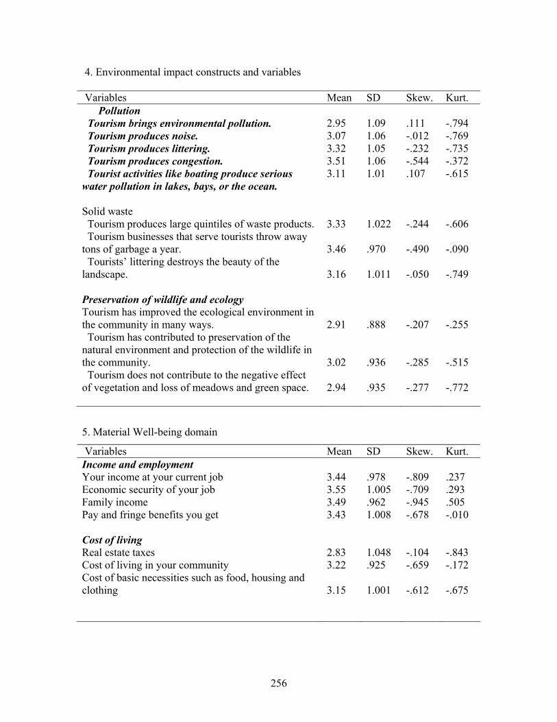
256
4. Environmental impact constructs and variables Variables Mean SD Skew. Kurt.
Pollution Tourism brings environmental pollution. Tourism produces noise. Tourism produces littering. Tourism produces congestion. Tourist activities like boating produce serious water pollution in lakes, bays, or the ocean. Solid waste Tourism produces large quintiles of waste products. Tourism businesses that serve tourists throw away tons of garbage a year. Tourists’ littering destroys the beauty of the landscape. Preservation of wildlife and ecology Tourism has improved the ecological environment in the community in many ways. Tourism has contributed to preservation of the natural environment and protection of the wildlife in the community. Tourism does not contribute to the negative effect of vegetation and loss of meadows and green space.
2.95 3.07 3.32 3.51 3.11 3.33 3.46 3.16 2.91 3.02 2.94
1.09 1.06 1.05 1.06 1.01 1.022 .970 1.011 .888 .936 .935
.111 -.012 -.232 -.544 .107 -.244 -.490 -.050 -.207 -.285 -.277
-.794 -.769 -.735 -.372 -.615 -.606 -.090 -.749 -.255 -.515 -.772
5. Material Well-being domain
Variables Mean SD Skew. Kurt. Income and employment Your income at your current job Economic security of your job Family income Pay and fringe benefits you get Cost of living Real estate taxes Cost of living in your community Cost of basic necessities such as food, housing and clothing
3.44 3.55 3.49 3.43 2.83 3.22 3.15
.978 1.005 .962 1.008 1.048 .925 1.001
-.809 -.709 -.945 -.678 -.104 -.659 -.612
.237 .293 .505 -.010 -.843 -.172 -.675
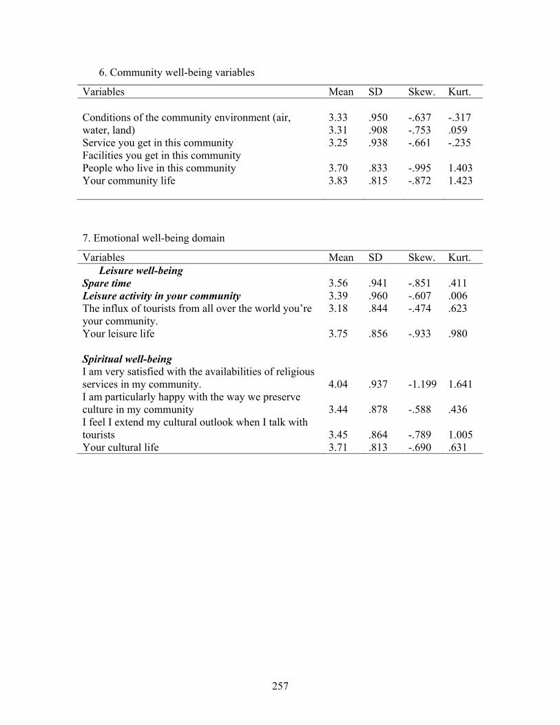
257
6. Community well-being variables
Variables Mean SD Skew. Kurt. Conditions of the community environment (air, water, land) Service you get in this community Facilities you get in this community People who live in this community Your community life
3.33 3.31 3.25 3.70 3.83�
.950 .908 .938 .833 .815�
-.637 -.753 -.661 -.995 -.872
-.317 .059 -.235 1.403 1.423�
7. Emotional well-being domain
Variables Mean SD Skew. Kurt. Leisure well-being
Spare time Leisure activity in your community The influx of tourists from all over the world you’re your community. Your leisure life Spiritual well-being I am very satisfied with the availabilities of religious services in my community. I am particularly happy with the way we preserve culture in my community I feel I extend my cultural outlook when I talk with tourists Your cultural life
3.56 3.39 3.18 3.75 4.04 3.44 3.45 3.71�
.941 .960 .844 .856 .937 .878 .864 .813�
-.851 -.607 -.474 -.933 -1.199 -.588 -.789 -.690
.411 .006 .623 .980 1.641 .436 1.005 .631�
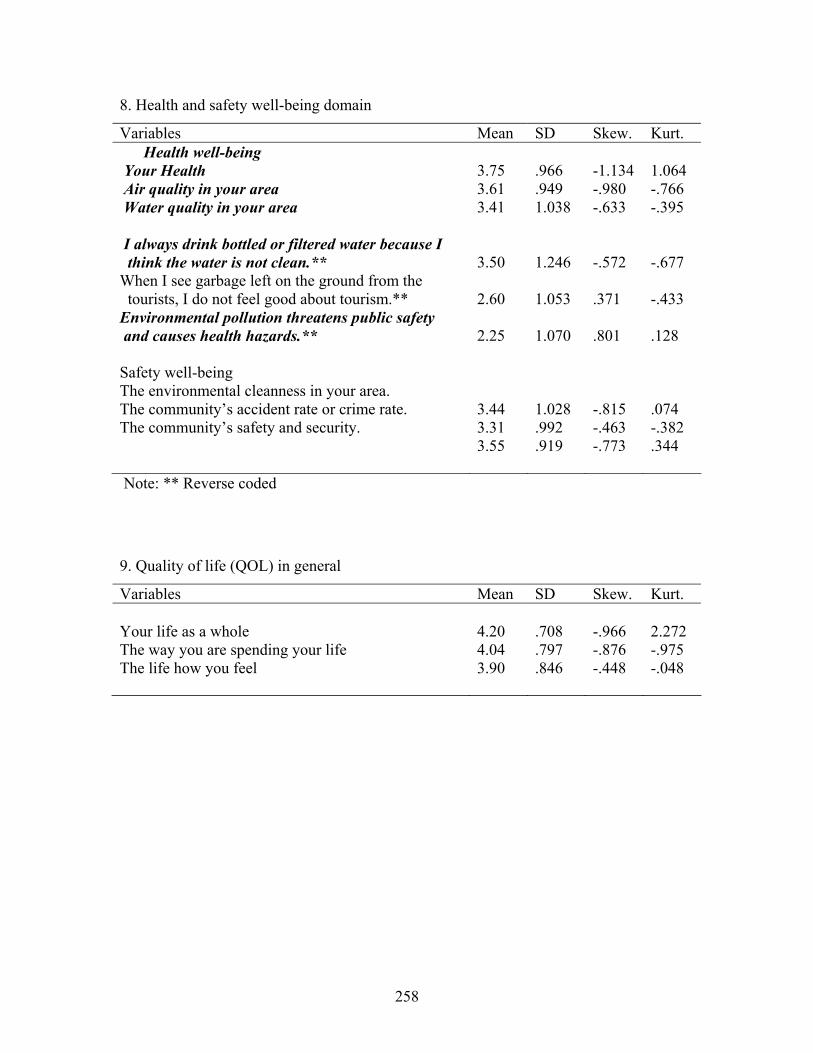
258
8. Health and safety well-being domain
Variables Mean SD Skew. Kurt. Health well-being
Your Health Air quality in your area Water quality in your area I always drink bottled or filtered water because I think the water is not clean.** When I see garbage left on the ground from the tourists, I do not feel good about tourism.** Environmental pollution threatens public safety and causes health hazards.** Safety well-being The environmental cleanness in your area. The community’s accident rate or crime rate. The community’s safety and security.
3.75 3.61 3.41 3.50 2.60 2.25 3.44 3.31 3.55
.966 .949 1.038 1.246 1.053 1.070 1.028 .992 .919
-1.134 -.980 -.633 -.572 .371 .801 -.815 -.463 -.773
1.064 -.766 -.395 -.677 -.433 .128 .074 -.382 .344
Note: ** Reverse coded
9. Quality of life (QOL) in general
Variables Mean SD Skew. Kurt. Your life as a whole The way you are spending your life The life how you feel
4.20 4.04 3.90
.708 .797 .846
-.966 -.876 -.448
2.272 -.975 -.048

259
APPENDIX G. The procedure of selecting the number of indicators 1. The cutting value used to select the indicators and constructs Number of indicators overall fit Each loading Degrees of Freedom Least Squares Chi-Square
Less than DF*3
P >0.05 Sample size >100 RMSEA Close to 0.06
No – loading, Should be P<0.05
Standized residual should be less than 2.56
SRMR Close to 0.08 GFI Close to 0.95 AGFI Close to 0.95 PGFI IFI Close to 0.95 NNFI Close to 0.95
Error variance should not be greater than .5
Modification indices should be less than 3.89 on other latent variables
CFI Close to 0.95 RNI Close to 0.95 Critical N (CN) >=200 2. Economic impact of tourism construct Number of indicators RLG (4) RLG & EO RLG*SL RLG*CL Degrees of Freedom 2 P=0.74 13 P=0.00 13 P=0.85 13 P=0.095 Least Squares Chi-Square
0.59 46.33 7.94 19.58
RMSEA 0.0 0.090 0.0 0.040 SRMR 0.0072 0.034 0.014 0.047 GFI 1.00 0.96 0.99 0.98 AGFI 1.00 0.91 0.98 0.96 PGFI 0.2 0.45 0.46 0.46 NFI 1.00 0.96 0.99 0.97 NNFI 1.00 0.95 1.01 0.98 PNFI 0.33 0.59 0.61 0.60 CFI 1.00 0.97 1.00 0.99 IFI 1.00 0.97 1.01 0.99 RFI 0.99 0.93 0.99 0.96 Critical N (CN) 4897.37 196.47 1096.44 443.94
Note: EO-Employment opportunity, RLG-Revenue from tourist for local business and government, SL-Standard of living, CL-Cost of living
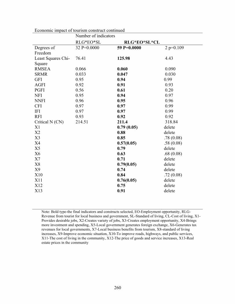
260
Economic impact of tourism construct continued Number of indicators RLG*EO*SL RLG*EO*SL*CL Degrees of Freedom
32 P=0.0000 59 P=0.0000 2 p=0.109
Least Squares Chi-Square
76.41 125.98 4.43
RMSEA 0.066 0.060 0.090 SRMR 0.033 0.047 0.030 GFI 0.95 0.94 0.99 AGFI 0.92 0.91 0.93 PGFI 0.56 0.61 0.20 NFI 0.95 0.94 0.97 NNFI 0.96 0.95 0.96 CFI 0.97 0.97 0.99 IFI 0.97 0.97 0.99 RFI 0.93 0.92 0.92 Critical N (CN) 214.51 211.4 318.84 X1 0.79 (0.05) delete X2 0.88 delete X3 0.85 .78 (0.08) X4 0.57(0.05) .58 (0.08) X5 0.79 delete X6 0.63 .68 (0.08) X7 0.71 delete X8 0.79(0.05) delete X9 0.74 delete X10 0.84 .72 (0.08) X11 0.76(0.05) delete X12 0.75 delete X13 0.91 delete
Note: Bold type-the final indicators and constructs selected, EO-Employment opportunity, RLG-Revenue from tourist for local business and government, SL-Standard of living, CL-Cost of living, X1-Provides desirable jobs, X2-Creates variety of jobs, X3-Creates employment opportunity, X4-Brings more investment and spending, X5-Local government generates foreign exchange, X6-Generates tax revenues for local governments, X7-Local business benefits from tourism, X8-standard of living increases, X9-Improve economic situation, X10-To improve roads, highways, and public services, X11-The cost of living in the community, X12-The price of goods and service increases, X13-Real estate prices in the community
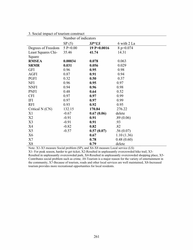
261
3. Social impact of tourism construct Number of indicators SP (5) SP*LS 6 with 2 La Degrees of Freedom 5 P=0.00 19 P=0.0016 8 p=0.074 Least Squares Chi-Square
35.46 41.74 14.31
RMSEA 0.00034 0.078 0.063 SRMR 0.031 0.056 0.029 GFI 0.96 0.95 0.98 AGFI 0.87 0.91 0.94 PGFI 0.32 0.50 0.37 NFI 0.96 0.95 0.97 NNFI 0.94 0.96 0.98 PNFI 0.48 0.64 0.52 CFI 0.97 0.97 0.99 IFI 0.97 0.97 0.99 RFI 0.93 0.92 0.95 Critical N (CN) 132.15 170.84 276.22 X1 -0.67 0.67 (0.06) delete X2 -0.91 0.91 .89 (0.06) X3 -0.91 0.91 .93 X4 -0.82 0.82 .82 X5 -0.57 0.57 (0.07) .56 (0.07) X6 0.67 1.10 (1.36) X7 0.78 0.48 (0.60) X8 0.79 delete Note: X1-X5 measure Social problem (SP), and X6-X8 measure Local service (LS) X1- For peak season, harder to get ticket, X2-Resulted in unpleasantly overcrowded hike trail, X3- Resulted in unpleasantly overcrowded park, X4-Resulted in unpleasantly overcrowded shopping place, X5-Contributes social problem such as crime, X6-Tourism is a major reason for the variety of entertainment in the community, X7-Because of tourism, roads and other local services are well maintained, X8-Increased tourism provides more recreational opportunities for local residents.
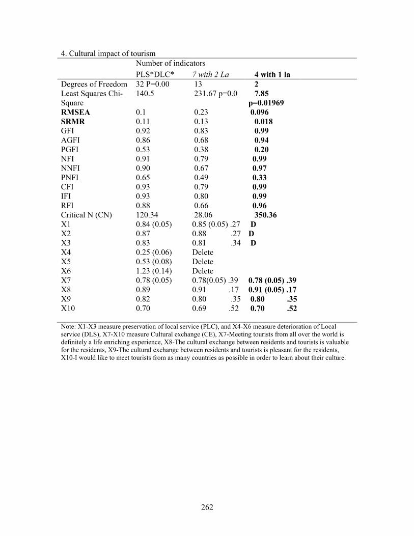
262
4. Cultural impact of tourism Number of indicators PLS*DLC* 7 with 2 La 4 with 1 la Degrees of Freedom 32 P=0.00 13 2 Least Squares Chi-Square
140.5 231.67 p=0.0 7.85 p=0.01969
RMSEA 0.1 0.23 0.096 SRMR 0.11 0.13 0.018 GFI 0.92 0.83 0.99 AGFI 0.86 0.68 0.94 PGFI 0.53 0.38 0.20 NFI 0.91 0.79 0.99 NNFI 0.90 0.67 0.97 PNFI 0.65 0.49 0.33 CFI 0.93 0.79 0.99 IFI 0.93 0.80 0.99 RFI 0.88 0.66 0.96 Critical N (CN) 120.34 28.06 350.36 X1 0.84 (0.05) 0.85 (0.05) .27 D X2 0.87 0.88 .27 D X3 0.83 0.81 .34 D X4 0.25 (0.06) Delete X5 0.53 (0.08) Delete X6 1.23 (0.14) Delete X7 0.78 (0.05) 0.78(0.05) .39 0.78 (0.05) .39 X8 0.89 0.91 .17 0.91 (0.05) .17 X9 0.82 0.80 .35 0.80 .35 X10 0.70 0.69 .52 0.70 .52 Note: X1-X3 measure preservation of local service (PLC), and X4-X6 measure deterioration of Local service (DLS), X7-X10 measure Cultural exchange (CE), X7-Meeting tourists from all over the world is definitely a life enriching experience, X8-The cultural exchange between residents and tourists is valuable for the residents, X9-The cultural exchange between residents and tourists is pleasant for the residents, X10-I would like to meet tourists from as many countries as possible in order to learn about their culture.

263
5. Environmental impact of tourism Number of indicators 11 with 3 LA 10 with 3La 9 with 3 La 8 with 3 LA Degrees of Freedom 41 P=0.00 32 P=0.00005 24 p=0.00024 17 p=0.00397 Least Squares Chi-Square
99.51 73.06 55.81 36.47
RMSEA 0.085 0.080 0.082 0.076 SRMR 0.083 0.038 0.034 0.030 GFI 0.92 0.93 0.94 0.96 AGFI 0.87 0.88 0.89 0.91 PGFI 0.57 0.54 0.50 0.45 NFI 0.93 0.95 0.95 0.96 NNFI 0.94 0.96 0.96 0.95 PNFI 0.69 0.67 0.63 0.58 CFI 0.96 0.97 0.97 0.97 IFI 0.96 0.97 0.97 0.97 RFI 0.91 0.93 0.93 0.93 Critical N (CN) 133.05 152.88 150.03 150.03 X1 0.85 (0.06) .28 0.85 (0.06) .28 0.86 (0.06) .27 0.88 (0.06) .22 X2 0.90 (0.06) .18 0.90 .18 0.92 .16 0.92 .16X3 0.87 .24 0.87 .24 0.86 .26 0.85 .28X4 0.77 .40 0.77 .40 0.78 .40 D X5 0.76 .42 0.76 .42 D D X6 0.91 .17 0.91 .17 0.90 (0.06) .19 0.88 .22 X7 0.74 .46 0.74 .46 0.75 (0.07) .44 0.77 .41 X8 0.62 (0.07) .62 0.62 (0.07) .62 0.62 .62 0.62 (0.07) .61 X9 0.84 (0.08) .30 0.83 (0.13) .30 0.84 (0.14) .30 0.84 (0.15) .30 X10 0.88 (0.08) .23 0.89 (0.14) .21 0.89 (0.15) .22 0.89 (0.15) .22 X11 0.42 (0.07) .82 delete D D
Note: X1-5 measure Pollution(P), X1-tourism brings environmental pollution, X2-Tourism produces noise, X3-Tourism produces littering, X4-Tourism produces congestion, X5-Tourist activities like boating produce serious water pollution in lakes, bays, or the ocean, X6-8 measure Solid waste (SW), X6-Tourism produces large quintiles of waste products, X7-Tourism businesses that serve tourists throw away tons of garbage a year, X8-Tourists’ littering destroys the beauty of the landscape, X9-11 measure Preservation of wildlife and ecology (PWE), X9-Tourism has improved the ecological environment in the community in many ways, X10-Tourism has contributed to preservation of the natural environment and protection of the wildlife in the community, X11-Tourism does not contribute to the negative effect of vegetation and loss of meadows and green space.
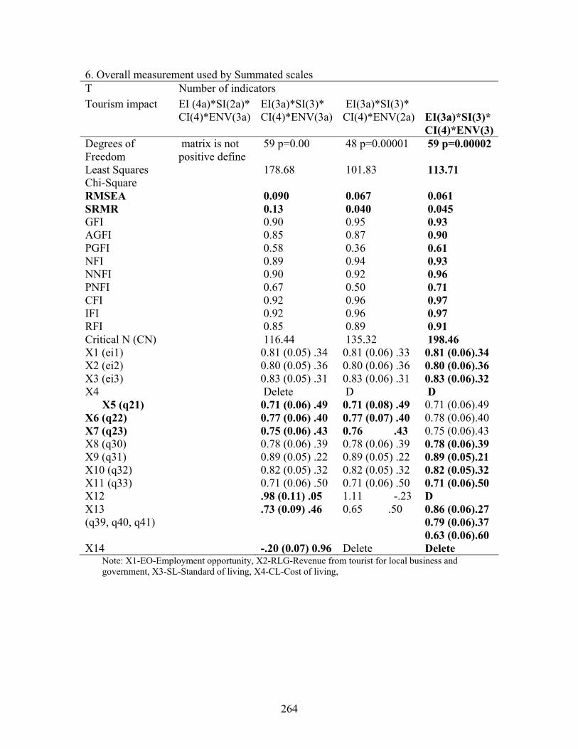
264
6. Overall measurement used by Summated scales T Number of indicators Tourism impact EI (4a)*SI(2a)*
CI(4)*ENV(3a)EI(3a)*SI(3)* CI(4)*ENV(3a)
EI(3a)*SI(3)* CI(4)*ENV(2a)
EI(3a)*SI(3)* CI(4)*ENV(3)
Degrees of Freedom
matrix is not positive define
59 p=0.00 48 p=0.00001 59 p=0.00002
Least Squares Chi-Square
178.68 101.83 113.71
RMSEA 0.090 0.067 0.061 SRMR 0.13 0.040 0.045 GFI 0.90 0.95 0.93 AGFI 0.85 0.87 0.90 PGFI 0.58 0.36 0.61 NFI 0.89 0.94 0.93 NNFI 0.90 0.92 0.96 PNFI 0.67 0.50 0.71 CFI 0.92 0.96 0.97 IFI 0.92 0.96 0.97 RFI 0.85 0.89 0.91 Critical N (CN) 116.44 135.32 198.46 X1 (ei1) 0.81 (0.05) .34 0.81 (0.06) .33 0.81 (0.06).34 X2 (ei2) 0.80 (0.05) .36 0.80 (0.06) .36 0.80 (0.06).36 X3 (ei3) 0.83 (0.05) .31 0.83 (0.06) .31 0.83 (0.06).32 X4 Delete D D
X5 (q21) 0.71 (0.06) .49 0.71 (0.08) .49 0.71 (0.06).49 X6 (q22) 0.77 (0.06) .40 0.77 (0.07) .40 0.78 (0.06).40 X7 (q23) 0.75 (0.06) .43 0.76 .43 0.75 (0.06).43 X8 (q30) 0.78 (0.06) .39 0.78 (0.06) .39 0.78 (0.06).39 X9 (q31) 0.89 (0.05) .22 0.89 (0.05) .22 0.89 (0.05).21 X10 (q32) 0.82 (0.05) .32 0.82 (0.05) .32 0.82 (0.05).32 X11 (q33) 0.71 (0.06) .50 0.71 (0.06) .50 0.71 (0.06).50 X12 .98 (0.11) .05 1.11 -.23 D X13 (q39, q40, q41)
.73 (0.09) .46 0.65 .50 0.86 (0.06).27 0.79 (0.06).37 0.63 (0.06).60
X14 -.20 (0.07) 0.96 Delete Delete Note: X1-EO-Employment opportunity, X2-RLG-Revenue from tourist for local business and government, X3-SL-Standard of living, X4-CL-Cost of living,
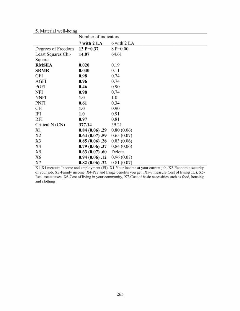
265
5. Material well-being Number of indicators 7 with 2 LA 6 with 2 LA Degrees of Freedom 13 P=0.37 8 P=0.00 Least Squares Chi-Square
14.07 64.61
RMSEA 0.020 0.19 SRMR 0.040 0.11 GFI 0.98 0.74 AGFI 0.96 0.74 PGFI 0.46 0.90 NFI 0.98 0.74 NNFI 1.0 1.0 PNFI 0.61 0.34 CFI 1.0 0.90 IFI 1.0 0.91 RFI 0.97 0.81 Critical N (CN) 377.14 59.21 X1 0.84 (0.06) .29 0.80 (0.06) X2 0.64 (0.07) .59 0.65 (0.07) X3 0.85 (0.06) .28 0.83 (0.06) X4 0.79 (0.06) .37 0.84 (0.06) X5 0.63 (0.07) .60 Delete X6 0.94 (0.06) .12 0.96 (0.07) X7 0.82 (0.06) .32 0.81 (0.07) X1-X4 measure Income and employment (EI), X1-Your income at your current job, X2-Economic security of your job, X3-Family income, X4-Pay and fringe benefits you get , X5-7 measure Cost of living(CL), X5-Real estate taxes, X6-Cost of living in your community, X7-Cost of basic necessities such as food, housing and clothing
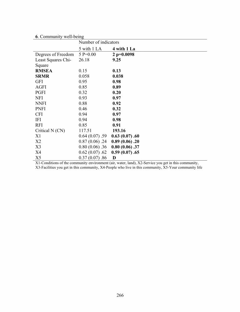
266
6. Community well-being Number of indicators 5 with 1 LA 4 with 1 La Degrees of Freedom 5 P=0.00 2 p=0.0098 Least Squares Chi-Square
26.18 9.25
RMSEA 0.15 0.13 SRMR 0.058 0.038 GFI 0.95 0.98 AGFI 0.85 0.89 PGFI 0.32 0.20 NFI 0.93 0.97 NNFI 0.88 0.92 PNFI 0.46 0.32 CFI 0.94 0.97 IFI 0.94 0.98 RFI 0.85 0.91 Critical N (CN) 117.51 193.16 X1 0.64 (0.07) .59 0.63 (0.07) .60 X2 0.87 (0.06) .24 0.89 (0.06) .20 X3 0.80 (0.06) .36 0.80 (0.06) .37 X4 0.62 (0.07) .62 0.59 (0.07) .65 X5 0.37 (0.07) .86 D X1-Conditions of the community environment (air, water, land), X2-Service you get in this community, X3-Facilities you get in this community, X4-People who live in this community, X5-Your community life
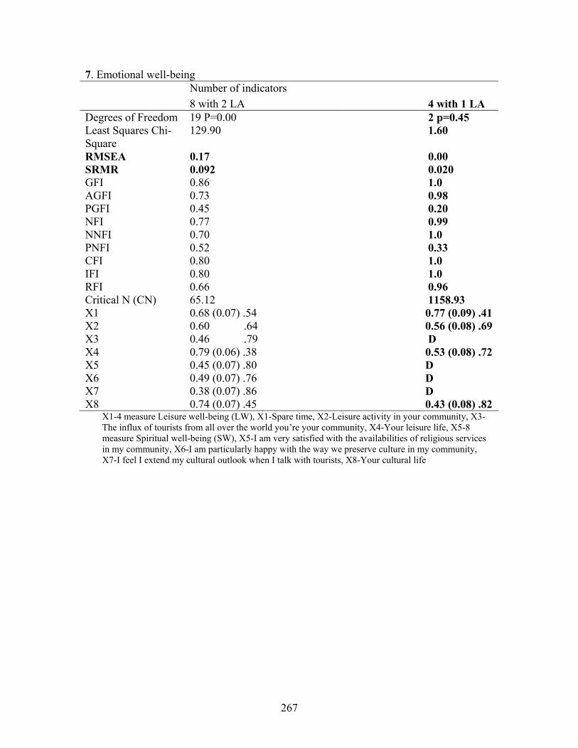
267
7. Emotional well-being Number of indicators 8 with 2 LA 4 with 1 LA Degrees of Freedom 19 P=0.00 2 p=0.45 Least Squares Chi-Square
129.90 1.60
RMSEA 0.17 0.00 SRMR 0.092 0.020 GFI 0.86 1.0 AGFI 0.73 0.98 PGFI 0.45 0.20 NFI 0.77 0.99 NNFI 0.70 1.0 PNFI 0.52 0.33 CFI 0.80 1.0 IFI 0.80 1.0 RFI 0.66 0.96 Critical N (CN) 65.12 1158.93 X1 0.68 (0.07) .54 0.77 (0.09) .41 X2 0.60 .64 0.56 (0.08) .69 X3 0.46 .79 D X4 0.79 (0.06) .38 0.53 (0.08) .72 X5 0.45 (0.07) .80 D X6 0.49 (0.07) .76 D X7 0.38 (0.07) .86 D X8 0.74 (0.07) .45 0.43 (0.08) .82
X1-4 measure Leisure well-being (LW), X1-Spare time, X2-Leisure activity in your community, X3-The influx of tourists from all over the world you’re your community, X4-Your leisure life, X5-8 measure Spiritual well-being (SW), X5-I am very satisfied with the availabilities of religious services in my community, X6-I am particularly happy with the way we preserve culture in my community, X7-I feel I extend my cultural outlook when I talk with tourists, X8-Your cultural life
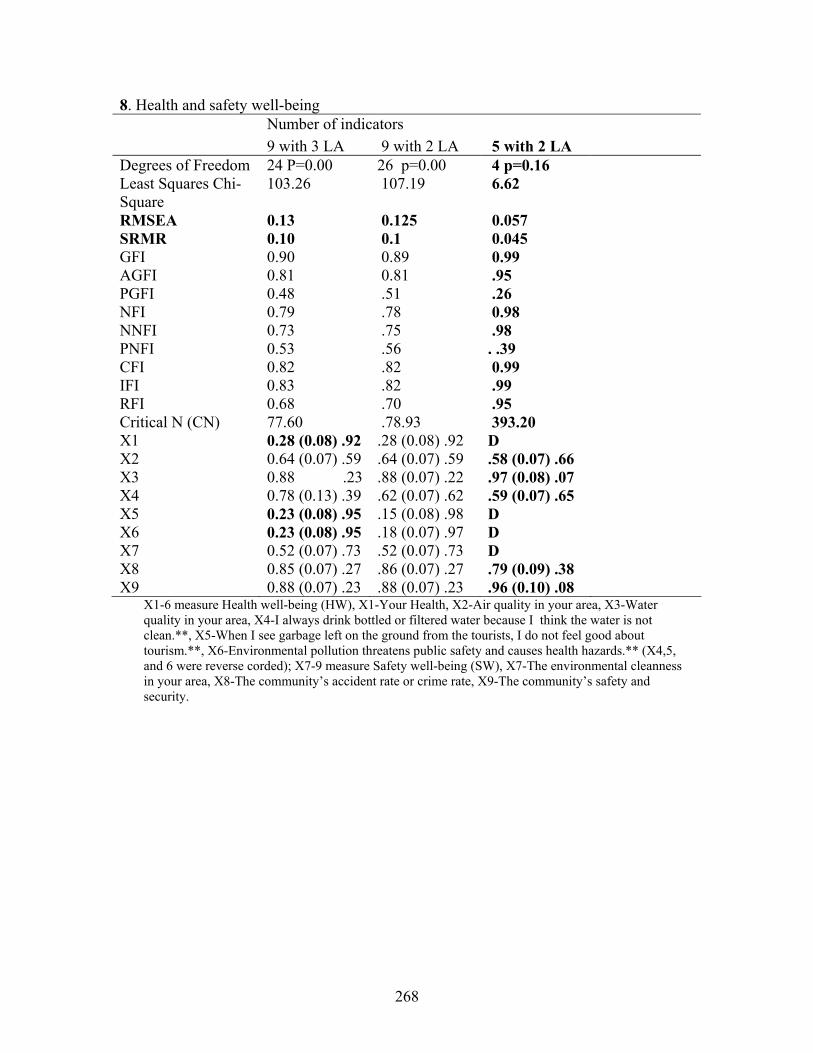
268
8. Health and safety well-being Number of indicators 9 with 3 LA 9 with 2 LA 5 with 2 LA Degrees of Freedom 24 P=0.00 26 p=0.00 4 p=0.16 Least Squares Chi-Square
103.26 107.19 6.62
RMSEA 0.13 0.125 0.057 SRMR 0.10 0.1 0.045 GFI 0.90 0.89 0.99 AGFI 0.81 0.81 .95 PGFI 0.48 .51 .26 NFI 0.79 .78 0.98 NNFI 0.73 .75 .98 PNFI 0.53 .56 . .39 CFI 0.82 .82 0.99 IFI 0.83 .82 .99 RFI 0.68 .70 .95 Critical N (CN) 77.60 .78.93 393.20 X1 0.28 (0.08) .92 .28 (0.08) .92 D X2 0.64 (0.07) .59 .64 (0.07) .59 .58 (0.07) .66 X3 0.88 .23 .88 (0.07) .22 .97 (0.08) .07 X4 0.78 (0.13) .39 .62 (0.07) .62 .59 (0.07) .65 X5 0.23 (0.08) .95 .15 (0.08) .98 D X6 0.23 (0.08) .95 .18 (0.07) .97 D X7 0.52 (0.07) .73 .52 (0.07) .73 D X8 0.85 (0.07) .27 .86 (0.07) .27 .79 (0.09) .38 X9 0.88 (0.07) .23 .88 (0.07) .23 .96 (0.10) .08
X1-6 measure Health well-being (HW), X1-Your Health, X2-Air quality in your area, X3-Water quality in your area, X4-I always drink bottled or filtered water because I think the water is not clean.**, X5-When I see garbage left on the ground from the tourists, I do not feel good about tourism.**, X6-Environmental pollution threatens public safety and causes health hazards.** (X4,5, and 6 were reverse corded); X7-9 measure Safety well-being (SW), X7-The environmental cleanness in your area, X8-The community’s accident rate or crime rate, X9-The community’s safety and security.
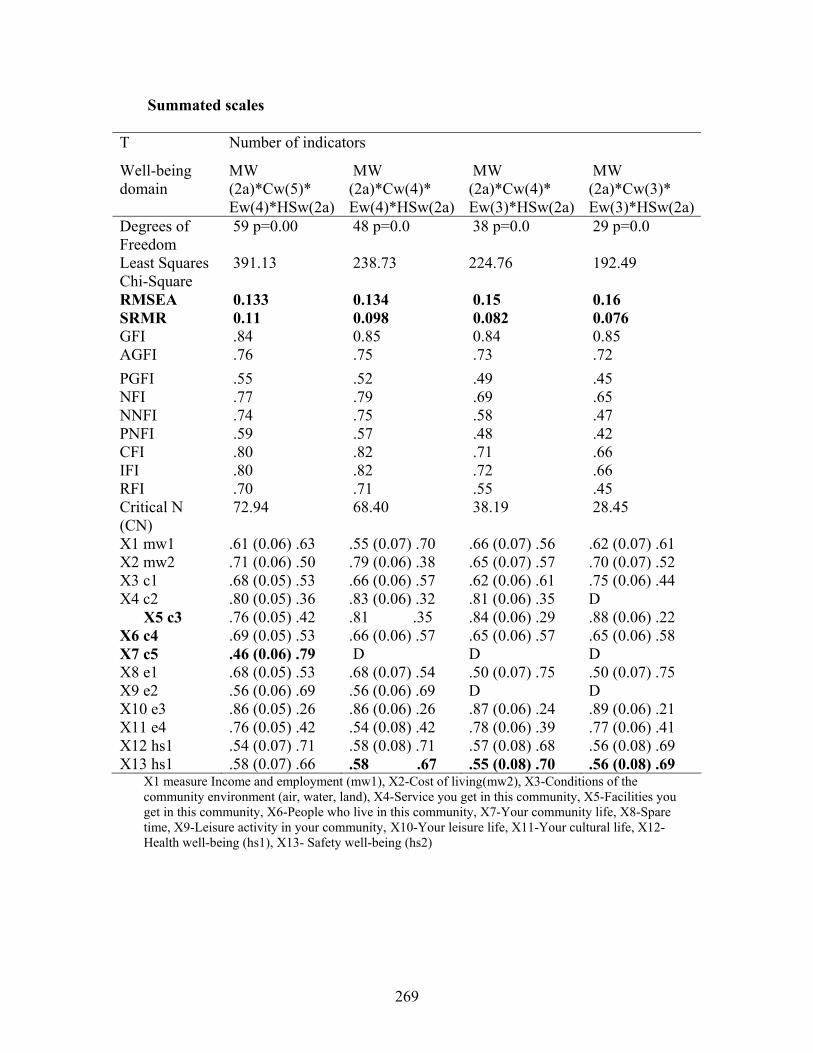
269
Summated scales T Number of indicators
Well-being domain
MW (2a)*Cw(5)* Ew(4)*HSw(2a)
MW (2a)*Cw(4)* Ew(4)*HSw(2a)
MW (2a)*Cw(4)* Ew(3)*HSw(2a)
MW (2a)*Cw(3)* Ew(3)*HSw(2a)
Degrees of Freedom
59 p=0.00 48 p=0.0 38 p=0.0 29 p=0.0
Least Squares Chi-Square
391.13 238.73 224.76 192.49
RMSEA 0.133 0.134 0.15 0.16 SRMR 0.11 0.098 0.082 0.076 GFI .84 0.85 0.84 0.85 AGFI .76 .75 .73 .72 PGFI .55 .52 .49 .45 NFI .77 .79 .69 .65 NNFI .74 .75 .58 .47 PNFI .59 .57 .48 .42 CFI .80 .82 .71 .66 IFI .80 .82 .72 .66 RFI .70 .71 .55 .45 Critical N (CN)
72.94 68.40 38.19 28.45
X1 mw1 .61 (0.06) .63 .55 (0.07) .70 .66 (0.07) .56 .62 (0.07) .61 X2 mw2 .71 (0.06) .50 .79 (0.06) .38 .65 (0.07) .57 .70 (0.07) .52 X3 c1 .68 (0.05) .53 .66 (0.06) .57 .62 (0.06) .61 .75 (0.06) .44 X4 c2 .80 (0.05) .36 .83 (0.06) .32 .81 (0.06) .35 D
X5 c3 .76 (0.05) .42 .81 .35 .84 (0.06) .29 .88 (0.06) .22 X6 c4 .69 (0.05) .53 .66 (0.06) .57 .65 (0.06) .57 .65 (0.06) .58 X7 c5 .46 (0.06) .79 D D D X8 e1 .68 (0.05) .53 .68 (0.07) .54 .50 (0.07) .75 .50 (0.07) .75 X9 e2 .56 (0.06) .69 .56 (0.06) .69 D D X10 e3 .86 (0.05) .26 .86 (0.06) .26 .87 (0.06) .24 .89 (0.06) .21 X11 e4 .76 (0.05) .42 .54 (0.08) .42 .78 (0.06) .39 .77 (0.06) .41 X12 hs1 .54 (0.07) .71 .58 (0.08) .71 .57 (0.08) .68 .56 (0.08) .69 X13 hs1 .58 (0.07) .66 .58 .67 .55 (0.08) .70 .56 (0.08) .69
X1 measure Income and employment (mw1), X2-Cost of living(mw2), X3-Conditions of the community environment (air, water, land), X4-Service you get in this community, X5-Facilities you get in this community, X6-People who live in this community, X7-Your community life, X8-Spare time, X9-Leisure activity in your community, X10-Your leisure life, X11-Your cultural life, X12-Health well-being (hs1), X13- Safety well-being (hs2)
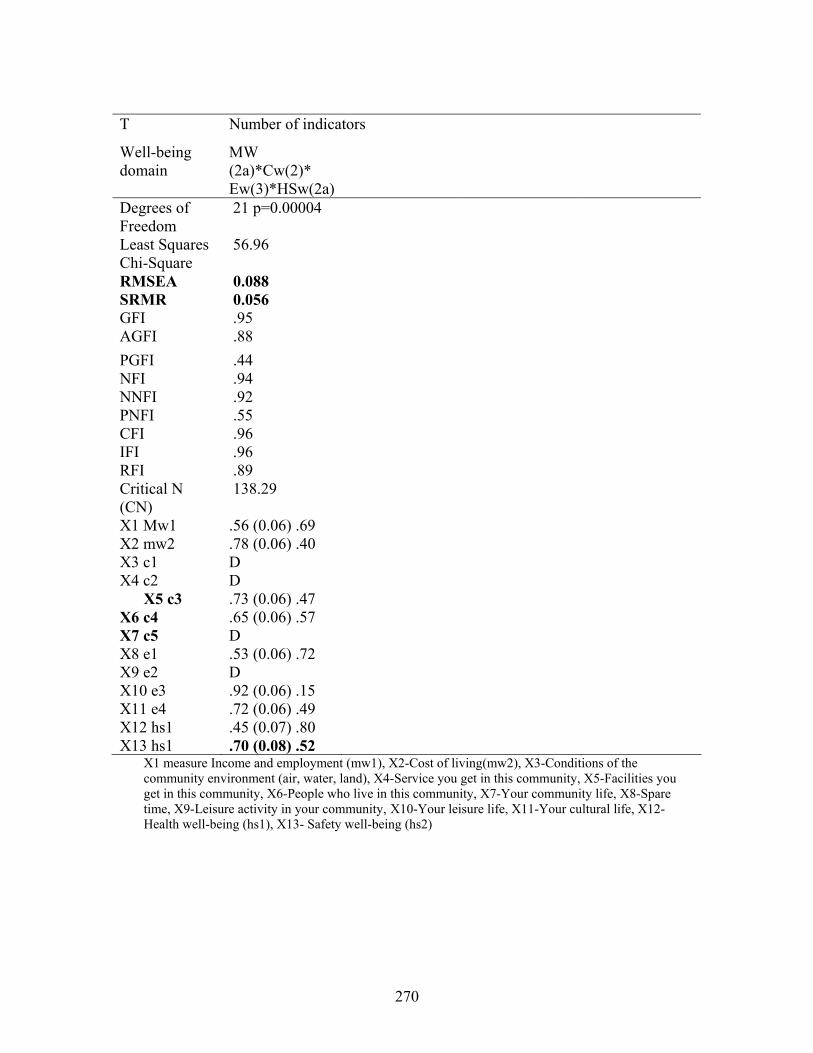
270
T Number of indicators
Well-being domain
MW (2a)*Cw(2)* Ew(3)*HSw(2a)
Degrees of Freedom
21 p=0.00004
Least Squares Chi-Square
56.96
RMSEA 0.088 SRMR 0.056 GFI .95 AGFI .88 PGFI .44 NFI .94 NNFI .92 PNFI .55 CFI .96 IFI .96 RFI .89 Critical N (CN)
138.29
X1 Mw1 .56 (0.06) .69 X2 mw2 .78 (0.06) .40 X3 c1 D X4 c2 D
X5 c3 .73 (0.06) .47 X6 c4 .65 (0.06) .57 X7 c5 D X8 e1 .53 (0.06) .72 X9 e2 D X10 e3 .92 (0.06) .15 X11 e4 .72 (0.06) .49 X12 hs1 .45 (0.07) .80 X13 hs1 .70 (0.08) .52
X1 measure Income and employment (mw1), X2-Cost of living(mw2), X3-Conditions of the community environment (air, water, land), X4-Service you get in this community, X5-Facilities you get in this community, X6-People who live in this community, X7-Your community life, X8-Spare time, X9-Leisure activity in your community, X10-Your leisure life, X11-Your cultural life, X12-Health well-being (hs1), X13- Safety well-being (hs2)

271
Kyungmi Kim
CAMPUS ADDRESS PERMANENT ADDRESS Hunt Club RD. #6200H 103-1002, Sung Won 1 cha Apt. Blacksburg, VA 24060 Joong-gae 1 Dong, Nowon-gu, Phone: (540) 961-7213 Seoul, Korea [email protected] Phone: (822) 938-0246 AREAS OF INTEREST IN RESEARCH AND TEACHING International tourism marketing, Hospitality and tourism marketing, Demand and supply in tourism, Tourist behavior and motivation, Tourism impacts on quality of life, Research methodology in hospitality and tourism, Tourism analysis EDUCATION Doctor of Philosophy in Hospitality and Tourism Management, Virginia Tech, Blacksburg, Virginia, December 2002 Dissertation: The effects of tourism impacts upon Quality of Life of residents in the community. Master of Science in Restaurant Hotel Institutional and Tourism, Purdue University, West Lafayette, Indiana, August 1998 Thesis: Market Segmentation of Japanese Pleasure Travelers based upon Marital Status Bachelor of Science in Economics, Korea University, Seoul, Korea, February 1987 Graduation paper: Tax Structure of Korea PROFESSIONAL EXPERIENCE 2002 Research Assistant, Hospitality and Tourism Management, Virginia Tech, Blacksburg, VA
Conducted research project: developing agricultural tourism, 2001 Instructor, Tourism Analysis (HTM 3454), Hospitality and Tourism Management, Virginia
Tech, Blacksburg, VA 1999-2001 Graduate Teaching Assistant, Hospitality and Tourism Management, Virginia Tech,
Blacksburg, VA
HTM 2454: Introduction to Travel and Tourism Management: A survey of travel and tourism in the United States with focus on terminology, demographics, and financial significance.
HTM 2474: Introduction to Meetings and Convention Management: General overview designed to provide students with information about meetings and convention planning and the industry and define activities of key participants.
272
HTM 3454: Tourism Analysis: Different aspects of tourism, including origin, destination, and impact.
HTM 4984: Attraction Management (Special Study): Provides an understanding of the tourism attractions in the hospitality and tourism industry.
1997-1998 Research Assistant, Hospitality and Tourism Management, Purdue University,
West Lafayette, IN Conducted Research Project: Pittsburgh County Visitor Profile Study
1993 -1995 Marketing Project Officer, Korean Air, Seoul, Korea Planned the tour package program “Joyful Holidays” for Korean Airlines, Promoted
campaign with Korean Red Cross and a major telecommunication company, DACOM 1991-1993 Automation project officer, Korean Air, Seoul, Korea
Participated co-hosting agreements about Computerized Reservation System with SABRE, WORLDSPAN, ABACUS, etc.
1991 Flight Booking Controller, Korean Air, Seoul, Korea Controlled and booked seats for travel agent by using Yield Management System 1987-1990 Computer Programmer, Korean Air, Seoul, Korea
Coded and modified the Computerized Reservation On-line System in Assembler Language
PUBLICATIONS
Papers in Refereed Journals
Kim, K. & Uysal, M. (2003). Perceived socio-economic impacts of festivals and special events: Organizer Perspectives. (In Press) Journal of Hospitality and Leisure Marketing, 10(3/4).
Kim, K, Uysal, M. & Chen, J. (2001). Festival visitor motivation from the organizers’ points of view. Event Management, 7(2), 127-134. Gursoy, D. Kim, K. & Uysal, M. (2002). Developing and testing perceived economic impact scales of festival and event tourism Submitted to Tourism Management.
McGehee, N. & Kim, K. (2002) Farmers’ motivation for agri-tourism business submitted to Journals of Travel Research
Abstracts in Refereed Conference Proceedings
Kim, K. & Uysal M. Effects of tourism impacts upon Quality of Life of residents in the community. Proceedings of International Society for Quality-of-Life Studies (based on the paper presented at the ISQOLS Annual Meeting, Williamsburg, Virginia, November 13-16, 2002).
273
Gursoy, D & Kim, K. (2002). Modeling the cost of travelers’ information search behavior. Proceedings of International CHRIE conference (based on the paper presented at the CHRIE Annual Meeting, Orlando, Florida, August 7-10, 2002). Kim, K., Gursoy, G. (2002). Perceived socio-economic impacts of festivals among organizers. Proceedings of the Seventh Annual Graduate Education and Graduate Student Research Conference in Hospitality and Tourism, p 340-342 (based on the paper presented at the Annual Graduate Education and Graduate Student Research Meeting, Houston, Texas, January 3-5, 2002).
Kim, K. & Uysal, M. (2001). Developing and testing perceived economic impact Scales of festival and event tourism. Proceedings of International CHRIE conference(based on the paper at the CHRIE annual meeting, Toronto, Canada, July 25-28, 2001). Kim, K. (2001). Multivariate methodologies applied to the study of Festival and Event tourism. Proceedings of the Sixth Annual Graduate Education and Graduate Student Research Conference in Hospitality and Tourism, p 249-253 (based on the paper at the Annual Graduate Education and Graduate Student Research Meeting, Atlanta, Georgia, January 4-6, 2001).
PRESENTATIONS AT PROFESSIONAL MEETINGS
Kim, K. & Uysal M. “Effects of tourism impacts upon Quality of Life of residents in the community” was presented at Community Quality of Life Conference, Williamsburg, Virginia, November 13-16, 2002. McGehee, N. & Kim, K. “Agricultural Diversification: Developing Linkages between Agri-tourism Entrepreneurs and Destination Marketing Organizations” was posted at 3rd National Small Farm Conference, Albuquerque, New Mexico, September 17-20, 2002. Gursoy, D & Kim, K. “Modeling the cost of travelers’ information search behavior” was presented at 2002 International CHRIE conference, Orlando, Florida, August 7-10, 2002. Kim, K. & Gursoy, D. “Perceived socio-economic impacts of festivals among organizers” was presented at the Seventh Annual Graduate Education and Graduate Student Research Conference in Hospitality and Tourism, Houston, Texas, January 5-7, 2002. Kim, K. & Uysal, M. “Developing and testing perceived economic impact scales of festival and event tourism” was presented at 2001 International CHRIE conference, Toronto, Canada, July 2001. Kim, K. “As a determinant of tourism demand, destination attractiveness” was presented at the College of Human Resources and Education Faculty Association Meeting and Fourth Annual CHRE Graduate Student Research Day, Blacksburg, Virginia, March 27, 2001. Kim, K. “Multivariate methodologies applied to the study of Festival and Event Tourism” was presented at the Sixth Annual Graduate Education and Graduate Student Research Conference in Hospitality and Tourism, Atlanta, Georgia, January 4-6, 2001.
274
GRANTS AND AWARDS “Graduate Research Development Project” $500 Virginia Tech Graduate Student Association in October, 2002 “Luray Caverns Grant” $2,500 National Tourism Foundation in July 2002 International Marketing Plan Award of the 50th Virginia Conference on World Trade presented by Jim Gilmore, Governor of Virginia, October 14, 1999. Prepare an International Marketing Plan (IMP) for Taylor-Ramsey Inc. to explore potential market in Saudi Arabia. Offered by Virginia Economic Development Partnership (VEDP). Working in a team of four, under the guidance of Dr. Sirgy. Related website: http://www.mba.vt.edu/newsletter/spring00/governor.html PROFESSIONAL SERVICE Women’s President of School of Political and economics, School of Management and School of Law in 1985. Student Member of Oriental Painting Club and “TIME” Magazine Reading Club Membership in Other Organization 1999 – present Student Member of HTM Graduate Association and Minority Student Association 1999 – present Korean Student Association, Virginia Polytechnic Institute and State University 1998 – present Alumni Association in Hospitality and Tourism Management, Purdue University 1987 – present Alumni Association in Economics, Korea University TECHNICAL SKILLS Experience with ASSEMBLY programming language Experience with general computer software Word, Excel, Access, and PowerPoint. Experience with statistical computer software Minitab, SAS, SPSS, MATLAB and LISREL REFERENCES Dr. Muzaffer Uysal ([email protected]) Professor of Hospitality and Tourism Management Virginia Tech, Blacksburg, VA 24061 (540-231-8426) Dr. Ken McCleary ([email protected]) Professor of Hospitality and Tourism Management Virginia Tech, Blacksburg, VA 24061 (540-231-3262) Dr. M. Joseph Sirgy ([email protected]) Professor of Marketing Virginia Tech, Blacksburg, VA 24061 (540-231-5110)