the effects of pan-arctic snow cover and air temperature ... · 5 the effects of pan-arctic snow...
TRANSCRIPT

1
1
Journal of Geophysical Research 2
3
4
The effects of pan-Arctic snow cover and air temperature 5
changes on frozen soil heat content 6
7
8
Xiaogang Shi1 and Dennis P. Lettenmaier
1* 9
10
1Department of Civil and Environmental Engineering, 11
University of Washington, Seattle, Washington, USA 12
13
14
15
16
*Corresponding author: 17
18
Dennis P. Lettenmaier 19
University of Washington 20
Department of Civil and Environmental Engineering, Box 352700 21
Seattle, WA 98195-2700 22
Phone: 206 543 2532 24
Fax: 206 616 6274 25
26
2
Abstract 27
As an indicator of changes in the land surface energy budget, soil heat content (SHC) 28
arguably provides a more complete understanding of high latitude land surface warming than 29
do soil temperatures, which are influenced by surface air temperature (SAT) as well as snow 30
cover extent (SCE). Using the Variable Infiltration Capacity (VIC) land surface model forced 31
with gridded climate observations, we are able to reproduce observed spatial and temporal 32
variations of SCE and SHC over the pan-Arctic land region for the last half-century. On the 33
basis of the SCE trends derived from NOAA satellite observations in 5° latitude bands from 34
April through June for the period 1972-2006, we define a snow covered sensitivity zone 35
(SCSZ), a snow covered non-sensitivity zone (SCNZ), and a non-snow covered zone (NSCZ) 36
for North America and Eurasia. We then explore long-term trends in SHC, SCE, and SAT and 37
their corresponding correlations in NSCZ, SCSZ and SCNZ for both North America and 38
Eurasia. We find that snow cover recession has a significant impact on SHC changes in SCSZ 39
for North America and Eurasia from April through June. SHC changes in SCSZ over North 40
America are dominated by snow cover recession rather than increasing SAT. Over Eurasia, 41
increasing SAT more strongly affects SHC than in North America. Overall, increasing SAT 42
during late spring and early summer has the greatest influence on SHC changes over the pan-43
Arctic, and reduced SCE plays a secondary role, which is only significant in SCSZ. 44

3
1. Introduction 45
Over the pan-Arctic region (for purposes of this paper, defined as the land area draining 46
to the Arctic Ocean), the rise in surface air temperature (SAT) has been almost twice as large 47
as the global average in recent decades [Serreze et al., 2000; Jones and Moberg, 2003; 48
Overland et al., 2004; Hinzman et al., 2005; White et al., 2007; Solomon et al., 2007; 49
Trenberth et al., 2007; Screen and Simmonds, 2010]. Increases in SAT have been accompanied 50
by increasing soil temperatures with deeper active layer thickness across permafrost regions 51
and decreasing frozen soil depths in the seasonally frozen ground regions [Hinzman and Kane, 52
1992; Frauenfeld et al., 2004; Romanovsky et al., 2007]. Given the potential for releases of soil 53
carbon to the atmosphere at warmer temperatures, warming of the land surface at high latitudes 54
has attracted considerable scientific attention [Stieglitz et al., 2003; Heimann and Reichstein, 55
2008]. 56
Observed soil temperatures across the pan-Arctic have been used as an indicator of 57
climate change in past studies [Osterkamp and Romanovsky, 1999; Zhang et al., 2001; Smith 58
et al., 2004; Beltrami et al., 2006; Romanovsky et al., 2002, 2007]. However, in situ soil 59
temperatures are problematic because latent heat effects, which may be significant in regions 60
with frozen soils [Troy, 2010], are neglected. Arguably, the heat content of the soil column is a 61
better indicator of changes in the land surface energy budget because it provides an integrated 62
measure that accounts for changes in temperature, moisture, and latent heat effects. For this 63
reason, it has been used in various studies to document how the land surface responds to 64
atmospheric changes [Levitus et al., 2001, 2005; Beltrami et al., 2002, 2006; Hansen et al., 65
2005; Troy, 2010]. For instance, using the Variable Infiltration Capacity (VIC) land surface 66
4
model [Liang et al., 1994; Cherkauer and Lettenmaier, 1999], Troy et al. [2012] showed that 67
modeled soil temperature profiles and soil heat content (SHC) trends reproduced observed 68
trends at high latitudes. Following these previous studies, we evaluate SHC trends and their 69
causes, with particular attention to the pan-Arctic land region. 70
Because snow is a strong insulator, it limits the efficient communication of heat 71
between the atmosphere and the ground, and thus plays an important role in determining how 72
air temperature signals propagate into the soil column [Gold, 1963; Goodrich, 1982; 73
Osterkamp and Romanovsky, 1996; Stieglitz et al., 2003; Zhang, 2005; Bartlett et al., 2005; 74
Iwata et al., 2008; Lawrence and Slater, 2010]. In general, seasonal snow cover tends to result 75
in relatively higher mean annual ground temperatures, especially at high latitudes where stable 76
snow cover lasts from a few weeks to several months [Zhang, 2005]. 77
In the visible satellite imagery produced by the National Oceanic and Atmospheric 78
Administration (NOAA) [Robinson et al., 1993; Frei and Robinson, 1999], a substantial retreat 79
of snow cover extent (SCE) has been observed during late spring and early summer in recent 80
decades [Groisman et al., 1994; Déry and Brown, 2007; Brown et al., 2010; Shi et al., 2011, 81
2012]. Moreover, these negative SCE trends are well reproduced for both North America and 82
Eurasia by simulations using the VIC model [Shi et al., 2012]. 83
Recent studies have attempted to explain the impact of seasonal snow cover and air 84
temperature on the ground thermal regime over the pan-Arctic by using soil temperature as an 85
index [e.g., Zhang et al., 1997; Zhang and Stamnes, 1998; Romanovsky et al., 2002; Bartlett et 86
al., 2004, 2005; Lawrence and Slater, 2010]. However, the interpretation of relationships 87

5
between seasonal snow cover and air temperature on the ground thermal regime is complicated 88
because surface temperature is affected by multiple variables. An alternative approach is to use 89
SHC as an indicator of changes in the ground thermal regime because it can provide a 90
complete understanding of high latitude land surface warming. 91
In this paper, we explore the effects of snow cover recession and increases in SAT on 92
SHC over the pan-Arctic, with particular emphasis on trends and variability during the late 93
spring and early summer. In section 2, we describe the observations and model-derived data 94
sets on which our analyses are based. In section 3, we explore trends in SHC and examine 95
correlations between SCE, SAT, and SHC and the relative roles of snow cover recession and 96
increasing SAT on SHC changes. 97
2. Data sets 98
2.1. Observed SCE and SAT data 99
Observed monthly values of SCE were extracted from the weekly snow cover and sea 100
ice extent version 3.1 product for the Northern Hemisphere (http://nsidc.org/data/nsidc-101
0046.html), maintained at the National Snow and Ice Data Center (NSIDC). These data span 102
the period October 1966 through June 2007 [Armstrong and Brodzik, 2007]. The data set is 103
based on weekly maps of continental SCE produced by NOAA’s National Environmental 104
Satellite Data and Information Service (NESDIS) [Robinson et al., 1993; Frei and Robinson, 105
1999], which were derived from digitized versions of manual interpretations of Advanced Very 106
High Resolution Radiometer (AVHRR), Geostationary Operational Environmental Satellite 107
(GOES), and other visible band satellite data. We used a version of the data that has been 108

6
regridded to the NSIDC EASE grid with a spatial resolution of 25 km by Armstrong and 109
Brodzik [2007]. Our study is restricted to the period from 1972 on since some charts between 110
1967 and 1971 are missing [Robinson, 2000]. Although ending the time series in 2006 leaves 111
out some exceptionally low Arctic spring SCE values in recent years (e.g., 2008-2010), the 112
non-parametric statistical method we used (section 3.2) is robust to modest changes in the 113
length of the record analyzed. We did not include Greenland in the analyses since its snow 114
cover is mainly perennial in nature. Brown et al. [2010] have compared this SCE record 115
(commonly referred to as the NOAA weekly SCE record) with other available Arctic snow 116
cover data sets. In general, their study and others [e.g., Wiesnet et al., 1987; Robinson et al., 117
1993] have found that the NOAA weekly SCE data are reliable for continental-scale studies of 118
snow cover variability. They have become a widely used tool for deriving trends in climate-119
related studies [Groisman et al., 1994; Déry and Brown, 2007; Flanner et al., 2009; Derksen et 120
al., 2010; Derksen and Brown, 2011; Shi et al., 2011, 2012], notwithstanding uncertainties in 121
some parts of the domain for certain times of the year, such as summertime over northern 122
Canada [Wang et al., 2005]. A more recent update to the data set we used (NOAA snow chart 123
climate data record, CDR) is now available [Brown and Robinson, 2011], but the differences 124
between the new CDR and the data set we used at the pan-Arctic scale are small [Shi et al., 125
2011]. 126
Monthly SAT anomaly data were derived from the Climatic Research Unit [CRU, 127
Brohan et al., 2006] (CRUTEM3 data set from http://www.cru.uea.ac.uk/cru/data/temperature/), 128
which are based on anomalies from the long-term mean temperature for the period 1961-1990 129

7
and are available for each month since 1850. The land-based monthly data are on a regular 0.5° 130
by 0.5° global grid. We regridded these data, including the NOAA SCE observations that were 131
aggregated from the 25-km product, to the 100-km EASE grid using an inverse distance 132
interpolation as implemented in Shi et al. [2012]. 133
2.2. Modeled SHC 134
The version of VIC used for this study is 4.1.2, which includes some updates to the 135
model’s algorithms for cold land processes. For instance, the model includes a snow 136
parameterization that represents snow accumulation and ablation processes using a two-layer 137
energy and mass balance approach [Andreadis et al., 2009], a canopy snow interception 138
algorithm when an overstory is present [Storck et al., 2002], a finite-difference frozen soils 139
algorithm [Cherkauer and Lettenmaier, 1999] with sub-grid frost variability [Cherkauer and 140
Lettenmaier, 2003], and an algorithm for the sublimation and redistribution of blowing snow 141
[Bowling et al., 2004], as well as a lakes and wetlands model [Bowling and Lettenmaier, 2010]. 142
In our implementation of the VIC model, each grid cell is partitioned into five elevation (snow) 143
bands, which can include multiple land cover types (tiles). The snow model is then applied to 144
each tile separately. The current version of the frozen soils algorithm uses a finite difference 145
solution in the algorithm that dates to the work of Cherkauer and Lettenmaier [1999]. To 146
improve spring peak flow predictions, a parameterization of the spatial distribution of soil frost 147
was developed [Cherkauer and Lettenmaier, 2003]. Adam [2007] described some significant 148
modifications to the frozen soils algorithm, including the bottom boundary specification using 149
the observed soil temperature datasets of Zhang et al. [2001], the exponential thermal node 150
distribution, the implicit solver using the Newton-Raphson method, and an excess ground ice 151
8
and ground subsidence algorithm in VIC 4.1.2. In order to model permafrost properly, our 152
implementation used a depth of 15 m with 18 thermal nodes exponentially distributed with 153
depth and a no flux bottom boundary condition [Jennifer Adam, personal communication], 154
which is similar to Troy et al. [2012]. 155
We used the same study domain as documented in Shi et al. [2012], which is defined as 156
all land areas draining into the Arctic Ocean, as well as those regions draining into the Hudson 157
Bay, Hudson Strait, and the Bering Strait, but excluding Greenland (because its snow cover is 158
mainly perennial in nature). The model simulations used calibrated parameters, such as soil 159
depths and infiltration characteristics, from Su et al. [2005]. The off-line VIC runs are at a 160
three-hour time step in full energy balance mode (meaning that the model closes a full surface 161
energy budget by iterating for the effective surface temperature, as contrasted with water 162
balance mode, in which the surface temperature is assumed to equal the surface air temperature) 163
forced with daily precipitation, maximum and minimum temperatures, and wind speed at a 164
spatial resolution (EASE grid) of 100 km. The forcing data were constructed from 1948 165
through 2006 using methods outlined by Adam and Lettenmaier [2008], as described in Shi et 166
al. [2012]. To set the initial conditions including the thermal state in VIC, we initialized the 167
model with a 100-year climatology created by randomly sampling years from the 1948-1969 168
meteorological forcings. Using VIC 4.1.2, we reconstructed SHC from 1970 to 2006 for the 169
pan-Arctic land area. 170
3. Results 171
3.1. Definition of study zones 172
9
The NOAA weekly SCE data (hereafter NOAA-SCE) were analyzed to determine 173
whether or not there are regions with significant changes of NOAA-SCE in North America and 174
Eurasia. On the basis of the SCE trends derived from NOAA-SCE in 5° latitude bands from 175
April through June for the period 1972-2006 as described in Shi et al. [2012], we defined a 176
snow covered sensitivity zone (SCSZ), a snow covered non-sensitivity zone (SCNZ), and a 177
non-snow covered zone (NSCZ) for North America and Eurasia, respectively. 178
Figure 1(a) shows the spatial distribution of long-term monthly means of SCE from 179
NOAA-SCE from April through June for the 35-year period over North American and 180
Eurasian pan-Arctic domains. Figures 1 (b) and (c) illustrate the latitudinal variations of SCE 181
trends and their area fractions over the North American and Eurasian study domains from April 182
through June. The percentage under each bar chart is the trend significance expressed as a 183
confidence level for each 5° of latitude, while the solid line shows the latitudinal patterns in the 184
snow cover area fractions for each month, which in general are at a minimum for the lowest 185
latitude band, and then increase with latitude poleward. 186
Based on the latitudinal changes of NOAA-SCE as shown in Figure 1, we identified 187
different study zones for North America and Eurasia. From April through June, snow mostly 188
covers latitude bands north of 45°N over the pan-Arctic land area, which are denoted as snow 189
covered zones (SCZs) in Figure 1. The rest of the study domains were denoted as non-snow 190
covered zones (NSCZs) (see Figure 1(a) for North America and Eurasia, respectively). Within 191
the SCZs, we selected only those latitudinal bands within which SCE trends were statistically 192
significant for further analyses. For each month, we denoted these bands as snow cover 193
sensitivity zones (SCSZs). For the remaing bands in the SCZs, there is no significant snow 194

10
cover recession, and these bands are defined as snow covered non-sensitivity zones (SCNZs). 195
In Figures 1(b) and 1(c), we use different gray-shaded arrows to highlight the North American 196
and Eurasian SCZs, which include the SCSZs and SCNZs. For example, the SCSZ for May in 197
North America has six latitude bands from 45-50°N to 70-75°N, whereas there is only one 198
band (45-50°N) for the Eurasian SCSZ in April. 199
3.2. Experimental design based on SCE and SAT trends 200
Trend tests were performed on the monthly time series of SCE and SAT area-averaged 201
over the North America and Eurasia study zones. We used the non-parametric Mann-Kendall 202
trend test [Mann, 1945] for trend significance, and the Sen method [Sen, 1968] to estimate 203
their slopes. A 5% significance level (two-tailed test) was used. Tables 1 and 2 summarize the 204
SCE and SAT trends and their significance levels in NSCZ, SCSZ, and SCNZ for both 205
continents from April through June for the entire study period (1972-2006). Table 1 shows that 206
strong statistically significant (p < 0.025) negative trends were detected in SCE for both North 207
American and Eurasian SCSZs, as found in many previous studies. In SCNZ, the decreasing 208
trends in SCE are all non-significant, and the absolute values of trend slopes are much smaller 209
than that in SCSZ. As reported in Table 2, increasing SAT trends were detected for both 210
continents except for North America in May. For June in North America and for May and June 211
in Eurasia, these SAT trends are statistically significant in NSCZ, SCSZ, and SCNZ. In SCNZ, 212
increasing SAT trends are all statistically significant for both continents except for Eurasia in 213
April. 214

11
Based on above long-term trends in SCE and SAT for NSCZ, SCSZ, and SCNZ, it is 215
clear that the impact of increasing SAT on SHC changes can be isolated in NSCZ as there is no 216
presence of snow. In SCSZ, the effects of both SCE and SAT changes on SHC can be 217
compared as indicated in Figure 2. By comparing SCSZ and SCNZ, we can investigate the 218
effect of snow cover recession on SHC changes, as there is snow cover recession in SCSZ 219
whereas none is in SCNZ. Figure 3 shows the area percentages for NSCZ, SCSZ and SCNZ in 220
North America and Eurasia from April through June. In Eurasia, the SCNZ dominates in April 221
as there is no significant snow cover recession for most portions of the study domain. When 222
snow cover retreats, the SCSZ and NSCZ in Eurasia expands significantly in May and June. 223
Over North America, the NOAA-SCE recession occurs earlier than in Eurasia. Especially for 224
May, most regions in North America have snow cover recession. In June, Figure 3 clearly 225
illusrates that SCE is already gone for most portions of Eurasia. 226
3.3. SHC trends 227
Recent studies by Troy et al. [2012] have shown that the VIC model is able to 228
reproduce soil temperature profiles and can be used as a surrogate for (scarce) observations to 229
estimate long-term changes in SHC. To maximize computational efficiency, the spacing of soil 230
thermal nodes in the frozen soils framework in VIC should reflect the variability in soil 231
temperature [Adam, 2007]. Because the greatest variability in soil temperature occurs near the 232
surface, it is preferable to have tighter node spacings near the surface and wider node spacings 233
near the bottom boundary where temperature variability is reduced. Therefore, we used 234
eighteen soil thermal nodes (STNs) distributed exponentially with depth as indicated in Table 3. 235

12
The SHC for each STN in the soil column was calculated for each model time step 236
(three hours) and then aggregated for each month from April through June. Along the soil 237
profile from the top to the bottom, the first STN was named as STN0 with a depth of 0m 238
indicating it is at the surface, while the deepest one is STN17 with a depth of 15m. The SHC 239
for STN17 represents an averaged thermal value for the soil profile. To simplify the analyses, 240
we used the mean monthly SHC in 1970 as zero because the change in soil heat is relative to 241
the datum chosen as described in Troy [2010]. All monthly SHC values are relative to this 242
datum. In addition, monthly SHC anomalies were calculated on the basis of monthly means 243
averaged over each NSCZ, SCSZ and SCNZ of North America and Eurasia by removing the 244
1981-1990 mean. To examine long-term trends in the time series of monthly SHC anomalies, 245
the Mann-Kendall trend test (significance level p < 0.025, two-sided test) and the Sen method 246
as described above were applied. For each study zone, monotonic trend tests were performed 247
on the monthly SHC anomalies averaged over each study zone for each soil thermal node. 248
Figure 4 shows the trends and significance levels of the VIC-derived SHC for each 249
STN in NSCZ, SCSZ and SCNZ over North America and Eurasia from April through June. 250
Figures 4a and 4b show that there are obvious differences for trends and significance levels 251
between North America and Eurasia. For North America (Figure 4a), the SHC in SCSZ 252
increases significantly from the top thermal nodes to the deeper ones, whereas in NSCZ and 253
SCNZ, most thermal nodes have increasing trends, which are not statistically significant. Over 254
Eurasia, this is quite different. In Figure 4b, almost all the thermal nodes in NSCZ, SCSZ, and 255
SCNZ over Eurasia from April through June show statistically significant increasing trends in 256

13
SHC, indicating that there are different effects of snow cover recession and increasing SAT on 257
SHC changes between Eurasia and North America. 258
3.4. Effects of SCE and SAT changes on SHC 259
In order to identify the relative roles of snow cover recession and increasing SAT on 260
pan-Arctic SHC changes, we examined the correlations among SHC, SCE, and SAT over 261
NSCZ, SCSZ and SCNZ for both North America and Eurasia. The Pearson’s product-moment 262
correlation coefficient was computed separately for each study zone from April through June. 263
Given the 35-year record, correlations are statistically significant at a level of p < 0.025 (two-264
sided) when the absolute value of the sample correlation is greater than 0.34 based on the 265
Student t-test with 33 degrees of freedom. Figure 5 shows correlations between observed SCE 266
and VIC-derived SHC in NSCZ, SCSZ, and SCNZ over North America and Eurasia from April 267
through June. In SCSZ, the correlations between SHC and SCE are all statistically significant 268
over both continents from April through June. Over SCNZ, however, the correlations are much 269
smaller and have no statistical significance. These results imply that the static snow cover 270
insulation in SCNZ has a non-significant impact on SHC changes over the pan-Arctic. 271
Additionally, no correlation exists between SHC and SCE in NSCZ. Furthermore, the implied 272
impact of snow cover changes on SHC is similar for North America and Eurasia. 273
Figure 6 shows correlations between observed SAT and simulated SHC monthly time 274
series in NSCZ, SCSZ, and SCNZ over North America and Eurasia from April through June. 275
Overall, the results indicate that SAT has a significant impact on SHC changes in NSCZ. 276
14
Moreover, SAT has greater influence on SHC over Eurasia than in North America as shown in 277
Figure 6. All the correlations over Eurasia are statistically significant except for SCSZ and 278
SCNZ in April, for which the increasing trends in SAT are not statistically significant. 279
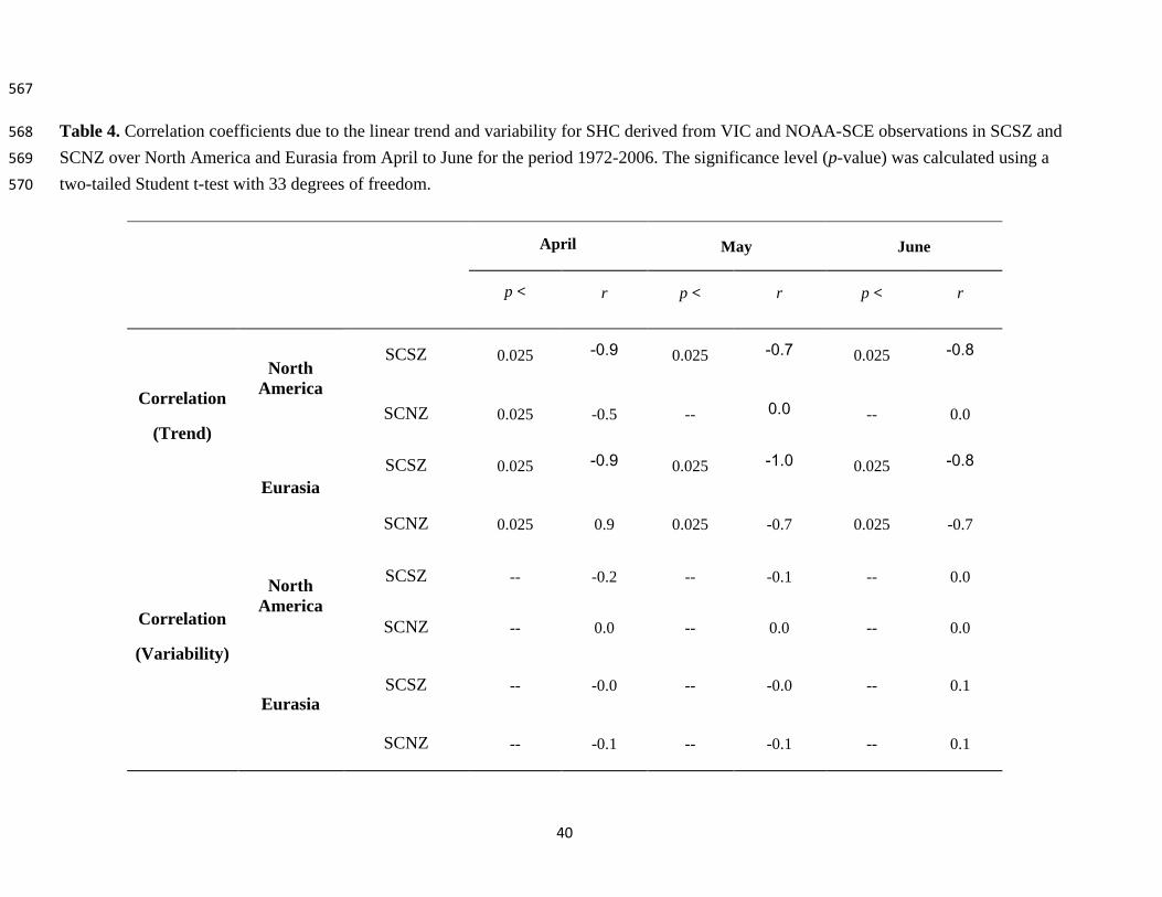
The correlations described in Figures 5 and 6 were calculated on the time series of 280
variables using the Pearson's product-moment method. Both the effects of secular trend and 281
variability are included. We separated these two components and explored the relative roles of 282
the linear trend and the variability (detrended) in the corresponding correlations. Table 4 283
summarizes correlation coefficients due to the linear trend and the variability between SHC 284
derived from VIC and NOAA-SCE observations in SCSZ and SCNZ over North America and 285
Eurasia for the period 1972-2006. The significance level (p-value) was calculated using a two-286
tailed Student t-test with 33 degrees of freedom. Basically, SHC and NOAA-SCE in NSCZ, 287
SCSZ, and SCNZ are highly correlated due to the secular trend, except for May and June in 288
SCNZ over North America, where the NOAA-SCE trends are zero. In contrast, the variability 289
components are small without statistical significance. Obviously, the relationships between 290
SHC and NOAA-SCE time series are mainly dominated by snow cover changes in each study 291
zone over North America and Eurasia. We also applied the same analyses for the VIC-derived 292
SHC and CRU SAT, as reported in Table 5. The linear trends in SAT dominate the correlations 293
between SHC derived from VIC and CRU SAT in NSCZ, SCSZ, and SCNZ over North 294
America and Eurasia for the period 1972-2006. In contrast, the effect of SAT variability is 295
weak and not statistically significant. Therefore, the relationships between SHC and SAT time 296
series as shown in Figure 6 are mainly due to increasing SAT in each study zone over North 297
America and Eurasia. 298

15
As described above, SHC changes are significantly affected by snow cover recession 299
and increasing SAT from April through June over North America and Eurasia for the period 300
1972-2006. But the variablity in NOAA-SCE and SAT has a insignificant effect on SHC. 301
Comparing the correlations in Figures 5 and 6 suggests that: (1) snow cover recession has a 302
significant impact on SHC changes in SCSZ, which is similar for both continents; (2) SHC 303
changes in SCSZ over North America during late spring and early summer are dominated by 304
snow cover recession rather than increasing SAT; (3) over Eurasia, increasing SAT more 305
strongly affects SHC than in North America; and (4) overall, increasing SAT has the greatest 306
influence on SHC for North America and Eurasia, and reduced SCE plays a secondary role, 307
which is only significant in SCSZ. 308
4. Conclusions 309
We defined three study zones (NSCZ, SCSZ, and SCNZ) within the North American 310
and Eurasian portions of the pan-Arctic land area based on observed SCE trends. Using these 311
definitions of zones, we focused on the effects of pan-Arctic snow cover and air temperature 312
changes on SHC by exploring long-term trends in SHC, SCE, and SAT and their 313
corresponding correlations in NSCZ, SCSZ, and SCNZ for North America and Eurasia. We 314
find that North American and Eurasian late spring and early summer (from April through June) 315
SHC has increasing trends for the period 1972-2006. However, there are obvious differences 316
between North America and Eurasia as to the magnitudes of SHC trend slopes and significance 317
levels. For North America, SHC in SCSZ has mostly increased significantly, whereas in NSCZ 318
and SCNZ, most thermal nodes show non-significant increasing trends. For Eurasia, almost all 319
the thermal nodes in NSCZ, SCSZ, and SCNZ have statistically significant increasing trends, 320
16
indicating that there are different effects of snow cover recession and increasing SAT on SHC 321
changes between North America and Eurasia. By analyzing the corresponding correlations, we 322
conclude that snow cover recession has a significant impact on SHC changes in SCSZ for 323
North America and Eurasia from April through June. SHC changes in SCSZ over North 324
America are dominated by snow cover recession rather than increasing SAT. Over Eurasia, 325
increasing SAT more strongly affects SHC than in North America. Overall, increasing SAT 326
during late spring and early summer has the greatest influence on SHC changes over the pan-327
Arctic, and reduced SCE plays a secondary role, which is only significant in SCSZ. 328

17
Acknowledgements 329
This work was supported by NASA grants NNX07AR18G and NNX08AU68G to the 330
University of Washington. The authors thank Dr. Tara Troy from Columbia University, Dr. 331
Jennifer Adam from Washington State University, and Mr. Ted Bohn and Miss Elizabeth Clark 332
from the University of Washington for their assistance and comments. 333
334

18
References 335
Adam, J. C. (2007), Understanding the causes of streamflow changes in the Eurasian Arctic, 336
Ph.D. thesis, 174pp., University of Washington, Seattle, WA. 337
——, and D. P. Lettenmaier (2008), Application of new precipitation and reconstructed 338
streamflow products to streamflow trend attribution in northern Eurasia. J. Clim., 21, 339
1807-1828. 340
Andreadis, K. M., P. Storck, and D. P. Lettenmaier (2009), Modeling snow accumulation and 341
ablation processes in forested environments, Water Resour. Res., 45, W05429, 342
doi:10.1029/2008WR007042. 343
Armstrong, R. L., and M. J. Brodzik (2007), Northern Hemisphere EASE-Grid weekly snow 344
cover and sea ice extent version 3.1, National Snow and Ice Data Center, Boulder, CO, 345
digital media. [Available online at http://nsidc.org/data/nsidc-0046.html.] 346
Bartlett, M. G., D. S. Chapman, and R. N. Harris (2004), Snow and the ground temperature 347
record of climate change, J. Geophys. Res., 109, F04008, doi:10.1029/2004JF000224. 348
Bartlett, M. G., D. S. Chapman, and R. N. Harris (2005), Snow effect on North American 349
ground temperatures, 1950-2002, J. Geophys. Res., 110, F03008, 350
doi:10.1029/2005JF000293. 351
Beltrami, H., J. Smerdon, H. N. Pollack, and S. Huang (2002), Continental heat gain in the 352
global climate system, Geophys. Res. Lett., 29(8), 1167, doi:10.1029/2001GL014310. 353
Beltrami, H., E. Bourlon, L. Kellman, and J. F. Gonza´lez-Rouco (2006), Spatial patterns of 354

19
ground heat gain in the Northern Hemisphere, Geophys. Res. Lett., 33, L06717, 355
doi:10.1029/2006GL025676. 356
Bowling, L. C., J. W. Pomeroy, and D. P. Lettenmaier (2004), Parameterization of blowing-357
snow sublimation in a macroscale hydrology model, J. Hydrometeorol., 5, 745-762. 358
Bowling, L. C., and D. P. Lettenmaier (2010), Modeling the effects of lakes and wetlands on 359
the water balance of arctic environments, J. Hydrometeorol., 11(2), 276-295. 360
Brohan, P., J. Kennedy, I. Harris, S. Tett, and P. Jones (2006), Uncertainty estimates in 361
regional and global observed temperature changes: A new dataset from 1850, J. 362
Geophys. Res., 111, D12106. 363
Brown, R. D., C. Derksen, and L. Wang (2010), A multi-data set analysis of variability and 364
change in Arctic spring snow cover extent, 1967-2008, J. Geophys. Res., 115, D16111. 365
Brown, R. D., and D. A. Robinson (2011), Northern Hemisphere spring snow cover variability 366
and change over 1922–2010 including an assessment of uncertainty, The Cryosphere, 5, 367
219-229. 368
Cherkauer, K. A. and D. P. Lettenmaier (1999) Hydrologic effects of frozen soils in the upper 369
Mississippi River basin, J. Geophys. Res., 104, 19599-19610. 370
—— (2003), Simulation of spatial variability in snow and frozen soil, J. Geophys. Res., 108, 371
8858. 372
Déry, S. J., and R. D. Brown (2007), Recent Northern Hemisphere snow cover extent trends 373
and implications for the snow-albedo feedback, Geophys. Res. Lett., 34, L22504, doi: 374

20
10.1029/2007GL031474. 375
Derksen, C., and R. D. Brown (2011), Terrestrial snow (Arctic) in state of the climate in 2010, 376
Bull. Am. Meteorol. Soc., 92, S154-S155. 377
——, and L. Wang (2010), Terrestrial snow (Arctic) in state of the climate in 2009, Bull. Am. 378
Meteorol. Soc., 91, S93-S94. 379
Flanner, M., C. Zender, P. Hess, N. Mahowald, T. Painter, V. Ramanathan, and P. Rasch 380
(2009), Springtime warming and reduced snow cover from carbonaceous particles, 381
Atmos. Chem. Phys., 9, 2481-2497. 382
Frauenfeld, O. W., T. Zhang, R. G. Barry, and D. Gilichinsky (2004), Interdecadal changes in 383
seasonal freeze and thaw depths in Russia, J. Geophys. Res., 109, D05101, 384
doi:10.1029/2003JD004245 385
Frei, A., and D. A. Robinson (1999), Northern Hemisphere snow extent: Regional variability 386
1972-1994, Int. J. Climatol., 19, 1535-1560. 387
Gold, L. W. (1963), Influence of snow cover on the average annual ground temperature at 388
Ottawa, Canada, IAHS Publ., 61, 82-91. 389
Goodrich, L. E. (1982), The influence of snow cover on the ground thermal regime, Canadian 390
Geotechnical J., 24, 160-163. 391
Groisman, P. Y., T. R. Karl, R. W. Knight, and G. L. Stenchikov (1994), Changes of snow 392
cover, temperature, and radiative heat balance over the Northern Hemisphere, J. Clim., 393
7, 1633-1656. 394
Hansen, J., et al. (2005), Earth’s energy imbalance: Confirmation and implications, Science, 395
21
308, 1431-1435. 396
Heimann, M., and M. Reichstein (2008), Terrestrial ecosystem carbon dynamics and climate 397
feedbacks, Nature, 451(7176), 289-292. 398
Hinzman, L. D., and D. L. Kane (1992), Potential response of an Arctic watershed during a 399
period of global warming, J. Geophys. Res., 97, 2811-2820. 400
Hinzman, L. D., and Coauthors (2005), Evidence and implications of recent climate change in 401
northern Alaska and other arctic regions, Clim. Change, 72, 251-298. 402
Iwata, Y., M. Hayashi, and T. Hirota (2008), Effects of snow cover on soil heat flux and 403
freeze-thaw processes, J. Agric. Meteorol., 64, 301-308. 404
Jones, P. D., and A. Moberg (2003), Hemispheric and large-scale surface air temperature 405
variations: An extensive revision and an update to 2001, J. Clim., 16, 206-223. 406
Lawrence, D. M., and A. G. Slater (2010), The contribution of snow condition trends to future 407
ground climate, Clim. Dyn., 34, 969-981, doi:10.1007/s00382-009-0537-4. 408
Levitus, S., J. Antonov, J. Wang, T. L. Delworth, K. Dixon, and A. Broccoli (2001), 409
Anthropogenic warming of the Earth's climate system, Science, 292, 267-270. 410
Levitus, S., J. Antonov, and T. Boyer (2005), Warming of the world ocean, 1955-2003, 411
Geophys. Res. Lett., 32, L02604, doi:10.1029/2004GL021592. 412
Liang, X., D. P. Lettenmaier, E. Wood, and S. Burges (1994), A simple hydrologically based 413
model of land surface water and energy fluxes for general circulation models, J. 414
Geophys. Res., 99, D17, 14415-14428. 415

22
Mann, H. B. (1945), Nonparametric tests against trend, J. Econom. Sci., 245-259. 416
Osterkamp, T. E., and V. E. Romanovsky (1996), Characteristics of changing permafrost 417
temperatures in the Alaskan Arctic, U.S.A., Arct. Alp. Res., 28(3), 167-273. 418
Osterkamp, T. E., and V. E. Romanovsky (1999), Evidence for warming and thawing of 419
discontinuous permafrost in Alaska, Permafr. Periglac. Process., 10(1), 17-37. 420
Overland, J. E., M. C. Spillane, D. B. Percival, M. Y. Wang, and H. O. Mofjeld (2004), 421
Seasonal and regional variation of pan-Arctic surface air temperature over the 422
instrumental record, J. Clim., 17, 3263-3282. 423
Robinson, D. A. (2000), Weekly Northern Hemisphere snow maps: 1966-1999, Preprints, 12th 424
Conf. on Applied Climatology, Asheville, NC, Amer. Meteor. Soc., 12-15. 425
——, K. F. Dewey, and R. R. Heim Jr (1993), Global snow cover monitoring: An update, Bull. 426
Amer. Meteor. Soc., 74, 1689-1696. 427
Romanovsky, V., S. Smith, K. Yoshikawa, and J. Brown (2002), Permafrost temperature 428
records: indicators of climate change, EOS, Transactions of AGU, 83, 589-594. 429
Romanovsky, V. E., T. S. Sazonova, V. T. Balobaev, N. I. Shender, and D. O. Sergueev (2007), 430
Past and recent changes in air and permafrost temperatures in eastern Siberia, Global 431
Planet. Change, 56, 399-413. 432
Screen, J. A., and I. Simmonds (2010), The central role of diminishing sea ice in recent Arctic 433
temperature amplification, Nature, 464,1334-1337. 434
Sen, P. K. (1968), Estimates of the regression coefficient based on Kendall's tau, J. Am. Stat. 435

23
Assoc., 1379-1389. 436
Serreze, M., and Coauthors (2000), Observational evidence of recent change in the northern 437
high-latitude environment, Clim. Change, 46, 159-207. 438
Shi, X., P. Y. Groisman, S. J. Déry, and D. P. Lettenmaier (2011), The role of surface energy 439
fluxes in pan-Arctic snow cover changes, Environ. Res. Lett., 6, 035204. 440
Shi, X., S. J. Déry, P. Y. Groisman, and D. P. Lettenmaier (2012), Relationships between 441
recent pan-Arctic snow cover and hydroclimate trends, J. Clim. (in press). 442
Smith, N. V., S. S. Saatchi, and J. T. Randerson (2004), Trends in high northern latitude soil 443
freeze and thaw cycle from 1988 to 2002, J. Geophys. Res., 109, D12101, 444
doi:10.1029/2003JD004472 445
Solomon, S., D. Qin, M. Manning, M. Marquis, K. Averyt, M. M. B. Tignor, H. L. Miller Jr., 446
and Z. Chen, Eds. (2007), Clim. Change 2007: The Physical Science Basis, Cambridge 447
University Press, 996 pp. 448
Stieglitz, M., S. J. Déry, V. E. Romanovsky, and T. E. Osterkamp (2003), The role of snow 449
cover in the warming of arctic permafrost, Geophys. Res. Lett., 30, 1721, doi: 450
10.1029/2003GL017337. 451
Storck, P., D. P. Lettenmaier, and S. M. Bolton (2002), Measurement of snow interception and 452
canopy effects on snow accumulation and melt in a mountainous maritime climate, 453
Oregon, United States, Water Resour. Res., 38, 1223. 454
Su, F., J. C. Adam, L. C. Bowling, and D. P. Lettenmaier (2005), Streamflow simulations of 455

24
the terrestrial Arctic domain, J. Geophys. Res., 110, 0148-0227. 456
Trenberth, K. E., et al. (2007), Observations: Surface and atmospheric climate change, in 457
Climate Change 2007: The Physical Science Basis, contribution of working group I to 458
the fourth assessment report of the intergovernmental panel on climate change, edited 459
by S. Solomon et al., 235-336, Cambridge Univ. Press, New York. 460
Troy, T. J. (2010), The hydrology of northern Eurasia: uncertainty and change in the terrestrial 461
water and energy budgets, Ph.D. thesis, 164pp., Princeton University, Princeton, NJ. 462
——, J. Sheffield, and E. F. Wood (2012), Accelerating soil heat accumulation across northern 463
Eurasia, J. Clim. (submitted). 464
Wang, L., M. Sharp, R. Brown, C. Derksen, and B. Rivard (2005), Evaluation of spring snow 465
covered area depletion in the Canadian Arctic from NOAA snow charts, Remote Sens. 466
Environ., 95, 453-463. 467
White, D., and Coauthors (2007), The arctic freshwater system: changes and impacts, J. 468
Geophys. Res., 112, G04S54, doi:10.1029/2006JG000353. 469
Wiesnet, D., C. Ropelewski, G. Kukla, and D. Robinson (1987), A discussion of the accuracy 470
of NOAA satellite-derived global seasonal snow cover measurements, Proc. Vancouver 471
Symp.: Large Scale Effects of Seasonal Snow Cover, Vancouver, BC, Canada, IAHS 472
Publ. 166, 291-304. 473
Zhang, T., T. E. Osterkamp, and K. Stamnes (1997), Effects of climate on the active layer and 474
permafrost on the North Slope of Alaska, U.S.A., Permafr. Periglac. Process., 8, 45-67. 475

25
Zhang, T., and K. Stamnes (1998), Impact of climatic factors on the active layer and 476
permafrost at Barrow, Alaska, Permafr. Periglac. Process., 9, 229-246. 477
Zhang, T., R. G. Barry, D. Gilichinsky, S. S. Bykhovets, V. A. Sorokovikov, and J. P. Ye 478
(2001), An amplified signal of climatic change in soil temperatures during the last 479
century at Irkutsk, Russia, Clim. Change, 49, 41-76. 480
Zhang, T. (2005), Influence of the seasonal snow cover on the ground thermal regime: An 481
overview, Rev. Geophys., 43, RG4002, doi:10.1029/2004RG000157.482

26
List of Figures
Figure 1. (a) Spatial distribution of monthly mean snow cover extent (SCE) from NOAA 483
satellite observations (OBS) over North America and Eurasia in the pan-Arctic land region 484
(non-snow covered zone (NSCZ) and snow covered zone (SCZ)) for April (top panel), May 485
(middle panel), and June (bottom panel) for the period 1972-2006. The SCE trends in 5° 486
latitude bands and their area fractions over (b) North American and (c) Eurasian SCZ, 487
including the snow covered sensitivity zone (SCSZ) and snow covered non-sensitivity zones 488
(SCNZ) as indicated by the arrows. The percentage under each bar chart is the trend 489
significance for each 5° (N) of latitude (expressed as a confidence level (CL)). 490
Figure 2. Experimental design for accessing the effects of pan-Arctic snow cover and air 491
temperature changes on soil heat content (SHC) in NSCZ, SCSZ, and SCNZ over North 492
America and Eurasia from April through June for the period 1972-2006. 493
Figure 3. Area comparisons of NSCZ, SCSZ, and SCNZ in North America and Eurasia from 494
April through June for the period 1972-2006. 495
Figure 4. Trend analyses for SHC at the depth of each soil thermal node derived from the
VIC model in NSCZ, SCSZ, and SCNZ over (a) North America and (b) Eurasia from April
through June for the period 1972-2006. The significance level (expressed as a CL) was
calculated using a two-sided Mann-Kendall trend test. Trend slope (TS) units are mJm-2
year-1
.
Figure 5. Correlations between NOAA-SCE and simulated SHC in NSCZ, SCSZ, and SCNZ 496
over North America and Eurasia from April through June for the period 1972-2006. The 497
correlation is statistically significant at a level of p < 0.025 when its absolute value is greater 498
than 0.34. 499

27
Figure 6. Correlations between observed SAT and simulated SHC in NSCZ, SCSZ and SCNZ 500
over North America and Eurasia from April through June for the period 1972-2006. The 501
correlation is statistically significant at a level of p < 0.025 when its absolute value is greater 502
than 0.34. 503
504

28
505

29
506
507
508
Figure 1. (a) Spatial distribution of monthly mean snow cover extent (SCE) from NOAA satellite observations (OBS) over North America and 509
Eurasia in the pan-Arctic land region (non-snow covered zone (NSCZ) and snow covered zone (SCZ)) for April (top panel), May (middle 510
panel), and June (bottom panel) for the period 1972-2006. The SCE trends in 5° latitude bands and their area fractions over (b) North 511
American and (c) Eurasian SCZ, including the snow covered sensitivity zone (SCSZ) and snow covered non-sensitivity zones (SCNZ) as 512
indicated by the arrows. The percentage under each bar chart is the trend significance for each 5° (N) of latitude (expressed as a confidence 513
level (CL)). 514

30
515
516
517
518
Figure 2. Experimental design for accessing the effects of pan-Arctic snow cover and air temperature changes on frozen soil heat content 519
(SHC) in NSCZ, SCSZ, and SCNZ over North America and Eurasia from April through June for the period 1972-2006. 520
521
522

31
523
524
525
Figure 3. Area comparisons of NSCZ, SCSZ, and SCNZ in North America and Eurasia from April through June for the period 1972-2006. 526
527
528

32
529
530
0.0 0.2 0.4 0.6 0.8 1.0
STN1
STN2
STN3
STN4
STN5
STN6
STN7
STN8
STN9
STN10
STN11
STN12
STN13
STN14
STN15
STN16
STN17
Trend Slope (MJ/m2/year)
So
il T
her
ma
l N
od
e
North America NSCZ April
0.0 0.2 0.4 0.6 0.8 1.0
STN1
STN2
STN3
STN4
STN5
STN6
STN7
STN8
STN9
STN10
STN11
STN12
STN13
STN14
STN15
STN16
STN17
Trend Slope (MJ/m2/year)
So
il T
her
ma
l N
od
e
North America SCSZ April
98%
99%
99%
99%
99%
99%
99%
0.0 0.2 0.4 0.6 0.8 1.0
STN1
STN2
STN3
STN4
STN5
STN6
STN7
STN8
STN9
STN10
STN11
STN12
STN13
STN14
STN15
STN16
STN17
Trend Slope (MJ/m2/year)
So
il T
her
ma
l N
od
e
North America SCNZ April
99%
95% !
98% !
0.0 0.2 0.4 0.6 0.8 1.0
STN1
STN2
STN3
STN4
STN5
STN6
STN7
STN8
STN9
STN10
STN11
STN12
STN13
STN14
STN15
STN16
STN17
Trend Slope (MJ/m2/year)
So
il T
her
mal
No
de
North America NSCZ May
99%
99%
99%
98%
0.0 0.2 0.4 0.6 0.8 1.0
STN1
STN2
STN3
STN4
STN5
STN6
STN7
STN8
STN9
STN10
STN11
STN12
STN13
STN14
STN15
STN16
STN17
Trend Slope (MJ/m2/year)
So
il T
her
mal
No
de
North America SCSZ May
98%
99%
99%
99%
99%
99%
99%
99% !
99% !
99% !
99% !
99% !
98% !
98% !
95% !
95% !
98% !
0.0 0.2 0.4 0.6 0.8 1.0
STN1
STN2
STN3
STN4
STN5
STN6
STN7
STN8
STN9
STN10
STN11
STN12
STN13
STN14
STN15
STN16
STN17
Trend Slope (MJ/m2/year)
So
il T
her
mal
Nod
e
North America SCNZ May
0.0 0.2 0.4 0.6 0.8 1.0
STN1
STN2
STN3
STN4
STN5
STN6
STN7
STN8
STN9
STN10
STN11
STN12
STN13
STN14
STN15
STN16
STN17
Trend Slope (MJ/m2/year)
So
il T
her
ma
l N
od
e
North America NSCZ June
98%
99%
99%
99%
99%
98% !
99% !
99% !
95% !
95% !
0.0 0.2 0.4 0.6 0.8 1.0
STN1
STN2
STN3
STN4
STN5
STN6
STN7
STN8
STN9
STN10
STN11
STN12
STN13
STN14
STN15
STN16
STN17
Trend Slope (MJ/m2/year)
So
il T
her
ma
l N
od
e
North America SCSZ June
99%
99%
99%
99%
99%
99%
99%
99% !
99% !
98% !
98% !
98% !
95% !
99% !
99% !
99% !
99% !
0.0 0.2 0.4 0.6 0.8 1.0
STN1
STN2
STN3
STN4
STN5
STN6
STN7
STN8
STN9
STN10
STN11
STN12
STN13
STN14
STN15
STN16
STN17
Trend Slope (MJ/m2/year)
So
il T
her
ma
l N
od
e
North America SCNZ June
(a)
531
532
533

33
534
(b)
0.0 0.2 0.4 0.6 0.8 1.0
STN1
STN2
STN3
STN4
STN5
STN6
STN7
STN8
STN9
STN10
STN11
STN12
STN13
STN14
STN15
STN16
STN17
Trend Slope (MJ/m2/year)
So
il T
her
ma
l N
od
e
Eurasia NSCZ April
98%
99%
99%
99%
99%
99%
99%
95%
95%
95%
95%
95% !
0.0 0.2 0.4 0.6 0.8 1.0
STN1
STN2
STN3
STN4
STN5
STN6
STN7
STN8
STN9
STN10
STN11
STN12
STN13
STN14
STN15
STN16
STN17
Trend Slope (MJ/m2/year)
So
il T
her
ma
l N
od
e
Eurasia SCSZ April
99%
99%
99%
99%
99%
99%
99%
99%
99%
98%
95% !
90% !
99% !
0.0 0.2 0.4 0.6 0.8 1.0
STN1
STN2
STN3
STN4
STN5
STN6
STN7
STN8
STN9
STN10
STN11
STN12
STN13
STN14
STN15
STN16
STN17
Trend Slope (MJ/m2/year)
So
il T
her
ma
l N
od
e
Eurasia SCNZ April
99%
99%
99%
99%
99%
99%
99%
99%
95%
98%
99%
99%
99%
99%
99% !
0.0 0.2 0.4 0.6 0.8 1.0
STN1
STN2
STN3
STN4
STN5
STN6
STN7
STN8
STN9
STN10
STN11
STN12
STN13
STN14
STN15
STN16
STN17
Trend Slope (MJ/m2/year)
Soil
Th
erm
al
No
de
Eurasia NSCZ May
99%
99%
99%
99%
99%
99%
99%
99% !
99% !
98% !
98% !
98% !
98% !
99% !
99% !
99% !
99% !
0.0 0.2 0.4 0.6 0.8 1.0
STN1
STN2
STN3
STN4
STN5
STN6
STN7
STN8
STN9
STN10
STN11
STN12
STN13
STN14
STN15
STN16
STN17
Trend Slope (MJ/m2/year)
So
il T
her
ma
l N
od
e
Eurasia SCSZ May
99%
99%
99%
99%
99%
99%
99%
99% !
99% !
98% !
98% !
98% !
95% !
99% !
99% !
99% !
99% !
0.0 0.2 0.4 0.6 0.8 1.0
STN1
STN2
STN3
STN4
STN5
STN6
STN7
STN8
STN9
STN10
STN11
STN12
STN13
STN14
STN15
STN16
STN17
Trend Slope (MJ/m2/year)
So
il T
her
ma
l N
od
e
Eurasia SCNZ May
99%
99%
99%
99%
99%
99%
99%
99% !
99% !
99% !
99% !
99% !
99% !
99% !
99% !
99% !
99% !
0.0 0.2 0.4 0.6 0.8 1.0
STN1
STN2
STN3
STN4
STN5
STN6
STN7
STN8
STN9
STN10
STN11
STN12
STN13
STN14
STN15
STN16
STN17
Trend Slope (MJ/m2/year)
So
il T
her
ma
l N
od
e
Eurasia NSCZ June
99%
99%
99%
99%
99%
99%
99%
99% !
99% !
99% !
99% !
99% !
99% !
99% !
99% !
99% !
99% !
0.0 0.2 0.4 0.6 0.8 1.0
STN1
STN2
STN3
STN4
STN5
STN6
STN7
STN8
STN9
STN10
STN11
STN12
STN13
STN14
STN15
STN16
STN17
Trend Slope (MJ/m2/year)
Soil
Th
erm
al
No
de
Eurasia SCSZ June
99%
99%
99%
99%
99%
99%
99%
99% !
99% !
99% !
99% !
99% !
99% !
99% !
99% !
99% !
99% !
0.0 0.2 0.4 0.6 0.8 1.0
STN1
STN2
STN3
STN4
STN5
STN6
STN7
STN8
STN9
STN10
STN11
STN12
STN13
STN14
STN15
STN16
STN17
Trend Slope (MJ/m2/year)
So
il T
her
ma
l N
od
e
Eurasia SCNZ June
99%
99%
99%
99%
99%
99%
99%
98% !
99% !
99% !
99% !
535
Figure 4. Trend analyses for SHC at the depth of each soil thermal node derived from the VIC model in 536
NSCZ, SCSZ, and SCNZ over (a) North America and (b) Eurasia from April through June for the period 537
1972-2006. The significance level (expressed as a CL) was calculated using a two-sided Mann-Kendall 538
trend test. Trend slope (TS) units are mJm-2
year-1
. 539
540

34
541
542
Figure 5. Correlations between observed SCE and simulated SHC in NSCZ, SCSZ, and SCNZ over North America and Eurasia from April 543
through June for the period 1972-2006. The correlation is statistically significant at a level of p < 0.025 when its absolute value is greater than 544
0.34. 545
546

35
547
548
Figure 6. Correlations between observed SAT and simulated SHC in NSCZ, SCSZ and SCNZ over North America and Eurasia from April 549
through June for the period 1972-2006. The correlation is statistically significant at a level of p < 0.025 when its absolute value is greater than 550
0.34. 551
552

36
553
List of Tables
Table 1. Trend analyses for observed snow cover extent (SCE) in the snow covered
sensitivity zone (SCSZ) and the snow covered non-sensitivity zone (SCNZ) over North
America and Eurasia from April through June for the period 1972-2006. The significance
level (p-value) was calculated using a two-sided Mann-Kendall trend test. Trend slope (ts)
units are year-1
.
554
Table 2. Trend analyses for CRU monthly surface air temperature (SAT) in the non-snow
covered zone (NSCZ), SCSZ, and SCNZ over North America and Eurasia from April through
June for the period 1972-2006. The significance level (p-value) was calculated using a two-
sided Mann-Kendall trend test. Ts units are °Cyear-1
.
Table 3. Eighteen soil thermal nodes (STN) and their corresponding depth (m) from the
surface. The first STN has a depth of 0 m indicating it is at the surface.
555
Table 4. Correlation coefficients due to the linear trend and variability for SHC derived from 556
VIC and NOAA-SCE observations in SCSZ and SCNZ over North America and Eurasia from 557
April to June for the period 1972-2006. The significance level (p-value) was calculated using 558
a two-tailed Student t-test with 33 degrees of freedom. 559
Table 5. Correlation coefficients due to the linear trend and variability for SHC derived from
VIC and CRU SAT in NSCZ, SCSZ, and SCNZ over North America and Eurasia from April
to June for the period 1972-2006. The significance level (p-value) was calculated using a two-
tailed Student t-test with 33 degrees of freedom.

37
Table 1. Trend analyses for observed snow cover extent (SCE) in the snow covered sensitivity zone (SCSZ) and the snow covered
non-sensitivity zone (SCNZ) over North America and Eurasia from April through June for the period 1972-2006. The significance
level (p-value) was calculated using a two-sided Mann-Kendall trend test. Trend slope (ts) units are year-1
.
560
North America Eurasia
April May June April May June
p < ts p < ts p < ts p < ts p < ts p < ts
SCE-SCSZ 0.025 -0.0052 0.01 -0.0026 0.01 -0.0029 0.025 -0.0042 0.01 -0.0035 0.005 -0.0034
SCE-SCNZ -- -0.0002 -- -0.0000 -- -0.0000 -- 0.0003 -- -0.0010 -- -0.0006

38
561
Table 2. Trend analyses for CRU monthly surface air temperature (SAT) in the non-snow covered zone (NSCZ), SCSZ, and SCNZ over North
America and Eurasia from April through June for the period 1972-2006. The significance level (p-value) was calculated using a two-sided
Mann-Kendall trend test. Ts units are °Cyear-1
.
562
North America Eurasia
April May June April May June
p < ts p < ts p < ts p < ts p < ts p < ts
SAT-NSCZ -- 0.0345 -- -0.0243 0.005 0.0323 -- 0.0531 0.005 0.0663 0.005 0.0412
SAT-SCSZ -- 0.0400 -- 0.0243 0.005 0.0415 -- 0.0143 0.005 0.0500 0.005 0.0552
SAT-SCNZ 0.005 0.0657 0.005 0.0806 0.01 0.0467 -- 0.0044 0.005 0.0435 0.005 0.0471
563

39
564
Table 3. Eighteen soil thermal nodes (STN) and their corresponding depth (m) from the surface. The first
STN has a depth of 0 m indicating it is at the surface.
Soil Thermal Node Depth (m)
STN0 0.0
STN1 0.2
STN2 0.4
STN3 0.6
STN4 0.9
STN5 1.3
STN6 1.7
STN7 2.1
STN8 2.7
STN9 3.3
STN10 4.1
STN11 5.1
STN12 6.1
STN13 7.3
STN14 8.8
STN15 10.6
STN16 12.6
STN17 15.0
565
566
40
567
Table 4. Correlation coefficients due to the linear trend and variability for SHC derived from VIC and NOAA-SCE observations in SCSZ and 568
SCNZ over North America and Eurasia from April to June for the period 1972-2006. The significance level (p-value) was calculated using a 569
two-tailed Student t-test with 33 degrees of freedom. 570
April May June
p < r p < r p < r
Correlation
(Trend)
North
America
SCSZ 0.025 -0.9 0.025 -0.7 0.025 -0.8
SCNZ 0.025 -0.5 -- 0.0 -- 0.0
Eurasia
SCSZ 0.025 -0.9 0.025 -1.0 0.025 -0.8
SCNZ 0.025 0.9 0.025 -0.7 0.025 -0.7
Correlation
(Variability)
North
America
SCSZ -- -0.2 -- -0.1 -- 0.0
SCNZ -- 0.0 -- 0.0 -- 0.0
Eurasia SCSZ -- -0.0 -- -0.0 -- 0.1
SCNZ -- -0.1 -- -0.1 -- 0.1

41
571
Table 5. Correlation coefficients due to the linear trend and variability for SHC derived from VIC and CRU SAT in NSCZ, SCSZ, and SCNZ
over North America and Eurasia from April to June for the period 1972-2006. The significance level (p-value) was calculated using a two-tailed
Student t-test with 33 degrees of freedom.
April May June
p < r p < r p < r
Correlation
(Trend)
North
America
NSCZ 0.025 0.3 0.025 -0.7 0.025 0.7
SCSZ 0.025 0.9 0.025 0.7 0.025 0.8
SCNZ 0.025 0.5 -- 0.0 -- 0.0
Eurasia
NSCZ 0.025 0.9 0.025 1.0 0.025 1.0
SCSZ 0.025 0.9 0.025 1.0 0.025 0.8
SCNZ 0.025 1.0 0.025 0.7 0.025 0.7
Correlation
(Variability)
North
America
NSCZ -- 0.2 0.025 0.4 -- 0.37
SCSZ -- 0.1 -- -0.2 -- -0.1
SCNZ -- -0.0 -- -0.2 -- -0.2
Eurasia
NSCZ -- 0.2 -- 0.1 -- 0.2
SCSZ -- 0.0 -- 0.2 -- 0.1
SCNZ -- 0.1 -- 0.1 -- 0.1

42
572