the effects of hydro power plants’ governor …
TRANSCRIPT
THE EFFECTS OF
HYDRO POWER PLANTS’ GOVERNOR SETTINGS ON THE
TURKISH POWER SYSTEM FREQUENCY
A THESIS SUBMITTED TO THE GRADUATE SCHOOL OF NATURAL AND APPLIED SCIENCES
OF MIDDLE EAST TECHNICAL UNIVERSITY
BY
MAHMUT ERKUT CEBECİ
IN PARTIAL FULFILLMENT OF THE REQUIREMENTS FOR
THE DEGREE OF MASTER OF SCIENCE IN
ELECTRICAL AND ELECTRONICS ENGINEERING
FEBRUARY 2008
Approval of thesis: “THE EFFECTS OF HYDRO POWER PLANTS’ GOVERNOR SETTINGS
ON THE TURKISH POWER SYSTEM FREQUENCY” submitted by MAHMUT ERKUT CEBECİ in partial fulfillment of the requirements for the degree of Master of Science in Electrical – Electronics Engineering Department, Middle East Technical University by, Prof. Dr. Canan Özgen
Dean, Graduate School of Natural and Applied Sciences Prof. Dr. İsmet Erkmen Head of Department, Electrical and Electronics Engineering Prof. Dr. Arif Ertaş Supervisor, Electrical and Electronics Engineering, METU Examining Committee Members Prof. Dr. Nevzat Özay (*) Electrical and Electronics Engineering, METU Prof. Dr. Arif Ertaş(**) Electrical and Electronics Engineering, METU Prof. Dr. İsmet Erkmen Electrical and Electronics Engineering, METU Assist. Prof. Dr. Ahmet Hava Electrical and Electronics Engineering, METU Ms. Osman Bülent Tör
Tübitak – UZAY
Date: 08.02.2008 (*) Head of examining committee (**) Supervisor

iii
PLAGIARISM
I hereby declare that all information in this document has been obtained and presented in accordance with academic rules and ethical conduct. I also declare that, as required by these rules and conduct, I have fully cited and referenced all material and results that are not original to this work.
Name, Last name: Mahmut Erkut Cebeci
Signature:
iv
ABSTRACT
THE EFFECTS OF
HYDRO POWER PLANTS’ GOVERNOR SETTINGS ON THE
TURKISH POWER SYSTEM FREQUENCY
Cebeci, Mahmut Erkut
MS, Department of Electrical and Electronics Engineering
Supervisor: Prof. Dr. Arif Ertaş
February 2008, 124 Pages
This thesis proposes a method and develops a mathematical model for determining
the effects of hydro power plants’ governor settings on the Turkish power system
frequency.
The Turkish power system suffers from frequency oscillations with 20 – 30
seconds period. Besides various negative effects on power plants and customers,
these frequency oscillations are one of the most important obstacles before the
interconnection of the Turkish power system with the UCTE (Union for the Co-
ordination of Transmission of Electricity) network.
Taking observations of the system operators and statistical studies as an initial
point, the effects of hydro power plants’ governor settings on the Turkish power
system frequency are investigated.

v
In order to perform system wide simulations, initially mathematical models for
two major hydro power plants and their stability margins are determined. Utilizing
this information a representative power system model is developed. After
validation studies, the effects of hydro power plants’ governor settings on the
Turkish power system frequency are investigated. Further computer simulations
are performed to determine possible effects of changing settings and structure of
HPP governors to system frequency stability.
Finally, further factors that may have negative effects on frequency oscillations are
discussed. The results of study are presented throughout the thesis and summarized
in the “Conclusion and Future Work” chapter.
Keywords – frequency stability, speed governor, transient droop reduction.
vi
ÖZ
HİDRO ELEKTRİK SANTRALLERİN HIZ REGÜLATÖR AYARLARININ TÜRKİYE ELEKTRİK SİSTEMİ
FREKANSINA ETKİLERİ
Cebeci, Mahmut Erkut
Yüksek Lisans, Elektrik – Elektronik Mühendisliği Bölümü
Tez Yöneticisi: Prof. Dr. Arif Ertaş
Şubat 2008, 124 Sayfa
Bu tez, hidro elektrik santrallerin hız regülatör ayarlarının Türkiye elektrik sistemi
frekansına etkilerini tespit etmek için, bir metot önerisi ve model uygulaması
içermektedir.
Türkiye elektrik sisteminde periyodu 20 – 30 saniye olan frekans salınımları
mevcuttur. Santraller ve tüketiciler üzerindeki olumsuz etkilerinin yanı sıra, bu
salınımlar Türkiye elektrik sisteminin UCTE (Union for the Co-ordination of
Transmission of Electricity) sistemi ile birleşmesi önündeki en büyük engellerden
biridir.
Sistem operatörlerinin gözlemlerini ve istatistiki çalışmaları bir başlangıç noktası
kabul ederek, hidro elektrik santrallerin hız regülatör ayarlarının Türkiye elektrik
sistemi frekans kararlılığına etkilerini incelenmiştir.
Tüm sistemi kapsayan simülasyon çalışmaları yapabilmek için öncelikle iki önemli
hidro elektrik santralinin matematiksel modelleri ve karalılık aralıkları
belirlenmiştir. Bu bilgiler kullanılarak temsili bir elektrik sistemi modeli
hazırlanmıştır. Modelin doğrulanmasından sonra hidro elektrik santrallerin hız

vii
regülatör ayarlarının Türkiye elektrik sistemi frekansına etkilerini incelenmiştir.
Bunun yanında hidro elektrik santral hız regülâtörlerinde yapılacak ayar
değişiklileri ya da yapısal değişikliklerin sistem frekansına etkilerini belirlemek
için bilgisayar simülasyonları yapılmıştır.
Son olarak frekans salınımları üzerinde olumsuz etkileri olabilecek diğer etkenler
tartışılmıştır. Sonuçlar tez boyunca sunulmuş ve sonuç kısmında özetlenmiştir.
Anahtar kelimeler – frekans kararlılığı, hız regülatörü, geçici hız düşümü.

viii
To My Parents
My Sister
and My Beloved Fiancée

ix
ACKNOWLEDGMENTS
I would like to thank, first of all, to my supervisor, Prof. Dr. Arif Ertaş, for his
guidance, support and trust in me and my studies.
I also would like to thank the members of Hardware Development and Power
Systems Group of Tübitak – UZAY starting with the group coordinator Abdullah
Nadar. Especially I owe my deepest gratitude to Osman Bülent Tör and Ulaş
Karaağaç, who encouraged and advised me throughout the M.S. study. I also thank
to my colleagues Oğuz Yılmaz, Müfit Altın and Mevlüt Akdeniz for their support
and intimate friendship. Finally I would like to thank all members of group for
creating an excellent working and warm friendship environment.
I also would like to thank Osman Bülent Tör for the facilities provided to me by
“National Power Quality Project (105G129)” which is being conducted in Tübitak
– UZAY.
x
TABLE OF CONTENTS PLAGIARISM .............................................................................................. iii
ABSTRACT.................................................................................................. iv
ÖZ.................................................................................................................. vi
ACKNOWLEDGMENTS............................................................................. ix
TABLE OF CONTENTS............................................................................... x
LIST OF TABLES .......................................................................................xii
LIST OF FIGURES.....................................................................................xiii
CHAPTERS
1.INTRODUCTION....................................................................................... 1
2.GENERAL BACKGROUND..................................................................... 7
2.1. Power System Stability ....................................................................... 7
2.2. Classification of Power System Stability ............................................ 9
2.3. Power System Control....................................................................... 12
2.4. Frequency Control Performance of Turkish Power System.............. 22
2.5. Problem Definition............................................................................ 25
2.6. Contribution to the Problem Solution ............................................... 25
3.POWER PLANT MODEL DESCRIPTIONS .......................................... 28
3.1. Introduction ....................................................................................... 28
3.2. Modeling of Hydro Power Plants...................................................... 28
3.3. Modeling of Thermal Power Plants .................................................. 44
3.4. Modeling of Natural Gas Combined Cycle Power Plants................. 46
4.MODELING AND SIMULATION STUDIES ........................................ 49
4.1. Introduction ....................................................................................... 49
4.2. Field Tests on Atatürk Hydro Power Plant ....................................... 50
4.3. Field Tests on Birecik Hydro Power Plant........................................ 58
4.4. Effects of Controller Settings of Hydro Power Plants on System
Frequency ................................................................................................. 68
4.5. Further Factors Affecting System Frequency ................................... 78
xi
5.CONCLUSION AND FUTURE WORK.................................................. 93
REFERENCES............................................................................................. 97
APPENDICES
A. LINEARISED TURBINE/PENSTOCK MODEL............................ 100
B. LOAD FLOW SIMULATIONS OF INITIAL CONDITIONS
PRIOR TO ISLAND TESTS IN ATATÜRK AND BIRECIK
HYDRO POWER PLANTS................................................................... 103
C. SYSTEM CHARACTERISTIC EQUATION FOR ATATÜRK
HYDRO POWER PLANT..................................................................... 106
D. SYSTEM CHARACTERISTIC EQUATION FOR BIRECIK
HYDRO POWER PLANT..................................................................... 108
E. SYSTEM CHARACTERISTIC EQUATION FOR POWER
CONTROL LOOP OF ATATÜRK HYDRO POWER PLANT ........... 110
F. GENERATION AND CONTROLLER INFORMATION OF
SIMULATION CASES.......................................................................... 111
xii
LIST OF TABLES Table 1-1. Priority List of Power Plants and Their Capacities …………………..26
Table F-1. Generation profile of Case-1 .............................................................. 111
Table F-2. Generation profile of Case-1-a ........................................................... 112
Table F-3. Generation profile of Case-1-b ........................................................... 113
Table F-4. Generation profile of Case-1-c ........................................................... 114
Table F-5. Generation profile of Case-1-d ........................................................... 115
Table F-6. Generation profile of Case-1-e ........................................................... 116
Table F-7. Generation profile of Case-1-f............................................................ 117
Table F-8. Generation profile of Case-1-g ........................................................... 118
Table F-9. Generation profile of Case-1-h ........................................................... 119
Table F-10. Generation profile of Case-1-i .......................................................... 120
Table F-11. Generation profile of Case-1-j .......................................................... 121
Table F-12. Generation profile of Case-1-k ......................................................... 122
Table F-13. Generation profile of Case-2 ............................................................ 123
Table F-14. Generation profile of Case-3 ............................................................ 124
xiii
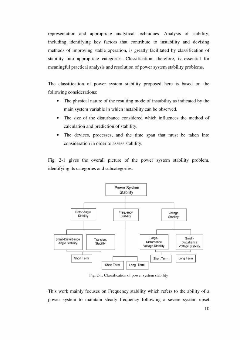
LIST OF FIGURES Fig. 2-1. Classification of power system stability.................................................. 10
Fig. 2-2. Subsystem of a power system and associated controls ........................... 13
Fig. 2-3. Control philosophy .................................................................................. 14
Fig. 2-4. Generator supplying isolated load ........................................................... 15
Fig. 2-5. Schematic of an isochronous governor.................................................... 16
Fig. 2-6. Response of generating unit with isochronous governor......................... 16
Fig. 2-7. Schematic of a governor with speed-droop characteristic....................... 17
Fig. 2-8. Ideal steady-state characteristic of a governor with speed-droop
characteristic........................................................................................................... 18
Fig. 2-9. Load sharing by parallel units with speed-droop characteristics............. 19
Fig. 2-10. Primary control effect after generation loss or load increase ................ 19
Fig. 2-11. Secondary control action ....................................................................... 21
Fig. 2-12. Trumpet curve after an incident............................................................. 23
Fig. 2-13. Frequency recording when major HPP are not in service ..................... 24
Fig. 2-14. Frequency recording when major HPP are in service ........................... 24
Fig. 3-1 Francis Turbine......................................................................................... 29
Fig. 3-2 Typical torque/guide vane characteristic .................................................. 31
Fig. 3-3 Schematic of a HPP .................................................................................. 34
Fig. 3-4 Model of penstock and turbine ................................................................. 36
Fig. 3-5 Turbine power change due to step guide vane opening............................ 37
Fig. 3-6. Speed controller with transient droop compensation .............................. 41
Fig. 3-7a. Open-loop frequency response characteristic with and without transient
droop....................................................................................................................... 41
Fig. 3-7b. Open-loop frequency response characteristic with and without transient
droop....................................................................................................................... 42
Fig. 3-8. Pole positions for different RT and TR settings........................................ 43
Fig. 3-9. Unit response to -200mHz step frequency change for different RT and TR
settings.................................................................................................................... 43
Fig. 3-10. PID speed controller .............................................................................. 44
xiv
Fig. 3-11. Turbine configuration ............................................................................ 44
Fig. 3-12. IEEE standard IEESGO controller and turbine model .......................... 45
Fig. 3-13. A general NGCCPP configuration ........................................................ 47
Fig. 3-14. IEEE standard GAST controller and turbine model.............................. 47
Fig. 4-1. The islanded region during test in Atatürk HPP...................................... 50
Fig. 4-2. The frequency of the islanded region during test in Atatürk HPP........... 51
Fig. 4-3. The speed controller block diagram of Atatürk HPP .............................. 52
Fig. 4-4. The ±200 mHz step response of Unit 8 in Atatürk HPP ......................... 53
Fig. 4-5. The island operation simulations for Atatürk HPP.................................. 54
Fig. 4-6. The block diagram of HPP ...................................................................... 55
Fig. 4-7. The stability boundaries for Atatürk HPP ............................................... 58
Fig. 4-8. The islanded region during test in Birecik HPP ...................................... 59
Fig. 4-9. The island frequency during test in Birecik HPP .................................... 60
Fig. 4-10. The speed controller block diagram of Birecik HPP............................. 60
Fig. 4-11. The island operation simulations for Birecik HPP ................................ 61
Fig. 4-12. The block diagram of HPP with derivative input .................................. 62
Fig. 4-13. The stability boundaries for Birecik HPP.............................................. 64
Fig. 4-14. The second island test in Birecik HPP................................................... 65
Fig. 4-15. The stability limits for Birecik HPP ...................................................... 65
Fig. 4-16. The step response simulation of Birecik HPP ....................................... 66
Fig. 4-17. The stability boundary comparison of Birecik HPP.............................. 67
Fig. 4-18. The measured frequency in different buses after a disturbance ............ 68
Fig. 4-19. The model utilized for system wide studies. ......................................... 70
Fig. 4-20. The measurement and simulation of generation loss in January 2006
(Case-1). ................................................................................................................. 71
Fig. 4-21. The measurement and simulation of generation loss in April 2006
(Case-2). ................................................................................................................. 72
Fig. 4-22. The measurement and simulation of generation loss in March 2006
(Case-3). ................................................................................................................. 73
Fig. 4-23. Comparison of Case-1 with Case-1-a and Case-1-b.............................. 74
Fig. 4-24. Comparison of Case-1 with Case-1-c and Case-1-d.............................. 75
Fig. 4-25. Comparison of Case-1-d with Case-1-e and Case-1-f ........................... 76
Fig. 4-26. Comparison of Case-1-d with Case-1-g and Case-1-h .......................... 77
xv
Fig. 4-27. Comparison of Case-1-d with Case-1-i and Case-1-j ............................ 78
Fig. 4-28. The schematic of power control driving speed control ......................... 79
Fig. 4-29. Change of power output at 50 Hz by changing speed reference (4%
speed droop) ........................................................................................................... 80
Fig. 4-30. The schematic of power control in parallel with speed control............. 80
Fig. 4-31. The schematic of power control without speed control......................... 81
Fig. 4-32. Power controller structure ..................................................................... 82
Fig. 4-33. Effect of frequency bias on power control in operation with speed
control..................................................................................................................... 83
Fig. 4-34. The power controller block diagram of Atatürk HPP ........................... 84
Fig. 4-35. The ±200 mHz step response of Unit 8 in Atatürk HPP ....................... 85
Fig. 4-36. The block diagram of HPP with power control..................................... 85
Fig. 4-37. Stability limit for Atatürk HPP power control settings ......................... 87
Fig. 4-38. Vane opening after a 1% demand increase (Power Control)................. 88
Fig. 4-39. Controller signal deviations after a 1% demand increase (Power
Control) .................................................................................................................. 89
Fig. 4-40. Comparison of Case-1 with Case-1-k.................................................... 90
Fig. 4-41. The power system model including Secondary Control........................ 91
Fig. 4-42. Comparison of Case-1 with Case-1-m................................................... 92
Fig. B-1. Pre-island load flow simulation results for island test in Atatürk HPP 103
Fig. B-2. Pre-island load flow simulation results for island test in Birecik HPP. 105
1
CHAPTERS
C H A P T E R 1
1. INTRODUCTION
Electrical power systems (also referred as grid or network) may be broadly defined
as the group of equipments that generates electrical power by means of various
sources and transfers this power to customers. Although the first complete electric
power system is built as a DC system at the early 1880s, the DC systems are
superseded by AC systems at the beginning of 1900’s. Almost all of the power
systems that are in operation today are AC systems with a variety of two basic
quantities; voltage level and frequency.
The satisfactory operation of a power system is largely dependent on steadiness of
these two quantities. Voltage level and frequency should remain in a narrow
tolerance band for satisfactory operation of customer devices. However, like most
systems, power systems are subject to changes in operating conditions which may
be severe in nature, like faults in various locations or loss of a major generator
and/or load. This change in operating conditions should be responded to
accordingly in order to keep the voltage magnitude and frequency in an acceptable
band and keep the customer supplied with adequate waveform.
In order to keep voltage level and frequency in a tolerance band, controlling
devices are utilized in generating units. Since voltage level throughout the power
system mainly depends on the reactive power demand and flow, controller devices
respond to voltage level changes by modifying the generator terminal voltages
which change the reactive power outputs of the units. The voltage stability is not in
the scope of this study.
2
The second quantity, frequency, depends on the balance between generated and
dissipated power. An unbalance between these two powers results in a change of
kinetic energy stored in rotating parts of generators which changes the rotation
speed and hence changes the frequency of the network. After any disturbance, unit
controllers reestablish the balance between these two powers, and bring frequency
back to the rated value. This overall process is termed as “Load/Frequency
Control”.
The load/frequency control is performed in three steps. The first step is referred as
the “Primary Control (or Regulation)”. The primary control is performed by
controllers termed as “Speed Governor” installed in power plants. The primary
control is used in order to reestablish the power balance utilizing the spinning
reserve of already operating power plants. It has no interest in bringing frequency
back to rated value, but to keep the frequency constant with an acceptable
deviation from its rated value. The second step is the “Secondary Control”, which
brings frequency back to its rated value (50 Hz in Turkey) by changing generating
unit outputs. It utilizes remaining reserve of operating power plants, or takes into
service units when necessary. With the additional reserve from secondary control,
the generating units that have already provided primary reserve are relieved, and
essentially, the system will be ready for the next possible disturbance. Finally
Tertiary control redistributes reserve by committing generator units considering
other factors including the operational costs of plants, environmental concerns, etc.
The load/frequency control philosophy described above is also being applied in the
Turkish power system. However the power system suffers from sustained
frequency oscillations with 20 – 30 seconds period [5]. These oscillations have
negative effects on plants that are contributing to primary control. Since
oscillations are sustained, all generating units are constantly changing their power
generation by changing the position of regulating valves. This continuous
movement of regulating valves not only wears equipment out but also constantly
changes pressure on pipes that carry water or steam going into turbines. The
3
failure chance on these pipes increases due to constant variation and shocks of
pressure. Hence maintenance and repair costs of plants increase drastically.
Further, these oscillations are an obstacle before the connection of the Turkish
power system with the Union for the Co-ordination of Transmission of Electricity
(UCTE). UCTE is the interconnected power system of almost all European
countries, serving for approximately 450 million people. The interconnection, if
realized, will result in improved system security and economy of operation.
System security will improve by emergency assistance of both systems to each
other. Further, the reserve spared for instances in interconnected system will be
less than the sum of reserves spared by individual systems before interconnection.
This reduced system reserve may be distributed by the most economical way.
Moreover, the most economical units may be utilized which reduce the generation
costs for both systems.
Previously a trail operation was performed between Turkish power system and
UCTE. After the interconnection, the frequency of the overall system remained
stable, however the power flow on interconnection lines begun to oscillate with
peak to peak magnitude of approximately 200 MW and period of 20 – 30 seconds
as the frequency oscillations of Turkish power system. This phenomenon can be
explained as follows: Frequency oscillations are due to the continuous change in
power output of generators. The amount of power output change that results in
frequency oscillations in Turkish power system has a negligible effect on
frequency of UCTE system due to the fact that the inertia of UCTE network is
much larger than the inertia of Turkish power system. However the changes in
power output of the generator affect the load flow resulting in sustained power
oscillations on interconnection lines. Hence it was concluded that the
interconnection of two networks is not sustainable before the elimination of
frequency oscillation in Turkish power system.
The interconnection of Turkish power system with UCTE is an on going project
and as stated above one of the major problems to be solved before interconnection
is the frequency oscillation in Turkish power system. During discussions with
4
National Load Dispatch Center (NLDC) representatives on frequency oscillations,
the frequency measurements are investigated for different operating conditions.
Together with previous statistical studies of NLDC, frequency measurements
indicate that the oscillations increase as the Hydro Power Plant (HPP) contribution
to primary frequency control increase. Although this observation by itself is not
enough to state that oscillations are due to HPPs, it gives an initial approach to
studies for determining the possible reasons behind the problem. This is the main
motivation of this thesis study which focuses on the effects of hydro power plants’
governor settings on the Turkish power system frequency.
In Turkish power system the HPPs generate approximately 30 % of overall
generation, however more than 75 % of the spinning reserve is supplied by HPPs
due to the ±2.5 % reserve agreements of combined cycle power plants and
insufficient coal quality or controller structure of thermal power plants. Hence the
primary regulation characteristic of HPPs has an important role on primary
regulation characteristic of Turkish power system. In UCTE network the amount
of HPP generation is around 5% of overall generation. Hence the system
characteristic is based on other types of plants and any possible negative effects of
HPPs governor settings on system frequency that this thesis focus on cannot be
observed in UCTE system.
In the study, in order to observe the effects of HPPs on frequency oscillations, first
a representative power system model is determined. Given the close linkage
between the plant capacity and its effect on frequency regulation, it is not
necessary to model every plant’s controllers in the system for simulation studies.
Hence a priority list which includes the most important power plants based on their
rating is prepared in a way such that, the overall response of these plants in the
priority list represent the overall response of the power system satisfactorily.
There are three different groups of plants in Turkish power system based on the
source of energy; Natural Gas Combined Cycle Power Plants (NGCCPPs),
Thermal Power Plants (TPPs), and HPPs. Their installed capacity ratio is almost
equal (i.e., ≈30%). The NGCCPPs usually consist of three generators; two gas
5
turbines that burn the natural gas, and one steam turbine that run on the steam
generated by high temperature exhaust gases of single or both gas turbines. The
TPPs consist of boilers that burn coal or other fuel to generate high pressure steam
before steam turbine. Finally the HPPs use the kinetic energy of water as a source
for generation. The most important power plants from each group are selected for
the priority list as discussed in the following chapter.
Given that the study focuses on HPPs, the hydro plant unit controller models are
prepared in detail covering the dynamics and friction of penstock and detailed
actual controller models which are determined by site visits and field tests. The
control philosophy is resolved for each HPP in the priority list via manufacturer
documentation1. In addition, controller structure and settings of two major HPPs,
Atatürk and Birecik, are investigated on site by field tests as described in Chapter
4. On the other hand, no field tests are performed on any TPPs2 or NGCCPPs3 to
validate unit controller. The documentations of major TPPs and NGCCPPs
provided by TEİAŞ are utilized to model their unit controllers. After determining
the unit controller models of individual plants in the priority list, the system model
is built by combining them.
MATLAB/SIMULINK [18] and Power System Simulator for Engineering (PSS/E)
[19], are utilized for modeling and simulation studies performed in this thesis. The
controller models developed by MATLAB software are validated by PSS/E
simulations when necessary.
The initial simulation studies are performed to validate the individual plant models
of Atatürk and Birecik HPP. After determining the plant models, the stability
limits of controller settings are determined for both plants. Acquired results are
1) HPPs in priority list: Altınkaya, Atatürk, Berke, Birecik, Hasanuğurlu, Karakaya,
Keban, Oymapınar 2) TPPs in priority list: Ambalı (Fueloil), Çayırhan, Elbistan (A and B), İskenderun,
Kemerköy, Seyitömer, Soma, Yatağan 3) NGCCPP in priority list: Adapazarı, Aliağa, Ambarlı, Bursa, Gebze, Hamitabat,
Temelli, Unimar
6
used to show the effect of controller setting change on stability and response time
of individual units. Further the effects of structural change (addition of derivative
of frequency deviation as an input) on stability limits are determined.
The representative power system model is determined by individual plant models
and validated by comparison of measurements of three different generation loss
events. The chosen events represent three different loading conditions of the power
system. After validating the model, following studies are performed in order to
determine the effects of HPP controllers on power system frequency;
• Increasing and decreasing the contribution of HPP to primary frequency
control
• Changing the “Speed Droop” setting of HPP controllers (“Speed Droop”
term is defined further in the chapters)
• Changing the settings of Proportional Integral (PI) controller
• Changing the structure of controller by addition of an input (derivative of
frequency deviation)
After studying the effects of hydro power plants’ governor settings on the Turkish
power system frequency, further factors that may have negative effects on
damping of frequency oscillations are introduced as future studies. Sample
simulation studies are performed in order to have an idea about possible effects of
these factors.
In conclusion, mathematical models for two major power plants and their stability
margins are determined. Acquired information is utilized for determining a
representative power system model. Using the validated model, the effects of HPP
speed governors on system frequency are studied. Further, possible effects of
changing settings and structure of HPP governors to system frequency are
investigated. Finally, further factors that may have negative effects on frequency
oscillations are discussed. The results of study are presented throughout the thesis
and summarized in the “Conclusion and Future Work” chapter.
7
C H A P T E R 2
2. GENERAL BACKGROUND
2.1. Power System Stability
Power system stability may be broadly defined as the property of a power system
that enables it to remain in a state of operating equilibrium under normal operating
conditions and to regain an acceptable state of operating equilibrium after being
subjected to a physical disturbance, with most system variables bounded so that
practically the entire system remains intact [1].
The definition applies to an interconnected power system as a whole. Often,
however, the stability of a particular generator or group of generators is also of
interest. A remote generator may lose stability (synchronism) without cascading
instability of the main system. Similarly, stability of particular loads or load areas
may be of interest; motors may lose stability (run down and stall) without
cascading instability of the main system.
The power system is a highly nonlinear system that operates in a constantly
changing environment; loads, generator outputs and key operating parameters
change continually. When subjected to a disturbance, the stability of the system
depends on the initial operating conditions as well as the nature of the disturbance.
8
Stability of a power system is thus a property of the system around an equilibrium
set, i.e., the initial operating condition. In an equilibrium set, the various opposing
forces that exist in the system are equal instantaneously (as in the case of
equilibrium points) or over a cycle (as in the case of slow cyclical variations due to
continuous small fluctuations in loads or aperiodic attractors).
Power systems are subjected to a wide range of disturbances, small and large.
Small disturbances in the form of load changes occur continually; the system must
be able to adjust to the changing conditions and operate satisfactorily. It must also
be able to survive numerous disturbances of a severe nature, such as a short circuit
on a transmission line or loss of a large generator. A large disturbance may lead to
structural changes due to the isolation of the faulted elements.
At an equilibrium set, a power system may be stable for a given (large) physical
disturbance, and unstable for another. It is impractical and uneconomical to design
power systems to be stable for every possible disturbance. The design
contingencies are selected on the basis they have a reasonably high probability of
occurrence. Hence, large-disturbance stability always refers to a specified
disturbance scenario. A stable equilibrium set thus has a finite region of attraction;
the larger the region, the more robust the system with respect to large disturbances.
The region of attraction changes with the operating condition of the power system.
The response of the power system to a disturbance may involve much of the
equipment. For instance, a fault on a critical element followed by its isolation by
protective relays will cause variations in power flows, network bus voltages, and
machine rotor speeds; the voltage variations will actuate both generator and
transmission network voltage regulators; the generator speed variations will
actuate prime mover governors; and the voltage and frequency variations will
affect the system loads to varying degrees depending on their individual
characteristics. Further, devices used to protect individual equipment may respond
to variations in system variables and cause tripping of the equipment, thereby
weakening the system and possibly leading to system instability.
9
If following a disturbance the power system is stable, it will reach a new
equilibrium state with the system integrity preserved i.e., with practically all
generators and loads connected through a single contiguous transmission system.
Some generators and loads may be disconnected by the isolation of faulted
elements or intentional tripping to preserve the continuity of operation of bulk of
the system. Interconnected systems, for certain severe disturbances, may also be
intentionally split into two or more “islands” to preserve as much of the generation
and load as possible. The actions of automatic controls and possibly human
operators will eventually restore the system to normal state. On the other hand, if
the system is unstable, it will result in a run-away or run-down situation; for
example, a progressive increase in angular separation of generator rotors, or a
progressive decrease in bus voltages. An unstable system condition could lead to
cascading outages and a shutdown of a major portion of the power system.
Power systems are continually experiencing fluctuations of small magnitudes.
However, for assessing stability when subjected to a specified disturbance, it is
usually valid to assume that the system is initially in a true steady-state operating
condition.
2.2. Classification of Power System Stability
A typical modern power system is a high-order multivariable process whose
dynamic response is influenced by a wide array of devices with different
characteristics and response rates. Stability is a condition of equilibrium between
opposing forces. Depending on the network topology, system operating condition
and the form of disturbance, different sets of opposing forces may experience
sustained imbalance leading to different forms of instability [1].
Power system stability is essentially a single problem; however, the various forms
of instabilities that a power system may undergo cannot be properly understood
and effectively dealt with by treating it as such. Because of high dimensionality
and complexity of stability problems, it helps to make simplifying assumptions to
analyze specific types of problems using an appropriate degree of detail of system
10
representation and appropriate analytical techniques. Analysis of stability,
including identifying key factors that contribute to instability and devising
methods of improving stable operation, is greatly facilitated by classification of
stability into appropriate categories. Classification, therefore, is essential for
meaningful practical analysis and resolution of power system stability problems.
The classification of power system stability proposed here is based on the
following considerations:
• The physical nature of the resulting mode of instability as indicated by the
main system variable in which instability can be observed.
• The size of the disturbance considered which influences the method of
calculation and prediction of stability.
• The devices, processes, and the time span that must be taken into
consideration in order to assess stability.
Fig. 2-1 gives the overall picture of the power system stability problem,
identifying its categories and subcategories.
Fig. 2-1. Classification of power system stability
This work mainly focuses on Frequency stability which refers to the ability of a
power system to maintain steady frequency following a severe system upset
11
resulting in a significant imbalance between generation and load. It depends on the
ability to maintain/restore equilibrium between system generation and load, with
minimum unintentional loss of load. Instability that may result occurs in the form
of sustained frequency swings leading to tripping of generating units and/or loads
[1].
Severe system upsets generally result in large excursions of frequency, power
flows, voltage, and other system variables, thereby invoking the actions of
processes, controls, and protections that are not modeled in conventional transient
stability or voltage stability studies. These processes may be very slow, such as
boiler dynamics, or only triggered for extreme system conditions, such as
volts/Hertz protection tripping generators. In large interconnected power systems,
this type of situation is most commonly associated with conditions following
splitting of systems into islands. Stability in this case is a question of whether or
not each island will reach a state of operating equilibrium with minimal
unintentional loss of load. It is determined by the overall response of the island as
evidenced by its mean frequency, rather than relative motion of machines.
Generally, frequency stability problems are associated with inadequacies in
equipment responses, poor coordination of control and protection equipment, or
insufficient generation reserve. In isolated island systems, frequency stability
could be of concern for any disturbance causing a relatively significant loss of load
or generation.
During frequency excursions, the characteristic times of the processes and devices
that are activated will range from fraction of seconds, corresponding to the
response of devices such as under-frequency load shedding and generator controls
and protections, to several minutes, corresponding to the response of devices such
as prime mover energy supply systems and load voltage regulators. Therefore, as
identified in Fig. 2-1, frequency stability may be a short-term phenomenon or a
long-term phenomenon. An example of short-term frequency instability is the
formation of an under-generated island with insufficient under-frequency load
shedding such that frequency decays rapidly causing blackout of the island within
a few seconds. On the other hand, more complex situations in which frequency
12
instability is caused by steam turbine over-speed controls or boiler/reactor
protection and controls are longer-term phenomena with the time frame of interest
ranging from tens of seconds to several minutes.
2.3. Power System Control
The function of an electric power system is to convert energy from one of the
naturally available forms to the electrical form and to transport it to the points of
consumption. Energy is seldom consumed in electrical form but is rather converted
to other forms such as heat, light and mechanical energy. The advantage of the
electrical form of energy is that it can be transported and controlled with relative
ease and with higher degree of efficiency and reliability. A properly designed and
operated power system should, therefore, meet the following fundamental
requirements:
1. The system must be able to meet the continually changing load demand for
active and reactive power. Unlike other types of energy, electricity cannot be
conveniently stored in sufficient quantities. Therefore, adequate “spinning”
reserve of active and reactive power should be maintained and approximately
controlled at all times.
2. The system should supply energy at minimum cost and with minimum
ecological impact.
3. The “quality” of power supply must meet certain minimum standards with
regard to the following factors:
3.1. Constancy of frequency
3.2. Constancy of voltage
3.3. Level of reliability
Several levels of controls involving a complex array of devices are used to meet
the above requirements. These are depicted in Fig. 2-2 which identifies the various
subsystems of a power system and the associated controls. In this overall structure,
these are controllers operating directly on individual system elements. In a
generating unit these consist of prime mover controls and excitation controls. The
13
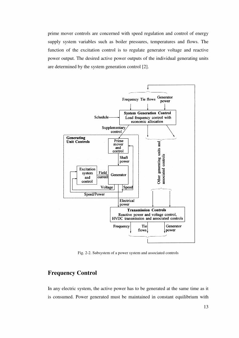
prime mover controls are concerned with speed regulation and control of energy
supply system variables such as boiler pressures, temperatures and flows. The
function of the excitation control is to regulate generator voltage and reactive
power output. The desired active power outputs of the individual generating units
are determined by the system generation control [2].
Fig. 2-2. Subsystem of a power system and associated controls
Frequency Control
In any electric system, the active power has to be generated at the same time as it
is consumed. Power generated must be maintained in constant equilibrium with
14
power consumed / demanded, otherwise a power deviation occurs. Disturbances in
this balance, causing a deviation of the system frequency from its set-point values,
will be offset initially by the kinetic energy of the rotating generating sets and
motors connected. There is only very limited possibility of storing electric energy
as such. It has to be stored as a reservoir (coal, oil, water) for large power systems,
and as chemical energy (battery packs) for small systems. This is insufficient for
controlling the power equilibrium in real-time, so that the production system must
have sufficient flexibility in changing its generation level. It must be able instantly
to handle both changes in demand and outages in generation and transmission,
which preferably should not become noticeable to network users.
The electric frequency in the network is a measure for the rotation speed of the
synchronized generators. By increase in the total demand the system frequency
(speed of generators) will decrease, and by decrease in the demand the system
frequency will increase. Regulating units will then perform automatic primary
control action via load/frequency control (speed governor) and the balance
between demand and generation will be re-established. The frequency deviation is
influenced by both the total inertia in the system, and the speed of prime mover.
Under undisturbed conditions, the system frequency must be maintained within
strict limits in order to ensure the full and rapid deployment of control facilities in
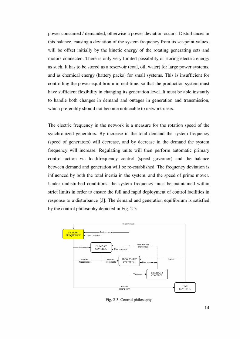
response to a disturbance [3]. The demand and generation equilibrium is satisfied
by the control philosophy depicted in Fig. 2-3.
Fig. 2-3. Control philosophy
15
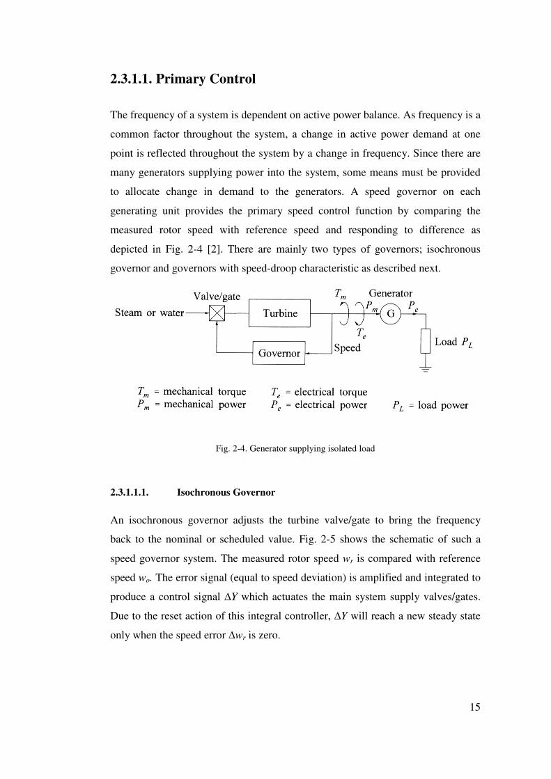
2.3.1.1. Primary Control
The frequency of a system is dependent on active power balance. As frequency is a
common factor throughout the system, a change in active power demand at one
point is reflected throughout the system by a change in frequency. Since there are
many generators supplying power into the system, some means must be provided
to allocate change in demand to the generators. A speed governor on each
generating unit provides the primary speed control function by comparing the
measured rotor speed with reference speed and responding to difference as
depicted in Fig. 2-4 [2]. There are mainly two types of governors; isochronous
governor and governors with speed-droop characteristic as described next.
Fig. 2-4. Generator supplying isolated load
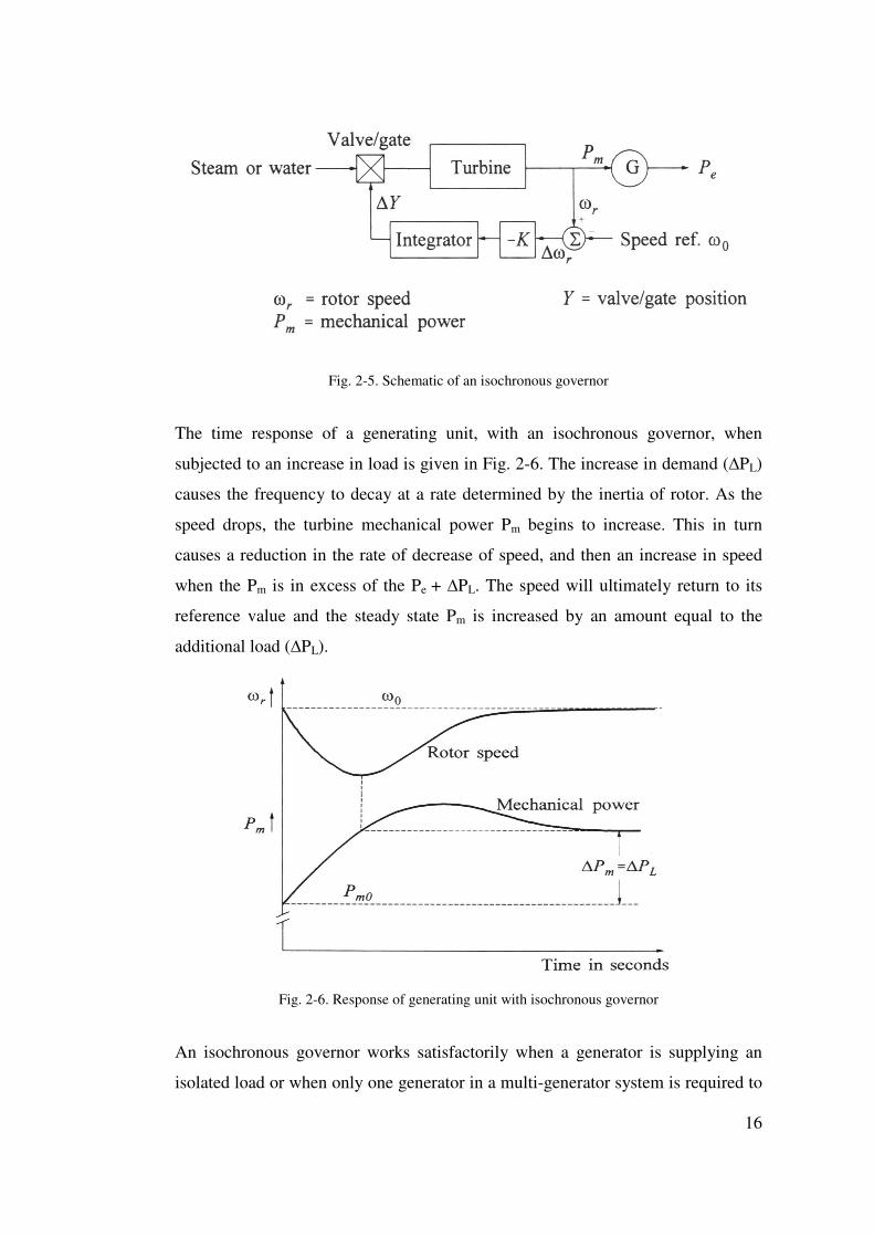
2.3.1.1.1. Isochronous Governor
An isochronous governor adjusts the turbine valve/gate to bring the frequency
back to the nominal or scheduled value. Fig. 2-5 shows the schematic of such a
speed governor system. The measured rotor speed wr is compared with reference
speed wo. The error signal (equal to speed deviation) is amplified and integrated to
produce a control signal ∆Y which actuates the main system supply valves/gates.
Due to the reset action of this integral controller, ∆Y will reach a new steady state
only when the speed error ∆wr is zero.
16
Fig. 2-5. Schematic of an isochronous governor
The time response of a generating unit, with an isochronous governor, when
subjected to an increase in load is given in Fig. 2-6. The increase in demand (∆PL)
causes the frequency to decay at a rate determined by the inertia of rotor. As the
speed drops, the turbine mechanical power Pm begins to increase. This in turn
causes a reduction in the rate of decrease of speed, and then an increase in speed
when the Pm is in excess of the Pe + ∆PL. The speed will ultimately return to its
reference value and the steady state Pm is increased by an amount equal to the
additional load (∆PL).
Fig. 2-6. Response of generating unit with isochronous governor
An isochronous governor works satisfactorily when a generator is supplying an
isolated load or when only one generator in a multi-generator system is required to
17
respond to changes in load. For power load sharing between generators connected
to the system, speed-droop characteristic must be provided as discussed next.
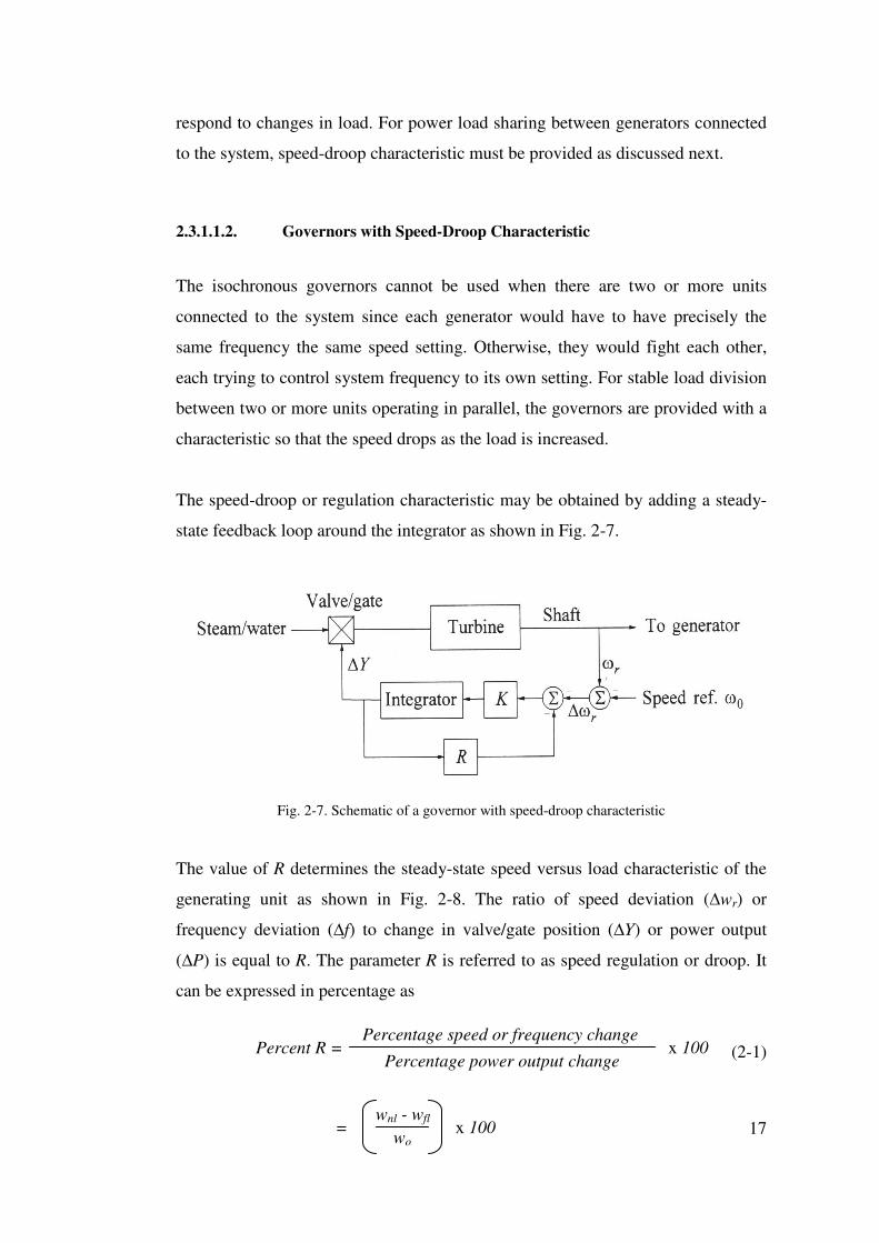
2.3.1.1.2. Governors with Speed-Droop Characteristic
The isochronous governors cannot be used when there are two or more units
connected to the system since each generator would have to have precisely the
same frequency the same speed setting. Otherwise, they would fight each other,
each trying to control system frequency to its own setting. For stable load division
between two or more units operating in parallel, the governors are provided with a
characteristic so that the speed drops as the load is increased.
The speed-droop or regulation characteristic may be obtained by adding a steady-
state feedback loop around the integrator as shown in Fig. 2-7.
Fig. 2-7. Schematic of a governor with speed-droop characteristic
The value of R determines the steady-state speed versus load characteristic of the
generating unit as shown in Fig. 2-8. The ratio of speed deviation (∆wr) or
frequency deviation (∆f) to change in valve/gate position (∆Y) or power output
(∆P) is equal to R. The parameter R is referred to as speed regulation or droop. It
can be expressed in percentage as
(2-1)
Percent R =
Percentage speed or frequency change
Percentage power output change
x 100
=
wnl - wfl
wo
x 100
18
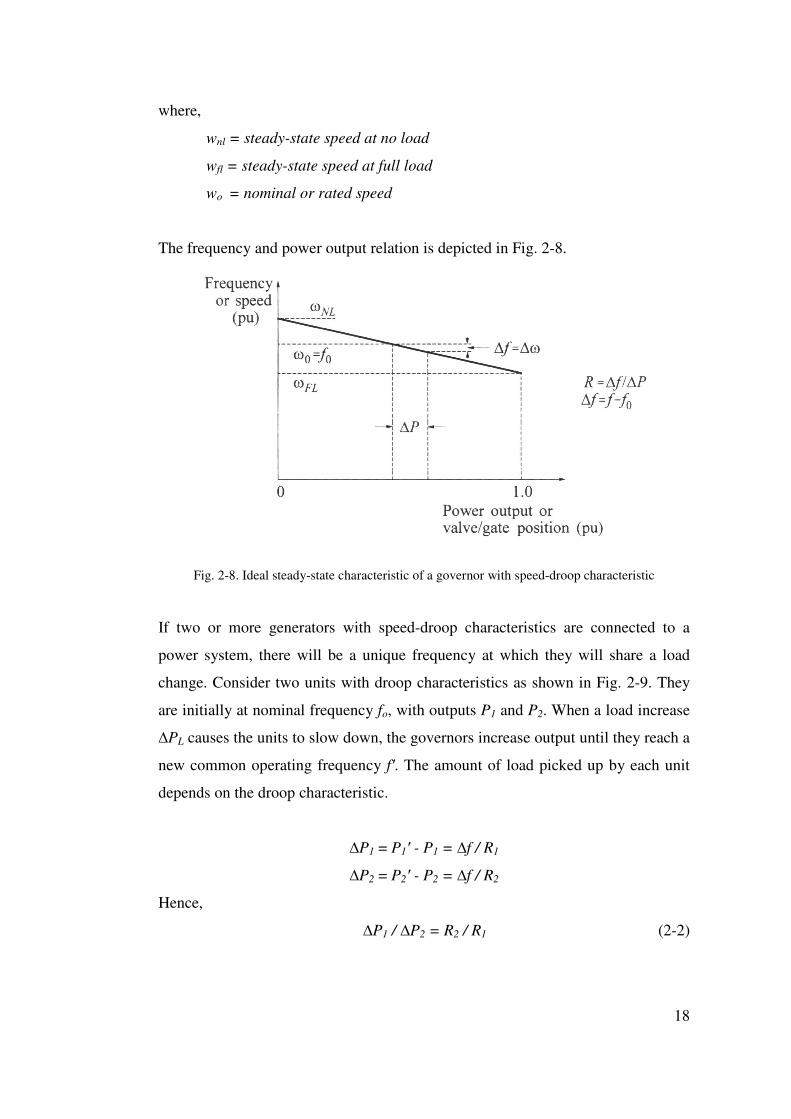
where,
wnl = steady-state speed at no load
wfl = steady-state speed at full load
wo = nominal or rated speed
The frequency and power output relation is depicted in Fig. 2-8.
Fig. 2-8. Ideal steady-state characteristic of a governor with speed-droop characteristic
If two or more generators with speed-droop characteristics are connected to a
power system, there will be a unique frequency at which they will share a load
change. Consider two units with droop characteristics as shown in Fig. 2-9. They
are initially at nominal frequency fo, with outputs P1 and P2. When a load increase
∆PL causes the units to slow down, the governors increase output until they reach a
new common operating frequency f′. The amount of load picked up by each unit
depends on the droop characteristic.
∆P1 = P1′ - P1 = ∆f / R1
∆P2 = P2′ - P2 = ∆f / R2
Hence,
∆P1 / ∆P2 = R2 / R1 (2-2)
19
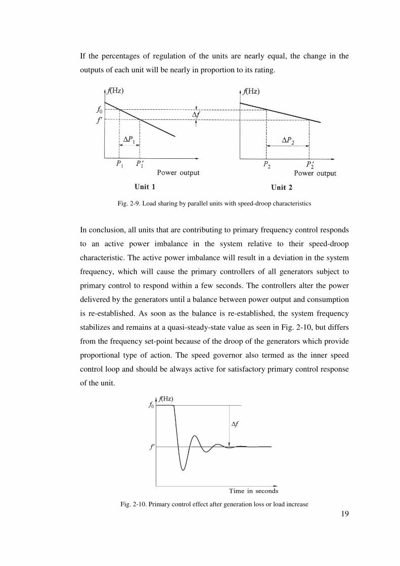
If the percentages of regulation of the units are nearly equal, the change in the
outputs of each unit will be nearly in proportion to its rating.
Fig. 2-9. Load sharing by parallel units with speed-droop characteristics
In conclusion, all units that are contributing to primary frequency control responds
to an active power imbalance in the system relative to their speed-droop
characteristic. The active power imbalance will result in a deviation in the system
frequency, which will cause the primary controllers of all generators subject to
primary control to respond within a few seconds. The controllers alter the power
delivered by the generators until a balance between power output and consumption
is re-established. As soon as the balance is re-established, the system frequency
stabilizes and remains at a quasi-steady-state value as seen in Fig. 2-10, but differs
from the frequency set-point because of the droop of the generators which provide
proportional type of action. The speed governor also termed as the inner speed
control loop and should be always active for satisfactory primary control response
of the unit.
Fig. 2-10. Primary control effect after generation loss or load increase
20
2.3.1.2. Secondary Control
With primary control action, a change in system load will result in a steady-state
frequency deviation, depending on the governor droop characteristic and
frequency sensitivity of the load. All generating units on speed governing will
contribute to the overall change in generation, irrespective of the location of the
load change. Restoration of the system frequency from this quasi-steady-state
value to nominal value requires supplementary control action which adjusts the
load reference set point. Therefore, the basic means of controlling prime-mover
power to match variations in system load in a desired manner is through control of
the load reference set points of selected generating units. As system load is
continually changing, it is necessary to change the output of generators
automatically.
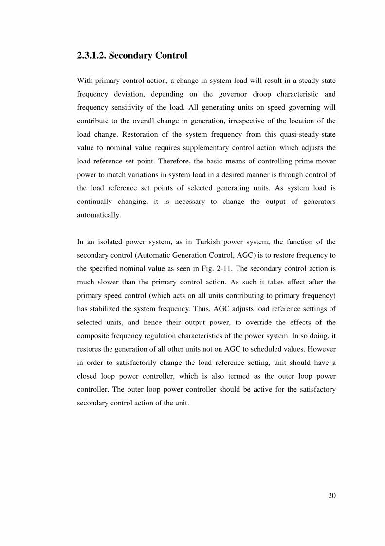
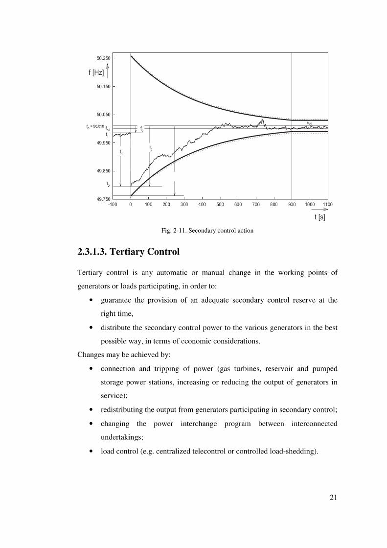
In an isolated power system, as in Turkish power system, the function of the
secondary control (Automatic Generation Control, AGC) is to restore frequency to
the specified nominal value as seen in Fig. 2-11. The secondary control action is
much slower than the primary control action. As such it takes effect after the
primary speed control (which acts on all units contributing to primary frequency)
has stabilized the system frequency. Thus, AGC adjusts load reference settings of
selected units, and hence their output power, to override the effects of the
composite frequency regulation characteristics of the power system. In so doing, it
restores the generation of all other units not on AGC to scheduled values. However
in order to satisfactorily change the load reference setting, unit should have a
closed loop power controller, which is also termed as the outer loop power
controller. The outer loop power controller should be active for the satisfactory
secondary control action of the unit.
21
Fig. 2-11. Secondary control action
2.3.1.3. Tertiary Control Tertiary control is any automatic or manual change in the working points of
generators or loads participating, in order to:
• guarantee the provision of an adequate secondary control reserve at the
right time,
• distribute the secondary control power to the various generators in the best
possible way, in terms of economic considerations.
Changes may be achieved by:
• connection and tripping of power (gas turbines, reservoir and pumped
storage power stations, increasing or reducing the output of generators in
service);
• redistributing the output from generators participating in secondary control;
• changing the power interchange program between interconnected
undertakings;
• load control (e.g. centralized telecontrol or controlled load-shedding).
22
2.4. Frequency Control Performance of Turkish Power System
The frequency control in Turkish power system is performed by primary (through
generating units’ governor action), secondary (by means of central Automatic
Generation Control (AGC) System) and tertiary (manually through instruction
given by National Load Dispatch Center (NLDC)) controls. The participation of
the generating units to the frequency control is described in Turkish Electricity
Market Grid Regulation (Grid Code) as follows;
• All generation facilities with unit capacities of 50 MW and above or total
installed capacity of 100 MW and above except renewable energy
resources shall be obligated to participate in primary frequency control.
• All generation facilities with unit capacities of 50 MW and above or total
installed capacity of 100 MW and above except renewable energy
resources and cogeneration power plants shall also participate in secondary
frequency control within the scope of commercial ancillary services.
• The generation facilities with lower installed capacity may participate in
frequency control only if they submit proposals to Transmission System
Operator (TEİAŞ) and if their proposals are accepted [15].
In line with these regulations, currently all types of power plants are contributing
to frequency control according to their reserve settings determined by the NLDC.
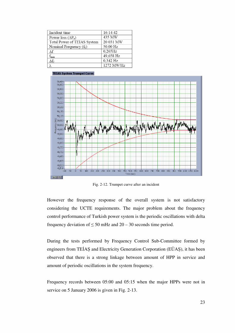
In general, response of the Turkish Power System to the incidences is satisfactory
[5]. As an example, trumpet curve (Fig. 2-12) indicating frequency control
response during the generation loss of 435 MW (Units 1,2 and 3 at Berke HPP) on
25 April 2006 is given below;
23
Fig. 2-12. Trumpet curve after an incident
However the frequency response of the overall system is not satisfactory
considering the UCTE requirements. The major problem about the frequency
control performance of Turkish power system is the periodic oscillations with delta
frequency deviation of ≤ 50 mHz and 20 – 30 seconds time period.
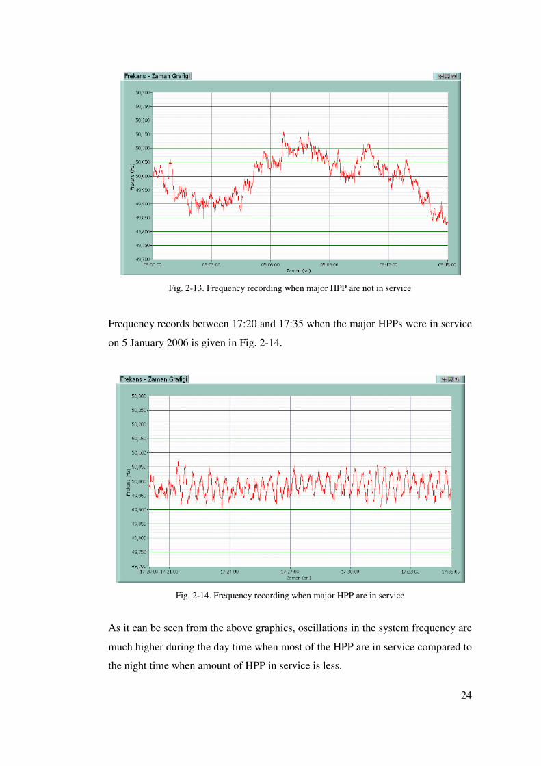
During the tests performed by Frequency Control Sub-Committee formed by
engineers from TEİAŞ and Electricity Generation Corporation (EÜAŞ), it has been
observed that there is a strong linkage between amount of HPP in service and
amount of periodic oscillations in the system frequency.
Frequency records between 05:00 and 05:15 when the major HPPs were not in
service on 5 January 2006 is given in Fig. 2-13.
24
Fig. 2-13. Frequency recording when major HPP are not in service
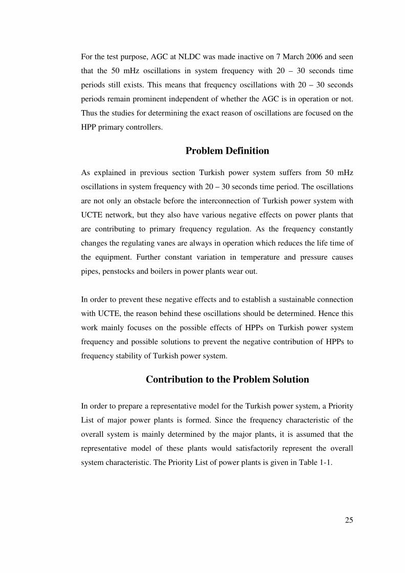
Frequency records between 17:20 and 17:35 when the major HPPs were in service
on 5 January 2006 is given in Fig. 2-14.
Fig. 2-14. Frequency recording when major HPP are in service
As it can be seen from the above graphics, oscillations in the system frequency are
much higher during the day time when most of the HPP are in service compared to
the night time when amount of HPP in service is less.
25
For the test purpose, AGC at NLDC was made inactive on 7 March 2006 and seen
that the 50 mHz oscillations in system frequency with 20 – 30 seconds time
periods still exists. This means that frequency oscillations with 20 – 30 seconds
periods remain prominent independent of whether the AGC is in operation or not.
Thus the studies for determining the exact reason of oscillations are focused on the
HPP primary controllers.
2.5. Problem Definition As explained in previous section Turkish power system suffers from 50 mHz
oscillations in system frequency with 20 – 30 seconds time period. The oscillations
are not only an obstacle before the interconnection of Turkish power system with
UCTE network, but they also have various negative effects on power plants that
are contributing to primary frequency regulation. As the frequency constantly
changes the regulating vanes are always in operation which reduces the life time of
the equipment. Further constant variation in temperature and pressure causes
pipes, penstocks and boilers in power plants wear out.
In order to prevent these negative effects and to establish a sustainable connection
with UCTE, the reason behind these oscillations should be determined. Hence this
work mainly focuses on the possible effects of HPPs on Turkish power system
frequency and possible solutions to prevent the negative contribution of HPPs to
frequency stability of Turkish power system.
2.6. Contribution to the Problem Solution
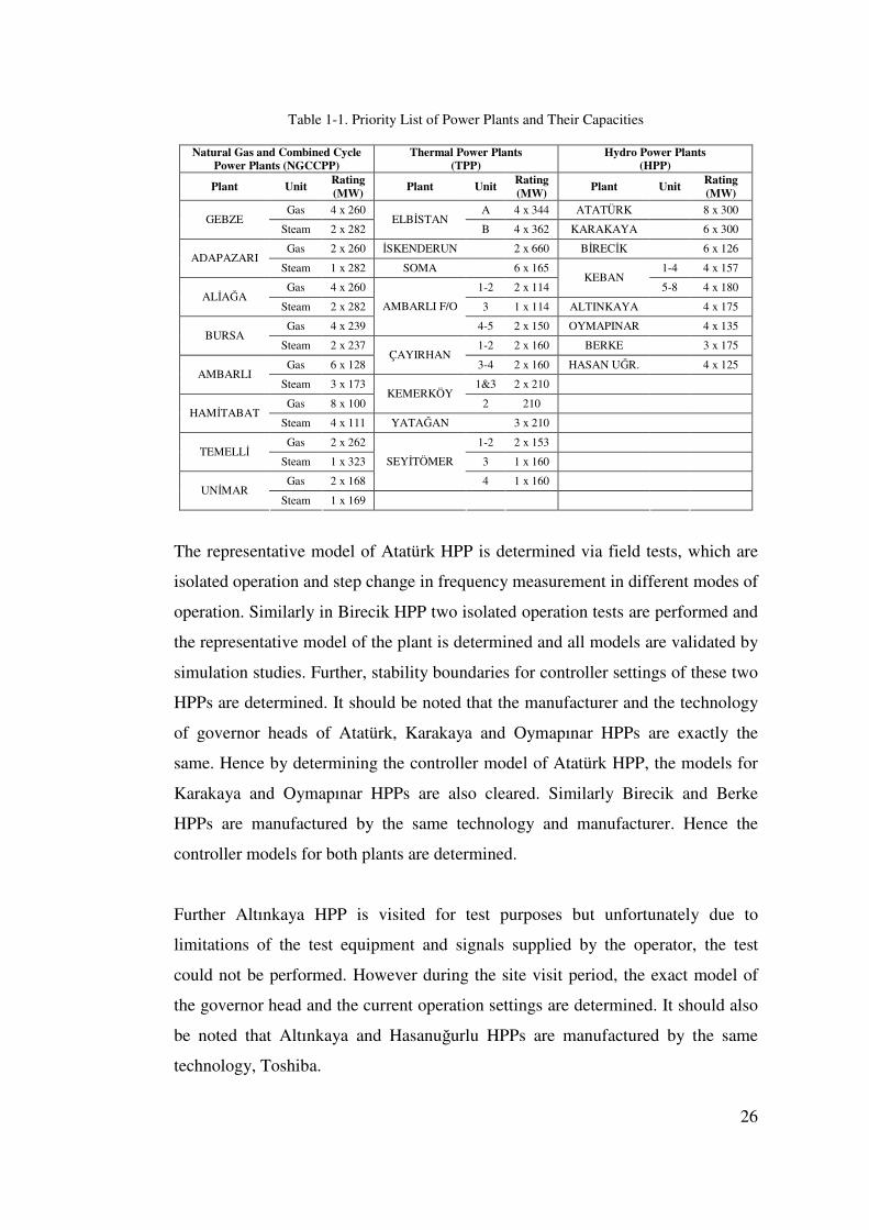
In order to prepare a representative model for the Turkish power system, a Priority
List of major power plants is formed. Since the frequency characteristic of the
overall system is mainly determined by the major plants, it is assumed that the
representative model of these plants would satisfactorily represent the overall
system characteristic. The Priority List of power plants is given in Table 1-1.
26
Table 1-1. Priority List of Power Plants and Their Capacities
Natural Gas and Combined Cycle Power Plants (NGCCPP)
Thermal Power Plants (TPP)
Hydro Power Plants (HPP)
Plant Unit Rating (MW)
Plant Unit Rating (MW)
Plant Unit Rating (MW)
Gas 4 x 260 A 4 x 344 ATATÜRK 8 x 300 GEBZE
Steam 2 x 282 ELBİSTAN
B 4 x 362 KARAKAYA 6 x 300
Gas 2 x 260 İSKENDERUN 2 x 660 BİRECİK 6 x 126 ADAPAZARI
Steam 1 x 282 SOMA 6 x 165 1-4 4 x 157
Gas 4 x 260 1-2 2 x 114 KEBAN
5-8 4 x 180 ALİAĞA
Steam 2 x 282 3 1 x 114 ALTINKAYA 4 x 175
Gas 4 x 239
AMBARLI F/O
4-5 2 x 150 OYMAPINAR 4 x 135 BURSA
Steam 2 x 237 1-2 2 x 160 BERKE 3 x 175
Gas 6 x 128 ÇAYIRHAN
3-4 2 x 160 HASAN UĞR. 4 x 125 AMBARLI
Steam 3 x 173 1&3 2 x 210
Gas 8 x 100 KEMERKÖY
2 210 HAMİTABAT
Steam 4 x 111 YATAĞAN 3 x 210
Gas 2 x 262 1-2 2 x 153 TEMELLİ
Steam 1 x 323 3 1 x 160
Gas 2 x 168
SEYİTÖMER
4 1 x 160 UNİMAR
Steam 1 x 169
The representative model of Atatürk HPP is determined via field tests, which are
isolated operation and step change in frequency measurement in different modes of
operation. Similarly in Birecik HPP two isolated operation tests are performed and
the representative model of the plant is determined and all models are validated by
simulation studies. Further, stability boundaries for controller settings of these two
HPPs are determined. It should be noted that the manufacturer and the technology
of governor heads of Atatürk, Karakaya and Oymapınar HPPs are exactly the
same. Hence by determining the controller model of Atatürk HPP, the models for
Karakaya and Oymapınar HPPs are also cleared. Similarly Birecik and Berke
HPPs are manufactured by the same technology and manufacturer. Hence the
controller models for both plants are determined.
Further Altınkaya HPP is visited for test purposes but unfortunately due to
limitations of the test equipment and signals supplied by the operator, the test
could not be performed. However during the site visit period, the exact model of
the governor head and the current operation settings are determined. It should also
be noted that Altınkaya and Hasanuğurlu HPPs are manufactured by the same
technology, Toshiba.
27
Unfortunately Keban HPP is not visited, but the model of the plant is determined
via discussions with the representatives and experts of VaTech, who is the
manufacturer of the plant. Further the current operational settings are supplied by
the plant operator and the representative model is determined.
For modeling of the NGCCPP and TPP standard IEEE governor models are used
according to the supplied documents and operational settings from plant operators.
Certain assumptions used in the modeling will be described in further chapters.
Finally, representative model for long term frequency stability of Turkish power
system is prepared and validated by previous frequency recordings. After
validating the model, following studies are performed in order to determine the
effects of HPP controllers on power system frequency;
• Increasing and decreasing the contribution of HPP to primary frequency
control
• Changing the “Speed Droop” setting of HPP controllers (“Speed Droop”
term is defined further in the chapters)
• Changing the settings of Proportional Integral (PI) controller
• Changing the structure of controller by addition of an input (derivative of
frequency deviation)
After studying the effects of hydro power plants’ governor settings on the Turkish
power system frequency, other factors that may have negative effects on damping
of frequency oscillations are introduced as future studies, together with sample
simulation studies to have an idea about possible effects of these factors.
28
C H A P T E R 3
3. POWER PLANT MODEL DESCRIPTIONS
3.1. Introduction
This chapter examines the characteristics of hydraulic system, which consists of
turbine and penstock, generator mechanical system and controllers used on HPPs.
The following sections describe the effects of water column characteristics on the
hydraulic turbine performance. The main effect is water inertia in the penstock.
Water column inertia causes changes in the turbine to lag behind changes in the
turbine guide vane opening, which introduces a phase lag into the governor loop
and has a destabilizing effect on the unit. Moreover the dynamic behavior of
generator, converting the mechanical energy into electrical energy is described.
Further the speed control is investigated, including the conflicts between fast
primary control response to frequency deviations and positive effect on power
system frequency stability. Standard IEEE models used in order to model TPPs
and NGCCPPs are also described.
3.2. Modeling of Hydro Power Plants
Hydraulic System Model
3.2.1.1. Turbine Model The oldest form of energy conversion is by the use of waterpower; the turbine
converts the potential energy of the water into the rotational kinetic energy of the
29
turbine. In the traditional hydroelectric scheme the energy is obtained free of cost
as the water comes from a high level reservoir into the turbine in which the water
energy is converted directly to mechanical energy. In the turbine, the tangential
momentum of the water passing through a runner’s blade will be changed in
direction and a tangential force on the runner is produced. The runner therefore
rotates and the energy is transferred from the water to the runner and hence to the
output shaft. The water is discharged with reduced energy. The hydraulic turbine
may be classified into one of two general categories: impulse and reaction [6].
Although there are many applications of impulse turbines around the world none
of the priority list HPPs has an impulse type turbine. Hence the impulse turbine
model is not investigated in this study.
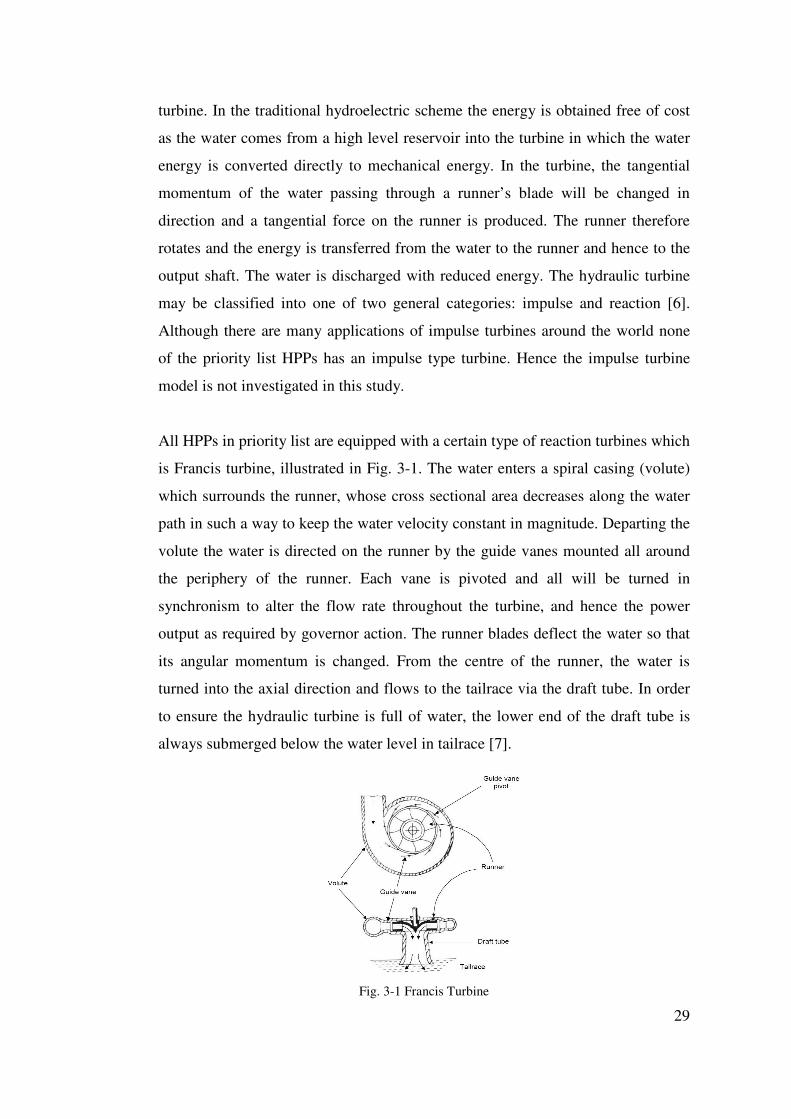
All HPPs in priority list are equipped with a certain type of reaction turbines which
is Francis turbine, illustrated in Fig. 3-1. The water enters a spiral casing (volute)
which surrounds the runner, whose cross sectional area decreases along the water
path in such a way to keep the water velocity constant in magnitude. Departing the
volute the water is directed on the runner by the guide vanes mounted all around
the periphery of the runner. Each vane is pivoted and all will be turned in
synchronism to alter the flow rate throughout the turbine, and hence the power
output as required by governor action. The runner blades deflect the water so that
its angular momentum is changed. From the centre of the runner, the water is
turned into the axial direction and flows to the tailrace via the draft tube. In order
to ensure the hydraulic turbine is full of water, the lower end of the draft tube is
always submerged below the water level in tailrace [7].
Fig. 3-1 Francis Turbine
30
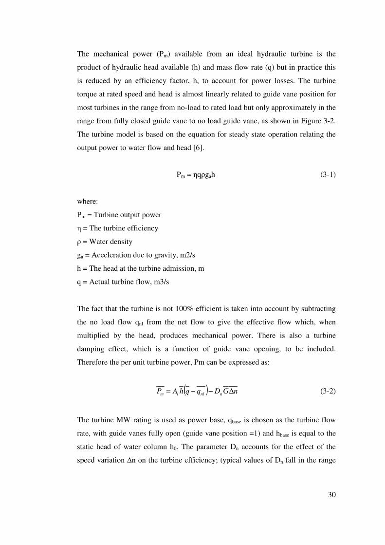
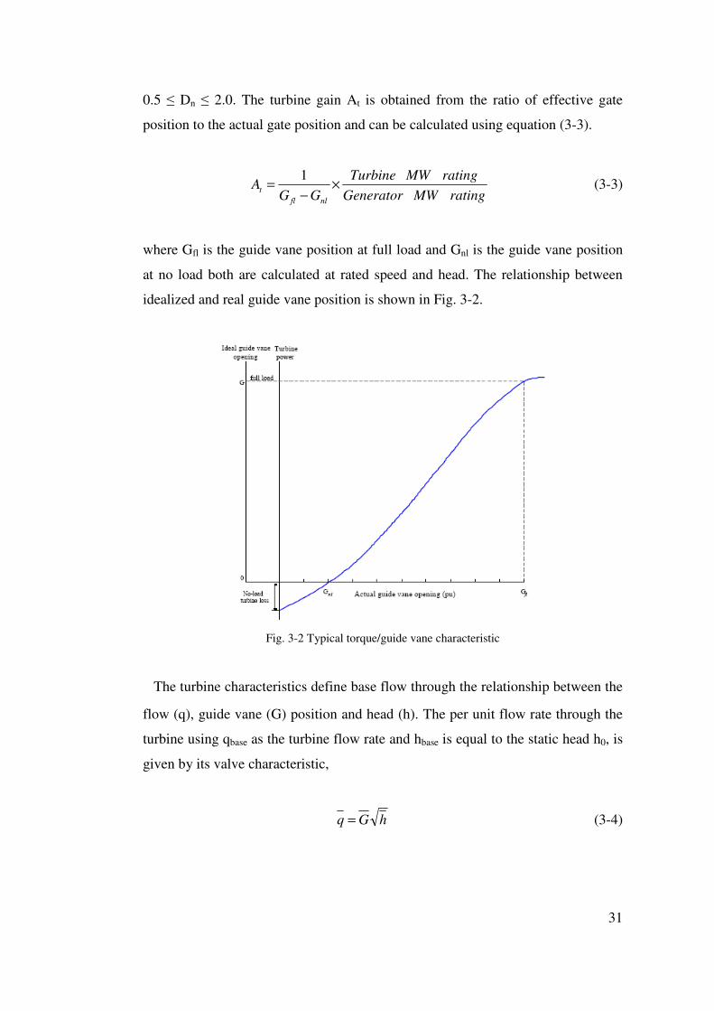
The mechanical power (Pm) available from an ideal hydraulic turbine is the
product of hydraulic head available (h) and mass flow rate (q) but in practice this
is reduced by an efficiency factor, h, to account for power losses. The turbine
torque at rated speed and head is almost linearly related to guide vane position for
most turbines in the range from no-load to rated load but only approximately in the
range from fully closed guide vane to no load guide vane, as shown in Figure 3-2.
The turbine model is based on the equation for steady state operation relating the
output power to water flow and head [6].
Pm = ηqρgah (3-1)
where:
Pm = Turbine output power
η = The turbine efficiency
ρ = Water density
ga = Acceleration due to gravity, m2/s
h = The head at the turbine admission, m
q = Actual turbine flow, m3/s
The fact that the turbine is not 100% efficient is taken into account by subtracting
the no load flow qnl from the net flow to give the effective flow which, when
multiplied by the head, produces mechanical power. There is also a turbine
damping effect, which is a function of guide vane opening, to be included.
Therefore the per unit turbine power, Pm can be expressed as:
( ) nGDqqhAP nnltm ∆−−= (3-2)
The turbine MW rating is used as power base, qbase is chosen as the turbine flow
rate, with guide vanes fully open (guide vane position =1) and hbase is equal to the
static head of water column h0. The parameter Dn accounts for the effect of the
speed variation ∆n on the turbine efficiency; typical values of Dn fall in the range
31
0.5 ≤ Dn ≤ 2.0. The turbine gain At is obtained from the ratio of effective gate
position to the actual gate position and can be calculated using equation (3-3).
ratingMWGenerator
ratingMWTurbine
GGA
nlfl
t ×−
=1
(3-3)
where Gfl is the guide vane position at full load and Gnl is the guide vane position
at no load both are calculated at rated speed and head. The relationship between
idealized and real guide vane position is shown in Fig. 3-2.
Fig. 3-2 Typical torque/guide vane characteristic
The turbine characteristics define base flow through the relationship between the
flow (q), guide vane (G) position and head (h). The per unit flow rate through the
turbine using qbase as the turbine flow rate and hbase is equal to the static head h0, is
given by its valve characteristic,
hGq = (3-4)

32
3.2.1.2. Modeling the Water Column The performance of a hydraulic turbine is greatly influenced by the characteristics
of the water column which feeds it, including the effect of water inertia in the
penstock. The effect of water inertia is to cause changes in turbine flow to lag
behind changes in the guide vane opening. In fact, the power has a transient
response which is initially in the opposite sense to that intended by changing the
guide vane position. Although the turbine guide vane opening may change rapidly,
the water column inertia prevents the flow from changing as rapidly.
Consequently, after a rapid increase in guide vane opening, and before the flow
has had time to change appreciably, the velocity of water into the wheel drops
because of the increased area of the guide vane opening. The power transfer to the
wheel actually drops before it increases to its required steady state value. This is
the most prominent factor, which makes a hydraulic turbine such an uncooperative
component in a speed control system [9].
The turbine and penstock characteristics are determined by three basic equations
relating to the velocity of water in the penstock, acceleration of the water column
under the influence of gravity and the production of mechanical power in the
turbine. First, a non-linear representation is developed which is appropriate when
large changes in speed and power are to be considered, such as in islanding, load
rejection and system restoration studies.
The basic water column model represents a single penstock with a very large or no
surge tank. The penstock is modeled on the assumption that the water acts as an
incompressible fluid so that here the water hammer effect may be neglected.
Consider here a rigid conduit of length l and cross-section area A, where the
penstock head losses hf due to the friction of water against the penstock wall are
proportional to flow (q) squared.
hf= fp q2 (3-5)
33
where fp, is the head loss coefficient in the penstock due to friction [10]. Assuming
that the water in the penstock can be treated approximately as a solid mass, the rate
of change of flow can be related to the head of water using Newton’s 2nd law of
motion. The force on the water mass is
( )dt
dvAlAghhh af ρρ =−−0 (3-6)
where
h0 = The static head of water column, m
h = The head at the turbine admission, m
hf = The head loss due to friction, m
fp = head loss coefficient, m/(m3/s)2
v = The water velocity, m/s
The rate of change of the flow in the penstock can be determined as:
( )l
Aghhh
dt
dq af−−= 0 (3-7)
Equation (3-7) can be written in per unit form in order to normalize system
representation. Compared to the use of physical units, the per unit format offers
computational simplicity by eliminating units and expressing the system quantities
as dimensionless ratios. The base values are chosen so that the principle variables
will be equal to one per unit under rated conditions. Here the base head hbase is
chosen to be the available static head h0 which is equal to the reservoir head minus
the tailrace head, and the base flow qbase is equal to the turbine flow with guide
vane fully open. Expressing equation (3-7) in per unit yields
( )base
abasef
lq
Aghhh
dt
qd−−= 1 (3-8)
( )w
f
T
hh
dt
qd −−=
1 (3-9)

34
where abase
base
abase
basew
gh
lv
Agh
lqT == is the water starting time.
The water starting time represents the time required for a head hbase to accelerate
the water in the penstock from standstill to the velocity vbase. This is calculated
between turbine inlet and the forebay or the surge tank if a large one exists [11].
Consider a simple penstock supplied from an open reservoir discharging into the
atmosphere as shown in Fig. 3-3. Opening the guide vane in a time ∆t causes the
velocity of the water in the penstock to increase by ∆v and the head at the turbine
inlet to drop by ∆h.
Fig. 3-3 Schematic of a HPP
The acceleration of water due to change in head at the turbine, characterized by
Newton’s
2nd law of motion may be expressed as
hAgdt
vdAl a ∆−=
∆ρρ (3-10)
The acceleration equation can be converted to per unit form by dividing by vbase
and hbase to give:
35
hdt
vd
hg
lv
basea
base ∆−=∆
(3-11)
Writing in terms of per unit variables
hdt
vdTw ∆−=
∆ (3-12)
This equation represents an important characteristic of the hydraulic plant.
Inspection of equation (3-12) shows that, if the guide vane is closed, a back
pressure will arise causing the water to decelerate. That is, if there is a positive
pressure change, there will be a negative acceleration change. Similarly, a negative
pressure change will cause a positive acceleration change. The maximum
acceleration occurs immediately after the guide vane opening because the entire
difference in pressure is available for accelerating the water. For a non-uniform
penstock with different cross sectional areas, the water inertia time constant is
calculated as [12]:
hg
lvT
a
w
∑= (3-13)
where ∑lv is the summation of length and velocity of sections in the water
passage.
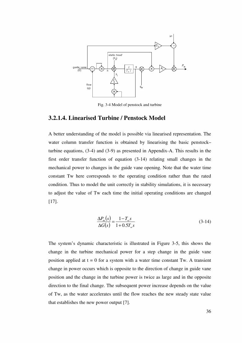
3.2.1.3. Combined Turbine / Penstock Model The hydraulic system can be modeled by combining equations (3-2) for the turbine
and (3-9) for the inelastic water column. The block diagram of Fig. 3-4 is a
nonlinear representation showing how the generated power depends on the guide
vane position. Note that the power also depends on additional inputs ∆n, h0 and qnl
but that these change slowly compared to the primary control input. The value for
water starting time of the penstock (Tw) is obtained at rated conditions using rated
head and rated flow as the base values.
36
Fig. 3-4 Model of penstock and turbine
3.2.1.4. Linearised Turbine / Penstock Model
A better understanding of the model is possible via linearised representation. The
water column transfer function is obtained by linearising the basic penstock–
turbine equations, (3-4) and (3-9) as presented in Appendix-A. This results in the
first order transfer function of equation (3-14) relating small changes in the
mechanical power to changes in the guide vane opening. Note that the water time
constant Tw here corresponds to the operating condition rather than the rated
condition. Thus to model the unit correctly in stability simulations, it is necessary
to adjust the value of Tw each time the initial operating conditions are changed
[17].
( )( ) sT
sT
sG
sP
w
wm
5.01
1
+
−=
∆
∆ (3-14)
The system’s dynamic characteristic is illustrated in Figure 3-5, this shows the
change in the turbine mechanical power for a step change in the guide vane
position applied at t = 0 for a system with a water time constant Tw. A transient
change in power occurs which is opposite to the direction of change in guide vane
position and the change in the turbine power is twice as large and in the opposite
direction to the final change. The subsequent power increase depends on the value
of Tw, as the water accelerates until the flow reaches the new steady state value
that establishes the new power output [7].
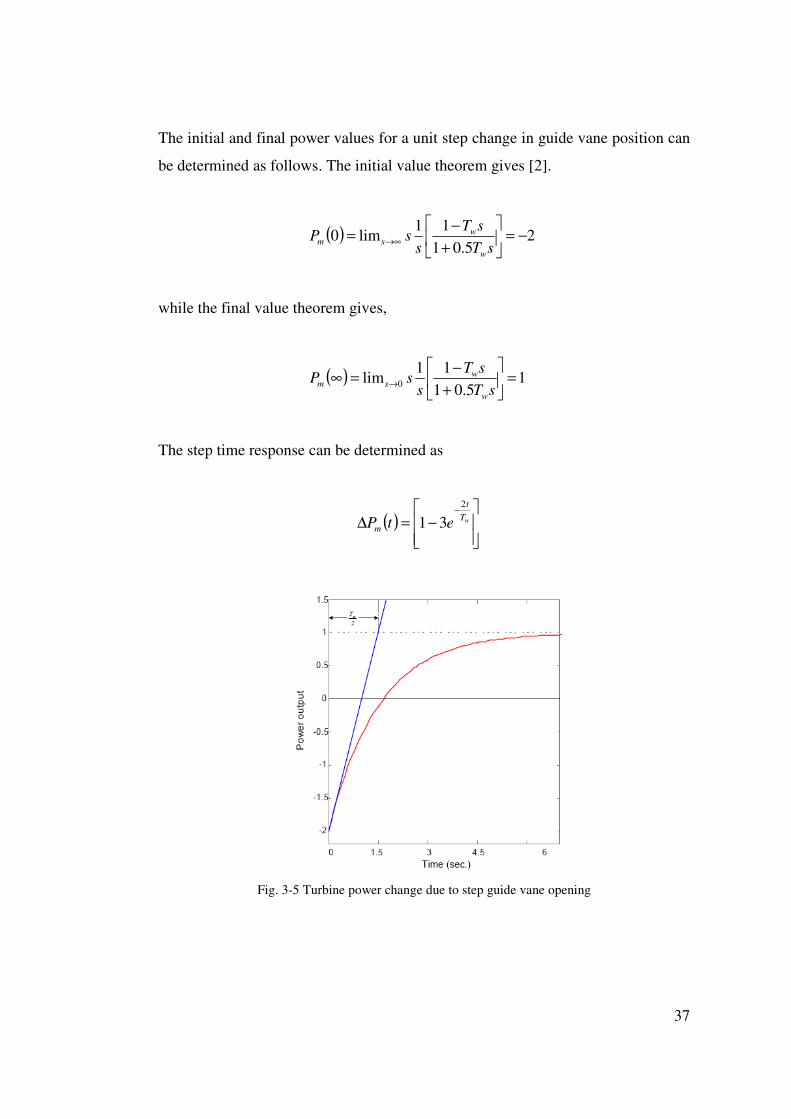
37
The initial and final power values for a unit step change in guide vane position can
be determined as follows. The initial value theorem gives [2].
( ) 25.01
11lim0 −=
+
−= →∞
sT
sT
ssP
w
wsm
while the final value theorem gives,
( ) 15.01
11lim 0 =
+
−=∞ →
sT
sT
ssP
w
wsm
The step time response can be determined as
( )
−=∆
−wT
t
m etP
2
31
Fig. 3-5 Turbine power change due to step guide vane opening
38
Generator Mechanical Model
The dynamic behavior of the generators within a power system is of fundamental
importance to the overall quality of the power supply. The synchronous generator
converts mechanical power to electrical power at a specific voltage and frequency.
The source of the mechanical power, the prime mover, may be a diesel engine, a
steam turbine or a water turbine. Whatever the source, it must have the basic
property that its speed is almost constant regardless of the power demand. The
analysis of any power system to determine its long term frequency stability
involves the mechanical properties of the machines.
The mechanical equations of a rotating machine are very well established and they
are based on the swing equation of the rotating inertia. The equation is based on
the elementary principle in dynamics which states that accelerating torque is the
product of moment of inertia of the rotor times its angular acceleration. [14].
Constant shaft speed for a given machine is maintained when there is equilibrium
between the mechanical shaft and electrical torques. Any imbalance between the
torques will cause the acceleration or deceleration of the machine according to the
equation (3-14).
elecmechm
acc TTdt
dJT −==
2
2δ (3-14)
where:
Tacc = Accelerating torque, N.m.
J = Combined moment of inertia of the generator and turbine, Kg.m2
δm = Mechanical torque angle of the rotor, rad.
t = Time, seconds
Tmech = Mechanical torque, N.m.
Telec = Electromagnetic torque, N.m
The mechanical angular velocity ωm is the time derivative of the torque angle.
Rewriting
(3-14) yields,
39
elecmechm TT
dt
dJ −=
ω (3-15)
The kinetic energy of a rotating body is equal to ½ J ωm2, thus equation (3-15) can
be normalized in terms of the per unit inertia constant H, which is defined as the
kinetic energy of the machine at rated speed per machine volt-ampere rating.
Using wm0 to denote rated angular velocity in mechanical radians per second gives
elecmechm
m
base TTdt
dHVA−=
ω
ω 20
2 (3-16)
The angular velocity of the rotor in electric rad/sec ω is related to the rotor
mechanical angular velocity by n
m
p
ωω = , where Pn is the number of generator
poles. The equation of motion in per unit form can be written using the angular
velocity of the rotor in electric rad/sec.
elecmech TTdt
dH −=
ω2 (3-17)
where 0m
basebase
VAT
ω=
It is preferable to express the relationship of equation (3-17) in term of mechanical
and electrical power rather than torque. Since the power is equal to torque times
angular velocity, P=Tω, expanding for small oscillations around the operating
point and neglecting the second order terms gives,
ωω ∆+∆=∆ 0TTP o (3-18)
At steady state, the mechanical torque is equal to the electrical torque (Tmec0
≅ Telec0). Combining equations (3-17) and (3-18), the deviation in per unit speed
40
∆ω of the rotor as a function of deviations in the mechanical and electrical powers
can be represented as
ω∆=∆−∆ HsPP em 2 (3-19)
3.2.1.5. Mechanical Starting Time
The mechanical starting time of the machine Tm, can be calculated using equation
(3-17) where,
H
T
dt
d acc
2=
ω
Let Tm be the time required by the rated torque to accelerate the rotor from stand
still to rated speed. Integrating with respect to time with ω = 1.0 pu, and Tacc = 1.0
pu results in:
∫=mT
dtH
0
12
11
Therefore, the mechanical starting time Tm = 2H
Speed Controller Models
The frequency of a power system is dependent on the balance between the
generated and demanded power. In case of an imbalance the difference should be
eliminated by the controllers in each plant according to their speed droop settings,
which is referred as primary control as previously explained
The primary speed control function involves feeding back speed error to control
the gate position. In order to ensure satisfactory and stable parallel operation of
multiple units, the speed controller is provided with a droop characteristic as
discussed in previous chapters. Fig. 2-7 also indicates the schematic of a speed
controller with speed-droop characteristic.
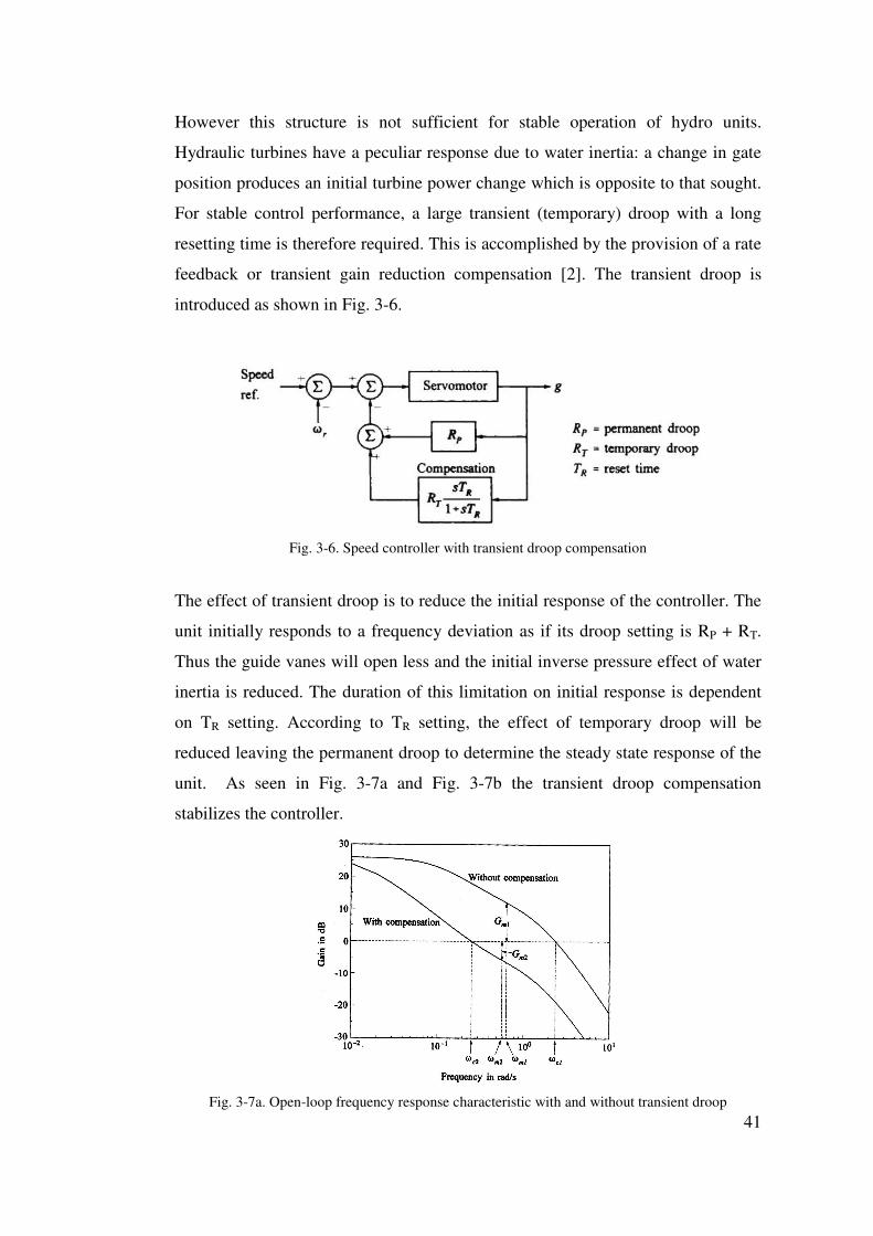
41
However this structure is not sufficient for stable operation of hydro units.
Hydraulic turbines have a peculiar response due to water inertia: a change in gate
position produces an initial turbine power change which is opposite to that sought.
For stable control performance, a large transient (temporary) droop with a long
resetting time is therefore required. This is accomplished by the provision of a rate
feedback or transient gain reduction compensation [2]. The transient droop is
introduced as shown in Fig. 3-6.
Fig. 3-6. Speed controller with transient droop compensation
The effect of transient droop is to reduce the initial response of the controller. The
unit initially responds to a frequency deviation as if its droop setting is RP + RT.
Thus the guide vanes will open less and the initial inverse pressure effect of water
inertia is reduced. The duration of this limitation on initial response is dependent
on TR setting. According to TR setting, the effect of temporary droop will be
reduced leaving the permanent droop to determine the steady state response of the
unit. As seen in Fig. 3-7a and Fig. 3-7b the transient droop compensation
stabilizes the controller.
Fig. 3-7a. Open-loop frequency response characteristic with and without transient droop
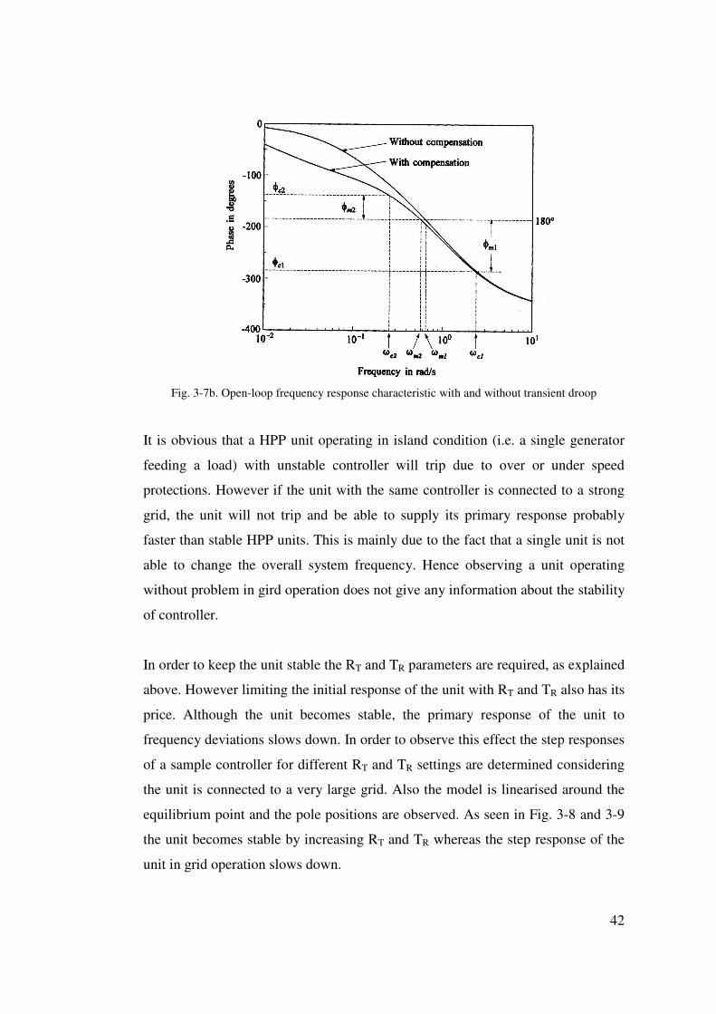
42
Fig. 3-7b. Open-loop frequency response characteristic with and without transient droop
It is obvious that a HPP unit operating in island condition (i.e. a single generator
feeding a load) with unstable controller will trip due to over or under speed
protections. However if the unit with the same controller is connected to a strong
grid, the unit will not trip and be able to supply its primary response probably
faster than stable HPP units. This is mainly due to the fact that a single unit is not
able to change the overall system frequency. Hence observing a unit operating
without problem in gird operation does not give any information about the stability
of controller.
In order to keep the unit stable the RT and TR parameters are required, as explained
above. However limiting the initial response of the unit with RT and TR also has its
price. Although the unit becomes stable, the primary response of the unit to
frequency deviations slows down. In order to observe this effect the step responses
of a sample controller for different RT and TR settings are determined considering
the unit is connected to a very large grid. Also the model is linearised around the
equilibrium point and the pole positions are observed. As seen in Fig. 3-8 and 3-9
the unit becomes stable by increasing RT and TR whereas the step response of the
unit in grid operation slows down.
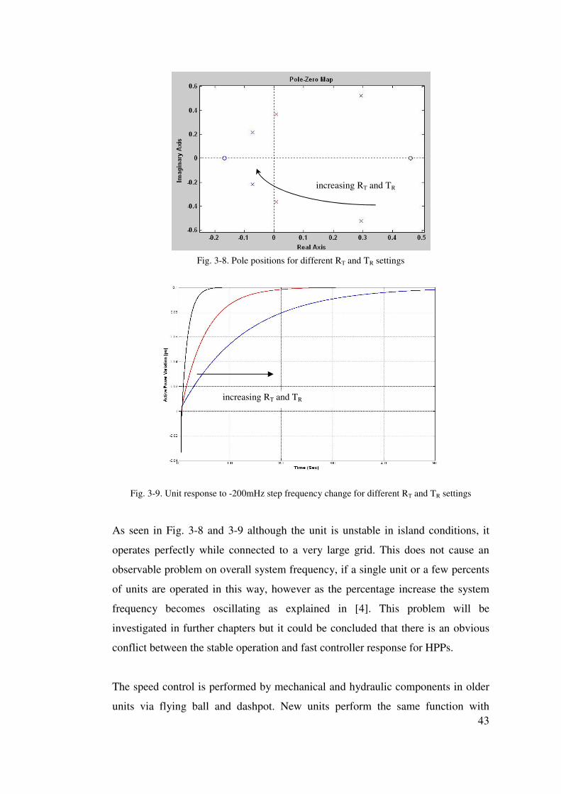
43
Fig. 3-8. Pole positions for different RT and TR settings
Fig. 3-9. Unit response to -200mHz step frequency change for different RT and TR settings
As seen in Fig. 3-8 and 3-9 although the unit is unstable in island conditions, it
operates perfectly while connected to a very large grid. This does not cause an
observable problem on overall system frequency, if a single unit or a few percents
of units are operated in this way, however as the percentage increase the system
frequency becomes oscillating as explained in [4]. This problem will be
investigated in further chapters but it could be concluded that there is an obvious
conflict between the stable operation and fast controller response for HPPs.
The speed control is performed by mechanical and hydraulic components in older
units via flying ball and dashpot. New units perform the same function with
increasing RT and TR
increasing RT and TR
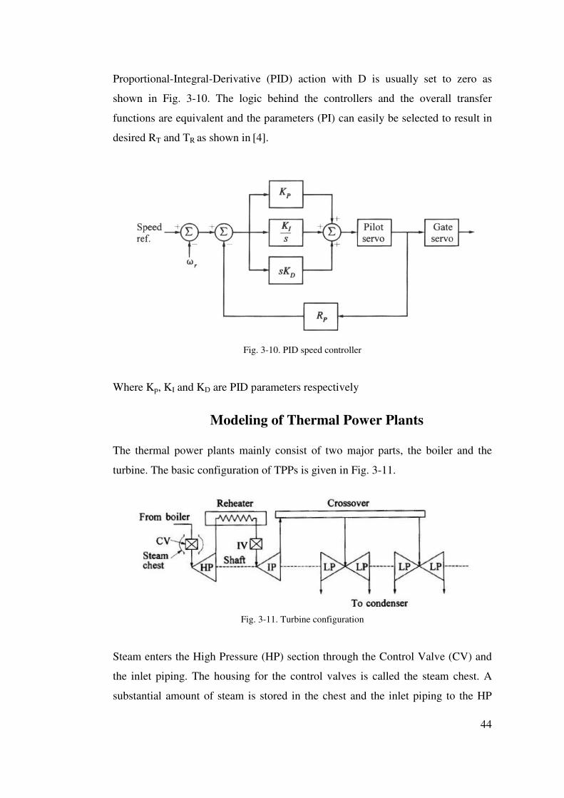
44
Proportional-Integral-Derivative (PID) action with D is usually set to zero as
shown in Fig. 3-10. The logic behind the controllers and the overall transfer
functions are equivalent and the parameters (PI) can easily be selected to result in
desired RT and TR as shown in [4].
Fig. 3-10. PID speed controller
Where Kp, KI and KD are PID parameters respectively
3.3. Modeling of Thermal Power Plants The thermal power plants mainly consist of two major parts, the boiler and the
turbine. The basic configuration of TPPs is given in Fig. 3-11.
Fig. 3-11. Turbine configuration
Steam enters the High Pressure (HP) section through the Control Valve (CV) and
the inlet piping. The housing for the control valves is called the steam chest. A
substantial amount of steam is stored in the chest and the inlet piping to the HP
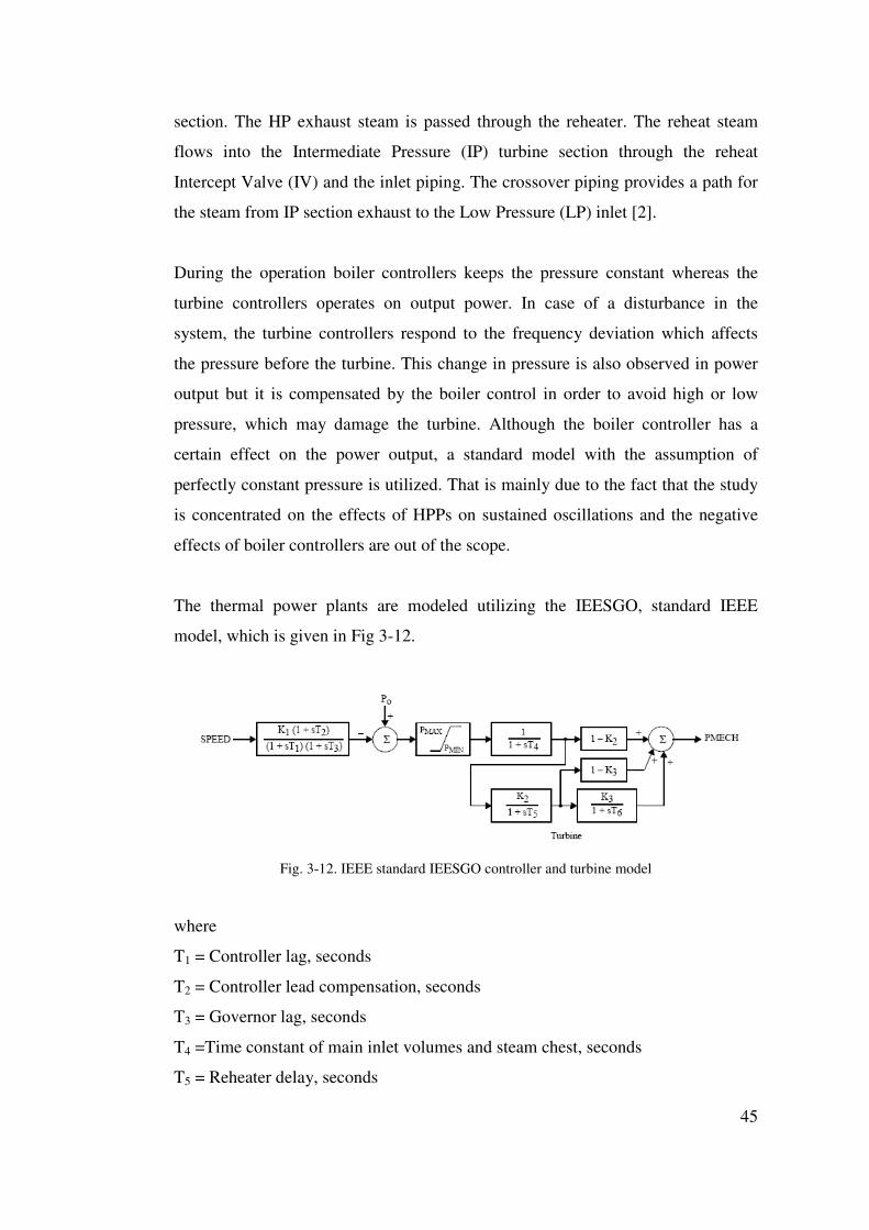
45
section. The HP exhaust steam is passed through the reheater. The reheat steam
flows into the Intermediate Pressure (IP) turbine section through the reheat
Intercept Valve (IV) and the inlet piping. The crossover piping provides a path for
the steam from IP section exhaust to the Low Pressure (LP) inlet [2].
During the operation boiler controllers keeps the pressure constant whereas the
turbine controllers operates on output power. In case of a disturbance in the
system, the turbine controllers respond to the frequency deviation which affects
the pressure before the turbine. This change in pressure is also observed in power
output but it is compensated by the boiler control in order to avoid high or low
pressure, which may damage the turbine. Although the boiler controller has a
certain effect on the power output, a standard model with the assumption of
perfectly constant pressure is utilized. That is mainly due to the fact that the study
is concentrated on the effects of HPPs on sustained oscillations and the negative
effects of boiler controllers are out of the scope.
The thermal power plants are modeled utilizing the IEESGO, standard IEEE
model, which is given in Fig 3-12.
Fig. 3-12. IEEE standard IEESGO controller and turbine model
where
T1 = Controller lag, seconds
T2 = Controller lead compensation, seconds
T3 = Governor lag, seconds
T4 =Time constant of main inlet volumes and steam chest, seconds
T5 = Reheater delay, seconds
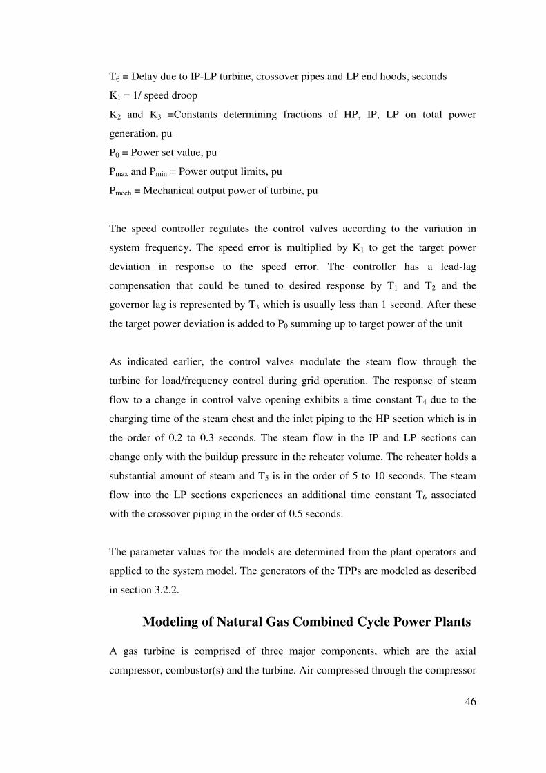
46
T6 = Delay due to IP-LP turbine, crossover pipes and LP end hoods, seconds
K1 = 1/ speed droop
K2 and K3 =Constants determining fractions of HP, IP, LP on total power
generation, pu
P0 = Power set value, pu
Pmax and Pmin = Power output limits, pu
Pmech = Mechanical output power of turbine, pu
The speed controller regulates the control valves according to the variation in
system frequency. The speed error is multiplied by K1 to get the target power
deviation in response to the speed error. The controller has a lead-lag
compensation that could be tuned to desired response by T1 and T2 and the
governor lag is represented by T3 which is usually less than 1 second. After these
the target power deviation is added to P0 summing up to target power of the unit
As indicated earlier, the control valves modulate the steam flow through the
turbine for load/frequency control during grid operation. The response of steam
flow to a change in control valve opening exhibits a time constant T4 due to the
charging time of the steam chest and the inlet piping to the HP section which is in
the order of 0.2 to 0.3 seconds. The steam flow in the IP and LP sections can
change only with the buildup pressure in the reheater volume. The reheater holds a
substantial amount of steam and T5 is in the order of 5 to 10 seconds. The steam
flow into the LP sections experiences an additional time constant T6 associated
with the crossover piping in the order of 0.5 seconds.
The parameter values for the models are determined from the plant operators and
applied to the system model. The generators of the TPPs are modeled as described
in section 3.2.2.
3.4. Modeling of Natural Gas Combined Cycle Power Plants A gas turbine is comprised of three major components, which are the axial
compressor, combustor(s) and the turbine. Air compressed through the compressor
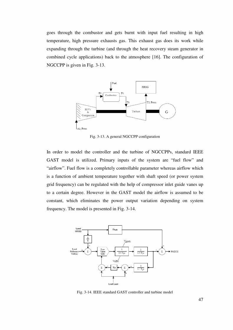
47
goes through the combustor and gets burnt with input fuel resulting in high
temperature, high pressure exhausts gas. This exhaust gas does its work while
expanding through the turbine (and through the heat recovery steam generator in
combined cycle applications) back to the atmosphere [16]. The configuration of
NGCCPP is given in Fig. 3-13.
Fig. 3-13. A general NGCCPP configuration
In order to model the controller and the turbine of NGCCPPs, standard IEEE
GAST model is utilized. Primary inputs of the system are “fuel flow” and
“airflow”. Fuel flow is a completely controllable parameter whereas airflow which
is a function of ambient temperature together with shaft speed (or power system
grid frequency) can be regulated with the help of compressor inlet guide vanes up
to a certain degree. However in the GAST model the airflow is assumed to be
constant, which eliminates the power output variation depending on system
frequency. The model is presented in Fig. 3-14.
Fig. 3-14. IEEE standard GAST controller and turbine model
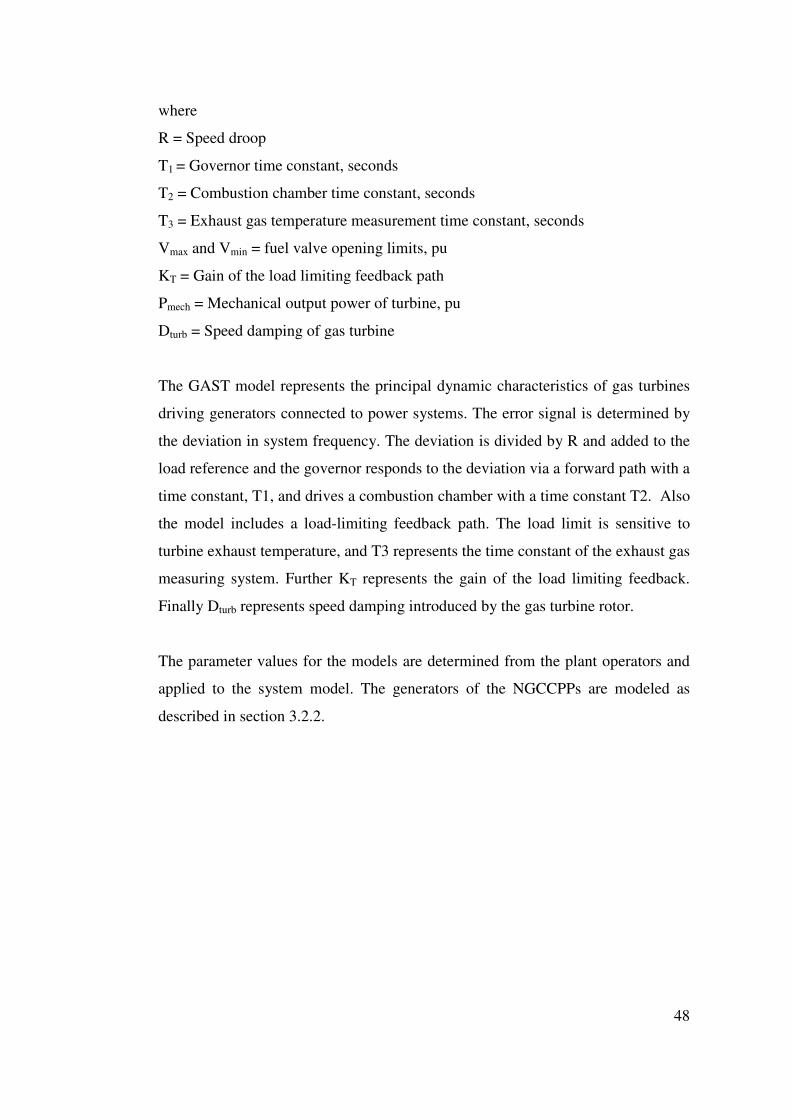
48
where
R = Speed droop
T1 = Governor time constant, seconds
T2 = Combustion chamber time constant, seconds
T3 = Exhaust gas temperature measurement time constant, seconds
Vmax and Vmin = fuel valve opening limits, pu
KT = Gain of the load limiting feedback path
Pmech = Mechanical output power of turbine, pu
Dturb = Speed damping of gas turbine
The GAST model represents the principal dynamic characteristics of gas turbines
driving generators connected to power systems. The error signal is determined by
the deviation in system frequency. The deviation is divided by R and added to the
load reference and the governor responds to the deviation via a forward path with a
time constant, T1, and drives a combustion chamber with a time constant T2. Also
the model includes a load-limiting feedback path. The load limit is sensitive to
turbine exhaust temperature, and T3 represents the time constant of the exhaust gas
measuring system. Further KT represents the gain of the load limiting feedback.
Finally Dturb represents speed damping introduced by the gas turbine rotor.
The parameter values for the models are determined from the plant operators and
applied to the system model. The generators of the NGCCPPs are modeled as
described in section 3.2.2.

49
C H A P T E R 4
4. MODELING AND SIMULATION STUDIES
4.1. Introduction
After describing the dynamical behavior of power plants focusing on the HPPs,
this chapter proceeds with the results of performed field tests on speed controllers.
During the visit of experts from UCTE to Turkey, two island operations tests were
performed in Birecik and Atatürk HPPs in order to observe the ability of plants to
operate in island mode. Both tests resulted in unit trips. The theoretical studies
indicated that the unit trips were due to unstable operational settings of the plants.
This chapter describes the theoretical studies performed in order to determine the
model and the effects of controller parameters on stability of the unit.
As the data of other major HPPs are acquired from plant operators, the simulations
indicated that most of the HPPs are operating with unstable settings. In order to
observe the effects of HPPs with unstable settings on power system frequency, the
power system model to analyze the long term frequency stability is determined.
The derivations regarding the model are also given in this chapter. After
determination, the model is verified by measurements of real events. Having the
model validated, the effects of changes on governor settings are simulated and
results are presented further in this chapter.
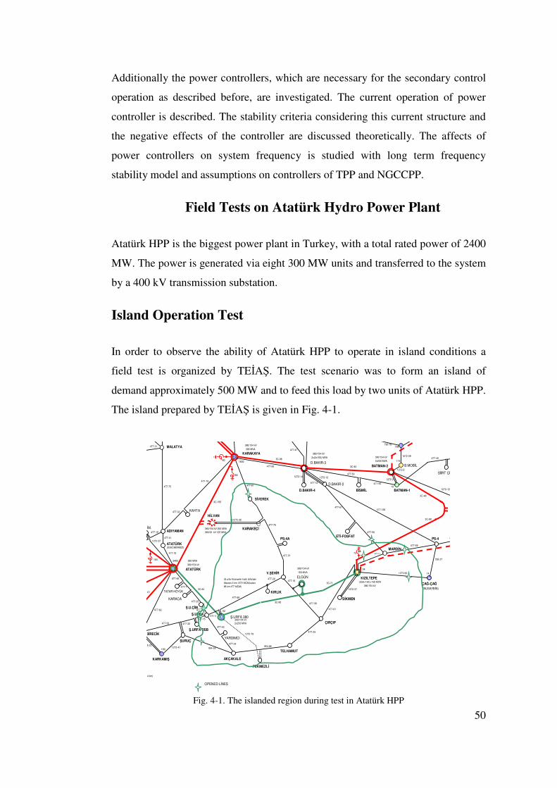
50
Additionally the power controllers, which are necessary for the secondary control
operation as described before, are investigated. The current operation of power
controller is described. The stability criteria considering this current structure and
the negative effects of the controller are discussed theoretically. The affects of
power controllers on system frequency is studied with long term frequency
stability model and assumptions on controllers of TPP and NGCCPP.
4.2. Field Tests on Atatürk Hydro Power Plant
Atatürk HPP is the biggest power plant in Turkey, with a total rated power of 2400
MW. The power is generated via eight 300 MW units and transferred to the system
by a 400 kV transmission substation.
Island Operation Test
In order to observe the ability of Atatürk HPP to operate in island conditions a
field test is organized by TEİAŞ. The test scenario was to form an island of
demand approximately 500 MW and to feed this load by two units of Atatürk HPP.
The island prepared by TEİAŞ is given in Fig. 4-1.
Fig. 4-1. The islanded region during test in Atatürk HPP
MALATYA
KARAKAYA
D.BAKIR-4 BİSMİL BATMAN-1
HİLVAN
ADIYAMANKARAKEÇİ
PS-4AETİ-FOSFAT
PS-4
ATATÜRK
ATATÜRK
DİKMEN
Ş.U.ÇİM
Ş.URFA
ÇIRÇIP
YARDIMCI
TELHAMUT
AKÇAKALE
OPENED LİNES
PEKMEZLİ
SİVEREK
80
60
183
1800
2405
189
19
14
2x250 MVA
380/154 kV
300 MVA
380/154 kV
380/154 kV
300 MVA
2x(2x150) MVA
380/154 kV380/154 kV
2x250 MVA
BATMAN-2
3C-96
3C-93
3C-40
3C-80
3C-71
3C-642C-61
3C-155
477-47
477-93
1272-14 1272-12477-53
477-50
477-128477-61
477-50
477-59
1272-60
795-27
477-34
477-61
477-30
477-23
954-88477-34
477-20
477-61
477-79
477-76
477-31
477-32
477-75
477-15
1272-37477-41
477-7
477-13
1272-13
477-40
477-15
954-531272-41
477-56
795-22
477-21
477-17795-18
477-10
477-32
1272-39
1272-2
477-11
D.BAKIR-2477-12
198
34
118
B.MOBİL
1272-129
477-45
477-68
1272-2
1272-70
477-62
2x1272-35
380/154 kV 250 MVA380/33 kV 125 MVA
(ESKİ MERKEZ)
477-45
KARACA
TATAR HÖYÜK
477-25
KIRLIK
(Ş.urfa-Viranşehir hattı Urfa'dan itibaren 2 km 1272 MCM,kalanı 88 km 477 MCM)
1272-37380/154 kV
(250+150)+150 MVA
73
KARKAMIŞ
tamamı (124 km)
Ş.URFA 380
ŞURUÇ
SİİRT ÇİM
KIZILTEPE
KAHTA
Ş.URFA OSB
ADI.ÇİM.
MARDİN
BİRECİK
D.BAKIR-3
ÇAĞ-ÇAĞ(NUSAYBİN)
52
V.ŞEHİRELGÜN
380/154 kV
150 MVA
477-10
3C-90
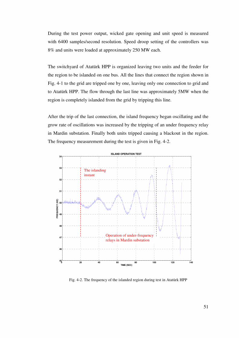
51
During the test power output, wicked gate opening and unit speed is measured
with 6400 samples/second resolution. Speed droop setting of the controllers was
8% and units were loaded at approximately 250 MW each.
The switchyard of Atatürk HPP is organized leaving two units and the feeder for
the region to be islanded on one bus. All the lines that connect the region shown in
Fig. 4-1 to the grid are tripped one by one, leaving only one connection to grid and
to Atatürk HPP. The flow through the last line was approximately 5MW when the
region is completely islanded from the grid by tripping this line.
After the trip of the last connection, the island frequency began oscillating and the
grow rate of oscillations was increased by the tripping of an under frequency relay
in Mardin substation. Finally both units tripped causing a blackout in the region.
The frequency measurement during the test is given in Fig. 4-2.
0 20 40 60 80 100 120 14045
46
47
48
49
50
51
52
53
54
TIME (SEC)
FR
EQ
UE
NC
Y (H
Z)
ISLAND OPERATION TEST
Fig. 4-2. The frequency of the islanded region during test in Atatürk HPP
The islanding instant
Operation of under-frequency relays in Mardin substation
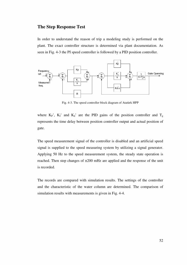
52
The Step Response Test
In order to understand the reason of trip a modeling study is performed on the
plant. The exact controller structure is determined via plant documentation. As
seen in Fig. 4-3 the PI speed controller is followed by a PID position controller.
Fig. 4-3. The speed controller block diagram of Atatürk HPP
where KP’, KI’ and Kd’ are the PID gains of the position controller and Tg
represents the time delay between position controller output and actual position of
gate.
The speed measurement signal of the controller is disabled and an artificial speed
signal is supplied to the speed measuring system by utilizing a signal generator.
Applying 50 Hz to the speed measurement system, the steady state operation is
reached. Then step changes of ±200 mHz are applied and the response of the unit
is recorded.
The records are compared with simulation results. The settings of the controller
and the characteristic of the water column are determined. The comparison of
simulation results with measurements is given in Fig. 4-4.
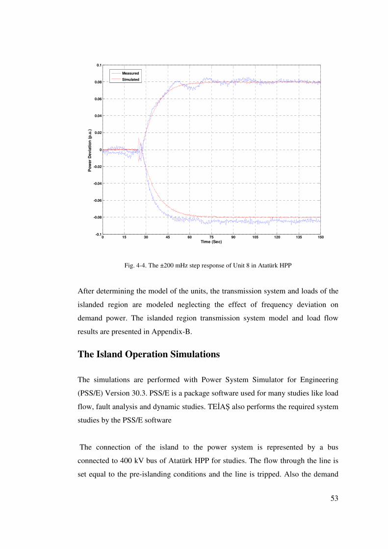
53
0 15 30 45 60 75 90 105 120 135 150-0.1
-0.08
-0.06
-0.04
-0.02
0
0.02
0.04
0.06
0.08
0.1
Time (Sec)
Po
wer
Dev
iati
on
(p
.u.)
Measured
Simulated
Fig. 4-4. The ±200 mHz step response of Unit 8 in Atatürk HPP
After determining the model of the units, the transmission system and loads of the
islanded region are modeled neglecting the effect of frequency deviation on
demand power. The islanded region transmission system model and load flow
results are presented in Appendix-B.
The Island Operation Simulations
The simulations are performed with Power System Simulator for Engineering
(PSS/E) Version 30.3. PSS/E is a package software used for many studies like load
flow, fault analysis and dynamic studies. TEİAŞ also performs the required system
studies by the PSS/E software
The connection of the island to the power system is represented by a bus
connected to 400 kV bus of Atatürk HPP for studies. The flow through the line is
set equal to the pre-islanding conditions and the line is tripped. Also the demand
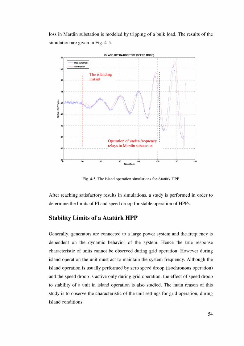
54
loss in Mardin substation is modeled by tripping of a bulk load. The results of the
simulation are given in Fig. 4-5.
0 20 40 60 80 100 120 14045
46
47
48
49
50
51
52
53
54
Time (Sec)
FR
EQ
UE
NC
Y (H
z)ISLAND OPERATION TEST (SPEED MODE)
Measurement
Simulation
Fig. 4-5. The island operation simulations for Atatürk HPP
After reaching satisfactory results in simulations, a study is performed in order to
determine the limits of PI and speed droop for stable operation of HPPs.
Stability Limits of a Atatürk HPP
Generally, generators are connected to a large power system and the frequency is
dependent on the dynamic behavior of the system. Hence the true response
characteristic of units cannot be observed during grid operation. However during
island operation the unit must act to maintain the system frequency. Although the
island operation is usually performed by zero speed droop (isochronous operation)
and the speed droop is active only during grid operation, the effect of speed droop
to stability of a unit in island operation is also studied. The main reason of this
study is to observe the characteristic of the unit settings for grid operation, during
island conditions.
The islanding instant
Operation of under-frequency relays in Mardin substation
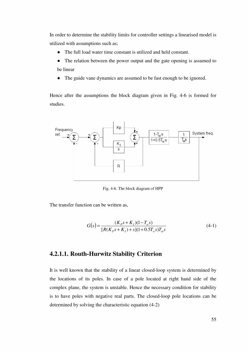
55
In order to determine the stability limits for controller settings a linearised model is
utilized with assumptions such as;
● The full load water time constant is utilized and held constant.
● The relation between the power output and the gate opening is assumed to
be linear
● The guide vane dynamics are assumed to be fast enough to be ignored.
Hence after the assumptions the block diagram given in Fig. 4-6 is formed for
studies.
Fig. 4-6. The block diagram of HPP
The transfer function can be written as,
( )sTsTsKsKR
sTKsKsG
mwIP
wIP
)5.01]()([
)1)((
+++
−+= (4-1)
4.2.1.1. Routh-Hurwitz Stability Criterion
It is well known that the stability of a linear closed-loop system is determined by
the locations of its poles. In case of a pole located at right hand side of the
complex plane, the system is unstable. Hence the necessary condition for stability
is to have poles with negative real parts. The closed-loop pole locations can be
determined by solving the characteristic equation (4-2)
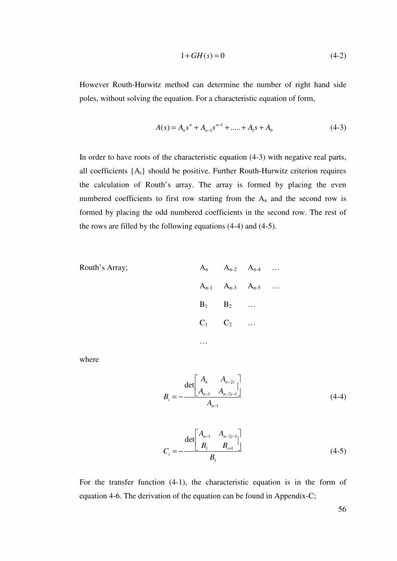
56
0)(1 =+ sGH (4-2)
However Routh-Hurwitz method can determine the number of right hand side
poles, without solving the equation. For a characteristic equation of form,
011
1 .....)( AsAsAsAsAn
n
n
n ++++= −
− (4-3)
In order to have roots of the characteristic equation (4-3) with negative real parts,
all coefficients {Ai} should be positive. Further Routh-Hurwitz criterion requires
the calculation of Routh’s array. The array is formed by placing the even
numbered coefficients to first row starting from the An and the second row is
formed by placing the odd numbered coefficients in the second row. The rest of
the rows are filled by the following equations (4-4) and (4-5).
Routh’s Array; An An-2 An-4 … An-1 An-3 An-5 … B1 B2 … C1 C2 … … where
1
121
2det
−
−−−
−
−=n
inn
inn
iA
AA
AA
B (4-4)
1
11
121det
B
BB
AA
Ci
inn
i
−= +
−−−
(4-5)
For the transfer function (4-1), the characteristic equation is in the form of
equation 4-6. The derivation of the equation can be found in Appendix-C;
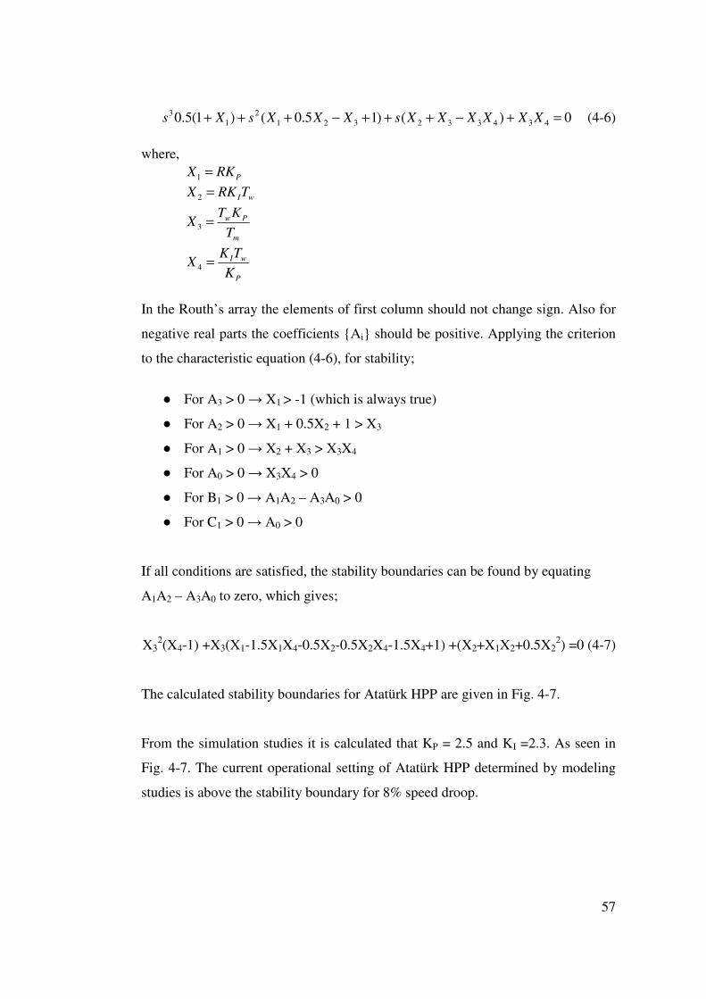
57
0)()15.0()1(5.0 4343323212
13 =+−+++−+++ XXXXXXsXXXsXs (4-6)
where,
PRKX =1
wITRKX =2
m
Pw
T
KTX =3
P
wI
K
TKX =4
In the Routh’s array the elements of first column should not change sign. Also for
negative real parts the coefficients {Ai} should be positive. Applying the criterion
to the characteristic equation (4-6), for stability;
● For A3 > 0 → X1 > -1 (which is always true)
● For A2 > 0 → X1 + 0.5X2 + 1 > X3
● For A1 > 0 → X2 + X3 > X3X4
● For A0 > 0 → X3X4 > 0
● For B1 > 0 → A1A2 – A3A0 > 0
● For C1 > 0 → A0 > 0
If all conditions are satisfied, the stability boundaries can be found by equating
A1A2 – A3A0 to zero, which gives;
X32(X4-1) +X3(X1-1.5X1X4-0.5X2-0.5X2X4-1.5X4+1) +(X2+X1X2+0.5X2
2) =0 (4-7)
The calculated stability boundaries for Atatürk HPP are given in Fig. 4-7.
From the simulation studies it is calculated that KP = 2.5 and KI =2.3. As seen in
Fig. 4-7. The current operational setting of Atatürk HPP determined by modeling
studies is above the stability boundary for 8% speed droop.
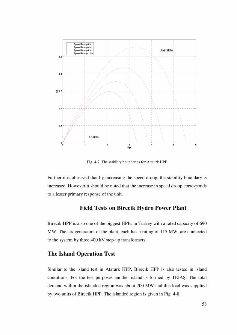
58
0 1 2 3 4 5 60
0.1
0.2
0.3
0.4
0.5
Kp
KI
Speed Droop 0%Speed Droop 4%Speed Droop 8%Speed Droop 12%
Unstable
Stable
Fig. 4-7. The stability boundaries for Atatürk HPP
Further it is observed that by increasing the speed droop, the stability boundary is
increased. However it should be noted that the increase in speed droop corresponds
to a lesser primary response of the unit.
4.3. Field Tests on Birecik Hydro Power Plant
Birecik HPP is also one of the biggest HPPs in Turkey with a rated capacity of 690
MW. The six generators of the plant, each has a rating of 115 MW, are connected
to the system by three 400 kV step-up transformers.
The Island Operation Test
Similar to the island test in Atatürk HPP, Birecik HPP is also tested in island
conditions. For the test purposes another island is formed by TEİAŞ. The total
demand within the islanded region was about 200 MW and this load was supplied
by two units of Birecik HPP. The islanded region is given in Fig. 4-8.
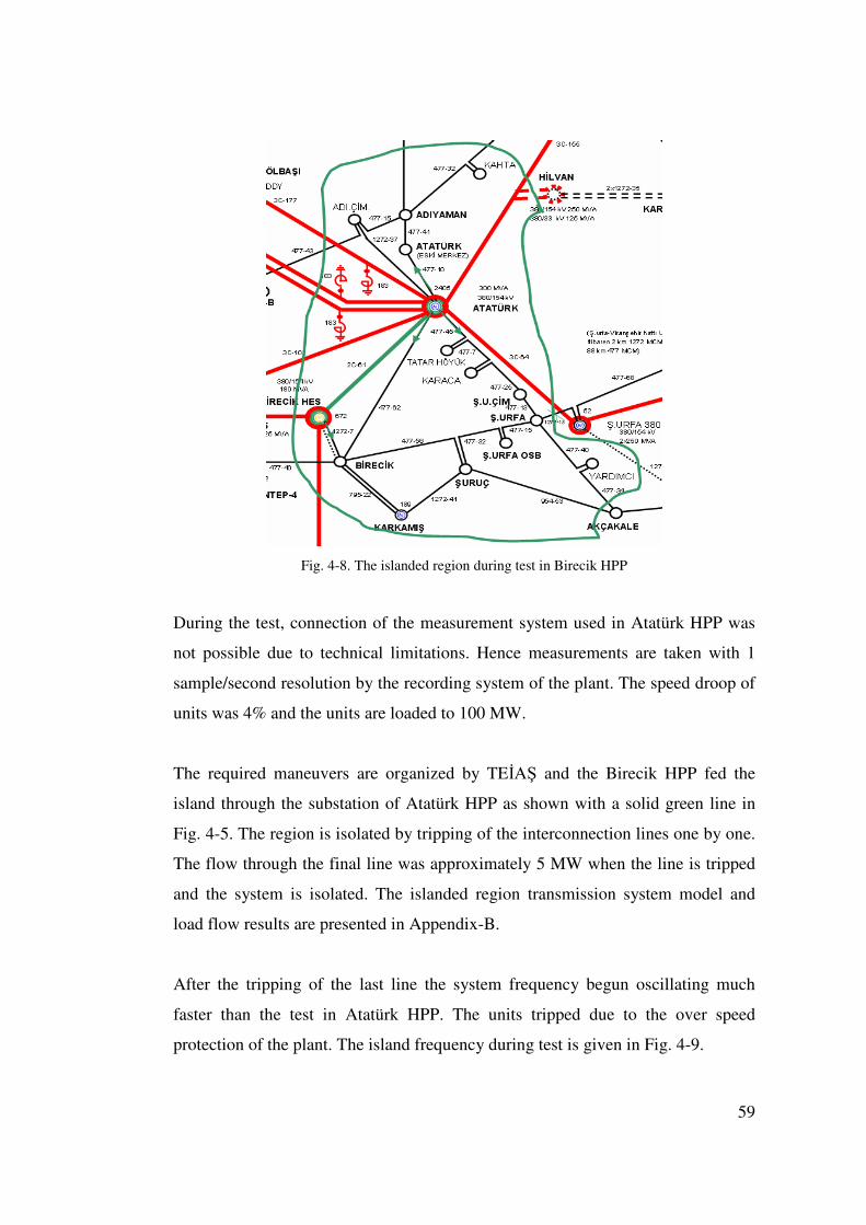
59
Fig. 4-8. The islanded region during test in Birecik HPP
During the test, connection of the measurement system used in Atatürk HPP was
not possible due to technical limitations. Hence measurements are taken with 1
sample/second resolution by the recording system of the plant. The speed droop of
units was 4% and the units are loaded to 100 MW.
The required maneuvers are organized by TEİAŞ and the Birecik HPP fed the
island through the substation of Atatürk HPP as shown with a solid green line in
Fig. 4-5. The region is isolated by tripping of the interconnection lines one by one.
The flow through the final line was approximately 5 MW when the line is tripped
and the system is isolated. The islanded region transmission system model and
load flow results are presented in Appendix-B.
After the tripping of the last line the system frequency begun oscillating much
faster than the test in Atatürk HPP. The units tripped due to the over speed
protection of the plant. The island frequency during test is given in Fig. 4-9.
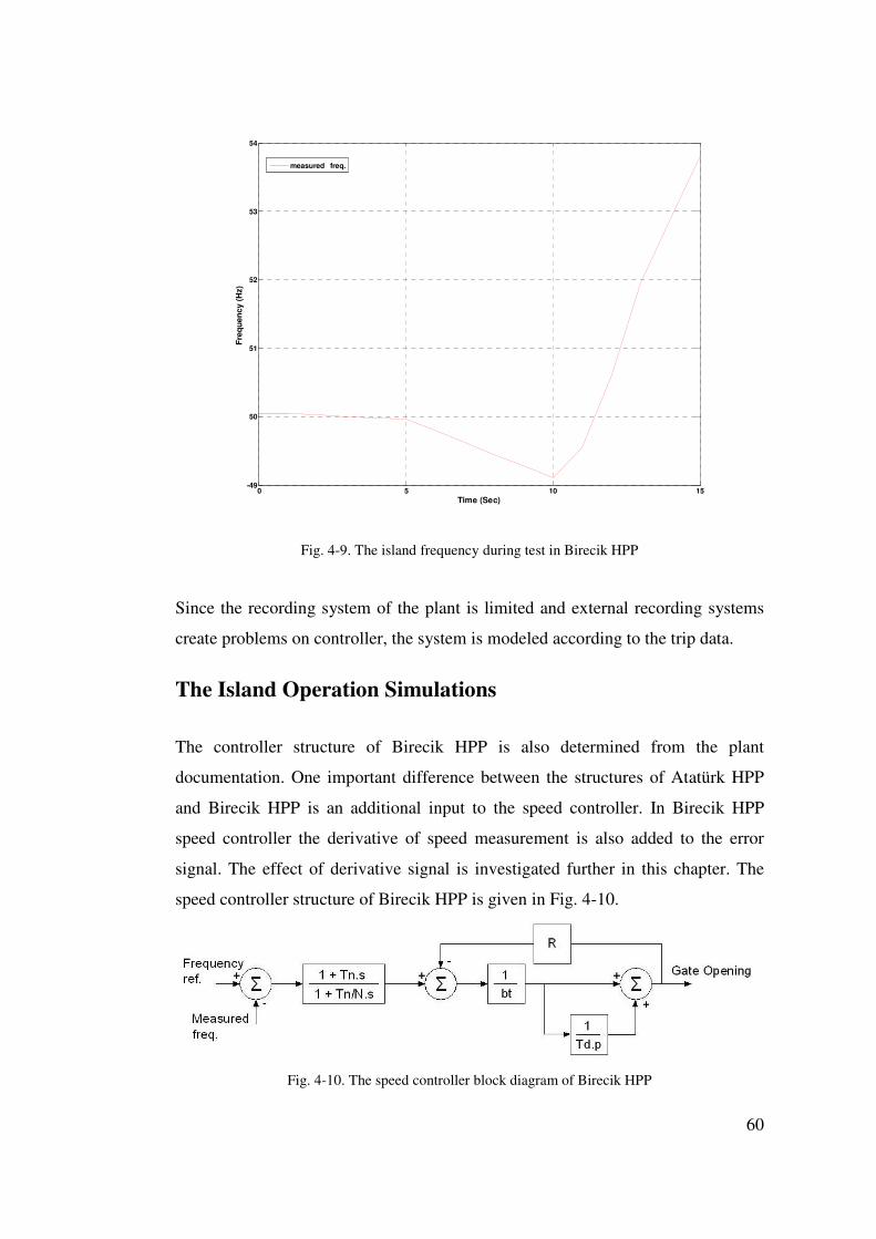
60
0 5 10 15-49
50
51
52
53
54
Time (Sec)
Fre
qu
ency
(H
z)
measured freq.
Fig. 4-9. The island frequency during test in Birecik HPP
Since the recording system of the plant is limited and external recording systems
create problems on controller, the system is modeled according to the trip data.
The Island Operation Simulations
The controller structure of Birecik HPP is also determined from the plant
documentation. One important difference between the structures of Atatürk HPP
and Birecik HPP is an additional input to the speed controller. In Birecik HPP
speed controller the derivative of speed measurement is also added to the error
signal. The effect of derivative signal is investigated further in this chapter. The
speed controller structure of Birecik HPP is given in Fig. 4-10.
Fig. 4-10. The speed controller block diagram of Birecik HPP
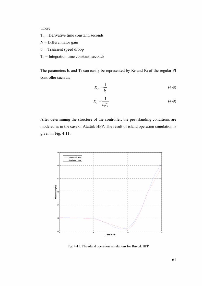
61
where
Tn = Derivative time constant, seconds
N = Differentiator gain
bt = Transient speed droop
Td = Integration time constant, seconds
The parameters bt and Td can easily be represented by KP and KI of the regular PI
controller such as;
t
Pb
K1
= (4-8)
dt
ITb
K1
= (4-9)
After determining the structure of the controller, the pre-islanding conditions are
modeled as in the case of Atatürk HPP. The result of island operation simulation is
given in Fig. 4-11.
0 5 10 1549
50
51
52
53
54
55
Time (Sec)
Fre
qu
ency
(H
z)
measured freq.
simulated freq.
Fig. 4-11. The island operation simulations for Birecik HPP
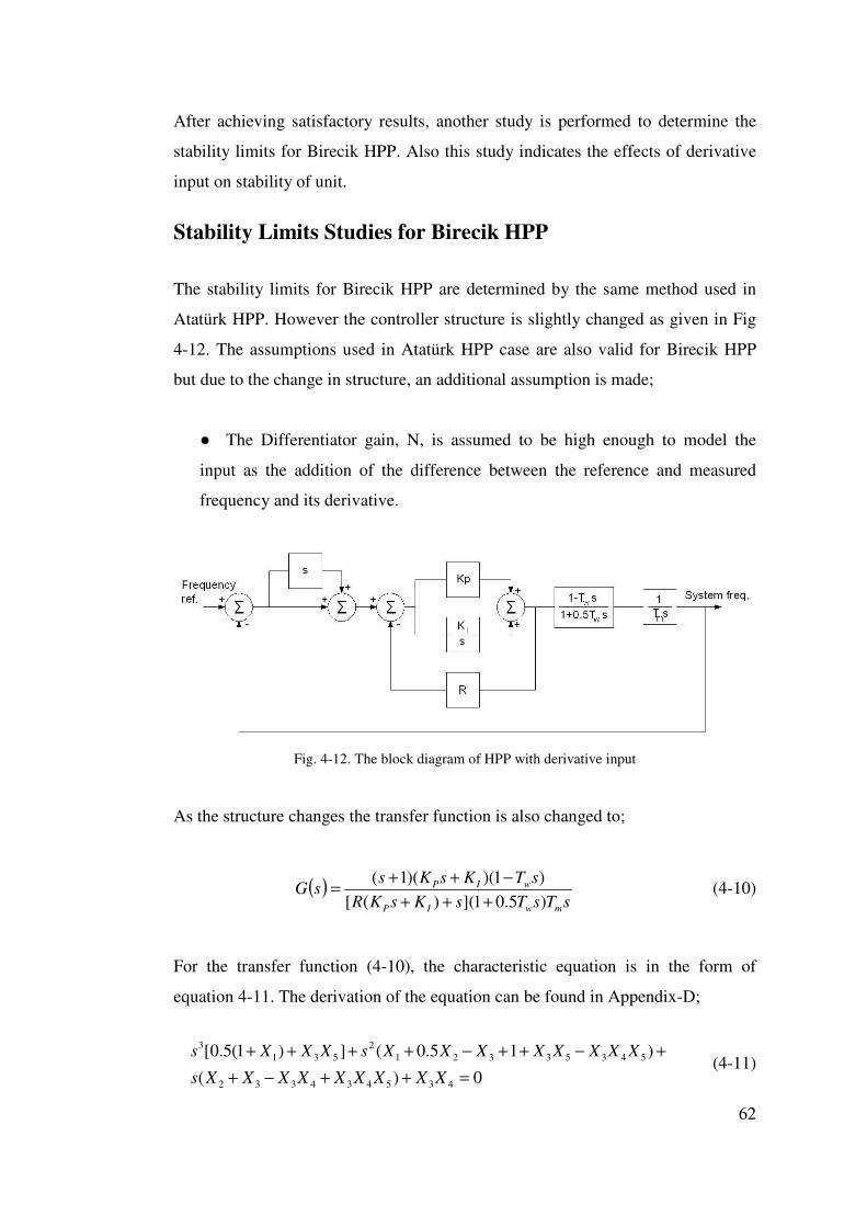
62
After achieving satisfactory results, another study is performed to determine the
stability limits for Birecik HPP. Also this study indicates the effects of derivative
input on stability of unit.
Stability Limits Studies for Birecik HPP
The stability limits for Birecik HPP are determined by the same method used in
Atatürk HPP. However the controller structure is slightly changed as given in Fig
4-12. The assumptions used in Atatürk HPP case are also valid for Birecik HPP
but due to the change in structure, an additional assumption is made;
● The Differentiator gain, N, is assumed to be high enough to model the
input as the addition of the difference between the reference and measured
frequency and its derivative.
Fig. 4-12. The block diagram of HPP with derivative input
As the structure changes the transfer function is also changed to;
( )sTsTsKsKR
sTKsKssG
mwIP
wIP
)5.01]()([
)1)()(1(
+++
−++= (4-10)
For the transfer function (4-10), the characteristic equation is in the form of
equation 4-11. The derivation of the equation can be found in Appendix-D;
0)(
)15.0(])1(5.0[
435434332
543533212
5313
=++−+
+−++−++++
XXXXXXXXXs
XXXXXXXXsXXXs (4-11)
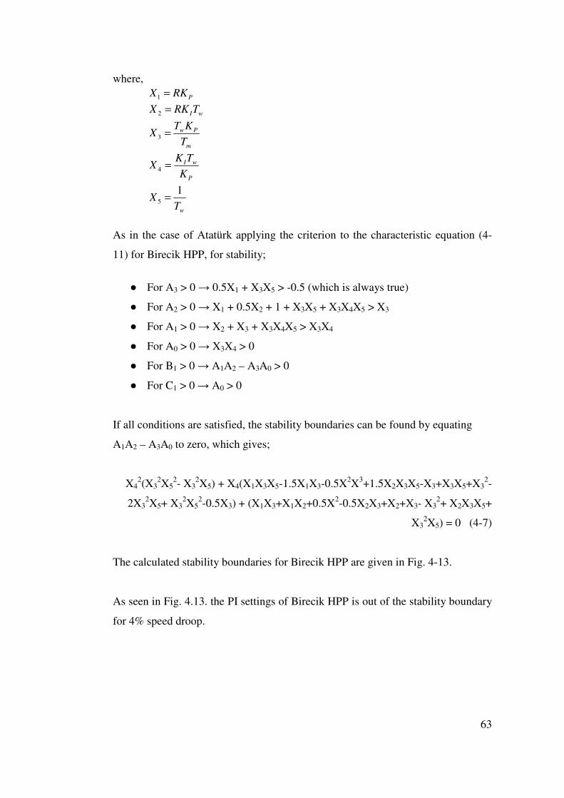
63
where,
PRKX =1
wITRKX =2
m
Pw
T
KTX =3
P
wI
K
TKX =4
wTX
15 =
As in the case of Atatürk applying the criterion to the characteristic equation (4-
11) for Birecik HPP, for stability;
● For A3 > 0 → 0.5X1 + X3X5 > -0.5 (which is always true)
● For A2 > 0 → X1 + 0.5X2 + 1 + X3X5 + X3X4X5 > X3
● For A1 > 0 → X2 + X3 + X3X4X5 > X3X4
● For A0 > 0 → X3X4 > 0
● For B1 > 0 → A1A2 – A3A0 > 0
● For C1 > 0 → A0 > 0
If all conditions are satisfied, the stability boundaries can be found by equating
A1A2 – A3A0 to zero, which gives;
X42(X3
2X52- X3
2X5) + X4(X1X3X5-1.5X1X3-0.5X2X3+1.5X2X3X5-X3+X3X5+X32-
2X32X5+ X3
2X52-0.5X3) + (X1X3+X1X2+0.5X2-0.5X2X3+X2+X3- X3
2+ X2X3X5+
X32X5) = 0 (4-7)
The calculated stability boundaries for Birecik HPP are given in Fig. 4-13.
As seen in Fig. 4.13. the PI settings of Birecik HPP is out of the stability boundary
for 4% speed droop.
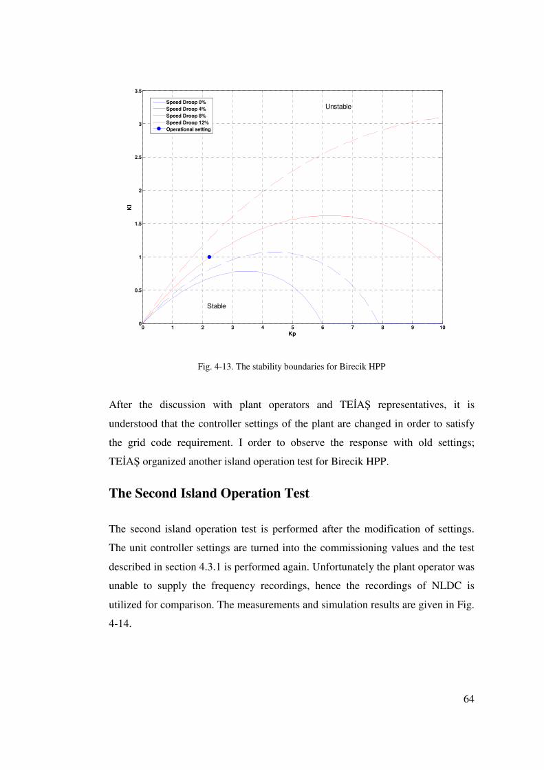
64
0 1 2 3 4 5 6 7 8 9 100
0.5
1
1.5
2
2.5
3
3.5
Kp
KI
Speed Droop 0%Speed Droop 4%Speed Droop 8%Speed Droop 12%Operational setting
Unstable
Stable
Fig. 4-13. The stability boundaries for Birecik HPP
After the discussion with plant operators and TEİAŞ representatives, it is
understood that the controller settings of the plant are changed in order to satisfy
the grid code requirement. I order to observe the response with old settings;
TEİAŞ organized another island operation test for Birecik HPP.
The Second Island Operation Test
The second island operation test is performed after the modification of settings.
The unit controller settings are turned into the commissioning values and the test
described in section 4.3.1 is performed again. Unfortunately the plant operator was
unable to supply the frequency recordings, hence the recordings of NLDC is
utilized for comparison. The measurements and simulation results are given in Fig.
4-14.
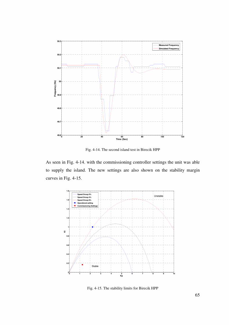
65
0 20 40 60 80 100 12049.6
49.7
49.8
49.9
50
50.1
50.2
50.3
Time (Sec)
Fre
qu
ency
(H
z)
Measured Frequency
Simulated Frequency
Fig. 4-14. The second island test in Birecik HPP
As seen in Fig. 4-14. with the commissioning controller settings the unit was able
to supply the island. The new settings are also shown on the stability margin
curves in Fig. 4-15.
0 1 2 3 4 5 6 7 8 9 100
0.2
0.4
0.6
0.8
1
1.2
1.4
1.6
1.8
Kp
KI
Speed Droop 0%
Speed Droop 4%
Speed Droop 8%
Operational setting
Commissioning Settings
Unstable
Stable
Fig. 4-15. The stability limits for Birecik HPP
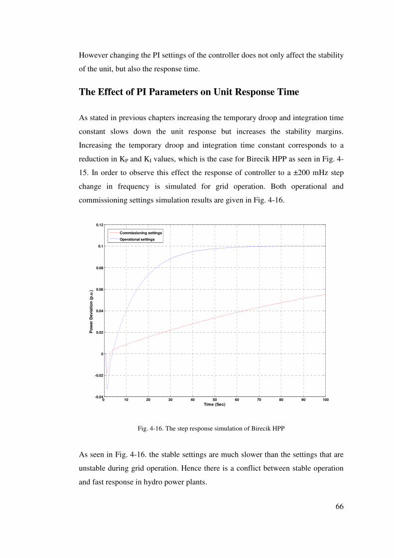
66
However changing the PI settings of the controller does not only affect the stability
of the unit, but also the response time.
The Effect of PI Parameters on Unit Response Time
As stated in previous chapters increasing the temporary droop and integration time
constant slows down the unit response but increases the stability margins.
Increasing the temporary droop and integration time constant corresponds to a
reduction in KP and KI values, which is the case for Birecik HPP as seen in Fig. 4-
15. In order to observe this effect the response of controller to a ±200 mHz step
change in frequency is simulated for grid operation. Both operational and
commissioning settings simulation results are given in Fig. 4-16.
0 10 20 30 40 50 60 70 80 90 100-0.04
-0.02
0
0.02
0.04
0.06
0.08
0.1
0.12
Time (Sec)
Po
wer
Dev
iati
on
(p
.u.)
Commissioning settings
Operational settings
Fig. 4-16. The step response simulation of Birecik HPP
As seen in Fig. 4-16. the stable settings are much slower than the settings that are
unstable during grid operation. Hence there is a conflict between stable operation
and fast response in hydro power plants.
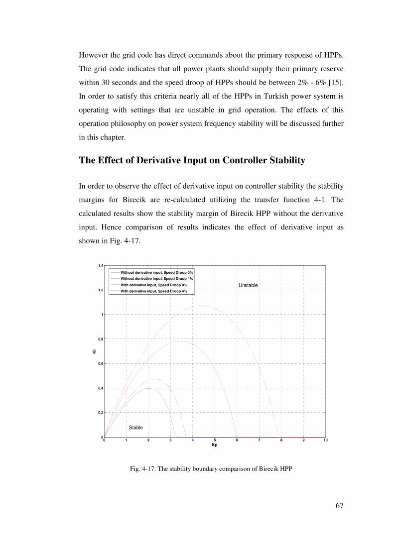
67
However the grid code has direct commands about the primary response of HPPs.
The grid code indicates that all power plants should supply their primary reserve
within 30 seconds and the speed droop of HPPs should be between 2% - 6% [15].
In order to satisfy this criteria nearly all of the HPPs in Turkish power system is
operating with settings that are unstable in grid operation. The effects of this
operation philosophy on power system frequency stability will be discussed further
in this chapter.
The Effect of Derivative Input on Controller Stability
In order to observe the effect of derivative input on controller stability the stability
margins for Birecik are re-calculated utilizing the transfer function 4-1. The
calculated results show the stability margin of Birecik HPP without the derivative
input. Hence comparison of results indicates the effect of derivative input as
shown in Fig. 4-17.
0 1 2 3 4 5 6 7 8 9 100
0.2
0.4
0.6
0.8
1
1.2
1.4
Kp
KI
Without derivative input, Speed Droop 0%
Without derivative input, Speed Droop 4%
With derivative input, Speed Droop 0%
With derivative input, Speed Droop 4%
Unstable
Stable
Fig. 4-17. The stability boundary comparison of Birecik HPP
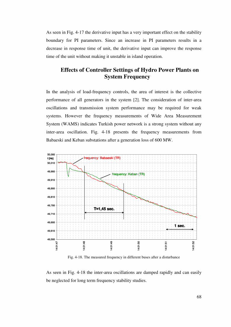
68
As seen in Fig. 4-17 the derivative input has a very important effect on the stability
boundary for PI parameters. Since an increase in PI parameters results in a
decrease in response time of unit, the derivative input can improve the response
time of the unit without making it unstable in island operation.
4.4. Effects of Controller Settings of Hydro Power Plants on System Frequency
In the analysis of load-frequency controls, the area of interest is the collective
performance of all generators in the system [2]. The consideration of inter-area
oscillations and transmission system performance may be required for weak
systems. However the frequency measurements of Wide Area Measurement
System (WAMS) indicates Turkish power network is a strong system without any
inter-area oscillation. Fig. 4-18 presents the frequency measurements from
Babaeski and Keban substations after a generation loss of 600 MW.
49,560
49,610
49,660
49,710
49,760
49,810
49,860
49,910
49,960
50,010
50,060
14:
01:
47
14:
01:
48
14:
01:
49
14:
01:
50
14:
01:
51
14:
01:
52
f [Hz] frequency: Babaeski (TR)
frequency: Keban (TR)
1 sec.
T≈1,45 sec.
49,560
49,610
49,660
49,710
49,760
49,810
49,860
49,910
49,960
50,010
50,060
14:
01:
47
14:
01:
48
14:
01:
49
14:
01:
50
14:
01:
51
14:
01:
52
f [Hz] frequency: Babaeski (TR)
frequency: Keban (TR)
1 sec.1 sec.
T≈1,45 sec.T≈1,45 sec.
Fig. 4-18. The measured frequency in different buses after a disturbance
As seen in Fig. 4-18 the inter-area oscillations are damped rapidly and can easily
be neglected for long term frequency stability studies.
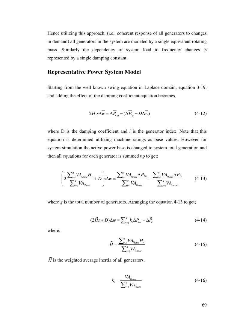
69
Hence utilizing this approach, (i.e., coherent response of all generators to changes
in demand) all generators in the system are modeled by a single equivalent rotating
mass. Similarly the dependency of system load to frequency changes is
represented by a single damping constant.
Representative Power System Model
Starting from the well known swing equation in Laplace domain, equation 3-19,
and adding the effect of the damping coefficient equation becomes,
)(2 wDPPwsHeimii ∆−∆−∆=∆ (4-12)
where D is the damping coefficient and i is the generator index. Note that this
equation is determined utilizing machine ratings as base values. However for
system simulation the active power base is changed to system total generation and
then all equations for each generator is summed up to get;
∑∑
∑∑
∑∑
=
=
=
=
=
=∆
−∆
=∆
+
g
i basei
g
iei
basei
g
i basei
g
imi
basei
g
i basei
g
i ibasei
VA
PVA
VA
PVAwsD
VA
HVA
1
1
1
1
1
12 (4-13)
where g is the total number of generators. Arranging the equation 4-13 to get;
e
g
i mii PPkwDsH~
)~
2(1
∆−∆=∆+ ∑ = (4-14)
where;
∑∑
=
==g
i basei
g
i ibasei
VA
HVAH
1
1~ (4-15)
H~
is the weighted average inertia of all generators.
∑ =
=g
i basei
basei
i
VA
VAk
1
(4-16)
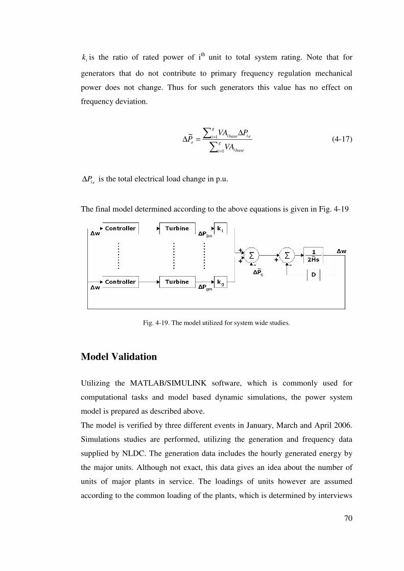
70
ik is the ratio of rated power of ith unit to total system rating. Note that for
generators that do not contribute to primary frequency regulation mechanical
power does not change. Thus for such generators this value has no effect on
frequency deviation.
∑∑
=
=∆
=∆g
i basei
ei
g
i basei
e
VA
PVAP
1
1~ (4-17)
eiP∆ is the total electrical load change in p.u.
The final model determined according to the above equations is given in Fig. 4-19
Fig. 4-19. The model utilized for system wide studies.
Model Validation
Utilizing the MATLAB/SIMULINK software, which is commonly used for
computational tasks and model based dynamic simulations, the power system
model is prepared as described above.
The model is verified by three different events in January, March and April 2006.
Simulations studies are performed, utilizing the generation and frequency data
supplied by NLDC. The generation data includes the hourly generated energy by
the major units. Although not exact, this data gives an idea about the number of
units of major plants in service. The loadings of units however are assumed
according to the common loading of the plants, which is determined by interviews
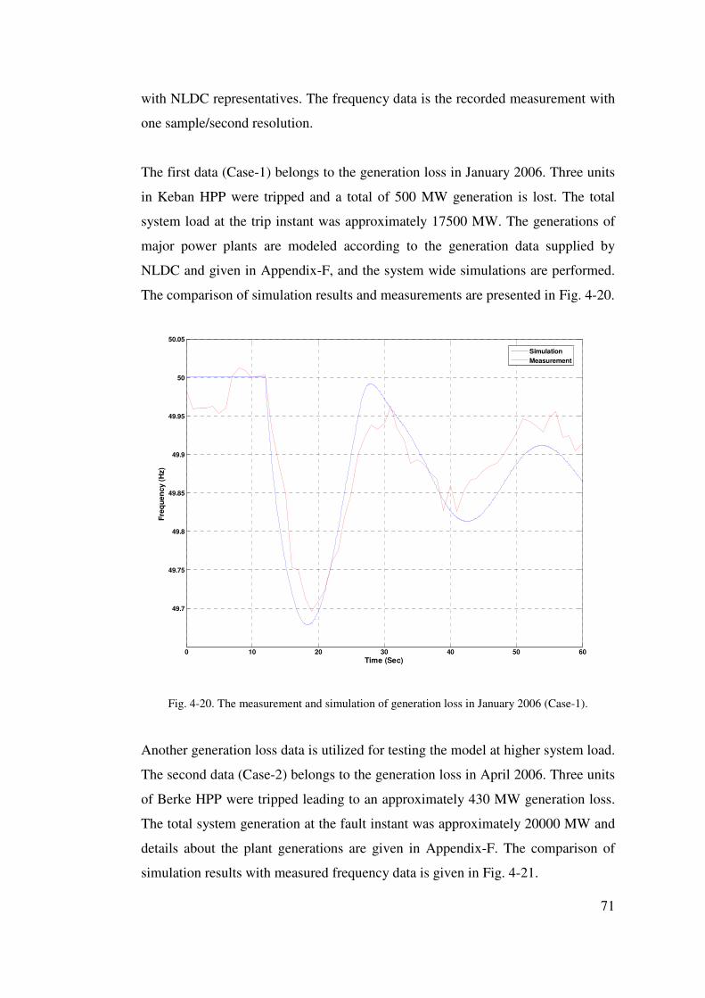
71
with NLDC representatives. The frequency data is the recorded measurement with
one sample/second resolution.
The first data (Case-1) belongs to the generation loss in January 2006. Three units
in Keban HPP were tripped and a total of 500 MW generation is lost. The total
system load at the trip instant was approximately 17500 MW. The generations of
major power plants are modeled according to the generation data supplied by
NLDC and given in Appendix-F, and the system wide simulations are performed.
The comparison of simulation results and measurements are presented in Fig. 4-20.
0 10 20 30 40 50 60
49.7
49.75
49.8
49.85
49.9
49.95
50
50.05
Time (Sec)
Fre
qu
ency
(H
z)
Simulation
Measurement
Fig. 4-20. The measurement and simulation of generation loss in January 2006 (Case-1).
Another generation loss data is utilized for testing the model at higher system load.
The second data (Case-2) belongs to the generation loss in April 2006. Three units
of Berke HPP were tripped leading to an approximately 430 MW generation loss.
The total system generation at the fault instant was approximately 20000 MW and
details about the plant generations are given in Appendix-F. The comparison of
simulation results with measured frequency data is given in Fig. 4-21.
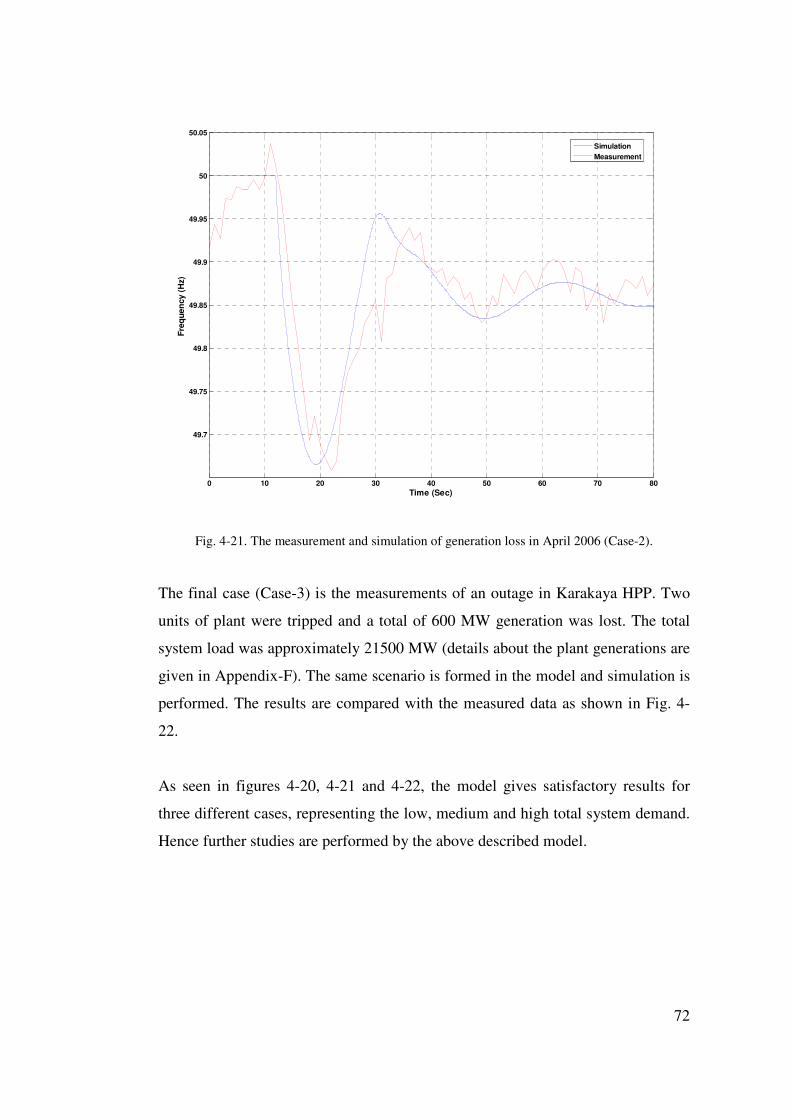
72
0 10 20 30 40 50 60 70 80
49.7
49.75
49.8
49.85
49.9
49.95
50
50.05
Time (Sec)
Fre
qu
ency
(H
z)
Simulation
Measurement
Fig. 4-21. The measurement and simulation of generation loss in April 2006 (Case-2).
The final case (Case-3) is the measurements of an outage in Karakaya HPP. Two
units of plant were tripped and a total of 600 MW generation was lost. The total
system load was approximately 21500 MW (details about the plant generations are
given in Appendix-F). The same scenario is formed in the model and simulation is
performed. The results are compared with the measured data as shown in Fig. 4-
22.
As seen in figures 4-20, 4-21 and 4-22, the model gives satisfactory results for
three different cases, representing the low, medium and high total system demand.
Hence further studies are performed by the above described model.
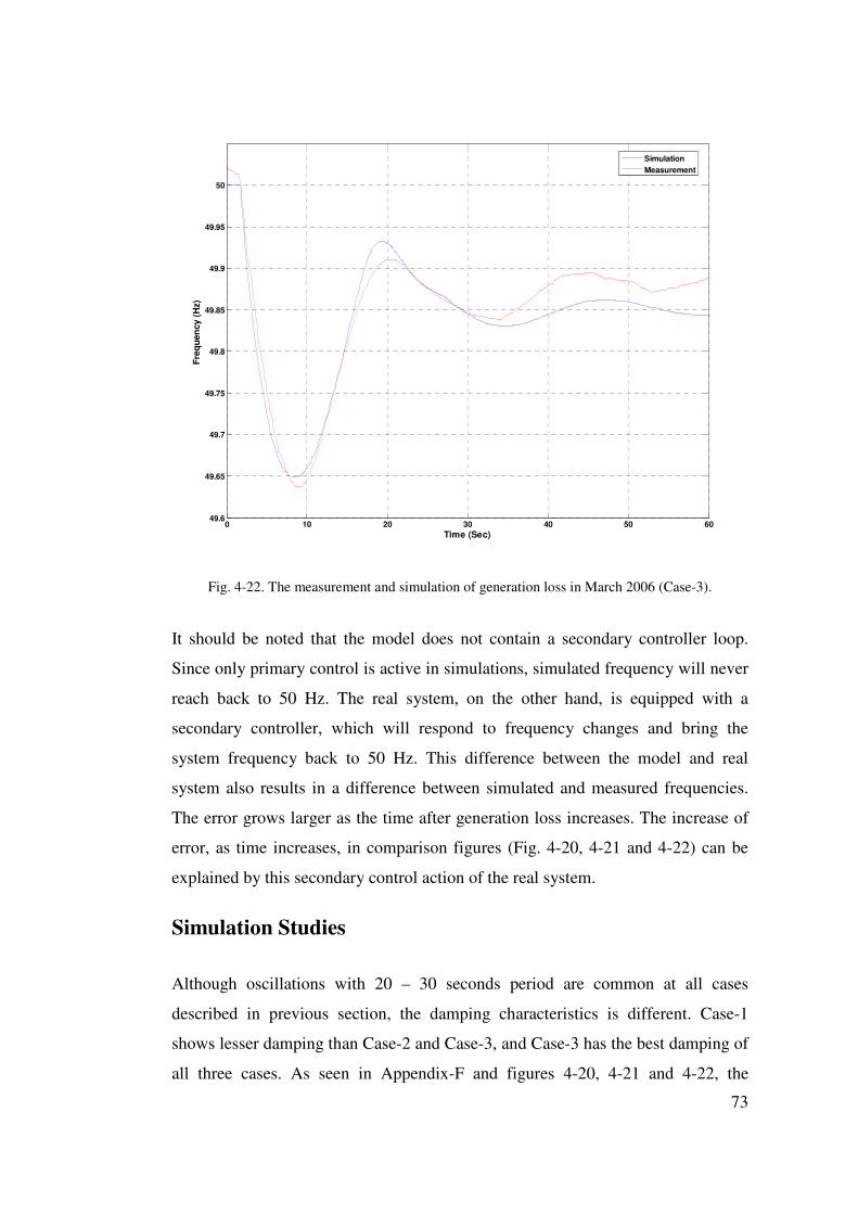
73
0 10 20 30 40 50 6049.6
49.65
49.7
49.75
49.8
49.85
49.9
49.95
50
Time (Sec)
Fre
qu
ency
(H
z)
Simulation
Measurement
Fig. 4-22. The measurement and simulation of generation loss in March 2006 (Case-3).
It should be noted that the model does not contain a secondary controller loop.
Since only primary control is active in simulations, simulated frequency will never
reach back to 50 Hz. The real system, on the other hand, is equipped with a
secondary controller, which will respond to frequency changes and bring the
system frequency back to 50 Hz. This difference between the model and real
system also results in a difference between simulated and measured frequencies.
The error grows larger as the time after generation loss increases. The increase of
error, as time increases, in comparison figures (Fig. 4-20, 4-21 and 4-22) can be
explained by this secondary control action of the real system.
Simulation Studies
Although oscillations with 20 – 30 seconds period are common at all cases
described in previous section, the damping characteristics is different. Case-1
shows lesser damping than Case-2 and Case-3, and Case-3 has the best damping of
all three cases. As seen in Appendix-F and figures 4-20, 4-21 and 4-22, the
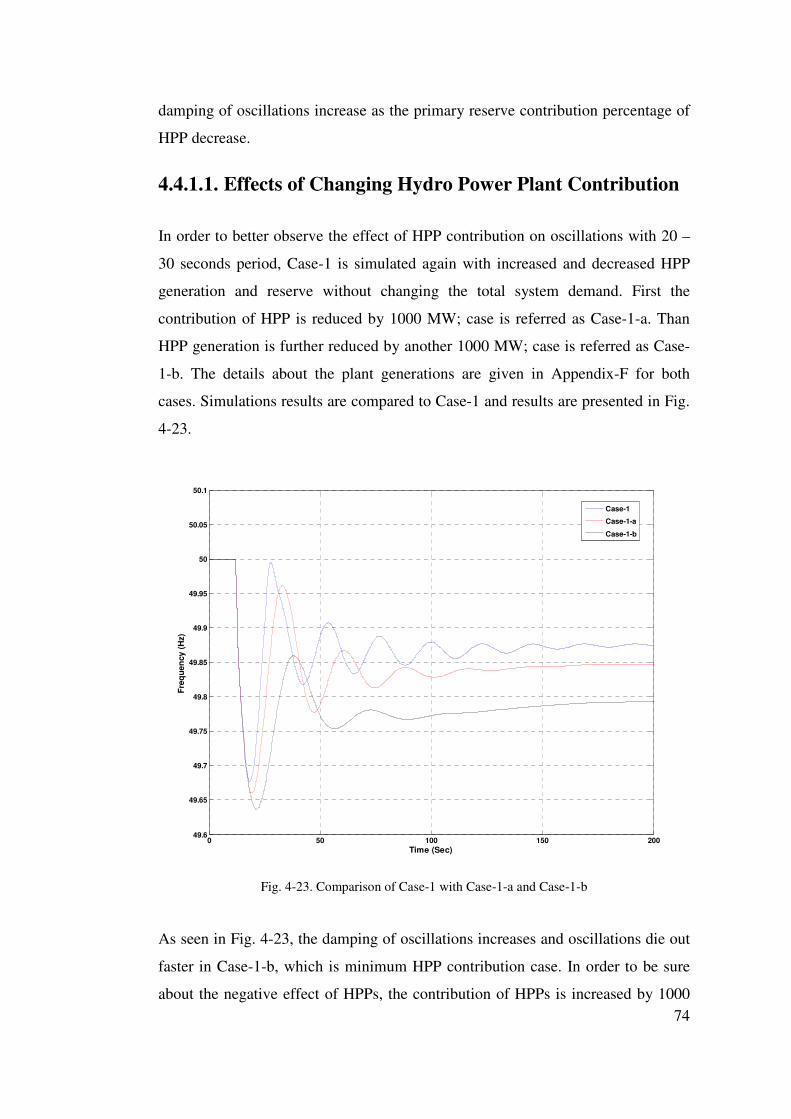
74
damping of oscillations increase as the primary reserve contribution percentage of
HPP decrease.
4.4.1.1. Effects of Changing Hydro Power Plant Contribution
In order to better observe the effect of HPP contribution on oscillations with 20 –
30 seconds period, Case-1 is simulated again with increased and decreased HPP
generation and reserve without changing the total system demand. First the
contribution of HPP is reduced by 1000 MW; case is referred as Case-1-a. Than
HPP generation is further reduced by another 1000 MW; case is referred as Case-
1-b. The details about the plant generations are given in Appendix-F for both
cases. Simulations results are compared to Case-1 and results are presented in Fig.
4-23.
0 50 100 150 20049.6
49.65
49.7
49.75
49.8
49.85
49.9
49.95
50
50.05
50.1
Time (Sec)
Fre
qu
ency
(H
z)
Case-1
Case-1-a
Case-1-b
Fig. 4-23. Comparison of Case-1 with Case-1-a and Case-1-b
As seen in Fig. 4-23, the damping of oscillations increases and oscillations die out
faster in Case-1-b, which is minimum HPP contribution case. In order to be sure
about the negative effect of HPPs, the contribution of HPPs is increased by 1000
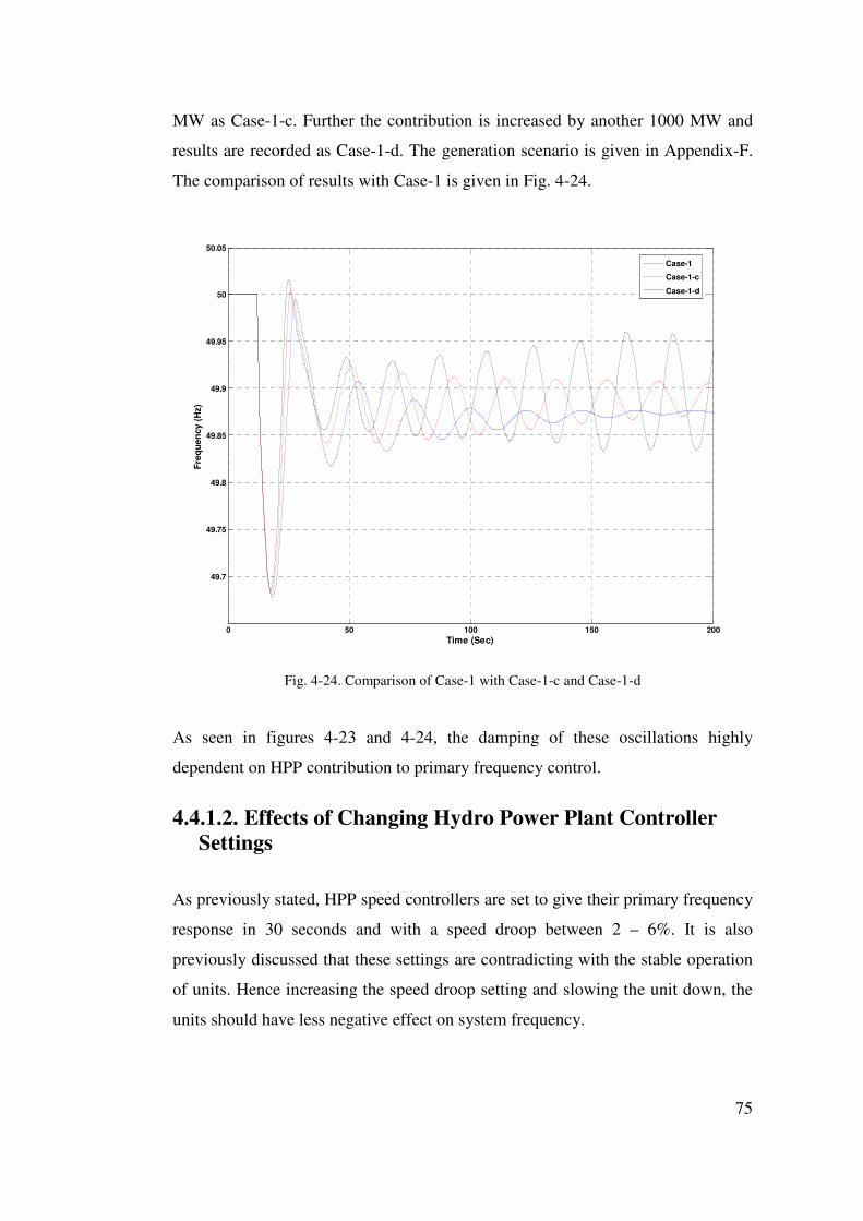
75
MW as Case-1-c. Further the contribution is increased by another 1000 MW and
results are recorded as Case-1-d. The generation scenario is given in Appendix-F.
The comparison of results with Case-1 is given in Fig. 4-24.
0 50 100 150 200
49.7
49.75
49.8
49.85
49.9
49.95
50
50.05
Time (Sec)
Fre
qu
ency
(H
z)
Case-1
Case-1-c
Case-1-d
Fig. 4-24. Comparison of Case-1 with Case-1-c and Case-1-d
As seen in figures 4-23 and 4-24, the damping of these oscillations highly
dependent on HPP contribution to primary frequency control.
4.4.1.2. Effects of Changing Hydro Power Plant Controller Settings
As previously stated, HPP speed controllers are set to give their primary frequency
response in 30 seconds and with a speed droop between 2 – 6%. It is also
previously discussed that these settings are contradicting with the stable operation
of units. Hence increasing the speed droop setting and slowing the unit down, the
units should have less negative effect on system frequency.
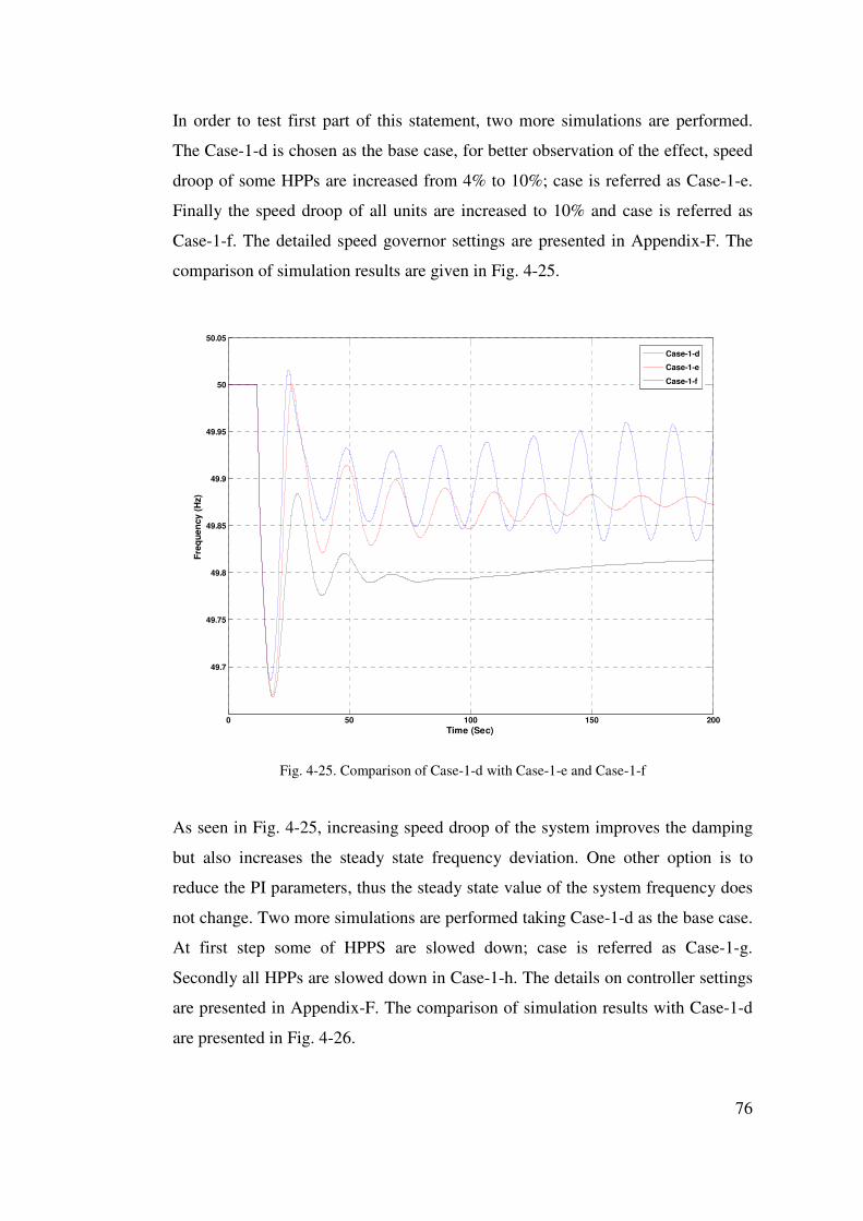
76
In order to test first part of this statement, two more simulations are performed.
The Case-1-d is chosen as the base case, for better observation of the effect, speed
droop of some HPPs are increased from 4% to 10%; case is referred as Case-1-e.
Finally the speed droop of all units are increased to 10% and case is referred as
Case-1-f. The detailed speed governor settings are presented in Appendix-F. The
comparison of simulation results are given in Fig. 4-25.
0 50 100 150 200
49.7
49.75
49.8
49.85
49.9
49.95
50
50.05
Time (Sec)
Fre
qu
ency
(H
z)
Case-1-d
Case-1-e
Case-1-f
Fig. 4-25. Comparison of Case-1-d with Case-1-e and Case-1-f
As seen in Fig. 4-25, increasing speed droop of the system improves the damping
but also increases the steady state frequency deviation. One other option is to
reduce the PI parameters, thus the steady state value of the system frequency does
not change. Two more simulations are performed taking Case-1-d as the base case.
At first step some of HPPS are slowed down; case is referred as Case-1-g.
Secondly all HPPs are slowed down in Case-1-h. The details on controller settings
are presented in Appendix-F. The comparison of simulation results with Case-1-d
are presented in Fig. 4-26.
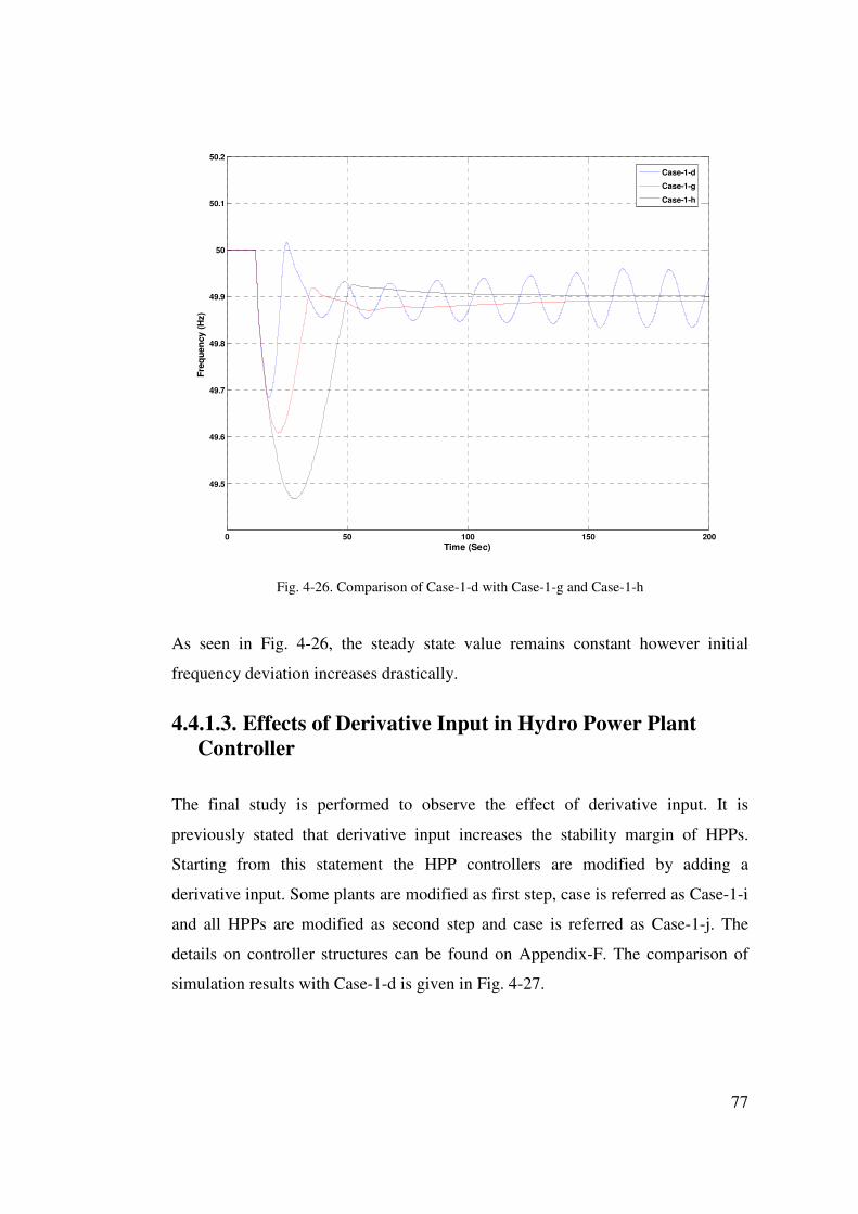
77
0 50 100 150 200
49.5
49.6
49.7
49.8
49.9
50
50.1
50.2
Time (Sec)
Fre
qu
ency
(H
z)
Case-1-d
Case-1-g
Case-1-h
Fig. 4-26. Comparison of Case-1-d with Case-1-g and Case-1-h
As seen in Fig. 4-26, the steady state value remains constant however initial
frequency deviation increases drastically.
4.4.1.3. Effects of Derivative Input in Hydro Power Plant Controller
The final study is performed to observe the effect of derivative input. It is
previously stated that derivative input increases the stability margin of HPPs.
Starting from this statement the HPP controllers are modified by adding a
derivative input. Some plants are modified as first step, case is referred as Case-1-i
and all HPPs are modified as second step and case is referred as Case-1-j. The
details on controller structures can be found on Appendix-F. The comparison of
simulation results with Case-1-d is given in Fig. 4-27.
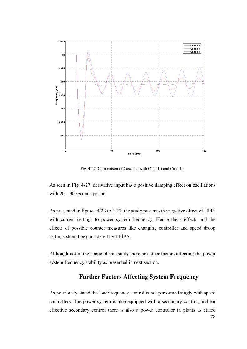
78
0 50 100 150
49.7
49.75
49.8
49.85
49.9
49.95
50
50.05
Time (Sec)
Fre
qu
ency
(H
z)
Case-1-dCase-1-iCase-1-j
Fig. 4-27. Comparison of Case-1-d with Case-1-i and Case-1-j
As seen in Fig. 4-27, derivative input has a positive damping effect on oscillations
with 20 – 30 seconds period.
As presented in figures 4-23 to 4-27, the study presents the negative effect of HPPs
with current settings to power system frequency. Hence these effects and the
effects of possible counter measures like changing controller and speed droop
settings should be considered by TEİAŞ.
Although not in the scope of this study there are other factors affecting the power
system frequency stability as presented in next section.
4.5. Further Factors Affecting System Frequency
As previously stated the load/frequency control is not performed singly with speed
controllers. The power system is also equipped with a secondary control, and for
effective secondary control there is also a power controller in plants as stated
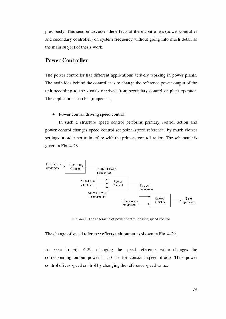
79
previously. This section discusses the effects of these controllers (power controller
and secondary controller) on system frequency without going into much detail as
the main subject of thesis work.
Power Controller
The power controller has different applications actively working in power plants.
The main idea behind the controller is to change the reference power output of the
unit according to the signals received from secondary control or plant operator.
The applications can be grouped as;
● Power control driving speed control;
In such a structure speed control performs primary control action and
power control changes speed control set point (speed reference) by much slower
settings in order not to interfere with the primary control action. The schematic is
given in Fig. 4-28.
Fig. 4-28. The schematic of power control driving speed control
The change of speed reference effects unit output as shown in Fig. 4-29.
As seen in Fig. 4-29, changing the speed reference value changes the
corresponding output power at 50 Hz for constant speed droop. Thus power
control drives speed control by changing the reference speed value.
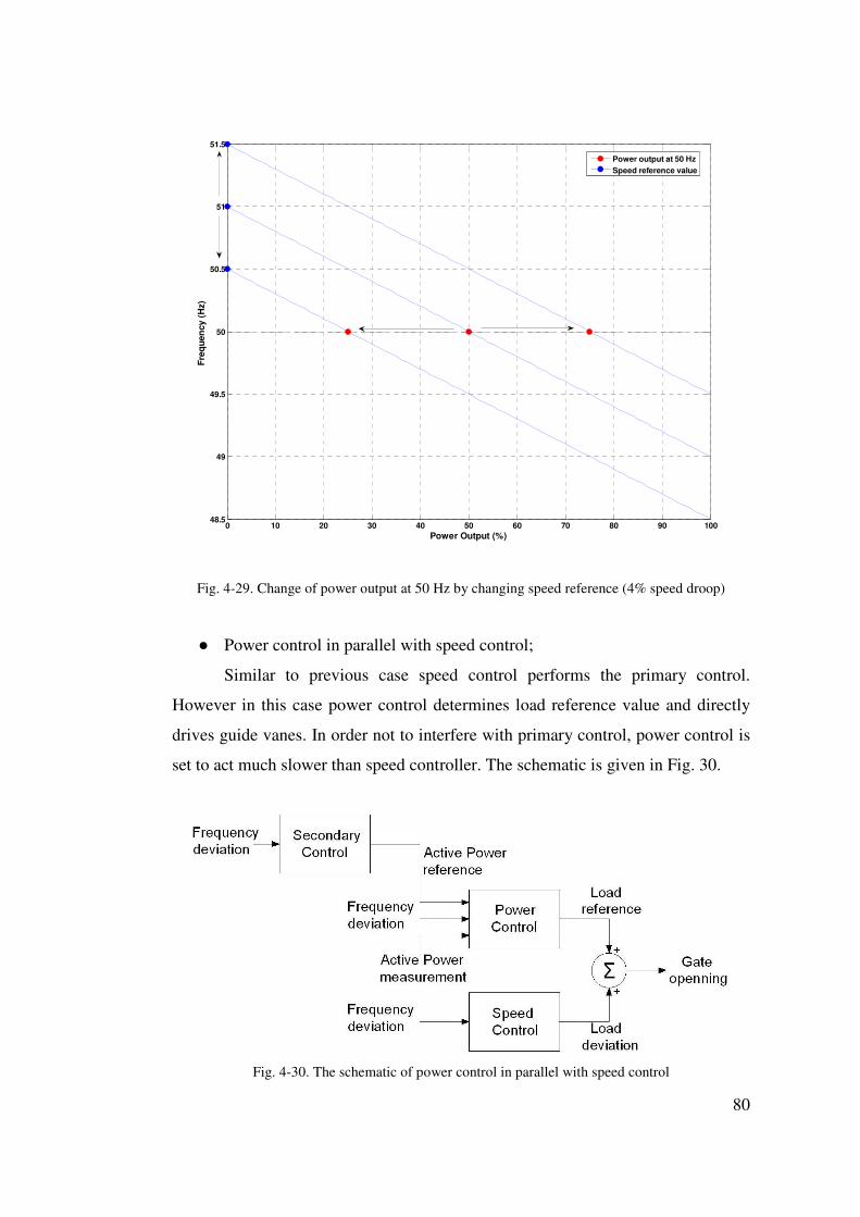
80
0 10 20 30 40 50 60 70 80 90 10048.5
49
49.5
50
50.5
51
51.5
Power Output (%)
Fre
qu
ency
(H
z)
Power output at 50 Hz
Speed reference value
Fig. 4-29. Change of power output at 50 Hz by changing speed reference (4% speed droop)
● Power control in parallel with speed control;
Similar to previous case speed control performs the primary control.
However in this case power control determines load reference value and directly
drives guide vanes. In order not to interfere with primary control, power control is
set to act much slower than speed controller. The schematic is given in Fig. 30.
Fig. 4-30. The schematic of power control in parallel with speed control
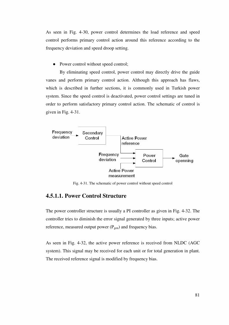
81
As seen in Fig. 4-30, power control determines the load reference and speed
control performs primary control action around this reference according to the
frequency deviation and speed droop setting.
● Power control without speed control;
By eliminating speed control, power control may directly drive the guide
vanes and perform primary control action. Although this approach has flaws,
which is described in further sections, it is commonly used in Turkish power
system. Since the speed control is deactivated, power control settings are tuned in
order to perform satisfactory primary control action. The schematic of control is
given in Fig. 4-31.
Fig. 4-31. The schematic of power control without speed control
4.5.1.1. Power Control Structure
The power controller structure is usually a PI controller as given in Fig. 4-32. The
controller tries to diminish the error signal generated by three inputs; active power
reference, measured output power (Pgen) and frequency bias.
As seen in Fig. 4-32, the active power reference is received from NLDC (AGC
system). This signal may be received for each unit or for total generation in plant.
The received reference signal is modified by frequency bias.
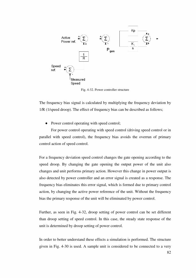
82
Fig. 4-32. Power controller structure
The frequency bias signal is calculated by multiplying the frequency deviation by
1/R (1/speed droop). The effect of frequency bias can be described as follows;
● Power control operating with speed control;
For power control operating with speed control (driving speed control or in
parallel with speed control), the frequency bias avoids the overrun of primary
control action of speed control.
For a frequency deviation speed control changes the gate opening according to the
speed droop. By changing the gate opening the output power of the unit also
changes and unit performs primary action. However this change in power output is
also detected by power controller and an error signal is created as a response. The
frequency bias eliminates this error signal, which is formed due to primary control
action, by changing the active power reference of the unit. Without the frequency
bias the primary response of the unit will be eliminated by power control.
Further, as seen in Fig. 4-32, droop setting of power control can be set different
than droop setting of speed control. In this case, the steady state response of the
unit is determined by droop setting of power control.
In order to better understand these effects a simulation is performed. The structure
given in Fig. 4-30 is used. A sample unit is considered to be connected to a very
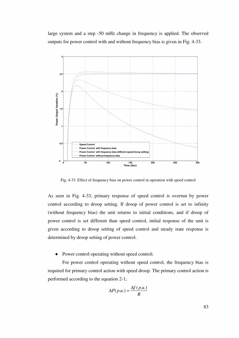
83
large system and a step -50 mHz change in frequency is applied. The observed
outputs for power control with and without frequency bias is given in Fig. 4-33.
0 50 100 150 200 250 3000
0.5
1
1.5
2
2.5
3
Time (Sec)
Po
wer
Ou
tpu
t V
aria
tio
n (
%)
Speed Control
Power Control with frequency bias
Power Control with frequency bias (different speed droop setting)
Power Control without frequency bias
Fig. 4-33. Effect of frequency bias on power control in operation with speed control
As seen in Fig. 4-33, primary response of speed control is overrun by power
control according to droop setting. If droop of power control is set to infinity
(without frequency bias) the unit returns to initial conditions, and if droop of
power control is set different than speed control, initial response of the unit is
given according to droop setting of speed control and steady state response is
determined by droop setting of power control.
● Power control operating without speed control;
For power control operating without speed control, the frequency bias is
required for primary control action with speed droop. The primary control action is
performed according to the equation 2-1;
R
upfupP
.).(.).(
∆=∆
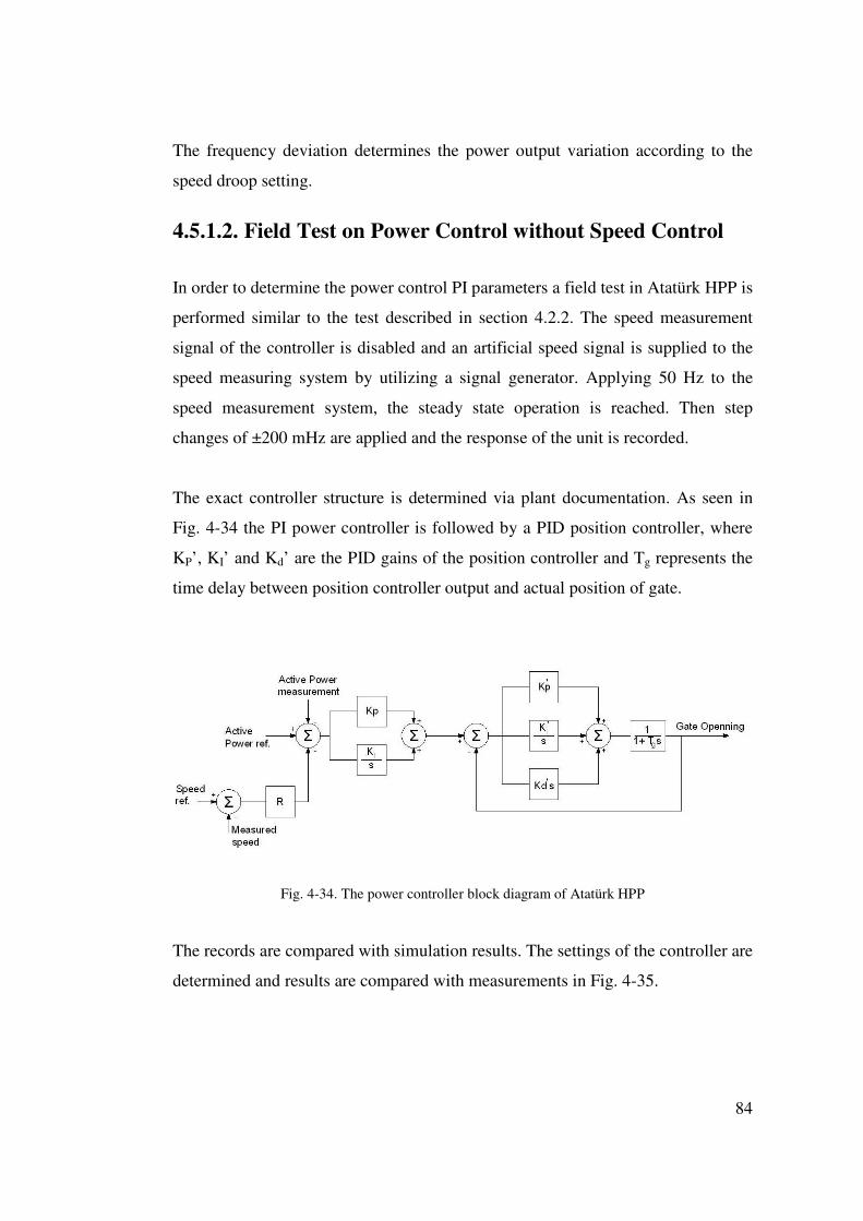
84
The frequency deviation determines the power output variation according to the
speed droop setting.
4.5.1.2. Field Test on Power Control without Speed Control
In order to determine the power control PI parameters a field test in Atatürk HPP is
performed similar to the test described in section 4.2.2. The speed measurement
signal of the controller is disabled and an artificial speed signal is supplied to the
speed measuring system by utilizing a signal generator. Applying 50 Hz to the
speed measurement system, the steady state operation is reached. Then step
changes of ±200 mHz are applied and the response of the unit is recorded.
The exact controller structure is determined via plant documentation. As seen in
Fig. 4-34 the PI power controller is followed by a PID position controller, where
KP’, KI’ and Kd’ are the PID gains of the position controller and Tg represents the
time delay between position controller output and actual position of gate.
Fig. 4-34. The power controller block diagram of Atatürk HPP
The records are compared with simulation results. The settings of the controller are
determined and results are compared with measurements in Fig. 4-35.
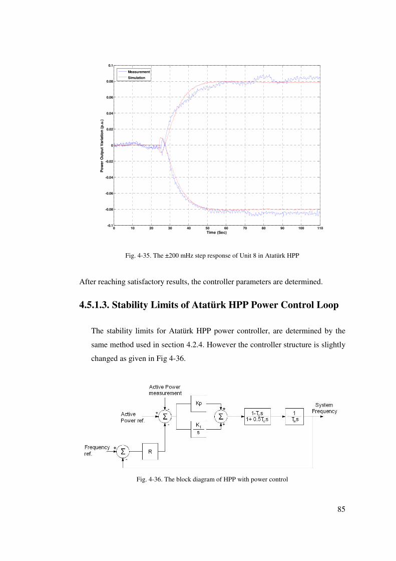
85
0 10 20 30 40 50 60 70 80 90 100 110-0.1
-0.08
-0.06
-0.04
-0.02
0
0.02
0.04
0.06
0.08
0.1
Time (Sec)
Po
wer
Ou
tpu
t V
aria
tio
n (
p.u
.)
Measurement
Simulation
Fig. 4-35. The ±200 mHz step response of Unit 8 in Atatürk HPP
After reaching satisfactory results, the controller parameters are determined.
4.5.1.3. Stability Limits of Atatürk HPP Power Control Loop
The stability limits for Atatürk HPP power controller, are determined by the
same method used in section 4.2.4. However the controller structure is slightly
changed as given in Fig 4-36.
Fig. 4-36. The block diagram of HPP with power control
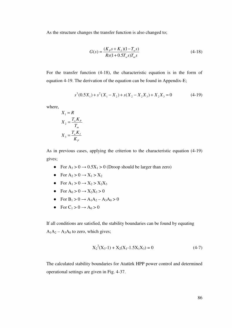
86
As the structure changes the transfer function is also changed to;
sTsTRs
sTKsKsG
mw
wIP
)5.01(
)1)(()(
+
−+= (4-18)
For the transfer function (4-18), the characteristic equation is in the form of
equation 4-19. The derivation of the equation can be found in Appendix-E;
0)()()5.0( 32322212
13 =+−+−+ XXXXXsXXsXs (4-19)
where,
RX =1
m
Pw
T
KTX =2
P
Iw
K
KTX =3
As in previous cases, applying the criterion to the characteristic equation (4-19)
gives;
● For A3 > 0 → 0.5X1 > 0 (Droop should be larger than zero)
● For A2 > 0 → X1 > X2
● For A1 > 0 → X2 > X2X3
● For A0 > 0 → X2X3 > 0
● For B1 > 0 → A1A2 – A3A0 > 0
● For C1 > 0 → A0 > 0
If all conditions are satisfied, the stability boundaries can be found by equating
A1A2 – A3A0 to zero, which gives;
X22(X3-1) + X2(X1-1.5X1X3) = 0 (4-7)
The calculated stability boundaries for Atatürk HPP power control and determined
operational settings are given in Fig. 4-37.
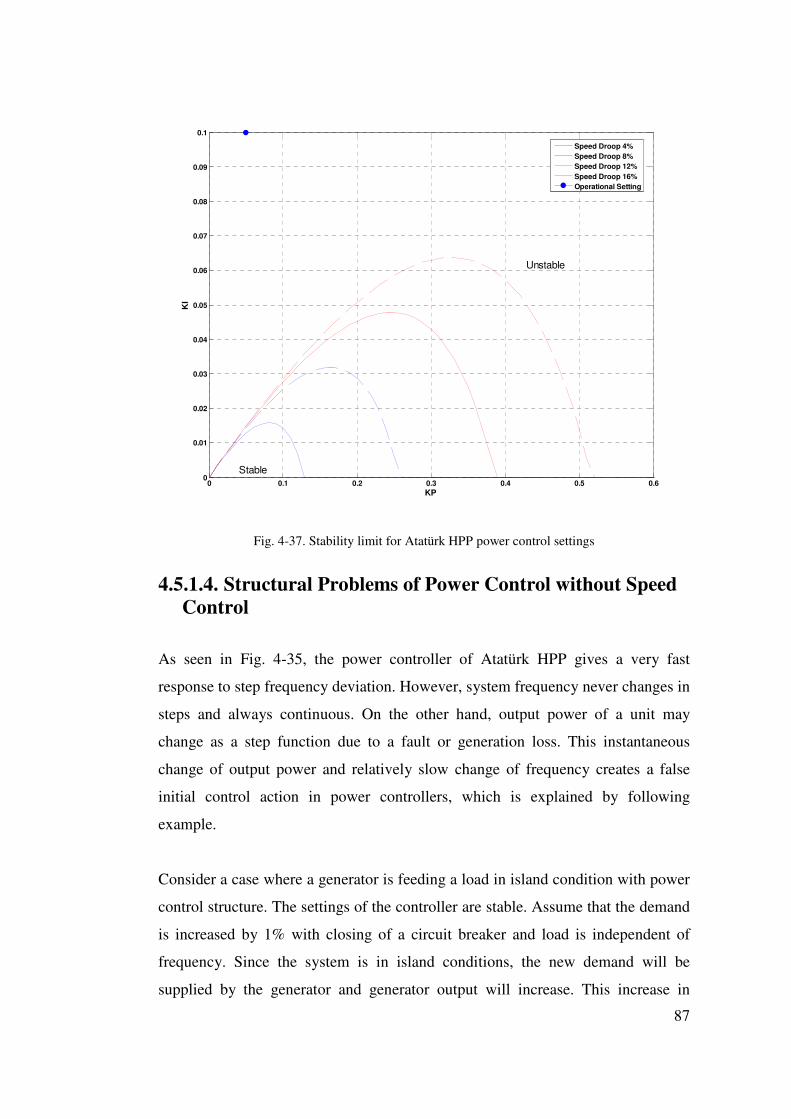
87
0 0.1 0.2 0.3 0.4 0.5 0.60
0.01
0.02
0.03
0.04
0.05
0.06
0.07
0.08
0.09
0.1
KP
KI
Speed Droop 4%Speed Droop 8%Speed Droop 12%Speed Droop 16%Operational Setting
Unstable
Stable
Fig. 4-37. Stability limit for Atatürk HPP power control settings
4.5.1.4. Structural Problems of Power Control without Speed Control
As seen in Fig. 4-35, the power controller of Atatürk HPP gives a very fast
response to step frequency deviation. However, system frequency never changes in
steps and always continuous. On the other hand, output power of a unit may
change as a step function due to a fault or generation loss. This instantaneous
change of output power and relatively slow change of frequency creates a false
initial control action in power controllers, which is explained by following
example.
Consider a case where a generator is feeding a load in island condition with power
control structure. The settings of the controller are stable. Assume that the demand
is increased by 1% with closing of a circuit breaker and load is independent of
frequency. Since the system is in island conditions, the new demand will be
supplied by the generator and generator output will increase. This increase in
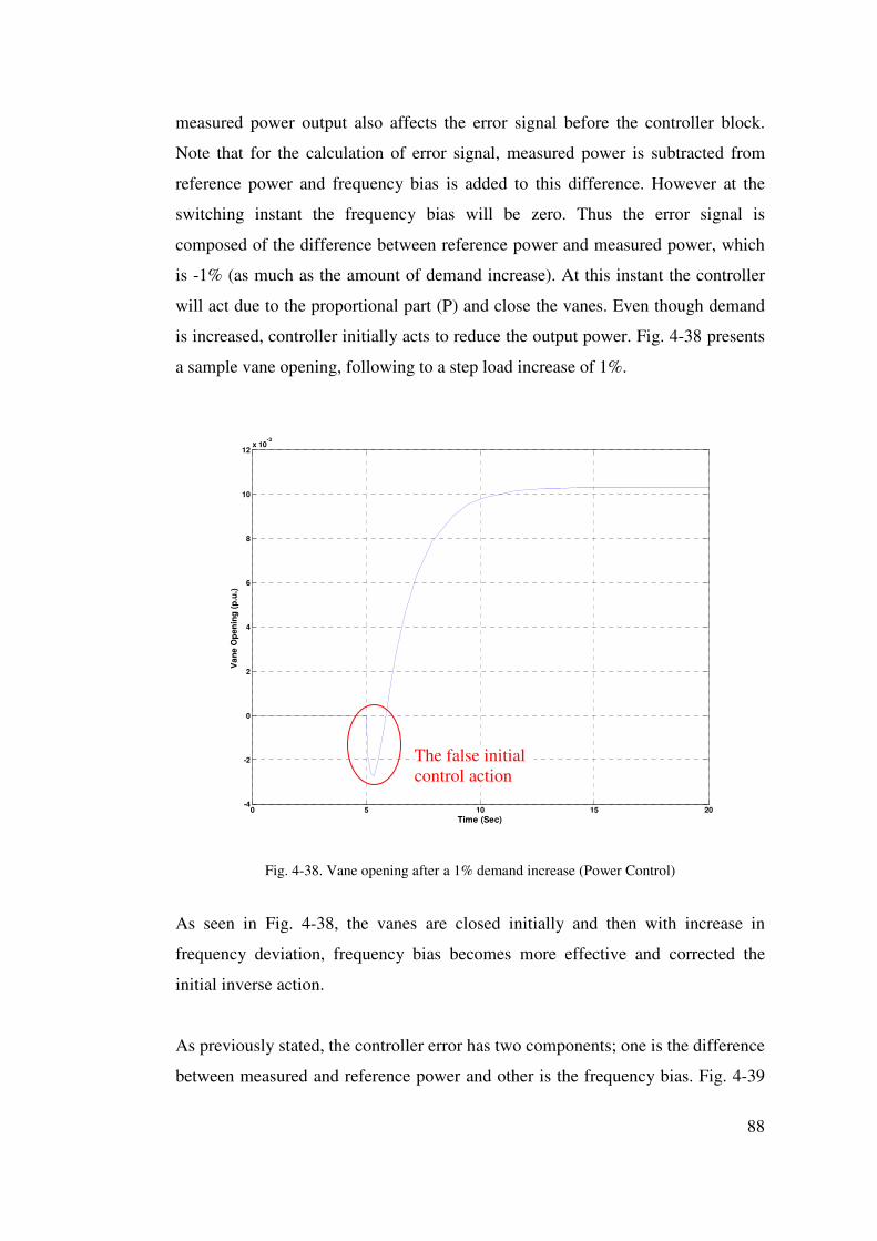
88
measured power output also affects the error signal before the controller block.
Note that for the calculation of error signal, measured power is subtracted from
reference power and frequency bias is added to this difference. However at the
switching instant the frequency bias will be zero. Thus the error signal is
composed of the difference between reference power and measured power, which
is -1% (as much as the amount of demand increase). At this instant the controller
will act due to the proportional part (P) and close the vanes. Even though demand
is increased, controller initially acts to reduce the output power. Fig. 4-38 presents
a sample vane opening, following to a step load increase of 1%.
0 5 10 15 20-4
-2
0
2
4
6
8
10
12x 10
-3
Time (Sec)
Van
e O
pen
ing
(p
.u.)
Fig. 4-38. Vane opening after a 1% demand increase (Power Control)
As seen in Fig. 4-38, the vanes are closed initially and then with increase in
frequency deviation, frequency bias becomes more effective and corrected the
initial inverse action.
As previously stated, the controller error has two components; one is the difference
between measured and reference power and other is the frequency bias. Fig. 4-39
The false initial control action
89
presents these signals for better understanding. As seen in Fig. 4-39, electrical
power deviation is in the form of a step signal since the demand of the island and
power reference of the controller are constants. At the instant of breaker closing
the electrical power deviation introduces a negative step signal to controller input
as seen in Fig. 4-39. Due to this drop, the controller error becomes negative and
gates are closed. Following to this inverse action, with the effect of frequency bias,
the error signal increases and becomes positive and gates are opened in order to
supply increased demand.
0 5 10 15 20-0.02
-0.01
0
0.01
0.02
0.03
0.04
Time (Sec)
Co
ntr
olle
r S
ign
als
(p.u
.)
Controller Error (A)
Electrical Power Deviation (B)
Frequency Bias (C)
Zero Crossing Instant of Controller Error
A
C
B
A = B + C
Fig. 4-39. Controller signal deviations after a 1% demand increase (Power Control)
It should be noted that this false initial control action is directly proportional with
the P value of PI controller. Setting P as zero would immediately solve this
problem. However as seen in Fig. 4-37, setting P to zero makes the unit unstable.
Hence power control without speed control has also a conflict; either the unit will
be unstable or the controller will have a false initial response to power deviations.
It should also be noted that this problem is not only related with HPPs as in the
case of speed controller. This controller structure will create similar problems in
other power plants also.
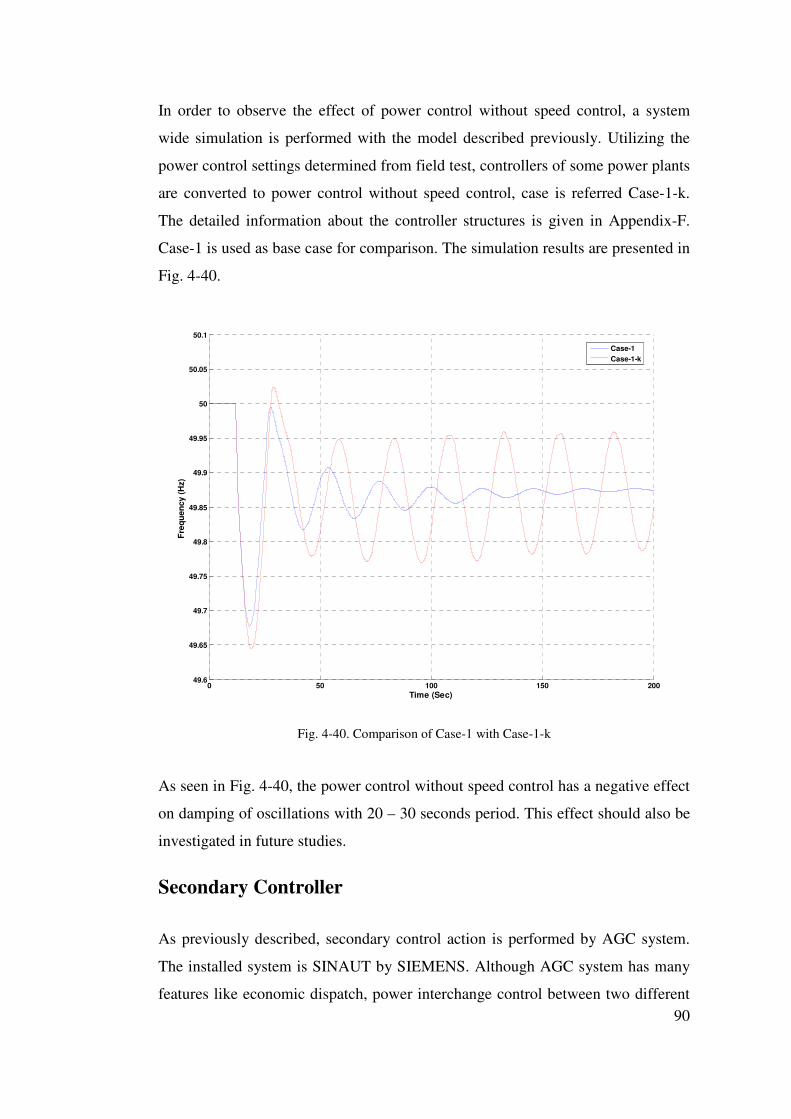
90
In order to observe the effect of power control without speed control, a system
wide simulation is performed with the model described previously. Utilizing the
power control settings determined from field test, controllers of some power plants
are converted to power control without speed control, case is referred Case-1-k.
The detailed information about the controller structures is given in Appendix-F.
Case-1 is used as base case for comparison. The simulation results are presented in
Fig. 4-40.
0 50 100 150 20049.6
49.65
49.7
49.75
49.8
49.85
49.9
49.95
50
50.05
50.1
Time (Sec)
Fre
qu
ency
(H
z)
Case-1
Case-1-k
Fig. 4-40. Comparison of Case-1 with Case-1-k
As seen in Fig. 4-40, the power control without speed control has a negative effect
on damping of oscillations with 20 – 30 seconds period. This effect should also be
investigated in future studies.
Secondary Controller
As previously described, secondary control action is performed by AGC system.
The installed system is SINAUT by SIEMENS. Although AGC system has many
features like economic dispatch, power interchange control between two different
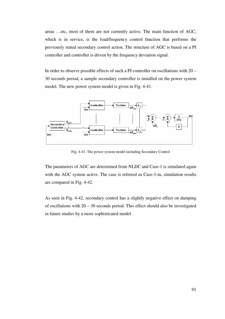
91
areas …etc, most of them are not currently active. The main function of AGC,
which is in service, is the load/frequency control function that performs the
previously stated secondary control action. The structure of AGC is based on a PI
controller and controller is driven by the frequency deviation signal.
In order to observe possible effects of such a PI controller on oscillations with 20 –
30 seconds period, a sample secondary controller is installed on the power system
model. The new power system model is given in Fig. 4-41.
Fig. 4-41. The power system model including Secondary Control
The parameters of AGC are determined from NLDC and Case-1 is simulated again
with the AGC system active. The case is referred as Case-1-m, simulation results
are compared in Fig. 4-42.
As seen in Fig. 4-42, secondary control has a slightly negative effect on damping
of oscillations with 20 – 30 seconds period. This effect should also be investigated
in future studies by a more sophisticated model.
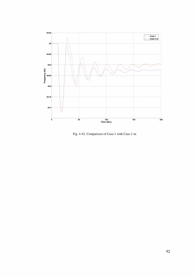
92
0 50 100 150 200
49.7
49.75
49.8
49.85
49.9
49.95
50
50.05
Time (Sec)
Fre
qu
ency
(H
z)
Case-1
Case-1-m
Fig. 4-42. Comparison of Case-1 with Case-1-m
93
C H A P T E R 5
5. CONCLUSION AND FUTURE WORK
This study investigates the effects of hydro power plants’ (HPP) governor settings
on the Turkish power system frequency. For this purpose, the load/frequency
controller accurate mathematical models are developed for two major power plants
which provide considerable primary reserve for frequency regulation in Turkey.
These controller models and parameters are validated by field tests. The unit
controllers of other HPPs are developed based on the manufacturer documentation
provided by the power plant staff. All assumptions made during the modeling are
described in the study. After modeling the unit controllers, a representative power
system model is developed for simulation studies.
The following are the main results determined from the computer simulation
studies;
● The increase in contribution of HPPs with fast speed control settings
(unstable in island operation) to primary frequency control has a negative
effect on damping of frequency oscillations in Turkey. This phenomenon can
be explained as follows; essentially if all controllers in a power system are
stable in island operation, then the interconnected system will be stable. Even
effects of small percentages of unstable controllers can be compensated by
stable controllers. However in case of Turkish power system, reserve of HPPs,
which have unstable controllers, corresponds to approximately 75 % of the
overall reserve. The negative effects of these unstable controllers are
94
eliminated by other plants to some extend depending on their reserve but
essentially the increase in contribution of unstable controllers, negatively
effects the damping of frequency oscillations.
● The increase in speed droop setting (i.e., decreasing the gain) of the HPP
speed controllers has a positive effect on damping of frequency oscillations.
However, this decreases the primary reserve contribution from the HPPs and
increases the system overall speed droop, and therefore, the steady state
frequency deviation will be larger after an event. Although this could be
considered as a trade-off between frequency oscillation and deviation,
frequency deviation is not a major problem. Since the AGC system is in
operation, deviation in frequency will be eliminated by secondary control
action. Hence the increasing speed droop reduces the primary control reserve
and increases the secondary control reserve of HPPs. That is, most of the
primary regulation will be performed by other plants and HPPs will be more
effective in secondary control.
● Changing speed controller parameters (i.e., PI controller parameter) to
make the unit stable in island operation has essentially a positive effect on
damping of oscillations. However, the stable operation settings require less
proportional gain (P) which corresponds to higher temporary droop (RT). With
the effect of higher temporary droop the wicket gates will have a reduced
initial response which will limit the negative effect of the water column in the
penstock. Also reducing the integration gain (I) corresponds to increasing of
reset time constant (TR) which results in slower elimination of temporary droop
effect and hence slower opening of wicket gates. Thus the response of the
overall system becomes sluggish and therefore, the initial frequency deviation
and restoration time increases in case of a disturbance.
● Modification of the speed control structure with including a derivative of
speed deviation input has a positive effect on damping of oscillations.
Currently Birecik, Berke and Keban HPPs are equipped with controllers that
have such an input signal. It is essentially not economical to modify every
95
speed controller structure of HPPs lacking such configuration in Turkey.
However, such modifications could be considered during rehabilitation of old
plants and commissioning of new plants.
One of the main conclusions of the study is that the modification of HPPs’ unit
controller settings to improve response time conflicts with the stable operation of
the units. That is, the controller settings required for stable operation are
contradicting with settings required for a fast primary control response. The grid
code of Turkish power system, which requires fast response (limit is maximum 30
seconds) from HPPs, should consider this conflict. The conclusion of this study
proposes some modifications on the grid code. The load/frequency regulation
performance of the HPPs should be individually evaluated taking into account the
stability limits and characteristics of the individual power plants. In the study, the
required parameter settings of the HPP unit controllers for stable load/frequency
regulation are formulated based on the individual characteristics of the plant
including the penstock, dam, and the generator inertia. These formulations can
give idea to the TEİAŞ authorities in modifying the grid code.
Other factors, which might also have negative effects on frequency, such as
controller structure type (e.g., power controller together with frequency bias) and
AGC (i.e., secondary control), are also discussed in the study. However, only some
preliminary studies are performed. After the preliminary studies it is observed that;
● Power controllers operating without speed controllers have a false initial
response to instant changes in generator power output. That is, in case of an
increase in generator power output the controller responds by closing
regulating vanes initially or vice versa. Note that this effect is not due to inertia
of water or any other property of the plant but a result of the controller
structure. This effect can only be eliminated in the expense of controller
stability. Hence it is concluded that the speed controller loop should always be
active and power controller should be used only to regulate load or speed
reference by the signals supplied from AGC system. Further power control
96
should have relatively slower settings than speed control in order to eliminate
the false initial response.
● The speed droop setting of power controller in operation with speed
controller (i.e., in parallel or cascade) should be chosen carefully. In case of a
different speed droop setting the final primary response of the unit will be
determined by speed droop setting of power controller.
● Future studies could include the investigation of effects of power control
and secondary control on Turkish power system frequency.
Given that the study focuses on the effect of HPP unit controllers, standard models
(mostly IEEE standard models) are used to represent unit controllers of TPPs and
NGCCPPs based on certain assumptions described in the thesis. The basic
assumption is that those power plants’ unit controller settings are set in a way such
that the units are stable in providing frequency regulation. Future studies can deal
with the negative effects (if any) of such power plants on the frequency.
97
REFERENCES
[1] IEEE/CIGRE Joint Task Force on Stability Terms and Definitions,
“Definitions and Classification of Power System Stability”, IEEE Trans. Power
Systems, vol.19, pp. 1387–1399, May 2004.
[2] P. Kundur, Power System Stability and Control, New York: McGraw-Hill,
1994.
[3] “UCTE Operation Handbook”, Union for the Coordination of Transmission of
Electricity, June 2004.
[4] M. E. Cebeci, U. Karaagac, O. B. Tor and A. Ertaş , “The Effects of Hydro
Power Plants’ Governor Settings on the Stability of Turkish Power System
Frequency ” ELECO Conf, Bursa, Turkey, Dec. 2007.
[5] “Complementary Studies for the Synchronization of the Turkish Power System
with the UCTE Power System”, UCTE, May 2007.
[6] J. F. Douglas and R. D. Mathews, Fluid Mechanics, 2. Addison Wesley
Longman Ltd.: 1996.
[7] S. Mansoor, "Behavior and Operation of Pumped Storage Hydro Plants", PhD
Thesis, University of Wales.
98
[8] J. M. Undrill and J. L. Woodward, “Nonlinear Hydro Governing Model and
Improved Calculation for Determining Temporary Droop”, IEEE Trans. Power
Apparatus and Systems, vol. Pas-86, pp. 443–453, Apr. 1967.
[9] F. R. Schleif AND A. B. Wilbor, “The Coordination of Hydraulic Turbine
Governors for Power System Operation”, IEEE Trans. Power Apparatus and
Systems, vol. Pas-85, pp. 750–758, July 1966.
[10] IEEE Working Group on Prime Mover and Energy Supply Models for System
Dynamic Performance Studies, “Hydraulic Turbine and Turbine Control Models
for System Dynamic Studies” IEEE Trans. Power Systems, vol. 7, pp. 167–179,
Feb. 1992.
[11] IEEE Committee Report, “Dynamic Models for Hydro Turbines in Power
System Studies”, IEEE Trans. Power Apparatus and Systems, 1973.
[12] C.D.Vournas and A.Zaharakis, “Hydro Turbine Transfer Functions
with Hydraulic Coupling”, IEEE Trans. Energy Conversion, vol. 8, pp. 527–532,
Sept. 1993.
[13] C. C. Warnick, Hydropower Engineering, Prentice-Hall Ltd., 1984
[14] W. D. Stevenson, Elements of Power System Analysis, New York: McGraw-
Hill, 1986.
[15] Energy Market Regulatory Authority of Turkey,
http://www.epdk.org.tr/mevzuat/yonetmelik/elektrik/sebeke/sebeke.pdf, Jan. 2008.
[16] O. Yılmaz, “Participation of Combined Cycle Power Plants to Power System
Frequency Control: Modeling and Application”, Ms Thesis, Middle East Technical
University, Apr. 2006.

99
[17] L. N. Hannett and B.Fardanesh, “Field Tests to Validate Hydro Turbine
Governor Model Structure and Parameters”, IEEE Trans.Power System, Vol. 9,
pp. 1744–1751, Nov. 1994.
[18] Mathworks Company, www.mathwork.com, Jan. 2008.
[19] Siemens Company, www.pti-us.com, Jan. 2008.
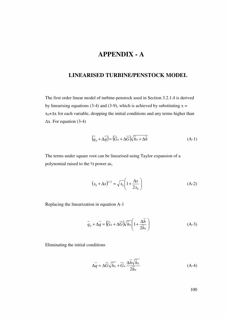
100
APPENDICES
APPENDIX - A
A. LINEARISED TURBINE/PENSTOCK MODEL
The first order linear model of turbine-penstock used in Section 3.2.1.4 is derived
by linearising equations (3-4) and (3-9), which is achieved by substituting x =
x0+∆x for each variable, dropping the initial conditions and any terms higher than
∆x. For equation (3-4)
( ) ( ) hhGGqq ∆+∆+=∆+ 000 (A-1)
The terms under square root can be linearised using Taylor expansion of a
polynomial raised to the ½ power as,
( )
∆+=∆+
0
0
2/1
0 21
x
xxxx (A-2)
Replacing the linearization in equation A-1
( )
∆+∆+=∆+
0
0002
1h
hhGGqq (A-3)
Eliminating the initial conditions
0
000
2h
hhGhGq
∆+∆=∆ (A-4)
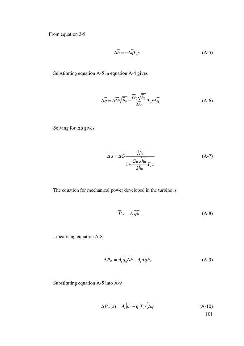
101
From equation 3-9
sTqh w∆−=∆ (A-5)
Substituting equation A-5 in equation A-4 gives
qsTh
hGhGq w ∆−∆=∆
0
000
2 (A-6)
Solving for q∆ gives
sTh
hG
hGq
w0
00
0
21+
∆=∆ (A-7)
The equation for mechanical power developed in the turbine is
hqAP tm = (A-8)
Linearising equation A-8
00 hqAhqAP ttm ∆+∆=∆ (A-9)
Substituting equation A-5 into A-9
( ) qsTqhAsP wtm ∆−=∆ 00)( (A-10)
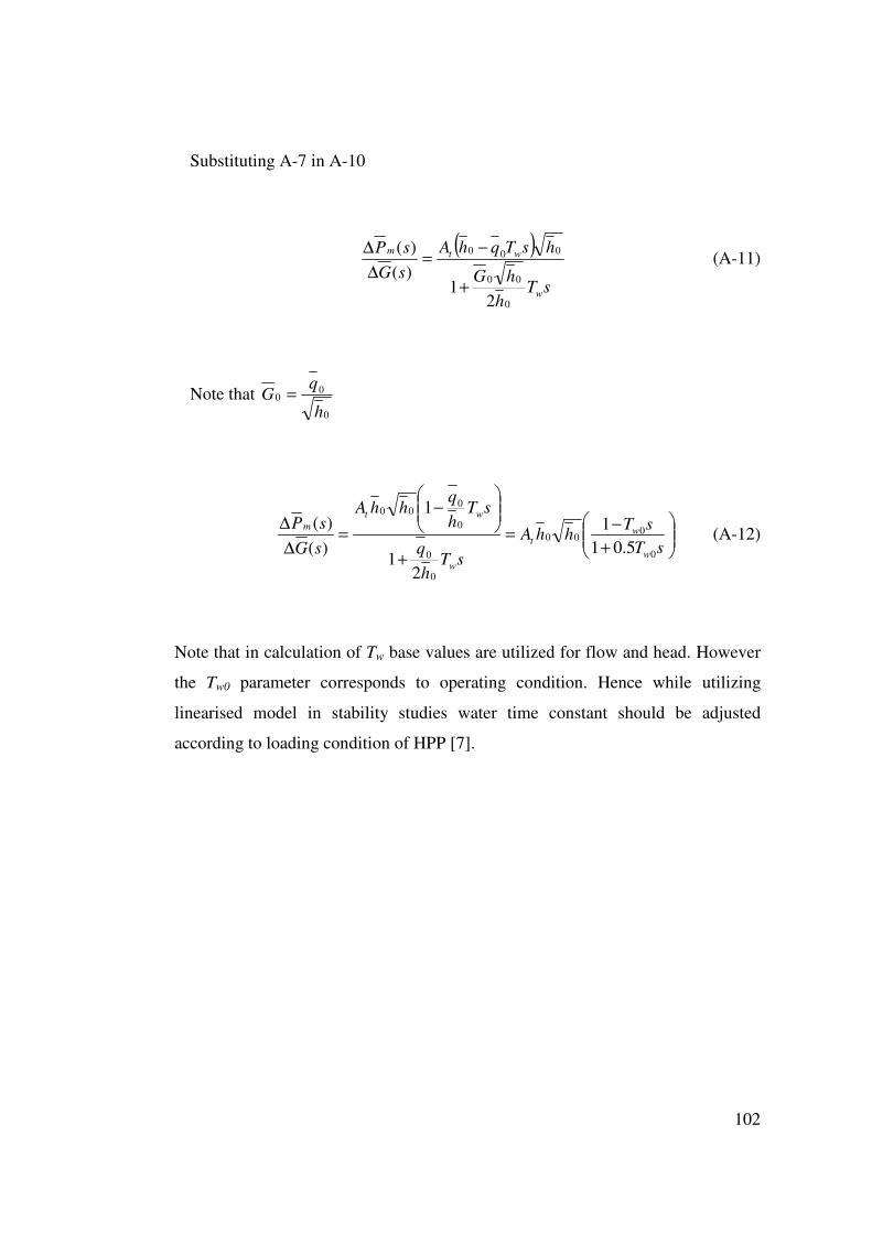
102
Substituting A-7 in A-10
( )
sTh
hG
hsTqhA
sG
sP
w
wtm
0
00
000
21
)(
)(
+
−=
∆
∆ (A-11)
Note that 0
00
h
qG =
+
−=
+
−
=∆
∆
sT
sThhA
sTh
q
sTh
qhhA
sG
sP
w
wt
w
wt
m
0
000
0
0
0
000
5.01
1
21
1
)(
)( (A-12)
Note that in calculation of Tw base values are utilized for flow and head. However
the Tw0 parameter corresponds to operating condition. Hence while utilizing
linearised model in stability studies water time constant should be adjusted
according to loading condition of HPP [7].
103
APPENDIX - B
B. LOAD FLOW SIMULATIONS OF INITIAL CONDITIONS PRIOR TO ISLAND TESTS IN
ATATÜRK AND BIRECIK HYDRO POWER PLANTS
In order to confirm the model generated in Matlab – SIMULINK software, another
simulation study is performed in PSS/E software. PSS/E software requires a load
flow simulation of initial conditions before the dynamic simulations. Hence
network models for islanded regions are prepared for conditions prior to islanding
of Atatürk and Birecik power plants. The required data is supplied by TEİAŞ and
the model is constructed. The results of the load flow study for both tests are given
in Fig. B-1 and Fig. B-2. Utilizing these load flow simulations the Matlab models
of Atatürk and Birecik HPPs are validated by dynamic simulations. The results of
modeling studies are presented in section 4.2.
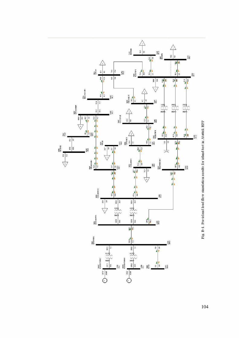
104
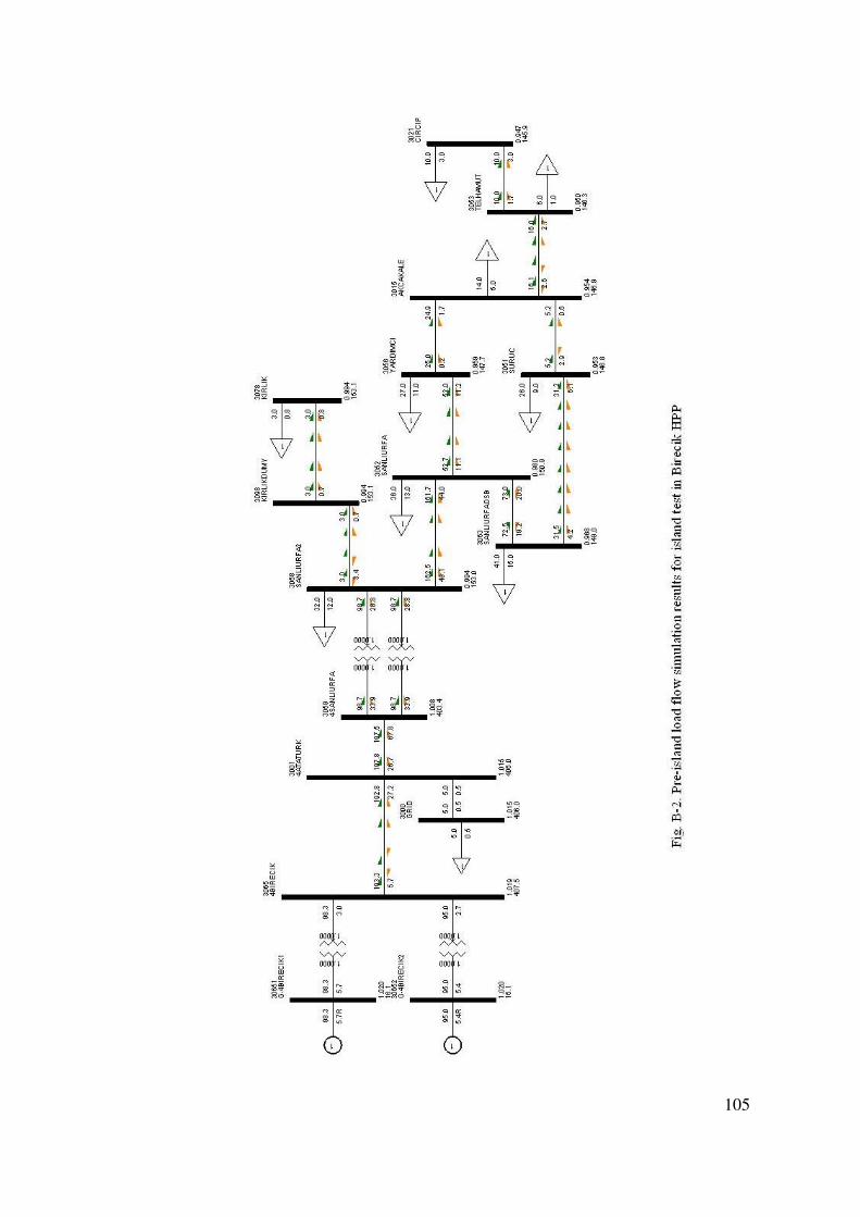
105
106
APPENDIX - C
C. SYSTEM CHARACTERISTIC EQUATION FOR ATATÜRK HYDRO POWER PLANT
The system characteristic equation used in Routh’s test to determine the stability
margins in Section 4.2.4 is derived from equation (4-1) which can be written as,
01)5.01]()([
)1)((=+
+++
−+
sTsTsKsKR
sTKsK
mwIP
wIP (C-1)
Solving equation C-1 yields
s3[0.5RKpTmTw+0.5TmTw]+s
2[RKpTm+Tm+0.5RKITmTw - KpTw]
+s[RKITm+Kp– KITw]+KI = 0 (C-2)
Dividing equation C-2 by Tw2Tm
[ ]
−++
−++++
m
wI
m
wp
wI
wm
wp
wIp
w
p
w T
TK
T
TKTRK
T
s
T
TKTRKRK
T
sRK
T
s2
32
23
5.015.05.0
01 2
4 =
+
m
wI
wT
TK
T (C-3)
Set PRKX =1
wITRKX =2
m
Pw
T
KTX =3
P
wI
K
TKX =4
Multiply both sides by Tw4 and scale snew = s Tw

107
0)()15.0()1(5.0 4343323212
13 =+−+++−+++ XXXXXXsXXXsXs (C-4)
Equation C-4 is used for Routh Hurwitz method.
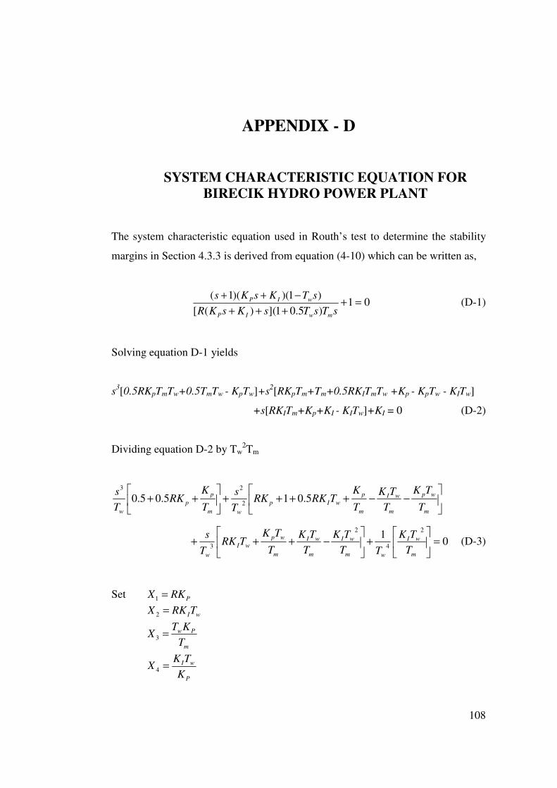
108
APPENDIX - D
D. SYSTEM CHARACTERISTIC EQUATION FOR BIRECIK HYDRO POWER PLANT
The system characteristic equation used in Routh’s test to determine the stability
margins in Section 4.3.3 is derived from equation (4-10) which can be written as,
01)5.01]()([
)1)()(1(=+
+++
−++
sTsTsKsKR
sTKsKs
mwIP
wIP (D-1)
Solving equation D-1 yields
s3[0.5RKpTmTw+0.5TmTw - KpTw]+s
2[RKpTm+Tm+0.5RKITmTw +Kp - KpTw - KITw]
+s[RKITm+Kp+KI - KITw]+KI = 0 (D-2)
Dividing equation D-2 by Tw2Tm
−−++++
++
m
wp
m
wI
m
p
wIp
wm
p
p
w T
TK
T
TK
T
KTRKRK
T
s
T
KRK
T
s5.015.05.0 2
23
01 2
4
2
3 =
+
−+++
m
wI
wm
wI
m
wI
m
wp
wI
wT
TK
TT
TK
T
TK
T
TKTRK
T
s (D-3)
Set PRKX =1
wITRKX =2
m
Pw
T
KTX =3
P
wI
K
TKX =4

109
wTX
15 =
Multiply both sides by Tw4 and scale snew = s Tw
0)(
)15.0(])1(5.0[
435434332
543533212
5313
=++−+
+−++−++++
XXXXXXXXXs
XXXXXXXXsXXXs (D-4)
Equation D-4 is used for Routh Hurwitz method.
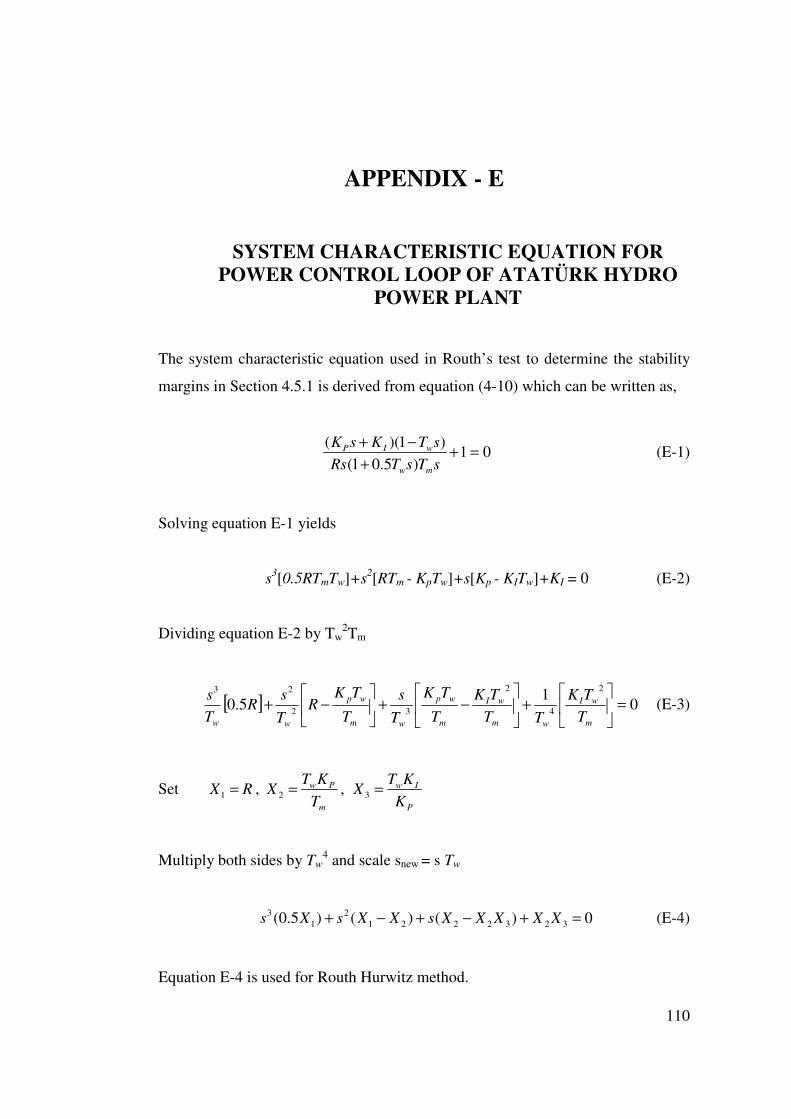
110
APPENDIX - E
E. SYSTEM CHARACTERISTIC EQUATION FOR POWER CONTROL LOOP OF ATATÜRK HYDRO
POWER PLANT The system characteristic equation used in Routh’s test to determine the stability
margins in Section 4.5.1 is derived from equation (4-10) which can be written as,
01)5.01(
)1)((=+
+
−+
sTsTRs
sTKsK
mw
wIP (E-1)
Solving equation E-1 yields
s3[0.5RTmTw]+s
2[RTm - KpTw]+s[Kp - KITw]+KI = 0 (E-2)
Dividing equation E-2 by Tw2Tm
[ ] 01
5.02
4
2
32
23
=
+
−+
−+
m
wI
wm
wI
m
wp
wm
wp
ww T
TK
TT
TK
T
TK
T
s
T
TKR
T
sR
T
s (E-3)
Set RX =1 , m
Pw
T
KTX =2 ,
P
Iw
K
KTX =3
Multiply both sides by Tw
4 and scale snew = s Tw
0)()()5.0( 32322212
13 =+−+−+ XXXXXsXXsXs (E-4)
Equation E-4 is used for Routh Hurwitz method.
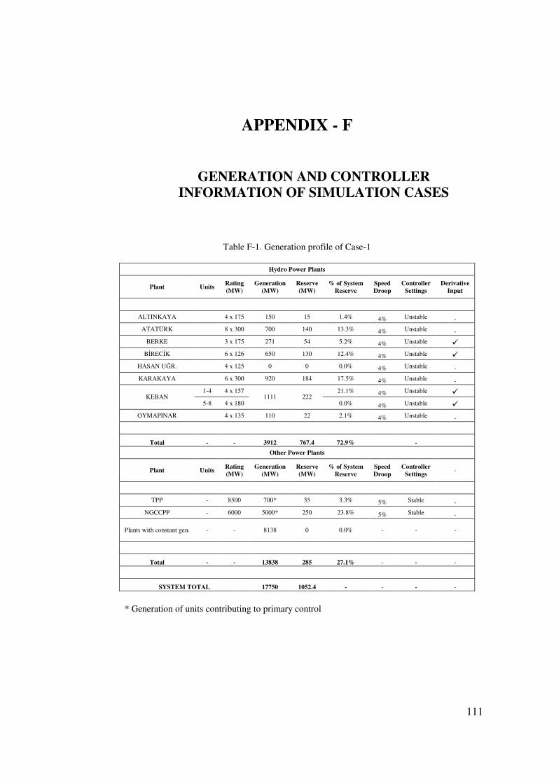
111
APPENDIX - F
F. GENERATION AND CONTROLLER INFORMATION OF SIMULATION CASES
Table F-1. Generation profile of Case-1
Hydro Power Plants
Plant Units Rating (MW)
Generation (MW)
Reserve (MW)
% of System Reserve
Speed Droop
Controller Settings
Derivative Input
ALTINKAYA 4 x 175 150 15 1.4% 4% Unstable -
ATATÜRK 8 x 300 700 140 13.3% 4% Unstable -
BERKE 3 x 175 271 54 5.2% 4% Unstable �
BİRECİK 6 x 126 650 130 12.4% 4% Unstable �
HASAN UĞR. 4 x 125 0 0 0.0% 4% Unstable -
KARAKAYA 6 x 300 920 184 17.5% 4% Unstable -
1-4 4 x 157 21.1% 4% Unstable � KEBAN
5-8 4 x 180 1111 222
0.0% 4% Unstable �
OYMAPINAR 4 x 135 110 22 2.1% 4% Unstable -
Total - - 3912 767.4 72.9% -
Other Power Plants
Plant Units Rating (MW)
Generation (MW)
Reserve (MW)
% of System Reserve
Speed Droop
Controller Settings
-
TPP - 8500 700* 35 3.3% 5% Stable -
NGCCPP - 6000 5000* 250 23.8% 5% Stable -
Plants with constant gen. - - 8138 0 0.0% - - -
Total - - 13838 285 27.1% - - -
SYSTEM TOTAL 17750 1052.4 - - - -
* Generation of units contributing to primary control
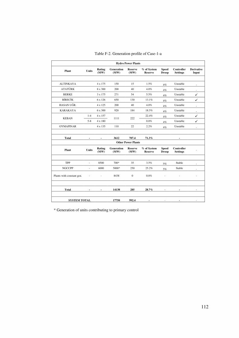
112
Table F-2. Generation profile of Case-1-a
Hydro Power Plants
Plant Units Rating (MW)
Generation (MW)
Reserve (MW)
% of System Reserve
Speed Droop
Controller Settings
Derivative Input
ALTINKAYA 4 x 175 150 15 1.5% 4% Unstable -
ATATÜRK 8 x 300 200 40 4.0% 4% Unstable -
BERKE 3 x 175 271 54 5.5% 4% Unstable �
BİRECİK 6 x 126 650 130 13.1% 4% Unstable �
HASAN UĞR. 4 x 125 200 40 4.0% 4% Unstable -
KARAKAYA 6 x 300 920 184 18.5% 4% Unstable -
1-4 4 x 157 22.4% 4% Unstable � KEBAN
5-8 4 x 180 1111 222
0.0% 4% Unstable �
OYMAPINAR 4 x 135 110 22 2.2% 4% Unstable -
Total - - 3612 707.4 71.3% -
Other Power Plants
Plant Units Rating (MW)
Generation (MW)
Reserve (MW)
% of System Reserve
Speed Droop
Controller Settings
-
TPP - 8500 700* 35 3.5% 5% Stable -
NGCCPP - 6000 5000* 250 25.2% 5% Stable -
Plants with constant gen. - - 8438 0 0.0% - - -
Total - - 14138 285 28.7% - - -
SYSTEM TOTAL 17750 992.4 - - - -
* Generation of units contributing to primary control
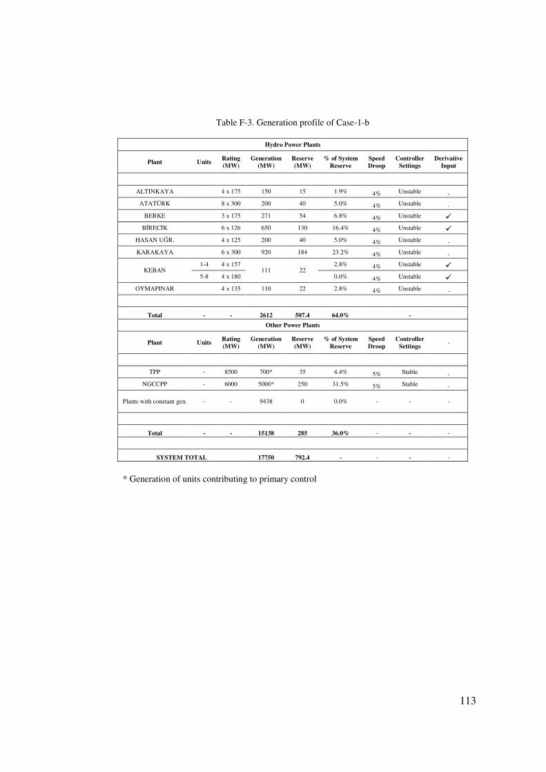
113
Table F-3. Generation profile of Case-1-b
Hydro Power Plants
Plant Units Rating (MW)
Generation (MW)
Reserve (MW)
% of System Reserve
Speed Droop
Controller Settings
Derivative Input
ALTINKAYA 4 x 175 150 15 1.9% 4% Unstable -
ATATÜRK 8 x 300 200 40 5.0% 4% Unstable -
BERKE 3 x 175 271 54 6.8% 4% Unstable �
BİRECİK 6 x 126 650 130 16.4% 4% Unstable �
HASAN UĞR. 4 x 125 200 40 5.0% 4% Unstable -
KARAKAYA 6 x 300 920 184 23.2% 4% Unstable -
1-4 4 x 157 2.8% 4% Unstable � KEBAN
5-8 4 x 180 111 22
0.0% 4% Unstable �
OYMAPINAR 4 x 135 110 22 2.8% 4% Unstable -
Total - - 2612 507.4 64.0% -
Other Power Plants
Plant Units Rating (MW)
Generation (MW)
Reserve (MW)
% of System Reserve
Speed Droop
Controller Settings
-
TPP - 8500 700* 35 4.4% 5% Stable -
NGCCPP - 6000 5000* 250 31.5% 5% Stable -
Plants with constant gen. - - 9438 0 0.0% - - -
Total - - 15138 285 36.0% - - -
SYSTEM TOTAL 17750 792.4 - - - -
* Generation of units contributing to primary control
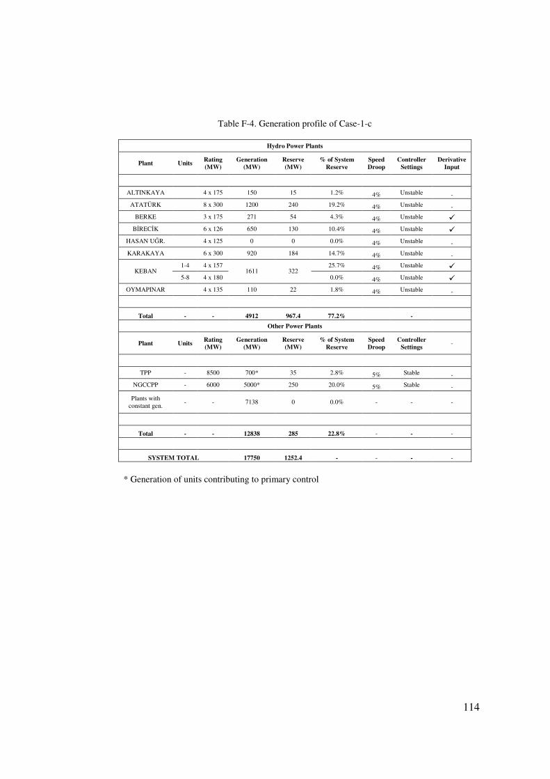
114
Table F-4. Generation profile of Case-1-c
Hydro Power Plants
Plant Units Rating (MW)
Generation (MW)
Reserve (MW)
% of System Reserve
Speed Droop
Controller Settings
Derivative Input
ALTINKAYA 4 x 175 150 15 1.2% 4% Unstable -
ATATÜRK 8 x 300 1200 240 19.2% 4% Unstable -
BERKE 3 x 175 271 54 4.3% 4% Unstable �
BİRECİK 6 x 126 650 130 10.4% 4% Unstable �
HASAN UĞR. 4 x 125 0 0 0.0% 4% Unstable -
KARAKAYA 6 x 300 920 184 14.7% 4% Unstable -
1-4 4 x 157 25.7% 4% Unstable � KEBAN
5-8 4 x 180 1611 322
0.0% 4% Unstable �
OYMAPINAR 4 x 135 110 22 1.8% 4% Unstable -
Total - - 4912 967.4 77.2% -
Other Power Plants
Plant Units Rating (MW)
Generation (MW)
Reserve (MW)
% of System Reserve
Speed Droop
Controller Settings
-
TPP - 8500 700* 35 2.8% 5% Stable -
NGCCPP - 6000 5000* 250 20.0% 5% Stable -
Plants with constant gen.
- - 7138 0 0.0% - - -
Total - - 12838 285 22.8% - - -
SYSTEM TOTAL 17750 1252.4 - - - -
* Generation of units contributing to primary control

115
Table F-5. Generation profile of Case-1-d
Hydro Power Plants
Plant Units Rating (MW)
Generation (MW)
Reserve (MW)
% of System Reserve
Speed Droop
Controller Settings
Derivative Input
ALTINKAYA 4 x 175 150 15 1.0% 4% Unstable -
ATATÜRK 8 x 300 2000 400 27.5% 4% Unstable -
BERKE 3 x 175 271 54 3.7% 4% Unstable �
BİRECİK 6 x 126 650 130 9.0% 4% Unstable �
HASAN UĞR. 4 x 125 200 40 2.8% 4% Unstable -
KARAKAYA 6 x 300 920 184 12.7% 4% Unstable -
1-4 4 x 157 22.2% 4% Unstable � KEBAN
5-8 4 x 180 1611 322
0.0% 4% Unstable �
OYMAPINAR 4 x 135 110 22 1.5% 4% Unstable -
Total - - 5912 1167.4 80.4% -
Other Power Plants
Plant Units Rating (MW)
Generation (MW)
Reserve (MW)
% of System Reserve
Speed Droop
Controller Settings
-
TPP - 8500 700* 35 2.4% 5% Stable -
NGCCPP - 6000 5000* 250 17.2% 5% Stable -
Plants with constant gen.
- - 6138 0 0.0% - - -
Total - - 11838 285 19.6% - - -
SYSTEM TOTAL 17750 1452.4 - - - -
* Generation of units contributing to primary control
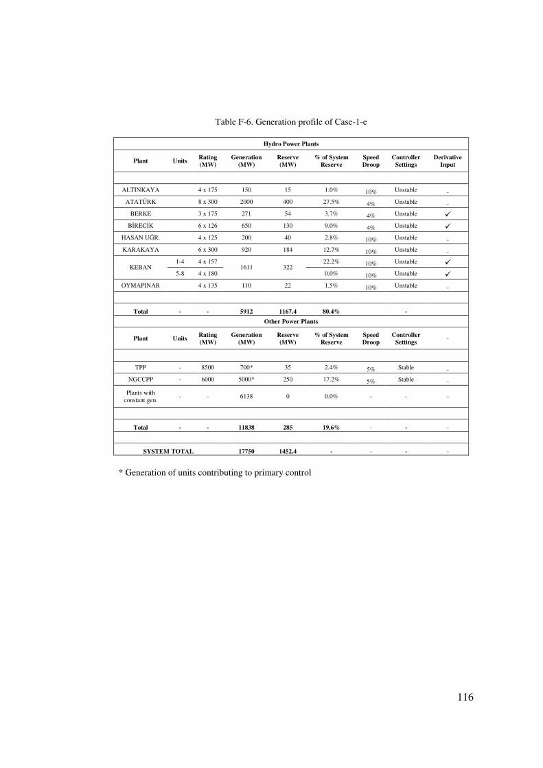
116
Table F-6. Generation profile of Case-1-e
Hydro Power Plants
Plant Units Rating (MW)
Generation (MW)
Reserve (MW)
% of System Reserve
Speed Droop
Controller Settings
Derivative Input
ALTINKAYA 4 x 175 150 15 1.0% 10% Unstable -
ATATÜRK 8 x 300 2000 400 27.5% 4% Unstable -
BERKE 3 x 175 271 54 3.7% 4% Unstable �
BİRECİK 6 x 126 650 130 9.0% 4% Unstable �
HASAN UĞR. 4 x 125 200 40 2.8% 10% Unstable -
KARAKAYA 6 x 300 920 184 12.7% 10% Unstable -
1-4 4 x 157 22.2% 10% Unstable � KEBAN
5-8 4 x 180 1611 322
0.0% 10% Unstable �
OYMAPINAR 4 x 135 110 22 1.5% 10% Unstable -
Total - - 5912 1167.4 80.4% -
Other Power Plants
Plant Units Rating (MW)
Generation (MW)
Reserve (MW)
% of System Reserve
Speed Droop
Controller Settings
-
TPP - 8500 700* 35 2.4% 5% Stable -
NGCCPP - 6000 5000* 250 17.2% 5% Stable -
Plants with constant gen.
- - 6138 0 0.0% - - -
Total - - 11838 285 19.6% - - -
SYSTEM TOTAL 17750 1452.4 - - - -
* Generation of units contributing to primary control

117
Table F-7. Generation profile of Case-1-f
Hydro Power Plants
Plant Units Rating (MW)
Generation (MW)
Reserve (MW)
% of System Reserve
Speed Droop
Controller Settings
Derivative Input
ALTINKAYA 4 x 175 150 15 1.0% 10% Unstable -
ATATÜRK 8 x 300 2000 400 27.5% 10% Unstable -
BERKE 3 x 175 271 54 3.7% 10% Unstable �
BİRECİK 6 x 126 650 130 9.0% 10% Unstable �
HASAN UĞR. 4 x 125 200 40 2.8% 10% Unstable -
KARAKAYA 6 x 300 920 184 12.7% 10% Unstable -
1-4 4 x 157 22.2% 10% Unstable � KEBAN
5-8 4 x 180 1611 322
0.0% 10% Unstable �
OYMAPINAR 4 x 135 110 22 1.5% 10% Unstable -
Total - - 5912 1167.4 80.4% -
Other Power Plants
Plant Units Rating (MW)
Generation (MW)
Reserve (MW)
% of System Reserve
Speed Droop
Controller Settings
-
TPP - 8500 700* 35 2.4% 5% Stable -
NGCCPP - 6000 5000* 250 17.2% 5% Stable -
Plants with constant gen.
- - 6138 0 0.0% - - -
Total - - 11838 285 19.6% - - -
SYSTEM TOTAL 17750 1452.4 - - - -
* Generation of units contributing to primary control

118
Table F-8. Generation profile of Case-1-g
Hydro Power Plants
Plant Units Rating (MW)
Generation (MW)
Reserve (MW)
% of System Reserve
Speed Droop
Controller Settings
Derivative Input
ALTINKAYA 4 x 175 150 15 1.0% 4% Unstable -
ATATÜRK 8 x 300 2000 400 27.5% 4% Stable -
BERKE 3 x 175 271 54 3.7% 4% Stable �
BİRECİK 6 x 126 650 130 9.0% 4% Stable �
HASAN UĞR. 4 x 125 200 40 2.8% 4% Unstable -
KARAKAYA 6 x 300 920 184 12.7% 4% Unstable -
1-4 4 x 157 22.2% 4% Unstable � KEBAN
5-8 4 x 180 1611 322
0.0% 4% Unstable �
OYMAPINAR 4 x 135 110 22 1.5% 4% Unstable -
Total - - 5912 1167.4 80.4% -
Other Power Plants
Plant Units Rating (MW)
Generation (MW)
Reserve (MW)
% of System Reserve
Speed Droop
Controller Settings
-
TPP - 8500 700* 35 2.4% 5% Stable -
NGCCPP - 6000 5000* 250 17.2% 5% Stable -
Plants with constant gen.
- - 6138 0 0.0% - - -
Total - - 11838 285 19.6% - - -
SYSTEM TOTAL 17750 1452.4 - - - -
* Generation of units contributing to primary control
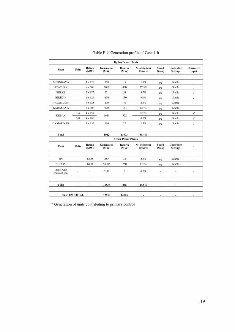
119
Table F-9. Generation profile of Case-1-h
Hydro Power Plants
Plant Units Rating (MW)
Generation (MW)
Reserve (MW)
% of System Reserve
Speed Droop
Controller Settings
Derivative Input
ALTINKAYA 4 x 175 150 15 1.0% 4% Stable -
ATATÜRK 8 x 300 2000 400 27.5% 4% Stable -
BERKE 3 x 175 271 54 3.7% 4% Stable �
BİRECİK 6 x 126 650 130 9.0% 4% Stable �
HASAN UĞR. 4 x 125 200 40 2.8% 4% Stable -
KARAKAYA 6 x 300 920 184 12.7% 4% Stable -
1-4 4 x 157 22.2% 4% Stable � KEBAN
5-8 4 x 180 1611 322
0.0% 4% Stable �
OYMAPINAR 4 x 135 110 22 1.5% 4% Stable -
Total - - 5912 1167.4 80.4% -
Other Power Plants
Plant Units Rating (MW)
Generation (MW)
Reserve (MW)
% of System Reserve
Speed Droop
Controller Settings
-
TPP - 8500 700* 35 2.4% 5% Stable -
NGCCPP - 6000 5000* 250 17.2% 5% Stable -
Plants with constant gen.
- - 6138 0 0.0% - - -
Total - - 11838 285 19.6% - - -
SYSTEM TOTAL 17750 1452.4 - - - -
* Generation of units contributing to primary control

120
Table F-10. Generation profile of Case-1-i
Hydro Power Plants
Plant Units Rating (MW)
Generation (MW)
Reserve (MW)
% of System Reserve
Speed Droop
Controller Settings
Derivative Input
ALTINKAYA 4 x 175 150 15 1.0% 4% Unstable -
ATATÜRK 8 x 300 2000 400 27.5% 4% Unstable �
BERKE 3 x 175 271 54 3.7% 4% Unstable �
BİRECİK 6 x 126 650 130 9.0% 4% Unstable �
HASAN UĞR. 4 x 125 200 40 2.8% 4% Unstable -
KARAKAYA 6 x 300 920 184 12.7% 4% Unstable -
1-4 4 x 157 22.2% 4% Unstable � KEBAN
5-8 4 x 180 1611 322
0.0% 4% Unstable �
OYMAPINAR 4 x 135 110 22 1.5% 4% Unstable -
Total - - 5912 1167.4 80.4% -
Other Power Plants
Plant Units Rating (MW)
Generation (MW)
Reserve (MW)
% of System Reserve
Speed Droop
Controller Settings
-
TPP - 8500 700* 35 2.4% 5% Stable -
NGCCPP - 6000 5000* 250 17.2% 5% Stable -
Plants with constant gen.
- - 6138 0 0.0% - - -
Total - - 11838 285 19.6% - - -
SYSTEM TOTAL 17750 1452.4 - - - -
* Generation of units contributing to primary control

121
Table F-11. Generation profile of Case-1-j
Hydro Power Plants
Plant Units Rating (MW)
Generation (MW)
Reserve (MW)
% of System Reserve
Speed Droop
Controller Settings
Derivative Input
ALTINKAYA 4 x 175 150 15 1.0% 4% Unstable �
ATATÜRK 8 x 300 2000 400 27.5% 4% Unstable �
BERKE 3 x 175 271 54 3.7% 4% Unstable �
BİRECİK 6 x 126 650 130 9.0% 4% Unstable �
HASAN UĞR. 4 x 125 200 40 2.8% 4% Unstable �
KARAKAYA 6 x 300 920 184 12.7% 4% Unstable �
1-4 4 x 157 22.2% 4% Unstable � KEBAN
5-8 4 x 180 1611 322
0.0% 4% Unstable �
OYMAPINAR 4 x 135 110 22 1.5% 4% Unstable �
Total - - 5912 1167.4 80.4% -
Other Power Plants
Plant Units Rating (MW)
Generation (MW)
Reserve (MW)
% of System Reserve
Speed Droop
Controller Settings
-
TPP - 8500 700* 35 2.4% 5% Stable -
NGCCPP - 6000 5000* 250 17.2% 5% Stable -
Plants with constant gen.
- - 6138 0 0.0% - - -
Total - - 11838 285 19.6% - - -
SYSTEM TOTAL 17750 1452.4 - - - -
* Generation of units contributing to primary control
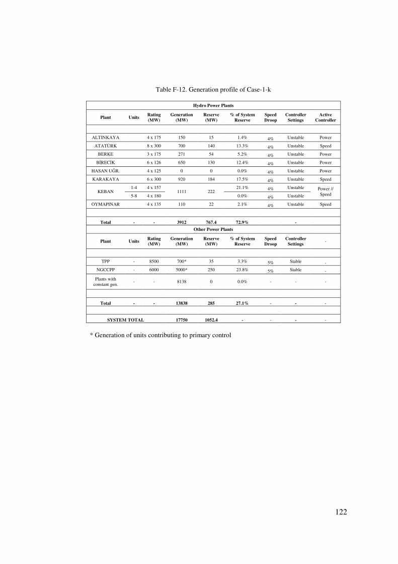
122
Table F-12. Generation profile of Case-1-k
Hydro Power Plants
Plant Units Rating (MW)
Generation (MW)
Reserve (MW)
% of System Reserve
Speed Droop
Controller Settings
Active Controller
ALTINKAYA 4 x 175 150 15 1.4% 4% Unstable Power
ATATÜRK 8 x 300 700 140 13.3% 4% Unstable Speed
BERKE 3 x 175 271 54 5.2% 4% Unstable Power
BİRECİK 6 x 126 650 130 12.4% 4% Unstable Power
HASAN UĞR. 4 x 125 0 0 0.0% 4% Unstable Power
KARAKAYA 6 x 300 920 184 17.5% 4% Unstable Speed
1-4 4 x 157 21.1% 4% Unstable KEBAN
5-8 4 x 180 1111 222
0.0% 4% Unstable
Power // Speed
OYMAPINAR 4 x 135 110 22 2.1% 4% Unstable Speed
Total - - 3912 767.4 72.9% -
Other Power Plants
Plant Units Rating (MW)
Generation (MW)
Reserve (MW)
% of System Reserve
Speed Droop
Controller Settings
-
TPP - 8500 700* 35 3.3% 5% Stable -
NGCCPP - 6000 5000* 250 23.8% 5% Stable -
Plants with constant gen.
- - 8138 0 0.0% - - -
Total - - 13838 285 27.1% - - -
SYSTEM TOTAL 17750 1052.4 - - - -
* Generation of units contributing to primary control

123
Table F-13. Generation profile of Case-2
Hydro Power Plants
Plant Units Rating (MW)
Generation (MW)
Reserve (MW)
% of System Reserve
Speed Droop
Controller Settings
Derivative Input
ALTINKAYA 4 x 175 300 50 5.4% 4% Unstable -
ATATÜRK 8 x 300 1000 200 21.6% 4% Unstable -
BERKE 3 x 175 300 50 5.4% 4% Unstable �
BİRECİK 6 x 126 300 78 8.4% 4% Unstable �
HASAN UĞR. 4 x 125 100 25 2.7% 4% Unstable -
KARAKAYA 6 x 300 550 50 5.4% 4% Unstable -
1-4 4 x 157 360 100 10.8% 4% Unstable � KEBAN
5-8 4 x 180 600 120 12.9% 4% Unstable �
OYMAPINAR 4 x 135 0 0 0.0% 4% Unstable -
Total - - 3510 673 72.5% -
Other Power Plants
Plant Units Rating (MW)
Generation (MW)
Reserve (MW)
% of System Reserve
Speed Droop
Controller Settings
-
TPP - 8500 600* 30 3.2% 5% Stable -
NGCCPP - 6000 4500* 225 24.2% 5% Stable -
Plants with constant gen.
- - 11390 0 0.0% - - -
Total - - 16490 255 27.5% - - -
SYSTEM TOTAL 20000 928 - - - -
* Generation of units contributing to primary control

124
Table F-14. Generation profile of Case-3
Hydro Power Plants
Plant Units Rating (MW)
Generation (MW)
Reserve (MW)
% of System Reserve
Speed Droop
Controller Settings
Derivative Input
ALTINKAYA 4 x 175 300 50 3.9% 4% Unstable -
ATATÜRK 8 x 300 1550 250 19.5% 4% Unstable -
BERKE 3 x 175 475 50 3.9% 4% Unstable � BİRECİK 6 x 126 650 100 7.8% 4% Unstable �
HASAN UĞR. 4 x 125 100 25 2.0% 4% Unstable -
KARAKAYA 6 x 300 1375 125 9.8% 4% Unstable -
1-4 4 x 157 360 100 7.8% 4% Unstable � KEBAN
5-8 4 x 180 600 120 9.4% 4% Unstable �
OYMAPINAR 4 x 135 355 50 3.9% 4% Unstable -
Total - - 5765 870 68.0% -
Other Power Plants
Plant Units Rating (MW)
Generation (MW)
Reserve (MW)
% of System Reserve
Speed Droop
Controller Settings
-
TPP - 8500 700* 35 2.7% 5% Stable -
NGCCPP - 6000 5000* 250 19.5% 5% Stable -
Plants with constant gen.
- - 8735 0 0.0% - - -
Total - - 14435 285 22.3% - - -
SYSTEM TOTAL 21500 1280 - - - -
* Generation of units contributing to primary control