the effect of the drake passage and subgrid-scale eddy ... · the effect of the drake passage and...
TRANSCRIPT

The effect of the Drake Passage and subgrid-scaleeddy parametrization on the global thermohaline
circulation
Willem P. Sijp
Centre for Environmental Modelling and Prediction, School of Mathematics, University of
New South Wales, Sydney, New South Wales, Australia
February 27, 2006
PhD. Thesis

The effect of the Drake Passage and subgrid-scaleeddy parametrization on the global thermohaline
circulation
Willem P. Sijp
Centre for Environmental Modelling and Prediction, School of Mathematics, University of
New South Wales, Sydney, New South Wales, Australia
Submitted for the degree of Doctor of Philosophy in Science at The University of New
South Wales, Sydney, Australia
February 27, 2006
Acknowledgements
This thesis has gained great benefit from a range of scientific, technical and ad-
ministrative support over the last three and a half years. I greatly acknowledge
the important role that the people involved have played and am very thankful and
appreciative of their sustained support, collaboration and advise. In particular, I
thank Matthew England for his excellent supervision during my candidature. His
encouragement was critically important to the success of this project. Furthermore,
our many discussions about the project have proven to be very fruitful as they en-
couraged critical thinking and have been invaluable to the quality of the end-result
and the rate of progress of the project. I also gratefully acknowledge a number
of researchers for their helpful discussions. In particular, Andreas Schmittner and
Oleg Saenko for discussions during my stay at the University of Victoria that facili-
tated the inception of the study described in chapter 4, now published in the Journal
of Climate (Sijp and England 2005). A short discussion with Anand Gnanade-
sikan and Robbie Toggweiler who kindly hosted my visit at GFDL Princeton and
Cecilia Bitz at the University of Washington about the role of vertical mixing in
my Drake Passage results during a talk encouraged me to include the parameter
study of chapter 5. This project required state of the art computing facilities for
its many equilibrium runs and perturbation experiments. We thank the Australian
Partnership for Advanced Computing (APAC) National Facility for its generous al-
location of computing resources. Furthermore, we greatfully acknowledge the use
of the Matrix Linux Cluster at the School of Mathematics at the University of New
South Wales. We thank Andrew Weaver and the climate group at the University of
Victoria for their support and our usage of the their coupled climate model. Fur-
thermore, we thank the staff at GFDL for making their ocean model MOM version
2.2 Pacanowski (1995) available to the oceanographic community. The author also
acknowledges the financial support of the Australian Postgraduate Award (APA),
the APA top-up scholarship and the School of Mathematics Research Scholarship.
Furthermore, I thank Andrew Weaver and the University of Victoria for hosting my
i

stay there in May 2001. I also thank the School of Mathematics at the University
of New South Wales for funding this visit. Finally, I gratefully acknowledge the
wonderful support of my parents in particular, and my friends and family.
This research also received support from the Australian Research Council and the
Australian Antarctic Science Program.
ii
Supporting publications
Sijp, W.P., and M.H. England, 2005: Sensitivity of the Atlantic thermohaline cir-
culation to basin-scale variations in vertical mixing and its stability to fresh water
perturbations. J. Climate, submitted.
Sijp, W.P, M. Bates and M.H. England, 2005: Can isopycnal mixing control the sta-
bility of the thermohaline circulation in ocean climate models? J. Climate, accepted
subject to revisions.
Sijp, W.P., and M.H. England, 2005: On the role of the Drake Passage in controlling
the stability of the ocean’s thermohaline circulation. J. Climate, 18, 1957-1966.
Sijp, W.P, and M.H. England, 2004: Effect of the Drake Passage throughflow on
global climate, J. Phys. Oceanogr., 34, 1254-1266.
Bates, M.L., M.H. England, and W.P. Sijp, 2005: On the multi-century Southern
Hemisphere response to changes in atmospheric CO2 concentration in a global cli-
mate model. Met. Atmos. Physics, 89, 17-36.
iii

Abstract
We investigate a variety of factors affecting global thermohaline circulation (THC)
stability using a global intermediate complexity coupled model. We find a variety
of implications for past climates and uncovered new uncertainties in the THC re-
sponse to high latitude freshening. In particular, we examine the role of a Southern
Ocean gateway in global climate and the global ocean THC by running a series of
experiments using coupled model where the depth of Drake Passage (DP) varies.
Necessary conditions for the existence of multiple equilibria in the THC are stud-
ied. The climate with DP closed is characterised by warmer Southern Hemisphere
Surface Air Temperature (SAT) and little Antarctic ice. North Antlantic Deep Water
(NADW) overturn is supressed by strong Antarctic Bottom Water (AABW) forma-
tion. Deepening DP gradually removes the influence of the Southern cell until the
model admits a Northern Hemisphere overturning state. To examine the robustness
of some of these results, we discuss a series of experiments where we vary the rate
of vertical mixing and introduce the eddy-parametrisation of Gent and McWilliams
(GM). Furthermore, in Ocean General Circulation Models (OGCMs), a strong re-
duction in convective penetration depth arises when horizontal diffusion (HD) is
replaced by GM mixing to model the effect of mesoscale eddies on tracer advec-
tion. In areas of sinking, the role of vertical tracer transport due to convection
is largely replaced by the vertical component of isopycnal diffusion along sloping
isopycnals. Here, we examine the effect of this change in tracer transport physics on
the stability of NADW formation under fresh water (FW) perturbations of the North
Atlantic in a coupled model. We find a significantly increased stability of NADW
to FW input when GM is used in spite of GM experiments exhibiting consistently
weaker NADW formation rates in unperturbed steady states. Also, we show that
a reduction in vertical mixing coefficient Kv applied inside the Atlantic basin can
drastically increase NADW stability with respect to FW perturbations applied to the
North Atlantic. This is contrary to the notion that the ocean’s meridional overturn-
ing circulation simply scales with vertical mixing rates.
iv

Originality statement
I hereby declare that this submission is my own work and that to the best of my
knowledge it contains no materials previously published or written by another per-
son, or substantial proportions of material which have been accepted for the award
of any other degree or diploma at UNSW or any other educational institution, except
where due acknowledgement is made in the thesis. Any contribution made to the
research by others, with whom I have worked at UNSW or elsewhere, is explicitly
acknowledged in the thesis. I also declare that the intellectual content of this thesis
is the product of my own work, except to the extent that assistance from others in
the project’s design and conception in style, presentation and linguistic expression
is acknowledged.
v

Contents
1 Introduction 1
2 Model 6
3 Steady state: the effect of the Drake Passage throughflow on global
climate 10
3.1 Abstract . . . . . . . . . . . . . . . . . . . . . . . . . . . . . . . . 10
3.2 Introduction . . . . . . . . . . . . . . . . . . . . . . . . . . . . . . 12
3.3 Model description and experimental design . . . . . . . . . . . . . 15
3.4 Ocean circulation response . . . . . . . . . . . . . . . . . . . . . . 16
3.5 Sea-ice response . . . . . . . . . . . . . . . . . . . . . . . . . . . . 21
3.6 Atmospheric response . . . . . . . . . . . . . . . . . . . . . . . . . 22
3.7 Comparison with previous studies . . . . . . . . . . . . . . . . . . 23
3.8 Discussion and Conclusions . . . . . . . . . . . . . . . . . . . . . 27
vi

4 Transient behaviour: the role of Drake Passage in controlling the sta-
bility of the ocean’s thermohaline circulation 39
4.1 Abstract . . . . . . . . . . . . . . . . . . . . . . . . . . . . . . . . 39
4.2 Introduction . . . . . . . . . . . . . . . . . . . . . . . . . . . . . . 40
4.3 Methodology . . . . . . . . . . . . . . . . . . . . . . . . . . . . . 42
4.4 Overturning diagnostics . . . . . . . . . . . . . . . . . . . . . . . . 43
4.5 Results . . . . . . . . . . . . . . . . . . . . . . . . . . . . . . . . . 44
a NADWoff states . . . . . . . . . . . . . . . . . . . . . . . 44
b Response to FW perturbations . . . . . . . . . . . . . . . . 48
c Sensitivity to model experimental design . . . . . . . . . . 50
4.6 Discussion . . . . . . . . . . . . . . . . . . . . . . . . . . . . . . . 51
4.7 Conclusions . . . . . . . . . . . . . . . . . . . . . . . . . . . . . . 54
5 Effect of subgrid-scale eddy parametrization on the Drake Passage/
North Atlantic teleconnection 67
5.1 Abstract . . . . . . . . . . . . . . . . . . . . . . . . . . . . . . . . 67
5.2 Introduction . . . . . . . . . . . . . . . . . . . . . . . . . . . . . . 68
5.3 Model and Experimental Design . . . . . . . . . . . . . . . . . . . 70
5.4 Results . . . . . . . . . . . . . . . . . . . . . . . . . . . . . . . . . 71
a Sensitivity of MOC to vertical mixing . . . . . . . . . . . . 71
vii

b Sensitivity of the DPopen-DPclsd results to mixing parametri-
sation . . . . . . . . . . . . . . . . . . . . . . . . . . . . . 78
5.5 Discussion and Conclusions . . . . . . . . . . . . . . . . . . . . . 83
6 Can isopycnal mixing control the stability of the thermohaline circula-
tion in ocean climate models? 98
6.1 Abstract . . . . . . . . . . . . . . . . . . . . . . . . . . . . . . . . 98
6.2 Introduction . . . . . . . . . . . . . . . . . . . . . . . . . . . . . . 99
6.3 Model and Experimental Design . . . . . . . . . . . . . . . . . . . 104
6.4 Results . . . . . . . . . . . . . . . . . . . . . . . . . . . . . . . . . 105
a Steady state experiments . . . . . . . . . . . . . . . . . . . 105
b Hysteresis behaviour . . . . . . . . . . . . . . . . . . . . . 107
c Transient FW pulse experiments . . . . . . . . . . . . . . . 109
d Diagnosis of model processes . . . . . . . . . . . . . . . . 112
6.5 Discussion and Conclusions . . . . . . . . . . . . . . . . . . . . . 116
7 Sensitivity of the Atlantic thermohaline circulation to basin-scale vari-
ations in vertical mixing and its stability to fresh water perturbations 132
7.1 Abstract . . . . . . . . . . . . . . . . . . . . . . . . . . . . . . . . 132
7.2 Introduction . . . . . . . . . . . . . . . . . . . . . . . . . . . . . . 133
7.3 Model and Numerical Experiments . . . . . . . . . . . . . . . . . . 136
viii

7.4 Results . . . . . . . . . . . . . . . . . . . . . . . . . . . . . . . . . 137
7.5 Conclusions . . . . . . . . . . . . . . . . . . . . . . . . . . . . . . 142
8 Concluding remarks 151
ix

Chapter 1
Introduction
This study focuses on the effect of ocean gateways and subgrid-scale eddy parametri-
sations on global meridional overturning circulation (MOC) strength and stability.
This thesis is divided in two parts. The first part consists of Chapters 3, 4 and 5, and
covers an analysis of the effect of Drake Passage (DP) on global climate. In particu-
lar, the strength, polarity and stability of the global thermohaline circulation (THC)
are examined. A sensitivity analysis of these results with respect to subgrid-scale
mixing parametrisations is also included. The second part consists of Chapters 6
and 7, and covers an analysis of the effect of subgrid-scale mixing parametrisations
on the THC stability.
The study described in Chapter 3 aims to examine the climatic effect of opening DP
and corresponds to the manuscript titled “Effect of the Drake Passage throughflow
on global climate” published as an article in the Journal of Physical Oceanography
(Sijp and England 2004). Although similar previous studies (e.g. Mikolajewicz
et al. 1993; Toggweiler and Bjornsson 2000; Nong et al. 2000) have been conducted,
ours is the first to employ a coupled climate model including sea-ice and a seasonal
cycle using realistic present day topography. We also offer an overview and clas-
sification of previous modelling results. This study is relevant to the interpretation
1

of paleoclimatic data of the Eocene-Oligocene boundary around 33 million years
ago as it was during this period that a circumpolar ocean formed around Antarctica
and the West-Antarctic ice-sheet appeared, heralding a cooling of global climate.
The concurrency of these events was noted by Kennett (1977). Based on field data
that had become available at the time, he proposed that it was the re-arrangement of
ocean currents arising from the opening of all southern ocean gateways that caused
the glaciation of Antarctica, which in turn brought about further global cooling.
Our study gives some support to this hypothesis. In particular, our results allow an
assessment of summer temperature changes around Antarctica, a factor critical to
the build-up of a terrestrial ice-sheet. Changes in ocean currents are not the only
possible cause for Eocene warmth under consideration as can be seen from a re-
cent study by DeConto and Pollard (2004), who stress the importance of higher
atmospheric concentrations of CO2.
To further examine the nature of the thermohaline circulation in the closed and shal-
low DP experiments described in Chapter 3, we have conducted the study described
in Chapter 4. This Chapter contains a somewhat extended version of the manuscript
“On the role of the Drake Passage in controlling the stability of the ocean’s ther-
mohaline circulation” published as an article in the Journal of Climate (Sijp and
England 2005). Here we elucidate the relation between DP depth and North Ant-
lantic Deep Water (NADW) stability with respect to FW perturbations applied to
the North Atlantic. Combining a range of topographies and fresh water (FW) per-
turbations, this is the first analysis of its kind. It is discovered that no transitions to a
Northern Hemisphere overturning state can occur when the DP sill is shallower than
a critical depth (1100m in our model). This preference for Southern Hemisphere
sinking is a result of the particularly cold conditions of the Antarctic Bottom Wa-
ter (AABW) formation regions compared to the Northern Hemisphere deepwater
formation zones. Upon the introduction of a sufficiently deep DP gap, ocean venti-
lation of Antarctic Intermediate Water (AAIW) occurs to depths of around 1000m
(e.g. Cox 1989). Saenko et al. (2003) demonstrate the importance of the relationship
2

between densities in the AAIW formation regions and those in the NADW forma-
tion regions in determining the MOC and observe that the SH overturning state in a
DP open geometry consists of an AAIW reverse cell where AAIW upwells into the
Atlantic thermocline. We find that the cell of the SH overturning state transforms
gradually from the AABW cell of the DP closed geometry to the AAIW reverse cell
of DP open (and deep) geometry upon deepening DP. The mechanism behind this
transformation lies in a north-south bifurcation of AAIW sinking north of DP.
The climatic changes arising from the opening of DP described in Chapters 3 and
4 are in part related to a fundamental reorganisation of the global MOC. It is well
known (e.g. Bryan 1987), however, that the strength of the global MOC is a function
of the rate of vertical mixing in the thermocline. Furthermore, the rate of NADW
formation is known to be sensitive to the choice of parametrisation of tracer trans-
port by subgrid-scale eddies (e.g. Duffy et al. 1997; England and Holloway 1998).
Therefore, we examine in Chapter 5 the sensitivity of our results to the introduc-
tion of the parametrisation of Gent and McWilliams (1990, GM) and to the rate of
vertical mixing.
The global MOC plays an important role in the studies described in Chapters 3 and
4. In particular, the model response to the FW perturbations applied to the NA is not
only determined by global factors such as topography, but also local factors such
as along isopycnal mixing in the NADW formation regions. It is therefore impor-
tant to examine how results such as those found in Chapter 4 might change due to
changes in parametrisations of these local processes that affect deepwater forma-
tion. In Chapter 6 we therefore examine the effect of along isopycnal mixing on
NADW stability and find a significant increase in FW threshold required to obtain
a transition to a collapsed NADW state when along isopycnal mixing is used. This
result has wider implications and uncovers an uncertainty in estimations of the FW
threshold required to shut down NADW in ocean models in general. For instance,
it has consequences for the interpretation of model THC collapse in response to
3

a freshening of the NA due to an increased vigour of the hydrological cycle and
melt-runoff from a melting terrestrial ice-sheet in climate change experiments. We
find that in areas of sinking, the role of vertical tracer transport due to convection
is largely replaced by the vertical component of isopycnal diffusion along sloping
isopycnals. Upon examining the effect of this change in tracer transport physics on
the stability of NADW formation under FW perturbations of the NA in a coupled
model, we find a significantly increased stability of NADW to FW input when GM
is used in spite of GM experiments exhibiting consistently weaker NADW forma-
tion rates in unperturbed steady states.This manuscript, titled “Can isopycnal mix-
ing control the stability of the thermohaline circulation in ocean climate models?”,
is currently under review with the Journal of Climate.
The AAIW reverse cell examined in Chapter 4 plays an important role in the contin-
ued suppression of NH sinking in the collapsed NADW states there. To examine the
dynamics of this important cell we have conducted a series of experiments described
in Chapter 7 where we decrease vertical mixing only inside the Atlantic basin. This
results in a reduced potential for AAIW to upwell into the Atlantic thermocline. As
this cell is required for the stability of the collapsed NADW state, hampering its
upwelling branch inside the Atlantic reduces the stability of the collapsed NADW
state. Indeed, we find significantly higher FW perturbation thresholds required to
shut down NADW. This is counter-intuitive in a sense, as we demonstrate that we
can increase NADW stability while at the same time reducing the average rate of
vertical mixing in the world ocean. This manuscript, titled “Sensitivity of the At-
lantic thermohaline circulation to basin-scale variations in vertical mixing and its
stability to fresh water perturbations”, is currently in review with the Journal of
Climate.
In these studies we have used the Earth System Climate Model of intermediate
complexity of Weaver et al. (2001, the ”UVic Model”) described in Chapter 2. This
model is ideally suited to the studies we have conducted. The gain in computational
4

speed derived from its simplified atmosphere allowed us to examine a wider range
of scenarios where we vary topography and the magnitude of FW perturbations, yet
the ocean component (GFDL MOM 2.2, Pacanowski 1995) is of sufficiently high
resolution to allow highly detailed simulations. The experiments in Chapters 3 and
4 were conducted using Version 2.5 of the UVic Model. During the course of the
project the newer and computationally more efficient Version 2.6 became available
and we use this version in the remaining Chapters. For our intents and purposes the
versions do not differ significantly in terms of model climate.
The first part of this thesis (Chapters 3, 4 and 5) is best read as one study, whereas
the Chapters in the second part (6 and 7) can be read in isolation. The study de-
scribed in Chapter 3 justifies the study of Chapters 4 and 5 and the three studies
share a common theme, that is the climatic impact of opening the Drake Passage.
The studies described in the second part have implications for the interpretation of
the results of Chapter 4 in the first part. Factors affecting the ocean’s global MOC
form a common thread throughout this thesis. The figures for each chapter appear
at the end of each chapter.
5

Chapter 2
Model
The simulations have been carried out using the Earth System Climate Model of
intermediate complexity of Weaver et al. (2001). The model comprises an ocean
general circulation model coupled to an atmospheric model. A hydrological cycle
with river basins configured over a realistic geometry and a dynamic/ thermody-
namic sea-ice model are included. All components of the model have a global
domain with horizontal resolution 3.6◦by 1.8◦in longitude and latitude respectively.
There are 19 vertical levels in the ocean and no layering in the sea-ice model.
The ocean component of the coupled model is the GFDL Modular Ocean Model
version 2.2 (MOM Pacanowski 1995). MOM is based on the Navier Stokes equa-
tions subject to the Boussinesq and hydrostatic approximations. We employ con-
stant , horizontal viscosity of 2.0×109 cm2 s−1, and vertical viscosity of 10 cm2s−1.
Vertical mixing is achieved through a modified form of the Bryan and Lewis (1979)
vertical distribution, Figure 2.1 shows this vertical distribution of Kv as a func-
tion of depth from the surface of the ocean. Kv ranges from Kv=0.6 cm2 s−1 in
the upper ocean to Kv=1.6 cm2s−1 in the deep ocean. Brine rejection during sea-
ice formation is parametrised after Duffy and Caldeira (1997). Surface forcing is
accomplished using wind stresses calculated from wind fields in the atmospheric
6

component, and ice-air-sea heat and freshwater fluxes. Subgrid-scale mixing varies
by experiment. We either the standard horizontal/ vertical diffusive approach, the
parametrisation of along isopycnal diffusion (ISO, Redi 1982) or eddy induced ad-
vective tracer transport in combination with along-isopycnal diffusion (Gent and
McWilliams 1990). In the standard horizontal diffusive approach (HD), horizontal
diffusivity of 2.0 × 107 cm2 s−1 is used and no along isopycnal diffusion or isopy-
cnal thickness diffusion is used. For eddy-induced advection parametrisation of
Gent and McWilliams (GM, Gent and McWilliams 1990), we use isopycnal thick-
ness diffusion with a constant coefficient of 1×107cm2/s. In GM and ISO we use
isopycnal diffusion with a constant coefficient of 2 × 107cm2/s.
The atmospheric model consists of a 2D energy balance model based on Fanning
and Weaver (1996). The model has one vertical layer. The model allows for redistri-
bution of thermal energy and moisture content through a single vertically-integrated
equation for each. Moisture transports are accomplished through advection (by
wind) and Fickian diffusion. Wind fields act on the ocean through the calculation
of a wind stress. Wind also influences evaporation rates, heat fluxes to the ocean,
and moisture advection. Precipitation is assumed to occur when relative humid-
ity is greater than 85 percent. Precipitation that falls over land is returned to the
ocean instantaneously via prescribed river basins. The wind field is not determined
exclusively by prognostic equations for momentum conservation, but are based on
specific wind data taken from NCEP/NCAR reanalysis (Kalnay et al. 1996, et. al.),
averaged over the period 1958-1997 to form an annual cycle from the monthly
fields. A dynamical wind feedback is included in the form of a term that indicates
the departure from the mean field. Wind feedbacks are calculated from temperature
changes from a mean climatology using a latitudinally dependent relationship be-
tween temperature and air density. While air-sea heat and freshwater fluxes evolve
freely in the model, we employ a non-interactive wind field unless stated otherwise.
Transport of heat is not accomplished through advection, only through Fickian dif-
fusion. Indirectly, advective heat transport can occur through the transport of mois-
7

ture in the atmosphere and consequent precipitation whereby latent heat is released.
Model atmospheric temperatures decrease over uplifted land areas according to a
fixed lapse rate. Thus albedo is influenced by land elevation. No additional flux
corrections are used.
The energy conserving thermodynamic sea-ice model calculates ice thickness, areal
fraction and ice surface temperature. Sea-ice dynamics are achieved by an elastic-
viscous-plastic representation (Hunke and Dukowicz 1997). The subgrid scale ice
thickness distribution allows for two ice categories within each model grid cell.
Precipitation creates snow cover when the SAT drops below -5◦C. Both snow and
sea-ice influence planetary albedo. Surface specific humidity changes at a given
location are fully determined by the vertically-integrated atmospheric moisture bal-
ance equation that includes an advection term and a Fickian diffusion term with a
constant eddy diffusivity coefficient of 106 m2 s−1 (see Weaver et al. 2001).
8

0.8 1 1.2 1.4 1.65
4
3
2
1
KV (cm2/s)
DE
PT
H (
km)
Figure 2.1: Vertical mixing coefficient (cm2/s, horizontal axis) as a function of
depth (km, vertical axis).
9

Chapter 3
Steady state: the effect of the Drake
Passage throughflow on global
climate
3.1. Abstract
The role of the Southern Ocean in global climate is examined using three simu-
lations with a coupled model employing geometries different only at the location
of Drake Passage (DP). The results of three main experiments are examined: (1) a
simulation with Drake Passage closed, (2) an experiment with DP at a shallow (690
m) depth and (3) a realistic Drake Passage experiment. The climate with DP closed
is characterised by warmer Southern Hemisphere surface air temperature (SAT), lit-
tle Antarctic ice, and no North Atlantic Deep Water (NADW) overturn. On opening
the DP to a shallow depth of 690 m there is an increase in Antarctic sea-ice and a
cooling of the Southern Hemisphere, but still no North Atlantic overturn. On fully
opening the DP, the climate is mostly similar in the Southern Hemisphere to DP at
10

690 m, but the model now simulates NADW formation and a warming in the North-
ern Hemisphere. This suggests the North Atlantic thermohaline circulation depends
not only on the existence of a DP throughflow, but also on the depth of the sills in
the Southern Ocean. The closed DP experiment exhibits a large amount of deep-
water formation (57 Sv) in the Southern Hemisphere; this reduces to 39 Sv for the
shallow DP case, and 14 Sv when DP is at 2148 m, its modern day depth. NADW
formation is shut down in both DP closed and shallow experiments, which accounts
for the warming in the Northern Hemisphere observed when the DP is opened.
SAT differences between the DP open and closed climate are seasonal. The largest
SAT changes occur during winter in areas of large sea-ice change. However, sum-
mer conditions are still significantly warmer when DP is closed (regionally up to 4
◦C). Summer SAT is the most important factor determining whether an Antarctic
ice sheet can build up. Therefore our study does not exclude the possibility that
changes in ocean gateways may have contributed to the glaciation of Antarctica.
Overall, these experimental results support paleoclimatic evidence of rapid cooling
of the Southern Ocean region soon after the isolation of Antarctica.
11

3.2. Introduction
The Tertiary (65 MYA to present) has witnessed a long cooling trend that culmi-
nated in the current climate characterised by the presence of permanent ice and pe-
riods of increased glaciation interspersed with warmer periods (interglacials) such
as the present climate. This global temperature trend is not a gradual process but is
characterised by distinct cooling events (Kennett 1977). One geographic shift that
might have caused a Tertiary cooling event is the opening of Drake Passage. This
idea was first put forward by Kennett (1977), though for the land mass formed by
the combination of Australia and Antarctica rather than the Drake Passage itself. It
is estimated (Barker 1977) that Drake Passage opened about 30 MYA. It is changes
in ocean gateways like this that are most likely to cause major changes in ocean
circulation and thus patterns of poleward heat transport and climate.
The current study aims to examine the effects on global climate of the isolation
of Antarctica behind a longitudinally uninterrupted mass of ocean water. We do
not attempt to directly simulate an Oligocene- or Eocene climate by using realistic
topography and bathymetry reconstructions for these epochs. Rather, we simply
introduce changes in land-mass geography at the location of the Drake Passage:
all other model features are controlled at a present day scenario (e.g. CO2 levels,
solar insolation, other continental outlines and so on). Changes due to differing
continental distributions (and thus albedos), orography and the existence of ocean
gateways and seas such as the Isthmus of Panama and the Tethys are thus beyond
the scope of this study.
The role of the Drake Passage in causing fundamental changes to the global ther-
mohaline circulation (THC) has been examined in a number of previous ocean-
only experiments without atmospheric feedbacks. The first modelling study to ex-
amine the Drake Passage effect was undertaken by Gill and Bryan (1971), who
found increased outflow of Antarctic Bottom Water for an idealised basin model
12

with a closed Drake Passage. Later studies incorporated a global domain, but still
no atmospheric or sea-ice effects. For example, Cox (1989), England (1992) and
Toggweiler and Samuels (1995) note the absence of any north-south geostrophic
flow in the zonally unbounded region of the Southern Ocean. This means north-
ward surface Ekman transport under the subpolar westerlies must be balanced by
a deeper return flow (Toggweiler and Samuels 1995) though this relation appears
to weaken when ocean-atmosphere thermal feedback is allowed (Rahmstorf and
England 1997). The effects of ocean gateway configurations on heat fluxes and sur-
face air temperatures were studied by Mikolajewicz et al. (1993) using an ocean-
only model employing mixed boundary conditions in experiments including Drake
Passage closed/open and Isthmus of Panama closed/open. Their study indicated a
0.8◦C cooling (zonally-averaged) at 50◦S upon opening Drake Passage, a result of
compensating areas of warming and cooling in the Southern Hemisphere.
The models used in the above studies were all ocean-only models, namely, without
an interactive atmospheric model. With such a fundamental shift in model geometry
as opening and closing the DP, a coupled model is needed to incorporate possible
feedbacks between the ocean, atmosphere and sea-ice. One study of the DP effect
in a model including some atmospheric processes is that of Nong et al. (2000).
They use a realistic topography ocean model with an atmospheric heat diffusion
parametrisation, however they restore to fixed zonally-averaged salinities. They
find a substantial atmospheric cooling in the Southern Hemisphere and colder deep
waters upon opening DP. They also obtain NADW formation when DP is closed,
though this is likely to be an artifact of suppressing a free response to changes
in oceanic salinity transport by restoring to modern day sea surface salinities. In
addition, Nong et al. (2000) incorporate no sea-ice and no seasonality, which will
underestimate SAT changes due to the opening of DP.
Toggweiler and Bjornsson (2000) conducted a study using a simplified coupled
ocean-atmosphere model with idealised bathymetry (a water planet model) using
13

the GFDL Modular Ocean Model with wind and salinity forcing symmetrical about
the equator. The atmospheric component solves a one dimensional equation de-
scribing the latitudinal variation of the atmospheric heat budget. There are no
restoring boundary conditions for heat transfer between the ocean and atmosphere.
However, this model includes no ice, hydrological cycle or interactive winds. Tog-
gweiler and Bjornsson (2000) found air and sea temperatures to be around 3◦C
cooler at high southern latitudes when Drake Passage is opened. He also analyses
a shallow DP experiment and concludes the global thermal response to the opening
of Drake Passage could have been abrupt.
Other previous coupled model studies of the DP effect are those of Bryan et al.
(1988), Huber et. al. (2003) and Huber and Nof (2003). Bryan et. al. (1988) con-
ducted DP closed experiments under climate change scenarios with a full coupled
model, but a simplified sector geometry. They found no NADW and a large (55
Sv) overturning cell adjacent to Antarctica when DP is closed. The goal of their
study was to examine the relative role of the Drake Passage effect (and associated
subduction) versus the large ratio of ocean to land in the Southern Hemisphere as
a mechanism for retarding air temperature change. Huber et. al. (2003) study the
possible relation between Eocene-Oligocene climate deterioration, Southern Ocean
gateway changes and atmospheric CO2 concentrations using a coupled model with
realistic geometry. They find that climate change in these past epochs was most
likely due to the influence of greenhouse gasses. In our study, the focus is on mech-
anisms driving fundamental changes in circulation and climate and the particular
role of the DP gap. No formal paleoclimate reconstruction is attempted.
The rest of this paper is divided as follows. Section 2 consists of a description of
the model and experimental design. In section 3 we examine changes in sea surface
temperature (SST) and the global ocean circulation resulting from DP opening.
Meridional overturning (MOC) changes are compared to those found in previous
studies with ocean-only models. Sea surface currents and the barotropic stream-
14

function are examined and the planetary poleward heat transport is also calculated.
In section 4 the sea-ice response to these changes in ocean currents and heat trans-
port is examined. Surface air temperature (SAT) changes are examined in section
5. Section 6 covers an analysis of our results in the context of previous studies.
Finally, section 7 covers the discussion and conclusions.
3.3. Model description and experimental design
The simulations have been carried out using the Earth System Climate Model of
intermediate complexity of Weaver et al. (2001) described in Chapter 2. Here, we
use version 2.5. To model the effect of unresolved meso-scale eddies, we employ
constant horizontal diffusivity of 2.0 × 107 cm2 s−1. Vertical mixing is achieved
through a modified form of the Bryan and Lewis (1979) vertical distribution, rang-
ing from kv=0.6 cm2 s−1 in the upper ocean to kv=1.6 cm2s−1 in the deep ocean.
In addition to the specific wind data taken from NCEP/NCAR reanalysis (Kalnay
et al. 1996) described in Chapter 2, a dynamical wind feedback is included in the
form of a term that indicates the departure from the mean field. Wind feedbacks are
calculated from temperature changes from a mean climatology using a latitudinally
dependent relationship between temperature and air density. Transport of heat is not
accomplished through advection, only through Fickian diffusion. Indirectly, advec-
tive heat transport can occur through the transport of moisture in the atmosphere
and consequent precipitation whereby latent heat is released. Model atmospheric
temperatures decrease over uplifted land areas according to a fixed lapse rate. This
wind feedback is not used in the Chapters hereafter.
Our study is based on three main experiments, set up identically with the exception
of bathymetry. The first experiment (DPclsd), is conducted with a bathymetry where
DP is closed by a land bridge between the Antarctic Peninsula and South America.
15

The second experiment employs a bathymetry with DP open to a maximum depth
of 690m (denoted DP690). In the third experiment (denoted DPopen), DP is open at
its present day depth, which is modelled as an uninterrupted throughflow at depth
2148 m. Other auxiliary experiments are also conducted, including one with DP
open to 1386m (DP1386) as well as a repeat of the three main experiments with
different mixing parametrisations (including using Gent and McWilliams (1990)
eddy advection). This latter set of experiments was designed to test robustness of
results to subgrid-scale mixing.
The three main experiments involve running the model for 4500 years from ide-
alised initial conditions. This procedure yields a stable model climate with very
small variability and no observable drift in the thermohaline properties of the circu-
lation field. Annual mean meridional overturning rates vary by no more than 0.5 Sv
at this stage of the model integration. In a future paper, we explore the sensitivity of
these final model climate states to perturbations in high latitude freshwater forcing.
For the present, our focus is on the equilibrated solutions. All properties used in this
paper are derived from averages over 100 years of integration at the end of the 4500
year integration. The model runs include atmospheric wind and thermal feedbacks
and moisture advection.
3.4. Ocean circulation response
(i) Meridional overturning
Meridional overturning (MOC) is shown for experiments DPclsd, DP690 and DPopen
in Figure 1. Table 1 shows MOC in the Northern and Southern Hemisphere for
DPclsd, DP690, DP1386 and DPopen measured by the maximum value of the zonally
averaged streamfunction at latitudes of deepwater formation. The DPclsd experi-
ment exhibits 57 Sv of sinking next to Antarctica, whereas the DP690 case has only
16

39 Sv. In the DPclsd, DP690 and DP1386 cases the meridional overturning cell in the
Northern Hemisphere related to the formation of NADW is absent. In contrast, the
DPopen experiment exhibits a Northern Hemisphere sinking of 21 Sv. In addition,
AABW formation in DPopen is further reduced to 14 Sv. This underscores the shift
of Southern to Northern sinking of deep water as DP is opened and deepened.
The Deacon Cell is very shallow for the DPclsd case (extending to 500 m), becomes
deeper in the DP690 experiment (extending to 1200 m) and extends to almost 3000
m depth in the DPopen experiment. These overturning results are qualitatively sim-
ilar to those of Mikolajewicz et al. (1993) and other ocean-only model studies (eg.
England 1992). Abyssal upwelling rates of water of southern origin differ markedly
between the experiments. For example, about 30 Sv of southern deepwater upwells
across 2000 m between 30◦S and 30◦N in the DPclsd experiment. This upwelling is
only 20 Sv in the DP690 case, and order 5 Sv in DPopen. Clearly AABW ventilation
effects diminish as DP is opened and deepened.
(ii) Interior ocean temperature
Figure 2 shows the zonal mean sea temperature difference for DP690-DPclsd and
DPopen-DPclsd. Upon opening DP to a shallow depth, upper ocean Southern Hemi-
sphere zonal mean cooling is of the order of 0.5 ◦- 1 ◦C south of 30 ◦S. An area of
warming (up to 1.5 ◦- 2 ◦C zonal mean) is observed around 1000 m depth at low
latitudes, caused by reduced abyssal upwelling across 2000 m depth in this region.
Further reduction of abyssal upwelling combined with the establishment of NADW
formation result in a significantly larger and more intense area of mid-depth warm-
ing (up to 2.5 ◦C) in the DPopen experiment. Significant cooling of up to 2 ◦C in the
zonal mean is also present above 1000 m depth and south of 30 ◦S in the DPopen
experiment.
(iii) Horizontal ocean streamfunction
17

Figure 3 shows the barotropic streamfunction for our three model experiments, as
well as the streamfunction difference for DPopen-DPclsd. Also, Table 1 shows mass
transport for the Antarctic Circumpolar Current, the Brazil Current and the Gulf
Stream. Changes in the horizontal ocean circulation are limited to the Southern
Ocean and the North Atlantic. Figure 3a shows that geostrophic currents are possi-
ble across the closed DP. This means a stronger Brazil current which, along with a
weaker Gulf Stream, gives an increase of oceanic heat transport from the equator to
high southern latitudes when DP is closed. A large anticyclonic gyre spanning the
South Atlantic and the Southern Indian Ocean of order 50 Sv exists in the DPclsd
experiment. This suggests a substantial Indian to Atlantic “Agulhas leakage” when
the DP is closed. Figure 3b shows that a strong Agulhas leakage also exists in the
DP690 experiment, but is weaker (order 20 Sv) and does not extend as far south.
In DPopen the near absence of the Agulhas leakage (around 3 Sv) cools the eastern
section of the South Atlantic. The ACC has a strength of 64 Sv in DP690 increasing
to 127 Sv in DPopen (Table 1). Note the small difference in ACC transport between
DPopen and DP1386 in Table 1, indicating most transport in the ACC appears in the
upper 1500m of the model.
The Indonesian Throughflow has values between 24 Sv and 28 Sv in all three ex-
periments. In the DPclsd experiment a cyclonic polar gyre of about 60 Sv is present
in the Ross Sea, indicating an increased east-wind drift in this region. This gyre is
contained in a larger gyre of about 10 Sv that spans the latitudes of DP from west of
the Antarctic Peninsula eastwards to the Weddell Sea indicating a general increase
in the east wind drift around Antarctica when DP is closed.
The differenced streamfunction (DPopen-DPclsd) shows the ACC as the principal
change in horizontal ocean circulation between the fully opened and closed DP
experiments. Also shown is a reduction in the three Southern Hemisphere western
boundary currents. Most notably, mass transport in the Brazil current is reduced
from 66 Sv to 21 Sv when DP is opened (see Table 1). North Atlantic circulation
18

changes include the strengthening of the Labrador current when DP is opened, and
an increase of 20 Sv in the Gulf Stream. This near doubling of the Gulf Stream
is almost entirely due to the establishment of NADW formation in DPopen. This is
discussed further in section 6.
(iv) Sea surface temperatures and ocean currents
Figure 4 shows global sea surface temperature (SST) and current differences be-
tween DP690 and DPclsd and between DPopen and DPclsd. Differences in North At-
lantic SST and flow are negligible between DP690 and DPclsd. SST in the North
Atlantic for DPopen is up to 6◦- 7◦C warmer than in DPclsd due to the establish-
ment of deepwater formation in this region. Figure 4b shows that the increased
Gulf Stream in DPopen transports warmer waters to the North Atlantic from lower
latitudes.
When DP is opened to 690 m depth, the Brazil Current decreases in strength due to
the absence of a western boundary connecting Antarctica and South America, and
the Agulhas current no longer flows into the South Atlantic. This results in an area
of cooling of up to 10◦C observed for DP690 at southern mid-latitudes in the west
of the Atlantic. DPopen exhibits an area with similar values of cooling (up to 10◦C)
that extends further east into the Indian Ocean. SST changes west of the Antarctic
Peninsula are similar in both the DP690 experiment and DPopen experiment with a
cooling of around 4◦C.
The ACC (absent in DPclsd) flows in a south easterly direction in the Indian Ocean,
bringing warmer waters south in the DPopen experiment. This results in a warming
of 4 ◦C south of Australia for the DPopen experiment, with a smaller area of warming
of similar magnitude in the DP690 experiment. Figure 4b shows that the Southern
Hemisphere area of warming coincides with the area where a southeastward current
is established. Overall, the similarity of SST changes in the Southern Hemisphere
in Figures 4a and 4b suggests a southern cooling occurred soon after the isolation
19

of Antarctica.
(v) Poleward heat transport
Figure 5 shows the northward oceanic heat transport for DPclsd (blue), DP690 (black)
and DPopen (green). There is a decrease of maximum southward oceanic heat trans-
port at low latitudes in the Southern Hemisphere from 2.3 PW (DPclsd) to 2.1 PW
(DP690) when opening DP to a shallow depth. Northern Hemisphere oceanic heat
transport is virtually the same for DPclsd and DP690 (maximum of order 0.6 PW).
Changes in poleward heat transport in these experiments can be directly related to
changes in the ocean’s MOC. For example, the decrease in Southern-Hemisphere
heat transport in DP690 is caused by the decrease in southern MOC (Figure 1). Sim-
ilarly, with little change in NADW between DPclsd and DP690, little difference is
seen in Northern Hemisphere heat transport in those runs.
There is a decrease of southward oceanic heat transport at low latitudes in the South-
ern Hemisphere from 2.3 PW (DPclsd) to 1.8 PW (DPopen) when opening DP to full
depth. This decrease is larger than in DP690 and is caused by a larger reduction
in Southern Hemisphere MOC (Figure 1) for DPopen. Increased NADW formation
in DPopen also contributes to a decrease in Southern Hemisphere MOC and pole-
ward heat transport. Northern Hemisphere heat transport at low latitudes increases
from 0.6 PW (DPclsd) to 1.2 PW (DPopen) when DP is opened to full depth. This
increase is caused by the initiation of NADW formation in the DPopen experiment.
These changes in poleward heat transport between DPclsd and DPopen are surpris-
ingly similar in magnitude to those simulated in paleoclimate models for the Eocene
by Huber et al. (2003). However, in our study we only change the DP gateway ge-
ometry, and keep all other parameters constant (e.g. CO2 levels, solar insolation).
We therefore offer no direct simulations of past climate states, only indirect esti-
mates of the possible role played by DP gateway changes.
20

3.5. Sea-ice response
Figure 6 shows the annual sea-ice frequencies for all three experiments, as well
as the difference in annual sea-ice frequency between DPopen and DPclsd. Southern
Hemisphere sea-ice extent and frequency increases significantly when DP is opened
to a shallow depth in DP690 (Figure 6b), particularly in the region east of the the
Ross Sea, which is almost ice-free all year in DPclsd. Comparison of Figure 6b with
Figure 6d shows that Southern Hemisphere sea-ice changes are abrupt upon opening
DP with most of the changes achieved already for a shallow DP. The Southern
Hemisphere sea-ice increase is due to decreased southward ocean heat transport,
and a positive feedback when increased ice leads to increased albedo.
Figures 6b and 6d indicate that sea-ice increases are most intense adjacent to the
Antarctic continent between the Ross Sea and the Antarctic Peninsula. Maximum
oceanic heat loss to the atmosphere is observed in this region in DPclsd (not shown).
An active convection scheme mixes temperature and salinity vertically over unsta-
ble portions of the water column. During winter the water column becomes unstable
in isolated locations around Antarctica due to brine rejection and surface cooling.
Subsequent vertical overturn brings warm deeper water to the surface, which en-
hances oceanic heat release and causes sea-ice melt.
A decrease in sea-ice west of the Ross Sea is observed in DP690 and DPopen. In these
experiments, the ACC flows southeastward in this region, forcing ice free condi-
tions (see also Figure 4). There are no significant changes in Northern Hemisphere
sea-ice distribution upon opening DP to a shallow depth in DP690. In contrast, a re-
duction is achieved when DP is opened to its full depth as NADW formation leads
to warmer northern latitudes and sea-ice melt-back.
21

3.6. Atmospheric response
(i) Air temperatures
Figure 7 shows the change in yearly averaged surface air temperature (SAT) upon
opening DP to 690m (Figure 7a) and to full depth (Figure 7b). The DP690 ex-
periment exhibits no warming (relative to DPclsd) in the Northern Hemisphere, as
neither experiment exhibits NADW formation. SAT cooling of up to 6 ◦C occurs
in DP690 over the western region of the South Atlantic close to DP, and at higher
southern latitudes between the Ross Sea and the Antarctic Peninsula (where cooling
is almost 8 ◦C). The area of SAT cooling in the South Atlantic extends significantly
eastward in the DPopen experiment (Figure 7b), with a large area of cooling of up
to 5 ◦C extending from South America to the longitudes of Africa. The area of
largest SAT cooling (up to 9-10 ◦C) for DPopen occurs at higher southern latitudes
between the Ross Sea and the Antarctic Peninsula and is very similar in shape to
the corresponding area in DP690. This similarity between Southern Hemisphere air
temperatures in DP690 and DPopen suggests the principal climate changes occurred
soon after the opening of a southern gateway.
Table 2 shows the maximum zonal mean values of SAT cooling for DP690 and
DPopen. A maximum annual and zonal mean value of 2.5◦C (3.7◦C) cooling is
obtained for DP690 (DPopen). These values are highly seasonal though, with a maxi-
mum cooling of 2.4◦C in the Southern Hemisphere summer and 5.3◦C in the South-
ern Hemisphere winter for DPopen.
ii) Seasonal Differences of air temperatures
Figure 7c and figure 7d show the SAT differences for the months December-February
and May-July, indicating a high seasonality for atmospheric temperature changes.
Southern Hemisphere SAT changes have a much greater amplitude during winter
than during summer. The same appears to hold for the North Atlantic.
22

The region of maximum Southern Hemisphere summertime atmospheric cooling
coincides with the region of maximum SST cooling at mid latitudes in the South
Atlantic (compare Figure 7b with Figure 4). In summer, ocean surface temperature
changes clearly control SAT change. In contrast, during the May-July period max-
imum SAT differences (up to 15 ◦C) occur between the Ross Sea and the Antarctic
Peninsula. This is related to regional changes in sea-ice distribution caused by dif-
ferences in poleward heat transport patterns, as discussed in section 4.
3.7. Comparison with previous studies
In this section we make a comparison between the results of our study with previous
modelling efforts to understand the role of the DP bathymetry. We can broadly clas-
sify these previous model studies according to their treatment of feedback physics
in relation to the MOC. In models with an interactive atmosphere and no restor-
ing boundary conditions for salinity, two feedbacks determine the MOC pattern
(Rahmstorf and Willebrand 1995; Zang et al. 1999), namely:
1. A positive salt feedback occurs when overturning in one hemisphere gets
stronger, forcing the advection of more salt from the lower latitude net evap-
oration zones towards the deep water formation regions, thereby reinforc-
ing the overturning by making the surface waters denser (provided residence
times in the higher latitude net precipitation zones are small enough). If this
feedback is strong enough it will allow the deep ocean to be filled with water
that is denser than that able to be formed in the other hemisphere, suppressing
deepwater formation there.
2. A negative thermal feedback exists that stabilises the water column in deep
water formation regions when overturning is ’too large’ by allowing the in-
creased heat transport to warm the deepwater formation areas. Conversely a
23
weak overturning results in a lack of heat transport to the deep water forma-
tion regions, cooling SST there, increasing the overturning rate.
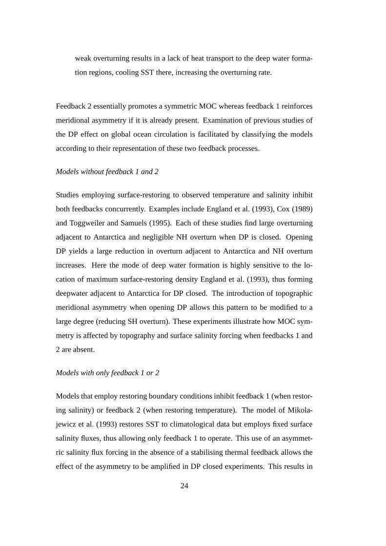
Feedback 2 essentially promotes a symmetric MOC whereas feedback 1 reinforces
meridional asymmetry if it is already present. Examination of previous studies of
the DP effect on global ocean circulation is facilitated by classifying the models
according to their representation of these two feedback processes.
Models without feedback 1 and 2
Studies employing surface-restoring to observed temperature and salinity inhibit
both feedbacks concurrently. Examples include England et al. (1993), Cox (1989)
and Toggweiler and Samuels (1995). Each of these studies find large overturning
adjacent to Antarctica and negligible NH overturn when DP is closed. Opening
DP yields a large reduction in overturn adjacent to Antarctica and NH overturn
increases. Here the mode of deep water formation is highly sensitive to the lo-
cation of maximum surface-restoring density England et al. (1993), thus forming
deepwater adjacent to Antarctica for DP closed. The introduction of topographic
meridional asymmetry when opening DP allows this pattern to be modified to a
large degree (reducing SH overturn). These experiments illustrate how MOC sym-
metry is affected by topography and surface salinity forcing when feedbacks 1 and
2 are absent.
Models with only feedback 1 or 2
Models that employ restoring boundary conditions inhibit feedback 1 (when restor-
ing salinity) or feedback 2 (when restoring temperature). The model of Mikola-
jewicz et al. (1993) restores SST to climatological data but employs fixed surface
salinity fluxes, thus allowing only feedback 1 to operate. This use of an asymmet-
ric salinity flux forcing in the absence of a stabilising thermal feedback allows the
effect of the asymmetry to be amplified in DP closed experiments. This results in
24

large SH overturn (90-100 Sv) which shuts down NH overturn.
Alternatively, models with an energy balance atmosphere and restoring salinity con-
ditions, such as that of Nong et al. (2000) inhibit the positive salt feedback whilst
allowing the thermal feedback. Nong et. al. found large overturning around Antarc-
tica, but also NH overturn for DP closed, in stark contrast to our study. MOC asym-
metry is suppressed as their model allows no positive salt feedback. In addition,
restoring to present day NH surface salinities forces NH overturn to co-exist with a
vigorous SH overturn when the DP is closed. This result is most likely an artifact
of their neglect of a free response of surface salinities to changes in oceanic salinity
transport.
Models with both feedback 1 and 2
Our study and Toggweiler and Bjornsson (2000) are examples where both feed-
backs operate. In the case of Toggweiler and Bjornsson (2000), a meridionally
symmetric fixed FW flux field is employed, resulting in a meridionally symmetric
MOC for DP closed. By also employing an idealised meridionally symmetric to-
pography, Toggweiler and Bjornsson (2000) focuses on the asymmetry introduced
to the MOC by the inhibition of SH overturn upon opening the DP gap. In the
model we use, salinity forcing is not prescribed and a meridional asymmetry devel-
ops as sea-ice production around Antarctica and wind-driven advection of sea-ice
away from the production regions causes a significant wintertime salinity flux into
the ocean through brine-rejection in these areas (figure not shown).
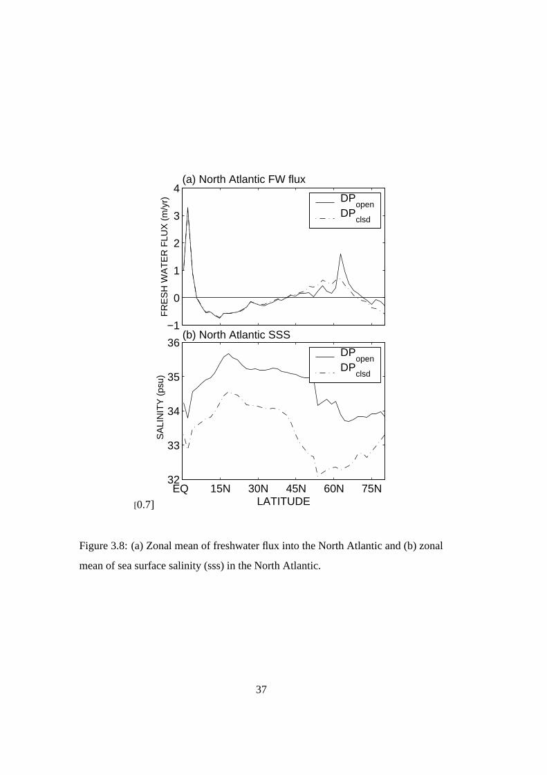
It is of interest to diagnose the relative roles of surface FW fluxes versus oceanic
salt transport in controlling MOC in the North Atlantic in our model experiments.
Figure 8 shows the North Atlantic zonal mean of FW flux into the ocean and the cor-
responding zonal mean of sea surface salinity in in experiments DPclsd and DPopen.
We find that the North Atlantic becomes much saltier upon opening the DP whereas
surface salinity flux changes are small and are mainly driven by the southward dis-
25

placement of the sea-ice edge, representing a redistribution of the FW fluxes due to
sea-ice melt. Therefore, in our study, the sea surface salinity changes in the NH are
not the result of changes in FW forcing across the sea-surface, but are caused by
changes in oceanic salt transport, indicating a weak feedback between oceanic cir-
culation and the atmospheric hydrological cycle (also found in Saenko et al. (2002)
and Hughes and Weaver (1994)).
The positive salt feedback is therefore an important driver for salinity distribution
changes in the model. Our pattern of salinity change in the North Atlantic in DPclsd
is characteristic of that associated with NADW ”collapse”. For instance, Manabe
and Stouffer (1988) and Rahmstorf (1996) find similar salinity differences in the
Atlantic due to a change between the ”on” and ”off” state of NADW formation,
ascribing this to changes in oceanic salt transport. Studies that suppress the sur-
face salinity response to such changes miss important physics in the earth’s climate
system. It is interesting to note that Bryan et al. (1988) find SH overturn of compa-
rable magnitude (55 Sv) to our study and no NH overturn when DP is closed. As in
our model, they employ no restoring conditions for temperature and salinity, thus
allowing both feedbacks 1 and 2 to operate.
The coupled model positive salt feedback and the self-stabilising thermal feedback
are the primary reasons for differences between our study and uncoupled models
such as Nong et al. (2000). However, the wind feedback introduces small modifi-
cations as well, particularly in the SH. Comparing our DPclsd results with the same
run but with the wind feedback suppressed, we find that the East Wind Drift is re-
duced by approximately 10 Sv in the Weddell Sea and the Brazil Current is 4 Sv
weaker in the wind feedback experiment. In contrast, the wind feedback does not
have a significant effect on NH circulation (differenced stream function values are
less than 2 Sv). This implies that the 20 Sv increase in Gulf Stream transport when
DP is opened is almost exclusively the result of thermohaline effects. Although
the wind feedback is an important component of the model, the thermal- and salt
26

feedback effects dominate in our experiments.
3.8. Discussion and Conclusions
Our model results show how significant large-scale cooling of the Southern Hemi-
sphere occurs when the Southern Ocean gateway is opened. The cooling is pri-
marily driven by decreased poleward heat transport to the south, increased sea-ice
extent, and a subsequent increase in the sea-ice albedo. This is contrasted by a
warming in the Northern Hemisphere caused by NADW formation in the DPopen
experiment, a process absent in the DPclsd and DP690 experiments. The described
changes when opening and deepening DP are summarised in a schematic in Figure
9.
One of the key findings of our climate model study is that the Southern Hemisphere
climate in DP690 is similar to that of DPopen, whereas the Northern Hemisphere cli-
mate in DP690 is similar to that of DPclsd. This is because NADW is only initiated
once the DP sill is sufficiently deep, whereas AABW production reduces substan-
tially once a shallow DP gateway is established. This suggests that any change in
southern climate might have occurred rather abruptly upon DP opening during the
Oligocene period, whereas a northern climate response was delayed until a deep
gateway was formed.
The maximum of 15◦C SAT cooling in May-July is observed in the area between
the Ross Sea and the Antarctic Peninsula. The maximum SAT difference is not lo-
cated in this area during summer. Instead, it is located in the South Atlantic Brazil
Current region near 50◦S, showing a 6◦C cooling. Importantly, the fact that the 15
◦C maximum area of SAT cooling is virtually absent in summer suggests a win-
tertime process, such as sea-ice formation, is fundamentally different between the
DPclsd and DPopen experiments. This is confirmed in our sea-ice analysis of section
27

4. Indeed, the wintertime surface air temperature difference maximum occurs in
an area that is ice-covered during winter in the DPopen experiment, but is ice-free
year-round in the DPclsd experiment. Warming in the Southern Hemisphere upon
opening DP occurs south of Australia. SAT warming in this area is also seasonal
due to increased sea-ice frequency in the region.
It should be noted that the versions of the three main experiments presented here
were rerun using the Gent and McWilliams (1990) eddy advection scheme. The
GM experiments yield similar results to those presented here. This suggests that
our findings are robust with respect to the choice of lateral eddy parametrisation.
SST differences between the model experiments are significantly smaller than SAT
changes. This is because of the large capacity of seawater to store and release
heat, which diminishes the sensitivity of SST to model geometry compared to that
of SAT. Northward oceanic heat transport increases in both hemispheres for the
DPopen experiment, reflecting both the onset of NADW formation and the lack of
any significant geostrophic flow across the DP latitudes when an open gateway
exists.
Southern Ocean sea-ice extent for the DPopen experiment is significantly more than
in the DPclsd experiment except for the region north west of the Ross Sea. It is
the year-round absence of sea-ice for DPclsd in the regions west of the Antarctic
Peninsula that causes the SAT differences to be largest (up to 15 ◦C cooling in
DPopen during winter). This is due to the insulating effect of ice and the resulting
decrease in ocean-atmosphere heat loss when opening DP.
The SAT cooling across experiments is smallest in summer, although it is still sig-
nificant (up to 4 ◦C regionally). Summer temperatures are critical for determining
whether an ice cap can build up on Antarctica, as the amount of snow and ice that
survives the summer drives the build-up process, regardless of winter temperatures.
Our results suggest that changes in ocean currents due to the opening of DP may
have helped contribute to the glaciation of Antarctica.
28

Table 3.1: Maximum MOT in the Northern and Southern Hemisphere for DPclsd,
DP690, DP1386 and DPopen measured by the maximum value of the zonally averaged
streamfunction at latitudes of deepwater formation. Mass transport for the Antartic
Circumpolar Current, the Brazil Current and the Gulf Stream are also displayed.
Experiment SH MOT NH MOT ACC Brazil C. Gulf Str.
DPclsd 57 Sv 4 Sv - 66 Sv 24 Sv
DP690 39 Sv 5 Sv 64 Sv 47 Sv 24 Sv
DP1386 21 Sv 6 Sv 121 Sv 25 Sv 24 Sv
DPopen 14 Sv 21 Sv 127 Sv 21 Sv 44 Sv
Table 3.2: Minima of temporal means of zonal mean SAT differences upon open-
ing Drake Passage for DP690 and DPopen. Time periods included are: entire year,
January-March and July-September. Values are in ◦C.
Experiment Year Avg. Jan-Mar Avg. Jul-Sept Avg.
DP690 - DPclsd -2.3 -1.6 -3.3
DPopen - DPclsd -3.7 -2.4 -5.3
29

5
4
3
2
1
DE
PT
H (
km)
(a) Global DPclsd
−55−40
−35−30
−25
−20−15−10−5
−155−25 0
0
5
4
3
2
1
DE
PT
H (
km)
(c) Global DP690
50
−5
−10
−15
−20
−25
−35
−25 −20−105
20
300
−5
90S 60S 30S EQ 30N 60N 90N
5
4
3
2
1
LATITUDE
DE
PT
H (
km)
(e) Global DPopen
20151050−5−10
−5
1510
5
−5
2520 −15
−10−
10
−5
0
0
−15
(b) Atlantic DPclsd
−10
−8 −6 −4 −20
−2
(d) Atlantic DP690
0−2−4−6−
8
−4
30S EQ 30N 60N 90N
LATITUDE
(f) Atlantic DPopen
181614121086420−2−4 −4
−2
10860
Figure 3.1: Global resp. Atlantic Meridional overturning streamfunction (year av-
erage) in Sverdrup (Sv) for (a) resp. (b) the DPclsd case, (c) resp. (d) for the DP690
case and (e) resp. (f) the DPopen case. Values are given in Sv (1 Sv = 106 m3 sec−1).
30

5
4
3
2
1
DE
PT
H (
km)
(a) DP690
− DPclsd
1.5
1
0.5
0.50
0.5
00
−0.
5
−0.5 10.5
0
−0.5
0.5
90S 60S 30S EQ 30N 60N 90N
5
4
3
2
1
LATITUDE
DE
PT
H (
km)
(b) DPopen
− DPclsd
2 2 2.5
1.5
1
0.50−
0.5−
0.5
0
−0.5
−1 −1.50
11
−1.5−
1 −0.5
−0.
5
0
00.5
−1
−2
Figure 3.2: Zonal mean of ocean temperature difference (year average) in ◦C for
(a) DPopen-DPclsd and (b) DP690-DPclsd. Shaded areas denote regions of negative
temperature differences.
31

90S
60S
30S
EQ
30N
60N
90N
LAT
ITU
DE
(a) DPclsd
−60−50−30010
0 10
−80−3020
−50
−40−
30
−20−10
0
0102030
−10
−20−10−30
−40
−50−70
100
6050 20 10
01020
60E 120E 180 120W 60W 0 60E
90S
60S
30S
EQ
30N
60N
90N
LONGITUDE
LAT
ITU
DE
(c) DPopen
30 2010
−10
30 2010
0
0−10
−20−10
−60
−40−30 −40
−30 −20−10 −10
−60030
90110130120
120 10060
10
0
0
(b) DP690
30 2010 20 100
0−10−20−30−40 −70
−40
−30 −20−10
−30
0−10−20
−20−10
−70
−50
−40−30
−20−103060 60 60 7050
−70−3004070
60E 120E 180 120W 60W 0 60E
LONGITUDE
(d) DPopen
− DPclsd
15
105
−10
5
1015406060120 120
1201059060
5
520
90
120
Figure 3.3: Year average of the ocean barotropic streamfunction for (a) DPclsd, (b)
DP690 and (c) DPopen experiments and (d) the barotropic streamfunction difference
for DPopen-DPclsd. Values are given in Sv (1 Sv = 106 m3 sec−1).
32

90S
60S
30S
EQ
30N
60N
90N
LAT
ITU
DE
(a) DP690
− DPclsd
24 cm/s
−10 −6 −2 2 6 10
60E 120E 180 120W 60W 0 60E
90S
60S
30S
EQ
30N
60N
90N(b) DP
open − DP
clsd
19 cm/s
LAT
ITU
DE
LONGITUDE
Figure 3.4: Year average of sea surface temperature difference (25m depth). Values
are in ◦C. Overlayed are vectors of ocean current differences at the surface. A vector
scale is included.
33

90S 60S 30S EQ 30N 60N 90N
−2
−1.5
−1
−0.5
0
0.5
1
NO
RT
HW
AR
D H
EA
T T
RA
NS
PO
RT
(P
W)
LATITUDE
DPclsd
DP690
DPopen
Figure 3.5: Northward oceanic heat transport in DPclsd, DP690 and DPopen.
34

(a) DPclsd
LAT
ITU
DE
90N
60N
30N
EQ
30S
60S
90S
0 0.2 0.4 0.6 0.8 1
(c) DPopen
LONGITUDE
LAT
ITU
DE
60E 120E 180 120W 60W 0 60E
90N
60N
30N
EQ
30S
60S
90S
(b) DP690
− DPclsd
−1 −0.6 −0.2 0.2 0.6 1
(d) DPopen
− DPclsd
LONGITUDE60E 120E 180 120W 60W 0 60E
Figure 3.6: Annual mean sea-ice frequencies for (a) DPclsd, (b) DP690-DPclsd (dif-
ference), (c) DPopen and (d) DPopen-DPclsd (difference).
35

90S
60S
30S
EQ
30N
60N
90N
LAT
ITU
DE
(a) DP690
− DPclsd
−2
−2
−1
−1
0
0
0 −3 −3
1
1
−4
−4
−5
−5
2
−63 −7 −64 −8
1
(b) DPopen
− DPclsd
−3
−3
−2
−2−2
−1
−1
0
0
0
1
1
2
2
−4
−4
1
1
−5
−5
3
3
22
4
−6
5
−7−6
−8
6
3
3
1
−9
−7
4
60E 120E 180 120W 60W 0 60E 90S
60S
30S
EQ
30N
60N
90N
LONGITUDE
(c) DPopen
− DPclsd
(DJF)
−1
−1
0
0
0
1
1 2
2
−2
−2
3
−3
−3
11
4
−4
5
2 −5
6 7 8
3
−6
−1
9
60E 120E 180 120W 60W 0 60E LONGITUDE
(d) DPopen
− DPclsd
(MJJ)
−4
−4
−3−3
−3
−2
−2
−1
−1
0
0
0
1
1
−5−5
−5
−6−6
−6
1
1
2
22
−7
3
−7−8−9
31
−104
−11
−8
−12
5
−13−146 −9
4
−15
1
7−84
8
LAT
ITU
DE
Figure 3.7: Annual surface air temperature difference for (a) DP690-DPclsd and
(b) DPopen-DPclsd. Values are in ◦C. Seasonal surface air temperature differences
DPopen-DPclsd for (c) December-February and (d) May-July. Values are in ◦C.
36
[0.7]
−1
0
1
2
3
4
FR
ES
H W
AT
ER
FLU
X (
m/y
r)
(a) North Atlantic FW flux
EQ 15N 30N 45N 60N 75N32
33
34
35
36
LATITUDE
SA
LIN
ITY
(ps
u)
(b) North Atlantic SSS
DPopen
DPclsd
DPopen
DPclsd
Figure 3.8: (a) Zonal mean of freshwater flux into the North Atlantic and (b) zonal
mean of sea surface salinity (sss) in the North Atlantic.
37

(b) DP at 690m
(a) DP closed
South
Tair warms
PHT
0.6 PWPHT
2.3 PW
PHT
0.7 PW
PHT
2.1 PW
No NADW
cell
Reduced
ice extentPHT
1.2 PWPHT
1.8 PW
NADW outflow
20 Sv ACC 127 Sv
14 Sv
AABW
Ice growth
W arm Tair
North
South North
South North
Tair cools
Further Tair cooling
Ocean
heat
loss
57 Sv
AABW
No NADW
cell
ACC
64 Sv
39 Sv
AABW
Sea-ice
Sea-ice
(c) DP open
Figure 3.9: Schematic representation of the major ocean circulation, heat transport,
ice and air temperature features of the three experiments.
38

Chapter 4
Transient behaviour: the role of
Drake Passage in controlling the
stability of the ocean’s thermohaline
circulation
4.1. Abstract
We examine the role of a Southern Ocean gateway in permitting multiple equilib-
ria of the global ocean thermohaline circulation. In particular, necessary condi-
tions for the existence of the multiple equilibria are studied with a coupled climate
model, wherein stable solutions are obtained for a range of bathymetries with vary-
ing Drake Passage (DP) depth. We find no transitions to a Northern Hemisphere
overturning state when the Drake Passage sill is shallower than a critical depth
(1100m in our model). This preference for Southern Hemisphere sinking is a result
of the particularly cold conditions of the Antarctic Bottom Water (AABW) forma-
39

tion regions compared to the NH deepwater formation zones. In a shallow or closed
DP configuration, this forces an exclusive production of deep/ bottom water in the
Southern Hemisphere. Increasing the depth of the Drake Passage sill causes a grad-
ual vertical decoupling in Atlantic circulation, removing the influence of AABW
from the upper 2000m of the Atlantic ocean. When the DP is sufficiently deep,
this shifts the interaction between a North Atlantic Deep Water (NADW) cell and
an AABW cell to an interaction between a (shallower) Antarctic Intermediate Wa-
ter cell and a NADW cell. This latter situation allows transitions to a Northern
Hemisphere overturning state.
4.2. Introduction
The gradual deepening of a Southern Gateway since the Oligocene is thought to
have had an influence on Antarctic climate (Kennett 1977). Toggweiler and Bjorns-
son (2000) and Sijp and England (2004, hereafter SE2004) use climate models to
suggest that Southern Hemisphere (SH) climate change due to the opening of a
Drake Passage (DP) is relatively abrupt, in that it occurs once even a shallow DP
is established. They based this conclusion on findings that the SH climate for a
shallow DP experiment is very similar to that of today, yet markedly different to the
DP closed climate. The DP closed (DPclsd) experiment in SE2004 exhibits large
SH overturning and no NADW formation. Southern Hemisphere sinking is particu-
larly vigorous in the DPclsd experiment, where 55 Sv sink off Antarctica. However,
no attempts were made in either SE2004 or Toggweiler and Bjornsson (2000) to
excite transitions to a possible Northern Hemisphere (NH) overturning state. Here
we examine the existence of multiple equilibria for a range of DP depths, including
closed, in a coupled climate model.
Bryan (1986) showed that stable interhemispheric overturning states with predomi-
nant sinking in one hemisphere can be obtained in a rectangular basin geometry un-
40

der symmetric surface forcing. The density contrast between the antipodean deep-
water formation regions determines the strength and polarity of this circulation. For
example, a SH sinking state corresponds to higher SH surface densities. However,
a striking simplification of Bryan’s geometry is the absence of a circumpolar ocean
at the latitudes of the DP. In the real ocean, this unbounded region constitutes an
obstruction to meridional geostrophic flow to higher southern latitudes (Toggweiler
and Samuels 1995). As a result of the DP gap, ocean ventilation of Antarctic Inter-
mediate Water (AAIW) occurs to depths of around 1000m (e.g. Cox 1989). Saenko
et al. (2003) demonstrate the importance of the relationship between densities in
the AAIW formation regions (ρAAIW ) and those in the North Atlantic Deep Water
(NADW) formation regions (ρNADW ) in determining the global ocean Meridional
Overturning (MOC). For example, a SH sinking state is found when freshwater
(FW) is extracted from the AAIW formation regions such that ρAAIW> ρNADW .
Unlike Bryan (1986) and the DP closed case of SE2004, this SH state consists of an
AAIW reverse cell overlying a circulation of Antarctic Bottom Water (AABW) in
the Atlantic below 2000 m depth. The AAIW reverse cell favours an enhanced FW
flux into the Atlantic, transporting relatively saline low-latitude waters out of the
Atlantic near the surface whilst importing fresher AAIW. Saenko et al. (2003) show
that the resulting freshening of the North Atlantic (NA) prevents ρNADW from ris-
ing above ρAAIW after cessation of the FW extraction, thus yielding a stable NADW
‘off’ state.
Whilst it is clear that the ocean is characterised by an interhemispheric competi-
tion for ventilation dominance, the role of SH-NH land-mass asymmetry in setting
stable climate equilibria remains relatively unexplored. In this study we examine
the role of the depth of the DP sill in permitting multiple equilibria in the ocean’s
thermohaline circulation (THC). It will be shown that the depth of the DP sill plays
a fundamental role in determining the relative importance of the three global wa-
ter masses (AABW, AAIW and NADW) in setting the global ocean THC. AABW
mostly forms in the Ross and Weddell Seas, spreading below NADW, whereas in-
41

tensive AAIW formation is thought to occur in a localized region around the tip
of South America (McCartney 1977; England et al. 1993). A schematic of these
formation regions is indicated in Figure 4.1. We will show that the dominant SH
water-mass formation site shifts gradually from AABW to AAIW with deepening
DP, thus shifting the thermohaline circulation control from ρNADW vs. ρAABW
(DPclsd) to ρNADW vs. ρAAIW (DPopen). Different surface density conditions in
these respective areas make the latter density contrast more favourable to a NADW
‘on’ state, as seen in today’s climate.
4.3. Methodology
The simulations have been carried out using the Earth System Climate Model of
intermediate complexity of Weaver et al. (2001) described in Chapter 2. Here, we
use version 2.5. To model the effect of unresolved meso-scale eddies, we employ
constant horizontal diffusivity of 2.0 × 107 cm2 s−1. Vertical mixing is achieved
through a modified form of the Bryan and Lewis (1979) vertical distribution, rang-
ing from kv=0.6 cm2 s−1 in the upper ocean to kv=1.6 cm2s−1 in the deep ocean.
No wind feedback is used.
Our experiments are based on 2100 year integrations from idealized initial condi-
tions in six bathymetries, set up identically with the exception of the DP sill depth.
Table 1 lists the DP sill depths considered in this study, ranging from 0 (DPclsd)
down to 2316m (DPopen). We then apply FW perturbations to these experiments in
order to obtain states with no NADW formation, and if possible, states with NADW
formation. All experiments can be perturbed to yield a state with no NADW forma-
tion. This state is denoted by NADWoff . Some experiments exhibit a steady-state
with NADW overturn, these are denoted by NADWon. We denote the FW pertur-
bations by Forcing 1 and Forcing 2 (shown in Figure 4.6b). These perturbations
involve the addition of an extra term to the usual surface salinity flux field other-
42

wise determined by internal model factors such as precipitation, evaporation, sea-
ice growth/ melt, river runoff and runoff outside river mouths. This artificial FW
loss is applied uniformly inside the grey and red regions shown in Figure 4.1. The
two forcings vary to simulate pulses of FW extraction from the North Atlantic to
excite possible transitions to stable NADW formation states. Forcing 1 consists of
a linear decrease from zero to -2.25 mm/day at year 150, returning to zero pertur-
bation by year 300. This is equivalent to an integrated North Atlantic FW loss of
0.7 Sv at the peak of the freshwater anomaly. Forcing 2 is double the intensity of
Forcing 1.
We use identical seasonal wind stress fields throughout the experiments. We thus
do not examine the effect of a varying wind stress in driving the NH overturning.
The so-called ”Drake Passage effect” -where winds over the Southern Ocean con-
trol, in part, the rate of NADW production- has been examined in many studies (e.g.
Toggweiler and Samuels 1995; Rahmstorf and England 1997; Tsujino and Sugino-
hara 1999; Klinger and Drijfhout 2004). There is still some debate as to whether this
control is via mechanical (Toggweiler and Samuels, 1995) or wind-driven buoyancy
effects (Gnanadesikan and Hallberg 2000). It is noted that the DP effect requires a
DP sill depth of ∼1500-2000m, much deeper than our shallow DP experiments. In
addition, with fixed seasonal wind stress forcing in our experiments, the DP-effect
is beyond the scope of this study. We will explain model MOC behaviour in terms
of buoyancy effects, a natural consequence of the buoyancy perturbations employed
in our experimental design.
4.4. Overturning diagnostics
To study the dynamic behaviour of the Atlantic MOC in response to the FW pertur-
bations, we record the NADW formation rate as the maximum value of the MOC in
the downwelling branch of the North Atlantic (see Figure 4.7). We also record the
43

following MOC quantities:
1. Atlantic AAIW reverse cell strength: In the NADWoff states of all experiments
except DPclsd the AAIW reverse cell and the AABW cell are separated by a local
minimum of the absolute strength of the MOC, occurring at around 2000 m depth
(see Figure 4.5b-f). We measure the strength of the AAIW reverse cell by tak-
ing the difference between this absolute minimum and the peak magnitude of the
AAIW cell at 30 ◦S (usually occurring in the upper 1000m if a reverse cell exists).
Figure 4.5b-f indicates this cell strength.
2. NADW outflow: This is taken to be the maximum of the MOC in the Atlantic
sector at 33◦S (see Figure 4.7), normally occurring at around 1600 m depth.
3. Atlantic AABW inflow: This is taken as the maximum magnitude of the abyssal
MOC cell at 33◦S in the Atlantic sector. This measures the amount of inflow of
AABW into the Atlantic (see Figure 4.5).
4. Atlantic AABW upwelling: This is taken to be the magnitude of upwelling trans-
port across 1980 m depth in the Atlantic sector between 33◦S and 59◦N (see Fig-
ure 4.5). This measures the net amount of water upwelled across 2000 m depth in
the Atlantic.
4.5. Results
a. NADWoff states
We begin by analyzing the equilibrium overturning of the respective NADWoff
states. Figure 4.2 shows the global MOC for DPclsd, DP690 and the NADWoff state
of DPopen taken from 10 year means at the end of the unperturbed model integra-
tions. DPclsd exhibits a large interhemispheric overturning cell (55 Sv) originating
44

in the SH. When the DP is opened to 690 m depth, with still no NADW formation, a
dramatic change in MOC occurs in the SH: the Deacon Cell appears1, characterised
by surface Ekman transport balanced by a deeper return flow beneath the DP sill,
and the AABW production rate drops from 55 Sv to only 35 Sv. This reduction in
AABW is independent of any interhemispheric density forcing, and entirely due to
the emergence of a DP gap. The DPopen case shows that further deepening of DP
results in a deeper Deacon Cell and a further reduction of the AABW cell down to
its pre-industrial value of ∼15 Sv (Broecker et al. 1999).
In order to examine the relative roles of temperature and salinity in determining the
vigorous sinking of AABW in the DP closed case, we have run experiments where
salinity is held constant at 34.72 psu. We denote these versions of the DP exper-
iments with Soff . The MOC solutions obtained for these experiments are unique
as multiple equilibria do not occur in the absence of salinity effects. Indeed, Stom-
mel (1961)’s box model exhibits a thermally driven solution and a salinity-driven
solution. The Soff experiments yield an AABW overturning of around 60 Sv (fig-
ure not shown) for DPclsd Soff , indicating that the large SH overturning cell in the
standard DPclsd experiment where salinity is an interactive component is thermally-
driven and no significant overturning strength is derived from the positive salt feed-
back. Figure 4.3 shows the Atlantic Meridional overturning streamfunction for the
Soff experiments in bathymetries: (a) DPclsd, (b) DP690, (c) DP896, (d) DP1128, (e)
DP1386 and (f) DPopen. Similar to the standard experiment DPclsd, a strong inter-
hemispheric AABW penetrates the Atlantic with approximately 12 Sv upwelling
across 2000m depth in DPclsd Soff (Figure 4.3 a). In contrast to the standard ex-
periment DPclsd, a weak NH cell of around 8 Sv recirculates inside the North At-
lantic. This cell occurs because, unlike in the standard experiment, no positive salt
feedback is present to fully shut down NH overturning. Due to the colder AABW
formation regions (compared to the NADW formation regions) we find that the SH
1It is noted that the Deacon Cell mostly disappears in density coordinates (Doos and Webb 1994)
and so does not play a major role in water-mass modification in the Southern Ocean.
45

cell is much stronger than the NH cell in our experiments. This is in agreement with
our DPclsd result where salinity is interactive. The MOC of the Soff experiments
can be interpreted as a measure of the thermal driving available to the MOC due to
meridional thermal gradients at the surface in the standard experiments where salin-
ity is interactive. Under symmetrical thermal surface conditions (about the equator)
at the deepwater formation regions, we expect a symmetrical overturning in the
DPclsd Soff experiment akin to the symmetrical state found by Bryan (1987). Due
to the colder conditions around Antarctica, however, we find a modification of this
symmetrical pattern with a strong weighting towards SH overturn. When salinity is
interactive, the positive salt feedback comes into action and reinforces the southern
or northern cell at the expense of the antipodean cell. The symmetrical forcing and
topography of Bryan (1987)’s model also allow a stable symmetrical MOC state ex-
hibiting a northern and southern cell of equal strength. A small salinity perturbation
in either hemisphere allows the positive salt feedback to reinforce sinking in that lat-
itude, culminating in a large interhemispheric cell and precluding overturning in the
opposite hemisphere. We see from Figure 4.3 that thermal driving in our model is
not symmetrical, and we will see later that the positive salt feedback is unable to
supplement the weak thermal driving available to the NH cell sufficiently to yield a
stable NH overturning state. Upon the introduction of a shallow DP gap (Figure 4.3
b), however, we find a significant strengthening of the NADW recirculation inside
the Atlantic to 12 Sv. This indicates a significant increase in thermal driving avail-
able to the NH cell. AABW inflow into the Atlantic is reduced to 4 Sv, and AABW
upwelling there is reduced to 2 Sv. This trend continues with deepening DP until
AABW no longer upwells across 2000m depth and 2 Sv of NADW outflow appears
in DP1128 Soff (d). Further deepening of DP (e, f) results in stronger formation and
outflow of NADW. AABW circulation remains very similar once NADW outflow
is established (d, e and f). As in the standard experiments, AABW inflow is 4 Sv
once a DP is established in the Soff experiments. The 16 sv of NADW formation
in DPopen Soff (f) indicates that the 18 Sv of NADW formation in the standard
experiment is largely thermally driven, and some amplification occurs by way of
46

the positive salt feedback when salinity is an interactive field, resulting in a 2 Sv
increase in NADW sinking. It is interesting to note that the most shallow DP depth
(1128 m) at which NADW outflow occurs in the Soff experiments is also the most
shallow depth at which we find multiple equilibria in the standard experiments. It
is not clear whether this is a coincidence.
Figure 4.5 shows the Atlantic MOC for the NADWoff states for each of the DP
bathymetry experiments taken from 10 year means. Figure 4.5 (a) shows that in
DPclsd the SH AABW cell extends to the high northern latitudes and dominates
all depth levels of the Atlantic. A second water-mass (AAIW) appears when a
shallow (690m) DP gap is introduced (Figure 4.5b). Waters in the upper 2000m
of the Atlantic now originate from AABW upwelling across 2000m (5.6 Sv) and
AAIW flowing across 30◦S (5 Sv). The AAIW component forms a reverse cell,
enveloped by a larger AABW cell. Figures 4.5 (b)-(f) show that with a deepening
DP the dominant ventilation in the upper 2000m of the Atlantic shifts gradually
from AABW upwelling to AAIW inflow. Note also the gradual vertical partitioning
across 2000m in the Atlantic MOC as DP deepens: two vertically stacked SH cells
emerge (DPopen) from one SH AABW cell (DPclsd). Another interesting feature
of Figure 4.5 is that once a shallow DP gap is established, AABW inflow remains
relatively constant (around 5 Sv, see Table 4.1) even as DP is deepened.
Figure 4.4 shows the zonal mean of sea surface salinity (sss) in the Atlantic for
DPopen, DPopen NONADW and DPclsd. It may be noted that North Atlantic fresh-
water fluxes (3.8) are reasonably similar for both the NADWoff and the NADWon
states in DPopen. Yet we see from Figure 4.4 and later sections that sea surface salin-
ity is substantially different between NADWon and NADWoff states, regardless of
DP batyhmetry. This indicates that surface circulation, not FW fluxes, determines
sea surface salinity (SSS) to a large extent in the North Atlantic. Furthermore, the
similarity of the zonally averaged Atlantic SSS field for DPopen NONADW and
DPclsd suggest that Atlantic SSS is determined by MOC polarity rather than the na-
47

ture of the SH cell. The North Atlantic horizontal circulation field is very similar
for the NADWoff case in DPopen and the steady state (ie. NADWoff ) field in DPclsd
(Figure not shown). In fact, all NADWoff cases show a highly similar pattern of
horizontal circulation in the North Atlantic, regardless of DP geometry.
b. Response to FW perturbations
Figure 4.6 shows the transient response of NADW production to the FW pertur-
bations for the six bathymetries. For each bathymetry the NADWoff state is used
as the initial condition. The time-series shown in Figure 4.6 (a) corresponds to
the NADW production for DPopen, DP1386 and DP1128 under Forcing 1 and DPclsd,
DP690 and DP896 under Forcing 2. The time-series show a successful transition to
a NADWon state for DPopen, DP1386 and DP1128 under the moderate FW pertur-
bation of Forcing 1. In contrast, we fail to obtain stable NADWon states for the
remaining bathymetries DPclsd, DP690 and DP896 under the stronger FW extraction
of Forcing 2. We have also subjected these experiments to an even stronger and
more prolonged forcing (figure not shown) applied concurrently with opposite sign
in each hemisphere. Although AABW is fully suppressed for a prolonged period
of time in these experiments, the MOC returns to a SH polarity after removal of
the FW forcing, with no sustenance of NADW. Finally, we note the relatively slow
decay of NADW in DP896. There appears to be a threshold depth of the DP sill
above which NADW cannot be sustained. The DP896 case would appear to lie close
to this threshold in our model.
It is worth briefly discussing the NA MOC obtained for the NADWon states. Fig-
ure 4.7 shows the Atlantic MOC for (a) DP1128 and (b) DPopen in the NADWon
states. Although DP1128 exhibits less NADW formation and outflow compared to
DPopen, there is a general similarity in overturning patterns between the two exper-
iments. NADW formation and outflow are reduced in DP1128 by ∼2 Sv and ∼4
48

Sv, respectively, compared to DPopen. This reduction in NADW outflow will be
shown to be consistent with a reduction in northward branching of AAIW as DP
progressively deepens (see section 4.6). By conservation of mass, reduced AAIW
northward flow must result in reduced NADW outflow.
Figure 4.8 shows several other MOC quantities in DPclsd and DP1128 measured dur-
ing the model response to Forcing 2 designed to excite a transition from a NADWoff
state to a NADWon state. Unlike DP690, DP1128 exhibits a transition to a stable
NADWon state. During sustenance of NADW, DP1128 shows a collapsed AAIW re-
verse cell (Figure 4.8c), no AABW upwelling across 2000 m depth in the Atlantic
sector (Figure 4.8d), and a steady AABW inflow of ∼4 Sv (Figure 4.8e). In con-
trast, NADW cannot be sustained in DP690. Immediately after the end of the FW
extraction period AABW inflow starts to recover to its previous value of >5 Sv.
Several hundred years later, AABW upwelling across 2000m is re-established, as is
the AAIW reverse cell. By this time, NADW is nearing its final collapse and return
to a steady NADWoff state.
Figure 4.9 shows the temperature and salinity properties at the sea surface in the
NADW, AABW and AAIW sinking regions for the nine different equilibria. NADWon
states are shown for DPopen, DP1386 and DP1128, and the NADWoff states are shown
for all bathymetries from DPopen to DPclsd. The colours correspond to the water-
mass formation regions shown in Figure 4.1. The variation of ρAABW (blue) is rel-
atively small among the equilibria, as it is for ρAAIW (green). However, for ρNADW
(red) there are two distinct clusters of points. One cluster is characterised by T-S
of ∼5.5◦C and 34.9 psu, with density lying between 1027.5 and 1027.6 kg/m3;
this corresponds to the NADWon states. The other cluster is markedly colder and
fresher (0.5◦C and ∼32.6 psu) with a density range of 26.1 to 26.3 kg/m3; this
corresponds to the NADWoff states. Therefore ρNADW > ρAAIW in the NADWon
states and ρNADW < ρAAIW in the NADWoff states. The approximate T-S proper-
ties of an idealized mixture of AAIW and AABW are indicated by the dashed line
49

in Figure 4.9. This line varies between experiments but for clarity only one line
is shown here. NADW is only denser than the mixture of Antarctic water masses
once AAIW dominates this mixture (approximately 75% AAIW, 25% AABW is
required). Our experimental results suggest that a sufficiently deep DP is required
to enable AAIW to dominate from the south. Otherwise, a shallow or closed DP
sees dense AABW inhibiting the excitation of NADWon states, regardless of AAIW
densities.
c. Sensitivity to model experimental design
The critical depth of DP that enables NADW production to be sustained also de-
pends in part on the particular thermal forcing used in the model. In our experi-
ments, heat fluxes between the ocean and atmosphere resemble that of the present-
day climate, resulting in a given set of THC equilibria as described above. However,
if our model is forced using different surface heat fluxes, such as a colder North
Atlantic, a different set of equilibria will emerge. To further assess this we have ex-
amined experiments wherein the southern bias of the thermal asymmetry between
the AABW and NADW formation regions is reduced by applying a permanent heat
extraction of 200 W/m2 in the North Atlantic. This is undertaken in experiments
DPclsd and DP690. New equilibria with only a small drop in global temperature are
obtained as a new radiative balance with space is established. Application of Forc-
ing 2 to this heat-modified version of DP690 yields a transition to a stable NADWon
state (note that this enhanced heat flux experiment also allows a stable NADWoff
state). The DPclsd case, in contrast, does not sustain NADW production under these
modified heat fluxes. Thus, caution should be taken when quantifying the critical
depth for DP to enable excitation to NADWon states, as this critical depth depends
in part on the global air-sea heat fluxes applied in the model. Under present-day
thermal forcing, we have found that a critical DP depth of ∼1000m enables NADW
to be sustained in a steady state.
50

Parametrization of subgrid-scale mixing is another factor that may influence the
critical DP sill depth obtained in the model. We ran a DPclsd experiment employing
the sub-grid scale eddy parametrization of Gent and McWilliams (GM) and found
large rates of AABW formation (∼44 Sv). As in our standard DPclsd experiment,
no stable NH overturning states could be excited in response to perturbations of the
NA. In contrast, a DPopen case with GM mixing permits a NADWon state. This in-
dicates that there must also be a critical DP sill depth that allows NADW formation
to be sustained in experiments using GM. We have not explored a full DP depth
series of experiments to identify this critical depth under GM. The important point
is that such a depth exists, though its exact level will likely vary slightly according
to model configuration.
4.6. Discussion
The North Atlantic freshwater perturbation experiments assessed in this study sug-
gest that a DPclsd geometry cannot sustain a stable NH overturning state under a
present day climate forcing. In DPclsd the polarity and strength of the global MOC
depends on the interhemispheric density contrast between the high latitude deep-
water formation regions (as also noted by Rooth 1982; Bryan 1986). In Bryan’s
study the asymmetric overturning states are stable under symmetric surface forc-
ing since a north-south salinity contrast is maintained by an interhemispheric MOC
cell. In our model, surface thermal forcing is not symmetric: heat loss in the SH
deepwater formation regions is significantly larger than that in the NH due to the
local atmospheric forcing. The cold Antarctic conditions force a large SH sinking
in DPclsd.
Unless a dramatic cooling over the NA is artificially prescribed, none of the FW per-
turbations we employed could excite a transition to a state where ρNADW remains
above ρAABW in a DPclsd geometry. In the present-day climate ρAABW > ρNADW
51

and so NADW formation occurs by virtue of the existence of a deep DP that limits
AABW production and sufficiently restricts the influence of this water mass to lev-
els below 2000 m depth in the Atlantic. With the introduction of a DP gap, a third
water-mass, AAIW, enters the stage. Our results suggest that as DP deepens there is
a gradual shift in importance from ρAABW to ρAAIW in the relation between SH sur-
face density and ρNADW as DP deepens. Figure 4.9 shows that the NADWon states
in the cases that permit multiple equilibria (DP1128, DP1386 and DPopen) are charac-
terised by the relation ρNADW> ρAAIW . Saenko et al. (2003) stress the importance
of this relationship in determining whether stable NADW sinking can occur.
The decreased influence of AABW that upwells above 2000 m depth in the Atlantic
Ocean (Figure 4.5) reveals the mechanism by which the shift in importance from
ρAABW to ρAAIW occurs. When DP is shallow, there is significant upwelling of
AABW to the surface in the Atlantic. This mass transport forms a closed cell that
encompasses the surface layers and the AABW formation regions (Figure 4.2b).
This situation is similar to DPclsd. In the shallow DP experiments (DP690 and DP896)
surface waters downwelled north of the DP gap recirculate to AABW formation re-
gions (Figure 4.2b), thereby sustaining the dominance of AABW on global MOC
polarity. With deepening DP this mechanism of AABW dominance is impaired
by an increasing obstruction for poleward geostrophic flow across the DP gap to
the AABW formation regions. Water downwelled north of the DP exhibits an in-
creasing preference for northward flow (as AAIW) instead of geostrophic flow to
the south. This is because the downwelled water has more difficulty reaching the
depths of the increasingly deep DP sill due to its buoyancy. The NADWoff states
displayed in Figure 4.5 involve a gradual increasing preference (as DP deepens) for
a northward branching of the water downwelled north the circumpolar gap, thus
causing a gradual increase of AAIW inflow. This increase of AAIW inflow comes
at the expense of AABW upwelling across 2000 m depth (Table 4.1). With more or
less constant AABW inflow once DP is opened, AABW increasingly tends to re-
circulate below 2000 m depth as DP deepens (Figure 4.5). The influence of ρAABW
52

in the upper 2000m is thus reduced and it becomes possible for NADW to overly
the Atlantic variety of AABW. With an increasing amount of AAIW inflow, ρAAIW
becomes a key factor in determining interhemispheric MOC patterns. At some
stage a threshold occurs (in our experiments between DP sills at 896m and 1128m)
where the influence of the high ρAABW (due to cold conditions around Antarctica)
becomes sufficiently reduced with respect to the lighter ρAAIW to allow a stable
NADWon state. The observed reduction in NADW outflow for the stable NADWon
states shown in Figure 4.7 with decreased DP depth also results from a decreased
southward branching of water downwelled north of DP.
Global MOC polarity is determined by the sign of (α(D) · ρAABW + β(D) · ρAAIW
- ρNADW ) where D is the DP depth. However, ρAAIW also affects the penetration
depth of AAIW. The fraction of north/ south branching in the bifurcation of water
downwelled north of DP is determined by the DP depth and by the buoyancy of the
downwelled water. Therefore, a change in ρAAIW while D remains constant can
also affect the bifurcation. This means that α and β are functions of ρAAIW as well
as D. We find, however, that ρAAIW remains relatively constant across experiments
with changes in D (see Figure 4.9). This means that the bifurcation rates depend
almost exclusively on the DP depth in our experiments.
We assessed the role of surface heat flux forcing in determining the critical threshold
DP depth for NADW formation to be sustained. Under a present-day heat flux
forcing scenario, this critical DP depth appears to be around 1000m. However,
different heat flux scenarios, such as a cooler NA, see different threshold DP depths.
For example, a sufficiently high ocean heat loss in the NA is found to permit a
stable NADWon state in the DP690 geometry. From a paleoclimate perspective, this
suggests that while the DP depth controls the existence of multiple ocean equilibria,
there is no single threshold depth that characterises all climate states.
Figure 4.10 shows a schematic diagram of the NADWoff and NADWon states with
DP at its present day depth. Note the bifurcation in the downwelling route north
53

of the DP gap in NADWoff . The fraction of mass in each part of the bifurcation
regulates the relative importance of ρAABW and ρAAIW : greater northward branch-
ing (as occurs once DP is deep) shifts the emphasis to ρAAIW . Increasing the DP
depth strengthens the northward branch at the expense of the southward branch in
the bifurcation. The NADWon state is completely different, with no reverse cell of
AAIW, and NADW forming a closed cell that encompasses the Deacon Cell. In
addition, no AABW is upwelled across 2000 m depth in NADWon, even though the
AABW inflow appears relatively unchanged between the NADWoff and NADWon
states.
4.7. Conclusions
We have shown that NADW formation and stability depend critically on the depth
of the DP sill via the interplay between northern and southern water masses. As
DP deepens a greater component of AAIW flows to the north of its formation re-
gion, shifting the AABW-NADW competition in DPclsd to one combining the more
buoyant AAIW mass. This eventually enables NADW to form stably once a critical
DP depth is reached.
Models resolving a net mass transport across the ACC induced by mesoscale eddies
allow an increased shallow southward conduit for water originating north of the DP
gap. Gnanadesikan (1999) refers to this as the ‘Eddy return flow’ in his elegant
model and finds a negative effect on NADW formation through a shoaling of the
pycnocline. By analogy, our results show that an increased southward conduit oc-
curs when DP is shallow; which in turn increases AABW upwelling across 2000m
and strengthens the importance of that water-mass in controlling the global MOC.
Further examination of the effect of the DP gap on global climate could include
systematic variations in the hydrological cycle as well as the thermal conditions
54

in the Northern and Southern Hemispheres, employing varying geometries with
different DP depths. In this note, we have shown that the depth of the DP sill is of
first order importance in controlling the stability of the ocean’s global thermohaline
circulation.
55

Table 4.1: List of all experiments and DP depth (in meters). The third column
indicates whether a NADWon state is found. The last three columns show At-
lantic AABW inflow, AABW upwelling across 2000m depth and the strength of
the AAIW reverse cell in the Atlantic for the NADWoff states (for definitions of
the MOT quantities see section 2.3. All transport values are given in Sv (1 Sv = 106
m3 sec−1).
Expe
rimen
t
DP
Dep
th(m
)
NA
DW
exis
ts?
AA
BW
inflo
w
AA
BW
upw
ellin
g
AA
IWre
vers
ece
ll
DPclsd 0 no 12.5 12.5 -
DP690 690 no 5.3 5.0 5.6
DP896 896 no 5.0 3.4 7.1
DP1128 1128 yes 5.0 2.3 8.6
DP1386 1386 yes 4.9 1.5 9.7
DPopen 2316 yes 4.6 0.8 10.4
56

0 60E 120E 180 120W 60W 90S
60S
30S
EQ
30N
60N
90N
LONGITUDE
LAT
ITU
DE
AAIW
AABWAABW
NADW
density contrast
Drake Passage
Figure 4.1: Model domain and primary water-mass formation regions. The grey and
red areas in the North Atlantic combined indicate the region used in FW extraction
under Forcing 1 and 2. The density contrast between NH and SH sinking regions
determines the structure of the Atlantic MOC. With a deepening DP, the importance
of the AABW formation regions shifts to the AAIW regions. Formation regions for
AABW (blue), AAIW (green) and NADW (red) are also indicated.
57

5
4
3
2
1D
EP
TH
(km
)
(a)DPclsd
−55 −45
−45
−40
−35−
30 −25
−20−15
−10
−5
−20−1000
5
4
3
2
1
DE
PT
H (
km)
(b) DP690
0
5
−5
−10
−15
−20−2
5
−35
−25
−20
−10 −5025
60S 30S EQ 30N 60N5
4
3
2
1
LATITUDE
DE
PT
H (
km)
(c) DPopen
50−5−10
−15
25
15
50
−5 −10
−25−20
−10
−5
0
Figure 4.2: Global meridional overturning streamfunction (10 year average) for the
NADWoff states in bathymetries (a) DPclsd, (b) DP690 and (c) DPopen. Values are
given in Sv (1 Sv = 106 m3 sec−1). The outline of the DP gap is indicated by
shading.
58

5km
4km
3km
2km
1km
DE
PT
H (
km)
(a) MOT Atlantic DPclsd
SOFF
6420−1−2−4−6
−8
−10
−1
−2−1
−1−2−4
−6
5km
4km
3km
2km
1km
DE
PT
H (
km)
(c) MOT Atlantic DPlv7
SOFF
12
1086420−1−2−4
−2−4
−1
−2
30S EQ 30N 60N 90N
5km
4km
3km
2km
1km
LATITUDE
DE
PT
H (
km)
(e) MOT Atlantic DPlv9
SOFF
14
12108
64
20−1−2−4
−4
−2−1
420−2−4
(b) MOT Atlantic DPlv6
SOFF
121086420−1−2
−4
−4−2
−1
(d) MOT Atlantic DPlv8
SOFF
1412108642
0−1−2−4
−4
−2−1
20−1−2
−4
30S EQ 30N 60N 90NLATITUDE
(f) MOT Atlantic DPopen
SOFF
1614121086420−2−4
−4−4−2
−1
20−1
64 20−1−4
Figure 4.3: Atlantic Meridional overturning streamfunction (10 year average) for
the Soff experiments in bathymetries: (a) DPclsd , (b) DPlv6, (c) DPlv7, (d) DPlv8,
(e) DPlv9 and (f) DPopen. Values are given in Sv (1 Sv = 106 m3 sec−1).
59

30S 15S EQ 15N 30N 45N 60N 75N32
32.5
33
33.5
34
34.5
35
35.5
36
36.5
LATITUDE
kg/m
3
(b) Zonal mean of SSS (kg/m3) North Atlantic
DPopen
DPopen
NONADWDP
clsd
Figure 4.4: zonal mean of sea surface salinity (sss) in the Atlantic for DPopen,
DPopen NONADW and DPclsd.
60

5
4
3
2
1
DE
PT
H (
km)
(a) DPclsd
−13−10 −8 −7
−6−5
−4−3
−2
−1
0
5
4
3
2
1
DE
PT
H (
km)
(c) DP896
−9
−8 −7
−6−5 −4−3
−2
−1
−4−3
−1−2
0
30S EQ 30N 60N5
4
3
2
1
LATITUDE
DE
PT
H (
km)
(e) DP1386
−10
−7−6 −5 −4−3−2
−2−3−4
−1
0
30S EQ 30N 60N
LATITUDE
(f) DPopen
−10 −8 −6 −5 −4−3 −2−1−1
−2−3−4
−3−2
−1
0
0
(d) DP1128
−9 −7 −6−5 −4−3
−2−3−4
−2
−1
−2
0
(b) DP690
−8 −7 −5−4 −3 −2
−1
−3−2
−1
−5
0
{
{
{ {
{
AAIW rev . cell :5Sv
AAIW rev . cell: 9 Sv
AAIW rev . cell: 10 Sv
AAIW rev . cell: 10Sv
AAIW rev . cell: 7 Sv
{
{
{ {
{ AABW in− flow: 5 Sv
AABW in− flow: 5Sv
AABW in− flow: 5 Sv
AABW in− flow: 5Sv
AABW in − flow: 5 Sv
~5 Sv upwelling
~2Sv upwelling
<1Sv upwelling~2Sv upwelling
~3 Sv upwelling
{ 13 Sv
−1
−1
Figure 4.5: Atlantic meridional overturning streamfunction (10 year average) for
the NADWoff states in bathymetries (a) DPclsd, (b) DP690, (c) DP896, (d) DP1128,
(e) DP1386 and (f) DPopen. Values are given in Sv (1 Sv = 106 m3 sec−1).
61

0
5
10
15
20
25
30
35(a) NADW production
SV
0 250 500 750 1000 1250 1500 1750 2000 2250 2500
−5
0
5(b) FW perturbation
TIME(years)
FLU
X(m
/yr)
Forcing 1Forcing 2
DPopen
DP1386
DP1128
DP896
DP690
DPclsd
Figure 4.6: (a) NADW production rate vs. time in the series of experiments con-
ducted to excite transitions to NADWon states. (b) Time history of FW perturbations
in Forcings 1 and 2. The timeseries of NADW production in (a) exhibit a success-
ful transition to NADWon states for DP1128 (green), DP1386 (black) and (f) DPopen
(blue) in response to Forcing 1. Even under the stronger Forcing 2 there is no ex-
citation of a transition to a NADWon state for DPclsd (red), DP690 (cyan) and DP896
(yellow). Note that here DPopen, DP1386 and DP1128 are forced with Forcing 1 (blue
in b), whereas DPclsd, DP690 and DP896 are forced with the stronger perturbation of
Forcing 2 (black in b).
62

5
4
3
2
1
DE
PT
H (
km)
(a) DP1128
16
1412108
6420−2−
4
−2−4
640 2
30S EQ 30N 60N5
4
3
2
1
LATITUDE
DE
PT
H (
km)
(b) DPopen
181614121086420−2−4
−2
−4
108640 0 2
{
{
outfl
ow
outfl
ow
Figure 4.7: Atlantic meridional overturning streamfunction (10 year average) for
the NADWon states in bathymetries (a) DP1128 and (b) DPopen. Values are given in
Sv (1 Sv = 106 m3 sec−1). In this study the NADW formation rate is defined as the
maximum of the downwelling branch of the MOC cell in the NA. NADW outflow
is, as indicated, the maximum MOC at 33◦S.
63

0
20
40(a) NADW production.
Sv
0
10
20
(b) NADW outflow.
Sv
0
5
10(c) AAIW reverse cell.
Sv
0
2
4
6(d) AABW upwelling.
Sv
0
2
4
6
(e) AABW inflow.
Sv
0 250 500 750 1000
−6−4−2
02
(f) FW perturbation.
TIME(years)
FLU
X(m
/yr)
DP690
DP1128
Figure 4.8: (a) Time-dependent behaviour of (a) the magnitude of NADW pro-
duction, (b) NADW outflow, (c) Atlantic AAIW reverse cell, (d) Atlantic AABW
upwelling across (2000m depth), (e) AABW inflow into the Atlantic and (f) time
history of FW perturbation (Forcing 2) for DP1128 (stippled) and DP690 (solid). Def-
initions of the various MOC quantities are given in section 2.3.
64

32 32.5 33 33.5 34 34.5 35−2
−1
0
1
2
3
4
5
6
7
8
SALINITY (psu)
TE
MP
ER
AT
UR
E (°
C)
25.1
25.2
25.3
25.4
25.5
25.6
25.7
25.8
25.9
2626
.126
.226
.326
.426
.526
.626
.726
.826
.927
27.1
27.2
27.3
27.4
27.5
27.6
27.7
27.8
27.9
2828
.128
.228
.328
.4
AABW regionAAIW regionNADW region
DPclsd
DPopen
AAIW
AABW
NADWon
NADWoff
Figure 4.9: Temperature- salinity properties at the sea surface in the sinking re-
gions for all model equilibria of the present study. The colours correspond to the
water-mass formation regions shown in Figure 4.1: AABW (blue), AAIW (green)
and NADW (red). The NADWoff states are indicated by dots and the NADWon
states by diamonds. Contours of equal density (minus 1000 kg/m3) in kg/m3 are
overlaid. The dashed line indicates the approximate set of T-S values formed via an
idealised mixture of AAIW and AABW. It is noted that the exact location of this
line varies between experiments. See text for further details.
65

Figure 4.10: Schematic representation of the Atlantic meridional overturning with
DP open to its present-day depth for (a) the NADWoff state and (b) the NADWon
state. The water-mass formation regions are indicated at the surface. DC indicates
the Deacon Cell.
66

Chapter 5
Effect of subgrid-scale eddy
parametrization on the Drake
Passage/ North Atlantic
teleconnection
5.1. Abstract
The climatic response to the opening of Drake Passage described in Chapter 3 may
depend on the choice of parametrisation of tracer transport by subgrid-scale eddies.
Furthermore, there may be sensitivity to the magnitude of model parameters such
as the rate of vertical mixing. In this Chapter we examine these issues using a
series of experiments where we vary the rate of vertical mixing and introduce the
eddy-parametrisation of Gent and McWilliams (GM). We find that the results of
Chapter 3 and Chapter 4 are sensitive to Kv. In particular, larger values of Kv lead
to a strengthening of the large SH cell found in DPclsd and leads to an associated
67

increase in Poleward Heat Transport (PHT). Smaller values of Kv, such as half the
standard value, yield a significantly weaker response to the opening of DP. Our
results are therefore dependent on the choice of Kv. The choice of subgrid-scale
mixing parametrisation, namely horizontal vs. Gent and McWilliams mixing does
not alter our results in any fundamental way. Nonetheless, incorporating GM lends
somewhat more support to Kennett’s hypothesis by exhibiting a stronger SH cooling
in response to opening the Drake Passage.
5.2. Introduction
The large Southern Hemisphere (SH) overturning cell found for DPclsd in Chapter 3
is a result of the cold conditions around Antarctica. This creates a bias towards
SH sinking as the Northern Hemisphere (NH) deepwater formation regions are less
cold. Our unsuccessful attempts at exciting a transition to a NH overturning state
in DPclsd by applying a temporary salinity flux perturbation in Chapter 4 indicates
that this SH bias precludes the existence of a NH overturning state. Only inhibition
of the SH cell by the introduction of a sufficiently deep Drake Passage (DP) gap al-
lows the existence of a NH overturning state. The large SH overturning cell depends
for its removal of deepwater on vertical mixing into the thermocline at lower lati-
tudes. Furthermore, we use fixed horizontal diffusion to model the effect of sub-grid
scale eddies on horizontal tracer transport. However, there are other parametrisa-
tions, such as that of Gent and McWilliams (Gent and McWilliams 1990, hereafter
GM) that better approximate the large-scale effects of mesoscale eddies on tracer
advection. Therefore, it is worthwhile to examine the robustness of our results
with respect to the vertical mixing coefficient Kv and the introduction of the GM
parametrisation.
We use horizontally uniform Fickian diffusion to model the effect of subgrid-scale
eddies on vertical tracer transport. To represent the stronger mixing in the abyssal
68

ocean, our experiments rely on depth-dependent values of the vertical mixing coeffi-
cient (Kv) ranging between 0.6 cm2/s (surface) and 1.6 cm2/s (bottom). However,
there is uncertainty about the average values of vertical mixing in the real ocean
(Ledwell et al. 2000). Also, the horizontal distribution of Kv varies substantially as
mixing is believed to be enhanced over rough topography (e.g. Hasumi and Sugino-
hara 1999; Saenko and Merryfield 2005). The magnitude and horizontal distribution
of Kv is likely to affect our results in DPclsd as the large SH cell relies on vertical
mixing at lower latitudes. Due to the absence of a DP gap, this overturning does
not contain a wind-driven upwelling component of deep water, the so called “Drake
Passage effect” of Toggweiler and Samuels (1995). Deepwater is removed mainly
by upwelling into the thermocline due to vertical mixing. This process ensures a
constant thermocline depth and consists of a balance between downward diffusion
of heat from the surface and cooling by upward advection of colder water from
below the thermocline (e.g. Munk 1966; Munk and Wunsch 1998). Enhanced ver-
tical mixing therefore increases mass transport in the upwelling branches of these
cells. Indeed, Bryan (1987) found that larger vertical mixing rates lead to increased
meridional overturning circulation (MOC). In order to examine the effect of vertical
mixing on our results, we conduct a series of experiments using a DP closed geom-
etry, but employing different values of Kv. Horizontal distributions of Kv that differ
by basin are also employed to examine the role of deepwater removal location in
the experiments.
Furthermore, in Chapter 3, we use fixed horizontal diffusion to model the effect of
subgrid-scale turbulent eddies on horizontal transport. Therefore, we do not take
into account the effects of baroclinic instability on isopycnals, nor the tendency
of turbulent mixing to occur mainly along isopycnals. In particular, the advec-
tive tracer transports used to model the effects of baroclinic instability in the GM
parametrisation are known to flatten isopycnals in numerical ocean models. This
leads to shallower isotherms, thus reducing the potential energy available for driv-
ing the MOC. Therefore, the adoption of the GM parametrisation could yield a
69

significantly different strength for the large SH cell found in DPclsd. Here, we will
re-evaluate the DPclsd experiment using GM.
5.3. Model and Experimental Design
We saw in Chapter 3 that closing the DP yields a large SH overturning cell. Here we
examine the sensitivity of this result with respect to the parametrisations of subgrid-
scale mixing. For computational efficiency, we use an updated version (Version 2.6)
of the University of Victoria intermediate complexity coupled climate model used in
Chapters 3 and 4. This procedure yields somewhat different surface flux fields due
to small differences in the configuration of the atmospheric model between Versions
2.5 and 2.6. We have run new versions of DPclsd and DPopen to equilibrium using
the updated code from Version 2.6. Here, we examine (1) the effect of changes in
Kv and the introduction of GM on the SH overturning cell observed in DPclsd, and
(2) the effect of changes in Kv and the introduction of GM on the model’s response
to the opening of DP.
To examine the effect on the SH overturning in DPclsd, we have run additional
versions of experiments DPclsd and DPopen with different values of vertical mixing.
We have run versions DPclsd1
3KVglob of DPclsd to equilibrium whilst multiplying
Kv by a factor 1/3 over the globe and throughout the water column. In addition, we
have run an experiment DPclsd1
3KVAtl where this procedure is applied only inside
the Atlantic for DPclsd and an experiment DPclsd1
3KVIP where Kv is reduced only
inside the Indian-Pacific in the DPclsd-geometry. To examine the effect of changes
in Kv and the introduction of GM on the model’s response to the opening of DP, we
run corresponding versions of DPopen as control experiments. We have done this
for only one value of Kv that is 1/2 times the standard value by running a version
of DPclsd denoted DPclsd1
2KV and a version denoted 1
2KV of DPopen where Kv is
multiplied by a factor 1/2.
70

To examine the effect of GM on the model’s response to the opening of DP, we
have re-run DPclsd and DPopen using the parametrisation of GM. This GM case em-
ploys the eddy-induced advection parametrisation of Gent and McWilliams (Gent
and McWilliams 1990), with isopycnal diffusion using a constant coefficient of 2×
107cm2/s and isopycnal thickness diffusion with a constant coefficient of 1×107cm2/s.
We denote these experiments by DPclsd GM and DPopen GM. To differentiate be-
tween experiments using the parametrisation of GM and fixed horizontal diffusion
(HD), we sometimes refer to the horizontal diffusion experiments as HD experi-
ments. In order to examine the effect of vertical mixing inside the Atlantic, we have
also run a DPclsd experiment using GM where vertical mixing is reduced only in the
Atlantic by multiplying Kv with a factor 0.1. The experiments were run for several
thousands of years from idealised initial conditions until equilibration. We ascer-
tained that this procedure yields a stable model climate with no observable drift in
the thermohaline properties of the circulation field.
5.4. Results
a. Sensitivity of MOC to vertical mixing
The DPopen experiment using Version 2.6 of the model yields a similar MOC to
Version 2.5. See Figure 6.2 in Chapter 6 for the Atlantic MOC. To highlight the
similarity between the results of Version 2.5 and 2.6, we briefly discuss the MOC
and horizontal streamfunction for the two versions. Figure 5.1 shows the merid-
ional overturning streamfunction (yearly average) in DPclsd for (a) a global domain
and (b) the Atlantic. Similar to model Version 2.5 used in Chapter 3 we find a large
interhemispheric cell originating in the SH of 58 Sv and no NH overturning. The
SH cell also dominates the Atlantic basin with 12 Sv of Antarctic Bottom Water
(AABW) inflow there. Figure 5.2 shows the year average of the ocean barotropic
71

streamfunction for DPclsd. The circulation is very similar to that of Version 2.5 (Fig-
ure 3.3), with an (proto-) East Australia Current (EAC) of 50 Sv, a Brazil Current
of 60 Sv and a large SH gyre spanning the South Indian and Atlantic oceans.
Figure 5.3 shows the global (left column) and Atlantic (right column) MOC for
(a, b) DPclsd1
3KVAtl, (c,d) DPclsd
1
3KVIP and (e,f) DPclsd
1
3KVglob. Figure 5.3 (a)
shows that a reduction of Kv by multiplying Kv with a factor 1/3 inside the Atlantic
results in a reduction of 3 Sv in SH overturning to 55 Sv. In this case, MOC re-
mains similar to DPclsd (Figure 5.1 a), where global MOC is dominated by a large
interhemispheric cell originating in the SH. The penetration of this cell into the At-
lantic (Fig. 5.3b) is reduced to 9 Sv. This is because weaker vertical mixing inside
the Atlantic inhibits upwelling of cold AABW. A reduction of Kv by 1/3 inside the
Indian-Pacific (Fig. 5.3c) results in a significantly stronger reduction of SH sink-
ing to 46 Sv. Qualitatively, however, MOC remains similar to DPclsd with a large
SH cell. Atlantic MOC (Fig. 5.3d) is very similar to DPclsd with 12 Sv of AABW
inflow. This indicates that Atlantic MOC is not influenced by vertical mixing in-
side the Indian-Pacific. A global reduction of Kv by 1/3 results in a reduction of SH
sinking to 42 Sv. Despite the significant reduction in vertical mixing, MOC remains
qualitatively similar to DPclsd with a strong SH cell of interhemispheric extent. At-
lantic MOC (Fig. 5.3d) is very similar to DPclsd1
3KVAtl with 9 Sv of AABW inflow.
In conclusion, Figure 5.3 shows that the global MOC remains qualitatively similar
under a reduction of Kv by 1/3 and a strong interhemispheric SH cell remains. The
strength of this cell, however, is reduced to 42 Sv. Furthermore, this reduction
approximately equals the linear superposition of the results for a reduction of Kv
confined to the Indian-Pacific and the Atlantic.
In the remainder of this Chapter our modifications of Kv are global, unless stated
otherwise. We therefore drop the subscript “glob” from KVglob in the following
when referring to experiments employing a reduced value of Kv. In order to further
examine the sensitivity of the MOC in our DPclsd experiments to vertical mixing we
72

have run a series of experiments where we multiply the standard Kv globally by a
range of different values f to obtain Kv. Figure 5.4 shows the strength of the large
SH overturning cell in DPclsd against the multiplicative factor f for Kv. Both axes
use a logarithmic scale. The multiplicative factor displayed on the horizontal scale
represents the factor whereby we have multiplied the standard vertical profile of Kv
used in DPclsd and described in Chapter 2. According to Bryan (1987), the purely
thermohaline-driven component of the MOC depends on the vertical mixing to the
power of 2/3. Therefore, the strength of the overturning cell shown in Figure 5.4
should be proportional to f 2/3. The curve shown in Figure 5.4 approximates a
straight line on the logarithmic scale for f between 0.25 and 1, and is linear with
a different slope for f between 1 and 3. If MOC is proportional to f 2/3, it should
be a linear function of f with slope 2/3 on a logarithmic scale. We have plotted
the best fit for the latter set of values to a line of slope 2/3. There seems to be a
reasonable fit of the points to this line. This gives some support to Bryan (1987)’s
result that overturning strength is proportional to K2/3
v in our results for 1 < f < 3.
For f < 1 this dependence does not hold. In this regime wind forcing may become
more important in setting the thermocline depth and therefore affect the strength of
the MOC. It is interesting to note that for values of f between 0.25 and 1 we find
a reasonable linear fit of slope 1/3 (best fit line of slope 1/3 is plotted in black),
indicating that perhaps the overturning strength is proportional to K1/3
v here. A
deeper discussion of the relationship between MOC strength and Kv is beyond the
scope of this text and we refer to Bryan (1987) or Gnanadesikan (1999) for an
excellent discussion of this subject. Here we use Fig 5.4 to summarise the results
of our sensitivity study of global MOC with respect to Kv so as to evaluate the
robustness of the results presented in Chapters 3 and 4.
Figure 5.5 (a) shows the northward oceanic heat transport in HD experiments for
DPclsd, and Kv multiplied globally by a factor 1.25, 1, 0.5 and 0.3. For comparison,
we have also run a DPopen experiment 1
2KV where Kv is reduced globally by 1/2
(see also the following section b). Figure 5.5(b) shows the northward oceanic heat
73
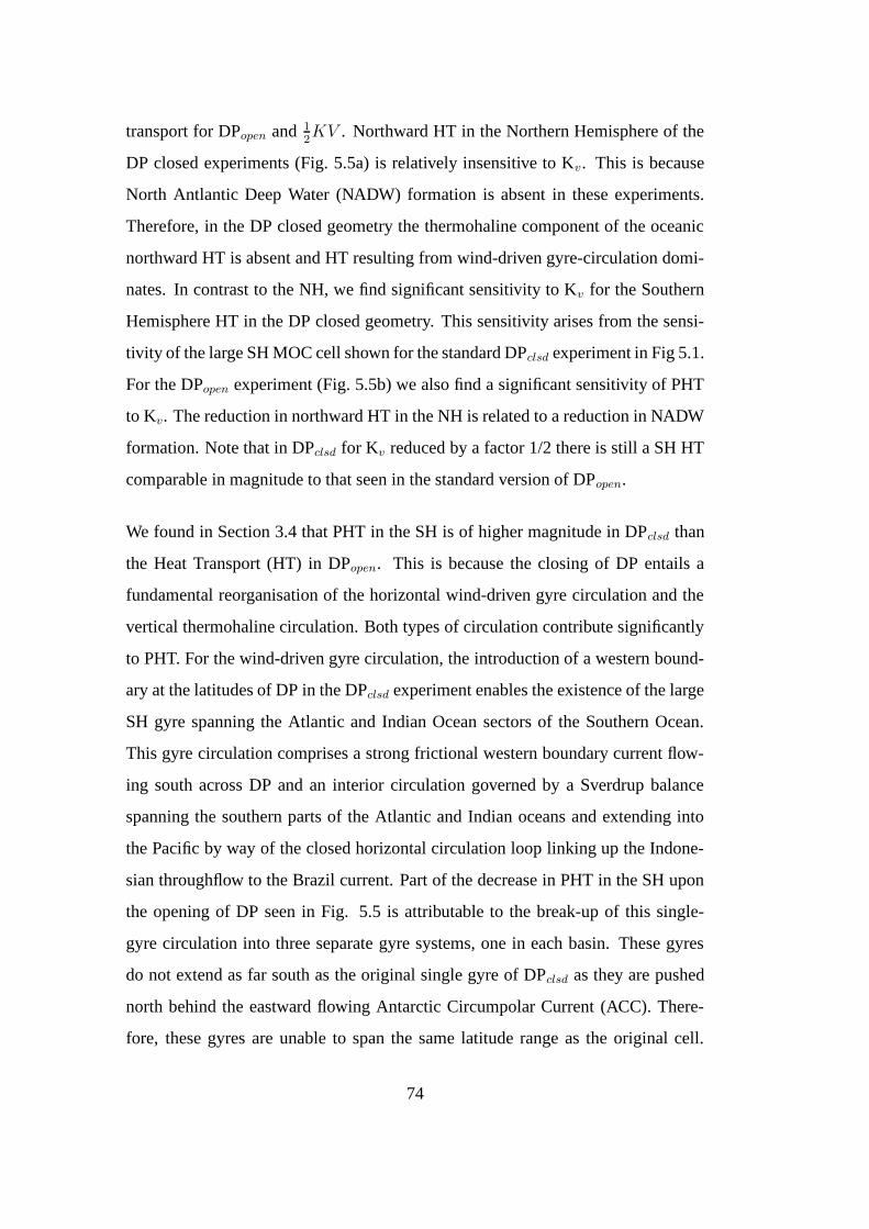
transport for DPopen and 1
2KV . Northward HT in the Northern Hemisphere of the
DP closed experiments (Fig. 5.5a) is relatively insensitive to Kv. This is because
North Antlantic Deep Water (NADW) formation is absent in these experiments.
Therefore, in the DP closed geometry the thermohaline component of the oceanic
northward HT is absent and HT resulting from wind-driven gyre-circulation domi-
nates. In contrast to the NH, we find significant sensitivity to Kv for the Southern
Hemisphere HT in the DP closed geometry. This sensitivity arises from the sensi-
tivity of the large SH MOC cell shown for the standard DPclsd experiment in Fig 5.1.
For the DPopen experiment (Fig. 5.5b) we also find a significant sensitivity of PHT
to Kv. The reduction in northward HT in the NH is related to a reduction in NADW
formation. Note that in DPclsd for Kv reduced by a factor 1/2 there is still a SH HT
comparable in magnitude to that seen in the standard version of DPopen.
We found in Section 3.4 that PHT in the SH is of higher magnitude in DPclsd than
the Heat Transport (HT) in DPopen. This is because the closing of DP entails a
fundamental reorganisation of the horizontal wind-driven gyre circulation and the
vertical thermohaline circulation. Both types of circulation contribute significantly
to PHT. For the wind-driven gyre circulation, the introduction of a western bound-
ary at the latitudes of DP in the DPclsd experiment enables the existence of the large
SH gyre spanning the Atlantic and Indian Ocean sectors of the Southern Ocean.
This gyre circulation comprises a strong frictional western boundary current flow-
ing south across DP and an interior circulation governed by a Sverdrup balance
spanning the southern parts of the Atlantic and Indian oceans and extending into
the Pacific by way of the closed horizontal circulation loop linking up the Indone-
sian throughflow to the Brazil current. Part of the decrease in PHT in the SH upon
the opening of DP seen in Fig. 5.5 is attributable to the break-up of this single-
gyre circulation into three separate gyre systems, one in each basin. These gyres
do not extend as far south as the original single gyre of DPclsd as they are pushed
north behind the eastward flowing Antarctic Circumpolar Current (ACC). There-
fore, these gyres are unable to span the same latitude range as the original cell.
74

This results in less southward HT in these gyres as this HT depends in part on the
thermal gradient across which the gyres operate. Furthermore, the delivery of heat
by the gyres no longer extends as far South as was possible in the DPclsd setting as
geostrophic flow is negligible across the DP gap. Furthermore, water resides for a
shorter period in the equatorial regions as more time is spent in north-south transit
as this latter trajectory has been tripled by splitting the cell in three. In contrast, the
original SH gyre circulation in DPclsd involves a larger and stronger gyre, where
water spends more time at lower latitudes, traversing long zonal trajectories there,
where warming occurs, thus enabling stronger warming in its western boundary
current region. Also, this gyre reaches further south across the latitudes of DP. The
resulting greater thermal contrast between the northern and southern gyre branches
must result in greater southward HT. Also, we found that DPclsd is characterised
by a large SH overturning cell. This circulation must also result in greater south-
ward HT in the ocean. We have found in Fig. 5.4 that the strength of the global
MOC circulation is sensitive to vertical mixing in DPclsd. Therefore, to examine
the resulting sensitivity of oceanic PHT to Kv, we have calculated northward heat
transport in a DP closed configuration for a set of values of Kv.
It is a well known fact that when HD is used in ocean models, unrealistically large
diapycnal fluxes of heat and salt occurs in regions with sloping isopycnal surfaces.
In particular, spurious heat transport across the ACC occurs, and is responsible for
an unrealistic component of the southward HT at these latitudes. This effect scales
with the depth of the isotherms north of DP as horizontal diapycnal mixing occurs
over a larger vertical surface area. In our implementation of GM, diffusion occurs
along isopycnals, and there is no background horizontal diffusion. Therefore, GM
eliminates the unrealistic horizontal diffusion across the steeply sloping isopycnals
in the Southern Ocean that occurs in HD. To examine the effect of choice between
HD and GM on HT, we show the northward oceanic heat transport in Figure 5.6
for (a) DPclsd HD and DPclsd GM, (b) DPopen HD, DPopen-DPclsd HD, DPopen GM
and DPopen-DPclsd HD, and (c) difference between the HD and the GM version
75

of DPopen and DPclsd . None of the curves show significant responses in the NH.
Therefore, we focus on the SH in the following. In agreement with the mentioned
absence of spurious diapycnal mixing by horizontal diffusion, there is a significant
reduction in southward HT in DPclsd upon the introduction of GM for DPclsd (a) and
DPopen (b). The difference plots shown in Fig. 5.6 (c) show that between around
55◦S and 65◦S, DPopen exhibits a stronger reduction in southward HT than DPclsd
in response to the removal of spurious horizontal diffusion of heat upon the intro-
duction of GM. This is because the spurious diapycnal mixing of heat across the
ACC is stronger in DPopen than in DPclsd due to the deeper isotherms in DPopen
(Fig. 3.1). From the difference plot for DPopen-DPclsd HD and DPopen-DPclsd GM
shown in Fig. 5.6 (b) we see that GM exhibits a stronger reduction in southward HT
between 55◦S and 65◦S than HD in response to the opening of DP. This is because
in HD, there are two opposing responses to the opening of DP:
1. An increase in southward HT occurs in response to the opening of DP due to
the interaction of horizontal diffusion with deepening isotherms north of DP
when DP is open in HD.
2. A reduction in southward HT occurs in response to the opening of DP due
to the absence of a strong SH MOC cell drawing surface waters across the
latitudes of DP.
Response (1) is absent in GM as there is no spurious diapycnal diffusion of heat
across sloping isopycnals. Response (2) is therefore not opposed by response (1) in
GM, resulting in a stronger reduction in in southward HT between 55◦S and 65◦S
than in HD. Also, we can expect stronger associated SH cooling effects to occur in
GM.
Figure 5.7 shows the MOC (yearly average) for (a,b) DPclsd GM and (c, d) DPclsd
GM with Kv reduced inside the Atlantic. The left column shows the global MOC
76

and the right column shows the Atlantic MOC. Kv is reduced via multiplication by
1/10. The DPclsd GM experiment yields a MOC circulation that is qualitatively sim-
ilar to that found in DPclsd. A large interhemispheric SH overturning cell dominates
global MOC circulation (Fig. 5.7a) and penetrates to high northern latitudes in the
Atlantic (Fig. 5.7b). The strength of this cell, 38 Sv, is significantly smaller than in
DPclsd. We have attempted to excite a transition to a NH overturning state using a
temporary fresh water perturbation in DPclsd GM without success. Around 11 Sv
of AABW upwells inside the Atlantic. Taking a value of 26 Sv, AABW formation
is significantly reduced when Kv is reduced by 1/10 inside the Atlantic (Fig. 5.7c).
In addition, NH overturning circulation appears. In the Atlantic (Fig. 5.7d), 7 Sv
of deepwater formation occurs and 4 Sv of deepwater outflow occurs. A negligible
amount of AABW enters the Atlantic. This shows that when using GM, AABW
can be removed from the Atlantic by reducing Kv there. The reduced ability of
AABW to upwell across 2000 m inside the Atlantic impairs its competitive advan-
tage for circulation inside that basin. This enables the development of a NADW
cell. We have run an identical experiment using a reduction of 1/10 for Kv inside
the Atlantic for HD, and could not reproduce the result found for GM. In Chapter 6
we will see that GM enables a NADW formation process in this model that is less
sensitive to the development of a fresh water lense at the surface than in HD. This
could explain the greater propensity of NADW to form in our DPclsd GM experi-
ment when Kv is sufficiently reduced inside the Atlantic. The strength of the SH
overturning cell in DPclsd GM (38 sv) is significantly lower than in DPclsd HD (58
Sv). A similar reduction in NH overturning is observed in DPopen when using GM
and can be attributed to a reduction in potential energy available to the overturning
due to a shallowing of the thermocline (see Fig 5.8). Another factor affecting MOC
strength is the substantial decrease in diapycnal mixing arising from the adoption
of the GM parametrisation.
Figure 5.8 shows the zonal mean of the sea temperature (degrees C) for (a) DPclsd
HD and (b) DPclsd GM. A significant shallowing of the isotherms occurs when GM
77

is used. This is because the quasi-advective velocities used to model the effect of
baroclinic instability in GM have a tendency to flatten isopycnals. As the surface
density of the ocean is largely driven by local air-sea fluxes of heat and salt, isopy-
cnals outcrop at similar latitudes as when the GM velocities are absent. Therefore,
isopycnals shoal in response to the flattening tendency of the GM velocities. Note
that the surface fluxes do not undergo a strong poleward shift upon the introduction
of the GM velocities.
b. Sensitivity of the DPopen-DPclsd results to mixing parametrisation
We saw in Chapter 3 that the opening of DP at the Eocene/ Oligocene boundary may
have had a significant impact on global climate. Here, we examine the sensitivity
of this result with respect to the subgrid-scale mixing parametrisations we use. In
particular, we examine the effect of a reduction in Kv by 1/2 and the introduction of
GM on Sea Surface Temperature (SST), Surface Air Temperature (SAT) and sea-
ice frequency. Reducing Kv by a factor 1/2 for a DP open and closed geometry
allows us to examine the climatic response to the opening of DP in this scenario
of reduced vertical mixing. We denote the reduced KV version of DPclsd by DPclsd
1
2KV and the reduced KV version of DPopen by 1
2KV . We find that reducing Kv
results in reduced oceanic heat transport to high latitudes. This, in turn, leads to a
significantly weaker SAT response to the opening of DP. Introducing GM, on the
other hand, results in a stronger SAT response. This stands in contrast to the weaker
SH cell in DPclsd GM (section a).
Figure 5.9 shows the meridional overturning streamfunction (yearly average) for
(Fig. 5.9a) 1
2KV shown for the global domain, (Fig. 5.9b) 1
2KV shown for the At-
lantic, (Fig. 5.9c) DPclsd1
2KV shown for the global domain (Fig. 5.9d) DPclsd
1
2KV
shown for the Atlantic. Global meridional overturning for 1
2KV (Fig. 5.9a) is simi-
lar for DPopen, but exhibits reduced NH sinking. Atlantic MOC (Fig. 5.9b) also has
78

all the characteristics of the Atlantic overturning in the standard DPopen experiment,
but with a reduced NADW formation of 11 Sv and 4 Sv NADW outflow. AABW
inflow is reduced to 3 Sv. SH sinking in DPclsd1
2KV (Fig. 5.9c) is reduced to 47
Sv, and AABW inflow into the Atlantic (Fig. 5.9d) is less affected by the reduction
in vertical mixing and takes a value of 10 Sv. The reduction in NADW formation
in DPopen is a result of the reduced upwelling at lower latitudes in the world ocean
due to the lower values of Kv used globally. Similarly, the reduced SH overturn-
ing in DPclsd arises from reduced low latitude upwelling of deep water across the
thermocline.
Figure 5.10 shows the ocean barotropic streamfunction for (a) DPclsd1
2KV , (b) the
difference DPclsd1
2KV minus DPclsd, (c) DPclsd GM and (d) the difference DPclsd
GM minus DPclsd. The circulation for DPclsd1
2KV is similar to DPclsd, with a large
gyre spanning the southern parts of the Indian and Atlantic oceans, a strong Brazil
current of 50 Sv and a gyre of 30 Sv near the Ross Sea. Interestingly, this gyre is
significantly reduced in strength when compared to DPclsd (Fig. 5.10b), where a 60
Sv gyre occurs near the Ross sea. The strength of this gyre is linked to the thermo-
haline MOC circulation (Saenko, personal communication) via the joint effect of
baroclinicity and relief (JEBAR), and the reduction in AABW formation observed
in Fig. 5.9 could be the cause of the reduction in strength of this gyre. There is
also a 10 Sv reduction in the Brazil current, seen from the 10 Sv gyre spanning the
southern Atlantic and Indian oceans in the difference plot. Furthermore, the EAC is
reduced by 5 Sv. For GM (c) we also see a reduction to 30 Sv in the strength of the
Gyre near the Ross Sea. Horizontal mass transport in DPclsd is surprisingly similar
when Kv is halved. This means that we can expect climatic changes in response to
the opening of DP that arise from an adjustment of the gyre circulation to be similar
for DPclsd and DPclsd1
2KV .
Figure 5.11 shows the annual average of sea surface temperature difference (at 25-
m depth;◦C) for (a) DPopen minus DPclsd (HD), (b) 1
2KV minus DPclsd
1
2KV and
79

(c) DPopen minus DPclsd GM. The standard DPopen minus DPclsd case (a) is sim-
ilar to Version 2.5 with a large area of cooling in the Atlantic and Indian sectors
of the Southern Ocean, taking a maximum value of 9.5◦C. A large area of warm-
ing occurs south of Australia, taking a maximum value of 3.9◦C. As in Version
2.5 of the model, the 6.7◦C warming in the North Atlantic is related to the in-
crease in oceanic heat transport resulting from the onset of NADW formation upon
opening DP in DPopen. Interestingly, this warming is significantly reduced for the
1
2KV experiments (Fig. 5.11b), where only 3.5◦C warming occurs in the Atlantic.
This is because the reduction we apply to Kv results in a significant reduction in
NADW formation and therefore PHT in 1
2KV (see Fig. 5.5). A cooling in 1
2KV -
DPclsd1
2KV similar to DPopen-DPclsd (Fig. 5.11a) of 8.7◦C occurs in the Atlantic
and Indian sectors of the Southern Ocean. The cooling at high latitudes west of
the DP observed in DPopen-DPclsd (Fig. 5.11a), however, is significantly reduced
in magnitude and extent. This is because this cooling, unlike the cooling at mid-
southern latitudes east of South America, is strongly determined by the strength of
the AABW cell, which is reduced in this experiment. This reduction in cooling
is consistent with the reduction of southward HT in response to a reduction in Kv
seen in Fig 5.5. The robustness of the SH cooling at lower latitudes with respect to
vertical mixing indicates that this cooling is strongly related to changes in the wind-
driven gyre circulation caused by the opening of the DP and does not have a strong
thermohaline component. The warming south of Australia in 1
2KV -DPclsd
1
2KV is
similar in magnitude (3.6◦C) to DPopen-DPclsd, and greater in extent. The warming
in the North Atlantic (6.4◦C) for the GM experiment (Fig. 5.11c) is similar to the
standard HD version (Fig. 5.11a). The GM experiment also shows an area of cool-
ing of 9.7◦C in the Atlantic and Indian sectors of the Southern Ocean, somewhat
larger than, and similar in extent to the previous experiments. The cooling west
of DP, however, is significantly larger than that observed in the HD experiments
(Fig. 5.11a). This larger cooling is a result of the stronger reduction in southward
PH across the latitudes of DP seen in Fig 5.6. The 3.6◦C warming south of Aus-
tralia is similar in magnitude, but significantly smaller in extent when compared to
80

the HD experiments. This is because the ACC is not steered too far south in the
GM version of the experiment (see Chapter 3).
Figure 5.12 shows the annual-mean of the sea-ice frequency difference DPopen-
DPclsd for (a) HD, (b) 1
2KV and (c) GM. Similar to model Version 2.5 we find a
significant reduction of sea-ice frequency in the North Atlantic in response to the
opening of DP in the standard DPclsd minus DPopen comparison (Fig. 5.12a). This
results from an increase in northward HT due to the existence of NADW formation
in DPopen, a feature absent in DPclsd. In the SH an increase in sea-ice frequency oc-
curs in response to a reduction in southward HT in combination with a smaller area
of sea-ice decrease corresponding to the area of warming south of Australia. The re-
duction in sea-ice frequency in the North Atlantic is significantly less pronounced in
the 1
2KV minus DPclsd
1
2KV difference plot (Fig. 5.12b). This is due to the weaker
NADW formation in 1
2KV . By the same mechanism, in the SH a smaller increase
in sea-ice extent occurs in response to the opening of DP (Fig. 5.12b), especially
west of DP. This is due to a reduction in southward HT in DPclsd1
2KV compared
to DPclsd. In addition, the area of sea-ice frequency increase in response to opening
the DP is larger. For GM (Fig. 5.12c) we find similar results to HD, but with a more
pronounced sea-ice increase west of DP. This is due to the stronger SST cooling in
GM. Furthermore, GM shows a less extensive sea-ice frequency decrease south of
Australia. This results from less pronounced warming there upon the opening of
the DP.
Figure 5.13 shows the annual mean surface air temperature difference (◦C) for
DPopen-DPclsd for (a) HD, (b) 1
2KV and (c) GM. The standard DPopen-DPclsd ex-
periment yields similar results to Version 2.5 with a NH warming of 6◦C and high
latitude SH cooling of 8◦C. The area of warming south-southwest of Australia at-
tains a value of 4◦C. For the 1
2KV minus DPclsd
1
2KV comparison we find a sig-
nificantly reduced warming in the North Atlantic in response to the opening of the
DP, attaining only a maximum value of 1◦C. This is due to the less pronounced
81

SST warming of 3.5◦C there (Fig 5.11) and a significantly smaller sea-ice response
in this area. As described in Section 3.4, the effect on SAT of the SST response to
opening DP can be amplified by changes in sea-ice frequency due to a positive feed-
back where decreased sea-ice extent leads to warmer temperatures and thus further
sea-ice melt-back (via sea-ice albedo anomalies). Conversely, the insulating effect
of sea-ice leads to colder temperatures by removing the mitigating influence of the
ocean during cold winter months, thus amplifying the SST cooling. This feedback
mechanism explains the significantly smaller SAT response in the North Atlantic
of 1◦C to the opening of DP when Kv is reduced by a factor of 1/2. Similarly, the
smaller cooling response at the high southern latitudes west of DP of 5◦C derives
from smaller SST cooling in combination with a smaller sea-ice response. This area
of cooling is also of much smaller spatial extent. Therefore the 1
2KV -DPclsd
1
2KV
comparison lends less support to Kennett (1977)’s hypothesis that the opening of
DP contributed to the glaciation of Antarctica. The SAT cooling at lower southern
latitudes of 6◦C is more similar to the standard DPopen-DPclsd HD response (7◦C).
Here, the thermohaline circulation and sea-ice exert a weaker influence. The area
of SAT warming south of Australia, however, is of greater spatial extent than in the
standard DPopen-DPclsd comparison. For the GM experiment (Fig. 5.13 c) we find
a similar NH SAT warming of 6◦C, but a deeper maximum SH cooling of 12◦C.
This is related to the deeper SST cooling and the stronger sea-ice response for the
GM experiment (fig 5.12). Lower southern latitude cooling, however, is similar
to the standard DPopen-DPclsd comparison. Also, the warming south of Australia
takes a maximum value of only 2◦C and is of significantly smaller spatial extent
than the standard DPopen-DPclsd experiment. The GM experiment thus lends more
support to Kennett (1977)’s hypothesis. To summarise the net effect of these SAT
changes, we plot in Figure 5.14 the zonal mean of the annual mean SAT difference
(◦C) for DPopen-DPclsd, 1
2KV - DPclsd
1
2KV and DPopen GM -DPclsd GM. The weak
SH cooling of 1.1◦C in response to opening DP in the 1
2KV experiments compared
to 3.6◦C for the standard HD experiments indicates that this experiment has weaker
support for Kennett’s hypothesis. Also, we conclude from this that the quantitative
82

results for experiment DPopen-DPclsd described in Chapter 3 are sensitive to Kv, al-
though the conceptual result remains robust. The GM experiment, however, attains
a maximum zonal mean SH cooling of 4.4◦C, a value larger than the 3.6◦C found
for the HD experiment. Therefore, the GM experiment lends somewhat more sup-
port to Kennett’s hypothesis than the HD standard experiment. We have seen from
the horizontal plot shown in Fig 5.13 that this is due to an increased SAT cooling
at high southern latitudes west of DP, in combination with a strong reduction in
magnitude and spatial extent of the SAT warming south of Australia.
5.5. Discussion and Conclusions
The strength of the large SH MOC cell of DPclsd is sensitive to Kv and provides
a reasonable fit to Bryan’s 2/3-power law for a range of values. The cell remains
strong, however, even under a reduction of Kv by a factor 1/3. Furthermore, the cell
maintains its characteristic interhemispheric domain of global MOC circulation.
A per-basin reduction of Kv shows that the effect of reducing Kv is additive in a
DPclsd- geometry and that when Kv is reduced globally, a large proportion of the
resulting reduction in SH overturning is attributable to changes in the Indian and
Pacific oceans alone. The sensitivity of SH overturning to Kv also translates into
a sensitivity of southward HT to Kv. This is because this HT depends not only on
the gyre circulation, but also on the strength of the MOC. Smaller values of Kv in
DPclsd result in a weaker SH overturning and therefore a reduction in PHT. The
1
2KV experiments exhibit a significantly weaker response to the opening of DP in
both hemispheres for several key variables. SAT response is particularly weak due
to feedbacks operating in the model climate. NADW formation, however, is too
weak in 1
2KV in the control DPopen experiment (11 Sv). It is interesting to note
that the large area of SH SST cooling in the southern Indian and Atlantic oceans is
relatively robust with respect to Kv. This indicates that this cooling results largely
83

from a reorganisation of the horizontal subtropical gyre circulation in response to
the opening of the DP. This reorganisation is very similar for Kv=1/2 and Kv=1
(Fig. 5.9), and is therefore a feature that is relatively insensitive to the choice of
vertical mixing rate.
Despite the weaker overturn in DPclsd GM, this experiment exhibits a relatively
strong SST cooling at high southern latitudes west of DP in response to the opening
of DP. We have seen in Fig. 5.6 that GM exhibits a stronger reduction in Southern
Hemisphere HT in response to the opening of DP due to the absence of spurious
diapycnal mixing of heat across the ACC. Therefore, despite the reduced strength
of the SH overturning cell in DPclsd GM compared to DPclsd HD, GM manages
to maintain a somewhat stronger SST cooling at the high latitudes west of DP in
response to the opening of DP under GM. Due to the absence of spurious mixing of
heat across the ACC, we regard this result as more realistic.
It should be noted that the sensitivity study of this Chapter is not exhaustive. Among
other factors we have not considered here, changes in zonal resolution and associ-
ated horizontal viscosity could also affect meridional HT in western boundary cur-
rents. Kamenkovich (2000) find a noticeable increase in the Atlantic basin’s heat
transport upon an increase in zonal resolution and decrease in horizontal viscosity.
A study of the sensitivity of our results to this change remains to be done. In partic-
ular, an increase in zonal resolution coupled to a reduction in horizontal viscosity
in a GM configuration of the model may yield significantly stronger cooling upon
the opening of DP when compared to standard coarse resolution HD experiments.
Furthermore, our results would benefit from an increase in the understanding of the
effect of the thermal conductivity of snow on Antarctic sea-ice (Wu et al. 1999) as
changes in model parametrisations of the thermal conductivity of snow could affect
the sea-ice response to the opening of DP shown in Chapter 3 and therefore also the
amplified SAT response in winter.
In conclusion, we have found that the results of Chapter 3 and Chapter 4 are sensi-
84

tive to Kvand the choice of the lateral diffusion scheme. The mid-latitude cooling
associated with the readjustment of the subtropical gyres is significantly less sensi-
tive to vertical mixing than the high southern latitude cooling west of the DP. Larger
values of Kv lead to a strengthening of the large SH cell found in DPclsd and associ-
ated increases in PHT. Smaller values of Kv (such as half the standard value) yield
a significantly less pronounced response to the opening of the DP. The choice of
subgrid-scale mixing parametrisation, in particular HD vs. GM, does not alter our
results in a fundamental way, but GM lends somewhat more support to Kennett’s
hypothesis by exhibiting a stronger SH cooling.
85

60S 30S EQ 30N 60N
4
3
2
1
LATITUDE
DE
PT
H (
km)
0
0
0
0 0
00
00
0−58
−54
−50
−46
−42 −4
2
−38−30 −34−26−2
2−1
8
−14−10 −6
−2
2
(a) global
30S EQ 30N 60NLATITUDE
0
0
0
00
−13
−10
−9
−8−7 −6−5
−4
−3−2−1
1
(b) Atlantic
Figure 5.1: Meridional overturning streamfunction DPclsd in model version 2.6
(yearly average) for (a) a global domain and (b) the Atlantic. Values are given
in Sv (1 Sv = 106 m3 sec−1).
60E 120E 180 120W 60W 90S
60S
30S
EQ
30N
60N
90N
LONGITUDE
LAT
ITU
DE
−80−70−60
−50 −50−50−40
−40−40−30
−30−30
−30−20 −20
−20 −20
−10 −10
−10−1
0
0
0
0
0
0
0
0 0
0
0
0
00
10 1010 10
1010
20
20
20
20
20 20 30
30
405060
Figure 5.2: Year average of the ocean barotropic streamfunction for DPclsd. Values
are given in Sv (1 Sv = 106 m3 sec−1).
86

4
3
2
1
DE
PT
H (
km)
0 0 0
0 0
0
0
0
0
0
00
0
00−54 −
46−
42 −42
−38
−34−30−26−22−18−14−10−6
−2
2
(a) Kv reduced in Atlantic
00
0
0 0 0
0
0 0 0
0
0
−9
−7−6
−5 −4
−3
−2
−1
1
(b) Kv reduced in Atlantic
4
3
2
1
DE
PT
H (
km)
0 0 0
0
0
0
0
0
00
00
−46
−42
−38
−34 −3
4
−30−26−22−18−14−10−6−2
2
(c) Kv reduced in Pacific
00
0
0 0 0
0000
−13 −
11
−10
−9 −8
−7−6−5 −4
−3−2
−6
−1
1
(d) Kv reduced in Pacific
60S 30S EQ 30N 60N
4
3
2
1
LATITUDE
DE
PT
H (
km)
00
0
0 0
0
0
0
00
0
−42−38
−30
−30−26
−22−18−14−10−6−2
(e) Kv reduced globally
30S EQ 30N 60NLATITUDE
0
0
0
0
0
000
−9
−7−
6−5
−4 −3
−2
−1
1
(f) Kv reduced globally
Figure 5.3: Meridional overturning streamfunction (yearly average) for (left col-
umn) a global domain and (right column) the Atlantic. Experiments are shown by
row: (a,b) DPclsd1
3KVAtl, (c, d) DPclsd
1
3KVIP and (e,f) DPclsd
1
3KVglob. Kv is
reduced via multiplication by 1/3. Values are given in Sv (1 Sv = 106 m3 sec−1).
87

0.25 0.5 0.75 1 1.25 1.5 1.75 2 2.25 2.5 2.75 3
40
50
60
70
80
90
100
110
120
Sv
factor
Figure 5.4: SH overturning in DPclsd against (global) multiplicative factor for Kv.
Both axes use a logarithmic scale. Values are given in Sv (1 Sv = 106 m3 sec−1).
−90 −60 −30 0 30 60 90−3
−2.5
−2
−1.5
−1
−0.5
0
0.5
1
1.5
Latitude
PW
(a) DPclsd
−90 −60 −30 0 30 60 90Latitude
(b) DPopen
1.2510.50.3
10.5
Figure 5.5: Northward oceanic heat transport in HD experiments for (a) DPclsd Kv
multiplied globally by a factor 1.25, 1, 0.5 and 0.3 and (b) DPopen resp. 1
2KV , where
Kv is multiplied globally by a factor 1 resp. 0.5. The legend lists the multiplication
factors used with respect to the standard values of Kv.
88

−3
−2
−1
0
1
PW
(a) DPclsd
−3
−2
−1
0
1
PW
(b) DPopen
and DPopen
−DPclsd
−90 −60 −30 0 30 60 90−1.5
−1
−0.5
0
0.5
Latitude
PW
(c) HD−GM
DPclsd
HDDP
clsd GM
DPopen
HDDP
open−DP
clsd HD
DPopen
GMDP
open−DP
clsd GM
HD−GM DPopen
HD−GM DPclsd
Figure 5.6: Northward oceanic heat transport in HD experiments for (a) DPclsd
HD (solid) and DPclsd GM (dashed), (b) DPopen HD (solid, black), DPopen-DPclsd
HD (solid, blue), DPopen GM (dashed) and DPopen-DPclsd HD (dashed, blue), and
(c) difference between the HD and the GM version of DPopen (solid) and DPclsd
(dashed).
89

4
3
2
1
DE
PT
H (
km)
0
0
0
0
0
0
0
0
00
0
−38
−34 −30
−30 −
34−3
8
−26−22−18−14−10−6−2
2
−10
(a) DPclsd
GM
0
0
0
0
−11
−10
−8 −7
−6−5
−4−3
−2−1
2
1
(b) DPclsd
GM
60S 30S EQ 30N 60N
4
3
2
1
LATITUDE
DE
PT
H (
km)
0
0
0 0 0 0
0
0
0
00
0
−26−22
−18
−18
−14−10−6
−2
−2
−30
−26−22
−18
−14
−10
−6
−2
2
6−10
14(c) DP
clsd GM Kv reduced Atl
30S EQ 30N 60NLATITUDE
0
0
0 0 0
0
0 0
0
576
4 321
−1−1
(d) DPclsd
GM Kv reduced Atl
Figure 5.7: Meridional overturning (yearly average) for (a,b) DPclsd GM and (c,
d) DPclsd GM Kv reduced inside the Atlantic. The left column shows the global
domain and the right column shows the Atlantic domain. Kv is reduced via multi-
plication by 1/10. Values are given in Sv (1 Sv = 106 m3 sec−1).
90

°C
0
5
10
15
20
25
°C
0
5
10
15
20
25
60S 30S EQ 30N 60N
4.5
4
3.5
3
2.5
2
1.5
1
0.5
LATITUDE
DE
PT
H (
km)
0
0
02
2
4
4
6
6
8
810 1214161820222426(a) DP
clsd HD
60S 30S EQ 30N 60NLATITUDE
0
02
24
4
6
6
8
8
101214161820222426(b) DP
clsd GM
Figure 5.8: Zonal mean of sea temperature (◦C) for (a) DPclsd HD and (b) DPclsd
GM.
91

4
3
2
1
DE
PT
H (
km)
0
0 0
0
0
0
0
0
0
0
0
00
8
52
−1−4−7
−7
−4
−1
−10−13
29
23
2017
14
1185 2
−1
−4
−10
−4
−4
−7−1
(a) DPopen
Kv reduced globally
00
0
0
0
0 0
0
0 0
0
11
98
7654321
54321
−1−2−3−2−1
−3 −3
(b) DPopen
Kv reduced globally
60S 30S EQ 30N 60N
4
3
2
1
LATITUDE
DE
PT
H (
km)
0
0
0
0 0
00
0
2−1−4−7
−10
−13−16
−19
−22
−25−28
−34
−31
−46 −
34
−31
−25−19
−1617
−4−1
(c) DPclsd
Kv reduced globally
30S EQ 30N 60NLATITUDE
0
0 0
0
0 0
0
0
0 1
−1−2−3
−4
−5−6
−7
−10
(d) DPclsd
Kv reduced globally
Figure 5.9: Meridional overturning streamfunction (yearly average) for (a) 1
2KV
shown for the global domain, (b) 1
2KV shown for the Atlantic, (c) DPclsd
1
2KV
shown for the global domain (d) DPclsd1
2KV shown for the Atlantic. Values are
given in Sv (1 Sv = 106 m3 sec−1).
92

90S
60S
30S
EQ
30N
60N
90NLA
TIT
UD
E
−80−70−60−50 −50
−50
−40 −40
−40
−30
−30 −30
−30−20 −20
−20 −20−1
0
−10
−10 −10
00
0
00
0
0
0
00
0
00
101010 10
1010
20
20
20
20
20 20 30
30
405060
(a) Control
90S
60S
30S
EQ
30N
60N
90N
LAT
ITU
DE
−70−60−50 −50−40 −40
−40
−30−30
−30−30−20 −20
−20−20−10 −10
−10 −10
0 0
0
0
00
000
0
0
0
00
0
0
1010 10
10
1010
10
20
20
30
30(b) 1/2KV
60E 120E 180 120W 60W 90S
60S
30S
EQ
30N
60N
90N
LONGITUDE
LAT
ITU
DE
−20 −15−10−5−5
00
00
0
0
0
0
0
0
0
0
0
0 00
0
0
0
0
00
00
0
0
0 0
00
0
5 55
5
5
10
(c) 1/2KV−control (difference)
Figure 5.10: Year average (Sv) of the ocean barotropic streamfunction for (a) DPclsd
1
2KV , (b) difference DPclsd
1
2KV -DPclsd, (c) DPclsd GM and (d) difference DPclsd
GM-HD. Values are given in Sv (1 Sv = 106 m3 sec−1).
93

°C
−5
0
5
°C
−5
0
5
°C
−5
0
5
90S
60S
30S
EQ
30N
60N
90N
LAT
ITU
DE
(a) HD
90S
60S
30S
EQ
30N
60N
90N
LAT
ITU
DE
(b) 1/2 KV
60E 120E 180 120W 60W 90S
60S
30S
EQ
30N
60N
90N
LONGITUDE
LAT
ITU
DE
(c) GM
Figure 5.11: Annual average of sea surface temperature difference (at 25-m depth;
◦C) for (a) DPopen-DPclsd HD, (b) 1
2KV -DPclsd
1
2KV and (c) DPopen-DPclsd GM.
94

−1
−0.5
0
0.5
1
−1
−0.5
0
0.5
1
−1
−0.5
0
0.5
1
90S
60S
30S
EQ
30N
60N
90N
LAT
ITU
DE
(a) HD
90S
60S
30S
EQ
30N
60N
90N
LAT
ITU
DE
(b) 1/2KV
60E 120E 180 120W 60W 90S
60S
30S
EQ
30N
60N
90N
LONGITUDE
LAT
ITU
DE
(c) GM
Figure 5.12: Annual-mean sea ice frequency difference DPopen- DPclsd for (a) HD,
(b) HD, Kv multiplied by factor 0.5 ( 1
2KV ) and (c) GM.
95

°C
−10
−5
0
5
10
°C−10
−5
0
5
10
°C
−10
−5
0
5
10
90S
60S
30S
EQ
30N
60N
90N
LAT
ITU
DE
−6−5−5
−4−4
−3
−3
−3
−2
−2
−1
−1
0
0
11
22
11
3
2
4
−6
5
3
3
−7
64
4 −8
(a) HD
90S
60S
30S
EQ
30N
60N
90N
LAT
ITU
DE
−6
−5
−4
−3
−3
−2
−2
−1
−1
0
0
0
11
1
1
22
3 −44
(b) HD, Kv reduced by factor 0.5
60E 120E 180 120W 60W 90S
60S
30S
EQ
30N
60N
90N
LONGITUDE
LAT
ITU
DE
−6−6 −5−5−4−4
−3−3−2
−2 −1−1 00
11
223
−7
1
4
−8−9
3
5
−10
12
−11−7
64
−12
(c) GM
Figure 5.13: Annual mean surface air temperature difference (◦C) for a) DPopen-
DPclsd, (b) 1
2KV - DPclsd
1
2KV and (c) DPopen-DPclsd GM.
96

−90 −60 −30 0 30 60 90−5
−4
−3
−2
−1
0
1
2
3
LATITUDE
°C
DPopen
−DPclsd
1/2KV−DPclsd
1/2KVDP
open−DP
clsd GM
Figure 5.14: Zonal mean of the annual mean surface air temperature difference (◦C)
for DPopen-DPclsd (blue), 1
2KV - DPclsd
1
2KV (black) and DPopen-DPclsd GM (red).
97

Chapter 6
Can isopycnal mixing control the
stability of the thermohaline
circulation in ocean climate models?
6.1. Abstract
Convective adjustment arising from static instability during winter is thought to
play a crucial role in the formation of NADW. In Ocean General Circulation Mod-
els (OGCMs), a strong reduction in convective penetration depth arises when hori-
zontal diffusion (HD) is replaced by Gent and McWilliams (GM) mixing to model
the effect of mesoscale eddies on tracer advection. In areas of sinking, the role of
vertical tracer transport due to convection is largely replaced by the vertical compo-
nent of isopycnal diffusion along sloping isopycnals. Here, we examine the effect
of this change in tracer transport physics on the stability of NADW formation under
fresh water (FW) perturbations of the North Atlantic (NA) in a coupled model. We
find a significantly increased stability of NADW to FW input when GM is used in
98

spite of GM experiments exhibiting consistently weaker NADW formation rates in
unperturbed steady states. We also find a significant increase in NADW stability
upon the intoduction of isopycnal diffusion seen in the absence of GM. This indi-
cates that isopycnal diffusion of tracer rather than isopycnal thickness diffusion is
responsible for the increased NADW stability observed in the GM run. This re-
sult is robust with respect to the choice of isopycnal diffusion. Also, the NADW
behaviour in the isopycnal run, which includes a fixed background horizontal diffu-
sivity, demonstrates that HD is not responsible alone for reducing NADW stability
when simple horizontal diffusion is used. Our results suggest that care should be
taken when interpreting the results of coarse grid models with regard to NADW
sensitivity to FW anomalies.
6.2. Introduction
The deep ocean is ventilated by high latitude sinking of cold and dense water. Con-
vective overturning of the water column during winter in the North Atlantic (NA)
and the abyssal outflow of cold shelf water formed in the Ross and Weddell Seas
and off Adelie Land around Antarctica contribute to much of this process. Up-
welling into the ocean’s thermocline and wind driven upwelling in the Southern
Ocean (SO) are responsible for the eventual removal of this cold and dense water.
During sinking, the release of potential energy by convective overturning leaves
vertically homogeneous tracer distributions through gravitationally unstable parts
of the water column. Coarse resolution OGCMs prohibit explicit representation
of this process. Instead, enhanced vertical diffusivity (e.g. Hirst and Cai 1994) or
a convective adjustment algorithm such as that suggested by Rahmstorf (1993) is
employed for unstably stratified vertically adjacent cells.
In a model, deep convection may facilitate significant inflow and sinking at the top
of the water column and outflow at the bottom. The outflow of dense water into
99

the lighter surrounding area and its subsequent propagation at the bottom of the
overturned column allows shallower inflow into the overturned areas by continuity
of mass. Also, this artificial convection acts to damp the impact of surface fluxes
in water mass formation regions by vertically mixing surface properties deep into
the interior. For example, North Atlantic Deep Water (NADW) formation occurs
in a region of net precipitation (Schmitt et al. 1989). With a positive feedback of
increasingly stable stratification, net precipitation can lead to reduced frequency,
reduced spatial extent and reduced depth of convection, leading to an eventual shut-
down of NADW sinking (e.g. Rahmstorf 1996; Zang et al. 1993).
Despite the importance of convection in models in transforming water-mass prop-
erties at high latitudes, the process alone does not set water-mass formation rates.
For example, Bryan (1987) showed that the strength of the meridional overturning
(MOC) decreases with decreasing vertical diffusivity. Similarly, model studies indi-
cate the role of Southern Ocean (SO) winds in setting at least part of the strength of
NADW formation (e.g. Toggweiler and Samuels 1995). Therefore, even though NA
convection may enable and enhance sinking, the process alone does not prescribe a
sinking rate. Indeed, ocean climate models are generally hydrostatic, with convec-
tive overturn occurring independently of any calculations of vertical velocity, which
is instead determined diagnostically by the continuity equation.
Ocean General Circulation Models (OGCMs) representing subgrid scale turbulent
mixing of tracer properties by way of a horizontal diffusivity generally overesti-
mate the extent and depth of convective overturning in the world ocean. Reduced
areas of convection occur with the introduction of the parametrisation of Gent and
McWilliams (1990, hereafter GM) where eddy-induced tracer advection terms, with
a tendency to flatten isopycnals, are introduced. The first study to show a sharp
reduction in mid and high-latitude convection with introduction of GM was Dan-
abasoglu et al. (1994). Subsequent studies (e.g. England 1995; Hirst and Cai 1994;
Danabasoglu et al. 1994; Duffy et al. 1995; England and Rahmstorf 1999; Sørensen
100
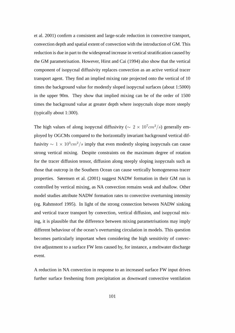
et al. 2001) confirm a consistent and large-scale reduction in convective transport,
convection depth and spatial extent of convection with the introduction of GM. This
reduction is due in part to the widespread increase in vertical stratification caused by
the GM parametrisation. However, Hirst and Cai (1994) also show that the vertical
component of isopycnal diffusivity replaces convection as an active vertical tracer
transport agent. They find an implied mixing rate projected onto the vertical of 10
times the background value for modestly sloped isopycnal surfaces (about 1:5000)
in the upper 90m. They show that implied mixing can be of the order of 1500
times the background value at greater depth where isopycnals slope more steeply
(typically about 1:300).
The high values of along isopycnal diffusivity (∼ 2 × 107cm2/s) generally em-
ployed by OGCMs compared to the horizontally invariant background vertical dif-
fusivity ∼ 1 × 103cm2/s imply that even modestly sloping isopycnals can cause
strong vertical mixing. Despite constraints on the maximum degree of rotation
for the tracer diffusion tensor, diffusion along steeply sloping isopycnals such as
those that outcrop in the Southern Ocean can cause vertically homogeneous tracer
properties. Sørensen et al. (2001) suggest NADW formation in their GM run is
controlled by vertical mixing, as NA convection remains weak and shallow. Other
model studies attribute NADW formation rates to convective overturning intensity
(eg. Rahmstorf 1995). In light of the strong connection between NADW sinking
and vertical tracer transport by convection, vertical diffusion, and isopycnal mix-
ing, it is plausible that the difference between mixing parametrisations may imply
different behaviour of the ocean’s overturning circulation in models. This question
becomes particularly important when considering the high sensitivity of convec-
tive adjustment to a surface FW lens caused by, for instance, a meltwater discharge
event.
A reduction in NA convection in response to an increased surface FW input drives
further surface freshening from precipitation as downward convective ventilation
101

is reduced. This positive feedback cycle is an efficient mechanism to shut down
convection and NADW sinking in models where NADW formation depends largely
on convection. Reduced convection inhibits NADW sinking, reducing the influx of
saline lower latitude water, causing further freshening of the surface region leading
to a further reduction in convection and sinking. This feedback is referred to as
“the positive salt feedback” (Rahmstorf and Willebrand 1995); it is also responsible
for the recovery of NADW formation that could occur after suppression. NADW
shutdown in response to FW perturbations is generally associated with a strong
permanent freshening of the NA (e.g. Manabe and Stouffer 1988; Sijp and England
2005). Indeed, these strong feedbacks allow small FW perturbations to cause large
surface salinity changes due to permanent circulation shifts. The apparent role of
convection in shutting down NADW formation in horizontal diffusion (HD) mod-
els stresses the importance of proper representation of this process in OGCMs, in
particular when considering its fundamentally different operation with the introduc-
tion of GM. Thus far, no study has assessed the sensitivity of NADW shutdown to
choice of mixing scheme in ocean GCMs.
Models employing GM generally exhibit less NADW formation and outflow than
models employing HD (e.g. Duffy et al. 1997). England and Rahmstorf (1999)
attribute this to flatter isopycnal surfaces under GM resulting in weaker interior
geostrophic flow. The reduction of diapycnal mixing in GM due to the absence of
horizontal diffusion across steeply sloping isopycnals in the Southern Ocean could
also be responsible for the reduction in NADW sinking rates (Duffy et al. 1997).
Indeed, Gerdes (1993) noted the importance of diapycnal mixing rather than ver-
tical mixing in setting this rate. Furthermore, the shoaling of Atlantic isopycnals
due to the removal of potential energy by eddy-induced advection may also re-
duce NADW formation (Gnanadesikan 1999). This is also illustrated in the study
of Kamenkovich and Sarachik (2004), wherein a reduction in NADW formation is
noted under GM as a result of denser AAIW associated with shoaling isopycnals
due to the tendency of GM velocities to flatten density surfaces. It remains un-
102

clear, however, whether the reduction of NADW formation and outflow under GM
is accompanied by a greater vulnerability of NADW to collapse in response to FW
perturbations. Such a FW anomaly might be due to a natural event such as melt-
water discharge or low-frequency precipitation variability, or it may be induced by
anthropogenic forcing (e.g. sea-ice and glacial meltwater).
The sensitivity to surface freshening associated with convection in HD may also be
different when isopycnal mixing (after Redi 1982) is employed. For instance, unlike
convection, isopycnal diffusion along sloping isopycnals can efficiently transport
surface properties deep into the interior in the absence of gravitationally unstable
stratification. Figure 6.1 shows a schematic representation of the processes respon-
sible for surface tracer removal in the NA when a tracer flux Fsurface (such as a FW
perturbation) is applied at the surface. A tracer flux Fhor due to horizontal advection
(incorporating GM advection) and horizontal mixing terms can remove the fresh-
water anomaly laterally. Fluxes due to vertical mixing (FKV ), isopycnal mixing
(FISO, in the case of GM or Redi (1982) mixing), convection (Fconv) and verti-
cal advection (Fw, including GM advection) can also contribute to tracer removal
from the NA surface region. The goal of this paper is to examine the sensitivity
of NADW collapse to the choice of model mixing scheme, and to further elucidate
the physical processes (Figure 6.1) responsible for controlling NADW shutdown in
ocean models.
The remainder of this paper is divided as follows. Section 6.3 covers a descrip-
tion of the model and experimental design. We will consider three main sets of
experiments, one employing horizontal diffusion, the second set employing along-
isopycnal diffusion and the third set adopting the parametrisation of GM. In sub-
section 6.4a we discuss the steady state fields under the three different subgid-scale
eddy parametrisations, focussing on surface tracer removal processes from the NA
catchment area. In subsection 6.4b we examine the hysteresis behaviour of the
three experiments under slowly varying FW perturbations applied to the NA. This
103

includes an assessment of the existence of multiple steady states under the applica-
tion of constant FW fluxes over prolonged periods of time. In subsection 6.4c we
apply FW pulses on a short timescale to the three experiments to examine FW flux
thresholds required for NADW collapse. Finally, section 6.5 consists of a discus-
sion and conclusions.
6.3. Model and Experimental Design
The simulations have been carried out using the Earth System Climate Model of
intermediate complexity of Weaver et al. (2001) described in Chapter 2. Here,
we use version 2.6. In order to examine the effect of different parametrisations
of tracer transport by mesoscale eddies on meridional overturning (MOC) stabil-
ity we integrated three versions of the model for 3000 years from idealised initial
conditions. During this integration, stability is tracked by monitoring key MOC
quantities such as the NADW formation and outflow rate. The first version, the
horizontal diffusion run (HD), employs the classical turbulent mixing parametrisa-
tion via constant diffusion along Cartesian coordinates. The diffusion coefficient in
both horizontal directions is Ah = 2 × 107cm2/s. We also analysed experiments
wherein this diffusion rate is halved to 1 × 107cm2/s. The second model version,
the GM case, employs the eddy-induced advection parametrisation of Gent and
McWilliams (Gent and McWilliams 1990), with isopycnal diffusion via a constant
coefficient of 2× 107cm2/s and isopycnal thickness diffusion with a constant coef-
ficient of 1×107cm2/s. Additional sets of GM experiments were also investigated
wherein along-isopycnal diffusion is reduced to 1×107cm2/s and 0.5×107cm2/s.
To isolate the effects of isopycnal diffusion, we have run a third set of experiments,
ISO, wherein isopycnal diffusion occurs with the same coefficient as used in GM,
but with the GM advection terms set to zero. In this third version we have to rein-
troduce horizontal diffusivity for numerical stability purposes. We employ the same
104

horizontal diffusivity used in HD, so that ISO is identical to HD, with the exception
of the additional effect of along-isopycnal diffusion. This pure isopycnal parametri-
sation for mixing was first suggested by Redi (1982) and later implemented in an
OGCM by Cox (1987). The three experimental configurations, HD, GM and ISO,
will also be subjected to a variety of freshwater flux perturbations as described in
sections 6.4b and 6.4c.
6.4. Results
a. Steady state experiments
Figure 6.2 shows the annual-mean steady-state Atlantic MOC for the three unper-
turbed experiments for HD, ISO and GM. Figure 6.2 (a) and (b) show that HD and
ISO have very similar Atlantic MOC, with similar NADW formation (∼20 Sv) and
outflow (∼10 Sv) rates. Figure 6.2 (c) shows that MOC in GM is significantly dif-
ferent from HD and ISO. GM exhibits a reduction in NADW formation (∼14 Sv)
and outflow (∼7 Sv), accompanied by a shoaling in the NADW cell. There is a
slight increase in AABW inflow into the Atlantic associated with this reduction in
NADW penetration depth. This is consistent with previous studies (e.g. Duffy et al.
1997; England and Rahmstorf 1999). The reduction in NADW formation in GM
derives from the removal of available potential energy by the eddy-induced tracer
advection terms in the Southern Ocean (Gnanadesikan 1999).
To examine the role of different tracer transport mechanisms in these steady states
we apply a pulse of tracer flux (shown in Figure 6.3e at the surface in the NA be-
tween 49.5◦N and 76.5◦N. This tracer is used to diagnose the rate of removal of
surface water due to various mechanisms, including convection, diffusion (isopyc-
nal and vertical) and advection. The time rate of change of tracer concentration T ′
105

in the North Atlantic is diagnosed between 49.5◦N and 76.5◦N, volume averaged
over the surface 50m level. We further decompose T ′ into terms associated with
convection (T ′
conv), the vertical component of isopycnal diffusion (T ′
iso), fixed back-
ground vertical diffusivity (T ′
KV ), all horizontal processes (T ′
hor; including lateral
advection, isopycnal diffusion and GM velocity) and advection due to vertical ve-
locity including, where appropriate, GM velocity (T ′
w). The sum of these terms and
the averaged air-sea surface dye tracer flux (Tflux) must equal T ′, so that
T ′=T ′
conv+T ′
iso+T ′
KV +T ′
hor+T ′
w+T ′
flux
(6.1)
In all budgets presented in this paper, we have verified that this is indeed the
case. The terms in the tracer budget of equation 1 correspond to the fluxes in the
schematic diagram shown in Figure 6.1. Since no dye tracer is present at time t = 0,
time integration of T ′ from t = 0 to some time t1 equals, by definition, the volume
averaged dye concentration T at time t1.
Figure 6.3 shows the yearly and volume averaged dye tracer concentration T (Fig-
ure 6.3a) and a budget decomposition of its time derivative T ′ computed in the
model for HD (solid line), ISO (dashed) and GM (dotted). As for all calculations of
T , the value is derived from the surface layer in the NA between 49.5 ◦N and 76.5
◦N. The budget terms corresponding to the different tracer transport mechanisms
are shown in Figure 6.3 for HD (b), ISO (c) and GM (d). The dominance of T ′
conv
in HD (blue curve in Fig. 6.3 (b)) stands in contrast to the dominance of T ′
iso in ISO
and GM (black curve in Fig. 6.3 (c) and (d)). Note that the effect of convection is
negligible in ISO and GM. This shows that under dynamical equilibrium, vertical
tracer transport in the NA occurs via isopycnal diffusion when it is enabled, even
when horizontal mixing is maintained in ISO. In contrast, convection dominates
106
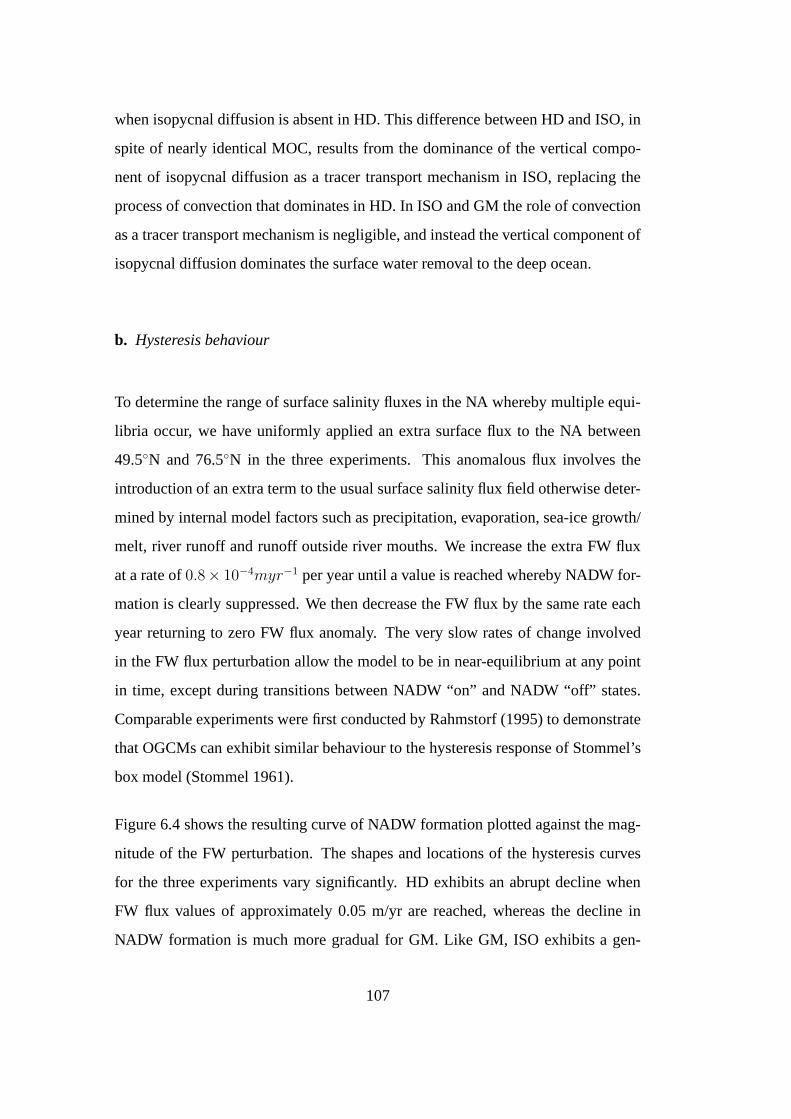
when isopycnal diffusion is absent in HD. This difference between HD and ISO, in
spite of nearly identical MOC, results from the dominance of the vertical compo-
nent of isopycnal diffusion as a tracer transport mechanism in ISO, replacing the
process of convection that dominates in HD. In ISO and GM the role of convection
as a tracer transport mechanism is negligible, and instead the vertical component of
isopycnal diffusion dominates the surface water removal to the deep ocean.
b. Hysteresis behaviour
To determine the range of surface salinity fluxes in the NA whereby multiple equi-
libria occur, we have uniformly applied an extra surface flux to the NA between
49.5◦N and 76.5◦N in the three experiments. This anomalous flux involves the
introduction of an extra term to the usual surface salinity flux field otherwise deter-
mined by internal model factors such as precipitation, evaporation, sea-ice growth/
melt, river runoff and runoff outside river mouths. We increase the extra FW flux
at a rate of 0.8× 10⁻⁴myr−1 per year until a value is reached whereby NADW for-
mation is clearly suppressed. We then decrease the FW flux by the same rate each
year returning to zero FW flux anomaly. The very slow rates of change involved
in the FW flux perturbation allow the model to be in near-equilibrium at any point
in time, except during transitions between NADW “on” and NADW “off” states.
Comparable experiments were first conducted by Rahmstorf (1995) to demonstrate
that OGCMs can exhibit similar behaviour to the hysteresis response of Stommel’s
box model (Stommel 1961).
Figure 6.4 shows the resulting curve of NADW formation plotted against the mag-
nitude of the FW perturbation. The shapes and locations of the hysteresis curves
for the three experiments vary significantly. HD exhibits an abrupt decline when
FW flux values of approximately 0.05 m/yr are reached, whereas the decline in
NADW formation is much more gradual for GM. Like GM, ISO exhibits a gen-
107

erally gradual decline in NADW during the FW addition phase, although a more
rapid decrease is simulated once NADW formation drops to below ∼ 12 Sv. The
steep decline when FW addition is at ∼ 0.05 m/yr for HD stands in contrast to GM,
wherein a stable NADW “on” state appears to persist to 0.1 m/yr. This indicates a
significantly greater NADW stability in the GM experiment. The ISO run also ex-
hibits an increased stability as as compared to HD. This suggests that the range of
FW fluxes that allow multiple equilibria is shifted in the positive direction for GM
and ISO when compared to HD. The hysteresis experiments also show that ISO and
GM maintain NADW production for FW perturbations far beyond those seen under
HD.
To further examine the stability of certain points on the hysteresis curve, we have
continued the integration for a range of constant FW flux values for several thou-
sands years of model time. Table 6.1 shows the equilibrium NADW formation rates
for HD and GM under several constant FW perturbations. For HD a constant FW
perturbation of 0.045 m/yr yields a stable NADW overturning of 20.3 Sv, whereas
a collapse is observed when 0.050 m/yr is applied. Therefore, the threshold for
NADW collapse must lie somewhere between 0.045 m/yr and 0.050 m/yr. In con-
trast, under a significantly stronger constant perturbation of 0.100 m/yr, GM permits
an “on” state of 11.5 Sv. This perturbation is more than double the FW flux that
sees HD maintain a single steady-state with no NADW formation. This indicates
that NADW is significantly more robust to the addition of FW perturbations in GM
compared to HD. Furthermore, ISO also admits a stable NADW “on” state (∼ 18
Sv) under a perturbation of 0.1 m/yr. These results confirm that NADW exhibits a
markedly increased stability to FW addition under GM and ISO compared to HD.
In summary, model experiments employing HD are much more vulnerable to a FW-
induced NADW shutdown compared to ISO and GM experiments. Equivalently,
GM and ISO experiments exhibit a greater resilience in NADW to FW perturba-
tions. We will now examine the underlying physics of this fundamental difference
108

in model behaviour.
c. Transient FW pulse experiments
To further examine the increased stability of NADW in ISO and GM, we undertake
a new set of experiments wherein a short FW pulse is applied. The magnitude of the
FW pulse (Figure 6.5 (c)) is chosen to excite a transition to a NADW “off” state.
Similar to the fluxes used in the hysteresis experiments, this is a “non-internal”
FW flux, applied uniformly in the NA between 49.5 ◦N and 76.5 ◦N. However, the
perturbation timescale of 300 years is much shorter and the model is not in near-
equilibrium during this run. Note that the maximum magnitude of the flux is also
significantly larger than that used in the hysteresis experiments, as larger values are
required to shut down NADW when a short pulse is applied due to the inertia in
the response of the system. Figure 6.5 (a) shows NADW production rate vs. time
for HD, ISO and GM. In terms of NADW production, GM and ISO recover from
an initial reduction, whereas in HD a permanent transition to a NADW “off” state
occurs in response to the perturbation. We will see that it is also possible to obtain
this stable “off” state for HD by employing even weaker perturbations than the one
shown here.
Figure 6.5 (b) shows the yearly maximum of convection depth in the North Atlantic
vs. time for HD, ISO and GM in response to the FW pulse of Fig. 6.5 (c) . The HD
run, where a transition to an “off” state occurs, exhibits an initial sharp reduction in
maximum convection depth from ∼ 2400 m depth to ∼ 200 m depth, followed by
a weak recovery to a shallow depth of less than 1000 m. The ISO run also shows a
sharp drop from similar values of ∼ 2400 m depth to around ∼ 1000 m, yet a grad-
ual recovery to the initial values of ∼ 2400 m depth occurs after the FW perturbation
has ceased. Note that although convection depth for HD and ISO are similar, the
convective transport of dye tracer is weak in ISO (see Section 6.4a). The time be-
109

haviour of convection is again different for the GM run, where no significant change
in maximum convection depth occurs in response to the perturbation for the entire
600 years. This indicates that convection does not play a significant role in the for-
mation of NADW in GM, with the convection depth remaining shallow (∼1000m)
throughout this run (even when NADW formation rates have weakened). This is in
agreement with earlier results (Sørensen et al. 2001) showing that convection is not
a significant open-ocean vertical tracer transport mechanism in models employing
a GM parametrisation of subgrid-scale eddies. The initial horizontal distribution of
convection depth in ISO is nearly identical to HD as seen in Hirst and Cai (1994)
(figure not shown). This is due to the similar density distributions for ISO and HD.
In contrast, convection depth is usually shallow and occurs over much smaller ar-
eas in models employing the GM parametrisation (e.g. Danabasoglu et al. 1994;
England 1995; Rahmstorf and Willebrand 1995) due to the increased stratification
caused by the GM parametrisation. The increased density stratification arises as
downslope flows of dense water are little mixed compared to HD and ISO exper-
iments, and in addition NADW penetration is more shallow. The representation
of convection in the Southern Ocean for GM is generally in better agreement with
observations (England and Rahmstorf 1999). It is finally noted that although HD
and ISO have similar deep NA maximum convection (∼ 2400 m, see Figure 6.5
(b)), convective tracer transport is significant in HD, yet weak in ISO. This is be-
cause the Redi (1982) isopycnal mixing terms diffuse tracers along steeply-sloping
density surfaces prior to the convection loop in the GFDL MOM.
To examine the sensitivity of NADW formation with respect to FW pulses applied to
the North Atlantic, we have conducted further experiments with FW perturbations
of identical duration and shape, but with different magnitudes. These additional
FW pulse experiments are applied to the HD and GM equilibria. Figure 6.6 shows
NADW production rate vs. time for (a) HD using perturbations attaining a maxi-
mum value of 0.34 m/yr, 0.38 m/yr, and 0.43 m/yr and (b) GM using perturbations
attaining a maximum value of 0.51 m/yr, 0.85 m/yr and 1.02 m/yr. Also shown is
110

the NADW production rate under GM employing a weak flux adjustment term of
0.06 m/yr applied to the NA concurrent with a superimposed FW pulse attaining
a maximum value of 1.53 m/yr. A slow recovery to an “on” state occurs in HD
for the perturbation peaking at 0.34 m/yr. We have verified that NADW formation
fully recovers in this experiment after more than 3000 years, whereas perturbations
peaking at values of 0.38 m/yr or greater cause a collapse of the NADW formation
when HD is used. In contrast, GM exhibits a robust response to a perturbation of
peak value 0.51 m/yr. This value is significantly higher than values whereby we
observe a collapse for HD (e.g. 0.38 m/yr). No transition to an “off” state is ob-
served with a peak perturbation of 0.51 myr−1 under GM with NADW formation
only briefly suppressed to 6-7 Sv, and within 1000 yrs a complete recovery of the
NADW “on” state is obtained. A deeper suppression of NADW and a longer recov-
ery time is observed for the strong perturbations with peak values of 0.85 m/yr and
1.02 m/yr under GM. In order to obtain a stable NADW “off” state in response to
FW forcing, we have run GM to steady state whilst applying a constant background
FW flux adjustment of 0.06 m/yr (0.02 Sv) applied to the NA (compensated by a
FW extraction of 0.02 Sv from the high latitudes of the Southern Ocean). The fixed
background FW flux is applied to ensure the possibility of a stable NADW “off”
state in GM and represents only a slight modification to the model’s hydrological
cycle. We see from Figure 6.6 that subsequent superimposition of a FW pulse at-
taining a maximum value of 1.53 m/yr (0.47 Sv, red) yields a transition to a stable
NADW “off” state by about year 600.
To examine the effect of the location of our chosen FW perturbation, we have run
an additional set of experiments similar to those shown in Figure 6.6, but applying
a FW flux to a surface area of similar spatial extent, located further to the south
at 32.4◦N - 46.6◦N (Figure not shown). We find similar behaviour to that of the
experiments described above, indicating that our FW pulse results are not depen-
dent on application of the FW anomaly over the region of convection and deepwater
formation. In the case of the subtropical-midlatitude anomalies, the models’ advec-
111

tion field moves the FW anomaly northward to the regions of deep water formation,
resulting in collapsed or sustained NADW according to choice of model mixing
scheme.
d. Diagnosis of model processes
In order to examine the roles of convection and isopycnal diffusion in driving the
dynamical behaviour of NADW sinking in response to a FW pulse we have con-
ducted additional experiments similar to the diagnostic passive tracer experiments
used to construct Figure 6.3. In particular, concurrent with applying the FW pulse
of Figure 6.5c we carry an additional passive tracer, initially zero everywhere, and
forced with a tracer flux identical in magnitude and timing to that of the FW pulse.
This allows us to “tag” the FW flux into the NA and trace its propagation through
the model, separate from its effects on salinity.
Figure 6.7 shows the yearly and volume averaged dye tracer concentration T com-
puted directly in the model for HD, ISO and GM. The decomposed budget terms
(see section 6.4a) are also shown for HD, ISO and GM. Comparing the surface
concentration of passive tracer T in the FW pulse experiments (Figure 6.7a) with
that in the NADW “on” states (Figure 6.3a) shows that the dye concentrations are
generally higher during the FW pulse experiments, indicating a reduced removal
rate of dye from the NA when FW is added and NADW formation weakens. T ′
conv
no longer dominates in HD and is negligible in ISO and GM. Figure 6.7 (b) - (d)
show that fixed background vertical diffusion (T ′
KV ) and horizontal processes (T ′
hor)
become important surface tracer removal mechanisms in the FW perturbation ex-
periments. This is related to the higher dye tracer concentrations in these experi-
ments as NADW production slows. The FW pulse causes a significant reduction in
convection for HD (Figure 6.7b). In contrast, weaker reductions occur in T ′
iso under
ISO and GM. The overall reduction of tracer transport by these previously effi-
112

cient tracer removal mechanisms (as seen in Figure 6.3) contributes to the higher
dye tracer concentrations seen during the FW pulse experiments. An accumulation
of NA dye tracer concentrations causes an increased throughput of tracer by the
previously less effective removal mechanisms, such as horizontal processes (T ′
hor)
and fixed background vertical diffusion (T ′
KV ). The strength of these processes in-
creases with increased vertical and horizontal tracer gradients resulting from the
higher concentrations at the source regions.
Another significant contributing factor to the higher surface tracer concentration in
the FW pulse experiments is the positive sign of the vertical advective tracer trans-
port T ′
w. The total vertical advection tracer fluxes were small, but negative, in the
NADW “on” set of experiments (Figure 6.3b-d). Under FW forcing, vertical advec-
tion goes from being a weak tracer removal process, to being a process that returns
tracer to the surface at 49.5◦N - 76.5◦N. This net return of dye tracer to the source
region by vertical advection arises from large areas of upward velocity at the base
of the grid cells in the surface layer within our diagnostic area. Figure 6.8 shows the
vertical velocity w for Experiment HD (NADW “on”) at the surface and at 1100m
depth. At the surface, a broad area of upwelling occurs within the diagnostic area
for the tracer budget, with downwelling occurring at the surface along the coasts
of Greenland and Northern Europe, and in parts of the Labrador Sea. At 1100m
depth, in contrast, downwelling near the Greenland coast and in the Labrador Sea
dominates. Advective tracer fluxes across the bottom interface of the surface cells
are calculated by multiplying the tracer concentration by the vertical velocity across
the interface. Since the dye tracer concentration is greater than or equal to zero, the
flux and vertical velocity are of the same sign.
To further this analysis of vertical advection in the models, table 6.2 shows the
yearly averaged rate of dye concentration change at year 200 due to vertical ad-
vection (T ′
w) and the total contributions by upward advection (T ′
up) and downward
advection (T ′
down). Also shown are the average vertical velocity (w) over the sur-
113

face slab, the average downward velocity (wdown) and the average upward velocity
(wup) at the base of the surface layer in our budget region, as well as the corre-
sponding mean tracer concentrations at the surface NA for reference. A positive
velocity w indicates upward motion. Downward velocity can be seen to be reduced
due to the increased buoyancy of surface water resulting from the FW perturbation
in HD. Counter intuitively, downward advective dye transport (T ′
down) increases in
HD when NADW is suppressed. This occurs as despite the reduction in downward
velocity, the higher surface tracer concentration results in an increase in downward
advective transport, as this transport equals the product of vertical velocity and dye
concentration. Upward advective dye transport (T ′
up) also increases due to higher
tracer concentrations (T ), as well as increased upward velocity (wup) in HD. The
magnitude of this change in upward advection is larger than the change in down-
ward advection and thus the sign of T ′
w changes in HD as FW is added. The positive
contribution of T ′
w when NADW formation is suppressed in HD therefore results
from an increase in upward advection despite downward tracer fluxes increasing.
Unlike HD, GM exhibits a reduction in downward advection that coincides with a
reduction in downward velocity, despite higher dye concentrations when NADW
is suppressed. Also, despite a slight increase in mean upward velocity and higher
mean dye concentrations, net upward advection is slightly reduced when NADW is
suppressed in GM (this can occur as the net advection is the area-weighted integral
of wT over the diagnostic domain). The increase in T ′
w therefore results solely from
a decrease in downward advection, thus allowing the upward advection to dominate.
Note that the average vertical velocity in the surface layer is upward in our diag-
nostic domain, whether or not NADW is suppressed. At first this appears contrary
to the notion of meridional overturning in the NA, although Figure 6.2 confirms
that very little (if any) of the NA overturning occurs out of the surface layer in our
diagnostic domain (49.5◦N -76.5◦N). At deeper levels, e.g. 1100 m depth, the net
vertical velocity is downward and of significant magnitude. This is in agreement
with the meridional streamfunctions shown in Figure 6.2, where a net downward
mass transport occurs at 50-70◦N, but not necessarily at the surface.
114

To compare the relative importance of the tracer transport mechanisms in the FW
perturbed (Figure 6.7) and NADW “on” states, we integrate the contributions of
the tracer transport mechanisms to T ′ by each mechanism over the first 600 years
of the model runs. Figures 6.3 (a) and 6.7 (a) show that after 600 years most of
the dye tracer has been removed from the source region. Indeed, the sum of the
time-integrated removal mechanism terms is within 2 percent of the total amount
of dye added to the ocean, indicating that only a small amount of tracer remains
in the source region after 600 years. The bar charts shown in Figure 6.9 show the
breakdown of the total amount of dye tracer removed from the surface ocean due
to convection, vertical and isopycnal diffusion, all horizontal transport processes
combined, and vertical advection (including GM where appropriate). When NADW
is “on” in the HD experiments, most dye tracer is removed by convection with only
small contributions from Thor and Tw and a slightly larger contribution from TKV
(Figure 6.9a). The maximum FW pulse HD run shows a significant reduction in
the total amount of tracer removed by convection (Figure 6.9b). This is because the
maximum convection depth decreases in response to the FW pulse (Figure 6.5b), so
that even in the isolated areas where convection is still removing surface tracer, it is
only doing so to intermediate and shallow depths. As such, the residual convective
transport shown in Figures 6.7 and 6.9 for HD only indicates transport to shallow
model layers. Once convection is weakened by the FW pulse, it is up to horizontal
advection, vertical mixing, and the downwelling component of vertical advection
to remove the surface tracer.
Experiments ISO and GM show similar differences between the NADW “on” and
FW pulse experiments. Advection is apparent in the FW pulse cases, with increased
(negative) horizontal transport offset in part (ISO) or fully (GM) by positive verti-
cal transport. In contrast, advection effects are relatively small in the steady NADW
“on” version of these experiments, although horizontal and vertical advection ap-
pear to play a non-negligible role in the GM run, perhaps due to the GM advective
terms. Tracer removal by convection is very weak for the NADW “on” states of ISO
115

and GM, and even smaller for the FW pulse versions. Instead, isopycnal diffusion
(T ′
iso) takes the place of convection as the dominating tracer removal process for
ISO and GM in the NADW “on” experiments. This is due to the vertical compo-
nent of isopycnal diffusion arising from sloping density surfaces in the NA. Most
importantly, removal of tracer by isopycnal mixing is not substantially weakened in
the FW pulse experiments (Figure 6.9b), particularly in GM, in stark contrast to the
convection collapse in HD.
6.5. Discussion and Conclusions
We have shown that replacement of fixed horizontal diffusion by the GM parametri-
sation in a coupled model strongly increases its stability with respect to an anoma-
lous FW pulse applied to the NA. When we first made this discovery, our initial
hypothesis was that a reduction in the “Veronis effect” under GM (e.g. B oning
et al. 1995) lead to an increased capacity for FW export from the NA, reducing
the sensitivity of NADW to FW pulses in the region. Under this hypothesis, HD
experiments are vulnerable to a freshwater-induced NADW collapse as the Vero-
nis effect recycles water in a shallow cell within the North Atlantic. However, dye
tracer experiments in the North Atlantic disproved this hypothesis. Instead we find
isopycnal diffusion to be the cause of the increased NADW formation stability with
respect to FW addition in our experiments.
Our hysteresis experiments show that the increased stability of the GM run is as-
sociated with an increased NADW stability with respect to constant external NA
FW addition (see Figure 6.4 and Table 6.1). The difference in behaviour between
GM and HD in response to short FW pulses is therefore not a feature arising from
transient dynamical factors, but relates to the actual existence of multiple equilib-
ria. The significant increase in NADW stability upon the introduction of isopycnal
diffusion seen in the ISO experiments indicates that isopycnal diffusion of tracer,
116

rather than isopycnal thickness diffusion, is responsible for the increased NADW
stability observed in the GM run. This result is robust with respect to the choice
of isopycnal diffusion rates (we have tested values at half and one quarter of that
reported above). Also, the NADW behaviour in the ISO run shows that the fixed
background horizontal diffusivity is not in itself responsible for reducing NADW
stability in the HD run. Indeed, despite the very similar density distribution and
overturning of HD and ISO when a FW pulse is applied, the dynamical responses
to FW addition are very different under these two mixing parametrisations.
Our HD budget analysis shows that in the NADW sinking regions, convection is
the dominant mechanism whereby vertical tracer transport into the ocean’s interior
occurs. In contrast, in ISO this role is replaced by isopycnal diffusion. Under FW
forcing, the reduction in vertical tracer transport by isopycnal diffusion in ISO is
not as large as the reduction of convection in HD. Also, the recovery of NADW
formation in ISO indicates a stronger capacity for re-establishment of this transport
mechanism after its reduction by a surface anomaly of FW. Even less reduction
of isopycnal diffusion occurs in GM, implying a stronger insensitivity of NADW
sinking to FW perturbations compared to ISO. This is borne out by the NADW
formation rate behaviour shown in the hysteresis experiments (Figure 6.4) and the
FW pulse experiments (Figure 6.5). The ability of isopycnal diffusion to remain
present during a FW perturbation in ISO and GM, albeit along less-steeply sloped
density surfaces, appears to be the key factor in the increased stability of NADW
formation seen in our series of experiments.
The decreased tendency of NADW to collapse in response to an anomalous surface
FW flux when isopycnal diffusivity is employed derives from the increased robust-
ness of the vertical component of isopycnal diffusivity over convection as a vertical
tracer transport mechanism. This increased insensitivity is due to the fact that the
vertical isopycnal transport can mix FW along density surfaces into the ocean inte-
rior, whereas convection only operates on unstably stratified columns. The stronger
117

precondition for convection to occur is more easily removed by the application of
a FW perturbation. The weakening of convection in response to FW addition are
illustrated by the precipitous decline of maximum convection depth seen in Fig-
ure 6.5 (b). Application of the FW pulse results in a significant shoaling of the
depth range of static instability associated with winter surface cooling in HD. Per-
sistent isopycnal transports from the NA surface into the ocean interior, in contrast,
can occur under stably stratified conditions. The isopycnal mixing process contin-
ues to operate during the addition of a FW pulse, whereas convection shuts down.
This is most strongly borne out by our tracer budget for the GM run, where signifi-
cant tracer transport by the vertical component of isopycnal diffusion persists while
the FW perturbation is applied. The hysteresis experiments show that despite the
increased NADW stability in GM and ISO, NADW “off” states do occur for a range
of FW flux values (at notably higher rates than those required to collapse NADW in
HD). In this case surface density in the NA is reduced, so that the deep isopycnals
associated with NADW no longer outcrop at the surface. Instead, shallow tracer
penetration occurs by isopycnal diffusion and deep water formation is absent. To
summarise our results, Figure 6.10 shows a schematic diagram of NADW formation
sensitivity to vertical tracer removal processes.
It is noted that although the GM parametrisation represents a more realistic repre-
sentation of the effect of mesoscale eddies on tracers in ocean models, our results
do not necessarily imply that greater realism of NADW stability is attained under
GM. Rather, we have highlighted an undesirable sensitivity of NADW stability to
choice of mixing scheme. Care ought to be taken when seeking to obtain critical
thresholds for FW-induced collapse of NADW in ocean and coupled climate mod-
els as the required FW rates are set, in part, by the choice of model mixing scheme.
Since the surface area where we apply the FW flux is relatively large, targeting the
FW perturbation directly over the Labrador Sea convection area (as was done, for
example, in Rahmstorf 1995), would see an even lower threshold for NADW col-
lapse under HD. Our study suggests a dramatically different FW threshold would
118

exist under GM in such experiments.
Deep water formation in the real ocean occurs via processes that remain unresolved
in coarse resolution global OGCMs. In the real ocean, convection in the North At-
lantic may collapse in response to a decrease in surface density arising from fresh-
ening due to increased melt water or enhanced precipitation (Manabe and Stouffer
1994), heating from above (Mikolajewicz and Voss 2000) or a freshening followed
by warming (Bi et al. 2001). Modelling studies have also shown a prolonged sup-
pression of AABW in coupled climate models (e.g. Bi et al. 2002, 2001) in response
to increased CO2 forcing. We have demonstrated that in ocean models, NADW
stability depends on the choice of model mixing scheme. The increased stability
of NADW formation to FW perturbations under ISO and GM point to the impor-
tance of further study into the respresentation of deep water formation processes in
OGCMs. In particular, it remains unclear whether or not the degree of isopycnal
diffusion simulated in ocean models is realistic. Direct observations of this process
are limited, as is our knowledge of the appropriate coefficient to use for along-
isopycnal diffusion in ocean models. Our study suggests that NADW formation in
ocean models employing GM may be more stable with respect to FW perturbations
than is suggested on the basis of convection alone. Conversely, if isopycnal mixing
is over-estimated in ocean models or if it is unrealistically represented, a refinement
of this parametrisation is required.
119

Table 6.1: Equilibrium NADW formation for HD and GM under several constant
perturbations applied over a period of several thousand years. Magnitudes of the
perturbations are shown in column 2 and NADW formation rate, if applicable, is
listed in column 3. A dash (-) indicates the absence of a stable NADW “on” state.
Experiment Perturbarion (m/yr) NADW (Sv) State
HD 0.045 20.2 NADW ”on”
HD 0.05 - NADW ”off”
GM 0.1 11.5 NADW ”on”
ISO 0.1 18.0 NADW ”on”
120

Table 6.2: Yearly average of rate of change of spatially averaged dye concentration
at year 200 due to vertical advection (T ′
w), upwelling (T ′
up) and downwelling (T ′
down)
at the surface layer. Note that net vertical transport by advection equals the sum of
the upwelling and downwelling components. Also shown are the yearly average
at year 200 of vertical velocity (w), upwelling (wup) downwelling (wdown) in 10−7
m/s. Also shown are the yearly averaged values of tracer concentration T (ppt)
in the surface layer at year 200. Values are volume-averaged over the upper 50
m of the North Atlantic between 49.5 ◦N and 76.5 ◦N. Negative values indicate
downward fluxes and velocities, respectively.
Experiment T′
w(m
/yr)
T′
up(m
/yr)
T′
dow
n(m
/yr)
w(1
0−
7
m/s
)
wup,(1
0−
7
m/s
)
wdo
wn
(10−
7
m/s
)
T(p
pt)
GM (FW pulse) 0.25 2.02 -1.77 2.65 7.77 -5.12 2.01
HD (FW pulse) 0.20 1.05 -0.85 2.61 7.38 -4.77 2.05
GM (NADW “on”) -0.06 2.07 -2.13 1.35 7.12 -5.78 1.74
HD (NADW “on”) -0.03 0.41 -0.44 0.67 7.05 -6.38 1.22
121

76.5 N
50m
49.5 N
isopycnal
FISO
Fconv
FKv
FHOR
FW
T
ATLANTIC
FSURFACE
NEQ
Figure 6.1: Schematic representation of tracer removal mechanisms in the model.
The tracer flux into the North Atlantic surface region (stippled) is denoted by
Fsurface. The fluxes Fhor (all horizontal processes including GM), FKV(vertical
mixing), FISO (isopycnal mixing), Fconv (convection) and Fw (vertical velocity, in-
cluding GM velocity) act to remove or return tracer from the surface region.
122

4
3
2
1
DE
PT
H (
km)
0
0
00
0
0
0
2018161412108642
−2−4
−4
−2
121062
(a) HD
4
3
2
1
DE
PT
H (
km)
00 0
0
20181614
1012
86
42−2
−4
−2
10862
10
2
(b) ISO
30S EQ 30N 60N
4
3
2
1
LATITUDE
DE
PT
H (
km)
0
0
0
0
0
0
1412108
642
−2−4−4
−2
−4
62
84
(c) GM
Figure 6.2: Atlantic meridional overturning streamfunction (10 year average) for
steady “NADW on” states in (a) HD, (b) ISO and (c) GM. Values are given in Sv
(1 Sv = 106 m3 sec−1).
123

0
0.5
1
1.5
2
2.5
ppt
(a) Dye concentration T
−0.4−0.3−0.2−0.1
00.10.20.30.4
FLU
X (
m/y
r)
(b) HD
−0.4−0.3−0.2−0.1
00.10.20.30.4
FLU
X (
m/y
r)
(c) ISO
−0.4−0.3−0.2−0.1
00.10.20.30.4
FLU
X (
m/y
r)
(d) GM
convisoK
V
horizw
HDISOGM
0 100 200 300 400 500 6000
0.5
TIME (year)
FLU
X (
m/y
r) (e) Dye flux
Figure 6.3: (a) Time series of volume averaged dye tracer concentration T in HD,
ISO and GM in the North Atlantic in response to the dye fluxes indicated in Figure
6.3e in the steady state NADW “on” experiments. Values are volume averaged
over the upper 50 m of the North Atlantic between 49.5 ◦N and 76.5 ◦N. Units are
in parts per thousand for comparison with the FW pulse experiments of Fig. 6.7.
(b)-(d) Time rate of change of volume averaged dye tracer concentration due to
convection (blue), isopycnal diffusion (black), fixed background vertical diffusivity
Kv (green), horizontal diffusion and advection including the horizontal component
of isopycnal diffusion and GM velocities (red) and vertical velocity including GM
velocity (cyan). Shown are results for experiments (b) HD, (c) ISO, (d) GM.
124

0 0.05 0.1 0.15 0.2 0.25 0.30
5
10
15
20
25
FW Flux (m/yr)
NA
DW
(S
V)
HDISOGM
0 1.5 3.0 4.5 6.0 7.5
FW Flux (10−2 Sv)
Figure 6.4: Hysteresis behaviour of NADW sinking rate in response to FW flux
anomalies applied in the North Atlantic for HD (bold), ISO (dashed) and GM (stip-
pled). The FW flux anomaly is compensated by a flux anomaly of equal magnitude
and opposite sign applied to the high latitudes of the Southern Ocean. The NADW
formation rate (vertical axis, in Sv) is plotted against the FW perturbation rate (bot-
tom horizontal axis, in m/yr). The equivalent FW flux in Sv is displayed along the
top axis (1 Sv = 106 m3 sec−1).
125

0
5
10
15
20
Sv
(a) NADW production
0
0.5
1
1.5
2
2.5
DE
PT
H (
km)
(b) Convection depth
0 100 200 300 400 500 6000
0.5
TIME (year)
m/y
r
(c) FW flux
HDISOGM
Figure 6.5: (a) NADW production rate vs. time for HD (solid), ISO (dashed) and
GM (dotted) in response to a FW perturbation. (b) Yearly maximum of convection
depth (m) in the North Atlantic vs. time for HD (solid), ISO (dashed) and GM
(dotted). (c) Time history of the FW perturbation applied to the North Atlantic
between 49.5 ◦N and 76.5 ◦N.
126

0
5
10
15
20
25
Sv
(a) HD
0 500 1000 1500 2000 25000
5
10
15
TIME (year)
Sv
(b) GM
HD 0.34 HD 0.38 HD 0.43
GM 0.51 GM 0.85 GM 1.02 GM 1.53
Figure 6.6: NADW production rate vs. time for (a) HD using perturbations attaining
a maximum value of 0.34 m/yr (0.1 Sv, blue), 0.38 m/yr (0.12 Sv, black), and 0.43
m/yr (0.13 Sv, green) and (b) GM using perturbations attaining a maximum value
of 0.51 m/yr (0.15 Sv, blue), 0.85 m/yr (0.26 Sv, black), 1.02 m/yr (0.31 Sv, green).
Also shown in (b) is the NADW production rate in GM with a constant background
FW flux adjustment term of 0.06 m/yr (0.02 Sv) applied to the NA concurrent with
a superimposed FW pulse attaining a maximum value of 1.53 m/yr (0.47 Sv, red).
The NA FW perturbations are identical in shape to the perturbation curve shown
in Figure 6.5, but have different amplitudes as indicated in m/yr in the respective
legends (1 Sv = 106 m3 sec−1).
127

0
0.5
1
1.5
2
2.5
ppt
(a) Dye concentration T
−0.4
−0.3
−0.2
−0.1
0
0.1
0.2
0.3
0.4F
LUX
(m
/yr)
(b) HD
−0.4
−0.3
−0.2
−0.1
0
0.1
0.2
0.3
0.4
FLU
X (
m/y
r)
(c) ISO
0 100 200 300 400 500 600−0.4
−0.3
−0.2
−0.1
0
0.1
0.2
0.3
0.4
TIME (year)
FLU
X (
m/y
r)
(d) GM
convectiso diffK
V
horizontw
HDISOGM
Figure 6.7: Time series of dye tracer concentrations and their component time
derivatives in response to the FW perturbation indicated in Figure 6.5 (c) volume-
averaged over the upper 50 m of the North Atlantic between 49.5 ◦N and 76.5 ◦N.
The dye tracer flux is equal in magnitude to the FW flux. (a) Volume averaged
dye tracer concentration for HD (solid line), ISO (dashed) and GM (dotted). The
dye tracer can be expressed in ppt as it represents FW added to the ocean. (b)-(d)
Time rate of change of volume averaged dye tracer concentration due to convec-
tion (blue), isopycnal diffusion (black), fixed background vertical diffusivity KV
(green), horizontal diffusion and advection including the horizontal component of
isopycnal diffusion and GM velocities where appropriate (red) and vertical veloc-
ity including GM velocity where appropriate (cyan). Shown are components for
experiments (b) HD, (c) ISO, and (d) GM.
128

m/s
−5
0
5
x 10−6
m/s
−5
0
5
x 10−6
50
55
60
65
70
75
80
LAT
ITU
DE
(a) w at surface
Greenland
Europe
w= 0.7x10⁻⁷ m/s
−55 −35 −15 5 25 45
50
55
60
65
70
75
80
LONGITUDE
LAT
ITU
DE
(b) w at 1100m depth
Greenland
Europe
w= −1.9x10⁻⁶ m/s
x x x x x
x
Figure 6.8: Yearly mean of vertical velocity w (in m/s) in the North Atlantic for
HD in the NADW “on” experiment at (a) the surface and (b) 1100m depth. Positive
values indicate upward motion. The stippled lines indicate the bounding latitudes
of the region used to diagnose the tracer budget terms of Fig. 6.7. The color scale
has been set to be identical to that of (a). Downward vertical velocities in signifi-
cant excess of the lower limit of the color scale occur in the area marked “X” off
Greenland, where strong downwelling occurs. Indicated in the lower right corners
of the panels are the area-averaged velocities w in m/s.
129

−100
−80
−60
−40
−20
0
20
40
60
80
100
FW
(m
)
(a) NADW "on" states
conv iso K_v hor w−100
−80
−60
−40
−20
0
20
40
60
80
100
PROCESS
FW
(m
)
(b) FW pulse experiments
HDISOGM
Figure 6.9: Bar chart depicting a budget breakdown by process of the total amount
of dye tracer that has been removed from the NA source region during the period
between year 0 and year 600 for (a) the steady state NADW “on” runs and (b) the
FW pulse runs. HD is indicated by the solid bars, ISO by the grey bars and GM
by the white bars. For each experiment the sum of the bar values very closely
matches the total amount of tracer input over the corresponding period, indicating
that most of the tracer has been removed by year 600. The breakdown includes
convection (conv), isopycnal diffusion (iso), background vertical diffusion (KV ),
all horizontally acting tracer transport processes (hor) and advection by vertical
velocity, including the GM velocity (w).
130

No isopycnal diffusion
M OT sensitive to FFW
ATLANTIC
T
(a) HD
convection
dom inates
rem oval of tracer
FFW
M OT less sensitive to FFW
isopycnal diffusion
rem oves tracer
convection
relatively
w eak
(b) GM
T
FFW
NEQ
Figure 6.10: Schematic representation of NADW formation (curved downward
pointing arrow from the surface) and tracer removal processes responsible for its
stability with respect to a FW perturbation in (a) HD and (b) GM. The surface re-
gion where a FW flux is applied is indicated by the stippled box and tracer concen-
tration by T. Convection is much more sensitive to a FW perturbation than isopycnal
diffusion, yielding more stable NADW in GM experiments.
131

Chapter 7
Sensitivity of the Atlantic
thermohaline circulation to
basin-scale variations in vertical
mixing and its stability to fresh water
perturbations
7.1. Abstract
We show that a reduction in vertical mixing applied inside the Atlantic basin can
drastically increase North Antlantic Deep Water (NADW) stability with respect to
fresh water (FW) perturbations applied to the North Atlantic (NA). This is contrary
to the notion that the ocean’s meridional overturning circulation simply scales with
vertical mixing rates. An Antarctic Intermediate Water (AAIW) reverse cell, reliant
upon upwelling of cold AAIW into the Atlantic thermocline, has been previously
132

associated with stable states where NADW is collapsed and transitions between
NADW “on” and “off” states are characterised by interhemispheric competition
between this AAIW cell and the NADW cell. In contrast to the AAIW reverse cell,
NADW eventually upwells outside the Atlantic basin, and is thus not subject to the
same impediment as the AAIW reverse cell when vertical mixing is reduced inside
the Atlantic. We show that a reduction of vertical mixing in the Atlantic weakens
the AAIW reverse cell, resulting in a shift of the competition between the two cells
in favour of NADW formation. Our results suggest that the AAIW reverse cell is
responsible for the stability of NADW collapsed states, and thereby plays a key role
in maintaining multiple equilibria in the climate system.
7.2. Introduction
Stommel (1961) first proposed the possibility that the ocean’s thermohaline circu-
lation could have two stable regimes of flow. Bryan (1986) demonstrated how the
operation of a positive salt feedback could bring about two asymmetric overturn-
ing states under symmetric surface flux conditions in a rectangular basin geometry.
In his idealised model, there is competition for interhemispheric fresh water (FW)
export between two overturning cells involving the sinking of water originating at
the antipodean polar surface of the basin. The real ocean, however, contains an ob-
struction to southward geostrophic flow across the latitudes of Drake Passage, thus
inhibiting the formation of the vigorous Southern Hemisphere (SH) cell observed
by Bryan (1986). Instead, studies employing a more realistic geometry (e.g. Man-
abe and Stouffer 1988; Saenko et al. 2003; Gregory et al. 2003; Rahmstorf 1996;
Sijp and England 2005) find that SH overturning states exhibit a shallower Antarc-
tic Intermediate Water (AAIW) reverse cell inside the Atlantic basin. In contrast to
the SH cell of Bryan (1986) or studies employing a Drake Passage closed geome-
try (e.g. Mikolajewicz et al. 1993; Sijp and England 2004), this AAIW reverse cell
133

originates at the AAIW formation regions. Saenko et al. (2003) show that due to
the existence of this cell in a North Antlantic Deep Water (NADW) “off” state, the
density difference between surface waters and the formation regions for AAIW and
NADW determines the strength and polarity of the meridional overturning (MOC).
Sijp and England (2005) show that the nature of this relationship depends on the
depth of the Drake Passage, with Antarctic Bottom Water (AABW) playing a re-
duced role as the DP deepens. Furthermore, Saenko et al. (2003) and Gregory et al.
(2003) suggest that this AAIW reverse cell can contribute to maintaining a stable
NADW “off” state by importing FW into the Atlantic basin, and that it cannot co-
exist with the NADW formation cell.
In coarse resolution ocean models where vertical mixing is set to appreciable val-
ues, the upwelling branches of the NADW cell and the AAIW reverse cell rely
in part on vertical mixing at lower latitudes. This upwelling into the thermocline
consists of a balance between downward diffusion of heat from the surface and
upward advection of colder water from below the thermocline (e.g. Munk 1966;
Munk and Wunsch 1998), the balance determining the global thermocline depth.
Enhanced vertical mixing therefore increases transport in the upwelling branches
of these cells. Indeed, Bryan (1987) found that larger vertical mixing rates lead to
increased MOC in an idealised sector geometry model. There have been several
other studies that investigate the role of vertical mixing in setting the thermohaline
circulation (THC) strength in global ocean climate models. Manabe and Stouffer
(1999) showed that the stability of their NADW “off” state depends on the value
of vertical mixing. Studies employing a zonally averaged model (Schmittner and
Weaver 2001) and a three dimensional ocean model (Prange et al. 2003) use hys-
teresis experiments to show that the stability of the NADW “off” and “on” states
depend on the rate of vertical mixing. These studies, however, employ horizontally
uniform vertical mixing. In our study, we assess the sensitivity of the THC with
respect to basin-wide changes in Kv. In particular, we examine the effect of a re-
duction in vertical mixing inside the Atlantic on the stability of NADW formation
134

with respect to FW perturbations applied to the NADW formation regions.
The AAIW reverse cell of the NADW “off” state relies on upwelling inside the At-
lantic basin, whereas in the NADW “on” state, NADW outflow leaves the Atlantic
basin at 30◦S to upwell outside this basin. Broecker (1991) highlights the role of
the Indian and Pacific Oceans in the removal of NADW by vertical mixing at low
latitudes in the classical “global ocean conveyor belt” schematic. Later studies (e.g.
Toggweiler and Samuels 1995) suggest instead that a significant portion of NADW
resurfaces via wind-driven upwelling in the Southern Ocean and undergoes sub-
sequent buoyancy changes due to surface fluxes. Model studies employing weak
background vertical mixing also support this (e.g. Saenko and Merryfield 2005).
As the upwelling branches of the NADW cell and the AAIW reverse cell occur
at different locations, the spatial distribution of vertical mixing in the world ocean
may affect the relative potential of these cells for dominance of deep ocean venti-
lation. In particular, the AAIW reverse cell relies upon the removal of intermediate
water across the Atlantic thermocline via diapycnal mixing. Hence, a reduction in
vertical mixing at low latitudes of the Atlantic should reduce the strength of the
AAIW reverse cell and therefore its ability to compete with NADW. The NADW
cell, on the other hand, does not rely on Atlantic upwelling and may therefore be
less sensitive to a reduction in vertical mixing inside the Atlantic. In this situation,
a greater robustness of NADW overturning with respect to FW perturbations may
ensue. In this study, we use a coupled climate model to examine the stability of
NADW formation under different spatial distributions of vertical mixing.
The remainder of this note is divided as follows. Section 7.3 covers a description of
the model and experimental design. We will consider three main experiments, the
first with a reduced vertical mixing coefficient (Kv) inside the Atlantic Ocean, the
second employing a reduced Kv inside the Indian and Pacific Oceans, and the third
being a control experiment wherein Kv is not reduced. In section 7.4 we discuss
the steady state fields under the three different vertical mixing scenarios, and their
135

response to the application of external FW flux pulses. Finally, section 7.5 covers a
discussion and conclusions.
7.3. Model and Numerical Experiments
The simulations have been carried out using the Earth System Climate Model of
intermediate complexity of Weaver et al. (2001) described in Chapter 2. Here, we
use version 2.6. For economy of computation, with many multi-millennial integra-
tions, no parametrisation of along isopycnal diffusion (Redi 1982) or eddy-induced
advective tracer transport (Gent and McWilliams 1990) is used in the standard set
of experiments. Rather, our focus is on model THC sensitivity to vertical diffusive
mixing. It is noted, however, that we re-evaluated several of the experiments under
GM and confirm that our results are robust in both GM and non-GM experiments.
To examine the effect of reducing Kv in different ocean basins, we have integrated
three main configurations of the model to equilibrium: (1) a control experiment
CNTRL, where no reduction in Kv is applied, (2) an experiment where Kv is re-
duced inside the Atlantic basin, denoted 1
3KVAtl, and (3) an experiment where Kv
is reduced inside the Pacific and Indian basin, denoted 1
3KVIP . This reduction by a
factor of 1/3 is only applied between the surface and 1257 m depth, with no change
in Kv at levels deeper than 1257 m. The reduction is also only applied between
35◦S and 48◦N in each ocean basin. In addition to these three main experiments,
we have also run a series of auxiliary experiments where Kv is reduced by a range of
factors to test the robustness of our results. Values of 3/4, 2/3 and 1/2 were tested.
A version of 1
3KVAtl using GM has also been run to verify the robustness of our
results with respect to the choice parametrization of subgrid scale turbulent mixing
of tracer properties.
The ocean exhibits substantial regional variations in Kv (e.g. Ledwell et al. 2000),
136

thought to be a function of tidal currents, subsurface bathymetry and local strat-
ification. Several studies have examined the effects of locally enhanced vertical
diffusivity over rough bathymetry in ocean models (e.g. Hasumi and Suginohara
1999; Saenko and Merryfield 2005). Unlike these previous studies, we make no at-
tempt to examine the effects of contrasts in vertical mixing that may exist between
basins in the real ocean. Instead our experiments are specifically aimed to examine
the role of the location of deepwater removal in determining the global THC and its
stability.
Figure 7.1 (a) shows the two areas where reduction of Kv is applied in 1
3KVAtl
and 1
3KVIP . To the model equilibria we then apply FW perturbations of different
magnitude in the NA to examine transitions between NADW “off” and NADW “on”
states. These perturbations are applied in the NA between the dashed black lines
shown in Figure 7.1 (a). Figure 7.1 (b) shows the FW perturbation against time.
A linear increase from 0 to a maximum value M occurs over the first 150 years,
followed by a linear decline back to 0 over the following 150 years. After year
300, no further FW perturbation is applied. This procedure, similar to that of Sijp
and England (2005), is designed to examine the existence of multiple equilibria in
the experiments. The value of M varies over a series of experiments as described
below.
7.4. Results
Figure 7.2 shows the MOC in the Atlantic basin for (a) the NADW “on” CNTRL
state, (b) the NADW “off” CNTRL state and (c) the NADW “off” state for aux-
iliary experiment 2
3KVAtl, where Kv is reduced by a factor of 2/3 in the Atlantic.
The NADW “on” state exhibits 20 Sv of NADW formation (1 Sv = 106 m3 sec−1);
throughout this paper all transport values are quoted to the nearest 1 Sv). The CN-
TRL NADW “off” state was obtained from the NADW “on” state by applying a
137

perturbation of maximum value M=0.38 m/ yr. This NADW “off” state exhibits an
AAIW reverse cell of 9 Sv. This cell overlies an Antarctic Bottom Water (AABW)
cell recirculating below 2000m depth with an AABW inflow of 4 Sv. In the aux-
iliary experiment 2
3KVAtl (Fig. 7.2 c) the AAIW reverse cell is reduced by 3 Sv,
taking a value of 6 Sv, and is restricted to shallower depths. This reduction in the
strength and depth of the AAIW reverse cell results from a reduced potential for
AAIW upwelling into the Atlantic thermocline due to lower vertical mixing values
there. This result illustrates the dependence of the AAIW reverse cell on vertical
mixing inside the Atlantic basin. In contrast, the AABW recirculation in 2
3KVAtl
is similar (4 Sv) to that of the the NADW “off” state in CNTRL (4 Sv). This is
because AABW inflow into the Atlantic returns south at depth, and is not affected
by changes in vertical mixing applied in the upper 1257 m.
The auxiliary experiment 2
3KVAtl also admits a NADW “on” state (figure not shown).
The NADW “off” state described above has been obtain from the NADW “on” state
in a similar fashion to CNTRL. In contrast, it is noted that we were unable to ob-
tain stable NADW “off” states for reductions of Atlantic Kv using multiplication
factors of between 1/10 and 1/2. This is because a strong reduction in the Atlantic
weakens the AAIW reverse cell that is otherwise required to prevent the eventual
re-establishment of the NADW cell. However, reduction by the milder factor of
2/3 inside the Atlantic, as described above, allowed us to obtain a stable NADW
“off” state. The existence of this NADW “off” state in the 2
3KVAtl experiment
therefore allowed us to examine the effect of vertical mixing in the Atlantic on the
AAIW reverse cell. Higher reductions of Kv evidently reduce the strength of the
AAIW reverse cell to the extent that is unstable, and collapses to allow NADW
to re-establish. Figure 7.3 summarizes these results and shows the timeseries for
experiments 1
4KVAtl ,1
3KVAtl, 1
2KVAtl and 2
3KVAtl under a FW perturbation attain-
ing a maximum value of 1.02 m/yr after 150 years. Timeseries are shown for (a)
NADW production rate and (b) the AAIW reverse cell.
138

Figure 7.5 shows the unperturbed Atlantic MOC of (a) experiment 1
3KVAtl and (b)
experiment 1
3KVIP . For 1
3KVAtl, NADW formation is reduced from 20 Sv in CN-
TRL to 18 Sv. It is interesting to note that despite a reduction in NADW formation,
NADW outflow is increased from 12 Sv in CNTRL to 14 Sv in 1
3KVAtl. This im-
plies a reduction of NADW recirculation inside the Atlantic1 from 10 Sv in the con-
trol experiment to 4 Sv when vertical mixing is reduced in 1
3KVAtl. Thus, the rate
of NADW recirculation inside the Atlantic basin depends on the rate of localised
vertical mixing. A reduction of vertical mixing in the Atlantic therefore reduces
this recirculation, which is compensated in part by reduced NADW formation, and
in part by an increase in NADW outflow.
For 1
3KVIP (Fig. 7.5b), the Atlantic MOC is similar to that of the NADW “off” state
shown in Fig. 7.2a, with an AAIW reverse cell of 9 Sv overlying an AABW cell,
recirculating below 2000m depth with an AABW inflow of 4 Sv. This suggests that
the Atlantic circulation of the NADW “off” state in CNTRL is not significantly
influenced by vertical mixing outside the Atlantic basin. The similarity between
the CNTRL NADW “off” state and 1
3KVIP arises because the AAIW reverse cell
relies exclusively on vertical mixing inside the Atlantic for its upwelling branch.
We have tried to excite a transition to a NADW “on” state in 1
3KVIP by applying
FW pulses to the NA without success. Figure 7.4 shows the timeseries for experi-
ments 1
3KVPac under a FW perturbation attaining a maximum of 1.7 m/yr after 150
years. Timeseries are shown for (a) NADW production rate and (b) the AAIW re-
verse cell. Apparently, in our model, the Indian and Pacific oceans comprise an area
of significant deepwater removal by vertical mixing. This sensitivity of NADW to
vertical mixing inside the Indian and Pacific Oceans indicates that alternative re-
moval mechanisms, such as mechanically driven upwelling due to wind stress in
the Southern Ocean, are not sufficient alone to maintain the NADW cell in the ab-
sence of strong Indo-Pacific vertical mixing in our model. A dye tracer experiment
1We calculate this recirculation by subtracting the NADW outflow rate from the NADW forma-
tion rate
139

(figure not shown) shows upwelling of NADW in the lower latitudes of the Indian
and Pacific Oceans, as well as at some locations in the high latitudes of the Southern
Ocean. This confirms the importance of the Indian/ Pacific and Southern Oceans in
the removal of NADW from the deep oceans . Therefore, in our model, a reduc-
tion of vertical mixing inside the Indian and Pacific Oceans shifts the competitive
advantage of the AAIW/ NADW cells in favour of the AAIW cell. This result is in
agreement with Prange et al. (2003), who find a strong sensitivity of MOC to global
Kv, but relatively little sensitivity to Southern Ocean winds in their model.
Figure 7.6 shows timeseries of (a) NADW formation and (b) the AAIW reverse cell
in response to the application of a FW flux (Fig. 7.1b) in the NA for CNTRL and
1
3KVAtl. A perturbation of maximum value M=0.38 m/yr is applied to the control
experiment and yields a stable NADW “off” state (Fig. 7.6a). When FW pulses
attaining higher maximum values M of 0.51 m/ yr, 1.02 m/ yr and 1.53 m/ yr are
applied to 1
3KVAtl, NADW formation eventually recovers to a NADW “on” state
(Fig. 7.6a). The NADW shutdown in CNTRL concurs with the emergence of the
AAIW reverse cell (Fig. 7.6b), which eventually attains a value of 9 Sv. When Kv
is reduced in the Atlantic, however, the role of the AAIW reverse cell appears to
be diminished. Despite the initial suppression of the NADW cell in response to the
FW perturbations applied to 1
3KVAtl, and the temporary establishment of a higher
maximum strength AAIW reverse cell in one of the experiments, there is no perma-
nent establishment of this cell. Whilst the FW pulse is applied, NADW formation is
suppressed. This indicates that altered surface conditions at the NADW formation
regions prevent sinking during this period. After the perturbation has terminated,
however, NADW formation recovers over a period of 1500-2500 years. This indi-
cates that in the absence of an external FW flux, circulation changes alone cannot
maintain the light surface conditions at the NADW formation regions required to
prevent sinking when Kv is reduced by a factor of 1/3 in the Atlantic .
During suppression of the NADW cell in 1
3KVAtl, an AAIW reverse cell emerges
140

that is generally weaker than in CNTRL, due to the reduced ability of AAIW to
upwell into the Atlantic thermocline when vertical mixing is reduced. This AAIW
reverse cell is not stable, so it does not accomplish the FW import into the Atlantic
basin required to maintain surface conditions that prevent NH sinking. With the
consequent emergence of the NADW cell, the AAIW reverse cell is progressively
reduced in strength, culminating in its termination approximately 1200-2000 years
after initiation of the FW pulse. In contrast to the AAIW reverse cell, NADW finds
its upwelling areas outside the Atlantic basin, and is thus not subject to the same
impediment as the AAIW reverse cell in 1
3KVAtl. This indicates that a reduction of
Kv inside the Atlantic basin favours the NADW cell by inhibiting the AAIW reverse
cell.
The enhanced stability of the NADW cell in 1
3KVAtl is not the result of changes in
surface density or isotherm depth. The surface conditions in 1
3KVAtl indicate a cool-
ing and freshening of the NADW formation regions relative to CNTRL (figure not
shown), with the net effect of this change a reduction of surface density in the North
Atlantic. The lighter surface conditions in the NA in 1
3KVAtl are less favourable to
the stability of the NADW cell. This proves that changes in NA surface density
in 1
3KVAtl are not responsible for the increased stability of NADW. Furthermore,
as expected, we observe a shoaling of the isotherms in the upper 2000 m of the
Atlantic in 1
3KVAtl relative to CNTRL(figure not shown). A deepening of Atlantic
isotherms is known to enhance NADW formation (Gnanadesikan 1999) and per-
haps its stability, yet we find no significant deepening of the Atlantic isotherms in
the upper 2000 m in 1
3KVAtl. We have shown in contrast that a reduction in verti-
cal mixing inside the Atlantic with respect to the rest of the world ocean leads to
an increased stability of NADW formation. This results from the inhibition of the
AAIW reverse cell by the reduced vertical mixing in the Atlantic. A very different
picture emerges when Kv is reduced in the Indian and Pacific oceans.
141
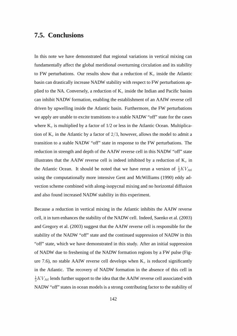
7.5. Conclusions
In this note we have demonstrated that regional variations in vertical mixing can
fundamentally affect the global meridional overturning circulation and its stability
to FW perturbations. Our results show that a reduction of Kv inside the Atlantic
basin can drastically increase NADW stability with respect to FW perturbations ap-
plied to the NA. Conversely, a reduction of Kv inside the Indian and Pacific basins
can inhibit NADW formation, enabling the establishment of an AAIW reverse cell
driven by upwelling inside the Atlantic basin. Furthermore, the FW perturbations
we apply are unable to excite transitions to a stable NADW “off” state for the cases
where Kv is multiplied by a factor of 1/2 or less in the Atlantic Ocean. Multiplica-
tion of Kv in the Atlantic by a factor of 2/3, however, allows the model to admit a
transition to a stable NADW “off” state in response to the FW perturbations. The
reduction in strength and depth of the AAIW reverse cell in this NADW “off” state
illustrates that the AAIW reverse cell is indeed inhibited by a reduction of Kv in
the Atlantic Ocean. It should be noted that we have rerun a version of 1
3KVAtl
using the computationally more intensive Gent and McWilliams (1990) eddy ad-
vection scheme combined with along-isopycnal mixing and no horizontal diffusion
and also found increased NADW stability in this experiment.
Because a reduction in vertical mixing in the Atlantic inhibits the AAIW reverse
cell, it in turn enhances the stability of the NADW cell. Indeed, Saenko et al. (2003)
and Gregory et al. (2003) suggest that the AAIW reverse cell is responsible for the
stability of the NADW “off” state and the continued suppression of NADW in this
“off” state, which we have demonstrated in this study. After an initial suppression
of NADW due to freshening of the NADW formation regions by a FW pulse (Fig-
ure 7.6), no stable AAIW reverse cell develops when Kv is reduced significantly
in the Atlantic. The recovery of NADW formation in the absence of this cell in
1
3KVAtl lends further support to the idea that the AAIW reverse cell associated with
NADW “off” states in ocean models is a strong contributing factor to the stability of
142

collapsed NADW states. Furthermore, changes in surface conditions and isotherm
depths inside the Atlantic do not contribute to the enhanced NADW stability we
find in 1
3KVAtl. Rather, it appears to be exclusively due to the suppression of an
AAIW reverse cell in the Southern Hemisphere.
Although detrimental to the AAIW reverse cell, reduced Kv inside the Atlantic does
not inhibit the NADW cell, as its deepwater removal branch is located elsewhere,
in the Indian, Pacific and Southern Oceans. Our inability to obtain a stable NADW
“on” state in experiment 1
3KVIP shows that the Indian and Pacific basins are im-
portant locations for the removal of NADW in our model. Indeed, reduced vertical
mixing inside the Indian and Pacific basins in 1
3KVIP inhibits the eventual removal
of NADW from the Atlantic basin and is therefore detrimental to NADW forma-
tion. In contrast, the similarity between the Atlantic MOC of the NADW “off” state
in CNTRL and 1
3KVIP shows that the AAIW reverse cell is not affected by the
reduction of vertical mixing in the Indian and Pacific Oceans. This is not surprising
as its upwelling branch occurs inside the Atlantic basin. Therefore, a reduction of
Kv inside the Indian and Pacific Oceans shifts the competitive advantage from the
NADW cell in favour of the AAIW reverse cell. While not explored here, this has
implications for ancient states of the global THC, as the distribution of bathymetry
“roughness” has evolved gradually over geological time-scales.
The polarity of the global MOC is determined by interhemispheric competition be-
tween the AAIW reverse cell and the NADW cell ( in today’s climate the AABW
cell plays a minor role due to the Drake Passage effect, Sijp and England 2005).
Unlike the idealised symmetric competition between a SH cell and a NH cell de-
scribed by Bryan (1986), the NADW and AAIW cells depend on upwelling at dif-
ferent locations. In contrast to the AAIW reverse cell, the NADW cell depends on
removal of its deepwater in areas outside the Atlantic, including the Southern and
Indian/ Pacific Oceans. While vertical mixing plays an important role in NADW
removal in our results, wind-driven upwelling in the Southern Ocean is thought
143
to be another important mechanism in the ocean (Toggweiler and Samuels 1995).
NADW in our model is sensitive to vertical mixing in the Indian and Pacific Oceans
due to the fact that a substantial component of NADW upwells into those sectors
(as in Gordon 1986). If wind driven upwelling was a more prominent NADW re-
moval mechanism in our model, perhaps by employing vertical mixing schemes
with lower background diffusivity values, we would expect a reduction in this sen-
sitivity. For instance, Saenko and Merryfield (2005) find negligible sensitivity of
NADW with respect to vertical mixing in the Indian and Pacific Ocean when em-
ploying a parametrization of tidally-driven deep mixing combining mixing near
rough topography with a low background diffusivity of 0.1cm2/s. They attribute
this low sensitivity to the dominance of Southern Ocean deepwater removal pro-
cesses in their model, over the classical conveyor pathway of Gordon (1986) or the
abyssal upwelling recipe of Munk (1966) and Stommel and Arons (1960). Nonethe-
less, we expect sensitivity of the AAIW reverse cell to vertical mixing in the At-
lantic to be robust in experiments wherein wind-driven upwelling in the Southern
Ocean dominates the removal of NADW.
We have shown that the relative strength of the NADW/ AAIW cells, and therefore
NADW stability, depends not only on surface density at the NADW and AAIW for-
mation regions, but also on the relative strength of their removal mechanisms. This
removal takes place in different geographic locations, so that the relative strengths
of the NADW/AAIW cells can be altered by changing the vertical mixing coeffi-
cient in these regions. In the real ocean, NADW recirculation depends on vertical
mixing across the thermocline and mechanical wind driven upwelling in the South-
ern Ocean for its removal from the deep ocean. Of these fundamentally different
processes, only vertical mixing is responsible for the removal of deepwater when
the AAIW reverse cell operates in a NADW “off” state of our model. This has im-
plications for the understanding of the global thermohaline circulation in past and
future climates.
144
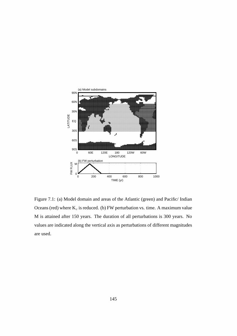
0 60E 120E 180 120W 60W 90S
60S
30S
EQ
30N
60N
90N
LONGITUDE
LAT
ITU
DE
(a) Model subdomains
0 200 400 600 800 10000
M
FW
FLU
X
TIME (yr)
(b) FW perturbation
Figure 7.1: (a) Model domain and areas of the Atlantic (green) and Pacific/ Indian
Oceans (red) where Kv is reduced. (b) FW perturbation vs. time. A maximum value
M is attained after 150 years. The duration of all perturbations is 300 years. No
values are indicated along the vertical axis as perturbations of different magnitudes
are used.
145

4
3
2
1D
EP
TH
(km
)
0
0
0
0
0
0
2018161412108642
−2
−2
−4 −4
1210
62
10
(a) NADW "on"
4
3
2
1
DE
PT
H (
km) 0
0 0 0 0
00
0
0−9−7 −6−5
−4 −3 −2−1−1
−2−3−4
−3−2−1
(b) NADW "off"
30S EQ 30N 60N
4
3
2
1
LATITUDE
DE
PT
H (
km)
0
0
0
0
0 0
0
0
0
−6−5 −4
−3 −2−1
−1−2
−3−4
−3−2
−1
1
(c) NADW "off" Kv reduced in Atl. by 2/3
Figure 7.2: Atlantic meridional overturning streamfunction (annual mean) for (a)
the steady NADW “on” state of the control experiment CNTRL, (b) the steady
NADW “off” state of CNTRL, and (c) the steady NADW “off” state when Kv is
reduced inside the Atlantic via multiplication by a factor of 2/3. Values are given in
Sv (1 Sv = 106 m3 sec−1).
146

0
5
10
15
20
25
30
Sv
(a) NADW formation
0 500 1000 1500 2000 2500 30000
2
4
6
8
10
TIME (year)
Sv
(b) AAIW reverse cell
1/4KV 1/3KV 1/2KV 2/3KV
Figure 7.3: Timeseries for experiments 1
4KVAtl (black) ,1
3KVAtl (blue), 1
2KVAtl
(red) and 2
3KVAtl (green) under a FW perturbation attaining a maximum value of
1.02 m/yr after 150 years. Timeseries are shown for (a) NADW production rate and
(b) the AAIW reverse cell. Values are given in Sv (1 Sv = 106 m3 sec−1).
147

0
5
10
15
20
25
30
Sv
(a) NADW formation
0 200 400 600 800 1000 1200 1400 1600 18000
5
10
15
TIME (year)
Sv
(b) AAIW reverse cell
1/3KVIP
−0.48 Sv
Figure 7.4: Timeseries for experiments 1
3KVPac under a FW perturbation attaining
a maximum of 1.7 m/yr after 150 years. Timeseries are shown for (a) NADW
production rate and (b) the AAIW reverse cell. Values are given in Sv (1 Sv = 106
m3 sec−1).
148

4
3
2
1
DE
PT
H (
km)
0
0
0
0
0
0
181614121086
42
−2 −2
1210 8 6
14
−4
(a) Kv reduced in Atlantic
30S EQ 30N 60N
4
3
2
1
LATITUDE
DE
PT
H (
km)
0
0
00
0
0
−1−2−3
−4 −3−2−1
−9 −8 −7−6 −5 −4−3−2
1−1 −2
(b) Kv reduced in Pacific
Figure 7.5: Atlantic meridional overturning streamfunction (annual mean) for (a)
experiment 1
3KVAtl, where Kv is reduced inside the Atlantic and (b) 1
3KVIP where
Kv is reduced inside the Pacific and Indian Ocean. Values are given in Sv (1 Sv =
106 m3 sec−1).
149

0
5
10
15
20
25
30
Sv
(a) NADW formation
0 500 1000 1500 2000 2500 30000
2
4
6
8
10
TIME (year)
Sv
(b) AAIW reverse cell
CNTRL 0.38 m/ yr 1/3KV
Atl 0.51 m/ yr
1/3KVAtl
1.02 m/ yr 1/3KV
Atl 1.53 m/ yr
Figure 7.6: Timeseries for experiment CNTRL under a perturbation attaining a
maximum value of 0.38 m/yr (blue) and experiment 1
3KVAtl under perturbations
attaining a maximum of 0.51 m/ yr (black), 1.02 m/ yr (green) and 2.04 m/ yr (red).
Timeseries are shown for (a) NADW production rate and (b) the AAIW reverse cell.
Values are given in Sv (1 Sv = 106 m3 sec−1).
150

Chapter 8
Concluding remarks
A variety of factors affecting global thermohaline circulation (THC) stability have
been investigated using a global intermediate complexity coupled model. We have
found a variety of implications for past climates and uncovered new uncertainties
in the THC response to high latitude freshening. Primitive equation ocean models
are a critically important tool in climate research. Although remote, one possi-
ble climatic response to global warming might be a collapse of North Antlantic
Deep Water (NADW) formation, resulting in a significant cooling of Northern Eu-
rope. Using a numerical climate model, we uncover new insight into the nature and
mechanisms behind a NADW collapse, as well as a hitherto unknown uncertainty
related to the use of such models for this purpose.
In particular, it remains unclear whether the degree of isopycnal diffusion simulated
in ocean models is realistic. Direct observations of this process are limited, as is
our knowledge of the appropriate coefficient to use for along-isopycnal diffusion
in ocean models. Based on this work, a modification of along-isopycnal mixing
schemes in ocean models may be required. Furthermore, we suggest possible focal
points for new research into the nature of the NADW “off” state in climate models.
In particular, the north-south branching of Antarctic Intermediate Water (AAIW)
151

north of Drake Passage is important for paleoclimatological studies of collapsed
NADW states that may have occurred in the past. Furthermore, we have introduced
a new angle in considering the role of vertical mixing and its spatial distribution in
maintaining stability of the collapsed NADW climate state that may provide fruitful
avenues of further enquiry.
152

Bibliography
Barker, J. B., P. F., 1977: The opening of Drake Passage. Marine Geology, 25,
15–34.
Bi, D., W. F. Budd, A. C. Hirst, and X. Wu, 2001: Collapse and reorganisation
of the Southern Ocean overturning under global warming in a coupled model.
Geophysical Research Letters, 28, 3927–3930.
— 2002: Response of the Antarctic circumpolar current transport to
global warming in a coupled model. Geophysical Research Letters, 29,
doi:10.1029/2002GL015919.
B oning, C. W., W. R. Holland, F. O. Bryan, G. Danabasoglu, and J. C. McWilliams,
1995: An overlooked problem in model simulations of thermohaline circulation
and heat transport in the Atlantic Ocean. Journal of Climate, 8, 515–523.
Broecker, W. S., 1991: The great ocean conveyor belt. Oceanography, 4, 79–87.
Bryan, F., 1986: High-latitude salinity effects and interhemispheric thermohaline
circulations. Nature, 323, 301–304.
— 1987: Parameter sensitivity of primitive equation ocean general circulation mod-
els. Journal of Physical Oceanography, 17, 970–985.
Bryan, F., S. Manabe, and M. J. Spelman, 1988: Interhemispheric asymmetry in
the transient response of a coupled ocean-atmosphere model to a CO2 forcing.
Journal of Physical Oceanography, 18, 851–867.
153

Bryan, K. and L. J. Lewis, 1979: A water mass model of the world ocean. Journal
of Geophysical Research, 84, 2503–2517.
Cox, M. D., 1987: Isopycnal diffusion in a z-coordinate ocean model. Ocean Mod-
elling, 74, 1–5.
— 1989: An idealized model of the world ocean. part I: The global-scale water
masses. Journal of Physical Oceanography, 19, 1730–1752.
Danabasoglu, G., J. C. McWilliams, and P. R. Gent, 1994: The role of mesoscale
tracer transports in the global ocean circulation. Science, 264, 1123–1126.
DeConto, R. M. and D. Pollard, 2004: Rapid Cenozoic glaciation of Antarctica
induced by declining atmospheric CO2. Nature, 421, 245–249.
Duffy, P. B. and K. Caldeira, 1997: Sensitivity of simulated salinity in a three
dimensional ocean model to upper-ocean transport of salt from sea-ice formation.
Geophysical Research Letters, 24, 1323–1326.
Duffy, P. B., K. Caldeira, J. Selvaggi, and M. I. Hoffert, 1997: Effects of subgrid-
scale mixing parametrisations on simulated distributions of natural 14c, tempera-
ture, and salinity in a three-dimensional ocean general circulation model. Journal
of Physical Oceanography, 27, 498–523.
Duffy, P. B., P. Eltgroth, A. J. Bourgois, and K. Caldeira, 1995: Effect of improved
subgrid scale transport of tracers on uptake of bomb radiocarbon in the GFDL
ocean general circulation model. Geophysical Research Letters, 22, 1065–1068.
England, M. H., 1992: On the formation of Antarctic Intermediate and Bottom
Water in ocean general circulation models. Journal of Physical Oceanography,
22, 918–926.
— 1995: Using chlorofluorcarbons to assess ocean climate models. Geophysical
Research Letters, 22, 3051–3054.
154

England, M. H., J. S. Godfrey, A. C. Hirst, and M. Tomczak, 1993: The mechanism
for Antarctic Intermediate Water renewal in a world ocean model. Journal of
Physical Oceanography, 23, 1553–1560.
England, M. H. and G. Holloway, 1998: Simulations of cfc content and water mass
age in the deep north atlantic. Journal of Geophysical Research, 103, 15885–
15901.
England, M. H. and S. Rahmstorf, 1999: Sensitivity of ventilation rates and ra-
diocarbon uptake to subgrid-scale mixing in ocean models. Journal of Physical
Oceanography, 29, 2802–2827.
Fanning, A. G. and A. J. Weaver, 1996: An atmospheric energy-moisture model:
climatology, interpentadal climate change and coupling to an ocean general cir-
culation model. Journal of Geophysical Research, 101, 15111–15128.
Gent, P. R. and J. C. McWilliams, 1990: Isopycnal mixing in ocean general circu-
lation models. Journal of Physical Oceanography, 20, 150–155.
Gerdes, R., 1993: A primitive equation ocean circulation model using a general ver-
tical coordinate transformation 2. Application to an overflow problem. Journal of
Geophysical Research, 98, 211–226.
Gill, A. E. and K. Bryan, 1971: Effects of geometry on the circulation of a three
dimensional hemisphere ocean model. Deep-Sea Research, 18, 685–721.
Gnanadesikan, A., 1999: A simple predictive model for the structure of the oceanic
pycnocline. Science, 283, 2077–2079.
Gnanadesikan, A. and R. W. Hallberg, 2000: On the relationship of the circumpolar
current to southern hemisphere winds in course-resolution ocean models. Journal
of Physical Oceanography, 30, 2013–2034.
Gordon, A. L., 1986: Interocean exchange of thermocline water. J. Geophys. Res.,
91, 5037–5046.
155

Gregory, J. M., O. A. Saenko, and A. J. Weaver, 2003: The role of the Atlantic
freshwater balance in the hyteresis of the meridional overturning circulation. Cli-
mate Dynamics, 21, 707–717, doi: 10.1007/s00382–003–0359–8.
Hasumi, H. and N. Suginohara, 1999: Effects of locally enhanced vertical diffusiv-
ity over rough bathymetry on the world ocean circulation. J. Geophys. Res., 104
(C10), 23367–23374.
Hirst, A. C. and W. Cai, 1994: Sensitivity of a world ocean GCM to changes in sub-
surface mixing parametrization. Journal of Physical Oceanography, 24, 1256–
1279.
Huber, M., L. Sloan, and C. Shellito, 2003: Early paleogene oceans and climate: A
fully coupled modeling approach using the NCAR CCSM. Geological Society of
America Special Paper 369, 0, 634.
Hughes, T. M. C. and A. J. Weaver, 1994: Multiple equilibria of an asymmetric
two-basin ocean model. Journal of Physical Oceanography, 24, 619–637.
Hunke, E. C. and J. K. Dukowicz, 1997: An elastic-viscous-plastic model for sea
ice dynamics. Journal of Physical Oceanography, 27, 1849–1867.
Kalnay, E., M. Kanamitsu, R. Kistler, W. Collins, D. Deaven, L. Gandin, M. Iredell,
S. Saha, G. White, J. Woollen, Y. Zhu, A. Leetmaa, and R. Reynolds., 1996: The
NCEP/NCAR 40-year re-analysis project. Bull. Amer. Meteor. Soc., 77, 437–471.
Kamenkovich, I. V. and E. S. Sarachik, 2004: Mecahnisms controlling the sensi-
tivity of the Atlantic Thermohaline Circulation to the parameterization of eddy
transports in ocean GCM. Journal of Physical Oceanography, 34, 1628–1647.
Kamenkovich, P. H. S., J. Marotzke, 2000: Factors affecting heat transport in an
ocean general circulation model. Journal of Physical Oceanography, 34, 175–
194.
156

Kennett, J. P., 1977: Cenozoic evolution of antarctic glaciation, the Circum Antarc-
tic Ocean, and their impact on global paleoceanography. Journal of Geophysical
Research, 82, 3843–3860.
Klinger, B. A. and S. Drijfhout, 2004: Remote wind-driven overturning in the ab-
sence of the Drake Passage effect. Journal of Physical Oceanography, 34, 1036–
1049.
Ledwell, J., E. Montgomery, K. Polzin, L. S. Laurent, R. Schmitt, and J. Toole,
2000: Evidence for enhanced mixing over rough topography in the abyssal ocean.
Nature, 403, 179–182.
Manabe, S. and R. J. Stouffer, 1988: Two stable equilibria of a coupled ocean-
atmosphere model. Journal of Climate, 1, 841–866.
— 1994: Multiple-century response of a coupled ocean-atmosphere model to an
increase of atmospheric carbon dioxide. Journal of Climate, 7, 5–23.
— 1999: Are two modes of thermohaline circulation stable? Tellus, 51A, 400–411.
McCartney, M. S., 1977: Subantarctic mode water. a voyage of discovery. M. V.
Angel, Ed., Pergamon Press, 0, 103–119.
Mikolajewicz, U., E. Maier-Reimer, T. J. Crowley, and K. Y. Kim, 1993: Effect of
Drake Passage and Panamanian gateways on the circulation of an ocean model.
Paleoceanography, 8, 409–426.
Mikolajewicz, U. and R. Voss, 2000: The role of the individual air-sea flux com-
ponents in co2-induced changes of the ocean’s circulation and climate. Climate
Dynamics, 16, 627–642.
Munk, W. H., 1966: Abyssal Recipes. Deep Sea Research, 13, 707–730.
Munk, W. H. and C. Wunsch, 1998: Abyssal Recipes II: Energetics of tidal and
wind mixing. Deep Sea Research, 45, 1977–2010.
157

Nong, G. T., R. G. Najjar, D. Seidov, and W. H. Peterson, 2000: Simulation of ocean
temperature change due to the opening of Drake Passage. Geophysical Research
Letters, 27, 2689–2692.
Pacanowski, R., 1995: MOM2 Documentation User’s Guide and Reference Man-
ual: GFDL Ocean Group Technical Report. NOAA, GFDL. Princeton, 232pp.
Prange, P., G. Lohmann, and A. Paul, 2003: Influence of vertical mixing on the ther-
mohaline hysteresis: Analysis of an OGCM. Journal of Physical Oceanography,
33, 1707–1719.
Rahmstorf, S., 1993: A fast and complete convection scheme for ocean models.
Ocean Modelling, 101, 9–11.
— 1995: Bifurcations of the Atlantic thermohaline circulation in response to
changes in the hydrological cycle. Nature, 378, 145–149.
— 1996: On the freshwater forcing and transport of the Atlantic thermohaline cir-
cultion. Climate Dynamics, 12, 799–811.
Rahmstorf, S. and M. H. England, 1997: On the influence of Southern Hemisphere
winds on North Atlantic deep water flow. Journal of Physical Oceanography, 25,
2040–2054.
Rahmstorf, S. and J. Willebrand, 1995: The role of temperature feedback in stabi-
lizing the thermohaline circulation. Journal of Physical Oceanography, 25, 787–
805.
Redi, M. H., 1982: Oceanic isopycnal mixing by coordinate rotation. Journal of
Physical Oceanography, 12, 1154–1158.
Rooth, C., 1982: Hydrology and ocean circulation. Prog. Oceanogr., 11, 131–149.
Saenko, O. A., J. M. Gregory, A. J. Weaver, and M. Eby, 2002: Distinguishing the
influences of heat, freshwater and momentum fluxes on ocean circulation and
climate. Journal of Physical Oceanography, 32, 3376–3395.
158

Saenko, O. A. and W. J. Merryfield, 2005: On the effect of topographically-
enhanced mixing on the global ocean circulation. Journal of Physical Oceanog-
raphy, 35, 826–834.
Saenko, O. A., A. J. Weaver, and J. M. Gregory, 2003: On the link between the two
modes of the ocean thermohaline circulation and the formation of global-scale
water masses. Journal of Climate, 16, 2797–2801.
Schmitt, R. W., P. S. Bogden, and C. E. Dorman, 1989: Evaporation minus precipi-
tation and density fluxes for the North Atlantic. Journal of Physical Oceanogra-
phy, 19, 1208–1221.
Schmittner, A. and A. J. Weaver, 2001: Dependence of multiple climate states on
ocean mixing parameters. Geophysical Research Letters, 28, 1027–1030.
Sijp, W. P. and M. H. England, 2004: Effect of the Drake Passage throughflow on
global climate. Journal of Physical Oceanography, 34, 1254–1266.
— 2005: On the role of the Drake Passage in controlling the stability of the ocean’s
thermohaline circulation. Journal of Climate, 18, 1957–1966.
Sørensen, J. V. T., J. Ribbe, and G. Shaffer, 2001: Sensitivity of a world ocean GCM
to changes in subsurface mixing parametrization. Journal of Physical Oceanog-
raphy, 31, 3295–3311.
Stommel, H., 1961: Thermohaline convection with two stable regimes of flow. Tel-
lus, 13, 224–230.
Stommel, H. and A. B. Arons, 1960: On the abyssal circulation of the world ocean,
I. an idealized model of the circulation pattern and amplitude in oceanic basins.
Deep-Sea Res., 6, 217–233.
Toggweiler, J. R. and H. Bjornsson, 2000: Drake passage and paleoclimate. Journal
of Quaternian Science, 15, 319–328.
159

Toggweiler, J. R. and B. L. Samuels, 1995: Effect of Drake Passage on the global
thermohaline circulation. Deep-Sea Research I, 42, 477–500.
Tsujino, H. and N. Suginohara, 1999: Thermohaline circulation enhanced by wind
forcing. Journal of Physical Oceanography, 29, 1506–1516.
Weaver, A. J., M. Eby, E. C. Wiebe, and co authors, 2001: The UVic Earth System
Climate Model: model description, climatology, and applications to past, present
and future climates. Atmosphere-Ocean, 39, 1067–1109.
Wu, X., F. Budd, V. I. Lytle, and R. A. Massom, 1999: The effect of snow on
Antarctic sea ice simulations in a coupled atmosphere-sea ice model. Climate
Dynamics, 15, 127–143.
Zang, S., R. J. Greatbatch, and C. A. Lin, 1993: A reexamination of the polar
halocline catastrophe and implications for coupled ocean-atmosphere modeling.
Journal of Physical Oceanography, 23, 287–299.
Zang, S., W. Schmitt, and R. X. Huang, 1999: The relative influence of diapycnal
mixing and hydrologic forcing on the stability of the thermohaline circulation.
Journal of Physical Oceanography, 29, 1096–1108.
160