cluster-weighted stochastic subgrid-scale modelling - · pdf filecluster-weighted stochastic...

Cluster-weighted stochastic subgrid-scale modelling

Frank Kwasniok

College of Engineering, Mathematics and Physical SciencesUniversity of Exeter

North Park Road, Exeter EX4 4QF, United [email protected]

ABSTRACT

This paper presents the main results of a recent publication(Kwasniok, 2011a).

A new approach for data-based stochastic parametrisation of unresolved scales and processes in numerical weatherand climate prediction models is introduced. The subgrid-scale model is conditional on the state of the resolvedscales, consisting of a collection of local models. A clustering algorithm in the space of the resolved variables iscombined with statistical modelling of the impact of the unresolved variables. The clusters and the parameters ofthe associated subgrid models are estimated simultaneously from data. The method is implemented and exploredin the framework of the Lorenz ’96 model using discrete Markov processes as local statistical models. Perfor-mance of the cluster-weighted Markov chain (CWMC) scheme isinvestigated for long-term simulations as wellas ensemble prediction. It clearly outperforms simple parametrisation schemes and compares favourably withanother recently proposed subgrid modelling scheme also based on conditional Markov chains.

1 Introduction

The dynamics of weather and climate encompass a wide range ofspatial and temporal scales. Due tothe nonlinear nature of the governing equations, which are the laws of fluid dynamics, thermodynamics,radiative energy transfer and chemistry, the different scales are dynamically coupled to each other. Finitecomputational resources limit the spatial resolution of weather and climate prediction models; small-scale processes such as convection, clouds or ocean eddies are not properly represented. The necessityarises to account for unresolved scales and processes through the use of some form of subgrid modelling.This is usually referred to as a closure in fluid dynamics and theoretical physics, and as a parametrisationin meteorology and climate science.

Traditionally, parametrisations of unresolved scales andprocesses in numerical weather and climateprediction models have been formulated deterministically. Such bulk formulae are expected to capturethe mean effect of small-scale processes in terms of some larger-scale resolved variables. However,there is in general a strong non-uniqueness of the unresolved scales with respect to the resolved scales.Thus, no one-to-one correspondence between values of the resolved variables and subgrid-scale effectscan be expected; rather, a particular realisation of the subgrid term can be imagined to be drawn from aprobability distribution conditional on the resolved variables.

Adding stochastic terms to climate models, in an attempt to capture the impacts of unresolved scales hasbeen suggested in a seminal paper by Hasselmann (1976). First implementations of this concept were inthe context of sea-surface temperature anomalies (Frankignoul and Hasselmann, 1977) and a conceptualzonally averaged climate model (Lemke, 1977). Another early study looked at regime behaviour in avery simple atmospheric model under stochastic forcing (Egger, 1981).

Despite impressive improvements in the forecast skill of numerical weather and climate prediction in the

ECMWF Workshop on Model Uncertainty, 20–24 June 2011 137

KWASNIOK, F.: CLUSTER-WEIGHTED STOCHASTIC SUBGRID-SCALE MODELLING

past decades, there are still limitations due to model uncertainty and error as well as problems in gen-erating initial conditions for ensembles. Forecast ensembles tend to be underdispersive (e. g., Buizza,1997), leading to overconfident uncertainty estimates and an underestimation of extreme weather events.Systematic biases are significant in subgrid-scale weatherphenomena and state-of-the-art ensemble pre-diction systems occasionally miss extreme weather events in the ensemble distribution. One way ofaddressing these issues relating to model imperfection is to deliberately introduce an element of un-certainty into the model. This can be done by randomisation of existing parametrisation schemes;approaches include multi-model, multi-parametrisation and multi-parameter ensembles (Palmer et al.,2005). A more systematic and comprehensive representationof model uncertainty may be achieved byintroducing stochastic terms into the equations of motion.This has been implemented in the form ofstochastically perturbed tendencies (Buizza et al., 1999)and, most recently, stochastic-dynamic subgridschemes (Palmer, 2001; Shutts, 2005; Berner et al., 2008). Ageneral feature of stochastic parametrisa-tions is that they enable the forecast ensemble to explore important regions of phase space better thanmore restricted deterministic parametrisations. See Palmer et al., 2005; Weisheimer et al., 2011 for anoverview and comparison of different methods for representing model uncertainty and error in weatherand climate prediction models.

There has been a lot of research activity on subgrid modelling in recent years in various contexts, fromtheoretical studies constructing deterministic equations for moments of coarse-grained variables usinga constrained measure of the system (Chorin et al., 1998), toa systematic stochastic mode reductionstrategy based on stochastic differential equations (Majda et al., 1999, 2003), to various approachesto stochastic convection parametrisation (Lin and Neelin,2000; Majda and Khouider, 2002; Plant andCraig, 2008). A particular class of subgrid models are schemes which are derived purely from data(Wilks, 2005; Crommelin and Vanden-Eijnden, 2008). While being less transparent from a physicspoint of view, they are potentially more accurate as they areless restricted by a priori assumptions.

The purpose of the present paper is twofold: Firstly, it generally proposes a new approach to data-basedstochastic subgrid parametrisation using the methodologyof cluster-weighted modelling. Secondly andmore specifically, a cluster-weighted Markov chain subgridscheme is outlined, building on recent workon conditional Markov chains (Crommelin and Vanden-Eijnden, 2008).

The paper is organised as follows: Section 2 introduces the general framework of cluster-weightedmodelling for subgrid parametrisation. In section 3, we describe the Lorenz ’96 system which is hereused as a testbed to explore the method. The detailed formulation of the subgrid parametrisation in thecontext of the Lorenz ’96 system and how to estimate its parameters from data is discussed in section4. Then the results are presented in section 5. The paper concludes with some general discussion andimplications.

2 Subgrid-scale parametrisation using cluster-weighted modelling

Assume the climate system is described by a high-dimensional state vectoru which is decomposed asu = (x,y) wherex is the part resolved in a given weather or climate predictionmodel of a particularspatial resolution and complexity, andy is the unresolved part. The true tendency ofx is schematicallygiven by

x = R(x)+ U(x,y) (1)

with R(x) being the resolved tendency, arising from the interactionsamong the resolved variablesx, andU(x,y) being the unresolved tendency, arising from interactions with the unresolved variablesy. In asimulation with the model resolving onlyx, we need to parametriseU(x,y). Such a parametrisation hasthe general form

U(x,y) ∼ f(x)+ η(x) (2)

138 ECMWF Workshop on Model Uncertainty, 20–24 June 2011


where f(x) is the deterministic part of the closure model andη(x) is a stochastic process generallydependent onx. A canonical choice for the deterministic part would be the conditional mean of theunresolved tendency:

f(x) = 〈U(x,y)|x〉 (3)

The stochastic componentη(x) is represented by a collection of local subgrid models, conditional onthe state of the resolved variables. We build on the approachof cluster-weighted modelling (Gershenfeldet al., 1999; Kwasniok, 2011b) which is suitably adapted here. A finite number of clusters is introducedin a space of clustering variablesz. The number of clusters isM andm is the cluster index, running from1 to M. The integer variablec takes values from 1 toM, according to which cluster has been chosen.Each cluster has an overall weightwm = p(c = m), satisfying the probabilistic constraintswm ≥ 0 and∑mwm = 1, as well as a clustering probability densityp(z|c = m), describing its domain of influencein the space of clustering variablesz. The vectorz is a suitably chosen (low-dimensional) subset orprojection ofx; it may also contain past values ofx, that is, a time-delay embedding (Sauer et al.,1991). Each cluster is associated with a local probabilistic subgrid modelp(η |v,c = m) which dependson a vector of variablesv. The vectorv might encompass present and past values of components orprojections ofx as well as past values ofη. The conditional probability density of the stochastic subgridtermη is expanded into a sum over the clusters:

p(η |z,v) =M

∑m=1

gm(z) p(η |v,c = m) (4)

The state-dependent weightsgm of the individual models are given by Bayes’ rule:

gm(z) = p(c = m|z) =wm p(z|c = m)

∑Mn=1wn p(z|c = n)

. (5)

The local model weights satisfygm ≥ 0 and∑mgm = 1. The cluster-weighted subgrid model has twotypes of conditioning on the resolved variables: the dependence of the model weightsgm on z and theexplicit dependence of the subgrid models onv. The vectorsz andv might overlap.

The clustering densitiesp(z|c = m) and the local subgrid modelsp(η |v,c = m) can take various forms.The canonical choice for the clustering densitiesp(z|c= m) in the continuous case is Gaussian. For non-negative or strongly skewed variables other choices may be more appropriate. One may also partitionthe space ofz into a finite number of bins; the clustering probabilities are then discrete probabilitydistributions over these bins. The subgrid modelsp(η |v,c = m) may be regression models onv withGaussian uncertainty. In the present study, they are actually Markov chains governing the switchingbetween discrete values ofη.

The parameters of the clusters and the subgrid models are estimated simultaneously from a learning dataset by maximising a suitably defined likelihood function. The number of clustersM is a hyperparameterof the method controlling the overall complexity of the subgrid model. It may be determined within thefitting procedure of the subgrid model by minimising the Akaike or Bayesian information criterion in thelearning data set, or by maximising the cross-validated likelihood function in a data set different fromthe learning data set. Alternatively, the number of clusters may be determined from the performance ofthe subgrid model in finite-time prediction or a long-term integration measured by a suitable metric ofinterest.

3 The Lorenz ’96 model

The Lorenz ’96 (L96) model (Lorenz, 1996) is used as a testbedto explore the new subgrid parametri-sation scheme. It has become popular in the weather and climate science community as a toy model



-6

-4

-2

0

2

-5 0 5 10

Bk

Xk

-4

-2

0

2

-5 0 5 10

Bk

- <

Bk|

Xk>

Xk

Figure 1: Left: Scatterplot of the subgrid term Bk versus the state Xk. The solid line indicates theconditional mean as estimated by a fifth-order polynomial least-squares fit. Right: Scatterplot of thedeviation from the conditional mean,Bk = Bk −〈Bk|Xk〉, versus the state Xk. The solid horizontallines indicate the valuesβil used in the CWMC subgrid scheme (see text).

of the atmosphere to test concepts and algorithms relating to predictability, model error, ensemblepost-processing and subgrid parametrisation (e. g., Lorenz, 1996; Palmer, 2001; Fatkullin and Vanden-Eijnden, 2004; Wilks, 2005; Crommelin and Vanden-Eijnden,2008). The model equations are

Xk = Xk−1(Xk+1−Xk−2)−Xk +F +Bk (6)

Yj,k =1ε

[

Yj+1,k(Yj−1,k−Yj+2,k)−Yj,k +hyXk]

(7)

with

Bk =hx

J ∑j

Yj,k (8)

andk = 1, . . . ,K; j = 1, . . . ,J. The variablesXk andYj,k are arranged on a circle. They can be interpretedeither as variables on a circle of constant latitude or as meridional averages, each representing a segmentof longitude. As such, the model is a spatially extended system. TheXk are large-scale, slow variables,each coupled to a collection of small-scale, fast variablesYj,k. The variables are subject to the periodicboundary conditionsXk = Xk+K , Yj,k = Yj,k+K andYj+J,k = Yj,k+1 reflecting the periodicity of the spatialdomain. The system is invariant under spatial translations; therefore all statistical properties are identicalfor all Xk. The model formulation employed here (Fatkullin and Vanden-Eijnden, 2004) is exactlyequivalent to the original formulation by Lorenz (1996). With X∗

k andY∗j,k denoting the variables in

the original system (Lorenz, 1996) with parametersF, h, c and b, the corresponding system in theformulation of eqs.(6)–(8) is obtained by a linear scaling of the variables (Xk = X∗

k andYj,k = bY∗j,k)

and the parameter settingε = 1c , hx = −hcJ

b2 andhy = h, leaving the forcingF unchanged. The presentformulation of the system makes the time scale separation between the slow and fast variables explicit inthe positive parameterε . If ε → 0, we have infinite time scale separation; ifε ≈ 1, there is no time scaleseparation. We here use the parameter settingK = 18, J = 20, F = 10, ε = 0.5, hx = −1 andhy = 1,which is the same as in Crommelin and Vanden-Eijnden (2008).The system has 18 large-scale and 360small-scale variables, 378 variables in total.

In a reduced model of the L96 system, only the variablesXk are resolved explicitly. The impact ofthe unresolved variablesYj,k on the resolved variablesXk is described by the termBk which is referredto as the subgrid term or unresolved tendency. It needs to be parametrised somehow in a reducedmodel in order to account for the impact of the unresolved variables. This constitutes the subgrid-scaleparametrisation problem in the context of the L96 model.

Figure 1 displays a scatterplot of the subgrid termBk versus the stateXk obtained from a long (post-transient) numerical integration of the L96 model. The meanof Bk conditional onXk as estimated



by a fifth-order polynomial least-squares fit is also indicated. A higher order of the polynomial doesnot improve the fit significantly. In practice, all numericalvalues of the conditional mean〈Bk|Xk〉 arecalculated using the fifth-order polynomial. There is a strong non-uniqueness of the subgrid term withrespect to the resolved state: For a fixed value ofXk, Bk can take on a range of values. The conditionalmean explains only 52.4% of the variance of the subgrid termBk. The properties of the conditionalprobability density functionp(Bk|Xk) depend strongly onXk. In particular, it is markedly non-Gaussianfor a range of values ofXk. Figure 1 also shows a scatterplot of the deviation of the subgrid term fromits conditional mean,Bk = Bk−〈Bk|Xk〉, versusXk.

4 Subgrid-scale modelling with cluster-weighted Markov chains

As an example for the methodology outlined in Section 2, a cluster-weighted subgrid scheme based onlocal Markov chains is developed and implemented for the L96model.

4.1 Model formulation

We here combine the framework of cluster-weighted modelling (Gershenfeld et al., 1999; Kwasniok,2011b) with the use of conditional Markov chains (Crommelinand Vanden-Eijnden, 2008) for stochas-tic subgrid-scale parametrisation. The subgrid termBk is replaced by a collection of discrete Markovprocesses conditional on the state of the resolved variables. The closure model is formulated indepen-dently for each resolved variableXk as there is only little spatial correlation in the subgrid term Bk inthe L96 system (Wilks, 2005). We choose to condition the subgrid model at timet both on the currentstateXk(t) and the incrementδXk(t) = Xk(t)−Xk(t −δ t) whereδ t is the sampling interval of the data.This choice is motivated by the fact that the probability density function of the subgrid termBk has beenshown to depend also on the incrementδXk (Crommelin and Vanden-Eijnden, 2008). It seems conceiv-able that the probability density of the subgrid term could be further sharpened by conditioning on morepast values ofXk but we restrict ourselves to just one past value for simplicity.

The subgrid model is derived from an equally sampled data setof lengthN, {Xαk ,δXα

k , Bαk }

Nα=1. Here

and in the following, a subscript or superscriptα refers to time in an equally sampled time series withsampling intervalδ t and runs from 1 toN. A data point(Xk,δXk, Bk) is mapped to a discrete state(s,d,b)by partitioning the(Xk,δXk, Bk)-space into bins. TheXk-space is divided intoNX disjoint intervals

{I Xi }NX

i=1; we haves= i if Xk ∈ I Xi . TheδXk-space is divided intoNδX disjoint intervals{I δX

j }NδX

j=1;

we haved = j if δXk ∈ I δXj . Givens= i, the range of possible values ofBk is divided intoNB disjoint,

equally populated intervals{I Bil }

NB

l=1; we haveb= l if Bk ∈I Bil . The subgrid termBk is then represented

by a set ofNB discrete values{βil }NBl=1 given by the mean ofBk in each interval:

βil =∑α Bα

k 1(sα = i)1(bα = l)

∑α 1(sα = i)1(bα = l)(9)

We introduceM clusters in the discrete(s,d,b)-space. Each cluster has an overall weight or probabilityof that cluster being chosen,wm = p(c = m), and a clustering probability distributionψmi j = p(s =i,d = j|c = m), describing its domain of influence in(s,d)-space. The parameters of the clusters sat-isfy a couple of probabilistic constraints. The overall weights form a probability distribution:wm ≥ 0,∑mwm = 1. The clustering probability distributions satisfyψmi j ≥ 0 and∑i, j ψmi j = 1. The clustersare required to add up to the joint climatological distribution (invariant measure) ofs andd, that is,∑mwmψmi j = p(s= i,d = j) = ρi j whereρi j is empirically given as the fraction of data points in thesebins: ρi j = 1

N ∑α 1(sα = i)1(dα = j). It follows that the clusters also sum up to the marginal climato-logical distributions:∑m, j wmψmi j = p(s= i) = ∑ j ρi j as well as∑m,i wmψmi j = p(d = j) = ∑i ρi j .



Each cluster is associated with a Markov chain in the discrete spaceb described by an(NB×NB) tran-sition matrixAm with componentsAml1l2 = p(bα = l2|bα−1 = l1,cα = m). The matricesAm are row-stochastic matrices, that is,Aml1l2 ≥ 0 and∑l2 Aml1l2 = 1.

The conditional probability distribution forbα is modelled as a sum over the clusters:

p(bα |bα−1,sα ,dα) =M

∑m=1

gm(sα ,dα)Ambα−1bα . (10)

The state-dependent model weights are given by Bayes’ rule as

gm(i, j) = p(c = m|s= i,d = j) =wmψmi j

∑Mn=1wnψni j

=wmψmi j

ρi j. (11)

The Markov chain is effectively governed by local transition matricesAloc(i, j) = ∑mgm(i, j)Am whichas a convex combination of row-stochastic matrices are always row-stochastic matrices. The subgridmodel jumps according to the local Markov process between the NB possible values{βil }NB

l=1 given byeq.(9) fors= i. The mean local model weights are found to be〈gm〉 = 1

N ∑α gm(sα ,dα) = wm. Hencethe overall weightwm can be interpreted as the fraction of the data set (or the invariant measure of thesystem) accounted for by the clusterm.

The number of clustersM, the numbers of binsNX andNδX as well as the number of statesNB of theMarkov chain are hyperparameters of the method which have tobe fixed beforehand; they control theoverall complexity of the closure model. We call this subgrid model a cluster-weighted Markov chain(CWMC) model.

Given an equally sampled learning data set of lengthN, {b0,s1,d1,b1, . . . ,sN,dN,bN}, the parametersof the CWMC subgrid model are estimated according to the maximum likelihood principle using theexpectation-maximisation (EM) algorithm (Dempster et al., 1977; Kwasniok, 2011a, 2011b).

4.2 Model integration

The time integration of the reduced model with the CWMC subgrid scheme proceeds as follows: Thesubgrid scheme is constructed at time stepδ t; the deterministic equations for the resolved variables areintegrated with time steph determined by the employed numerical scheme, stability andthe desiredaccuracy. These two time steps may be different; typically,δ t is larger thanh. Assume for simplicitythat δ t is an integer multiple ofh: δ t = Nsteph. We then use a split-integration scheme (Crommelinand Vanden-Eijnden, 2008). The resolved dynamics are integrated with time steph; the subgrid modelis propagated with time stepδ t, updated only everyNstep time steps. At timetα−1, let the systemstate beXα−1

k falling in bin sα−1 and let the state of the Markov chain of the subgrid model bebα−1.The stateXα

k at time tα is calculated by propagating the resolved variablesNstep times with step sizeh using the derivative given by eq.(6) withBk set to〈Bk|Xα−1

k 〉+ βsα−1bα−1. If Xαk falls in bin sα and

δXαk = Xα

k −Xα−1k falls in bin dα the next state of the Markov chainbα is determined by randomly

drawing from the probability distribution given by eqs.(10) and (11). Then the subgrid termBk is set to〈Bk|Xα

k 〉+ βsα bα for the next integration cycle. One could also choose to update the deterministic partof the closure model at time steph. In the present model setting there is virtually no difference betweenthese two possibilities provided the sampling intervalδ t is not too large as the dependence of〈Bk|Xk〉on Xk is quite smooth. The rarer update is computationally more efficient.

5 Results

The full L96 model is integrated for 1000 time units of post-transient dynamics using the Runge-Kuttascheme of fourth order with step size 0.002. The state vectoris archived at a sampling intervalδ t = 0.01,



resulting in a data set containing 100000 data points. The CWMC closure scheme is constructed fromthis data set. Such a large learning data set, virtually corresponding to the limit of infinite data, is usedhere to get rid of any sampling issues for the parameter estimates and study the ideal behaviour of themethod. It should be noted that a very similar performance ofthe reduced model to that presented herecan already be obtained with a much shorter learning data set(∼ 5000 data points). We useNX = 4 in-tervals inXk-space. They are located between -5.5 and 10.5 and have equalsize. We then extend the firstand the last interval to minus and plus infinity, respectively. Thus, the intervals areI X

1 = (−∞,−1.5],I X

2 = (−1.5,2.5], I X3 = (2.5,6.5] andI X

4 = (6.5,∞). In δX-space we useNδX = 2 intervals givenasI δX

1 = (−∞,0] andI δX2 = (0,∞), corresponding to downwards and upwards direction of the tra-

jectory. The number of bins for the subgrid term, that is, thenumber of states of the Markov chain isset toNB = 3. The valuesβil used in the CWMC scheme given by eq.(9) are displayed in Fig. 1. Theresolution of the binnings was determined from the performance of the resulting reduced model. Westudied larger values for all of the parametersNX, NδX andNB but a higher resolution in the binning ofany of the variables does not visibly improve the model. CWMCclosure schemes were estimated fromthe data set with increasing number of clusters, starting from M = 1. Based on the performance of thereduced model,M = 2 is found to be the optimal number of clusters. There is no significant furtherimprovement when using more than 2 clusters.

The CWMC scheme is compared to two simple generic parametrisation schemes: a deterministic clo-sure scheme and the AR(1) scheme proposed by Wilks (2005). The deterministic scheme consists inparametrisingBk by the conditional mean as estimated by the fifth-order polynomial fit shown in Fig. 1:Bk ∼ 〈Bk|Xk〉. The AR(1) scheme modelsBk by the conditional mean plus an AR(1) process:

Bαk = Bα

k −〈Bk|Xαk 〉 = φ Bα−1

k + σξ (12)

ξ denotes Gaussian white noise with zero mean and unit variance, σ is the standard deviation of thedriving noise. ForBk, this amounts to an AR(1) process with state-dependent mean〈Bk|Xk〉 but constantautoregressive parameter and standard deviation of the noise. A least-squares fit to the time series ofBk

at time stepδ t = 0.01 yieldsφ = 0.9977 (corresponding to ane-folding time of 4.25 time units) andσ =0.059. The standard deviation of the AR(1) process isσ√

1−φ2= 0.866, equal to the standard deviation

of Bk. The reduced models with the deterministic and the AR(1) subgrid schemes are integrated in timein a manner analogous to that described in subsection 4.2 forthe CWMC scheme, updating the subgridterm at time stepδ t.

The CWMC scheme is also compared to the subgrid modelling study by Crommelin and Vanden-Eijnden(2008) based on conditional Markov chains using the L96 system with exactly the same parametersetting as an example. They condition the Markov chain onXα

k andXα−1k , both partitioned into 16 bins.

Taking into account that due to the autocorrelation of the system at lagδ t only transitions within thesame bin and into neighbouring bins actually occur this roughly (not exactly) corresponds toNX = 16andNδX = 3 in the present setting. Then a separate transition matrix (with NB = 4) is determined foreach pair of bins, amounting to about 45 active transition matrices. We occasionally refer to this subgridmodel for comparison as the full Markov chain scheme. The present CWMC scheme offers a muchmore condensed description of the subgrid term. It uses onlyM = 2 independent transition matrices.Moreover, a much coarser binning (NX = 4, NδX = 2) and onlyNB = 3 states in the Markov chain areused. The number of parameters to be estimated from data is actually about 40 times larger in the fullMarkov chain scheme than in the CWMC scheme. Consequently, alonger learning data set is necessaryto estimate the full Markov chain model.

5.1 Long-term dynamics of the reduced model

We investigate to what extent the reduced models with the various subgrid schemes are able to reproducethe statistical properties of the long-term behaviour of the large-scale variablesXk in the full L96 model.



Mean Std. dev. D

Full L96 model 2.39 3.52Deterministic scheme 2.53 3.56 0.017AR(1) scheme 2.51 3.57 0.015CWMC scheme 2.40 3.51 0.004

Table 1: Mean and standard deviation of Xk in the L96 model and the reduced models with thevarious subgrid schemes. The last column gives the Kolmogorov-Smirnov distance between theprobability distribution of Xk in the reduced model and that in the full L96 model.

0

0.05

0.1

-10 -5 0 5 10 15

prob

abili

ty d

ensi

ty

Xk

Figure 2: Probability density function of Xk in the full L96 model (solid) and in reduced models withdeterministic subgrid scheme (dot-dashed), AR(1) scheme (dotted) and CWMC scheme (dashed).

The reduced models are integrated in time as described in subsection 4.2 using a fourth-order Runge-Kutta scheme with step sizeh= 0.002. The closure model is updated every fifth time step. The reducedmodel with CWMC subgrid scheme runs more than 30 times fasterthan the full L96 model. Startingfrom random initial conditions, after discarding the first 50 time units of the integration to eliminatetransient behaviour 2500 time units worth of data are archived at a sampling interval ofδ t = 0.01,resulting in time series of length 250000. All the results reported below are calculated from these timeseries.

Figure 2 shows the probability density function ofXk in the reduced models with the three differentclosure schemes and that of the full L96 model for comparison. Additionally, table 1 gives the meanand the standard deviation of the PDFs. It also lists the deviation of the probability distributions ofthe reduced models from that of the full L96 model as measuredby the Kolmogorov-Smirnov statisticD = maxXk|Φ(Xk)−Φr(Xk)| whereΦ is the (cumulative) probability distribution of the L96 model andΦr is the probability distribution of the reduced model. All models reproduce the PDF quite well.The deterministic and the AR(1) schemes are very close to each other. The CWMC scheme offers animprovement on the two other schemes; it is about as good as the full Markov chain scheme (Crommelinand Vanden-Eijnden, 2008). The deterministic and the AR(1)schemes exhibit a considerable shift inthe mean state and slightly too much variance. The CWMC scheme has almost exactly the correct meanand variance.

In order to monitor the spatial pattern of variability in thesystem, the Fourier wave spectrum of thesystem is displayed in Figure 3. At each instant in time, the discrete spatial Fourier transform of thestate vectorX = (X1, . . . ,XK) is calculated, giving the (complex) wave vectorG = (G0, . . . ,GK−1) withGν = G∗

K−ν for ν = 1, . . . ,K − 1. The wave variance of wavenumberν is then 〈|Gν −〈Gν〉|2〉 forν = 0, . . . ,K−1 where〈·〉 denotes the time average. Figure 3 also shows the correlation of two variablesXk andXk+l , separated by a lagl on the circle. The deterministic and the AR(1) closure schemes give



0

0.5

1

1.5

2

0 1 2 3 4 5 6 7 8 9

wav

e va

rianc

e

wavenumber

-0.5

0

0.5

1

0 1 2 3 4 5 6 7 8 9

corr

elat

ion

spatial lag l

Figure 3: Left: Wave variances in the full L96 model (solid) and in reduced models with deter-ministic subgrid scheme (dot-dashed), AR(1) scheme (dotted) and CWMC scheme (dashed). Right:Correlation of Xk and Xk+l in the full L96 model (solid) and in reduced models with deterministicsubgrid scheme (dot-dashed), AR(1) scheme (dotted) and CWMC scheme (dashed).

-0.4

-0.2

0

0.2

0.4

0.6

0.8

1

0 1 2 3 4 5 6 7 8 9 10

auto

corr

elat

ion

time lag

-0.4

-0.2

0

0.2

0.4

0.6

0 1 2 3 4 5 6 7 8 9 10

cros

s-co

rrel

atio

n

time lag

Figure 4: Left: Autocorrelation function of Xk in the full L96 model (solid) and in reduced mod-els with deterministic subgrid scheme (dot-dashed), AR(1)scheme (dotted) and CWMC scheme(dashed). Right: Cross-correlation function of Xk and Xk+1 in the full L96 model (solid) and inreduced models with deterministic subgrid scheme (dot-dashed), AR(1) scheme (dotted) and CWMCscheme (dashed).

very similar results. They exhibit large error; the peak in the wave spectrum is too small and broad,spread out over wavenumbers 3 and 4. The CWMC scheme capturesthe sharp peak at wavenumber 3correctly and reproduces the whole spectrum almost perfectly; it performs as well as the full Markovchain model (Crommelin and Vanden-Eijnden, 2008). The sameeffect manifests itself in the spatialcorrelations. With the deterministic and the AR(1) schemes, the maximum positive correlation at lag 6(associated with wavenumber 3) is shifted to lags 4 and 5 due to too much variance in the shorter waveswith wavenumbers 4 and 5. The CWMC scheme reproduces the spatial correlations almost perfectly.

We now look at the behaviour of the models in the time domain. Figure 4 gives the autocorrelationfunction of Xk and the cross-correlation function of neighbouring variables Xk and Xk+1. They bothhave oscillatory behaviour over long time scales. The deterministic and the AR(1) scheme have theamplitude of the oscillations too small and there is a phase shift compared to the full L96 model. TheCWMC scheme performs much better; the amplitude of the oscillations is correct and there is only asmall phase shift visible at large time lags. The full Markovchain model is slightly better than theCWMC scheme; it reproduces the auto- and cross-correlationfunctions almost perfectly (Crommelinand Vanden-Eijnden, 2008).



0

0.05

0.1

0.15

0.2re

lativ

e fr

eque

ncy

rank

0

0.05

0.1

0.15

0.2

rela

tive

freq

uenc

y

rank

0

0.05

0.1

0.15

0.2

rela

tive

freq

uenc

y

rank

Figure 5: Rank histograms for ensembles with the deterministic subgrid scheme (top left), the AR(1)scheme (top right) and the CWMC scheme (bottom). Predictionlead time isτ = 2; ensemble size isNens= 20. The dashed horizontal lines indicate the expected relative frequency under rank unifor-mity.

5.2 Ensemble prediction

We investigate the predictive skill of the reduced models with the different parametrisations. Given thestochastic nature of the models an ensemble prediction framework appears to be most appropriate. Weconstruct ensembles which account for both model and initial condition uncertainty. In these ensembles,each ensemble member starts from a randomly perturbed initial condition. We follow the procedure inCrommelin and Vanden-Eijnden (2008). The perturbations are drawn from a Gaussian distribution withzero mean and a standard deviation of 0.15 (about 4% of the climatological standard deviation ofXk),independently for each componentXk. The predictive skill turns out to be rather insensitive to the exactvalue of the amplitude of the perturbations. This simple generation of ensembles appears to be sufficienthere for the purpose of comparing different subgrid-scale models. We do not sample unstable directionsin phase space more heavily (as is done by Wilks (2005)) or identify fastest-growing perturbations usingsingular vectors. 10000 initial conditions are used taken from a long integration of the full L96 model,separated by 5 time units.

In order to assess the ensemble spread we use rank histograms(Hamill, 2001). Rank histograms givethe relative frequency of the rank of the true state in theNens+ 1 member distribution formed by theensemble members and the true state. Ideally, the rank histogram should be flat corresponding to auniform distribution of the rank of the true state. For underdispersed ensembles the true state occupiesthe extreme ranks too often, showing up in a U-shaped rank histogram. Conversely, for overdispersedensembles the extreme ranks are occupied too rarely, givingan inverse U-shape in the rank histogram.Figure 5 shows rank histograms for the different parametrisation schemes. The ensemble size isNens=20; the prediction lead time isτ = 2. The rank histograms are representative also for other lead times.With the deterministic closure scheme the ensembles are strongly underdispersed. For the AR(1) scheme



0

0.2

0.4

0.6

0.8

1

0 1 2 3 4 5

anom

aly

corr

elat

ion

lead time

0

5

10

15

20

0 1 2 3 4 5

root

mea

n sq

uare

err

or

lead time

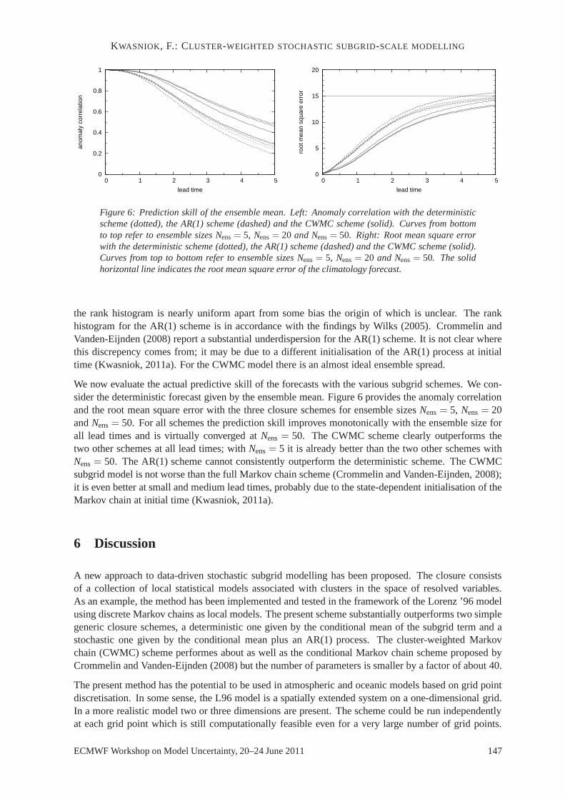
Figure 6: Prediction skill of the ensemble mean. Left: Anomaly correlation with the deterministicscheme (dotted), the AR(1) scheme (dashed) and the CWMC scheme (solid). Curves from bottomto top refer to ensemble sizes Nens= 5, Nens= 20 and Nens= 50. Right: Root mean square errorwith the deterministic scheme (dotted), the AR(1) scheme (dashed) and the CWMC scheme (solid).Curves from top to bottom refer to ensemble sizes Nens= 5, Nens= 20 and Nens= 50. The solidhorizontal line indicates the root mean square error of the climatology forecast.

the rank histogram is nearly uniform apart from some bias theorigin of which is unclear. The rankhistogram for the AR(1) scheme is in accordance with the findings by Wilks (2005). Crommelin andVanden-Eijnden (2008) report a substantial underdispersion for the AR(1) scheme. It is not clear wherethis discrepency comes from; it may be due to a different initialisation of the AR(1) process at initialtime (Kwasniok, 2011a). For the CWMC model there is an almostideal ensemble spread.

We now evaluate the actual predictive skill of the forecastswith the various subgrid schemes. We con-sider the deterministic forecast given by the ensemble mean. Figure 6 provides the anomaly correlationand the root mean square error with the three closure schemesfor ensemble sizesNens= 5, Nens= 20andNens= 50. For all schemes the prediction skill improves monotonically with the ensemble size forall lead times and is virtually converged atNens= 50. The CWMC scheme clearly outperforms thetwo other schemes at all lead times; withNens= 5 it is already better than the two other schemes withNens= 50. The AR(1) scheme cannot consistently outperform the deterministic scheme. The CWMCsubgrid model is not worse than the full Markov chain scheme (Crommelin and Vanden-Eijnden, 2008);it is even better at small and medium lead times, probably dueto the state-dependent initialisation of theMarkov chain at initial time (Kwasniok, 2011a).

6 Discussion

A new approach to data-driven stochastic subgrid modellinghas been proposed. The closure consistsof a collection of local statistical models associated withclusters in the space of resolved variables.As an example, the method has been implemented and tested in the framework of the Lorenz ’96 modelusing discrete Markov chains as local models. The present scheme substantially outperforms two simplegeneric closure schemes, a deterministic one given by the conditional mean of the subgrid term and astochastic one given by the conditional mean plus an AR(1) process. The cluster-weighted Markovchain (CWMC) scheme performes about as well as the conditional Markov chain scheme proposed byCrommelin and Vanden-Eijnden (2008) but the number of parameters is smaller by a factor of about 40.

The present method has the potential to be used in atmospheric and oceanic models based on grid pointdiscretisation. In some sense, the L96 model is a spatially extended system on a one-dimensional grid.In a more realistic model two or three dimensions are present. The scheme could be run independentlyat each grid point which is still computationally feasible even for a very large number of grid points.



In a more realistic model setting the vector of variablesz one would like to condition the model on islikely to be of higher dimension than in the L96 model. A conditioning based on binning into disjointintervals as in Crommelin and Vanden-Eijnden (2008) then becomes rapidly impractical and some formof clustering may be crucial to construct any feasible subgrid scheme.

The method of cluster-weighted subgrid modelling is more general than just a refinement or improve-ment of the conditional Markov chain scheme of Crommelin andVanden-Eijnden (2008). Differentclustering algorithms can be combined with various local statistical models. The method has also beenused to construct a closure for a low-order model of atmospheric low-frequency variability based onempirical orthogonal functions (EOFs) (Kwasniok, 2011c).

The present approach is purely data-driven and not based on physical considerations. This may bea strength as well as a weakness. Empirical schemes are potentially more accurate as they are freefrom constraining a priori assumptions. On the other hand, data-based models are sometimes criticisedas not helping with our understanding of the physics of the system. This drawback is here mitigatedby the transparent architecture of cluster-weighted modelling. The local models have meaningful andinterpretable parameters. Indeed, the clusters here represent phases of an oscillation in(Xk, Bk)-space(Kwasniok, 2011a). This gives some hope that clusters couldpotentially be linked to physical processeswhen the technique was applied to a more realistic system.

There might be potential for improvement in combining predictive, purely data-driven subgrid schemeslike the present approach with parametrisation schemes based more on physical reasoning or stochasticdynamical systems theory. Approaches like Majda et al. (1999, 2003) are able to derive the structuralform of the closure model for a given system. This information might be used to guide the choice ofstatistical model or place a priori constraints on the parameters.

References

Berner, J., F. J. Doblas-Reyes, T. N. Palmer, G. Shutts, and A. Weisheimer (2008). Impact of a quasi-stochastic cellular automaton backscatter scheme on the systematic error and seasonal predictionskill of a global climate model.Phil. Trans. R. Soc. A, 366, 2559–2577.

Buizza, R. (1997). Potential forecast skill of ensemble prediction, and spread and skill distributions ofthe ECMWF ensemble prediction system.Mon. Wea. Rev., 125, 99–119.

Buizza, R., M. J. Miller, and T. N. Palmer (1999). Stochasticsimulation of model uncertainties in theECMWF ensemble prediction system.Q. J. R. Meteorol. Soc., 125, 2887–2908.

Chorin, A. J., A. P. Kast, and R. Kupferman (1998). Optimal prediction of underresolved dynamics.Proc. Natl. Acad. Sci. USA, 95, 4094–4098.

Crommelin, D. and E. Vanden-Eijnden (2008). Subgrid-scaleparameterization with conditional Mar-kov chains.J. Atmos. Sci., 65, 2661–2675.

Dempster, A. P., N. M. Laird, and D. B. Rubin (1977). Maximum likelihood from incomplete data viaEM algorithm.J. Roy. Stat. Soc. B, 39, 1–38.

Egger, J. (1981). Stochastically driven large-scale circulations with multiple equilibria.J. Atmos. Sci.,38, 2606–2618.

Fatkullin, I. and E. Vanden-Eijnden (2004). A computational strategy for multiscale systems withapplications to Lorenz 96 model.J. Comput. Phys., 200, 605–638.

Frankignoul, C. and K. Hasselmann (1977). Stochastic climate models. Part II. Application to sea-surface temperature anomalies and thermocline variability. Tellus, 29, 289–305.



Gershenfeld, N., B. Schoner, and E. Metois (1999). Cluster-weighted modelling for time series analy-sis.Nature, 397, 329–332.

Hamill, T. M. (2001). Interpretation of rank histograms forverifying ensemble forecasts.Mon. Wea.Rev., 129, 550–560.

Hasselmann, K. (1976). Stochastic climate models. Part I. Theory.Tellus, 28, 473–485.

Kwasniok, F. (2011a). Data-based stochastic subgrid-scale parametrisation: an approach using cluster-weighted modelling.Phil. Trans. R. Soc. A, in press.

Kwasniok, F. (2011b). Cluster-weighted time series modelling based on minimising predictive igno-rance, submitted.

Kwasniok, F. (2011c). Nonlinear stochastic low-order modelling of atmospheric low-frequency vari-ability using a regime-dependent closure scheme, submitted.

Lemke, P. (1977). Stochastic climate models. Part III. Application to zonally averaged energy models.Tellus, 29, 385–392.

Lin, J. W.-B. and J. D. Neelin (2000). Influence of a stochastic moist convective parametrization ontropical climate variability.Geophys. Res. Lett., 27, 3691–3694.

Lorenz, E. N. (1996). Predictability – a problem partly solved. InProc. ECMWF Seminar on Pre-dictability, vol. 1, pp. 1–18, Reading, UK, ECMWF.

Majda, A. J. and B. Khouider (2002). Stochastic and mesoscopic models for tropical convection.Proc.Natl. Acad. Sci. USA, 99, 1123–1128.

Majda, A. J., I. Timofeyev, and E. Vanden-Eijnden (1999). Models for stochastic climate prediction.Proc. Natl. Acad. Sci. USA, 96, 14687–14691.

Majda, A. J., I. Timofeyev, and E. Vanden-Eijnden (2003). Systematic strategies for stochastic modereduction in climate.J. Atmos. Sci., 60, 1705–1722.

Palmer, T. N. (2001). A nonlinear dynamical perspective on model error: a proposal for non-localstochastic-dynamic parameterization in weather and climate prediction models.Q. J. Roy. Me-teor. Soc., 127, 279–304.

Palmer, T. N., G. J. Shutts, R. Hagedorn, F. J. Doblas-Reyes,T. Jung, and M. Leutbecher (2005).Representing model uncertainty in weather and climate prediction. Annu. Rev. Earth Planet. Sci.,33, 163–193.

Plant, R. S. and G. C. Craig (2008). A stochastic parameterization for deep convection based onequilibrium statistics.J. Atmos. Sci., 65, 87–105.

Sauer, T., J. A. Yorke, and M. Casdagli (1991). Embedology.J. Stat. Phys., 65, 579.

Shutts, G. (2005). A kinetic energy backscatter algorithm for use in ensemble prediction systems.Q. J. Roy. Meteor. Soc., 131, 3079–3102.

Weisheimer, A., T. N. Palmer, and F. J. Doblas-Reyes (2011).Assessment of representations of modeluncertainty in monthly and seasonal forecast ensembles.Geophys. Res. Lett., 38, L16703.

Wilks, D. S. (2005). Effects of stochastic parametrizations in the Lorenz ’96 system.Q. J. Roy. Me-teor. Soc., 131, 389–407.


150 ECMWF Workshop on Model Uncertainty, 20 – 24 June 2011

cluster-weighted stochastic subgrid-scale modelling - · pdf filecluster-weighted stochastic...

Documents