the effect of real estate prices on banks’ lending channel
TRANSCRIPT
The Effect of Real Estate Prices on Banks’ Lending Channel
Makoto Hazama Kaoru Hosono
and Iichiro Uesugi
March, 2016
Grant-in-Aid for Scientific Research(S) Real Estate Markets, Financial Crisis, and Economic Growth
: An Integrated Economic Approach
Working Paper Series No.53
HIT-REFINED PROJECT Institute of Economic Research, Hitotsubashi University
Naka 2-1, Kunitachi-city, Tokyo 186-8603, JAPAN Tel: +81-42-580-9145
E-mail: [email protected] http://www.ier.hit-u.ac.jp/hit-refined/
The Effect of Real Estate Prices on Banks’ Lending Channel*
Makoto Hazama† Kaoru Hosono‡ Iichiro Uesugi§
March 13, 2016
Abstract The shocks to real estate prices potentially have effects on banks’ balance sheets, their lending behavior, and eventually economic activities. We examine the existence of the bank lending channel in Japan during the 2007–2013 global financial crisis. We identify the heterogeneous shocks to real estate prices that affect banks by summarizing the land prices of their borrowing firms. We use a comprehensive database on firm-bank relationships as well as information on land prices for more than 20,000 locational points in Japan. We find that after controlling for fixed effects, a bank that faces a rise in land prices increases its capital, total loans, real estate loans, and loans backed by real estate collateral. We also find that the increased land prices do not significantly change the amount of non-real estate loans or loans without real estate collateral. Further, after controlling for time-varying firm fixed effects, increased land prices cause banks to reduce their transactional relationships with firms both in terms of extensive and intensive margins. We provide several possible explanations for the difference in the results between bank-level estimations and matched bank-firm estimations. Key Words: Bank Lending Channel, Real Estate Prices, Portfolio Reallocation. JEL Classification Numbers: E44, E51, G21.
* This study is conducted as a part of the Project on Corporate Finance and Firm Dynamics undertaken at the Research Institute of Economy, Trade and Industry (RIETI) and the Hitotsubashi Project on Real Estate, Financial Crisis, and Economic Dynamics (HIT-REFINED). We are grateful for fruitful discussion with Takashi Hanagaki. We also thank Michio Suzuki, Arito Ono, Masahiko Shibamoto, Chihiro Shimizu, Peng Xu, and participants at the JEA Meeting (2015 Autumn), 9th Regional Banking Conference, and the Hitotsubashi-RIETI International Workshop for valuable comments. I. Uesugi gratefully acknowledges financial support from the Grant-in-Aid for Scientific Research (S) No. 25220502, JSPS. † Graduate School of Economics, Hitotsubashi University. ‡ Gakushuin University. § Correspondence author. Institute of Economic Research, Hitotsubashi University, and RIETI. Email: [email protected]
1
1. Introduction
Massive fluctuations in real estate prices have frequently created booms (or sometimes
bubbles) and have triggered a number of financial crises. Some of the recent crises are the US
subprime mortgage and subsequent global financial crisis that started in 2007, the Japanese
banking crisis in the 1990s, and the Norwegian and Swedish banking crises in the early 1990s.
The research observes a link between the downturns in real estate prices and financial crises not
only in developed but also in developing economies. Analyzing the banking crises that occurred
in emerging markets in the past 30 years, Reinhart and Rogoff (2009, pp. 280) find that the most
important predictor of a crisis is the change in housing prices. If not triggering financial crises,
even moderate fluctuations in real estate prices affect real economic activities. Crowe et al.
(2011), for example, report that recessions subsequent to the burst of real estate booms are
longer and deeper than recessions without such booms.
Real estate prices are likely to affect the real economy through the availability and cost of
credit. Bernanke and Gertler (1989) and Kiyotaki and Moore (1997), among others, formalize
such a financial link in their general equilibrium models by focusing on a borrower’s net worth
(Bernanke and Gertler) or the value of collateral that a borrower pledges to obtain credit
(Kiyotaki and Moore). These two studies show that shocks to net worth or the value of collateral
affect capital investment, which amplifies the initial shocks. In tandem with the borrowers’ net
worth and collateral values, real estate prices affect banks’ balance sheets and play a very
significant role in the amplification mechanisms (Holmström and Tirole, 1997; Stein, 1998;
Gertler and Kiyotaki, 2010). In particular, a large decline in real estate prices increases banks’
nonperforming loans, deteriorates their balance sheets and lending capacity, and eventually
results in a smaller loan supply and tighter loan conditions.
In order to examine the predictions made by the above theoretical models, a great deal of
2
literature empirically examines the role of real estate prices in the collateral and lending
channels. The studies on the collateral channel almost unanimously find a positive effect of the
market value of firms’ collateral on their amount of borrowing and investments (Ogawa et al.,
1996; Ogawa and Suzuki, 1998; Gan, 2007a, Chaney, Sraer, and Thesmar, 2012). However, the
studies on the bank lending channel have mixed results. Some studies find that an increase in
real estate prices has a positive impact on banks’ lending capacity, which then increases lending,
firms’ investment, and overall economic activities (Peek and Rosengren, 1997; Gan, 2007b; Puri,
Rocholl, and Steffen, 2011). But, some others find that the impact is not necessarily positive.
Hoshi (2000) finds an increase in loans by Japanese banks in the 1990s when real estate prices
were falling. Hoshi points to the forbearance lending by Japanese banks that were hit by the
downturn in real estate prices and that were motivated to underreport nonperforming loans.
Given these mixed results, this study provides new evidence on the lending channel by
focusing on Japanese banks during the global financial crisis. This study makes two
contributions to the literature. First, we identify the heterogeneous shocks from real estate prices
that affect banks. The measurement of these bank-level shocks might be a possible explanation
for the mixed results of the existing studies. Our procedure is similar to that of two recent
studies by Chakraborty et al. (2014) and Cuñat et al. (2014) in which the authors construct a
deposit-weighted housing price index that they aggregate at either the US state or MSA/CBSA
(metropolitan statistical area/core-based statistical area) level. However, we use information on
land prices for more than 20,000 locations nationwide in Japan, which is much finer than the US
price indices at the state or MSA/CBSA level.1 Our index matches land prices with the
locations of the banks’ customer firms that make use of substantial fluctuations in real estate
prices over time as well as their heterogeneity across banks.
1 There are 50 states, 269 MSAs, and 369 CBSAs in the United States.
3

Second, we focus on the lending behavior of Japanese banks in the 1990s and 2000s
(Weinstein and Yafeh, 1998; Peek and Rosengren, 2005, and Caballero, Hoshi, and Kashyap,
2008). The banks suffered from a collapse in asset price bubbles including real estate prices in
the 1990s and postponed the realization of nonperforming loans by forbearance lending. Since
we focus on the period before and after the recent financial crisis, we observe substantial
fluctuations in real estate prices during the period that are comparable in scale to the 1990s.
Hence, it is worthwhile examining if the Japanese banks behaved in a similar manner as they
did in the 1990s and early 2000s.
Matching land price data with banks’ balance sheet data, we construct a bank-level panel
data set that covers slightly less than 400 banks (major banks, regional banks, second-tier
regional banks, and Shinkin banks) over the period from 2007 to 2013. Using this data set and
controlling for bank fixed effects, we find that a rise in land prices increases the banks’ capital
and total loans. Further, we find that a rise in land prices leads to a significant increase in real
estate loans and loans backed by real estate collateral, while this rise leads to no significant
increase in non-real estate loans or loans without real estate collateral.
Further, in order to deal with the possibility that the specification we use for the
bank-level estimation is not enough to fully control for the firms’ time-varying demand for loans,
we construct a matched bank-firm panel and attempt to control for the time-varying shocks. For
dependent variables, we focus on the existence of bank-firm transactions and on the ranking of
each bank in the order of relative importance among the banks that a firm borrows from. Using
this data set and controlling for firm-year fixed effects, we find a negative association between
the development of land prices and the evolution of bank-firm relationships. Specifically, a bank
that faces an increase in land prices not only reduces the number of relationships with firms but
also moves down in the order of importance on the list of the banks that the firm transacts with.
4

We provide several possible reasons for such a negative association. One conjecture is that
banks are likely to supply a larger amount of loans in anticipation of a future recovery in land
prices even as they decline. Taken together, our findings indicate that we need to modify the
view on the effect of real estate prices on the banks’ lending channel, that is, a bank that
experiences an increase in real estate prices immediately increases its loan supply.
The reminder of this paper is structured as follows. Section 2 reviews the related literature
and presents the hypotheses. Sections 3 and 4 describe the method and report the results,
respectively. Section 5 provides the interpretation of the results and states how we will extend
the current version.
2. Literature Review and Hypotheses
2.1 Collateral and Bank Lending Channels
Two channels exist through which an increase (a decrease) in real estate prices relaxes
(tightens) the financial constraints that borrowers face and stimulates (deters) consumption and
investment. The collateral channel hypothesis posits that an increase in the value of borrowers’
assets that they can pledge as collateral relaxes borrowing constraints and increases bank loans
and other types of credit. However, the bank lending channel hypothesis posits that an increase
in real estate prices improves a bank’s ability to originate loans by increasing the bank’s net
worth or liquidity. For example, if a bank has abundant capital due to high real estate prices,
then the bank can set aside sufficient loan-loss reserves and increase loans. If a fall in real estate
prices decreases the bank’s capital, then the bank is likely to reduce loans. Because regulatory
authorities impose a minimum capital level as a ratio to the total amount of risky assets that
banks have, banks with smaller capital ratios are likely to reduce larger amounts of loans.
The class of assets that plays the most important role both in the collateral and bank
5
lending channels is real estate. Although firms and households can pledge various classes of
assets other than real estate, such as deposits, machinery and equipment, accounts receivable,
and inventories, the most frequently pledged asset is real estate in many countries.2 Real estate
prices affect banks not only because banks often demand real estate as collateral but also
because banks also own land and buildings for business purposes. Moreover, banks have
recently begun to hold securitized products based on real estate. When real estate prices fall, the
banks’ capital decreases because of the losses from the charge-offs of these products.
2.2 Previous Empirical Studies
A great deal of literature exists on the effect of real estate prices on the collateral and bank
lending channels. Most of the studies focus on the countries that experience big fluctuations in
real estate prices such as Japan in the 1980s and 1990s and the United States in the 1990s and
2000s.
The studies on the collateral channel include Ogawa et al. (1996), Ogawa and Suzuki
(1998), and Gan (2007a) on the Japanese economy and Chaney, Sraer, and Thesmar (2012) on
the US economy. These studies evaluate the market value of the land that firms own based on
the information in their balance sheets and by estimating investment functions. The studies
unanimously find a positive and significant coefficient for the estimated market value of the
firms’ land.
A number of studies also exist that examine the bank lending channel, such as Peek and
Rosengren (1997), Hoshi (2000), Ogawa (2003), Gan (2007b), Puri, Rocholl, and Steffen (2011),
Chakraborty, Goldstein and MacKinlay (2014), and Cuñat, Cvijanović, and Yuan (2014). Using
2 A survey conducted by the Small and Medium Enterprise Agency of Japan in 2001 (Surveys of the Financial Environment) reports that among the firms that pledged collateral to their main banks, 96% of firms pledged real estate as collateral, followed by deposits (23%) and stocks (9%).
6
either Japanese or US bank-level data or matched firm-bank data, these studies examine the
effect of real estate shocks on the banks’ lending and the client firms’ borrowing and investment.
However, the literature on the bank lending channel has mixed results. For example, Peek and
Rosengren (1997), Ogawa (2003), Gan (2007b), Puri, Rocholl, and Steffen (2011), and Cuñat,
Cvijanović, and Yuan (2014) find a positive association between real estate prices and bank
loans, firm investment, and other economic activities. Hoshi (2000) and Chakraborty, Goldstein
and MacKinlay (2014) find a negative association. Hoshi (2000) points out that bank loans to
real estate industries continued to increase until 1998 after the collapse of the real estate bubble
in 1991. This study argues that Japanese banks, especially those with weak balance sheets,
extended forbearance lending to nonperforming borrowers to underreport these loans. In this
case, a negative association exists between real estate prices and real estate loans due to the
motivation of the banks.
Chakraborty et al. (2014) examine US bank lending from 1988 to 2006. They find that an
increase in housing prices in the areas where banks operate reduces the borrowing and
investment of firms that transact with the bank. They argue that an increase in equity due to an
increase in real estate prices does not lead to the overall increase in lending but results n more
lending in real estate than in other sectors. Such substitution, they argue, occurs either because
the investment in bubble assets raises interest rates and consequently crowds out investment in
physical capital (Farhi and Tirole, 2012), or because firms that face resource constraints shift
resources among sectors in the internal capital market (Stein, 1997; Sharfstein and Stein, 2000).
In this case, a negative association exists between real estate prices and the total amount of
loans, while a positive relation still exists between prices and real estate loans.
The inconsistency in these studies demands the examination of the banks’ lending in other
countries or periods. Further, these studies suggest that we need to examine not only the total
7
loans but also loans by sector.
2.3 Hypotheses
We present two hypotheses based on the preceding studies on the bank lending channel.
The first hypothesis is on the relation between real estate prices and the amount of net worth and
total loans.
Hypothesis 1. An increase in real estate prices increases banks’ net worth and total loans.
The second hypothesis is on the relation between real estate prices and loans of different
types. Specifically, we examine how an increase (a decrease) in prices affects loans secured by
real estate and those that are not secured by real estate.3 There are two distinct mechanisms that
determine the relation between real estate prices and loans of different types.
The first one is the crowding-out effect of bubbles (Farhi and Tirole, 2012) or the
substitution effect within internal capital markets (Stein 1997; Scharfstein and Stein, 2000).
When these effects occur, an increase in real estate prices has a positive impact on real estate
loans, while the increase has a negative impact on non-real estate loans. The second one is the
effect of forbearance lending (Hoshi, 2000; Peek and Rosengren, 2005), which indicates that a
decrease in real estate prices leads to an increase in real estate-related loans to hide losses from
loans due to the decline in real estate prices, and to a decrease in other types of loans.
Forbearance loans indicate that banks anticipate a mean reversion in real estate prices, that is,
banks assume that real estate prices will move back to the average over time even when they
3 Hereafter, we use the term “real estate loans” for loans to the construction and real estate sectors and for loans collateralized by real estate, and the term “non-real estate loans” for loans to industries other than construction and real estate businesses and for loans that are not collateralized with real estate.
8

deviate downward for a short period of time. These arguments lead to the following hypothesis.
Hypothesis 2. If the substitution effect is in play, then an increase in real estate prices leads to an
increase in real estate loans, while it results in a decrease in non-real estate loans. Alternatively,
if banks use forbearance lending, then a decrease in real estate prices leads to an increase in real
estate loans and results in a decrease in non-real estate loans.
In the following sections, we will examine these two empirical hypotheses using a bank-level
panel data set and a firm-bank match level panel data set.
3. Data and Method
3.1 Data
We use bank-level data on financial statements and loans outstanding by sector, firm-level
data on locations, matched bank-firm data on borrowing relationships, data on real estate prices,
and regional data on economic activities.
First, we analyze the information on the banks’ balance sheets and loans by sector to
examine their lending behavior and their operating environments. We obtain this information
from the Nikkei Needs Financial Quest for the period from 2006 to 2014. The banks comprise
city banks, trust banks, regional banks, second-tier regional banks, and Shinkin banks.4 The
information on financial statements comprises the total assets, operating income, and other
balance sheet and income statement items. The loans outstanding by sector include total loans,
loans by industry, and loans with and without real estate collateral.5 The number of banks that
4 Shinkin banks are cooperative regional financial institutions serving small and medium enterprises and local residents. They are smaller in size than regional banks but larger than credit unions (Shinyo-kumiai). 5 We supplement some missing information on loans by sector in the Nikkei FQ by using the disclosure brochures of each bank.
9
file this information decreases from 393 (in 2006) to 377 (in 2013). This decrease is due to
mergers and acquisitions.
Second, we use the data on real estate prices to analyze the impact of real estate markets on
the banks’ lending behavior. We use appraisal-based land prices (Public Notice of Land Prices:
PNLPs). The PNLPs are land prices published by the Land Appraisal Committee of the Ministry
of Land, Infrastructure, and Tourism (MLIT) of Japan for more than 20,000 locational points in
Japan as of January 1 every year. The PNLPs are different from transaction prices. Specifically,
two real-estate appraisers separately examine the location on site, analyze the recent trading
examples and prospects for returns from the land, evaluate it, and report it to the Land Appraisal
Committee. Then the Committee considers the balance among locational points and regions and
authorizes the PNLP. The Committee discloses various pieces of information on the land such as
the address, the frontal road, the nearest station, and the distance from it, the square meters and
the shape of the land, the intended purpose under urban planning, the building-to-land ratio, and
the floor-to-area ratio.
We aggregate the PNLPs at the municipality level, that is, city, ward, town, or village
level. We use a hedonic approach to adjust for different attributes of various types of land pieces.
Specifically, we use the following regression:
ittijitit XP ελβ ++= )()ln( (1)
where itP and itX are the PNLP and the attributes, respectively, of location i in year t, tij )(λ
is the year-municipality dummy, and itε is the disturbance term. The attributes, itX , are the
square meters, the width of the road, the distance from the nearest station, the latitude, the
latitude squared, the longitude, the longitude squared, the building-to-land ratio, the
floor-to-area ratio, a dummy for running water, a dummy for a sewage line, a dummy for gas,
10
dummies for the area for the intended purpose, and dummies for the class of intended purposes.
The adjusted land price is defined as
)ˆexp( )( tijjtP λ≡ (2)
Third, to conduct the bank-firm data analyses, we construct the real estate price shocks
with the data on the firm’s location and the matched bank-firm data on the borrowing
relationships. Specifically, we use data summarized by Hazama, Hosono, and Uesugi (2013)
from a database of a private credit bureau that has information on more than 1.2 million firms in
Japan. This coverage is quite high as the total number of incorporations in Japan is
approximately 1.8 million as of 2009 (Economic Census, Ministry of Internal Affairs and
Communications). These data show how many firms that borrow from a specific bank are
located in a specific municipality in a specific year.
Fourth, we use data on regional economic activities to control for region-specific shocks.
These data consist of the unemployment rate for each prefecture from the Statistics Bureau of
Japan. We average the unemployment rates by using two different weights to construct a
bank-level unemployment rate. One weight is the municipalities and prefectures where banks
headquarter and their branches are located, and a second weight that reflects where the
borrowing firms are located.
3.2 Construction of Two Data Sets
We construct a bank panel data set to conduct the following analyses. First, we construct a
panel based on the data on banks’ financial statements and loans by type for each year. Second,
we construct a municipality-year panel data set of real estate prices. The data set is adjusted for
quality based on the hedonic estimation. The data set is then converted to the bank-year panel
data set by averaging the municipality-year and quality-adjusted land prices for each bank by
11
using the distribution of the locations of the borrowing firms as a weight. Third, we match the
first and second bank-year panel data sets. Fourth, we match these bank-year panel data sets
with the prefecture-level unemployment rate. The result is a bank-year panel data set spanning
from 2007 to 2013 that contain 2,686 observations.
Further, we also construct a bank-firm panel data set to conduct match-level analyses. This
data set contains information on the list of the firms’ lending banks. We order the list based on
the relative importance of each bank to the firm. The number of observations is over 9 million in
total.
3.3 Bank-level Estimation
Using a bank-level data set, we estimate the following fixed effect model:
jtjtjtjttjjt MACROBANKPRICEBANKASSET εβββδα +++++= −−− 131211 (3)
The equation contains a year fixed effect tδ to capture macroeconomic shocks as well as a
bank fixed effect jα .
We use several alternative loans as the dependent variable, BANKASSET . Specifically,
we use total loans outstanding, loans with and without real estate collateral, and loans to
construction and real estate industries, and to other industries. We regard loans with real estate
collateral and loans in the construction and real estate industries as real estate loans. These firms
are more likely to purchase and hold real estate either for their own business or for inventories
to be developed and sold. Because these firms are likely to pledge real estate as collateral, their
loans are likely to be closely associated with real estate markets. We use either the log of these
12

loan variables or divide them by the previous year’s end-of-period total assets to identify
whether substitution or complementarity between the real estate and non-real estate loans exists
because of the amount outstanding or the ratio to total assets. We also use the book-value equity
as a ratio of total assets as a dependent variable to examine whether changes in the real estate
prices affect the banks’ lending thorough their impact on the banks’ net worth.
Among the explanatory variables, real estate prices, denoted by PRICE in Eq. (3), are the
most important. We use the one-year lagged value of the PNLP that is aggregated at the bank
level. We alternatively use its logarithm to consider the possibility that real estate prices affect
the banks’ lending nonlinearly. A vector of the variables for characteristics, BANK, is lagged one
year and is used for the control variables. Specifically, we use the logarithm of total assets,
capital ratio, operating income-to-asset ratio, and the ratio of interest payments on deposits to
the total amount of deposits. Following Chakraborty et al. (2014), we capture the aggregate
macroeconomic shocks, MACRO, with the one-year unemployment rate averaged for each bank
by using the prefecture weight.
One important qualification is that the above specification, even though it uses variables
that represent regional and macroeconomic activities, is not enough to control for the factors
that affect the availability of loans for individual firms, especially those that are related to the
change in real estate prices. Because a fluctuation in real estate prices changes the firm’s net
worth, real estate prices affect the firm’s loan availability through the “collateral channel.” In
order to precisely identify the impact of real estate prices on a bank’s loan supply, we control for
the collateral channel’s effect with a different data set.
13
3.4 Bank-firm Match-level Estimation
Using the bank-firm data set, we conduct two analyses. First, we estimate the following
equation with a dependent variable for “extensive margin”:
jftjtjtftjft BANKlationship εα +∆+∆+=∆ −− 11PRICERe (4)
The dependent variable is the change in the dummy, jftlationshipRe , that equals one if bank j
is in the list of banks that firm f borrows from in year t and zero otherwise. The ftα is a
firm-year fixed effect that captures the firm’s time-varying shocks and the changes in the firm’s
demand for loans. The jtPRICE∆ and 1−∆ jtBANK are changes in the PNLP of bank j and
bank j’s characteristics, respectively.
Next, using the observations of the changes in jftlationshipRe for two consecutive years,
we estimate the following equation that adds the dependent variable “intensive margin”:
jftjtjtftjft BANKRanking εα +∆+∆+=∆ −− 11PRICE (5)
The dependent variable denotes the position of bank j in year t, jftPosition , among the banks
that firm f transacts with relative to the total banks that firm f transacts with, ftN . We define
jftRanking as
)1/()( −−= ftjftftjft NPositionNRanking if 2≥ftN
1 if 1=ftN (6)
14
4 Estimation Results
4.1 Descriptive Statistics
Table 1 shows the definition and descriptive statistics. The average share of total loans to
total assets is 55% (LOAN_r). The loans collateralized by real estate and uncollateralized loans
as a share of total loans are 16% (LOAN_COLL_r) and 39% (LOAN_NONCOLL_r),
respectively. The loans to construction and real estate industries and loans to other industries,
both of which are measured as a ratio of total assets, are 12% (LOAN_RE_r) and 43%
(LOAN_NONRE_r). The equity ratio (B_CAPRATIO) is 5.3% on average, with a variation
across banks and years from 0.4% at the minimum to 17.1% at the maximum.
The aggregated land price is 33,000 yen per square meter on average. Due to a large
variation in land prices across regions, the standard deviation is larger than its average. Among
the other explanatory variables, the unemployment rate aggregated for each bank (UNEMP) has
a substantial variation from 2.2% at the minimum to the 7.6% at the maximum.
Table 2 shows the sample statistics for the main variables, the loan variables, and the real
estate price variables year-by-year from 2007 to 2013. The table shows that the loan-to-asset
ratios (LOAN_r) and the logs of the loans (lnLOAN) move differently. The average
loan-to-asset ratio (LOAN_r) peaks in 2009 and then shows a declining trend afterwards, while
the logs of total loans (lnLOAN) shows a mild increasing trend during the sample period. The
table also shows that the PNLP-based land prices (PRICE) peak in 2008.
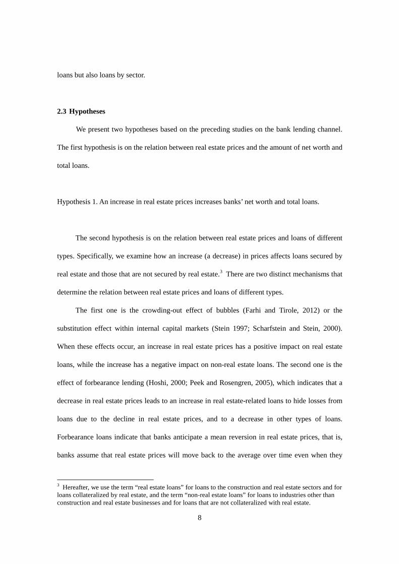
We present Figures 1 and 2 to show the heterogeneity in the PNLP real estate prices.
Figure 1 shows the heterogeneity in the real estate prices for Japanese major cities of Tokyo,
Yokohama, Kawasaki, Saitama, and Chiba. Even within a relatively small square area with
approximately 200km on each side, we observe quite sizable heterogeneity across the
municipalities in their real estate prices. Moreover, the figure substantially fluctuates from year
15

to year. By comparing the upper panel with the lower one, we see a substantial change in the
color in that the lower panel becomes “paler.” This change indicates that real estate prices in
Japan dropped substantially after the outbreak of the global financial crisis.
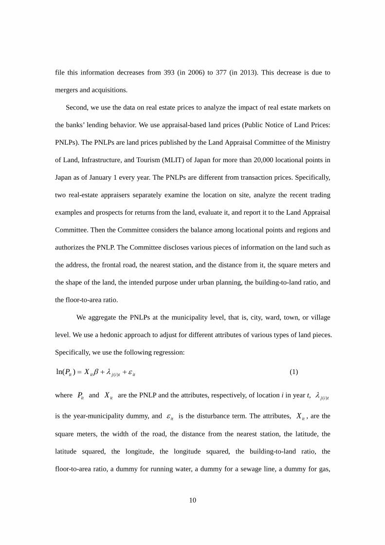
Figure 2 shows the heterogeneity in real estate prices across banks and years in Japan.
The figure emphasizes that the heterogeneity across banks as well as the fluctuations across time
appear to be quite sizable.6 The banks whose borrower firms are in metropolitan areas tend to
face higher but more volatile fluctuations in real estate prices than banks whose borrowers are in
local areas.
4.2 Effects of Real Estate Prices on Bank Loans: Bank-Level Analyses
Total loans and capital ratio
Table 3 shows the estimation results from the baseline specifications in which the
dependent variable is either the total loan-to-asset ratio (Columns 1 and 2), the log of total loans
(Columns 3 and 4), or the capital ratio (Columns 5). For the loan variable estimations, we use
either the price level (Columns 1 and 3) or its logarithm (Columns 2 and 4) as the land price
variables.
Columns 1–4 show that in the regressions of total loans, irrespective of whether they are
measured in terms of log levels or ratios to total assets, the coefficients on PRICE (Columns 1
and 3) are positive, though not significant, and those on log of PRICE (we label it as lnPRICE
hereafter) (Columns 2 and 4) are positive and significant. Column 2 shows that a one percent
increase in PRICE increases the bank’s loan-to-asset ratio by 0.06 percentage points, while
Column 4 indicates that a one percent increase in PRICE increases the bank’s total loans by 0.11
6 Note that we omit Shinkin banks from the figure due to a space constraint.
16

percent. One standard deviation in lnPRICE (0.67) increases the loan-to-asset ratio by 4.0
percentage points and the loans by 7.3 percent, both of which are economically significant.
Column 5 shows that in the regression of the capital ratio, the coefficient on lnPRICE is
positive and significant. An increase in PRICE by one percent raises the capital ratio by 0.008
percentage points, which means that a one standard deviation in lnPRICE increases the capital
ratio by 0.5 percentage points. These results show that an increase in real estate prices
substantially increases the bank’s capital and thus total loans.
The year dummies, whose reference year is 2007, peak in 2009 and turn to negative
values after 2010. This trend indicates that loans decrease both in terms of their level and ratio
to total assets from the fiscal year ending in March 2010 due to the sharp recession stemming
from the 2008 global financial crisis. The coefficient on the unemployment rate is positive and
significant. Although the positive impact of this rate on loans might be counterintuitive, this
result might reflect the demand for loans arising from the tight cash flow due to a fall in sales or
from the start-ups of new businesses.7 The log of total assets has a negative and significant
coefficient in the regressions on the loan-to-asset ratios (Columns 1 and 2), while the log of total
assets has a positive and significant coefficient in the regressions on the log of total loans
(Columns 3 and 4). These coefficients show that as assets increase, loans also increase, but to
less of an extent due to a relatively large increase in other business besides loans. The interest
rate on deposits has a positive and significant coefficient in Columns 1 and 2 that show that
banks with high interest rates, which are often small banks, have limited access to investment
opportunities other than loans and consequently increase the loan-to-asset ratio. The capital ratio
has no significant coefficients in Columns 1–4. In contrast, the capital ratio is significantly
affected by lnPRICE (Column 5), a change in capital ratios arising from the factors other than
7 Okamuro (2005) examines the factors for the start-ups of businesses in Japan and finds a positive correlation between the unemployment rate and the rate of start-ups.
17

real estate prices may not have a significant impact on loans. Finally, the net operating income
ratio has positive and significant coefficients in Columns 3 and 4.
Real estate loans and non-real estate loans
This subsection contains the results from the regressions of the real estate loans and
non-real estate loans. Table 4 shows the results from loans with and without real estate collateral,
while Table 5 shows the results from real estate loans and non-real estate loans.
Columns 1–4 of Table 4 show the results from loans collateralized by real estate. The
dependent variable is either the ratio of loans collateralized by real estates to total asset
(LOAN_COLL_r in Columns 1 and 2), or the log of loans collateralized by real estates
(lnLOAN_COLL in Columns 3 and 4). Columns 2 and 4 show that lnPRICE has positive and
significant coefficients. The PRICE also has a positive coefficient in Column 1, though not
significant. The quantitative effect of land prices on loans collateralized by real estate is also
substantial. An increase in PRICE by one percent increases the share of loans collateralized by
real estates to total assets by 0.07 percentage points (Column 2) and increases the loan amount
by 0.34 percent (Column 4), both of which are larger than the baseline results from the total
loans. Columns 5–8 in Table 4 show the results from loans without real estate collateral. The
dependent variable is either the ratio of loans not collateralized by real estates to total asset
(LOAN_NONCOLL_r in Columns 1 and 2), or the log of loans not collateralized by real estates
(lnLOAN_NONCOLL in Columns 3 and 4). They indicate that while PRICE has positive
coefficients and lnPRICE has negative coefficients, they are not significant.
Columns 1–4 in Table 5 show the results from real estate loans. The dependent variable is
either the ratio of loans to construction and real estate industries to total asset (LOAN_COLL_r
in Columns 1 and 2), or the log of loans to these industries (lnLOAN_COLL in Columns 3 and
18

4). The results indicate that PRICE and lnPRICE both have positive and significant coefficients
in all of the specifications. Column 4, for example, indicates that a one percent increase in
PRICE leads to an increase in real estate loans of 0.30 percent. But, Columns 5–8 in Table 5
show different results. The dependent variable in these columns is either the ratio of loans to
other industries to total asset (LOAN_NONRE_r in Columns 1 and 2), or the log of loans to
other industries (lnLOAN_NONRE in Columns 3 and 4). The results from non-real estate loans
indicate that although PRICE and lnPRICE have positive coefficients, they are not significant.
The results in this subsection show that an increase (a decrease) in land prices has a
positive (negative) impact on the total loans both in terms of the level and the ratio to total
assets. Thus, we infer that an increase (a decrease) in real estate prices has a positive (negative)
impact on the total loans by increasing (decreasing) the banks’ lending capacity. This inference
supports Hypothesis 1. Further, an increase (a decrease) in land prices has a significant and
relatively large impact on real estate loans, while a change in land prices does not have a
significant effect on the level of non-real estate loans. Given these results, we cannot infer that
the substitution effect actually works between these two types of loans due to a rise in lending
interest rates or through the internal capital market, which does not support Hypothesis 2.8
4.3 Effects of Real Estate Prices on Bank Loans: Matched Firm-Bank Analyses
Extensive margin
Table 6 shows the results for the extensive margin estimations represented in Eq. (4). In
addition to the results for the whole sample of firms (in Columns 1 and 2), we report those for
the real estate and construction industries (in Columns 3 and 4) and those for the other
industries (in Columns 5 and 6).
8 To test the forbearance lending in Hypothesis 2, we need an additional investigation that analyzes the effect of a fall in real estate prices by focusing on the period of their declining trend.
19
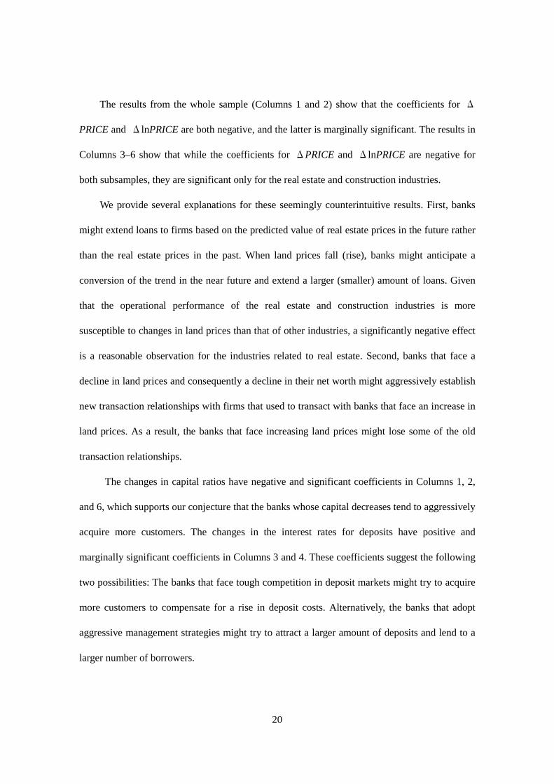
The results from the whole sample (Columns 1 and 2) show that the coefficients for Δ
PRICE and ΔlnPRICE are both negative, and the latter is marginally significant. The results in
Columns 3–6 show that while the coefficients for ΔPRICE and ΔlnPRICE are negative for
both subsamples, they are significant only for the real estate and construction industries.
We provide several explanations for these seemingly counterintuitive results. First, banks
might extend loans to firms based on the predicted value of real estate prices in the future rather
than the real estate prices in the past. When land prices fall (rise), banks might anticipate a
conversion of the trend in the near future and extend a larger (smaller) amount of loans. Given
that the operational performance of the real estate and construction industries is more
susceptible to changes in land prices than that of other industries, a significantly negative effect
is a reasonable observation for the industries related to real estate. Second, banks that face a
decline in land prices and consequently a decline in their net worth might aggressively establish
new transaction relationships with firms that used to transact with banks that face an increase in
land prices. As a result, the banks that face increasing land prices might lose some of the old
transaction relationships.
The changes in capital ratios have negative and significant coefficients in Columns 1, 2,
and 6, which supports our conjecture that the banks whose capital decreases tend to aggressively
acquire more customers. The changes in the interest rates for deposits have positive and
marginally significant coefficients in Columns 3 and 4. These coefficients suggest the following
two possibilities: The banks that face tough competition in deposit markets might try to acquire
more customers to compensate for a rise in deposit costs. Alternatively, the banks that adopt
aggressive management strategies might try to attract a larger amount of deposits and lend to a
larger number of borrowers.
20
Intensive margin
Table 7 shows the results for the intensive margin estimations from Eq. (5). We report the
results for the whole sample of firms (in Columns 1 and 2), those for the real estate and
construction industries (in Columns 3 and 4), and those for the other industries (in Columns 5
and 6).
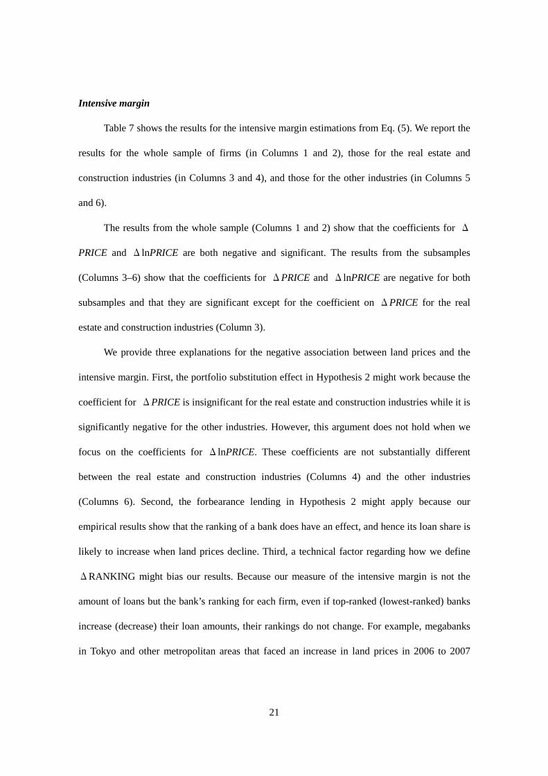
The results from the whole sample (Columns 1 and 2) show that the coefficients for Δ
PRICE and ΔlnPRICE are both negative and significant. The results from the subsamples
(Columns 3–6) show that the coefficients for ΔPRICE and ΔlnPRICE are negative for both
subsamples and that they are significant except for the coefficient on ΔPRICE for the real
estate and construction industries (Column 3).
We provide three explanations for the negative association between land prices and the
intensive margin. First, the portfolio substitution effect in Hypothesis 2 might work because the
coefficient for ΔPRICE is insignificant for the real estate and construction industries while it is
significantly negative for the other industries. However, this argument does not hold when we
focus on the coefficients for ΔlnPRICE. These coefficients are not substantially different
between the real estate and construction industries (Columns 4) and the other industries
(Columns 6). Second, the forbearance lending in Hypothesis 2 might apply because our
empirical results show that the ranking of a bank does have an effect, and hence its loan share is
likely to increase when land prices decline. Third, a technical factor regarding how we define
ΔRANKING might bias our results. Because our measure of the intensive margin is not the
amount of loans but the bank’s ranking for each firm, even if top-ranked (lowest-ranked) banks
increase (decrease) their loan amounts, their rankings do not change. For example, megabanks
in Tokyo and other metropolitan areas that faced an increase in land prices in 2006 to 2007
21

might have increased loans during this period. However, they were top-ranked for a number of
firms and hence their ranking might not have changed.
We find that changes in the capital ratio have negative and significant coefficients in
Columns 1–6, while changes in interest rates have positive and marginally significant
coefficients in Columns 1, 2, 5, and 6. These results are qualitatively similar to those for the
extensive margin estimation. In addition, the changes in assets have a negative and marginally
significant coefficient in Column 3.
Thus, we find that an increase in land prices has a significantly negative impact on the
evolution of bank-firm relationships. Specifically, a bank that faces an increase in land prices
not only reduces the number of relationships with firms but also moves down in the order of
importance on the list of the banks that the firm borrows from. This finding does not support
Hypothesis 1 and is the opposite in sign from the results in the previous subsection.
5 Discussion and Conclusion
We examine the effect of real estate price shocks on the bank lending channel and the
substitution effect on real estate loans and non-real estate loans (Chakraborty et al., 2014; Cuñat
et al., 2014). Using Japanese data in the 2007–2013 global financial crisis, we identify
heterogeneous real estate price shocks that affect each bank by summarizing the land prices of
firms with which the bank has transaction relationships. Using bank-level data and controlling
for bank fixed effects, we obtain evidence that is overall in line with the prediction of the bank
lending channel in that a rise in land prices increases banks’ capital and total bank loans.
However, our bank-level estimation, even though it uses variables for regional and
macroeconomic activities, is not enough to control for the factors that affect loan availability for
individual firms, especially those that are related to the change in real estate prices. In order to
22

precisely identify the impact of real estate prices on a bank’s loan supply, we use a matched
firm-bank data set. After controlling for firms’ time-varying fixed effects, we find that a bank
that faces an increase in land prices not only reduces the number of relationships with firms but
also moves down on the list of the banks that the firm transacts with. This finding does not
support the hypothesis of the bank lending channel and contradicts the bank-level estimation
results. While we do not identify a precise mechanism for the negative impact of land prices on
the loan supply, we leave this to future work. However, our findings indicate that we need to
modify our overly simplistic view on the function of the bank lending channel in real estate
prices, that is, a bank that experiences an increase in real estate prices immediately increases its
loan supply.
23
References Bernanke, B.S. (1983) “Nonmonetary Effects of the Financial Crisis in the Propagation of the Great Depression,” American Economic Review, 73, pp. 257-276. Bernanke, B. and M. Gertler (1989) “Agency Costs, Net Worth, and Business Fluctuations,” American Economic Review, 79 (1), pp. 14-31. Chakraborty, I., I. Goldstein, and A. MacKinlay (2014) “Do asset price booms have negative real effects?” Working Paper. Chaney, T., D. Sraer, and D. Thesmar (2012) “The collateral channel: How real estate shocks affect corporate investment, American Economic Review, 102(6), pp. 2381-2409. Cuñat, V., D. Cvijanović, and K. Yuan (2014) “Within-bank transmission of real estate shocks,” Working Paper. Farhi, E. and J. Tirole (2012) “Bubbly liquidity,” Review of Economic Studies, 79, pp. 678-706. Gan, J. (2007a) “Collateral, debt capacity, and corporate investment: Evidence from a natural experiment,” Journal of Financial Economics, 85, pp. 709-734. Gan, J. (2007b) “The real effects of asset market bubbles: loan- and firm-level evidence of a lending channel,” Review of Financial Studies, 20(5), pp. 1941-1973. Holmström, B. and J. Tirole (1997) “Financial Intermediation, Loanable Funds, and the Real Sector,” Quarterly Journal of Economics, 112(3), pp. 663-691. Hoshi, T. (2000) “Why cannot Japan escape from the liquidity trap,” (in Japanese) M. Fukao and H. Yoshikawa eds, The Zero Interest Rate and the Japanese Economy, Nihon Keizai Shinbun sha. Hosono, K. and D. Miyakawa (2014) “Bank Lending and Firm Activities: Overcoming Identification Problems,” T. Watanabe, I. Uesugi, A. Ono eds, The Economics of Interfirm Networks, Chapter 12, Springer, forthcoming. Hosono, K., D. Miyakawa, T. Uchino, M. Hazama, A. Ono, H. Uchida, and I. Uesugi (2012) “Natural Disasters, Damage to Banks, and Firm Investment,” RIETI Discussion Paper Series 12-E-062. Miyakawa, D., K. Hosono, T. Uchino, A. Ono, H. Uchida, and I. Uesugi (2014) “Natural Disasters, Financial Shocks, and Firm Export,” RIETI Discussion Paper 14-E-010. Ogawa, K. (2003) Economic Analysis of the Great Depression, Nippon Keizai Shinbun sha. Ogawa, K., S. Kitasaka, H. Yamaoka, and Y. Iwata (1996) “Borrowing constraints and the role of land asset in Japanese corporate investment decision,” Journal of the Japanese and International Economies 10 (2), pp. 122-149. Ogawa, K. and K. Suzuki (1998) “Land value and corporate investment: evidence from Japanese panel data,” Journal of the Japanese and International Economies 12 (3), pp. 232-249.
24
Okamuro, H. “Regional factors for the start-up rats of manufacturing firms: A comparative analysis between high-tech and low-tech industries,” (in Japanese) RIETI Discussion Paper Series 06-J-049. Paravisini, D. (2008) “Local bank financial constraints and firm access to external finance,” Journal of Finance, 63, pp. 2161-2193. Peek, J. and E.S. Rosengren (1997) “The International Transmission of Financial Shocks: The Case of Japan,” American Economic Review, 87(4), pp. 495-505. Peek, J. and E.S. Rosengren (2000) “Collateral Damage: Effects of the Japanese Bank Crisis on Real Activity in the United States,” American Economic Review, 90, pp. 30-45. Peek, J. and E.S. Rosengren (2005) “Unnatural Selection: Perverse Incentives and the Misallocation of Credit in Japan,” American Economic Review, 95, pp. 1144-1166. Puri, M., J. Rocholl, and S. Steffen (2011) “Global retail lending in the aftermath of the US financial crisis: Distinguishing between supply and demand effects,” Journal of Financial Economics, 100, pp. 556-578. Scharfstein, D.S. and J.C. Stein (2000) “The dark side of internal capital markets: Divisional rent-seeking and inefficient investment,” Journal of Finance, 55, pp. 2537-2564. Schnabl, P. (2012) “The International Transmission of Bank Liquidity Shocks: Evidence from an Emerging Market,” Journal of Finance, 67, pp. 897-932. Stein, J.C. (1997) “Internal capital markets and the competition for corporate resources,” Journal of Finance, 52, pp. 111-133. Stiglitz, J.E. and A. Weiss (1981) “Credit rationing in markets with imperfect information,” American Economic Review, 71, pp. 393-410. Tokumitsu, S. (2006) A Guide for the Evaluation of Collateral (in Japanese), Kinyu-Zaisei Jijo Kenkyukai, Tokyo.
25

Table 1. Definitions and descriptive statistics of variables
Variable names Definitions N mean sd min p25 p50 p75 maxDependent variables
Total loan amount
LOAN_r Total loan amount outstanding/Totalasset
2647 0.5502 0.1256 0.0744 0.4639 0.5409 0.6413 1.5624
lnLOAN ln(Total loan amount outstanding) (Unitof loan amount outstanding: million yen)
2647 12.5720 1.5206 9.2460 11.3640 12.3364 13.7027 18.1210
Loans related to real estate
LOAN_COLL_r Amount of loans collateralized by realestate/Total asset
2635 0.1613 0.0932 0.0000 0.0973 0.1511 0.2123 0.7856
lnLOAN_COLL ln(Amount of loans collateralized by realestate) (Unit: million yen)
2499 11.1853 1.3959 7.7890 10.1403 11.0674 12.1188 15.7465
LOAN_RE_r Amount of loans to construction andreal estate industries/Total asset
2647 0.1225 0.0562 0.0000 0.0849 0.1142 0.1523 0.4355
lnLOAN_RE ln(Amount of loans to construction andreal estate industries) (Unit: million yen)
2597 11.0145 1.5069 7.4657 9.9163 10.9187 12.0895 16.1279
Loans not related to real estate
LOAN_NONCOLL_r Amount of loans not collateralized byreal estate/Total asset
2635 0.3883 0.1336 0.0744 0.3021 0.3630 0.4640 1.1745
lnLOAN_NONCOLL ln(Amount of loans not collateralized byreal estate) (Unit: million yen)
2635 12.1824 1.5945 8.6620 10.9040 11.9012 13.3266 18.0412
LOAN_NONRE_r Amount of loans to otherindustries/Total asset
2647 0.4277 0.1173 0.0669 0.3452 0.4090 0.5088 1.1828
lnLOAN_NONRE ln(Amount of loans to other industries)(Unit: million yen)
2647 12.3103 1.5417 9.0614 11.0553 12.0325 13.4212 17.9909
Capital ratioB_CAPRATIO Capital ratio 2647 0.0533 0.0197 0.0035 0.0397 0.0501 0.0633 0.1710
Explanatory variables (all the variables are lagged by one year)Real estate prices
PRICE Public notice of land price (公示地価)(Unit: yen per square meter)
2647 33006.51 31225.08 7711.324 15707.97 21381.89 34582.48 208020.5
lnPRICE ln(public notice of land price) 2647 10.1326 0.6690 8.9504 9.6619 9.9703 10.4511 12.2454Bank characteristics
lnB_ASSET ln(bank's total asset) 2647 13.1978 1.4115 10.5242 12.0920 13.0019 14.1671 18.8997B_CAPRATIO Capital ratio 2647 0.0533 0.0197 0.0035 0.0397 0.0501 0.0633 0.1710B_ROA Business profit(業務純益)/Total asset 2647 0.0014 0.0052 -0.0649 0.0010 0.0021 0.0036 0.0300
B_DEPOSITCOST Interest payment amount todeposits/Deposits
2647 0.0020 0.0012 0.0002 0.0010 0.0017 0.0027 0.0207
Local economic conditions
UNEMPUnemployment rate in the prefectureswhere bank branches are located (Unit:%)
2647 4.2384 0.9023 2.2000 3.6099 4.2000 4.8000 7.6000
26
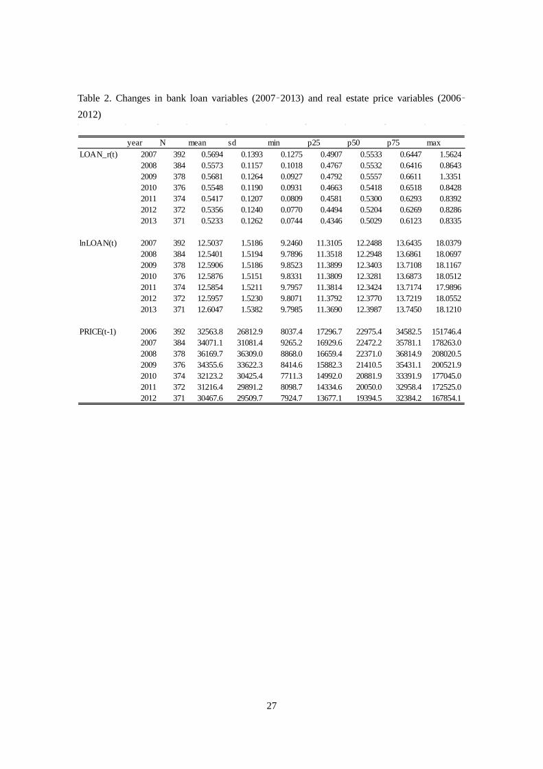
Table 2. Changes in bank loan variables (2007–2013) and real estate price variables (2006–2012)
year N mean sd min p25 p50 p75 maxLOAN_r(t) 2007 392 0.5694 0.1393 0.1275 0.4907 0.5533 0.6447 1.5624
2008 384 0.5573 0.1157 0.1018 0.4767 0.5532 0.6416 0.86432009 378 0.5681 0.1264 0.0927 0.4792 0.5557 0.6611 1.33512010 376 0.5548 0.1190 0.0931 0.4663 0.5418 0.6518 0.84282011 374 0.5417 0.1207 0.0809 0.4581 0.5300 0.6293 0.83922012 372 0.5356 0.1240 0.0770 0.4494 0.5204 0.6269 0.82862013 371 0.5233 0.1262 0.0744 0.4346 0.5029 0.6123 0.8335
lnLOAN(t) 2007 392 12.5037 1.5186 9.2460 11.3105 12.2488 13.6435 18.03792008 384 12.5401 1.5194 9.7896 11.3518 12.2948 13.6861 18.06972009 378 12.5906 1.5186 9.8523 11.3899 12.3403 13.7108 18.11672010 376 12.5876 1.5151 9.8331 11.3809 12.3281 13.6873 18.05122011 374 12.5854 1.5211 9.7957 11.3814 12.3424 13.7174 17.98962012 372 12.5957 1.5230 9.8071 11.3792 12.3770 13.7219 18.05522013 371 12.6047 1.5382 9.7985 11.3690 12.3987 13.7450 18.1210
PRICE(t-1) 2006 392 32563.8 26812.9 8037.4 17296.7 22975.4 34582.5 151746.42007 384 34071.1 31081.4 9265.2 16929.6 22472.2 35781.1 178263.02008 378 36169.7 36309.0 8868.0 16659.4 22371.0 36814.9 208020.52009 376 34355.6 33622.3 8414.6 15882.3 21410.5 35431.1 200521.92010 374 32123.2 30425.4 7711.3 14992.0 20881.9 33391.9 177045.02011 372 31216.4 29891.2 8098.7 14334.6 20050.0 32958.4 172525.02012 371 30467.6 29509.7 7924.7 13677.1 19394.5 32384.2 167854.1
27
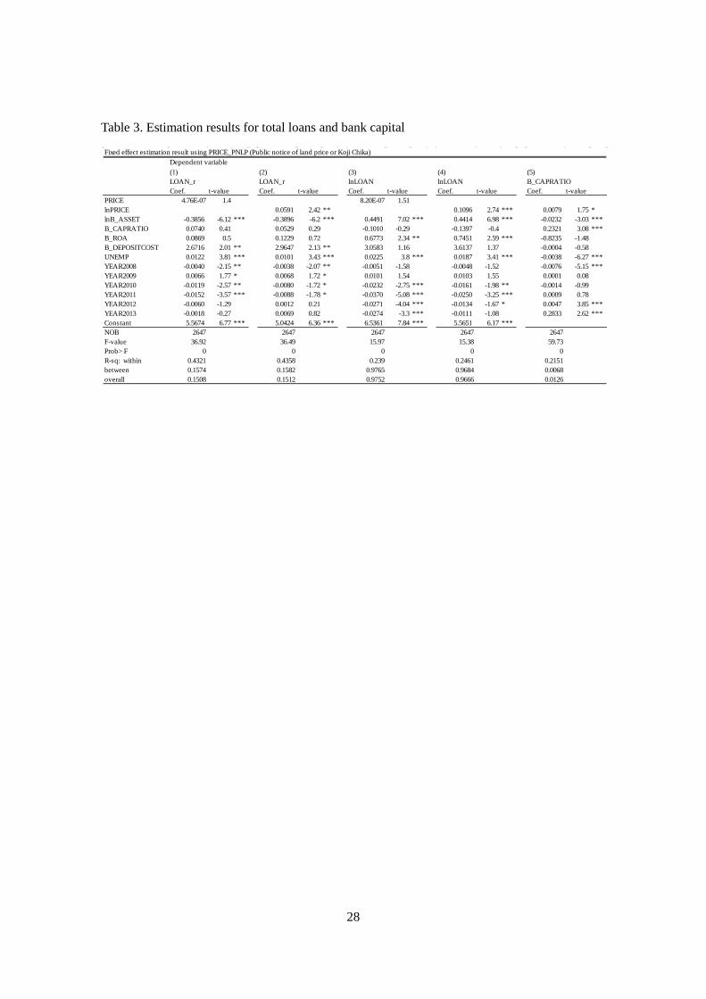
Table 3. Estimation results for total loans and bank capital
Fixed effect estimation result using PRICE_PNLP (Public notice of land price or Koji Chika)Dependent variable(1) (2) (3) (4) (5)LOAN_r LOAN_r lnLOAN lnLOAN B_CAPRATIOCoef. t-value Coef. t-value Coef. t-value Coef. t-value Coef. t-value
PRICE 4.76E-07 1.4 8.20E-07 1.51lnPRICE 0.0591 2.42 ** 0.1096 2.74 *** 0.0079 1.75 *lnB_ASSET -0.3856 -6.12 *** -0.3896 -6.2 *** 0.4491 7.02 *** 0.4414 6.98 *** -0.0232 -3.03 ***B_CAPRATIO 0.0740 0.41 0.0529 0.29 -0.1010 -0.29 -0.1397 -0.4 0.2321 3.08 ***B_ROA 0.0869 0.5 0.1229 0.72 0.6773 2.34 ** 0.7451 2.59 *** -0.8235 -1.48B_DEPOSITCOST 2.6716 2.01 ** 2.9647 2.13 ** 3.0583 1.16 3.6137 1.37 -0.0004 -0.58UNEMP 0.0122 3.81 *** 0.0101 3.43 *** 0.0225 3.8 *** 0.0187 3.41 *** -0.0038 -6.27 ***YEAR2008 -0.0040 -2.15 ** -0.0038 -2.07 ** -0.0051 -1.58 -0.0048 -1.52 -0.0076 -5.15 ***YEAR2009 0.0066 1.77 * 0.0068 1.72 * 0.0101 1.54 0.0103 1.55 0.0001 0.08YEAR2010 -0.0119 -2.57 ** -0.0080 -1.72 * -0.0232 -2.75 *** -0.0161 -1.98 ** -0.0014 -0.99YEAR2011 -0.0152 -3.57 *** -0.0088 -1.78 * -0.0370 -5.08 *** -0.0250 -3.25 *** 0.0009 0.78YEAR2012 -0.0060 -1.29 0.0012 0.21 -0.0271 -4.04 *** -0.0134 -1.67 * 0.0047 3.85 ***YEAR2013 -0.0018 -0.27 0.0069 0.82 -0.0274 -3.3 *** -0.0111 -1.08 0.2833 2.62 ***Constant 5.5674 6.77 *** 5.0424 6.36 *** 6.5361 7.84 *** 5.5651 6.17 ***NOB 2647 2647 2647 2647 2647F-value 36.92 36.49 15.97 15.38 59.73Prob> F 0 0 0 0 0R-sq: within 0.4321 0.4358 0.239 0.2461 0.2151between 0.1574 0.1582 0.9765 0.9684 0.0068overall 0.1508 0.1512 0.9752 0.9666 0.0126
28
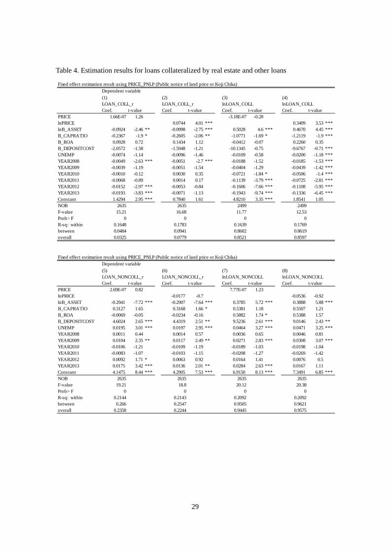
Table 4. Estimation results for loans collateralized by real estate and other loans
Fixed effect estimation result using PRICE_PNLP (Public notice of land price or Koji Chika)Dependent variable(1) (2) (3) (4)LOAN_COLL_r LOAN_COLL_r lnLOAN_COLL lnLOAN_COLLCoef. t-value Coef. t-value Coef. t-value Coef. t-value
PRICE 1.66E-07 1.26 -3.18E-07 -0.28lnPRICE 0.0744 4.01 *** 0.3409 3.53 ***lnB_ASSET -0.0924 -2.46 ** -0.0998 -2.75 *** 0.5028 4.6 *** 0.4670 4.45 ***B_CAPRATIO -0.2367 -1.9 * -0.2605 -2.06 ** -1.0771 -1.69 * -1.2119 -1.9 ***B_ROA 0.0928 0.72 0.1434 1.12 -0.0412 -0.07 0.2260 0.35B_DEPOSITCOST -2.0572 -1.58 -1.5948 -1.21 -10.1345 -0.75 -9.6767 -0.71 ***UNEMP -0.0074 -1.14 -0.0096 -1.46 -0.0109 -0.58 -0.0200 -1.18 ***YEAR2008 -0.0049 -2.63 *** -0.0051 -2.7 *** -0.0188 -1.52 -0.0185 -1.53 ***YEAR2009 -0.0039 -1.19 -0.0051 -1.54 -0.0404 -1.29 -0.0439 -1.42 ***YEAR2010 -0.0010 -0.12 0.0030 0.35 -0.0721 -1.84 * -0.0506 -1.4 ***YEAR2011 -0.0068 -0.89 0.0014 0.17 -0.1139 -3.79 *** -0.0725 -2.81 ***YEAR2012 -0.0152 -2.97 *** -0.0053 -0.84 -0.1606 -7.66 *** -0.1108 -5.95 ***YEAR2013 -0.0193 -3.83 *** -0.0071 -1.13 -0.1943 -9.74 *** -0.1336 -6.45 ***Constant 1.4294 2.95 *** 0.7840 1.61 4.8210 3.35 *** 1.8541 1.05NOB 2635 2635 2499 2499F-value 15.21 16.68 11.77 12.53Prob> F 0 0 0 0R-sq: within 0.1648 0.1783 0.1639 0.1769between 0.0484 0.0941 0.8602 0.8619overall 0.0325 0.0779 0.8521 0.8597
Fixed effect estimation result using PRICE_PNLP (Public notice of land price or Koji Chika)Dependent variable(5) (6) (7) (8)LOAN_NONCOLL_r LOAN_NONCOLL_r lnLOAN_NONCOLL lnLOAN_NONCOLLCoef. t-value Coef. t-value Coef. t-value Coef. t-value
PRICE 2.69E-07 0.82 7.77E-07 1.23lnPRICE -0.0177 -0.7 -0.0536 -0.92lnB_ASSET -0.2941 -7.72 *** -0.2907 -7.64 *** 0.3785 5.72 *** 0.3888 5.88 ***B_CAPRATIO 0.3127 1.65 0.3168 1.66 * 0.5381 1.18 0.5507 1.21B_ROA -0.0069 -0.05 -0.0234 -0.16 0.5882 1.74 * 0.5388 1.57B_DEPOSITCOST 4.6024 2.65 *** 4.4319 2.51 ** 9.5236 2.61 *** 9.0146 2.43 **UNEMP 0.0195 3.01 *** 0.0197 2.95 *** 0.0464 3.27 *** 0.0471 3.25 ***YEAR2008 0.0011 0.44 0.0014 0.57 0.0036 0.65 0.0046 0.81YEAR2009 0.0104 2.35 ** 0.0117 2.49 ** 0.0271 2.83 *** 0.0308 3.07 ***YEAR2010 -0.0106 -1.21 -0.0109 -1.19 -0.0189 -1.03 -0.0198 -1.04YEAR2011 -0.0083 -1.07 -0.0103 -1.15 -0.0208 -1.27 -0.0269 -1.42YEAR2012 0.0092 1.71 * 0.0063 0.92 0.0164 1.41 0.0076 0.5YEAR2013 0.0175 3.42 *** 0.0136 2.01 ** 0.0284 2.63 *** 0.0167 1.11Constant 4.1475 8.44 *** 4.2905 7.53 *** 6.9150 8.13 *** 7.3491 6.85 ***NOB 2635 2635 2635 2635F-value 19.21 18.8 20.12 20.38Prob> F 0 0 0 0R-sq: within 0.2144 0.2143 0.2092 0.2092between 0.266 0.2547 0.9505 0.9621overall 0.2358 0.2244 0.9445 0.9575
29

Table 5. Estimation results for loans to construction and real estate industries and loans to others.
Fixed effect estimation result using PRICE_PNLP (Public notice of land price or Koji Chika)Dependent variable(1) (2) (3) (4)LOAN_RE_r LOAN_RE_r lnLOAN_RE lnLOAN_RECoef. t-value Coef. t-value Coef. t-value Coef. t-value
PRICE 4.46E-07 2.48 ** 2.85E-06 2.82 ***lnPRICE 0.0291 1.84 * 0.3021 3.77 ***lnB_ASSET -0.0938 -4.3 *** -0.0946 -4.36 *** 0.4700 5.34 *** 0.4550 5.3 ***B_CAPRATIO 0.1124 1.16 0.1008 1.01 -0.1905 -0.34 -0.3216 -0.56B_ROA -0.0394 -0.28 -0.0249 -0.18 0.3400 0.64 0.5131 0.97B_DEPOSITCOST -1.0215 -1.03 -0.9178 -0.96 -11.2349 -1.12 -9.8294 -1UNEMP 0.0051 1.38 0.0039 1.04 0.0225 1.51 0.0113 0.78YEAR2008 0.0025 1.74 * 0.0027 1.94 * 0.0109 1.22 0.0122 1.38YEAR2009 0.0068 2.63 *** 0.0076 3.02 *** 0.0402 1.72 * 0.0425 1.83 *YEAR2010 0.0046 0.93 0.0070 1.4 0.0598 2.06 ** 0.0807 2.8 ***YEAR2011 0.0038 0.87 0.0069 1.39 0.0411 1.69 * 0.0737 2.95 ***YEAR2012 0.0043 1.28 0.0075 1.73 * 0.0325 1.87 * 0.0689 3.57 ***YEAR2013 0.0065 1.96 * 0.0101 2.23 ** 0.0297 1.72 * 0.0725 3.63 ***Constant 1.3164 4.63 *** 1.0502 3.11 *** 4.6291 4.03 *** 1.8941 1.34NOB 2647 2647 2597 2597F-value 6.53 6.64 10.75 11.42Prob> F 0 0 0 0R-sq: within 0.0638 0.063 0.1206 0.1291between 0.0004 0.0014 0.9307 0.9196overall 0.0003 0.0012 0.9263 0.9172
Fixed effect estimation result using PRICE_PNLP (Public notice of land price or Koji Chika)Dependent variable(5) (6) (7) (8)LOAN_NONRE_r LOAN__NONRE_r lnLOAN_NONRE lnLOAN_NONRECoef. t-value Coef. t-value Coef. t-value Coef. t-value
PRICE 3.00E-08 0.1 1.05E-07 0.17lnPRICE 0.0300 1.16 0.0413 0.77lnB_ASSET -0.2918 -5.73 *** -0.2950 -5.83 *** 0.4633 6.22 *** 0.4592 6.22 ***B_CAPRATIO -0.0383 -0.2 -0.0478 -0.24 -0.3014 -0.71 -0.3149 -0.73B_ROA 0.1263 0.66 0.1478 0.78 0.8333 2.09 ** 0.8619 2.17 **B_DEPOSITCOST 3.6930 2.3 ** 3.8825 2.38 ** 5.8821 2.15 ** 6.1306 2.21 **UNEMP 0.0071 1.66 * 0.0062 1.48 0.0165 1.84 * 0.0153 1.75 *YEAR2008 -0.0064 -3.33 *** -0.0066 -3.35 *** -0.0135 -3.47 *** -0.0136 -3.48 ***YEAR2009 -0.0003 -0.06 -0.0009 -0.19 -0.0022 -0.29 -0.0028 -0.37YEAR2010 -0.0165 -2.51 ** -0.0150 -2.31 ** -0.0396 -3.21 *** -0.0374 -3.1 ***YEAR2011 -0.0190 -3.48 *** -0.0157 -2.53 ** -0.0541 -5.17 *** -0.0495 -4.21 ***YEAR2012 -0.0103 -2.2 ** -0.0063 -1.03 -0.0428 -4.76 *** -0.0373 -3.22 ***YEAR2013 -0.0083 -1.45 -0.0032 -0.43 -0.0469 -4.59 *** -0.0401 -2.93 ***Constant 4.2510 6.41 *** 3.9922 5.74 *** 6.1543 6.34 *** 5.7957 5.15 ***NOB 2647 2647 2647 2647F-value 30.43 30.14 13.53 13.54Prob> F 0 0 0 0R-sq: within 0.3082 0.3097 0.1422 0.1431between 0.1745 0.1823 0.9736 0.9695overall 0.1623 0.1702 0.971 0.9667
30
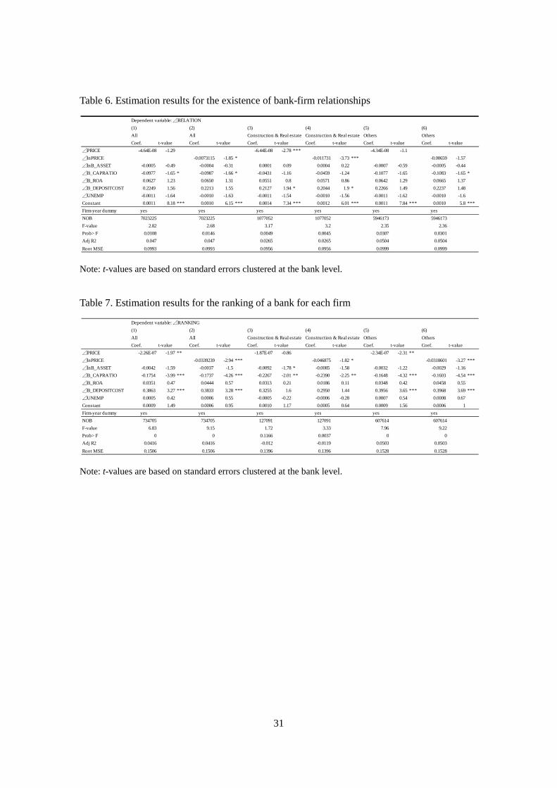
Table 6. Estimation results for the existence of bank-firm relationships
Note: t-values are based on standard errors clustered at the bank level.
Table 7. Estimation results for the ranking of a bank for each firm
Note: t-values are based on standard errors clustered at the bank level.
Dependent variable: ⊿RELATION(1) (2) (3) (4) (5) (6)All All Construction & Real estate Construction & Real estate Others OthersCoef. t-value Coef. t-value Coef. t-value Coef. t-value Coef. t-value Coef. t-value
⊿PRICE -4.64E-08 -1.29 -6.44E-08 -2.78 *** -4.34E-08 -1.1⊿lnPRICE -0.0073115 -1.85 * -0.011731 -3.73 *** -0.00659 -1.57⊿lnB_ASSET -0.0005 -0.49 -0.0004 -0.31 0.0001 0.09 0.0004 0.22 -0.0007 -0.59 -0.0005 -0.44⊿B_CAPRATIO -0.0977 -1.65 * -0.0987 -1.66 * -0.0431 -1.16 -0.0459 -1.24 -0.1077 -1.65 -0.1083 -1.65 *⊿B_ROA 0.0627 1.23 0.0650 1.31 0.0551 0.8 0.0571 0.86 0.0642 1.29 0.0665 1.37⊿B_DEPOSITCOST 0.2249 1.56 0.2213 1.55 0.2127 1.94 * 0.2044 1.9 * 0.2266 1.49 0.2237 1.48⊿UNEMP -0.0011 -1.64 -0.0010 -1.63 -0.0011 -1.54 -0.0010 -1.56 -0.0011 -1.62 -0.0010 -1.6Constant 0.0011 8.18 *** 0.0010 6.15 *** 0.0014 7.34 *** 0.0012 6.01 *** 0.0011 7.84 *** 0.0010 5.8 ***Firm-year dummy yes yes yes yes yes yesNOB 7023225 7023225 1077052 1077052 5946173 5946173F-value 2.82 2.68 3.17 3.2 2.35 2.36Prob> F 0.0108 0.0146 0.0049 0.0045 0.0307 0.0301Adj R2 0.047 0.047 0.0265 0.0265 0.0504 0.0504Root MSE 0.0993 0.0993 0.0956 0.0956 0.0999 0.0999
Dependent variable: ⊿RANKING(1) (2) (3) (4) (5) (6)All All Construction & Real estate Construction & Real estate Others OthersCoef. t-value Coef. t-value Coef. t-value Coef. t-value Coef. t-value Coef. t-value
⊿PRICE -2.26E-07 -1.97 ** -1.87E-07 -0.86 -2.34E-07 -2.31 **⊿lnPRICE -0.0339239 -2.94 *** -0.046875 -1.82 * -0.0318601 -3.27 ***⊿lnB_ASSET -0.0042 -1.59 -0.0037 -1.5 -0.0092 -1.78 * -0.0085 -1.58 -0.0032 -1.22 -0.0029 -1.16⊿B_CAPRATIO -0.1754 -3.99 *** -0.1737 -4.26 *** -0.2267 -2.01 ** -0.2390 -2.25 ** -0.1648 -4.32 *** -0.1603 -4.54 ***⊿B_ROA 0.0351 0.47 0.0444 0.57 0.0313 0.21 0.0186 0.11 0.0348 0.42 0.0458 0.55⊿B_DEPOSITCOST 0.3863 3.27 *** 0.3833 3.28 *** 0.3255 1.6 0.2950 1.44 0.3956 3.65 *** 0.3968 3.69 ***⊿UNEMP 0.0005 0.42 0.0006 0.55 -0.0005 -0.22 -0.0006 -0.28 0.0007 0.54 0.0008 0.67Constant 0.0009 1.49 0.0006 0.95 0.0010 1.17 0.0005 0.64 0.0009 1.56 0.0006 1Firm-year dummy yes yes yes yes yes yesNOB 734705 734705 127091 127091 607614 607614F-value 6.83 9.15 1.72 3.33 7.96 9.22Prob> F 0 0 0.1166 0.0037 0 0Adj R2 0.0416 0.0416 -0.012 -0.0119 0.0503 0.0503Root MSE 0.1506 0.1506 0.1396 0.1396 0.1528 0.1528
31

Figure 1. Spatial distributions of real estate prices for municipalities in 2008 and 2009 (Areas that include entire prefectures of Tokyo, Kanagawa, Saitama, and Chiba)
Year 2008
Year 2009
Note: For each local municipality, we use different colors for different real estate price ranges for 2008 and 2009. Areas without color indicate no reporting locations for PNLP. The unit of measurement is the yen.
32
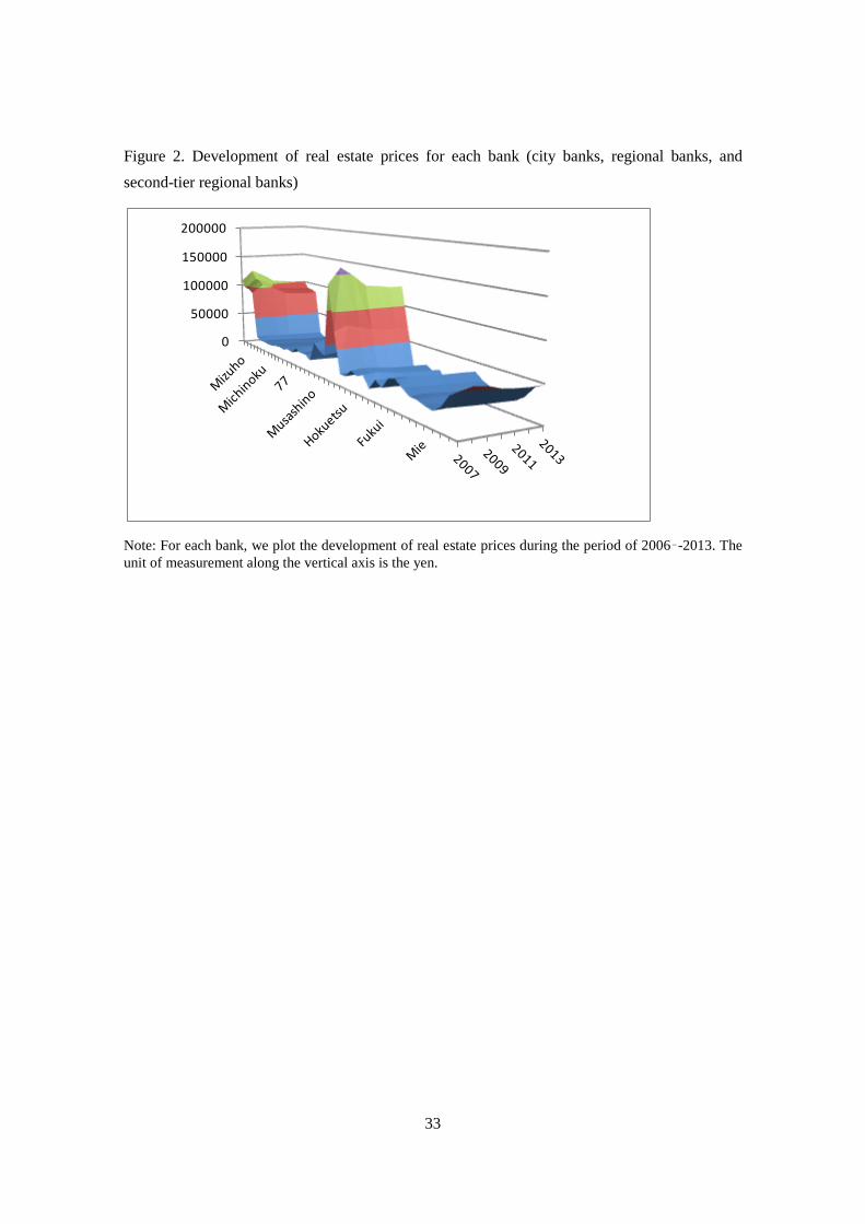
Figure 2. Development of real estate prices for each bank (city banks, regional banks, and second-tier regional banks)
Note: For each bank, we plot the development of real estate prices during the period of 2006–-2013. The unit of measurement along the vertical axis is the yen.
0
50000
100000
150000
200000
33