THE OREGON PLAN for Salmon and Watersheds

Year 2000 Stream Habitat Conditions in Western Oregon Report Number: OPSW-ODFW-2001-05

YEAR 2000 STREAM HABITAT

CONDITIONS IN WESTERN OREGON

Oregon Plan for Salmon and Watersheds

Monitoring report No. OPSW-ODFW-2001-05

March 11, 2002

Rebecca Flitcroft Kim Jones Kelly Reis

Barry Thom

Aquatic Inventories Project Oregon Department of Fish and Wildlife

28655 Highway 34 Corvallis, OR 97333

Funds supplied in part by: State of Oregon (OPSW), Oregon Forest Industries Council Citation: Flitcroft, R.L., K.K. Jones, K.E.M. Reis, and B.A. Thom. 2002. Year 2000 stream habitat conditions in western Oregon. Monitoring Program Report Number OPSW-ODFW-2001-05, Oregon Department of Fish and Wildlife, Portland.

ii

iii

CONTENTS

FIGURES..................................................................................................................................... IV

TABLES........................................................................................................................................ V

INTRODUCTION......................................................................................................................... 1

METHODS .................................................................................................................................... 4 STUDY AREA AND SITE SELECTION ............................................................................................. 4 SURVEY METHODS....................................................................................................................... 5 ANALYSIS .................................................................................................................................... 6

Overall Habitat Conditions..................................................................................................... 6 Habitat Condition and Quality 1998-2000............................................................................. 7 Trends in habitat quality 1998 – 2000.................................................................................... 8 Habitat Resurvey..................................................................................................................... 8

RESULTS AND DISCUSSION ................................................................................................... 9 HABITAT CONDITIONS FOR 2000.................................................................................................. 9 FISH SURVEYS............................................................................................................................ 17 TRENDS 1998-2000.................................................................................................................... 21 RESURVEY ANALYSIS ................................................................................................................ 25

CONCLUSIONS ......................................................................................................................... 27

ACKNOWLEDGEMENTS ....................................................................................................... 28

REFERENCES............................................................................................................................ 29

APPENDICES............................................................................................................................. 31 APPENDIX 1: ODFW BENCHMARKS .......................................................................................... 31 APPENDIX 2: CUMULATIVE DISTRIBUTIONS OF FREQUENCY FOR 1998, 1999 AND 2000 ............ 35

iv

FIGURES

Number Page Figure 1. Map of Oregon Plan Habitat Monitoring Program sites 1998-2000……………………4 Figure 2. Map and cumulative distribution of frequency graphs showing Oregon Plan sites for 2000 displaying percent pool habitat and percent gravel in riffles………………………………13 Figure 3. Map and cumulative distribution of frequency graphs showing Oregon Plan sites for 2000 displaying the volume of large woody debris and the density of riparian conifers………..14 Figure 4. Map and cumulative distribution of frequency graphs showing Oregon Plan sites for 2000 displaying deep pools (>1.0m) and percent fines in riffle units…………………………...15 Figure 5. Map and cumulative distribution of frequency graphs showing Oregon Plan sites for 2000 displaying the volume of large woody debris (>1.0m dbh) and the density of large riparian conifers (>1.0m dbh)……………………………………………………………………………..16 Figure 6. Map of sites for 2000 where coho were found outside their expected distribution…...17 Figure 7. Box plots displaying composite data by year for selected variables……………….19-20 Figure 8. Cumulative frequency distribution graph for large riparian conifer counts in 1998, 1999 and 2000………………………………………………………………………………………….21 Figure 9. Map of sites for 1998-2000 showing sites outside the expected distribution of coho that exceeded a variety of ODFW’s benchmark criteria.…………………………………………….23 Figure 10. Map of sites for 1998-2000 showing sites within the expected distribution of coho that exceeded a variety of ODFW’s benchmark criteria.……………………………………………..24

v

TABLES

Number Page Table 1. Summary of sites selected in year 2000……………...………………………………….5 Table 2. Variables collected for year 2000 sites averaged by coho distribution criteria………….9 Table 3. Cumulative frequency distribution quartiles and summary statistics for fines and gravel in riffle units……………………………………………………………………………………...10 Table 4. Cumulative frequency distribution quartiles and summary statistics for pool units……10 Table 5. Cumulative frequency distribution quartiles and summary statistics for woody debris metrics..…………………………………………………………………………………………..11 Table 6. Cumulative frequency distribution quartiles and summary statistics for riparian conifers…………………………………………………………………………………………...12 Table 7. Summary statistics for sites surveyed outside the distribution of coho but where coho salmon were sampled……..……………………………………………………………………...17 Table 8. Benchmark summary table showing the percent of sites that exceeded at least three benchmark criteria……………………………………………………………………………….18 Table 9. Signal to noise ratio (S:R) for 2000 and combined 1998-2000 data sets………………26

1

INTRODUCTION

Oregon Plan Habitat Surveys and the Aquatic Inventories Project

The Oregon Plan Monitoring Program is a multi-agency effort tasked with

providing an annual update of stream habitat and fish population status and trends. The program includes coordinated monitoring of all freshwater life history stages of coho using juvenile rearing surveys, adult salmon spawning surveys, physical habitat inventories, trapping of outmigrating smolts, and a water quality and benthic invertebrate assessment.

The goals of the habitat monitoring portion of the Oregon Plan program are to develop baseline statistics, describe current conditions and track trends in habitat condition over time. This program functions as the landscape link in the overall Oregon Plan monitoring program. Field work for the habitat monitoring program began in 1998 with coordinated site visitations conducted with the two other Oregon Plan monitoring programs; juvenile rearing survey and adult salmon spawning survey programs.

The Oregon Plan Habitat Survey program is nested within the Aquatic Inventories Project (AIP). The AIP was begun by the Oregon Department of Fish and Wildlife (ODFW) in 1990 and has expanded to include a wide variety of inventory, modeling and monitoring efforts. The central purpose of these diverse projects is the inventory of physical aspects of the environment that are important for aquatic life and the habitat needs of salmonids and other fishes during the freshwater stages of their life history. Some of the significant ongoing or recently completed projects that are part of the AIP are:

Basinwide census surveys Ongoing

The basin survey program provided the foundation for all other projects in the AIP. Census, or basin surveys, are habitat surveys that encompass the entire length of stream by starting at the stream mouth and ending at the headwaters. Over 10,000 km of stream throughout Oregon have been inventoried to date. Surveys are primarily completed during the summer field season with some select winter surveys. Information is collected at two scales: the geomorphic reach or valley scale and at the smaller channel habitat unit. Both of these scales are complementary and are used for analysis. The basin surveys are best used to assess status and processes of aquatic habitat for individual streams and small watersheds.

Oregon Plan habitat surveys

The Oregon Plan program began in 1998 and is focused on coastal basins. The survey technique is similar to the basinwide census survey method but sites are selected using a spatially balanced random pattern along the 1:100 k stream network. Sites are between 500 and 1000 m in length. Reach and habitat unit

2

Ongoing

information is collected using the same methodology as the census survey program. Summer surveys are the primary focus of the program with winter surveys completed only within the range of coho. The Oregon Plan surveys are used to assess status and trends in aquatic habitat at a broad geographic scale.

Restoration Project Monitoring Ongoing

Physical habitat surveys using the Oregon Plan protocol are used to provide pre- and post- treatment information on habitat restoration projects. Sites to be treated are surveyed the summer and winter prior to treatment and then resurveyed the year after. These sites are again surveyed 4-6 years later to determine if a change in physical habitat condition has occurred at the site.

Salmonid Habitat and Diversity Watersheds Project Ongoing

This project addresses Measure ODFW IVA9 of the Oregon Plan Steelhead Supplement 1. The project identifies watersheds that, when properly managed, will provide short-term conservation of and long-term persistence of Oregon’s salmon. The current area of work includes all basins of the Oregon coast.

Fish Inventories Ongoing

Fish surveys are designed to meet a variety of needs such as distribution of a single species or fish assemblage in a stream or watershed or the distribution of a particular life history stage of a species. Surveys are also conducted to determine the presence of a rare species or the upstream limits of fish distribution.

Great Basin Redband trout Recently Completed

In response to a 1997 petition to list Great Basin redband trout, Oncorhynchus mykiss, under the Endangered Species Act (ESA), the AIP contributed fish inventory and population information to the US Fish and Wildlife Service biological status review. The research, conducted in 1999, determined the population distribution and abundance of redband trout in six enclosed basins in south- central Oregon.

Oregon Chub Status and Recovery Project Ongoing

This cooperative project was developed in response to the federal listing of Oregon Chub under the ESA and includes the work of several state and federal agencies. It has provided information on the distribution and abundance of Oregon chub, life history characters, the distribution of native and non-native species, the characteristics of historic Oregon chub habitat and the status of Oregon chub reintroductions since 1991. Currently there are 23 known location containing Oregon chub within the Willamette Valley from Oregon City to Oakridge.

Salmon River Estuary Ongoing

In concert with Oregon Sea Grant, National Marine Fisheries Service and University of Washington, the AIP is involved in a multi-year project studying use of recovering and natural tidal marshes by salmon and other fishes. Future studies include investigating how salmon life history strategies, growth and survival are related to the vegetative recovery and location of the restored and natural marshes.

3

Columbia River Estuary Ongoing

A landscape analysis of the Columbia River estuary that spatially quantifies changes in shoreline, channel structure and floodplain habitat from the 19th century to present is currently under way. Cooperators in this effort include National Marine Fisheries Service, University of Washington, the Nature Conservancy, The Lower Columbia River Estuary Program and the Columbia River Estuary Taskforce.

4

METHODS

Study Area and Site Selection

Oregon Plan Habitat

Surveys are designed to assess habitat in all streams contained within watersheds of western Oregon draining into the Pacific Ocean south of the Columbia River (Bodenmiller et al. 1997). Five Monitoring Areas (MA’s) were defined in this region based on coho Evolutionary Significant Units (ESU’s) and management considerations (Figure 1). In previous reports the Monitoring Areas have been referred to as Gene Conservation Groups or GCA’s (Thom et al. 2000). The name has been changed to reflect a more appropriate designation of the regions as Monitoring Areas within the parameters of Oregon Plan programs that may or may not be based on coho population units.

The target populations of streams for the study were based upon a hydrography data layer

developed by the USGS at the 1:100,000 scale. Streams upstream

of large dams that blocked anadromous fish passage were removed from the selection frame. A random tessellation stratified (RTS) design (Stevens 1997) was used to select potential sample site locations within the population of stream segments. Stevens and Olsen (1999) described the RTS survey design as applied to the integrated monitoring of habitat, adult spawners, and juvenile salmonids for the ODFW. The advantage of the RTS selection protocol was the selection of sites spread randomly across the landscape, better representing habitat conditions within a Monitoring Area, and reducing overall sample variance. Samples were weighted within each Monitoring Area to provide an equal representation of stream miles in 1st through 3rd order streams.

Some sites originally selected for sampling were not surveyed. The primary reason for not surveying a site was denial of access from landowners. Additional sites

Figure 1. Map of Oregon Plan Habitat Monitoring Program sites for 1998-2000.

5

were dropped because they were small (<0.6 km2 catchment area), tidally influenced, or a result of errors in the selection coverage (Table 1).

The overall rate of access denial was higher in 2000 (12.5%) than in previous years- 1999 (6%) and 1998 (10%)- and continued to encompass a large percent of private non-industrial sites (access was denied at 45% of all private non-industrial sites). As in previous survey seasons these unsurveyed sites contribute to a bias in the final dataset. Historically, private non-industrial lands have had the lowest habitat quality (Thom et al. 1999) and are within the distribution of coho salmon. Given the lower quality habitat that was observed on private non-industrial lands in the past, and the high percentage of these sites that have been unsurveyed between 1998 and 2000, all findings provide a biased estimate of conditions for private non-industrial ownership as well as the coast as a whole.

Table 1. Summary table of surveyed and non-surveyed sites for 2000 season Analysis Area Target * Non-Target Total Completed Not Completed ** selected Habitat Salmonid Denied Access Lack of Time/ Total Presence/Absence (% of total) Other North Coast 45 15 0 (0) 0 45 7 52 Mid-Coast 40 14 7 (15) 0 47 5 52 Mid-South Coast 36 19 7 (16) 1 44 11 55 Umpqua 36 21 7 (16) 1 44 7 51 South Coast 43 32 8 (15) 1 52 4 56 Total 200 101 29 (12.5) 3 232 34 266 *Target sites were sites selected in the annual draw that were surveyable. **Non-Target sites were selected in the annual sample draw that were not surveyable. They were incorrectly identified on the base coverage and include sites located in tidal areas, on small streams (upstream catchment area of <0.6 km2 ) or are the result of an error on the GIS coverage.

Survey Methods

Habitat survey

Channel habitat and riparian surveys were conducted as described by Moore et al. (1997) with some modifications. Modifications to the survey methods included: survey lengths of only 500-1000 m and measurement of all habitat unit lengths and widths (as opposed to estimation). Ten percent of the sites were resampled by a separate two-person crew. Repeat surveys were a randomly selected sub-sample from each geographic area and survey crew. The repeat surveys were intended to assess within-season habitat variation and differences in estimates between survey crews.

Fish survey Fish presence/absence surveys using electofishing were conducted at habitat sites

outside of known coho salmon distribution in all MAs. A total of 101 sites were sampled

6

in 2000 (Table 1). A complete description of the methods used is contained in the Oregon Plan habitat monitoring report for 1998 (Thom et al. 1999). A coordinated but separate project within ODFW conducted snorkel surveys to estimate the density of juvenile coho salmon during the summer (Rodgers 2000).

Analysis

Overall Habitat Conditions

Habitat conditions were described using a series of cumulative distributions of frequency (CDF), quartile calculations and maps of site characteristics. The variables described are indicators of habitat structure, sediment supply and quality, riparian forest connectivity and health, and in-stream habitat complexity. The specific attributes are:

Large Wood Volume of wood pieces (>3.0 m length, >0.15 m diameter)

Density of wood jams (groupings of more than 4 wood pieces)

Pools Density of deep pools (pools >1 m in depth) Percent pool area

Riparian Structure Density of conifers (>0.03 m dbh) within 30 m of the stream Density of large conifers (>1.0m dbh) within 30 m of the stream

Substrate Percent of substrate area with fine sediments (<2 mm) in riffle units

Percent of substrate area with gravel (2-64 mm) in riffle units

These attributes allow for the description of many aspects of the stream environment that are important for salmonids. We are also able to characterize some important components of streamside and upland processes that influence stream habitat. Water quality and quantity, as well as food production, are not addressed in the discussion of physical habitat, although they are important to ecological integrity. The mean, standard deviation (S.D.) and quartiles are presented in tables. The median and first and third quartiles were used to describe the range and central tendencies of the frequency distributions of the key habitat attributes used in the analysis of current habitat conditions (Zar 1984). The 50th quartile is the median value. The mean and median are presented to show the range of variability in the data and the central tendency of the information collected. Frequency distributions are displayed for comparison purposes and include information from a reference database developed from sites surveyed in 2000 that represented watersheds with low impacts from human activities such as roads, development and forest management (Thom et al. 2001).

7

Habitat Condition and Quality 1998-2000 Habitat condition for the 1998-2000 period was assessed through the summarized description of select habitat variables through the entire sample set. Habitat quality was gauged by a comparison of individual sites to benchmark conditions.

The description of habitat conditions depended on the robust statistical design of the Oregon Plan surveys. This design was intended to allow flexibility in the description of environmental features depending on geographic definition by altering the amount of weight assigned to sites in the analysis. In the description of habitat conditions for 1998-2000, all sites within a Monitoring Area were assigned common weights so that each site (regardless of year) contributed evenly to the assessment.

Comparing the number of benchmark criteria that sites met or exceeded completed the assessment of habitat quality for 1998-2000. This method attempted to graphically represent areas that may not meet all benchmark criteria, but which contain important qualities of aquatic habitat. Spatial variation in the distribution of habitat features within a watershed is expected. For example, a high gradient stream is not expected to have high percentages of pools or gravel. It may however be an important source for woody debris. By meeting the benchmarks for woody debris or riparian conifers this site would be represented as making an important contribution to habitat quality even though the site does not fulfill all the habitat requirements for a salmonid species.

In order to complete this assessment the datasets were queried to see how many ODFW benchmarks for aquatic habitat were met by each site. Benchmark values were originally developed as part of the analysis of Aquatic Inventories Project census surveys and represented areas where anthropogenic alteration of the landscape was limited (Appendix 1). Benchmarks are not to be confused with reference conditions developed from Oregon Plan sites and displayed on the cumulative distribution of frequency graphs (Thom et al. 2001). However, benchmark values and reference conditions indicate similar values of habitat criteria. The six benchmark thresholds considered in this analysis were:

• Pool area greater than 35% of total habitat area

• Fine sediments (<4mm diameter) in riffle units less than 12% of all sediments

• Gravel (4-64m diameter) in riffle units greater than or equal to 35% of all sediments

• Volume of large woody debris greater than 20m3 wood/100m stream length

• Shade greater than 70%

• Large riparian conifers (>0.5m dbh) more than 150 trees per 305m stream length Once the sites were assigned a value corresponding to the number of benchmark criteria met, they were displayed graphically in order to look for patterns. The display was further enhanced by dividing sites based on their presence within or outside the range of coho.

8

Trends in habitat quality 1998 – 2000 A comparison between survey seasons was completed using cumulative

frequency distribution graphs and summary statistics. We were looking for changes in habitat condition that occurred as a result of landscape level change rather than sampling bias or within season variability. The comparison of habitat between years was intended to initiate a study of habitat trend detection and assessment.

Habitat Resurvey An analysis of survey precision was completed for the 2000 dataset and for the

combined 1998-2000 data. The precision of an individual survey metrics was calculated using the mean variance of the resurveyed stream’s “Noise” and the overall variance encountered in the habitat survey’s “Signal”. Three measures of precision were calculated: the standard deviation of the repeat surveys (SDrep), the coefficient of variation of the repeat surveys (CVrep), and the Signal to Noise ratio (S:N). S:N ratios of less than 2 can lead to distorted estimates of distributions and limit regression and correlation analysis. S:N ratios between 2 and 10 are useful for analysis, but caution must be exercised due to the larger variances associated with each variable. S:N ratios greater than 10 are very good and indicate that variables have insignificant error caused by field measurements and short term habitat fluctuations (Kauffman et al. 1999).

9

RESULTS AND DISCUSSION

Habitat Conditions for 2000

The extensive sample frame for the habitat surveys allowed for comparisons of habitat conditions within and outside the distributions of selected fish species. The broad-scale patterns of coho distribution are determined in part by the interaction of life history requirements at each life stage with the geomorphic setting and instream characteristics of each stream. Areas within the distribution of coho showed larger watershed areas, higher percentages of secondary channels, lower gradients and wider wetted and active channel widths than areas outside their distribution (Table 2). This is consistent with the tendency of coho to inhabit lower portions of drainages and avoid smaller, higher gradient streams (Nickelson 2001). Habitat conditions for 2000 were described by highlighting specific variables measured in the aquatic environment. Table 2. Median values for Oregon Plan Survey sites for 2000 by coho distribution criteria.

Coho Distribution Watershed Area (km2)

Secondary Channel

Area (% of Total)

Gradient (%)

Valley Width Index

Wetted Width (m)

Active Channel

Width (m)

Active Channel

Height (m)Outside (n=114) 2.8 17.0 4.1 1.9 2.5 4.7 0.5 Rearing (n=20) 18.3 54.0 0.6 3.2 4.8 10.1 0.6 Rearing and Spawning (n=68) 8.2 57.0 1.5 4.1 3.7 8.4 0.5

Substrate: fines and gravel in riffles The percent of gravel and fine sediments in riffle units was used as a gauge of substrate distributions. Both of these measurements tended to follow the same trends as in the composite 98-00 dataset (Table 3). The exception being riffle fines on the north coast which appeared lower in 2000 than in previous seasons. This may be the result of differences among crews, or among sample sites selected. The quantity of gravel in riffle units in the North Coast MA was significantly lower than all other regions. Mid-South, Umpqua and Mid-Coast regions had higher but not significantly different quantities of gravel than the South Coast MS in sample year 2000 (Figure 2). The Mid-South coast had slightly lower quantities of silt in riffle units than reference conditions at the 50th percentile (Figure 4). All other regions had higher quantities of silt with the South Coast being significantly higher than reference conditions (Figure 4).

10

Table 3. Cumulative frequency distribution quartiles and summary statistics for riffle units. Riffle Substrate Quartiles 2000 dataset 98-00 datasets Quartiles Quartiles Analysis Area (n) Mean S.D. 25th 50th 75th (n) Mean S.D. 25th 50th 75th Riffle Fines North Coast 41 29.3 31.0 9 15 31 118 35.4 26.7 15 28 46 % of total Mid Coast 34 19.9 14.0 11 17 25 113 22.0 14.8 11 17 25 substrate Mid-South Coast 31 22.9 26.2 4 11 43 100 23.3 26.0 3 11 32 Umpqua 32 24.1 25.0 4 15 40 98 25.6 23.0 8 17 38 South Coast 31 26.6 17.1 13 28 35 98 21.2 18.3 7 16 29 Riffle Gravel North Coast 41 27.6 16.3 15 27 40 118 28.3 15.6 18 27 36 % of total Mid Coast 34 50.1 17.7 38 47 61 113 46.6 19.6 31 49 60 substrate Mid-South Coast 31 47.5 19.8 35 49 63 100 41.8 23.6 23 37 60 Umpqua 21 45.9 23.8 28 38 59 98 36.3 21.4 21 34 51 South Coast 31 39.6 15.2 27 38 46 98 40.0 16.3 28 38 53

Pools: density of deep pools and percent area The cumulative frequency distribution graph of the percent pool habitat showed

two groups. One group had higher percentages of pool habitat than reference conditions and included the Mid South, Mid Coast and North Coast MA’s. The Umpqua and South Coast were in the second group with quantities of pool area lower than reference conditions (Figure 2). At the 50th percentile the Mid South had the highest quantity of pool habitat and the South Coast the lowest (Table 4).

Deep pools (>1.0m depth) were missing from at least 50 percent of all sites with the exception of the North Coast where deep pools were missing from 20 percent of sites. The North Coast had consistently higher quantities of deep pools than all other regions and exceeded reference conditions (Figure 4). The Umpqua and South Coast had the lowest numbers of deep pools on the coast. Table 4. Cumulative frequency distribution quartiles and summary statistics for pool units. Pool Related Quartiles 2000 dataset 98-00 datasets Quartiles Quartiles Analysis Area (n) Mean S.D. 25th 50th 75th (n) Mean S.D. 25th 50th 75thPercent Pools North Coast 46 41.7 28.8 15 34 67 139 33.7 26.6 12 29 50 % of total habitat Mid Coast 40 35.7 22.2 17 37 51 124 33.7 22.9 14 30 52 Mid-South Coast 37 48.1 25.3 28 45 65 120 44 50.1 21 39 58 Umpqua 36 26.1 20.6 11 21 34 117 27 20.4 11 22 37 South Coast 43 20.6 16.9 8 18 28 133 19.2 14 10 17 25 Deep Pools/km North Coast 46 3.7 3.6 1 2.5 5.7 139 3 3.9 0 1.8 4.8 Mid Coast 40 1.4 2.2 0 0 2 124 1.4 2.1 0 0 2.5 Mid-South Coast 37 3 4.8 0 0 4.1 121 2.6 4.5 0 0 3.8 Umpqua 36 0.8 1.7 0 0 1.6 117 1.6 2.6 0 0 1.9 South Coast 43 1.6 2.9 0 0 1.8 133 2.1 3.3 0 0 2.8

11

Woody debris and jams

The quantities of woody debris and number of jams were relatively similar among the five monitoring areas. In the 2000 dataset, the North Coast MA tended to have the highest values for pieces and jams: the South Coast MA had the lowest levels for wood volume and jams (Table 5). The 1998-2000 dataset indicated that the North Coast MA was generally higher than all other MA’s in jams, density of key pieces, density and volume of wood (Table 5). Density of wood volume was low throughout the coast. All regions had lower quantities of in-stream wood than reference conditions (Figures 3 & 5). Table 5. Cumulative frequency distribution quartiles and summary statistics for woody debris metrics. Woody Debris Quartiles 2000 dataset 98-00 datasets Quartiles Quartiles Analysis Area (n) Mean S.D. 25th 50th 75th (n) Mean S.D. 25th 50th 75th Density of North Coast 46 19.8 16.3 9 16 29.0 139 22.3 19.3 9 18 30 Wood Pieces Mid Coast 40 13.9 11.1 6 9 19.0 124 14.8 10.7 7 12 20 (#/100m) Mid-South Coast 37 14.8 24.4 4 7.5 15.5 121 16.2 16.9 6 11 20 Umpqua 36 12.4 9.3 5 9 20.5 117 13.9 9.1 6 11 21 South Coast 43 11.2 8.9 4 7.5 16.5 133 11.7 9.2 4 9 17 Density of North Coast 46 35.2 435 8 16 39.0 138 37.5 41.4 8 23 47 Wood Volume Mid Coast 40 30.7 30.0 10 20 45.0 124 23.0 22.3 8 16 30 (#/100m) Mid-South Coast 37 21.5 25.5 6 15 28.0 121 26.9 36.5 6 18 28 Umpqua 36 22.6 27.7 5 15 26.5 117 20.5 21.1 5 14 27 South Coast 43 24.4 35.2 3 10 25.0 133 18.6 23.7 4 11 23 Wood Jams North Coast 46 5.6 5.1 1 5 8 139 5.4 4.9 1.7 5.8 11.2 Mid Coast 40 4.8 4.8 2 4 6 124 5.1 4.7 1.5 4.5 8.5 Mid-South Coast 37 3.0 3.5 0 2 4 118 4.1 4.3 0.2 3.9 8.0 Umpqua 36 3.1 3.3 0 3 5 117 3.0 2.9 0.1 1.9 5.5 South Coast 43 2.1 2.4 0 1 3 132 2.4 3.1 0 1.9 5.3 Density of North Coast 46 1.6 3.3 0 0.3 1.1 139 1.9 2.6 0.1 0.5 2.0 Key Pieces Mid Coast 40 1.2 1.3 0.2 0.7 1.6 124 0.9 1.1 0.1 0.5 1.0 (#/100m) Mid-South Coast 37 0.8 1.0 0.1 0.4 0.9 121 1.0 1.9 0.1 0.3 1.0 Umpqua 36 1.0 1.4 0.1 0.4 1.4 117 0.8 1.1 0 0.4 1.2 South Coast 43 1.1 1.9 0 0.3 0.9 133 0.8 1.3 0 0.3 1.0

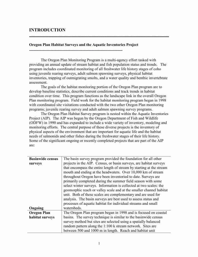
Riparian conifers: total density and density of large riparian conifers Density and size of conifers in the riparian zone are a measure of riparian health in forested coastal basins. Coniferous trees provide shade, stability and large woody debris to the streams.

The density of riparian conifers of all size classes varied by geographic region, with two groups visible on cumulative frequency distribution graphs (Figure 3). The same groupings were present in the 1998-2000 composite dataset. Densities of riparian conifers were higher than reference conditions in the Umpqua and South Coast MA’s. The North Coast, Mid South Coast and Mid Coast regions had fewer conifers within 30

12

m of the stream channel. However, approximately 50% of all streams had streamside vegetation comprised of at least 300 conifer trees per 305m of stream length.

Large riparian conifers were defined as conifers >0.5 m in diameter. At least 35% of sites in each MA did not contain large conifers in three riparian transects surveyed at each site. Nearly 70% of all sites in the Mid-South were lacking large conifers. All regions had lower than reference level quantities of large riparian conifers with the Mid-South having significantly lower levels (Figure 5). Table 6. Cumulative frequency distribution quartiles and summary statistics for riparian conifer metrics. Riparian Quartiles 2000 dataset 98-00 datasets Quartiles Quartiles Analysis Area (n) Mean S.D. 25th 50th 75th (n) Mean S.D. 25th 50th 75thcon >0.5 m dbh/ North Coast 46 35.3 44.6 0 20 61 139 33.9 48.2 0 0 70 305m of stream Mid Coast 40 27.3 37.1 0 20 41 124 34.8 47.2 0 12 60 (large riparian Mid-South Coast 37 13.2 28.1 0 0 20 121 30.1 58.9 0 0 25 conifers) Umpqua 36 49.1 61.8 0 20 61 117 80.1 115.6 0 20 125 South Coast 43 53 69.1 0 30 71 133 59.7 83.2 0 20 90 con >1.0 m dbh/ North Coast 46 5.3 12.4 0 0 0 139 7.3 18.8 0 0 0 305m of stream Mid Coast 40 11.5 17.7 0 0 20 124 8.1 14.5 0 0 12.5(very large Mid-South Coast 37 1.6 7.4 0 0 0 121 8 25.2 0 0 0 riparian con) Umpqua 36 14.7 30.2 0 0 0 117 24 44.6 0 0 20 South Coast 43 25 49.9 0 0 20 133 19.7 39.7 0 0 17 total conifers/ North Coast 46 521 835.6 132 305 660 139 391.7 567.5 100 225 460 305m of stream Mid Coast 40 321.2 388.3 61 203 406 124 336.6 334.5 100 275 460 Mid-South Coast 37 559.3 854.9 81 254 480 121 451 714.6 30 175 450 Umpqua 36 782.4 787.1 142 569 1077 117 875.3 800.6 275 710 1280 South Coast 43 721.6 658.6 158 519 1163 133 765.3 696.4 210 590 1100

0 30 6015 Miles

0 40 8020 Kilometers

0

25

50

75

100

0 20 40 60 80 100

Percent pool habitat

Cum

ulat

ive

perc

ent s

trea

m le

ngth

North Coast (n=46)

Mid Coast (n=40)

Mid-South Coast (n=37)

Umpqua (n=36)

South Coast (n=43)

2000 Reference

Figure 2.1: Cumulative distribution of frequency for the percent gravel in riffle unitsfor western Oregon.

Figure 2.2: Cumulative distribution of frequency for the percent pools for western Oregon.

Legend

Percent pool habitat

<15%

15-30%

30-60%

60-80%

>80%

Percent gravel in riffle units

<15%

15-30%

30-45%

45-60%

>60%

0

25

50

75

100

0 20 40 60 80 100

Percent gravel in riffle units

Cum

ulat

ive

perc

ent s

trea

m le

ngth

North Coast (n=41)

Mid Coast (n=34)

Mid-South Coast (n=31)

Umpqua (n=32)

South Coast (n=31)

2000 Reference

Oregon Plan Survey Sites 2000

Streams (1:500k)

13

Figure 2: Map and cumulative freqeuncy distribution graphs displaying the percent pool habitat and the percent gravel in riffle units.

Figure 2.3: Map of western Oregon displaying the percent pool habitat and the percentgravel in riffle units.

0 25 5012.5 Miles

0 30 6015 Kilometers

0

25

50

75

100

0 20 40 60 80 100

Density of wood volume ( m^3 / 100 m )

Cum

ulat

ive

perc

ent s

trea

m le

ngth

North Coast (n=46)

Mid Coast (n=40)

Mid-South Coast (n=37)

Umpqua (n=36)

South Coast (n=43)

2000 Reference

0

25

50

75

100

0 300 600 900 1200 1500 1800 2100 2400 2700 3000

Density of riparian conifers ( Number / 305 m )

Cum

ulat

ive

perc

ent s

trea

m le

ngth

North Coast (n=46)

Mid Coast (n=40)

Mid-South Coast (n=37)

Umpqua (n=36)

South Coast (n=43)

2000 Reference

Figure 3.1: Cumulative distribution of frequency for the density of woody debris volume in western Oregon.

Figure 3.2: Cumulative distribution of frequency for the density of riparian conifers in western Oregon.

LegendVolume of large woodydebris per 100m

<20

20-30

30-70

70-115

>115

Density of riparian conifers

<300

300-750

750-1500

1500-2800

>2800

Streams (1:500k)

Oregon Plan Survey Sites 2000

14

Figure 3.3: Map of western Oregon displaying the volume of large woody debris/100mand the density of riparian conifers.

Figure 3: Map and cumulative frequency distribution graphs displaying the volume of large woody debris/100m and riparian conifers.

0 30 6015 Miles

0 30 6015 Kilometers

Figure 4.1: Cumulative distribution of frequency for the number of pools >1.0 m deepper km for western Oregon.

Figure 4.2: Cumulative distribution of frequency for the percent fines in riffle units for western Oregon.

0

25

50

75

100

0 2 4 6 8 10

Density of deep pools ( Number / km )

Cum

ulat

ive

perc

ent s

trea

m le

ngth

North Coast (n=46)

Mid Coast (n=40)

Mid-South Coast (n=37)

Umpqua (n=36)

South Coast (n=43)

2000 Reference

0

25

50

75

100

0 20 40 60 80 100

Percent fines in riffle units

Cum

ulat

ive

perc

ent s

trea

m le

ngth

North Coast (n=41)

Mid Coast (n=34)

Mid-South Coast (n=31)

Umpqua (n=32)

South Coast (n=31)

2000 Reference

Legend

Pools > 1.0m per km

1 or less

1-3.5

3.5-5

5-7

> 7

Percent fines in riffle units

<20

20-35%

35-50%

50-70%

>70%

Streams (1:500k)

Oregon Plan Survey Sites 2000

Figure 4: Map and cumulative frequency distribution graphs displaying the percent of pool habitat and percent gravel in riffle units.

15

Figure 4.3: Map of western Oregon displaying the percent of pool habitat and the percent gravel in riffle units.

0 30 6015 Miles

0 30 6015 Kilometers

0

25

50

75

100

0 20 40 60 80 100

Density of wood volume ( m^3 / 100 m )

Cum

ulat

ive

perc

ent s

trea

m le

ngth

North Coast (n=46)

Mid Coast (n=40)

Mid-South Coast (n=37)

Umpqua (n=36)

South Coast (n=43)

2000 Reference

Figure 5.1:Cumulative distribution of frequency for the density of woody debris volume forwestern Oregon.

Figure 5.2: Cumulative distribution of frequency for density of large riparian conifers (>0.5m dbh) per 1000ft for western Oregon.

0

25

50

75

100

0 50 100 150 200 250 300 350 400

Density of large riparian conifers ( Number / 305 m )

Cum

ulat

ive

perc

ent s

trea

m le

ngth

North Coast (n=46)Mid Coast (n=40)Mid-South Coast (n=37)Umpqua (n=36)South Coast (n=43)2000 Reference

Oregon Plan Survey Sites 2000

Figure 5.3: Map of western Oregon displaying the volume of large woody debris/100mand the density of large riparian conifers (>0.5m dbh).

Figure 5: Map and cumulative frequency distribution graphs displaying the density of woody debris volume and large riparian conifers.

LegendVolume of large woodydebris/100m

Density of large riparian conifers (>0.5m dbh)

Streams (1:500k)

<10

10-50

50-100

100-150

>150

16

< 10

10-20

20-30

30-50

>50

17

Fish Surveys

Fish presence/absence surveys using electofishing were conducted at habitat sites

outside of known coho salmon distribution in all Mas to assess distributions of all salmonid species. A total of 101 sites were sampled in 2000 with fish found at 72 sites. Of the 72 sites that contained fish, nine were found with coho salmon. One of the nine sites was determined to be within the currently defined range of coho. The other eight contributed to an expansion of the distribution of coho by 6.72 kilometers (Figure 6).

The summary statistics for these sites describe areas whose geomorphology more closely resemble sites outside the range of coho. The amount of secondary channel area, gradient, valley width, wetted width and active channel width and height (Table 7) are all similar to the statistics defined for areas outside the range of coho (Table 2). However, stream gradient was high (4.4%), but the percent of pools and amount of wood was adequate for juvenile coho salmon. While these eight sites describe areas with marginal habitat for coho it is important to consider the full range of coho habitat needs and potential distributions.

Table 7. Summary statistics for sites surveyed outside the range of coho but where coho salmon were sampled.

Watershed Area (km2)

Secondary Channel

Area (% of Total)

Gradient (%)

Valley Width Index

Wetted Width

(m)

Active Channel Width

(m)

Active Channel Height

(m) Mean 6.9 4.6 4.4 3.3 3.2 7.5 0.5

Median 4.1 3.0 4.4 2.6 3.3 7.9 0.5 Number of

Pools Percent Pools

% Gravel in Riffles

% Fines in Riffles

Pieces of Wood

Wood Volume

Number of Jams

Mean 13.9 31.1 35.2 16.8 13.3 30.4 2.8 Median 14.0 34.2 28.0 17.5 14.0 15.6 3.0

Figure 6. Map of sites in 2000 where coho were found outside their expected distribution.

18

Habitat Condition and Quality 98-00 The Oregon Plan’s robust sampling design provides flexibility in statistical

analysis. To determine overall habitat condition and quality for the entire 1998-2000 time period we combined the sites from all years into one dataset. Summary statistics and quartile calculations showed results that were generally similar to the annual summaries (Tables 3-6). To compare between years we also displayed the data lumped by year in box plots (Figure 7).

A comparison of the 50th percentile mark (median value) showed one variable in the overall dataset that did not follow the 2000 results. Compared to the annual summaries, the percent of fines in riffle units on the North Coast appeared to be lower in the 2000 field season while fines on the South Coast were higher in 2000.

The box plot display supports the consistency between years that is visible in an assessment of quartiles (Figure 7). There is some variability around the mean variables and a few outliers visible but the overall pattern between years is similar. Sites in the 1998-2000 dataset were also assessed based on habitat quality and spatial distribution. The sites were compared to six benchmark criteria developed by the census survey program with the total number of benchmarks exceeded tallied for each site. We divided the sites based on their location within and outside the distribution of coho.

North Coast, Mid South and South Coast Monitoring Areas showed little difference in habitat quality based on coho distribution (Table 8). The Mid-Coast appeared to have higher scoring sites inside the range of coho while sites in the Umpqua MA tended to score higher outside the range of coho.

The Mid-South monitoring area had the highest percent of sites with good habitat quality both inside and outside the range of coho. The Umpqua had the lowest percent of high quality sites inside the range of coho (Table 8).

Sites that exceeded 5 benchmark conditions were rare. Two were found in the Umpqua, two in the Mid-South and one in the South Coast Monitoring area. Four of these sites were outside the range of coho (Figures 8 and 9). No sites were found that exceeded all 6 benchmark conditions used for comparison. In addition, approximately 25% of the sites met none or one benchmark.

Table 8. Benchmark summary table Percent of sites that met 3 or more benchmark criteria

Inside the range of coho (%)

Outside the range of coho (%)

North Coast 19 21 Mid-Coast 37 28 Mid-South 44 45 Umpqua 17 26 South Coast 26 25

19

1998 1999 2000Y EAR

0

20

40

60

80

100

PC

TPO

OL

1998 1999 2000Y EAR

0

20

40

60

80

100

RIF

GR

AV

1998 1999 2000YEAR

0

20

40

60

80

100

RIS

ND

OR

1998 1999 2000Y EAR

0

10

20

30

PL1

PKM

1998 1999 2000Y EAR

0

100

200

300

400

500

600

CO

N20

PLS

1998 1999 2000Y EAR

0

100

200

300

CO

N36

PLS

Figure 7. Box plots displaying composite data for variables collected by year.

1998 1999 2000YEAR

0

1000

2000

3000

4000

5000

TCO

N

1998 1999 2000YEAR

0

50

100

150

200

250

LWD

VO

L1

1998 1999 2000YEAR

0

40

80

120

160

LWD

PIE

C1

1998 1999 2000YEAR

0

10

20

30

40

JAM

S.K

M

1998 1999 2000YEAR

0

4

8

12

KE

YLW

D1

Figure 7. (continued)

Axis Legend: PCTPOOL = percent pool habitat RIFGRAV = percent gravel in riffle units RIFSNDOR = percent sand and organics in riffle units PL1PKM = number of pools > 1.0 m deep per km CON20PLS = number of conifers > 20in dbh CON36PLS = number of conifers > 36in dbh TCON = total riparian conifers LWDVOL1 = volume of large woody debris per km LWDPIEC1 = number of pieces of large woody debris/km JAMS.KM = number of wood jams per km KEYLWD1 = number of key pieces of wood (>0.5mdbh and 6m long) per km

20

21

Trends 1998-2000

The summary statistics for 1998, 1999 and 2000 were similar for all variables (Tables 3-6). The cumulative frequency distribution curves displayed some variation with the density of large riparian conifers in the 1999 dataset showing the greatest difference (Figure 8). While we would not expect to detect a significant change or trend in overall habitat condition is such a short time, the consistent data signal from information collected across western Oregon points to other considerations (Appendix 2). The question has become what is causing the consistency, and likewise, what would register a change.

The similarity between years in data collected supports the spatially random sample design as one that consistently characterizes patterns across the landscape. The rigor of the sampling design allows for the detection of trend, the limiting factor was years of sampled data.

The only statistically significant difference between years was detected in the cumulative distribution of frequency (CDF) curves for large riparian conifers. The 1999 survey season was significantly different from 1998 and 2000 (p-value <0.05) with more

sites in 1999 having large riparian conifers than in other years. It is important to observe that the shape of the curves were the same with 1999 appearing to be offset. This indicates concordant variation in which the entire dataset is different as opposed to differences that are associated with site specific annual variation (Larsen et al, 2001, Kincaid, T.M. 2000). For a

variable like large riparian conifers, an annual effect was not to be expected since densities and growth of large conifers in most of western Oregon was stable (large riparian conifers on fish bearing streams are generally protected under Department of Forestry timber harvest regulations and annual growth rates were not detectable with our survey methods). Therefore, the spatially random sample pull for 1999 focused on a slightly different population of streams than in 1998 and 2000 and included higher numbers of streams in unmanaged areas or headwater streams where large riparian conifers are more common.

0

25

50

75

100

0 50 100 150 200 250 300 350 400

Density of large riparian conifers ( Number / 305 m )

Cum

ulat

ive

perc

ent s

tream

leng

th

2000

1999

1998

2000 Reference

Figure 8. Cumulative distribution of frequency curves showing large riparian conifers for 1998, 1999 and 2000 field season.

22

Detecting a significantly different density for large riparian conifers was useful in determining the overall effectiveness of the sample pull. This habitat metric is sensitive to survey collection and represents a feature that was rare compared to other sizes and types of trees. While a statistically significant difference in the density of large riparian conifers was detected in the sample set other habitat characteristics did not change significantly.

More research is necessary to determine the level of correlation of variables at the site level. For example, the significant difference detected in large riparian conifers did not follow discernable changes in another variable. This may be the result of actual field conditions, or may point to limitations in the ability of our sampling design to detect environmentally significant changes or relationships at the site level. That is, large trees may affect condition downstream of the site, or landscape conditions above the site may influence instream conditions.

In determining changes in habitat and temporal trends, climatic cycles and other landscape level patterns are important considerations. Mild winter weather conditions and low rainfall between 1998 and 2000 contribute to the consistency that was found between years. It will be interesting to determine if changes are discernable as winter climatic conditions vary in coming years.

Another facet of the environment that is pertinent to the discussion of trends is land use. Land use has altered the face of western Oregon. While the Oregon Plan Monitoring program was not designed to detect or measure changes based on historic comparisons, the lack of variability among regions and between years contributes to a hypothesis that broad scale changes have occurred and continue to influence the character of streams in coastal basins.

0 30 6015 Miles

0 50 10025 Kilometers

Benchmarks are measurements of habitat attributes that are associated with poor or fair habitat for salmonids. In order to guage habitat condition 6 benchmarks that denote good salmon habitat were identified. The number of benchmarks that were met at a site were tallied and are represented on the map. The benchmark thresholds that were considered are: >35% pool area Volume of large woody debris >20/100m <12% fines in riffles >70% shade >=35% gravel in riffles riparian conifers >150 /305m

Oregon Plan Survey Sites Inside the Range of Coho 1998-2000

Benchmark values tallied per site

North Coast GCG 1998-2000: Inside the distribution of coho (n=75)

11%

29%

41%

15%4%

0

1

2

3

4

Mid-Coast GCG 1998-2000: Inside the distribution of coho (n=70)

4%

23%

36%

33%

4%

0

1

2

3

4

Umpqua GCG 1998-2000: Inside the distribution of coho (n=41)

12%

34%

37%

10%7%

0

1

2

3

4

Mid-South Coast GCG 1998-2000: Inside the distribution of coho (n=34)

9%

12%

35%

26%

15%3%

0

1

2

3

4

5

South Coast GCG 1998-2000: Inside the distribution of coho (n=8)

13%

24%

37%

13%

13%

0

1

2

3

4

24

Figure 10: Map of sites for 1998-2000 showing sites that exceeded a variety of ODFW's benchmark criteria. Sites displayed are located inside the expected distribution of coho.

Legend

Streams (1:500k)

Benchmark Totals0

1

2

3

4

5

0 30 6015 Miles

0 50 10025 Kilometers

Benchmarks are measurements of habitat attributes that are associated with poor or fair habitat for salmonids. In order to guage habitat condition 6 benchmarks that denote good salmon habitat were identified. The number of benchmarks that were met at a site were tallied and are represented on the map. The benchmark thresholds that were considered are: >35% pool area Volume of large woody debris >20/100m <12% fines in riffles >70% shade >=35% gravel in riffles riparian conifers >150 /305m

Oregon Plan Survey Sites Outside the Range of Coho 1998-2000

Benchmark values tallied per site

North Coast GCG 1998-2000: Outside the distribution of coho (n=47)

32%

45%

17%

4% 2%

0

1

2

3

4

Mid-Coast GCG 1998-2000: Outside the distribution of coho (n=39)

5%8%

59%

23%

5%

0

1

2

3

4

Mid-South Coast GCG 1998-2000: Outside the distribution of coho (n=56)

21%

30%

27%

16%2% 4%

0

1

2

3

4

5

Umpqua GCG 1998-2000: Outside the distribution of coho (n=60)

32%

39%

17%

2% 3%7%0

1

2

3

4

5

South Coast GCG 1998-2000: Outside the distribution of coho (n=65)

29%

38%

20%

5% 2% 6%0

1

2

3

4

5

23

Figure 9: Map of sites for 1998-2000 showing sites that exceeded a variety of ODFW's benchmark criteria. Sites displayed are located outside the expected distribution of coho.

Legend

Streams (1:500K)

Benchmark Totals0

1

2

3

4

5

25

Resurvey Analysis

An assessment of variable precision incorporated annual and composite variability for 1998-2000 (Table 9). The complete dataset encompassed 724 habitat survey sites and 85 sites where a repeat survey was conducted. The signal to noise ratio for channel length, gradient, percent dammed pools, deep pools per km, and 0.3 m conifers per 305 m of stream length varied widely between years, while the precision (reported as the standard deviation and coefficient of variation) remained consistently low. Measurements of signal to noise between years were consistent for percent secondary channels, percent fines, percent gravel, percent fines in riffles and percent gravel in riffles. Signal to noise ratios for woody debris were low but precision remained high. As in previous years, it appeared that a few sites with large amounts of wood proved difficult to count consistently thereby reducing the overall accuracy of the wood data collected. Resurvey analysis also indicated low signal to noise ratios for large riparian conifers (> 0.5m dbh) (Table9). While there is variability in the counts, the standard deviation remained low (Table 6). As with wood variables, this means that while error in counts is common, the numbers of large riparian conifers are still useful for comparison purposes. All signal to noise ratios for variables in the combined 1998-2000 dataset exceeded a value of 2 with several dependent and independent variables with high ratios. Reliable independent variables included channel length, channel width, floodprone width and gradient. Reliable dependent variables were percent secondary channels, percent pools, percent dammed pools, deep pools per km, percent fines, percent bedrock and percent fines in riffles.

26

Table 9. Signal to Noise Ratios for 2000 and combined 1998-2000

Variables Year S.D. (repeats) CV S:N Variables Year S.D. (repeats) CV S:NIndependent Channel 1998 47.8 6.6 29.8 Dependent % Bedrock 1998 2.9 27.1 21.6 Length 1999 26.7 3.5 93.8 (continued) 1999 2.8 27.9 20.3 2000 23.8 3.4 114.7 2000 4.6 47.8 8.2 1998-2000 34.8 4.8 55.2 1998-2000 3.5 34.4 13.9 Channel 1998 1.3 18.1 13.7 % Riffle Fines 1998 7.6 30.2 7.6 Width 1999 1.7 19.5 29.8 1999 7.6 29.7 8.7 2000 0.6 14.9 39.5 2000 10.2 41.5 5.4 1998-2000 1.6 18.4 27.8 1998-2000 8.6 34.1 6.7 Floodprone 1998 3.7 25.9 10.0 % Riffle 1998 9.5 28.3 3.3 Width 1999 3.4 27.6 11.2 Gravel 1999 10.3 26.2 4.5 2000 3.1 20.9 39.8 2000 16.1 38.9 1.6 1998-2000 4.4 32.0 10.4 1998-2000 11.9 31.6 2.8 Gradient 1998 0.5 8.9 172.9 Wood Pieces 1998 3.6 24.9 13.4 1999 1.8 31.6 11.8 per 100 m 1999 4.2 23.8 2.1 2000 0.8 16.9 47.6 2000 10.2 70.1 2.2 1998-2000 1.1 20.7 30.9 1998-2000 9.4 60.8 2.2Dependent % Secondary 1998 3.0 70.0 4.3 Wood Volume 1998 7.4 34.2 11.0 Channels 1999 3.1 66.2 7.9 per 100 m 1999 9.4 35.7 2.5 2000 3.0 74.8 4.4 2000 17.3 63.9 4.0 1998-2000 2.9 68.9 5.6 1998-2000 15.8 64.3 3.6 % Pools 1998 8.1 30.2 6.8 Key Wood 1998 0.6 70.9 3.8 1999 7.7 23.7 27.3 Pieces/100m 1999 1.5 136.5 1.7 2000 5.8 16.9 18.4 2000 1.0 88.4 3.7 1998-2000 7.1 23.2 17.0 1998-2000 1.1 108.4 2.4 % Dammed 1998 0.9 18.5 235.7 Wood Jams 1998 2.6 52.4 5.3 Pools 1999 5.6 112.2 6.8 per km 1999 1.7 36.6 6.4 2000 2.6 45.7 34.0 2000 3.0 51.1 5.5 1998-2000 3.9 76.6 13.6 1998-2000 1.9 49.7 4.5 Deep Pools / 1998 0.7 28.9 33.4 Shade 1998 5.2 6.7 11.5 km 1999 1.1 54.1 5.8 1999 6.2 7.5 6.2 2000 1.0 43.7 12.7 2000 9.8 12.8 4.1 1998-2000 1.2 51.5 9.3 1998-2000 7.6 9.6 5.5 Residual 1998 0.3 55.7 1.7 20 in. Conifers 1998 20.0 49.5 10.0 pool depth 1999 0.1 13.5 14.4 per 1000 ft 1999 69.4 98.3 2.3 2000 0.1 12.6 13.2 2000 22.0 61.5 5.6 1998-2000 0.2 31.9 3.5 1998-2000 42.4 88.3 3.3 % Fines 1998 6.8 23.6 11.5 36 in. Conifers 1998 6.0 58.0 24.6 1999 7.8 26.2 9.1 per 1000 ft 1999 32.8 161.7 1.6 2000 5.6 18.8 19.3 2000 14.7 125.7 4.0 1998-2000 6.7 22.9 12.4 1998-2000 23.1 168.3 2.1 % Gravel 1998 9.1 36.3 2.0 1999 7.6 27.6 4.1 2000 8.1 27.1 3.8 1998-2000 8.1 30.0 3.2

27

CONCLUSIONS

The first three years of landscape level habitat sampling have allowed for the

collection of baseline conditions that are crucial for trend analysis. Statistically significant changes in landscape features take many years or a large-scale hydrologic event to detect (Jones et al 1996). Along with the ability to detect trends in the future we have also effectively described the current status of Oregon coho habitat. The next step for this project will be to incorporate patterns of juvenile and spawning coho distributions that have been detected by the other Oregon Plan Monitoring Projects.

As would be expected, stream conditions in western Oregon from 1998, 1999 and

2000 are statistically similar. This points to a variety of conditions including mild winters, dry summers, random and spatially balanced sample pulls and the fact that it takes many years for landscape level changes to occur and become detectable. In the future we expect sample sets that include normal and severe seasonal weather patterns. The variability that is detected after these years may help in determining where and what events cause a discernable change.

Signal to Noise analysis is consistently pointing to variables that have high and

low levels of precision and reliability. This analysis is not only useful for Oregon Plan analysis of habitat data but has provided useful insight into the accuracy of Aquatic Inventories Project stream survey data collection and the analysis of comprehensive census survey information. Even though a habitat parameter may have a low signal to noise ratio, it may still be useful to collect and summarize, given appropriate interpretation of its value.

The most significant difference between the 3 years of field data was found in the

1999 riparian conifer counts. This pointed to a condition in the sample pull that may have favored areas where conifer counts were high. This occurred even with the spatially random sampling design.

The high percentage of private landowners affects how many surveys can be

accomplished in lower basin areas. There were more landowner access denials in 2000 than in previous field seasons. The level of denial is great enough that lower basin areas are now not equally represented in the surveyed sample. This bias may be resulting in an assessment of habitat quality that is artificially high (Thom et al. 2001).

28

ACKNOWLEDGEMENTS

The Oregon Plan habitat survey program would not have been successful if not for the participation and cooperation of a wide variety of groups and individuals. The private landowners and large corporate landholders who gave us permission to survey and who often helped guide our field crews when accessing streams were crucial participants in this study. Local ODFW district biologists and watershed councils provided scope and assistance to field crews and in the general coordination of efforts.

Field crew supervision was completed by a group of conscientious and hard working ODFW biologists. Kelly Reis, Peggy Kavanagh, Jen Bock, Charlie Stein, Paul Jacobsen, Trevan Cornwall and Paul Scheerer worked long hours coordinating crews and equipment in the field. Kelly Reis and Lisa Krentz provided expert data organization and analysis assistance. LaNoah Babcock’s contribution to data entry was also appreciated.

29

REFERENCES

Bodenmiller, D., P. Lawson, D. McIsaac, and T. Hickelson. 1997. Fishery Management Regime to Ensure Protection and Rebuilding of Oregon Coastal Natural Coho Incorporation. The Regulatory Impact Review. Initial Regulatory Flexibility Analysis, and Environmental Impact Statement. Amendment 13 to the Pacific Coast Salmon Plan. Pacific Fishery Management Council, Portland, OR. Jones, K.K., S Foster and K.M.S. Moore. 1998. Preliminary Assessment of 1996 Flood Impacts: Channel Morphology and Fish Habitat. Oregon Dept. of Fish and Wildlife. Corvallis Research Lab white paper. Kincaid, T.M. 2000. Testing for differences between cumulative distribution functions from complex environmental sampling surveys. Proceedings of the American Statistical Association Section on Statistics and the Environment, Alexandria, VA: American Statistical Association. pp39-44. Larsen, David P., Thomas M. Kincaid, Steven E. Jacobs, and N. Scott Urquhart. 2001. Designs for Evaluating Local and Regional Scale Trends. BioScience Vol. 51 No. 21 December 2001. pp 1069-1078. Moore, K. M. S., K. K. Jones, and J. M. Dambacher. 1997. Methods for stream habitat surveys. Oregon Dept. of Fish and Wildlife Information Report 97-4. Portland, OR 40p. Nickelson, Thomas E. 2001. Population Assessment: Oregon Coast Coho Salmo ESU. Oregon Department of Fish & Wildlife Information Report 2001-02. Portland, OR pp5-8. Rodgers, J.D. 2000. Abundance of Juvenile Coho Salmon in Oregon Coastal Streams, 1998 and 1999. Monitoring Program Report Number OPSW-ODFW-2000-1, Oregon Department of Fish and Wildlife, Portland.

Stevens, D. L., Jr. 1997. Variable density grid-based sampling designs for continuous spatial populations. Environmetrics. pp 167-195.

Stevens, D. L., Jr. and A. R. Olsen. 1999. Spatially restricted surveys over time for aquatic resources. Journal of Agricultural, Biological, and Environmental Statistics. Thom, Barry A., P. S. Kavanagh and K. K. Jones. 2001. 2000 Reference Site Selection and Survey Results. Monitoring Program Report Number OPSW_ODFW-2001-6, Oregon Department of Fish and Wildlife, Portland, Oregon.

30

Thom, B. A., K. K. Jones, P. S. Kavanagh, K. E. M. Reis. 2000. Stream Habitat Conditions in Western Oregon, 1999. Monitoring Program Report Number OPSW-ODFW-2000-5, Oregon Department of Fish and Wildlife, Portland, Oregon. Thom, B. A., K. K. Jones, and R. L. Flitcroft. 1999. Stream Habitat Conditions in Western Oregon, 1998. Monitoring Program Report 1999-1 to the Oregon Plan for Salmon and Watersheds, Governor’s Natural Resources Office, Salem, Oregon. Thom, Barry et al 2000. 1999 Oregon Plan Monitoring Report. Thom, B. A., K. K. Jones, and C. S. Stein. 1998. An analysis of historic, current, and desired conditions for streams in western Oregon. Section IV-ODFW pages 33-56 In The Oregon Plan for Salmon and Watersheds 1998 Annual Report.

Zar, J. H. 1984. Biostatistical Analysis, 2nd edition. Prentice-Hall, Englewood Cliffs, new Jersey. 718 pp.

31

APPENDICES

Appendix 1: ODFW Benchmarks

Habitat Benchmarks

Kelly M.S. Moore Oregon Department of Fish and Wildlife

1 April 1997

The development of quantitative criteria for habitat quality provides an important tool for evaluation of current habitat condition and for setting goals for improved habitat values. Benchmark values, derived from reference conditions, analysis of variable distribution, and compiled from published values, provide the initial context for evaluating measures of habitat quality. Comparison of habitat measures to benchmark values, however, must be made with caution, taking into consideration both the geomorphic template that defines the potential of the system and the combination of natural disturbance and management history that influence the expression of that potential. The ecological potential of each stream should be considered when comparing values to the benchmarks. The ecological potential for performance will vary depending on the ecoregion, geology, natural disturbance history, local geomorphic constraints on habitat, and the size and location of the stream within its watershed. When interpreting stream habitat data in the context of these benchmarks, it is important to recognize that the capacity of a stream reach meet benchmark values is a function of both its ecological setting and the patterns of land use and management that modify “performance” of the stream relative to benchmark values. Conceptually, it would appear valuable to further develop benchmark values specifically targeted to streams within individual strata of ecoregion, geologic, disturbance, etc. However, our experience with analysis of stream data from over 5,000 miles of surveys located in all regions of Oregon has led away from this approach. We have found that as the strata for interpretation becomes more limiting, each stream or small group of streams needs to be interpreted in terms of their individual characteristics and land use history as compared to general performance values. It also becomes more useful to look at combinations and interactions of features rather than single out individual values. At this level, each stream is essentially unique. In addition, as attempts to “fine tune” benchmark values focus on smaller geographic areas and sample sizes, the limited availability of reference sites and insufficient information on the range of natural conditions within the sample make such an attempt at precise development of benchmarks impractical and a misapplication of the approach.

32

Benchmark values are best applied to the evaluation of conditions in individual streams or stream reaches. The benchmarks provide a context for interpretation and as a starting point for more detailed and meaningful analysis. For each habitat variable that meets or fails to meet desirable habitat benchmarks, the investigation and analysis should focus on both proximal and historic causes. An important part of this work is to interpret channel and riparian conditions in a broader landscape context. Benchmark values are also very useful at looking as overall conditions within a watershed, basin, or region. Whenever aggregating reach information to this level, however, it must be remembered that under natural condition some percentage of a watershed, basin, or region may always be classified as below desirable condition. Land use and management activities will modify this percentage, commonly increasing the amount of habitat demonstrating undesirable conditions. The impact of current land use and management designed to improve these conditions is difficult to assess against the background of natural disturbance and past management and use. At the basin and region level in particular, the analysis required to evaluate these relationships has not been done. Given these qualifications, the use of the ODFW Habitat Benchmarks requires the application of common sense and openness to further analysis. Proper use can reveal important trends in habitat condition and suggest appropriate management action. Development of Benchmark Values: The Habitat Benchmark values for desirable (good) and undesirable (poor) conditions are derived from a variety of sources. Habitat characteristics representative of conditions in stream reaches with high productive capacity for salmonid species are used as a starting point. Values from “reference” reaches were used to develop standards for large woody debris and riparian conditions. These reference values were then compared to the overall distribution of values for each habitat characteristic expressed as a frequency distribution within a basin or region. From this analysis, it was generally apparent that values from the 66th or higher percentile could represent desirable or good conditions and values from the 33rd or lower percentile represent desirable or poor conditions. This development of benchmarks from the frequency distributions was made specific to appropriate stream gradient, regional, and geologic groupings of the reach data. Finally, values for habitat characteristics such as pool frequency, silt-sand-organics, and shade were developed from a comparison between the distributions and generally accepted or published values. Benchmark Values and Example Distributions: The Habitat Benchmark values developed for use for evaluating Oregon streams and watersheds are summarized in Table 1. Where appropriate, the values have been adapted for application to large or small stream reaches with high or low gradient. Values for fine sediments in riffles reflect differences in parent material and channel gradient. Stream shading refers to the percent of the total horizon shaded by topography and vegetation and are adjusted for stream width and geographic region. Large woody debris and

33

riparian conifer values apply only to reaches within forested basins. A summary analysis of habitat values relative to the benchmarks is shown in Table 2 and Figure 1. Note: This information excerpted from Moore, K. M. S. and K. K. Jones (in prep.) Analysis and application of stream survey data for restoration planning and quantification of change at the watershed scale. ODFW Research Section. Corvallis, OR Draft 12/96. Table 1: ODFW Aquatic Inventory and Analysis Projects: Stream Channel and Riparian

Habitat Benchmarks

POOLS UNDESIRABLE DESIRABLE POOL AREA (% Total Stream Area) <10 >35 POOL FREQUENCY (Channel Widths Between Pools) >20 5-8 RESIDUAL POOL DEPTH SMALL STREAMS(<7m width) <0.2 >0.5 MEDIUM STREAMS(≥ 7m and < 15m width) LOW GRADIENT (slope <3%) <0.3 >0.6 HIGH GRADIENT (slope >3%) <0.5 >1.0 LARGE STREAMS (≥15m width) <0.8 >1.5 COMPLEX POOLS (Pools w/ wood complexity >3/km) <1.0 >2.5 RIFFLES WIDTH / DEPTH RATIO (Active Channel Based) EAST SIDE >30 <10 WEST SIDE >30 <15 GRAVEL (% AREA) <15 ≥35 SILT-SAND-ORGANICS (% AREA) VOLCANIC PARENT MATERIAL >15 <8 SEDIMENTARY PARENT MATERIAL >20 <10 CHANNEL GRADIENT <1.5% >25 <12 SHADE (Reach Average, Percent) STREAM WIDTH <12 meters WEST SIDE <60 >70 NORTHEAST <50 >60 CENTRAL - SOUTHEAST <40 >50 STREAM WIDTH >12 meters WEST SIDE <50 >60 NORTHEAST <40 >50 CENTRAL - SOUTHEAST <30 >40

LARGE WOODY DEBRIS* (15cm x 3m minimum piece size) PIECES / 100 m STREAM LENGTH <10 >20 VOLUME / 100 m STREAM LENGTH <20 >30 “KEY” PIECES (>60cm dia. & ≥10m long)/100m <1 >3

34

RIPARIAN CONIFERS (30m FROM BOTH SIDES CHANNEL) NUMBER >20in dbh/ 1000ft STREAM LENGTH <150 >300 NUMBER >35in dbh/ 1000ft STREAM LENGTH <75 >200 * Values for Streams in Forested Basins

35

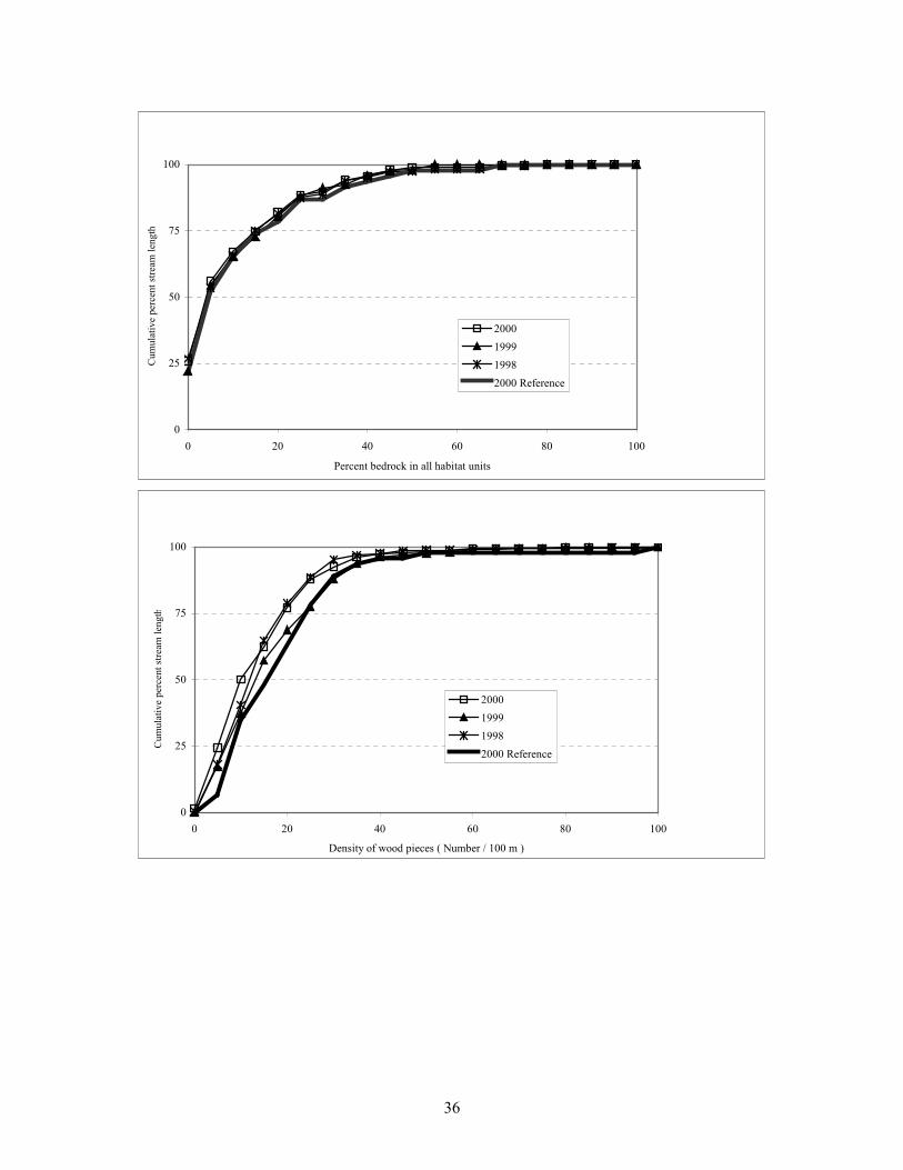
Appendix 2: Cumulative distributions of frequency for 1998, 1999 and 2000

0

25

50

75

100

0 20 40 60 80 100

Percent fines in riffle units

Cum

ulat

ive

perc

ent s

tream

leng

th

2000

1999

1998

2000 Reference

0

25

50

75

100

0 20 40 60 80 100

Percent gravel in riffle units

Cum

ulat

ive

perc

ent s

tream

leng

th

2000

1999

1998

2000 Reference

36

0

25

50

75

100

0 20 40 60 80 100

Percent bedrock in all habitat units

Cum

ulat

ive

perc

ent s

tream

leng

th

2000199919982000 Reference

0

25

50

75

100

0 20 40 60 80 100

Density of wood pieces ( Number / 100 m )

Cum

ulat

ive

perc

ent s

tream

leng

th

2000199919982000 Reference

37

0

25

50

75

100

0 20 40 60 80 100

Density of wood volume ( m^3 / 100 m )

Cum

ulat

ive

perc

ent s

tream

leng

th

2000199919982000 Reference

0

25

50

75

100

0 2 4 6 8 10 12 14 16 18 20

Density of wood jams ( Number / km )

Cum

ulat

ive

perc

ent s

tream

leng

th

2000199919982000 Reference

38

0

25

50

75

100

0 2 4 6 8 10

Density of key wood pieces ( Number / 100 m )

Cum

ulat

ive

perc

ent s

tream

leng

th

2000199919982000 Reference

0

25

50

75

100

0 20 40 60 80 100

Percent pool habitat

Cum

ulat

ive

perc

ent s

tream

leng

th

2000199919982000 Reference

39

0

25

50

75

100

0 2 4 6 8 10

Density of deep pools ( Number / km )

Cum

ulat

ive

perc

ent s

tream

leng

th

2000199919982000 Reference

0

25

50

75

100

0 20 40 60 80 100

Percent channel shading

Cum

ulat

ive

perc

ent s

tream

leng

th

2000199919982000 Reference

40

0

25

50

75

100

0 50 100 150 200 250 300 350 400

Density of large riparian conifers ( Number / 305 m )

Cum

ulat

ive

perc

ent s

tream

leng

th

2000199919982000 Reference

0

25

50

75

100

0 50 100 150 200 250

Density of v ery large riparian conif ers ( Number / 305 m )

Cum

ulat

ive

perc

ent s

tream

leng

th

2000

1999

1998

2000 Ref erence

41

0

25

50

75

100

0 300 600 900 1200 1500 1800 2100 2400 2700 3000Density of riparian conifers ( Number / 305 m )

Cum

ulat

ive

perc

ent s

tream

leng

th

2000199919982000 Reference