developing large woody debris budgets for texas rivers
TRANSCRIPT

Developing Large Woody Debris Budgets for Texas Rivers
by Matthew W. McBroom, Ph.D., CF
Presented to The Texas Water Development Board
In Fulfillment of TWDB Contract No 06
On August 31,2010
LS :21 Wd 0 I ~JnV OlOl
TABLE OF CONTENTS
INTRODUCTION .............................................................................................................. 1 TASK 1 – LITERATURE REVIEW.................................................................................. 2
Biological Significance................................................................................................... 2 Effects on Hydraulics...................................................................................................... 5 Large Woody Debris Input ............................................................................................. 9 Mass Wasting................................................................................................................ 14 LWD Decay .................................................................................................................. 16 Surrounding Forest........................................................................................................ 16 LWD Loading ............................................................................................................... 19 Alphanumeric Classification of LWD .......................................................................... 21 Summary ....................................................................................................................... 23
TASK 2 – CONCEPTUAL MODEL OF LWD DYNAMICS......................................... 24 TASKS 3 AND 4 – LWD MEASURING TECHNIQUES .............................................. 26
Study Site ...................................................................................................................... 26 Field Methods ............................................................................................................... 37 Bankside Vegetation ..................................................................................................... 42 Sample Analysis............................................................................................................ 43
TASK 5 – DECAY ANALYSIS....................................................................................... 45 TASK 6 – STATISTICAL ANALYSIS........................................................................... 47 TASK 7 – LWD STORAGE............................................................................................. 51 TASK 8 – LWD TRANSPORTATION ........................................................................... 55 TASK 9 – LWD DOMINANT DISCHARGE ................................................................. 58 TASK 10 – REPORT OF RESEARCH FINDINGS ........................................................ 61
LWD Mass and Volume ............................................................................................... 61 Woody Debris Dynamics.............................................................................................. 63 Statistical Tests Results................................................................................................. 69 LWD Recruitment Rates............................................................................................... 74 Observed Data and Conceptual Models of LWD Dynamics ........................................ 75 Comparison to Other River Systems............................................................................. 79 Bankside Vegetation Inventory..................................................................................... 81
LITERATURE CITED ..................................................................................................... 85 APPENDIX A – DATA AND STATISTICAL ANALYSIS........................................... 92

Developing Large Woody Debris Budgets for Texas Rivers
Matthew W. McBroom, Ph.D., CF
INTRODUCTION Large woody debris (LWD) has been shown to be an extremely important
structural and functional component for aquatic ecosystems in the lower coastal plain of
the Southeast (Wallace et al., 1993). Benke et al. (1984) found that while LWD habitat
may only be a small part of the total habitat surface in these types of rivers (~4%), it may
support over 60% of the total invertebrate biomass for a river stretch. In addition, these
researchers found that fish species obtained at least 60% of their prey biomass from snag
habitat. Consequently, management practices that alter LWD dynamics may have
dramatic effects on aquatic ecosystem productivity.
While the importance of LWD to ecosystem structure and function in the
Southeast is widely accepted, very little empirical information exists on actually
quantifying LWD biomass and dynamics in the Southeast (including Texas). A great
deal of work has been done in the Pacific Northwest, particularly as related to endangered
and threatened salmonids. Lacking such statutory motivation, fewer resources have been
allocated to the Southeast. However, rapid population growth in recent years coupled
with greater demands on limited water resources has generated concern about the health
and viability of Southeastern river systems. This necessitates developing a LWD budget
for Southeastern rivers to quantify possible management effects on LWD dynamics.
Furthermore, little work has been conducted on developing woody debris budgets where
inputs, outputs, and transformations are quantified over various instream flow regimes.

2
Owing to the critical nature of woody debris for aquatic ecosystems, it is imperative that
woody debris budgets be evaluated in order to ensure that healthy populations of aquatic
life are maintained in Texas rivers.
This report summarizes results from Texas Water Development Board Contract
0604830632. For a complete description of proposed project methodology, see the Scope
of Work (SOW) for this contract. This report is organized according the 10 tasks
outlined in that SOW.
TASK 1 – LITERATURE REVIEW Task Description – Examine the scope of scientific literature that exists on LWD measurement, analysis, modeling, and decay. This first task will be important for determining specific areas where gaps currently exist in the state of the knowledge in LWD, specifically as related to Southeastern Coastal Plain streams. From: Ringer, M.S. May 2009, Characterizing large woody debris dynamics in the lower Sabine River, Texas. M.S. Thesis, Stephen F. Austin State University, 149 pp. Compiled by Matthew McBroom, Ph.D., Michael Ringer, M.S., and Luke Sanders, M.S.
LITERATURE REVIEW
Biological Significance Large woody debris is important to many biological factors and to overall forest
health, especially within sensitive riparian zones (McClure et al., 2004). Ecologically,
LWD provides many important aspects for stream systems. It provides a reservoir for
nutrients and energy vital to the detrital food chain, nutrient cycling, plant growth, and
productivity (Harmon et al., 1986; Muller and Liu, 1991; Huston, 1993; Goodburn and
Lorimer, 1998). Stable debris can slow down the transport of fine organic matter
allowing greater opportunity for biological processing of fine organic detritus (Swanson
et al., 1976). Invertebrates and aquatic insects utilize LWD for egg deposition, a direct

3
and indirect food source, attachment sites for feeding and retreat or concealment, material
for larval cases, and a substratum for pupation and emergent sites (Wallace et al., 1993).
In the northwest, numerous studies have documented the biological, hydraulic and
structural importance of LWD in high gradient, lower order headwater streams (Marzolf,
1978; Bilby and Likens, 1980). In these high gradient streams, LWD plays a minor role
in providing habitat formation in the main channel as the stream order increases (Keller
and Swanson, 1979), with a reduction of LWD with increasing stream orders (Minshall
et. al., 1983). In the low gradient (0.01 – 0.02%) streams throughout the lower Gulf
Coastal Plain however, LWD appears to play a major role in habitat formation in high
order streams (Cudney and Wallace, 1980; Benke et al., 1984). Thorp et al. (1985)
reported rapid colonization of woody substrates introduced into tributaries of the
Savannah River, with most species reaching steady states within one week. Filter feeders
are drawn to LWD as a stable substrate, while gathering invertebrates are attracted to the
epixylic biofilms, which develop in stream woody debris as a food source (Couch and
Meyer, 1992). The colonization of filterers and gatherers becomes a food source for
invertebrate predators, which in turn provide a food source for vertebrate predators.
Along the Satilla River (mean Q: 87 m3/s, gradient: <.0001) sandy substrate along the
main channel, muddy substrate of backwaters and submerged LWD along the outer banks
comprise the main invertebrate habitat. LWD contributed only 4% of the available
habitat, but contained 60% of the total invertebrate biomass and 16% of production.
LWD supported greater taxonomic diversity with 63 invertebrate taxa residing on wood,
compared to only 31 taxa in sandy substrate that encompassed 85% of the available
habitat and 41 taxa in muddy substrate that encompassed 9% of available habitat.

4
Furthermore, 78% of drifting invertebrate biomass originated from LWD and comprised
at least 60% of prey consumed by four of eight major fish species sampled (Benke et al.,
1984). Benke and Wallace (1990) found the wood biomass of 6.5 kg/m2 in the sixth
order Ogeechee River (mean Q: 67.7 m3/s, gradient: < 0.0002), and 5.0 kg/m2 in the
fourth order Black Creek (mean Q: < 45 m3/s, gradient: < 0.003) was similar to first and
second order streams in other regions, but was consistently lower than streams in the
Northwest. The in-channel debris surface of the Ogeechee River and Black Creek was
0.249-0.433 m2/m and 0.191-0.379 m2/m, respectively, depending on the stream stage.
These areas provide sites of high invertebrate diversity with an invertebrate density of 6.6
g dry mass/m2 of debris surface, which results in at least 1.82 g of invertebrate
biomass/m2 of channel bottom (Benke and Wallace, 1990). Similar to other southeastern
studies, Benke and Wallace (1990) found that LWD is preferentially located towards the
outer bank, where outer bank erosion is believed to deliver most of the woody debris to
the channel (Keller and Swanson, 1979). In the Ogeechee River and Black Creek LWD
provides a fairly stable habitat compared to the fine grain sandy substrate typical of
streams in the lower Gulf Coastal Plain. In contrast, the sixth-order reach of the Little
Tennessee River, other sources of stable substrate were available along with LWD, such
as the dense growth of the aquatic macrophyte, Podostemum ceratophyllum covering the
cobble substratum of the river. Here, invertebrate abundance and biomass were
significantly greater on the Podostemum than on LWD (Smock et al., 1992).
The biological role of LWD varies in accordance to the manner in which it affects
stream processes. Invertebrate communities can vary greatly depending on stream size,
depth, cross-sectional area, discharge, gradient and the availability of inorganic substrate.
5
In smaller, high gradient low order streams, LWD more drastically changes the physical
stream structure, which causes the invertebrate community to adapt to food resource
availability and physical environmental factors. LWD can enhance a stream’s ability to
process and conserve nutrient and energy inputs by offering habitats to filtering collectors
who utilize suspended organic particles provided by the current, and are the major
invertebrate functioning group found inhabiting in-stream debris. For example, in high
gradient Appalachian streams at Coweeta, North Carolina, channel depth and width
increase and velocity decreases upstream of added LWD jams, which results in increased
heterogeneity of the stream channel substrate composition as sand, silt and organic matter
is deposited over cobbles and riffles. The increase sedimentation from decreased velocity
at Coweeta resulted in a significant decrease in filtering and scraping invertebrates and an
increase in gatherer invertebrates and trichopteran and dipteran shredders, along with an
increase in predators at the LWD sites relative to cobble and riffle areas (Huryn and
Wallace, 1987). In contrast, low gradient, small coastal plain headwater streams showed
an increase in all functional invertebrate groups, with the exception of gatherers in
response to LWD jams (Smock et al., 1989). The debris jams provided the only stable
habitat in this sandy bottom stream. Dolloff (1993) found that when LWD was removed,
the result would be a loss of pool habitat, lower number and size of fish, and a loss of
biomass in both warmwater and coldwater fish.
Effects on Hydraulics LWD, including trees, snags, and logjams, have been shown to influence stream
morphology (Shields and Nunnally, 1984; Mutz, 2000; MacDonald et al. 1982).
6
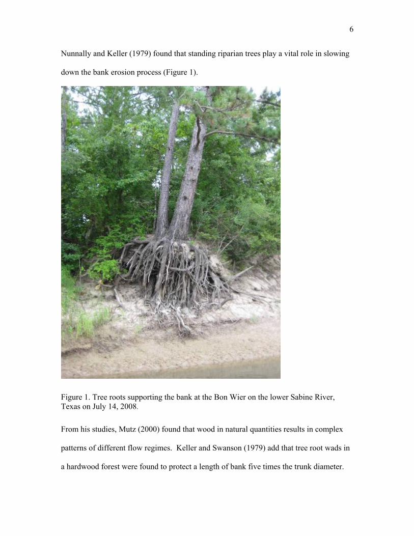
Nunnally and Keller (1979) found that standing riparian trees play a vital role in slowing
down the bank erosion process (Figure 1).
Figure 1. Tree roots supporting the bank at the Bon Wier on the lower Sabine River,
in
Texas on July 14, 2008.
From his studies, Mutz (2000) found that wood in natural quantities results in complex
patterns of different flow regimes. Keller and Swanson (1979) add that tree root wads
a hardwood forest were found to protect a length of bank five times the trunk diameter.

7
The hy
nd
an
s
us
79;
n of
). These combined
ay aff cha
This change in hydraulic conditions exerted by LWD is dependent on the local
el, 1995). The channel shear stress (To) is a function of the density
portioned between various components that each have a particular roughness element
draulics of stream river systems is in a perpetual state of dynamic fluctuation as
the flow of energy is distributed through the drainage basin, shaping the channel
morphology. Removing debris from streams increases current velocity next to banks a
reduces the amount of materials that can provide protection to the bank. This causes
acceleration of bank erosion and a wider channel (Nunnally, 1978). Also, woody debris
helps control river gradient. Abbe et al. (2003) reported that clearing wood from the Red
River in Louisiana caused portions of the river to incise more than 4 m. LWD provide
additional roughness and resistance (Shields and Gippel, 1995) as it redirects the flow of
water, slowing velocity, increasing depth, creating backwaters, local scour and vario
types of pools (Robison and Beschta, 1990). The number of morphological structures
such as bars are also increased because of the presence of LWD (Keller and Tally, 19
Harmon et al., 1986). Because of the additional flow resistance created by the additio
LWD in the stream system, there can be a net increase in sediment storage, changes in
bed texture, and changes in sediment transport (Smith et al., 1993
factors have the ability to change the local and reach-average hydraulic conditions, which
m ect nnel bank stability (Bilby, 1984; Trimble, 1997).
hydraulic conditions, geometry and orientation of LWD, density and spacing of LWD
and its relative size to the flow depth (Shields and Gippel, 1995). Beven et al. (1979)
found that when debris is large in relation to flow depth, the roughness coefficient is
abnormally high (Gipp
of water (ρ), gravity (g), hydraulic radius (R) and the slope of energy gradient (s). To is

8
(Einstein and Banks, 1950), including total grain stress available for sediment transport
(TGS), bed form stress (TBF) and stress due to LWD (TLWD). As the density of debr
increases, To increases in response to the increased water depth. TLWD increases mor
rapidly, so there is a net decrease in TGS as debris is added to the stream (Manga and
Kirchner, 2000). In this study the effect of TBF was ignored because of the stable and
uniform nature of the channel, but in other systems that have irregular bed form,
provide a substantial fraction of the flow resistance (Hey, 1988).
The force (F) per unit area of a piece of LWD immersed in a uniform flow with ve
F
is
e
TBF can
locity V will be:
= ½ ρ CD V2, (1)
coefficient of LWD. This drag coefficient depends on the Reynolds number, Froude
Gippel (1995) found that CD is also dependent on the blockage ration (β), defined as the
diameter of debris and h = mean water depth). The blockage affect from LWD will alter
(Gippel et al., 1992):
CDc / (1- β)2 = CD, (2)
Magna and Kirchner (2000), on the Cultus River in Oregon, used field measurement
calculate the relative contribution of LWD to the reach-average total stress. Th
A
where A is the cross-sectional area of LWD perpendicular to flow and CD is the drag
number, and the shape and orientation of LWD (Magna and Kirchner, 2000). Shields and
ratio of the obstruction area to cross-sectional flow area (β = H/h ; where H = mean
its drag coefficient (CD) from that of a cylinder in a flume (CDc) by a relationship of
s to
e
hydrogeomorphic properties of the Cultus River make it behave like a large natural
lume. The Cultus is spring fed with a near constant discharge (Q) with a steady uniform
flow, has a stable gravel bed, rectangular channel cross section, and a large width to
depth ratio which simplified the analysis because the effect of LWD on channel
morphology can be neglected. Here, LWD covered less than 2% of the surface area of
the stream and provided about half (47%) of the total flow resistance (Magna and
f

9
Kirchner, 2000). This value was obtained assuming a uniform flow and energy grade
slope, CD = 1.1, V = 0.36 m/s β = 0.56, H/L = 0.017 where H is the diameter of debris, L
is the average spacing between debris, and the hydraulic radius was equal to the mean
water depth. Manga and Kirchner’s study was to relate theoretical results to actual fi
measurements. Overall, they found that the LWD in the channels resembled cylinders in
a rectangular flume, and were therefore not surprised when the drag measurements w
similar to those of cylinders in steady, uniform flow. In the end, they were able to
conclude that the relationship between theory and field work provides a convenient
mathematical framework for the initial assessment of LWD input and loading.
eld
ere
Large Woody Debris Input
Because of the significance of large woody debris, it is important to know how it
enters the river system. The interaction between the stream and the surrounding area
cause the vegetative condition of the riparian zone to have a great influence on the
recruitment of LWD (Hedman et al., 1996; Bragg and Kersner, 1999; Blinn and Kilgore,
2001; Ehrman and Lamberti 1992). A substantial amount of literature has been written
on research that has reported on LWD origins. The amount of LWD in a stream system
reflects a balance between numerous inputs and outputs (Keller and Swanson, 1979). In
some cases it can be extremely difficult to determine exactly where the debris originates
from and only estimates can be made, but in other cases it can be fairly simple (i.e.,
seeing the snapped tree still on the bank or noticing the bank undercutting that has taken
place). O’Connor and Ziemer (1989) identified 6 LWD sources while studying the
, Caspar Creek watershed in Mendocino County, California. These include bank erosion

10
windthrow, logging debris, wind fragmentation, landslide, or an unknown source. They
go on to state that windthrow and bank erosion were the dominant LWD sources.
Figure 2. Wind-throw at the Southern site on the lower Sabine River, Texas on August
0).
dy site
es
18, 2008.
Other lists of LWD recruitment add forest death, mass wasting, tree decay, and stream
transport (Keller and Swanson, 1979; Spies et al., 1988; Van Sickle and Gregory, 199
Swanson et al., (1988) found that differences in geomorphology around their stu
made for distinct differences in debris input into the stream. Another study found that in
upland streams with relatively stable channel courses, the primary sources of woody
debris were dead trees falling and storm blow-downs (Figure 2). For the meandering,
low-gradient systems of the Coastal Plain, most of the wood originated from large tre

11
that fell into the streams as erosional banks were undercut (Figure 3) (Benke and
Wallace, 1990; Benke, 1984).
Figure 3. Bank erosion resulting in large woody debris input at the Deweyville site on October 19, 2007 on the Lower Sabine River, Texas.
Areas with a higher slope were found to have more tree mortality, which led to more
oody debris input. Swanson et al. (1976) state that streams in narrow, steep walled
valleys tend to receive more LWD because the pieces may land directly in the creek or on
the hillslopes and then slide into the stream. Land with less slope (i.e., floodplains) had
s with
he
w
lower mortality and input. They attributed the higher mortality rates of the area
more slope to increased velocities of the river during floods (Malanson, 1993). T
Southern Coastal Plain LWD that enters the streams tends to be very episodic.

12
Hurricanes that hit the areas tend to blow down many trees at once instead of the trees
entering the stream at spread out intervals (Phillips and Park, 2009). These events do
occur at regular intervals, so studies need to be conducted over decades (Wallace et al.,
1993; Putz and Sharitz, 1991; Sharitz et al., 1992). Another process that adds larg
amounts of debris to a river system is large floods. In Golladay and Battle (2005), a Gul
Coastal Plain 5th order stream had most tree recruitment occurring duri
not
e
f
ng years with
ubstantial floods. Palik et al., (1998) found that record flooding in southwestern
D
y
f
ern streams and rivers (Harmon and Hua, 1991).
Benda and Sias (2003) developed a quantitative framework for evaluating wood
e
.
al
s
Georgia killed a large number of stream-side trees which added a large amount of LW
into the stream. Without periodic large floods, woody debris would still make its wa
into the streams. Over long periods of time normal mortality puts more LWD into the
streams than infrequent large disturbances, but large disturbances still account for a lot o
debris and are vital to south
abundance within river systems. To develop the budget they accounted for the definabl
inputs and outputs, storage times for LWD, and material fluxes over time and space
They defined the mass balance of LWD in a unit length of the channel as a consequence
of the differences in input, output, and decay. The overall change in storage (∆Sc) is a
function of the length of a reach (∆x) over the time interval (∆t). Li is defined as later
recruitment of LWD within the reach, while the loss of wood (Lo) is due to overbank
depositions in flood events or the abandonment of jams. Qi is the fluvial transport of
wood into the reach and Qo is the transport of wood out of the reach. The loss of wood
due to decay (D) is the last variable to be defined of the overall function:
∆Sc = [Li – Lo + Qi / ∆x – Qo / ∆x – D] ∆t, (3)

13
Benda and Sias (2003), also developed more specific functions that define wood
recruitment into a given study reach:
Li = Im + If + Ibe + Is + Ie, (4)
where Im is the forest mortality, If is the toppling of trees after a fire or during a
windstorm, and Ibe is the recruitment due to bank erosion. They go on to define Is as the
wood brought into the system because of landslides, debris flows, and snow avalanches,
nd Ie as the exhumation of buried wood. Although some of these variables do not
udies of LWD have found in
different parts of the United States. Benda and Sias (2003) further developed a function
that de
ve
Bank Erosion
a
necessarily apply directly to the lower reaches of the Sabine (i.e., landslides and snow
avalanches), it is still important to note what other st
fines wood recruitment based on chronic forest mortality only:
Im = [BLMHPm] N, (5)
where Im is the annual flux of LWD. They define BL as the volume of standing li
biomass per unit area, M as the rate of mortality, H as the average stand height, Pm as the
average fraction of stem length that becomes in-channel LWD, and N as the number of
banks contributing LWD.
particle size of the bank
One of the biggest contributors of LWD is bank erosion. In many regions the greatest
amount of in-channel debris is found on the cutbank side of the river (Wallace and
Benke, 1984), and that is why the equation developed by Benda and Sias (2003) for bank
erosion is applicable to the Sabine River. Hooke (1980) found that the resistance of
stream banks to erosion is based on two factors that include

14
material and reinforcement by streamside trees’ roots. Bank erosion is common during
periods of flooding and can cause large amounts of debris recruitment in a short time
(Keller and Swanson, 1979; Murphy and Koski, 1989). Simons and Li (1982) found that
the weight of trees can sometimes contribute to the failure of undercut banks. LWD jams
can also be a cause of bank erosion because of the water that gets diverted around it, and
that is why the importance of erosion should vary strongly with position in a channel
network and with flood frequency (Benda and Sias, 2003). The undercutting of banks is
one of the most effective ways to get large, stable trees with intact root wads into streams
(Swanson et al., 1976). Hooke (1980) also found that bank erosion generally increases as
the channel size increases. The function used for LWD recruitment due to bank erosion
is expressed as:
Ibe = [BLEPbe] N, (6)
cted
where BL is the standing biomass, E is the mean bank erosion rate, and Pbe is the expe
stem length of the debris that falls into the channel.
Mass Wasting Because the lower reaches of the Sabine River do not experience landslides,
size
tream
channel, fourth the frequency of mass wasting events, and last the fraction of debris that
debris flows, or snow avalanches as recruitments of LWD, this study will not define each
variable reported by Benda and Sias (2003). But it is still important to note that these
three variables have been shown to recruit debris into other stream systems. The
importance of wood recruitment because of mass wasting depends on several variables.
The first one is the type and area of the landslide or avalanche, second is the age and
of trees recruited, third the number of landslide or avalanche sources intersecting a s

15
is deposited into the channels. When a few or all of these variables come together (i
When there is wood available for transport and a mass wasting event large enough
.e.,
to
transport them), the transported pieces of debris have an opportunity to make it into the
ream
Transportation
st channel. At the same time though, if there is no LWD or too small of an event,
then the debris would not get transported into the stream.
akamura and
state that a variety of mechanisms
can move LWD within a stream system, including extreme flood events and everyday
decay w e
f
In relatively wide river systems like the Sabine, large amounts of debris can result from
instream transportation of wood. Most wood that is transported has a length that is
shorter than the width of the river (Lienkaemper and Swanson, 1987; N
Swanson, 1993; Seo and Nakamura 2009). Transport distances can also be limited by
obstructions such as debris jams (Likens and Bilby, 1982). The transport of wood may
be affected by the power of a stream, diameter of the logs, piece orientation, and the
presence of a root wad (Abbe and Montgomery, 1996; Braudrick and Grant, 2000;
Thibodeaux and Boyle, 1987). Swanson et al. (1976)
hich eventually leads to the breakup of the debris. Other studies show the sam
results, that larger floods cause most of the debris input into the river system, and
although the floods are infrequent and unpredictable they still contribute large amounts o
debris (Golladay and Battle, 2005). Benke and Wallace (1990) found that periods of
moderate flooding cause a net increase in woody debris. Because there are so many
variables that go with the transportation of woody debris, the formula is quite
comprehensive:
Qw(x, t) = [Li(x, t) ø(x) ξ(x, t)], (7)

16
where Qw is the volumetric wood transport rate at a cross-section (x) in year (
defined as the average rate of lateral recruitment, ø is the long-term proportion of all
recruited LWD that have less length than the width of the channel, and ξ is the tr
distance of a mobile debris piece. In order for a stream to move a piece of debris it
depends on the force of the water, the size of the channel, and the size of the debr
(Swanson et al., 1976). Debris on relatively wide rivers such as the Sabine is more
readily transported, as long as individual pieces do not get caught in a debris jam.
The decay of LWD limits the amount of time that it will spend within a stream
system. Previous studies show that it will lose 2 to 7% of mass per year (Spies et al.,
1988). The pieces of LWD that are within the stream channel will break down into
moveable pieces b
t). Li is
ansport
is
LWD Decay
ecause of the force of the stream (Benda and Sias, 2003). Bilby et al.
(1999) found that submerged wood decayed at a 2 to 3% rate, depending on the tree
species. Harmon et al. (1986) developed an equation for wood decay:
D(x,t) = kdSs, (8)
where kd is annual decay loss and Ss is the storage of living and dead wood in a landslide
area. The study goes on to show that loss of mass creates loss of strength, which breaks
up the LWD into smaller pieces. The smaller pieces have a harder time getting caught in
jams and usually exit the stream as a floatable piece.
Surrounding Forest An understanding of the surrounding forest is an important aspect to the LWD
input within a system because LWD is a product of the surrounding forest (Andrus et al.,
1988; Swanson et al., 1976; Maser et al., 1988; Reinhardt et al., 2009). One study on a
17
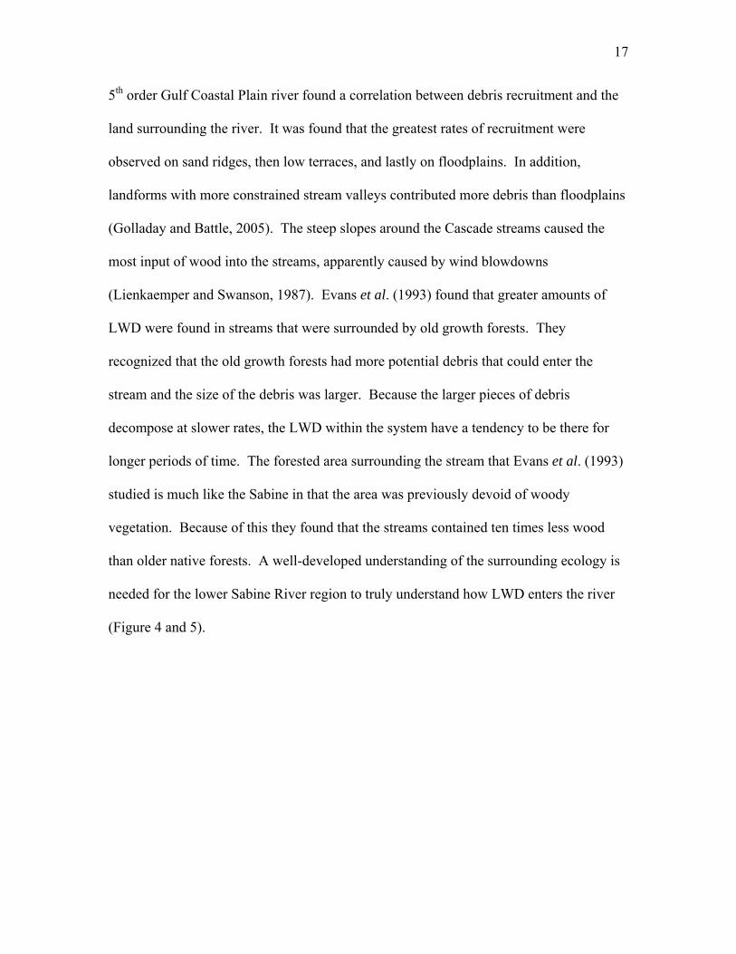
5th order Gulf Coastal Plain river found a correlation between debris recruitment and the
land surrounding the river. It was found that the greatest rates of recruitment were
observed on sand ridges, then low terraces, and lastly on floodplains. In addition,
landforms with more constrained stream valleys contributed more debris than floodplains
(Golladay and Battle, 2005). The steep slopes around the Cascade streams caused the
most input of wood into the streams, apparently caused by wind blowdowns
(Lienkaemper and Swanson, 1987). Evans et al. (1993) found that greater amounts of
LWD were found in streams that were surrounded by old growth forests. They
recognized that the old growth forests had more potential debris that could enter the
stream and the size of the debris was larger. Because the larger pieces of debris
decompose at slower rates, the LWD within the system have a tendency to be there for
longer periods of time. The forested area surrounding the stream that Evans et al. (1993)
studied is much like the Sabine in that the area was previously devoid of woody
vegetation. Because of this they found that the streams contained ten times less wood
is
needed for the lower Sabine River region to truly understand how LWD enters the river
(Figure 4 and 5).
than older native forests. A well-developed understanding of the surrounding ecology

18
Figure 4. Forest surrounding the Sabine River at the Burkeville site on July 21, 2008.

19
Figure 5. Forest surrounding the Sabine River at the Deweyville site on December 19, 2007.
Once the woody debris is within the system’s channel it has several places that it
can go. It can be transported down stream, get caught in a debris jam, or be pushed back
out of the channel. A lot of debris has been found to end up in jams (Figure 6), which
then play an important role in stream morphology and ecosystems (Shields and Nunnally,
LWD Loading
1984). Transient wood from upstream, broken branches, and wood from surrounding
swamps are what Benke s accumulations. LWD
gener
is most likely to get caught in jams. Debris pieces have a greater chance of getting jam
associated than coming to a stop throughout the inter-jam space. Because not all jams
and Wallace (1990) found make up debri
is ally transported downstream by large flood events and it is during this time that it

20
span an entire width of a river, especially in larger rivers, not all pieces will get caught
within a debris jam. The ones that do get caught will stay associated with that jam until
they decay enough to free themselves and be further transported down the river (Bend
and Sias, 2003) or a large enough flood can push them out of the jam.
a
Figure 6. Large woody debrison August 1
ja ower Sabine River, Texas 8, 2008.
In a study on a small British Columbia stream Fausch and Northcote (1992) found
e was greater in areas of the stream where LWD was stuck in a jam as
o areas where no jam . The jam-created pools may then provide
ailable pool habitats rtebrates and other species (Nunnally and
). Local channel w ition, and midchannel bars have been noted
m on the Southern site on the l
that pool volum
compared t s were located
the most av for macroinve
Keller, 1979 idening, depos

21
immediately downstream from a nd Swanson, 1979). Debris jams have a
to occur when a single t inputs several pieces of debris at the same
et al., 1976). Although it would be next to impossible to be able to tell
originated from on the Sabine, it is highly likely that a few
occurred during Hurricane Rita in 2005 led almost directly up the Sabine.
hey
fully understood (Abbe and Montgomery, 1996). On a second-order
woodland stream in Germany, Mutz (2000) found no debris jams in the stretch of stream
that he was studying, even though larger pieces of debris was present. He attributes the
lack of jams to the subdued hydrological regime of the stream. He noted that the larger
wood pieces were stable and could not accumulate into a structure that would capture
smaller floating pieces of wood. The presence of debris jams is most likely due to site-
specific reasons and cannot be categorized by one single universal cause.
Alphanumeric Classification of LWD Montgomery (2008) devised a way to categorize LWD into an alphanumeric
code. Montgomery proposed that if all LWD had a standardized classification then
comparisons between surveys and regions could be achieved. Assumptions could then be
able to be made about the LWD, such as lower classified pieces (smaller LWD) would
jam (Keller a
tendency large even
time (Swanson
where each debris jam
whose path
Golladay and Battle (2005) found that closely monitoring tropical storms and their causes
will give a good indication of when large amounts of debris will enter a river system.
They found that cyclical variations in climate result in periodic pulses of wood debris
entering rivers.
Although some information is known about debris jams, the manner in which t
accumulate is not

22
tend to float and be carried downstream, while higher classified pieces (larger LWD)
ould be more stable and help contribute to a log jam. He went on to say that this
to get
researchers would be able to predict which categories would be “key pieces” or the ones
The classification system is broken into seven categories for length and seven
categories for diameter, totaling 49 discrete classes of LWD (Table 1). LWD length
would get put into a lettered class code of A-G, and wood diameter would get a class
code of 1-7.
TABLE 1. Proposed size classes and codes for the length and diameter of wood debris. Wood length letter code and classes (m)
Wood diameter numeric code and classes (m)
w
classification, along with information on the channel size, would allow researchers
an idea on how the woody debris would affect channel morphology. Furthermore,
that would affect a given stream the most.
(A) 0 to 1 (1) 0 to 0.1
(B) 1 to 2 (2) 0.1 to 0.2
(C) 2 to 4 (3) 0.2 to 0.4
(D) 4 to 8 (4) 0.4 to 0.8
(F) 16 to 32 (6) 1.6 to 3.2
(G) > 32 (7) > 3.2
(E) 8 to 16 (5) 0.8 to 1.6
(Montgomery, 2008)

23
A great amount of research has been performed on the importance of large woody
to stream ecology. The importance of LWD is now more realized and
Summary debris
understood and
unt. What is now needed is a better understanding of the LWD’s role in larger
, because it is probable that LWD plays a vital role in larger river
practices detrimental to LWD such as clearing and snagging must take this importance
into acco
Coastal Plain rivers
systems as well.

24
TASK 2 – CONCEPTUAL MODEL OF LWD DYNAMICS
Task Description - Develop a conceptual diagram of estimated pathways of large organic woody debris through a watershed. Use field work and literature sources to refinthe conceptual model.
e
Basic visual model of large woody debris in Southeastern rivers.
Figure 7 gives a basic visual diagram of LWD dynamics in riverine systems.
RIVER CHANNEL
Instream LWD
Figure 7.
BOTTOMLAND RIPARIAN FOREST UPLAND RIPARIAN FOREST tems
Snags Logging Debris
Live Stems
Snags Live S
TERRESTRIAL BOTTOMLAND
Downed LWD
TRIB
UTA
RY
INFLO
W
MO
RTA
LITY,
DOWNSTREAM OUTFLOW
TERRESTRIAL
Macroinvertebrates
LWD DECAY Bacteria Fungi
WIN
D
CH
AN
NEL
OU
TFLOW
BOTTOMLAND
EXCHANGE CHANNEL
BO
TTOM
LAN
D
BA
NK
ERO
SION
, M
OR
TALITY
W
IND
,
DE
AY
OU
TFLOW
IN-CHANNEL CAY
Macroinvertebrates
C
DECAY
LWD DE Bacteria Fungi

25
This ba
sic
∆Sc = change in woody debris storage ∆x = reach length ∆t = time interval Li = lateral recruitment of LWD within the reach (Lo) wood loss due to overbank depositions in flood events or the abandonment of jams Qi = fluvial transport of wood into the reach Qo = transport of wood out of the reach D = loss of wood due to decay
See Task 1, Literature Review for further details on each of these variables. See
Observed Data and Conceptual Model section in Task 10 Report of Research Findings,
for Sabine River budget calculations.
sic visualization can be further expounded conceptually with a quantitative
framework described by Benda and Sias (2003). This was included in the Literature
Review section under the sub-heading “Large Woody Debris Inputs”. The ba
relationship as summarized by Benda and Sias (2003) is as follows:
∆Sc = [Li – Lo + Qi / ∆x – Qo / ∆x – D] ∆t (9)
Where:

26
TASKS 3 AND 4 – LWD MEASURING TECHNIQUES
Task 3 Description
- Test sampling, measuring, and tracking techniques at three
mainstem test sites described above. In addition to LWD tagging, other measurements that will be recorded include estimates of the number, volume, tree type, and volume of logs in each study unit. A photographic record will be kept to show changes over time.
Task 4 Description - Investigate criteria for test plot selection in bottomland, tributary, and mainstem areas. Set up mainstem sites and use them to evaluate techniques as described in Step 2. As time permits, set up bottomland and tributary test plots and evaluate data collection methods for these areas.
River, Texas. M.S. Thesis, Stephen F. Austin State University, May 2009 149 pp
METHODS OF STUDY
Study Site This study utilized four different sites along the Sabine River (Figure 8). Three
From: Ringer, M.S., Characterizing large woody debris dynamics in the lower Sabine .
sites we
easure
the amount of tim
re originally proposed, with remeasurements of these sites following large
discharges. However, due to the study time constraints and the difficulty in coordinating
pre- and post flow measurements with large discharges (with low flows following for
accurate measurement), a better methodology was employed to answer the questions
about woody debris recruitment rates. Following Hurricane Rita in 2005, the Sabine
River Authority removed all bankside woody debris for a few river miles above the
southeast Texas intake canal. This site, denoted the Southern site, was used to m
e required for woody debris to return to pre-snagging densities. Field
work on the amount of LWD began in Fall 2006 and continued throughout the Summer
of 2008.

27
Figure 8. Four sampling sites located on the lower Sabine River in Texas.
The lower Sabine River, below Toledo Bend Reservoir, establishes the boundary
between Texas and Louisiana. The total drainage area of the Sabine River is 25,267 km²
hysiographic province (Phillips, 2003). The soils surrounding the river were mostly
light-colored, fine, sandy loams with subsoils that contain loamy sand to plastic clay in
and the area has a humid subtropical climate lying in the Gulf Coastal Plain
p
texture and yellow to red in color (Figure 9).

28
Figure 9. Sand bar on the lower Sabine River, Texas.
The vegetation was mostly composed of pines with a hardwood understory. Much of the
surrounding land had previously been cultivated and is now used for pasture or has been
reforested, either naturally or by planting (Phillips, 2003). All four study sections were
Previous studies conducted on the lower Sabine River found that due to the
almost regular daily discharge of water from the reservoir, the lower Sabine had been
affected little by the impounding of the upper portion of the river. At the portion of the
river near Burkeville, Texas there was evidence of bank erosion, input of large woody
debris, and sandbar migration. Evidence in the area also showed that the floodplain was
continuing to accrete, which indicated a normal river balance. Further downstream at the
located on the lower Sabine River (Figure 8), south of Toledo Bend.

29
Bon Wier site, the area had abundant amounts of woody debris, eroding banks, and tilted
trees that could be potential future woody debris. Evidence was also found of a
downstream migration of a large sandy point bar. At a third site near Deweyville,
ts of LWD at
e bank base and in the channel, and undercut live trees on the bank (Phillips, 2003).
The three un-snagged sites were chosen based on the low human disturbances in
each section. Homes were spread along the entire length of the Sabine, and it was
essential to pick three sites that did not have a house situated within the study section.
The most southern of the three un-snagged sites was located near Deweyville, Texas
(30°18’94”N, 93°44’68”), 2.24 kilometers north of the Highway 12 bridge (Figure 11).
This site was characterized by low banks usually ranging from 0-10 feet, with active
cutbanks and migrating sand bars (Figure 10).
The middle site was located near Bon Wier, Texas (30°42’57”N, 93°37’10”W),
5.21 kilometers south of the Highway 190 bridge (Figure 13). The Bon Wier site had
slightly higher banks than the Deweyville site, and it also contained active cutbanks and
migrating sand bars (Figure 12).
sandbars were found that were actively prograding, tilted trees, large amoun
th

30
Figure 10. Characteristic Deweyville site on the lower Sabine River, Texas.

31
Figure 11. The Deweyville woody debris sampling site on the lower Sabine River, Texas

32
Figure 12. Characteristic Bon Wier site on the lower Sabine River, Texas.

33
Figure 13. Map of the Bon Wier site on the lower Sabine River, Texas.
The most northern site was located near Burkeville, Texas (31°2’67”N, 93°31’21”W),
3.68 kilometers south of the Highway 63 bridge (Figure 15). The Burkeville site was
most unique in that its cut banks could be as high as 30 feet tall. As with the other two
sites it contained active migrating sand bars and also had cutbanks, which leads to LWD

34
input (Figure 14). The lower Sabine had LWD in large amounts of its stretches so
was not much concern about choosing a specific site based on its amount of LWD
there
.
Figure 14. Characteristic Burkeville site on the lower Sabine River, Texas.

35
Figure 15. Map of the Burkeville site on the lower Sabine River, Texas.
An additional site, the Southern site (30°16’87”N, 93°42’37”W), was located 8.86
kilometers south of the Highway 12 ometers north of the river split
ng
bridge and 2.29 kil
(Figure 17). Different from the other three sites, the Southern site was snagged followi
Hurricane Rita in 2005 (Figure 15). This site provided a good indication of how long it
took for LWD to be replenished in the Sabine.

36
Figure 16. Characteristic Southern site on the lower Sabine River, Texas.

37
Figure 17. Map of the Southern site on the lower Sabine River, Texas.
ooding summer power generation
schedules, water was released Monday through Friday and then shut off for the weekends
Field Methods Data and samples were collected the same way at each of the four study sites.
The most ideal time to study LWD was when the river was low enough to find a high
percentage of LWD. Flow rates of the Sabine were regulated by the Toledo Bend
Reservoir throughout the year (Table 4). Under non-fl

38
when power demand was lower. Due to this baseflow regimen, the best days to sampl
for LWD was early in the week. As water levels rose many pieces of LWD were
submerged and measurement was not possible. Prior to sampling, river stage was
evaluated from United States Geological Survey (USGS) gauging stations. For
Burkeville and Bon Wier, sampling would only be conducted when the gauge height w
around 4.5 m (15 ft) or below. The Deweyville and Southern site would be sampled if
they were around 6.1 m (20 ft) or below. Each piece of LWD was located either in the
channel of the river or on the bank tha
e
as
t had a minimum diameter of 10 cm and a
minimu length of 2 m. Each piece was tagged with a specific number using a
number on the metal tag was recorded on
and was used to identify the p measurement phase and for
ssible future measurements. The same nu ed on the log using
ather-proof spray paint (Figure 18).
m
numbered metal tag, hammer, and nails. The
the data sheet iece during the
po mber was then spray paint
we

39
Figure 18. Tagged and painted LWD.
Log length and top and butt diameters were then measured with a tape and
n was
unknown was recorded on the data sheet. The level of decay was selected based on five
the
as intact
but the twigs were absent. An indictor of 3 indicated only traces of bark were left on the
he fourth indicator meant that the bark was absent with some holes and openings
was darkened. The last category would indicate that the bark was absent
nd the wood was irregularly shaped and was darkened.
recorded. The species of the LWD was identified when possible, but identificatio
often difficult on highly decayed specimens. When species could not be determined,
categories (Table 2). An indicator of 1 meant that no sign of decay was visible on
piece, all bark and branches were intact. An indictor of 2 meant that the piece w
wood. T
and the wood
a

40
TABLE 2. Degree of decay classes of LWD.
Characteristics Degree Class
I Bark intact, twigs present
II Bark intact, twigs absent
ions
ned
V Bark absent, irregular shape, wood
III Only traces of bark, with abras
IV Bark absent, some holes, wood darke
Next, bank orientation was determined. A bank orientation of 0° meant that the
root wad was facing upstream and the LWD was parallel to the bank; a bank orientation
n of 180°
as noted
with a yes or no, as well as the presence of branches. Identification of LWD origin was
attempted but was not always possible. The categories for origin were local riparian,
upstream import, and non-determinable. Identification of the potential source was also
attempted and classified as windthrow, windsnap, cut, and non-determinable. The origin
and potential source was sometimes difficult to determine. If insufficient information
able, a non-determinable was marked on the data sheet. It was then noted if the
individual piece, jam-associated, or a fallen tree. Figure 19 shows two
latively large piece causes many others to get caught. Finally, each LWD was
age contact zone. A category for zone 1 indicated that the piece was
flow contact area, zone 2 indicated that it was within the bank-full
of 90° indicated the log was perpendicular to the channel; and a bank orientatio
indicated the LWD was facing downstream. Then, the presence of a root wad w
was avail
LWD was an
common ways the LWD was distributed. Often, wood was found in a jam, where one
re
classified into a st
sitting in a low

41
channel, zone 3 indicated that it extended over the bank full channel, and zone 4
indicated that LWD was beyond the bank-full channel.
Figure 19. Common LWD distributions (Gippel, 1995).
arked with its identifying number. An increment borer was used to collect samples, but
hile the increment borer provided a more representative sample
ould swell in the borer, making it impossible to extract the sample without oven drying.
e nt parts of the wood were collected. Most LWD locations were then
For every piece of LWD, a sub-sample was collected and placed inside of a plastic bag
m
a handsaw, chainsaw, or hatchet was used to remove a sample when the corer failed
(Figure 20). W
throughout the log, it did not work well with fully saturated wood, since the samples
w
All collected samples attempted to represent both inner and outer parts of the tree, to
ensure diff re
marked with a Magellan GPS unit and a picture of the piece was taken. However, GPS
42
coordinates often were not accurate enough for precise location within each jam or even
reach, so these data had limited utility.
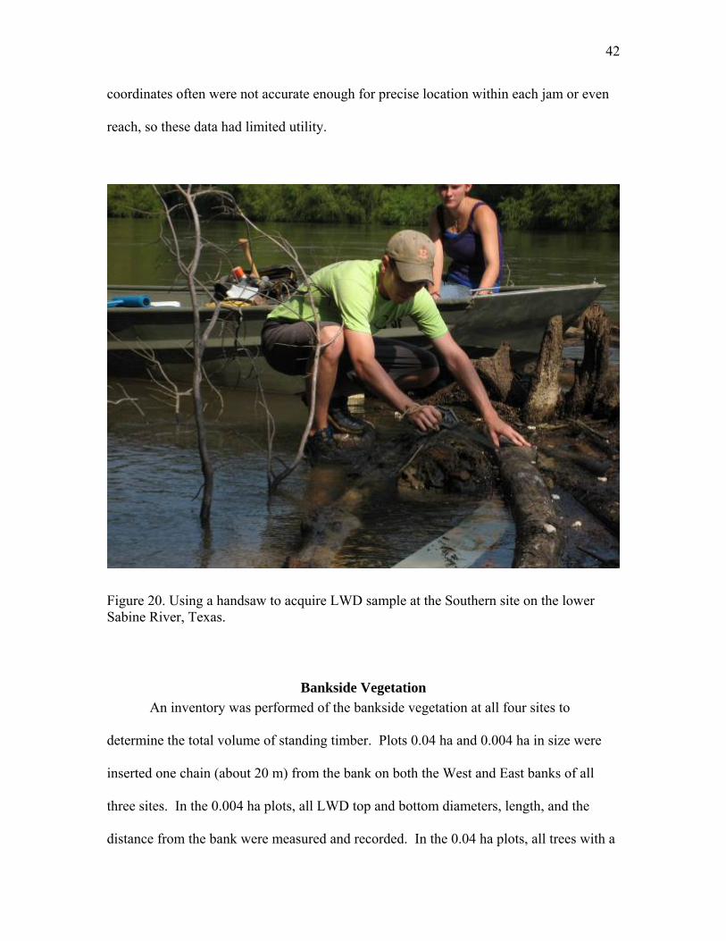
Figure 20. Using a handsaw to acquire LWD sample at the Southern site on the lower
Bankside Vegetation An inventory was performed of the bankside vegetation at all four sites to
determine the total volume of standing timber. Plots 0.04 ha and 0.004 ha in size were
inserted one chain (about 20 m) from the bank on both the West and East banks of all
three sites. In the 0.004 ha plots, all LWD top and bottom diameters, length, and the
distance from the bank were measured and recorded. In the 0.04 ha plots, all trees with a
Sabine River, Texas.

43
minimum of 10 cm diameter at breast height (DBH) were recorded. DBH, total tree
eight, and distance from the bank were measured and recorded. Instruments used for
ice Research Paper SE-
293, titled “Stem Cubic-Foot Volume Tables for Tree Species in the Deep South Area
Each LWD sub-sample was brought to the lab and wet mass was measured. It
was then oven-dried at 105° C to a constant mass. The piece was then reweighed and the
dry mass was recorded. Percent moisture of each sample was then found by:
[(wet mass – dry mass) / wet mass] x 100.
Each sample piece was then sealed in paraffin wax. The paraffin wax helped to hold
together the pieces of wood that showed high amounts of decay. It also prevented
volumetric changes when determining sample volume by water immersion. After the
piece was dipped in wax it was reweighed to get its weight after waxing.
Due to the irregularities of each piece, a simple volume calculation (length x
width x height) would not suffice. Instead, after coating each piece with wax they were
immersed in water to determine displacement. The amount of water displaced was then
measured resulting in volume, based on Archimedes Principle. A dish was used to catch
overflow, a 1000 ml beaker for the fill container, a graduated cylinder to measure the
water overflow, a metal probe for inserting the sample, and lastly a wash bottle to slowly
get the water level to its maximum level in the fill container. The fill container was
h
both set of plots were a tape measure and a diameter tape. Stand tables were constructed
sing the United States Department of Agriculture Forest Servu
(Clark and Souter, 1996). The Girard Form Class for the pines was 81 and for the
hardwoods was 79.
Sample Analysis

44
placed inside of the overflow dish and filled to the rim. The wash bottle was used to
slowly raise the water to the very top of the container, just shy of breaking the water’s
surface tension. The metal probe was inserted into one sample piece and inserted slowly
into the water. The water in the overflow dish was then poured into a graduated cylind
and the sample’s volume was recorded in milliliters. It was possible to then find each
sample’s density using:
mass / volume.
Using the mass of each sample after it had been dipped in wax was important because
the changes the wax made to the mass of each piece. Because each of the four sample
sites were different lengths, it was important to find the mass and volume per unit reach
er
of
.
45
TASK 5 – DECAY ANALYSIS
Task 5 Description
- Conduct decay analysis and test decay models for application in
a suitable decay function will be determined. From this, the expected time to decay in years will be calculated.
study was to form the basis for analyzing decay rates in the current study. Results from
State University (SFASU), and Texas Water Development Board (TWDB) personnel.
he decay of LWD limits the
amount of time that it will spend within a stream system. Previous studies show that it
within the stream channel will break down into moveable pieces because of the force of
an equation for wood decay:
where k is annual decay loss and S is the storage of living and dead wood in a landslide
t in
jams and usually exit the stream as a floatable piece.
Texas. Determine degree of decay from woody debris specimens based on degree of penetration, sample specific gravity, species, and size. Terrestrial decay rates will be modified for aquatic conditions. The decay rate constant for
A detailed experiment involving woody debris decay rates by species and degree
of stage contact was conducted a few years ago, funded by the U.S. Forest Service. This
that study were not available, in spite of efforts by U.S. Forest Service, Stephen F. Austin
However, it was determined that a basic understanding of decay rates, decay dynamics,
and decay class would be adequate for fulfilling this task. T
will lose 2 to 7% of mass per year (Spies et al., 1988). The pieces of LWD that are
the stream (Benda and Sias, 2003). Bilby et al. (1999) found that wood submerged
decayed at a 2 to 3% rate, depending on the tree species. Harmon et al. (1986) developed
D(x,t) = kdSs, (8)
d s
area. The study goes on to show that loss of mass creates loss of strength, which breaks
up the LWD into smaller pieces. The smaller pieces have a harder time getting caugh
46
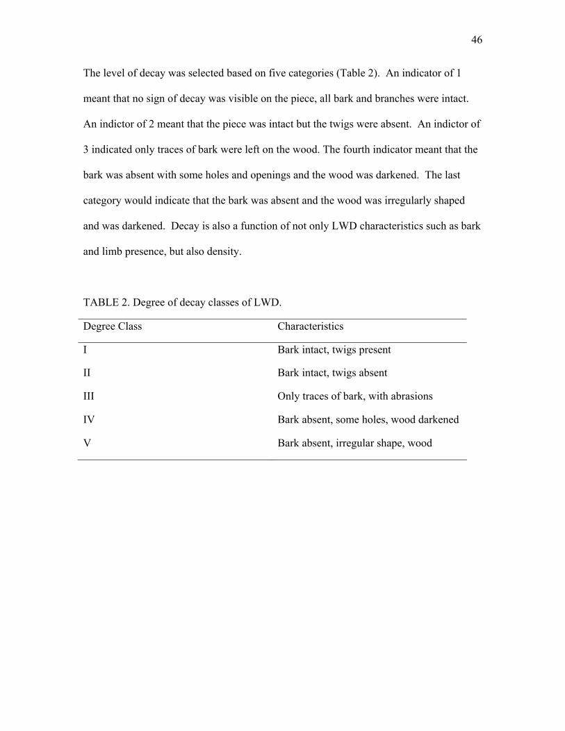
The lev
of
Degree Class Characteristics
el of decay was selected based on five categories (Table 2). An indicator of 1
meant that no sign of decay was visible on the piece, all bark and branches were intact.
An indictor of 2 meant that the piece was intact but the twigs were absent. An indictor
3 indicated only traces of bark were left on the wood. The fourth indicator meant that the
bark was absent with some holes and openings and the wood was darkened. The last
category would indicate that the bark was absent and the wood was irregularly shaped
and was darkened. Decay is also a function of not only LWD characteristics such as bark
and limb presence, but also density.
TABLE 2. Degree of decay classes of LWD.
I Bark intact, twigs present
II Bark intact, twigs absent
III Only traces of bark, with abrasions
IV Bark absent, some holes, wood darkened
V Bark absent, irregular shape, wood

47
TASK 6 – STATISTICAL ANALYSIS Task 6 Description - Develop appropriate statistical techniques to test and verify data collected for LWD budgets.
tests were used to
determ
no a-
e
tion,
HO: There is a uniform distribution of the LWD in the degree of decay of LWD.
Decision Rule: reject HO if x is ≥ to the critical value; otherwise, do not reject.
HO: There is a uniform distribution of the LWD in the branch presence of LWD.
Decision Rule: reject HO if x is ≥ to the critical value; otherwise, do not reject.
HO: There is a uniform distribution of the LWD in the potential source of LWD.
Decision Rule: reject HO if x is ≥ to the critical value; otherwise, do not reject.
Origin
HA: Not HO. Rule: reject HO if x2 is ≥ to the critical value; otherwise, do not reject.
Most of the data collected were categorical, so chi-square
ine if any category had a uniform distribution. A uniform distribution was chosen
because no LWD research had been performed on the Sabine River, so there were
priori assumptions about expected distributions. The chi-square tests were used to
examine eight categories within the individual sites. The categories tested were: degre
of decay, branch presence, potential source, origin, bank orientation, root wad, posi
and stage contact. SAS was used to run the chi-square tests. The following hypotheses,
decision rules, and test statistics were used to test the eight categories:
Degree of decay
HA: Not HO. 2
Branch presence
HA: Not HO. 2
Potential Source
HA: Not HO. 2
HO: There is a uniform distribution of the LWD in the origin of LWD.
Decision

48
Bank oHO: There is a uniform distribution of the LWD in the degree bank orientation of LWD.
Decision Rule: reject HO if x is ≥ to the critical value; otherwise, do not reject.
HO: There is a uniform distribution of the LWD in the root wad of LWD.
Decision Rule: reject HO if x is ≥ to the critical value; otherwise, do not reject.
HO: There is a uniform distribution of the LWD in the position of LWD.
Decision Rule: reject HO if x is ≥ to the critical value; otherwise, do not reject.
HO: There is a uniform distribution of the LWD in the stage contact of LWD.
Decision Rule: reject HO if x is ≥ to the critical value; otherwise, do not reject.
ategories tested were: potential source, origin, bank orientation, root wad,
position
Position
HA: Not HO.
12.592 (p<0.0001), reject Ho and conclude that some association exists between LWD
Degree of Decay sites.
HA: Not HO.
rientation
HA: Not HO. 2
Root wad
HA: Not HO. 2
Position
HA: Not HO. 2
Stage contact
HA: Not HO. 2
Next, contingency tables were developed to test eight categories between the
sites. The c
, stage contact, degree of decay, and branch presence. The following hypotheses,
decision rules, and test statistics were used to test the eight categories:
HO: There is no association between the position of LWD and the four study sites.
Decision Rule: reject HO if x2 is ≥ to 12.592; otherwise, do not reject. Since 130.6693 >
position and the four study sites.
HO: There is no association between the degree of decay of LWD and the four study

49
Decision Rule: reject HO if x2 is ≥ to 21.026; otherwise, do not reject. Since 29.4311 >
degree of decay and the four study sites.
HO: There is no a
21.026 (p=0.0034), reject Ho and conclude that some association exists between LWD
Branch Presence ssociation between the presence of branches on LWD and the four study
sites. HA: Not HO. Decision Rule: reject HO if x2 is ≥ to 7.815; otherwise, do not reject. Since 2.7287 < 7.815 (p=0.4354), do not reject Ho and conclude that no association exists between LWD branch presence and the four study sites. Root Wad Presence HO: There is no association between the presence of root wads on LWD and the four study sites. HA: Not HO. Decision Rule: reject HO if x2 is ≥ to 7.815; otherwise, do not reject. Since 31.9060 > 7.815 (p<0.0001), reject Ho and conclude that some association exists between LWD root wad presence and the four study sites. Stage Contact HO: There is no association between the stage contact of LWD and the four study sites. HA: Not HO. Decision Rule: reject HO if x2 is ≥ to 16.919; otherwise, do not reject. Since 38.9937 > 16.919 (p<0.0001), reject Ho and conclude that some association exists between LWD stage contact and the four study sites. Potential Source HO: There is no association between the potential source of LWD and the four study sites. HA: Not HO. Decision Rule: reject HO if x2 is ≥ to 12.592; otherwise, do not reject. Since 87.8092 > 12.592 (p<0.0001), reject Ho and conclude that some association exists between LWD potential source and the four study sites. Bank Orientation HO: There is no association between the bank orientation of LWD and the four study sites. HA: Not HO. Decision Rule: reject HO if x2 is ≥ to 12.592; otherwise, do not reject. Since 46.4740 > 12.592 (p<0.0001), reject Ho and conclude that some association exists between LWD bank orientation and the four study sites.

50
Origin
O: There is no association between the origin of LWD and the four study sites.
es
LWD volume
.63; otherwise, do not reject. Since 7.03 > 2.63 the volumes are significantly different.
Bankside VegetHo: µBurkeville = µHa: not HoDecision Rule: reject H if F is ≥ to 3.01; otherwise, do not reject. Since 0.89
lu ntly
HHA: Not HO. Decision Rule: reject HO if x2 is ≥ to 7.815; otherwise, do not reject. Since 52.8256 > 7.815 (p<0.0001), reject Ho and conclude that some association exists between LWD origin and the four study sites.
An ANOVA test was used to compare the bankside volume and LWD volume of
each site to see if the volume amounts were significantly different. Comparing the sit
to one another gave an idea of how much mass per unit stream length the lower Sabine
River contained. It also showed how much volume there was per unit stream length.
When comparing the 3 un-snagged sites to the 1 snagged site the tests showed if snagging
had affected the area at all. The following hypotheses were used to test the volumes of
LWD and bankside vegetation:
Ho: µBurkeville = µBon Wier = µDeweyville = µSouthern
Ha: not Ho Decision Rule: reject HO if F is ≥ to 2(F=0.0001), reject Ho and conclude that
ation volume Bon Wier = µDeweyville = µSouthern
O< 3.01 (F=0.4118), do not reject Ho and conc de that volumes are not significadifferent.
51
TASK 7 – LWD STORAGE
Task 7 Description
- Investigate methods to determine residence time for storage locations in LWD budgets. Methods that should be considered include those described by Hyatt and Naiman, 2001, and Abbe et al., 2003.
According to Hyatt and Naiman (2001), there are three general methods for
determining woody debris age and thus residence time for storage locations. These
included dendrochronology, radiocarbon dating, and the use of dependent vegetation.
First, dendrochronology could be employed. This would involve removing increment
cores from both instream LWD and from standing riparian trees to develop a master
chronology for crossdating LWD cores. Ring widths vary based on annual variations in
rainfall, temperature, and other climatic factors. It was assumed that patterns in ring
widths from the master chronology matched up with LWD, thus not only tree age could
be determined, but also when the tree died and an estimate of how long the LWD has
been in the river. Hyatt an
d Naiman (2001) employed this technique in the Queets River
in Was ers
ort lifespans.
For the lower Sabine River, using dendrochronology as a dating technique would
be a challenge. First, the most reliable trees for this work would be members of the
genus Pinus. Loblolly pine (Pinus taeda) was only rarely found in the bankside
inventories or as LWD specimens. About 4.2 trees per hectare pine were found in the
riparian area, versus 50 trees per hectare hardwood at the Bon Wier site, with no pines
hington. This riparian area had long-lived conifers that provided the research
with master chronologies dating back to the 14th century A.D. Also, these conifers were
found in the river channel. Hyatt and Naiman (2001) found that hardwoods were
unreliable for dendrochronology due to missing or indistinct rings, rings that failed to
correlate between trees or between cores from the same tree, or too sh

52
found at the other three. Dominant riparian species included oaks (Quercus), which have
me potential for developing a master chronology, though oaks are difficult for several
issing rings. Many of the best specimens
were removed in logging operat ve missing or indistinct rings.
aldcy
w
y Hyatt and Naiman
ore
re difficult than in the
ollection from LWD would be needed to th the necessary matches.
The ne ni s ya i w ra
dating. This technique worked well f de s. e
14C concentrations after the mid-1960s from nuclear testing resulted in som
ology,
decay class, dependent vegetation, and age of adjacent logs to aid in calibration to
so
reasons. First, they have dense wood that is difficult to bore and extract an intact core.
hey often have heart rot which results in mT
ions. Finally, oaks often ha
B press (Taxodium distichum), while a conifer, is a notoriously poor species for
dendrochronology due to false and incomplete rings. Furthermore, like with the oaks,
many of the oldest trees were harvested many years ago and the remaining trees were
young. Other species like willow (Salix nigra), cottonwood (Populus deltoids), or tallo
tree (Sapium sebiferum) were often short lived and also subject to rot. A final concern
was the difficulty in boring saturated trees. While not mentioned b
(2001), we found that boring saturated, higher density logs resulted in the increment c
swelling in the bore bit, making core extraction impossible without first oven drying it.
This is the main reason saws were used to collect specimens rather than increment borers.
While dendrochronology on the lower Sabine would be mo
Queets River, it is not impossible. Collection of multiple bores from each key tree along
with cookies from selected trees would help to establish the master chronology. Cookie
c en make
tt and Na
r, pre 1960 specim
xt tech que discu sed by H man (2001) as using
Ho
diocarbon
levated or ol en wever,
atmospheric e
challenges. Hyatt and Naiman (2001) used other techniques like dendrochron

53
de ine whether the specimen was on the rising or trailing end of the bomb decay
curve. This technique may be successfully employed on the lower Sabine, especially
older, more decay resistant species and merits additional exploration. For LWD recru
post-1960, additional calibration work would be necessary.
The final, and least reliable technique employed by Hyatt and Naiman (2001) was
the use of dependent vegetation which has grown up on debris jams. They found this
be the least reliable indicator of residence time. Many specimens that had 1-5 year old
vegetation were found to have been in the channel more than 20 years. Furthermore,
several of the oldest pieces had any dependent vegetation while younger specimens
Very little dependent vegetation was observed on the Sabine LWD jams, and due to t
difficulties mentioned by Hyatt and Naiman (2001), this is not likely to be an effecti
method for determining residence time.
Abbe et al. (2003) reported on reintroducing wood into streams and how
rehabilitation of fluvial ecosystems was best accomplished by placing wood in the
appropriate hydrologic or geomorphic setting. When key members become established,
jams can accumulated and lasted for many years. The most important variable for key
member stability was having an attached root wad with a 2 m radius. This root wad
raised the center of mass more than five times the tree’s diameter and the root mass acte
like a plow, increasing resistance. Often these root wads may still be attached to the
bank, further increasing key member stability. Abbe et al. (2003) concluded that log
jams can be successfully reestablished for greater than 20 year floods, control bank
erosion without exacerbating local flooding, and can dramatically enhance physical
habitat such as pool frequency, depth, and cover.
term
for
ited
to
did.
he
ve
d
54
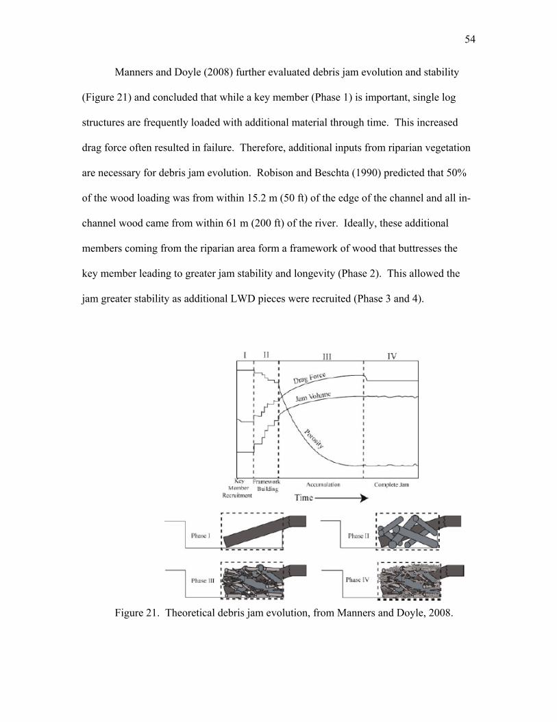
Manners and Doyle (2008) further evaluated debris jam evolution and stabili
(Figure 21) and concluded that while a key member (Phase 1) is important, singl
structures are frequently loaded with additional material through time. This increased
drag force often resulted in failure. Therefore, additional inputs from riparian vegetation
are necessary for debris jam evolution. Robison and Beschta (1990) predicted that 50%
of the wood loading was from within 15.2 m (50 ft) of the edge of the channel and all in
channel wood came from within 61 m (200 ft) of the river. Ideally, these additional
ty
e log
-
members coming from the riparian area form a framework of wood that buttresses the
jam stability and longevity (Phase 2). This allowed the
m gre
key member leading to greater
ja ater stability as additional LWD pieces were recruited (Phase 3 and 4).
Figure 21. Theoretical debris jam evolution, from Manners and Doyle, 2008.

55
TASK 8 – LWD TRANSPORTATION Task 8 Description - Investigate methods for calculating transportation rates for LWD budgeEvaluate the potential of theoretical calculation methods corrected with field data described drick and G 2000, and Ha al, 2002.
Braudrick and Grant (2000) reported on a series of flum designed to
test simple entrainme ed o moving water on logs. No
consideration was given to bank or vegetative effects in their experiments. Furthermore,
LWD was modeled as geometrically regular pieces smooth bores and straight without
crooks or limbs. Therefore, their model provides theoretical minimum conditions
required to initiate LWD transportation. In general, even in this simplified experiment,
they found that movement of wood in streams was far more complex than sediment due
to the cylindrical bole, irregular rootwad large size relative to channel dimension, and
opportunity for various orientations relative to flow. Furthermore, unequal forces act on
t parts of the log, including flotation and wood can move in different ways,
including sliding, rolling, pivoting, and floating. In general, these researchers found that
diameter was the most important factor determining piece stability, assuming piece length
llel to flow increased stability by 39%,
stly due to the tance offered ediments just downstream of the LWD
structing movem nt. Adding a rootwad increased piece stability by 71%. The
mework of rootwads increased drag forces and enhanced
piece st
ts.
by Brau rant, ga, et
e experiments
nt models bas n the force of
differen
was less than channel width. Orienting para
mo resis by s
ob e
irregular shape and open fra
ability. These researchers did not report on varying discharge and velocity, nor
did they provide estimates of how differing flow variables would affect LWD of different
sizes.

56
In general, their flume experiment would “scale up” to a river 39.3 m wide by
0.71 m deep. These were reasonable conditions for the lower Sabine, though their model
t uch larger than that fo bine .32
By site, Burkev ad the larges meter of 0.41 m and it was significantly
ter than the other 3 sites. Lengths in this study were also greater, ranging from 11.8
.6 m versus a m n piece length he lower Sabine of 6.8 m. In all cases, piece
ngth was less than channel width. In conclusion, Braudrick and Grant (2000) presented
a theor
D
uld be limited,
Due to these restrictions, Haga et al. (2002) reported on LWD transport in small
untain streams in Japan. These streams lacked the sorts of obstructions that that
late the assump ns of Braudrick and Grant’s (2000) model. Furthermore, all of the
D pieces in Haga et al.’s (2002) experiment were less than the bankfull width. In
eneral, they found that flow depth as well as the magnitude and sequence of flows were
importa
moved, LWD was not as much flow limited as limited by jam spacing. Therefore, jams
had a steeper channel slope and thus greater velocities. Furthermore, their piece sizes
were the equivalen to 1-1.5 m, m und in the Sa River of 0
m. ille h t mean dia
grea
to 23 ea in t
le
etical model that could reasonably predict LWD transport conditions. However,
additional model development would be required before actual field conditions could be
put into the model for the Sabine River to estimate at what discharges key pieces of LW
may become mobile. Furthermore, the actual utility of such a model wo
since these models do not account for resting logs trapped by instream obstructions like
logjams.
mo
vio tio
LW
g
nt factors for LWD transport and retention. They found that trapping
mechanisms like jams were very important, since often the potential transport distance
due to flow was greater than the distance between jams. Thus, in terms of distance

57
played a crucial role in LWD entrainment. As with Braudrick and Grant (2000), Haga et
al. (2002) assumed unif
orm piece shapes, and recognized that the shape of the piece, and
actual
sport.
presence of a rootwad and limbs would likely be most important for understanding
LWD tran

58
TASK 9 – LWD DOMINANT DISCHARGE
Task 9 Description
- Inv igate the requirements to develop a dominant discharge for woody debris and provide example calculations. This is an untested concept with little literature support, but wo follow the geo rphic concept o ominant discharge for inorganic sediment.
noted above, B udrick and Gran 2000) observed that the movemen f wood
in stre was far more complex than sedim ical bole, irreg r
rootwad large size relative to channel dimension, and opportunity for various orientations
relative to flow. In that experiment, they did not account for the many other variables
that affect woody debris t sport, like parti burial, presence of limbs, irregular shapes,
jam entrainment, variatio in streambanks channel profiles, etc. Therefore, e
discharge estimates would be much lower t
natural system. For example Haga et al (2002) assumed that movement occurred when
the no ensional forc ) > 1, that was the hydraulic force (F) was greater than log
resista R), such that F/R, or
Ψ = 2C
est
uld mo f d
As ra t ( t o
ams ent due to the cylindr ula
ran al
ns and thes
h what would actually be encountered in a an
n-dim e (Ψ
nce ( Ψ =
dρCH
2h*sin α (k sinθ + β(h*) cos(θ)h* gk – 4β(h*)ρ) α – sin α
ere: Cd = drag coefficient between log and water k = constant depending on log ρ = water density θ = angle of log relative to flow CH = Chezy’s coefficient g = acceleration due to gravity h = water depth σ = channel bed slope angle α = channel bed slope µ = coefficient of friction between log and
channel bed
The relationship is represented graphically in Figure 22.
(πσ (µ cos ) Wh

59
Figure 22. Relationship between flow and depth for LWD transport, from Haga et al. (2002
relationship assumed that the critical point for movement occurred when the
e
were
.
tes of
).
This
water depth was about one third the diameter of the log. For simple wooden cylinders in
unobstructed streams, this theoretical relationship was found by Haga et al. (2002) to b
reasonable. However, in the lower Sabine with actual LWD, the observational data
found to be untenable. For example, the mean diameter was around 30 cm (12 in), and
during all of the measurement periods, the depth was several times this. By this model,
all of the pieces of LWD should have been mobile during low flows. However, they
were not due to the irregularity of the pieces, presence of root wads, and jam associations
The utility of this model would therefore be limited for providing reasonable estima
what stream discharge would be required to begin mobilizing key LWD elements and
thus jam movement. Haga et al (2002) acknowledged this when they indicated that the

60
limiting factor for LWD movement was not the energy of the stream, but the resistance
provided by obstructions.
However, there clearly is some dominant discharge that will result in LWD
mobility. For this to happen, the key LWD elements would have to be mobilized in order
to destabilize the jam. The force required for this would mostly depend on the degree of
entrainment of the key LWD elements. Therefore, developing a general model for jam
mobility in lower Coastal Plain Rivers will require additional study.

61
TASK 10 – REPORT OF RESEARCH FINDINGS
Task 10 Description
– Submit report and summary of findings. Assemble and present
understanding of LWD in rivers of Texas.
m3.
00 kilometers,
Dewey
d
d
Difference) for LWD and bankside vegetation for each study site along the lower Sabine
Count (m3)
Reach
(km)
per
(m3/km)
Tukey
for LWD
Bankside
(m3ha-1)
ing for kside
Vegetation
results to date from the project. Describe research needed in future years to advance the
LWD Mass and Volume
The Burkeville site contained 93 logs, Bon Wier had 95, Deweyville had 119, and
the Southern site had 67 logs (Table 3). The Burkeville site had 98.94 m3, the Bon Wier
site had 29.67 m3, Deweyville contained 49.43 m3, and the Southern site had 30.43
The length of the Burkeville site was 1.16 kilometers, Bon Wier was 1.
ville 1.06 kilometers, and the Southern site was 2.29 kilometers. The total length
of the river from the dam to the river split was 147.58 kilometers.
The volume of LWD was significantly (p=0.0001) different between the four
study sites. LWD loads did not increase further south, as was expected. Burkeville ha
similar counts of LWD, but its volume was much higher, indicating that the pieces foun
at Burkeville were much bigger than the LWD at the other sites.
TABLE 3. Total counts, volume, and ANOVA results (using Tukey’s Honest Significant
River.
LWD LWD
Volume Length
Volume
Length Grouping Volume
Tukey Group
Ban
Burkeville 93 98.94 1.16 85.29 A 349.9 ABon Wier 95
Deweyville 1129.67 1.00 29.67 B 248.1 A
9 49.43 1.06 49.63 B 407.1 ASouthern 67 30.43 2.29 13.29 B 476.3 A
Mean values with the same letter are not significantly different at α = 0.05

62
Tables 16-19 present details for the standing vegetation at the Burkeville, Bon
Wier, Deweyville, and Southern sites, respectively. From the results of the standing
vegetation it was expected that Deweyville would have the highest volume of LWD
because it had the highest amount of standing vegetation around it, but again that was not
the case. The differences were due to Burkeville having very large amounts of vol
LWD originating from its banks or be
ume of
ing or being recruited from upstream. Another
explana
ees
tive
with m
a
le 3).
tion could be found by examining at Phillips’ (2003) study of the lower Sabine
River where he examined the effects of Toledo Bend Reservoir on the river downstream
of the dam. In his study, Phillips (2003) reported significant bank erosion, sandbar
migration, and LWD inputs at the Burkeville site. The banks at Burkeville were the
steepest of his three study sites, and were heavily eroded, resulting in greater LWD
inputs. Phillips (2003) reported that the left bank was characterized by many fallen tr
and bank eroded trees. He observed that overall this section of the river was very ac
any migrating sandbars and higher rates of bank erosion. On the other hand,
Phillips (2003) found that near the Bon Wier section of the river there was less channel
erosion. At the Deweyville site, Phillips (2003) observed that the overall river takes on
completely different form, with lower banks and fewer sandbars. He mentioned that the
left bank of the site had numerous amounts of LWD and tilted trees and the right bank
had former bank scarps with abundant LWD at the bank base and in the channel. The
LWD loadings in this study were similar to those observed by Phillips (2003) (Tab
Looking at local geomorphic features and understanding how the river was affecting the
banks at the local sites were the best way to explain the LWD loading differences. Not
only is there more active erosion at the Burkeville site, the site also was characterized by
63
vegetation standing close to the channel, which explained why the high volumes of
LWD. The Bon Wier site contained the least amount of LWD volume and was
mentioned by Phillips (2003) that the banks were not very active and the riparian forest
was less dense. The Deweyville site contained a LWD volume that was in the middle of
the Burkeville and Bon Wier sites and the activity of its bank also lay somewhere in the
middle of the other two sites but had a well-stocked riparian forest. LWD loading was
best explained by the combination of bank erosion rates and riparian forest density.
Flow Rates and Stream DepthWoody Debris Dynamics
Flow rates and river depth data were obtained for the sampling periods from
USGS flow data (Table 4). The Deweyville site (USGS 08030500) was sampled on
October 19, 2007, November 9, 2007, and was completed on December 19, 2007. The
values shown for both flow rates and stream depth are an average of what occurred
sampling date. For Deweyville’s data the values for all three sampling dates were
averaged to get one overall value. Bon Wier (USGS 08028500) was the second site
sampled and it occurred on July 14, 2008. The sampling of Burkeville (USGS 08026000)
occurred on July 21, 2008 and the Southern site (USGS 08030500) was completed on
August 18, 2008.
on the

64
TABLE 4. Averages of stream discharge and stream depth at the four study sites along
Burkeville Bon Wier Deweyville Southerthe Lower Sabine River during sampling dates.
n
Discharge 129.00 45.30 33.10 (m3/s)
177.00
Depth 5.18 4.80 4.55 6.4
July 21, 2008 July 14, 2008
October 19,
December 19, 2007 2008
(meters) 6
Sampling Date November 9, and August 18,
Categorical Counts
All of the sites showed similar decay class counts to one another.
weyville had the most amount of LWD in the third
category, and only the Southern site ha st counts in the fourth category (Table 5).
Decay Class 5 co nts of LWD because the material was decayed,
broken, and even n river
TABLE 5. Degree of decay counts f udy sites along the lower Sabine River. Decay Class Bon W Deweyville Southern
Burkeville, Bon Wier, and De
d the mo
ntained low amou
tually floated dow .
LWD or all st
Burkeville ier
1 7 15 17 5
2 18 14 24 9
3 48 41 46 19
4 17 19 31 30
5 3 6 1 4
Burkeville and Bon Wier had the lowest amounts of LWD in the 90 degrees
category while both Deweyville and the Southern site had their higher amounts of LWD
in the 90 degrees category (Table 6). Due to the more powerful force at the Burkeville
Bon Wier sites than at the Deweyville and Southern sites, the LWD turned either 0 or and

65
180 degrees. The lower amounts of force at Deweyville and the Southern site keept more
LWD facing 90 degrees, the same way it was facing when it the river.
TABLE 6. Bank orientation LWD cou tud g bin
Bank Orientatio Bon Deweyville hern
fell in
nts for all s y sites alon the lower Sa e River.
n Burkeville Wier Sout
0 56 41 35 9
90 28 31 5
180 9 22 2
4 45
6 13
All four site undanc D in t stage t and
few in the third and fourth stages of contact (Table 7). This was due to the fact that most
trees that fell by either blow do ng to end up in the lowest
s showed an ab e of LW he first of contac very
wn or bank erosion were goi
part of the channel instead of getting caught in the middle of the bank.
TABLE 7. Stage contact LWD counts for all study sites along the lower Sabine River.
Stage Contact Burkeville Bon Wier Deweyville Southern
1 76 91 78 58
2 14 3 25 3
3 2 1 9 3
4 1 0 7 3
The Burkeville and Deweyville sites each had a fairly even distribution of LWD
positions (Table 8). The Bon Wier site had the most varied distribution due to it having 0
fallen trees within its site and 83 individual LWD. The Southern site did n
ot have as
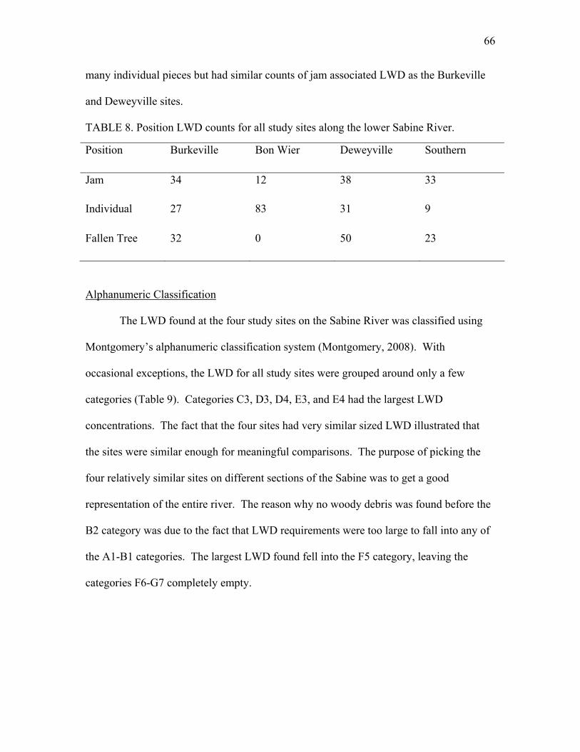
66
m dividual pieces but had similar counts of jam associated LWD as the Burkeville
and Deweyville sites.
TABLE 8. Position LWD counts for all study sites along the lower Sabine River.
Position Burkeville Bon Wier Deweyville Southern
any in
Jam 34 12 38 33
Individual 27 83 31 9
50 23 Fallen Tree 32 0
Alphanumeric Classification
The LW our study sites on the Sabine River was classified using
ery’s alpha c class tion system (Montgomery, 2008). With
occasional excep WD for all study sites were grouped around only a few
ategories C3, D3, D4, E3, and E4 had the largest LWD
concentrations. The fact that the four site ated that
the site e
he
of
D found at the f
Montgom numeri ifica
tions, the L
categories (Table 9). C
s had very similar sized LWD illustr
s were similar enough for meaningful comparisons. The purpose of picking th
four relatively similar sites on different sections of the Sabine was to get a good
representation of the entire river. The reason why no woody debris was found before t
B2 category was due to the fact that LWD requirements were too large to fall into any
the A1-B1 categories. The largest LWD found fell into the F5 category, leaving the
categories F6-G7 completely empty.

67
TABLE 9. Montgomery’s Alphanumeric classification system of LWD on the Sabine
Burkeville Bon Wier Deweyville Southern River.
A1 0 0 0 0 A2 0 0 0 0
A4 0 0 0 0
A6 0 0 0 0 A7 B1
A3 0 0 0 0
A5 0 0 0 0
0 0 0 0 0 0 0 0
B B3
B5 0 0 0 0
B7 0 0 0 0
C2 1 3 3 6 10
C4 1 2 0 2 C5 0 0 0 0
0 0 D1 0 0 D2 0
32 40 32 23 16 6 4 5 1 0 0 0 0 0 0 0
0 0 0 E
2 0 0 0 11 2 2 0
B4 0 0 0 0
B6 0 0 0 0
C1 0 0 0 0
C3 71 16 9
C6 0 0 0 0 C7 0 0
0 4
0 8 9
D3 D4 D5 D6 D7 0
1 0 0 0 0

68
Burkeville Bon WieTable 9 (cont)
r Deweyville Southern E2 1 0 3 0 EE4 17 4 13 13
E6 0 0 0 0
F1 0 0 0 0
F3 0 0 2 0
F5 1 0 0 0
F7 0 0 0 0
G2 0 0 0 0
G4 0 0 0 0
G6 0 0 0 0
3 6 11 16 7
E5 5 0 0 0
E7 0 0 0 0
F2 0 0 0 0
F4 0 1 0 0
F6 0 0 0 0
G1 0 0 0 0
G3 0 0 0 0
G5 0 0 0 0
G7 0 0 0 0 1. Indicates large amount of LWD found in that category.
Unknowns
For each of the four sample sites, with the exception of origin at Burkeville, three
of the categories had a numerous amount of unknowns (Table 10). Species, potential
source, and origin were all difficult to determine in the field. Out of the 119 LWD
samples found at the Deweyville site, 86 were labeled as unknown with the remaining 33
being identified as a mixture of pine and hardwoods. For the potential source category,
83 were called unknowns, 15 were found to be from cutbanks, 7 from windsnaps, and 14
from windthrows. Sixty-five LWD had origins labeled as unknown while 52 were local
and 2 were possibly from upstream. Out of the 95 LWD sampled at Bon Wier, 45
species were unable to be identified. Potential source had 38 unknowns, 43 cutbanks, 10
windthrows, and 4 windsnaps. The origin category had 25 unknowns, 62 locals, and 8

69
were found to be from upstream. Besides the origin category that only had 6 unknowns,
the Burkeville site was fairly similar to others. Out of the 93 LWD sampled, 64 species
ere found to be unknown. Potential source had 52 unknowns, 41 cutbanks, and 0
windsnaps. The origin category had 6 unknowns, 42 locals, and 45 pieces
ite had the least amount of LWD sa findin
ies were fou be unk . For the ial sou
ere found to b own, row had , and
18
from upstream.
TAB d when sampling.
w
windthrows or
found from upstream. The southern s mpled g
67 logs. Out of those 67, 30 spec nd to nown potent rce
category 41 pieces of LWD w e unkn windth 24 logs
windsnap and cut both had 1. The origins category had 24 unknowns, 25 locals, and
logs were found to come
LE 10. Counts of “unknowns” in several categories that could not be determine
Unknowns Burkeville Bon Wier Deweyville Southern
Species 64 45 86 30
Potential Source 52 38 83
Origin 6 25 65
41
24
Total Counts 93 95 119 67
Degree of decay was significantly (p=0.0034) different between the four
locations. Excess LWD in the degree of decay class 4 at the Southern site was
significantly (χ2=9.17, p=0.1349) different than degree of decay in the other classes at the
Sabine contained more decayed LWD (Table 5). Based on the Chi-Square test all four
study sites were not uniformly distributed in the degree of decay category (Table 12).
Statistical Tests Results
remaining three sites (Table A25). This implied that more southerly locations along the

70
Also, LWD pieces that were locked in jams were the ones that were the most decayed
because of their longer residence times. Furthermore, the position of LWD was
significantly (p<0.0001) different between sites. At the Southern site, half the LWD was
located in jams, which was significantly (χ2=10.77, p=0.0418) greater than the other sites
ables 8 and A28). This further supported the observation that more decayed LWD was
located in jams. It would take a large, powerful flood to move some of the jams that were
found on the Sabine, but after a while the LWD in a jam would begin to decay and break
up into smaller pieces, thus breaking up the jam. Burkeville and Deweyville sites
returned a uniformed distribution for the position category (Table 12).
Branch presence on LWD was not significantly (p=0.4354) different between the
sites (Table A30). The presence of branches on the LWD would be expected to influence
the way it interacts within the river system. The interaction between the position of the
LWD and the presence of branches could be due to the branches catching a lot more
debris than a log would catch without branches. The more debris that gets caught, the
bigger the jam becomes and the cycle continues. Based on this conclusion it would be
expected to find more LWD within a jam to have branches, but what was found was that
most pieces within a jam do not have branches. This was due to the fact that when a
piece of wood was decaying, the first thing to fall off was the bark and the branches;
therefore, wood that was stuck in a jam for a long period of time lost its branches.
Branches helped to cause the jam in the first place but eventually get broken off by the
decaying process.
Another aspect of the degree of decay of LWD is the presence of branches. The
lack of statistical significance was unexpected since branch presence was used to help
(T
71
define the degree of decay. LWD was found mostly in the third through fifth categor
of degree of decay (Table 5), which represented pieces wi
ies
th few if any branches. Most
WD w s,
LWD
y.
at
ille site had 62 pieces with a root
e
hat more root
wads were still attached to the LWD. The reason that root wads do not decay as fast as
L as found in the third category at the Burkeville, Bon Wier, and Deweyville site
while the fourth category contained the most LWD at the Southern site. Had more
been found in the first or second categories, then branch presence may have been
significantly different between sites.
The stage contact of LWD was significantly (p<0.0001) different (Table A27).
Where the LWD was at within the bank channel had an influence on its degree of decay.
Most of the LWD were found in the first category, or the low flow contact zone (Table
7). In this zone the pieces would almost always be touched, battered, and decayed by the
flowing water of the Sabine. Due to the constant flow of water it was found that most
pieces of the LWD would be further along in the decaying process. Like previously
mentioned, at all four study sites there was more LWD in the later stages of deca
Root wad presence on LWD was significantly (p<0.0001) different (Table A31).
Again, the degree of decay category showed that the third category had the most pieces
the Burkeville, Bon Wier, and Deweyville sites. The Burkeville site had 53 pieces that
contained a root wad while only 24 pieces did not. The Bon Wier site had 33 pieces that
contained a root wad and 13 that did not, the Deweyv
wad and 41 without, and the Southern site had 20 pieces with a root wad and 46 without.
It would be expected that as the LWD decayed, the root wad would decay with it,
meaning the more pieces found that were heavily decayed then fewer root wads would b
found. But at the Burkeville, Bon Wier, and Deweyville sites it was found t

72
branches and bark was due to the cell structure of root wads. The cells of the root wads
were impregnated with wax which kept them much more water resistant than other parts
of the LWD. The water resistances of the roots are what keep them from decaying at th
same rate as the branches, thus keeping them attached to the LWD for longer periods
time. The presence of a root wad also confirmed that the tree entered the river by either
bank erosion or windthrow because both of these ways will kept the root wad attached. If
a tree enters the river via windsnap then t
e
of
he roots will most likely still be in the ground.
nk
tained more root wads than not. The Deweyville site had a more
uniform distribution for its source category; it had 15 pieces from a cutbank, 14 from a
indthrow, and 7 from a windsnap. Although it was slightly different than either
Burkeville or Bon Wier, its root wad distribution was still consistent with the other two
sites. The Southern site was different in that it had a majority of its pieces coming from
windthrow, but it was unusual in that it had more LWD pieces that did not contain a root
wad. This could be explained by noticing that more of its pieces were in advanced stages
of decay, which means that the root wad would start to decay by the fourth category of
decay.
The origin of LWD was significantly (p<0.0001) different. Due to Burkeville’s
close proximity to the reservoir it would be expected that not a lot of wood would come
from upstream, that most wood would be from the local area. LWD in the upstream class
at the Burkeville site was significantly (χ =15.91, p=0.0248) different than upstream
All of the LWD that could be identified from the Burkeville site were found to come
from a cutbank, meaning the roots were still attached. The Bon Wier site was similar to
the Burkeville site in that it had most of pieces being identified as coming from a cutba
source and it also con
w
2
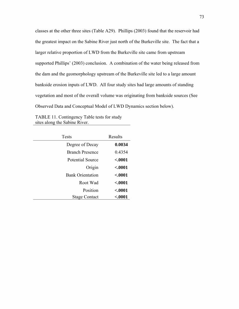
73
classes at the other three sites (Table A29). Phillips (2003) found that the reservoir had
the greatest impact on the Sabine River just north of th
e Burkeville site. The fact that a
roportion of LWD from the Burkeville site came from upstream
the dam and t e pst Bu s a large a
bankside erosion inputs of LWD. All four study sites a ts of stand
vegetation and most of the overall volume riginating from b ide sourc
Observed Data and Conceptual Model of L Dynam sectio w).
TABLE 11. C ntingency Tab sts for stusites along the Sabine River.
larger relative p
supported Phillips’ (2003) conclusion. A combination of the water being released from
h geomorphology u ream of the rkeville ite led to mount
had l rge amoun ing
was o anks es (See
WD ics n belo
o le te dy
Tests Resu
Degree of Decay 0.0034
lts
Branch Presence 4Potential Source <.0001
Origin <.0001Bank Orientation <.0001
n <.0001tac .0001
0.435
Root Wad <.0001Positio
Stage Con t <
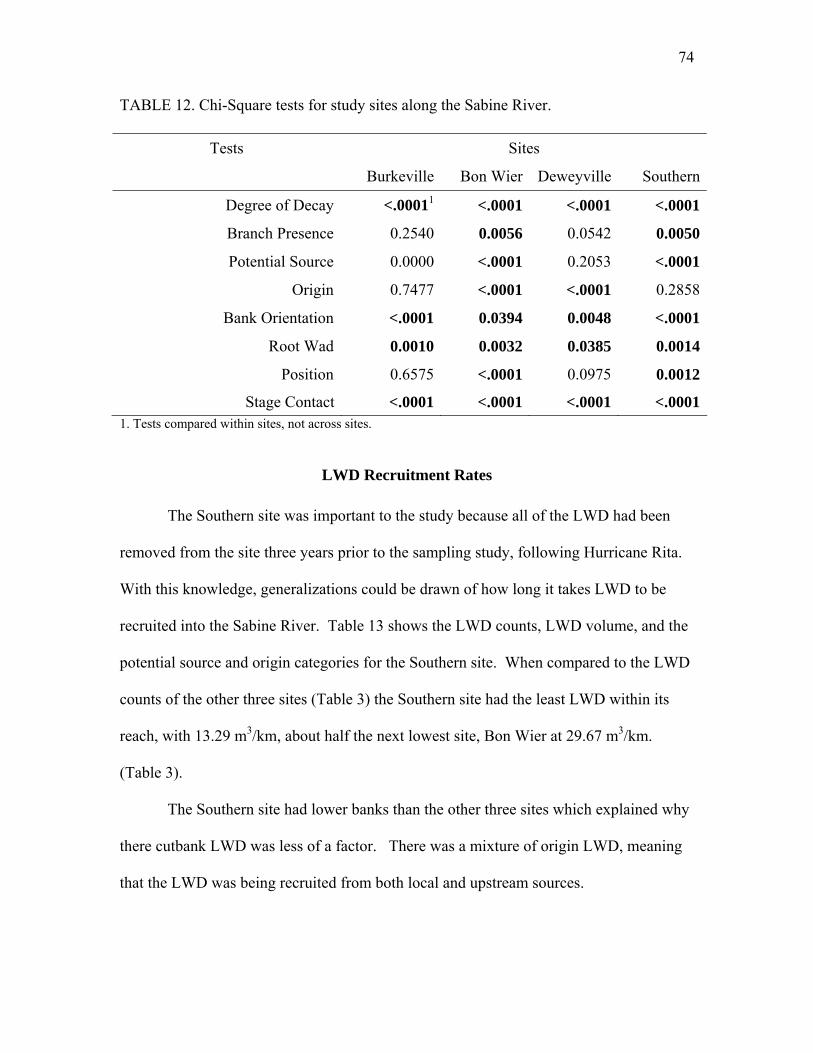
74
TABLE 12. Chi-Square tests for study sites along the Sabine River.
Sites Tests
Burkev Wie yville n
Degree of Decay <.00011 .000
ille Bon r Dewe Souther
< 1 <.0001 <.0001
Branch Presence 540 0056 .0 0
Potential Source 000 0001 .2 1
Origin 477 0001 8
Bank Orientation 001 0394
Roo d 010 0032
Position 575 0001 2
Stage Contact 001 0001
0.2 0. 0 542 0.005
0.0 <. 0 053 <.000
0.7 <. <.0001 0.285
<.0 0. 0.0048 <.0001
t Wa 0.0 0. 0.0385 0.0014
0.6 <. 0.0975 0.001
<.0 <. <.0001 <.00011. Tests compared within sites, no oss sites.
WD itment
The Southern site was important to the study because all of the LWD had been
.
With this kno ledge ti D
recruited into the Sabine River. Table 13 shows the L co D volume, and the
potential source and origin categories for the Southern . When pa
counts of the ther three site able 3) outhern s W
reach, with 13.29 m3/km, about half the next lowest site, Bon Wie 9. 3
(Table 3).
The Southern site had lower banks than the other three sites which explained why
there cutbank LWD was less of a factor. There was a D,
that the LW was being rec d from both local and upstream sources.
t acr
L Recru Rates
removed from the site three years prior to the sampling study, following Hurricane Rita
w , generaliza ons could be drawn of how long it takes LW to be
WD unts, LW
site com red to the LWD
o s (T the S ite had the least L D within its
r at 2 67 m /km.
mixture of origin LW meaning
D ruite
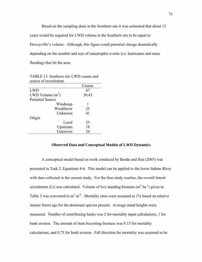
75
TABLE 13. Southern site LWD counts and
Counts
Based on the sampling done at the Southern site it was estimated that about 12
years would be required for LWD volume at the Southern site to be equal to
Deweyville’s volume. Although, this figure could potential change dramatically
depending on the number and size of catastrophic events (i.e. hurricanes and mass
flooding) that hit the area.
source of recruitment.
LWD 67 LWD Volume (m3) 30.43
Windsnap 1
Unknown 41
Local 25
Unknown 24
Potential Source
Windthrow 25
Origin
Upstream 18
Observed Data and Conceptual Models of LWD Dynamics
A conceptual model based on work conduced by Benda and Sias (2003) was
presented in Task 2, Equations 4-6. This model can be applied to the lower Sabine River
with data collected in the current study. For the four study reaches, the overall lateral
recruitment (Li) was calculated. Volume of live standing biomass (m3 ha-1) given in
Table 3 was converted to m3 m-2. Mortality rates were assumed at 1% based on relative
mature forest age for the dominant species present. Average stand heights were
measured. Number of contributing banks was 2 for mortality input calculations, 1 for
bank erosion. The amount of stem becoming biomass was 0.13 for mortality
calculations, and 0.75 for bank erosion. Fall direction for mortality was assumed to be

76
non-preferential, and a value of 0.13 was chosen base on long term averages compiled by
an Sickle and Gregory (1990). Fall direction for bank erosion was based on values
giv r Burkeville
m yr-
1 at Bon Wier and 0.05 m yr at Deweyville and the Southern site. Results are presented
ate differences between the four river
seg ing (85.29 m km ) also had
Deweyville and the Southern sites, the riparian forest volume was much higher with
Tab timates (m km yr ) for the four study reaches on the Lower Sabine River, Texas (Benda and Sias, 2003).
Recruitment (Li)
V
en in Benda and Sias (2003). Mean bank erosion rates were derived fo
from Heitmuller and Greene (2009) at 0.1341 m yr-1, and were estimated to be 0.10
-1
in Table 14.
Lateral recruitment estimates illustr
ments. Burkeville, which has the highest total LWD load 3 -1
the highest recruitment rate and recruitment was dominated by bank erosion. On
much lower bank erosion rates, and mortality recruitment dominated.
le 14. Lateral recruitment budget es 3 -1 -1
Site Mortality Recruitment (Im)
Bank Erosion Recruitment (Ibe)
Total Lateral
Burkeville 1.40 3.52 4.92 Bon Wier 0.95 1.86 2.81
eyville 1.80Dew 1.53 3.33 Southern 1.92 1.79 3.71
These estimates of lateral recruitment can then be com pared with the overall
esti in Task 5, specific estimates are
southeast Texas has one of the highest wood decay rates in the continental United States,
woody debris budget estimate presented in Task 2, Equation 9. To accomplish this, an
mate of woody debris decay is needed. As reported
not available, though decay rates can be between 2 and 7% of live biomass in a forest
floor environment (Spies et al., 1988). Due to warm temperatures and high humidity,

77
so the higher end of this range, 7%, was used for budget calculations. With a 7% deca
, the average decay based residence time for a pie
y
rate ce of LWD would be 14.29 years.
5).
The unknown variables were the volume of woody debris flowing into the reach (Qi), the
volume plain
out of the reach (Lo). For the Burkeville and Deweyville sites, this volume was a net
positive
greater
xpected given the higher rates of bank erosion immediately downstream of Toledo Bend
Reserv
his is also consistent with the lateral recruitment estimates for Burkeville, where
recruitm es higher than recruitment due to mortality (Table
adings due to reservoir interruptions of fluvial LWD at the Burkeville site. Additional
measur 2003)
was observed would be necessary to determine if these LWD reservoir storage effects
extend lle site. At Deweyville, forest mortality recruitment is
wer
gradien may be occurring. For Bon Wier, it
remainder may be transported off site (0.54 m km yr ) as fluvial outflow or floodplain
rs
since th ging operation, with a lateral recruitment estimate of
The total woody debris budget was then calculated from Equation 9 (Table 1
flowing out of the reach (Qo), and the volume being deposited on the flood
, meaning that fluvial transport of wood into the reach is likely occurring at a
rate than fluvial outflow. This value was highest at Burkeville, which is to be
e
oir reported by Phillips (2003) and is also consistent with measured source data.
T
ent due to erosion is 2.5 tim
14). It is unlikely that the Toledo Bend Dam had a significant impact on reducing LWD
lo
ements immediately below the dam in which the scour reported by Phillips (
upstream of the Burkevi
greater than bank erosion, due to the lower gradients at this site. Also, with lo
ts more LWD accumulations from upstream
is estimated that more wood is being recruited than stored in the channel, so the
3 -1 -1
deposition. At the Southern site, LWD accumulation has only occurred for about 3 yea
e post-Hurricane Rita snag

78
10.47 m3 km-1, meaning that the difference of 2.82 m3 km-1 may have come in as fluvia
from further upstream.
l
inflow
ne River TVariabl thern
Table 15. Estimated woody debris storage, decay, and recruitment for the lower Sabi
exas. e Burkeville Bon Wier Deweyville Sou
Total R 3.33 3.71ecruitment (Li, m3 km-1 yr-1) 4.92 2.81Volume Decayed (D, m km yr ) 0.34 0.20 0.23 0.22
3.49Recruit .29 37.29 44.29 49.86
olume Measured (m3 km-1) 85.29 29.67 49.63 13.29N/A
3 -1 -1
Net Recruitment (m3 km-1 yr-1) 4.58 2.61 3.10 ment in 14.29 Yrs (m3 km-1) 69
V (Qi – Qo – Lo) Vol. (m3 km-1 yr-1)a 1.05 -0.54 0.38 a Qi = Ldeposit n site since it was snagged 3 years
rior to measurement.
estimat on, decay, and mortality rates. Future studies will need
o represent a reasonable approximation of LWD dynamics in the lower Sabine River.
One ob is that the riparian forest density and volume
be
etween 11 and 21% of total annual recruitment, with the remainder governed by lateral
recruitm e most
effectiv ect
nd enhance the riparian forest. There does not seem to be much evidence from this
analysi in the
transport limited for sediment, and the same seems to be generally true for LWD. It is
likely t s
WD from fluvial inflow, Qo = LWD from fluvial outflow, Lo = floodplain ion. Estimates are not available for the Souther
p
These budget estimates do have a high degree of uncertainty, particularly for
ed variables like bank erosi
to quantify these variables for more precise budget estimates. However, these numbers
d
vious conclusion from these data
plays a significant role in LWD recruitment. Fluvial dynamics were estimated to
b
ent, which depends mostly on surrounding forest density. Therefore th
e means of enhancing LWD recruitment for the lower Sabine would be to prot
a
s that the Toledo Bend Dam had a significant impact on LWD dynamics
lower Sabine River due to LWD storage. As noted by Phillips (2003), the lower Sabine
is
hat the large volumes of LWD that were historically in the rivers of East Texa

79
were du e
cypress and oak and that centuries of riparian forest degradation and invasive species
spread
Oregon a
135 yea of LWD compared to the Sabine. They
ildfire. The quantity of LWD they found was a direct result from the balance of debris
puts and outputs of the stream system. They reported that the input of LWD was
control
anks, and the ability of the stream to transport LWD downstream. The biggest
contrib
torrents, and stream cleanup after logging. The export of LWD was found to be caused
by the a
physica
ithin the
stream
wanson et al., 1976; Palik et al., 1998; Hedman et al., 1996). Other studies have
shown
ere the major contributors to LWD input (O’Connor and Ziemer, 1989). A study by
Murphy WD was recruited by bank erosion and
e to the large, dense forests composed of relatively decay resistant species lik
resulted in lower maximum potential LWD loadings.
Comparison to Other River Systems
Other studies that have examined LWD have found similar results to the study of
LWD in the Sabine. For example, Swanson et al. (1976) studied LWD on Western
streams and found that a stream flowing through both a 75 year old stand and
r old stand contained similar counts
found the LWD to be an important factor in the stream environment, even after a severe
w
in
led by age and condition of the surrounding forest, the stability and steepness of
b
utors of LWD in their study were blowdowns, extreme discharge events, debris
bility of the stream to float debris downstream, rates of decomposition, and
l breakdown of debris in channels. Like the study of the Sabine, other researchers
have found that many variables contribute to the import and export of LWD w
system and all variables must be considered when looking at the whole picture
(S
that bank erosion, windthrow, logging debris, wind fragmentation, and landslides
w
and Koski (1989) found that most L

80
windthrow. Of the LWD that had identifiable sources, the researchers found that 99
percent
geomorphology, vegetation, and hydrology. Other studies performed showed that
WD input into the stream system, or that landforms controlled a variety of ecosystem
pattern
southwestern Georgia and found that constrained reaches, like sand ridges and terraces,
had the am, while
dies
showed chers like
ridges) et al. (1998) went on to suggest that
o
the area tween the sand
arts of the river were more likely to input LWD and transport it downstream and other
par
mport
and exp ch in several studies. The ability of a stream to move
e
the Sab
came from within 30 meters off the stream bank.
Differences among sites on the Sabine River can be attributed to variations in
geomorphic differences among reaches resulted in different patterns of tree death and
L
s and processes (Swanson et al., 1988). Palik et al. (1998) studied a stream in
highest tree mortality rates which recruited the most LWD into the stre
floodplains and terraces had low tree mortality and low LWD recruitment. Other stu
that large floods were the primary source for LWD recruitment. Resear
Palik et al. (1998) found that most LWD was from constrained stream valleys (i.e. sand
(Golladay and Battle, 2005). Palik
unconstrained reaches, floodplains, could become LWD sinks, where LWD moved int
but did not move any further downstream. The relationship be
ridges and floodplains could become what they call a “source-sink relationship” where
p
ts would more likely keep the LWD it receives.
The transport of LWD downstream was an important function of the LWD i
ort from a given stream rea
a piece of LWD downstream was more of a characteristic of higher order streams, lik
ine (Keller and Swanson, 1979; Lienkaemper and Swanson, 1987).

81
Like the study on the Sabine, O’Connor and Ziemer (1989) found many pieces
that had to be classified as unknown, and they attributed this to the amount of time since
were found to be unknown, they were able to find that 60 percent of the LWD from
he
channe e
LWD v
LWD in 9 transects that were placed along the river. If 9 transects in Benke and Wallace
(1990) the lower
the least amount of standing trees with a total trees ha-1 of
e greatest number of stems, with 52.5 17 trees ha-1. The basal area was rather low, at
14.4 m
l
olume and basal area were lower. (Table 17). This is due to the fact that this site had
more sm nce again most stems
stockin
The Deweyville site had more stems, volume, and basal area than the previous
two site a-1 indicates rather good stocking, and
the trees had fallen and also to the fragmentation of the LWD. Although many pieces
outside of the bank channel came from windthrow. LWD that occurred from within t
l were mostly from bank erosion. The researchers also noted that 27 percent of th
olume was found to be in a jam.
Benke and Wallace (1990) found on the sixth order Ogeechee River 66 pieces of
are equal to 1 meander scar in the current study, then LWD loads in
Sabine were greater.
Bankside Vegetation Inventory
The Burkeville site had
210 and a total volume of 349.9 m3 ha-1 (Table 16). The 15 centimeter diameter class had
th
2 ha-1, indicating that the stand is not fully stocked.
While the Bon Wier site had slightly more stems per hectare (220), the overal
v
aller trees, accounting for less overall volume per stem. O
were in the 15 cm diameter class. A basal area of 11.5 m2 ha-1 indicates rather poor
g for a bottomland hardwood forest.
s (Table 18). The basal area of 18.8 m2 h
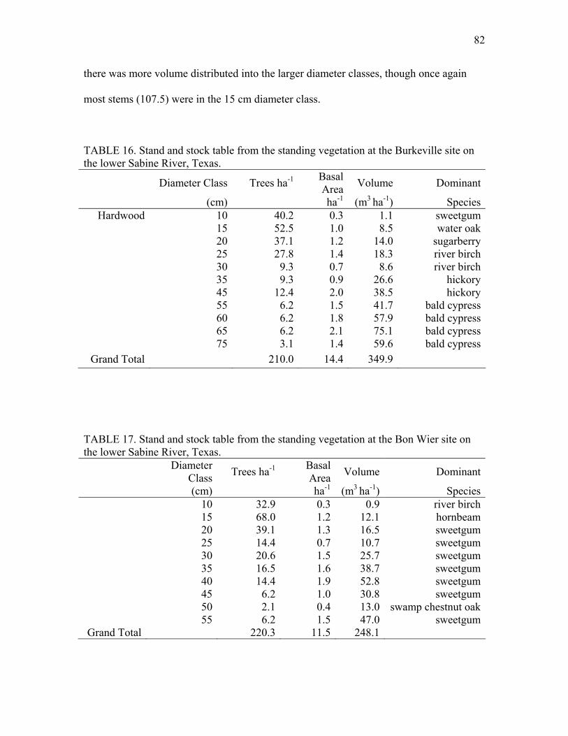
82
there was more volume distributed into the larger diameter classes, though once again
most st
TABLE 16. Stand and stock table from the standing vegetation at the Burkeville site on the lower Sabine River, Texas.
t
ems (107.5) were in the 15 cm diameter class.
Diameter Class Trees ha-1 Basal Area Volume Dominan
(cm) ha-1 (m3 ha-1) SpeciesHardwood 10 40.2 0.3 1.1 sweetgum
15 52.5 1.0 8.5 water 20
oak37.1 1.2 14.0 sugarberry
25 27.8 1.4 18.3 river birch
ryoryess
s5 6.2 2.1 75.1 bald cypress
75 3.1 1.4 59.6 bald cypressGrand Total 210.0 14.4 349.9
30 9.3 0.7 8.6 river birch 35 9.3 0.9 26.6 hicko 45 12.4 2.0 38.5 hick 55 6.2 1.5 41.7 bald cypr 60 6.2 1.8 57.9 bald cypres 6
TABLE 17. Stand and stock table from the standing vegetation at the Bon Wier site on the lower Sabine River, Texas.
Diameter Class Trees ha-1 Basal
Area Volume Dominant
(cm) ha-1 (m3 ha-1) Species 10 32.9 0.3 0.9 river birch 15 68.0 1.2 12.1 hornbeam 20 39.1 1.3 16.5 sweetgum 25 14.4 0.7 10.7 sweetgum 30 20.6 1.5 25.7 sweetgum 35 16.5 1.6 38.7 sweetgum 40 14.4 1.9 52.8 sweetgum 45 6.2 1.0 30.8 sweetgum 50 2.1 0.4 13.0 swamp chestnut oak 55 6.2 1.5 47.0 sweetgum
Grand Total 220.3 11.5 248.1

83
TAB E 18. on
e lower Sabine River, Texas.
Cla me Dominant
L Stand and stock table from the standing vegetation at the Deweyville site th
Diameter Trees ha-1 Basal Area Voluss (cm) h (m Species 10 .2 0 Chinese Tallow
a-1 3 ha-1)43 .3 1.1
15 .5 1 Chinese Tallow 20 40.8 1 Chinese Tallow 25 46.9 2 hickory 30 38.3 2 hickory 35 29.7 2 Chinese Tallow 40 13.6 1 black willow 45 12.4 2 sweet gum 50 4.9 water oak 55 6.2 1 water oak 60 1.2 0 green ash 65 1.2 0 sweet gum 75 1.2 0 water oak
Grand Total 347.2 18
107 .9 21.5.3 20.9.3 36.1.7 53.8.9 56.2.7 43.9.0 58.0
1.0 21.6.5 44.9.3 14.9.4 13.6.5 20.6
.8 407.1
TABLE 19. Stand and stock table from the standing vegetation at the Southern site on the lower Sabine River
D a-1 B l A V Dominant
, Texas. iameter Trees hClass asa rea olume
( h (m Species 10 57.7 0 Chinese Tallow
cm) a-1 3 ha-1).5 1.6
15 45.3 0 Chinese Tallow 20 37.1 Chinese Tallow 25 41.2 2 hickory 30 .9 2 hickory 35 14.4 Chinese Tallow 40 8.2 1 black willow 45 4.1 0 sweet gum 50 4.1 water oak 55 10.3 2 water oak 60 2.1 green ash 65 2.1 0 sweet gum 75 8.2 water oak
Grand Total 6.2
.8 8.81.2 15.6.1 30.9
30 .3 28.71.4 38.0.1 28.4.7 18.5
0.8 22.1.5 69.5
0.6 15.8.7 19.1
3.3 93.0 2.8 86.3

84
The Southern site had best stocked forest, with an overall basal area of 20.8 m2
ha-1. It also had the most vo d stems per hectare (Table 19). An ANOVA was
conducted on total volume and no significant differences between sites was observed
(p=0.4118). This lack of statistical significance can in part be attributed to the large
amount of variation observ individual ts in stand. Riverside volumes
tend to be rather heterogeneous overall. One co usi t can ached is that recent
hurricanes have not resulted in significant fores se sit er to the coast
when compared to the sites further upriver, thou Hu e Ri articular did result
in significant LWD contributions to the river (Phillips and Park, 2009). Another
important observation is t of Chin tal e in the two southernmost
sites, particularly in the sm ter classe his indi at regeneration of
native species is being inh is e dominate the
future forest at these sites. wood of Chinese tallow is less durable than
species like oak and cypress, and this may alter future average residence times of LWD
due to decay.
lume an
ed among plo each
ncl on tha be re
t los s in the es clos
gh rrican ta in p
he dominance ese low tre
a eller diam s. T may cate th
ibited, and that th xotic invasive tree will
In general,

85
LITERATURE CITED
Abbe, T.A. and Montgomery 996. Larg ody am el hydraulics, and habitat formation i Regulated Rivers . Ma
Abbe, T.B., A.P. Brooks R. 2003. Wood in river rehabilitation and
management. A ocie ympo , p. 1 Andrus, C.W., Long, B.A., Froehlich, H.A. 198 oody debris and its contribution to pool
formation in a coasta 0 years af loggin nadi rnal of Fisheries and Aquatic Science -2086.
Benda, L.E. and Sias, J.C. 2003. A quantitative ework for evaluating the mass balance of
in-stream organic de Systems Institute. 2-12. Benke, A.C. 1984. Secondary production of aquatic insects. Pages 289-322 in V.H. Resh and
D.M. Rosenberg, eds of aquati sects. er, N ork, NY. Benke, A.C., Henry, R.L., D.M., ter, R 84. I nce of snag habitat
for animal production in southeastern streams. Fisheries, Vol. 10, No. 5. Benke, A.C. and J.B. W d dyn cs in Coastal Plain blackwater streams.
Can. J. Fish. Aq Beven, K., Gilman, K., N Flow flow ng in d channel
networks. Hydro 4(3) 3-325 Bilby, R.E. 1984. Post-logg l of woo ebris s stre annel stability.
Journal of Forestry. 82: 609-613. Bilby, R.E. and Likens, G.E ortance rganic is da the structure and
function of stream ec Ecology 61: 1107-1113. Bilby, R.E., Heffner, J., Fransen, B., Ward, J., Bisson, P. 1999. Effects of submergence on
deterioration of wood from five species ees us r hab hancement projects. North Am. anage. 19 7-695
Blinn, C.R. and Kilgore ian m geme ctice or. 99 (4), 11-17. Bragg, D.C. and Kershner, J.L. 1999. Coarse woody debris in riparian zones. J. For. 97 (4),
30-35. Braudrick, C.A. and Grant, G.E. 2000. When do logs mov ers? Resources Res. 36,
571-583.
, D.R., 1 e wo d s jebri s, channn large rivers. : Res nage. 12.
, Montgomery, D.merican Fisheries S ty S sium -25.
8. Wl s 5
s. 45: 2080tream ter g. Ca an Jou
frambris. Earth
. Ecology c in Praeg ew Y
III, Gillespie, Hun .J. 19 mporta
allace. 1990. Woo amiuat. Sci. 47: 92-99.
ewson, M. 1979. and routi uplanlogical Sci. Bull., 2 , 30 .
ing remova dy d affect am ch
. p 1980. Im.
of o debr ms in osystems
of tr ed fo itat enJ. Fish. M , 68 .
, M.A. 2001. Ripar ana nt pra s. J. F
e riv Water

86
Clark, A. III, Souter, R.A. 1996. Stem cubic oot volume tables for tree species in the Deep South Area. Res. Pap. SE-293. Ashville, NC: U.S. Department of Agriculture, Forest Service, Southern Research Station. 131.
Couch, C.A. and Meye evelop t and
biofilms in a blackwater river. Freshwater Biology. 27: 43-51.
Cudney, M.D. and Wa 0. Life les, m istrib and production dynamics of six species of net-spinning caddis in a l outheastern (U.S.A.) rive : 169 .
Dolloff, C.A. 1993. Large woody debris, fish habitat, and historical land use. In J.W. McMinn and D.A , Jr. (eds iodive and woody debris in southern forests, proceedings of the workshop on coarse woody debris in southern forests: effects in ity, USDA For. Ser. Gen. Tech. Rep. SE-94, pp. 120-138.
Ehrmann, T.P. and Lamb 1992. H aulic and particulate matter retention in
a 3rd order In rnal o e Nor eric thological Society, 11, 341-349.
Einstein, H.A. and Banks, R.B. 1950. Fluid resistance of composite roughness. Eos
Trans. AGU, 31, 603-610.
Evans, B.F., Townsend, C.R., Crowl, T.A. 1993. New Zealand Journal of Marine and Freshwater Rese 27-239.
Fausch, K.D. and No . Lar oody is an onid habitat in a
small coastal British Columbia streaAquatic Sciences 93.
Gippel, C.J. 1995. Envir ydraulic large woody debris in streams and rivers. J. Env. Eng., 388
Gippel, C.J., O’Neill, I.C on, B.L. 1 . The ulic of snag
management, Ctr r. Appl. H ro., D Civ Agric. Engrg., Univ. of Melbourne, Parkville, Australia.
Golladay, S.W and Battle, J. 2005. Wood debris recru t fro ering riparian
landforms in a Gulf Coastal Plain stream: TheNewton, GA. 1-3.
Goodburn, J.M. and Lor 1998. Ca tree oars dy debris in old-
growth and managed northern hardwood forests in Wisconsin and Michigan. Can. J. For. Res. 29, 4
-f
r, . DJ.L. 1992 men composition of the epixylic
llace, J.B. 198 cyc icrod ution flies arge s
r. Holarct. Ecol. 3 -182
. Crossley .), B rsity coarse
biodivers
erti, G.A. ydrdiana stream. Jou f th th Am an Ben
arch. 27: 2
rthcote, T.G. 1992 ge w debr d salmm. Canadian Journal of Fisheries and
49: 682-6
onmental h s of-399.
., Finlays 992 hydra basis . For Envi yd ept. of . And
itmen m diff Role of Floods. J. Eco. Res. Cen.
i .mer, C.G vity s and c e woo
27-438.

87
Haga, H. Kumagai, T. Otsuki, K. Ogawa, S. 2002. Transport and retention of coarse woody debris in mountain streams: An in situ field experiment of log transport and a field survey of coarse woody debris distribution. Water Resources Research 38:1-1-1
Harmon, M.E., Franklin, nson, F.J. llins, egor ., Lattin, J.D.,
Anderson, N.H., Cline, S.P., Aumen, N.G., Sedell, J.R., Lienkaemper, G.W., Cromack, K., Jr., Cummins, K.W. 1986. Ecology of coarse woody debris in temperature col. 15, 133-302.
Harmon, M.E. and Hua, C., 1991. Coarse w y deb ami wo old-growth
ecosystems. BioS : 604-610 Hedman, C.W., Van Lea ank, W. 996. am l oody debris
loading and stag n the ern Appalachian Mountains. C , 121 227.
Heitmuller, F.R. and Gre 2009. H ric ch adju and estimates of
selected hydrau he lowe bine R and Brazos River Basins, Texas and Louisiana. U.S. Geological ey S ic Investigations Report 2009-51
Hey, R.D. 1988. Bar fo in grav ed riv 114: 1498-
1508. Hooke, J.M., 1980. Magnitude and distribut of rat iver rosion. Earth Surf.
Process. Landforms Huryn, A.D. and Wallace, J.B. 1987. Local geomorphology as a determinant of
macrofaunal production in a mountain stream. Ecology. 68: 1932-1942. Huston, M.A. 1993. Models and management implications of coarse woody debris
impacts on biodiversity. In J.W. McMinn and D.A. Crossley Jr. (eds.), Biodiversity and coarse woody debris in southern forests, proceedings of the workshop on coarse woody debris in southern forests: effects on biodiversity. USDA For. Ser. Gen. Tech. Rep. SE-94. pp 139-143.
Hyatt, T.L. and Naiman, R.J. 2001. The residence time of large woody debris in the
Queets River, Washington, USA. Ecological Applications 11:191-202. Keller, E. A. and Swanson, F.J. 1979. Effects of large organic material on channel from
and fluvial processes. Earth Surface Processes. 4, 361-380. Keller, E.A and Tally, T. 1979. Effects of large organic debris on channel form and
fluvial processes in the costal redwood environment. – In: Rhodes D.D. and Williams P.G. (eds.) Adjustment of the Fluvial System. Proceedings of the Tenth
-16.
J.F wa., S , So P., Gr y, S.V
ecosystems. Adv. E Res.
ood ris dyn cs in tcience, 41 .
r, D.H., Sw T. 1 In-stre arge wriparian forest seral
an. s. 26e associations i south
J. For. Re 8-1
ene, L.E. isto annel stmentlic values in t r Sa iver Lower
Surv cientif74, 143 p.
rm resistance el-b ers, J. Hydraul. Eng.,
ion es of r bank e 5: 143-157.

88
Annual Geomorphology Symposium. pp 169-197. State Univ. of New York, Bingham
Lienkaemper, G.W., Swanson, F.J., 1987. Dynamics of large woody debris in streams in old growth Douglas fir forests. Can For. R 7, 150
Likens, G.E., Bilby, R.E., 1982. Developm maintenance, and role of organic-debris
dams in New England streams. In: Swanston, D.N kshop o dime gets a ting in forested drainage basi 1. USD orest e, Por OR, pp. 122-128.
MacDonald, A., Keller, E. A. and Talley, T. 1982. T ole of
stream channels draining Redwood forests northwestern California. In Harden, D.K. Marran, D.C. and MacDonald, A. (eds) Late Cenzoic history and forest geomorphology of Humbold Co. California, acific Cell fieldtrip guidebook, 226-245.
Magna, M., Kirchner tress pa oning eams by large woody debris.
Water Resources Research, Vol. 36, No. 8, Pages 2373-23779, August 2000. Malanson, G.P., 1993. ndscapes mbridge University Press, Cambridge. Manner, R.B. and Doy 008. A m hanist del of debris jam
evolution and i n to woo ased r ation a nagement. River Research Appli 1104-112
Marzolf, G.R. 1978. T agging on stream ecosystems.
Fish and Wildlife Service, U.S. Department of the Interior, Washington, D.C. 30 pp.
Maser, C.M., Cline, S.P k, K., Jr., Trappe, J.M., Hansen, E. 1988. What we know about large trees that fall to the forest floor. In C.M. Maser, R.F. Tarrant, J.M. Trappe, J.F. Franklin (eds.), F the fo the strees. USDA For. Ser. Gen. Tech. Rep. PNW pp 25
McClure, J.M., Kolka, R.K., White, A. 2004. Effect of forest harvesting best
management practices on coarse woody debr ributi tream and riparian zones in three Appalachian watersheds. Wate , and llution: Focus. 4: 245-261.
Minshall, G.M., Peterson, R.C., Cummins,
1983. Interbio n of str ecosystem dynam . 53: 1-25.
Montgomery, D.R. 2008. A sim alphanu ric cla ation o d debris size and
shape. Stream Notes
ton.
. J. es. 1 -156.
ent,Swanson, F.J., Janda, R.J., Dunne, T.,
. (Eds.), Wor n se nt bud nd rouns. PNW—14 A F Servic tland,
he r large organic debris in
Friends of the Pleistocene, P
, J.W. 2000. S rtiti in str
Riparian la . Ca
le, M.W. 2 ec ic mo woodyts applicatio d-b estor nd macations 24: 3.
he potential effects of clearing and sn
., Cormac
rom rest to ea: A story of fallen -229. -47.
is dist on in sr, Air Soil Po
K.W., Bott, J.R., Cushing, C.E., Vannote, R.I. me compariso eam ics. Ecol. Monogr
ple me ssific f woo. October 2008.

89
Muller, R.N., Liu, Y. 1991. Coarse woody debris in wth us forest on the
Cumberland Pla theastern ucky . J. For . 21, 1567-1572.
Murphy, M.L., Koski, K.V. 1989. Input and depletion of woody debris in Alaska streams and implementation for streamside gem orth A Fish. Manage. 9, 427-436.
Mutz, M. 2000. Influen dy debri flow ns ad el morphology in a
low energy, sand-bed stream reach. ernat. ydro 07-121. Nakamura, F., Swanson, F.J. 1993. Effects oarse y deb morphology and
sediment storag ntain stre in western Oregon. Earth Surf. Process. Landforms 1
Nunnally, N.R. 1978 ation: lterna o chan tion,” Environmental Management, Vol. 2, No. 5, Sept., 1978, pp. 403-410.
Nunnally, N.R., and K 9. “Use luvial sses to mize adverse
effects on stre ation,” R rt No ate urces Research Institute of the University of North Carolina, Raleigh, N.C., July, 1979.
O’Connor, M.D., Ziem 89. Coar oody ecolo a second-growth
Sequoia semper st stream S. De ent of ulture For. Ser. Gen. Tech. Rep
Palik, B., Golladay, S.W., Goebel, P.C., Ta r, B.W 8. Geo hic variation in
riparian tree am coarse woody debris recruitment from record flooding in a Coastal Plain stream. scienc ): 551
Phillips, J.D. 2003. Toledo Bend reservoir and geom c resp the lower Sabine
River. River R : 137-1 Phillips, J.D. and L. Park. 2009. Forest blown impacts of Hurricane Rita on fluvial
systems. Earth S ses and dform 1069- Putz, F.E., Sharitz, ane d ge to old-growth forest in Congaree
Swamp National Monument, South Carolina, U.S.A. Ca Journal of Forest Research. 21: 1765-1770.
Reinhardt, R.D. M. McKenney-Easterling, M.M. Brinson, J.M. Masina-Rubbo, R.P.
Brooks, D.F. W ’Brien, . Hite .K. A ng. 2009. Canopy compo orest stru e prov estoration targets for low-order riparian ecosyst oration E gy 17:51-59.
old-gro deciduoteau, Sou Kent . Can . Res
mana ent. N m. J.
ces of woo s on patter channInt Rev. H biol., 1
of c wood ris on e of a mou am
8, 43-61.
. “Stream renov an a tive t neliza
eller, E. 197 of f proce miniam channeliz epo . 144, W r Reso
er, R.R. 19 se w debris gy invirens fore. P
. U. partm AgricSW-110. 1989.
ylo . 199 morp mortality and stre
Eco e. 5(4 -560.
orphi onse ines. Applic. 19 59.
urface Proces Lan s, 34: 1081.
R.R. 1991. Hurric amanadian
igham, D. O J.T , and B rmstros fition and ctur ide rems. Rest colo

90
Robison, E.G., Beschta, R.L. 1990. Coarse woody debris and channel morphology interactions for undisturbed stream outh askaProcesses Landforms , 149-156
Seo, J.I. and F. Nakam Scale-de dent c ls upo luvial export of
large wood from hments. th Sur Proce d Landforms 34:786-800.
Sharitz, R.R., Vaitkus, M.R., Cook, A.E., 1992. Hurricane dama n old-growth
floodplain forest in the southeast. In: Brissette, John C., ed. Proceedings of the Seventh Bienni Silvicul l Rese onfe 1992 November 17-19; Mobile, ech. Rep -93. N rleans U.S. Department of Agriculture, Fo e, Southe orest iment Station: 203-210.
Shields, F.D., Gippel, C Prediction
resistance. J. Hydraul. Eng. 121, 341-354.
Shields, F.D. and Nunnally, N.R. 1984. Environmental aspects of clearing and snagging. J. of Env. Eng . 110, N , Febr 1984. 54.
Simons, D.B., Li, 1982. Engineering analy tems, Fort Collins, Colo.,
1982. Smith, R.D., Sidle, R.C., Porter, P.E., Noel . 199 ects o rimental removal
of woody debris on the channel mo logy of a forest, gravel-bed stream. J. Hydrol. 152
Smock, L.A., Gladden, enberg, J acroinvertebrate production
in a southeastern United States blackwater stream. Ecology. 66: 1491-1503. Smock, L.A., Metzler en J.E.. 9. Rol ebris n the structure and
functioning of low-gradient headwa stream ology 64-775. Spies, T.A., Franklin, , T.B., 1988. Coarse woody debris in Douglas-fir
forests of wes nd Washington. Ecology 696, 1689-1702. Swanson, F.J., Kratz, T.K., Caine, N., Woodmansee, R.G., 1988. Landform effects on
ecosystem patte ocesses. B cienc 92-98 Swanson, F.J., Lienkaemper, G.W., Sedell, ., 197 tory, al effects, and
management im of large o nic de west egon streams. Pacific Northwest Forest and Range Experim ation epartment of Agriculture, Portland Oregon.
Thibodeaux, L.J. and Boyle, J.D. 1987. Bedform-generated convective transport in
bottom sediment. Nature, 325, 341-343.
s in s east Al . USA, Earth Surf. . 15 .
ura. 2009. pen ontro n the f river catc Ear face sses an
ge to a
al Southern tura arch C rence; AL. Gen T . S0 ew O , LA: rest Servic rn F Exper
.J. 1995. of effects of woody debris removal on flow
ineering, Vol o. 1 uary, 152-1
sis of fluvial sys
, J.R 3. Eff f experpho
, 153-178.
J.E., Riek .L. 1992. Lotic m
G.M., Gladd 198 e of d dams iter s. Ec . 70: 7
J.F., Thomastern Oregon a
rns and pr ioS e. 38: .
J.R 6. His physicplications rga bris in ern Or
ent St U.S. D
91
Thorp, J.H.; McEwan, E.M., Flynn, M.F. 1985. Inv te c erged
Wood in a cypress-tupelo swamp and blackwater stream.Naturalist.
Trimble, S.W. 1997 erosio nd change resulting from riparian -forests.
Geology. 25, 4
Van Sickle, J., Gregory 0. Model inputs rge w ebris to streams from falling trees. Can J. For. Res. 20, 1593-1601.
Wallace, J.B., Benke, A.C. 1984. Quantification of w abita btropical Coastal
Plain streams. rnal of eries quatic ces. 41: 1643-1652.
Wallace, J. B., Grubaugh, J. W iles, M. 993. ces o se woody debris on
stream habitats ebrate bio ersity cMin ., and Crossley, D.A., Jr., eds. Biodiversity and Coarse Woody Debris in Southern Streams: Proceedings of the Woo ebris i thern Forests: Effects on Biodiversity. Athens, GA, USDA st ServStation, Ashville,
ertebra olonization of subm American Midland
113:56-68.
. Stream channel n a67-469.
, S.V., 199 ing of la oody d
ood h t in su Canadian Jou Fish and A Scien
., W R. 1 Influen f coarand invert div . In: M n, J.W
Workshop on Coarse dy D n Sou Fore ice Southern Research
NC.

92
APPENDIX A – DATA AND ST TICAL ANALYSIS
TA ille bank standin me. DBH ht V
ATIS
BLE A1. Burkev side g voluSpecies Heig olume
(cm) y 10 0
(m) (m3) American holl 6.1 0.020
American hornbeam 10 am 10 0
ry 10 ry 10
10 etgum 10
m 10 3 m 10 n 10 k 10 7 k 10 k 10
15 7 ry 15
h 15
ry 15 rberry 15
15 7 k 15 9
Am hornbeam 15 7 rnbeam 15 nbeam 15 m 15 4 ow 15 15 h 15 k 15 7
ak 15 am 20
20 2 20 ry 20 2
20 7 h 20
ry 20 2 ry 20 ry 20 9 m 20 7 k 20
Sycamore 25 13.72 0.198 Water oak 25 6.10 0.133
4.57 0.020 American hornbe 6.1 0.020
Sugarber 6.10 0.020 Sugarber 6.10 0.020 Sweetgum 4.57 0.020 Swe 9.14 0.020 Sweetgu 8.5 0.020 Sweetgu 7.62 0.020 Unknow 2.44 0.020 Water oa 10.6 0.020 Water oa 9.14 0.020
Willow oa 7.62 0.020 Elm 4.5 0.020
Hicko 9.14 0.020 Oak 15 4.57 0.020
River birc 4.57 0.020 Sugarber 7.62 0.020 Suga 7.62 0.020 Water oak 10.6 0.025 Water oa 12.1 0.028
erican 10.6 0.065 Am hoAmerican hor
erican 3.05 0.051 6.10 0.051
Blackgu 9.1 0.051 Blackwill
Hickory9.14 0.051 6.10 0.051
River bircWater oa
7.6210.6
0.051 0.065
Water o 6.10 0.051 American hornbe
ress 4.57 0.076
Bald cyp 13.74
0.113 Hickory 9.1 0.076
Sugarber 7.6 0.076 Unknown 20 4.88 0.076 Hickory
rc10.6 0.125
River bi 3.05 0.105 Sugarber 13.7 0.153 Sugarber 7.62 0.105 Sugarber 12.1 0.139 Sweetgu 10.6 0.125 Water oa 7.62 0.105

93
TABL inued).
ht V E A1. (Cont
Species DBH Heig olume (cm) )
25 2 (m (m3)
Elm 13.7 0.246 River birch 25 9
h 25 2 h 25
wn 25 k 25 k 25 7 k 30 7 ss 30
irch 30 9 35 4
35 4 k 35 6 ory 45 6
ory 45 9 k 45 2
press 55 6 55 4
ress 60 8 60 1 ss 65 8 ss 65 8
ess 75 6
12.1 0.224 River birc
irc7.6 0.167
River b 7.62 0.167 Unkno 8.84 0.167 Water oa 4.57 0.167 Water oa 10.6 0.204 Water oa
pre10.6 0.275
Bald cy 4.57 0.328 River b 12.1 0.328 Sweetgum
ry21.3 0.654
Hicko 21.3 0.762 Water oa 16.7 0.603
Water hick 45
16.77
1.045 Snag 4.5 0.915
Water hick 18.2 1.314 Water oa 13.7 0.915
Bald cy 22.8 2.217 Hickory 15.2 1.659
Bald cyp 24.3 2.483 Hickory 19.8 1.968
Bald cypre 24.3 2.945 Bald cypre 24.3 2.945 Bald cypr 28.9 3.811

94
TABLE A2. Bon Wier bankside standing volume. DBH (cm)
ht (m)
Volume(m3)
Species Heig
American holly 10 7.62 0.020 America be 10 4 0.02
eric be 10 0.020 eric be 10 0.020 eric be 10 0.020
10 0.020 10 0.020
Riv 10 .62 0.020 Riv 10 0.020 Riv 0.020 Riv 10 0.020 Sw 10 0.020 Sy 10 0.020 W 10 0.020 W 10 .57 0.020 W 10 0.020
Amer ll 15 0.020 Amer ll 15 0.020
eric be 15 0.020 eric be 15 0.020 eric be 15 0.020 eric be 15 0.020 eric be 15 0.020 eric be 15 0.020 eric be 15 0.020
15 0.020 Riv 15 0.025 Riv 15 0.020 Riv 15 0.020 Riv 15 0.020 Sw 0.020 Sy 0.042 Sy 15 0.025 W 15 0.020 W 15 0.020 W 15 0.020
eric be 15 0.051 eric be 15 0.076 eric be 15 0.051 eric be 15 0.051 Riv 15 0.051 Riv 15 7 0.065 Riv 15 0.051 Riv 15 0.051 Sy 0.085
n horn am 9.1 0 Am an horn am 7.62Am an horn am 6.10Am an horn am 4.57
Oak 6.10Oak 6.10er birch 7er birch 7.62er birch 10 6.10 er birch 6.10eetgum 4.57camore 9.14 ater oak 7.01ater oak 4ater oak 6.10 ican ho y 7.62 ican ho y 6.10
Am an horn am 6.10Am an horn am 8.53 Am an horn am 7.62Am an horn am 7.62Am an horn am 9.14Am an horn am 7.62 Am an horn am 6.10
Oak 6.10 er birch 10.67 er birch 9.14 er birch 6.10 er birch 6.10eetgum 15 7.62
15 2 camore 13.7camore 10.67 ater oak 7.62
ater oak 6.10ater oak 9.14
Am an horn am 9.14 AmAm
an hornan horn
am am
13.72 7.62
Am an horner birch
am 4.579.14
er birch 10.6er birch 7.62er birch 9.14camore 15 4 15.2
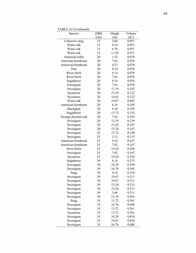
95
TABLE A2 (Continued).
Species DBH (cm
Height (m)
Volume 3) ) (m
Unknown s 66 .051 nag 15 3. 0Water oa 15 9.14 051 Water oa 15 6.10 051 Water oa 15 11.58 071 erican 20 1.52 6 can ho 20 7.62 6 can ho 20 4.57 6
Elm 20 9.14 076 River birc 20 9.14 076 River bi 20 7.62 6 Sugarber 20 9.14 6 Sweetgum 20 7.62 6 Sweetgum 20 12.19 2 Sycamore 20 15.24 122 Sycamore 20 14.63 122 Water oa 20 10.67 093 ican ho 20 6.10 105 Blackg 20 6.10 105 Sugarber 20 13.72 153
amp chestn 20 7.62 105 Sweetgum 20 12.19 139 Sweetgum 20 15.24 167 Sweetgum 20 15.24 167 Sweetgum 25 13.72 198 Sweetgum 25 2.13 133 ican hor 25 9.14 167
merican hor 25 7.62 167 River bi 25 15.24 9 Sweetgum 25 7.62 167 Sycamore 25 18.29 326
garber 30 9.14 275 Sweetgum 30 18.29 399
gum 30 16.76 365 Snag 30 9.14 8
Sweetgum 30 10.67 311 Sweetg 30 10.67 311 Sweetg 30 15.24 3 Sweetg 30 15.24 3 Sweetg 30 3.66 1 Sweetgum 30 12.19 6
Snag 35 13.72 1 Sweetg 35 16.76 8 Sweetg 35 13.72 1 Sycam 35 13.72 1 Sweetgum 35 18.29 0 Sweetgum 35 19.81 810
gum 35 16.76 688
k 0.k 0.k 0.
Am holly 0.07Ameri
merirnbeam r
0.0707A nbeam 0.
0.h 0.
rch 0.07ry 0.07
0.0710 0.
0.0.0.k
Amer rnbeam um
0.
ry 0.0.
Sw ut oak 0. 0. 0. 0. 0. 0.
Amer nbeam 0.A nbeam 0.
rch 0.26 0.
0.Su ry 0.
0.Sweet 0.
0.32 0.
um 0.um 0.51um 0.51um 0.31
0.41 0.56um 0.68um 0.56ore 0.56
0.81 0.
Sweet 0.

96
TABLE A2 (Continued). Species DBH
(cm) Height
(m) Volume
(m3)
Sycam 18.29 0.ore 35 810 Ash 40 21.34 1.1
Sw 0.892 Sw 40 0.892
amp 40 1.045 Sw 40 4 1.195 Sw 40 1.195 W 40 1.195 Sw 45 1 1.045 Sw 45 1.195 Wi 45 1.501
amp 50 1.841 Sw 55 1.943 W 55 1.943 Sw 55 8 2.483
Lobl 10 0.020 Lobl 10 0.020 Lobl 15 0.020 Lobl 20 0.074 Lobl 20 0.099 Lobl 30 0.671 Lobl 30 0.334 Lobl 35 4 0.736 Lobl 45 1.606
95 eetgum 40 16.76 eetgum 15.24
1 Sw chestnut oak 19.8eetgum 21.3eetgum 19.81
4 ater oak 21.3eetgum 19.8eetgum 21.34
4llow oak 21.3 Sw chestnut oak 21.34
eetgum 19.81 1 ater oak 19.8
eetgum 24.3olly pine 6.10
olly pine 2.44olly pine olly pine
2.13 6.10
olly pine olly pine
7.32 22.86
olly pine 10.67 olly pine 21.3olly pine 25.91
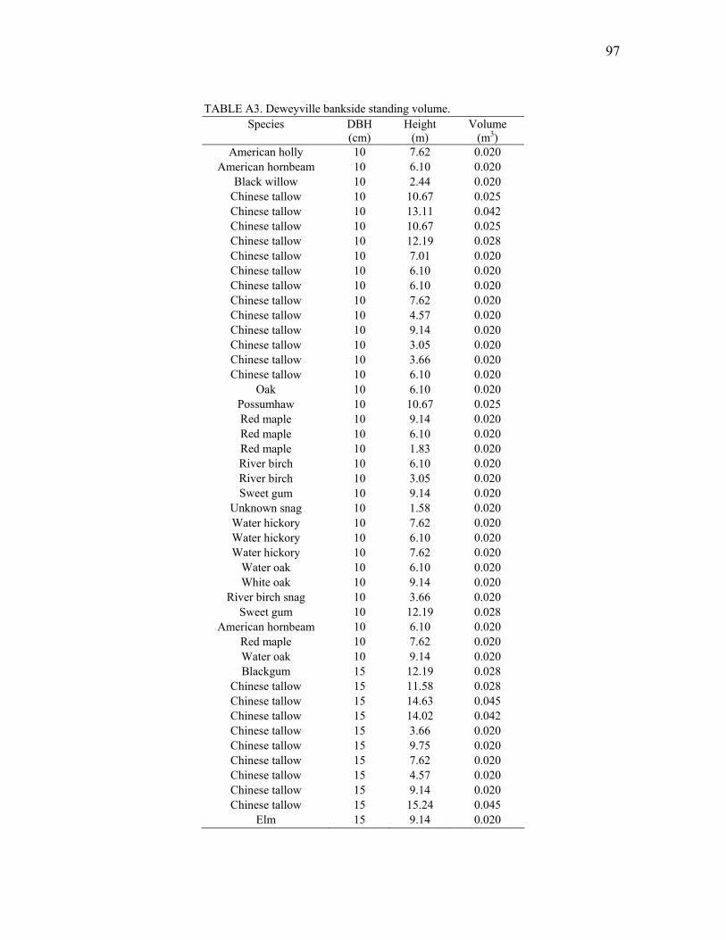
97
BLE A3. Deweyville bankside stan ng volume.
Species DBH (cm
ht )
lume 3)
TA di
) Heig
(mVo
(mAmerican holly 10 7.62 0.020
American horn 10 10 0.020 lack willow 10 2.44 .020 inese tallow 10 10.67 0.025 inese tallow 10 13.11 042
allow 10 10.67 5 allo 10 12.19 8 allo 10 7.01 0
ese tallo 10 6.10 0 inese tallow 10 6.10 020 inese tallow 10 7.62 0 inese tallow 10 4.57 0 inese tallow 10 9.14 020 inese tallow 10 3.05 020
allow 10 3.66 0.020 allow 10 6.10 020
ak 10 6.10 0 haw 10 10.67 5
maple 10 9.14 0 maple 10 6.10 0 maple 10 1.83 0 r birch 10 6.10 0 r birch 10 3.05 0 t gum 10 9.14 0
known snag 10 1.58 0 ater hickory 10 7.62 0 ater hickory 10 6.10 020
r hickory 10 7.62 020 ter oak 10 6.10 0.020
White oak 10 9.14 0.020 River birch snag 10 3.66 0.020
Sweet gum 10 12.19 0.028 American hornbeam 10 6.10 0.020
Red maple 10 7.62 0.020 Water oak 10 9.14 0.020 Blackgum 15 12.19 0.028
Chinese tallow 15 11.58 0.028 Chinese tallow 15 14.63 0.045 Chinese tallow 15 14.02 0.042 Chinese tallow 15 3.66 0.020 Chinese tallow 15 9.75 0.020 Chinese tallow 15 7.62 0.020 Chinese tallow 15 4.57 0.020 Chinese tallow 15 9.14 0.020 Chinese tallow 15 15.24 0.045
Elm 15 9.14 0.020
beam 6.B 0
Ch Ch 0.Chinese t 0.02Chinese t w 0.02Chinese t
inw w
0.0202Ch 0.
Ch 0.Ch 0.02
02Ch 0.Ch 0.Ch 0.Chinese t Chinese t
O 0.
0.020.02Possum
Red 0.02Red Red
0.020.02
RiveRive
0.020.02
Swee 0.020.02Un
W 0.02W 0.Wate
Wa 0.

98
TABLE A3 (Continued). Species DBH
(cm) Height
(m) Volume
(m3) Green ash 15 12.19 0.028 Red maple 15 10.67 0.025 Red maple 15 9.14 0.020 Red maple 15 6.71 0.020 Red maple 15 3.66 0.020 Red maple 15 4.57 0.020 Red maple 15 6.71 0.020 Red maple 15 12.19 0.028 Red maple 15 7.62 0.020 River birch 15 2.44 0.020 River birch 15 6.10 0.020 River birch 15 15.24 0.045
Tree sparkleberry 15 4.57 0.020 Tree sparkleberry 15 10.67 0.025 Tree sparkleberry 15 7.62 0.020
Water hickory 15 15.24 0.045 Water hickory 15 9.14 0.020 Water hickory 15 10.67 0.025 Water hickory 15 7.32 0.020 Water hickory 15 7.62 0.020
Water oak 15 6.10 0.020 Water oak 15 9.14 0.020
Winged elm 15 10.67 0.025 Sweetgum 15 9.75 0.020
Elm 15 7.62 0.051 Water hickory 15 9.14 0.051
Sweetgum 15 12.19 0.071 American hornbeam 15 7.62 0.051 American hornbeam 15 9.14 0.051 American hornbeam 15 9.14 0.051
ash 15 7.01 0.051 Chinese tallow 15 9.14 0.051 Chinese tallow 15 6.10 0.051 Chinese tallow 15 3.05 0.051 Chinese tallow 15 15.24 0.085 Chinese tallow 15 12.19 0.071 Chinese tallow 15 13.72 0.076
Chinese tallow snag 15 15.24 0.085 Elm 15 9.14 0.051 Elm 15 6.10 0.051 Elm 15 16.76 0.093
Green ash 15 13.72 0.076 Overcup oak 15 16.76 0.093 Possumhaw 15 6.10 0.051 Red maple 15 9.14 0.051 Red maple 15 13.72 0.076 Red maple 15 9.14 0.051

99
TABLE A3 (Continued). Species DBH
(cm) Height
(m) Volume
(m3) Red maple 15 9.14 0.051 Red maple 15 3.05 0.051 River birch 15 10.67 0.065 River birch 15 4.57 0.051 River birch 15 6.10 0.051 River birch 15 9.14 0.051 River birch 15 16.46 0.093 River birch 15 15.24 0.085 River birch 15 14.63 0.085 Sweet gum 15 9.14 0.051 Sweet gum 15 9.14 0.051 Sycamore 15 14.63 0.085 Sycamore 15 6.10 0.051 Sycamore 15 13.72 0.076 unknown 15 3.05 0.051
Unknown snag 15 3.05 0.051 Unknown snag 15 10.67 0.065 Water hickory 15 18.29 0.102 Water hickory 15 15.85 0.085 Water hickory 15 13.72 0.076
Water oak 15 7.62 0.051 Water oak 15 7.62 0.051 Water oak 15 13.72 0.076 Water oak 15 13.11 0.071
Winged elm 15 9.14 0.051 American hornbeam 15 9.14 0.051
Elm 15 12.19 0.071 Black gum 15 13.72 0.113
American hornbeam 15 7.62 0.076 Blackgum 20 12.19 0.102
Chinese tallow 20 9.14 0.076 Chinese tallow 20 16.76 0.136 Chinese tallow 20 4.88 0.076 Chinese tallow 20 13.72 0.113 Chinese tallow 20 3.66 0.076 Chinese tallow 20 10.67 0.093 Chinese tallow 20 10.67 0.093 Overcup oak 20 7.62 0.076 Red maple 20 13.72 0.113 River birch 20 18.29 0.147 Sweet gum 20 12.19 0.102 Sweetgum 20 10.67 0.093 Sycamore 20 13.72 0.113 Sycamore 20 7.01 0.076 unknown 20 1.68 0.076 Water oak 20 11.58 0.093
Winged elm 20 12.19 0.102
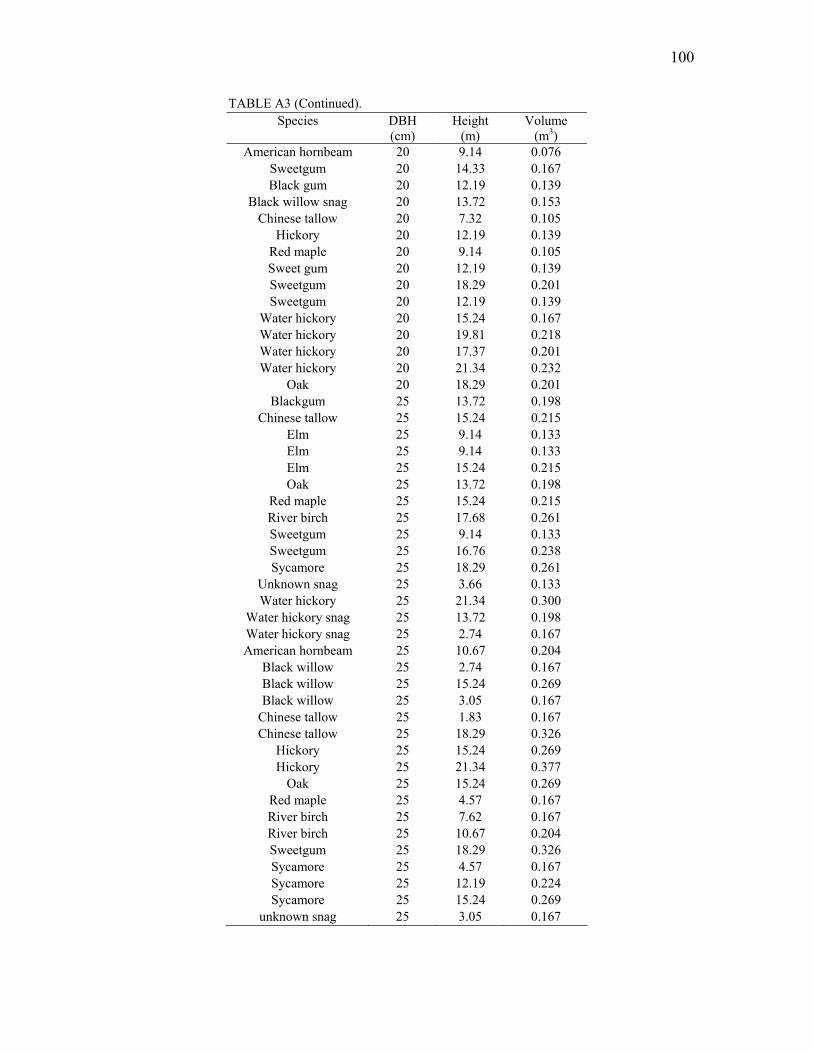
100
TABLE A3 (Continued). Species DBH
(cm) Height
(m) Volume
(m3) American hornbeam 20 9.14 0.076
Sweetgum 20 14.33 0.167 Black gum 20 12.19 0.139
Black willow snag 20 13.72 0.153 Chinese tallow 20 7.32 0.105
Hickory 20 12.19 0.139 Red maple 20 9.14 0.105 Sweet gum 20 12.19 0.139 Sweetgum 20 18.29 0.201 Sweetgum 20 12.19 0.139
Water hickory 20 15.24 0.167 Water hickory 20 19.81 0.218 Water hickory 20 17.37 0.201 Water hickory 20 21.34 0.232
Oak 20 18.29 0.201 Blackgum 25 13.72 0.198
Chinese tallow 25 15.24 0.215 Elm 25 9.14 0.133 Elm 25 9.14 0.133 Elm 25 15.24 0.215 Oak 25 13.72 0.198
Red maple 25 15.24 0.215 River birch 25 17.68 0.261 Sweetgum 25 9.14 0.133 Sweetgum 25 16.76 0.238 Sycamore 25 18.29 0.261
Unknown snag 25 3.66 0.133 Water hickory 25 21.34 0.300
Water hickory snag 25 13.72 0.198 Water hickory snag 25 2.74 0.167 American hornbeam 25 10.67 0.204
Black willow 25 2.74 0.167 Black willow 25 15.24 0.269 Black willow 25 3.05 0.167
Chinese tallow 25 1.83 0.167 Chinese tallow 25 18.29 0.326
Hickory 25 15.24 0.269 Hickory 25 21.34 0.377
Oak 25 15.24 0.269 Red maple 25 4.57 0.167 River birch 25 7.62 0.167 River birch 25 10.67 0.204 Sweetgum 25 18.29 0.326 Sycamore 25 4.57 0.167 Sycamore 25 12.19 0.224 Sycamore 25 15.24 0.269
unknown snag 25 3.05 0.167

101
TABLE A3 (Continued). Species DBH
(cm) Height
(m) Volume
(m3) Unknown snag 25 2.13 0.167 Water hickory 25 18.29 0.326 Water hickory 25 3.05 0.167 Water hickory 25 15.24 0.269
Water hickory snag 25 3.66 0.167 Water oak snag 25 12.19 0.275
American hornbeam 30 6.10 0.275 Black willow 30 19.81 0.430 Black willow 30 15.24 0.331
Chinese tallow 30 18.29 0.399 Elm 30 19.81 0.430
River birch 30 9.14 0.275 River birch 30 18.29 0.399 River birch 30 12.19 0.275
Water hickory 30 21.34 0.462 Water hickory 30 12.19 0.275 Water hickory 30 19.81 0.430 Water hickory 30 3.05 0.275
Sweetgum 30 18.29 0.399 Oak 30 12.19 0.275
Water hickory 30 18.29 0.399 Red maple 30 15.24 0.396
Snag 30 12.19 0.328 American hornbeam 30 12.19 0.328
Black willow 30 8.53 0.328 Elm 30 12.19 0.328 Oak 30 16.76 0.439
Overcup oak 30 21.34 0.552 River birch 30 6.10 0.328 Sweetgum 30 19.81 0.515
Water hickory 30 3.66 0.328 Water hickory 30 13.72 0.362 Water hickory 30 18.29 0.479
Water oak 30 9.14 0.328 Red maple 30 16.76 0.518
American hornbeam 30 10.67 0.388 Willow oak 30 12.19 0.388
Black willow 35 6.10 0.388 Black willow 35 6.10 0.388
Chinese tallow 35 16.15 0.467 Chinese tallow 35 18.29 0.564
River birch 35 12.19 0.388 River birch 35 18.29 0.564 Sweet gum 35 13.72 0.428 Sweet gum 35 19.81 0.609
Bald cypress 35 16.76 0.518 Water hickory 35 21.34 0.654

102
TABLE A3 (Continued). Species DBH
(cm) Height
(m) Volume
(m3) Water oak 35 3.93 0.388
Water oak snag 35 6.10 0.388 Black willow 35 9.14 0.388
Chinese tallow 35 3.05 0.544 Chinese tallow 35 7.92 0.544
Sycamore 35 18.29 0.657 Sycamore 35 16.76 0.603
Water hickory 35 24.38 0.858 Water hickory 35 18.29 0.657 Water hickory 35 18.29 0.657
Water oak 35 21.34 0.762 Water oak 35 21.34 0.762
Water oak snag 35 6.10 0.544 Sweet gum 35 7.38 0.629
Black willow 40 21.34 0.875 Black willow 40 19.81 0.818
Green ash 40 6.10 0.629 Overcup oak 40 13.11 0.629
Water hickory 40 22.86 1.065 Ash 40 12.19 0.716
Black willow 40 24.38 1.342 River birch 40 15.24 0.892
Water hickory 40 18.90 1.045 Water oak snag 40 18.29 1.045 Water hickory 40 22.86 1.342 Black willow 45 15.24 0.892 Sweet gum 45 18.29 1.045
Oak 45 25.91 1.863 Water hickory 45 24.38 1.682
Ash 45 24.38 1.682 Red oak 45 21.34 1.501
Sweetgum 45 19.81 1.501 Water hickory 45 17.98 1.314 Water oak snag 45 15.24 1.119
River birch 45 19.81 1.501 Water oak 50 22.25 1.501
Black willow 50 15.24 1.119 Water hickory 50 4.88 0.915
Oak 50 19.81 1.611 Ash 55 24.38 2.064
Black willow 55 13.72 1.376 Water hickory 55 25.91 2.282
Water oak 55 16.76 1.659 Water oak 55 24.38 2.483 Green ash 60 28.96 3.259 Sweet gum 65 22.86 3.078 Water oak 75 25.91 4.174

103
TABLE A4. Bon Wier Woody Debris Analysis Diameter
Log Number Length (ft) Butt Top Species Degree of
Decay Branch Presence 152 18.29 50.80 5.08 Water oak 1 Yes 153 3.66 30.48 10.16 unknown 3 Yes 154 6.10 20.32 5.08 unknown 3 Yes 155 3.05 30.48 5.08 unknown 3 No 156 6.10 38.10 5.08 unknown 3 No 157 14.63 30.48 17.78 Ash 2 Yes 158 7.62 17.78 5.08 unknown 3 Yes 159 4.57 15.24 5.08 American hornbeam 1 Yes 160 7.62 15.24 7.62 unknown 4 No 161 6.10 38.10 5.08 Water oak 2 Yes 162 2.13 25.40 5.08 Sweet gum 2 Yes 163 4.57 20.32 10.16 unknown 3 No 164 9.14 27.94 7.62 Elm 1 Yes 165 7.62 30.48 5.08 Sweet gum 1 Yes 166 5.49 38.10 15.24 Loblolly pine 3 No 167 3.66 10.16 30.48 unknown 3 No 168 9.14 20.32 76.20 Water oak 1 Yes 169 6.10 15.24 50.80 Maple 2 Yes 201 4.57 25.40 5.08 unknown 3 No 202 9.14 30.48 10.16 unknown 3 No 203 3.05 20.32 20.32 unknown 5 No 204 3.05 15.24 15.24 Loblolly pine 4 No 205 3.05 20.32 17.78 Loblolly pine 5 No 206 4.57 30.48 10.16 Loblolly pine 3 No 207 6.10 50.80 20.32 Loblolly pine 3 No 208 4.57 50.80 10.16 Loblolly pine 5 No 209 10.67 22.86 7.62 Sweet gum 1 No 210 12.19 35.56 7.62 Sycamore 1 Yes 211 4.57 20.32 5.08 American hornbeam 3 Yes 213 6.10 20.32 7.62 unknown 3 No 214 3.66 30.48 35.56 Loblolly pine 4 No 215 7.62 40.64 10.16 Sweet gum 1 No 216 6.10 40.64 10.16 unknown 5 No 217 3.66 30.48 35.56 Loblolly pine 4 No 218 3.05 30.48 35.56 Loblolly pine 4 No 219 3.66 25.40 25.40 Loblolly pine 4 No 220 3.66 25.40 35.56 Loblolly pine 3 No 221 3.05 22.86 5.08 unknown 4 No 222 4.57 20.32 5.08 unknown 4 No 223 7.62 20.32 5.08 unknown 4 No 224 4.57 10.16 5.08 unknown 4 No 225 9.14 50.80 10.16 unknown 3 No 226 5.49 30.48 7.62 American hornbeam 2 Yes 227 2.44 53.34 30.48 unknown 3 No

104
TABLE A4. (Continued).
Log Number Potential Source Origin Bank
Orientation Root Wad Position
Stage Contact
152 Cut Local 0 Yes Individual 1 153 Cut Local 0 Yes Individual 1 154 Cut Local 0 No Individual 1 155 unknown unknown 0 Unknown Individual 1 156 unknown unknown 0 Unknown Individual 1 157 Cut Local 0 Yes Individual 1 158 Cut Local 0 Yes Individual 1 159 Cut Local 0 Yes Individual 1 160 Cut unknown 0 Unknown Individual 1 161 Cut Local 0 Unknown Individual 1 162 Cut Local 0 Unknown Individual 1 163 Cut Local 0 Yes Individual 1 164 Cut Local 90 Yes Individual 1 165 Cut Local 90 Yes Individual 1 166 Windsnap Local 90 No Individual 1 167 unknown unknown 90 No Individual 1 168 Cut Local 90 Yes Jam 1 169 Cut Local 90 Yes Jam 1 201 Cut Local 90 Yes Individual 1 202 unknown Local 0 No Individual 1 203 unknown Local 0 Yes Individual 1 204 unknown Local 0 No Individual 1 205 unknown Local 90 No Individual 1 206 Windthrow Local 0 Yes Individual 1 207 Cut Local 0 Yes Individual 1 208 Cut unknown 0 Unknown Individual 1 209 unknown Local 0 Yes Individual 1 210 Cut Local 0 Yes Jam 1 211 Windthrow Local 180 Yes Jam 1 212 Cut Local 90 Yes Individual 1 213 Windthrow Local 0 No Individual 1 214 Cut Upstream 180 Unknown Individual 1 215 unknown Local 90 Yes Individual 1 216 Cut unknown 180 Yes Individual 1 217 unknown Upstream 180 Unknown Individual 1 218 unknown Upstream 180 Unknown Individual 1 219 unknown Upstream 180 Unknown Individual 1 220 unknown Local 90 Unknown Individual 1 221 unknown unknown 0 Unknown Individual 1 222 unknown unknown 0 Unknown Individual 1 223 unknown unknown 0 Unknown Individual 1 224 unknown unknown 0 Unknown Individual 1 225 Cut Local 90 Unknown Individual 1 226 Cut Local 90 Yes Jam 1 227 Windthrow Local 0 Yes Jam 1

105
TABLE A4. (Continued). Diameter
Log Number Length (ft) Butt Top Species Degree of
Decay Branch Presence 228 4.57 15.24 38.10 American hornbeam 1 Yes 229 1.83 20.32 15.24 Loblolly pine 4 No 230 4.57 10.16 38.10 Maple 2 Yes 400 7.62 30.48 20.32 unknown 3 No 401 4.57 30.48 20.32 Loblolly pine 4 No 402 9.14 20.32 5.08 unknown 3 Yes 403 4.57 25.40 5.08 unknown 4 Yes 404 6.10 30.48 10.16 River birch 4 No 405 11.58 33.02 10.16 unknown 3 No 406 1.83 20.32 20.32 Black willow 3 No 407 7.62 20.32 10.16 Black willow 3 No 408 4.57 20.32 7.62 Sycamore 2 Yes 409 6.10 25.40 7.62 unknown 4 No 410 6.10 30.48 10.16 Black willow 2 Yes 411 6.10 15.24 5.08 River birch 1 Yes 412 6.10 20.32 7.62 River birch 1 Yes 413 3.05 25.40 20.32 Loblolly pine 4 No 414 9.14 40.64 7.62 Black willow 2 Yes 415 10.67 30.48 5.08 Black willow 2 No 416 4.57 35.56 25.40 unknown 3 No 417 3.05 15.24 7.62 unknown 3 No 418 12.19 30.48 5.08 River birch 1 Yes 419 7.62 20.32 10.16 unknown 3 No 420 3.05 30.48 10.16 unknown 4 No 421 4.57 25.40 15.24 unknown 3 No 422 3.05 20.32 5.08 unknown 3 No 423 6.10 35.56 15.24 unknown 3 No 424 9.14 45.72 15.24 Bald cypress 3 No 425 3.05 20.32 5.08 unknown 4 No 426 4.57 30.48 20.32 unknown 3 No
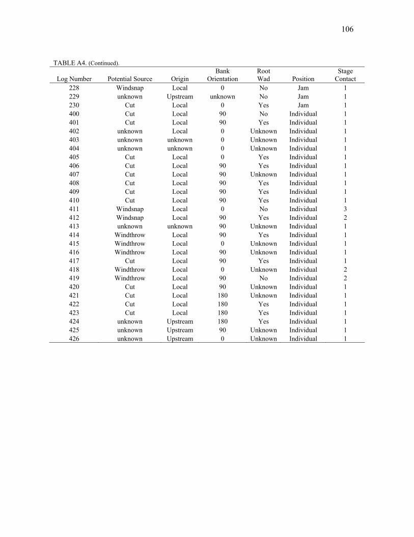
106
TABLE A4. (Continued).
Log Number Potential Source Origin Bank
Orientation Root Wad Position
Stage Contact
228 Windsnap Local 0 No Jam 1 229 unknown Upstream unknown No Jam 1 230 Cut Local 0 Yes Jam 1 400 Cut Local 90 No Individual 1 401 Cut Local 90 Yes Individual 1 402 unknown Local 0 Unknown Individual 1 403 unknown unknown 0 Unknown Individual 1 404 unknown unknown 0 Unknown Individual 1 405 Cut Local 0 Yes Individual 1 406 Cut Local 90 Yes Individual 1 407 Cut Local 90 Unknown Individual 1 408 Cut Local 90 Yes Individual 1 409 Cut Local 90 Yes Individual 1 410 Cut Local 90 Yes Individual 1 411 Windsnap Local 0 No Individual 3 412 Windsnap Local 90 Yes Individual 2 413 unknown unknown 90 Unknown Individual 1 414 Windthrow Local 90 Yes Individual 1 415 Windthrow Local 0 Unknown Individual 1 416 Windthrow Local 90 Unknown Individual 1 417 Cut Local 90 Yes Individual 1 418 Windthrow Local 0 Unknown Individual 2 419 Windthrow Local 90 No Individual 2 420 Cut Local 90 Unknown Individual 1 421 Cut Local 180 Unknown Individual 1 422 Cut Local 180 Yes Individual 1 423 Cut Local 180 Yes Individual 1 424 unknown Upstream 180 Yes Individual 1 425 unknown Upstream 90 Unknown Individual 1 426 unknown Upstream 0 Unknown Individual 1

107
TABLE A4. (Continued).
Diameter
Log Number Length (ft) Butt Top Species Degree of
Decay Branch Presence 427 7.62 30.48 5.08 unknown 3 No 428 6.10 40.64 10.16 unknown 3 No 429 4.57 30.48 15.24 unknown 3 No 430 7.62 30.48 15.24 unknown 3 No 431 10.67 40.64 5.08 River birch 1 Yes 432 6.10 35.56 5.08 unknown 1 Yes 433 3.66 45.72 25.40 Loblolly pine 3 No 434 10.67 35.56 5.08 Loblolly pine 2 Yes 435 6.10 30.48 15.24 oak 2 Yes 436 4.57 20.32 5.08 Sweet gum 2 No 437 6.10 38.10 5.08 unknown 3 Yes 438 3.05 30.48 15.24 unknown 4 No 439 6.10 25.40 10.16 unknown 3 No 440 4.57 30.48 20.32 Loblolly pine 3 No 441 7.62 30.48 5.08 River birch 1 Yes 442 4.57 50.80 50.80 Loblolly pine 5 No 443 7.62 30.48 5.08 unknown 3 No 444 7.62 38.10 5.08 unknown 3 Yes 445 6.10 25.40 15.24 Water oak 2 Yes 446 6.10 30.48 20.32 unknown 3 No

108
TABLE A4. (Continued).
Log Number Potential Source Origin Bank
Orientation Root Wad Position
Stage Contact
427 unknown unknown 0 Unknown Individual 1 428 unknown unknown 0 Yes Jam 1 429 unknown unknown 90 Unknown Jam 1 430 unknown unknown 180 Unknown Individual 1 431 Cut Local 0 Yes Jam 1 432 Cut Local 180 Yes Individual 1 433 Cut Local 90 Yes Individual 1 434 Cut Local 0 Yes Individual 1 435 Cut Local 180 Yes Individual 1 436 Cut Local 180 Yes Individual 1 437 unknown unknown 0 Unknown Individual 1 438 unknown unknown 180 Unknown Individual 1 439 unknown unknown 180 Yes Individual 1 440 unknown unknown 180 Unknown Individual 1 441 unknown Local 180 Unknown Individual 1 442 Windthrow Local 90 Unknown Individual 1 443 unknown unknown 180 Unknown Individual 1 444 unknown unknown 180 Unknown Individual 1 445 unknown unknown 180 No Individual 1 446 unknown unknown 180 No Individual 1

109
TABLE A5. Burkeville Woody Debris Analysis Diameter
Log Length Species Degree of Branch Number (ft) Butt Top Decay Presence
501 7.62 45.72 30.48 unknown 3 No 502 1.83 35.56 10.16 unknown 5 No 503 6.10 50.80 38.10 unknown 5 No 504 7.62 27.94 17.78 unknown 4 No 505 15.24 121.92 63.50 unknown 4 No 506 12.19 111.76 63.50 unknown 4 No 507 9.14 50.80 5.08 water oak 2 Yes 508 6.10 38.10 20.32 unknown 4 No 509 7.62 50.80 25.40 unknown 4 No 510 9.14 15.24 5.08 unknown 3 No 511 6.10 25.40 10.16 American hornbeam 3 No 512 6.10 106.68 35.56 unknown 3 No 513 4.57 25.40 15.24 unknown 3 No 514 4.57 30.48 10.16 unknown 4 No 515 4.57 15.24 15.24 unknown 3 No 516 3.05 20.32 27.94 unknown 3 No 517 12.19 40.64 10.16 Loblolly pine 2 Yes 518 4.57 50.80 35.56 unknown 3 No 519 8.53 22.86 7.62 unknown 2 No 520 12.19 63.50 5.08 unknown 3 Yes 521 6.10 20.32 15.24 Loblolly pine 3 No 522 4.57 25.40 15.24 Loblolly pine 4 No 523 6.10 30.48 20.32 unknown 3 No 524 4.57 35.56 20.32 Loblolly pine 3 No 525 6.10 30.48 5.08 Loblolly pine 1 Yes 526 4.57 40.64 25.40 Loblolly pine 1 Yes 527 9.14 50.80 25.40 Loblolly pine 1 Yes 528 7.62 17.78 5.08 unknown 3 Yes 529 6.10 25.40 10.16 unknown 3 No 530 9.14 45.72 10.16 unknown 3 No 531 6.10 50.80 20.32 unknown 3 No 532 3.05 20.32 20.32 unknown 4 No 533 9.14 38.10 15.24 unknown 3 No 534 6.71 50.80 25.40 unknown 3 No 535 3.05 20.32 15.24 unknown 3 No 536 6.10 20.32 12.70 unknown 3 No

110
TABLE A5. (Continued).
Log Potential Origin Bank Root Position Stage Number Source Orientation Wad Contact
501 Cut Local 0 Yes Fallen tree 1 502 Cut Local 180 Yes Fallen tree 1 503 Cut Local 90 Yes Fallen tree 1 504 Cut Local 0 No Fallen tree 1 505 Cut Local 0 Yes Fallen tree 1 506 Unknown Upstream 0 Yes Individual 1 507 Cut Local 0 Yes Fallen tree 1 508 Cut Local 0 Yes Fallen tree 1 509 Cut Local 90 Yes Fallen tree 1 510 Unknown Upstream 0 Unknown Individual 1 511 Unknown Upstream 0 Unknown Individual 1 512 Unknown Upstream 90 Yes Individual 1 513 Unknown Upstream 90 No Jam 1 514 Unknown Upstream 180 No Individual 1 515 Unknown Upstream 0 Yes Jam 1 516 Unknown Upstream 90 No Jam 1 517 Unknown Upstream 90 Yes Individual 1 518 Unknown Upstream 0 No Jam 1 519 Unknown Upstream 0 No Jam 1 520 Unknown Upstream 90 Unknown Jam 1 521 Unknown Upstream 0 No Jam 1 522 Unknown Upstream 0 No Jam 1 523 Unknown Upstream 0 No Jam 1 524 Cut Local 90 Yes Fallen tree 3 525 Cut Local 0 Yes Fallen tree 2 526 Cut Local 90 Yes Fallen tree 4 527 Cut Local 180 Yes Fallen tree 3 528 Unknown Upstream 0 Unknown individual 1 529 Unknown Upstream 0 No individual 1 530 Unknown Upstream 0 No individual 1 531 Unknown Upstream 0 Yes individual 1 532 Unknown Upstream 180 Unknown individual 1 533 Unknown Upstream 0 Yes Jam 1 534 Unknown Upstream 90 No Jam 1 535 Unknown Upstream 0 No Jam 1 536 Unknown Upstream 0 No Jam 1

111
TABLE A5. (Continued). Diameter
Log Length Species Degree of Branch Number (ft) Butt Top Decay Presence
537 3.66 20.32 10.16 unknown 3 No 538 4.27 63.50 40.64 Loblolly pine 2 No 539 15.24 114.30 25.40 Sweet gum 2 Yes 540 9.14 38.10 5.08 water oak 1 Yes 541 9.14 25.40 7.62 Loblolly pine 1 Yes 542 5.49 50.80 15.24 unknown 3 Yes 543 7.62 40.64 7.62 unknown 3 No 544 5.49 25.40 5.08 unknown 3 Yes 545 5.49 20.32 5.08 unknown 3 Yes 546 4.27 25.40 20.32 unknown 3 No 547 10.67 45.72 10.16 unknown 2 Yes 548 9.14 45.72 10.16 Sweet gum 2 Yes 549 6.10 20.32 5.08 Loblolly pine 2 Yes 550 10.67 40.64 5.08 Loblolly pine 2 Yes 551 9.14 40.64 5.08 Sweet gum 1 Yes 552 2.44 20.32 10.16 unknown 3 No 553 4.88 20.32 7.62 unknown 3 No 554 6.71 25.40 15.24 unknown 4 No 555 7.62 40.64 7.62 unknown 3 No 556 7.32 30.48 5.08 hickory 3 Yes 557 12.80 149.86 76.20 unknown 3 No 558 7.62 35.56 15.24 Black tupelo 1 Yes 559 2.44 55.88 30.48 unknown 2 No 560 5.18 30.48 15.24 unknown 3 No 561 7.62 30.48 30.48 unknown 3 No 562 9.75 50.80 10.16 unknown 4 No 563 6.10 25.40 10.16 unknown 4 No 564 4.57 50.80 25.40 unknown 3 No 565 4.57 20.32 5.08 unknown 2 Yes 566 7.62 33.02 5.08 unknown 3 Yes 567 10.67 50.80 10.16 water oak 2 Yes 568 7.62 40.64 10.16 unknown 3 Yes 569 9.14 45.72 20.32 unknown 2 Yes 570 6.71 20.32 10.16 Loblolly pine 4 No 571 8.23 53.34 15.24 Sweet gum 3 Yes 572 6.10 35.56 15.24 unknown 3 No 573 2.13 30.48 22.86 unknown 3 Yes

112
TABLE A5. (Continued).
Log Potential Origin Bank Root Position Stage Number Source Orientation Wad Contact
537 Unknown Upstream 90 No Jam 1 538 Cut Local 180 Yes Jam 1 539 Cut Local 0 Yes Fallen tree 2 540 Cut Local 0 Yes Fallen tree 2 541 Cut Local 0 Yes Fallen tree 2 542 Cut Local 180 Yes Fallen tree 2 543 Cut Local 0 Yes Jam 2 544 Cut Local 180 Yes Jam 2 545 Cut Local 180 Yes Jam 2 546 Unknown Local 90 No Jam 1 547 Cut Local 0 Yes Fallen tree 2 548 Cut Local 0 Yes Fallen tree 2 549 Cut Local 90 Yes Fallen tree 2 550 Cut Local 180 Yes Fallen tree 2 551 Cut Local 90 Yes Fallen tree 2 552 Unknown Unknown 90 No Jam 1 553 Unknown Unknown 0 No Jam 1 554 Unknown Unknown 0 No Jam 1 555 Unknown Unknown 0 No Jam 1 556 Unknown Unknown 0 Yes individual 1 557 Cut Local 0 No Fallen tree 1 558 Cut Local 0 No Fallen tree 2 559 Cut Local 90 Yes Fallen tree 1 560 Unknown Unknown 0 Yes Jam 1 561 Unknown Upstream 0 No individual 1 562 Unknown Upstream 0 No individual 1 563 Unknown Upstream 90 Yes individual 1 564 Unknown Upstream 0 Unknown individual 1 565 Cut Local 0 Yes Fallen tree 1 566 Unknown Upstream 0 Unknown individual 1 567 Cut Local 0 Yes Fallen tree 1 568 Cut Local 0 Yes Fallen tree 1 569 Cut Local 0 Yes Fallen tree 1 570 Cut Local 90 Yes Fallen tree 1 571 Cut Local 90 Yes Fallen tree 1 572 Unknown Upstream 0 Yes Jam 1 573 Unknown Upstream 0 Yes Jam 1

113
TABLE A5. (Continued). Diameter
Log Length Species Degree of Branch Number (ft) Butt Top Decay Presence
574 6.10 22.86 20.32 water oak 2 Yes 575 12.19 25.40 10.16 Bald cypress 4 Yes 576 4.88 20.32 10.16 unknown 4 No 577 6.10 25.40 5.08 unknown 4 No 578 6.10 63.50 25.40 unknown 4 No 579 4.57 45.72 45.72 water oak 3 No 580 6.10 50.80 15.24 Sweet gum 3 Yes 581 15.24 50.80 5.08 Loblolly pine 2 Yes 582 19.81 101.60 5.08 Ash 2 Yes 583 6.10 25.40 5.08 unknown 3 Yes 584 2.44 15.24 5.08 unknown 3 No 585 9.14 50.80 5.08 unknown 3 Yes 586 6.10 15.24 10.16 unknown 3 Yes 587 9.14 45.72 10.16 unknown 3 Yes 588 6.10 25.40 10.16 unknown 4 Yes 589 6.10 15.24 7.62 unknown 3 Yes 590 12.19 45.72 20.32 unknown 3 Yes 591 9.14 30.48 12.70 Sweet gum 2 Yes 592 12.19 114.30 12.70 unknown 2 Yes 593 2.13 30.48 10.16 unknown 5 No

114
TABLE A5. (Continued).
Log Potential Origin Bank Root Position Stage Number Source Orientation Wad Contact
574 Unknown Upstream 0 Yes Jam 1 575 Unknown Upstream 0 Yes individual 1 576 Unknown Upstream 90 Unknown Jam 1 577 Unknown Upstream 90 Unknown Jam 1 578 Unknown Upstream 90 Unknown Jam 1 579 Cut Local 90 Yes Jam 1 580 Cut Local 0 Yes Fallen tree 1 581 Cut Local 0 Yes Fallen tree 1 582 Unknown Upstream 0 Unknown individual 1 583 Unknown Upstream 0 Unknown individual 1 584 Unknown Upstream 0 Unknown individual 1 585 Unknown Upstream 90 Unknown individual 1 586 Unknown Upstream 90 Yes individual 1 587 Unknown Upstream 0 Yes individual 1 588 Unknown Upstream 90 Yes individual 1 589 Unknown Upstream 0 Unknown individual 1 590 Cut Local 0 Yes Jam 1 591 Cut Local 90 Yes Jam 1 592 Cut Local 90 Yes Jam 1 593 Cut Local 0 Unknown individual 1

115
TABLE A6. Deweyville Woody Debris Analysis Diameter
Log Length Species Degree of Branch Number (ft) Butt Top Decay Presence
101 9.14 30.48 34.29 Unknown 3 No 102 4.57 35.81 28.70 Unknown 3 No 103 3.05 30.48 22.86 Unknown 3 No 104 3.35 25.40 15.24 Unknown 3 No 105 9.14 20.32 7.62 Chinese tallow 1 Yes 106 12.19 25.40 12.70 River birch 1 Yes 107 2.44 12.70 12.70 Unknown 4 No 108 4.57 35.56 30.48 Unknown 5 No 109 4.57 35.56 30.48 Unknown 3 No 110 6.10 38.10 20.32 Elm 3 No 111 7.62 15.24 5.08 Unknown 1 Yes 112 6.10 15.24 5.08 Unknown 1 Yes 113 12.19 17.78 5.08 Black willow 3 Yes 114 7.62 22.86 10.16 Unknown 2 No 115 15.24 69.09 45.72 Oak 4 No 116 9.14 22.86 7.62 Sweet gum 3 Yes 117 6.10 43.18 38.10 Unknown 4 No 118 2.13 25.40 20.32 Unknown 4 No 119 6.10 15.24 7.62 River birch 1 Yes 120 3.66 36.58 25.40 Unknown 3 No 121 6.10 17.78 10.16 Unknown 4 No 122 7.62 26.92 12.70 Chinese tallow 3 Yes 123 2.44 25.40 25.40 Unknown 4 No 124 3.35 22.86 10.16 Unknown 4 No 125 4.57 20.32 5.08 Unknown 3 Yes 126 6.10 25.40 25.40 Unknown 2 Yes 127 6.10 35.56 25.40 Unknown 3 No 128 15.24 43.18 25.40 Black willow 1 Yes 129 4.57 12.70 10.16 Unknown 3 Yes 130 6.10 33.78 5.08 Elm 2 Yes 131 6.10 38.10 25.40 Chinese tallow 3 No 132 12.19 45.72 17.78 River birch 2 Yes 133 6.10 30.48 12.70 River birch 2 Yes 134 16.76 38.10 15.24 River birch 2 Yes 135 12.19 22.86 5.08 Unknown 2 Yes 136 12.19 30.48 12.70 Unknown 3 Yes

116
TABLE A6. (Continued).
Log Potential Origin Bank Root Position Stage Number Source Orientation Wad Contact
101 Unknown Unknown 90 No Ind piece 2 102 Unknown Unknown 90 No Ind piece 2 103 Unknown Unknown 90 No Ind piece 1 104 Unknown Unknown 180 Yes Ind piece 3 105 Cut Local 90 Yes Ind piece 2 106 Cut Local 90 Yes Ind piece 2 107 Unknown Unknown Unknown No Ind piece 4 108 Unknown Unknown Unknown No Jam 4 109 Unknown Unknown Unknown No Jam 4 110 Unknown Unknown Unknown No Jam 4 111 Windthrow Local 0 Yes Fallen tree 1 112 Windthrow Local 90 Yes Fallen tree 1 113 Unknown Unknown 180 Unknown Fallen tree 1 114 Unknown Unknown 90 Yes Fallen tree 1 115 Unknown Unknown 90 Yes Fallen tree 1 116 Unknown Unknown 90 Yes Fallen tree 1 117 Unknown Unknown 0 No Ind piece 1 118 Unknown Unknown 90 No Ind piece 1 119 Unknown Unknown 90 Unknown Fallen tree 1 120 Unknown Unknown 180 Yes Fallen tree 1 121 Unknown Unknown 90 No Ind piece 1 122 Unknown Unknown 0 Yes Fallen tree 1 123 Unknown Unknown 180 No Ind piece 2 124 Unknown Unknown 180 No Ind piece 3 125 Unknown Unknown 90 No Ind piece 2 126 Unknown Unknown 90 Unknown Fallen tree 1 127 Unknown Unknown 90 Yes Ind piece 1 128 Windsnap Local 90 Yes Fallen tree 2 129 Unknown Unknown 180 No Ind piece 2 130 Unknown Unknown 90 Yes Fallen tree 1 131 Unknown Local 90 Yes Fallen tree 1 132 Unknown Local 90 Yes Fallen tree 3 133 Unknown Local 180 Yes Fallen tree 3 134 Unknown Local 0 Yes Fallen tree 1 135 Unknown Local 180 Yes Fallen tree 3 136 Unknown Local 0 Unknown Fallen tree 1

117
TABLE A6. (Continued). Diameter
Log Length Species Degree of Branch Number (ft) Butt Top Decay Presence
137 3.66 20.32 10.16 Unknown 4 No 138 9.14 30.48 27.94 Unknown 2 Yes 139 12.19 52.32 20.32 Unknown 2 Yes 140 1.98 31.24 30.48 Unknown 3 No 141 7.62 38.10 26.42 Unknown 3 No 142 6.10 35.56 7.62 Unknown 2 No 143 4.57 30.48 15.24 Unknown 2 Yes 144 9.14 10.16 20.32 Unknown 2 No 145 7.62 17.78 10.16 Unknown 2 Yes 146 10.67 25.40 5.08 Unknown 2 Yes 147 4.57 10.16 20.32 Chinese tallow 2 Yes 148 3.05 10.16 20.32 Unknown 2 Yes 149 6.10 27.94 5.08 Unknown 3 Yes 151 3.05 12.70 12.70 Unknown 4 No 232 2.44 20.32 15.24 Unknown 4 No 233 13.72 30.48 10.16 Unknown 3 No 234 15.24 30.48 10.16 Chinese tallow 2 No 235 6.10 25.40 15.24 Unknown 4 No 236 6.10 20.32 15.24 Unknown 3 No 237 4.57 15.24 10.16 Unknown 3 No 238 13.72 17.78 5.08 Unknown 3 Yes 239 4.57 15.24 5.08 Unknown 3 No 240 4.57 15.24 10.16 Unknown 3 No 241 3.66 33.02 33.02 Unknown 4 No 242 3.66 25.40 10.16 Unknown 4 No 243 4.57 25.40 20.32 Unknown 3 No 244 6.10 15.24 10.16 Unknown 3 No 245 6.10 33.02 20.32 Unknown 4 No 246 12.19 40.64 30.48 Black willow 3 Yes 247 6.10 15.24 15.24 Unknown 3 No 248 6.10 30.48 5.08 Black willow 2 Yes 249 4.57 25.40 12.70 Unknown 4 No 250 7.62 25.40 5.08 American hornbeam 1 Yes 251 4.57 35.56 15.24 Unknown 3 No 252 7.62 20.32 15.24 Unknown 3 Yes 253 2.44 30.48 20.32 Unknown 3 No 254 6.10 20.32 12.70 Unknown 2 Yes 255 15.24 30.48 5.08 Black willow 2 Yes 256 4.57 25.40 15.24 Sweet gum 2 No 257 7.62 20.32 10.16 Unknown 3 Yes 258 7.62 20.32 5.08 Unknown 3 Yes 259 13.72 40.64 5.08 Unknown 1 Yes 260 6.10 20.32 10.16 Unknown 3 No 261 6.10 20.32 7.62 Unknown 3 No

118
TABLE A6. (Continued).
Log Potential Origin Bank Root Position Stage Number Source Orientation Wad Contact
137 Unknown Local 90 No Ind piece 4 138 Unknown Local 180 Yes Fallen tree 1 139 Unknown Local 180 Yes Fallen tree 1 140 Unknown Local 90 No Ind piece 2 141 Unknown Unknown 180 No Ind piece 1 142 Unknown Unknown 0 No Ind piece 1 143 Unknown Unknown 0 Yes Fallen tree 1 144 Unknown Unknown 0 Unknown Fallen tree 1 145 Unknown Unknown 0 Yes Fallen tree 1 146 Unknown Local 0 Yes Fallen tree 2 147 Unknown Local 0 Yes Fallen tree 2 148 Unknown Unknown 0 Unknown Ind piece 1 149 Windthrow Unknown 90 Yes Ind piece 1 151 Unknown Unknown 90 No Ind piece 1 232 Cut Local 90 Yes Jam 1 233 Cut Local 0 Yes Jam 1 234 Cut Local 0 Yes Jam 1 235 Unknown Local 90 Yes Ind piece 1 236 Windsnap Local 90 No Ind piece 2 237 Windsnap Local 90 No Ind piece 2 238 Windsnap Local 90 No Fallen tree 3 239 Unknown Unknown 90 No Jam 2 240 Unknown Unknown 90 No Jam 2 241 Unknown unknown 90 Yes Jam 2 242 Unknown Unknown 90 No Jam 2 243 Unknown Unknown 90 No Jam 2 244 Unknown Unknown 90 Yes Jam 2 245 Unknown Unknown 0 Yes Jam 2 246 Windsnap Local 90 No Fallen tree 3 247 Cut Local 90 Yes Fallen tree 3 248 Cut Local 90 Yes Fallen tree 3 249 Unknown Unknown 90 No Ind piece 1 250 Cut Local 90 Yes Fallen tree 2 251 Cut Local 90 Yes Fallen tree 1 252 Unknown Unknown 180 Unknown Ind piece 1 253 Unknown Unknown 180 No Ind piece 1 254 Cut Local 90 Yes Fallen tree 1 255 Cut Local 0 Yes Fallen tree 1 256 Unknown Unknown 0 Yes Jam 1 257 Unknown Local 0 Yes Fallen tree 1 258 Unknown Unknown 0 Unknown Jam 1 259 Cut Local 0 Yes Jam 1 260 Unknown Unknown 180 Yes Ind piece 1 261 Unknown Unknown 180 No Jam 1

119
TABLE A6. (Continued). Diameter
Log Length Species Degree of Branch Number (ft) Butt Top Decay Presence
262 7.62 30.48 10.16 Unknown 4 No 263 7.62 33.02 7.62 Unknown 2 No 264 15.24 40.64 5.08 Sycamore 1 Yes 265 4.57 50.80 25.40 Unknown 4 No 266 9.14 33.02 30.48 Unknown 3 No 267 12.19 20.32 5.08 Unknown 2 Yes 268 4.57 50.80 45.72 Unknown 4 No 269 4.57 25.40 20.32 Unknown 4 No 270 7.62 30.48 20.32 Unknown 4 No 271 9.14 50.80 5.08 Unknown 3 Yes 272 4.57 45.72 15.24 Unknown 4 No 273 9.14 30.48 30.48 Unknown 3 No 274 12.19 35.56 20.32 Bald cypress 3 No 275 12.19 55.88 20.32 Unknown 3 No 276 7.62 25.40 5.08 Ash 3 Yes 277 7.62 33.02 25.40 Pine 4 No 278 4.57 15.24 15.24 Unknown 4 No 279 6.10 27.94 22.86 Unknown 4 No 280 7.62 35.56 20.32 Pine 3 No 281 10.67 40.64 20.32 Pine 3 No 282 9.14 40.64 5.08 Unknown 1 Yes 283 9.14 40.64 20.32 Unknown 4 No 284 9.75 17.78 10.16 Unknown 4 No 285 9.14 25.40 5.08 American elm 1 Yes 286 9.14 25.40 5.08 Slippery elm 1 Yes 287 1.52 30.48 25.40 Unknown 4 No 288 10.67 30.48 7.62 Water oak 1 Yes 289 15.24 30.48 7.62 Sweet gum 1 Yes 290 21.34 30.48 5.08 Unknown 1 Yes 291 10.67 66.04 25.40 Unknown 4 No 292 7.62 35.56 22.86 Unknown 3 No 293 10.67 48.26 25.40 Unknown 4 No 294 6.10 38.10 27.94 Unknown 2 No 295 6.10 15.24 5.08 Oak 1 Yes 296 5.49 38.10 15.24 Unknown 3 No 297 2.13 27.94 27.94 Unknown 4 No 298 3.05 22.86 22.86 Unknown 4 No 299 6.10 20.32 5.08 Unknown 3 Yes 300 7.62 20.32 5.08 River birch 1 Yes

120
TABLE A6. (Continued).
Log Potential Origin Bank Root Position Stage Number Source Orientation Wad Contact
262 Unknown Unknown 180 No Jam 1 263 Unknown Unknown 180 Yes Jam 1 264 Windthrow Local 0 Yes Fallen tree 4 265 Unknown Unknown 90 No Jam 1 266 Windsnap Local 0 No Fallen tree 1 267 Windsnap Local 90 Yes Fallen tree 1 268 Unknown Unknown 0 Unknown Jam 1 269 Unknown Unknown 0 Yes Jam 1 270 Unknown Unknown 0 Unknown Jam 1 271 Cut Local 90 Unknown Jam 1 272 Unknown Unknown 0 Yes Jam 1 273 Unknown Unknown 90 Unknown Jam 1 274 Unknown Unknown 0 Unknown Jam 1 275 Unknown Local 180 Yes Jam 1 276 Windthrow Local 90 Yes Fallen tree 1 277 Unknown Unknown 90 No Jam 1 278 Unknown Upstream 180 No Jam 1 279 Unknown Upstream 180 No Jam 1 280 Unknown Unknown 0 No Jam 1 281 Unknown Unknown 180 No Jam 1 282 Windthrow Local 0 Yes Fallen tree 2 283 Unknown Unknown 0 No Jam 1 284 Unknown Unknown 180 No Jam 1 285 Windthrow Local 0 Yes Fallen tree 4 286 Windthrow Local 0 Yes Fallen tree 2 287 Unknown Unknown 0 Yes Jam 2 288 Windthrow Local 180 Yes Fallen tree 1 289 Windthrow Local 180 Yes Fallen tree 1 290 Windthrow Local 0 Yes Fallen tree 1 291 Cut Local 0 No Jam 1 292 Windthrow Unknown 180 Yes Jam 1 293 Windthrow Local 90 Yes Fallen tree 1 294 Windthrow Local 90 Yes Fallen tree 1 295 Cut Local 180 Yes Fallen tree 1 296 Unknown Unknown 90 Yes Ind piece 1 297 Unknown Local 90 Unknown Fallen tree 1 298 Unknown Local 90 Unknown Fallen tree 1 299 Unknown Unknown 90 Unknown Ind piece 1 300 Unknown Local 90 Yes Fallen tree 2
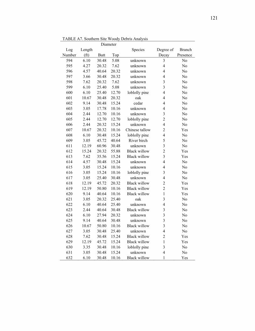
121
TABLE A7. Southern Site Woody Debris Analysis Diameter
Log Length Species Degree of Branch Number (ft) Butt Top Decay Presence
594 6.10 30.48 5.08 unknown 3 No 595 4.27 20.32 7.62 unknown 4 No 596 4.57 40.64 20.32 unknown 4 No 597 3.66 30.48 20.32 unknown 4 No 598 7.62 20.32 7.62 unknown 3 No 599 6.10 25.40 5.08 unknown 3 No 600 6.10 25.40 12.70 loblolly pine 4 No 601 10.67 30.48 20.32 oak 4 No 602 9.14 30.48 15.24 cedar 4 No 603 3.05 17.78 10.16 unknown 4 No 604 2.44 12.70 10.16 unknown 3 No 605 2.44 12.70 12.70 loblolly pine 2 No 606 2.44 20.32 15.24 unknown 4 No 607 10.67 20.32 10.16 Chinese tallow 2 Yes 608 6.10 30.48 15.24 loblolly pine 4 No 609 3.05 45.72 40.64 River birch 5 No 611 12.19 60.96 30.48 unknown 3 No 612 15.24 20.32 55.88 Black willow 2 Yes 613 7.62 35.56 15.24 Black willow 3 Yes 614 4.57 30.48 15.24 unknown 4 No 615 3.05 15.24 10.16 unknown 4 No 616 3.05 15.24 10.16 loblolly pine 3 No 617 3.05 25.40 30.48 unknown 4 No 618 12.19 45.72 20.32 Black willow 2 Yes 619 12.19 50.80 10.16 Black willow 2 Yes 620 9.14 40.64 10.16 Black willow 1 Yes 621 3.05 20.32 25.40 oak 3 No 622 6.10 40.64 25.40 unknown 4 No 623 2.44 40.64 30.48 Black willow 3 No 624 6.10 27.94 20.32 unknown 3 No 625 9.14 40.64 30.48 unknown 3 No 626 10.67 50.80 10.16 Black willow 3 No 627 3.05 30.48 25.40 unknown 4 No 628 7.62 30.48 15.24 Black willow 2 Yes 629 12.19 45.72 15.24 Black willow 1 Yes 630 3.35 30.48 10.16 loblolly pine 3 No 631 3.05 30.48 15.24 unknown 4 No 632 6.10 30.48 10.16 Black willow 1 Yes
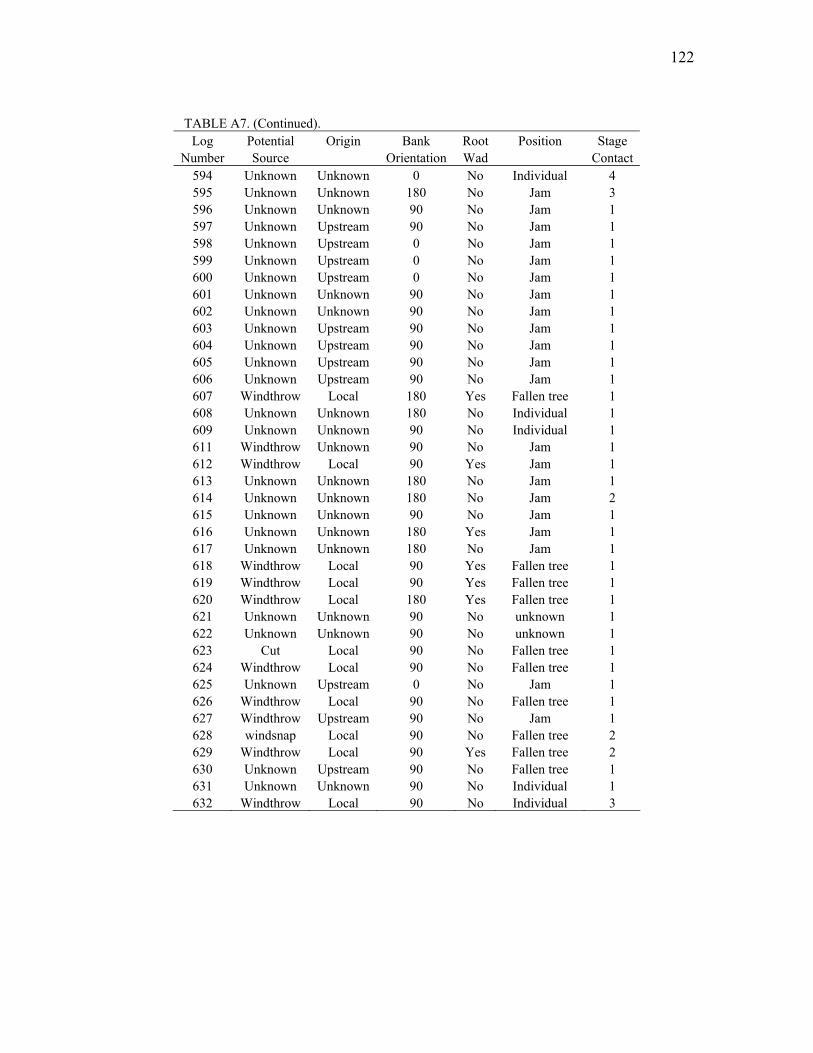
122
TABLE A7. (Continued).
Log Potential Origin Bank Root Position Stage Number Source Orientation Wad Contact
594 Unknown Unknown 0 No Individual 4 595 Unknown Unknown 180 No Jam 3 596 Unknown Unknown 90 No Jam 1 597 Unknown Upstream 90 No Jam 1 598 Unknown Upstream 0 No Jam 1 599 Unknown Upstream 0 No Jam 1 600 Unknown Upstream 0 No Jam 1 601 Unknown Unknown 90 No Jam 1 602 Unknown Unknown 90 No Jam 1 603 Unknown Upstream 90 No Jam 1 604 Unknown Upstream 90 No Jam 1 605 Unknown Upstream 90 No Jam 1 606 Unknown Upstream 90 No Jam 1 607 Windthrow Local 180 Yes Fallen tree 1 608 Unknown Unknown 180 No Individual 1 609 Unknown Unknown 90 No Individual 1 611 Windthrow Unknown 90 No Jam 1 612 Windthrow Local 90 Yes Jam 1 613 Unknown Unknown 180 No Jam 1 614 Unknown Unknown 180 No Jam 2 615 Unknown Unknown 90 No Jam 1 616 Unknown Unknown 180 Yes Jam 1 617 Unknown Unknown 180 No Jam 1 618 Windthrow Local 90 Yes Fallen tree 1 619 Windthrow Local 90 Yes Fallen tree 1 620 Windthrow Local 180 Yes Fallen tree 1 621 Unknown Unknown 90 No unknown 1 622 Unknown Unknown 90 No unknown 1 623 Cut Local 90 No Fallen tree 1 624 Windthrow Local 90 No Fallen tree 1 625 Unknown Upstream 0 No Jam 1 626 Windthrow Local 90 No Fallen tree 1 627 Windthrow Upstream 90 No Jam 1 628 windsnap Local 90 No Fallen tree 2 629 Windthrow Local 90 Yes Fallen tree 2 630 Unknown Upstream 90 No Fallen tree 1 631 Unknown Unknown 90 No Individual 1 632 Windthrow Local 90 No Individual 3
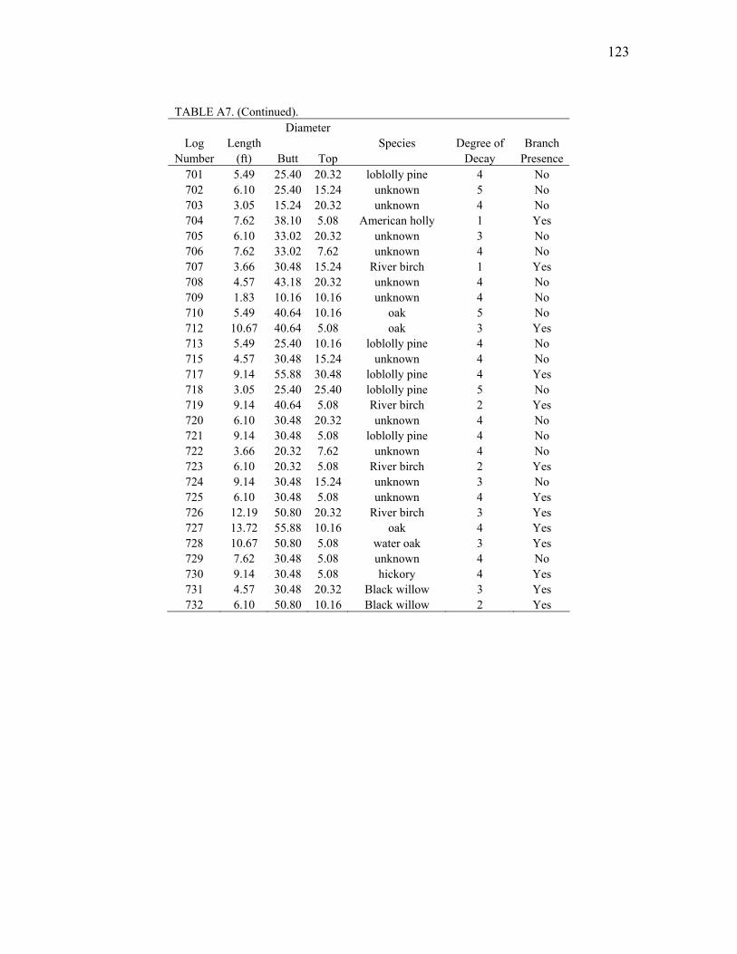
123
TABLE A7. (Continued). Diameter
Log Length Species Degree of Branch Number (ft) Butt Top Decay Presence
701 5.49 25.40 20.32 loblolly pine 4 No 702 6.10 25.40 15.24 unknown 5 No 703 3.05 15.24 20.32 unknown 4 No 704 7.62 38.10 5.08 American holly 1 Yes 705 6.10 33.02 20.32 unknown 3 No 706 7.62 33.02 7.62 unknown 4 No 707 3.66 30.48 15.24 River birch 1 Yes 708 4.57 43.18 20.32 unknown 4 No 709 1.83 10.16 10.16 unknown 4 No 710 5.49 40.64 10.16 oak 5 No 712 10.67 40.64 5.08 oak 3 Yes 713 5.49 25.40 10.16 loblolly pine 4 No 715 4.57 30.48 15.24 unknown 4 No 717 9.14 55.88 30.48 loblolly pine 4 Yes 718 3.05 25.40 25.40 loblolly pine 5 No 719 9.14 40.64 5.08 River birch 2 Yes 720 6.10 30.48 20.32 unknown 4 No 721 9.14 30.48 5.08 loblolly pine 4 No 722 3.66 20.32 7.62 unknown 4 No 723 6.10 20.32 5.08 River birch 2 Yes 724 9.14 30.48 15.24 unknown 3 No 725 6.10 30.48 5.08 unknown 4 Yes 726 12.19 50.80 20.32 River birch 3 Yes 727 13.72 55.88 10.16 oak 4 Yes 728 10.67 50.80 5.08 water oak 3 Yes 729 7.62 30.48 5.08 unknown 4 No 730 9.14 30.48 5.08 hickory 4 Yes 731 4.57 30.48 20.32 Black willow 3 Yes 732 6.10 50.80 10.16 Black willow 2 Yes

124
TABLE A7. (Continued).
Log Potential Origin Bank Root Position Stage Number Source Orientation Wad Contact
701 Unknown Upstream 0 No Jam 1 702 Unknown Upstream 90 No Jam 1 703 Unknown Unknown 90 No Individual 4 704 Windthrow Local 0 Yes Fallen tree 1 705 Unknown Unknown 180 No Individual 1 706 Unknown Unknown 180 No Individual 4 707 Windthrow Local 90 Yes Fallen tree 3 708 Unknown Unknown 0 No Jam 1 709 Unknown Unknown 90 No Jam 1 710 Windthrow Local 90 Yes Individual 1 712 Windthrow Local 90 Yes Fallen tree 1 713 Unknown Unknown 0 No Jam 1 715 Unknown Unknown 90 No Jam 1 717 Windthrow Local 90 Yes Fallen tree 1 718 Windthrow Local 90 Yes Fallen tree 1 719 Windthrow Local 90 No Fallen tree 1 720 Unknown Upstream 180 No Jam 1 721 Unknown Upstream 180 No Jam 1 722 Unknown Upstream 90 No Jam 1 723 Unknown Local 90 Yes Fallen tree 1 724 Unknown Upstream 90 No Jam 1 725 Unknown Upstream 90 unknown Jam 1 726 Windthrow Local 90 Yes Fallen tree 1 727 Windthrow Local 180 Yes Fallen tree 1 728 Windthrow Local 90 Yes Fallen tree 1 729 Unknown Unknown 90 No Jam 1 730 Windthrow Local 90 Yes Fallen tree 1 731 Windthrow Local 90 Yes Fallen tree 1 732 Windthrow Local 90 Yes Fallen tree 1

125
TABLE A8. Burkeville Smalian's Formula for finding log volume
Log Number Butt
Butt Area Top
Top Area
Length (ft) (1/2)(Area+Area)(L)
Total (m3)
501 18 1.77 12 0.79 25 31.91 0.90 502 14 1.07 4 0.09 6 3.47 0.10 503 20 2.18 15 1.23 20 34.09 0.97 504 11 0.66 7 0.27 25 11.59 0.33 505 48 12.57 25 3.41 50 399.37 11.31 506 44 10.56 25 3.41 40 279.35 7.91 507 20 2.18 2 0.02 30 33.05 0.94 508 15 1.23 8 0.35 20 15.76 0.45 509 20 2.18 10 0.55 25 34.09 0.97 510 6 0.20 2 0.02 30 3.27 0.09 511 10 0.55 4 0.09 20 6.33 0.18 512 42 9.62 14 1.07 20 106.90 3.03 513 10 0.55 6 0.20 15 5.56 0.16 514 12 0.79 4 0.09 15 6.54 0.19 515 6 0.20 6 0.20 15 2.95 0.08 516 8 0.35 11 0.66 10 5.04 0.14 517 16 1.40 4 0.09 40 29.67 0.84 518 20 2.18 14 1.07 15 24.38 0.69 519 9 0.44 3 0.05 28 6.87 0.19 520 25 3.41 2 0.02 40 68.61 1.94 521 8 0.35 6 0.20 20 5.45 0.15 522 10 0.55 6 0.20 15 5.56 0.16 523 12 0.79 8 0.35 20 11.34 0.32 524 14 1.07 8 0.35 15 10.64 0.30 525 12 0.79 2 0.02 20 8.07 0.23 526 16 1.40 10 0.55 15 14.56 0.41 527 20 2.18 10 0.55 30 40.91 1.16 528 7 0.27 2 0.02 25 3.61 0.10 529 10 0.55 4 0.09 20 6.33 0.18 530 18 1.77 4 0.09 30 27.82 0.79 531 20 2.18 8 0.35 20 25.31 0.72 532 8 0.35 8 0.35 10 3.49 0.10 533 15 1.23 6 0.20 30 21.35 0.60 534 20 2.18 10 0.55 22 30.00 0.85 535 8 0.35 6 0.20 10 2.73 0.08 536 8 0.35 5 0.14 20 4.85 0.14 537 8 0.35 4 0.09 12 2.62 0.07 538 25 3.41 16 1.40 14 33.63 0.95

126
TABLE A8. (Continued).
Log Number Butt Butt Area Top Top Area
Length (ft) (1/2)(Area+Area)(L)
Total (m3)
539 45 11.04 10 0.55 50 289.74 8.20 540 15 1.23 2 0.02 30 18.73 0.53 541 10 0.55 3 0.05 30 8.92 0.25 542 20 2.18 6 0.20 18 21.40 0.61 543 16 1.40 3 0.05 25 18.07 0.51 544 10 0.55 2 0.02 18 5.10 0.14 545 8 0.35 2 0.02 18 3.34 0.09 546 10 0.55 8 0.35 14 6.26 0.18 547 18 1.77 4 0.09 35 32.45 0.92 548 18 1.77 4 0.09 30 27.82 0.79 549 8 0.35 2 0.02 20 3.71 0.11 550 16 1.40 2 0.02 35 24.82 0.70 551 16 1.40 2 0.02 30 21.27 0.60 552 8 0.35 4 0.09 8 1.75 0.05 553 8 0.35 3 0.05 16 3.19 0.09 554 10 0.55 6 0.20 22 8.16 0.23 555 16 1.40 3 0.05 25 18.07 0.51 556 12 0.79 2 0.02 24 9.69 0.27 557 59 18.99 30 4.91 42 501.77 14.21 558 14 1.07 6 0.20 25 15.82 0.45 559 22 2.64 12 0.79 8 13.70 0.39 560 12 0.79 6 0.20 17 8.34 0.24 561 12 0.79 12 0.79 25 19.63 0.56 562 20 2.18 4 0.09 32 36.30 1.03 563 10 0.55 4 0.09 20 6.33 0.18 564 20 2.18 10 0.55 15 20.45 0.58 565 8 0.35 2 0.02 15 2.78 0.08 566 13 0.92 2 0.02 25 11.79 0.33 567 20 2.18 4 0.09 35 39.71 1.12 568 16 1.40 4 0.09 25 18.54 0.53 569 18 1.77 8 0.35 30 31.74 0.90 570 8 0.35 4 0.09 22 4.80 0.14 571 21 2.41 6 0.20 27 35.12 0.99

127
TABLE A8. (Continued).
Log Number Butt Butt Area Top Top Area
Length (ft) (1/2)(Area+Area)(L)
Total (m3)
572 14 1.07 6 0.20 20 12.65 0.36 573 12 0.79 9 0.44 7 4.30 0.12 574 9 0.44 8 0.35 20 7.91 0.22 575 10 0.55 4 0.09 40 12.65 0.36 576 8 0.35 4 0.09 16 3.49 0.10 577 10 0.55 2 0.02 20 5.67 0.16 578 25 3.41 10 0.55 20 39.54 1.12 579 18 1.77 18 1.77 15 26.51 0.75 580 20 2.18 6 0.20 20 23.78 0.67 581 20 2.18 2 0.02 50 55.09 1.56 582 40 8.73 2 0.02 65 284.32 8.05 583 10 0.55 2 0.02 20 5.67 0.16 584 6 0.20 2 0.02 8 0.87 0.02 585 20 2.18 2 0.02 30 33.05 0.94 586 6 0.20 4 0.09 20 2.84 0.08 587 18 1.77 4 0.09 30 27.82 0.79 588 10 0.55 4 0.09 20 6.33 0.18 589 6 0.20 3 0.05 20 2.45 0.07 590 18 1.77 8 0.35 40 42.32 1.20 591 12 0.79 5 0.14 30 13.83 0.39 592 45 11.04 5 0.14 40 223.61 6.33 593 12 0.79 4 0.09 7 3.05 0.09

128
TABLE A9. Bon Wier Smalian's Formula for finding log volume
Log Number Butt Butt Area Top Top Area
Length (ft) (1/2)(Area+Area)(L)
Total (m3)
152 20 2.18 2 0.02 60 66.10 1.87 153 12 0.79 4 0.09 12 5.24 0.15 154 8 0.35 2 0.02 20 3.71 0.11 155 12 0.79 2 0.02 10 4.04 0.11 156 15 1.23 2 0.02 20 12.49 0.35 157 12 0.79 7 0.27 48 25.26 0.72 158 7 0.27 2 0.02 25 3.61 0.10 159 6 0.20 2 0.02 15 1.64 0.05 160 6 0.20 3 0.05 25 3.07 0.09 161 15 1.23 2 0.02 20 12.49 0.35 162 10 0.55 2 0.02 7 1.99 0.06 163 8 0.35 4 0.09 15 3.27 0.09 164 11 0.66 3 0.05 30 10.64 0.30 165 12 0.79 2 0.02 25 10.09 0.29 166 15 1.23 6 0.20 18 12.81 0.36 167 4 0.09 12 0.79 12 5.24 0.15 168 8 0.35 30 4.91 30 78.86 2.23 169 6 0.20 20 2.18 20 23.78 0.67 201 10 0.55 2 0.02 15 4.25 0.12 202 12 0.79 4 0.09 30 13.09 0.37 203 8 0.35 8 0.35 10 3.49 0.10 204 6 0.20 6 0.20 10 1.96 0.06 205 8 0.35 7 0.27 10 3.08 0.09 206 12 0.79 4 0.09 15 6.54 0.19 207 20 2.18 8 0.35 20 25.31 0.72 208 20 2.18 4 0.09 15 17.02 0.48 209 9 0.44 3 0.05 35 8.59 0.24 210 14 1.07 3 0.05 40 22.36 0.63 211 8 0.35 2 0.02 15 2.78 0.08 212 10 0.55 4 0.09 20 6.33 0.18 213 8 0.35 3 0.05 20 3.98 0.11 214 12 0.79 14 1.07 12 11.13 0.32 215 16 1.40 4 0.09 25 18.54 0.53 216 16 1.40 4 0.09 20 14.83 0.42 217 12 0.79 14 1.07 12 11.13 0.32 218 12 0.79 14 1.07 10 9.27 0.26 219 10 0.55 10 0.55 12 6.54 0.19 220 10 0.55 14 1.07 12 9.69 0.27

129
TABLE A9. (Continued).
Log Number Butt Butt Area Top Top Area
Length (ft) (1/2)(Area+Area)(L)
Total (m3)
221 9 0.44 2 0.02 10 2.32 0.07 222 8 0.35 2 0.02 15 2.78 0.08 223 8 0.35 2 0.02 25 4.64 0.13 224 4 0.09 2 0.02 15 0.82 0.02 225 20 2.18 4 0.09 30 34.03 0.96 226 12 0.79 3 0.05 18 7.51 0.21 227 21 2.41 12 0.79 8 12.76 0.36 228 6 0.20 15 1.23 15 10.68 0.30 229 8 0.35 6 0.20 6 1.64 0.05 230 4 0.09 15 1.23 15 9.86 0.28 400 12 0.79 8 0.35 25 14.18 0.40 401 12 0.79 8 0.35 15 8.51 0.24 402 8 0.35 2 0.02 30 5.56 0.16 403 10 0.55 2 0.02 15 4.25 0.12 404 12 0.79 4 0.09 20 8.73 0.25 405 13 0.92 4 0.09 38 19.17 0.54 406 8 0.35 8 0.35 6 2.09 0.06 407 8 0.35 4 0.09 25 5.45 0.15 408 8 0.35 3 0.05 15 2.99 0.08 409 10 0.55 3 0.05 20 5.94 0.17 410 12 0.79 4 0.09 20 8.73 0.25 411 6 0.20 2 0.02 20 2.18 0.06 412 8 0.35 3 0.05 20 3.98 0.11 413 10 0.55 8 0.35 10 4.47 0.13 414 16 1.40 3 0.05 30 21.68 0.61 415 12 0.79 2 0.02 35 14.13 0.40 416 14 1.07 10 0.55 15 12.11 0.34 417 6 0.20 3 0.05 10 1.23 0.03 418 12 0.79 2 0.02 40 16.14 0.46
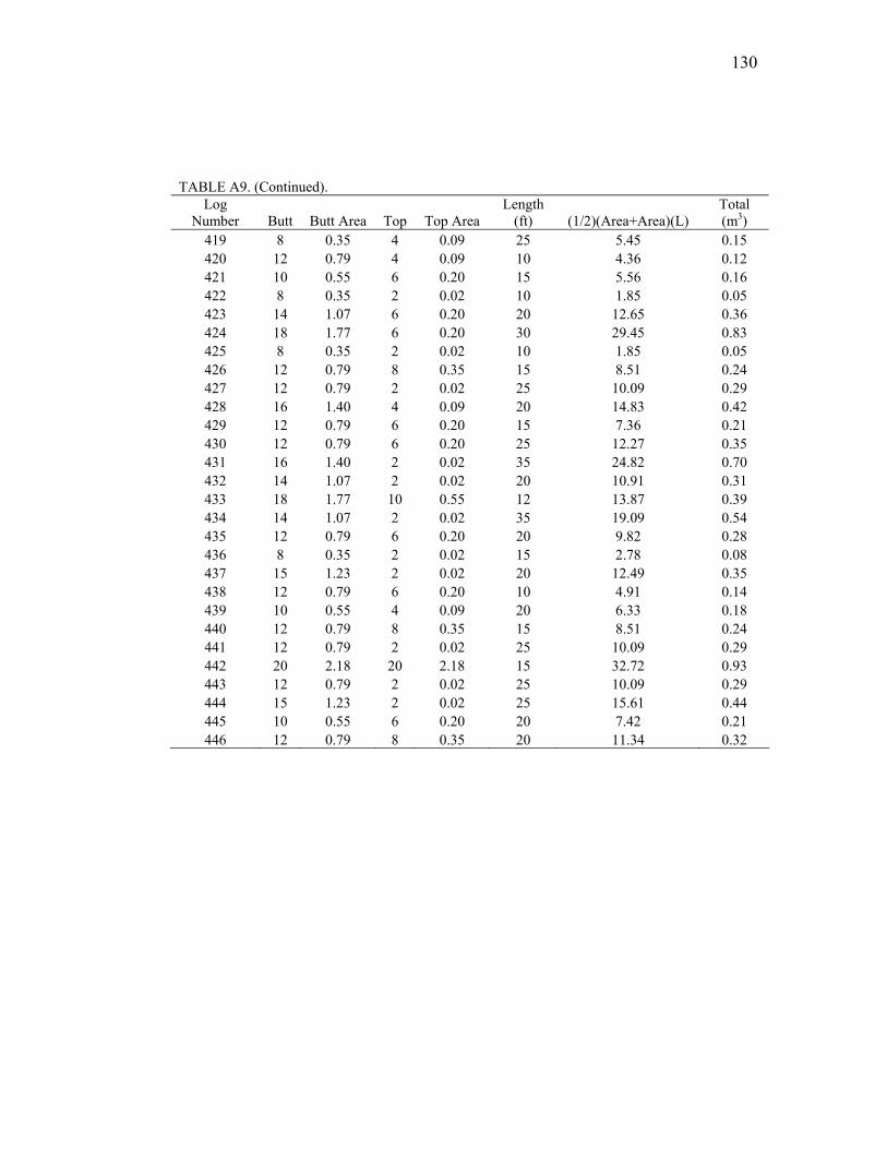
130
TABLE A9. (Continued).
Log Number Butt Butt Area Top Top Area
Length (ft) (1/2)(Area+Area)(L)
Total (m3)
419 8 0.35 4 0.09 25 5.45 0.15 420 12 0.79 4 0.09 10 4.36 0.12 421 10 0.55 6 0.20 15 5.56 0.16 422 8 0.35 2 0.02 10 1.85 0.05 423 14 1.07 6 0.20 20 12.65 0.36 424 18 1.77 6 0.20 30 29.45 0.83 425 8 0.35 2 0.02 10 1.85 0.05 426 12 0.79 8 0.35 15 8.51 0.24 427 12 0.79 2 0.02 25 10.09 0.29 428 16 1.40 4 0.09 20 14.83 0.42 429 12 0.79 6 0.20 15 7.36 0.21 430 12 0.79 6 0.20 25 12.27 0.35 431 16 1.40 2 0.02 35 24.82 0.70 432 14 1.07 2 0.02 20 10.91 0.31 433 18 1.77 10 0.55 12 13.87 0.39 434 14 1.07 2 0.02 35 19.09 0.54 435 12 0.79 6 0.20 20 9.82 0.28 436 8 0.35 2 0.02 15 2.78 0.08 437 15 1.23 2 0.02 20 12.49 0.35 438 12 0.79 6 0.20 10 4.91 0.14 439 10 0.55 4 0.09 20 6.33 0.18 440 12 0.79 8 0.35 15 8.51 0.24 441 12 0.79 2 0.02 25 10.09 0.29 442 20 2.18 20 2.18 15 32.72 0.93 443 12 0.79 2 0.02 25 10.09 0.29 444 15 1.23 2 0.02 25 15.61 0.44 445 10 0.55 6 0.20 20 7.42 0.21 446 12 0.79 8 0.35 20 11.34 0.32

131
TABLE A10. Deweyville Smalian's Formula for finding log volume
Log Number Butt Butt Area Top Top Area
Length (ft) (1/2)(Area+Area)(L)
Total (m3)
101 12 0.79 13.5 0.99 30 26.69 0.76 102 14.1 1.08 11.3 0.70 15 13.36 0.38 103 12 0.79 9 0.44 10 6.14 0.17 104 10 0.55 6 0.20 11 4.08 0.12 105 8.2 0.37 3 0.05 30 6.24 0.18 106 8.9 0.43 5 0.14 40 11.37 0.32 107 5 0.14 5 0.14 8 1.09 0.03 108 14 1.07 12 0.79 15 13.91 0.39 109 14 1.07 12 0.79 15 13.91 0.39 110 15 1.23 8 0.35 20 15.76 0.45 111 6 0.20 2 0.02 25 2.73 0.08 112 6 0.20 2 0.02 20 2.18 0.06 113 7 0.27 2 0.02 40 5.78 0.16 114 9 0.44 4 0.09 25 6.61 0.19 115 27.2 4.04 18 1.77 50 145.05 4.11 116 9 0.44 3 0.05 30 7.36 0.21 117 17 1.58 15 1.23 20 28.03 0.79 118 10 0.55 8 0.35 7 3.13 0.09 119 6 0.20 3 0.05 20 2.45 0.07 120 14.4 1.13 10 0.55 12 10.06 0.28 121 7.3 0.29 4 0.09 20 3.78 0.11 122 10.6 0.61 5 0.14 25 9.36 0.27 123 10 0.55 10 0.55 8 4.36 0.12 124 9.4 0.48 4 0.09 11 3.13 0.09 125 8 0.35 2 0.02 15 2.78 0.08 126 10 0.55 10 0.55 20 10.91 0.31 127 14 1.07 10 0.55 20 16.14 0.46 128 17 1.58 10 0.55 50 53.04 1.50 129 5.4 0.16 4 0.09 15 1.85 0.05 130 13.3 0.96 2 0.02 20 9.87 0.28 131 15 1.23 10 0.55 20 17.73 0.50 132 18 1.77 7 0.27 40 40.69 1.15 133 12 0.79 5 0.14 20 9.22 0.26 134 15 1.23 6 0.20 55 39.15 1.11 135 9 0.44 2 0.02 40 9.27 0.26 136 12 0.79 5.5 0.16 40 19.01 0.54 137 8 0.35 4 0.09 12 2.62 0.07 138 12 0.79 11 0.66 30 21.68 0.61

132
TABLE A10. (Continued).
Log Number Butt Butt Area Top Top Area
Length (ft) (1/2)(Area+Area)(L)
Total (m3)
139 20.6 2.31 8 0.35 40 53.27 1.51 140 12.3 0.83 12 0.79 6.5 5.23 0.15 141 15 1.23 10.4 0.59 25 22.71 0.64 142 14 1.07 3 0.05 20 11.18 0.32 143 12 0.79 6 0.20 15 7.36 0.21 144 4 0.09 8 0.35 30 6.54 0.19 145 7 0.27 4.2 0.10 25 4.54 0.13 146 10 0.55 2 0.02 35 9.93 0.28 147 4 0.09 8 0.35 15 3.27 0.09 148 4 0.09 8 0.35 10 2.18 0.06 149 11 0.66 2 0.02 20 6.82 0.19 151 5 0.14 5 0.14 10 1.36 0.04 232 8 0.35 6 0.20 8 2.18 0.06 233 12 0.79 4 0.09 45 19.63 0.56 234 12 0.79 4 0.09 50 21.82 0.62 235 10 0.55 6 0.20 20 7.42 0.21 236 8 0.35 6 0.20 20 5.45 0.15 237 6 0.20 4 0.09 15 2.13 0.06 238 7 0.27 2 0.02 45 6.50 0.18 239 6 0.20 2 0.02 15 1.64 0.05 240 6 0.20 4 0.09 15 2.13 0.06 241 13 0.92 13 0.92 12 11.06 0.31 242 10 0.55 4 0.09 12 3.80 0.11 243 10 0.55 8 0.35 15 6.71 0.19 244 6 0.20 4 0.09 20 2.84 0.08 245 13 0.92 8 0.35 20 12.71 0.36 246 16 1.40 12 0.79 40 43.63 1.24 247 6 0.20 6 0.20 20 3.93 0.11 248 12 0.79 2 0.02 20 8.07 0.23 249 10 0.55 5 0.14 15 5.11 0.14 250 10 0.55 2 0.02 25 7.09 0.20 251 14 1.07 6 0.20 15 9.49 0.27 252 8 0.35 6 0.20 25 6.82 0.19 253 12 0.79 8 0.35 8 4.54 0.13 254 8 0.35 5 0.14 20 4.85 0.14 255 12 0.79 2 0.02 50 20.18 0.57 256 10 0.55 6 0.20 15 5.56 0.16 257 8 0.35 4 0.09 25 5.45 0.15 258 8 0.35 2 0.02 25 4.64 0.13

133
TABLE A10. (Continued). Log
Number Butt Butt Area Top Top Area Length
(ft) (1/2)(Area+Area)(L) Total (m3)
259 16 1.40 2 0.02 45 31.91 0.90 260 8 0.35 4 0.09 20 4.36 0.12 261 8 0.35 3 0.05 20 3.98 0.11 262 12 0.79 4 0.09 25 10.91 0.31 263 13 0.92 3 0.05 25 12.14 0.34 264 16 1.40 2 0.02 50 35.45 1.00 265 20 2.18 10 0.55 15 20.45 0.58 266 13 0.92 12 0.79 30 25.61 0.73 267 8 0.35 2 0.02 40 7.42 0.21 268 20 2.18 18 1.77 15 29.62 0.84 269 10 0.55 8 0.35 15 6.71 0.19 270 12 0.79 8 0.35 25 14.18 0.40 271 20 2.18 2 0.02 30 33.05 0.94 272 18 1.77 6 0.20 15 14.73 0.42 273 12 0.79 12 0.79 30 23.56 0.67 274 14 1.07 8 0.35 40 28.36 0.80 275 22 2.64 8 0.35 40 59.78 1.69 276 10 0.55 2 0.02 25 7.09 0.20 277 13 0.92 10 0.55 25 18.34 0.52 278 6 0.20 6 0.20 15 2.95 0.08 279 11 0.66 9 0.44 20 11.02 0.31 280 14 1.07 8 0.35 25 17.73 0.50 281 16 1.40 8 0.35 35 30.54 0.86 282 16 1.40 2 0.02 30 21.27 0.60 283 16 1.40 8 0.35 30 26.18 0.74 284 7 0.27 4 0.09 32 5.67 0.16 285 10 0.55 2 0.02 30 8.51 0.24 286 10 0.55 2 0.02 30 8.51 0.24 287 12 0.79 10 0.55 5 3.33 0.09 288 12 0.79 3 0.05 35 14.60 0.41 289 12 0.79 3 0.05 50 20.86 0.59 290 12 0.79 2 0.02 70 28.25 0.80 291 26 3.69 10 0.55 35 74.07 2.10 292 14 1.07 9 0.44 25 18.88 0.53 293 19 1.97 10 0.55 35 44.00 1.25 294 15 1.23 11 0.66 20 18.87 0.53 295 6 0.20 2 0.02 20 2.18 0.06 296 15 1.23 6 0.20 18 12.81 0.36 297 11 0.66 11 0.66 7 4.62 0.13 298 9 0.44 9 0.44 10 4.42 0.13 299 8 0.35 2 0.02 20 3.71 0.11 300 8 0.35 2 0.02 25 4.64 0.13

134
TABLE A11. Frequency counts for Contingency Tests for branch presence vs. position categories.
Categories Burkeville Bon Wier Deweyville Southern
Yes, Fallen Tree 21 0 38 18
No, Fallen Tree 11 0 12 5
Yes, Jam 8 8 3 3
No, Jam 26 4 35 30
Yes, Individual 12 26 8 1
No, Individual 15 57 23 8

135
TABLE A12. Frequency counts for Contingency Tests for degree of decay vs. position categories. Categories Burkeville Bon Wier Deweyville Southern
1, Fallen Tree 7 0 14 4 1, Jam 0 4 1 0 1, Individual 0 11 2 1 2, Fallen Tree 11 0 19 7 2, Jam 5 3 3 2 2, Individual 2 11 2 0 3, Fallen Tree 7 0 13 8 3, Jam 24 4 16 8 3, Individual 17 37 17 2 4, Fallen Tree 5 0 4 3 4, Jam 5 1 17 22 4, Individual 7 18 10 14 5, Fallen Tree 2 0 0 1 5, Jam 0 0 1 1 5, Individual 1 6 0 2

136
TABLE A13. Frequency counts for Contingency Tests for bank orientation vs. position categories.
Categories Burkeville Bon Wier Deweyville Southern
90, Fallen Tree 9 0 24 19
90, Individual 6 27 19 5
90, Jam 13 4 11 19
0, Fallen Tree 19 0 17 1
0, Individual 19 35 3 1
0, Jam 18 6 15 7
180, Fallen Tree 4 0 9 3
180, Individual 2 21 8 3
180, Jam 3 1 9 7
TABLE A14. Frequency counts for Contingency Tests for bank orientation vs. stage contact categories.
Categories Burkeville Bon Wier Deweyville Southern
90, 1 24 29 31 40 90, 2 2 2 17 2 90, 3 1 0 5 2 90, 4 1 0 1 1 0, 1 48 39 27 8 0, 2 8 1 6 0 0, 3 0 1 0 0 0, 4 0 0 2 1
180, 1 4 22 20 10 180, 2 4 0 2 1 180, 3 1 0 4 1 180, 4 0 0 0 1

137
TABLE A15. Frequency counts for Contingency Tests for bank orientation vs. stage contact categories. Categories Burkeville Bon Wier Deweyville Southern Fallen Tree, 1 18 0 34 20 Fallen Tree, 2 11 0 7 2 Fallen Tree, 3 2 0 7 1 Fallen Tree, 4 1 0 2 0 Individual, 1 27 79 1 5 Individual, 2 0 3 1 0 Individual, 3 0 1 2 1 Individual, 4 0 0 2 3 Jam, 1 31 12 27 31 Jam, 2 3 0 8 1 Jam, 3 0 0 0 1 Jam, 4 0 0 3 0
TABLE A16. Frequency counts for Contingency Tests for root wad vs. position categories.
Categories Burkeville Bon Wier Deweyville Southern
Yes, Fallen Tree 17 0 40 29
No, Fallen Tree 6 0 3 3
Yes, Individual 1 34 8 10
No, Individual 8 12 20 5
Yes, Jam 2 9 14 14
No, Jam 30 2 18 16

138
TABLE A17. Frequency counts for Contingency Tests for root wad vs. stage contact categories.
Categories Burkeville Bon Wier Deweyville Southern
Yes, 1 37 42 41 18
No, 1 23 12 21 39
Yes, 2 13 1 13 1
No, 2 1 1 12 2
Yes, 3 2 0 6 1
No, 3 0 1 3 2
Yes, 4 1 0 2 0
No, 4 0 0 5 1
TABLE A18. Frequency counts for Contingency Tests for branch presence vs. root wad categories.
Categories Burkeville Bon Wier Deweyville Southern
Yes, Yes 33 22 36 17
Yes, No 1 4 4 4
No, Yes 20 21 26 3
No, No 23 10 37 42
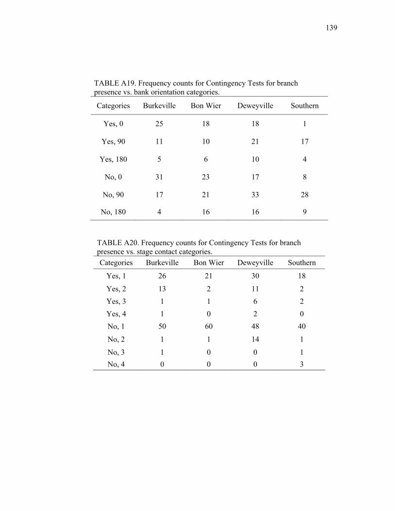
139
TABLE A19. Frequency counts for Contingency Tests for branch presence vs. bank orientation categories.
Categories Burkeville Bon Wier Deweyville Southern
Yes, 0 25 18 18 1
Yes, 90 11 10 21 17
Yes, 180 5 6 10 4
No, 0 31 23 17 8
No, 90 17 21 33 28
No, 180 4 16 16 9
TABLE A20. Frequency counts for Contingency Tests for branch presence vs. stage contact categories. Categories Burkeville Bon Wier Deweyville Southern
Yes, 1 26 21 30 18
Yes, 2 13 2 11 2 Yes, 3 1 1 6 2 Yes, 4 1 0 2 0 No, 1 50 60 48 40
No, 2 1 1 14 1
No, 3 1 0 0 1 No, 4 0 0 0 3

140
TABLE A21. Frequency counts for Contingency Tests for degree of decay vs. branch presence categories. Categories Burkeville Bon Wier Deweyville Southern
1, Yes 7 13 17 5
2, Yes 15 12 17 8
3, Yes 17 7 15 5
4, Yes 2 1 0 4
5, Yes 0 1 0 0
1, No 0 2 0 0
2, No 3 2 7 1
3, No 31 34 31 14
4, No 15 18 31 26
5, No 3 5 1 4

141
TABLE A22. Frequency counts for Contingency Tests for degree of decay vs. stage contact categories. Categories Burkeville Bon Wier Deweyville Southern
1, 1 0 12 8 2 1, 2 5 2 7 1 1, 3 1 1 0 2 1, 4 1 0 2 0 2, 1 13 14 18 8 2, 2 5 0 2 1 2, 3 0 0 4 0 2, 4 0 0 0 0 3, 1 43 40 29 18 3, 2 4 1 11 0 3, 3 1 0 4 0 3, 4 0 0 2 1 4, 1 17 19 23 26 4, 2 0 0 5 1 4, 3 0 0 1 1 4, 4 0 0 2 2 5, 1 3 6 0 4 5, 2 0 0 0 0 5, 3 0 0 0 0 5, 4 0 0 1 0

142
TABLE A23. Frequency counts for Contingency Tests for degree of decay vs. root wad categories. Categories Burkeville Bon Wier Deweyville Southern
1, Yes 6 11 16 4
1, No 1 2 0 1
2, Yes 16 10 20 6
2, No 1 1 1 3
3, Yes 21 17 17 5
3, No 17 8 21 14
4, Yes 8 2 9 3
4, No 5 2 18 26
5, Yes 2 3 0 2 5, No 0 1 1 2
TABLE A24. Frequency counts for Contingency Tests for orientation vs. root wad categories.
Categories Burkeville Bon Wier Deweyville Southern
90, No 6 5 20 29
90, Yes 17 17 27 15
180, No 1 2 11 9
180, Yes 7 9 13 4
0, No 17 6 6 8
0, Yes 29 17 22 1

143

TABLE A25. Chi-Square values from the Two-Way Contingency Table analysis of the Degree of Decay category.
Degree of Decay Sites
Burkeville Deweyville Southern Bon Wier 1 1.42 0.64 1.05 1.31 2 0.21 0.53 0.60 0.38 3 2.46 0.18 2.67 0.09 4 2.10 0.00 9.17 1.29 5 0.07 2.68 0.89 1.68
TABLE A26. Chi-Square values from the Two-Way Contingency Table analysis of the Bank Orientation category.
Bank Orientation Sites
Burkeville Deweyville Southern Bon Wier 0 11.78 1.82 10.77 0.72 90 3.51 0.46 9.27 2.13 180 4.23 0.80 0.00 0.97
TABLE A27. Chi-Square values from the Two-Way Contingency Table analysis of the Stage Contact category.
Stage Contact Sites Burkeville Deweyville Southern Bon Wier 1 0.01 3.52 0.25 2.56 2 0.71 7.97 3.18 6.22 3 0.80 3.74 0.04 2.07 4 1.10 3.50 0.54 2.79

TABLE A28. Chi-Square values from the Two-Way Contingency Table analysis of the Position category.
Position Sites Burkeville Deweyville Southern Bon Wier
Fallen Tree 1.23 7.91 1.32 26.89 Individual 2.87 5.90 12.19 52.71
Jam 0.74 0.01 8.14 10.77 TABLE A29. Chi-Square values from the Two-Way Contingency Table analysis of the Origin category.
Origin Sites Burkeville Deweyville Southern Bon Wier
Local 6.45 4.75 1.04 2.94 Upstream 15.99 11.78 2.58 7.30
TABLE A30. Chi-Square values from the Two-Way Contingency Table analysis of the Branch Presence category.
Branch Presence Sites
Burkeville Deweyville Southern Bon Wier Yes 0.61 0.14 0.66 0.26 No 0.39 0.09 0.42 0.16
TABLE A31. Chi-Square values from the Two-Way Contingency Table analysis of the Root Wad Presence category.
Root Wad Presence Sites
Burkeville Deweyville Southern Bon Wier Yes 1.33 0.04 9.09 2.70 No 1.90 0.05 12.94 3.85

TABLE A32. Chi-Square values from the Two-Way Contingency Table analysis of the Potential Source category.
Potential Source Sites
Burkeville Deweyville Southern Bon Wier Bank cut 9.23 2.50 14.31 1.53 Windsnap 3.08 6.85 0.46 0.02 Windthrow 12.30 0.95 33.65 2.95