The determinants of future economic

growth

Sabbatical programme report

Fernando Cantu∗

UN-ESCWA

20 February 2016

Abstract

The present document describes the main activities undertakenas part of the Sabbatical Programme 2015. This is a joint projectbetween the staff member and Prof. Havard Hegre of the Peace Re-search Institute Oslo (PRIO). The main objective of the research is todefine, set-up and estimate a structural macroeconomic model to cal-culate long-term economic forecasts for all the countries in the world.The distinctive feature of such a model is that it will consider the en-dogenous relationship between economic growth and internal armedconflict. As a result, it can be used to estimate the long-term costsof conflict on development and, ultimately, on the lives of the affectedpopulation.

∗E-mail: cantu@un.org

1

1 Introduction

Long-term macroeconomic forecasts are useful to study the long-term (poten-

tial) growth path of the economy, which can feed into shorter-term cycles of

the economic cycle in order to estimate output gaps. They are also essential

to study phenomena, such as demographic trends or the impact of climate

change, which only have a modest impact in the short-term but whose effects

become dominant in the long-term. For these reasons, many institutions at

the national and international level place considerable efforts into calculating

long-term macroeconomic forecasts with varying levels of complexity.

Conflict can have disastrous consequences on the population both in the

long and the short term. The violent actions carried out by the warring par-

ties could lead to injuries and battle-related deaths, increased incidence of

transmittable diseases, forced displacement, lower participation in education,

destruction of productive infrastructure, reduction in international trade and

financial flows, increased perception of risk, and many others consequences.

All these factors can damage short-term development prospects. In addition,

there is a long-term effect on the economy and the livelihood of the popu-

lation through permanent damage to the economic structure, long-lasting

perception of risk, and a generalized decrease in the quantity and quality

of human and physical capital. In addition, the risk of relapse can remain

high for an extended period, particularly in conditions of economic decline,

increasing the chances of falling into “conflict traps”. Finally, conflicts do

not occur in isolation from the rest of the world and they can also exert an

influence to neighboring countries, both in terms of economic spillover effects

and the possibility of conflict contagion.

Long-term economic forecasts that ignore the possibility of falling into

2

armed conflict can severely overestimate future growth paths.1 Recent exer-

cises have tried to take into account the likelihood of conflict when construct-

ing long-term economic forecasts. A prime example is Hegre et al. (2013),

which generates joint conflict-growth paths over the horizon 2011-2050 for

a large group of countries and uses them to estimate the long-term costs of

conflict on the economies.

One of the weakness of this literature is that it generally neglects the

endogenous relationship between conflict and economic growth. Conflict

studies have time and again identified economic decline as a determinant

of conflict. To see this, it suffices to document that the overwhelming ma-

jority of conflicts since the end of World War II have taken place in low-

or mid-low-income countries. However, as discussed above, there is also vast

evidence that conflict has serious repercussions in terms of economic activity.

Disentangling such a two-way relationship required special identification and

statistical techniques that have been mostly absent from previous studies.

These can lead to a significant estimation bias, which can become specially

problematic when attempting to extend the forecast over many years.

I have undertaken a research project together with Prof. Havard Hegre of

the Peace Research Institute Oslo (PRIO) with the objectives of calculating

long-term macroeconomic forecasts that explicitly consider the endogenous

link with conflict. The project has then three main components: (i) set-up

a structural macroeconomic model that can be used to estimate the main

determinants of growth over the long term; (ii) modify the estimation and

identification of the preceding model so that it takes into account the endoge-

nous link with conflict; and, (iii) calculate long-term forecasts for economic

1To illustrate this, consider the prospects of the Syrian economy calculated in 2010through a long-term economic model that ignores the possibility of conflict onset. Theresulting estimates would be far too high given the disastrous short- and long-term con-sequences of the ongoing crisis.

3

growth and conflict for a large cross-section of conflict.

This report describes the work accomplished so far in this research project.

Note that this is a long-term project whose duration extends beyond the sab-

batical programme. Indeed, it is still ongoing, with frequent updates between

Prof. Hegre and myself.

As a final note, a few words on some limitations of scope for this study.

It only incorporates internal armed conflict, according to the definition used

in the PRIO/UCDP database.2 This is because the vast majority of armed

conflicts since the end of World War II are internal and this trend is expected

to continue. Also, internal conflicts usually last longer, have a more more

harmful impact on the people and the economys and have higher risk of re-

lapse than external conflict. In terms of geographic coverage, all independent

countries of the world with available information will be considered. Finally,

the forecast horizon is from 2014 (or earlier, if data is incomplete) up to 2100.

2 Construction of economic growth forecasts:

a walkthrough

Through a combination of the approaches described in Johansson et al. (2012)

and Foure et al. (2012), we define a production function based on three pro-

duction factors: capital, labour and energy. However, while capital and

labour could be considered as substitutes, this cannot extend to energy. To

account for this low substitution rate between energy and capital/labour,

a nested production function is used: a Constant Elasticity of Substitution

(CES) function with two factor groups: energy and a Cobb-Douglas combi-

2See http://www.prio.org/Data/Armed-Conflict/UCDP-PRIO.

4

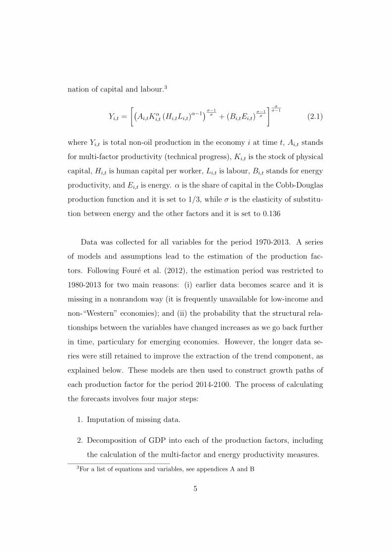
nation of capital and labour.3

Yi,t =

[(Ai,tK

αi,t (Hi,tLi,t)

α−1)σ−1σ + (Bi,tEi,t)

σ−1σ

] σσ−1

(2.1)

where Yi,t is total non-oil production in the economy i at time t, Ai,t stands

for multi-factor productivity (technical progress), Ki,t is the stock of physical

capital, Hi,t is human capital per worker, Li,t is labour, Bi,t stands for energy

productivity, and Ei,t is energy. α is the share of capital in the Cobb-Douglas

production function and it is set to 1/3, while σ is the elasticity of substitu-

tion between energy and the other factors and it is set to 0.136

Data was collected for all variables for the period 1970-2013. A series

of models and assumptions lead to the estimation of the production fac-

tors. Following Foure et al. (2012), the estimation period was restricted to

1980-2013 for two main reasons: (i) earlier data becomes scarce and it is

missing in a nonrandom way (it is frequently unavailable for low-income and

non-“Western” economies); and (ii) the probability that the structural rela-

tionships between the variables have changed increases as we go back further

in time, particulary for emerging economies. However, the longer data se-

ries were still retained to improve the extraction of the trend component, as

explained below. These models are then used to construct growth paths of

each production factor for the period 2014-2100. The process of calculating

the forecasts involves four major steps:

1. Imputation of missing data.

2. Decomposition of GDP into each of the production factors, including

the calculation of the multi-factor and energy productivity measures.

3For a list of equations and variables, see appendices A and B

5

3. Isolation of the trend component of the variables included in the pro-

duction function. This will help to better estimate their evolution and

generate forecasts that do not depend on the stage of the cycle that

the countries are traversing at the end of the observed period.

4. Construction of forecasts for the production factors and aggregation

into GDP forecasts over the horizon 2100.

Note that, as a consequence of the third step, the forecasts are constructed

only for the trend component of GDP.

2.1 Data sources and imputations

Details on the main sources of data used and the method to impute missing

data, if any, are detailed below. All independent countries of the world were

considered. Data was collected for the period 1970-2013.

• POP is total population from the United Nation’s World Population

Prospects 2012 Revision. The data is complete (with the exception

of countries with a population of 500 000 or less, which are excluded

altogether), so no imputation was performed.

• WAPOP is working-age population, defined as the population aged 15

years and more for the purpose of this paper. Obtained from the same

source as POP .

• Y is defined as constant GDP at 2011 PPP USD from the World’s Bank

World Development Indicators (WDIs). Missing data are imputed by

applying rates of change from Penn World Tables (PWTs) version 8.1.

Argentina and Syria are missing completely from the WDIs, so they

were obained from the IMF’s World Economic Outlook (WEO) April

6

2015 database, which follows the same base year than the WDIs. (0-

4-Complete GDP.R)

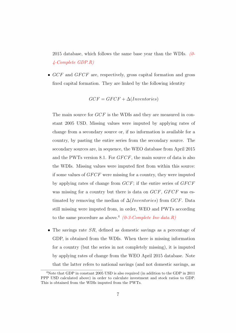
• GCF and GFCF are, respectively, gross capital formation and gross

fixed capital formation. They are linked by the following identity

GCF = GFCF + ∆(Inventories)

The main source for GCF is the WDIs and they are measured in con-

stant 2005 USD. Missing values were imputed by applying rates of

change from a secondary source or, if no information is available for a

country, by pasting the entire series from the secondary source. The

secondary sources are, in sequence, the WEO database from April 2015

and the PWTs version 8.1. For GFCF , the main source of data is also

the WDIs. Missing values were imputed first from within this source:

if some values of GFCF were missing for a country, they were imputed

by applying rates of change from GCF ; if the entire series of GFCF

was missing for a country but there is data on GCF , GFCF was es-

timated by removing the median of ∆(Inventories) from GCF . Data

still missing were imputed from, in order, WEO and PWTs according

to the same procedure as above.4 (0-3-Complete Inv data.R)

• The savings rate SR, defined as domestic savings as a percentage of

GDP, is obtained from the WDIs. When there is missing information

for a country (but the series in not completely missing), it is imputed

by applying rates of change from the WEO April 2015 database. Note

that the latter refers to national savings (and not domestic savings, as

4Note that GDP in constant 2005 USD is also required (in addition to the GDP in 2011PPP USD calculated above) in order to calculate investment and stock ratios to GDP.This is obtained from the WDIs imputed from the PWTs.

7

in the WDIs). Although they may still be a reasonable approximation,

only rates of change are used (and never the series in levels). (0-5-

Complete SR.R)

• The unemployment rate UR is obtained from the WDIs, which reports

International Labour Organization (ILO) estimates. Missing data is

imputed from the WEO April 2015 database. (0-6-Complete UR.R)

• Labour force participation rate of the working-age population LFPR15+

is obtained from ILO Labour Statistics. This database is complete and

no imputation is applied. This variables is also available divided by

sex-age group.

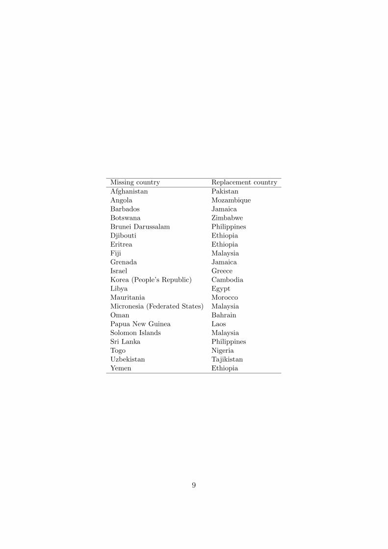
• Education data are summarized through three variables: Secondary

school attainment of the adult (25+) population SecAtt25+, post-secondary

school attainment of the adult population PostSecAtt25+, and mean

years of schooling of the adult population S25+. All are obtained

from the International Institute for Applied Systems Analysis (IIASA)

database, which were aggregated to the desired age group. Some coun-

tries are missing from the database, and they are completed through

data from “proximate” countries in the same region, as identified by

PRIO (with the exception of Grenada, Israel and Micronesia, which

were not considered in PRIO’s processing, and were replaced with data

from Jamaica, Greece and Malaysia, respectively). For some coun-

tries, the entire series is missing and it is filled with the replacement

country; for others, only the data from 2010 and onwards is available,

so rates of change of the replacement country are applied backwards.

The concerned countries along with the replacement countries are in-

cluded below. The education variables are available from the source in

8

Missing country Replacement country

Afghanistan PakistanAngola MozambiqueBarbados JamaicaBotswana ZimbabweBrunei Darussalam PhilippinesDjibouti EthiopiaEritrea EthiopiaFiji MalaysiaGrenada JamaicaIsrael GreeceKorea (People’s Republic) CambodiaLibya EgyptMauritania MoroccoMicronesia (Federated States) MalaysiaOman BahrainPapua New Guinea LaosSolomon Islands MalaysiaSri Lanka PhilippinesTogo NigeriaUzbekistan TajikistanYemen Ethiopia

9

five-year intervals. When required, they are converted into yearly se-

ries through linear interpolation. (0-7-Preprocessing ed attainment.R,

0-8-Complete education.R)

• Oil rents as percentage of GDP are required to divide GDP into oil pro-

duction and non-oil production. These are obtained from the WDIs.

Some missing data are imputed with zero when it is clear that the

country, at the concerned period, was not producing oil (verified from

the United States Energy Information Agency (EIA) and various other

sources). Missing data are then imputed by applying rates of change

from a calculated series of oil rents as percentage of GDP, calculated

by multiplying the estimated volume of oil production times the inter-

national price of oil (obtained from the IMF) and dividing by current

GDP.5 In order to maintain consistency, imputed values of oil produc-

tion cannot exceed 90% of GDP. (0-9-Complete oil rents data.R)

• E, energy as a production factor, is obtained from the variable “energy

use (kg of oil equivalent per capita)” from the WDIs. It is transformed

into total energy use by multiplying by POP . This is further trans-

formed into barrels of oil equivalent (1000 kilos of oil equivalent =

6.84357 barrels of oil equivalent). Missing data are imputed by apply-

ing rates of change from energy consumption obtained from EIA. Since

the series are not exactly the same, when no information at all is avail-

able for a country from the WDIs, it is imputed from the EIA through

the estimated coefficients of a linear regression model. (0-10-Complete

energy consumption.R)

5Current GDP in USD is required for this. This is obtained from the WDIs with missingvalues imputed by applying rates of change from, in order, WEO April 2015 database andUN Data.

10

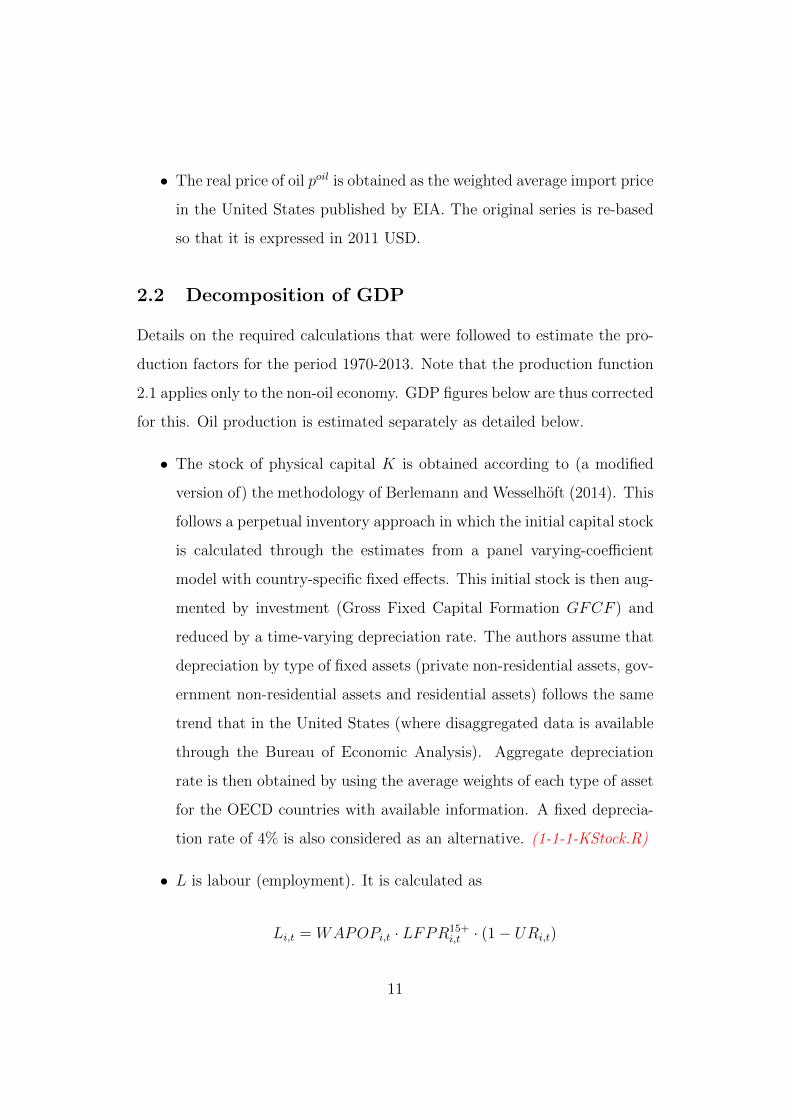
• The real price of oil poil is obtained as the weighted average import price

in the United States published by EIA. The original series is re-based

so that it is expressed in 2011 USD.

2.2 Decomposition of GDP

Details on the required calculations that were followed to estimate the pro-

duction factors for the period 1970-2013. Note that the production function

2.1 applies only to the non-oil economy. GDP figures below are thus corrected

for this. Oil production is estimated separately as detailed below.

• The stock of physical capital K is obtained according to (a modified

version of) the methodology of Berlemann and Wesselhoft (2014). This

follows a perpetual inventory approach in which the initial capital stock

is calculated through the estimates from a panel varying-coefficient

model with country-specific fixed effects. This initial stock is then aug-

mented by investment (Gross Fixed Capital Formation GFCF ) and

reduced by a time-varying depreciation rate. The authors assume that

depreciation by type of fixed assets (private non-residential assets, gov-

ernment non-residential assets and residential assets) follows the same

trend that in the United States (where disaggregated data is available

through the Bureau of Economic Analysis). Aggregate depreciation

rate is then obtained by using the average weights of each type of asset

for the OECD countries with available information. A fixed deprecia-

tion rate of 4% is also considered as an alternative. (1-1-1-KStock.R)

• L is labour (employment). It is calculated as

Li,t = WAPOPi,t · LFPR15+i,t · (1− URi,t)

11

(1-1-2-Labour.R)

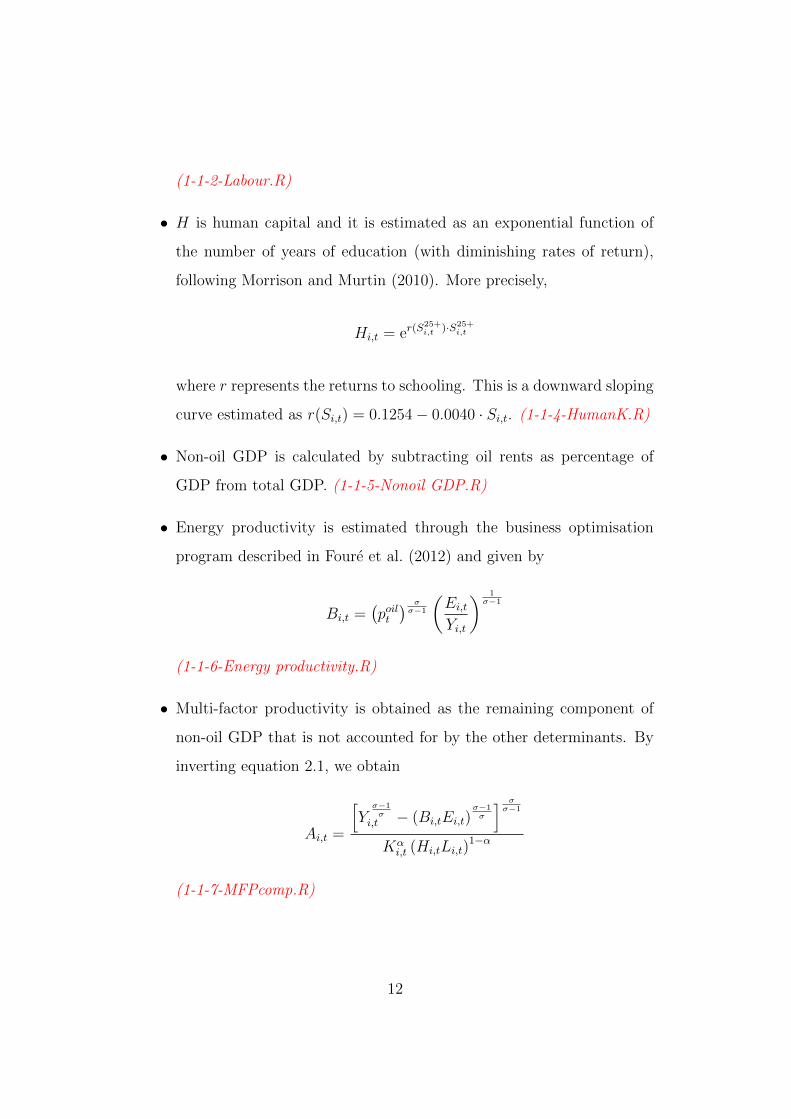
• H is human capital and it is estimated as an exponential function of

the number of years of education (with diminishing rates of return),

following Morrison and Murtin (2010). More precisely,

Hi,t = er(S25+i,t )·S25+

i,t

where r represents the returns to schooling. This is a downward sloping

curve estimated as r(Si,t) = 0.1254− 0.0040 · Si,t. (1-1-4-HumanK.R)

• Non-oil GDP is calculated by subtracting oil rents as percentage of

GDP from total GDP. (1-1-5-Nonoil GDP.R)

• Energy productivity is estimated through the business optimisation

program described in Foure et al. (2012) and given by

Bi,t =(poilt) σσ−1

(Ei,tYi,t

) 1σ−1

(1-1-6-Energy productivity.R)

• Multi-factor productivity is obtained as the remaining component of

non-oil GDP that is not accounted for by the other determinants. By

inverting equation 2.1, we obtain

Ai,t =

[Y

σ−1σ

i,t − (Bi,tEi,t)σ−1σ

] σσ−1

Kαi,t (Hi,tLi,t)

1−α

(1-1-7-MFPcomp.R)

12

2.3 Isolation of trend components

All economic time series can be decomposed into at least three elements:

trend component, cycle component and irregular component. If a variable’s

frequency is infra-annual, a fourth element could be considered: the seasonal

component. The usefulness of isolating the trend component of the variables

in the production function is twofold: it allows a better estimation of the

relationship between the variables and their determinants, and it allows to

generate forecasts that do not depend on the stage of the cycle at the end of

the observational period and the beginning of the forecast period. This sec-

tion described how these trend components were calculated for the variables

where this is required.

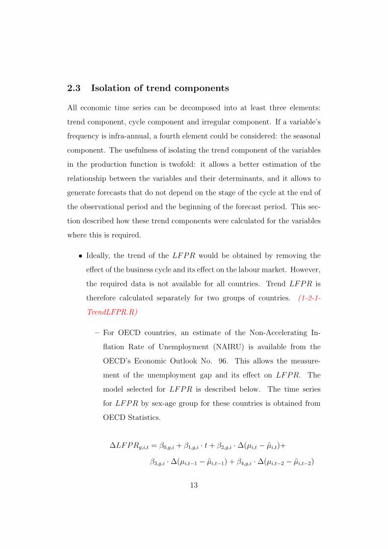
• Ideally, the trend of the LFPR would be obtained by removing the

effect of the business cycle and its effect on the labour market. However,

the required data is not available for all countries. Trend LFPR is

therefore calculated separately for two groups of countries. (1-2-1-

TrendLFPR.R)

– For OECD countries, an estimate of the Non-Accelerating In-

flation Rate of Unemployment (NAIRU) is available from the

OECD’s Economic Outlook No. 96. This allows the measure-

ment of the unemployment gap and its effect on LFPR. The

model selected for LFPR is described below. The time series

for LFPR by sex-age group for these countries is obtained from

OECD Statistics.

∆LFPRg,i,t = β0,g,i + β1,g,i · t+ β2,g,i ·∆(µi,t − µi,t)+

β3,g,i ·∆(µi,t−1 − µi,t−1) + β4,g,i ·∆(µi,t−2 − µi,t−2)

13

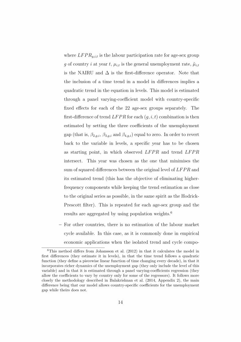
where LFPRg,i,t is the labour participation rate for age-sex group

g of country i at year t, µi,t is the general unemployment rate, µi,t

is the NAIRU and ∆ is the first-difference operator. Note that

the inclusion of a time trend in a model in differences implies a

quadratic trend in the equation in levels. This model is estimated

through a panel varying-coefficient model with country-specific

fixed effects for each of the 22 age-sex groups separately. The

first-difference of trend LFPR for each (g, i, t) combination is then

estimated by setting the three coefficients of the unemployment

gap (that is, β2,g,i, β3,g,i and β4,g,i) equal to zero. In order to revert

back to the variable in levels, a specific year has to be chosen

as starting point, in which observed LFPR and trend LFPR

intersect. This year was chosen as the one that minimises the

sum of squared differences between the original level of LFPR and

its estimated trend (this has the objective of eliminating higher-

frequency components while keeping the trend estimation as close

to the original series as possible, in the same spirit as the Hodrick-

Prescott filter). This is repeated for each age-sex group and the

results are aggregated by using population weights.6

– For other countries, there is no estimation of the labour market

cycle available. In this case, as it is commonly done in empirical

economic applications when the isolated trend and cycle compo-

6This method differs from Johansson et al. (2012) in that it calculates the model infirst differences (they estimate it in levels), in that the time trend follows a quadraticfunction (they define a piecewise linear function of time changing every decade), in that itincorporates richer dynamics of the unemployment gap (they only include the level of thisvariable) and in that it is estimated through a panel varying-coefficients regression (theyallow the coefficients to vary by country only for some of the regressors). It follows moreclosely the methodology described in Balakrishnan et al. (2014, Appendix 2), the maindifference being that our model allows country-specific coefficients for the unemploymentgap while theirs does not.

14

nents from a series are required, we apply a corrected Hodrick-

Prescott filter to estimate the trend LFPR for each of the 22 age-

sex groups.7 Although Ravn and Uhlig (2002) suggest a smooth-

ing parameter equal to 6.25 for annual series, we instead choose a

smoothing parameter equal to 100, as done for example in Backus

and Kehoe (1992), in order to achieve a higher degree of smooth-

ness in accordance with the highly-smoothed trend LFPR esti-

mations for the OECD countries described above. The general

LFPR is then obtained by aggregating each of the 22 age-sex

groups through population weights.

• As described above, the estimation of trend unemployment follows a

separate procedure for OECD countries and the rest of the world. For

the former, the NAIRU available from OECD’s Economic Outlook No.

96 is used. For the latter, a corrected Hodrick-Prescott filter with

smoothing parameter 100 is employed. (1-2-2-TrendUNR.R)

• Similarly, the trend of total (oil and non-oil) GDP is obtained from the

OECD for their member countries and through a corrected Hodrick-

Prescott filter with parameter 100 for the rest. (1-2-3-TrendGDP.R)

• For the rest of the relevant variables (K, E, B, A, poil and non-oil

GDP), there are no trend estimations readily available, not even for

a subset of countries. They are all calculated through a corrected

Hodrick-Presctott filter with 100 as smoothing parameter. (1-2-4-

TrendKstock.R, 1-2-5-Trend energy consumption.R, 1-2-6-Trend en-

7Here and in the remaining of the report, the Hodrick-Prescott filter was corrected atthe tail-ends. This because this filter performs poorly at the extremes of the series. Toimprove this, the series is extended at both ends through an automatic ARIMA model.The Hodrick-Prescott filter is then applied to the extended series, but only the originalperiod of observation is maintained.

15

ergy productivity.R, 1.2.7-Trend MFP.R)

• The trend of the average years of schooling and population, required

for example in the modelling of LFPR as a function of educational

attainment, are arguably not required. This because these variables,

obtained from IIASA and UN DESA respectively, are produced through

a model and they are already very smooth. In addition, both educa-

tion and population change very slowly through time and the cyclical

component would be very small in relation to the trend.

2.4 Estimation and forecasting of production factors

and GDP

Each of the elements needed in the production function will be forecasted

individually in order to build up the GDP forecasts. This sections describes

in detail the methodology followed. As justified previously, all relationships

are estimated with data in the period 1980-2013.

• Population forecasts (for POP and WAPOP ) are obtained directly

from the United Nation’s World Population Forecasts 2012 Revision.

• Forecasts for the three variables on educational attainment are obtained

directly from IIASA. These are available at five-year intervals and an-

nual observations are obtained by linear interpolation. These forecasts

are required to calculate human capital and they are also an input in

forecasting labour force participation.

• Unemployment is forecasted by following Johansson et al. (2012). This

16

is done according to the following rule of motion

log µi,t = γ · log µi,t−1 + (1− γ) · log µ∗i

where µi,t is the trend unemployment rate for country i at period t and

µ∗i is the long-term unemployment rate for country i. The criteria to

select the long-term rate of unemployment and the speed of convergence

towards it (γ) are the following. (1-3-1-fcUNR.R)

– For OECD countries, trend unemployment rates converge to their

(country-specific) minimum trend unemployment rate during the

period 2007-2013 at a rate of γ1 = 0.90.

– Non-OECD countries with trend unemployment rate lower than

the OECD average also converge to their (country-specific) min-

imum trend unemployment rate during the period 2007-2013 at

the same rate of γ1 = 0.90.

– Non-OECD countries with trend unemployment rate higher than

the OECD average slowly converge to the long-term rate of un-

employment of the average OECD country at a rate of γ2 = 0.98.

• Labour force participation rates are calculated as a modified version

of International Labour Organisation (2011)’s methodology. This is

done separately for each of 22 age-sex groups: labour force is divided

according to male-female and eleven age intervals (15-19, 20-24, ..., 60-

64 and 65+). For each country i and period t and age-sex group g,

trend LFPR converges to its minimum or maximum rates according

to an exponential time trend. Even if LFPR data is available on a

yearly basis, educational attainment (which would be required later in

17

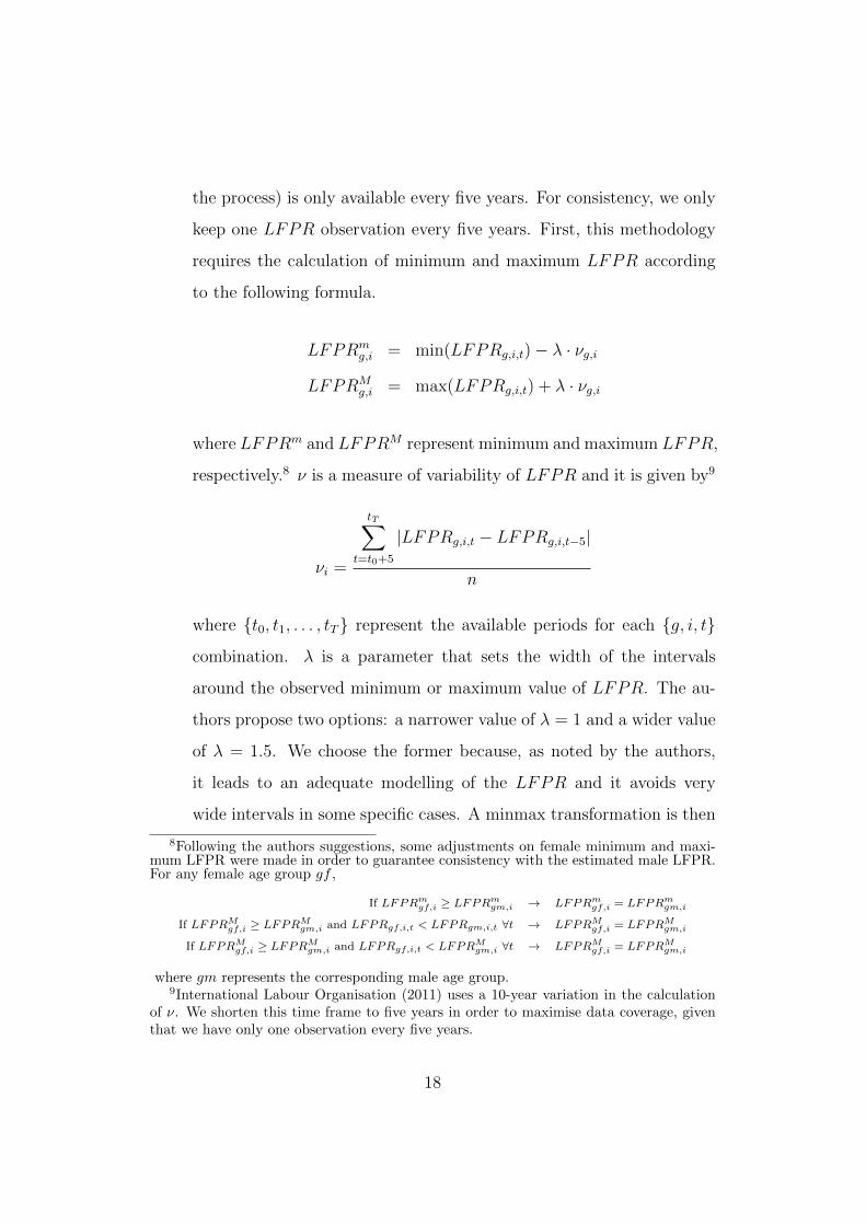
the process) is only available every five years. For consistency, we only

keep one LFPR observation every five years. First, this methodology

requires the calculation of minimum and maximum LFPR according

to the following formula.

LFPRmg,i = min(LFPRg,i,t)− λ · νg,i

LFPRMg,i = max(LFPRg,i,t) + λ · νg,i

where LFPRm and LFPRM represent minimum and maximum LFPR,

respectively.8 ν is a measure of variability of LFPR and it is given by9

νi =

tT∑t=t0+5

|LFPRg,i,t − LFPRg,i,t−5|

n

where {t0, t1, . . . , tT} represent the available periods for each {g, i, t}

combination. λ is a parameter that sets the width of the intervals

around the observed minimum or maximum value of LFPR. The au-

thors propose two options: a narrower value of λ = 1 and a wider value

of λ = 1.5. We choose the former because, as noted by the authors,

it leads to an adequate modelling of the LFPR and it avoids very

wide intervals in some specific cases. A minmax transformation is then

8Following the authors suggestions, some adjustments on female minimum and maxi-mum LFPR were made in order to guarantee consistency with the estimated male LFPR.For any female age group gf ,

If LFPRmgf,i ≥ LFPRmgm,i → LFPRmgf,i = LFPRmgm,i

If LFPRMgf,i ≥ LFPRMgm,i and LFPRgf,i,t < LFPRgm,i,t ∀t → LFPRMgf,i = LFPRMgm,i

If LFPRMgf,i ≥ LFPRMgm,i and LFPRgf,i,t < LFPRMgm,i ∀t → LFPRMgf,i = LFPRMgm,i

where gm represents the corresponding male age group.9International Labour Organisation (2011) uses a 10-year variation in the calculation

of ν. We shorten this time frame to five years in order to maximise data coverage, giventhat we have only one observation every five years.

18

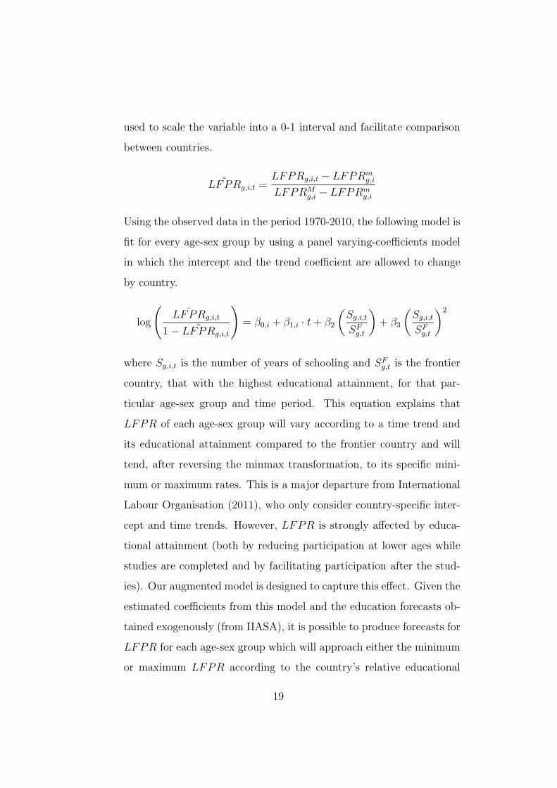
used to scale the variable into a 0-1 interval and facilitate comparison

between countries.

˜LFPRg,i,t =LFPRg,i,t − LFPRm

g,i

LFPRMg,i − LFPRm

g,i

Using the observed data in the period 1970-2010, the following model is

fit for every age-sex group by using a panel varying-coefficients model

in which the intercept and the trend coefficient are allowed to change

by country.

log

(˜LFPRg,i,t

1− ˜LFPRg,i,t

)= β0,i + β1,i · t+ β2

(Sg,i,tSFg,t

)+ β3

(Sg,i,tSFg,t

)2

where Sg,i,t is the number of years of schooling and SFg,t is the frontier

country, that with the highest educational attainment, for that par-

ticular age-sex group and time period. This equation explains that

LFPR of each age-sex group will vary according to a time trend and

its educational attainment compared to the frontier country and will

tend, after reversing the minmax transformation, to its specific mini-

mum or maximum rates. This is a major departure from International

Labour Organisation (2011), who only consider country-specific inter-

cept and time trends. However, LFPR is strongly affected by educa-

tional attainment (both by reducing participation at lower ages while

studies are completed and by facilitating participation after the stud-

ies). Our augmented model is designed to capture this effect. Given the

estimated coefficients from this model and the education forecasts ob-

tained exogenously (from IIASA), it is possible to produce forecasts for

LFPR for each age-sex group which will approach either the minimum

or maximum LFPR according to the country’s relative educational

19

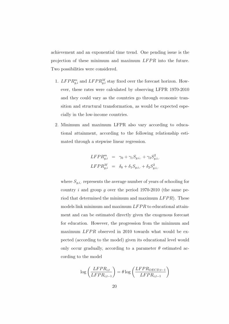
achievement and an exponential time trend. One pending issue is the

projection of these minimum and maximum LFPR into the future.

Two possibilities were considered.

1. LFPRmg,i and LFPRM

g,i stay fixed over the forecast horizon. How-

ever, these rates were calculated by observing LFPR 1970-2010

and they could vary as the countries go through economic tran-

sition and structural transformation, as would be expected espe-

cially in the low-income countries.

2. Minimum and maximum LFPR also vary according to educa-

tional attainment, according to the following relationship esti-

mated through a stepwise linear regression.

LFPRmg,i = γ0 + γ1Sg,i,· + γ2S

2g,i,·

LFPRMg,i = δ0 + δ1Sg,i,· + δ2S

2g,i,·

where Sg,i,· represents the average number of years of schooling for

country i and group g over the period 1970-2010 (the same pe-

riod that determined the minimum and maximum LFPR). These

models link minimum and maximum LFPR to educational attain-

ment and can be estimated directly given the exogenous forecast

for education. However, the progression from the minimum and

maximum LFPR observed in 2010 towards what would be ex-

pected (according to the model) given its educational level would

only occur gradually, according to a parameter θ estimated ac-

cording to the model

log

(LFPRi,t

LFPRi,t−1

)= θ log

(LFPROECD,t−1

LFPRi,t−1

)20

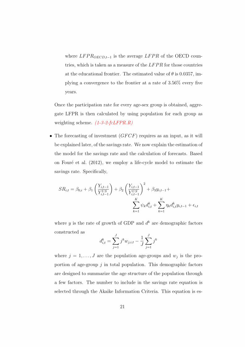
where LFPROECD,t−1 is the average LFPR of the OECD coun-

tries, which is taken as a measure of the LFPR for those countries

at the educational frontier. The estimated value of θ is 0.0357, im-

plying a convergence to the frontier at a rate of 3.56% every five

years.

Once the participation rate for every age-sex group is obtained, aggre-

gate LFPR is then calculated by using population for each group as

weighting scheme. (1-3-2-fcLFPR.R)

• The forecasting of investment (GFCF ) requires as an input, as it will

be explained later, of the savings rate. We now explain the estimation of

the model for the savings rate and the calculation of forecasts. Based

on Foure et al. (2012), we employ a life-cycle model to estimate the

savings rate. Specifically,

SRi,t = β0,i + β1

(Yi,t−1

Y USi,t−1

)+ β2

(Yi,t−1

Y USi,t−1

)2

+ β3yi,t−1+

K∑k=1

ψkdki,t +

K∑k=1

ηkdki,tyi,t−1 + εi,t

where y is the rate of growth of GDP and dk are demographic factors

constructed as

dki,t =J∑j=1

jkwj,i,t −1

J

J∑j=1

jk

where j = 1, . . . , J are the population age-groups and wj is the pro-

portion of age-group j in total population. This demographic factors

are designed to summarize the age structure of the population through

a few factors. The number to include in the savings rate equation is

selected through the Akaike Information Criteria. This equation is es-

21

timated through random-effects. Five-year averages are used in the

estimation in order to correct for the business cycle (why not use trend

savings rate?) Note that, according to this model, the savings rate

depends on lagged values of GDP (in relation to the frontier GDP),

so that it can be calculated recursively with GDP. The savings rate

through the life cycle is given by the following figure (calculated at

the median rate of growth of GDP). The savings rate is then used to

estimate and forecast investment rates. (1-3-3-fcSR.R)

• Instead of imposing an exogenous rate of GFCF and therefore K, as

in Johansson et al. (2012), we follow Foure et al. (2012) and estimate a

Feldstein-Horioka relationship linking domestic savings and investment.

According to this model, investment depends on the rate of savings in

a closed economy. However, as financial openness progresses, financing

for investment can be obtained from the international financial markets

and the relationship between domestic savings and investment becomes

weaker. This is estimated through an error-correction model.

∆

(GCF

Y

)i,t

= α1,i+α2,i

[(GCF

Y

)i,t−1

− β1

(SR

Y

)i,t−1

− β2,iΓ1,i,t−1

β3,iΓ2,i,t−1

]+ α3∆

(SR

Y

)i,t

+ α4,i∆Γ1,i,t + α5,iΓ2,i,t + εi,t

Following Giannone and Lenza (2008), we estimate an factor-augmented

model to take into account the influence of the financial conditions on

investment. To achieve this, we take three series: OECD investment

rate, US long-term interest rate and G7 long-term interest rate. We

calculate a principal components models of the three variables and keep

22

the first two components (they explain 98.6% of the cumulative vari-

ance). This creates a complication when calculating the current invest-

ment rate as it requires the OECD investment rate, which is determined

simultaneously. However, this problem can be overcome by iterating

the estimation until the coefficients stabilize. (1-1-8-SRandIR.R)

3 Way forward

The walkthrough described above covers the first component of the research

project, as described at the beginning of this document. The study will

proceed by incorporating the endogenous effect of conflict in each of the

growth determinants included above. This will then feed into a forecasting

framework that will simulate simultaneously, future conflict-growth paths

for all countries of the world. The results could be important inputs in

determining the likely onsets of conflict and their possible impact on long-

term economic growth and, ultimately, in the lives of the affected population.

For an update of the research activity at a later date, please contact the

author.

References

Backus, D. K. and Kehoe, P. J. (1992). International evidence of the historical

properties of business cycles, American Economic Review 82(4): 864–888.

Balakrishnan, R., Cardarelli, R., Estrada, M., Igan, D., Lusinyan, L., Ma-

hedy, T., Sole, J., Turunen, J., Zook, J., Dao, M. C., Gray, S., King,

D. and Westelius, N. (2014). United States, Selected issues, International

Monetary Fund.

23

Berlemann, M. and Wesselhoft, J.-E. (2014). Estimating aggregate capital

stocks using the perpetual inventory method. a survey of previous im-

plementations and new empirical evidence for 103 countries, Review of

Economics 65(1): 1–34.

Foure, J., Benassy-Quere, A. and Fontagne, L. (2012). The great shift:

macroeconomic projections for the world ecoenomy at the 2050 horizon,

Working Papers 3, CEPII.

Giannone, D. and Lenza, M. (2008). The feldstein-horioka fact, Working

Paper Seriess 873, European Central Bank.

Hegre, H., Karlsen, J., Nygard, H., Strand, H. and Urdal, H. (2013). Predict-

ing armed conflict, 2011–2050, International Studies Quarterly 57(2): 250–

270.

International Labour Organisation (2011). ILO estimates and projections

of the economically active population: 1990-2020 (sixth edition). Method-

ological description, Technical report, International Labour Organisation.

Johansson, A., Guillemette, Y., Murtin, F., Turner, D., Nicoletti, G., de la

Maisonneuve, C., Bagnoli, P., Bousquet, G. and Spinelli, F. (2012). Long-

term growth scenarios, Working Papers 1000, OECD Economics Depar-

ment.

Morrison, C. and Murtin, F. (2010). The Kuznets curve of education: a

global perspective on education inequalities, Working Papers 116, Centre

for the Economics of Education, London School of Economics.

Ravn, M. O. and Uhlig, H. (2002). On adjusting the Hodrick-Prescott filter

for the frequency of observations, The Review of Economics and Statistics

84(2): 371–375.

24

A Compendium of equations

This appendix provides a list of the main structural equations that com-

pose the forecasting macroeconomic model. For definitions of symbols and

25

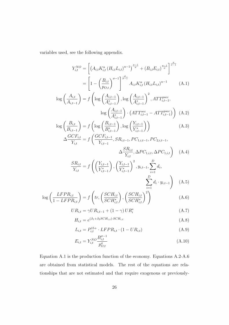
variables used, see the following appendix.

Y NOi,t =

[(Ai,tK

αi,t (Hi,tLi,t)

α−1)σ−1σ + (Bi,tEi,t)

σ−1σ

] σσ−1

=

[1−

(Bi,t

pO,t

)σ−1] σσ−1

Ai,tKαi,t (Hi,tLi,t)

α−1 (A.1)

log

(Ai,tAi,t−1

)= f

(log

(Ai,t−1

A∗i,t−1

), log

(Ai,t−1

A∗i,t−1

)2

, ATT pseci,t−1,

log

(Ai,t−1

A∗i,t−1

)·(ATT seci,t−1 − ATT

pseci,t−1

))(A.2)

log

(Bi,t

Bi,t−1

)= f

(log

(Bi,t−1

B∗i,t−1

), log

(Yi,t−1

Y ∗i,t−1

))(A.3)

∆GCFi,tYi,t

= f

(GCFi,t−1

Yi,t−1

, SRi,t−1, PC1,i,t−1, PC2,i,t−1,

∆SRi,t

Yi,t,∆PC1,i,t,∆PC1,i,t

)(A.4)

SRi,t

Yi,t= f

((Yi,t−1

Y ∗i,t−1

),

(Yi,t−1

Y ∗i,t−1

)2

, yi,t−1,D∑i=1

di,

D∑i=1

di · yi,t−1

)(A.5)

log

(LFPRi,t

1− LFPRi,t

)= f

(tr,

(SCHi,t

SCH∗i,t

),

(SCHi,t

SCH∗i,t

)2)

(A.6)

URi,t = γURi,t−1 + (1− γ)UR∗i (A.7)

Hi,t = e(β1+β2SCHi,t)·SCHi,t (A.8)

Li,t = P 15+i,t · LFPRi,t · (1− URi,t) (A.9)

Ei,t = Y NOi,t

Bσ−1i,t

pσO,t(A.10)

Equation A.1 is the production function of the economy. Equations A.2-A.6

are obtained from statistical models. The rest of the equations are rela-

tionships that are not estimated and that require exogenous or previously-

26

calculated values.

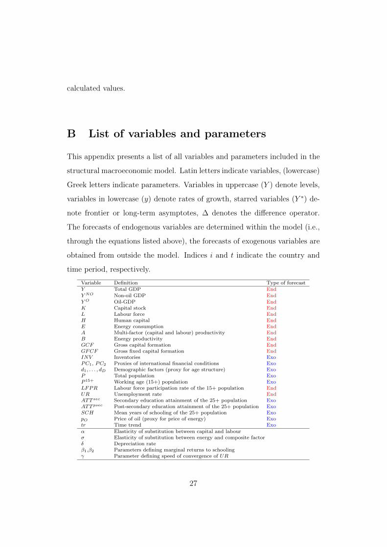
B List of variables and parameters

This appendix presents a list of all variables and parameters included in the

structural macroeconomic model. Latin letters indicate variables, (lowercase)

Greek letters indicate parameters. Variables in uppercase (Y ) denote levels,

variables in lowercase (y) denote rates of growth, starred variables (Y ∗) de-

note frontier or long-term asymptotes, ∆ denotes the difference operator.

The forecasts of endogenous variables are determined within the model (i.e.,

through the equations listed above), the forecasts of exogenous variables are

obtained from outside the model. Indices i and t indicate the country and

time period, respectively.

Variable Definition Type of forecastY Total GDP EndY NO Non-oil GDP EndY O Oil-GDP EndK Capital stock EndL Labour force EndH Human capital EndE Energy consumption EndA Multi-factor (capital and labour) productivity EndB Energy productivity EndGCF Gross capital formation EndGFCF Gross fixed capital formation EndINV Inventories ExoPC1, PC2 Proxies of international financial conditions Exod1, . . . , dD Demographic factors (proxy for age structure) ExoP Total population ExoP 15+ Working age (15+) population ExoLFPR Labour force participation rate of the 15+ population EndUR Unemployment rate EndATT sec Secondary education attainment of the 25+ population ExoATT psec Post-secondary education attainment of the 25+ population ExoSCH Mean years of schooling of the 25+ population ExopO Price of oil (proxy for price of energy) Exotr Time trend Exoα Elasticity of substitution between capital and labourσ Elasticity of substitution between energy and composite factorδ Depreciation rateβ1,β2 Parameters defining marginal returns to schoolingγ Parameter defining speed of convergence of UR

27