Determinants of city growth in Colombia

Gilles Duranton∗‡

University of Pennsylvania

April 2015

Abstract: I develop an integrated approach to examine the drivers ofpopulation growth in Colombian cities between 1993 and 2010. Fertilityplays an important role. Much of the higher growth of some Colombiancities can also be associated with higher wages. In turn, this wageadvantage of some cities can be, in part, traced back to city educationand industry shocks. I also find that roads matter but obtained mixedevidence about the role of urban amenities and no evidence regardingmeasures of urban costs and other drivers of urban growth that havebeen commonly considered by past literature. Some determinants oflong-run city growth are also explored.

Key words: urban growth, Colombia

jel classification: r11, r22

∗I am grateful to Prottoy Akbar for his help with some the data assembled here and Magda Biesiada for her helpwith maps. I am also grateful to Jose Antonio Pinzon, Diana Lopez, Adolfo Meisel, and Fabio Sanchez for providing medata. Finally, thanks to Jan Brueckner and participants to the 2013 neudc conference for very useful remarks

‡Wharton School, University of Pennsylvania, 3620 Locust Walk, Philadelphia, pa 19104, usa (e-mail: duran-

ton@wharton.upenn.edu; website: https://real-estate.wharton.upenn.edu/profile/21470/). Also affiliated withthe Center for Economic Policy Research, the Spatial Economic Centre at the London School of Economics, and theRimini Centre for Economic Analysis.

1. Introduction

This paper examines the drivers of population growth in Colombian cities between 1993 and 2010.

Its main novelty is to consider a comprehensive set of determinants. I uncover a number of

important results. First, fertility plays an important role. Cities with higher growth also enjoy

stronger inflows of newcomers and fewer out-migrants. Then, much of the higher growth of

some Colombian cities can also be associated with higher wages and productivity. In turn, this

productivity advantage can be, in part, traced back to city education and industry shocks. City

education nonetheless affects city growth beyond contemporaneous wages. I also find that city

roads matter both because they facilitate travel within the city and, perhaps to a lesser extent,

because they give better access to other cities. I obtained mixed evidence about the role of urban

amenities and no evidence regarding measures of urban costs or other drivers of urban growth

that have been commonly considered in past literature. Taken together, these findings suggest that

Colombian cities should be considered first as local labour markets.

Taking an integrated approach to the determinants of urban growth is important for several

reasons. First, many countries attempt to control the location of their population and limit the

growth of their cities. Desmet and Henderson (2015) report that 80% of governments in developing

countries are concerned by the geographic distribution of their population and 70% have policies

in place to reduce internal migrations. Example abound in developing countries, from China’s

hukou system to restrictions on mobility and urbanisation in India or Tanzania. Many developed

countries, including France and the uk, also have a strong tradition of centralised policies to

affect urban evolutions. They use instruments such as location-based incentives for firms or the

relocation of public sector activities. Understanding the drivers of urban growth and their strength

is also useful to assess whether restrictive policies can have any effect at all and what their welfare

implications might be. More generally, knowing what drives urban growth is an important first

step to assess how much people gain from moving to a city.

Second, it is the case that growing cities in developing countries require massive investments

to accompany their population growth. According to Glaeser (2011), America’s cities in 1900 were

spending as much on their water system as the federal government spent on everything, except

for the military and its pensions. These investments have then extremely long-lasting implications.

For instance, the streets dug by Roman soldiers more than 2000 years ago when creating new cities

1

in Western Europe are often still major arteries today. Better sanitation in cities in Europe and

North America has had immense and long lasting public health consequences. The beautification

of Paris by Baron Haussmann nearly 150 years ago is still a fundamental reason why so many

tourist visits this city and a major amenity for its population. To be able to invest in a timely

manner in major urban infrastructure such as water, roads, school, or sanitation, it is important

to have the best possible predictions about future urban growth. While the drivers of tomorrow’s

growth may not be the same as those of yesterday’s, a good understanding of what drives urban

growth is likely to yield better results than simple extrapolations. Both under- and over-investment

in infrastructure can be very costly. Investing in the ‘wrong’ cities is also costly.

Considering a large set of possible drivers of urban growth is also of academic importance. With

the main exception of Glaeser, Scheinkman, and Shleifer (1995) who consider a limited number of

factors ranging from human capital to local policies, much of the literature on the growth of cities

has so far focused on making the case for one particular driver or another without really con-

fronting these drivers to each other. For instance, Glaeser, Kallal, Scheinkman, and Shleifer (1992)

focus on a few characteristics of the production structure of cities, Glaeser and Saiz (2004) focus on

human capital, Rappaport (2007) and Carlino and Saiz (2008) focus on amenities, Duranton and

Turner (2012) focus on roads, etc. A lot has been learnt from ‘one-factor’ studies. In particular,

these studies have started recently to pay attention to causal identification by developing a range

of instrumental variable strategies (e.g., Duranton and Turner, 2012). The objective of this paper

is to retain what has been learnt from these one-factor studies, in terms of both substantial results

and methodology, but upgrade their approach to a larger collection of factors. This paper also fills

a number of gaps regarding determinants that have been neglected by recent literature such as the

level of wages, local demography, or local governments.

Finally, this study is also a rare study looking at urban growth in a development context. While

there is now a well-established literature about the growth of cities in developed countries (see

Duranton and Puga, 2014, for a recent review), very little is known about the systematic drivers

of urban growth in developing cities. Work by da Mata, Deichmann, Henderson, Lall, and Wang

(2007), who examine the growth of Brazilian cities, is a rare exception.1 This paucity of literature is

all the more surprising given that the number of cities with more than 100,000 inhabitants nearly

1One may also mention the work by Deliktas, Önder, and Karadag (2013) on Turkish cities but it is of more limitedscope. Duranton (2014a) reviews more broadly the literature on cities and growth in developing countries.

2

trebled between 1960 and 2000 and another two billion urban dwellers are expected over the next

50 years (Henderson and Venables, 2009). While there is little doubt that a staggering number of

people will move to cities, it is deeply unclear which cities they will choose. Looking at a more

advanced developing country like Colombia should be informative in this respect.

The first main challenge to the development of an integrated approach to urban growth is one

of data. Being able to consider most of the key drivers of urban growth requires a broad array of

city level variables. For this purpose, I collected rich municipal data for Colombia. Among others,

they cover city demographics, history, economics (including the composition of economic activity),

geography, amenities, infrastructure, the built environment, public finances, etc. I also rely on data

about trade and agglomeration produced in prior work (Duranton, 2014b, 2015).

The second main challenge regards the identification of the causal effect of city characteristics

on city growth. Standard urban growth regressions typically regress city population growth over

a period of time on a set of city characteristics at the initial period. However, being predetermined

does not make an explanatory variable exogenous. Many decisions are made on the basis of

expectations about future local growth. While climate and many other geographical characteristics

of cities are arguably exogenous, it is hard to make a similar case for most other potential drivers

of city growth.2

In absence of large-scale randomised experimentation about urban growth or natural exper-

iments, instrumental variables are going to provide the main levers used to establish causality.

Plausible instruments are unfortunately not available for each and every possible driver of urban

growth, only for some of them. Based on previous literature, early road networks provide rea-

sonable predictors for current roads networks and, after using appropriate controls for long-run

growth, a good case can be made that these road networks are correlated with contemporaneous

population growth only through current roads. For some other variables such as city education,

one can rely on the number universities and institutions of higher learning. This increases the lag

between the measure of education used in the regression and contemporaneous growth but does

not make the variation used for identification unquestionably exogenous. For some variables, such

as local wages, it is even harder to provide any instrument. Hence, although this paper endeavours

to use best practice from extant research, it is by no means perfect and these limitations will need

2Even though climate is, to a first-order approximation, ‘exogenous’, nothing guarantees that its coefficient is appro-priately identified in standard urban growth regressions. This is because climate is likely to be correlated with otherdeterminants of urban growth which may be missing from these regressions. See below for further discussion.

3

to be kept in mind when interpreting the results.

The rest of this paper is organised as follows. Section 2 describes the data at hand. Section 3

discusses the main drivers of urban growth and the literature on the subject. Section 4 reports the

main results regarding the demographic and productivity determinants of urban growth. Section

5 reports results regarding amenities, roads, and other determinants of urban growth. Section 6

examines the determinants of the long-run growth of cities. Finally, section 7 concludes.

2. Context and data

At the end of our study period in 2010, the population of Colombia was about 44 million over

a territory of 1.1 million square kilometers. It is located at the Northern tip of South America.

Like many countries of the continent, it is already highly urbanised with 75% of its population

living in cities. It is also economically more advanced than developing countries in Africa and

much of Asia with a gdp per capita of about $8,000. Importantly for our purpose Colombia has a

balanced urban system with 60 municipalities with a population above 100,000. This is in contrast

with other developing countries dominated by a primate city. Another attractive feature is that the

boundaries of Colombian municipalities have been extremely stable over time.3 This enables both

the use of deep population lags as controls and the exploration of long-run population growth

patterns.

Note also that the geography of Colombia is extremely varied with much of its territory ei-

ther dominated by the mountains of the Andes or, at the other extreme lowlands covered by an

equatorial jungle. As a result, most of the Colombian population lives either along the Caribbean

coast or on the high plateaus of the interior. Finally, we also keep in mind the existence of large

regional disparities within Colombia. The gdp per capita of the poorest Colombian department is

only about a sixth of that of Bogotá. Hence, despite a high rate of urbanisation, the Colombian

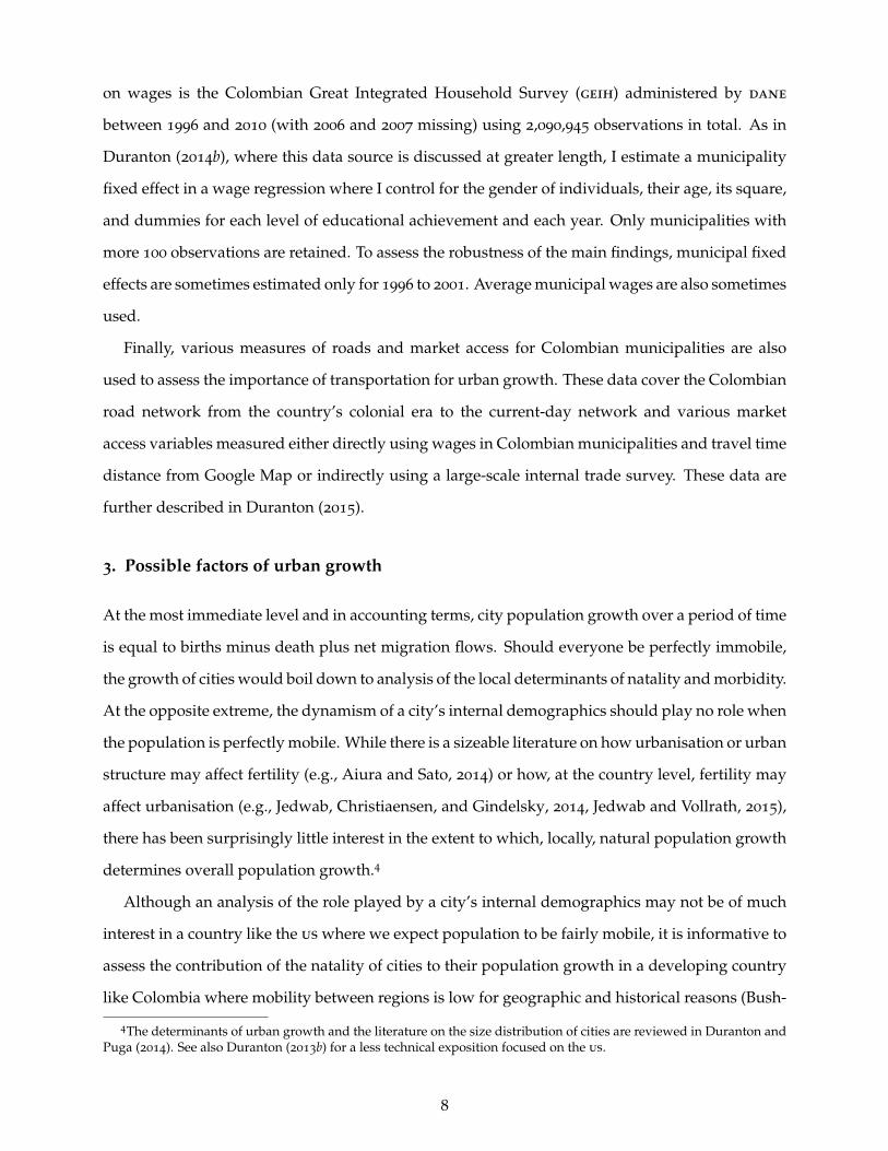
urban system is perhaps far from ‘mature’. See figure 1 for a map and table 1 for some descriptive

statistics about the population of Colombian municipalities.

3The caveat is that this stability is true for the Northwestern half of the country, not for the so-called new departments.Because only a small fraction of the population lives in the Southeastern half of the country, the municipalities in thispart of the country get dropped from our main sample.

4

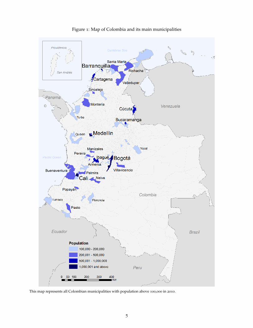
Figure 1: Map of Colombia and its main municipalities

This map represents all Colombian municipalities with population above 100,000 in 2010.

5

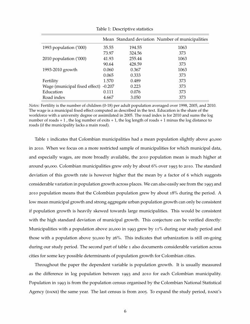
Table 1: Descriptive statistics

Mean Standard deviation Number of municipalities

1993 population (’000) 35.55 194.55 106373.97 324.56 373

2010 population (’000) 41.93 255.44 106390.64 428.59 373

1993-2010 growth 0.060 0.367 10630.065 0.333 373

Fertility 1.570 0.489 373Wage (municipal fixed effect) -0.207 0.223 373Education 0.111 0.076 373Road index 4.667 3.050 373

Notes: Fertility is the number of children (0-18) per adult population averaged over 1998, 2005, and 2010.The wage is a municipal fixed effect computed as described in the text. Education is the share of theworkforce with a university degree or assimilated in 2005. The road index is for 2010 and sums the lognumber of roads + 1 , the log number of exits + 1, the log length of roads + 1 minus the log distance toroads (if the municipality lacks a main road).

Table 1 indicates that Colombian municipalities had a mean population slightly above 40,000

in 2010. When we focus on a more restricted sample of municipalities for which municipal data,

and especially wages, are more broadly available, the 2010 population mean is much higher at

around 90,000. Colombian municipalities grew only by about 6% over 1993 to 2010. The standard

deviation of this growth rate is however higher that the mean by a factor of 6 which suggests

considerable variation in population growth across places. We can also easily see from the 1993 and

2010 population means that the Colombian population grew by about 18% during the period. A

low mean municipal growth and strong aggregate urban population growth can only be consistent

if population growth is heavily skewed towards large municipalities. This would be consistent

with the high standard deviation of municipal growth. This conjecture can be verified directly:

Municipalities with a population above 20,000 in 1993 grew by 11% during our study period and

those with a population above 50,000 by 26%. This indicates that urbanization is still on-going

during our study period. The second part of table 1 also documents considerable variation across

cities for some key possible determinants of population growth for Colombian cities.

Throughout the paper the dependent variable is population growth. It is usually measured

as the difference in log population between 1993 and 2010 for each Colombian municipality.

Population in 1993 is from the population census organised by the Colombian National Statistical

Agency (dane) the same year. The last census is from 2005. To expand the study period, dane’s

6

population estimates for 2010 are used. These population estimates are not mere projections of

the 2005 population data. They take migration flows, births, and deaths between 2005 and 2010

into account. I nonetheless verify the robustness of the main results using population growth from

1993 to 2005.

To control for past growth trends, log census populations from 1918, 1938, 1951, and 1964 are

often included as controls. In some regressions, I also use log population change between 1938

and 2010 as dependent variable and control for population in 1912, 1851, and 1843. Finally, some

regressions even consider population growth since 1870 or 1843. Historical population data for

Colombia are discussed in Duranton (2014b).

While most of the analysis is done at the level of Colombian municipalities, I verify below

that the results are robust to using population in the ‘core’ of the municipality as Colombian

data often distinguish between the (urban) core of a municipality and the (rural) periphery. For

large cities, most of the population lives in the core. More rural areas have a larger share of

population living outside the core. In some regressions, I also verify that the main results are

robust to using metropolitan areas instead of municipalities. Metropolitan areas are defined as in

Duranton (2013a) using cross-municipal commuting patterns. This makes little difference because

only 22 metropolitan areas are formed of more than one municipality. Most of the 99 satellite

municipalities that send more than 10% of their work force to other parts of their metropolitan

areas are suburban municipalities located in the immediate vicinity of the largest Colombian urban

cores. Because most of the analysis below is performed on a sample of municipalities with a large

population, I often refer to them as cities.

To measure many aspects of Colombian municipalities, I use a wealth of data from dane and

provided to me by the National Planning Ministry (dnp). These variables measure demographic

changes, education, housing, and local public finances. Measures of the structure of employment

in Colombian municipalities are computed from the 1990 and 2005 census of production. Sánchez

and Nuñez (2000) gathered a large number of geographical characteristics for Colombian munici-

palities including climate, availability of natural resources such as gold, coal, or oil, altitude, soils,

or availability of water among others. Meisel Roca and Pérez (2012) also collected a rich set of

amenity and tourism variables containing information about museums, public libraries, hotels,

restaurants, and airport arrivals and departures.

Wages play a particularly important role in the analysis below. The main source of information

7

on wages is the Colombian Great Integrated Household Survey (geih) administered by dane

between 1996 and 2010 (with 2006 and 2007 missing) using 2,090,945 observations in total. As in

Duranton (2014b), where this data source is discussed at greater length, I estimate a municipality

fixed effect in a wage regression where I control for the gender of individuals, their age, its square,

and dummies for each level of educational achievement and each year. Only municipalities with

more 100 observations are retained. To assess the robustness of the main findings, municipal fixed

effects are sometimes estimated only for 1996 to 2001. Average municipal wages are also sometimes

used.

Finally, various measures of roads and market access for Colombian municipalities are also

used to assess the importance of transportation for urban growth. These data cover the Colombian

road network from the country’s colonial era to the current-day network and various market

access variables measured either directly using wages in Colombian municipalities and travel time

distance from Google Map or indirectly using a large-scale internal trade survey. These data are

further described in Duranton (2015).

3. Possible factors of urban growth

At the most immediate level and in accounting terms, city population growth over a period of time

is equal to births minus death plus net migration flows. Should everyone be perfectly immobile,

the growth of cities would boil down to analysis of the local determinants of natality and morbidity.

At the opposite extreme, the dynamism of a city’s internal demographics should play no role when

the population is perfectly mobile. While there is a sizeable literature on how urbanisation or urban

structure may affect fertility (e.g., Aiura and Sato, 2014) or how, at the country level, fertility may

affect urbanisation (e.g., Jedwab, Christiaensen, and Gindelsky, 2014, Jedwab and Vollrath, 2015),

there has been surprisingly little interest in the extent to which, locally, natural population growth

determines overall population growth.4

Although an analysis of the role played by a city’s internal demographics may not be of much

interest in a country like the us where we expect population to be fairly mobile, it is informative to

assess the contribution of the natality of cities to their population growth in a developing country

like Colombia where mobility between regions is low for geographic and historical reasons (Bush-

4The determinants of urban growth and the literature on the size distribution of cities are reviewed in Duranton andPuga (2014). See also Duranton (2013b) for a less technical exposition focused on the us.

8

nell, 1993). The difficult geography of the country has led Colombian regions to evolve in relative

isolation from each other. As a result, they have developed different regional cultures and senses

of belonging. Beyond this, the demographic question is salient in Colombia where demographic

differences across cities are extremely large. For instance, the 2010 birth rate in Quibdó, the main

city of the Chocó region along the Pacific coast, is about 50% higher than in Cartagena, the fourth

largest city on the Caribbean coast. The 2010 birth rate in Quibdó is also twice as high as in Bogotá,

the capital and largest city, and three times as high as in Medellín, the second largest city. Relative

to the low-fertility cities of the Coffee region, the natality gap is even higher.

After demography, initial population is another crucial variable that is at the heart of three

important issues regarding urban growth. First, there is a worry that large cities in developing

countries may be growing faster than smaller cities, and, somehow, may be growing too big.

For many years, Colombia was hailed as a virtuous example of a country with a balanced urban

system, which included four major cities in roughly the same size league. This is in contrast with a

country like Argentina for which the metropolitan area around the main city, Buenos Aires, hosts

nearly a third of the country population. Greater Buenos Aires is also nearly 10 times as large as

the second largest metropolitan area. This said, the last decades have seen the rising prominence

of Bogotá in the Colombian urban system. This may be a concern in a country where a balance

between the main regions is perceived as important politically.

Whether the population growth of cities depends on their initial size has also important implica-

tions for the long-run size distribution of cities. In particular, there has been a salient controversy

in the literature regarding whether Gibrat’s law holds for city population growth. Gibrat’s law

(a.k.a., the law of proportional effects) is the statement that growth over a period is orthogonal to

the initial level. In turn, Gibrat’s law implies either a log normal city size distribution or a Pareto

distribution (a.k.a., Zipf’s law) depending on minute differences regarding the growth of cities

at the bottom tail. Both distributions appear to be appropriate first-order description of the size

distribution of cities.5

The third reason why initial population size should be included in city growth regressions is

more technical. Consider first a hypothetical situation where population is highly mobile across

5See Eeckhout (2004) and subsequent literature for the Gibrat’s law controversy for us cities. The relationshipbetween the size distribution of cities and their growth is discussed at length in Duranton and Puga (2014). See Duranton(2013a) for a discussion of the size distribution of Colombian cities. See finally, Ioannides and Skouras (2013) for a recentdiscussion of how to evaluate the shape of the distribution of city sizes.

9

cities. Then, a change in a city’s characteristics leads to a change in its population soon afterwards.

To be concrete, assume that a new road leads to an almost immediate influx of population. To

capture this type of phenomenon, it is appropriate to regress changes in city population on changes

in the roadway using a ‘difference-on-differences’ regression. However, as noted by Duranton and

Turner (2012), if population only gradually adjusts to the new infrastructure, one should regress

changes in population on the initial level of roads and initial population. Given that our results

about city demographics strongly suggest that mobility is far from perfect in Colombia, regressing

city population changes on the initial levels of population and key determinants of population also

measured in level appears appropriate. Estimating this type of ‘difference-on-levels’ regression is

in line with much of the literature on urban growth.6

Then, from standard reasoning, we expect net migration flows in or out of a city to be de-

termined by the wages and incomes that this city offers, the quality of life in this city, and the

costs of living in this city, mainly determined by housing and transportation costs. Regressing

city population growth on city wages constitutes an interesting exercise for two reasons. First,

incomes and wages are arguably important proximate causes of urban growth. Obviously, the

causal effect of city wages on city population is unlikely to be perfectly identified from such

regression. Importantly, the estimated elasticity of wages with respect to population is likely to

be downward-biased since we expect workers to base their location decisions on long-run wages

not on the wages measured for any given year (which are also likely to be mismeasured). Wages

and population growth are also expected to be simultaneously determined as population inflows

will lower local wages (at least in the short run).

Second, it is also interesting to estimate the effect of other, perhaps deeper, factors of urban

growth in conjunction with wages. For instance, human capital in a city may cause urban growth

for a variety of reasons. City human capital may increase productivity through local human capital

externalities. It may also increase future productivity through learning by workers surrounded

by more educated workers. Alternatively, a larger share of more educated workers in a city may

generate local amenities that are directly valued by the residents. Considering wages and measures

of city human capital both together and separately in city growth regressions will be informative

and provide suggestive evidence regarding the channels through which city education affects city

growth.

6See Duranton and Puga (2014) for further discussion of this issue.

10

It is somewhat puzzling that wages and productivity are seldom used in city growth regres-

sions. An early exception is Glaeser et al. (1995), who consider wages in conjunction with other

determinants of population growth for us cities, but estimate mostly insignificant coefficients.

More recently, Beaudry, Green, and Sand (2014) have developed a new approach to estimating

the effects of changes in city wages on city population growth. Their estimation strategy relies on

differences in national wage premia across sectors. More specifically, wages in a city are expected to

grow faster when sectors with high premia become locally more important or if the more important

sectors of activity of a city experience a growing premium nationally. For us cities, Beaudry et al.

(2014) estimate an elasticity of city population with respect to city wages of about two over a

ten-year time horizon.

As already stated, high wages can only constitute a proximate factor of city population growth

just like aggregate investment is a proximate factor of gdp growth. To go deeper, it is important

to understand what drives urban wages. It seems natural to expect higher wages to result from a

stronger demand for labour locally. The demand for labour may increase for idiosyncratic reasons

following, for instance, the breakthrough of an entrepreneur who develops a very successful

new business.7 There may also be a systematic component to changes in labour demand. As

sectors of economic activity rise and decline at the national level, cities with a ‘favourable’ mix

of sectors should experience rising wages and increasing population while cities with an adverse

mix will decline. Following Bartik (1991), it has become commonplace to use city shares of sectoral

employment multiplied by their national growth and summed across sectors as a more exogenous

surrogate for city employment growth. Although these predictors of city growth have often been

used as instruments for population growth, when the latter is used as an explanatory variable for

something else, there has been very little work that focuses on the effects of changes in labour

demand on city population.

In Duranton (2014b), I examine determinants of local wages to estimate agglomeration effects

in Colombian cities. While its focus is different, this analysis of agglomeration effects leads a

to number of findings that are relevant here. Most importantly, there is some evidence, albeit

modest, that city education, as measured by the share of university graduates, and market access

7In Duranton (2007), I explore the implications of such idiosyncratic discoveries for the size distribution of cities inan urban system. I also provide empirical evidence about some of these implications including the fast churning ofsectoral employment in cities. Following Glaeser et al. (1992), there have been many claims regarding the importanceof entrepreneurship in local growth. These issues are best explored by focusing on the evolution of employment at thelevel of sectors of economic activity across locations. This will constitute the object of a separate analysis.

11

both matter in determining wages. On the other hand, there is no evidence that roads or amenities

have any effect on wages.

Following Glaeser et al. (1995), Simon and Nardinelli (2002), Glaeser and Saiz (2004), and many

others, city-wide measures of human capital have often been considered in city growth regressions.

While human capital in an area can be measured in many ways, the share of university-educated

workers is a popular measure. For 20th- and 21st-century cities in developed countries, this

measure of city-wide human capital is usually a strong and robust predictor of future growth.

The evidence for earlier periods is also supportive, though not as strongly. Simon and Nardinelli

(1996) find robust evidence of an important role of human capital for the growth of English cities

in the second part of the 19th century and the first part of the 20th. For us counties over the last 200

years, Glaeser, Ponzetto, and Tobio (2014) find an uneven role for city human capital in the early

part of their study period.

After Moretti (2004) and others, a strong case can be made that a greater proportion of university

graduates in a city in the us is associated with higher wages. Although, as already mentioned, the

evidence for this type of effect is less strong in Colombia, this is certainly a possible channel of

transmission. Because city education may generate human capital externalities that translate into

higher wages, more education in a city will eventually lead to an inflow of newcomers.

While a direct effect of city education on wages is possibly a key channel of transmission, this

need not be the only one. There may be more to the relationship between city education and wages

as higher wages may also be a delayed response to human capital externalities that generate some

learning. In the extreme, workers might migrate to a city in large numbers to learn and then leave

to reap the benefits from their learning elsewhere. As a result, much of the effect of city human

capital may not go through contemporaneous wages and we may observe an important effect of

city human capital on subsequent growth even after controlling for city wages. Following, Shapiro

(2006), it is also possible that human capital affects city growth through the formation of positive

local amenities associated with human capital.

Regressing city population growth on the initial level of city human capital may not identify

a causal effect of city human capital on population growth. More educated workers might be

flocking to growing cities ahead of other workers, perhaps because they are more mobile. More

prosperous cities, which grow faster, may also be able to provide their residents with more and

better education. The literature on us cities has used the establishment of land grant colleges in

12

the second part of the 19th century in small places at the centre of many states as a source of

exogenous variation for city education (Moretti, 2004, Shapiro, 2006). The estimates that use this

source of variation confirm those of simple cross-sectional regressions. Glaeser and Saiz (2004)

perform a number of other robustness checks and further buttress the case that city education has

causal effect on city population growth in us cities.

Urban amenities are also often acknowledged to play an important role in the growth of cities.

While standard economic analysis in the spirit of Roback (1982) makes it clear that cities with better

amenities should be larger, it is less immediately obvious that cities with better amenities should

grow faster. A key reason behind the possible positive effect of amenities on city growth could be

that urban amenities are normal goods (or even perhaps luxury goods) for which households are

willing to pay increasingly high prices as they get richer.

There is strong empirical evidence regarding the role of a specific amenity in us urban growth:

the weather. Glaeser, Kolko, and Saiz (2001) argue that January and July temperatures are the

most reliable predictors of city growth in recent us history. These findings have been confirmed

by subsequent literature in the us and by Cheshire and Magrini (2006) for European countries. It

could nonetheless be the case that good weather is correlated with another potential explanation

of city population growth. For instance, warm January temperatures in the us are predominantly

found in the South. Southern us cities also make it easier to build housing, a potential confounding

factor. Fears of a spurious correlation have been alleviated by Rappaport (2007) who shows that

the relationship between good weather and population growth is true outside of the us South.

Adding to this, Carlino and Saiz (2008) show that tourism visits, which may be understood as

an overall measure of amenities, is a robust predictor of city population growth in the us even

after controlling for weather. They also provide plausible instruments which confirm their main

results. Taken together, findings by extant literature strongly support the notion of a positive effect

of amenities, and particularly of nice weather, on city growth. Whether such findings also hold in

developing cities is an open question.

The transportation infrastructure, the road infrastructure in particular, is another possible de-

terminant of urban growth that has been considered in the literature. Urban roads may matter

for two reasons. First, they are expected to ease travel within cities and allow residents to reach

their destinations, work in particular at a lower costs. In turn, roads will induce them to travel

further to reach better jobs or restaurants they like better. Roads will also allow residents to travel

13

more often. Lower travel costs will also alleviate the scarcity of land and thus lower housing costs.

Standard economic models of city structure in the spirit of Alonso (1964), Mills (1967), and Muth

(1969) imply that more roads should make cities more attractive and thus foster their population

growth. Duranton and Turner (2012) provide some evidence regarding the role of roads in the

growth of us cities between 1984 and 2004. They claim that a 10% increase in a city’s roadway

leads to a 1.5% larger population 20 years later. These results have been replicated for various

countries, including Spain (García-López, Holl, and Viladecans-Marsal, 2014).

The second reason why urban roads matter is that they offer convenient ways in and out of

the cities and foster trade. Duranton, Morrow, and Turner (2014) provide evidence that us cities

with more interstate highways export more in volume because of this. In Duranton (2015), I show

that a similar effects also occur in Colombian cities for both exports and imports, in volume and

in value. The main difficulty when regressing urban outcomes on city roads is that roads may

follow from these ‘outcomes’ rather than cause them or that city population growth and roads are

simultaneously determined.

Several solutions to this identification issue have been proposed (see Redding and Turner, 2015,

for a review). Duranton and Turner (2012) use old road networks as exogenous predictors for

current urban roads. These include a plan of the us interstate highway system prior to its devel-

opment after 1956, late 19th century railroads, and early exploration routes of the continent. These

instruments are statistically powerful enough predictors of the current transportation network

since initial highway maps have been by and large implemented, old railroads have often been

turned into roads, and old exploration routes have been slowly upgraded into modern roads. A

case can also be made in favour of their exogeneity since old road networks were mostly about

linking cities whereas our concern here is mostly about travel within cities. This case can be made

stronger by controlling for possible factors that may be correlated with both contemporaneous city

population growth and old road networks such as geographic features or the long run propensity

of some cities to grow. We follow a similar approach here and use data extracted from maps of old

road networks from Colombia dating back to the colonial era.

Beyond roads, the relative location of cities may also matter. Cities with good market access

may grow more. For instance, Redding and Sturm (2008) document that (West) German cities

close to the Iron Curtain, which divided Germany for nearly 30 years, lost much of their market

access after the Iron Curtain was erected. They also experienced a process of relative population

14

decline. Being close to large markets has nonetheless theoretically ambiguous implications. A city

with large markets nearby will enjoy a higher demand for its products. It will also face stiffer

competition from producers located in these neighbouring markets. The resulting effect of these

two forces will be in general non-linear and will depend on subtle issues such as the nature of

competition on product markets (Head and Mayer, 2004).

As imentioned above, there are strong reasons to expect city wages to affect city population

growth. By the same line of reasoning, a higher cost of living could potentially affect negatively city

population growth. While developing a good measure of the overall cost of living in Colombian

cities is beyond the scope of this paper, I can nonetheless use some measures of housing costs to

provide a preliminary exploration of this issue. Finally, the popular press (especially in Colombia)

is always keen to highlight the role of local leadership in cities. Even though I am not able to

establish causality, I can nonetheless provide an early exploration of correlations between some

unique measures of local governance and city population growth.

4. Key drivers of the growth of Colombian cities

All the regressions estimated below are of the same general form:

∆t,t+1 log popc = α log popct + Xctβ + εct , (1)

where the dependent variable is the change in log population between t and t + 1. I usually take

1993 as the beginning of the study period and 2010 as its end. Cities are indexed by c and X is a

vector of city characteristics. These characteristics include a number of variables of interest such

as city wages, education, or roads, among others. They also include a number of control variables

such as regional or departmental dummies and past log populations.

An important issue to note here is that most of the regressions below regress a difference in

population on the initial level of the determinants of urban growth. As already discussed, this is

justified when equilibrium population adjusts only slowly to changes. The first part of the analysis

that follows makes the case that population mobility is far from perfect in Colombia by focusing

on city demographics.

A full accounting exercise that decomposes changes in the population of all cities into births,

deaths, and migration flows in and out of the city is beyond the scope of this paper for two

reasons. The first is that counts of births are available only for certain years and information about

15

migration flows is even more restricted. Birth rates are computed using the number of birth per

adult population in 1993, 2005, and 2010. Migrations flows are only available since 2008 and it

is unclear how precisely the Colombian government is able to track households that move.8 The

second reason for not doing a full accounting exercise is that using a regression like described in

equation (1) will make it easier to compare the results about city demographics with those for other

determinants of city growth.

In table 2, column 1 regresses the change in log population between 1993 and 2010 on log 1993

population and the log birth rate for all available Colombian municipalities. The coefficient on log

initial city population is insignificant. This is a precisely estimated zero since the standard error

on this elasticity is less than 0.01. The coefficient on log birth rate is 0.24 and highly significant.

Again, under perfect mobility, this coefficient is expected to be zero as natality in a city should be

uncorrelated with its population growth rate.9 Under perfect immobility, this coefficient should be

close to one as the population can only increase through births.10

Column 2 of table 2 uses a broader measure of internal demographic dynamism. Namely, it

replaces the birth rate used in column 1 by a fertility rate computed using the number of children

below the age of 18 relative to the adult population. This alternative measure yields a marginally

higher coefficient of 0.27 instead of 0.24, perhaps because it measures long-run fertility better.

Column 3 uses instead the log counts of migrants in and out of the city. The coefficient on out

migrants is negative and low at -0.04. The coefficient on in-migrants is much larger and positive

at 0.11. Considering flows of migrants together with the fertility rate in column 4 makes little

difference to the results obtained so far. In essence, growing cities are cities with stronger internal

demographic dynamism, greater flows of in-migrants, and smaller flows of out-migrants. While

the analysis does not allow us to cleanly compare the contributions of fertility and migration

flows to urban growth, we can note that the sum of the coefficients on migration flows is slightly

smaller than the coefficient on fertility but of the same magnitude. It is also easy to see that both

migration flows and fertility appear to have roughly the same explanatory power with respect to

urban population growth. This suggests that both migration and fertility are equally important

8Unfortunately, this variable is only available towards the end of the study period. This may not matter much as weexpect this type of variable to be persistent over time.

9This also requires a lack of correlation between natality and other determinants of city population growth notconsidered in the regression. This issue is tackled below.

10In absence of mobility, city growth should be entirely explained by the differential between natality and mortality.

16

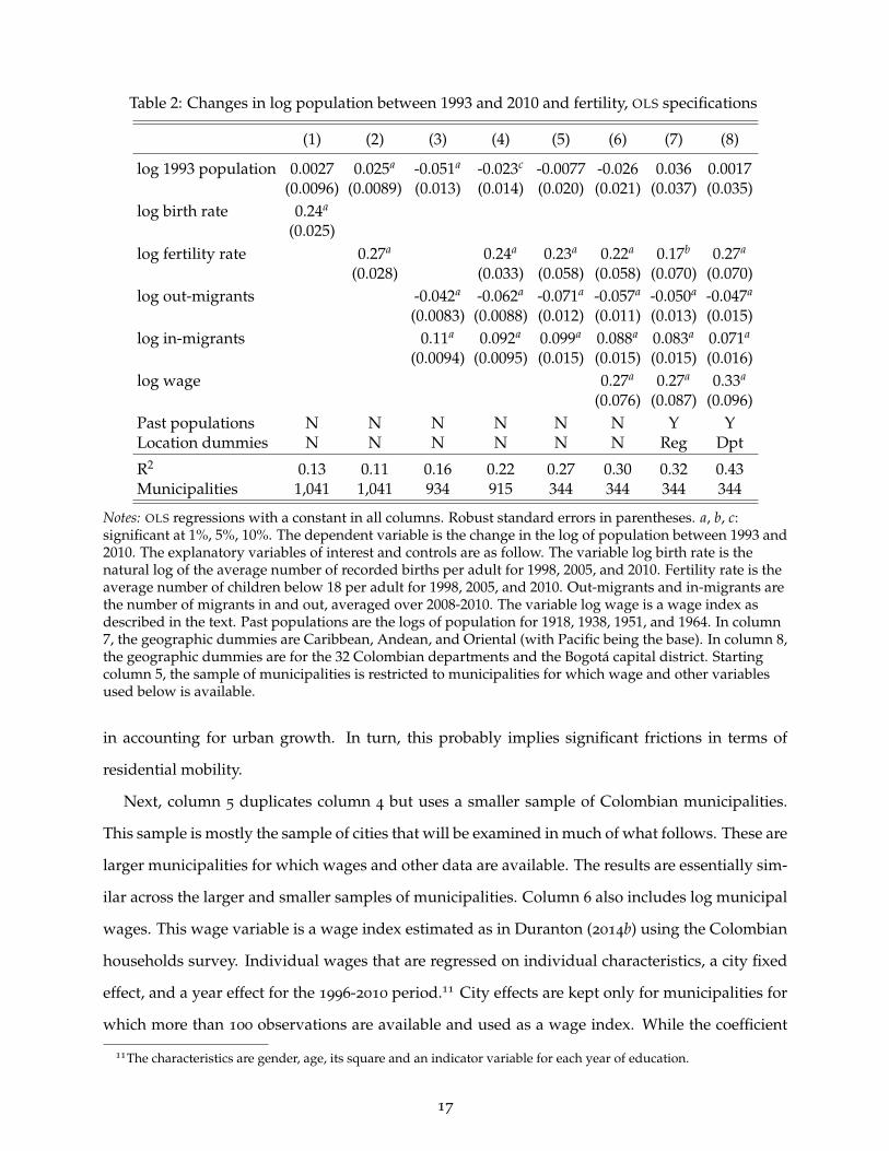
Table 2: Changes in log population between 1993 and 2010 and fertility, OLS specifications

(1) (2) (3) (4) (5) (6) (7) (8)

log 1993 population 0.0027 0.025a -0.051a -0.023c -0.0077 -0.026 0.036 0.0017(0.0096) (0.0089) (0.013) (0.014) (0.020) (0.021) (0.037) (0.035)

log birth rate 0.24a

(0.025)log fertility rate 0.27a 0.24a 0.23a 0.22a 0.17b 0.27a

(0.028) (0.033) (0.058) (0.058) (0.070) (0.070)log out-migrants -0.042a -0.062a -0.071a -0.057a -0.050a -0.047a

(0.0083) (0.0088) (0.012) (0.011) (0.013) (0.015)log in-migrants 0.11a 0.092a 0.099a 0.088a 0.083a 0.071a

(0.0094) (0.0095) (0.015) (0.015) (0.015) (0.016)log wage 0.27a 0.27a 0.33a

(0.076) (0.087) (0.096)Past populations N N N N N N Y YLocation dummies N N N N N N Reg Dpt

R2 0.13 0.11 0.16 0.22 0.27 0.30 0.32 0.43Municipalities 1,041 1,041 934 915 344 344 344 344

Notes: OLS regressions with a constant in all columns. Robust standard errors in parentheses. a, b, c:significant at 1%, 5%, 10%. The dependent variable is the change in the log of population between 1993 and2010. The explanatory variables of interest and controls are as follow. The variable log birth rate is thenatural log of the average number of recorded births per adult for 1998, 2005, and 2010. Fertility rate is theaverage number of children below 18 per adult for 1998, 2005, and 2010. Out-migrants and in-migrants arethe number of migrants in and out, averaged over 2008-2010. The variable log wage is a wage index asdescribed in the text. Past populations are the logs of population for 1918, 1938, 1951, and 1964. In column7, the geographic dummies are Caribbean, Andean, and Oriental (with Pacific being the base). In column 8,the geographic dummies are for the 32 Colombian departments and the Bogotá capital district. Startingcolumn 5, the sample of municipalities is restricted to municipalities for which wage and other variablesused below is available.

in accounting for urban growth. In turn, this probably implies significant frictions in terms of

residential mobility.

Next, column 5 duplicates column 4 but uses a smaller sample of Colombian municipalities.

This sample is mostly the sample of cities that will be examined in much of what follows. These are

larger municipalities for which wages and other data are available. The results are essentially sim-

ilar across the larger and smaller samples of municipalities. Column 6 also includes log municipal

wages. This wage variable is a wage index estimated as in Duranton (2014b) using the Colombian

households survey. Individual wages that are regressed on individual characteristics, a city fixed

effect, and a year effect for the 1996-2010 period.11 City effects are kept only for municipalities for

which more than 100 observations are available and used as a wage index. While the coefficient

11The characteristics are gender, age, its square and an indicator variable for each year of education.

17

on log wages is fairly large at 0.27 and highly significant, the coefficient on natality remains the

same while those on migration are only marginally lower in size. Column 7 further adds indicator

variables for the four main regions of Colombia and log population in 1918, 1938, 1951, and 1964 as

control variables. These controls are important for two reasons. First, regression (1) is equivalent

to regressing the log of 2010 population on the same variable for 1993. If the error term is serially

auto-correlated, this can bias the estimation of the coefficient on initial population. Hopefully the

bias, if any, will be much attenuated by adding further population lags as controls. We also expect

past populations over nearly a century to control for many important unobservables that drive

city growth and could be correlated with city demographics. Column 8 restricts identification

further by also imposing indicator variables for departments. Despite only considering variation

within fairly small units, the coefficients on the demographic variables remain about the same as

in column 6.

The first important lesson that can be drawn from table 2 is that migrations in and out of

cities play in important role as proximate factor for the population growth of cities in Colombia.

Although this probably was to be expected, this legitimises the rest of this analysis and an attempt

to understand what makes some cities more attractive to newcomers. The second main lesson from

table 2 is that city fertility plays, perhaps, a surprisingly large role. Cities with a higher fertility

grow faster with an elasticity of about 0.25. Hence, while there is some mobility, it is far from

perfect and this justifies our focus in most of what follows on differences-on-levels regressions

instead of differences-on-differences regressions. Since city demographics is only a proximate

factor behind city growth, for the rest of the analysis we turn to deeper determinants and ignore

city demographics.

A third finding of table 2 is the suggestion that wages also play an important role in city growth.

The regressions reported in table 3 provide further support for this result. Column 1 regresses the

change in log population between 1993 and 2010 on log wages. The estimated elasticity is 0.50.

Adding initial population, past populations and regional indicators in column 2 or departmental

indicators in column 3 makes little difference. Again, these wages by city are estimated from

the Colombian labour force survey over the period and finely control for standard observable

characteristics of workers such as their gender, age, and educational achievement. To assess the

effect of this particular choice, column 4 uses mean wages computed directly from the data. This

18

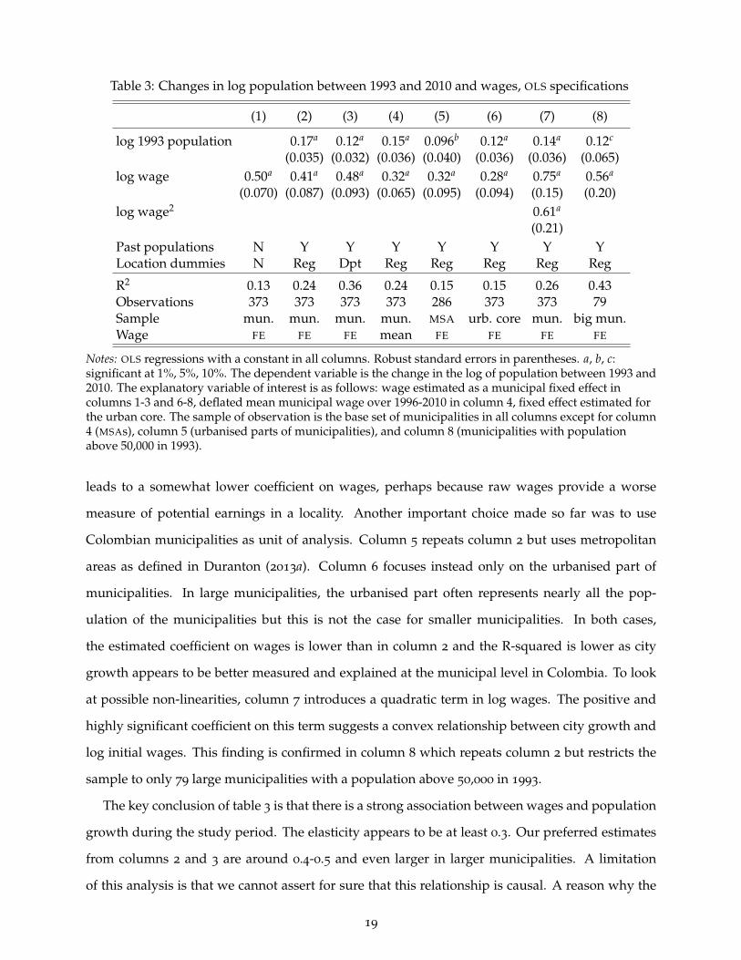
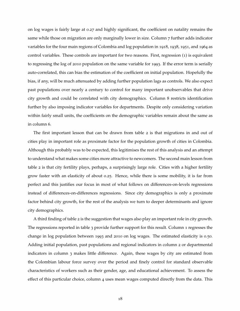
Table 3: Changes in log population between 1993 and 2010 and wages, OLS specifications

(1) (2) (3) (4) (5) (6) (7) (8)

log 1993 population 0.17a 0.12a 0.15a 0.096b 0.12a 0.14a 0.12c

(0.035) (0.032) (0.036) (0.040) (0.036) (0.036) (0.065)log wage 0.50a 0.41a 0.48a 0.32a 0.32a 0.28a 0.75a 0.56a

(0.070) (0.087) (0.093) (0.065) (0.095) (0.094) (0.15) (0.20)log wage2 0.61a

(0.21)Past populations N Y Y Y Y Y Y YLocation dummies N Reg Dpt Reg Reg Reg Reg Reg

R2 0.13 0.24 0.36 0.24 0.15 0.15 0.26 0.43Observations 373 373 373 373 286 373 373 79Sample mun. mun. mun. mun. MSA urb. core mun. big mun.Wage FE FE FE mean FE FE FE FE

Notes: OLS regressions with a constant in all columns. Robust standard errors in parentheses. a, b, c:significant at 1%, 5%, 10%. The dependent variable is the change in the log of population between 1993 and2010. The explanatory variable of interest is as follows: wage estimated as a municipal fixed effect incolumns 1-3 and 6-8, deflated mean municipal wage over 1996-2010 in column 4, fixed effect estimated forthe urban core. The sample of observation is the base set of municipalities in all columns except for column4 (MSAs), column 5 (urbanised parts of municipalities), and column 8 (municipalities with populationabove 50,000 in 1993).

leads to a somewhat lower coefficient on wages, perhaps because raw wages provide a worse

measure of potential earnings in a locality. Another important choice made so far was to use

Colombian municipalities as unit of analysis. Column 5 repeats column 2 but uses metropolitan

areas as defined in Duranton (2013a). Column 6 focuses instead only on the urbanised part of

municipalities. In large municipalities, the urbanised part often represents nearly all the pop-

ulation of the municipalities but this is not the case for smaller municipalities. In both cases,

the estimated coefficient on wages is lower than in column 2 and the R-squared is lower as city

growth appears to be better measured and explained at the municipal level in Colombia. To look

at possible non-linearities, column 7 introduces a quadratic term in log wages. The positive and

highly significant coefficient on this term suggests a convex relationship between city growth and

log initial wages. This finding is confirmed in column 8 which repeats column 2 but restricts the

sample to only 79 large municipalities with a population above 50,000 in 1993.

The key conclusion of table 3 is that there is a strong association between wages and population

growth during the study period. The elasticity appears to be at least 0.3. Our preferred estimates

from columns 2 and 3 are around 0.4-0.5 and even larger in larger municipalities. A limitation

of this analysis is that we cannot assert for sure that this relationship is causal. A reason why the

19

coefficients on wages may be over-estimated is that a greater population may foster wages through

agglomeration effects. In Duranton (2014b), I estimate these ‘opposite’ elasticities to be about an

order of magnitude smaller in Colombian cities. It is hard to be believe that agglomeration effects

could be a major source of bias here. Instead, the coefficients estimated here may be too small as, in

the short run, the arrival of more workers may act to dampen the pressure on wages.12 We return

to the identification of wage effects on urban growth below.

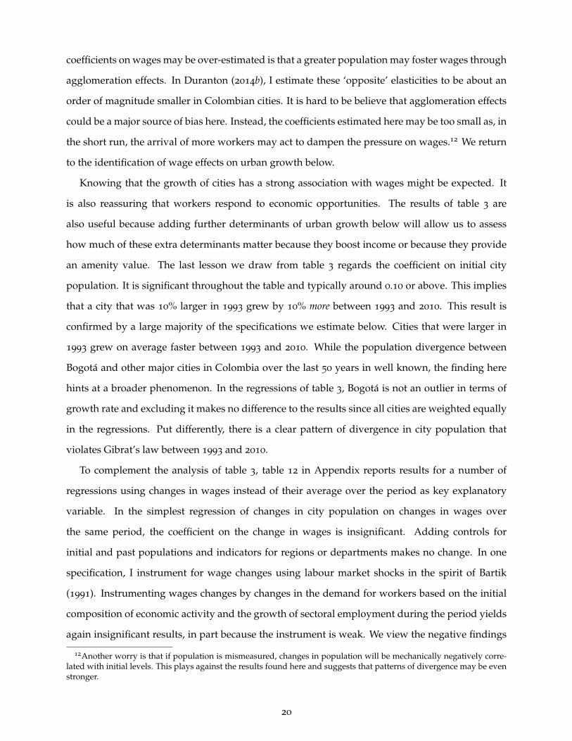
Knowing that the growth of cities has a strong association with wages might be expected. It

is also reassuring that workers respond to economic opportunities. The results of table 3 are

also useful because adding further determinants of urban growth below will allow us to assess

how much of these extra determinants matter because they boost income or because they provide

an amenity value. The last lesson we draw from table 3 regards the coefficient on initial city

population. It is significant throughout the table and typically around 0.10 or above. This implies

that a city that was 10% larger in 1993 grew by 10% more between 1993 and 2010. This result is

confirmed by a large majority of the specifications we estimate below. Cities that were larger in

1993 grew on average faster between 1993 and 2010. While the population divergence between

Bogotá and other major cities in Colombia over the last 50 years in well known, the finding here

hints at a broader phenomenon. In the regressions of table 3, Bogotá is not an outlier in terms of

growth rate and excluding it makes no difference to the results since all cities are weighted equally

in the regressions. Put differently, there is a clear pattern of divergence in city population that

violates Gibrat’s law between 1993 and 2010.

To complement the analysis of table 3, table 12 in Appendix reports results for a number of

regressions using changes in wages instead of their average over the period as key explanatory

variable. In the simplest regression of changes in city population on changes in wages over

the same period, the coefficient on the change in wages is insignificant. Adding controls for

initial and past populations and indicators for regions or departments makes no change. In one

specification, I instrument for wage changes using labour market shocks in the spirit of Bartik

(1991). Instrumenting wages changes by changes in the demand for workers based on the initial

composition of economic activity and the growth of sectoral employment during the period yields

again insignificant results, in part because the instrument is weak. We view the negative findings

12Another worry is that if population is mismeasured, changes in population will be mechanically negatively corre-lated with initial levels. This plays against the results found here and suggests that patterns of divergence may be evenstronger.

20

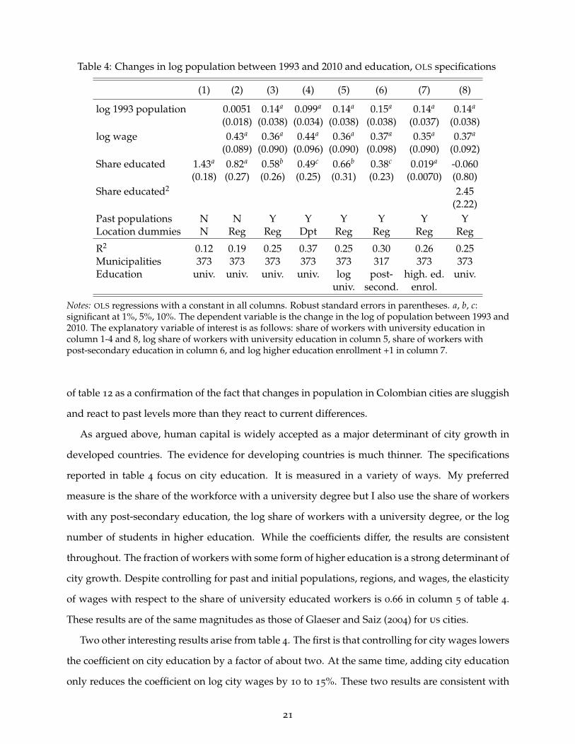
Table 4: Changes in log population between 1993 and 2010 and education, OLS specifications

(1) (2) (3) (4) (5) (6) (7) (8)

log 1993 population 0.0051 0.14a 0.099a 0.14a 0.15a 0.14a 0.14a

(0.018) (0.038) (0.034) (0.038) (0.038) (0.037) (0.038)log wage 0.43a 0.36a 0.44a 0.36a 0.37a 0.35a 0.37a

(0.089) (0.090) (0.096) (0.090) (0.098) (0.090) (0.092)Share educated 1.43a 0.82a 0.58b 0.49c 0.66b 0.38c 0.019a -0.060

(0.18) (0.27) (0.26) (0.25) (0.31) (0.23) (0.0070) (0.80)Share educated2 2.45

(2.22)Past populations N N Y Y Y Y Y YLocation dummies N Reg Reg Dpt Reg Reg Reg Reg

R2 0.12 0.19 0.25 0.37 0.25 0.30 0.26 0.25Municipalities 373 373 373 373 373 317 373 373Education univ. univ. univ. univ. log post- high. ed. univ.

univ. second. enrol.

Notes: OLS regressions with a constant in all columns. Robust standard errors in parentheses. a, b, c:significant at 1%, 5%, 10%. The dependent variable is the change in the log of population between 1993 and2010. The explanatory variable of interest is as follows: share of workers with university education incolumn 1-4 and 8, log share of workers with university education in column 5, share of workers withpost-secondary education in column 6, and log higher education enrollment +1 in column 7.

of table 12 as a confirmation of the fact that changes in population in Colombian cities are sluggish

and react to past levels more than they react to current differences.

As argued above, human capital is widely accepted as a major determinant of city growth in

developed countries. The evidence for developing countries is much thinner. The specifications

reported in table 4 focus on city education. It is measured in a variety of ways. My preferred

measure is the share of the workforce with a university degree but I also use the share of workers

with any post-secondary education, the log share of workers with a university degree, or the log

number of students in higher education. While the coefficients differ, the results are consistent

throughout. The fraction of workers with some form of higher education is a strong determinant of

city growth. Despite controlling for past and initial populations, regions, and wages, the elasticity

of wages with respect to the share of university educated workers is 0.66 in column 5 of table 4.

These results are of the same magnitudes as those of Glaeser and Saiz (2004) for us cities.

Two other interesting results arise from table 4. The first is that controlling for city wages lowers

the coefficient on city education by a factor of about two. At the same time, adding city education

only reduces the coefficient on log city wages by 10 to 15%. These two results are consistent with

21

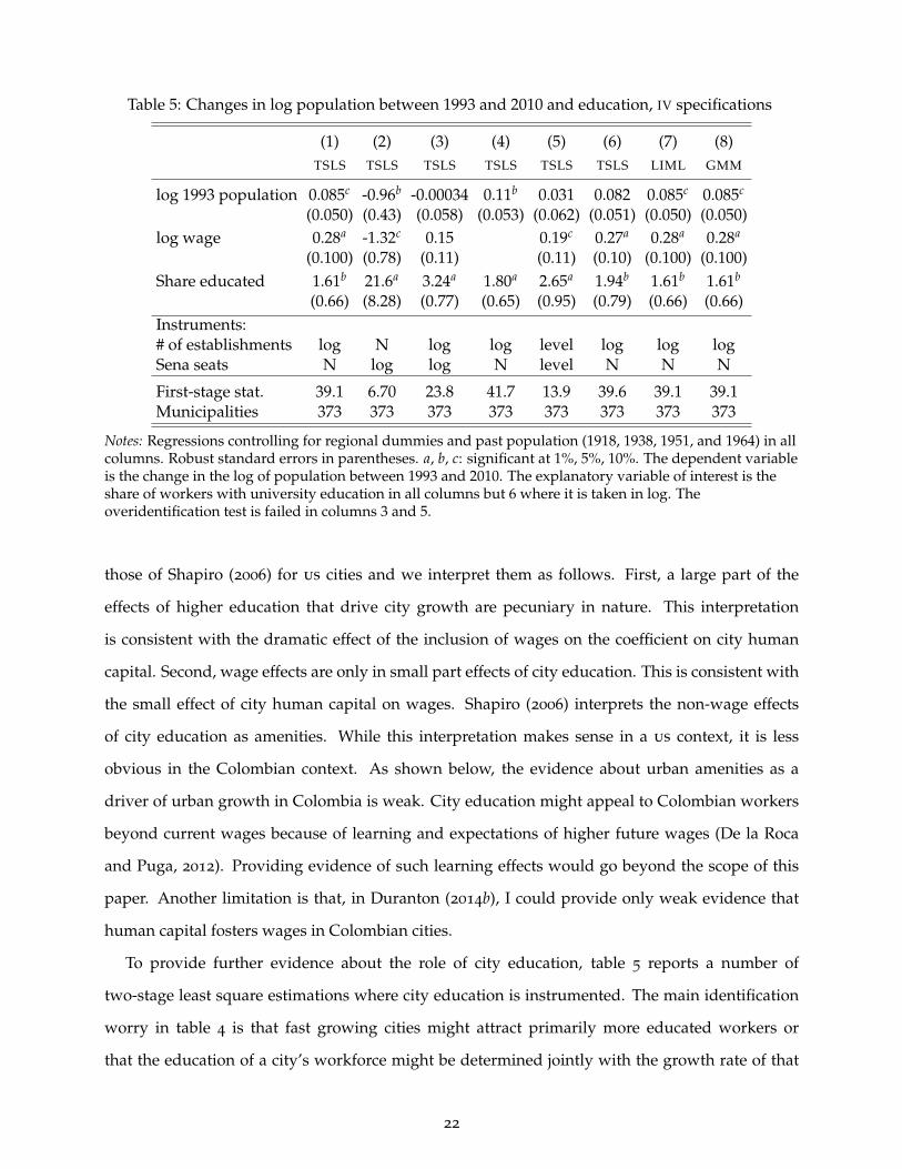
Table 5: Changes in log population between 1993 and 2010 and education, IV specifications

(1) (2) (3) (4) (5) (6) (7) (8)TSLS TSLS TSLS TSLS TSLS TSLS LIML GMM

log 1993 population 0.085c -0.96b -0.00034 0.11b 0.031 0.082 0.085c 0.085c

(0.050) (0.43) (0.058) (0.053) (0.062) (0.051) (0.050) (0.050)log wage 0.28a -1.32c 0.15 0.19c 0.27a 0.28a 0.28a

(0.100) (0.78) (0.11) (0.11) (0.10) (0.100) (0.100)Share educated 1.61b 21.6a 3.24a 1.80a 2.65a 1.94b 1.61b 1.61b

(0.66) (8.28) (0.77) (0.65) (0.95) (0.79) (0.66) (0.66)Instruments:# of establishments log N log log level log log logSena seats N log log N level N N N

First-stage stat. 39.1 6.70 23.8 41.7 13.9 39.6 39.1 39.1Municipalities 373 373 373 373 373 373 373 373

Notes: Regressions controlling for regional dummies and past population (1918, 1938, 1951, and 1964) in allcolumns. Robust standard errors in parentheses. a, b, c: significant at 1%, 5%, 10%. The dependent variableis the change in the log of population between 1993 and 2010. The explanatory variable of interest is theshare of workers with university education in all columns but 6 where it is taken in log. Theoveridentification test is failed in columns 3 and 5.

those of Shapiro (2006) for us cities and we interpret them as follows. First, a large part of the

effects of higher education that drive city growth are pecuniary in nature. This interpretation

is consistent with the dramatic effect of the inclusion of wages on the coefficient on city human

capital. Second, wage effects are only in small part effects of city education. This is consistent with

the small effect of city human capital on wages. Shapiro (2006) interprets the non-wage effects

of city education as amenities. While this interpretation makes sense in a us context, it is less

obvious in the Colombian context. As shown below, the evidence about urban amenities as a

driver of urban growth in Colombia is weak. City education might appeal to Colombian workers

beyond current wages because of learning and expectations of higher future wages (De la Roca

and Puga, 2012). Providing evidence of such learning effects would go beyond the scope of this

paper. Another limitation is that, in Duranton (2014b), I could provide only weak evidence that

human capital fosters wages in Colombian cities.

To provide further evidence about the role of city education, table 5 reports a number of

two-stage least square estimations where city education is instrumented. The main identification

worry in table 4 is that fast growing cities might attract primarily more educated workers or

that the education of a city’s workforce might be determined jointly with the growth rate of that

22

workforce. To address this concern, we need surrogate variables that determine city education

but are not otherwise correlated with city population growth. Put slightly differently, a good

instrument for city education in this context affects the supply of education of a city but not its

demand for education. A possible candidate instrument for city education could be the number

of local university graduates that enter the workforce. A greater rate of new graduate entry in

the workforce is expected to affect the education of a city’s workforce but will be less likely to

be caused by contemporaneous growth especially if we control for past growth through past log

populations. Instead of the number of recent local graduates, I prefer to use the number of higher

education institutions, most of which were established well before our study period.

I also use the number sena seats. The sena (‘SErvicio Nacional de Aprendizaje’ or National

Service of Learning) is a technical teaching institution established in the 1950s throughout the

country. It depends on the Colombian Ministry of Labour and aims to provide a free technical

education to Colombians who cannot afford any other form of learning from the age of 16, while

aiming to improve the technical capabilities of the workforce. Importantly, the sena branches are

present only in some cities and specialised by field of study.13 These locations and specialisations

appear to be stable over time. The number of seats that each branch offers is roughly proportional

to the population of the region it covers in the specialities that it offers. Although the establishment

of the sena is more recent than that of land-grant colleges in the us used by Moretti (2004) and

Shapiro (2006), this instrument is in the same spirit. Even with controls for broad geographic

regions and for past populations, one may think of a number of reasons why the exclusion restric-

tion associated with these two instruments may not not be satisfied. Using the number of higher

education institutions and the number of sena seats nonetheless provides a useful check on the

ols results proposed in table 4.

It is easy to see that, in table 5, the point estimates on instrumented city education are larger

than in ols. Unfortunately and despite the strength of the instruments, the standards errors are

also large so that it is not possible to make a definitive comparison with the ols results above. To

close on the role of city education, we can also note that the share of university educated workers

is retained as an explanatory variable in most of the specifications below. This variable remains

generally significant with a coefficient around one despite considering a broad variety of controls.

13For instance, the branch in Pasto, close to the Pacific Ocean offers training in “logistics, human resources, cook-ing, agriculture, finance, accounting, food preparation, natural resources management, construction, systems, crafts,accounting, livestock management, and pharmaceutical services.”

23

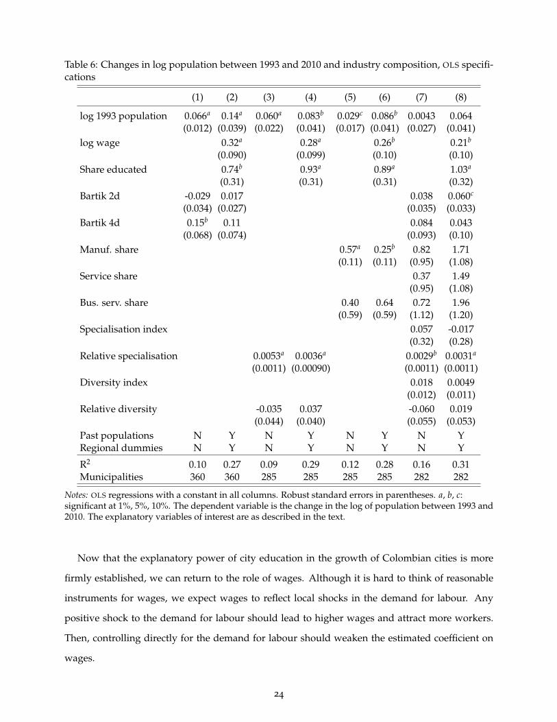
Table 6: Changes in log population between 1993 and 2010 and industry composition, OLS specifi-cations

(1) (2) (3) (4) (5) (6) (7) (8)

log 1993 population 0.066a 0.14a 0.060a 0.083b 0.029c 0.086b 0.0043 0.064(0.012) (0.039) (0.022) (0.041) (0.017) (0.041) (0.027) (0.041)

log wage 0.32a 0.28a 0.26b 0.21b

(0.090) (0.099) (0.10) (0.10)Share educated 0.74b 0.93a 0.89a 1.03a

(0.31) (0.31) (0.31) (0.32)Bartik 2d -0.029 0.017 0.038 0.060c

(0.034) (0.027) (0.035) (0.033)Bartik 4d 0.15b 0.11 0.084 0.043

(0.068) (0.074) (0.093) (0.10)Manuf. share 0.57a 0.25b 0.82 1.71

(0.11) (0.11) (0.95) (1.08)Service share 0.37 1.49

(0.95) (1.08)Bus. serv. share 0.40 0.64 0.72 1.96

(0.59) (0.59) (1.12) (1.20)Specialisation index 0.057 -0.017

(0.32) (0.28)Relative specialisation 0.0053a 0.0036a 0.0029b 0.0031a

(0.0011) (0.00090) (0.0011) (0.0011)Diversity index 0.018 0.0049

(0.012) (0.011)Relative diversity -0.035 0.037 -0.060 0.019

(0.044) (0.040) (0.055) (0.053)Past populations N Y N Y N Y N YRegional dummies N Y N Y N Y N Y

R2 0.10 0.27 0.09 0.29 0.12 0.28 0.16 0.31Municipalities 360 360 285 285 285 285 282 282

Notes: OLS regressions with a constant in all columns. Robust standard errors in parentheses. a, b, c:significant at 1%, 5%, 10%. The dependent variable is the change in the log of population between 1993 and2010. The explanatory variables of interest are as described in the text.

Now that the explanatory power of city education in the growth of Colombian cities is more

firmly established, we can return to the role of wages. Although it is hard to think of reasonable

instruments for wages, we expect wages to reflect local shocks in the demand for labour. Any

positive shock to the demand for labour should lead to higher wages and attract more workers.

Then, controlling directly for the demand for labour should weaken the estimated coefficient on

wages.

24

To measure local shocks to the demand for labour, table 6 uses a variety of metrics. The first

two are standard shifts-share predictors of employment growth in the spirit of Bartik (1991).

These predictors of city employment growth are based on their initial sectoral composition of

employment interacted with the national growth of sectors. I compute them for both two-digit

and four-digit industries. I also cruder measures of the initial composition of employment by

considering the share of employment in manufacturing, business services, and personal services.

Finally, I use finer measures of the composition of economic activity with two specialisation and

two diversity indices. I measure specialisation through the share of the largest four-digit industry

either in absolute terms or relative to its national share in employment. Similarly, I measure

diversity through a Herfindahl index, again of absolute or relative employment as in Duranton

and Puga (2000). Following Glaeser et al. (1992), there is an important body of evidence showing

that patterns of specialisation and diversity provide good predictors of local growth.

A number of conclusions can be drawn from the results of table 6. First, the coefficient on the

wage is divided on average by a factor of around two relative to the specifications in tables 3. That

is, introducing variables that proxy for local labour demand shocks or variables that have been

shown to be associated with local labour changes by past literature has a dramatic effect on the

estimated elasticity of population with respect to wages. Rather than revealing some fragility in

our previous results, we interpret this finding as lending credence to the fundamental importance

of local labour market conditions to explain the growth of cities. Local labour demand shocks will

leads both the number of workers and wages to adjust. That controlling for ‘quantities’ as well as

‘prices’ should lower the estimated coefficient on ‘prices’ is to be expected.

The second main conclusion to be drawn from table 6 is that the coefficient on city human

capital is barely affected by the inclusion of proxies for labour market shocks. We concluded from

tables 4 and 5 that some form of human capital effects were behind part of the wage coefficients we

initially estimated in table 3. From table 6, we just concluded that changes in local labour demand

are an even bigger part of the wage effects. However, controlling for the local composition of

economic activity or for proxies for local labour demand shocks does not appear to affect our

results for city education, as if they were two distinct phenomena. Third, as deeper determinants

of city growth, changes in local labour demand are a big part of the wage effects we initially

estimated. Nonetheless, the variables we introduce in table 6 do not drive the wage coefficient

to zero. Wages appear to affect city growth beyond what happens through city human capital and

25

the local composition of economic activity. As we shall see below, the wage coefficients remain

significant even when we consider further determinants of urban growth.

This said, it would nonetheless be wrong to interpret what is left of the wage effect after

controlling for ‘everything else’ as a ‘pure’ wage effect. The reason is that there might be some

determinants of city growth omitted from this analysis that affect city growth through higher

wages. In addition, the variables we use in table 6 most likely account for changes in local labour

demand only partially.

The last conclusion we can draw from table 6 is less positive and points to the difficulty of

characterising local labour demand changes. Nine different variables are used and only the relative

specialisation index is a consistently significant determinant of city growth. The other measures of

the local composition of economic activity are less robust. They affect the coefficient on wages but

it is hard to pin down one specific metrics that plays a decisive role.

Ultimately, we expect residents to choose their city of residence based on the real wage it offers,

not on its nominal wage. Hence, a lower cost of living could, in theory, act just like a higher wage.

To look at this conjecture in greater detail, the regressions reported in table 13 in appendix consider

a variety of measures or proxies for urban costs. These regressions include the share of land that

is developed, the floor to area ratio in 2005 and 2012, and the average assessed price of residential

space per square metre. All these variables are considered in level or in log depending on the

specification. Unfortunately, the coefficients on these urban costs variables are either insignificant

or, in the case of housing values, have a ‘perverse’ sign. The main problem in these regressions is

that housing values are highly correlated with population and wages as both theory and intuition

suggest they should be. As a result, it is not possible to identify the effects of wages on urban

growth separately from those of property prices. Adding to this, we also expect high property

prices to be a consequence of fast population growth as a well as possible factor that limits it.

Developing a new approach that would allow us to separately identify the (positive) effects of

wages from the (negative) effects of urban costs would go beyond our scope here. We can only

hope future work will tackle this issue.

So far, the results paint a fairly clear picture about urban growth in Colombia. Colombian

cities are labour markets. Places that offer higher wages grow more. We can trace these higher

wages back to local labour shocks and, to a lesser extent, to a more educated workforce. This said,

mobility across these labour markets is far from perfect as evidenced by the fact that the growth

26

of cities is strongly correlated with their internal demographic dynamism. We can also note that,

although wages matter a lot for urban growth, the measured elasticities of population growth with

respect to wages are well below those that have been estimated for the us.

5. Further determinants of urban growth in Colombia

We now turn to further determinants of city growth. As mentioned above, there is a large literature

that highlights the importance of amenities in the growth of us and European cities. This literature

has considered climate and other geographic characteristics of cities. These measures have the

great merit of being more exogenous. More endogenous amenities such as museums, which make

cities nicer, or low crime rates, which make cities more liveable, have also been considered despite

considerable difficulties in identifying causal relationships when such variables are considered.14

The literature has also considered broad summary measures of amenities such as leisure visits

Carlino and Saiz (2008).

The results are reported in table 7. They are generally mixed. In part, these mixed results are

due to data limitations. Some amenity variables are available only for a subset of less than 100

cities. A limited number of observations may be a key reason why the variables associated with

tourism, hospitality (measured through hotels and restaurants), libraries or museums do not yield

any significant result. The evidence about geographic variables is also limited. Precipitations has

a negative significant sign in regressions that include our main sample of more than 300 cities. A

measure of temperature that is available for less than 100 cities has a coefficient that is negative and

significant. This provides modest evidence that a cooler and drier climate may foster city growth.

I did not find robust evidence of a non-linear effect of climate where warm cities located between

1000 and 2000 meters are more attractive than hot coastal cities or colder cities higher up in the

mountains.

The evidence is about violence in what is historically a highly violent country is also limited.

I used various measures of political violence since the 1990s, counting attacks from the various

armed groups or the number of casualties. These measures are arguably of high quality since they

were used internally by the government to guide its counterinsurgency effort. It is also well known

that civil unrest in Colombia led to extremely large population displacements. Despite this, it is

14See Duranton and Puga (2014) for further discussion of this literature.

27

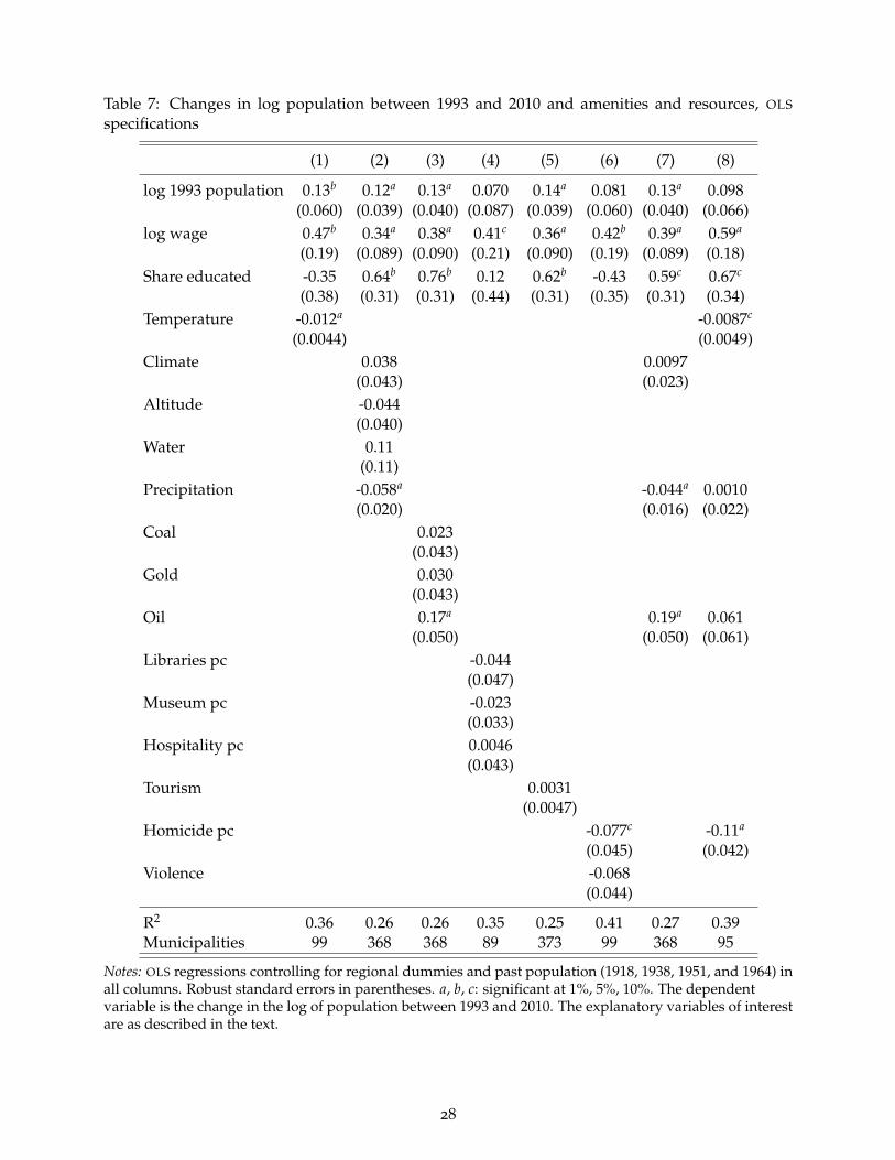
Table 7: Changes in log population between 1993 and 2010 and amenities and resources, OLS

specifications

(1) (2) (3) (4) (5) (6) (7) (8)

log 1993 population 0.13b 0.12a 0.13a 0.070 0.14a 0.081 0.13a 0.098(0.060) (0.039) (0.040) (0.087) (0.039) (0.060) (0.040) (0.066)

log wage 0.47b 0.34a 0.38a 0.41c 0.36a 0.42b 0.39a 0.59a

(0.19) (0.089) (0.090) (0.21) (0.090) (0.19) (0.089) (0.18)Share educated -0.35 0.64b 0.76b 0.12 0.62b -0.43 0.59c 0.67c

(0.38) (0.31) (0.31) (0.44) (0.31) (0.35) (0.31) (0.34)Temperature -0.012a -0.0087c

(0.0044) (0.0049)Climate 0.038 0.0097

(0.043) (0.023)Altitude -0.044

(0.040)Water 0.11

(0.11)Precipitation -0.058a -0.044a 0.0010

(0.020) (0.016) (0.022)Coal 0.023

(0.043)Gold 0.030

(0.043)Oil 0.17a 0.19a 0.061

(0.050) (0.050) (0.061)Libraries pc -0.044

(0.047)Museum pc -0.023

(0.033)Hospitality pc 0.0046

(0.043)Tourism 0.0031

(0.0047)Homicide pc -0.077c -0.11a

(0.045) (0.042)Violence -0.068

(0.044)

R2 0.36 0.26 0.26 0.35 0.25 0.41 0.27 0.39Municipalities 99 368 368 89 373 99 368 95

Notes: OLS regressions controlling for regional dummies and past population (1918, 1938, 1951, and 1964) inall columns. Robust standard errors in parentheses. a, b, c: significant at 1%, 5%, 10%. The dependentvariable is the change in the log of population between 1993 and 2010. The explanatory variables of interestare as described in the text.

28

hard to find much robust and systematic evidence that less exposure to civil unrest is a major driver

of city growth in Colombia. Two speculative reasons can be offered for this, perhaps, surprising

result. First, the end of our study period is in 2010, at least 5 years after political violence became

much less prevalent in Colombia. Second, the worst forms of civil unrest typically took place in

remote rural areas which are not part of the the data used here. In addition, while civil unrest may

have had a large effect on the urbanisation process, it may have been only a push factor for small

municipalities outside our sample, not a pull factor. Displaced rural populations moved to cities

but these populations may not have chosen their city of destination because of their level of civil

unrest, which was much less than in rural areas in most cases. Instead, displaced populations may

have chose more prosperous local labour markets.

While political violence does not appear to explain why some cities grew more than others, city

criminality is negatively associated with cities growth. While data about homicide per capita is

limited to a smaller sample of less than 100 cities, cities with fewer homicides have grown more

between 1993 and 2010. The measured elasticity of city population with respect to homicides per

capita is about -0.1. Nonetheless, this large effect should be interpreted with caution because a

high level of criminality may be determined jointly with other determinants of city growth like a

high level of underemployment. Population growth may also affect criminality.

Finally, table 7 also report results about a number of natural resources. In regressions not

reported here, I also explored the effects of a number of other resources such as precious stones.

The only natural resources that appears to matter is oil. It is robustly significant in most speci-

fications, except when I restrict the sample to the 100 or so large cities for which other measures

of amenities are available. This is arguably because oil in Colombia is overwhelmingly located in

smaller peripheral cities.15

Overall, the evidence regarding amenities is fairly weak. These findings are consistent with

those of Meisel Roca and Pérez (2012). These authors also report that Colombian households spend

a minimal fraction of their income on ‘entertainment’, around 1% instead of 5 to 10% in more

developed countries. Colombian households appear to favour socialising with family members

instead. Regardless of whether these patterns are caused by different cultural preferences or by

the lower level of income in Colombia, it may not be surprising that Colombians are not willing to

move to cities offering better amenities. If they do not spend much for their leisure, they may not

15The ‘oil capital of Colombia’, Barrancabermeja, is an exception with a population above 300,000.

29

want to pay indirectly for amenities by relocating to amenity-rich cities.

Related to amenities, table 14 reports results on a number of other local characteristics which

might affect how appealing a municipality might be. I first used two variables for local inequalities

that measure the unequal distribution of land. None of these two measures is remotely significant.

Then, I also used a measure of stated quality of life. It is highly significant and is associated

positively with population growth. That places for which residents state they enjoy a high quality

of life are also places that retain their existing population and attract newcomers is unsurprising.

This does not say much beyond providing some minimal validation for this stated-preference

variable. Interestingly, this measure of stated quality of life makes the coefficient on city education

insignificant but it barely affects that on wages. This suggests that the stated local quality of life

may not have much to do with wages. In this respect, this finding is mildly puzzling because table

7 struggles to offer robust evidence about local amenities beyond, perhaps, crime and climate.

Finally the last part of the table explores a range of measures of the quality of local government.

These measures were developed for the later part of our study period by the Colombian Planning

Ministry to gather some information about the governance of Colombian municipalities, which,

after the decentralisation reforms of the early 1990s, started to enjoy significant powers without

much oversight by the central government. As argued by Duranton and Puga (2014), very little is

known about the effects of local governance and local leadership on local outcomes such as popu-

lation growth. Nonetheless, these factors are usually strongly emphasised in popular discussions

of local growth and local economic performance.

I use five different measures of local government. The first three are outcome measures. They

concern fiscal performance, a measure of administrative performance, and a measure of overall

performance. I estimate a positive and significant coefficient for these three measures. The last two

measures result from assessments of the administrative capacity of a municipality and the quality

of its management processes. For these two process-based measures, I estimate insignificant

coefficients. While these findings are clearly speculative, the positive and significant associations

between growth and municipal performance together with the absence of a relationship with

the local processes is suggestive of some simultaneity or reverse causation between measures of

municipal performance and growth. Whether the lack of association with measures of processes

is caused by the poor quality of these variables or indicative of something deeper should be the

object of future research.

30

As argued above, there is a strong theoretical case that roads should be a major driver of the

population growth of cities. There is supportive empirical evidence from a variety of countries,

including the us (Duranton and Turner, 2012). Measuring the roadway is challenging in the

present context. While the mileage of highways and major roads is often the explanatory variable

of choice in more developed countries, using it is problematic in an environment where nearly

half the municipalities in 1995 do not have direct access to a major road and where a difficult

geography might distort the mileage. Instead, as in Duranton (2015), I use an index of roads that

accounts for the mileage, the number of road segments (or rays), the number of exits in and out of

a municipality, and the distance to the nearest road for municipalities that do not have any.

Another issue is that for the early part of the study period, my only source of data is a 1995 road

map from the Colombian geographical institute (Instituto Geographicó Agustin Codazzi) which

is fairly sparse. More specifically, this map contains only ‘principal’ roads for which the mileage

is limited.16 For 2012, I use an official map of Colombian roads which contains all roads that

essentially can be used by a truck (principal roads, secondary roads, and ‘carriage’ roads).

Table 8 reports results for a number of ols specifications where the change in log municipal

population between 1993 and 2010 is regressed on a road index for 1995 or for 2012. In line

with previous tables, the more complete specifications control for log wages, the share of higher

education, initial and past populations, and region indicators. This type of specification is close

to those estimated in Duranton and Turner (2012). The estimated coefficient on roads, which can

be loosely interpreted as an elasticity, is small but positive and significant in five specifications in

eight. The three cases where this coefficient is insignificant are precisely estimated zeroes. Looking

at the entire table, we can rule out positive elasticities of 5% or negative elasticities of 3%.

As noted by Duranton and Turner (2012) and many others, the provision of roads is likely to

be simultaneously determined with other local characteristics, many of which are unobserved. To

deal with this identification issue, I follow the same approach as Duranton and Turner (2012) and

instrument contemporaneous roads with long lags of the road network. I also use the same strategy

in Duranton (2015) when I examine the effects of roads on trade between Colombian cities. The

instruments I use are from the 1938 road network and from the colonial road network (‘caminos

16There are about 8,000 kilometers of principal roads reported for 1995. Although, they are called ‘principal’, therewere barely any highways and expressways. A majority of these roads were single lane roads. They are probablybetter described as non-local roads. For the sake of comparison, France, which is about as big as the ‘populated’ part ofColombia, counts more than 400,000 kilometers of non-local roads.

31

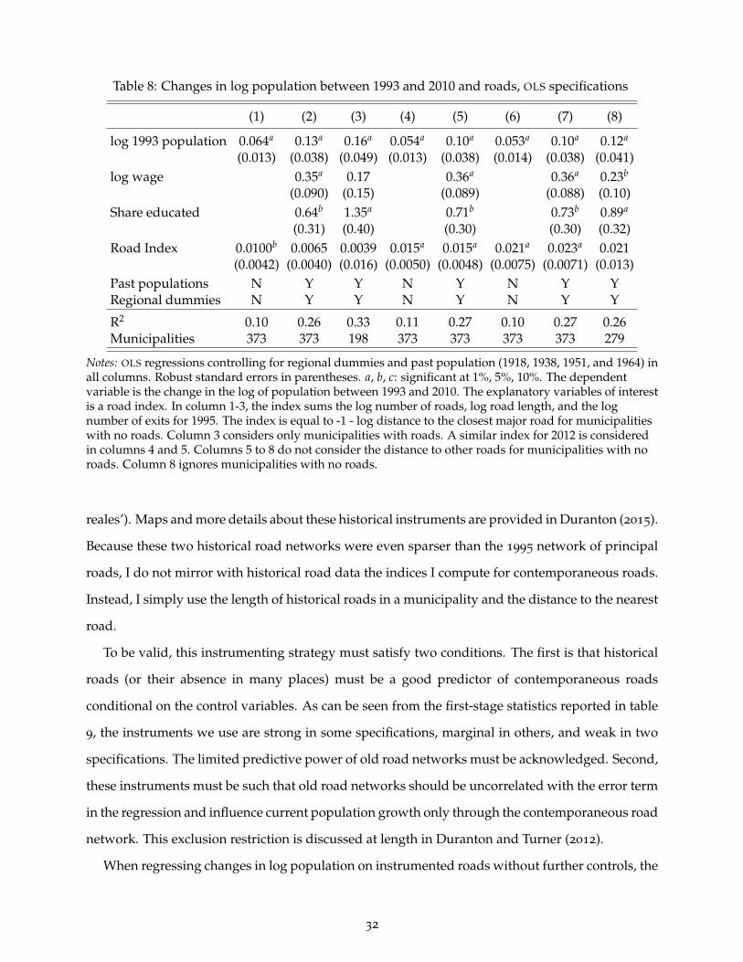
Table 8: Changes in log population between 1993 and 2010 and roads, OLS specifications

(1) (2) (3) (4) (5) (6) (7) (8)

log 1993 population 0.064a 0.13a 0.16a 0.054a 0.10a 0.053a 0.10a 0.12a

(0.013) (0.038) (0.049) (0.013) (0.038) (0.014) (0.038) (0.041)log wage 0.35a 0.17 0.36a 0.36a 0.23b

(0.090) (0.15) (0.089) (0.088) (0.10)Share educated 0.64b 1.35a 0.71b 0.73b 0.89a

(0.31) (0.40) (0.30) (0.30) (0.32)Road Index 0.0100b 0.0065 0.0039 0.015a 0.015a 0.021a 0.023a 0.021

(0.0042) (0.0040) (0.016) (0.0050) (0.0048) (0.0075) (0.0071) (0.013)Past populations N Y Y N Y N Y YRegional dummies N Y Y N Y N Y Y

R2 0.10 0.26 0.33 0.11 0.27 0.10 0.27 0.26Municipalities 373 373 198 373 373 373 373 279

Notes: OLS regressions controlling for regional dummies and past population (1918, 1938, 1951, and 1964) inall columns. Robust standard errors in parentheses. a, b, c: significant at 1%, 5%, 10%. The dependentvariable is the change in the log of population between 1993 and 2010. The explanatory variables of interestis a road index. In column 1-3, the index sums the log number of roads, log road length, and the lognumber of exits for 1995. The index is equal to -1 - log distance to the closest major road for municipalitieswith no roads. Column 3 considers only municipalities with roads. A similar index for 2012 is consideredin columns 4 and 5. Columns 5 to 8 do not consider the distance to other roads for municipalities with noroads. Column 8 ignores municipalities with no roads.

reales’). Maps and more details about these historical instruments are provided in Duranton (2015).

Because these two historical road networks were even sparser than the 1995 network of principal

roads, I do not mirror with historical road data the indices I compute for contemporaneous roads.

Instead, I simply use the length of historical roads in a municipality and the distance to the nearest

road.

To be valid, this instrumenting strategy must satisfy two conditions. The first is that historical

roads (or their absence in many places) must be a good predictor of contemporaneous roads

conditional on the control variables. As can be seen from the first-stage statistics reported in table

9, the instruments we use are strong in some specifications, marginal in others, and weak in two

specifications. The limited predictive power of old road networks must be acknowledged. Second,

these instruments must be such that old road networks should be uncorrelated with the error term

in the regression and influence current population growth only through the contemporaneous road

network. This exclusion restriction is discussed at length in Duranton and Turner (2012).

When regressing changes in log population on instrumented roads without further controls, the

32

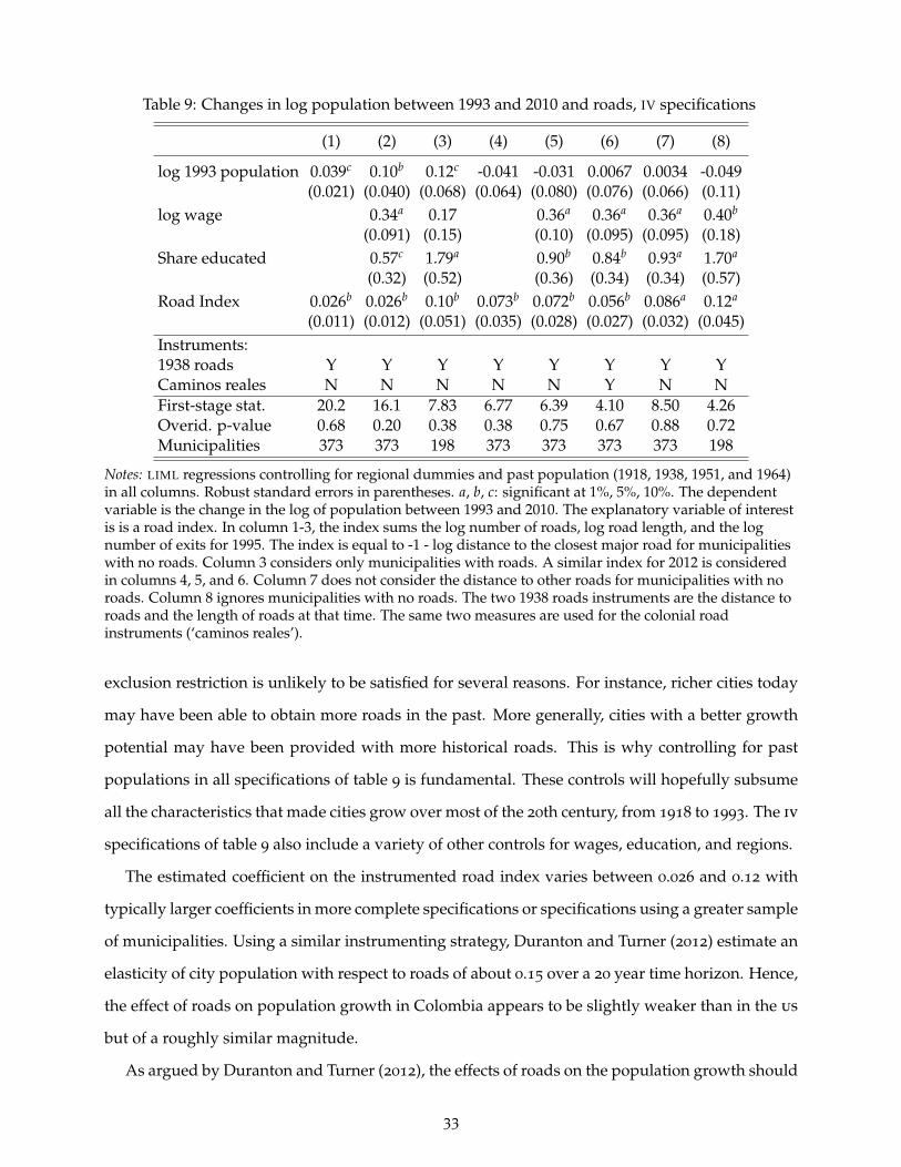
Table 9: Changes in log population between 1993 and 2010 and roads, IV specifications

(1) (2) (3) (4) (5) (6) (7) (8)

log 1993 population 0.039c 0.10b 0.12c -0.041 -0.031 0.0067 0.0034 -0.049(0.021) (0.040) (0.068) (0.064) (0.080) (0.076) (0.066) (0.11)

log wage 0.34a 0.17 0.36a 0.36a 0.36a 0.40b

(0.091) (0.15) (0.10) (0.095) (0.095) (0.18)Share educated 0.57c 1.79a 0.90b 0.84b 0.93a 1.70a

(0.32) (0.52) (0.36) (0.34) (0.34) (0.57)Road Index 0.026b 0.026b 0.10b 0.073b 0.072b 0.056b 0.086a 0.12a

(0.011) (0.012) (0.051) (0.035) (0.028) (0.027) (0.032) (0.045)Instruments:1938 roads Y Y Y Y Y Y Y YCaminos reales N N N N N Y N NFirst-stage stat. 20.2 16.1 7.83 6.77 6.39 4.10 8.50 4.26Overid. p-value 0.68 0.20 0.38 0.38 0.75 0.67 0.88 0.72Municipalities 373 373 198 373 373 373 373 198

Notes: LIML regressions controlling for regional dummies and past population (1918, 1938, 1951, and 1964)in all columns. Robust standard errors in parentheses. a, b, c: significant at 1%, 5%, 10%. The dependentvariable is the change in the log of population between 1993 and 2010. The explanatory variable of interestis is a road index. In column 1-3, the index sums the log number of roads, log road length, and the lognumber of exits for 1995. The index is equal to -1 - log distance to the closest major road for municipalitieswith no roads. Column 3 considers only municipalities with roads. A similar index for 2012 is consideredin columns 4, 5, and 6. Column 7 does not consider the distance to other roads for municipalities with noroads. Column 8 ignores municipalities with no roads. The two 1938 roads instruments are the distance toroads and the length of roads at that time. The same two measures are used for the colonial roadinstruments (‘caminos reales’).

exclusion restriction is unlikely to be satisfied for several reasons. For instance, richer cities today

may have been able to obtain more roads in the past. More generally, cities with a better growth

potential may have been provided with more historical roads. This is why controlling for past

populations in all specifications of table 9 is fundamental. These controls will hopefully subsume

all the characteristics that made cities grow over most of the 20th century, from 1918 to 1993. The iv

specifications of table 9 also include a variety of other controls for wages, education, and regions.

The estimated coefficient on the instrumented road index varies between 0.026 and 0.12 with

typically larger coefficients in more complete specifications or specifications using a greater sample

of municipalities. Using a similar instrumenting strategy, Duranton and Turner (2012) estimate an

elasticity of city population with respect to roads of about 0.15 over a 20 year time horizon. Hence,

the effect of roads on population growth in Colombia appears to be slightly weaker than in the us

but of a roughly similar magnitude.

As argued by Duranton and Turner (2012), the effects of roads on the population growth should

33

be interpreted in light of standard urban models where urban roads facilitate travel within the city.

This channel is arguably at play in us cities where interstate highways usually penetrate well inside

the central parts of those cities. This is less obvious that major roads play such a role in Colombia.

Road construction in Colombian cities sometimes involves the construction of a by-pass to avoid

too much through traffic. As a result, the main roads of Colombia might not be as important to

foster urban growth as in some other countries.

Another reason why roads might affect city population is through trade with other cities. In

Duranton (2015), I use the same approach as Duranton et al. (2014) and present evidence that roads

in Colombia foster trade. Cities with more roads export and import more, all else equal. While a

full exploration of the infrastructure-trade-population growth nexus would go beyond the scope

of this paper, preliminary steps can be taken by looking at the effects of market access on city

population growth.

What constitutes a good access to market is more complicated than it first seems. The reason

is that proximity to large cities implies a tradeoff. While large cities represent large markets with

many potential customers, they are also tougher markets for which the presence of more producers

will lead to lower prices. This occurs because of tougher price competition, the elimination of

weaker firms, or a simple market crowding effect.17 In practice, market access can be measured

through a simple market potential index that sums the gdps of a municipality’s neighbours,

discounting them by distance. Following Redding and Venables (2004), an alternative is to re-

constitute a theory-consistent measure of market access using trade data. In models of economic

geography in the tradition of Fujita et al. (1999), a simple gravity estimation of trade patterns allows

one to recover a theory-consistent measure of market access despite the absence of price data for

the goods being traded. This is the strategy followed in Duranton (2015). Here, I use both types of

measures. Because the effect of market access is not expected to be linear, especially for the more

ad-hoc market potential measures, I use both a log and its square in the regressions.

The results are reported in table 10. The first key feature that arises from this table is a negative

relationship between the true measure of market access used in columns 1-4 and city population

growth. When using a more ad-hoc measure of market potential in columns 5-8, the estimated ef-

fect is bell-shaped. This is likely to be a reflection of the faster growth of ‘suburban’ municipalities

17There is a large theoretical literature on market access. See Fujita, Krugman, and Venables (1999) for a starting point.

34

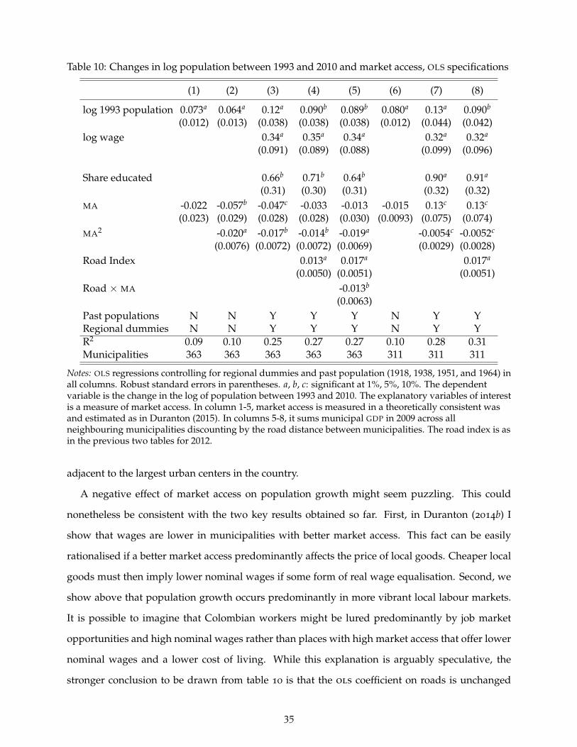
Table 10: Changes in log population between 1993 and 2010 and market access, OLS specifications

(1) (2) (3) (4) (5) (6) (7) (8)

log 1993 population 0.073a 0.064a 0.12a 0.090b 0.089b 0.080a 0.13a 0.090b

(0.012) (0.013) (0.038) (0.038) (0.038) (0.012) (0.044) (0.042)log wage 0.34a 0.35a 0.34a 0.32a 0.32a

(0.091) (0.089) (0.088) (0.099) (0.096)

Share educated 0.66b 0.71b 0.64b 0.90a 0.91a

(0.31) (0.30) (0.31) (0.32) (0.32)MA -0.022 -0.057b -0.047c -0.033 -0.013 -0.015 0.13c 0.13c

(0.023) (0.029) (0.028) (0.028) (0.030) (0.0093) (0.075) (0.074)MA2 -0.020a -0.017b -0.014b -0.019a -0.0054c -0.0052c

(0.0076) (0.0072) (0.0072) (0.0069) (0.0029) (0.0028)Road Index 0.013a 0.017a 0.017a

(0.0050) (0.0051) (0.0051)Road × MA -0.013b

(0.0063)Past populations N N Y Y Y N Y YRegional dummies N N Y Y Y N Y YR2 0.09 0.10 0.25 0.27 0.27 0.10 0.28 0.31Municipalities 363 363 363 363 363 311 311 311

Notes: OLS regressions controlling for regional dummies and past population (1918, 1938, 1951, and 1964) inall columns. Robust standard errors in parentheses. a, b, c: significant at 1%, 5%, 10%. The dependentvariable is the change in the log of population between 1993 and 2010. The explanatory variables of interestis a measure of market access. In column 1-5, market access is measured in a theoretically consistent wasand estimated as in Duranton (2015). In columns 5-8, it sums municipal GDP in 2009 across allneighbouring municipalities discounting by the road distance between municipalities. The road index is asin the previous two tables for 2012.

adjacent to the largest urban centers in the country.

A negative effect of market access on population growth might seem puzzling. This could

nonetheless be consistent with the two key results obtained so far. First, in Duranton (2014b) I

show that wages are lower in municipalities with better market access. This fact can be easily

rationalised if a better market access predominantly affects the price of local goods. Cheaper local

goods must then imply lower nominal wages if some form of real wage equalisation. Second, we

show above that population growth occurs predominantly in more vibrant local labour markets.

It is possible to imagine that Colombian workers might be lured predominantly by job market

opportunities and high nominal wages rather than places with high market access that offer lower

nominal wages and a lower cost of living. While this explanation is arguably speculative, the

stronger conclusion to be drawn from table 10 is that the ols coefficient on roads is unchanged

35

by the introduction of market access variables in the regression. This is a useful check on the

robustness of their effect and an indication that roads are likely to matter predominantly because

of local travel rather than inter-city trade.

From the broad exploration of the determinants of city growth conducted in this section, the

main takeaway result concerns to the importance of roads. There are further suggestions that

city roads matter because they facilitate travel within cities. Two secondary results relate to the

importance of natural resources, and particularly oil, and of local criminality. Interestingly, two of

these three results reinforce the conclusions drawn from section 4 highlighting the importance of

viewing Colombian cities as local labour markets. This is because oil is a key determinant of the

demand for labour in the municipalities where it can be found and because easier travel within a

city will benefit to commuters going to work.

6. Long-run growth of cities in Colombia

Although a lot of the municipal data used so is for the late 20th and early 21st century, municipal

population data in Colombia is available since 1843. The roads instruments used above also go

back to the colonial (or even pre-colonial) era. Together with information about resources and

natural geography, this allows us to have a peek at the long-run determinants of urban growth in

Colombia. Given data limitations, this analysis of the long-run growth of Colombian cities should

be viewed as even more tentative than the analysis conducted so far.

Panel a of table 11 report results for population growth between 1938 and 2010. Because past

populations dating back to 1843 (used as controls in columns 2-8) are not available for many

(smaller) municipalities, the sample size here is about 30% smaller than in the tables above. The

specifications in panel b examine an even longer time period, 1870-2010 for columns 1-5 and

1843-2010 for columns 6-8. As Colombia became independent in 1819 and 1843 is arguably its

first usable census, these specifications cover most of the history of modern Colombia.

Four main results emerge. The first regards mean-reversion in population across municipalities.

While there is evidence above of some population divergence over 1993-2010, there is neither

convergence nor divergence over the longer time period of 1938 to 2010. Interestingly, there is

strong mean-reversion if we go back to 1870 or 1843. These results are consistent with the notion

that the Colombian population first spread across the country with the expansion of its agricultural

36

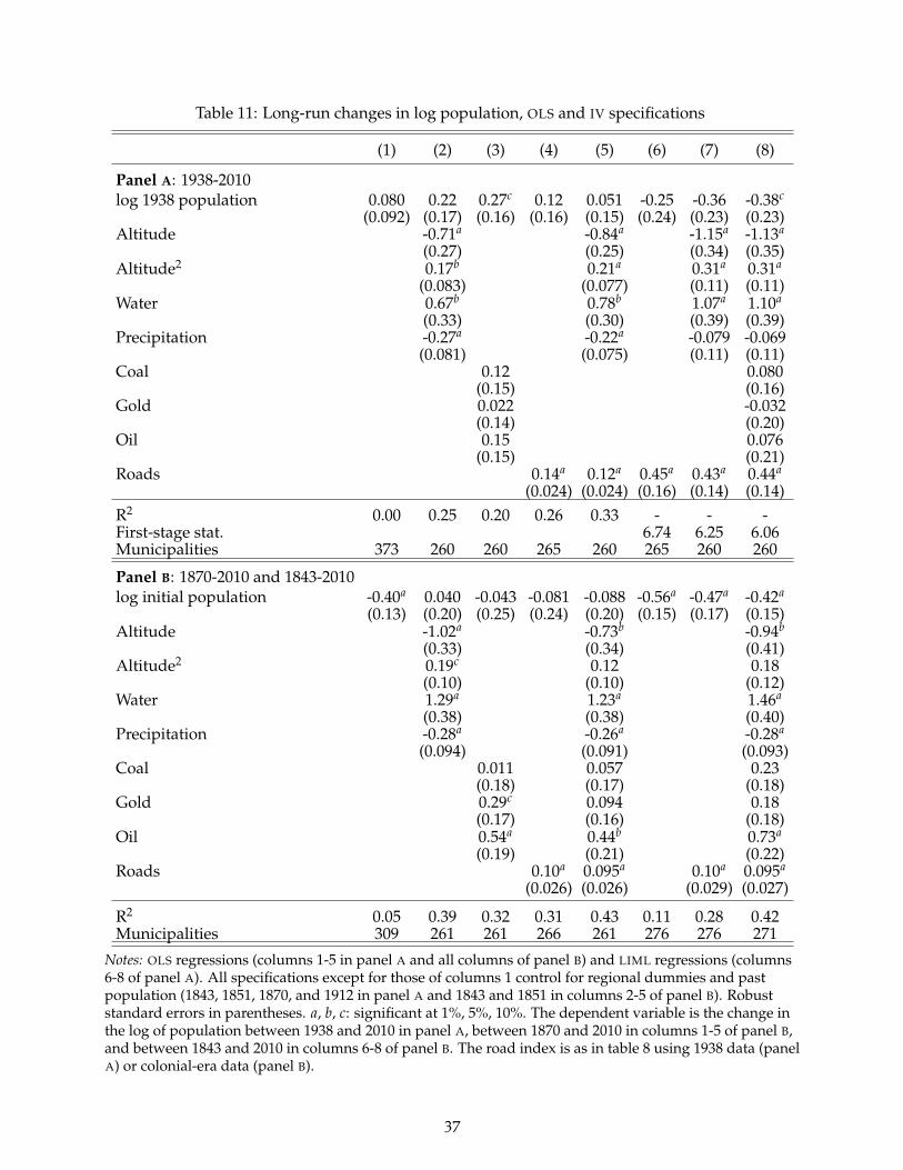
Table 11: Long-run changes in log population, OLS and IV specifications

(1) (2) (3) (4) (5) (6) (7) (8)

Panel A: 1938-2010log 1938 population 0.080 0.22 0.27c 0.12 0.051 -0.25 -0.36 -0.38c

(0.092) (0.17) (0.16) (0.16) (0.15) (0.24) (0.23) (0.23)Altitude -0.71a -0.84a -1.15a -1.13a

(0.27) (0.25) (0.34) (0.35)Altitude2 0.17b 0.21a 0.31a 0.31a

(0.083) (0.077) (0.11) (0.11)Water 0.67b 0.78b 1.07a 1.10a

(0.33) (0.30) (0.39) (0.39)Precipitation -0.27a -0.22a -0.079 -0.069

(0.081) (0.075) (0.11) (0.11)Coal 0.12 0.080

(0.15) (0.16)Gold 0.022 -0.032

(0.14) (0.20)Oil 0.15 0.076

(0.15) (0.21)Roads 0.14a 0.12a 0.45a 0.43a 0.44a

(0.024) (0.024) (0.16) (0.14) (0.14)R2 0.00 0.25 0.20 0.26 0.33 - - -First-stage stat. 6.74 6.25 6.06Municipalities 373 260 260 265 260 265 260 260

Panel B: 1870-2010 and 1843-2010log initial population -0.40a 0.040 -0.043 -0.081 -0.088 -0.56a -0.47a -0.42a

(0.13) (0.20) (0.25) (0.24) (0.20) (0.15) (0.17) (0.15)Altitude -1.02a -0.73b -0.94b

(0.33) (0.34) (0.41)Altitude2 0.19c 0.12 0.18

(0.10) (0.10) (0.12)Water 1.29a 1.23a 1.46a

(0.38) (0.38) (0.40)Precipitation -0.28a -0.26a -0.28a

(0.094) (0.091) (0.093)Coal 0.011 0.057 0.23

(0.18) (0.17) (0.18)Gold 0.29c 0.094 0.18

(0.17) (0.16) (0.18)Oil 0.54a 0.44b 0.73a

(0.19) (0.21) (0.22)Roads 0.10a 0.095a 0.10a 0.095a

(0.026) (0.026) (0.029) (0.027)

R2 0.05 0.39 0.32 0.31 0.43 0.11 0.28 0.42Municipalities 309 261 261 266 261 276 276 271

Notes: OLS regressions (columns 1-5 in panel A and all columns of panel B) and LIML regressions (columns6-8 of panel A). All specifications except for those of columns 1 control for regional dummies and pastpopulation (1843, 1851, 1870, and 1912 in panel A and 1843 and 1851 in columns 2-5 of panel B). Robuststandard errors in parentheses. a, b, c: significant at 1%, 5%, 10%. The dependent variable is the change inthe log of population between 1938 and 2010 in panel A, between 1870 and 2010 in columns 1-5 of panel B,and between 1843 and 2010 in columns 6-8 of panel B. The road index is as in table 8 using 1938 data (panelA) or colonial-era data (panel B).

37

frontier but then, in the more recent past, started to concentrate more in its largest cities. As already

noted, this movement of spatial concentration goes well beyond the emerging primacy of Bogotá

in the Colombian urban system.

Second, there is strong evidence of a role for natural geography in the long-run. This role

is limited to non-existent for the recent past, as shown in table 7. Since 1938 and prior to this,

the availability of water matters a lot. There is a also a negative association between long-run

population growth and precipitation. Interestingly, the effect of altitude is non-linear. Population

growth is minimum in panel a at about 2,000 metres. Even for high-altitude cities like Bogotá

and Tunja (at 2,600 and 2,800 meters respectively) the effect remains strongly negative relative to

coastal cities.

Third, the evidence in favour of natural resources is mixed. As we saw above, among natural

resources only oil appears to play a role over 1993-2010. I do not observe any effect of any natural

resource over 1938-2010. Over an even longer time horizon, there is evidence of an association with

the presence of oil, and perhaps gold. This result regarding oil since 1870 or even 1843 is arguably

spurious as the Colombian oil industry has been active for no more than 40 years. It illustrates the

limitations of the exercise conducted here. These positive coefficients on oil are probably due to

the peripheral locations of oil fields in Colombia. Hence, positive coefficients on oil are likely to

capture the long-run patterns of settlement of the country.

Finally, we measure a positive effect of roads. For 1938-2010 population growth, the ols elastic-

ity with respect to 1938 roads is slightly above 0.10. When instrumenting 1938 roads with colonial

roads, the estimated elasticity of population with respect to roads jumps to between 0.40 and 0.50.

This increase must be in part caused by the poor measurement of 1938 roads that is improved

by instrumenting. In panel b, colonial roads are directly used as an explanatory variable. They

are significant again with a coefficient of about 0.10. Again, measurement issues prevent us from

reading too much into these magnitudes but it remains that roads appear to exert a long-run effect

on population growth in Colombia.

7. Conclusion

While extant research on city growth mostly focuses on one determinant or another, this paper has

taken a broader and more comprehensive approach to this question by considering a broad array

of determinants of city growth. The main potential drawback of doing this is that the effect of each

38

factor may not be as persuasively identified as in the best ‘one-factor’ studies. Although it must be

acknowledged that the causal interpretation of some of the results derived here remains tentative,

I have tried to minimize this problem by following the best practice defined by leading one-factor

studies of city growth.

Against this possible drawback, the main benefit of the approach taken here is threefold. First,

the whole is more than the sum of its parts. Having established that labour mobility across cities

in Colombia is far from perfect allowed us to assess how the Colombian population gradually

moves to cities offering higher wages. In turn, we could trace these higher wages back to labour

market shocks. In turn, this suggests that Colombian cities are best characterised as local labour

markets. Those that prosper and demand more labour grow in population. Second, this approach

also allows for a more nuanced appreciation of city growth. While being a dynamic local labour

market is the first-order determinant of city growth, it is not the only one: education, crime, and

the ease of travel also play a role. Third, some of the key conclusions can be supported by a

variety of results instead of only one. For instance, the fundamental role of cities as labour markets

could be evidenced directly through wages and labour market shocks but also indirectly through

the attenuation of the effect of city education when controlling for wages or the general lack of

evidence about amenities.

References

Aiura, Hiroshi and Yasuhiro Sato. 2014. A model of urban demography. Canadian Journal ofEconomics 47(3):981–1009.

Alonso, William. 1964. Location and Land Use; Toward a General Theory of Land Rent. Cambridge, ma:Harvard University Press.

Bartik, Timothy. 1991. Who Benefits from State and Local Economic Development Policies? Kalamazoo(mi): W.E. Upjohn Institute for Employment Research.

Beaudry, Paul, David A. Green, and Benjamin M. Sand. 2014. Spatial equilibrium with unemploy-ment and wage bargaining: Theory and estimation. Journal of Urban Economics 79(1):2–19.

Bushnell, David. 1993. The Making of Modern Colombia: A Nation in Spite of Itself. Berkeley (ca):University of California Press.

Carlino, Gerald A. and Albert Saiz. 2008. Beautiful city: Leisure amenities and urban growth. FRBof Philadelphia Working Paper No. 08-22.

Cheshire, Paul C. and Stefano Magrini. 2006. Population growth in european cities: weathermatters-but only nationally. Regional Studies 40(1):23–37.

39

da Mata, Daniel, Uwe Deichmann, J. Vernon Henderson, Somik V. Lall, and Hyoung Gun Wang.2007. Determinants of city growth in Brazil. Journal of Urban Economics 62(2):252–272.

De la Roca, Jorge and Diego Puga. 2012. The dynamic earnings premium of dense cities. Processed,cemfi and imdea Social Sciences.

Deliktas, Ertugrul, A. Özlem Önder, and Metin Karadag. 2013. The size distribution of cities anddeterminants of city growth in Turkey. European Planning Studies 21(2):251–263.

Desmet, Klaus and J. Vernon Henderson. 2015. The geography of development within countries.In Gilles Duranton, Vernon Henderson, and Williman Strange (eds.) Handbook of Regional andUrban Economics, volume 5B. Amsterdam: Elsevier, 1457–1517.

Duranton, Gilles. 2007. Urban evolutions: The fast, the slow, and the still. American EconomicReview 97(1):197–221.

Duranton, Gilles. 2013a. Delineating metropolitan areas: Measuring spatial labour market net-works through commuting patterns. Mimeographed, Wharton School, University of Pennsylva-nia.

Duranton, Gilles. 2013b. The growth of metropolitan areas in the United States. In Susan Wachterand Kimberly Zeuli (eds.) Revitalizing American Cities. Philadelphia: University of PennsylvaniaPress, 26–44.

Duranton, Gilles. 2014a. Growing through cities in developing countries. World Bank ResearchObserver 39(1):39–73.

Duranton, Gilles. 2014b. Agglomeration effects in Colombia. Processed, Wharton School, Univer-sity of Pennsylvania.

Duranton, Gilles. 2015. Roads and trade in Colombia. Economics of Transportation 4:forthcoming.

Duranton, Gilles, Peter M. Morrow, and Matthew A. Turner. 2014. Roads and trade: Evidence fromthe us. Review of Economic Studies 81(2):681–724.

Duranton, Gilles and Diego Puga. 2000. Diversity and specialisation in cities: Why, where andwhen does it matter? Urban Studies 37(3):533–555.

Duranton, Gilles and Diego Puga. 2014. The growth of cities. In Philippe Aghion and StevenDurlauf (eds.) Handbook of Economic Growth, volume 2. Amsterdam: North-Holland, 781–853.

Duranton, Gilles and Matthew A. Turner. 2012. Urban growth and transportation. Review ofEconomic Studies 79(4):1407–1440.

Eeckhout, Jan. 2004. Zipf’s law for (all) cities. American Economic Review 94(5):1429–1451.

Fujita, Masahisa, Paul R. Krugman, and Anthony J. Venables. 1999. The Spatial Economy: Cities,Regions, and International Trade. Cambridge (ma): mit Press.

García-López, Miquel-Ángel, Adelheid Holl, and Elisabet Viladecans-Marsal. 2014. Infrastruc-ture and cities: The incidence of new highways on urban growth. Processed, Universitat deBarcelona.

Glaeser, Edward L. 2011. Triumph of the city: How our greatest invention makes us richer, smarter,greener, healthier and happier. New York (NY): Macmillan.

40

Glaeser, Edward L., Heidi Kallal, José A. Scheinkman, and Andrei Shleifer. 1992. Growth in cities.Journal of Political Economy 100(6):1126–1152.

Glaeser, Edward L., Jed Kolko, and Albert Saiz. 2001. Consumer city. Journal of Economic Geography1(1):27–50.

Glaeser, Edward L., Giacomo A. M. Ponzetto, and Kristina Tobio. 2014. Cities, skills and regionalchange. Regional Studies 48(1):7–43.

Glaeser, Edward L. and Albert Saiz. 2004. The rise of the skilled city. Brookings-Wharton Papers onUrban Affairs 5(0):47–94.

Glaeser, Edward L., José A. Scheinkman, and Andrei Shleifer. 1995. Economic growth in a cross-section of cities. Journal of Monetary Economics 36(1):117–143.

Head, Keith and Thierry Mayer. 2004. The empirics of agglomeration and trade. In Vernon Hen-derson and Jacques-François Thisse (eds.) Handbook of Regional and Urban Economics, volume 4.Amsterdam: North-Holland, 2609–2669.

Henderson, J. Vernon and Anthony J. Venables. 2009. The dynamics of city formation. Review ofEconomic Dynamics 39(2):233–254.

Ioannides, Yannis and Spyros Skouras. 2013. US city size distribution: Robustly Pareto, but onlyin the tail. Journal of Urban Economics 73(1):18–29.

Jedwab, Rémi, Luc Christiaensen, and Marina Gindelsky. 2014. Demography, urbanization anddevelopment: Rural push, urban pull and... urban push? Processed, George WashingtonUniversity.

Jedwab, Rémi and Dietrich Vollrath. 2015. The mortality transition, Malthusian dynamics and therise of poor megacities. Processed, George Washington University.

Meisel Roca, Adolfo and Gerson Javier Pérez. 2012. Las ciudades colombianas y sus attractivos.Report for the Urban Development Division of the National Planning Ministry (dnp-ddu).

Mills, Edwin S. 1967. An aggregative model of resource allocation in a metropolitan area. AmericanEconomic Review (Papers and Proceedings) 57(2):197–210.

Moretti, Enrico. 2004. Estimating the social return to higher education: Evidence from longitudinaland repeated cross-sectional data. Journal of Econometrics 121(1):175–212.

Muth, Richard F. 1969. Cities and Housing. Chicago: University of Chicago Press.

Rappaport, Jordan. 2007. Moving to nice weather. Regional Science and Urban Economics 37(3):375–398.

Redding, Stephen and Anthony J. Venables. 2004. Economic geography and international inequal-ity. Journal of International Economics 62(1):63–82.

Redding, Stephen J. and Daniel M. Sturm. 2008. The costs of remoteness: Evidence from Germandivision and reunification. American Economic Review 98(5):1766–1797.

Redding, Stephen J. and Matthew A. Turner. 2015. Transportation costs and the spatial organiza-tion of economic activity. In Gilles Duranton, Vernon Henderson, and William C. Strange (eds.)Handbook of Regional and Urban Economics, volume 5B. Amsterdam: Elsevier, 1339–1398.

41

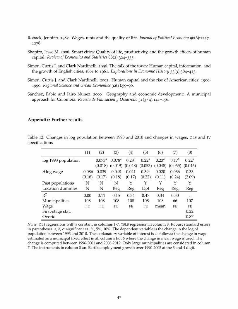
Roback, Jennifer. 1982. Wages, rents and the quality of life. Journal of Political Economy 90(6):1257–1278.

Shapiro, Jesse M. 2006. Smart cities: Quality of life, productivity, and the growth effects of humancapital. Review of Economics and Statistics 88(2):324–335.

Simon, Curtis J. and Clark Nardinelli. 1996. The talk of the town: Human capital, information, andthe growth of English cities, 1861 to 1961. Explorations in Economic History 33(3):384–413.

Simon, Curtis J. and Clark Nardinelli. 2002. Human capital and the rise of American cities: 1900-1990. Regional Science and Urban Economics 32(1):59–96.

Sánchez, Fabio and Jairo Nuñez. 2000. Geography and economic development: A municipalapproach for Colombia. Revista de Planeación y Desarrollo 31(3/4):141–156.

Appendix: Further results

Table 12: Changes in log population between 1993 and 2010 and changes in wages, OLS and IV

specifications

(1) (2) (3) (4) (5) (6) (7) (8)

log 1993 population 0.073a 0.078a 0.23a 0.22a 0.23a 0.17b 0.22a

(0.018) (0.019) (0.048) (0.053) (0.048) (0.065) (0.046)∆ log wage -0.086 0.039 0.048 0.041 0.39c 0.020 0.066 0.33

(0.18) (0.17) (0.18) (0.17) (0.22) (0.11) (0.24) (2.09)Past populations N N N Y Y Y Y YLocation dummies N N Reg Reg Dpt Reg Reg Reg

R2 0.00 0.11 0.15 0.34 0.47 0.34 0.30 .Municipalities 108 108 108 108 108 108 66 107Wage FE FE FE FE FE mean FE FE

First-stage stat. 0.22Overid 0.87

Notes: OLS regressions with a constant in columns 1-7. TSLS regression in column 8. Robust standard errorsin parentheses. a, b, c: significant at 1%, 5%, 10%. The dependent variable is the change in the log ofpopulation between 1993 and 2010. The explanatory variable of interest is as follows: the change in wageestimated as a municipal fixed effect in all columns but 6 where the change in mean wage is used. Thechange is computed between 1996-2001 and 2008-2012. Only large municipalities are considered in column7. The instruments in column 8 are Bartik employment growth over 1990-2005 at the 3 and 4 digit.

42

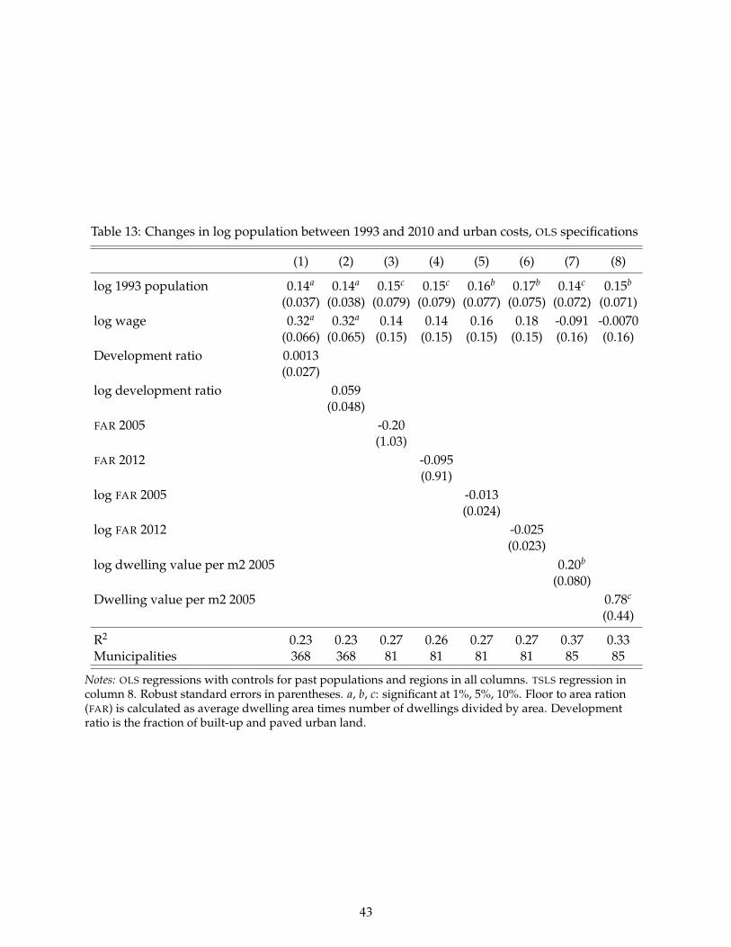
Table 13: Changes in log population between 1993 and 2010 and urban costs, OLS specifications

(1) (2) (3) (4) (5) (6) (7) (8)

log 1993 population 0.14a 0.14a 0.15c 0.15c 0.16b 0.17b 0.14c 0.15b

(0.037) (0.038) (0.079) (0.079) (0.077) (0.075) (0.072) (0.071)log wage 0.32a 0.32a 0.14 0.14 0.16 0.18 -0.091 -0.0070

(0.066) (0.065) (0.15) (0.15) (0.15) (0.15) (0.16) (0.16)Development ratio 0.0013

(0.027)log development ratio 0.059

(0.048)FAR 2005 -0.20

(1.03)FAR 2012 -0.095

(0.91)log FAR 2005 -0.013

(0.024)log FAR 2012 -0.025

(0.023)log dwelling value per m2 2005 0.20b

(0.080)Dwelling value per m2 2005 0.78c

(0.44)

R2 0.23 0.23 0.27 0.26 0.27 0.27 0.37 0.33Municipalities 368 368 81 81 81 81 85 85

Notes: OLS regressions with controls for past populations and regions in all columns. TSLS regression incolumn 8. Robust standard errors in parentheses. a, b, c: significant at 1%, 5%, 10%. Floor to area ration(FAR) is calculated as average dwelling area times number of dwellings divided by area. Developmentratio is the fraction of built-up and paved urban land.

43

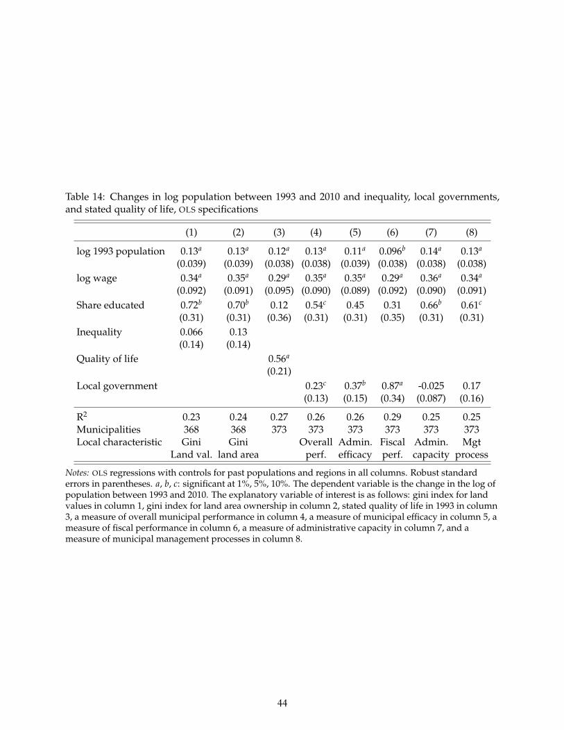
Table 14: Changes in log population between 1993 and 2010 and inequality, local governments,and stated quality of life, OLS specifications

(1) (2) (3) (4) (5) (6) (7) (8)

log 1993 population 0.13a 0.13a 0.12a 0.13a 0.11a 0.096b 0.14a 0.13a

(0.039) (0.039) (0.038) (0.038) (0.039) (0.038) (0.038) (0.038)log wage 0.34a 0.35a 0.29a 0.35a 0.35a 0.29a 0.36a 0.34a

(0.092) (0.091) (0.095) (0.090) (0.089) (0.092) (0.090) (0.091)Share educated 0.72b 0.70b 0.12 0.54c 0.45 0.31 0.66b 0.61c

(0.31) (0.31) (0.36) (0.31) (0.31) (0.35) (0.31) (0.31)Inequality 0.066 0.13

(0.14) (0.14)Quality of life 0.56a

(0.21)Local government 0.23c 0.37b 0.87a -0.025 0.17

(0.13) (0.15) (0.34) (0.087) (0.16)

R2 0.23 0.24 0.27 0.26 0.26 0.29 0.25 0.25Municipalities 368 368 373 373 373 373 373 373Local characteristic Gini Gini Overall Admin. Fiscal Admin. Mgt

Land val. land area perf. efficacy perf. capacity process

Notes: OLS regressions with controls for past populations and regions in all columns. Robust standarderrors in parentheses. a, b, c: significant at 1%, 5%, 10%. The dependent variable is the change in the log ofpopulation between 1993 and 2010. The explanatory variable of interest is as follows: gini index for landvalues in column 1, gini index for land area ownership in column 2, stated quality of life in 1993 in column3, a measure of overall municipal performance in column 4, a measure of municipal efficacy in column 5, ameasure of fiscal performance in column 6, a measure of administrative capacity in column 7, and ameasure of municipal management processes in column 8.

44