Munich Personal RePEc Archive

The decline in Italian productivity: a

study in estimation of Total Factor

Productivity with panel cointegration

methods

Fachin, Stefano and Gavosto, Andrea

Faculty of Statistics, University of Rome ”La Sapienza”

7 May 2007

Online at https://mpra.ub.uni-muenchen.de/26972/

MPRA Paper No. 26972, posted 26 Nov 2010 04:11 UTC

The decline in Italian Labour Productivity:A Study in Estimation of Total Factor

Productivitywith Panel Cointegration Methods

Stefano FachinFaculty of Statistics, Università di Roma �La Sapienza�

Andrea GavostoFondazione Giovanni Agnelli

Abstract

The main aim of this paper is to propose a method for obtaining esti-mates of Total Factor Productivity (TFP) trends (i) free from the restrictiveassumptions needed by traditional growth accounting and (ii) requiring onlydata on inputs and output �ows. The approach proposed relies on recentdevelopments in the analysis of non-stationary dependent panels. The ap-plication to the Italian economy for the period 1981-2004, consistently withthose obtained through traditional growth accounting methods, supports theview that the decline in Italian labour productivity has been mostly due toa widespread fall in TFP growth. A simple regression points as main causesof this fall the completion of a factor reallocation process among industriesand capital types.

Keywords: Total Factor Productivity, Productivity Slowdown, Italy,Panel Cointegration.

Revised December 2008

1

1 Introduction1

The growth of value added per worker (henceforth labour productivity) inItaly since the late 1990�s has been abysmal, the poorest in Europe alongwith Spain2: over the period 1995-20043 the annual average growth has beenjust 1.3%, with a falling trend ( 0.5% per year in 2000-2004). For a com-parison, in the USA the growth, about 2.5% a year in 1995-2001, increasedto 4% a year in 2001-2004. In fact, the Governor of the Federal ReserveB.S. Bernanke recently stated that �Almost certainly, the most importanteconomic development in the United States in the past decade has been thesustained increase in the rate of growth of labor productivity, or output perhour of work.� (Bernanke, 2005). As stressed by Bernanke, labour produc-tivity growth is important not only in the long-run, as the force shapingliving standards, but also in the short-run, as one of the determinants ofoutput and employment growth. Hence, understanding the causes of thislabour productivity slowdown is a matter of great importance4.

Formally we can put the question as follows: is the productivity slow-down due to a movement along an isoquant or, rather, to a shift of the iso-quant? The former may occur as a consequence of a fall in capital intensity,perhaps linked to a change in relative factor prices; the latter, of a decline intotal factor productivity (TFP). Declining TFP will coeteris paribus implielower value added per worker, i.e. labour productivity, also. The answer isclearly highly relevant from a policy perspective. In fact, should the pro-ductivity slowdown (consistently with the observed upsurge in employmentin the last decade), simply be a consequence of a re-adjustment in the fac-tor mix, there should be no concern. The phenomenon could be seen as amarket-driven reaction to an excessive capital intensity of the past. On theother hand, if the problem lies in total factor productivity, two possibilitiesarise: either the slowdown re�ects the exhaustion of the �quality adjust-

1The �rst author acknowledges �nancial support from University of Rome �LaSapienza� and MIUR. We would like to thank Riccardo Cristadoro and Andrea Bran-dolini for kindly providing the Bank of Italy Capacity Utilisation and Human Capitaldata, Carlo Altomonte and participants at the Turin February 2007 CNR Meeting of in-ternational economics and Brescia 2008 AIEL conference for very helpful comments andsuggestions. The usual disclaimers apply.

2See inter alia, Daveri and Jona-Lasinio (2005). For a very recent assessment based onthe Groeningen dataset see Conference Board (2007).

3Data limitations for the Capital stock, a key variable of our study, prevent us fromconsidering the period after 2004.

4Concern for analogous productiviy slowdown events from the policymaker perspectivecan be found, e.g., in Dolman, Lu and Rahman (2005) for the Australian economy, andin Centraal Planbureau (1998) for the Dutch economy.

2

ment� component, linked to reallocation across industries, labour skills, orcapital vintages and types (see the literature dating back to Denison, 1967,and Matthews et al., 1982); or it re�ects a decline in pure (disembodied)technological progress, due, say, to fewer research, development and inno-vation. The latter hypothesis is of particular concern to policy-makers, asit would result in a prolonged competitiveness gap of the Italian indus-try vis-à-vis other countries, especially within the single currency area. Anumber of studies have tackled the question: see for instance Bassanetti,Iommi, Jona-Lasinio and Zollino (2004), henceforth BIJZ, and Daveri andJona-Lasinio (2005). The common conclusion is that most of the decline inproductivity since 1995 is due to the decline in TFP. Although there hasbeen some reduction in capital deepening in the period, this has been com-pensated by an increase in the share of capital in the economy-wide valueadded. For instance, Daveri and Jona-Lasinio (2005) estimate that 1 outof the 1.2 percentage points reduction in labour productivity growth withrespect to the period 1980-95 is accounted for by the decline in TFP in theoverall economy.

Hence, TFP estimation becomes crucial. The debate on this issue wasrecently revived in a series of papers (see Kee, 2004, and the references citedtherein). However, these papers are mostly addressed at comparing the so-called primal and dual growth accounting methods, while the key point isthat, as put by Stiroh (2002): �While growth accounting provides a valuableand well-tested means for understanding the proximate sources of growth,additional tests are needed to corroborate those results� (p. 1559). In fact,growth accounting relies on the assumptions of constant returns to scale andperfect competition in both the products and factors markets, hypothesisrespectively not guaranteed and very unlikely to hold. Kee (2004) adds animportant contribution to the literature by developing a more general ap-proach based upon a structural model requiring neither perfect competitionnor constant returns to scale. Although more general than standard growthaccounting, his approach restricts the degree of market power to be constantover time. Further, the analysis carried out on �rst di¤erences, thus leavingopen the question on long-run TFP trends.

Summing up, a method for obtaining estimates of TFP long-run trendswithout overly restrictive assumptions on technology and market structureseems still to be missing. In this paper we address this issue. More pre-cisely, applying recent non-stationary panel techniques we will examine re-cent labour productivity patterns in the Italian manufacturing industry andobtain estimates of the underlying aggregate TFP trend valid under verygeneral hypotheses on the di¤usion of technical progress across industries.

3

Using these estimates we will then (i) estimate a simple model relating TFPgrowth to factors reallocation across industries and factor quality dynam-ics, and (ii) estimate disaggregate production functions. As we will see inmore detail below, a non negligible advantage of the proposed approach isthat, di¤erently from both standard growth accounting and Kee�s structuralapproach, no information on the rental price of capital is required.

The paper is organised as follows: we shall �rst examine the data (section1), then move to modelling issues (section 2, with the technical details of thebootstrap algorithms employed described in the Appendix). Finally, someconclusions will be drawn (section 3).

2 What do the Disaggregate Data Say? Produc-

tivity, Output, Labour and Capital Trends in

Italian Manufacturing Industries, 1981-2004

First of all, let us review the data evidence. Since we will estimate a sin-gle TFP trend we will limit the analysis to the Subsections included inthe NACE Sections �Mining and Quarrying� (C), �Manufacturing� (D) and�Electricity, Gas and Water Supply� (E, henceforth �Utilities�; the NACEclassi�cation with all the abbreviations used as well as, for reference�s sake,the average value added shares, are reported in the Data Appendix). Agri-culture and Market Services, technically far too heterogenous, and, as faras the latter is concerned, plagued by serious productivity measurementproblems, have been excluded. As data on Capital are available from 1980,a peak year according to almost all dating methods (Bruno and Otranto,2003), until 2004, we will examine the period 1981-2004. All details on thedata sources and de�nitions are also reported in the Data Appendix.

The log plots of the aggregate level trends (Fig. ??, left column) tellan apparently rather clear story: Labour Productivity (measured by theValue Added/labour inputs ratio), Value Added and Capital/Labour ratio(rescaled to account for capacity utilisation) grew more or less steadily, whileemployment (measured in terms of full time equivalent employees) followedan opposite, declining trend. However, looking at the right column of thesame �gure we can notice that in fact the rates of growth of both labourproductivity and capital/labour ratio kept falling throughout the period,while, on the contrary, employment growth accelerated over the last yearsof the sample. Thus, the aggregate evidence seems to suggest a declinein capital deepening causing the labour productivity slowdown and accel-eration in labour demand (formally, a movement along an isoquant of the

4

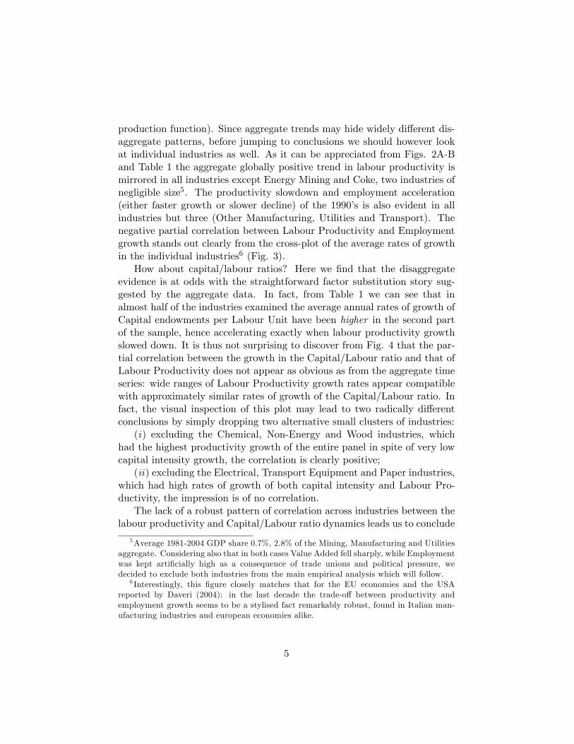
production function). Since aggregate trends may hide widely di¤erent dis-aggregate patterns, before jumping to conclusions we should however lookat individual industries as well. As it can be appreciated from Figs. 2A-Band Table 1 the aggregate globally positive trend in labour productivity ismirrored in all industries except Energy Mining and Coke, two industries ofnegligible size5. The productivity slowdown and employment acceleration(either faster growth or slower decline) of the 1990�s is also evident in allindustries but three (Other Manufacturing, Utilities and Transport). Thenegative partial correlation between Labour Productivity and Employmentgrowth stands out clearly from the cross-plot of the average rates of growthin the individual industries6 (Fig. 3).

How about capital/labour ratios? Here we �nd that the disaggregateevidence is at odds with the straightforward factor substitution story sug-gested by the aggregate data. In fact, from Table 1 we can see that inalmost half of the industries examined the average annual rates of growth ofCapital endowments per Labour Unit have been higher in the second partof the sample, hence accelerating exactly when labour productivity growthslowed down. It is thus not surprising to discover from Fig. 4 that the par-tial correlation between the growth in the Capital/Labour ratio and that ofLabour Productivity does not appear as obvious as from the aggregate timeseries: wide ranges of Labour Productivity growth rates appear compatiblewith approximately similar rates of growth of the Capital/Labour ratio. Infact, the visual inspection of this plot may lead to two radically di¤erentconclusions by simply dropping two alternative small clusters of industries:

(i) excluding the Chemical, Non-Energy and Wood industries, whichhad the highest productivity growth of the entire panel in spite of very lowcapital intensity growth, the correlation is clearly positive;

(ii) excluding the Electrical, Transport Equipment and Paper industries,which had high rates of growth of both capital intensity and Labour Pro-ductivity, the impression is of no correlation.

The lack of a robust pattern of correlation across industries between thelabour productivity and Capital/Labour ratio dynamics leads us to conclude

5Average 1981-2004 GDP share 0.7%, 2.8% of the Mining, Manufacturing and Utilitiesaggregate. Considering also that in both cases Value Added fell sharply, while Employmentwas kept arti�cially high as a consequence of trade unions and political pressure, wedecided to exclude both industries from the main empirical analysis which will follow.

6 Interestingly, this �gure closely matches that for the EU economies and the USAreported by Daveri (2004): in the last decade the trade-o¤ between productivity andemployment growth seems to be a stylised fact remarkably robust, found in Italian man-ufacturing industries and european economies alike.

5

that the simple factor substitution story suggested by the aggregate data isin fact inadequate. Did a shift of the isoquant took place then? To answer tothis question a careful analysis of total factor productivity trends is required.

Before moving to this task, we conclude this exploratory section exam-ining the time series properties of the series. The general impression isobviously of non-stationarity; given the small time sample in order to run aformal test we need to use a panel unit root test, which, since the units aredependent, must be robust to cross-correlation. A procedure which appearsto be both simple and powerful is Pesaran (2006) CIPS test, which is essen-tially an average of the Dickey-Fuller tests computed for the individual units(i.e., the popular test by Im, Pesaran and Shin, 2003) augmented with thecross-section means. The results, reported in Table 3, are largely in favourof the unit root hypothesis, thus con�rming the graphical evidence.

6

Figure 1: Fig. 1. Mining, Manufacturing and Utilities, 1981-2004. Topto bottom: Value Added per Labour Unit, Value Added, Employment inLabour Units, Gross Capital per Labour Unit. Left: logs; right: � log.Value Added at 1995 prices; Capital at 1995 prices rescaled by the Bank ofItaly Capacity Utilisation Index .

7

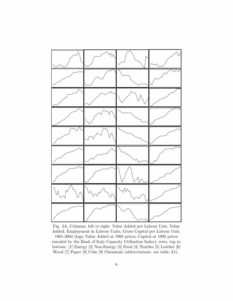
Fig. 2A. Columns, left to right: Value Added per Labour Unit, ValueAdded, Employment in Labour Units, Gross Capital per Labour Unit,1981-2004 (logs; Value Added at 1995 prices; Capital at 1995 pricesrescaled by the Bank of Italy Capacity Utilisation Index); rows, top tobottom: [1] Energy [2] Non-Energy [3] Food [4] Textiles [5] Leather [6]Wood [7] Paper [8] Coke [9] Chemicals (abbreviations: see table A1).

8

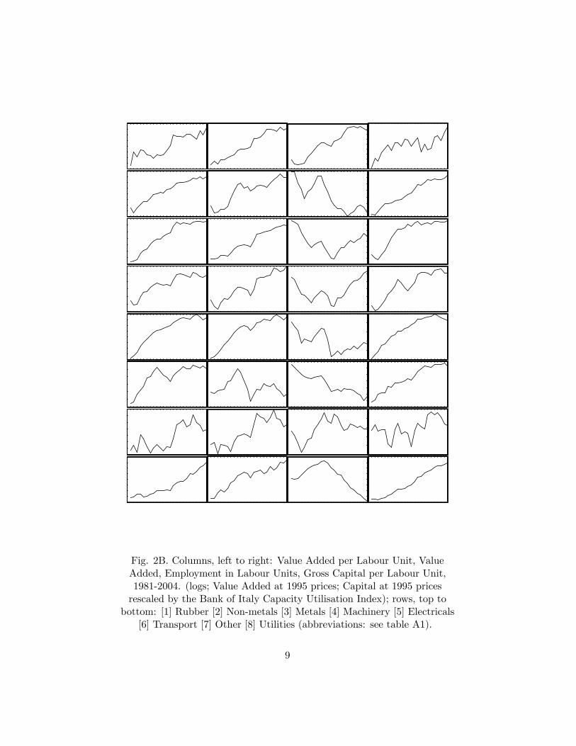
Fig. 2B. Columns, left to right: Value Added per Labour Unit, ValueAdded, Employment in Labour Units, Gross Capital per Labour Unit,1981-2004. (logs; Value Added at 1995 prices; Capital at 1995 pricesrescaled by the Bank of Italy Capacity Utilisation Index); rows, top to

bottom: [1] Rubber [2] Non-metals [3] Metals [4] Machinery [5] Electricals[6] Transport [7] Other [8] Utilities (abbreviations: see table A1).

9

Fig. 3. Annual average rates of growth�100 of Value Added per LabourUnit (VA/L) and Labour Units (L), 1981-2004 (Industries abbreviations:

see table A1).

10

Figure 2: Fig. 4. Annual average rates of growth�100 of Value Addedper Labour Unit (VA/L) and Capital per Labour Unit (K/L), 1981-2004(Industries abbreviations: see table A1).

11

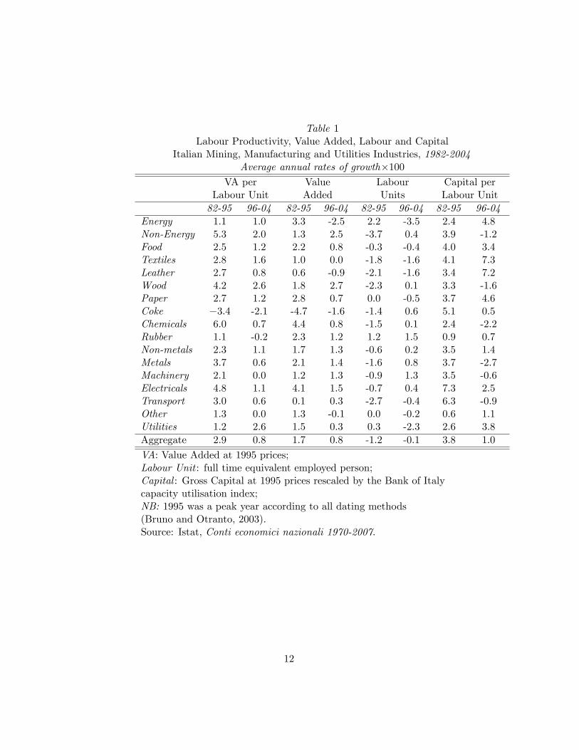
Table 1Labour Productivity, Value Added, Labour and Capital

Italian Mining, Manufacturing and Utilities Industries, 1982-2004Average annual rates of growth�100

VA perLabour Unit

ValueAdded

LabourUnits

Capital perLabour Unit

82-95 96-04 82-95 96-04 82-95 96-04 82-95 96-04

Energy 1:1 1.0 3.3 -2.5 2.2 -3.5 2.4 4.8Non-Energy 5:3 2.0 1.3 2.5 -3.7 0.4 3.9 -1.2Food 2:5 1.2 2.2 0.8 -0.3 -0.4 4.0 3.4Textiles 2:8 1.6 1.0 0.0 -1.8 -1.6 4.1 7.3Leather 2:7 0.8 0.6 -0.9 -2.1 -1.6 3.4 7.2Wood 4:2 2.6 1.8 2.7 -2.3 0.1 3.3 -1.6Paper 2:7 1.2 2.8 0.7 0.0 -0.5 3.7 4.6Coke �3:4 -2.1 -4.7 -1.6 -1.4 0.6 5.1 0.5Chemicals 6:0 0.7 4.4 0.8 -1.5 0.1 2.4 -2.2Rubber 1:1 -0.2 2.3 1.2 1.2 1.5 0.9 0.7Non-metals 2:3 1.1 1.7 1.3 -0.6 0.2 3.5 1.4Metals 3:7 0.6 2.1 1.4 -1.6 0.8 3.7 -2.7Machinery 2:1 0.0 1.2 1.3 -0.9 1.3 3.5 -0.6Electricals 4:8 1.1 4.1 1.5 -0.7 0.4 7.3 2.5Transport 3:0 0.6 0.1 0.3 -2.7 -0.4 6.3 -0.9Other 1:3 0.0 1.3 -0.1 0.0 -0.2 0.6 1.1Utilities 1:2 2.6 1.5 0.3 0.3 -2.3 2.6 3.8

Aggregate 2:9 0.8 1.7 0.8 -1.2 -0.1 3.8 1.0

VA: Value Added at 1995 prices;Labour Unit : full time equivalent employed person;Capital : Gross Capital at 1995 prices rescaled by the Bank of Italycapacity utilisation index;NB: 1995 was a peak year according to all dating methods(Bruno and Otranto, 2003).Source: Istat, Conti economici nazionali 1970-2007.

12

Table 2Labour Productivity, Labour and Capital/Labour ratio

Panel Unit Root Tests 1981-2004

VA perLabour Unit

LabourUnits

Capital perLabour Unit

CIPSC �1:71 �1:23 �1:51CIPST �1:63 �1:46 �1:56

CIPS : truncated mean of the individual ADF statisticsaugmented with cross-section means; panel: all industriesof the Mining, Manufacturing and Utilities Sectionsexcept Energy Mining and Coke (N = 15).CIPSC : CIPS statistic with constant;CIPST : CIPS statistic with constant and trend.Critical values (T = 20; N = 15):constant : 5%� 2:26; 10%� 2:14;trend: 5%� 2:78; 10%� 2:67.

3 Modelling Labour Productivity

Although the economic analysis of productivity is well-known (to say theleast) we shall brie�y review some basic concepts in order to establish nota-tion.

We are interested in Labour Productivity trends in a panel of N indus-tries over T time periods. Since data on intermediate inputs are not availablewe measure production by Value Added (Y ), rather than the theoreticallypreferable Gross Output. Denoting by Fi a generic production function forindustry i, by L and K; as usual, respectively labour inputs and capital; byP a time-dependent factor capturing Hicks-neutral technical progress; we areessentially interested in estimating the function Yit = PitFi(Lit;Kit): Sincecapital-labour substitution is a central issue a Cobb-Douglas speci�cation,which assumes elasticity of substitution equal to 1, is out of question. Someexperimentation with the Translog, the most general production function,delivered unsatisfactory results (coe¢cient estimates often non signi�cant,with many implausible values) because of near perfect multicollinearity inalmost all industries. This problem is indeed often reported in the literature(see, e.g., Harrigan, 1999, Hsiao, Shen and Fujiki, 2002). The only viableoption thus seems to be the Kmenta (1967) linearisation of the CES around

13

the point implying capital-labour elasticity of substitution equal to 1:

yit = �i + pit + �0ilit + �1ikit + �2i(kit � lit)2 + "it (1)

where lower-case letters indicate logs and �i is a scale parameter. Sub-tracting log labour inputs from both sides of (1) and rearranging we �nallyobtain an equation for log labour productivity (�) under CES technologywith unconstrained returns to scale:

�it = �i + pit + (�0i + �1i � 1)lit + �1i(kit � lit) + �2i(kit � lit)2 + "it: (2)

The CES with constant returns to scale and the Cobb-Douglas may bereadily obtained from (2) excluding respectively the labour and squaredcapital-labour ratio terms.

Before examining in detail the issue of technical progress two points mustbe discussed. First, although (2) allows for an elasticity of substitution dif-ferent from 1, the linearisation is valid only for small deviations from thisvalue. Thus, although estimates of the elasticity of substitution very distantfrom 1 have been reported in the literature (for instance, the coe¢cientsestimated by Du¤y and Papageorgiu, 2000, implie an elasticity of substitu-tion close to 2.5) the results obtained must be interpreted with great care.Estimated elasticities close to 1 should be regarded as inconclusive, ratherthan supporting the Cobb-Douglas hypothesis.

Second, since, as we will see below, capital per labour unit is non-stationary the presence of its square brings us into the domain of asymptoticsfor non-linear transformations of integrated series. Fortunately, things turnout to be very simple, as Park and Phillips (1999) showed that with functionssuch as the square power of interest here we may expect the OLS estima-tor to be consistent and mixed normal as in the usual linear cointegratingregression.

Let us now move to technical progress, represented in (2) by the termpit which can be described as a �technology shift parameter� (Mahony andVecchi, 2003) or a �total factor productivity [TFP] index� (Harrigan, 1999),and which is obviously unobserved. The elusive nature of technical progressis tackled in the production function literature in various, generally unsat-isfactory, ways. In time series studies pit is modelled assuming a priori aconvenient functional form (generally, a linear trend). In panel studies TFPdynamics is typically ignored, and the focus centred on measuring e¢ciencydi¤erentials assumed to be constant over time, hence empirically measuredby the �xed e¤ects in panel regressions with homogenous elasticities (e.g.,

14

Islam, 1995, and for the Italian case, Marrocu, Paci and Pala, 2001). Fi-nally, a mixture of the two approaches is found in panel studies includinglinear time trends with coe¢cients heterogenous across units, as Harrigan(1999). Hence, with scant exceptions such as Kee (2004), the TFP trend isnever estimated: either assumed or ignored.

We shall now argue that these approaches are uneccessarily restrictive;exploiting the panel structure of the data we can estimate the TFP trendunder much looser assumptions. More speci�cally, similarly to Kee (2004),assume the log TFP index, pit; to admit a decomposition

pit = �t + it (3)

where:

(i) �t is a, possibly non-stationary, common factor capturing the economy-wide trend in technical progress;

(ii) it = i + 0it is a stationary industry (log) shift factor capturingthe di¤erent rates of adoption of the general technical progress in thevarious industries. Fast growing, high technology industries will havemean (log) shift factor i > 0; while for mature industries i < 0.Idyosincratic departures from the mean shift factor may be caused bythe mean zero, homoskedastic random errors 0it:

In other terms, we are assuming that there exists a common trend intechnical progress (�t), which is transmitted to each industry according to itsown rate of adoption, captured by a log-additive shift factor ( it), equivalentto a varying slope in natural units. Hence, technology shocks coming fromthe the common trend have larger impacts on some industries (the hightechnology ones, where there is much scope for exploiting new products orprocesses) than in others (the mature industries, where the opposite holds).This approach is consistent with the important recent developments of theliterature on non-stationary panels based on the assumption of a commonfactor to handle dependence (see, e.g., Pesaran, 2006, and Gengenback,Palm, Urbain, 2006).

Substituting (3) into (2) we obtain:

�it = �0i + �t + (�0i + �1i � 1)lit + �1i(kit � lit) + �2i(kit � lit)2 + "0it: (4)

where �0i = �i + i and "0

it = "it + 0

it:

In order to estimate model (4) we need to �nd an empirical counterpartfor the unobserved technical progress variable component, �t: As mentioned

15

above, exploiting the panel structure of the data this turns out to be arelatively simple task. De�ne a set of time dummies D� = 1 if t = � ; 0 else,t = 2; : : : ; T (one of the time periods must be excluded to avoid singularity);an heterogenous panel long-run model of labour productivity based on (4)including common time dummies is given by:

�it = �i + 0ilit + 1i(kit � lit) + 2i(kit � lit)2 + 'tDt + eit (5)

t = 1; 2; : : : ; T , i = 1; 2; : : : ; N

Note that the panel is highly heterogeneous: �xed e¤ects are included, andfactor elasticities allowed to vary across industries (contrary to typical panelapplications, as e.g., the papers quoted above by Islam, 1995, and Marrocuet al., 2001, where some homogeneity is always assumed). Only the coe¢-cients of the time dummies, ' = ['2'3 : : : 'T ]; are common to all industries.Hence, they measure the shifts in labour productivity which in every periodcannot be explained by changes in Capital/Labour ratio and, when 0i 6= 0so that returns to scale are di¤erent from one, changes in scale of produc-tion, thus corresponding precisely to the term �t in model (4). It is worthremarking that, as mentioned in the Introduction, following this approachto obtain a set of TFP estimates we only need data on inputs and output�ows. Information on the rental price of capital, always less reliable thanthese basic �ow data and often not even available, is not required.

Since all variables included in (5) should generally be expected, and in-deed in our case are, non-stationary, its estimation involves two distincttasks: (i) testing for cointegration to ensure the relationship is not spurious;(ii) estimating its parameters. The �rst task requires a panel cointegrationtest robust to both short and long-run dependence across units (previousstudies, such as Marrocu, et al., 2001, ignored this crucial point and usedtests valid only for independent units) and, given that in our 1981-2004panel of the Italian Manufacturing Industries we have T = 24 and N = 15;able to deliver good small sample performances. While the former require-ment is satisfyied by various tests, including asymptotic procedures basedon the common factor approach (e.g., Gengenback, Palm, Urbain, 2006),the latter singles out as the only viable option the bootstrap procedure forthe mean and median of the individual cointegration ADF statistics pro-posed by Fachin (2007). The second task, estimation, might in principle becarried out using the OLS estimates computed for the cointegration tests.However, OLS estimates in I(1) regressions are biased, ine¢cient, and donot converge even asymptotically to a known distribution, so that the pointestimates maybe of poor quality and no inference is possible. This suggests

16

that the second task should be carried out using a more suitable method ableto account for the non-stationary nature of the data. In principle Fully Mod-i�ed SUR system estimation (Moon, 1999) may appear the ideal solution.However, in our dataset this is practically unfeasible, as the time dimensiononly marginally larger than the cross-section dimension makes estimationof the long-run covariance matrix in practice an unfeasible task (Pedroni,1997, Di Iorio and Fachin, 2008). We shall then apply the following iterativetwo-steps procedure:

Step A Estimate the panel regression (5) by OLS, and:

A1. compute the panel cointegration tests by Fachin (2007); details aregiven in the Appendix;

A2. recover the TFP trend as the vector of the coe¢cients of the timedummies Dt (b' ):

A3. compute the deviations of labour productivity from the TFP trend:e�it = �it � b't;

Step B estimate the equations e�it = �i + 0ilit + 1i(kit � lit) + 2i(kit � lit)2 + eit

separately for each industry by FM-OLS.

If Step B suggests that some coe¢cients should be constrained to zeroStep A is repeated on the constrained speci�cation, until a satisfactory spec-i�cation is reached.

Given the small sample size, hence the low power of the signi�cance tests,we chose to delete the labour variable when appropriate (thus moving to aspeci�cation implying constant returns to scale), while the capital variableshave been excluded only when the coe¢cients turned out to be negative,clear sign of a spurious relationship. Variables with non-signi�cant coef-�cients have been retained in a few cases when this delivered overall themost meaningful equations; given the small time sample and the collinearityproblems of the dataset at hand this is not unexpected.

The �nal test statistics and estimates are reported in Table 4, with plotsin Fig. 5. To account for possible changes in the industry shift coe¢cientswe split the constant at 1995, a cyclical turning point when TFP growthaccording to growth accounting estimates slowed down signi�cantly (Istat,2007). Since no meaningful estimates could be obtained for the residualsector "Other industries" this has been dropped from the panel. Given itscomposition (it includes activites as diverse as, e.g, production of toys and

17

musical instruments and recycling) this is not surprising. Taking into ac-count that with the available sample size the power of the test must to beexpected to be rather low (Fachin, 2007) the hypothesis of no panel cointe-gration for the restricted speci�cation, with p-values below 1% in mean andjust above 5% in median, can be safely considered as rejected. The coe¢cientof labour units is most cases signi�cant, suggesting non-constant returns toscale, mostly decreasing. The quadratic term is generally signi�cant, but theestimates of the elasticity of substitution between labour and capital are fartoo volatile to be credible. Given that this parameter is a highly non-linearfunction of the coe¢cients of the production function this �nding is not toosurprising; it is also consistent with Balistreri, McDaniel and Wong (2003),who report for 28 US industries over the period 1947-1998 point estimatesclose to 1 but very wide con�dence intervals. A possible explanation may beaggregation bias, with factor reallocation within industries causing the same(di¤erent) aggregate combinations of inputs producing di¤erent (the same)levels of aggregate output, and ultimately uncertainty in the estimation ofthe elasticities.

18

Table 3Modelling Labour Productivity, 1981-2004Mining, Manufacturing and Utilities

Panel Cointegration Bootstrap p� values� 100Tests simple FDB1 FDB2

Mean t �2:73 1:0 0:4 �0:5

Median t �3:70 11:2 8:7 6:5

FM-OLS estimatesDeviations from estimated TFP trend

Industries 0 1 2 �0 �1 ES(K;L) Z�Non-Energy 0:35

(1:60)1:99(3:57)

0:35(1:80)

3:94(7:28)

� 0:19(11:11)

�0:30 �23:93

Food 0:72(2:51)

1:82(2:55)

0:49(2:54)

0:57(0:41)

� �0:28 �17:80

Textiles � 5:37(10:77)

1:04(10:27)

9:72(16:27)

0:08(4:33)

�24:74 �10:86

Leather 0:66(4:33)

6:23(5:12)

0:95(4:82)

9:31(6:40)

0:07(4:03)

�0:08 �11:40

Wood � 1:86(1:86)

0:38(1:58)

5:10(5:01)

�0:08(3:87)

1:62 �13:77

Paper �0:13(0:67)

0:17(6:04)

� 4:48(4:29)

0:07(3:51)

1 �14:27

Chemicals 0:98(4:63)

1:43(11:60)

� �0:21(0:20)

0:06(3:69)

1 �13:06

Rubber �0:70(0:02)

36:52(5:35)

12:09(5:42)

34:74(6:90)

�0:09(4:72)

0:06 �13:87

Non-metals 0:15(4:60)

0:83(6:01)

0:15(4:32)

3:58(18:16)

�0:01(2:00)

�0:44 �19:64

Metals � 3:03(7:60)

0:69(6:78)

6:46(16:82)

� 3:27 �4:64

Machinery � 0:64(0:78)

0:16(0:80)

4:09(5:13)

0:02(1:03)

1:19 �16:11

Electricals 0:30(1:83)

0:29(14:79)

� 2:23(2:32)

� 1 �15:65

Transport 0:78(3:18)

0:17(1:74)

� �0:77(0:61)

� 1 �7:90

Utilities �0:06(1:85)

1:13(12:07)

4:34(135:10)

0:07(2:27)

� �7:67 �12:86

Model : e�it = �0i + �1i� t + 0lit + 1(kit � lit) + 2(kit � lit)2 + "it

e�it = �it � b't; b't : see equation (5);� t = 1 if t < 1995, 0 else;ES(K,L): Labour-Capital Elasticity of substitution;Z� 10% critical point :�23:54Bootstrap: 5000 redrawings, block size 4.FDB1; FDB2 : Davidson and McKinnon (2000) Fast Double BootstrapType 1 and Type 2.

19

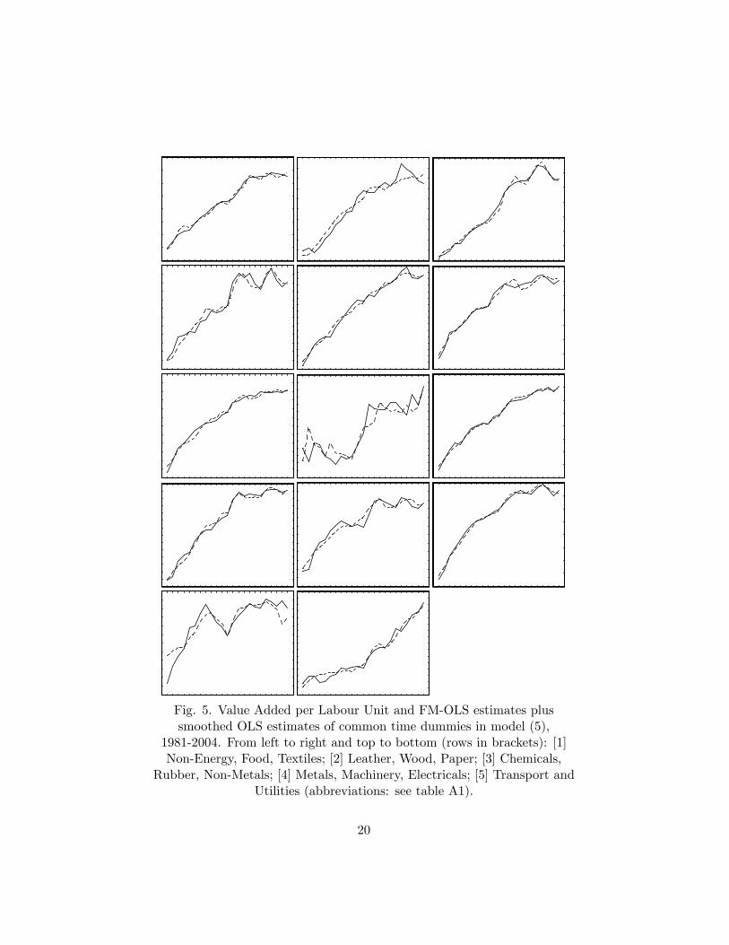
Fig. 5. Value Added per Labour Unit and FM-OLS estimates plussmoothed OLS estimates of common time dummies in model (5),

1981-2004. From left to right and top to bottom (rows in brackets): [1]Non-Energy, Food, Textiles; [2] Leather, Wood, Paper; [3] Chemicals,

Rubber, Non-Metals; [4] Metals, Machinery, Electricals; [5] Transport andUtilities (abbreviations: see table A1).

20

Let us now examine TFP estimates. In Fig. 6 we plotted the �rstdi¤erences of the coe¢cients along with those obtained following the growthaccounting approach by Istat (2007). As w can seen, the results are striking.Following a method entirely di¤erent we end up drawing essentially similarpictures: a falling trend reversed only temporarily in the early-�90�s. Thisevidence thus appears to robust to the estimation method adopted.

Fig. 6. Alternative estimates of TFP growth rates, 1982-2004: Panelestimates: �rst di¤erences of coe¢cients of time dummies in model (5)estimated on all Manufacturing industries except "Energy Mining", "Oil"

and "Other Industries". Istat: growth accounting estimates, entireManufacturing industry (Istat, 2007).

The next natural step is trying to shed some light on the determinants ofTFP growth. To this end we estimated a simple model with a set of explana-tory variables including the standard deviations across the I industries of

the log di¤erences of labour, ��lt , and capital per labour unit, ��(k�l)t (i:e:,

��xt = [I�1PIj=1(�xjt��xt)

2]1

2 ; x = l; (k� l)), so to capture factor reallo-cation across industries, R&D expenditure growth (�rd), a human capital

21

index (h), and �nally,to capture factor reallocation across capital types, thestandard deviations across types (machinery, buildings, computers, commu-nication equipment, software, furniture, transportation equipment) of �xedcapital growth. To avoid endogeneity all variables have been included withone lag.

The results, reported in Table 4, appear interesting. Factor reallocation,as measured by growth variability across industries, is strongly signi�cant,while there seems to be a weaker but not totally negligible e¤ect of shiftsin capital composition. R&D expenditure is not signi�cant, which is notsurprising in view of the results reported by Atella and Quintieri (2001).Finally, the failure to detect a signi�cant in�uence of changes in humancapital may be at least partially due to measurement problems.

Table 4Determinants of TFP growth, 1982-2004

��lt�1 ��(k�l)t�1 �h1t�1 �h2t�1 �rdt �Kt�1 const

1:71(2:65)

7:62(3:59)

0:03(1:08)

0:007(0:73)

0:09(0:97)

0:04(1:38)

�0:21(�3:95)

se = 0:02;LM(p) = 0:57 (0:46)

Dependent variable: �rst di¤erence of the coe¢cients ' of the common timedummies Dt in model (5);��x = variance of growth rates of factor x across branches;�hj : log di¤erence of human capital index, j = 1 : t < 1992(break in the series), j = 2 : t > 1992;�rd : log di¤erence of R&D expenditure;�K : variance of growth rates across capital types;t-statistics in brackets underneath the estimates;se : standard error of residuals;LM : test for no �rst order autocorrelation (p-value in brackets).

4 Conclusions

In this paper we reached conclusions arguably of some interest both fromthe methodological and the empirical point of view. First of all, building onrecent developments in the analysis of non-stationary, dependent panels, we

22

developed a method for obtaining estimates of TFP trends (i) free from therestrictive assumptions needed by traditional growth accounting and (ii)requiring only data on inputs and output �ows, and able to deliver esti-mates of long-run TFP trends. It is thus arguably more general than boththe growth accounting and Kee�s (2004) structural model-based approaches.Applying it to the Italian manufacturing industries we obtain results con-�rming the conclusion already reached by growth accounting, i.e. that thedecline in Italian labour productivity in the past decade has been mostlydue to a widespread fall in TFP growth. A simple regression suggests thatthe most obvious culprits, namely the completion of a factor reallocationprocess among industries and capital types, did actually play an importantrole in this decline.

5 References

Atella, V. and B. Quintieri (2001) "Do R&D expenditures really matterfor TFP?" Applied Economics, 33, 1385-1389.

Balistreri, E.J., McDaniel, C.A., Wong, E.V. (2003) �An estimation ofUS industry-level capital-labor substitution elasticities: support forCobbDouglas� North American Journal of Economics and Finance,vol. 14, 343-356.

Barba Navaretti, G., R. Faini and A. Tucci (2005) �Competitività ed at-tività internazionali delle imprese Italiane�

Bassanetti, A., M. Iommi, C. Jona-Lasinio and F. Zollino (2004) �Lacrescita dell�economia italiana negli anni novanta tra ritardo tecno-logico e rallentamento della produttività� Temi di discussione n. 539,Banca d�Italia.

Bernanke, B.S. (2005) � Remarks� C. Peter McColough Roundtable Serieson International Economics, Council on Foreign Relations Universityof Arkansas at Little Rock Business Forum

Brandolini, A., and P. Cipollone (2001) �Multifactor Productivity andLabour Quality in Italy, 1981-2000� Banca d�Italia, Temi di discus-sione n. 422

Bruno, G. and E. Otranto (2003) �Dating the Italian Business Cycle: AComparison of Procedures� Working Paper, University of Sassari.

23

Centraal Planbureau �Recent trends in Dutch labor productivity: the roleof changes in the composition of employment� Working Paper n. 98CPB Netherlands Bureau for Economic Policy Analysis, The Hague(NL)

Conference Board (2007) �Global Productivity Trends� http://www.conference-board.org/economics/

Davidson R., and J.G. MacKinnon (2000) "Improving the Reliability ofBootstrap Tests" Queen�s University Institute for Economic ResearchDiscussion Paper No. 995.

Daveri, F. (2004) �Why is there a productivity problem in Europe?� CEPSWorking Documents n. 205.

Daveri, F. and C. Jona-Lasinio (2005) �Italys Decline: getting the factsright� IGIER Università Bocconi, Working Paper n. 301.

Denison, E.F. (1967) Why Growth Rates Di¤er: Postwar Experience inNine Western Countries The Brookings Institution, Washington (USA).

Di Iorio, F. and S. Fachin (2008) "A Note on the Estimation of Long-Run Relationships in Dependent Cointegrated Panels" Working Paper,University of Rome "La Sapienza".

Dolman, B., L. Lu and J. Rahman (2005) �Understanding productivitytrends� Australian Treasury.

Du¤y, J. and C. Papageorgiu (2000) �A Cross-Country Empirical Inves-tigation of the Aggregate Production Function Speci�cation� Journalof Economic Growth, 5, 87-120.

Fachin, S. (2007) �Long-Run Trends in Internal Migrations in Italy: aStudy in Panel Cointegration with Dependent Units� Journal of Ap-plied Econometrics, 22, 401-428.

Gengenback, C., F.C. Palm, J.P. Urbain (2006) �Cointegration Testingin Panels with Common Factors� Oxford Bulletin of Economics andStatistics, 768, 684-719.

Harrigan, J. (1999) �Estimation of cross-country di¤erences in industryproduction functions� Journal of International Economics, 47, 267-293.

24

Hsiao, C., Y. Shen and H. Fujiki (2002) �Aggregate vs Disaggregate DataAnalysis - A Paradox in the Estimation of Money Demand Functionof Japan Under the Low Interest Rate Policy� Working Paper, UCLA(USA).

Im, K., M.H. Pesaran and Y. Shin (2003) �Testing for Unit Roots in Het-erogeneous Panels� Journal of Econometrics, 115, 53-74.

Islam, N. (1995) �Growth Empirics: a Panel Data Approach� QuarterlyJournal of Economics, 110, 1127-1170.

Istat (2007) "Misure di produttività - Anni 1980-2006" Statistiche in breve,5 Ottobre 2007.

Kee, H. L. (2004) �Estimating Productivity When Primal and Dual TFPAccounting Fail: An Illustration Using Singapores Industries� Topicsin Economic Analysis & Policy, vol. 4, article 26.

Kmenta, J. (1967) �On the Estimation of the C.E.S. Production Function�International Economic Review, 2, 180-89.

Mahony, M. and M. Vecchi (2003) �Is there an ICT impact on TFP? Aheterogeneous dynamic panel approach� Working Paper, NIESR.

Marrocu, E., R. Paci and R. Pala (2001) �Estimation of total factor produc-tivity for regions and sectors in Italy. A panel cointegration approach�RISEC, 48, 533-558.

Matthews, R.C.O., C.H. Feinstein and J. C. Odling-Smee (1982) BritishEconomic Growth 1856-1973 Oxford University Press, Oxford (UK).

Moon, H.R. (1999) "A note on fully-modi�ed estimation of seemingly unre-lated regressions models with integrated regressors" Economics Letters65, 25-31.

Paparoditis, E. and D.N. Politis (2001) �The Continuous-Path Block Boot-strap� In Asymptotics in Statistics and Probability. Papers in honorof George Roussas. Madan Puri (ed.). VSP Publications: Zeist (NL).

Park, J. Y., Phillips, P.C.B. (1999) �Asymptotics for Non-linear Transfor-mations of Integrated series� Econometric Theory, 15, 269-298.

Pedroni, P. (1997) �Cross Sectional Dependence in Cointegration Tests ofPurchasing Power Parity in Panels� Working Paper, Indiana Univer-sity.

25

Pesaran, M.H. (2006) �A Simple Panel Unit Root Test in the Presence ofCross Section Dependence�. DAE Working Paper No. 0346, Cam-bridge University.

Politis, D.N., Romano, J.P. (1994) The stationary bootstrap, Journal ofthe American Statistical Association, 89, 1303-1313.

Silverman, B.W. (1986) Density Estimation for Statistics and Data Analy-sis, Chapman & Hall, London.

Stiroh, K.J. (2002) �Information Technology and the U.S. ProductivityRevival: What Do the Industry Data Say?� The American EconomicReview, 92, 1559-1576.

6 Appendix

6.1 A Bootstrap Panel Cointegration Test

A panel cointegration test suitable for our dataset needs to be robust toboth short-run and long-run dependence across units, so that the asymptotictests usually applied in the literature are not suitable. Fachin (2005) putforth a bootstrap test satisfying both requirements. The test is based on theContinuous-Path Block Bootstrap (CBB), which is applied independently tothe cross-sections of time-series of the X�s, fX1X2 : : : XNg

Tt=1 and the Y

0s

fY1Y2 : : : YNgTt=1. Developed by Paparoditis and Politis (2001), the CBB is a

block resampling method designed to construct non-stationary pseudodata.The pseudo-series is obtained in two steps: �rst, a block bootstrap series isconstructed integrating within each block the resampled �rst di¤erences ofa series known to be non-stationary; second, the end points of the blocks arechained so to eliminate jumps between blocks (this implies that the pseudo-series are shorter than the original series, as one observation must be deletedwhen chaining two blocks). As the resampling is applied to the entire cross-section the pseudo-series will clearly preserve the cross-correlation structureof the non-stationary individual time series. On the other hand, the blocksare chosen independently for the X 0s and the Y 0s, so that the two pseudo-series are independent by design. Denoting by G a group mean statistic theproposed bootstrap procedure includes �ve simple steps:

1. compute the Group statistic bG for the data set under study,

fX1X2 : : : XN ; Y1Y2 : : : YNgTt=1;

26

2. construct separately by CBB two sets of N pseudo-series,

fX�

1X�

2 : : : X�

NgT �

t=1 and fY�

1 Y�

2 : : : Y�

NgT �

t=1;

3. compute the Group statistics G� for the pseudo-data set,

fX�

1X�

2 : : : X�

N ; Y�

1 Y�

2 : : : Y�

NgT �

t=1;

4. repeat steps (2) and (3) a large number (say, B) of times;

5. compute the boostrap signi�cance level; assuming that the rejectionregion is the left tail of the distribution, p� = prop(G� < bG).

6.2 Data

6.2.1 De�nitions and Sources

Labour Productivity Value Added per Labour Unit.

Value Added At 1995 prices. Istat, Conti economici nazionali 1970-2007.

Labour Units Istat�s implementation of the ESA95 concept of full timeequivalent employee. Istat, Conti economici nazionali 1970-2007.

Capital Gross Capital stock at 1995 prices. Istat, Conti economici nazionali1970-2007.

Capacity Utilisation Bank of Italy Utilisation Index. Because of the lowerdetail of this index with respect to the data on capital stock in the dis-aggregate analysis the following approximations have been introduced:(i) the index for �Leather and Textiles� has been used for both theTextile and the Leather industries; (ii) the manufacturing index hasbeen used for the both the Non metals; (iii) the economy-wide indexhas been used for the Utilities.

Research and Development expenditure: share of GDP. OECD, Main Sci-ence and Technology Indicators.

Human Capital Index : Average education of workforce weighted with av-erage net wages, index 1977=100. Brandolini and Cipollone (2001).

27

6.2.2 Industry Classi�cation

The NACE Rev. 1.1 Classi�cation:Sections C, D and E and their Subsections

Abbreviation GDP Share Share

Section C Mining and Quarrying Mining 0.5 1.9

Mining and quarrying of energy Energy 0.3 1.2producing materialsMining and quarrying, except of Non-Energy 0.2 0.7energy producing materials

Section D Manufacturing Manufacturing 20.3 90.3

Food products, beverages and tobacco Food 2.0 8.4Textiles and textile products Textiles 2.1 8.9Leather and leather products Leather 0.7 2.7Wood and wood products Wood 0.5 2.2Pulp, paper and paper products; Paper 1.2 5.1publishing and printingCoke, re�ned petroleum products Coke 0.4 1.6and nuclear fuelChemicals, chemical products and Chemicals 1.5 6.2man-made �bresRubber and plastic products Rubber 0.8 3.4Other non-metallic mineral products Non-metals 1.2 4.8Basic metals and fabricated Metals 3.0 12.3metal productsMachinery and equipment n.e.c. Mach 2.4 9.9Electrical and optical equipment Electricals 1.9 8.0Transport equipment Transport 1.2 4.9Manufacturing n.e.c. Other 1.0 4.2

Section E Electricity, Gas and Utilities 1.9 7.7Water Supply

GDP Share: average 1981-2004 GDP share�100.Share: average 1981-2004 share�100 of the total value added ofSections C, D and E.Source: Istat, Conti economici nazionali 1970-2007.

28