The Cyclicality of the Opportunity Cost of Employment∗

Gabriel Chodorow-ReichHarvard University and NBER

Loukas KarabarbounisChicago Booth, FRB of Minneapolis, and NBER

August 2015

Abstract

The flow opportunity cost of moving from unemployment to employment consists

of foregone public benefits and the foregone value of non-working time in units of con-

sumption. We construct a time series of the opportunity cost of employment using

detailed microdata and administrative or national accounts data to estimate benefit

levels, eligibility and take-up of benefits, consumption by labor force status, hours

per worker, taxes, and preference parameters. Our estimated opportunity cost is pro-

cyclical and volatile over the business cycle. The estimated cyclicality implies far

less unemployment volatility in many leading models of the labor market than that

observed in the data, irrespective of the level of the opportunity cost.

JEL-Codes: E24, E32, J64.

Keywords: Opportunity Cost of Employment, Unemployment Fluctuations.

∗Chodorow-Reich: Harvard University Department of Economics, Littauer Center, Cambridge, MA 02138 (e-

mail: chodorowreich@fas.harvard.edu); Karabarbounis: Federal Reserve Bank of Minneapolis, 90 Hennepin Avenue,

Minneapolis, MN 55401 (email: loukas.karabarbounis@chicagobooth.edu). We are especially grateful to Bob Hall

for many insightful discussions and for his generous comments at various stages of this project. This paper also

benefited from comments and conversations with Mark Bils, Steve Davis, Dan Feenberg, Peter Ganong, Erik Hurst,

Greg Kaplan, Larry Katz, Pat Kehoe, Guido Lorenzoni, Iourii Manovskii, Kurt Mitman, Giuseppe Moscarini, Casey

Mulligan, Nicolas Petrosky-Nadeau, Richard Rogerson, Rob Shimer, Harald Uhlig, Gianluca Violante, anonymous

referees, and numerous seminar participants. Much of this paper was written while Gabriel Chodorow-Reich was

visiting the Julis-Rabinowitz Center at Princeton University. Loukas Karabarbounis thanks Chicago Booth for

summer financial support. The Appendix and dataset that accompany this paper are available at the authors’

webpages. The views expressed herein are those of the authors and not necessarily those of the Federal Reserve

Bank of Minneapolis or the Federal Reserve System.

1 Introduction

Understanding the causes of labor market fluctuations ranks among the most important and

difficult issues in economics. In recent decades, economists have turned attention to models of

equilibrium unemployment. These models feature optimization decisions by workers and firms

along with frictions which prevent all workers from supplying their desired amount of labor.

The flow value of the opportunity cost of employment, which we denote by z, plays a crucial

role in many such models. The importance of this variable has generated debate about its

level, but the literature has almost uniformly adopted the assumption that the opportunity cost

is constant over the business cycle. Fluctuations in the opportunity cost correspond loosely

to shifts in desired labor supply and, therefore, can affect the volatility of unemployment and

wages. While this insight goes back at least as far as Pissarides (1985), to date the cyclical

properties of the opportunity cost in the data remain unknown.

The main contribution of this paper is to develop and implement an empirical framework

to measure z in the data.1 We find that, irrespective of its level, z is procyclical and volatile

over the business cycle. The cyclicality of z poses a significant challenge to models that rely on

a constant z to solve the unemployment volatility puzzle highlighted by Shimer (2005). This is

because a procyclical z undoes the endogenous wage rigidity generated by these models.

We begin in Section 2 by deriving an expression for the opportunity cost z. We start

our analysis within a framework that borrows elements from the search and matching model

developed in Mortensen and Pissarides (1994) (hereafter MP model). We show, however, that

the same measure of z also arises naturally in many other environments. For example, the

same expression for z plays an important role in models that allow for ex-ante heterogeneity

across workers, models that use alternative wage bargaining protocols, and models with directed

instead of random search. In this wide class of models, fluctuations in equilibrium unemployment

depend on the behavior of z relative to the behavior of the after-tax marginal product of

employment (which we denote by pτ ).

1Our approach complements recent research that uses surveys to ask respondents directly about their reservationwage (Hall and Mueller, 2013; Krueger and Mueller, 2013). Relative to survey estimates, our approach allows usto construct a long time series for z, which is crucial for studying cyclical patterns.

1

We write the opportunity cost of employment as the sum of two terms, z = b + ξ. The

first term, which we denote by b, is the value of public benefits that unemployed forgo upon

employment. Our expression for b departs from the literature in three significant ways. First, we

argue that b should depend on effective rather than statutory benefit rates. Second, we consider

both unemployment insurance (UI) benefits, which are directly related to unemployment status,

and non-UI benefits such as supplemental nutritional assistance (SNAP), welfare assistance

(AFDC/TANF), and health care (Medicaid). The latter belong in the opportunity cost to

the extent that receipt of these benefits changes with unemployment status. Third, we take

into account UI benefits expiration, incorporate taxes, and model and measure the utility costs

associated with taking up UI benefits (for instance, job search costs and other filing and time

costs). These utility costs allow the model to match the fact that roughly one-third of eligible

unemployed do not actually take up UI benefits.

In Section 3 we measure b over the period 1961(1) to 2012(4). For the measurement of b

we require time series of UI and non-UI benefits per unemployed. Combining household and

individual-level data from the Current Population Survey (CPS) and the Survey of Income and

Program Participation (SIPP) with program administrative data, we estimate the value of UI,

SNAP, AFDC/TANF, and Medicaid benefits that belong in b. We further incorporate into

our measurement of b the time series of UI eligibility, take-up rates, and number of recipients.

Finally, we use IRS Public Use Files to estimate tax rates on UI benefits.

Our estimated b is countercyclical, rising around every recession since 1961. However, be-

cause we incorporate effective rather than statutory rates and because we account for costs

associated with UI take-up and for the expiration of UI benefits, the level of b is much smaller

than what the literature has traditionally calibrated. We find that b is only 6 percent of the

sample average of the after-tax marginal product of employment pτ .

The second term of the opportunity cost of employment z = b+ξ, which we denote by ξ, is the

foregone value of non-working time expressed in units of consumption. With concave preferences

over consumption and an explicit value of non-working time, this component resembles the

marginal rate of substitution between non-working time and consumption in the real business

2

cycle (RBC) model, with the difference being that the value of non-working time is calculated

along the extensive margin. In the RBC model, an intraperiod first-order condition equates

the marginal rate of substitution between non-working time and consumption to the after-tax

marginal product of labor. While the search and matching literature has appealed to this

equality to motivate setting the level of z close to that of the marginal product, the same logic

suggests that the ξ component of z would move cyclically with the marginal product just as in

the RBC model.

We measure the ξ component of the opportunity cost in Section 4. For the measurement of

ξ we require estimates of preference parameters and time series of consumption expenditures by

labor force status, hours per worker, and labor income and consumption taxes. The consumption

of the employed and unemployed do not have direct counterparts in existing data sources. We

generate time series of consumptions using estimates of relative consumption by labor force

status from the Consumer Expenditure Survey (CE) and the Panel Study of Income Dynamics

(PSID), population shares by labor force status, and NIPA consumption of non-durables and

services per capita. We measure hours per worker from the CPS. Finally, we use IRS Public

Use Files to estimate tax rates on labor income and NIPA data to measure effective taxes on

consumption.

The measurement of ξ also depends on preference parameters, which we calibrate for various

common utility functions. We discipline preference parameters by requiring that the steady state

of the model be consistent with empirical estimates of hours per worker and the consumption

decline upon unemployment. We present specifications that result in levels of z ranging from

0.47 to 0.96 relative to an after-tax marginal product of employment equal to pτ = 1. We

show how the level of z across these specifications depends on estimates of the total endowment

of utility-enhancing time, the curvature of the utility function, and fixed time or utility costs

associated with working.

We find that the ξ component of the opportunity cost is highly procyclical, irrespective of

its level. This procyclicality reflects the procyclical movements in consumption and hours per

worker. Intuitively, ξ falls in recessions because the household values more the contribution of

3

the employed (through higher wage income) relative to that of the unemployed (through higher

non-working time) in states of the world in which consumption is low and non-working time is

high.

Combining the opportunity cost associated with benefits b with the opportunity cost asso-

ciated with the value of non-working time ξ, Section 5 shows that our time series of z = b+ ξ is

procyclical and volatile. The procyclicality of z reflects the outcome of two opposing forces. In

the absence of ξ, fluctuations in b would imply a countercyclical z. However, because the level

of b is much smaller than the level of ξ, the procyclical ξ component accounts for the majority

of the fluctuations in z.

The elasticity of the cyclical component of z with respect to the cyclical component of

the marginal product of employment p is an informative summary statistic when assessing the

performance of a large class of models. Across specifications, this elasticity exceeds 0.8 and is

typically close to 1. Importantly, z comoves roughly proportionally with p over the business cycle

irrespective of whether the level of z is high or low. The positive and large elasticity appears

robust to a number of alternative modeling choices and data moments, including replacing the

hours per worker series with hours per worker for hourly workers, salaried workers, or an hours

series adjusted for compositional changes over the business cycle, changing the estimated decline

in consumption upon unemployment, using an alternative model of UI take-up, and introducing

fixed time and utility costs associated with working.

In Section 6 we extend our framework to allow for heterogeneity across workers with dif-

ferent educational attainments. While this exercise reveals interesting variation in the level

and composition of z across skill groups, each of the skill-specific z’s is procyclical. The same

economic forces that cause fluctuations in the aggregate z over the business cycle also influence

the skill-specific z’s. Quantitatively, the lowest skill groups exhibit a more elastic z over the

business cycle than the highest skill groups.

Section 7 turns to the implications of our estimated z for models of unemployment fluctu-

ations. We start with models in the MP class. As emphasized in influential work by Shimer

(2005), the standard MP model with wages set according to Nash bargaining fails to account

4

quantitatively for the observed volatility of unemployment. Some of the leading solutions to this

unemployment volatility puzzle rely on a constant z to reduce the procyclicality of wages. The

cyclicality of z dampens unemployment fluctuations in these models. The logic of this result

is quite general and does not depend on the set of primitive shocks driving the business cycle.

Relative to the constant z case, a procyclical z increases the surplus from accepting a job at a

given wage during a recession, which puts downward pressure on equilibrium wages and amelio-

rates the increase in unemployment. The extent to which actual wages vary cyclically remains

an open and important question. Our results suggest that any such wage rigidity cannot be

justified by mechanisms that appeal to aspects of the opportunity cost.

We illustrate the consequences of a procyclical z in the context of two leading proposed solu-

tions to the unemployment volatility puzzle which rely on endogenous wage rigidity. Hagedorn

and Manovskii (2008) show that a large and constant z allows the MP model with Nash wage

bargaining to generate realistic unemployment fluctuations. Intuitively, a level of z close to

the tax-adjusted p makes the total surplus from an employment relationship small on average.

Then even modest increases in p generate large percent increases in the surplus, incentivizing

firms to significantly increase their job creation.2 However, if z and p move proportionally,

then the surplus from a new hire remains relatively stable over the business cycle. As a result,

fluctuations in unemployment are essentially neutral with respect to the level of z.

Hall and Milgrom (2008) generate volatile unemployment fluctuations by replacing the as-

sumption of Nash bargaining over match surplus with an alternating-offer wage setting mech-

anism. With Nash bargaining, the threat point of an unemployed depends on the wage other

jobs would offer in case of bargaining termination. In the alternating-offer bargaining game, the

threat point depends instead mostly on the flow value z if bargaining continues. With constant

z, wages respond weakly to increases in p. Allowing instead z to comove with p as in the data

undoes this endogenous wage rigidity, thereby reducing the volatility of unemployment.

2A number of papers have followed this reasoning to set a relatively high level of z. Hagedorn and Manovskii(2008) use a value of z = 0.955. Examples of papers before Hagedorn and Manovskii (2008) include Mortensenand Pissarides (1999), Mortensen and Pissarides (2001), Hall (2005), and Shimer (2005), which set z at 0.42, 0.51,0.40, and 0.40. Examples of papers after Hagedorn and Manovskii (2008) include Mortensen and Nagypal (2007),Costain and Reiter (2008), Hall and Milgrom (2008), and Bils, Chang, and Kim (2012), which set z at 0.73, 0.745,0.71, and 0.82. See Hornstein, Krusell, and Violante (2005) for a useful summary of this literature.

5

Finally, we show that z plays an important role in equilibrium models outside of the MP

class. We discuss models with directed search and indivisible labor. The same expression for z

enters into the opportunity cost of employment in each of these models and, therefore, plays an

important role in determining unemployment fluctuations.

2 The Opportunity Cost of Employment

We develop an expression for the opportunity cost of employment z within a widely studied

framework that borrows elements from the search and matching model and the real business

cycle model with concave preferences and an explicit value of non-working time. In Section 7.1,

we show that z is a key object for understanding equilibrium unemployment within this standard

MP/RBC model. However, as we discuss below, the same z arises in alternative models that

relax many of the baseline assumptions embedded in the MP/RBC model.

2.1 Household Problem

Time is discrete and the horizon is infinite, t = 0, 1, 2, .... We denote the vector of exogenous

aggregate shocks by Zt. All values are expressed in terms of a numeraire good with a price of

one.

A representative household consists of a continuum of ex-ante identical individuals of measure

one. At the beginning of each period t, there are et employed who produce output and ut = 1−et

unemployed who search for jobs. After production occurs, unemployed find a job in the next

period with probability ft and employed separate and become unemployed with probability st.

Therefore, employment evolves according to the law of motion:

et+1 = (1− st)et + ftut. (1)

Household members treat ft and st as exogenous processes.

The household takes as given employment et at the beginning of each period and the outcome

of any process that determines the wage wt and hours per worker Nt. Household members pool

perfectly their risks and, therefore, the marginal utility of consumption λt is equalized between

the employed and the unemployed. The household owns the economy’s capital stock Kt and

6

rents it to firms in a perfect capital market at a rate rt + δ, where rt denotes the real interest

rate and δ denotes the depreciation rate. Capital Kt accumulates as Kt+1 = (1− δ)Kt + It.

The household chooses consumption of the employed and the unemployed, Cet and Cu

t ,

purchases of investment goods It, and the share of eligible unemployed to take up UI benefits,

ζt, to maximize the expected sum of discounted utility flows of its members:

W h (e0, ω0, K0,Z0) = maxE0

∞∑t=0

βt [etU(Cet , Nt) + (1− et)U(Cu

t , 0)− (1− et)ωtψ(ζt)] , (2)

where U(Cet , Nt) is the flow utility of an employed member, U(Cu

t , 0) is the flow utility of

an unemployed member excluding costs associated with taking up benefits, ωt is the share of

unemployed who are eligible for UI benefits, and ψ(ζt) denotes the household’s costs per eligible

unemployed from taking up UI benefits.

The budget constraint of the household is given by:

(1 + τCt

)(etC

et + (1− et)Cu

t ) + It + Πt = (1− τwt )wtetNt + (1− et)Bt + (rt + δ)Kt, (3)

where Bt denotes after-tax benefits received per unemployed, τCt is the tax rate on consumption,

and τwt is the tax rate on labor income. We denote by Πt the sum of lump sum taxes and the

consumption of individuals out of the labor force net of dividends from ownership of the firms

and other transfers.

2.1.1 Benefits

Benefits Bt received from the government may include after-tax UI benefits as well as other

transfers such as supplemental nutritional assistance, welfare assistance, and health care. Bt

includes only the part of the benefit that an unemployed loses upon moving to employment.3

We split Bt into two components. Non-UI benefits per unemployed, Bn,t, do not involve take-up

costs in our model because the decision and timing of take-up does not generally coincide with

the timing of an unemployment spell. Additionally, non-UI benefits do not generally generate

tax liabilities. UI benefits per unemployed, Bu,t, have a relevant take-up margin and have been

3Benefits that do not depend on labor force status do not affect the value of unemployment relative to employ-ment and are included in the variable Πt.

7

taxed at the federal level since 1979. We write after-tax benefits per unemployed as:

Bt =(1 + τCt

)Bn,t +

(1− τBt

)Bu,t, (4)

where τBt is the tax rate on UI benefits. We multiply non-UI benefits by 1 + τCt because

most of Bn,t, including nutrition assistance and Medicaid, is not subject to consumption taxes.

Therefore, a unit of these benefits is worth 1 + τCt units of (taxable) consumption.

We introduce utility costs of UI take-up into the objective function (2) of the household in

order to account for a take-up rate ζt that in the data is significantly below one, volatile, and

comoves with the benefit level.4 The fact that some of those eligible forgo their UI entitlement

indicates either an informational friction or a take-up cost. The correlation between take-up

and benefits suggests that informational frictions cannot fully explain the low take-up rate. We

interpret these utility costs as foregone time and effort associated with searching for a job and

providing information to the UI agency. We consider an alternative model of take-up without

utility costs in our robustness exercises.

The household’s total cost per eligible unemployed ψt depends on the fraction of those

eligible that take up UI benefits ζt. To see how such a dependence may arise, let ψm(i) denote

the cost of UI take-up by the i ∈ [0, 1] eligible unemployed. We order the heterogeneous costs

as dψm/di > 0. If a fraction ζt of eligible unemployed chooses to take up benefits, then the

total utility cost of taking up benefits per eligible unemployed is:

ψ(ζt) =

∫ ζt

0

ψm (i) di. (5)

The cost function ψ(ζt) is increasing and convex because as ζt increases the marginal recipient

has a higher utility cost. A convex cost function ψ(ζt) guarantees an interior solution for ζt. In

the empirical analysis below, we find evidence of convexity in the data.

Pre-tax benefits per unemployed from UI, Bu,t, are the product of the fraction of unemployed

who are eligible for benefits ωt, the fraction of eligible unemployed who take up benefits ζt, and

4Blank and Card (1991) find that roughly one-third of unemployed eligible for UI do not claim benefits andprovide state-level evidence that the take-up rate responds to benefit levels (see also Anderson and Meyer, 1997). Wefind significant fluctuations in the take-up rate over the business cycle and that these fluctuations are systematicallyrelated to fluctuations in the utility value of benefits.

8

benefits per recipient unemployed Bt, Bu,t = ωtζtBt = φtBt, where φt = ωtζt is the fraction

of unemployed receiving UI. The fraction of eligible unemployed ωt is a state variable that

depends on past eligibility, expiration policies, and the composition of the newly unemployed.

In the U.S., UI eligibility depends on sufficient earnings during previous employment (monetary

eligibility), the reason for employment separation (non-monetary eligibility), and the number

of weeks of UI already claimed (expiration eligibility). We model expiration eligibility with a

simple process under which eligible unemployed who do not find a job in period t maintain their

eligibility in period t + 1 with an exogenous probability ωut+1. We combine monetary and non-

monetary eligibility into a single term ωet+1 which gives the exogenous probability that a newly

unemployed in period t is eligible for UI in the next period. The stock of eligible unemployed in

period t+ 1 is uEt+1 = ωut+1(1− ft)uEt + ωet+1stet. Therefore, the fraction of eligible unemployed

ωt+1 = uEt+1/ut+1 follows the law of motion:

ωt+1 =

(ωut+1(1− ft)

utut+1

)ωt + ωet+1st

etut+1

. (6)

2.1.2 First-Order Conditions

Denoting by λt/(1 + τCt

)the multiplier on the budget constraint, the first-order conditions for

household optimization are:

λt =∂U e

t

∂Cet

=∂Uu

t

∂Cut

, (7)

λt1 + τCt

= Etβ(

λt+1

1 + τCt+1

)(1 + rt+1) , (8)

ψ′(ζt) =

(1− τBt1 + τCt

)λtBt. (9)

Equation (7) is the risk-sharing condition, requiring that the household allocates consumption

to different members to equate their marginal utilities. Equation (8) is the Euler equation.

Equation (9) is the first-order condition for the optimal take-up rate ζt. Eligible unemployed

claim benefits up to the point where the marginal cost ψ′(ζt) equals the utility value of after-tax

benefits(1− τBt

)/(1 + τCt

)λtBt. From equation (5), the marginal cost for the household ψ′(ζt)

equals the utility cost of the marginal recipient ψm(ζt). If ψ′′(ζt) > 0, then a higher utility value

9

of after-tax benefits incentivizes eligible unemployed with higher utility costs to take up benefits

and ζt increases.

2.2 Derivation of the Opportunity Cost of Employment

A key object in models of equilibrium unemployment is the marginal value that the household

attaches to an additional employed, Jht = ∂W h (et, ωt, Kt,Zt) /∂et. This value reflects the

willingness of the household to supply labor along the extensive margin. We express the marginal

value in consumption units by dividing it by the marginal utility of consumption λt:

Jhtλt

=

(1− τwt1 + τCt

)wtNt −

[bt + (Ce

t − Cut )− U e

t − Uut

λt

]︸ ︷︷ ︸

zt=bt+ξt

+(1− st − ft)Et(βλt+1

λt

)Jht+1

λt+1. (10)

Appendix A.1 presents details underlying the derivation of equation (10) and other results in

this section.

The marginal value of an employed in terms of consumption consists of a flow value plus the

expected discounted marginal value in the next period. The expected discounted marginal value

appears in equation (10) because employment is a state variable and, therefore, an employment

relationship created in period t is expected to also yield value in future periods.

The flow component of Jht consists of a flow gain from increased after-tax wage income,

wtNt (1− τwt ) /(1 + τCt

), and a flow loss, zt, associated with moving an individual from unem-

ployment to employment. Following Hall and Milgrom (2008), we define the (flow) opportunity

cost of employment, zt, as the bracketed term in equation (10). We split zt into two compo-

nents, with bt denoting the component related to foregone benefits and ξt = zt− bt denoting the

component related to the foregone value of non-working time.

Before discussing each component of z in further detail, we pause to make two comments.

First, the z defined in equation (10) is an average across unemployed individuals. Heterogeneity

in benefit eligibility and take-up costs generates dispersion in the opportunity cost of individual

unemployed. We follow Mortensen and Nagypal (2007) and justify the aggregation by assum-

ing that employers cannot discriminate ex-ante in choosing a potential worker with whom to

bargain. Therefore, even if unemployed have heterogeneous opportunity costs, the vacancy cre-

10

ation decision of firms depends on the average opportunity cost over the set of unemployed.

This makes the average z the relevant object for labor market fluctuations.

Second, our measurement of z proceeds directly from the bracketed term in equation (10)

without imposing any additional structure. That is, our approach imposes the minimum struc-

ture necessary to derive z as a function of observable variables in the data (for example, con-

sumption, hours, benefits, and take-up rates). Measurement of z then does not require speci-

fying what model generates these variables. We take this minimalist approach because z is an

important object in many models of the labor market.

2.2.1 Opportunity Cost of Employment: Benefits

The opportunity cost of employment related to benefits is given by:

bt = Bn,t +Bu,t

(1− τBt1 + τCt

)(1− 1

α

)1− Et

βλt+1

(1−τB

t+1

1+τCt+1

)Bt+1ζt+1

λt

(1−τB

t

1+τCt

)Btζt

(ωet+1

ωt− ωut+1

)Γt+1

, (11)

where α = ψ′(ζt)ζt/ψ(ζt) > 1 and Γt+1 =(st(1−ft)1−et+1

)(1− βλt+1(1+τCt )

λt(1+τCt+1)ωut+1(1− ft) ut

ut+1

)−1> 0.

The first term in equation (11) for bt is simply non-UI benefits per unemployed, Bn,t. The

second term consists of pre-tax UI benefits per unemployed Bu,t, multiplied by the tax wedge(1− τBt

)/(1 + τCt

), an adjustment for the disutility of take-up (1 − 1/α), and an adjustment

for benefits expiration (the bracketed term).

The term (1 − 1/α) < 1 in equation (11) captures the fact that, because of take-up costs,

the utility value from receiving UI benefits is lower than the monetary value of UI benefits. The

average utility value per recipient equals the benefit per recipient less the average utility cost per

recipient,(1− τBt

)λtBt/

(1 + τCt

)− ψ(ζt)/ζt. Using the first-order condition (9), the average

utility value is equivalently given by the difference between the marginal and the average cost,

ψ′(ζt)−ψ(ζt)/ζt. This difference depends on the elasticity of the cost function α = ψ′(ζt)ζt/ψ(ζt).

With a convex ψ(ζt) function, we have α > 1. If the elasticity α is close to one, average cost

per recipient is roughly constant and there is a small utility value from receiving benefits as the

household always incurs a cost per recipient that approximately equals the benefit per recipient.

The greater is the elasticity α, the lower is the average relative to the marginal cost per recipient

11

and the larger is the utility value that the household receives from benefits.

The term in brackets in equation (11) captures an adjustment for the expiration of UI ben-

efits. This term is less than one when the probability that newly separated workers receive

benefits, ωet+1, exceeds the probability that previously eligible workers continue to receive bene-

fits, ωut+1ωt. Intuitively, increasing employment in the current period entitles workers to future

benefits which lowers the opportunity cost of employment. The term Γt+1 partly captures the

dynamics of this effect over time, since increasing employment in the current period affects the

whole path of future eligibility.

2.2.2 Opportunity Cost of Employment: Value of Non-Working Time

The second component of the opportunity cost of employment, ξ, results from consumption and

work differences between employed and unemployed. It is useful to write it as:

ξt =[U(Cu

t , 0)− λtCut ]− [U(Ce

t , Nt)− λtCet ]

λt. (12)

The first term in the numerator, Uut −λtCu

t , is the total utility of the unemployed less the utility

of the unemployed from consumption. It has the interpretation of the utility the unemployed

derive solely from non-working time. Similarly, the term U et − λtC

et represents the utility of

the employed from non-working time. The difference between the two terms represents the

additional utility the household obtains from non-working time when moving an individual

from employment to unemployment. The denominator of ξt is the common marginal utility of

consumption. Therefore, ξt represents the value of non-working time in units of consumption.

The expression for ξt resembles the marginal rate of substitution between non-working time

and consumption in the RBC model, with the difference being that the additional value of non-

working time is calculated along the extensive margin. As in the RBC model, ξt is procyclical.

First, when λt rises in recessions, the value of earning income that can be used for consumption

rises relative to the value of non-working time. Second, Nt gives the difference in non-working

time between the unemployed and the employed. When Nt falls in recessions, the contribution

of the unemployed relative to the employed to household utility declines. In sum, the household

values more the contribution of the employed (who generate higher wage income) relative to that

12

of the unemployed (who have higher non-working time) during recessions, when consumption is

lower and the difference in non-working time between employed and unemployed is smaller.

2.2.3 Comparison to the MP Literature

The MP literature typically assumes a constant zt = z. If the value of benefits does not fluctuate,

bt = b, then zt is constant if ξt is constant. We describe two sets of restrictions on utility which

generate a constant ξ:

1. No disutility from hours worked and utility functions that do not depend on employment

status (for example, Shimer, 2005):

U st = U (Cs

t ) , s ∈ {e, u} =⇒ Cet = Cu

t , Uet = Uu

t =⇒ ξt = 0 =⇒ zt = b.

2. Linearity in consumption, separability, and constant hours per worker N (for example,

Hagedorn and Manovskii, 2008):

U et = Ce

t − v (N) , Uut = Cu

t =⇒ ξt = v (N) =⇒ zt = b+ v (N) .

In general, the component ξt will vary over time if Nt enters as an argument into the utility

function and either (i) Nt varies over time or (ii) utility is not linear in consumption.

2.3 Comparison to Other Models

Our baseline model adopts assumptions from the household block of the standard MP/RBC

model. The broad popularity of this model as well as its analytical elegance make it the natural

starting point for analyzing z.5 However, the same z defined in equation (10) arises in other

contexts. To make this point clear, we highlight four assumptions of the benchmark model

which we later relax or change:

1. Ex-ante homogeneous workers. Section 6 applies our measurement exercise to het-

erogeneous groups defined along observable characteristics.

5Our model follows much of the literature in abstracting from the labor force participation margin. Thisabstraction omits potentially important flows into and out of participation and affects our measurement insofaras people move directly from non-participation to employment. Allowing for endogenous labor force participationwould not, however, affect our expression for z. For example, allowing non-employed workers to choose betweenunemployment and non-participation would add a first-order condition to the model requiring indifference betweenthe two states. The marginal value of adding an employed would still be given by equation (10).

13

2. Wage setting mechanism. Sections 7.1 and 7.2 illustrate how z affects equilibrium

unemployment under Nash bargaining and alternating-offer wage bargaining respectively.

3. Random search. Section 7.3 shows that z plays an equivalent role in a model with

directed search and wage posting.

4. Employment as a state variable. Section 7.4 derives the same z in the indivisible

labor model of Hansen (1985) and Rogerson (1988) in which households can freely adjust

employment at any point of time.

Finally, in Appendix C we derive a closely related measure of the opportunity cost in a model

with incomplete asset markets.

3 Measurement of the b Component

In this section we use equation (11) to generate a time series of b. We depart from the literature

in three significant ways. First, following the aggregation logic outlined above, we measure

the average benefit across all unemployed, rather than statutory benefit rates. This matters

because, on average, only about 40 percent of unemployed actually receive UI. Second, the

social safety net includes a number of other programs such as supplemental nutritional assistance

payments (SNAP, formerly known as food stamps), welfare assistance (TANF, formerly AFDC),

and health care (Medicaid). Income from all of these programs belongs in Bn,t to the extent

that unemployment status correlates with receipt of these benefits. Third, for UI benefits we

differentiate between monetary benefits per unemployed Bu,t and the part of these benefits

associated with the opportunity cost of employment. As equation (11) shows, the latter deviate

from Bu,t because of taxes, utility costs associated with taking up benefits, and expiration.

For our measurement of b we require time series of variables such as benefits, eligibility and

take-up rates, separation and job finding rates, and taxes. We construct such a dataset drawing

on microdata from the CPS, SIPP, and IRS Public Use Files, published series from the NIPA,

BLS, and various other government agencies, and historical data collected from print issues of

the Economic Report of the President. Appendix B.1 provides greater detail on the source data.

14

3.1 Benefits Per Unemployed

We begin by measuring non-UI benefits per unemployed, Bn,t, and UI benefits per unemployed,

Bu,t, in equation (11). Our empirical approach to measuring the monetary value of benefits

combines micro survey data with program administrative data. Let Bk,t denote benefits per

unemployed in each program k ∈ {UI, SNAP, AFDC/TANF, Medicaid}.6 We measure Bk,t as:

Bk,t =

((survey dollars tied to unemployment status)k,t

(total survey dollars)k,t

)((total administrative dollars)k,t

(number of unemployed)t

). (13)

We use the micro data to estimate the term in the first parentheses in equation (13), the fraction

of total program spending in the survey that depends on unemployment status, and call this

ratio Bsharek,t . We then multiply Bshare

k,t by the ratio of dollars from program administrative data

to the number of unemployed (the term in the second parentheses). We adjust the survey

estimate of dollars tied to unemployment status by the ratio of administrative to survey dollars

to correct for the fact that program benefits in surveys are underreported (Meyer, Mok, and

Sullivan, 2009).

We now explain and implement our procedure to estimate Bsharek,t . Define yk,i,t as income from

category k received by household or person i. We use the microdata to estimate the change in

yk,i,t following an employment status change. To solve the time aggregation problem that arises

because an individual may spend part of the reporting period employed and part unemployed,

we model directly the instantaneous income of type k for an individual with labor force status

s ∈ {e, u}. This is given by:

ysk,i,t = φkXi + yek,t + βk,tI {si,t = u}+ εk,i,t, (14)

where Xi denotes a vector of individual characteristics, yek,t is a base income level of an employed,

and I {si,t = u} is an indicator function taking the value of one if the individual is unemployed

at time t. According to this process, income from program k increases discretely by βk,t during

an unemployment spell. Integrating over the reporting period and taking first differences to

6We also investigated the importance of housing subsidies. We found their importance quantitatively trivialand, therefore, omit them from the analysis.

15

eliminate the individual fixed effect yields:

∆yk,i,t = β0k,t + βk,t∆D

ui,t + ∆βk,tD

ui,t−1 + ∆εk,i,t, (15)

where β0k,t = ∆yek,t and the variable Du

i,t measures the fraction of the reporting period that an

individual spends as unemployed.

By definition, Bsharek,t is:

Bsharek,t =

(survey dollars tied to unemployment status)k,t(total survey dollars)k,t

= βk,t

∑i ωi,tD

ui,t∑

i ωi,tyk,i,t, (16)

where ωi,t is the survey sampling weight for individual i in period t. Substituting equation (16)

into equation (15) gives a direct estimate of Bsharek,t from the regression:

∆yk,i,t = β0k,t +Bshare

k,t ∆Di,t + ∆βk,tDui,t−1 + ∆εk,i,t, (17)

where ∆Di,t = ∆Dui,t

∑i ωi,tyk,i,t/

∑i ωi,tD

ui,t.

We implement equation (17) using both the March CPS with households matched across

consecutive years starting in 1989 and the SIPP starting in 1996. Appendix B.1 describes the

surveys and our sample construction. In each survey, we construct a measure of unemployment

at the individual level that mimics the BLS U-3 definition. The U-3 definition of unemployment

counts an individual as working if he had a job during the week containing the 12th of the month

(the survey reference week) and as in the labor force if he worked during the reference week,

spent the week on temporary layoff, or had any search in the previous four weeks.7

We aggregate unemployment and income up to the level at which the benefits program is

administered. In particular, in the regressions with UI income as the dependent variable, the

unit of observation is the individual and we cluster standard errors at the household level. In

7In the March Supplement, we count an individual as in the labor force during the previous year only for thoseweeks where the individual reports working, being on temporary layoff, or actually searching. In the SIPP, wecount an individual as employed if he worked in any week of the month, rather than only if he worked during theBLS survey reference week. Accordingly, we define the fraction of time an individual is unemployed as:

Du,CPSi,t =

[weeks searching or on temporary layoff in year t

weeks in the labor force in year t

]i

,

Du,SIPPi,t =

1

4

4∑m=1

I{

[non-employed, at least 1 week of search or layoff]i,t−m

}.

16

Table 1: Share of Government Program Benefits Belonging to B

UI SNAP TANF Medicaid

CPS (1989-2013)Bshare 0.909 0.064 0.065 0.021Standard error (0.020) (0.005) (0.011) (0.003)Observations 483,686 273,731 318,611 268,689

SIPP (1996-2013)Bshare 0.923 0.048 0.033Standard error (0.015) (0.002) (0.005)Observations 1,560,244 1,000,913 1,027,544

Mean of Bshare (CPS and SIPP) 0.916 0.056 0.049 0.021

The table reports summary statistics based on OLS regressions of equation (17), where Bshare is defined in equation(16). The regressions exclude observations with imputed income in the category and are weighted using samplingweights in each year, with the weights normalized such that all years receive equal weight. Standard errors arebased on heteroskedastic robust (CPS, non-UI), heteroskedastic robust and clustered by family (CPS, UI), orheteroskedastic robust and clustered by household (SIPP) variance matrix.

regressions for SNAP, TANF, and Medicaid, the unit of observation is the family average of

unemployment and the family total of income. Finally, for each benefit category we exclude

observations with imputed benefit amounts in that category.

Table 1 reports results based on OLS regressions of equation (17) that constrain Bsharek,t to be

constant over time.8 For UI, the average Bshare is 0.916. If only unemployed persons received UI,

then this share would have been equal to one. In fact, in many states individuals with part-time

unemployment can retain eligibility for UI and some individuals report claiming UI without

exerting any search effort. Our estimate of the share of UI income accruing to non-unemployed

is 8.4 percent. This estimate accords well with audits conducted by the Department of Labor

which find that roughly 10 percent of UI payments go to ineligible recipients.

Only roughly five percent of SNAP and TANF and two percent of Medicaid spending appear

in Bn,t. We find these estimates reasonable. Roughly two-thirds of Medicaid payments accrue

to persons who are over 65, blind, or disabled (Centers for Medicare and Medicaid Services,

8We find that the correlation between the cyclical component of an estimated time-varying Bsharek,t and the

cyclical component of the unemployment rate is on average (across programs k and surveys) equal to 0.07.

17

020

0040

0060

0080

0010

000

Bene

fits P

er U

nem

ploye

d

1960 1965 1970 1975 1980 1985 1990 1995 2000 2005 2010

Non-UI UI

Figure 1: Time Series of Benefits Per Unemployed

2011, Table II.4). Moreover, even prior to implementation of the Affordable Care Act, all states

had income limits for coverage of children of at least 100 percent of the poverty line and half

of states provided at least partial coverage to working adults with incomes at the poverty line

(Kaiser Family Foundation, 2013). For SNAP, tabulations from the monthly quality control

files provided by Mathematica indicate that no more than one-quarter of SNAP benefits go

to households with at least one member unemployed. Given statutory phase-out rates and

deductions, 5 percent appears as a reasonable estimate.

To summarize, in order to measure Bn,t and Bu,t we first use micro survey data to estimate

the share of each program’s total spending associated with unemployment, Bsharek . We then

apply this share to the total spending observed in administrative data. As a result, Bn,t and

Bu,t inherit directly the cyclical properties of the program administrative data. Although the

Bsharek ’s for the non-UI programs are small, the standard errors strongly indicate that they are

not zero. We plot the resulting time series of Bn,t and Bu,t in constant 2009 dollars in Figure 1.

3.2 Eligibility, Take-Up Rate, and UI Recipients

We continue our analysis by constructing other terms that enter b in equation (11). Consistent

with our unemployment variable (BLS series LNS13000000), the number of employed comes

18

from the monthly CPS (BLS series LNS12000000). With a constant labor force, the number of

newly unemployed workers equals the product of the previous period’s separation rate st−1 and

stock of employed workers et−1. We therefore define the separation rate st at quarterly frequency

as the ratio of the number of workers unemployed for fewer than 15 weeks in quarter t+1 (using

the sum of BLS series LNS13008397 and LNS13025701) to the number of employed workers in

t. The separation rate and the unemployment rate allow us to calculate the job-finding rate ft

from the law of motion for unemployment ut+1 = ut(1− ft) + st(1− ut).9

We next construct estimates of UI benefits per recipient Bt, the fraction of unemployed

receiving UI benefits φt, the fraction of eligible unemployed ωt, and the fraction of eligible who

take up benefits ζt. The Department of Labor provides data on the number of UI recipients

in all tiers (state regular benefits, extended benefits, and federal emergency benefits) beginning

in 1986. We extend this series back to 1961 using data from Statistical Appendix B of the

Economic Report of the President. Dividing the NIPA total of UI benefits paid (Table 2.6,

line 21) by the number of UI recipients gives a time series of UI benefits per recipient Bt. The

fraction of unemployed receiving benefits is φt = Bu,t/Bt, where Bu,t is our estimate of UI

benefits per unemployed from Section 3.1.

We estimate ωt from its law of motion in equation (6) and data on ut, st, ft, ωet , and ωut .

We measure the probability that a newly unemployed is eligible for UI, ωet , using the fact that

workers who quit their jobs and new labor force entrants are ineligible for UI. From the CPS

basic monthly microdata, we measure the unemployed for less than five weeks who report “job

loser” as their reason for unemployment. We add to this total the product of the number of

re-entrants who have worked in the past 12 months and the 6 month lag of the fraction of job

losers among those moving from employment to unemployment. Dividing by the total number

of unemployed for less than five weeks gives an estimate of the fraction of the newly unemployed

that satisfy non-monetary eligibility. We tie cyclical movements in ωet to cyclical movements in

9We recognize the point of Shimer (2012) that this procedure understates the amount of gross flows betweenunemployment and employment because some workers separate and find a new job within period. A discrete timecalibration must accept this shortcoming if both the law of motion for unemployment holds and the share of newlyunemployed matches the data. For our purposes, matching the share of newly unemployed matters more thanmatching the level of gross flows. Estimating st and ft at a monthly frequency, which should substantially mitigatethe bias from within-period flows, makes little difference for our results.

19

this fraction.10 We center ωet around 0.75 to target a mean take-up rate ζt of 0.65.

We set ωut , the probability that an unemployed remains eligible, such that the expected

potential duration of eligibility equals the national maximum of weeks eligible, adjusted for the

fact that not every unemployed individual has the maximal potential duration (see Appendix

B.1 for further details). Evaluating equation (6) using the time series of ut, st, ft, ωet , and ωut

gives our time series of eligibility ωt. The take-up rate equals ζt = φt/ωt.

3.3 Taxes

Our next step is to construct time series for the three tax rates, τwt , τBt , and τCt . We measure

the tax rates τwt and τBt as the population average of effective tax rates on labor compensation

and UI benefits, respectively. For tax unit i, let income yi,t = ys,i,t + yn,i,t + yB,i,t + yo,i,t be the

sum of taxable income from wages and salaries ys,i,t, non-taxable labor compensation (such as

health insurance) yn,i,t, income from UI yB,i,t, and other income (such as capital income) yo,i,t.

Let TL(yi,t) be the total tax liability in period t of household i with income yi,t. We measure

the effective marginal tax rate on income source k ∈ {s, B} as:

τki,t =TL(yi,t − yn,i,t)− TL(yi,t − yn,i,t − yk,i,t)

yk,i,t. (18)

In equation (18), τki,t captures the effective tax rate faced by a household making an extensive

margin decision regarding either working or taking up benefits, holding constant other income

sources. We implement equation (18) using IRS Public Use Files in conjunction with NBER

TAXSIM. The files contain a nationally representative sample of approximately 140,000 tax

filing units per year in 1960, 1962, 1964, and 1966-2008. Our measure of tax liability TL

includes federal income taxes, state income taxes, and FICA taxes. We construct τ st and τBt as

the average in the population of households with positive wage and salary income and positive

UI income, respectively. Because taxes apply on a calendar year basis, we set the tax rate in

10We do not have information on monetary eligibility at cyclical frequencies. We conjecture that monetaryeligibility is procyclical, as newly unemployed transition from weaker labor markets during recessions. In that case,ignoring monetary eligibility leads us to understate the volatility of the take-up rate and ultimately of z. Prior to1968, we impute the share of newly unemployed that satisfy non-monetary eligibility using the fitted values froma regression of the share on leads and lags of the unemployment rate and of the fraction of job losers among alldurations of unemployed.

20

each quarter of a calendar year to the tax rate estimated for the whole calendar year.11

To estimate the effective tax rate on total labor income, τwt , we adjust τ st to take into

account non-taxable compensation, τwt =(

ys,tys,t+yn,t

)τ st . In the adjustment factor, taxable labor

compensation ys,t is the difference between total labor compensation (NIPA Table 2.1, line 2)

and the sum of employer provided health insurance (NIPA Table 7.8, line 12) and life insurance

(NIPA Table 7.8, line 18). Total labor income ys,t + yn,t in the denominator of the adjustment

is total labor compensation (NIPA Table 2.1, line 2).

We use data on net taxes on production and imports (NIPA Table 1.12, lines 19 and 20) to

measure consumption taxes τCt . These indirect taxes include items such as federal excise taxes,

state sale taxes, and property taxes and, therefore, affect both consumption and investment

spending. We calculate consumption taxes as a fraction of net taxes on production and imports.

The fraction equals the ratio of personal consumption expenditures to the sum of personal

consumption expenditures and gross private domestic investment from NIPA Table 1.1.5. We

estimate τCt by dividing the fraction of these indirect taxes by the difference between personal

consumption expenditure and the fraction of these indirect taxes.

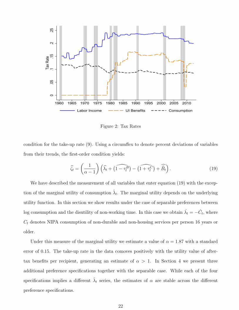
Figure 2 shows our estimated tax series τwt , τBt , and τCt . The series exhibit sharp movements

around legislated tax changes. For example, UI benefits become partially federally taxable in

1979 and fully taxable as part of the Tax Reform Act of 1986. The sharp drop in τBt in 2009

reflects the exemption of the first $2,400 of UI income from federal adjusted gross income in

that year. The secular increase in τwt until 2000 reflects mostly the increase in FICA tax rates.

Both τwt and τBt decline as a result of the Bush tax cuts in the early 2000s.12

3.4 Benefit Take-Up Cost Function

Our final input into equation (11) is the elasticity of the cost of take-up ψ(ζt) with respect to

the take-up rate ζt, which we denote by α = ψ′(ζt)ζt/ψ(ζt). We estimate α using the first-order

11Following the availability of tax law in TAXSIM, we include state taxes beginning in 1977. We extrapolateboth τst and τBt for 2009-2012 using the fitted values from a regression of the tax rates as computed using the IRSPublic Use Files on the tax rates computed using the same methodology but with the March CPS as the microdata.

12Our series for τwt correlates highly with an effective labor income tax rate series calculated from NIPA sources.After extending the methodology of Mendoza, Razin, and Tesar (1994) to our longer sample, the R-squared froma regression of the one series on the other exceeds 85 percent.

21

0.0

5.1

.15

.2.2

5Ta

x Rat

e

1960 1965 1970 1975 1980 1985 1990 1995 2000 2005 2010

Labor Income UI Benefits Consumption

Figure 2: Tax Rates

condition for the take-up rate (9). Using a circumflex to denote percent deviations of variables

from their trends, the first-order condition yields:

ζt =

(1

α− 1

)(λt + (1− τBt )− (1 + τCt

)+ Bt) . (19)

We have described the measurement of all variables that enter equation (19) with the excep-

tion of the marginal utility of consumption λt. The marginal utility depends on the underlying

utility function. In this section we show results under the case of separable preferences between

log consumption and the disutility of non-working time. In this case we obtain λt = −Ct, where

Ct denotes NIPA consumption of non-durable and non-housing services per person 16 years or

older.

Under this measure of the marginal utility we estimate a value of α = 1.87 with a standard

error of 0.15. The take-up rate in the data comoves positively with the utility value of after-

tax benefits per recipient, generating an estimate of α > 1. In Section 4 we present three

additional preference specifications together with the separable case. While each of the four

specifications implies a different λt series, the estimates of α are stable across the different

preference specifications.

22

0.0

2.0

4.0

6.0

8.1

.12

Oppo

rtunit

y Cos

t Rela

ted

to V

alue

of B

enef

its

1960 1965 1970 1975 1980 1985 1990 1995 2000 2005 2010

Figure 3: Time Series of b Component of Opportunity Cost

3.5 Results

We now combine our measurements of the various components to calculate a time series of b

using equation (11).13 We normalize b and other variables by expressing them relative to the

mean level of the after-tax marginal product of employment pτ . Denoting total output by Yt and

the pre-tax marginal product of employment by pt = ∂Yt/∂et, we define the after-tax marginal

product of employment as pτt = pt (1− τwt ) /(1 + τCt

), where τwt is the labor income tax rate

and τCt is the tax rate on consumption. We normalize its mean value to pτ = 1.14

In Figure 3 we present the time series of b relative to the mean after-tax marginal product

of employment pτ = 1. Our estimated b is countercyclical and very volatile, mostly reflecting

the significant increase in UI eligibility and take-up during recessions. The correlation between

the cyclical component of b and the cyclical component of real GDP per capita is -0.45. The

standard deviation of the cyclical component of b is roughly 6 times larger than the standard

13To make this equation operational in the data, we drop the expectations operator and substituteβλt+1(1+τC

t )λt(1+τC

t+1)=

11+rt+1

. We measure rt+1 using the interest rate on 10-year U.S. Treasuries less a measure of expected inflation.14Let Yt = Ft(Kt, etNt) be a constant returns to scale aggregate production function. We set to ν = 0.333 the

elasticity of output with respect to capital. We measure the pre-tax marginal product of employment, pt, as 1− νmultiplied by real GDP and then divided by the number of employed. The marginal product of total labor hours isgiven by xt = ∂Yt/∂(etNt) = pt/Nt. We use a superscript τ to also denote the after-tax marginal product of totallabor xτt = xt (1− τwt ) /

(1 + τCt

). We normalize mean hours per worker to N = 1 and therefore xτ = 1.

23

deviation of the cyclical component of real GDP per capita.

A key finding that emerges from our analysis is that the mean level of b is small. We find that

the mean b in our sample is roughly 6 percent of the after-tax marginal product of employment

pτ . This estimated level of b is much smaller than the values typically used in calibrated versions

of the MP model.15

What explains our estimate? Beginning with the UI component of b, the sample mean of

pre-tax benefits per recipient, B, is 21.5 percent of the pre-tax marginal product p and 30

percent of the after-tax marginal product pτ .16 However, on average only about φ = ωζ = 40%

of unemployed actually receive benefits. Therefore, pre-tax benefits per unemployed Bu =

φB equal 12 percent of the after-tax marginal product. After-tax benefits per unemployed,

(1−τB)Bu/(1+τC), equal roughly 10 percent of the after-tax marginal product. The expiration

of benefits reduces the value of UI benefits to 8 percent of the after-tax marginal product and

take-up disutility costs further reduce the value of UI benefits to 4 percent of the after-tax

marginal product. Finally, adding the Bn component yields b = 0.06. To summarize our

calculations for the mean level of b, we show in equation (20) how each term contributes to our

estimate:

b = Bn︸︷︷︸0.02

+ Bu︸︷︷︸0.12

(1− τB

1 + τC

)︸ ︷︷ ︸

0.83

(1− 1

α

)︸ ︷︷ ︸

0.47

[bracket in eq. (11)]︸ ︷︷ ︸0.83

= 0.06. (20)

4 Measurement of the ξ Component

We now turn to the value of non-working time relative to consumption ξ. To measure ξ we

use equation (12) and proceed in three steps. First, we specify utility functions. Second, we

15The sensitivity of reported reservation wages to UI benefits suggests one respect in which our b may still betoo large. In our model, the increase in the reservation wage for individuals already receiving UI is given by thetax-adjusted bracketed term in equation (11), which has a sample average value of roughly 0.69. Estimates of theincrease in reservation wages when UI benefits increase range from zero (Krueger and Mueller, 2013) to as large as0.42 (Feldstein and Poterba, 1984).

16A rate of 21.5 percent accords well with the benefit levels used by Mortensen and Nagypal (2007) and Halland Milgrom (2008) and the rate suggested by Hornstein, Krusell, and Violante (2005). The Department of Laborestimates a wage replacement rate of about 45 percent (http://workforcesecurity.doleta.gov/unemploy/ui_replacement_rates.asp, accessed 2/15/2015). Converting a wage replacement rate of 45 percent to a totalcompensation replacement rate requires multiplying by the ratio of wages to total compensation, or a factor ofabout 0.8. The remaining difference can be explained by the gap between compensation and the marginal productand from differences in productivity and compensation between those receiving UI and the economy-wide average.We address the issue of heterogeneity in Section 6.

24

measure in the data the consumption of the employed and unemployed and hours per worker.

Third, we use our estimates of consumptions and hours to calibrate preference parameters and

time endowments, which are used as inputs into the measurement of ξ.

4.1 Preferences and Time Endowments

Flow utility is a function of a bundle of consumption and working time, U s(Cs, N s), for each

employment status s ∈ {e, u}. We let N et = Nt denote hours worked by the employed and

Nut = 0 denote hours worked by the unemployed. Denote by Lu the (constant) endowment of

time that unemployed spend on leisure and home production activities. Denote by T any fixed

time cost associated with working. Time spent on leisure and home production by the employed

is, therefore, given by Let = Lu − T −N et .

We measure the ξ component of the opportunity cost for each of three widely-used utility

functions:

SEP: U st = log (Cs

t )−χε

1 + ε(N s

t + T )1+1ε , (21)

CFE: U st =

1

1− ρ

((Cs

t )1−ρ(

1− (1− ρ)χε

1 + ε(N s

t + T )1+1ε

)ρ− 1

), (22)

CD: U st =

1− χ1− ρ

(Cst )

1−ρ (Lst )χ(1−ρ)1−χ . (23)

The first two utility functions feature a constant Frisch elasticity of labor supply along the

intensive margin, ε, in the absence of fixed time costs T = 0. The utility function in equation

(21), denoted by “SEP,” is separable between consumption and hours. The preferences defined

in equation (22), labeled “CFE,” allow for non-separability between consumption and hours

worked.17 CFE preferences nest SEP preferences when ρ = 1. With ρ > 1, consumption and

non-working time are substitutes and the consumption of the employed exceeds the consump-

tion of the unemployed. The Cobb-Douglas (“CD”) utility function in equation (23) explicitly

introduces leisure and home production time in the utility function of the unemployed. CD

preferences feature a non-separability between consumption and non-working time, but they do

not admit a constant Frisch elasticity even when T = 0.

17See Shimer (2010) and Trabandt and Uhlig (2011) for further discussion of these preferences.

25

4.2 Consumption

For non-separable preferences, the measurement of ξ requires time series of consumptions of the

employed Cet and the unemployed Cu

t . Let s ∈ {e, u, n, r} denote persons 16 years or older who

are employed, unemployed, out of the labor force but of working age (16-64), and older than 65

years old, respectively. Let πst be the fraction of the population belonging in each group. Time

series of πst come directly from published tabulations by the BLS.

Denote by Cst consumption expenditure on nondurable goods and non-housing services per

member of group s. We have the adding-up identity:

πetCet + πut C

ut + πnt C

nt + πrtC

rt = CNIPA

t , (24)

where CNIPAt is NIPA consumption of nondurable goods and non-housing services per person

16 years or older. Defining γst = Cst /C

et as the ratio of consumption in status s to consumption

when employed, we solve equation (24) for the consumption of an employed:

Cet =

CNIPAt∑s π

stγ

st

. (25)

Equation (25) together with estimates of the consumption ratios γst provide the basis for deriving

the time series of consumptions for the employed and unemployed and for calibrating the utility

functions in Section 4.4.

We now turn to our estimates of the consumption ratios γst . Let Csi,k,t denote the instanta-

neous expenditure on consumption category k of an individual i in group s at time t. When

employed, individual i has expenditure Cei,k,t = exp {φk,tXi,t + εk,i,t} Ck,t, where Xi,t denotes a

vector of demographic characteristics, φk,t a vector of parameters, εk,i,t a mean zero idiosyn-

cratic component uncorrelated with employment status, and Ck,t a base level of consumption.

For every s ∈ {e, u, n, r}, we use the definition of γsk,t and obtain:

Csk,i,t = γsk,t exp {φk,tXi,t + εk,i,t} Ck,t. (26)

For a working age individual with potential status e, u, or n, we integrate over the reporting

period and take logs to obtain:

lnCk,i,t = γ0k,t + φk,tXi,t +(γuk,t − 1

)Dui,t +

(γnk,t − 1

)Dni,t + εk,i,t, (27)

26

where γ0k,t = ln Ck,t and the variables Dui,t and Dn

i,t measure the fraction of time an individual

spends as unemployed and out of the labor force, respectively.18 In equation (27), γsk,t − 1

denotes the difference between the log consumption of an individual in group s and the log

consumption of an employed. Therefore, to recover the actual consumption ratios γsk,t from the

log point differences we use the formula γsk,t = exp(γsk,t − 1

).

We begin by estimating equation (27) using the Consumer Expenditure Survey (CE). The

CE asks respondents for the number of weeks worked over the previous year, but does not ask

questions about search activity while not working. We set Dni,t = 1 if the respondent reports

zero weeks worked over the previous year and does not give “unable to find job” as the reason

for not working. For the rest of the respondents, we define Dui,t = 1 − (weeks worked)i,t /52.

We average Dui,t and Dn

i,t at the household level. To minimize inclusion of households with

adults transitioning out of the labor force within the reporting year, we restrict the sample to

households with a head age 30 to 55 at the time of the final interview. We include a rich set of

controls in Xi,t to control for taste shocks and ex-ante permanent income that potentially could

correlate with an individual’s employment status.19

We focus our discussion of results on the unemployment margin because γu will directly

inform our calibration of preferences. Figure 4 reports γu by year, for the aggregate category

of nondurable goods and services, less housing, health, and education. The mean of γu implies

a 21 percent decline in expenditure on nondurable goods and services during unemployment.

The series does not exhibit any apparent cyclicality, with a correlation between the cyclical

components of γu and the unemployment rate of -0.03. We also test for cyclicality parametrically

18In deriving our estimating equation we replace the term ln[1−

∑s

(1− γsk,t

)Dsi,t

]with

∑sD

si,t

(γsk,t − 1

),

where the coefficients γsk,t are related to the coefficients γsk,t and to terms of order higher than one in the linearapproximation of the left-hand side around γsk,t = 1,∀s. Derivations for the estimating equation for γrt proceedanalogously. The derivation of equation (27) assumes that γuk,t does not vary with unemployment duration Du

i,t.In unreported regressions, we have estimated γuk,t non-parametrically by grouping households into bins of weeksunemployed. Our estimated γuk,t for each bin indicates a duration-independent γuk,t. This finding supports theassumption in the model that the instantaneous consumption of the unemployed does not depend on duration.

19These controls include: the mean age of the household head and spouse; the mean age squared; the maritalstatus; an indicator variable for Caucasian or not; indicator variables for four categories of education of thehousehold head (less than high school, high school diploma, some college, college degree) interacted with year;indicator variables for owning a house without a mortgage, owning a house with a mortgage, or renting a house,interacted with year; indicator variables for quantiles of the value of the home conditional on owning, by regionand year, interacted with year; a binary variable for having positive financial assets; family size; and family sizesquared.

27

.4.6

.81

C tu /

C te

1985 1990 1995 2000 2005 2010

Figure 4: Decline in Nondurables and Services Upon Unemployment

Notes: The solid line reports the estimates of γut = exp(γu,t − 1), where γu,t is estimated from equation (27) usingdata from the CE. The dotted lines give 95 percent confidence interval bands based on robust standard errors.Regressions are weighted using survey sampling weights. See footnote 19 for included covariates.

by interacting Dui,t in equation (27) with both the state and national unemployment rates and

again cannot reject the hypothesis that the consumption ratio is acyclical (see Table 2).

The cross-sectional identification in equation (27) relies on the richness of the control vari-

ables to absorb differences in ex-ante permanent income. We complement this approach with

panel regressions relying on within household changes in consumption. First differencing equa-

tion (27) to remove the individual fixed effect we obtain:20

∆ lnCk,i,t = ∆γ0k,t +∑

s∈{u,n}

[(γsk,t − 1

)∆Ds

i,t + ∆γsk,tDsi,t−1

]+ ∆εi,k,t, (28)

We use the panel dimension of the PSID to estimate equation (28).21 Table 2 reports esti-

mates of γuk from equation (27) for the CE and from equation (28) for the PSID. For total food,

the PSID suggests a somewhat larger γuk than the CE, but this may reflect an upward bias in

20In deriving equation (28), we impose that φk,t = φk. In unreported results, we have also estimated equation(28) by interacting a set of controls with year categorical variables and find that the PSID results in Table 2 remainessentially unchanged.

21The PSID asks detailed questions about labor force status. We use these to construct the frac-tion of the reporting period in unemployment in a manner analogous to the BLS U-3 definition, Du

i,t =[weeks searching or on temporary layoff in year t

weeks in the labor force in year t

]i. This more precise definition of unemployment constitutes an additional

dimension along which the PSID provides robustness for the CE results.

28

Table 2: Relative Expenditure of the Unemployed γu

Total food Food, clothing Nondurablesrecreation, vacation and services

CE PSID CE PSID CEγu 0.79 0.86 0.72 0.73 0.77

(0.013) (0.045) (0.015) (0.096) (0.012)pval (γ

u ⊥ U state, Unat.) 0.88 0.42 0.89 0.25 0.63Observations 53,413 31,616 53,413 4,871 53,413

Notes: The parameter γu gives the log point difference between the expenditure of an unemployed and the expen-diture of an employed. The CE columns cover reporting years 1983-2012. The category nondurables and servicesin the last column excludes expenditures on housing, health care, and education. The PSID columns cover re-porting years 1983-86, 1989-1996, 1998, 2000, 2002, 2004, 2006, 2008, and 2010 for food and years 2004, 2006,2008, and 2010 for clothing, recreation, and vacations. Equation (27) is used for the CE and equation (28) isused for the PSID. Regressions are weighted using sampling weights. Standard errors are in parentheses and arebased on heteroskedastic robust (CE) or heteroskedastic robust and clustered by household head (PSID) variancematrix. pval (γ

u ⊥ U state, Unat.) reports the p-value of a joint test that interacting Dui,t with the state and national

unemployment rates in equation (27) or (28) yields coefficients equal to zero.

the PSID.22 We also exploit the new questions in the PSID covering broader measures of con-

sumption expenditure. Here the estimated γuk from the PSID appears nearly indistinguishable

from the γuk from the CE for the same set of categories. The overall similarity between the

CE and the PSID results suggest that the control variables in Xi,t proxy well for differences in

ex-ante permanent income. Because of non-homotheticities across consumption categories, our

preferred results come from the CE for total nondurable goods and services less housing, health,

and education, reported in the last column of the table.

Our estimate of the consumption drop upon unemployment lies comfortably within the range

of those found in previous studies. In an early assessment, Burgess, Kingston, St. Louis, and

Sloane (1981) report in a survey of UI recipients after five weeks of unemployment that expendi-

22The PSID asks about “usual” weekly expenditure on food at home and then about food away from home withoutprompting a frequency. These questions leave some ambiguity as to whether the food expenditure questions applyto the time of the interview or to the previous year. We follow the recent literature in mapping the questions tothe previous year’s expenditure (Blundell, Pistaferri, and Preston, 2008). However, if some respondents’ interpretthe question as referencing food expenditure at the time of the interview, the resulting measurement error inunemployment status would bias the estimated γk in the PSID regressions upward. Additionally, while the CEasks about detailed categories every three months, the PSID asks about the broad categories of food at homeand food away and over a longer recall period. Hence even if respondents interpret the question as referring tothe previous year, recall bias may cause their response to partly reflect their current consumption patterns. Thenewer PSID expenditure questions on clothing, recreation, and vacation explicitly reference the previous year asthe reporting period. The smaller difference between CE and PSID for these categories is consistent with referenceperiod ambiguity introducing a bias into the PSID food results.

29

ture on the categories of food, clothing, entertainment, and travel fell by 25.7 percent relative to

before the unemployment spell. Gruber (1997) reports a decline in food expenditure of 6.8 per-

cent in the PSID for the period up to 1987. The difference between his results and ours mostly

stems from the removal of households with a threefold change in consumption from his sample.

Using a survey of Canadians unemployed for six months that asks about total expenditure over

the previous month as well as expenditure in the month before unemployment, Browning and

Crossley (2001) find a mean decline of 14 percent. Aguiar and Hurst (2005) report a 19 per-

cent decline in food expenditure among the unemployed using scanner data. Stephens (2004)

conducts an analysis of the effects of job loss on consumption in the Health and Retirement

Survey (HRS) and the PSID and finds a decline in food expenditure between 12 (PSID) and

15 (HRS) percent when an individual experiences a job loss between interviews. Finally, using

cross-sectional variation in the PSID, Saporta-Eksten (2014) estimates an 8 percent decline in

consumption expenditure on selected categories in the year in which a job loss occurs. However,

Saporta-Eksten (2014) does not condition on the fraction of the year spent out of work. To

convert the 8 percent estimate into an instantaneous consumption decline requires adjusting by

the fraction of the year spent jobless. Assuming an average unemployment duration of 17 weeks

would imply a consumption decline of roughly 24 percent, in line with our estimate. A similar

type of adjustment applies to the Stephens (2004) estimate.

We apply our estimates of the consumption ratios in two steps. First, the calibration of

preference parameters in Section 4.4 requires data on the mean level of Cet (denoted by Ce)

and the mean level of Cut (denoted by Cu). For these means, we impose constancy of the

consumption ratios γst = γs in equation (25) and obtain a time series for Cet and Cu

t = γuCet .

23

We then define Ce = (1/T )∑

tCet and Cu = (1/T )

∑tC

ut . Second, obtaining a time series of

ξt requires a time series of Cet and Cu

t . We jointly impose the adding-up constraint for total

consumption in equation (24) and the risk-sharing condition in equation (7) to solve for the

time series of Cet and Cu

t . This approach ensures the internal consistency of our estimated

23We set γu = 0.793, the value from estimating equation (27) for a constant γu. For the other categories, weestimate γn = 0.743 and γr = 0.940. Similarly to our estimates of γu, we cannot reject acyclicality of theseconsumption ratios. We also use the same time-invariant γn = 0.743 and γr = 0.940 when estimating the timeseries of Cet and Cut .

30

3839

4041

Hou

rs p

er W

orke

r

1960 1965 1970 1975 1980 1985 1990 1995 2000 2005 2010

CRK Official CPS

Figure 5: Hours Per Worker

parameters with the model’s analog of the first-order condition for risk sharing in the data. The

time-varying consumption ratio Cut /C

et implied by this procedure is extremely smooth, falling

comfortably in the confidence interval of the estimated γut .24

4.3 Hours Per Worker

The next input for the measurement of ξ is hours per worker Nt. We measure Nt as the average

weekly hours reported in the basic monthly CPS microdata by the employed. These data start

in 1968. We extend the series back to 1961 and fill in some missing months between 1968

and 1975 using data from Cociuba, Prescott, and Ueberfeldt (2012). We seasonally adjust the

series by first estimating an ARMA model including categorical variables for each month of the

year and months in which each of Good Friday, Easter Monday, Labor Day, Columbus Day, or

Veteran’s Day occurred during the CPS reference week. Then we apply a multi-step moving

average filter similar to that contained in X-11. Appendix B.1 provides further details on the

seasonal adjustment.

24The model-generated consumption ratio is mildly countercyclical because hours per worker are procyclical andconsumption and non-working time are substitutes in the utility functions we consider. Alternatively, imposingconstancy of the ratio Cut /C

ut = γu = 0.793 and using this constant ratio and equation (24) to solve for the time

paths of Cet and Cut does not change our results.

31

Figure 5 shows the resulting hours series (“CRK”). Hours per worker are procyclical. The

figure also shows the official BLS series from the CPS for comparison. During the overlapping

period 1976-2012, the cyclical component of our CRK series displays a correlation of 0.96 with

the “Official CPS” series.25

4.4 Parameterization

We now use our estimates of consumptions and hours to calibrate four models. The first model

features SEP preferences and has no fixed time costs (T = 0). The second model features CFE

preferences and also has T = 0. The third model features CD preferences, a definition of non-

working time of unemployed Lu that excludes some time uses, and T = 0. The fourth model

also features CD preferences, but adopts the most extreme view of what could be considered

utility-enhancing leisure of unemployed Lu and allows for fixed time costs T > 0. The purpose

of the fourth model is to try to rationalize the level of the opportunity cost z = 0.955 advocated

by Hagedorn and Manovskii (2008).

In general, our calibration strategy involves choosing two parameters to make two first-

order conditions hold exactly at the mean values of the variables in the sample. The first

condition is the risk-sharing condition (7) requiring the equalization of the marginal utility of

consumption between the employed and unemployed. For this condition, we use the mean values

of consumptions estimated in Section 4.2, Ce = 0.681 and Cu = 0.540. The second condition is

an efficiency condition for the choice of hours per worker, evaluated at mean sample values:

− ∂U(Ce, N)

∂N= λ

(1− τw

1 + τC

)x, (29)

where x denotes the marginal product of total labor hours. In equation (29) we use the mean

sample values of τC = 0.096 and τw = 0.209 and we have normalized N = 1.26

25The “Official CPS” series used in the above figure is the BLS seasonally adjusted hours per worker seriesLNS12005054. The BLS also offers a seasonally unadjusted series of hours per worker for nonagricultural industriesthat starts in 1948 (LNU02033120). After applying our seasonal adjustment to this alternative series, we find acorrelation of 0.98 between the cyclical component of our CRK series and the cyclical component of this alterna-tive series. We prefer using the CRK series as a baseline for comparability with our later analyses that requiremeasurement of hours per worker by educational group.

26Our measurement of ξ does not require equation (29) to hold in any particular period. We require equation(29) only in the steady state of the model in order to calibrate preference parameters. This equation arises as afirst-order condition, for example, under Nash bargaining. We view such an equilibrium as a desirable outcome in

32

Table 3: Parameterization of Preferences

Parameters Elasticities

Preferences Lu T ε χ ρ α SE(α) −1/ελC εNw εNλ −εNC

SEP 0.00 0.70 1.48 1.87 0.15 1.00 0.70 0.70 0.70

CFE 0.00 0.70 1.22 1.52 1.86 0.14 0.66 0.70 0.46 0.70

CD1 2.64 0.00 0.71 1.25 1.86 0.15 0.80 1.10 3.07 3.85

CD2 4.33 0.19 0.82 1.19 1.86 0.15 0.84 1.82 6.43 7.63

The left panel of Table 3 presents our parameterization. For the SEP preferences, the

risk-sharing condition always implies Cet = Cu

t = Ct. Thus, with perfect risk sharing, these

preferences cannot match the consumption decline at unemployment. We follow Pistaferri

(2003) and Hall (2009) and set the Frisch elasticity of labor supply to ε = 0.7. We then choose

χ = 1.48 to make equation (29) hold exactly at the mean values of the variables in the sample.

The right panel shows the elasticities implied by our parameterization. The intertemporal

elasticity of substitution in consumption is −1/ελC = 1 and the Frisch elasticity of labor supply

is εNw = ε = 0.7. The elasticity of hours with respect to the marginal utility (holding the

wage constant) is εNλ = 0.7. Finally, the elasticity of hours with respect to consumption is also

−εNC = −εNλελC = 0.7. The latter two elasticities measure wealth effects on hours along the

intensive margin.27

For the CFE preferences we again set ε = εNw = 0.7. The solution of equations (7) and

(29) gives values of χ = 1.22 and ρ = 1.52. The intertemporal elasticity of substitution in

consumption is −1/ελC = 1/ρ = 0.66. The elasticity of hours with respect to the marginal

the long run, as any other equilibrium would imply that firms and workers coordinate at an inefficient allocation.See Shimer (2010) for a similar argument in a model without taxes (page 53, footnote 6).

27The mapping of the elasticities εNλ and εNC into the elasticity of hours with respect to income εNY (whichhas a more direct mapping to empirical studies) requires specifying the income process and structure of the capitalmarkets. For example, if shocks are relatively transitory and workers can access capital markets to smooth suchshocks, then consumption and λ will not change much in response to income shocks, making εNY small. Theopposite holds if shocks are permanent or borrowing possibilities are restricted.

33

utility of wealth is εNλ = ε/ρ = 0.46 and with respect to consumption is εNC = 0.70.28

For CD preferences, we additionally need an estimate of the time endowment of the unem-

ployed Lu. Using the American Time Use Survey (ATUS, 2003-2012), we find that unemployed

spend 47.6 hours per week on leisure activities (for example, watching TV, listening to music,

and socializing with friends), 16.5 hours per week on discretionary sleeping time (defined as

the excess sleeping time over 49 hours), 24.6 hours per week on home production (for example,

cooking, home ownership activities, and shopping), 6.9 hours per week on child care, and 7 hours

per week on activities such as education, religious activities, and own medical care. Dividing

the sum of these hours (102.6) by hours per worker (38.8), we obtain Lu = 2.64 relative to a

mean value of N = 1.

In Table 3, the row labeled “CD1” presents our parameterization when Lu = 2.64 and there

are no fixed time costs associated with working (T = 0). The row labeled “CD2” presents an

alternative parameterization of CD preferences which yields the level of z = 0.955 advocated by

Hagedorn and Manovskii (2008). This parameterization sets Lu = 4.33, corresponding to the

broadest view that all 168 hours per week potentially constitute utility-enhancing non-working

time. It also requires fixed time costs of working equal to 19 percent of average hours per

worker.29 As Table 3 shows, both sets of CD preferences feature a higher Frisch elasticity of

labor supply than the SEP and CFE calibrations. The CD preferences also imply much stronger

wealth effects on hours than SEP and CFE preferences.

Table 3 also presents estimates of the elasticity of the cost function with respect to take up,

α, from an OLS regression of equation (19), along with Newey-West standard errors with four

lags. The four preference specifications imply different λt series. However, the estimates of α

are stable across the different preference specifications.

28These values are close to the values used in Hall (2009), with the small difference mostly reflecting that ourestimated ρ is lower than the ρ implicit in Hall’s formulation. See Hall’s Appendix for a summary of evidence onthese elasticities. In general, the CFE calibration comes closer to matching the evidence cited in Hall than theSEP, CD1, and CD2 calibrations.

29A value of T = 0.19, implying fixed costs of more than 7 hours per week, appears quite large relative to typicalestimates of commuting time. Rogerson and Wallenius (2013) review evidence on commuting time and find thatT is approximately 0.1. Rogerson and Wallenius (2013) also point out that commuting time does not constitute afixed cost if individuals adjust the number of days at work rather than hours per day, making T = 0.1 an upperbound under this interpretation of the fixed cost. In our robustness checks we consider an alternative model inwhich fixed costs are denominated directly in terms of utility rather than time.

34

4.5 Results

Combining our estimates of consumption by labor force status and hours per worker with our

calibrated utility functions, we now estimate a time series of ξ according to equation (12). For

each of the four calibrated models, we first discuss the estimated levels of ξ. Then, we discuss

the cyclicality of ξ.

We obtain the following levels of ξ (relative to an after-tax marginal product of employment

pτ = 1):

ξSEP = 0.41, ξCFE = 0.41, ξCD1 = 0.70, ξCD2 = 0.90. (30)

We begin our analysis by considering the steady state value of ξ under the SEP and CFE

specifications:30

ξSEP = ξCFE =

(ε

1 + ε

)pτ . (31)

For a value of ε = 0.7, we obtain ξSEP = ξCFE = 0.41 relative to the after-tax marginal product

of pτ = 1. A higher Frisch elasticity of labor supply results in a higher level of opportunity

cost. However, using these utility specifications, one would need to assume a Frisch elasticity

of 9 to rationalize a level of ξ equal to 0.90. Could, alternatively, fixed time costs explain such

a high level of ξ under SEP or CFE preferences? Introducing fixed time costs changes the level

to ξSEP = ξCFE = pτ (1 +T/N)ε/(1 + ε). It also changes the Frisch elasticity to (1 +T/N)ε. For

T roughly equal to 120 percent of N , one would estimate ξ = 0.90 with a less extreme Frisch

elasticity of 1.54. However, the magnitude of these fixed costs is implausible.

In the absence of fixed time costs (T = 0), we can write ξ under CD preferences as a function

of the endowment of non-working time of the unemployed Lu:

ξCD =

(1− γu

− log(γu)

)(Lu − 1) log

(Lu

Lu − 1

)pτ , (32)

where γu = 0.793 is the consumption of the unemployed relative to the employed. We obtain

that limLu→1 ξCD = 0, limLu→∞ ξ

CD =(

1−γu− log(γu)

)pτ = 0.89, and that between these limiting

30The Appendix to Hall (2014) first derives this equation for SEP preferences. The equation results from substi-tuting the condition for hours in equation (29) into the expression for ξ in equation (12). Because our measurementexercise does not require that equation (29) holds in any particular period, equation (31) need not hold period-by-period.

35

cases ξCD is an increasing function of the endowment of time Lu. Our estimate of Lu = 2.64

under calibration CD1 yields ξCD = 0.70. Model CD2 implies a higher value of ξ both because we

calibrate the endowment of time at the higher level of Lu = 4.33 and because we introduce fixed

time costs associated with working T = 0.19. Without fixed time costs but with Lu = 4.33,

we would have estimated ξ = 0.78. Therefore, of the 20 percentage point difference in ξ

between calibration CD2 and calibration CD1, 12 percentage points are due to fixed costs and

8 percentage points are due to the higher level of the time endowment.31

To summarize, our estimated levels of ξ differ substantially across specifications. We show

how the level of ξ depends on the underlying utility function, the estimated time endowment of

the unemployed, and fixed costs associated with working.32 Despite these meaningful differences,

we now show that the cyclicality of ξ is quite stable across different specifications.

Figure 6 shows the percent deviation of ξ from its trend. We compute trends of variables

using the HP filter with a smoothing parameter of 1,600. We see that all four specifications

result in highly similar cyclical components of ξ. In particular, all four specifications imply a

procyclical and volatile ξ.

To develop intuition about the cyclicality of ξ, it is useful to consider the SEP utility function.

Under SEP we obtain:

ξSEPt =

(χε

1 + ε

)N

1+ 1ε

t Ct. (33)

The ξ component of the opportunity cost is procyclical because in the data both hours per

worker and consumption are procyclical.33 The intuition for the cyclicality of ξ in the SEP

31Using a narrower definition of leisure and home production that roughly corresponds to the time uses definedin Aguiar, Hurst, and Karabarbounis (2013) we obtain Lu = 2.00 and ξ = 0.62. Our inference about the cyclicalityof z in this case is not very different than in the CD1 and CD2 cases. For example, we obtain an elasticityε (z, p) = 0.87 as opposed to values of 0.85 and 0.83 under CD1 and CD2 respectively.

32If flow utilities were equalized, Uu = Ue, then we would have obtained ξ = Ce−Cu. In this case, our estimatesof consumption differences imply that ξ = 0.14. A higher level of ξ requires (Uu − Ue)/λ > 0. The interpretationof (Uu−Ue)/λ > 0 is that non-working time is valued at a sufficiently high level relative to consumption, which isa standard assumption in the literature (see Rogerson and Wright, 1988). In the model with incomplete marketsdiscussed in Appendix C, the unemployed’s expected sum of discounted utility flows V u is lower than the employed’sexpected sum of discounted utility flows V e, even when flow utilities satisfy Uu > Ue.

33Our preferred measure of consumption CNIPAt in this paper excludes durables and housing services. At quarterly

frequency and using a HP filter with smoothing parameter of 1,600 to detrend variables, the volatility of the cyclicalcomponent of CNIPA

t relative to the volatility of the cyclical component of real GDP per person 16 years or olderis 0.66. However, the stock of durables is also volatile over the business cycle. The relative volatility of the cyclicalcomponent of the real stock of durables is 0.73.

36

-.04

-.02

0.0

2.0

4Pe

rcen

t Dev

iation

from

Tre

nd

1960 1965 1970 1975 1980 1985 1990 1995 2000 2005 2010

ξ SEP ξ CFE ξ CD1 ξ CD2

Figure 6: Cyclical Components of ξ

Notes: Variables are logged and HP filtered with a smoothing parameter of 1,600.

case carries over to the other preference specifications. In all cases, procyclical hours and

consumption imply a procyclical ξ component of the opportunity cost. Quantitatively, ξ is less

volatile in the non-separable specifications because, with procyclical hours, the complementarity

in preferences between consumption and hours ameliorates the cyclicality of the marginal utility

of consumption λ.

5 The Opportunity Cost of Employment in the Data

We now combine our measurements of the two components, b and ξ, and describe the properties

of the opportunity cost of employment z = b+ ξ.

5.1 Baseline Results

Table 4 presents summary statistics for the period 1961(1) to 2012(4) for each set of preferences.

The level of z ranges between 0.47 and 0.96 of the after-tax marginal product of employment

pτ . The variation in the average level of z across preferences reflects the variation in the average

level of the component of the opportunity cost associated with the value of non-working time

ξ. In all cases, ξ constitutes the largest part of z, ranging between 0.41 and 0.90.

37

Table 4: Summary Statistics, 1961(1) to 2012(4)

Statistic SEP CFE CD1 CD2

pτ 1.00 1.00 1.00 1.00p 1.39 1.39 1.39 1.39z 0.47 0.47 0.75 0.96ξ 0.41 0.41 0.70 0.90b 0.06 0.06 0.06 0.06

sd(Y)

1.50 1.50 1.50 1.50

sd (p) 0.89 0.89 0.89 0.89sd (z) 1.66 1.52 1.19 1.10

sd(ξ)

1.92 1.63 1.29 1.20

sd(b)

8.97 8.95 8.96 8.96

corr(z, Y

)0.52 0.42 0.55 0.61

corr(ξ, Y

)0.87 0.87 0.86 0.86

corr(b, Y

)−0.45 −0.45 −0.45 −0.45

ε (z, p) 1.11 0.92 0.85 0.83CI [0.74,1.49] [0.56,1.28] [0.59,1.11] [0.60,1.06]

Notes: We denote the percent deviation of some variable xt from its trend by xt. We compute trends of variablesusing the HP filter with smoothing parameter of 1,600. The elasticity ε (x1, x2) is the regression coefficient of x1

on x2. Newey-West standard errors with four lags are in parentheses.

Turning to the cyclicality of the opportunity cost, Figure 7 plots the percent deviation of z

from its trend for each of the four parameterizations. The four series track each other closely.

All appear to be procyclical, falling during each recession in our sample. Table 4 confirms that

z comoves positively with real GDP per capita Y over the business cycle. It also shows that z

is quite volatile over the business cycle, with the standard deviation of its cyclical component

exceeding the standard deviation of the cyclical component of the marginal product p.

The procyclical movement of z reflects the dominance of the ξ component in the sum z = b+ξ.

As discussed before and summarized in Table 4, the b component is countercyclical and very

volatile. However, the small level of b makes its fluctuations relatively unimportant for z.

Table 4 also reports the elasticity of z with respect to p as a metric that takes into account

both the correlation between the two variables and the relative volatilities. As we show below,

38

-.06

-.04

-.02

0.0

2.0

4Pe

rcen

t Dev

iation

from

Tre

nd

1960 1965 1970 1975 1980 1985 1990 1995 2000 2005 2010

z SEP z CFE z CD1 z CD2

Figure 7: Cyclicality of Opportunity Cost of Employment

Notes: Variables are logged and HP filtered with a smoothing parameter of 1,600.

this elasticity is an informative statistic for the magnitude of unemployment fluctuations in a

wide class of models. For consistency with prior literature that focuses on TFP shocks as the

driving force in business cycle models and to correct for measurement error in p, we instrument

p with the cyclical component of the Fernald (2012) unadjusted TFP series.34 The resulting

elasticities of z with respect to p range between 0.83 and 1.11. The elasticity declines when

moving from SEP to other preferences, reflecting the non-separability embedded in the other

specifications. We cannot reject the null hypothesis that the elasticity equals 1 for any of the

preference specifications. We conclude that the opportunity cost of employment moves roughly

proportionally with the marginal product of employment over the business cycle.

5.2 Sensitivity Analysis

We assess the sensitivity of the cyclicality of z to a number of modelling assumptions and use

of data moments. In Table 5, each row reports the elasticity ε(z, p) under a different alternative

scenario for each of the four preference specifications indicated in the column headings. Row

34We motivate our focus on p instead of pτ by appealing to prior literature in which productivity shocks aretreated as exogenous. Empirically, the elasticity of the cyclical component of the tax wedge (1− τw)/(1 + τC) withrespect to the cyclical component of p in our data is 0.014 (instrumented) and 0.067 (not instrumented). That is,taxes respond very little to cyclical movements in p.

39

Table 5: Sensitivity of Elasticity ε (z, p)

Case SEP CFE CD1 CD2

0. Baseline Results 1.11 0.92 0.85 0.83

1. Benefit Component bt Equal to Trend 1.32 1.13 0.98 0.93

2. Non-Working Time Component ξt Equal to Trend -0.06 -0.09 -0.02 0.00

3. Consumption CNIPAt Equal to Trend 0.52 0.33 0.22 0.19

4. Hours Nt Equal to Trend 0.54 0.46 0.57 0.60

5. Smaller Consumption Decline (γu = 0.9) 1.11 1.02 0.92 0.90

6. Hours Nt of Salary Workers 1.03 0.85 0.81 0.80

7. Hours Nt of Hourly Workers 1.21 1.00 0.90 0.87

8. Hours Nt Adjusted for Composition 1.19 0.98 0.89 0.86

9. Higher Frisch Elasticity (ε = 2) 1.01 0.86 N/A N/A

10. Alternative Model of Take-Up (ζ = 1.00) 1.01 0.85 0.82 0.82

11. No Taxes (τw = τC = τB = 0) 1.20 1.01 0.91 0.87

12. Fixed Utility Costs of Working for z = 0.96 0.96 0.91 0.85 0.84

13. Baxter-King Filter 1.17 0.97 0.91 0.88

14. No Instrumenting 1.01 0.87 0.78 0.75

15. No Instrumenting and Baxter-King Filter 1.15 0.98 0.89 0.86

0 provides the baseline elasticities. Unless otherwise noted, in each sensitivity exercise we

recalibrate all model parameters whenever necessary in order to achieve the same targets as in

our baseline procedure.

The rows in the middle panel provide further intuition for the cyclicality of z by selectively

shutting off the cyclicality of various inputs. The first row reports elasticities ε (z, p) in the

counterfactual in which the b component of z always equals its trend. The estimated elasticities

increase, reflecting the fact that b is countercyclical. However, these increases are relatively

small because b constitutes a small part of the opportunity cost. To assess the contribution of

the ξ component for z fluctuations, in the second row we set the ξ component equal to its trend.

We find that the elasticities ε (z, p) become slightly negative or zero. None of the four estimated

40

elasticities is statistically significant at the 10 percent level. Setting ξ equal to its trend implies

an acyclical z because the level of b is much smaller than the level of ξ.

Row 3 reports elasticities ε (z, p) when our underlying measure of consumption CNIPAt equals

its trend. In this counterfactual scenario, all of the elasticities decline substantially. We conclude

that the procyclicality of consumption is a major factor in generating the procyclical behavior of

z. In row 4 we set hours per worker Nt equal to its trend. The elasticities decrease, but by less

than in the scenario in which consumption equals its trend. We conclude that the procyclicality

of hours contributes to the procyclicality of z but that, quantitatively, cyclical movements in

hours per worker matter less than cyclical movements in consumption.

The bottom panel explores robustness to using other plausible data moments or modelling

assumptions. Row 5 assesses the sensitivity of the estimated elasticities to the value of the

ratio of the consumption of the unemployed relative to the employed. Our baseline calibration

of preference parameters uses the value of γu = 0.793. Row 5 instead sets γu = 0.9. With

procyclical hours, the complementarity between hours and consumption makes the marginal

utility λ less cyclical, which in turn ameliorates the procyclicality of ξ. The complementarity

in preferences becomes stronger when the consumption ratio γu is lower. Therefore, increasing

γu increases all estimated elasticities for non-separable preferences.35

Rows 6 and 7 replace Nt with series for hours per worker constructed separately for salaried

and hourly workers respectively. Hourly workers experience more procyclical hours per worker

than salary workers, explaining the larger elasticities in row 7 than in row 6. However, both types

of workers have quite volatile and procyclical hours series, leading to significant procyclicality

in z in both cases.36

In row 8 we adjust our measure of hours for compositional changes. In principle, hours

per worker could decline in recessions because economic activity reallocates toward industries

35Our baseline SEP preferences imply a unitary elasticity of intertemporal substitution. Using separable butnon-balanced growth preferences of the form U =

(C1−ρ − 1

)/(1− ρ)− (χε/(1 + ε))N1+1/ε allows us to decouple

ρ from the consumption decline upon unemployment and examine the sensitivity of our results to the assumedelasticity of intertemporal substitution. With ρ = 2, which implies an intertemporal elasticity of 1/2, we findε (z, p) = 1.77. Intuitively, for given cyclical component of consumption, increasing ρ makes λ more cyclical.

36We construct hours per worker for hourly and salary workers from the CPS monthly files. The identificationof the type of worker is possible on a continual basis only starting in 1982. Before then we impute hours for thesetwo groups based on a projection on aggregate hours.

41

or demographic groups with lower average hours. To adjust for such compositional shifts, we

regress hours of employed on industry, gender, education, and age bracket categorical variables.

We then construct hours for each worker as the sum of the regression residual and a sample

mean, aggregate these hours, and apply our seasonal adjustment procedure. The elasticities

ε (z, p) increase slightly as a result of this compositional adjustment. In practice, compositional

changes dampen rather than exacerbate cyclical movements in hours per worker.

In row 9 we increase the Frisch elasticity of labor supply for SEP and CFE preferences to

ε = 2 and recalibrate the remaining preference parameters to match the same targets as in our

baseline results. A larger ε implies a smaller effect from fluctuations of hours per worker on

fluctuations of the ξ component of the opportunity cost. However, even for ε = 2 the estimated

elasticities ε (z, p) remain close to one. We view the value of 2 as an upper bound of reasonable

values of the Frisch elasticity, given that our model has an extensive margin of labor supply.

Row 10 examines the sensitivity of our results to the assumed model of UI take-up. Motivated

by the evidence in Blank and Card (1991) and Anderson and Meyer (1997) that take-up rates are

significantly below one and respond to benefit levels, in our baseline model eligible unemployed

take up benefits when the utility value of after-tax UI benefits exceeds the utility cost of take-

up. We now consider an alternative model in which the opportunity cost of eligible unemployed

always includes the full value of their UI entitlement with no disutility. Thus, in equation (11)

we set α to infinity and ζt = 1. With this modification, the level of b increases. However, the

estimated elasticities ε (z, p) do not change much because without a take-up margin b fluctuates

much less.

In row 11, we set all taxes to zero and recalibrate all parameters in the model without taxes.

For all preference specifications we obtain larger elasticities. Taxes increase the level of b relative

to the after-tax marginal product because the tax rate on UI benefits τB is lower than the tax

rate on labor income τw. Because the b component is countercyclical, reducing its importance

in the model without taxes generates larger elasticities.

In our baseline model, under calibration CD2, we introduced fixed time costs in order to

achieve a high level of z. We now consider an alternative model in which fixed costs asso-

42

ciated with working are denominated directly in terms of utility rather than in units of time.

Specifically, each individual incurs a fixed cost FC when moving from unemployment to employ-

ment which, for simplicity, enters additively into the utility function. With this modification,

ξt is given by equation (12) plus the additive term FC/λt. For each preference specification,

we choose FC such that we obtain the mean value of z = 0.955 suggested by Hagedorn and

Manovskii (2008). As row 12 of Table 5 shows, the elasticity ε (z, p) declines somewhat relative

to our baseline results only for the SEP case.

Finally, rows 13 to 15 report the sensitivity of our results to our procedure for estimating

the elasticities ε (z, p). Row 13 uses the Baxter-King (BK) filter to separate the trend from

the cycle, using a bandwidth of 6 to 32 quarters. All elasticities increase slightly. Row 14

reports elasticities using the HP filter but without instrumenting for the marginal product.

Here the elasticities decline by 0.05 to 0.1. Finally, row 15 shows that our results remain largely

unchanged when we use the BK filter and we do not instrument for the marginal product.

To summarize, the combination of procyclical hours per worker, procyclical consumption,

and a small level of benefits b imply a procyclical and volatile opportunity cost z. Further, we

estimate that a one percent increase in p is associated with an increase in z of at least 0.8 percent

and we cannot reject the hypothesis that z and p move proportionally over the business cycle.

This result appears robust to various preference specifications, alternative data definitions, and

modeling choices.

6 Heterogeneity Across Skills

Our measurement of z for the average unemployed followed from the assumption that all un-

employed search for the same jobs and employers cannot discriminate ex-ante in choosing a

potential worker with whom to bargain. We now relax this assumption and allow workers to

differ along observable characteristics that may be correlated with their opportunity costs.

The economy consists of J heterogeneous households. In our empirical implementation

we separate workers into four educational attainment categories. Each household j contains

fraction lj of the population. Within each group j, a fraction ejt are employed and a fraction

43

ujt are unemployed. There are J segmented labor markets. We denote by fjt the job finding

rate in market j and by sjt the separation rate. Employment for group j evolves as ejt+1 =

(1− sjt)ejt + fjtujt.

The problem of each household j is:

W hj = maxE0

∞∑t=0

βt[ljejtUj(C

ejt, Njt) + lj(1− ejt)Uj(Cu

jt, 0)− lj(1− ejt)ωjtψ(ζjt)], (34)

subject to the budget constraint:

(1 + τCt

) (ljejtC

ejt + lj(1− ejt)Cujt

)+Ijt+Πjt = (1−τwjt)wjtljejtNjt+lj(1−ejt)Bjt+(rt + δ)Kjt, (35)

and the law of motion for eligibility:

ωjt+1 =

(ωujt+1(1− fjt)

ujtujt+1

)ωjt + ωejt+1sjt

ejtujt+1

. (36)

We note that flow utilities Uj are allowed to vary by j. In the budget constraint, after-tax

benefits per unemployed of type j are given by Bjt =(1 + τCt

)Bn,jt + (1 − τBtj )Bu,jt, where

Bn,jt denotes non-UI benefits per unemployed, Bu,jt denotes UI benefits per unemployed, and

τBtj denotes the UI tax rate in group j.

To derive the opportunity cost of employment by group j, we proceed analogously to the

aggregate case analyzed in Section 2. We first derive the marginal value of employment for

household j, Jhjt = ∂W hjt/∂ (ljejt), as the sum of a flow payoff (after-tax wages minus opportunity

cost) and a continuation value. Then, we define the opportunity cost of employment similarly

to the aggregate case:

zjt = bjt + (Cejt − Cu

jt)−U ejt − Uu

jt

λjt= bjt + ξjt, (37)

where bjt is given by equation (11) taking into account j-specific values of variables. The thrust

of our procedure for constructing zjt follows that for the aggregate described in Section 3. Here

we sketch briefly our estimation and refer the reader to Appendix B.2 for more details.

For our estimates of the benefits per unemployed Bn,jt and Bu,jt, we use the March CPS to

measure the fraction of survey dollars in each program accruing to the unemployed of category

j and the CPS basic monthly files to measure the fraction of unemployed belonging in group

44

Table 6: Heterogeneity Statistics: 1969(1)–2012(4)

Case Statistic Less than High School High School Some College College or More

Bn,j 0.03 0.02 0.01 0.01

Bu,j 0.06 0.14 0.15 0.18

γuj 0.77 0.80 0.79 0.80

Cej 0.55 0.63 0.71 0.85

Nj 0.90 1.01 0.99 1.07

sj 0.10 0.05 0.04 0.02

fj 0.70 0.66 0.69 0.64

τwj 0.18 0.21 0.22 0.25

τBj 0.07 0.10 0.10 0.14

pτj 0.69 0.92 1.03 1.49

SEP zj/pτj 0.49 0.49 0.47 0.45

ξj/pτj 0.42 0.41 0.41 0.41

bj/pτj 0.07 0.07 0.06 0.04

ε (zj, p) 1.71 1.30 0.97 0.67

CFE zj/pτj 0.49 0.49 0.47 0.45

ξj/pτj 0.42 0.41 0.41 0.41

bj/pτj 0.07 0.07 0.06 0.04

ε (zj, p) 1.43 1.08 0.76 0.54

CD1 zj/pτj 0.79 0.78 0.75 0.72

ξj/pτj 0.72 0.70 0.70 0.68

bj/pτj 0.07 0.07 0.06 0.04

ε (zj, p) 1.19 0.98 0.77 0.64

CD2 zj/pτj 0.96 0.95 0.92 0.89

ξj/pτj 0.89 0.87 0.86 0.85

bj/pτj 0.07 0.07 0.06 0.04

ε (zj, p) 1.13 0.95 0.78 0.67

Notes: Bn,j , Bu,j , Cej , and pτj are expressed as a fraction of the mean aggregate marginal product of employment

in the sample. Nj is expressed as a fraction of the mean aggregate hours per worker in the sample.

45

j. The first two rows of Table 6 report the sample averages of Bn,j and Bu,j, expressed relative

to a mean aggregate after-tax aggregate marginal product of employment of pτ = 1. The

opportunity cost of low skilled workers contains higher non-UI benefits than that of high skilled

workers. This difference reflects the existence of asset and income tests for non-UI benefits,

which disqualify many high skilled workers. By contrast, UI benefits per unemployed increase

monotonically with skill level. The average benefit more than doubles for workers with a high

school diploma relative to those without. The statutory linking of UI benefits to previous wages

explains the positive relationship between skill level and UI benefits per unemployed.

For our estimates of consumptions of employed Cejt and unemployed Cu

jt, we use the CE to

measure the consumption declines upon unemployment by group γuj and the relative consump-

tions of employed of different skills γeji = Cej /C

ei . Applying these consumption ratios to an

appropriately modified version of the adding-up identity (24), we obtain times series for con-

sumptions. Table 6 shows that the consumption declines upon unemployment γuj are quite stable

across different skill groups. It also shows large differences across groups in the consumption of

the employed, with consumption increasing monotonically with skill.

We measure hours per worker Njt, the separation rate sjt, the job finding rate fjt, and taxes

τwjt and τBjt in an analogous way to the aggregate.37 Hours per worker Njt are the lowest for

workers without high school diploma and the highest for college educated workers. The job

finding rate fjt appears relatively stable across groups, whereas the separation rate sjt declines

sharply with skill level. Reflecting the progressivity of the income tax system, taxes on both

labor and UI income increase monotonically with skill. Table 6 also reports the mean after-

tax marginal product of each group pτj = pj(1 − τwj )/(1 + τC), where pj denotes the pre-tax

marginal product. We construct pjt using a CES aggregator of the J different labor inputs

and calibrate parameters such that, in the steady state of our model, the ratio of marginal

products across groups equals the ratio of labor earnings. Given estimates of Cejt, C

ujt, Njt, and

pτjt, we proceed as in Section 4.1 and calibrate group-specific preference parameters using the

risk-sharing condition (7) and the efficiency condition for hours (29) for each group j.

37For τwjt and τBjt , we apply the procedure described in Section 3.3 to micro data from the March CPS and thenbenchmark the resulting estimates such that the mean tax rate equals the rate using the IRS Public Use Files.

46

-.06

-.04

-.02

0.0

2.0

4

Opp

ortu

nity

Cos

t (Pe

rcen

t Dev

iatio

n fro

m T

rend

)

1970 1975 1980 1985 1990 1995 2000 2005 2010

Less than High School High SchoolSome College College or More

Figure 8: Opportunity Costs Across Skills (CFE Preferences)

Figure 8 plots the cyclical components of zj for the CFE preferences. The zj’s are highly

synchronized across groups. Table 6 reports various statistics across groups for the SEP, CFE,

CD1, and CD2 calibrations.38 The level of zj relative to pτj is relatively stable across groups.

Table 6 also reports the elasticities ε (zj, p) by group and utility function. All elasticities appear

well above zero, but low skilled groups exhibit much larger cyclicality than high skilled groups.

The difference partly reflects the larger share of procyclical non-UI benefits in the bj of the low

skilled. It also reflects the lower procyclicality of hours per worker Njt for the high skilled.

To summarize, the procyclicality of the opportunity cost is present in each group after

we disaggregate individuals by educational attainment. While there are interesting differences

across groups, the same economic forces that drive the aggregate z to fluctuate over the business

cycle also influence the skill-specific zj’s.

7 Implications for Unemployment Fluctuations

In this section we discuss the importance of z for unemployment fluctuations. Section 7.1

demonstrates the implications of the cyclicality of z in the standard MP model in which wages

are set according to Nash bargaining. Section 7.2 shows that the same implications hold in the

38In the CD2 specification we set the fixed time cost at T = 0.13 such that the mean zj/pτj for the lowest skill

group is 0.96. We use the same T and the same Lu for all groups.

47

alternating-offer wage bargaining model. Section 7.3 extends the analysis to an environment

with directed search and wage posting. Section 7.4 shows the relevance of z in an indivisible

labor model.

7.1 Canonical Search and Matching Model

We begin by showing the importance of a cyclical z within the context of the labor market

search and matching framework of Mortensen and Pissarides (1994) and Pissarides (2000). We

present details underlying the derivations of this section in Appendix A.2. The behavior of the

household is given by the model described in Section 2.1. A representative firm operates the

production function Yt = Ft(Kt, etNt). The marginal value of employment for the firm, Jft , is:

Jft = pt − wtNt + (1− st)Etβt+1Jft+1, (38)

where βt+1 denotes the stochastic discount factor of the household.

The labor market is subject to search and matching frictions. The firm posts vacancies vt

to increase employment in the next period. Each vacancy costs κ units of the numeraire good.

Trade in the labor market is facilitated by a constant returns to scale matching technology

that converts searching by the unemployed and vacancies by the firm into new matches, mt =

mt(vt, ut). Market tightness is θt = vt/ut. An unemployed matches with a firm with probability

ft(θt) = mt/ut and the firm fills a vacancy with probability qt(θt) = mt/vt = ft(θt)/θt. We

denote by η the (constant) elasticity of the matching function with respect to vacancies.

The firm and the household split the surplus from an additional match according to the

generalized Nash bargaining solution. The household’s value of an additional match is given

by equation (10) and the firm’s value of an additional match is given by equation (38). The

firm and the household bargain over the wage per hour worked wt and hours per worker Nt.

Denoting by µ the bargaining power of workers, we obtain a standard wage equation augmented

to take into account taxes:

wtNt = µpt + (1− µ)

(1 + τCt1− τwt

)zt + µκθt. (39)

The Nash-bargained compensation depends on the marginal product of employment, the tax-

adjusted opportunity cost of employment, and a term related to labor market tightness. With

48

Table 7: Steady State Elasticity of Unemployment With Respect to the Marginal Product

z = 0.47 z = 0.75 z = 0.96

ε(z, p) = 0.00 -0.74 -1.60 -8.76ε(z, p) = 0.50 -0.57 -1.00 -4.58ε(z, p) = 0.80 -0.46 -0.64 -2.07ε(z, p) = 1.00 -0.39 -0.39 -0.39

Nash bargaining, hours per worker are chosen to maximize the joint surplus according to equa-

tion (29).

We begin our analysis by following much of the literature in treating steady state move-

ments in the marginal product of employment p and the opportunity cost of employment z as

exogenous. Appendix A.2 derives an expression for the elasticity of labor market tightness θ

with respect to changes in the marginal product p:

ε(θ, p) = B

(

1−τw1+τC

)p− zε(z, p)(

1−τw1+τC

)p− z

, (40)

where B is a constant and ε(z, p) denotes the elasticity of z with respect to p. The response

of unemployment is then given by ε(u, p) = −η(1− u)ε(θ, p). Equation (40) generalizes the ex-

pressions given in Shimer (2005), Mortensen and Nagypal (2007), and Hagedorn and Manovskii

(2008) to allow z to change in response to changes in p.

Table 7 presents the elasticity of unemployment with respect to the marginal product of

employment ε(u, p) as a function of the level z and the cyclicality of the opportunity cost

ε(z, p). Each column corresponds to the levels of z that we estimated in Section 5.1 for different

utility functions.39 As a benchmark against which to evaluate the model, we estimate that

the elasticity ε(ut+1, pt) is roughly -9.5 in the data. In the first row of the table, z is fixed as

we vary p. The response of unemployment to changes in the marginal product is small when

39The other parameters for this exercise are calibrated as follows. Over our sample we estimate an averageseparation rate of s = 0.045 and an average job-finding probability of f = 0.704. Following Mortensen and Nagypal(2007), we set the elasticity in the matching function to η = 0.40. We set the worker’s bargaining power to µ = 0.60and the discount factor to β = 0.99. Finally, we use the sample averages of τw = 0.209, τC = 0.096, and p = 1.386,such that the after-tax marginal product equals pτ = p(1− τw)/(1 + τC) = 1. Under these parameters we obtainB = 1.05.

49

the calibrated value of z is small, consistent with the result in Shimer (2005). The response of

unemployment rises across columns, as the level of z increases. As pointed out by Hagedorn and

Manovskii (2008), a higher z reduces firm’s steady state profits. An increase in the productivity

of a match then causes a larger percent increase in profits which strongly incentivizes the firm

to create vacancies. Therefore, unemployment is more volatile.

The consequences of a cyclical z can be seen by moving down the rows of Table 7. A

positive value of ε(z, p) means that z increases in response to increases in p. The higher is the

responsiveness of z, the smaller is the increase in the net flow surplus of the match, pτ − z, and

the weaker is the firm’s incentive to create vacancies. As a result, holding constant the level of

z, the response of unemployment becomes smaller when ε(z, p) is higher.

Equation (40) shows analytically that if ε(z, p) = 1, so that both z and p change by the

same percent, the elasticities of θ and u with respect to p are independent of the level of z.40

Table 7 shows that when ε(z, p) = 0.8, the elasticity of unemployment with respect to the

marginal product is 63 percent of the elasticity obtained under a constant z = 0.47, 40 percent

of the elasticity obtained under a constant z = 0.71, and 24 percent of the elasticity obtained

under a constant z = 0.96. We note that the role of cyclical movements in z for unemployment

fluctuations is quite general and does not rest on productivity shocks driving fluctuations in the

model. The crucial determinant of unemployment volatility is the responsiveness of z relative

to the responsiveness of p when some shock hits the economy, with the relative responsiveness

given by ε(z, p).

We reach a similar conclusion when we conduct business cycle analysis in the MP/RBC

model. In Appendix A.2 we present results from simulations of the MP/RBC model driven

by exogenous TFP shocks. We show that, under a high level of z = 0.96 that is restricted

to be constant over time because there is no disutility from working, the model generates

40In a model with labor market frictions, concave utility over consumption, and an explicit value of time, Blan-chard and Gali (2010) show that unemployment is neutral with respect to fluctuations in productivity. In theirmodel consumption moves one-to-one with productivity due to the lack of capital. Because they do not considerbenefits and fluctuations in hours per worker, their z also moves one-to-one with productivity. In our case un-employment fluctuations are small but not zero when ε(z, p) = 1. The difference is explained by the fact that inequation (40) we have assumed that vacancy costs κ are constant. Blanchard and Gali instead assume that hiringcosts scale one-to-one with productivity.

50

volatile unemployment fluctuations (with an elasticity ε(ut+1, pt) of around -6.5). This result is

consistent with the analysis of Hagedorn and Manovskii (2008) who find volatile unemployment

fluctuations in a model in which z is high but constant. When there is disutility from working,

z varies endogenously over time (see Section 2.2.3). We show that with disutility from working,

the model generates cyclical movements in z similar to those documented in the data, with the

elasticity ε (zt, pt) being around 0.8. The model with time varying z generates a significantly

lower unemployment volatility, with the elasticity ε(ut+1, pt) ranging from -1.7 to -0.3. These

results hold for various levels of z that range from 0.47 to 0.96.

7.2 Alternating Offers Bargaining Model

Hall and Milgrom (2008) replace Nash bargaining with an alternative wage setting mechanism.

In their alternating-offer bargaining game, when a firm with a vacancy meets an unemployed,

the firm offers a compensation package w. The unemployed can accept the offer and commence

work, or prolong the bargaining and make a counteroffer w′. Crucially, z parameterizes the flow

opportunity cost of prolonging the bargaining and hence the threat point if the unemployed

deems the employer’s initial offer too low.41 With a constant z, wages therefore respond weakly

to increases in p. The rigidity of wages incentivizes firms to significantly increase their job

creation.42 Allowing instead z to comove with p in the alternating-offer bargaining model

makes the unemployed’s threat point again sensitive to aggregate conditions. This increases the

flexibility of wages and reduces the volatility of unemployment.

We illustrate this point using the linear search and matching model presented in Hall and

Milgrom (2008). We first replicate their results for three linear models, the Nash bargaining

model with z = 0.71 (“Standard MP”), the Nash bargaining model with z = 0.93 (“Hagedorn-

Manovskii”), and the alternating-offer bargaining model with z = 0.71 (“Hall-Milgrom”). Then,

we introduce in these models a cyclical z with ε(z, p) = 1. Appendix A.3 presents the equations

41Another important parameter is the probability (denoted by δ in Hall and Milgrom, 2008) that the bargainingexogenously falls apart and the unemployed returns to the general search pool. This probability governs the extentto which the wage depends on z rather than on wage offers at other firms.

42Christiano, Eichenbaum, and Trabandt (2013) embed the Hall and Milgrom (2008) model of wage bargaininginto a New-Keynesian dynamic general equilibrium model and show that the estimated model outperforms thestandard MP model in several dimensions including volatility in the labor market.

51

Table 8: Cyclicality of Wages and Unemployment Fluctuations

Standard MP Hagedorn-Manovskii Hall-Milgrom

Statistic Constant z Cyclical z Constant z Cyclical z Constant z Cyclical z

Slope dUu/dp 1.14 1.30 0.87 1.32 1.19 1.31Slope dw/dp 0.93 0.98 0.71 0.98 0.69 0.91Elasticity ε(u, p) −1.51 −0.44 −5.87 −0.40 −6.02 −1.75

and parameters of Hall and Milgrom (2008), which we adopt here.

Table 8 summarizes our results. We begin with the cases of a constant z. The first row shows

the slope of the expected present value of utility flows for the unemployed Uu with respect to

the expected present value of a newly hired worker’s product p. With Nash bargaining, Uu is

the outside option of the unemployed while bargaining. It helps to separate Uu into the sum of

two components, the expected present value from receiving z discounted by the probability the

individual remains unemployed, and the value of obtaining a job in a future period discounted by

the probability of exiting unemployment in that period. In the Standard MP model with Nash

bargaining and a constant z, Uu responds substantially when p increases (with dUu/dp = 1.14).

Intuitively, a low z means that future job prospects contribute relatively more to Uu, and a

higher p increases the probability of an unemployed finding a high-wage job. In the Hagedorn-

Manovskii model with Nash bargaining and a high z, the expected present value of z’s is a more

important component of Uu. Because z is constant, Uu responds less to the better job prospects

created by a higher p (with a dUu/dp = 0.87).

The second row shows the slope of the expected present value of wage payments w with

respect to p. In the Standard MP model, the significant increase in the unemployed’s outside

option makes wages respond flexibly to productivity changes (with dw/dp = 0.93). In the

Hagedorn-Manovskii model, the smaller increase in the outside option makes the wage more

rigid (with dw/dp = 0.71). As shown in the third row of Table 8, the lower response of wages

to productivity changes in the Hagedorn-Manovskii calibration is associated with significantly

larger responses of unemployment than the ones obtained in the Standard MP model.

52

Turning to the Hall and Milgrom model with constant z, here too the change in job prospects

of an unemployed makes Uu sensitive to variations in p. However, with alternating-offer bargain-

ing, returning to the general search pool with value Uu no longer constitutes the unemployed’s

outside option. Instead, the unemployed’s threat point is to continue to bargain, in which

case he receives a flow value z. Because z is constant, wages do not respond significantly to

productivity changes (with dw/dp = 0.69) and unemployment responds significantly.

To summarize, both the Hagedorn and Manovskii (2008) calibration and the Hall and Mil-

grom (2008) alternating-offers model achieve significant unemployment responses in part by

generating endogenous wage rigidity. In both cases, the wage rigidity comes from increasing

the importance of z to the unemployed’s outside option, in Hagedorn and Manovskii (2008)

by calibrating a higher z and in Hall and Milgrom (2008) by changing the bargaining game

to increase the weight of z in the outside option. This logic makes clear why both models no

longer generate volatile unemployment if z moves cyclically. In that event, the outside option in

both models again becomes sensitive to productivity, wages become responsive, and the firm’s

incentive to increase employment following a positive shock to p becomes weaker. The columns

labeled Cyclical z in Table 8 illustrate this point quantitatively.43

7.3 Directed Search and Wage Posting Model

The role of z in the random search and matching framework extends into the environment

pioneered in Moen (1997) and Shimer (1996) with directed search and wage posting. Here we

summarize the argument and defer to Appendix A.4 a more detailed presentation of the model

as well as the derivations underlying our analysis.

We augment the basic environment described in Section 2 to have M distinct employment

submarkets indexed by i = 1, 2, . . . ,M . All submarkets have the same matching technology,

production technology, and job separation rate. In each submarket, a triplet {w(i), N(i), θ(i)}

describes the posted wage, posted hours per worker, and the vacancy-unemployment ratio.

43With cyclicality in z, the Hall-Milgrom model performs better than the Hagedorn-Manovskii model. This isbecause in the Hall-Milgrom model wages partly depend on a firm-specific cost of continuing bargaining (denotedby γ) which is assumed to be constant over time. Making γ comove with the aggregate state ameliorates even morethe unemployment fluctuations generated by the model.

53

The household maximizes the objective function (2), augmented to allow hours and con-

sumption of employed to vary across submarkets. Similarly, the budget constraint of the house-

hold is given by equation (3) but with labor income wtNtet replaced by the sum of income

earned in M submarkets∑

iwt(i)Nt(i)et(i). There are M laws of motion for employment,

et+1(i) = (1− st)et(i) + ft(i)ut(i). The household chooses the allocation of consumption across

its members and, additionally, how to optimally allocate searchers across submarkets. The

marginal value to the household of an additional employed in submarket i is:

Jht (i)

λt=

(1− τwt1 + τCt

)wt(i)Nt(i)− zt(i) + Et

βλt+1

λt(1− st − ft(i))

Jht+1(i)

λt+1. (41)

In the Appendix we solve for a symmetric equilibrium in which all firms post the same wage

and hours and θt(i) = θt is the same in all submarkets. With symmetric hours, consumption

bundles also do not differ across submarkets. As a result, we obtain zt(i) = zt in equation (41),

where zt is again defined as in equation (10). Therefore, the same measure of opportunity cost

also appears in the model with directed search and wage posting.

The steady state elasticity of overall market tightness θ with respect to shocks to the marginal

product p is given by:

ε(θ, p) = B

(

1−τw1+τC

)p− zε(z, p)(

1−τw1+τC

)p− z

, (42)

where B is a constant. The elasticities ε(θ, p) defined in equation (42) for the directed search

model and in equation (40) for the Nash bargaining model are identical up to the constants B

and B. As a result, the implications of a cyclical z in the Nash bargaining environment also apply

to an environment with directed search. The constants B and B in the two models coincide

exactly when the bargaining power of workers µ equals the absolute value of the elasticity of

the job-filling rate q with respect to market tightness θ.

7.4 Indivisible Labor Model

In the models considered so far employment is a state variable. We now discuss the indivisible

labor model of Hansen (1985) and Rogerson (1988). The household maximizes the objective

function in equation (2) subject to the budget constraint in equation (3). The key difference

54

relative to the search and matching model is that, instead of facing the exogenous law of motion

for employment in equation (1), the household now chooses freely the number of employed et

in each period.44

The marginal value of employment in this model is simply:

Jhtλt

=

(1− τwt1 + τCt

)wtNt − zt, (43)

where zt is still defined as in equation (10). Thus, the same measure of the opportunity cost

also arises in the indivisible labor model. Equation (43) implies a step function for the supply

of labor along the extensive margin. If the after-tax labor income is below the opportunity

cost (i.e. Jht < 0), then et = 0. If the after-tax labor income exceeds the opportunity cost

(i.e. Jht > 0), then et = 1. If the after-tax labor income equals the opportunity cost (Jht = 0),

then the household supplies any employment et ∈ [0, 1]. To close the model, one can assume

a downward sloping labor demand function relating wtNt to et. In an interior equilibrium,

wtNt (1− τwt ) /(1 + τCt

)= zt.

The consequences of a procyclical z for employment fluctuations apply equally well to the

indivisible labor model. To see this, suppose that z is constant (for instance, because b is

constant and there is no disutility from labor). A given decrease in labor demand with constant

z causes a large drop in equilibrium employment e without any change in the equilibrium wage

w. Next, in response to the same decrease in labor demand, suppose that z also falls. The drop

in the equilibrium e is now smaller and the equilibrium w also declines.

8 Conclusion

The flow value of the opportunity cost of employment falls during recessions. The key mecha-

nism is that the household values most the contribution of the employed (through higher wage

income) relative to that of the unemployed (through higher non-working time) when market

consumption is low and non-working time is high. This more than offsets the effect of the

44As in Hansen (1985) and Rogerson (1988), this problem can be microfounded in a model in which many ex-antesimilar individuals choose the probability et of employment. A lottery then determines which individuals actuallywork. Individuals have access to an insurance market which provides consumption equal to Cet when employed andCut when unemployed. Only if preferences are separable in hours Nt, then Cet = Cut .

55

increase in government benefits.

A procyclical opportunity cost reduces unemployment volatility in models where z affects

the wage bargain. Our preferred estimate of the elasticity of the opportunity cost with respect

to the marginal product of employment is close to unity. With this value and Nash bargaining,

fluctuations in unemployment generated by the model are essentially neutral with respect to

the level of z and remain far smaller than unemployment fluctuations in the data. We reach

a similar outcome in a model in which wages are determined by alternating offers or when the

labor market has directed search and wage posting.

An interpretation of our results is that endogenous forms of wage rigidity, such as accom-

plished by Hagedorn and Manovskii (2008) and by Hall and Milgrom (2008), do not survive

the introduction of a cyclical flow opportunity cost. Without rigid wages, these models cannot

generate volatile unemployment. This pessimistic conclusion does not apply to models where

wages are exogenously sticky or selected according to some process that does not depend on

the opportunity cost of employment. Alternatively, using the Brugemann and Moscarini (2010)

decomposition of wages into payments covering opportunity costs and rents due to frictions,

the procyclicality of z implies that wage rigidity requires substantial countercyclicality in rents.

The extent to which actual wages vary cyclically remains an open and important question (see

Pissarides (2009) and Hall and Milgrom (2008) for contrasting views).

Our results also bear on recent work emphasizing the role of social safety net expansions

in propagating the increase in unemployment during the Great Recession (Hagedorn, Karahan,

Manovskii, and Mitman, 2013). We find, contrary to this hypothesis, that fluctuations in the

value of benefits have only a small effect on the opportunity cost of employment. However, we

have not modeled the complicated set of benefit phase-out schedules, considered in Mulligan

(2012), that can give rise to high implicit marginal tax rates along the intensive margin or affect

the decision to move out of the labor force.

56

References

Aguiar, M., and E. Hurst (2005): “Consumption versus Expenditure,” Journal of Political

Economy, 113(5), 919–48.

Aguiar, M., E. Hurst, and L. Karabarbounis (2013): “Time Use During the Great

Recession,” American Economic Review, 103(5), 1964–96.

Anderson, P., and B. Meyer (1997): “Unemployment Insurance Takeup Rates and the

After-Tax Value of Benefits,” Quarterly Journal of Economics, 112(3), 913–37.

Bils, M., Y. Chang, and S.-B. Kim (2012): “Comparative Advantage and Unemployment,”

Journal of Monetary Economics, 59, 150–65.

Blanchard, O., and J. Gali (2010): “Labor Markets and Monetary Policy: A New Keyne-

sian Model with Unemployment,” American Economic Journal: Macroeconomics, 2(2), 1–30.

Blank, R., and D. Card (1991): “Recent Trends in Insured and Uninsured Unemployment:

Is There an Explanation?,” Quarterly Journal of Economics, 106(4), 1157–89.

Blundell, R., L. Pistaferri, and I. Preston (2008): “Consumption Inequality and Partial

Insurance,” American Economic Review, 98(5), 1887–921.

Browning, M., and T. Crossley (2001): “Unemployment Insurance Benefit Levels and

Consumption Changes,” Journal of Public Economics, 80(1), 1–23.

Brugemann, B., and G. Moscarini (2010): “Rent Rigidity, Asymmetric Information, and

Volatility Bounds in Labor Markets,” Review of Economic Dynamics, 13(3), 575–96.

Burgess, P., J. Kingston, R. St. Louis, and J. Sloane (1981): “Changes in Spending

Patterns Following Unemployment,” U.S. Department of Labor Employment and Training

Administration Occasional Paper 81-3.

Centers for Medicare and Medicaid Services (2011): “Data Compendium 2011 Edi-

tion,” Online Data.

Christiano, L., M. Eichenbaum, and M. Trabandt (2013): “Unemployment and Busi-

ness Cycles,” NBER Working Paper No. 19265.

Cociuba, S., E. Prescott, and A. Ueberfeldt (2012): “U.S. Hours and Productivity

Behavior Using CPS Hours,” Arizona State University Working Paper.

Costain, J., and M. Reiter (2008): “Business Cycles, Unemployment Insurance, and the

Calibration of Matching Models,” Journal of Economic Dynamics and Control, 32, 1120–55.

57

Feldstein, M., and J. Poterba (1984): “Unemployment Insurance and Reservation Wages,”

Journal of Public Economics, 23(12), 141–67.

Fernald, J. (2012): “A Quarterly, Utilization-Adjusted Series on Total Factor Productivity,”

Federal Reserve Bank of San Francisco Working Paper No. 2012-19.

Gruber, J. (1997): “The Consumption Smoothing Benefits of Unemployment Insurance,”

American Economic Review, 87(1), 192–205.

Hagedorn, M., F. Karahan, I. Manovskii, and K. Mitman (2013): “Unemployment

Benefits and Unemployment in the Great Recession: The Role of Macro Effects,” NBER

Working Paper No. 19499.

Hagedorn, M., and I. Manovskii (2008): “The Cyclical Behavior of Equilibrium Unem-

ployment and Vacancies Revisited,” American Economic Review, 98(4), 1692–706.

Hall, R. (2005): “Employment Fluctuations with Equilibrium Wage Stickiness,” American

Economic Review, 95(1), 50–65.

(2009): “Reconciling Cyclical Movements in the Marginal Value of Time and the

Marginal Product of Labor,” Journal of Political Economy, 117(2), 281–323.

(2014): “High Discounts and High Unemployment,” Stanford University Working

Paper.

Hall, R., and P. Milgrom (2008): “The Limited Influence of Unemployment on the Wage

Bargain,” American Economic Review, 98(4), 1653–74.

Hall, R., and A. Mueller (2013): “Wage Dispersion and Search Behavior,” Stanford Uni-

versity Working Paper.

Hansen, G. D. (1985): “Indivisible Labor and the Business Cycle,” Journal of Monetary

Economics, 16(3), 309–27.

Hornstein, A., P. Krusell, and G. Violante (2005): “Unemployment and Vacancy

Fluctuations in the Matching Model: Inspecting the Mechanism,” Federal Reserve Bank of

Richmond Economic Quarterly, 91(3), 19–51.

Kaiser Family Foundation (2013): “Where Are States Today?,” Online Data.

Krueger, A., and A. Mueller (2013): “A Contribution to the Empirics of Reservation

Wages,” Columbia University Working Paper.

Mendoza, E., A. Razin, and L. Tesar (1994): “Effective Tax Rates in Macroeconomics:

Cross-Country Estimates of Tax Rates on Factor Incomes and Consumption,” Journal of

Monetary Economics, 34, 297–323.

58

Meyer, B., W. Mok, and J. Sullivan (2009): “The Under-Reporting of Transfers in House-

hold Surveys: Its Nature and Consequences,” NBER Working Paper No. 15181.

Moen, E. R. (1997): “Competitive Search Equilibrium,” Journal of Political Economy, 105(2),

385–411.

Mortensen, D., and C. Pissarides (1994): “Job Creation and Job Destruction in the

Theory of Unemployment,” Review of Economic Studies, 61(3), 397–415.

(1999): “Unemployment Responses to ’Skill-Biased’ Technology Shocks: The Role of

Labour Market Policy,” Economic Journal, 109(455), 242–65.

(2001): “Taxes, Subsidies and Equilibrium Labor Market Outcomes,” CEP Discussion

Papers No. 519.

Mortensen, D. T., and E. Nagypal (2007): “More on Unemployment and Vacancy Fluc-

tuations,” Review of Economic Dynamics, 10(3), 327–47.

Mulligan, C. (2012): The Redistribution Recession. Oxford University Press.

Pissarides, C. (1985): “Short-Run Equilibrium Dynamics of Unemployment, Vacancies, and

Real Wages,” American Economic Review, 75(4), 676–90.

(2000): Equilibrium Unemployment Theory. MIT Press.

Pissarides, C. A. (2009): “The Unemployment Volatility Puzzle: Is Wage Stickiness the

Answer?,” Econometrica, 77(5), 1339–69.

Pistaferri, L. (2003): “Anticipated and Unanticipated Wage Changes, Wage Risk, and In-

tertemporal Labor Supply,” Journal of Labor Economics, 21(3), 729–54.

Rogerson, R. (1988): “Indivisible Labor, Lotteries, and Equilibrium,” Journal of Monetary

Economics, 21(1), 3–16.

Rogerson, R., and J. Wallenius (2013): “Nonconvexities, Retirement, and the Elasticity

of Labor Supply,” American Economic Review, 103(4), 1445–62.

Rogerson, R., and R. Wright (1988): “Involuntary Unemployment in Economies with

Efficient Risk Sharing,” Journal of Monetary Economics, 22, 501–15.

Saporta-Eksten, I. (2014): “Job Loss, Consumption, and Unemployment Insurance,” Stan-

ford University Working Paper.

Shimer, R. (1996): “Contracts in Frictional Labor Markets,” MIT Working Paper.

(2005): “The Cyclical Behavior of Equilibrium Unemployment and Vacancies,” Amer-

ican Economic Review, 95(1), 25–49.

59

(2010): Labor Markets and Business Cycles. Princeton University Press.

(2012): “Reassessing the Ins and Outs of Unemployment,” Review of Economic Dy-

namics, 15, 127–48.

Stephens, M. (2004): “Job Loss Expectations, Realizations, and Household Consumption

Behavior,” Review of Economics and Statistics, 86(1), 253–69.

Trabandt, M., and H. Uhlig (2011): “The Laffer Curve Revisited,” Journal of Monetary

Economics, 58(4), 305–27.

60