working paper no. 39/01 markup cyclicality, employment...
TRANSCRIPT

Working Paper No. 39/01
Markup Cyclicality, Employment Adjustment,
and Financial Constraints
by
Jan Erik Askildsen Øivind Anti Nilsen
SNF Project No. 4590 Deregulering, internasjonalisering og konkurransepolitikk
The project is financed by the Research Council of Norway
FOUNDATION FOR RESEARCH IN ECONOMICS AND BUSINESS ADMINISTRATION
BERGEN, AUGUST 2001 ISSN 0803-4028
© Dette eksemplar er fremstilt etter avtale med KOPINOR, Stenergate 1, 0050 Oslo. Ytterligere eksemplarfremstilling uten avtale og i strid med åndsverkloven er straffbart og kan medføre erstatningsansvar.


1
Markup Cyclicality, Employment Adjustment, and Financial
Constraints
by*
Jan Erik Askildsen and Øivind Anti Nilsen
Department of Economics, University of Bergen
Fosswinckelsgt. 6, N-5007 Bergen, Norway
June 2001
Abstract
We investigate the existence of markups and their cyclical behaviour. Markup is not directly
observed. Instead, it is given as a price-cost relation that is estimated from a dynamic model
of the firm. The model incorporates potential costly employment adjustments and takes into
consideration that firms may be financially constrained. When considering size of the future
labour stock, financially constrained firms may behave as if they have a higher discount
factor, which may affect the realised markup. The markups and their fluctuations are
estimated for different sectors using firm and plant level data for Norwegian manufacturing
industries. The results indicate a frequent presence of procyclical markups but also
countercyclical markups are found. Financial constraints do not seem to be negligible and
adjustments costs are small.
JEL codes: E32, D92
Keywords: Markups, business cycles, panel data, adjustment costs, financial constraints.
* We are grateful for comments and suggestions on an earlier draft from Stephen Bond, Eiliv S. Jansen and Erling Steigum jr. The usual disclaimer applies.

2
1. Introduction
Microeconomic foundations of modern macroeconomics give rise to the expectation that the
price-cost margins of firms will vary over the business cycle. Empirical evidence, available
largely from US industry sector studies but increasingly from other countries, supports the
case. On the other hand, theoretical as well as empirical studies are inconclusive as to the
magnitude and directions of the cyclical movements. The theoretical underpinnings for
fluctuations in markups over the business cycle are often related to industrial organisation
theory. The seminal papers by Green and Porter (1984) and Rotemberg and Saloner (1986),
who argue respectively in favour of pro- and countercyclical markups, have triggered several
studies with different assumptions about oligopoly price setting games. However, factor
markets and investment behaviour should also be included when deriving estimates of
markups, see e.g. Domowitz, Hubbard and Petersen (1986), Bils (1987) and Chevalier and
Sharfstein (1996). Empirical studies have revealed both procyclical and countercyclical
markups. In different contexts, Bils (1987), Chevalier and Scharfstein (1995, 1996),
Borenstein and Shepard (1996) and Galeotti and Schiantarelli (1998) find evidence of
countercyclical markups. Domowitz, Hubbard and Petersen (1986, 1987), Chirinko and
Fazzari (1994) and Bottasso, Galeotti and Sembenelli (1997) tend to find more procyclical
markup behaviour.
The contribution of this paper is new empirical evidence on the existence and
magnitude of markups and their cyclical variations by using firm and plant level data. One
advantage of this particular Norwegian micro data set is that balance sheet information is
collected even for relatively small firms and plants. Most of the papers investigating markup

3
fluctuations use sector level data.1 Utilising micro-data for plants and firms means that we are
using data at the level where decisions about production are taken. We believe that firm and
plant level data will give more reliable markup estimates. Firstly, it allows us to correct for
firm specific non-observabilities, such as productivity differences between firms, which is of
importance since production technology and scale economies are relevant for the price
setting behavior of firms. Aggregating up to industry level ignores these differences, and may
thereby introduce biases into the estimation of the marginal costs and markups. Secondly,
using plant and firm level data have the added advantage that the model is implemented at the
level for which it is constructed and thereby eliminates the notion of a representative firm.
This is of significance if the cost elements of importance for markup cyclicality are firm
specific and not industry sector specific. Such heterogeneity is captured using firm or plant
level data. However, the markups are measured for different manufacturing industry sectors
separately, which enables us to detect possible sectoral differences.
In this paper we apply the research strategy of the “new empirical industrial
organisation”. The sector-wise estimates of markups are allowed to vary over the business
cycles. There are several advantages from using an approach where markups are estimated
instead of taken as observable. It is unnecessary to make assumptions concerning specific
relationships between average and marginal costs, nor is it necessary to proxy for marginal
costs. Furthermore, the econometric model is based on an Euler equation for labour, making
it unnecessary to parameterise the gross production function or the cost function of the firm.
Another advantage of our study is that the economic model is based on the optimisation
problem of the firm, and not a reduced form as in many studies. The dynamic modelling
framework takes current as well as future production and labour demand into account. This
1 The only study we are aware of using micro level data for analyzing cyclical markup is Chirinko and Fazzari (1994).

4
way we determine within the model whether adjustment costs are present when estimating
the cyclicality of markups.
With labour demand governed by intertemporal considerations, credit constraints or
capital market imperfections will effect labour costs and thus labour demand. With costly
adjustment of labour, firms will at any point in time have to consider the size of current as
well as future labour stock. Financially constrained firms may be considered behaving as if
they have a higher discount factor, i.e. they are more myopic than unconstrained firms, and
financial constraints will affect production and employment decisions. When firms depend on
adjusting factors of production between periods, such as labour, the derived markups may be
affected by capital market imperfections. A major concern related to labour hoarding is the
provision of collateral for short term finance of the wage bill. Financial constraints may prove
more severe in connection with labour hoarding than for investments in real capital. The
constraints will influence pricing behaviour via the shadow discount factor of the firms,
which affects per period production and resource allocation between periods (see Hubbard
(1998)).
The interaction between product market competition and the financial situation of the
firms has been studied by Brander and Lewis (1986, 1988), Maksimovic (1988), Gottfries
(1991), Stenbacka (1994), Showalter (1995) and Hendel (1996). According to the ‘limited
liability effect’, financially distressed firms increase their output or reduce their output prices
to generate cash. The ‘strategic bankruptcy’ models postulate that a rival might increase its
output to increase the probability of driving a high-debt firm into insolvency. Phillips (1995),
Chevalier (1995), Chevalier and Scharfstein (1995, 1996), Hendel (1997) and Chatelain
(1999) are empirical analyses studying interactions between the output decisions of firms and
their financial situation. Chevalier and Scharfstein (1995, 1996) are among the few studies
that explicitly address the effects of liquidity constraints on markups. They show that the

5
incentives for a firm to invest in market shares may give rise to cyclicality. They hypothesise
and find evidence of countercyclical markups but note that it is hard in general to postulate in
which direction financial constraints will affect markup fluctuations.
We use a panel data set of Norwegian manufacturing industries covering the period
1978-1991. Financial data are available at firm level, while data on production, production
costs, employment and capital are given at plant level. We use sector variations in gross
domestic product to represent business cycles. Gross domestic product may reflect demand
shocks affecting the sales potentials of firms, and thereby the price setting behaviour of firms.
The next section describes the model The empirical specification is derived in Section
3, and data are presented in Section 4. In Section 5 we report the results, while Section 6
includes some concluding remarks.
2. The Dynamic Optimisation Problem2
The model represents a firm facing a dynamic optimisation problem. Short-term price and
production decisions are made under the influence of labour adjustment costs and possibly
restricted by financial constraints. We make the simplifying assumption that the stock of
capital is predetermined. It reflects the fact that investment is generally sunk before prices are
set. We note that several studies have addressed adjustment costs when investing in capital.
The evidence for the existence of such adjustment costs in Norwegian firms is not clear. With
a predetermined capital stock we avoid the problem of formalising the capital adjustment
costs function, whose functional form is also unsettled.3 Thus, we assume that investment in
2 An appendix with more detailed derivation of the model is available from the authors upon request. 3 See Nilsen and Schiantarelli (1998) for a discussion of capital adjustments costs for Norwegian firms.

6
fixed capital is a long-run decision, and changes in the capital stock do not affect the short-
term pricing behaviour. On the other hand, we assume labour hoarding to be relevant due to
costs of changing the employment levels between periods. Contemporary as well as expected
demand changes will therefore affect employment and pricing decisions each period.
Financing short term hoarding of labour is assumed more difficult than the long-term finance
of real capital. The main reasons for this are that servitude is ruled out and labour can hardly
be used as collateral. Furthermore, our model is able to capture general financial restrictions
facing the firm, irrespective of why the firm is short of finance.
We model the behaviour of a firm whose objective at the end of period t-1 is to
maximise the present value, Vi,t-1, of dividends, Di,s+t. The subscript s and t denote time, and i
denotes the firm.4 The firm operates in an imperfectly competitive market. However, no
assumptions are made concerning specific kinds of output market imperfections. The firm
may operate in a monopolistically competitive market where several firms produce different
brands of the same product, or in an oligopoly. The model can be formally expressed as5
∑∞
=++−− =
0,1,1,
sstisttiti DEV β (1)
where Ei,t-1 denotes the conditional expectations operator as of time t-1, and
∏= +
+ +=
s
tst
r01
1
τ τβ is the discount factor between time t and t+s, with the discount rate rt
reflecting the investor's opportunity cost of investing in period t. Contemporary variables are
4 This formulation is based on the assumption that owners and managers are risk neutral, and that managers act in the interests of the stockholders. 5 This formulation is based on the standard capital market arbitrage condition:
[ ]( )1,,1,1, −−−+=− tiVtiVtEtiDtiVtr
7
assumed to be known to the firm with certainty whereas future variables are stochastic. In
addition, we assume that the decision-makers have rational expectations.
Wages are settled prior to the production decisions. The financial constraints are at the
outset represented by a dividend restriction, which prevents the firm from raising external
funds by issuing shares to meet the owners' return claims. The non-negative dividend
restriction can loosely be interpreted as a premium on external funding. Below we will extend
the model to account for an explicit credit constraint.
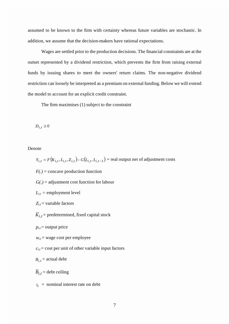
The firm maximises (1) subject to the constraint
0, ≥tiD
Denote
( ) ( )1,,,,,, ,,, −−= titititititi LLGZLKFY = real output net of adjustment costs
F(.) = concave production function
G(.) = adjustment cost function for labour
Li,t = employment level
Zi,t = variable factors
tiK , = predetermined, fixed capital stock
pi,t = output price
wi,t = wage cost per employee
ci,t = cost per unit of other variable input factors
tiB , = actual debt
tiB , = debt ceiling
ti = nominal interest rate on debt

8
With dividend defined as in the curly bracket in (2), the firm’s optimising behaviour is found
as the solution the following dynamic programming problem:
( ) ( ) ( ) ( )[ ] ( ){ }
( )
+
+
+−+−−−=
+
−−−−
titit
t
tittititititititititititiZL
titi
LVr
E
BiBZcLwLLGZLKFYpmaxLVtiti
,,1
1,,.,,1,,,,,,,,
1,1,
11
1,,,,, (2)
For the variable input factors, Zi,t , the first order condition is given by
ti
titi
ti
ti
pc
Z
Y
,
,,
,
, µ∂∂
= (3)
where
Dti
ti
,
, 11
1
ε
µ−
= is the markup and ti
ti
ti
tiDti Y
p
p
Y
,
,
,
,, ∂
∂ε −= is the price elasticity of demand
facing firm i in period t. To see the generality of the formulation, and relating it to other
studies of markup cyclicality, e.g. Domowitz, Hubbard and Petersen (1987), we rewrite (3) as
titi
ti
ij ti
tj
Dt
titi c
Z
Y
Y
Yap ,
,
,
,
,,, 11 =
∂∂
+− ∑≠ ∂
∂ε
(3’)
where Dtε denotes the price elasticity for the industry in period t, ai,t is the ith firm’s market
share, and ti
tj
Y
Y
,
,
∂∂
is the conjectural variation. If there were only one firm, ai,t = 1, and
0,
, =∂∂
ti
tj
Y
Y. Then we get the standard markup pricing expression given in equation (3).

9
Another extreme case is 0, →tia , which yields a competitive market solution. A Cournot
solution emerges when the conjectural variations are set equal to zero. Thus, our formulation
can accommodate several different price games. Note that our measure of markup is related
to the demand elasticity. In equilibrium the markup level and its fluctuations can be explained
by cost changes as well as the product market behaviour of the firm. The estimated markup
will indicate whether an imperfectly competitive market is present.
The first order condition for labour is:
titi
ti
ti
ti
t
tit
ti
ti
ti
ti wL
Yp
rE
L
Yp,
,
1,
1,
1,
1
1,
,
,
,
,
1
1=
+Λ−
+ +
+
+
+
+∂
∂µ∂
∂µ
(4)
where D
ti
Dti
ti,
1,1,
1
11
λ
λ
+
+−=Λ +
+ , and Dti,λ is the Lagrange multiplier associated with the dividend
constraint at time t. If no dividend constraint is binding at times t and t+1, then 01, =Λ +ti ,
and the firm is financially unconstrained. According to equation (4) the present value of a
marginal unit of labour should equal the wage cost wit. The first term at the left hand side,
which equals ti
ti
ti
ti
ti
ti
L
G
L
F
L
Y
,
,
,
,
,
,
∂∂
∂∂
∂∂
−= , represents increased revenue net of labour adjustment
costs. Employment adjustments affect the following period as well. The last term in the
square brackets,
−= ++
ti
ti
ti
ti
L
G
L
Y
,
1,
,
1,
∂∂
∂∂ , represents the cost of postponing employment
adjustment.6 Using the laws of variance on the expectations expression Et[.] and the rational
expectation property, the first order condition for labour may be written as
6 If the firm has to take into account explicit credit limits, financially constrained firms, (for which ( ) ( ) 1,1/1,1 >+++ titi λλ ,) behave as if they face a higher discount rate. This is further addressed below.

10
titi
ti
ti
ti
t
tiIIti
ti
ti
ti
tiIti
t
ti
ti
ti
ti
ti wL
Yp
re
L
Ype
rL
Yp,
,
1,
1,
1,
1
1,1,
,
1,
1,
1,1,
1
1,
,
,
,
, ,1
1cov
1
1=
+Λ−
+
+⋅
+
+Λ−
+ +
+
+
+
++
+
+
++
+
+∂
∂µ∂
∂µ∂
∂µ
(5)
We have replaced the expectation operators with white noise expectation errors, Itie 1, + and
IItie 1, + respectively, which are uncorrelated with any information at time t.
The standard adjustment cost function for labour, introduced by Holt et al. (1960), is
quadratic in employment changes. Since the size of the labour stock in different plants may
vary considerably, we normalise squared employment changes by firm employment level.
The labour adjustment cost function is thus written as
ti
titi L
XsG
,
2,
, 2= (6)
where 1,,, −−= tititi LLX .7 We use a modified version of (6) reading
( ) ( )
≥−⋅
⋅
−+−⋅
+
= −+
−
+
−
otherwise 0
0 if 12 ,1,
2
1,
,2
1,
, aXLDaL
XDa
L
Xs
G titiitti
tiit
ti
ti
it (7)
where +itD is equal to one if Xit is positive and zero otherwise.8 The parameter a is introduced
to capture an assumption that small changes in employment may be associated with small or
7 Including in X some voluntary quitting which does not induce costs, Nickell (1986), will not affect the results. 8 The s-parameter may also be made dependent on the sign of the employment change. However, deriving asymmetric adjustment costs goes beyond the scope of this paper.
11
negligible costs. Thus, we may ignore costs from small adjustments of the labour stock. A
justification for this is that it is hard from existing literature to establish the costs of small
labour adjustments. With a > 0, relative changes in employment must exceed a to be
considered as costly and thus economically interesting.9 When concentrating on costs of
larger employment adjustments only, we therefore introduce the parameter a as a bliss point.
However, in the empirical analyses we will also use the more standard formulation of the
adjustments cost function with a = 0.
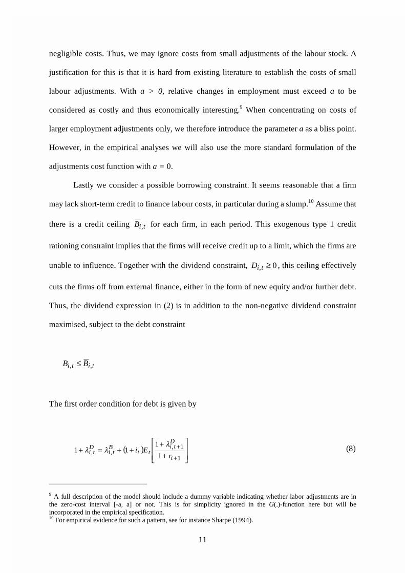
Lastly we consider a possible borrowing constraint. It seems reasonable that a firm
may lack short-term credit to finance labour costs, in particular during a slump.10 Assume that
there is a credit ceiling tiB , for each firm, in each period. This exogenous type 1 credit
rationing constraint implies that the firms will receive credit up to a limit, which the firms are
unable to influence. Together with the dividend constraint, 0, ≥tiD , this ceiling effectively
cuts the firms off from external finance, either in the form of new equity and/or further debt.
Thus, the dividend expression in (2) is in addition to the non-negative dividend constraint
maximised, subject to the debt constraint
titi BB ,, ≤
The first order condition for debt is given by
( )
++
++=++
+
1
1,,, 1
111
t
Dti
ttB
tiD
ti rEi
λλλ (8)
9 A full description of the model should include a dummy variable indicating whether labor adjustments are in the zero-cost interval [-a, a] or not. This is for simplicity ignored in the G(.)-function here but will be incorporated in the empirical specification. 10 For empirical evidence for such a pattern, see for instance Sharpe (1994).

12
Here Bti,λ is the shadow value of relaxing the debt ceiling. If 0, =B
tiλ , the first order condition
for debt states that the value of issuing a marginal unit of new debt to finance dividend
payment must equate the discounted value of repaying debt with interests. If the debt
constraint binds, there is a wedge between the residual profit, or dividend, for the current
period and the dividend expected to be paid next period. Defining D
ti
BtiB
ti,
,,
1
~
λ
λλ
+= , the first
order condition for debt, (8), can be rewritten as
+Λ−
=
+−
+
+
1
1,,
1
1
1
~1
t
tit
t
Bti
rE
i
λ (9)
The dividend and borrowing constraints makes it more expensive to transfer resources
between periods, thus having similar effects as an increase in marginal costs compared to an
unconstrained regime, as shown in expression (9).
Now, to arrive at a final expression summarising the optimising behaviour of the firm,
assume that the short term returns to scale in production,
( ) ( )1,,,,,, ,,, −−= titititititi LLGZLKFY , is given by the constant parameter ti,~ν . From
Euler’s theorem, and using the first order conditions (3), (5) and (9), together with the
formulation of adjustment costs in (7), after some rearranging we obtain the following
equation which serves as the basis for our empirical specification:

13
( )
( )
( )( ) 1,
,,
,
,
,
,,
,
,
,
,11,
1,1
1,
1,
1,
1,
,,
1,1,
,1,
,
11,
1,1
1,
1,
1,
1,
,,
1,1,
,1,
,
,
,
,
,
,
,
,,
,,
,
,,
,,
,,
,,
,
,
,,
,,
~.cov~
~111
1~
111
1~
11~
~
+
++
+
+++
+
+
+
+++
+
++
+
+++
+
+
+
+++
+
++
+−
⋅
⋅
−+−⋅
+⋅
−
+
+
⋅
−+−⋅
+⋅
−
+
−
⋅
−+−⋅
+
−+
+=
tititi
ti
ti
ti
titi
ti
ti
ti
Btiit
ti
tiit
ti
ti
ti
ti
titi
titi
ttiti
ti
itti
tiit
ti
ti
ti
ti
titi
titi
ttiti
ti
itti
tiit
ti
ti
ti
ti
titi
titi
ti
titi
titi
titi
titi
ti
ti
titi
titi
eKq
L
Kq
L
DaL
XDa
L
X
L
X
Kq
Lp
i
s
DaL
XDa
L
X
L
X
Kq
Lp
i
s
DaL
XDa
L
X
L
X
Kq
Lps
Kq
Zc
Kq
Lw
Kq
Yp
νµ
νµ
λνµ
µ
νµµ
ν
νµ
(10)
It is reasonable to assume that financial constraints are more severe during a
downturn, leading to higher marginal costs in such periods. Still, the effect from financial
constraints and labour adjustment costs on markups cannot be stated unambiguously. Price
setting and the aggressiveness of firms in their pricing behaviour may also vary over the
business cycle. The concept of super-game perfectness explains how firms through tacit
collusion will be able to charge a market price higher than the price given from a competitive
equilibrium. A tacit collusion exists because of the threat of punishment from the competitors
in later periods if a firm undercuts the collusion price in a given period. Such co-operation
may break down in downturns, Green and Porter (1984), or in booming periods, Rotemberg
and Saloner (1986). We have not modelled explicitly such price games, since we have no
reasons to believe them to be systematic over several industry sectors. However, if tacit or
open co-operation is withheld over the business cycle, then with our modelling set-up,
countercyclical costs will give rise to a procyclical markup. We note also that if demand is
iso-elastic and marginal costs are constant, a constant markup will result.

14
Since prices and marginal costs cannot be directly observed, we follow the strategy of
using the above representation for estimating the markup. The markup will be parameterised
to take into consideration its variation over the business cycle, controlling for the possible
appearance of adjustment costs and financial constraints.
3. Empirical Specification
Several assumptions have to be made in order to estimate the model in equation (10). Firstly,
there may be cyclical fluctuations in markups due to cyclical variation in demand and
marginal costs, which may affect prices and price strategies. Secondly, we have to find a
representation of the unobservable credit constraint multiplier, which according to (10)
affects the optimising behaviour.
We represent the cyclicality of the markup by parameterising ti,µ as
tti Ψ+= 10, µµµ (11)
According to (11), the markup term consists of a constant term, 0µ , and a variable term, 1µ .
The variation is related to changes in gross domestic products tΨ , as measured relative to the
four surrounding years. The tΨ variable is expressed as
( ) ( ) ( ) ( ) ( )( )2112 lnlnlnln4
1ln ++−− +++−=Ψ tttttt GDPGDPGDPGDPGDP (12)

15
The variable tΨ picks up the degree to which demand each year is higher or lower than the
general trend. We will use a Taylor approximation of first order for the term 1,
,
+ti
ti
µµ in (10).
We have tried several ways to represent a firm’s potential financial constraint. Interest
payments as a share of cash flow seem to represent the data at best (see also Whited (1992),
and Hubbard, Kashyap, and Whited (1995) for related discussion and alternative
formulations). Thus, it is those firms which pay the highest interest rates in relation to its per
period cash flow, which are most likely to be rationed. This interest payment ratio may be
interpreted as serving as a signal of the firm's bankruptcy risk. When paying a high interest
rate, as measured by interest payments to cash flow, a firm is assumed to be less capable of
serving additional debt. Alternatively, such a firm will have to pay a high premium if it is to
obtain further debt finance. Thus, we parameterise the debt multiplier Bti,
~λ as
ti
tiBti
CF
IE
,
,,
~ αλ = (13)
where IEi,t is the interest expenditure and CFi,t is cash flow in period t. Both variables are
measured at firm level, i.e. they are an aggregate over all plants within a firm. Even though
we use plant level data when estimating markup, we assume that it is the financial position of
the parent firm that is most relevant for considering a plant's financial situation. It is at the
firm level that the formal accounting information to be used by external sources is reported.
Furthermore, a plant belonging to a larger firm must be assumed to be able some way or other
to participate in the common value of all the merged plants.
The final model to be estimated is given by (10), with the expressions (11)-(13)
substituted for ti,µ and Bti,
~λ . When estimating the model in (10), we will include a firm

16
specific fixed effect. The fixed firm effect can be interpreted as accounting for firm specific
characteristics that are constant over the sample period. We have also included time dummies
to represent the effect of macro shocks. The estimation is carried through separately for each
sector, since we want to allow for sectoral differences in the parameters.
We assume that the decision-makers have rational expectations, i.e. the errors they
make in forecasting are uncorrelated with the information available when the forecasts are
made. This rational expectations hypothesis suggests orthogonality conditions that can be
used in a generalised method of moments (GMM) as outlined in Hansen (1982). Variables
dated t and earlier which are correlated with the variables in the regression, are valid
instruments given that the error term, ei,t+1, is serially uncorrelated. The firm-fixed effects are
removed by estimating the model in first-differences and, therefore, a first-order serial
correlation is introduced. We apply the m2 test to control for the absence of higher order
serial correlation. Further testing for the validity of the instruments is done by the
Sargan/Hansen test.11 In our estimation, we have used the following variables in levels as
instruments, ii
i
ii
iiii LCF
IE
CF
IEL
Kq
X
Kq
ZcLw i
i
ii
ii
⋅+ , , , , , all at dates t-1 and earlier.
The GMM-estimates of the model expressed in equation (10) give unrestricted
estimates of the deep parameters of interest; 0µ , 1µ , ν~ , s, and α . To find these latter
parameters from the GMM-estimates we use a minimum distance estimation method.12. We
restrict the s parameter in the adjustment function to be non-negative by assuming )exp(η=s
and allowing � to be computed without restrictions. We have also restricted the . parameter
11 See Arellano and Bond (1991) for a complete discussion of both the m2-test and the overidentification test. 12 The proof of the consistency and asymptotic normality of the minimum distance estimator can be found in appendix 3A, Hsiao (1986).

17
in (13) to be within a reasonable interval by assuming )exp(1
)exp(
ξξκα
+= , where � can take any
value and � is the upper limit of ..
4. Data.
The empirical analysis is carried through at the plant level. Variables representing financial
constraints are constructed from the balance sheet of the firm to which the plant belongs.13
The empirical work is based on a large set of unbalanced data of Norwegian plants
and firms within manufacturing industry for the period 1978-1991. The data are collected by
Statistics Norway. Income statement and balance sheet information are provided from
Statistics of Accounts for all firms with more than 50 employees during the period 1978-
1990. There may still be firms of smaller size in the sample. The reason is that information is
collected once the firm is registered. In 1991 no new small firms (less than 100 employees)
were added to the sample due to new sampling routines used by Statistics Norway. For all
firms included in Statistics Norway’s Statistics of Accounts, plant level information about
production, production costs, investment and capital stock is available from the
Manufacturing Statistics. All data are annual. The micro level data are matched with
information about the gross domestic product at sector level. The industry sector values are
collected from National Accounts.
We investigate plants where the changes in the number of employees are of
reasonable magnitude. Observations with employment level 3 times larger than or less than
1/3 of the employment previous year, are therefore excluded. Furthermore, to make the
13 See the Data Appendix for details on variable definitions and construction.

18
sample as homogeneous as possible, we include only plants with more than 5 and fewer than
500 employees, whereas firm size is limited to 1500 employees. Lastly we exclude
observations where the calculated annual man-hours worked per employee are outside the
interval [400,2500].
As discussed in Section 2, we assume that small changes in employment may be
associated with small or negligible costs. We therefore use two different formulations of the
adjustments costs, with a = 0 and a = 0.05. With the latter formulation, the employment
adjustment costs are zero when 05.0<
− a
L
X
it
it .
The descriptive statistics are reported in Table 1. We see that the sales/capital ratio,
pY/qK, as well as the costs/capital ratio, (wL+cZ)/qK, vary among the industries. Comparing
the differences between the sales/capital ratio and the costs/capital ratio, we find that these
differences are approximately 0.1, which indicates the presence of a markup and possibly
some degree of market power. Size differences between and within industries are noticeable.
As measured by average number of employees per firm it varies from 78 to 183. The average
firm size is over 100 employees in most industries, which in a Norwegian context implies that
we are dealing with relatively large plants. This may have implications for our latter findings
about adjustment costs and financial constraints. Although not reported in Table 1, it should
be noted that the minimum plant size is 5 and the largest is 491. Details about labour
adjustments are reported in the same table. The frequencies of labour stock increases seem to
be somewhat higher than the frequencies of reductions in the labour stock. At the same time
we find the average labour adjustment to be just below zero. We see that the frequencies of
labour adjustments in the interval a (=∆L/L) ∈ (-0.05,0.05) are around 40-45 percent.

19
5. Results
The estimation results are reported in Tables 2-5, for different formulations of adjustment
costs and the financial constraint multiplier.
The null hypothesis is no market power, implying a base markup 10 ≈µ . The cyclical
part of the markup, 1µ , may be positive or negative, indicating pro- and countercyclical
markup fluctuations respectively. To interpret its size and magnitude, assume that we find
5.01 =µ . This implies that a relative change in the (detrended) GDP of 6 percent increases
the markup by 0.03, for instance from 1.00 to 1.03. With the restriction on labour adjustment
costs, we will get an adjustment cost parameter s ≥ 0, and similarly for the parameter
associated with the financial constraint, 0≥α . We assume constant unit elasticity of scale.
This assumption is supported by the findings in Klette (1999) that increasing returns to scale
are not a widespread phenomenon in Norwegian manufacturing industries.
We report only the restricted estimates revealed by the minimum distance procedure.
The unrestricted parameter estimates of the Euler equation used for calculating the deep
parameters are at the outset (Table 2) based on first step estimates of GMM, denoted GMM1,
which makes use of a consistent but suboptimal weighting matrix. In Tables 3-5 we report
second step estimates of the deep parameters, GMM2, with an optimal weighting matrix.
In Table 2 we use what may be termed the standard adjustment cost function, i.e. a =
0. The financial constraint multiplier . is restricted to be non-negative but with no upper
bound. The results are based on unrestricted GMM1 results. We find that the invariant
markup term, µ0, deviates significantly from unity in two out of eight industries. An estimate
of µ0 ≥ 1 is consistent with the descriptive statistics in Table 1, and also with other
international studies using an Euler-equation approach on panel data (see for instance Whited

20
(1992) and Hubbard et al. (1995)). For industries with a fixed markup term statistically
insignificant from one, we should not rule out that some degree of market power is relevant
even though it does not follow directly from the results in Table 2. For instance, some
fluctuations in the markup may indicate periods where market power is effective, but the
potential to reap these benefits are not present continuously, due to price setting procedures
(‘price wars’) as well as cost fluctuations. It is also worth noting that a richer set of
instruments, and the utilisation of more orthogonality conditions in GMM, might produce
sharper estimates. However, we are restricted in this sense since the relatively small number
of firms in each of the sectors limits our set of instruments. We note therefore that Klette
(1999) finds small but statistically significant market power (µ0 greater than one) when using
larger panel data sets of Norwegian manufacturing industry.
The cyclical markup term is statistically different from zero in three out of the eight
sectors. For Textiles (321-4) and Mineral Products (361-9) there is evidence of
countercyclical markups, while for Wood Products and Furniture (331-2) there is a
significant procyclical markup. For the other sectors there are non-significant procyclical
fluctuations in markups. The generally (weak) tendency of procyclical markups corresponds
to the findings of Domowitz, Hubbard and Petersen (1986, 1987), Chirinko and Fazzari
(1994) and Bottasso, Galeotti and Sembenelli (1997). However, the difference in the signs of
the cyclical markup-terms among sectors gives support to what is stressed in the “new
industrial organisation literature”, namely that, when investigating industry behavior, the
preferred unit of study should be industries defined as narrow and homogeneous as possible
This includes the analysis of price setting and markups.
According to (10), adjustment costs for labour will affect the marginal costs and the
pricing behaviour of firms. The employment adjustment costs parameter, s, is statistically
different from zero only for Food (311). Thus, it seems like labour adjustment costs do not

21
play an important role for the industry sectors in question. It should be noted that the
insignificant adjustment costs parameter may only be used to reject the symmetric and
convex adjustment costs structure, not to exclude the existence of labour adjustment costs in
general. We have also tried specifications with different formulations, including asymmetric
adjustment costs, without this giving sharper results, and we will see below that the
introduction of a zero cost interval will not dramatically change the result that labour
adjustment costs may play a negligible role. We note that several other studies tend to find
relatively small adjustment costs for labour, see Hamermesh and Pfann (1996). The
insignificance of the labour adjustment costs coefficient here may be explained by particular
Norwegian institutional arrangements during the period of investigation, when it was actually
relatively easy for firms to lay off workers temporarily. During short-term unemployment
spells, the workers could claim unemployment compensation that was not far below their
ordinary wage rates. These rules have now been somewhat changed, which may affect labour
adjustment costs were these to be estimated on more recent data.
The frequent insignificance of a binding capital constraint may be related to the
negligible adjustment costs, although our formulation would be able to represent other
reasons for capital shortage. The coefficient is significant for Food (311) only. Moreover, for
this sector the labour adjustment cost parameter is significant. We have experimented with
several different formulations of the capital constraint but no other formulation commonly
used in the literature gives better or sharper estimates of the shadow price of capital, or on the
adjusted discount factor of the firms. Some of the reported values are too high, indicating that
its interval of variation should be restricted. To see this, note that with the given
parameterising of Bti,
~λ , α measures the change in discount factor when the interest payments
increase relative to the cash flow, holding the investment opportunities constant. The average
discount factor in the sample is 0.95. Thus, an estimate of the interest-cash flow ratio

22
coefficient of 5.0, together with an increase in the interest-cash flow ratio from 0.11 to 0.12 (a
9 percent increase) will decrease the discount factor with 0.04. Even this reduction is rather
large, and estimates of a > 5 will give quite dramatic changes in discount factors compared to
the estimates reported in e.g. Hubbard and Kashyap (1992) and Hubbard et al. (1995). Such
estimates should thus indicate that the capital market restrictions would seriously influence
the intertemporal behaviour of a firm.
Our estimated results are only valid as long as the overidentification test does not
reject the chosen set of instruments, and when there is no serial correlation in the error terms.
In Table 2, the Sargan test rejects the set of instruments for Wood Products and Furniture
(331-332) and Paper Products (341). In the same table, both the overidentifaction test and the
m2-test reject the set of instruments for Metals (371-372). This is also the case when lagging
the instruments t-3 but for sake of brevity these latter results are not reported.
In Table 3 we report the same set of results for the deep parameters based on GMM2
unrestricted estimates. Note, however, that the second step of the two-step GMM procedure
appears to overstate the efficiency gains, see Arrelano and Bond (1991). With this in mind,
we point out that neither the m2 test nor the Sargan test reject our set of instruments for any
of the analysed industries. If we concentrate on the parameters of interest, the overall picture
is that several fixed and cyclical markup terms are now statistically significant. There is no
change of sign compared to results in Table 2 but we now find a statistically significant
procyclical markup in all sectors except for Textiles (321-4) and Mineral Products (361-9).
Moreover, according to Table 2 markup fluctuations were countercyclical for these two
sectors. Contrary to the results reported in Table 2, we find that the labour adjustment cost
parameter s is zero for five out of the eight analysed industries and still significant only for
Food (311). This is not necessarily an unreasonable result, and we note that the capital

23
FRQVWUDLQWV� DV PHDVXUHG E\ .� DUH VWLOO VLJQLILFDQW RQO\ ZKHQ ODERXU DGMXVWPHQW FRVWV DUH
present (sector 311).
To check the robustness of these estimates, we report in Table 4 the results when
assuming that small adjustments of employment do not carry any costs. As described by the
summary statistics, a large fraction of labour adjustments takes place in the interval a
(=∆L/L) ∈ (-0.05,0.05), which might indicate zero or very small adjustment costs for an
interval around zero. Thus, we set a = 0.05 in the adjustment costs function (the G(.)-
function). The results in Table 4 should be compared to the estimates reported in Table 3, as
they are all based on GMM2 results. There is little change in results other than for two
sectors, Chemicals (351-6) and Metals (371-2). These two sectors show insignificant
procyclical markup fluctuations. Magnitude and significance of labour adjustment costs and
shadow price of capital remain the same.
Lastly, in Table 5 we restrict the capital market coefficient, .� WR EH OHVV WKDQ �. With
an interest expenditure to cash flow ratio equal to 0.2, which is in the 90% percentile of the
interest cash-flow ratio, and α=5.0, then Bti,
~λ = 1.0, and thus a discount factor equal 0. Lower
levels of α produces higher discount factors. We see that markup levels and its cyclicality
remain basically unaltered over industries compared to the results reported in Table 4. For
labour adjustment costs there is one change. The coefficient s is now significant also for
Textiles (321-4), and even the capital market coefficient α becomes significant for this sector.
6. Concluding remarks
We have used a structural approach to estimate markup and its fluctuations over the business
cycle for a panel of Norwegian manufacturing firms. An advantage of this method, which

24
draws on the research strategy of the ‘new empirical industrial organisation’ is that it
economises on information. We avoid collecting data to represent variables that are in reality
unobservable, and can thus study several firms and industries simultaneously.
The general findings are that some market power seems to prevail, and that markups
in Norwegian manufacturing as measured from a sample of medium sized firms seem to vary
procyclically for most manufacturing industry sectors. However, there are also sectors with
countercyclical markup behaviour. Labour adjustments costs seem not be of large importance
but, when they are significant, there is also a tendency for some capital market imperfection
to prevail.
Some caveats and suggestions for extensions are in place. Firstly, care should be taken
when in general interpreting the importance of financial constraints for the variations in
markups. It is well established that capital market imperfections may lead to financial
constraints. However, in the presence of financial constraints, the output prices and the
markups of the liquidity constrained firms may go in either direction. The insignificance of
the financial variable coefficient may be a result of competing effects working
simultaneously. To reveal the simultaneous event of financial constraints, employment
adjustment costs, and markup fluctuations might therefore require even more homogeneous
and narrowly defined sectors than studied here. Another test of the importance of financial
constraints, which might give some insight, would be to split the sample into a priori
financial constrained and non-constrained firms. However, with the limited number of
observations in some of the sectors, it would be difficult to get separate estimates for the two
sub-samples, and there would be too few observations to get reliable GMM-estimates.
Therefore, we did not choose this research path. It may be the case that the insignificance of
the debt constraints is due to sample selection biases. The sample used consists of plants with
at least six consecutive observations belonging to firms with more than 50 employees. These

25
firms are in fact relatively large within the Norwegian manufacturing industry and their
access to credit should therefore be better than for smaller firms.14 The relatively easy access
to credit may also explain why labour adjustment costs are of negligible significance for
forward looking firms over a business cycle. Therefore, it might be the case that financial
constraints are less likely for firms in our sample, and there is no strong evidence from other
Norwegian studies that financial constraints strongly affect firms’ behaviour.
In total, it seems that factor markets and financial constraints will affect markup
behaviour only to a limited degree. Further studies on markup cyclicality should therefore
focus more on price setting behaviour and price games. Such studies would require much
narrower industry groups for defining a relevant product market.
14 Data from the Manufacturing Statistics reveal that approximately 85 percent of all firms have less than 50 employees.

26
References Arellano, M., and S. and Bond, 1991, “Some Tests of Specification for Panel Data: Monte
Carlo Evidence and an Application to Employment Equations”, Review of Economic Studies 58, 277-97.
Bils, M., 1987, “The Cyclical Behavior of Marginal Cost and Price”, American Economic
Review 77, 838-55. Borenstein, S. and A. Shepard, 1996, “Dynamic Pricing in Retail Gasoline Markets”, Rand
Journal of Economics 27, 429-51. Bottasso, A., M. Galeotti and A. Sembenelli, 1997, “The Impact of Financing Constraints on
Markups: Theory and Evidence From Italian Firm Level Data”, Fondazione Eni Enrico Mattei Note di Lavoro: 73/97.
Brander, J.A. and T.R. Lewis, 1986, “Oligopoly and Financial Structure: The Limited
Liability Effect”, American Economic Review 76, 956-70. Brander, J.A. and T.R Lewis, 1988, “Bankruptcy Costs and the Theory of Oligopoly”,
Canadian Journal of Economics 21, 221-43. Chatelain, J.B.,1999, “Taux de marge et structure financiere”, Annales d'Economie et de
Statistique 53, 127-47. Chevalier, J.A., 1995, “Capital Structure and Product-Market Competition: Empirical
Evidence from the Supermarket Industry”, American Economic Review 85, 415-35. Chevalier, J.A., and D.S. Scharfstein, 1995, “Liquidity Constraints and Cyclical Behavior of
Markups”, American Economic Review, Paper and Proceedings 85, 390-6. Chevalier J.A., and D.S. Scharfstein, 1996, “Capital Market Imperfections and
Countercyclical Markups: Theory and Evidence”, American Economic Review 86, 703-25.
Chirinko, R.S., and S.M. Fazzari, 1994, “Economic Fluctuations, Market Power, and Returns
to Scale: Evidence from Firm-Level Data”, Journal of Applied Econometrics 9, 47-69. Domowitz, I., R.G. Hubbard, and B.C. Petersen, 1986, “Business Cycles and the Relationship
between Concentration and Price-Cost Margins”, Rand Journal of Economics 17, 1-17.
Domowitz, I., R.G. Hubbard, and B.C. Petersen, 1987, “Oligopoly Supergames: Some
Empirical Evidence on Prices and Margins”, Journal of Industrial Economics 36, 9-28.
Galeotti M., and F. Schiantarelli, 1998, “The Cyclicality of Markups in a Model with
Adjustment Costs: Econometric for U.S. Industry”, Oxford Bulletin of Economics and Statistics 60, 121-42.

27
Gottfries, N., 1991, “Customer Markets, Credit Market Imperfections and Real Price Rigidity”, Economica 58, 317-23.
Green E., and R. Porter, 1984, “Noncooperative Collusion under Imperfect Price
Information”, Econometrica 52, 87-100. Hamermesh, D.S., and G.A. Pfann, 1996, “Adjustment Costs in Factor Demand”, Journal of
Economic Literature 34, 1264-92. Hansen, L.P., 1982, “Large Sample Properties of Generalized Method of Moments
Estimators”, Econometrica 50, 1029-54. Hendel, I., 1996, “Competition under Financial Distress”, Journal of Industrial Economics
44, 309-24. Hendel, I., 1997, “Aggressive Pricing as a Source of Funding”, Economics Letters 57, 275-
81. Holt, C., F. Modigliani, J. Muth and H. Simon, 1960, “Planning Production Inventories, and
Work Force”, Prentice Hall. Hsiao C., 1986, “Analysis of panel data”, Econometric Society Monographs no. 11,
Cambridge; New York and Sydney: Cambridge Hubbard, R.G., 1998, “Capital-Market Imperfections and Investment”, Journal of Economic
Literature 36, 193-225. Hubbard, R.G. and A.K Kashyap, 1992, “Internal Net Worth and the Investment Process: An
Application to U.S. Agriculture”, Journal of Political Economy 100, 506-34. Hubbard, R.G., A.K Kashyap, and T.M. Whited, 1995, “International Finance and Firm
Investment”, Journal of Money, Credit, and Banking 27, 683-701. Klette, T.J., 1999, “Market Power, Scale Economies and Productivity: Estimates from a Panel
of Establishment Data”, Journal of Industrial Economics 47, 451-76. Maksimovic, V. 1988, “Capital Structure in Repeated Oligopolies”, Rand Journal of
Economics 19, 389-407. Nickell, S., 1986, “Dynamic Models of Labour Demand”, ch. 9 in Handbook of Labor
Economics I, ed. by O. Ashenhelter and R. Layard, Elsevier Science Publishers. Nilsen, Ø.A. and F. Schiantarelli, 1998, “Zeroes and Lumps: Investment Patterns of
Norwegian Firms”, Working Paper No. 337, Department of Economics, Boston College.
Phillips, 1995, “Increased Debt and Industry Product Markets: An Empirical Analysis”,
Journal of Financial Economics 37, 189-238.

28
Rotemberg J.J., and G. Saloner, 1986, “A Super Game Theoretic Model of Price Wars during Booms”, American Economic Review 77, 390-407.
Sharpe, S.A., 1994, “Financial Market Imperfections, Firm Leverage, and the Cyclicality of
Employment”, American Economic Review 84, 1060-74. Showalter, D.M., 1995, “Oligopoly and Financial Structure: Comment”, American Economic
Review 85, 647-53. Stenbacka, R. 1994, “Financial Structure and Tacit Collusion with Repeated Oligopoly
Competition”, Journal of Economic Behavior and Organization 25, 281-92. Whited, T.M., 1992, “Debt, Liquidity Constraints, and Corporate Investment: Evidence from
Panel Data”, Journal of Finance 47, 1425-60.
29
DATA APPENDIX 1. Criteria for Sample Selection Firms in which the central or local governments own more than 50 percent of the equity have been excluded from the sample, as well as observations that are reported as “copied from previous year”. This actually means missing data. We also excluded observations from auxiliary (non-production) plants as well as plants where part-time employees count for more than 25 percent of the work force. Since the capital stock is used as the denominator in most of the variables used in the regression analysis, we make an attempt to isolate plants whose capital stock has a negligible role in production. Observations where the calculated replacement value of equipment and buildings together was less than NOK 200,000 (1980 prices) are deleted.15 To avoid measurement errors of production, observations with non-positive production levels are also deleted. The remaining data set was trimmed to remove outlayers. Observations with ratios outside of five times the interquartile range above or below the sector specific median were excluded.16
Our analysis is conducted on plants belonging to the manufacturing industry sectors (ISIC code in parentheses): Food (311), Textiles and Clothing (321-324), Wood Products (331-332), Paper and Paper Products (341), Chemicals (351-356), Mineral Products (361-369), Metals (371-372), Metal Products and Machinery (381-382). Some of the plants changed sector during the sample period. We group these plants into the sector where they had their highest frequency of observations.
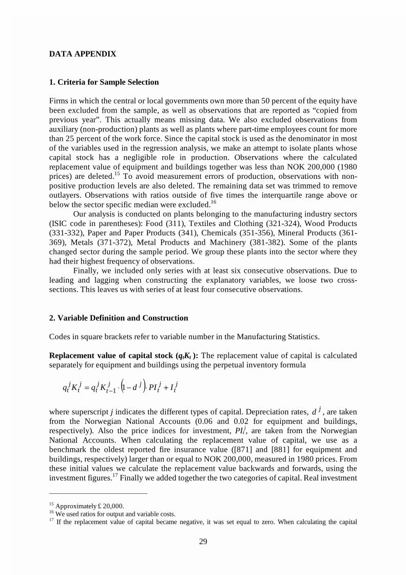
Finally, we included only series with at least six consecutive observations. Due to leading and lagging when constructing the explanatory variables, we loose two cross-sections. This leaves us with series of at least four consecutive observations. 2. Variable Definition and Construction Codes in square brackets refer to variable number in the Manufacturing Statistics. Replacement value of capital stock (qtKt ): The replacement value of capital is calculated separately for equipment and buildings using the perpetual inventory formula
( ) jt
jt
jjt
jt
jt
jt IPIdKqKq +⋅−⋅= − 11
where superscript j indicates the different types of capital. Depreciation rates, jd , are taken from the Norwegian National Accounts (0.06 and 0.02 for equipment and buildings, respectively). Also the price indices for investment, PIt
j, are taken from the Norwegian National Accounts. When calculating the replacement value of capital, we use as a benchmark the oldest reported fire insurance value ([871] and [881] for equipment and buildings, respectively) larger than or equal to NOK 200,000, measured in 1980 prices. From these initial values we calculate the replacement value backwards and forwards, using the investment figures.17 Finally we added together the two categories of capital. Real investment
15 Approximately £ 20,000. 16 We used ratios for output and variable costs. 17 If the replacement value of capital became negative, it was set equal to zero. When calculating the capital

30
at time t in capital of type j equals purchases minus sales of fixed capital. Investments in equipment include machinery, office furniture, fittings and fixtures, and other transport equipment, excluding cars and trucks ([501]+[521]+[531]-[641]-[661]-[671]). The measure of buildings includes buildings used for production, offices and inventory storage ([561]-[601]). Output (ptYt): Gross production [1041], plus subsidies [291], and minus taxes [301]. Variable costs: (wtLt + ctZt): Wage expenses [291] and inputs [1061]. Employees (Lt ): Number of employees [131]. The change in the labor stock is defined as
1−−= ititit LLX . We have assumed that small relative employment changes,
05.0<
− a
L
X
it
it , are zero.
Interest Expenditure (IR/CF): Profit before year-end adjustments [310]Accounts normalised with the cash-flow defined as the sum of Operating Profit [2400]Accounts, Depreciation [2290]Accounts, and Wage Expences [2120+2140]Accounts. Real interest rates (it): We have used interest rates for loans with three months duration (NIBOR) minus the Consumer Price Index. Price indices (pt): Price indices for industry sectors gross output collected from National Accounts. Gross Domestic Product (GDPt): The industry sector values are collected from National Accounts. The GDPt values are annual. For sectors where the National Accounts give information at a less aggregated level than our sector specification, we have used the more detailed information.
stock forward it may happen that the replacement value becomes negative because of large sales of capital goods. When calculating it backwards the replacement value becomes negative if the net purchase of fixed capital is larger than the replacement value in year t+1.

30
Ta
ble
1.
Su
mm
ary
sta
tis
tic
s Fo
od
Te
xti
les
an
dW
oo
dP
ap
er
Ch
em
ica
lsM
ine
ral
Me
tals
Me
tal
Pro
du
cts
Clo
thin
gP
rod
uc
tsP
rod
uc
tsa
nd
Ma
ch
ine
ryS
ec
tors
(31
1)
(32
1-3
24
)(3
31
-33
2)
(34
1)
(35
1-3
56
)(3
61
-36
9)
(37
1-3
72
)(3
81
-38
2)
pY
/qK
2.2
16
1.4
12
1.4
40
0.9
17
1.3
29
1.1
19
1.1
13
1.5
27
(wL
+c
Z)/
qK
2.1
07
1.3
30
1.3
09
0.8
40
1.1
62
0.9
96
0.9
87
1.4
26
Int.
ex
p/
ca
sh
flo
w0
.10
50
.09
70
.12
30
.10
60
.11
30
.10
90
.14
40
.08
8L
it7
19
18
21
28
91
10
21
75
10
4∆
Lit/
Lit
-0.0
19
-0.0
48
-0.0
16
-0.0
27
-0.0
36
0.0
28
-0.0
08
-0.0
28
Fre
q.
∆ L
it/L
it <
-0
.05
0.3
07
0.3
94
0.2
88
0.2
96
0.3
29
0.3
22
0.2
87
0.3
27
-0
.05
<=
∆ L
it/L
it <
= 0
.05
0.4
41
0.4
15
0.4
41
0.4
88
0.4
35
0.4
45
0.4
47
0.4
23
0
.05
<
∆ L
it/L
it0
.25
20
.19
10
.27
10
.21
50
.23
60
.23
30
.26
70
.25
0
∆
Lit
/Lit
= 0
0.1
79
0.0
91
0.1
25
0.1
04
0.1
03
0.1
21
0.0
47
0.0
91
Nb
r. o
f fi
rms
30
57
11
28
65
10
66
43
01
86
Nb
r. o
f o
bs
erv
atio
ns
21
18
53
01
07
35
37
87
65
44
30
01
49
0

31
Fo
od
Te
xti
les
an
dW
oo
dP
ap
er
Ch
em
ica
lsM
ine
ral
Me
tals
eta
l P
rod
uc
tsS
ec
tor
Clo
thin
gP
rod
uc
tsP
rod
uc
tsa
nd
Ma
ch
ine
ry(3
11
)(3
21
-32
4)
(33
1-3
32
)(3
41
)(3
51
-35
6)
(36
1-3
69
)(3
71
-37
2)
(38
1-3
82
)
µ00
.98
01
.08
4*
1.0
45
1.0
78
*1
.00
91
.06
41
.07
81
.00
2(0
.04
0)
(0.0
30
)(0
.06
3)
(0.0
28
)(0
.08
5)
(0.0
71
)(0
.05
5)
(0.0
47
)
µ10
.03
4-2
.73
0*
0.3
30
*0
.22
70
.15
6-0
.84
7*
0.0
55
0.2
19
(0.0
65
)(0
.06
8)
(0.1
64
)(0
.19
6)
(0.1
04
)(0
.31
4)
(0.1
33
)(0
.14
3)
s3
4.4
98
1.0
93
38
.47
42
.61
30
.00
04
.56
57
.15
12
.04
4(2
0.3
93
)(2
.42
3)
(20
.66
3)
(6.9
48
)(2
4.9
88
)(4
1.0
56
)(2
3.8
51
)(2
.99
1)
α7
.06
34
1.0
36
11
.40
91
3.0
57
3.2
27
0.0
00
28
.71
97
.84
0(3
.87
6)
(70
.36
9)
(7.0
62
)(2
6.4
13
)(1
.7 E
+9
)(1
08
.45
0)
(71
.77
6)
(47
.98
6)
m2
-te
st-1
.90
0.1
2-0
.62
-0.7
8-1
.73
1.6
3-1
.90
-0.7
0
p-v
alu
e0
.06
0.9
10
.53
0.4
40
.08
0.1
00
.06
0.4
9
Sa
rga
n
35
.28
37
.13
16
9.6
77
9.5
14
6.3
14
3.2
47
3.4
66
1.0
5
p-v
alu
e0
.82
0.7
60
.00
0.0
00
.38
0.5
00
.00
0.0
5
Inst
rum
en
ts u
sed
:t-
2t-
2t-
1,
t-2
t-2
t-2
t-2
t-2
t-2
Nb
r. o
f fir
ms
30
57
11
28
65
10
66
43
01
86
*
Ind
ica
tes
sig
nifi
can
ce a
t th
e
5 %
leve
l.
1)
De
pe
nd
en
t va
ria
ble
is p
Y.
All
vari
ab
les
are
no
rma
lise
d w
ith q
K2
) F
or
vari
ab
le d
efin
itio
ns,
se
e D
ata
Ap
pe
nd
ix.
3)
All
sta
nd
ard
err
ors
in p
are
nth
ese
s a
re r
ob
ust
to
he
tero
ske
da
stic
ity.
4)
m2
is a
te
st o
f se
con
d o
rde
r se
ria
l co
rre
latio
n.
5)
Sa
rga
n/H
an
sen
is t
he
Sa
rga
n/H
an
sen
te
st o
f o
veri
de
ntif
ica
tion
re
stri
ctio
ns.

32
Fo
od
Te
xti
les
an
dW
oo
dP
ap
er
Ch
em
ica
lsM
ine
ral
Me
tals
eta
l P
rod
uc
tsS
ec
tor
Clo
thin
gP
rod
uc
tsP
rod
uc
tsa
nd
Ma
ch
ine
ry(3
11
)(3
21
-32
4)
(33
1-3
32
)(3
41
)(3
51
-35
6)
(36
1-3
69
)(3
71
-37
2)
(38
1-3
82
)
µ0
1.0
05
1.0
78
*1
.14
0*
1.0
33
*1
.02
11
.14
9*
0.9
93
1.0
42
*(0
.01
6)
(0.0
06
)(0
.00
4)
(0.0
08
)(0
.03
8)
(0.0
25
)(0
.03
3)
(0.0
18
)
µ1
0.0
77
*-0
.25
7*
0.2
69
*0
.47
8*
0.1
16
*-0
.88
3*
0.2
26
*0
.19
3*
(0.0
31
)(0
.01
5)
(0.0
17
)(0
.02
4)
(0.0
40
)(0
.10
2)
(0.0
93
)(0
.05
4)
s1
5.7
91
*0
.23
20
.00
00
.00
00
.00
00
.00
00
.00
00
.44
7(7
.95
7)
(0.8
16
)(0
.84
7)
(1.3
44
)(7
.24
6)
(6.5
00
)(1
6.9
87
)(1
.66
7)
α1
2.9
31
*1
23
.25
71
.88
90
.42
60
.26
32
8.0
15
0.2
03
18
.17
5(5
.81
9)
(42
7.9
43
)(1
.7 E
+8
)(2
.5 E
+1
0)
(1.4
E+
10
)(7
.1 E
+1
1)
(6.3
E+
12
)(1
19
.63
7)
m2
-te
st
-1.9
50
.26
-0.6
4-0
.65
-1.2
61
.66
-1.9
0-0
.78
p
-va
lue
0.0
50
.80
0.5
20
.52
0.2
10
.10
0.0
60
.44
Sa
rga
n
38
.52
43
.60
99
.50
45
.86
45
.33
43
.17
14
.47
55
.19
p
-va
lue
0.7
10
.49
0.3
30
.40
0.4
20
.51
1.0
00
.12
Ins
tru
me
nts
us
ed
:t -
2t-
2t-
1,
t -2
t -2
t -2
t -2
t -2
t -2
Nb
r. o
f fi
rms
30
57
11
28
65
10
66
43
01
86
No
tes
: S
ee
Ta
ble
2.

33
Fo
od
Te
xti
les
an
dW
oo
dP
ap
er
Ch
em
ica
lsM
ine
ral
Me
tals
eta
l P
rod
uc
tsS
ec
tor
Clo
thin
gP
rod
uc
tsP
rod
uc
tsa
nd
Ma
ch
ine
ry(3
11
)(3
21
-32
4)
(33
1-3
32
)(3
41
)(3
51
-35
6)
(36
1-3
69
)(3
71
-37
2)
(38
1-3
82
)
µ0
1.0
05
1.0
78
*1
.09
3*
1.0
08
1.0
37
1.1
77
*1
.07
1*
1.0
36
*(0
.01
7)
(0.0
05
)(0
.02
2)
(0.0
14
)(0
.03
4)
(0.0
27
)(0
.03
1)
(0.0
18
)
µ1
0.0
76
*-0
.27
1*
0.3
19
*0
.41
2*
0.0
06
-0.5
75
*0
.01
20
.17
4*
(0.0
32
)(0
.01
5)
(0.0
50
)(0
.04
8)
(0.0
42
)(0
.08
4)
(0.0
99
)(0
.05
5)
s2
3.6
10
*1
.38
40
.00
00
.00
00
.80
70
.00
00
.00
00
.00
0(1
1.2
38
)(0
.87
8)
(9.9
03
)(4
.23
7)
(8.1
88
)(9
.49
4)
(23
.84
7)
(1.9
28
)
α1
1.0
55
*2
4.3
85
5.5
53
1.5
43
0.0
00
0.5
94
1.4
01
1.0
36
(4.4
83
)(1
5.2
63
)(6
.5 E
+1
1)
(1.8
E+
9)
(14
3.9
68
)(3
.5 E
+1
2)
(1.1
E+
7)
(1.6
E+
10
)
m2
-te
st
-1.9
90
.02
-0.6
6-0
.20
-1.2
01
.74
-2.0
2-0
.79
p
-va
lue
0.0
50
.81
0.5
10
.84
0.2
30
.08
0.0
40
.43
Sa
rga
n
35
.68
45
.96
97
.82
39
.47
44
.53
40
.94
13
.96
56
.55
p
-va
lue
0.8
10
.39
0.3
70
.67
0.4
50
.60
1.0
00
.10
Ins
tru
me
nts
us
ed
:t -
2t-
2t-
1,
t -2
t -2
t -2
t -2
t -2
t -2
Nb
r. o
f fi
rms
30
57
11
28
65
10
66
43
01
86
No
tes
: S
ee
Ta
ble
2.

34
Fo
od
Te
xti
les
an
dW
oo
dP
ap
er
Ch
em
ica
lsM
ine
ral
Me
tals
eta
l P
rod
uc
tsC
loth
ing
Pro
du
cts
Pro
du
cts
an
d M
ac
hin
ery
Se
cto
rs(3
11
)(3
21
-32
4)
(33
1-3
32
)(3
41
)(3
51
-35
6)
(36
1-3
69
)(3
71
-37
2)
(38
1-3
82
)
µ00
.99
81
.06
4*
1.0
93
*1
.00
81
.03
71
.77
7*
1.0
71
*1
.03
6*
(0.0
17
)(0
.00
5)
(0.0
22
)(0
.01
4)
(0.0
34
)(0
.02
7)
(0.0
31
)(0
.01
8)
µ10
.08
4*
-0.2
69
0.3
19
*0
.41
20
.05
8-0
.57
5*
0.0
12
0.1
74
*(0
.03
2)
(0.0
15
)(0
.05
0)
(0.0
48
)(0
.04
2)
(0.0
84
)(0
.09
9)
(0.0
55
)
s2
6.2
86
(*)
3.3
06
*0
.00
00
.00
00
.80
70
.00
00
.00
00
.00
0(1
1.2
38
)(0
.87
7)
(9.9
03
)(4
.23
7)
(8.1
88
)(9
.49
4)
(23
.84
7)
(1.9
28
)
α5
.00
0(*
)5
.00
0*
0.9
66
2.8
72
0.0
00
3.6
59
4.4
37
2.8
26
(2.7
82
)(1
.94
6)
(4.9
E+
11
)(9
.7 E
+8
)(1
43
.96
8)
(1.1
E+
7)
(8.6
E+
9)
(4.0
E+
7)
m2
-te
st-1
.99
0.0
2-0
.66
-0.2
0-1
.20
1.7
4-2
.02
-0.7
9
p-v
alu
e0
.05
0.8
10
.51
0.8
40
.23
0.0
80
.04
0.4
3
Sa
rga
n
35
.68
45
.96
97
.82
39
.47
44
.53
40
.94
13
.96
56
.55
p
-va
lue
0.8
10
.39
0.3
70
.67
0.4
50
.60
1.0
00
.10
Inst
rum
en
ts u
sed
t-2
t-2
t-1
, t-
2t-
2t-
2t-
2t-
2t-
2
Nb
r. o
f fir
ms
30
57
11
28
65
10
66
43
01
86
No
tes:
Th
e r
esu
lts in
th
is t
ab
le is
ba
sed
on
th
e s
am
e s
et
of
un
rest
ric
ted
es
tima
tes
as
in t
he
pre
vio
us
tab
le.
S
ee
als
o n
ote
s in
Ta
ble
2.