the criticality of the european multimodal transportation

The Criticality of the European Multimodal Transportation Network

Multifaceted Investigation of the European Hinterland Transportation Network based

on Its Network Structure

Andreas Yunus 4740521

i

The Criticality of The European Multimodal Transportation Network Multifaceted Investigation of the European Hinterland Transportation Network based

on Its Network Structure

By

Andreas Yunus

In partial fulfilment of the requirement for the degree of

Master of Science In Engineering and Policy Analysis

Faculty of Technology, Policy, and Management Delft University of Technology

To be defended publicly on August 23rd, 2019

Student Number: 4740521 Graduation Committee: Chairperson : Dr S. W. Cunningham Policy Analysis First Supervisor : Dr S. W. Cunningham Policy Analysis Second Supervisor : Dr J.H.R. Ron van Duin Transport and Logistics External Supervisor : Camill Harter Advisor : Amir Ebrahimi Fard An electronic version of this thesis is available at http://repository.tudelft.nl/ Associated codes and notebook are available at https://github.com/andreasyunus/EHTN_Criticality

http://repository.tudelft.nl/

https://github.com/andreasyunus/EHTN_Criticality

ii

[This page intentionally left blank]

iii

Acknowledgements I am extremely grateful to have an opportunity to study at TU Delft, which is one of the best research university in The Netherlands with a full scholarship. Until now, I still do not believe how that extremely precious opportunity can come to me at the right time. In my third year of working in Procter & Gamble, I was looking for a master’s degree that offers a curriculum in decision making and data analytics with specialisation in economics and finance. I was thinking to continue to master’s degree because I wanted to follow my passion to get the skills in data analytics and also expertise in economics and finance. Initially, I was applying for a scholarship to Sweden and KTH in Stockholm but was rejected. Then, the second country, which is my interest is The Netherlands with TU Delft as the first university of choice due to the excellent reputation that TU Delft has. I did not expect much at that time. Long story short, here I am, in the final year of master’s degree, writing my thesis and scheduled to graduate in August 2019. This study is a result of 6 months of the research project at the Delft University of Technology in partial fulfilment of the master’s degree in engineering and Policy Analysis. This study presents the work in the field of transportation and logistics and is meant to be read by researchers, experts, or someone who has an interest in transportation and logistics. This is a study about criticality analysis of European transport network with an emphasis in multimodality of the hinterland transportation network. Furthermore, this research also includes collaboration and community analysis to detect coalition among European ports. I would like to convey my biggest gratitude to Scott Cunningham, who is the chairman and my first supervisor of this thesis project. I am so thankful for him to introduce me to this exciting topic in transportation and logistics, which is a sub-project of Camill Harter from the Erasmus University of Rotterdam. Without Scott’s thoughtful guidance and feedback, I hardly finish this master thesis. Secondly, I would like to convey my gratitude to Ron van Duin, who is my second supervisor. Thank you for your support and advice as always. Moreover, thank you for introducing me to Ellen Naaijkens in light of getting additional information for completing this thesis. Thirdly, I would like to say thank you for Amir Ebrahimi Fard. Thank you for always sharing your valuable insight of network analysis. Fourthly, thank you for Camill Harter for letting me join your project, contributing to your research. Lastly, to the people who mean a lot to me, thank you for mama and papa who always believe in me and let me follow my passion, still support me in my lowest state, and let me dream higher and higher. Thank you for your love, attention, and motivation so I can become a person that I wish for. This thesis is the ending of my master’s journey at TU Delft, but I believe this is a mark for an exciting new beginning.

Andreas Yunus July 2019 Den Haag

iv

Executive Summary A nation’s main port is a crucial component that contributes to the economic development of a country. Moreover, globalisation further increases the importance or influence the port of a country’s development and even regional economic development. However, increasing regionalisation and polarisation that happens in the European region, which widens the inequality in the network. The rising inequality in the network is detrimental to the economic development in the area due to polarization; hence, the economic wealth is not well-distributed across the region. Furthermore, inequality also affects the sensitivity of the network to targeted disruptions due to the significant roles only hold by some influential hubs in the network. The sensitivity and inequality of the network are framed as a criticality in this study. Then, the research question in this study is: How can the criticality of European multimodal transportation network be analytically

assessed by utilising a complex network science method?

There are three knowledge gaps that are the main objective of this study. Firstly, most of the research has done the centrality analysis by ranking the nodes in a single aggregated network. This method will have some information loss due to a single aggregation of the network components will ignore the multilayer information in a multimodal transportation system. Therefore, this study will employ the multilayer method. Secondly, most of the research in multimodal transportation was only focused in the Northwestern region of Europe compared to only 8.75% for general Europe region. This study will contribute to more research since this study will analyse shipping schedules in the entire European area for four years period (2016 to 2019). Thirdly, most of the research that investigated the criticality only consider the network structure (scale-free or distributed) without taking into account the community structure, morphology, development, and efficiency. This study will integrate and take into account that information and analyse it. To answer the main research question and the knowledge gaps. Four kinds of analysis will be performed in this study, such as the versatility analysis, community structure analysis, and quantification of collaboration and connectivity of the container hubs. Those first analyses are the main building blocks for the last analysis, which is the criticality analysis of the network. Versatility analysis will set the direction of the study, which focuses on the most important or central container hubs in the network. The multilayer analysis will be employed in this case to breakdown the network into several layers and rank the multimodal container hubs accordingly. The result of this analysis is the rank of the container hubs by considering the container hub rank in each network layer. This study intends to set the focus of community developments that are formed around the most versatile hubs in the network. Then, the analysis will be continued by community structure analysis. This analysis is focusing on community structure identification. Multilayer infomap algorithm will be performed for community identification around the most versatile container hubs.

v

Several network metrics will be used in this analysis to measure inequality and make a comparison between communities. The network metrics that will be utilized, such as PageRank, strength, and multiplexity (to measure multimodality). Then, the metrics development in four years period (2016 to 2019) will be analysed. Additionally, the spectral bipartivity to measure network efficiency and the redundancy in network connections between hubs are also measured and investigated. The result of this part is to compare the inequality of each community, as stated earlier. The last building block before performing criticality analysis is the quantification of collaboration between hubs by using network point of view. This additional analysis will provide the information of sustainability of the hubs based on the threat from a potential shift from major carriers’ shipments. There is two quantifications that will be performed, which is the connectivity and the cooperation index. Those measurements will be classified into a matrix that provides information about the sustainability of the hubs. The last analysis is the criticality analysis. This part will utilise the result from previous analyses and do a sensitivity analysis by performing targeted disruptions to the most versatile hubs. Then, the network performance will be measured. The network performance is represented by the network diameter as a representation of the coverage, the mean path length as a representation of the degree of integration and coverage, and also the network density which represents the degree of route choices. After that, the drops in network performance will be analyzed, and recommendations can be done from the analysis. There are several recommendations as to the results of this study. Firstly, increasing the redundancy by focusing intra-community will only increase the inequality or Matthew Effect in the network, and the network will not have a good balance across the region. This kind of relationship will also encourage the duality and polarization in the network. Hence, the network will be prone and vulnerable to targeted disruptions, as shown in this study. Then, it is essential to improve the infrastructures and connections development inter-community. This way, the overall network will be less sensitive to targeted disruptions, and the overall network will have a well-distributed multimodal transportation network which leads to well-distributed economic development across the network and make the whole region more competitive. Secondly, from the experience of this research, most of the literature research and data are focusing on the Northwestern region of Europe, which make it relatively less challenging to find information for Northwestern study while it is more challenging to find high quality information for development in Southern European region. Hence, another recommendation is to have a platform that integrates the data from the whole region. This study investigated the criticality based on network structure. However, since there are multiple determinants that influence the robustness and resilience of the network, such as determinants from operational factors, external factors, and also policies at the institutional level. Future research could integrate more determinants and also utilize deep uncertainty analysis in the study. Deep uncertainty analysis can be performed by using MORDM (Multi-Objective Robust Decision Making) or MORO (Multi-Objective Robust Optimization) framework and tools. Additionally, this study stated that there is a trade-off between more hierarchical structure (which benefits the

vi

container hubs) and more distributed structure (which benefits the customers in terms of lower logistical cost). More distributed structure will put more pressure on the hubs since this structure encourages more competition and increase the potential threat due to the shift of shipping schedules (though it encourages innovation at the same time to increase attractiveness of the hubs), while more hierarchical structure will encourage collaboration but also increase the potential for cartel-like relationship due to preferential-based attachment structure (which increase the potential for higher logistical cost). The recommendation for future research based on this identification is to find the optimum index for cooperation and collaboration based on this trade-off.

vii


viii

Table of Contents

Acknowledgements ...............................................................................................................................................iii

Executive Summary...............................................................................................................................................iv

List of Abbreviations .............................................................................................................................................xi

Table of Figures ....................................................................................................................................................xii

Table of Tables.....................................................................................................................................................xiv

Chapter 1: Introduction ..........................................................................................................................................1

1.1. Introduction ............................................................................................................................................1

1.2. A Well-Integrated and Competitive Multimodal Transportation System ................................................3

1.3. Research in Multimodal Freight Transportation.....................................................................................4

1.4. Thesis Structure ....................................................................................................................................6

Chapter 2: Research Definition .............................................................................................................................8

2.1. On Analyzing Vulnerability and Criticality ..............................................................................................8

2.2. On Analyzing Regionalization and Polarization .....................................................................................9

2.3. Research Gaps....................................................................................................................................10

2.4. Main Research Question .....................................................................................................................11

2.5. Sub-research Questions ......................................................................................................................11

2.6. Research Methods ..............................................................................................................................13

2.7. Research Limitations ...........................................................................................................................13

2.8. Research Flow.....................................................................................................................................14

2.9. The goal of this study ..........................................................................................................................16

2.10. Research Deliverables ........................................................................................................................17

Chapter 3: Concepts.............................................................................................................................................18

3.1. Integration of Different Types of Modes in Container Transportations ................................................18

3.2. Hinterland Transportation Modes and Structure..................................................................................19

3.3. Multilayer Structure in Multimodal Freight Transportation ...................................................................20 3.3.1. Definition of Multilayer Network .................................................................................................22 3.3.2. Types of Multilayer Network.......................................................................................................23 3.3.3. The Role of a Hub in Multimodal Freight Transportation System ..............................................25 3.3.4. Measuring Centrality of Multilayer Network ...............................................................................26

3.4. Ranking the Importance of a Node in Multilayer Network ...................................................................27

3.5. Operationalizing Versatility Measurement in Multimodal Freight Transportation ................................29 3.5.1. Degree Versatility.......................................................................................................................29 3.5.2. Eigenvector Versatility ...............................................................................................................30 3.5.3. PageRank Versatility..................................................................................................................31 3.5.4. Katz Versatility ...........................................................................................................................31

3.6. Multimodality and Multiplexity ..............................................................................................................32

3.7. Inequality in The European Multimodal Transportation Network .........................................................33

3.8. Community Formation, Cooperation between Hubs, and The First Law of Geography ......................33

3.9. Chapter Summary and Conclusion......................................................................................................34

Chapter 4: Modelling Framework ........................................................................................................................35

4.1. Framework for Measuring Versatility of EHTN ....................................................................................35

4.2. Data Processing ..................................................................................................................................37

4.2.1. Initial Data Specification............................................................................................................37 4.2.2. Data Preparation ........................................................................................................................37

4.3. Modelling .............................................................................................................................................38

ix

4.3.1. Network Initialization ..................................................................................................................38 4.3.2. Modelling of Versatility Analysis in Python.................................................................................39 4.3.3. Link Weight ................................................................................................................................41 4.3.4. Modelling of Community Structure Analysis in Python ..............................................................42 4.3.5. Modelling of Cooperation-Connectivity Analysis in Python ........................................................42


Chapter 5: Measuring the Leaders of the European Multimodal Transportation Network ............................43

5.1. Introduction ..........................................................................................................................................43

5.2. Brief Explanation of Assessment Framework ......................................................................................43

5.3. Principal Component Analysis Results and Evaluation without Weight on the Connections ..............45 5.3.1. PCA – Multiplexity ......................................................................................................................45 5.3.2. PCA – Top K-Core .....................................................................................................................49 5.3.3. PCA – K-Core Members ............................................................................................................51

5.4. Principal Component Analysis Results and Evaluation with Weighted Connections ..........................53

5.4.1. PCA – Multiplexity ......................................................................................................................53 5.4.2. PCA – Top K-Core .....................................................................................................................55 5.4.3. PCA – K-Core Members ............................................................................................................57

5.5. The Disadvantages of Principal Component Analysis .........................................................................58

5.6. Constructing the Ranking of European Hinterland Hubs .....................................................................60

5.7. Contribution of Hinterland Multilayer Network Structure to Versatility Rank........................................61


Chapter 6: The Community Structure of the European Multimodal Transportation Network .......................67

6.1. Introduction ..........................................................................................................................................67

6.2. Community Detection in the European Hinterland Transportation Network ........................................67

6.3. The Community Structure of the European Hinterland Transportation Network .................................71

6.4. Matthew Effect in the European Hinterland Transportation Network ..................................................75

6.5. The Exhibit of Matthew Effect in EHTN’s Communities.......................................................................76

6.6. The Exhibit of Matthew Effect of The Most Versatile Hubs in EHTN ...................................................79

6.7. Efficiency Level in the Communities of European Hinterland Transportation Network .......................81

6.8. Interlayer Morphology of Community in the European Hinterland Transportation Network ................86


Chapter 7: The Relationship Structure Between European’s Versatile Ports ................................................90

7.1. Introduction ..........................................................................................................................................90

7.2. Quantification of Cooperation and Connectivity Index in the EHTN ....................................................90

7.3. Correlation between Cooperation and Connectivity ............................................................................95

7.4. Sustainability of the Hubs ....................................................................................................................96


Chapter 8: Discussion ..........................................................................................................................................99

8.1. Introduction ..........................................................................................................................................99

8.2. The criticality of the European Hinterland Transportation Network .....................................................99

8.3. Special Case of the Disruptions in The Port of Rotterdam ................................................................104

8.4. The efficiency of the European Hinterland Transportation Network ..................................................105

8.5. Chapter Summary and Conclusion....................................................................................................107

Chapter 9: Conclusion and Future Research...................................................................................................108

9.1. Introduction ........................................................................................................................................108

9.2. Answering Research Sub-Questions.................................................................................................108

x

9.4. Answering the Main Research Question ...........................................................................................114

9.5. Societal Relevance ............................................................................................................................115

9.6. Recommendations.............................................................................................................................116

9.7. Reflection...........................................................................................................................................117

9.8. Future Research ................................................................................................................................118

References ..........................................................................................................................................................119

Appendix A: Basic Graph Theory and Network Notations .............................................................................123

Sets .............................................................................................................................................................123 Graphs ........................................................................................................................................................124 Type of Graphs: Undirected and Directed...................................................................................................125

Appendix B: Software and Packages ...............................................................................................................126

xi

List of Abbreviations CBA - Cost Benefit Analysis CRISP-DM - Cross-industry standard process for data mining CT - Combined Transport EC - European Commission EHTN - European Hinterland Transportation Network EU - European Union GDP - Gross Domestic Product MMITS -Multimodal Travel Information Services MORDM - Multi-Objective Robust Decision Making MORO - Multi-Objective Robust Optimization NHPA - Network-based Hub Port Assessment PCA - Principal Component Analysis PC - Principal Component TEN-T - Trans-European Transport Networks UEE - Unconventional Emergency Event

xii

Table of Figures FIGURE 1. EVOLUTION OF HUBS STRUCTURE BETWEEN 1996 AND 2006 (DUCRUET ET AL., 2010). ...............2 FIGURE 2. EVOLUTION OF GLOBAL HUB PORTS (DUCRUET, 2017) ...............................................................2 FIGURE 3. THESIS STRUCTURE ...................................................................................................................7 FIGURE 4. RESEARCH FLOW DIAGRAM ......................................................................................................15 FIGURE 5. MODES OF TRANSPORTATION (FARAHANI ET AL., 2018) .............................................................19 FIGURE 6. MULTIMODAL TRANSPORTATION IN A NETWORKED SYSTEM - TRANSPORTATION LAYERS IN MADRID

(BUSES, METRO, AND TRAM) (ALETA ET AL., 2017) ...........................................................................21 FIGURE 7. EDGE-COLOURED NETWORK (DE DOMENICO, SOLÉ-RIBALTA, ET AL., 2015) ..............................24 FIGURE 8. NODE-COLOURED NETWORK (KIVELÄ ET AL., 2014) ..................................................................24 FIGURE 9. RANKING OF VERSATILE NODES IN MULTILAYER NETWORK (DE DOMENICO, SOLÉ-RIBALTA, ET AL.,

2015) .............................................................................................................................................28 FIGURE 10. CRISP-DM FRAMEWORK (IBM, 2016) ...................................................................................35 FIGURE 11. VERSATILITY OUTPUT TABLE FROM MUXVIZ .............................................................................39 FIGURE 12. RANK OF METRICS BASED ON EXPLAINED VARIANCE – CLUSTERING BY MULTIPLEXITY ..............46 FIGURE 13. SCATTER PLOT OF DATA WITH PC 1 AND PC 2 AS THE AXIS (THREE MULTIPLEXITY ARE

PRESENTED) ....................................................................................................................................47 FIGURE 14. SCATTER PLOT OF DATA WITH PC 1 AND PC 2 AS THE AXIS (TWO MULTIPLEXITY ARE PRESENTED

– 0.33 AND 0.67) .............................................................................................................................47 FIGURE 15. SCATTER PLOT OF DATA WITH PC 1 AND PC 2 AS THE AXIS (THREE MULTIPLEXITY ARE

PRESENTED – 0.33 AND 1) ...............................................................................................................48 FIGURE 16. SCATTER PLOT OF DATA WITH PC 1 AND PC 2 AS THE AXIS (THREE MULTIPLEXITY ARE

PRESENTED – 0.67 AND 1) ...............................................................................................................48 FIGURE 17. RANK OF METRICS BASED ON EXPLAINED VARIANCE – CLUSTERING BY 5 HIGHEST K-CORE

VALUE .............................................................................................................................................49 FIGURE 18. SCATTER PLOT OF DATA WITH PC 1 AND PC 2 AS THE AXIS (FULL CLUSTERS ARE PRESENTED) 50 FIGURE 19. SCATTER PLOT OF DATA WITH PC 1 AND PC 2 AS THE AXIS (4 CLUSTERS ARE PRESENTED – 36 IS

NOT PRESENTED) .............................................................................................................................51 FIGURE 20. SCATTER PLOT OF DATA WITH PC 1 AND PC 2 AS THE AXIS (ALL CLUSTERS) ............................52 FIGURE 21. SCATTER PLOT OF DATA WITH PC 1 AND PC 2 AS THE AXIS (5 CLUSTERS ARE PRESENTED –

2,4,6,22,36) ...................................................................................................................................52 FIGURE 22. RANK OF METRICS BASED ON EXPLAINED VARIANCE – CLUSTERING BY MULTIPLEXITY ..............53 FIGURE 23. SCATTER PLOT OF DATA WITH PC 1 AND PC 2 AS THE AXIS (THREE MULTIPLEXITY ARE

PRESENTED – 0.33 AND 1) ...............................................................................................................54 FIGURE 24. SCATTER PLOT OF DATA WITH PC 1 AND PC 2 AS THE AXIS (TWO MULTIPLEXITY ARE PRESENTED

– 0.33 AND 0.67) .............................................................................................................................55 FIGURE 25. RANK OF METRICS BASED ON EXPLAINED VARIANCE – CLUSTERING BY 5 HIGHEST K-CORE

VALUE .............................................................................................................................................55 FIGURE 26. SCATTER PLOT OF DATA WITH PC 1 AND PC 2 AS THE AXIS (FULL CLUSTERS ARE PRESENTED) 56 FIGURE 27. SCATTER PLOT OF DATA WITH PC 1 AND PC 2 AS THE AXIS (4 CLUSTERS ARE PRESENTED – 36 IS

NOT PRESENTED) .............................................................................................................................56 FIGURE 28. SCATTER PLOT OF DATA WITH PC 1 AND PC 2 AS THE AXIS (4 CLUSTERS ARE PRESENTED – 36 IS

NOT PRESENTED) .............................................................................................................................57 FIGURE 29. SCATTER PLOT OF DATA WITH PAGERANK AND EIGENVECTOR AS THE AXIS (5 CLUSTERS ARE

PRESENTED – 2,4,6,22,36) ..............................................................................................................58 FIGURE 30. THE BREAKDOWN OF THE CONTRIBUTION OF EACH METRIC IN PC 1 AND PC 2 (TOP K-CORE

GROUPING) .....................................................................................................................................59 FIGURE 31. THE INTEPRETATION OF RANDOM WALKERS MOVEMENT IN MULTILAYER NETWORK TO

DETERMINE VERSATILITY RANK (EDGE-COLOURED NETWORK) (DE DOMENICO, SOLÉ-RIBALTA, ET AL., 2015) .............................................................................................................................................62

FIGURE 32. THE DISTRIBUTION OF THE WEIGHT OF THE CONNECTIONS ......................................................63 FIGURE 33. THE EUROPEAN MULTIMODAL HINTERLAND NETWORK WITH WEIGHTED CONNECTIONS.............64 FIGURE 34. NODE COUNTS IN EACH LAYER ...............................................................................................64 FIGURE 35. DENSITY OF THE NETWORK PER LAYER ...................................................................................65 FIGURE 36. COMMUNITIES DISCOVERY AND RELAX RATE ...........................................................................69 FIGURE 37. RELATIONSHIP BETWEEN COMMUNITIES CONSOLIDATION AND RELAX RATE .............................70 FIGURE 38. COMMUNITIES IDENTIFICATION PER LAYER (1: SEA, 2: INLAND, 3: RAIL) ...................................70 FIGURE 39. NETWORK DIAMETER PER LAYER IN 2019 ...............................................................................73

xiii

FIGURE 40. COMPREHENSIVE NETWORK VISUALIZATION FOR ALL TRANSPORTATION LAYER IN 2019 ...........74 FIGURE 41. THE CLUSTERS OF HINTERLAND NETWORK IN 2019.................................................................74 FIGURE 42. PAGERANK OF EHTN FROM 2016 TO 2019.............................................................................78 FIGURE 43. MEAN STRENGTH OF EHTN FROM 2016 TO 2019 ...................................................................78 FIGURE 44. MULTIMODALITY OF EHTN FROM 2016 TO 2019 .....................................................................79 FIGURE 45. THE PAGERANK OF THE MOST VERSATILE EUROPEAN HUBS FROM 2016 TO 2019 ...................80 FIGURE 46. THE MEAN STRENGTH OF THE MOST VERSATILE EUROPEAN HUBS FROM 2016 TO 2019 ..........81 FIGURE 47. SPECTRAL BIPARTIVITY VALUE PER COMMUNITY IN 2019 ........................................................82 FIGURE 48. NETWORK STRUCTURE OF COMMUNITY 0 (LE HAVRE’S COMMUNITY) .......................................84 FIGURE 49. SPECTRAL BIPARTIVITY OF THE MOST VERSATILE HUBS IN EACH LAYER ..................................85 FIGURE 50. SPECTRAL BIPARTIVITY OF THE MOST VERSATILE HUBS PER COMMUNITY ................................85 FIGURE 51. THE MORPHOLOGY OF COMMUNITIES ACROSS LAYERS IN 2019 ...............................................87 FIGURE 52. THE TRANSITION OF THE SUB-CLUSTERS TO TWO DIFFERENT TRANSPORTATION NETWORKS ...88 FIGURE 53. PAIRWISE COOPERATION INDEX, AGGREGATE COOPERATION INDEX, AND CONNECTIVITY INDEX IN

THE SEA NETWORK .........................................................................................................................93 FIGURE 54. PAIRWISE COOPERATION INDEX, AGGREGATE COOPERATION INDEX, AND CONNECTIVITY INDEX IN

THE SEA NETWORK .........................................................................................................................93 FIGURE 55. PAIRWISE COOPERATION INDEX, AGGREGATE COOPERATION INDEX, AND CONNECTIVITY INDEX IN

THE RAIL NETWORK ........................................................................................................................94 FIGURE 56. PAIRWISE COOPERATION INDEX, AGGREGATE COOPERATION INDEX, AND CONNECTIVITY INDEX IN

THE AGGREGATE NETWORK ............................................................................................................95 FIGURE 57. SUSTAINABILITY AND HUB STATUS MATRIX OF THE EUROPEAN HUBS .......................................98 FIGURE 58. THE CHANGE IN THE NETWORK DIAMETER BEFORE AND AFTER DISRUPTION......................... 101 FIGURE 59. THE CHANGE IN THE MEAN PATH LENGTH BEFORE AND AFTER DISRUPTION ......................... 102 FIGURE 60. THE CHANGE IN THE NETWORK DENSITY BEFORE AND AFTER DISRUPTION ........................... 103 FIGURE 61. THE CHANGE IN THE NETWORK DIAMETER FOR THE DISRUPTION IN ROTTERDAM .................. 104 FIGURE 62. THE CHANGE IN THE NETWORK DENSITY FOR THE DISRUPTION IN ROTTERDAM .................... 105 FIGURE 63. THE SPECTRAL BIPARTIVITY INDEX FROM 2016 TO 2019 ...................................................... 106 FIGURE 64. GRAPHS (SCHREIBER, 2008) ............................................................................................... 124 FIGURE 65. UNDIRECTED AND DIRECTED GRAPHS (SCHREIBER, 2008) ................................................... 125

xiv

Table of Tables TABLE 1. RESEARCH METHODS (JABAREEN, 2009)....................................................................................13 TABLE 2. RESEARCH QUESTIONS, METHODS, AND DELIVERABLES SUMMARY ..............................................17 TABLE 3. RANK OF THE CONTAINER HUBS BASED ON VERSATILITY .............................................................61 TABLE 4. PORTS AND COMMUNITY IDENTIFICATION ................................................................................. 100 TABLE 5. COMMUNITY LEADERS ............................................................................................................. 100

xv


1

Chapter 1: Introduction

1.1. Introduction A nation’s main port is very crucial for the economic development of the country (Rose & Wei, 2013). According to Girard (2010), due to the localization of varieties of industries such as commercial and logistics, the port could become the main contributor that generates a nation’s wealth (Girard, 2010). As an example, as the biggest port in The Netherlands and also in Europe, the port of Rotterdam has a very crucial role for the development of the country and the region (Kreukels & Wever, 1996). Quantitatively, the total economic contribution from the port of Rotterdam is 22 billion Euro, around 3.7% of The Netherlands’s GDP (Van den Bosch et al., 2011). This chapter will provide some introductory information about the trend in port development in Western countries and the revolution in the multimodal transportation system with its challenges. Globalization has reshaped the global economic landscape, which catalyzed the collaboration between regions and even intensifies the competition (Halim, Kwakkel, & Tavasszy, 2016). As a result of increasing cooperation between regions, the number of international trades is also growing significantly in the past decade which needs to be supported and enabled by reliable and efficient transportation infrastructure, in this case, is the port (Halim et al., 2016). Then, this trend also led to an increasing number of hub ports around the world and the combination of transportation modes, which is called multimodal transportation (Lee & Song, 2008). Furthermore, due to globalization, ports play a critical role in facilitates the movement of goods in international trade (Jiang, Hay, Peng, & Chun, 2015). According to Song and Lee (2008), there are three roles of the ports. Firstly, ports act as a meeting point between hinterland and foreland (Lee & Song, 2008). Secondly, ports can function as nodes in the intermodal transportation system (Lee & Song, 2008). Thirdly, ports can also behave as agents of globalization and regionalization (Lee & Song, 2008). Related to the last role of the ports, which are globalization and regionalization, there is a shift in recent decades towards regional polarization (Ducruet, Rozenblat, & Zaidi, 2010). Based on the comparison between 1996 and 2006 hub structure, as shown in figure 1, increasing regional hubs and polarization appeared on the network. A maritime degree and betweenness centrality determine the size of the nodes. Some direct connections to the port establish a maritime degree while betweenness centrality is determined by the number of shortest paths that passes a particular node (port). As can be seen in figure 1, in 1996, Rotterdam played a central role and dominated the European landscape. However, in 2006, some of the regional hubs appeared and joined the crucial role in the landscape. For example, the European landscape enlivened by the growing role of Hamburg, Lisbon, Antwerp, Zeebrugge, and Algeciras. While the role of those satellite ports in 1996 growing, the port of Rotterdam’s node appeared smaller in the network topology in 2006 compared to 1996 (Ducruet et al., 2010).

2

Figure 1. Evolution of Hubs Structure Between 1996 and 2006 (Ducruet et al., 2010).

Moreover, not only in Europe and American but the shift also happened globally, as can be seen in figure 2. In 1978, two ports dominated global landscape, which is Rotterdam and Ras Tanura. Ras Tanura in Saudi Arabia played a critical role to fulfil the transportation of liquid bulk since Saudi Arabia built its oil refineries in 1930 (Ducruet, 2017). At that time, maritime traffics was dominated by bulks and general cargo transportation (Ducruet, 2017). Over time, those dominations were taken over by Asian ports because of Asian countries economic development. Then, some of the Asian ports appeared on the landscape with Singapore became the most critical hub in the world (Ducruet, 2017). However, by taking aside the dominance of Singapore due to the fact its node is enormous compared to others, there are a pattern of polarization and smaller ports gained influence in their respective region to support regional economic development. Besides that, most of the ports currently specialize in container shipment, while the general cargo hubs ceased to exist (Ducruet, 2017).

Figure 2. Evolution of Global Hub Ports (Ducruet, 2017)

3

1.2. A Well-Integrated and Competitive Multimodal Transportation System

Transportation planning problems can be divided into three segments in general, such as strategic, tactical, and operational (Steadieseifi, Dellaert, Nuijten, Woensel, & Raoufi, 2014). Strategic planning problems will be related to budget prioritization and investment decisions on the infrastructures that will be built or renewed (Steadieseifi et al., 2014). Tactical and operational planning problems are related to a smaller scope of issues. Tactical planning problems will often refer to optimization on the usages of existing infrastructures while operational planning problems are related to choices of transportation modes, scheduling, and resource allocations (Steadieseifi et al., 2014). This study focuses on the first type of planning problems, which is in a strategic context. In accordance to European Commission’s Roadmap to single European transport area point number nine, it is very crucial for European transportation networks to maintain its investment and keep its development to remain competitive and sustainable due to the modernization that happens globally (EC, 2001). An efficient logistics performance can act as a good pillar to support local and regional economic development (Arvis, Mustra, Panzer, Ojala, & Naula, 2014). Then, a sluggish and slow logistic system will increase transportation costs that will lead to higher trading costs (Arvis et al., 2014). By keeping the current development in Europe without any changes in terms of budget prioritization, investments, and policy supports, the existing transportation system will be considered as unstainable (EC, 2001). Without better integration in different transportation modes, the congestion costs will increase to 50%, oil dependence and CO2 emissions will remain high (EC, 2001). Moreover, the high accessibility will only centralize in central locations, and peripheral areas will still have low connectivity (EC, 2001). European Commission has multiple policies and initiatives to improve the integration between the region and encourage the development of a multimodal transportation network in the purpose of increasing the competitiveness of the European transportation network. European Commission (EC) has tripled investment budget for TEN-T (Trans-European Transportation Network) for the period 2014 to 2020 and prioritized of the east to west connections (European Commission, 2013). TEN-T is an investment framework that is focusing on the development of transhipment facilities, network creation by the establishment of a new connection between a particular origin and destination, and also prioritization of development to nine main European multimodal corridors to allow significant and efficient movement of freights (European Commission, 2013). Furthermore, EC has other directives and provision, such as Combined Transport (CT) policy and regulation of EU-wide Multimodal Travel Information Services (MMITS) 2017/1926 to support better integration of single modal networks (The European Commission, 2017). In a practical approach, related to the prioritization of investment budget, it will utilize the use of cost-benefit analysis (CBA). CBA approach usually employs several indicators, such as travel time, traffic, capacity, and relevant economic indicators (Jafino, 2017). However, the CBA approach overlooked the network characteristics of the transportation network itself (Jafino, 2017). Moreover, the CBA approach does

4

not consider the network characteristics of the transportation system, such as interconnectedness between components, redundancy of the links, and interaction between elements (Jafino, 2017). Recently, the utilization of network science method to assess transport system criticality has become one of many notable approaches (Mattsson & Jenelius, 2015). In accordance to the European Commission’s roadmap to have better integration in European multimodal transportation system, a study of multi-faceted network analysis could be conducted to assess versatility, a collaboration between hubs, and the landscape of European hubs by studying its community structure. This approach will utilize fundamental characteristics of the transportation system, which consisted of network components, and network study can overcome the lack of multiple data, such as interfirm cooperation and intermodal traffics. Furthermore, the relevance of this research is to promote integration between the European multimodal transportation system. There are three stages process of this study, such as leader identification to understand the underlying network, measuring competition and collaboration between hubs using network topology, and investigating its community structure. Finally, this approach will be beneficial for budget prioritization in accordance with TEN-T framework to develop nine main European multimodal corridors.

1.3. Research in Multimodal Freight Transportation Multiple types of research have been done to study the integration of European ports. One example is a study by Cesar Ducruet, and Martijn van der Horst in 2009, Ducruet and Horst (2009) were studying European ports integration by measuring the role and position of intermediaries. The objective of this study was to do an empirical analysis that port performance and port integration correlate. However, those correlation is affected by other factors, such as accessibility of the ports, size of the hinterland, and regional location that distinguish northern and southern ports (Ducruet & van der Horst, 2009). Then, there are several main challenges of this research, such as lack of information of intermodal traffics, cooperation between firms, and challenges to measure the relationship between ports (Ducruet & van der Horst, 2009). It was also pointed out in this paper that the competition has moved to a competition between transportation chains which put emphasize in the multimodal transportation system (Ducruet & van der Horst, 2009). The study by Ducruet and Horst (2009) also declared that there was lack of study in a broad context, such as a study about a port-city relationship and a study to measure overall transportation infrastructure performance for European region (Ducruet & van der Horst, 2009). Most of the studies that have been done are only focused on a specific port or terminal context and specific segment of transportation chain (or particular layer), such as rail, inland, or sea (Ducruet & van der Horst, 2009). Another paper stated that the quality of integration between hubs would be affected by the level of collaboration and competition (Low, Wei, & Ching, 2009; Steadieseifi et al., 2014). The study showed that competition affects market mechanism and has an impact on the hubs’ profit margin (Steadieseifi et al., 2014). If there is a high level of competition between hubs which determined by overlapped by the destinations that those hubs can serve, it will lead to unsustainability to both hubs (Low et al., 2009).

5

Then, a study by Ducruet in 2017 utilizes a network science method to measure the regionalization of ports development (Ducruet, 2017). This kind of research will be beneficial to understand the partnership between ports, which can provide information about collaboration between ports and centrality identification of the most important hubs. In the end, the aggregation of that information will lead to information about the level of integration of the transportation network. Three concepts are beneficial to understand the level of integration, and hence, the competitiveness of the transportation system, such as centrality identification, map of collaboration and connectivity of the ports, and regionalization of the port-city as a hub. As stated previously, multiple types of research have been done to study those three concepts independently by utilizing different empirical methods. However, the challenges are almost similar to each other, which is the lack of data. Hence, some analysis could not be done and incomplete. A network is a fundamental component of a transportation system (Mattsson & Jenelius, 2015). As in a transportation system, nodes are connected by edges (links) while in a transportation network, a node could represent a container hub (or a port or a terminal), and an infrastructure that connects hubs are called links in network theory. Hence, the intention is to utilize complex network theory to do multifaceted analysis to assess centrality, a collaboration between Europe’s most central hubs, and map the landscape of regionalization by analyzing the community structure of European transportation corridors. While many types of research did the independent analysis of a specific transportation system (Ducruet & van der Horst, 2009), this study will do a multimodal analysis by utilizing network theory to add the completeness of the analysis. The centrality or versatility analysis will be essential to know the leaders of the group, which is the hubs of the European multimodal transportation network. Leaders identification will be beneficial to understand the underlying network. Then, the next part of the analysis is to understand the landscape of collaboration and connectivity between European hubs to map the sustainability of global hub status. Lastly, this study will analyze the pattern of cooperation, robustness, and efficiency of the network by investigating the community structure and the links that are formed between them. By combining that information, quality of integration between European hubs and the regions can be mapped. The result of this research will act as a map of European multimodal transportation landscape following EC’s TEN-T framework to encourage the development of nine main European transportation corridors. The result of this research could be used as a guide to prioritize investment spending in less developed European corridors based on centrality, cooperation-connectivity analysis, and community of European hubs.

6

1.4. Thesis Structure This study will be divided into three parts, which are introduction, case study, and conclusions with recommendations. It is outlined in figure 5. Part I which is introduction will provide the background of the study such as explaining the trend that drives port development, the trend in the transportation system and its driver, challenges that ports face, knowledge gaps, research question, research approach that will be employed in this study, and contribution of this study to the field. Part II is the case study, which is the main component of this thesis. Part II will be started with a theoretical approach that will be utilized in this thesis. Then, the next three chapters, which are chapter four, five, and six, will perform its particular analytical method that has been explained in chapter three (theoretical approach). Chapter four will perform criticality assessment based on multilayer analytical method. It intends to determine the most critical ports then rank it before continuing to analyze its collaboration and connectivity index in chapter five. As mentioned before, chapter five will focus on quantifying the most versatile ports in terms of its collaboration and connectivity index. After that, chapter six will focus on the analysis of community structures in each layer and quantify its spectral bipartivity, as will be explained in great detail in the theoretical section. Part III is the final section of the study. Part three will perform a synthesis to all analytical result that was performed in part II. There are two chapters in part III, which are a chapter about the evaluation of the result and the final chapter about conclusions and recommendations.

7

Figure 3. Thesis Structure

8

Chapter 2: Research Definition Previous sections discussed the global port development trend and also some introductory information on the importance of the hubs to support economic development in the regions. Furthermore, the general introduction about the connection between vulnerability, reliability, and risks also have been explained. Hence, by connecting those concepts, it is very crucial to protect the role of the ports as a backbone infrastructure to support regional economic development, in this case, is Europe. In line with the focus of this study, this section presents the summary of the researches that have been done in the area of interest such as researches that have been done to investigate the robustness of network infrastructure and analyze the criticality of the transportation network. This section will be divided into two parts, which are a study about criticality and community analysis. Community analysis, in this case, means the analysis of group dynamics which discusses the collaboration and competition among agents. Then, the knowledge gaps of previous studies will be identified and presented in summary from each section.

2.1. On Analyzing Vulnerability and Criticality This section will discuss the summary of several studies that have been done about criticality and vulnerability of the maritime transportation network. Four works of literature will be presented here, and the possibilities of the improvement will be addressed in the research gaps identification section. During the past years, there are many studies about criticality and how to improve the resilience of the ports. In 2017, Liu proposed a framework to assess the vulnerability of maritime transportation network. The framework was applied to a case study of Asia to Europe’s route of the Maersk line to evaluate the application of the framework. The paper presented several measurements, such as network efficiency and multi-centrality measures. Multi-centrality measurement covers degree centrality, betweenness centrality, and closeness centrality. Network efficiency is an inverse of the average shortest path. The definition of those centrality measurements will be explained in the theoretical section in this report. This study intends to measure the network robustness in the end. It can be quantified by comparing the network efficiency before and after node removal based on centrality measures. The study showed that after node removal, there was a significant drop in network efficiency. Because by removing the node as per centrality rank, the removal would happen in a hub that played a central role in the network. Hence, a significant drop in network performance happened. Furthermore, the study also showed that random removal of the nodes would have a smaller effect on network efficiency (Liu, Tian, Huang, & Yang, 2018). Chen, Cullinane, and Liu did other studies about port-hinterland transport resilience. The difference is in terms of an approach that was taken. This paper provided a new measure to measure the resilience of a hinterland transportation network. Resilience, as defined in this paper, means the recovery speed of the network to meet demand in the event of Unconventional Emergency Event (UEE) (Chen, Cullinane, & Liu, 2017). In terms of methodology, this paper performed integer programming model to provide the quantification of mean resilience level on each UEE that was defined in the model

9

on the paper (Chen et al., 2017). In the end, the paper proved the resilience can be quantitatively measured by using the perspective of network users rather than a general view of suppliers (Chen et al., 2017). However, the analysis only focused on, and the author argued that in the future, the resilience analysis would become more difficult considering the stronger group dynamics between ports due to the appearance of smaller hubs in the event of regional integration with competition between hubs (Chen et al., 2017).

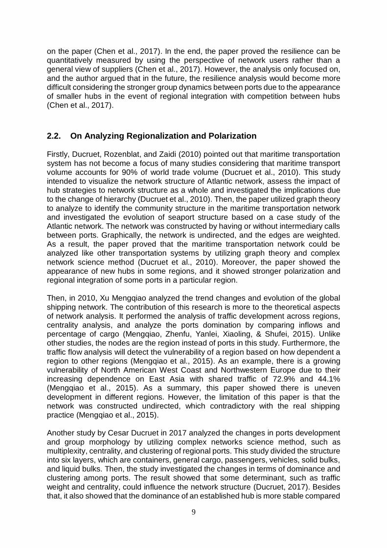
2.2. On Analyzing Regionalization and Polarization Firstly, Ducruet, Rozenblat, and Zaidi (2010) pointed out that maritime transportation system has not become a focus of many studies considering that maritime transport volume accounts for 90% of world trade volume (Ducruet et al., 2010). This study intended to visualize the network structure of Atlantic network, assess the impact of hub strategies to network structure as a whole and investigated the implications due to the change of hierarchy (Ducruet et al., 2010). Then, the paper utilized graph theory to analyze to identify the community structure in the maritime transportation network and investigated the evolution of seaport structure based on a case study of the Atlantic network. The network was constructed by having or without intermediary calls between ports. Graphically, the network is undirected, and the edges are weighted. As a result, the paper proved that the maritime transportation network could be analyzed like other transportation systems by utilizing graph theory and complex network science method (Ducruet et al., 2010). Moreover, the paper showed the appearance of new hubs in some regions, and it showed stronger polarization and regional integration of some ports in a particular region. Then, in 2010, Xu Mengqiao analyzed the trend changes and evolution of the global shipping network. The contribution of this research is more to the theoretical aspects of network analysis. It performed the analysis of traffic development across regions, centrality analysis, and analyze the ports domination by comparing inflows and percentage of cargo (Mengqiao, Zhenfu, Yanlei, Xiaoling, & Shufei, 2015). Unlike other studies, the nodes are the region instead of ports in this study. Furthermore, the traffic flow analysis will detect the vulnerability of a region based on how dependent a region to other regions (Mengqiao et al., 2015). As an example, there is a growing vulnerability of North American West Coast and Northwestern Europe due to their increasing dependence on East Asia with shared traffic of 72.9% and 44.1% (Mengqiao et al., 2015). As a summary, this paper showed there is uneven development in different regions. However, the limitation of this paper is that the network was constructed undirected, which contradictory with the real shipping practice (Mengqiao et al., 2015). Another study by Cesar Ducruet in 2017 analyzed the changes in ports development and group morphology by utilizing complex networks science method, such as multiplexity, centrality, and clustering of regional ports. This study divided the structure into six layers, which are containers, general cargo, passengers, vehicles, solid bulks, and liquid bulks. Then, the study investigated the changes in terms of dominance and clustering among ports. The result showed that some determinant, such as traffic weight and centrality, could influence the network structure (Ducruet, 2017). Besides that, it also showed that the dominance of an established hub is more stable compared

10

to the links (trade flow) that connect the ports (Ducruet, 2017). It is because a strong regional hub usually has their preferential partners and retain the partnership in a long time (Ducruet, 2017). Hence, they can keep the dominance while the links between ports could easily overlap or change over time. As an example, in 1978, liquid bulks represented most of trade flows (visualized by links) from Rotterdam to Ras Tanura or vice versa. While in 2008, the connections from other ports to Rotterdam were dominated by container shipment.

2.3. Research Gaps Based on the literature studies that were presented in the previous section, several research gaps can be identified. Firstly, as discussed previously, complex network science methods were often employed to study vulnerability by performing a targeted attack based on multiple centrality measures as done by Liu in 2017. Calatayud performed another vulnerability study in 2017. The study simulated 80 networks with the focus in the American region. Then, seven nodes were attacked based on multiple centrality measures to see the changes in network performance (Calatayud, Mangan, & Palacin, 2017). The gap from those studies is those studies constructed the network into a single aggregated undirected network while the maritime network has origin and destination which is directed. Since there is always origin and destination in a transportation network, the network should be done in a directed network. It will affect both centrality measures and the topology measurement, which distort the result of the analysis. Furthermore, those networks should not be analyzed by using a single aggregated structure due to multiple layers were embedded into the structure. The reason is that a single aggregation of the network will not consider the rank of the node in each layer, which makes the criticality measurement inaccurate. Hence, the multilayer approach should be employed by doing differentiation in each layer and put the weight in each centrality measurement (De Domenico, Solé-Ribalta, Omodei, Gómez, & Arenas, 2015). Secondly, there is still a lack of researches in General Europe region and multimodality of the hinterland transportation network. By statistics from 1992 to 2017, the study of global Europe region is only 8.75% compared to total geographical focus. Furthermore, research about intermodal terminal and logistics is only 10.52% of total terminologies (Witte et al., 2019). Hence, this study will fill the gap by research the European hinterland transport network holistically instead of focusing on Northwestern Europe only. Thirdly, most of the researches that investigate robustness will often only consider network topology measurement only without addressing the evolution of community structure between layers (to understand how the coalitions are formed and how it evolves across layers) and measure spectral bipartivity in each community. Spectral bipartivity will be useful to know the efficiency of each community cluster, to understand the dynamics, and to understand how strong the collaboration among ports in each cluster and layer (different modal) (Estrada & Gómez-gardeñes, 2016).

11

2.4. Main Research Question Then, based on the research gaps and literature review, the research question can be determined: “How can the criticality of European multimodal transportation network be analytically

assessed by utilizing a complex network science method?” The primary differentiation that differentiate this study is the extensiveness of the complex science method and metrics that are utilized in this study, such as multiple versatility metrics that are used to assess the overall transportation network, the consideration of collaboration and connectivity between critical hubs, and also the community structure that are integrated in this research. Most of the investigations performed those methods independently. Hence, it would lead to an incomplete picture of the solution. Moreover, this study assesses all European region, not only focused on Northwestern European region. Hence, the intention is to give a complete picture of the overall EHTN condition. Besides that, the versatility assessment will also be constructed by using a directed network structure instead of undirected.

2.5. Sub-research Questions To answer the main research question, five sub-questions were determined:

• How can the versatility of European Hinterland Transportation Network be measured by utilizing network theory?

Once the method has been chosen by answering sub-research question number one. Then, the method will be utilized to assess the criticality of EHTN. To answer this research question, firstly, the network structure of EHTN needs to be fully understood. Hence, the analysis will begin from assessing the structure of EHTN, its topology, and interactions that may happen between elements on the network. After that, several centrality or versatility metrics can be determined by matching it with network characteristics of EHTN.

• How can collaboration and connectivity among European container hubs be evaluated based on its modality and network topology?

This sub-research question will answer the gap that is identified during the literature research. While many kinds of research were utilizing multiple centrality metrics, there are a few kinds of research that assess the pattern of collaboration and connectivity among European container hubs. The earlier criticality or versatility assessment intends to provide focus on the most critical container hubs and map the positioning of the hubs in the European region as a representation of the spread of attractors in the network. Then, this particular sub-research question will give an additional point of view in terms of collaboration and connectivity among container hubs. This study will be useful to understand the partnerships between hubs and assess the sustainability of global hub status. The argumentation is by having a large number of competitors (determined by low cooperation index as will be explained in great detail in the relevant chapter), it will

12

affect the sustainability of the hub itself. Moreover, the connectivity will provide information about how well-integrated the hub to the network. The information from this question may be beneficial to the key authorities to map the positioning of specific hubs to the overall network and take measurable actions to achieve global sustainable hubs status.

• How to map the sustainability landscape of European biggest container hubs based on its network structure?

After understanding the competition and connectivity among European hubs by answering the previous sub-research question, it would be essential to understand factors that drive those competitions and assess the sustainability of the hubs based on its network structure and threat from a potential shift of major carriers. For example, it is logical or relevant to assume whether the competition between container hubs are determined by the distance between hubs or not (the first law of geography). Hence, in this research sub-questions, the community structures will be mapped per transportation layers and analyzed. Furthermore, the community structures will also be visualized and mapped into the European map to see the identification of similar communities among hubs in a clear manner. As an example, the high competition (low cooperation index) between Antwerp and Rotterdam is because both of them have the same community, geographically near one another, or other factors drive that relationship. Then, this particular question will investigate the evolution of community structure between layers and analyze whether the hubs tend to stay in the same community between layers or the hubs change layer and do not stay in the same community in other layers.

• How will a network’s performance be affected by removing some particular central or versatile nodes (hubs)?

The impact of the removal of a critical hub will depend on the redundancy of the network itself and the connectivity of a particular hub to the rest of the network. Hence, this sub-question serves as a criticality analysis by measuring three kinds of metrics as a representation of network’s performance from three-point of views, such as degree of integration (also efficiency), coverage, and density (route choices). Targeted disruptions will be performed in each community leader, then the impact to the network’s performance will be measured. Hence, the removal of a critical hub will have a less significant impact compared to less redundant community or network. Then, in this way, the efficiency of the network and the impact of a hub removal can be understood.

• How to provide an informed recommendation based on set information on versatility, community structure, and cooperation-connectivity index?

This final sub-question intends to make an informed decision by combining all analyses that have been performed. Multi-criteria decision-making method will be employed in this section, and an evolution framework is going to be suggested to understand the result and as a guide for the reader.

13

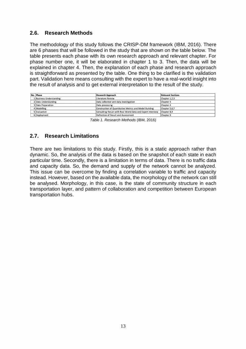
2.6. Research Methods The methodology of this study follows the CRISP-DM framework (IBM, 2016). There are 6 phases that will be followed in the study that are shown on the table below. The table presents each phase with its own research approach and relevant chapter. For phase number one, it will be elaborated in chapter 1 to 3. Then, the data will be explained in chapter 4. Then, the explanation of each phase and research approach is straightforward as presented by the table. One thing to be clarified is the validation part. Validation here means consulting with the expert to have a real-world insight into the result of analysis and to get external interpretation to the result of the study.

Table 1. Research Methods (IBM, 2016)

2.7. Research Limitations

There are two limitations to this study. Firstly, this is a static approach rather than dynamic. So, the analysis of the data is based on the snapshot of each state in each particular time. Secondly, there is a limitation in terms of data. There is no traffic data and capacity data. So, the demand and supply of the network cannot be analyzed. This issue can be overcome by finding a correlation variable to traffic and capacity instead. However, based on the available data, the morphology of the network can still be analysed. Morphology, in this case, is the state of community structure in each transportation layer, and pattern of collaboration and competition between European transportation hubs.

14

2.8. Research Flow The structure of the chapter has been identified in section three of this proposal. As explained before, the study will be divided into three main parts and its chapters to answer the main research questions. The research flow of the study will follow the CRISP-DM framework as shown in figure 4 with additional detail that was not stated in the previous section. Then, each research phase will be grouped into three main sections such as literature review, modelling, and data analytics that are followed by evaluation (multi-criteria decision making and expert interview). As shown by figure 4, the goal and general deliverables are stated in the blue square. Firstly, various concepts will be explored and categorized such as the concepts of versatility, cooperation, and connectivity among ports assessment by following Network-based Hub Port Assessment (NHPA) model. NHPA model is a modelling process to do quantification of port connectivity and port cooperation index based on its network topology and interaction among ports (Low et al., 2009). This modelling process intends to measure the collaboration and competition between ports based on network structure. Moreover, concepts of community detection and spectral bipartivity will be utilized in this study to learn the community structure between ports and how it evolves interlayer. After identifying and categorized those relevant concepts, network topology will be generated based on a service schedule that was issued by Ecorys. The data will be processed in Python and inputted to Muxviz to generate its multilayer structure. Then, various versatility metrics will be quantified by using the concept that was identified before. Based on the centrality measure, ten to twenty most versatile ports will be identified to be analyzed for its cooperation and connectivity by using the NHPA model. The input of the NHPA model is a service schedule that has been modified by focusing on ten to twenty most central port in the network. The output will be the network-based connectivity index and cooperation index. However, this study will be incomplete because we do not know the community structure yet and how it evolves between layers. So, community structure will be investigated by utilizing Multilayer Infomap algorithm that was embedded in Muxviz, and spectral bipartivity will be performed by utilizing the networkx library in Python. Because the community structures will be investigated in each layer, this is part of the hierarchical subgraph method (communities inside communities). Multilayer infomap is an algorithm to detect community cluster in a multilayer network based on network flow and random walk (Martin Rosvall & Bergstrom, 2008). A Sankey diagram can visualize the evolution of community structure between layers. Then, spectral bipartivity is to measure the efficiency of ports topology (Estrada & Gómez-gardeñes, 2016). The lower the bipartivity index can represent a stronger coalition between ports in the same community (Estrada & Gómez-gardeñes, 2016). Furthermore, it also shows a higher efficiency among ports in the same community (Estrada & Gómez-gardeñes, 2016). Lastly, after performing all of the analysis, evaluation of different parts in this study will be integrated and analyzed, which lead to conclusion and recommendation.

15

Figure 4. Research Flow Diagram

16

2.9. The goal of this study The goal of this study is to promote the integration of European multimodal transportation network (EHTN), minimize the inequality in the network, and assess the criticality in the network. This study will do a multifaceted analysis to understand the transportation network structure from a different point of view. This study will assess the criticality of the network and analyzing the community structure to understand the morphology among European hubs. There are several contributions from this study, such as mapping the distribution of the most critical or central hubs in EHTN, understanding the collaboration and competition between hubs, and providing the effect of polarization in EHTN by analyzing the multimodal community structure of ports in European Hinterland. Then, in the end, the landscape of European hinterland transportation network can be understood, and several strategies to promote the integration of European multimodal transportation network can be concluded as a result. Finally, this project is a collaboration between Delft University of Technology and Erasmus University (Rotterdam School of Management).

17

2.10. Research Deliverables Table 2 below summarizes the research questions, methods, and deliverables.

Table 2. Research Questions, Methods, and Deliverables Summary

18

Chapter 3: Concepts

3.1. Integration of Different Types of Modes in Container Transportations

Freight transportation is a very vital component that supports the sustainability of the international supply chain and trade flows (Crainic, 2003). The needs of freight transportations came from the result of demand from consumers that are geographically separated from the producers of the goods (Steadieseifi et al., 2014). It is also a result due to the road transportation cannot be fully depended on due to the extensive movement of goods are required to be efficient at most of the time (Steadieseifi et al., 2014). Hence, more transportation modes were created over time to support the needs of goods delivery. In 2016, for the European region, about 76.4% of inland freights were transported by roads, by rail was about 17.4%, and 6.2% is by waterways (EUROSTAT, 2018). Then, the decision of choosing a particular mode of transportation is by categorizing the goods delivery as per segments, such as pre-haul, long-haul, and end-haul. Pre-haul happens at the beginning of the process, when the goods are picked up (Steadieseifi et al., 2014). Long-haul is a type of transportation that involves a long-distance, such as between cities (Crainic, 2003). Finally, end-haul happens at the end of the process when the goods are delivered to the consumers’ doors (Steadieseifi et al., 2014). The long-haul process usually involves multiple transportation modes (Steadieseifi et al., 2014). However, both of pre-haul and end-haul employs different transportation modes in recent development (Steadieseifi et al., 2014). In the next sections, three types of transportation modes with its characteristics and intention will be fully explained as a bridge to the following sections. Multimodal transportation is the first type of transportations that will be defined in this chapter. Multimodal transportation is a transportation method that requires the involvement of two or more transportation modes (Idri, Oukarfi, Boulmakoul, Zeitouni, & Masri, 2017). The increasing needs of multimodal transportation in the supply chain was mainly driven by the growth of economic development globally (Steadieseifi et al., 2014). Since there is a significant development in the traded goods, a dependence on one mode of transportation only is not enough. One of the factors that gave rise to the use of multimodal transportation is congestion. As an example, the traffic congestion in The Netherlands was tripled between 1985 and 1997 (Dinwoodie & Schijndel, 2000). At that time, the road was dominated by passenger cars and delivery of domestic goods (Dinwoodie & Schijndel, 2000). Hence, the integration between transportation modes was needed. Then, the Transport Structure Plan was ratified in 1990 to reduce car usage (Dinwoodie & Schijndel, 2000). Moreover, the Meerjarenprogramma Infrastructuur en Transport (MIT) was deployed to stimulate investment that encourages the development of major hubs in The Netherlands, such as Rotterdam and Schiphol, improved the development of waterways, and promoted the integration of Rotterdam to the European railway network (Dinwoodie & Schijndel, 2000).

19

However, several factors define the competitiveness and attractiveness of this particular transportation choice by the business community, such as integration of infrastructure, a collaboration between organizations, and also cost competitiveness (Dinwoodie & Schijndel, 2000; Riessen, 2018). In this case, the cost is a crucial component to keep the competitiveness of multimodal transportation to road transportation due to the flexibility of road transportation. Multimodal transportation is less flexible due to the service is offered in a specific time window and the possibility of longer delivery time due to the extension of time is needed when it requires to change the mode of transportation in the transhipment hub or corridors (add reference). To put it concisely, six performance targets could be used as a measurement, such as cost, frequency, delivery time, delivery reliability, flexibility, and safety (Riessen, 2018).

3.2. Hinterland Transportation Modes and Structure As explained in the previous chapters, globalization leads to the rising of regional hubs (Ducruet et al., 2010). Those regional hubs became a central hub in their respective region. Then, in terms of structure, those regional hubs will be supported by and connected to satellite ports. This kind of structure is called a hub-and-spoke network. This particular structure was intended to achieve economy of scale so the logistics cost could be lowered. This can be achieved through a consolidation of the process and employment of multiple transportation modes (Mokhtar, Redi, Krishnamoorthy, & Ernst, 2019). The integration of multiple transportation modes will make the process more efficient, which leads to lower operational costs (Mokhtar et al., 2019). A hub is usually an intermodal terminal which offers multiple-choice of transportation modes (Farahani, Noble, Klein, & Enayati, 2018). In this case, it could be synchromodal or multimodal. The difference is shown in figure 5. As can be seen from the picture, in a synchromodal system, an intermodal terminal connects origin and destination while makes it possible to choose any transportation modes flexibly from one point to another point. On the other hand, a multimodal system does not offer that flexibility. It makes it possible to combine several types of transportation modes. However, there is only one fixed transportation type that connects a particular node and another node. This study will limit the scope to multimodality of European Hinterland Transportation Network. Synchromodal and other transportation system are beyond the scope of this report.

Figure 5. Modes of Transportation (Farahani et al., 2018)

20

3.3. Multilayer Structure in Multimodal Freight Transportation As can be understood from the previous explanation, multimodal transportation consists of different modes. However, there is a fixed link that connects an origin and a destination for a specific mode route. By visualizing it into a single aggregated network, the network is hard to comprehend and is hard to be understood. Furthermore, there is a difference in terms of quantification of centrality rank by using traditional network theory, as explained before. The detail of the differences will be explained in the following section. To have consistency in this report, the term “versatility” will be used when describing a centrality in the multilayer aspect. In multilayer context, the study of multimodal hinterland transportation system can be analyzed by separating the network into different nodes, such as inland shipping, rail, and sea network. Then, the representation of a hub will be determined as a node, while the connection between a particular origin and a destination will be represented as a link or an edge. A more detailed explanation of basic graph theory and its components is included in the appendix section of this report. Moreover, figure 6 provides an example of a multilayer representation of a transportation system in Madrid (Aleta, Meloni, & Moreno, 2017). Multilayer aspects allow consideration of multiple layers within the network, not just focusing on one layer as it is commonly done in single-layer network analysis. Hence, it will enable the examination of interlayer interactions as well as intralayer interaction. In that sense, the importance of a multimodal hub between a variety of layers can be considered (Finn, Silk, Porter, & Pinter-wollman, 2019). Then, it provides a complete picture and insights from the analysis compared to single-layer network analysis.

21

Figure 6. Multimodal Transportation in a Networked System - Transportation Layers in Madrid (Buses, Metro, and

Tram) (Aleta et al., 2017)

The goal of this section is to explain the representation of multimodal freight transportation system in the networked system. Hence, by doing a representation in the networked system, then the structure of multimodal freight transportation can be studied and analyzed further by utilizing network theory. The following section will introduce the definition of a multilayer network and its application in transportation research. Then, it will be followed by an explanation of multiple types of multilayer network and provide argumentation why multimodal freight transportation system can be studied in multilayer context.

22

3.3.1. Definition of Multilayer Network The population in 30 world’s megacities in the world has roughly half a billion people currently (Gallotti, Porter, & Barthelemy, 2015). Based on that background, there is an increasing development of multiple modes of transportation infrastructure. Hence, the transportation networks have a growing complexity on the way of its development as well (Gallotti et al., 2015). In megacities or advanced economies region, the unavailability of infrastructures to access some regions is not a problem. However, to find an optimal route from one place to another place becomes the main interest. Optimal means less travel time, shortest distance, or fewer transportation modes change. Specifically, related to transportation modes, many transportation modes can be chosen from one origin to a destination. However, to find the optimal and efficient routes from one point to another point have developed the curiosity of many researchers, transportation providers, or technological companies (Gallotti et al., 2015; M. Rosvall, Trusina, Minnhagen, & Sneppen, 2005). As an example, when a traveller wants to go from one place to another place in one of the world’s biggest megacities, such as Hong Kong, Tokyo, or other cities which have different and complex transportation networks, it is problematic to make an efficient choice to go the destination if the traveller only relies on his or her mental maps and visual working memory (Gallotti et al., 2015). It is because of the limitation of the human itself to process a large amount of information. By breaking down the full networked system into multiple subsystems and layers, it will provide more precise insight and improve the understanding of the networked system itself. The separation of a complex network into different layers with an interlayer connection between each layer is called multilayer network (De Domenico et al., 2013; Finn et al., 2019; Kivelä et al., 2014). Considering the interactions between different layers in the multilayered network, methodological tools in “traditional” network theory was deemed to be insufficient (De Domenico et al., 2013). According to De Domenico (2013), available methodological tools in “traditional” network theory cannot explain the multiplexity characteristics in the multilayered network due to an insufficient mathematical framework to explain those behaviours (De Domenico et al., 2013). A tensorial approach that was developed by Manlio De Domenico, et al. in 2013 can provide insights, such as influence in multi-channel social media networks and multimodal transportation networks (De Domenico et al., 2013). Multilayer network may tell different information that is different from traditional network theory. For example, the multilayer analysis might detect various leaders or central nodes in a group that are not considered in conventional network theory due to a different approach that is employed (De Domenico, Solé-Ribalta, et al., 2015; Finn et al., 2019). Then, in the context of a transportation system, the multilayer approach refined the analysis of efficiency of transportation networks (Finn et al., 2019). Moreover, in the spreading of information context, multilayer approach can expose the difference in influence in different communities that were left unnoticed in traditional or monolayer network (Finn et al., 2019). The next section explains the types of multilayer network as an introduction before going to multilayer application in multimodal freight transportation.

23

3.3.2. Types of Multilayer Network As stated previously, De Domenico (2013) and Kivela, et al. (2014) proposed a mathematical formulation to formalize the application of multilayer method to a real-world case (De Domenico et al., 2013; Kivelä et al., 2014). The fundamental difference between the multilayer approach and traditional network theory is the differentiation of layers. In a single layer network, all of the interactions will be presented. On the other hand, in multilayer approach, the network will be separated into different layers which each layer presents a distinct type of interactions (De Domenico, Nicosia, Arenas, & Latora, 2015; Finn et al., 2019). For example, in the air transportation system, differentiation of airlines can be presented in different layers (De Domenico, Nicosia, et al., 2015; De Domenico, Solé-Ribalta, et al., 2015). Moreover, in the urban transportation system, the network can also be represented into different transportation modes, such as tram, bus, and metro (Aleta et al., 2017). Then, in multilayer maritime transportation system, the layers can be as a dominant traffic type, such as containers, general cargo, and bulks with the nodes are the hubs and ports while the links are the travel-path from one port to other ports (Ducruet, 2017). Multilayer networks can be specified into two types, such as a multiplex network (edge-coloured network) and interconnected network (node-coloured network). Multiplex is a network which has several layers and shares the same nodes across the layers (Finn et al., 2019; Kivelä et al., 2014). Then, considering the inter-layer connection, only the same nodes between layers can connect as can be seen in figure 7 (Finn et al., 2019). The other name of the multiplex network is edge-coloured network. It is called edge-coloured to label the edges which have the same colour to connect the nodes that are incident to each other across layers (Finn et al., 2019; Kivelä et al., 2014). It is possible to divide the multiplex network into two aspects, which is categorical and ordinal (Kivelä et al., 2014). Ordinal multilayer network is where interlayer edges are present in a layer that are adjacent to each other while categorical multilayer network shows all of the possible combinations of interlayer edges (De Domenico, Porter, & Arenas, 2014; Kivelä et al., 2014). However, as mentioned before, in edges-coloured network or multiplex network, the interlayer edges only connect the same nodes in different layers. Another type of multilayer is an interconnected network or often be called by a node-coloured network. The difference to the multiplex network is the possibility to connect different nodes in different layers (Finn et al., 2019). Interlayer edges do not have to join the same nodes as it is the case for a multiplex network. In a multiplex network, it is very crucial to have similar nodes that allow the interlayer connection. Hence, if there are no same nodes across layers, then it is impossible to have an interlayer connection. While in a node-coloured network, the nodes can represent different entities (Finn et al., 2019). Therefore, the interlayer edges can facilitate a connection of different types of nodes between layers (Kivelä et al., 2014). Moreover, another difference is in the focus of network components. In node-coloured network, the nodes that have the same types are assigned with the same colour (Kivelä et al., 2014). In this context, the nodes in the same layers have the same colour, and each layer can be differentiated by the colour of the nodes. While in an edges-coloured network, the

24

emphasis is in the interlayer connection that connects the same nodes between layers. Then, the edges that connect the same nodes have the same colour.

Figure 7. Edge-Coloured Network (De Domenico, Solé-Ribalta, et al., 2015)

Figure 8. Node-Coloured Network (Kivelä et al., 2014)

25

3.3.3. The Role of a Hub in Multimodal Freight Transportation System A hub is a central facility that acts as an intermediary to do a consolidation of services or freight flows from different origins and destinations (Mokhtar et al., 2019; Ramaekers, Verdonck, Caris, Meers, & Macharis, 2017; Rodrigue, Debrie, Fremont, & Gouvernal, 2010). In the context of multimodal freight transportation, the consolidation of freight movements is useful to achieve efficiency and economies of scale; hence, the logistical costs can be kept low, and good quality of performance can be maintained (Tavasszy & de Jong, 2014). Furthermore, ports can also act as a gateway to a particular region (Fleming & Hayuth, 1994). According to the study by D.K. Fleming and Y. Hayuth (1994), a central container hub or port plays an essential role to spin a national economic wheel and promote regional economic development (Fleming & Hayuth, 1994; Y. Wang & Cullinane, 2016). Central means that a particular hub has an influential role that determines the development in the community (Finn et al., 2019). A central hub needs multiple intermediaries around its proximity to channel the traffic from origins to the hub itself (Fleming & Hayuth, 1994). In this case, the intermediary hubs can be intermediate or central as well (Fleming & Hayuth, 1994). Because of this reason, the establishment of a central hub will trigger the development of transportation infrastructures to support the role of hubs and intermediary ports. Hence, it will induce the development of trade, and the benefited area will have more economic activities (Fleming & Hayuth, 1994). As in the case in the development of Yangtze River Delta (YRD) in 1970, as a central corridor and gateway in China, has changed Shanghai into a famous global city and hub. It has also driven Shanghai’s specialization in many sectors to support the economic activities of the ports itself, such as the assignments of large urban areas to increase the performance of cargo transfers and industrial activities in the port’s proximity (C. Wang & Ducruet, 2012). Moreover, Wang and Cullinane (2016) stated that the location of a more central port could attract more goods movement from the hinterland, like the case of Le Havre in Northern European region (Y. Wang & Cullinane, 2016). Furthermore, there are two types of hubs, which is relay ports and load centre ports (Fleming & Hayuth, 1994). Relay ports are located in the middle of major sea routes, and it is a very crucial point that connects multiple container flows (Fleming & Hayuth, 1994). Hence, structurally, there is a visible pattern from and to neighbouring areas that are surrounding this nodal point (Fleming & Hayuth, 1994). On the other hand, those hubs only generate little traffic like the case of Singapore (Fleming & Hayuth, 1994). Another type of hubs is called load centre hubs. The distinction with relay ports that those hubs also generate a large proportion of traffic from its surrounding hinterland (Fleming & Hayuth, 1994).

26

3.3.4. Measuring Centrality of Multilayer Network To have consistency throughout the report, the term versatility will be used when discussing centrality in multilayer context. However, before going to the detail explanation of centrality and versatility, the introduction of basic centrality concepts will be explained in this section. In multimodal transportation context, centrality measurement will be useful to measure the relative importance of a hub to other hubs within the region (Finn et al., 2019; Y. Wang & Cullinane, 2016). Hence, it is logical to suspect the hubs that have significant centrality value to other hubs as influential and play a crucial role in the defining the behaviour of the network (Finn et al., 2019). There are several designed concepts in centrality analysis. For example, degree centrality is the most straightforward measure in this context (Y. Wang & Cullinane, 2016). Degree centrality measures the number of connections from and to a particular node to evaluate its relative importance in the network (Fletcher & Wennekers, 2018). In the context of multimodal freight transportation, a degree is a number of a direct connection from/to a particular hub (as an origin or a destination; defined as a node). The flaw of this approach is that this approach does not consider an indirect link to a node (Y. Wang & Cullinane, 2016). Moreover, another approach is based on the preferential-based attachment. In this context, a node or a hub that has a high degree will also be attached to a node that has a high degree. It can be understood as a more influential node will prefer a connection to a well-connected node as well (Y. Wang & Cullinane, 2016). This approach is called the eigenvector centrality. It has been implemented by Wang and Cullinane (2008). However, this approach only considers a single layer network instead of analyzing it in multilayer context. Wang and Cullinane (2008) developed a network based on liner shipping network where the nodes are the ports, and the link is based on liner shipping services (Y. Wang & Cullinane, 2008). The Wang and Cullinane (2008) showed that the ports that have a high eigenvector centrality have a high competitiveness relative to other ports (Y. Wang & Cullinane, 2008). However, the flaws in the analysis are that the study was done in single layer context and undirected network. Another centrality measure is PageRank centrality. PageRank centrality has a close relation to eigenvector centrality. PageRank is an algorithm that is utilized by a prevalent search engine, which is Google (De Domenico, Solé-Ribalta, et al., 2015). This centrality measure has been utilized by Fletcher and Wennekers (2017) to study neuronal activity (Fletcher & Wennekers, 2018). The detail and operationalization of PageRank centrality will be explained in the following section.

27

3.4. Ranking the Importance of a Node in Multilayer Network

A hub can have a few numbers of degree connections in each layer or a particular network of a specific transportation mode, but that particular hub is present in all layers. Hence, it can provide a more significant impact on the network across layers (De Domenico, Solé-Ribalta, et al., 2015; Finn et al., 2019). That central hub can be considered as a versatile hub (or node) in a multilayer context (De Domenico, Solé-Ribalta, et al., 2015). Throughout this study, a term versatility or versatile will be used when discussing centrality in the multilayer context. Otherwise, a term centrality will be used when discussing a central node in a single layer network context. Figure 9 presents an illustrative case about versatility in multilayer context and explains the difference in terms of ranking the importance of a node between the multilayer network and single-layer network. The illustrative example was presented by De Domenico, Solé-Ribalta, et al. (2015) in a paper about versatile nodes identification in multilayer networks. As explained in the paper by De Domenico, Solé-Ribalta, et al. (2015), this is a case to measure author’s contribution to a research article, and it can be evaluated by measuring versatility in the network (De Domenico, Solé-Ribalta, et al., 2015). According to figure 9, there are five authors in the illustrative case, such as AA, BB, CC, DD, and EE. The nodes are the authors. Then, the corresponding research activities were separated into different layers in the context of the multilayer network. A link can be formed when there are two or more authors were engaged in similar research activity. This is an undirected network and unweighted network where all links have the same weight, or the weight was assigned uniformly for all connections. The resulting aggregated network can be seen in figure 9(b). The resulting ranks from the aggregated network and multilayer network were showed by figure 9(c). To understand the methodology easily, the concept of layering and degree of connections become the main point of interest. In a single layer aggregated network, all of the present connection of all nodes will be combined into a single layer network. Hence, as figure 9(b) showed, all of different contributions and links of interactions will be aggregated into the same layer, and all nodes with its connections will be exhibited and evaluated in the same network layer. Hence, it may be possible where all nodes have the same degree of connections, and therefore, have the same rank. Figure 9(b) shows that each node has four degrees of connections. The methodology is different in the multilayer network. The research contributions, as in the illustrative case, were separated into different layers. After that, the rank from each contribution will be evaluated and ranked separately per layer. Then, the aggregated rank has resulted from the consensus of all rank from those separate layers. Therefore, in this illustrative case, the multilayer approach provided different result compared to a single aggregated network approach. While the single aggregated network presented the same rank for all authors, the multilayer network presented different rank of the authors with author CC has the highest rank compared to all authors. In summary, in this context, the multilayer approach provided with a more holistic approach in measuring the importance of authors’ research contributions. The role of CC is often underestimated by using a more traditional approach. However, in the multilayer approach, CC can be seen connecting two layers of the most significant contributions, which is “conceived and designed the

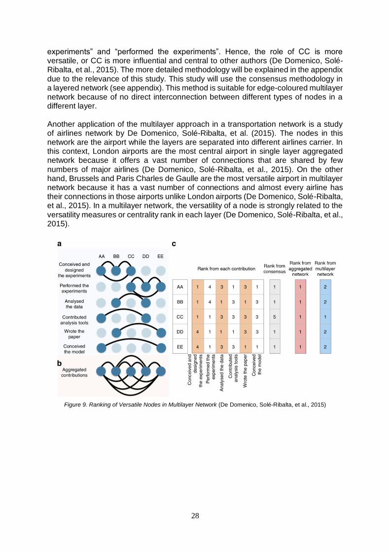
28

experiments” and “performed the experiments”. Hence, the role of CC is more versatile, or CC is more influential and central to other authors (De Domenico, Solé-Ribalta, et al., 2015). The more detailed methodology will be explained in the appendix due to the relevance of this study. This study will use the consensus methodology in a layered network (see appendix). This method is suitable for edge-coloured multilayer network because of no direct interconnection between different types of nodes in a different layer. Another application of the multilayer approach in a transportation network is a study of airlines network by De Domenico, Solé-Ribalta, et al. (2015). The nodes in this network are the airport while the layers are separated into different airlines carrier. In this context, London airports are the most central airport in single layer aggregated network because it offers a vast number of connections that are shared by few numbers of major airlines (De Domenico, Solé-Ribalta, et al., 2015). On the other hand, Brussels and Paris Charles de Gaulle are the most versatile airport in multilayer network because it has a vast number of connections and almost every airline has their connections in those airports unlike London airports (De Domenico, Solé-Ribalta, et al., 2015). In a multilayer network, the versatility of a node is strongly related to the versatility measures or centrality rank in each layer (De Domenico, Solé-Ribalta, et al., 2015).

Figure 9. Ranking of Versatile Nodes in Multilayer Network (De Domenico, Solé-Ribalta, et al., 2015)

29

3.5. Operationalizing Versatility Measurement in Multimodal Freight Transportation

Several metrics need to be defined to measure the versatility of a node in the multilayer network. In this section, the relevance of a particular metrics to the case study of European multimodal transportation network will be explained. Therefore, the intention of why such metrics are used can be understood.

3.5.1. Degree Versatility Degree centrality is a traditional approach to measure a degree of centrality or versatility of a node in a network (Y. Wang & Cullinane, 2016). This centrality measure was initially proposed by Freeman (1979). The traditional representation of degree centrality is mathematically formulated as (Freeman, 1979; Y. Wang & Cullinane, 2016):

𝑲𝒊 = 𝑪𝑫(𝒊) = ∑ 𝑿𝒊𝒋

𝑵

𝒋

The mathematical equation above means that the degree centrality or versatility of a particular node i can be measured by several direct connections to/from that specific node (Fletcher & Wennekers, 2018). In this case, i is a focal node, j is the nodes that have a direct connection with the focal node, N is a number of the nodes in the network, and 𝑿𝒊𝒋 is an established connection between node i and node j. The resulting

interaction can be either 1 or 0, depending on the existence of the connection between the focal node and node j. However, throughout the time, another degree centrality variance was defined by considering the weight of the connections or links. As mentioned by Fletcher and Wennekers (2018), the mathematical formulation of weighted degree centrality is defined as:

𝑺𝒊 = 𝑪𝑫𝑾(𝒊) = ∑ 𝑾𝒊𝒋

𝑵

𝒋

The difference with the previous equation is in terms of assigning a weight to an established connection (Fletcher & Wennekers, 2018). If in the previous definition, an established connection will result in 1 as a value. In the weighted equation, the value of the interaction depends on the strength of the connection (Fletcher & Wennekers, 2018). However, the disadvantage of this centrality measure is it does not consider the degree of influence of a node, in other words, are indirect connections, when doing attachment to a particular node (Y. Wang & Cullinane, 2016). The previous degree centrality measures were defined for a single layer network. However, the logic of how it works will be similar in multilayer context; the distinction is only in terms of interlayer connection. The mathematical formulation of degree versatility in multilayer network is:

30

𝑲𝜶 = ∑ 𝒌𝜶(�̃��̃�)

𝑳

𝒉,𝒌=𝟏

𝒌∝(�̃��̃�) is a degree versatility that is related to a connection between layer h and k (De Domenico et al., 2013). The relevance in the context of multimodal freight transportation network is this is a very logical and most straightforward method to measure the importance of a node by aggregating the number of direct connections to a focal hub. The more total connections that a hub has across the layers of different modes. Therefore, the more critical the hub is. The limitation is the same as the fundamental limitation as stated in the mathematical formulation that this quantification of importance does not consider the “weight” or “influence” of other hubs that have a connection to the focal hub.

3.5.2. Eigenvector Versatility Eigenvector versatility overcomes the limitation in degree versatility measures. The eigenvector method will consider the influence of other nodes that are attached to the focal node (Fletcher & Wennekers, 2018; Y. Wang & Cullinane, 2016). Hence, a node is more influential or considered holding a central role if there are more influential nodes that are connected to the focal node (Fletcher & Wennekers, 2018; Y. Wang & Cullinane, 2016). The calculation of eigenvector versatility is started by assigning 1 to all versatility (for multilayer) or centrality measures (for a single layer). Then, the centrality or versatility values can be evaluated by solving the below equation:

𝑪𝑬(𝒙) =𝟏

𝝀∑ 𝑪𝑬

𝒚→𝒙

(𝒚)

After solving the mathematical formulation, it can also be written as:

𝝀𝒆 = 𝑨𝒆 Solving e in the above equation will result in the eigenvector versatility or centrality for all nodes. λ is the largest eigenvalue for adjacency matrix A (Fletcher & Wennekers, 2018). Generalization of Eigenvector centrality in multilayer context is formulated as below:

𝑽𝜷𝜹 = 𝝀𝟏−𝟏𝑴

𝜷𝜹

𝜶�̃�𝑽𝜶�̃�

The step by step process of solving the equation is similar to the method in monoplex (single-layer network) by solving for 𝑽𝜶�̃� iteratively (De Domenico et al., 2013).

As stated in section “Measuring Centrality in Multilayer Network”, eigenvector centrality measure has been implemented by Wang and Cullinane (2008) in a single layer network. In multimodal freight transportation, this measure will be beneficial to rank the influence of major European hinterland hubs. A hub can be more critical or

31

influential if the hub connects to more central hubs. Hence, its role is very vital in the multimodal network.

3.5.3. PageRank Versatility PageRank centrality has a correlation with eigenvector centrality (Fletcher & Wennekers, 2018). This algorithm is based on steady-state formulation of a random walker within the network by trying to visit every webpage on the internet (Brin & Page, 1998; De Domenico, Solé-Ribalta, et al., 2015; Fletcher & Wennekers, 2018; Kivelä et al., 2014; Page, Brin, Motwani, & Winograd, 1998). In this context, a random walker moves from one node to the neighbouring node with rate r and also does teleportation with rate r’ (Brin & Page, 1998; De Domenico, Solé-Ribalta, et al., 2015; Page et al., 1998). Mathematically, as proposed by De Domenico, Solé-Ribalta et al. (2015), the equation of PageRank in an interconnected multiplex network is:

𝑹𝒋𝜷𝒊𝜶 = 𝒓𝑻𝒋𝜷

𝒊𝜶 +(𝟏 − 𝒓)

𝑵𝑳𝒖𝒋𝜷

𝒊𝜶

The above definition is valid for all multiplex networks which have either ingoing or outgoing edges or both of edges types (De Domenico, Solé-Ribalta, et al., 2015). As explained briefly in the first paragraph, this algorithm is based on a random walker that moves within the network. It is often called the “random surfer model” (Fletcher & Wennekers, 2018). To simplify the explanation, this report explains in terms of a random walker in single layer network. It works similarly in a multilayer network except with the extension of a definition based on a tensorial approach and additional component in the equation to define the probability of the random walker does teleportation from one layer to another layer. This study will not include the technical details of the PageRank algorithm in the multilayer network due to the different context of this study. This study will limit to the application of PageRank versatility measures in multimodal freight transportation. The way of this algorithm works can be easily understood by imagining the movement of a webpage visitor as described by Fletcher and Wennekers (2018) in their study about measuring the centrality of neuron networks. It is necessary to define a visitor starting point in the network. Assume the visitor stands on a particular node (webpage). When the user opens another webpage or clicks another link, the user made an outgoing direction to a new node. There is also a possibility as defined in the equation that the user makes teleportation from one node to another node that is indirectly connected one another as if the user jumps to another part of the network. This process will be done recursively. Finally, the webpages will be ranked as per its number of visitors (De Domenico, Solé-Ribalta, et al., 2015; Fletcher & Wennekers, 2018). That is its PageRank centrality measure.

3.5.4. Katz Versatility In the case of a directed network like multimodal network, eigenvector measure can lead to a wrong result because eigenvector approach will result in 0 for a node that

32

has only outgoing edges (De Domenico, Solé-Ribalta, et al., 2015). This flaw in the analysis can be overcome by Katz centrality method (for a single layer) or Katz versatility (for multilayer network) (De Domenico, Solé-Ribalta, et al., 2015). Moreover, Katz centrality is a derivation of degree centrality measure. Degree centrality has a flaw that it does not take into account the influence of the nodes that are located far from the focal node, in other words, an indirect connection of nodes in the proximity (Fletcher & Wennekers, 2018; Y. Wang & Cullinane, 2016). As stated in the paper by Fletcher and Wennekers (2018), the mathematical formulation of Katz centrality is a monoplex network is:

𝑪𝑲(𝒙) = ∑ ∑ 𝜶𝒌

𝒚→𝒙𝒌

∞

𝒌=𝟏

𝜶 represents the cost factor of a node. It means the node will have fewer contributions the farther it is located by x (Fletcher & Wennekers, 2018). k defines a number of hops

from a particular node. Then, the range of 𝜶 is defined as 𝟎 < 𝜶 <𝟏

𝝀𝒎𝒂𝒙 (Fletcher &

Wennekers, 2018). 𝝀𝒎𝒂𝒙 is the largest eigenvalue which defined the value of the cost factor (Fletcher & Wennekers, 2018). In the case of the multilayer network, it will follow the same algorithm and calculate the centrality value layer by layer. Then, finally, do a consensus to evaluate the rank of the versatility of a node in the multilayer network (De Domenico et al., 2013; Kivelä et al., 2014).

3.6. Multimodality and Multiplexity Multiplexity measurement is a representation of the multimodality of a transportation network. This measurement will be used in chapter 5. Multiplexity is a ratio that compares the availability of a transportation mode in a particular location and the availability of all transportation mode in existence. For example, Rotterdam has three transportation system in existence, which consists of the sea network, the inland network, and the rail network. Hence, the multiplexity of Rotterdam is 1, which is resulted from the ratio of three transportation network that is available in Rotterdam and three transportation in existence. Should a location only have one transportation network compared to three transportation networks in total (the total or a maximum number of transportation network types that are available in the network); then, the multiplexity number will be 0.33 (1/3).

33

3.7. Inequality in The European Multimodal Transportation Network Once the versatility of the network has been identified and operationalized. The next analysis will be to analyze and investigate the community structures that are formed around the most versatile locations in the network. The community identification in the multilayer network will utilize the multilayer infomap algorithm (Domenico, Lancichinetti, Arenas, & Rosvall, 2015). This algorithm is an extension of original infomap algorithm for community detection in a single aggregated network (Bohlin, Edler, Lancichine, & Rosvall, n.d.; M Rosvall, Axelsson, & Bergstrom, 2010; Martin Rosvall & Bergstrom, 2008). The base algorithm is called the map equation (M Rosvall et al., 2010). Once the community identification has been done and the group of clusters around the most versatile locations can be detected, then the objective of this section is to explore the inequality in the network, as it is called “The Matthew Effect”. This term was originated from Robert K. Merton in 1968. The intention of investigation of this effect in this study is to show the accumulation of benefits which happens in the network which contributes to the polarization and the criticality or sensitivity in the network to targeted disruptions.

3.8. Community Formation, Cooperation between Hubs, and The First Law of Geography

Furthermore, related to the community formation in the network, it is also determined by “the first law of geography” which was originated from Waldo Tobler in 1970. The study of Waldo Tobler mentioned that the correlation is higher in the things that are more closely related to each other rather than distant things (Tobler, 1970). Based on community detection, it is possible to have several hubs that are located in the same community structure. Hence, it could be supposed that those hubs have a more competitive relationship due to the overlaps of the regions that are served by those hubs in the community.

34

3.9. Chapter Summary and Conclusion This chapter presents the literature review and the fundamental theories of this study. There are several parts in this chapter that are consisting of the theory from multilayer analysis, versatility analysis, community detection, and the relationship between cooperation and the first law of geography. As stated earlier, the intention of this chapter is also to explain the relationship between three main building blocks to support the final analysis (criticality analysis) in this study. This chapter provided an operationalization and the fundamental information as well as the purpose of the investigations that were performed in this study. As a summary, the versatility analysis determined the most versatile container hubs in the network. Hence, it will set the focus of the study. Then, the following analysis, which is the community structure analysis provides information about the clustering formation around the most versatile hubs. The clustering analysis will set as the primary foundation for the criticality analysis and also served as a boundary for inequality or inspection of the Matthew effect in the network. The last part of the main building blocks is the cooperation and connectivity analysis, which intends to investigate the application of the first law of geography in the European multimodal transportation network. It will also provide information about the sustainability of the hubs, as will be explained in detail in chapter 7 and 9.

35

Chapter 4: Modelling Framework

4.1. Framework for Measuring Versatility of EHTN There is three primary part analysis to study versatility, the correlation and connectivity between European hubs, and community structure of European transportation hubs. Throughout this report, the CRISP-DM method will be employed to process, analyze, and evaluate the result of the data, as shown in figure 10. CRISP-DM is a structured framework to execute a data analytics project (IBM, 2016).

Figure 10. CRISP-DM Framework (IBM, 2016)

The CRISP-DM framework consists of six steps process, such as (IBM, 2016): 1. Business understanding 2. Data understanding 3. Data preparation 4. Modelling 5. Evaluation 6. Deployment

The goal of each process is as follow: Business understanding is a process to understand the specific intentions and set of criteria that want to be achieved by the organization we serve or our client (IBM, 2016). The objective of this particular process is to know possible challenges in advance, important goals of the organization, and resources available to work on the project (IBM, 2016). Data understanding is intended to have a deep understanding of the shape of the data, what kind of information is supplied by the data, how it relates to the analytical objective, and it is also essential to understand of the quality of the data itself (IBM, 2016). This step is very relevant to avoid difficulties and minimize the unexpected risk in the long run (IBM, 2016).

36

Data preparation is a stage where the analyst does data processing. It consists of three steps processes, such as data selection, data construction, and data integration (if needed) (Smart Vision Europe, 2018). This step is the most time-consuming steps in a project which consumes 50% to 70% time spent and effort (IBM, 2016). Modelling is a step after the analyst has been done with the data preparation step. In this step, multiple analysis will be carried on by utilizing the relevant modelling techniques (IBM, 2016). This step is often done in several iterations. The data that has been pre-processed will be inputted into the model. Then, the analyst will check the output data and analyze it further whether the data can provide some insight and whether the data can answer the research question in a satisfactory manner (IBM, 2016). The main intention of this step is to get some insights based on modelling techniques of choice. Evaluation is a step where the analyst measures the output from modelling to business or initial objectives of the client and the analysts themselves (IBM, 2016). In other words, the analyst will assess the results from the modeling step and do the interpretation of the result (Smart Vision Europe, 2018). The deployment consists of a plan to do an improvement to the client’s organization or institution based on the analyst’s research result (IBM, 2016). Some steps have been explained in the previous chapter. Hence, this chapter will only do a detail explanation of some relevant steps that result in the interpretation from the result of modelling steps. Business understanding will not be part of this chapter because it has been explained in great detail in chapter one and two of this report. Business understanding will be related to the explanation of the background information and how this study can be useful and to which organization which has been discussed in chapter one. Chapter two of the study is related to research objective and knowledge gaps which is relevant to business understanding step as well. Data understanding and data preparation will be combined into one section which will be titled data processing. In this section, input raw data will be explained and what kind of information are available from the data. However, the data will not be fully disclosed due to the data is proprietary and confidential. There is some amount of sensitive information that is contained in the data. The steps of data processing will be explained here. Then, the data will become an input to the modelling software that is used in this study. Furthermore, the modeling step will explain the specific process that was carried on in this study. Then, some relevant criteria and evaluation indicators will be presented as a result of the modelling step. Finally, evaluation and deployment will be titled as the interpretation of the versatility ranking of multimodal European Hinterland Hubs. In this section, the result of the model will be deeply discussed, analyzed, and investigated. Afterwards, the conclusion will be presented at the end of chapter four.

37

4.2. Data Processing

4.2.1. Initial Data Specification Initial data was provided by Camill Harter from the Erasmus University of Rotterdam. Ecorys supplied this data for research. However, this data is proprietary, which consists of some sensitive and confidential information that cannot be disclosed. Hence, the data will not be fully disclosed, and the data will only fully be elaborated by a written explanation. The data is an annual shipment schedule data (2019 shipment schedule) that entirely covered all European region hinterland transportation schedule. Below is the information that can be extracted from the data: 1. Origin terminal consists of information about the country code, country name, city, and name of the terminal. 2. Destination terminal consists of the same structure of information like the one in the origin terminal. 3. Modality is a type of transportation mode that connects a particular origin and the destination terminal. 4. Carrier is the name of the specific service that is used to deliver the shipment from the origin terminal to the destination terminal. 5. Weekly schedule of shipping frequency. The data also supply the exact frequencies of the shipping schedule on a particular day. 6. A number of departures per week. This field is the aggregation value of the weekly frequency. 7. Transport time (days) is a travel time required for one vessel from the origin terminal to the destination terminal. Another data is a set of European cities and coordinates, which will be combined into one source of information. The information of European cities and its coordinates will later be used for network construction and visualization after versatility measurement.

4.2.2. Data Preparation Both of the data about the shipping schedule and the coordinates of European cities were combined into one table. Hence, the data supplies both information about the shipping schedule and exact coordinates. The objective of the usage of this shipping schedule is to construct the entire European hinterland transportation network. The network will include its multimodal transportation network. In that way, a complete picture can be concluded by analyzing its network structure. The data was processed through structured steps which will be listed shortly, and each step has its objective. The structured steps of data preparation: 1. Data modification to separate some “merged” information, such as separation of merged information in origin terminal and destination terminal. Origin terminal and

38

destination terminal consist of four different information. Hence, this step intends to separate those “merged” information into independent fields. In that way, it will reduce complexity to process the data. Moreover, the same treatment will be done into the carrier field to separate carrier code and carrier name. 2. Then, the data will be prepared to be transformed as per Muxviz requirement. Muxviz is a package in R to do multilayer network analysis, specifically versatility analysis. The reason behind the choice of this package with the explanation of how to install and use Muxviz will be done in the appendix section. 3. The output from Muxviz will then be processed in Python with all supporting packages, such as pandas, numpy, and scikit-learn (package for machine learning to do principal component analysis). The objective of this step is to determine the essential versatility indicators and rank the ports by doing a preference-based ranking method. The preference-based ranking method is Borda count, and it is a method to have a single ranking based on a consensus of the most essential versatility metrics.

4.3. Modelling

4.3.1. Network Initialization Network generation, versatility diagnostics, and network analysis were performed in MuxViz, while all data processing and evaluation were carried on Python with basic packages, such as networkx, pandas, numpy, seaborn (for visualization), and scikit-learn for machine learning (when conducting principal component analysis method). There are three main input files for Muxviz: 1. Configuration file. This file defines the path in the computer to do the network analysis. 2. Layout file. This file consists of the list of nodes with its identification number. Moreover, the coordinates information will also be defined in this file if needed. 3. Edges list file. This file is the most crucial file to generate the network. It has information about the point of origin and the destination node that is represented by node identification number. If the link is weighted, it will also be defined by using this file. In this study, there are three edges-list files in total because there are three layers to be analyzed in this research, such as inland shipping, rail, and sea. Once Muxviz generated the network by using the inputted files. Then, the versatility analysis can be run by using Muxviz’s feature. Multiple versatility metrics can be used to diagnose the versatility of the multilayer network. The reasoning of why specific metrics were chosen has been fully explained in chapter three, including the mathematical formulation of the metrics. Once the diagnostics were executed and done, then the output of versatility analysis can be converted into a .csv file. Then, the rest of the evaluation will be done in Python.’

39

4.3.2. Modelling of Versatility Analysis in Python Principal Component Analysis method will be employed in this step. The objective of this method is for dimension reductions. In other words, if there are many descriptors in the data, it will be needed to choose only the most crucial descriptors that will be sufficient to cover all information that is contained in the data. Represent all descriptors will often add complexity and blurred important information. Hence, this method is used for that purpose. Moreover, the descriptors that are used will be ranked by how much they can cover the variance of overall data. Then, the data will be plotted against two most significant component to describe the data and check the distribution of the data in 2D axis (consists of principal component one (PC1 for short) in one axis and principal component two (PC2)). By plotting the data on the axis, the cluster of the data will be visible. Then, the cluster can be analyzed further to see the distance between clusters and how a similar type of data is grouped. Please refer to figure 11 for the snapshot of versatility table as a result of Muxviz. Since this data is already modified and obscured the original information of the original data, the snapshot can be shown in this case. The original data, which is the shipping schedule is proprietary. However, the output table from Muxviz has a different structure with all versatility metrics without containing any information about shipping schedule. There are two kinds of tables which is unweighted and weighted. The former is the versatility result with has no weight assigned on the links ports. On the other hand, the latter is the versatility result with weighted connections between cities.

Figure 11. Versatility Output Table from Muxviz

40

The table that is shown above is the weighted versatility result from Muxviz. However, the unweighted table will look similar to the difference in the result. The degree metrics will have the same result since it is the most traditional approach and degree is not affected by the weight of the link; instead, it will only count a number of incoming and outgoing links on a node. The most noticeable difference is on the strength value between weighted and unweighted versatility result. For unweighted, strength is the same as a degree because there is no weight assigned. However, with weight, the value of the strength will be determined and influenced by the weight of the link (see chapter three for a detailed explanation in the degree section). To have a further analysis of clustering or grouping in PCA, it is necessary to decide how the data can be grouped. In this case, two metrics can be used to group the data. Firstly, it is by multiplexity. Multiplexity provides information about the ratio between a number of layers which a node presents and a total count of the layers. For example, the multiplexity value of Aalborg city is 0.33, which means the city only has one type of transportation. If the value of multiplexity is 1, like the case for Rotterdam, then it has all types of transportation. In other words, Rotterdam presents in all transportation layers. The data can be grouped into three values of multiplexity, which is 0.33, 0.67, and 1. The next step is to decide and rank the principal components by using multiplexity to group the data. The result will be explained in detail in another section. The data is also grouped by K-Core value. The K-Core concept has been explained in chapter three. For principal component analysis, the data can be grouped into two ways by using K-Core versatility measurement. Firstly, it is by the value of K-Core itself, which represent the larger the K-Core value, then the node has higher importance or more influential in the network. This study only grouped the data based on the top five of K-Core value, instead of showing all of the K-Core clusters since it will obscure the graph. Secondly, it is by the number of cluster members. It was expected that by the number of clusters members, the graph would show a wide range of K-Core value, starting from a cluster which has many members with low K-Core value to a cluster which has many members with high K-Core value. The objective of the second grouping is to differentiate a cluster which has a low influence on the network to a cluster that has a significant influence on the network, which is represented by high K-Core value. Furthermore, after done with all of the principal component analysis and the most essential metrics to describe versatility have been decided. Then, the next step is to do preference-based ranking method to have a single parameters which presents the most versatile European hinterland hubs in an orderly manner, starting from the most versatile hubs to the least versatile European hubs (only top fifteen that will be presented which have already been covered all European regions from northern to Southern part of Europe).

41

4.3.3. Link Weight In actual freight transportation, each shipping connection has a different attractiveness, capacity, or degree of importance when ship the freights from a particular location to another location due to the different demand that a location needs compared to the others. Hence, each connection has a different importance among them. Then, it is necessary to assign “weight” to the link that differentiates In the case of multiplex shipping network generation, each connection from a particular location to another location has some weight to represent actual shipment procedure as stated by Calatayud (Calatayud, Mangan, & Palacin, 2017). It is ideal if the data that provides information on the capacity of each connection were available. However, that is not the case in this study. Hence, this study will use the approximation that was stated by Calatayud (2017). The mathematical approximation to estimate the weight of the link is:

𝑊𝑖𝑗 = ∑(

𝑁𝑖𝑗

𝑠=1

𝑉𝑠𝑖𝑗

𝑄𝑠𝑖𝑗

𝐹𝑠𝑖𝑗

)

The outcome from this equation is measured in TEU, which represents the capacity of the shipment. Three variables are used in the formulation to estimate the capacity,

such as 𝑉𝑠𝑖𝑗

, 𝑄𝑠𝑖𝑗

, and 𝐹𝑠𝑖𝑗

. In the symbolic representation of the equation, s indicates a

service of link ij. Then, ij is a representation of a point-of-origin (i) and the destination

(j). Firstly, 𝑉𝑠𝑖𝑗

represents the vessel capacity of service s in link ij. 𝑄𝑠𝑖𝑗

is a number of

vessels that are deployed to service each connection by service s. Thirdly, 𝐹𝑠𝑖𝑗

is the

frequency that services link ij. Moreover, 𝑁𝑖𝑗 is the total number of services that serves

a connection between node i and destination j. Hence, the weight of the connection between origin i and destination j is the aggregation of estimated capacity from all services that serve connection ij. This study will take into account the direction of the link. Hence, it will take the existing asymmetrical information between inbound and outbound links into consideration

(Calatayud et al., 2017). Moreover, there is no available data for vessel capacity (𝑉𝑠𝑖𝑗

)

and the number of vessels deployed (𝑄𝑠𝑖𝑗

).

4.3.3.1. Frequency as a determinant of port attractiveness Frequency implies more flexibility to the port, and it makes the port more attractive. Hence, in this case, the connection will be weighted based on the frequency, which is one of the determinants that influence the port choice. Then, based on this, how the relative position of one port to another port in a specific layer based on the frequency as a determinant.

42

So, in this case, this study is not using frequency to represent the market demand or capacity or the importance of the link itself. But this study uses frequency as one of the determinants to measure the attractiveness of the link itself based on the flexibility or frequency standpoint or the number of the shipment that is available from one origin to a particular destination. Although not perfect, still better than having no weight on the connections because we will miss information about the strength of the connection, which in this case, will be beneficial as a component that determines the formation of a newly created clusters or community. By using a direction and no information on the weight, then data about “strength” will be missing at all, which will bring other lack of information from the study. The layer will be treated independently. Hence the frequency will only be relevant to the frequency within its own layer. Then, the overall ranking will be calculated by calculating the ranking in its own layer independently at first as explained before.

4.3.4. Modelling of Community Structure Analysis in Python The community structure analysis used the same initialization methods as versatility analysis in Muxviz, as explained in section 4.3.1. Then, the modelling of community structure analysis went through the main steps, which is community identification in Muxviz and network analysis in Python. The steps for community structure analysis is pretty straightforward. It will be explained in detail in line with the result evaluation in chapter 6.

4.3.5. Modelling of Cooperation-Connectivity Analysis in Python The same as community structure analysis, the modelling process of cooperation-connectivity analysis has followed the same steps. The steps are straightforward and will be presented with the results in chapter 7.

4.4. Chapter Summary and Conclusion This chapter provides more detailed information about the steps in the CRISP-DM framework. Then, this chapter focuses on the explanation of data processing and modelling to investigate the multimodal network. As a representation of a realistic multimodal network by utilizing available data, the weight needs to be assigned in every connection between node. The weight is based on the shipping frequency as one of the determinants that influence decision-making from shippers point of view. In this case, shipping frequency indicates the flexibility of delivery. Additionally, this chapter presents the modelling steps and a brief explanation of the network evaluation. Moreover, once the data processing finishes, the network investigation will be continued with versatility analysis, community structure analysis, and cooperation-connectivity analysis, which will be explained in the following chapters. The next steps, which is evaluation and deployment, will be continued in the following chapters.

43

Chapter 5: Measuring the Leaders of the European Multimodal Transportation Network

5.1. Introduction This chapter intends to present the ranking of European hubs that have been modelled by the multilayer method. In this chapter, the process of coming at the decision of metrics of choice will be explained in detail, and the result of the final selection based on versatility metrics will be presented. There are two main sections in this chapter. The first section presents the result without any weight assigned in the connections between cities. Then, the second section presents the result with a weighted connection, which is more representative of the actual practice. The intention of the first section is as a benchmark reference only, and to check whether there are some differences between the results. Lastly, the chapter will be closed with a conclusion which presents the findings and summary of the results.

5.2. Brief Explanation of Assessment Framework Twelve versatility metrics are identified during this study. However, to use all of the metrics to rank the most important European hubs was deemed unnecessary. A few metrics will be enough to describe all of the variances that represent all critical information in the full data set. In this case, principal component analysis is a suitable method for that purpose. The specific definition of principal component analysis (PCA) has been explained in the modelling section of the previous chapter. Hence, this chapter will focus on more technical aspects of PCA and explanation of the steps to come at the final result. The objectives of PCA are three folds, such as for dimensional reductions of data sets, complexity reductions of the data, and structure investigation from the result of PCA (add reference Wiley). Hence, only the most essential information that will be kept and presented for observation (add reference Wiley). There are five steps for doing PCA analysis, which consists of: 1. Data standardization. Every metric may have a different range and scale. Hence, it is crucial to standardize the data, so every data has the same contribution to the result of analysis (add reference - website). 2. Covariance matrix computation This step intends to know the relationship between the data. The data that have a high covariance reading means that the data has a close relationship, and those data may contain redundant information. 3. Construct a covariance matrix, then discover eigenvalue and eigenvector from the covariance matrix.

44

This step is often called by singular value decomposition. This is one of the most crucial steps in this analysis. The goal of this step is to determine and present only the most important metrics to present all the information that is contained in the overall data. In this study, twelve metrics provide versatility information. Then, the next task is to “rank” the metrics itself based on its capability to present all contained information in the data based on a variance in the data. In other words, the first principal component will capture and provides the most information of the data while the less the rank of the PCA, then the less variance that it can present. The less the variance a principal component can present, then the less and incomplete information it can present which may give a biased perspective of the result. Otherwise, the more variance of the data which can be presented by a principal component, then it can sufficiently present all of the necessary information. The output from this step is a sequence of key component metrics based on its capability to explain the variance of the data. Moreover, the cumulative variance will also be presented on the plot so the reader can understand how many principal components are enough to explain most of the variance of the data. 4. Form a feature vector The previous step allowed us to sort the metrics based on its significance to explain the variance in the data. Hence, in this step, the goal is only to keep several metrics or principal components that explain most of the variance in the data. The metrics that have lesser significance will be dropped, and the metrics that can explain most of the variance in the data will be kept. Then, form a matrix that contains only the vectors which will be used to describe the data. 5. Fit the data into the set of principal components that have been determined The last step is to plot the data into the axis that consists of the most significant principal components. In this study, the data will be plotted into a 2D axis that consists of principal component 1 (the most significant principal component) and the second rank metric from the principal component analysis. The next section is the presentation and explanation of the principal component analysis.

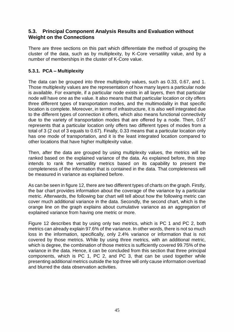
45

5.3. Principal Component Analysis Results and Evaluation without Weight on the Connections There are three sections on this part which differentiate the method of grouping the cluster of the data, such as by multiplexity, by K-Core versatility value, and by a number of memberships in the cluster of K-Core value.

5.3.1. PCA – Multiplexity The data can be grouped into three multiplexity values, such as 0.33, 0.67, and 1. Those multiplexity values are the representation of how many layers a particular node is available. For example, if a particular node exists in all layers, then that particular node will have one as the value. It also means that that particular location or city offers three different types of transportation modes, and the multimodality in that specific location is complete. Moreover, in terms of infrastructure, it is also well integrated due to the different types of connection it offers, which also means functional connectivity due to the variety of transportation modes that are offered by a node. Then, 0.67 represents that a particular location only offers two different types of modes from a total of 3 (2 out of 3 equals to 0.67). Finally, 0.33 means that a particular location only has one mode of transportation, and it is the least integrated location compared to other locations that have higher multiplexity value. Then, after the data are grouped by using multiplexity values, the metrics will be ranked based on the explained variance of the data. As explained before, this step intends to rank the versatility metrics based on its capability to present the completeness of the information that is contained in the data. That completeness will be measured in variance as explained before. As can be seen in figure 12, there are two different types of charts on the graph. Firstly, the bar chart provides information about the coverage of the variance by a particular metric. Afterwards, the following bar chart will tell about how the following metric can cover much additional variance in the data. Secondly, the second chart, which is the orange line on the graph explains about cumulative variance as an aggregation of explained variance from having one metric or more. Figure 12 describes that by using only two metrics, which is PC 1 and PC 2, both metrics can already explain 97.6% of the variance. In other words, there is not so much loss in the information, specifically, only 2.4% variance or information that is not covered by those metrics. While by using three metrics, with an additional metric, which is degree, the combination of those metrics is sufficiently covered 99.75% of the variance in the data. Hence, it can be concluded from this section that three principal components, which is PC 1, PC 2, and PC 3, that can be used together while presenting additional metrics outside the top three will only cause information overload and blurred the data observation activities.

46

Figure 12. The rank of Metrics based on Explained Variance – Clustering by Multiplexity

The next step is to visualize and observe the cluster of the data by plotting it into 2D axis that consists of PC 1 as the x-axis and PC 2 in the y-axis. By plotting the data into a 2D axis with those axes, the dispersion of the data, and how the data is clustered together can be observed. Four plots are presented below. Different colours can differentiate the clusters. In other words, different colours visualize different groups. One plot visualizes all of the clusters together. Then, the other three plots below only activated two clusters in the cartesian coordinate to see the differentiation between clusters more clearly. As can be seen in the plots below, to group the data by using multiplexity, there is still some overlap between groups. Hence, two crucial points can be noticed from this observation. Firstly, it cannot be concluded the tendency of versatility by multiplexity. It cannot be concluded that the ports that have high multiplexity have a high versatility or more central role in the network. However, it can be observed that the most central ports on the network (Rotterdam, Antwerp, Hamburg, and Bremerhaven), all of them have multiplexity of 1. However, it does not necessarily mean that the ports that have three modal connection also have a high versatility. The reverse causation is not valid in this case. Secondly, multiplexity is not an excellent variable to group the data due to the overlap and unclear boundary between clusters. However, both principal components are good metrics to present all range of the data and variances in the data as can be seen on the four plots below.

47

Figure 13. Scatter Plot of Data with PC 1 and PC 2 as the axis (three multiplexity are presented)

Figure 14. Scatter Plot of Data with PC 1 and PC 2 as the axis (two multiplexity are presented – 0.33 and 0.67)

48

Figure 15. Scatter Plot of Data with PC 1 and PC 2 as the axis (three multiplexity are presented – 0.33 and 1)


49

5.3.2. PCA – Top K-Core Previous PCA analysis was deemed not sufficient to present the classification of the data due to the overlapped between groups. Hence, this section and the next section utilizes K-Core value to group the data. The difference between this section and the following section is this section will group the data based on the top K-Core value, while the next section will group the data based on the number of members of K-Core clusters. The intention of grouping by several members of K-Core clusters will be explained in the following section. The step is very similar to the previous section. From figure 17, it can be determined that by using only one principal component which is PC 1, it is sufficient to describe 84.45% variance in the data, while using two and three principal components can describe 93.35% and 99.56% variance of the data. Then, it can be understood by only use two metrics, which is PC 1 and PC 2; both of them can explain 93.35% of the variance without losing too much information. However, by using three metrics, with degree metric as an additional metric, can describe 99.56% of the variance. Hence, based on the explanation above, it can be concluded that using three principal components consisting of PC 1, PC 2, and PC 3 can describe most of the information on the data. This result is the same as a result of the previous section.

Figure 17. The rank of Metrics based on Explained Variance – Clustering by 5 Highest K-Core Value

Figure 18 and figure 19 shows the clustering of the data based on the 5 highest K-Core value, which is 38, 36, 34, 33, 32. The colours differentiate the clustering of the data. The explanation of K-Core has been explained in chapter three. To summarize, the higher K-Core value, the more central a node is. In short, K-Core represents connected core areas in the network (IBM, 2016). As a member of a certain K-Core, a node needs to be connected with a minimum number of k other entities in the network (IBM, 2016).

50

Based on the result below, the K-Core does not go in parallel with the outcome of PC1 and PC2. The highest K-Core, which is 38, does not necessarily have a high PC1 and PC2. It is because K-Core is only a versatility metric in a multilayer network that provides information about “boundary” to join a specific community. However, the more suitable approach to determine the significance or versatility of a node is by evaluating how influential the node is. In this case, a node is more prominent or has a more central role if a node is referred to by other nodes that have a more central role as well. This context has been well-described by PC1 and PC2, which is the first and second principal component metrics. Then, the K-Core value can be used only to group the data. Although there is still some overlap between cluster, grouping by highest top five K-Core values has improved the visualization as can be seen in figure 19. In figure 19, the clustering between different K-Core values can be differentiated. Both principal component one (PC 1) and principal component two (PC 2) can distinguish the cluster well and exhibit most of the variance in the data.

Figure 18. Scatter Plot of Data with PC 1 and PC 2 as the axis (Full Clusters are presented)

51

Figure 19. Scatter Plot of Data with PC 1 and PC 2 as the axis (4 clusters are presented – 36 is not presented)

5.3.3. PCA – K-Core Members The previous analysis is still shown some overlap due to the narrow range of versatility value. Hence, some stacked up in the data needs to be expected. In this section, the plot will be ranked based on the number of members in a particular K-Core value. It was expected to have a more extensive range of K-Core value as a representation of versatility. Then, the steps will follow the steps in previous sections. In this section, the chart of explained variance will not be shown it was expected the chart would be the same chart. Both of these sections (previous section and this section) grouped the data based on K-Core value. Hence, the explained variance in the data for both sections will be based on the same range of K-Core value and present the same data clusters if all clusters will be plotted. The difference will be visualized in the next two visualizations below. Figure 20 shows all clusters in the cartesian coordinate (the axes are PC 1 and PC 2). The graph shows the top ten clusters with most members. Moreover, as can be seen below, it presents a more comprehensive range of K-Core value, starting from 2 to 36. However, some data overlapped is still existed, specifically for a close K-Core value, such as 2, 4, 6, 8, 10, and 12. It is the same issue as the issue in the previous section. Figure 21 will be presented to overcome this issue and provide clarity to the visualization and analysis. Figure 21 shows five different classes, which are in a broader range of value, from low (2, 4, 6), mid (22), and high (36) K-Core value. From figure 21, the classes can be differentiated from each other by utilizing principal component one (PC 1). Principal component two (PC 2) provides more information about the variance in the data and add the completeness in the information. However, PC 1 is sufficient to differentiate the data. Then, it can be concluded that based on the trend or separation of clusters by using PC 1, the higher the K-Core value which means the clusters play a more central role in the network, the higher the PC 1 value

52

is. In other words, the more influential or, the more versatile the clusters are, then the higher the PC 1 value is. Hence, PageRank is the right choice of metric to rank the versatility of the clusters or the nodes.

Figure 20. Scatter Plot of Data with PC 1 and PC 2 as the axis (all clusters)

Figure 21. Scatter Plot of Data with PC 1 and PC 2 as the axis (5 clusters are presented – 2,4,6,22,36)

53

5.4. Principal Component Analysis Results and Evaluation with Weighted Connections This section will take weight in each connection between nodes into account. The method to quantify the weight of the links has been explained in chapter 3. Then, the rest of the sections will be similar to the previous three sub-sections. This section will start by using multiplexity to do a grouping of the data that are followed by grouping by K-Core values.

5.4.1. PCA – Multiplexity While the steps and types of visualizations have a similar type, the difference is there is one additional metric in weighted connection. That metric is a strength. Strength is essentially similar to a degree. The algorithm and mathematical formulation of strength are the same as degree as can be seen in chapter three. However, instead of just aggregating the value of incoming and outgoing connection, strength takes weight in each connection into consideration. Figure 22 shows virtually the same type of information, as explained in the previous section. Hence, the explanation will not be repeated. From figure 22, three top metrics explained most of the variance in the data, which is PC 1, PC 2, and PC 3. There is a drop in each incremental of the principal component. It is because of the overlap in the information. Figure 22 provides information on both individual contributions of the metrics and cumulative contributions, as explained in the previous section as well. By only utilizing PC 1 as the versatility metric, it can explain about 72.52%, while by adding PC 2 to describe the data, it can add 19.26% of the explained variance with a cumulative explained variance of 91.78%. Then, by adding the PC 3 and utilizing three metrics to describe the data, it can explain 98.94% of the explained variance in the data without losing too much information. Then, the rest of the metrics can be removed safely.

Figure 22. The rank of Metrics based on Explained Variance – Clustering by Multiplexity

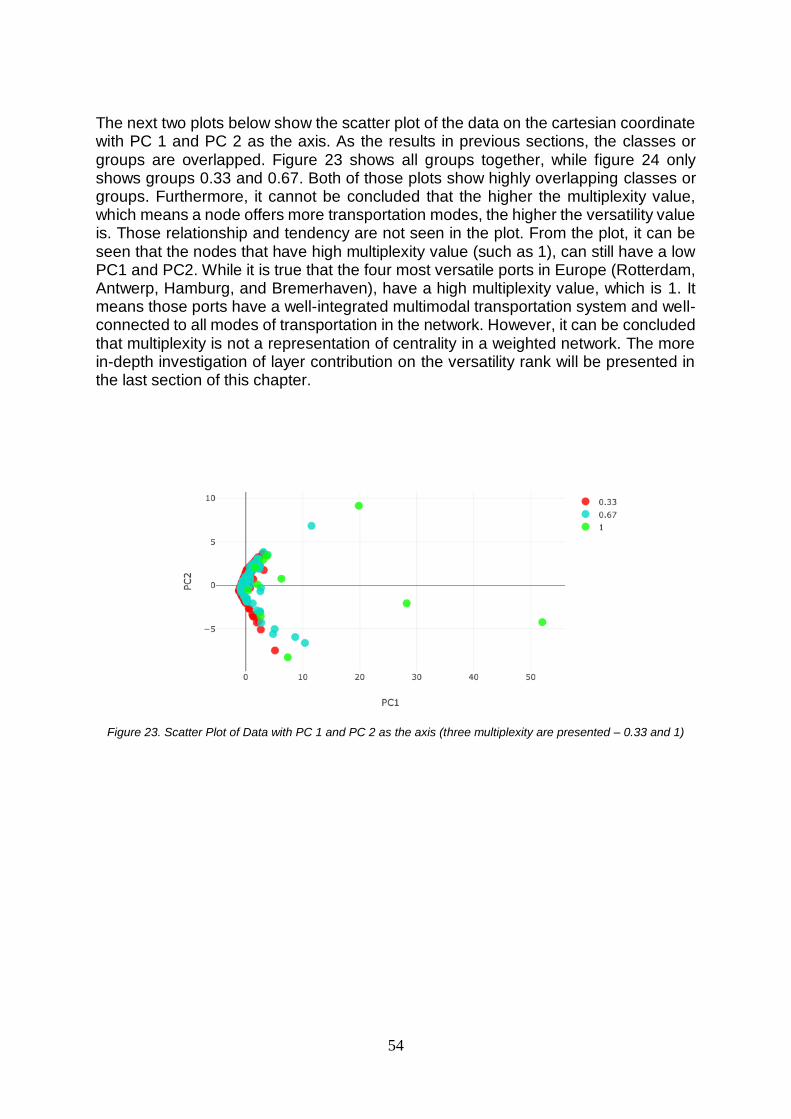
54

The next two plots below show the scatter plot of the data on the cartesian coordinate with PC 1 and PC 2 as the axis. As the results in previous sections, the classes or groups are overlapped. Figure 23 shows all groups together, while figure 24 only shows groups 0.33 and 0.67. Both of those plots show highly overlapping classes or groups. Furthermore, it cannot be concluded that the higher the multiplexity value, which means a node offers more transportation modes, the higher the versatility value is. Those relationship and tendency are not seen in the plot. From the plot, it can be seen that the nodes that have high multiplexity value (such as 1), can still have a low PC1 and PC2. While it is true that the four most versatile ports in Europe (Rotterdam, Antwerp, Hamburg, and Bremerhaven), have a high multiplexity value, which is 1. It means those ports have a well-integrated multimodal transportation system and well-connected to all modes of transportation in the network. However, it can be concluded that multiplexity is not a representation of centrality in a weighted network. The more in-depth investigation of layer contribution on the versatility rank will be presented in the last section of this chapter.


55

Figure 24. Scatter Plot of Data with PC 1 and PC 2 as the axis (two multiplexity are presented – 0.33 and 0.67)

5.4.2. PCA – Top K-Core The results explanation will be mainly the same as the previous sections. Hence, to be not repetitive, it will be made more straightforward in the following explanation. From figure 25, it can be determined by using four versatility metrics consisting of PC 1, PC 2, PC 3, and PC 4. It can explain 99.71% of the variance in the data with a 0.29% loss in the information only. If three metrics that are consisting of PC 1, PC 2, and PC 3 only were used, then the cumulative explained variance is about 96.15%, which is still very high. However, it can be decided that by using the four highest principal components will be the best option, and the rest of the metrics can be safely removed.

Figure 25. The rank of Metrics based on Explained Variance – Clustering by 5 Highest K-Core Value

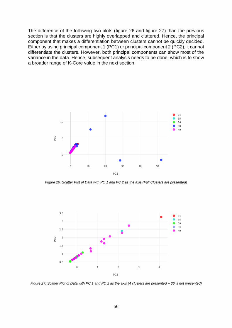
56

The difference of the following two plots (figure 26 and figure 27) than the previous section is that the clusters are highly overlapped and cluttered. Hence, the principal component that makes a differentiation between clusters cannot be quickly decided. Either by using principal component 1 (PC1) or principal component 2 (PC2), it cannot differentiate the clusters. However, both principal components can show most of the variance in the data. Hence, subsequent analysis needs to be done, which is to show a broader range of K-Core value in the next section.

Figure 26. Scatter Plot of Data with PC 1 and PC 2 as the axis (Full Clusters are presented)


57

5.4.3. PCA – K-Core Members The following two plots have the objective to complement the analysis of the previous section by showing a more comprehensive range of K-Core value. Figure 28 shows the top ten K-Core value based on the number of members in each K-Core class or group. While figure 28 still has cluttered information, figure 29 only shows four K-Core classes (classes 4, 10, 24, 38). According to figure 29, principal component two is a good metric to see the separation between clusters vertically. With an additional metric which is PC 1, it can explain most of the variance of the data as explained before. From this section, it can be concluded that the data can be grouped by K-Core value. Then, the combination of four metrics consisting of PC 1, PC 2, PC 3, and PC 4 can be used to analyze the next step to have an aggregated ranking which is a consensus rank from the different metric. That method is called the Borda count. However, the disadvantages of the result from this section are the relationship between PC 1 and PC 2 versatility with K-Core versatility measure is not clear due to the trend and tendency of the clusters based on its placement on the cartesian coordinate cannot be easily determined.


58

Figure 29. Scatter Plot of Data with PageRank and Eigenvector as the axis (5 clusters are presented –

2,4,6,22,36)

5.5. The Disadvantages of Principal Component Analysis As shown from previous analysis, the principal component analysis is very useful unsupervised learning algorithm for dimensional reduction. However, it is challenging to understand what a particular principal component represents. As it can be seen from the analysis, the principal component does not specifically represent a single metric (such as PageRank or Eigenvector). On the other hand, the principal component consists of a combination of several metrics that have been defined earlier. Therefore, before continuing to the next analysis. This section will break down the components based on the grouping of the K-Core. From K-Core section, by referring to figure 30, it can be understood that 2 principal components can explain 90% variance of the data. Hence, figure 30 below is the breakdown of each principal component.

59

Figure 30. The Breakdown of The Contribution of Each Metric in PC 1 and PC 2 (Top K-Core Grouping)

Figure 30 represents the contribution of each metric in principal component 1 and 2. In other words, the number provides information about the correlation of each parameter to the principal component itself. The higher the number, then the bigger the contribution of the metric to the principal component. In principal component 1, it can be seen that the PageRank, Strength (including StrengthIn and StrengthOut because it is highly correlated), and degree have a high contribution to PC 1. While in principal component 2 (PC 2), it can be seen that Eigenvector, Degree (including DegreeIn and DegreeOut because it is highly correlated and basically DegreeIn and DegreeOut is the building blocks of degree), hub, authority, and Katz have a high contribution to PC 2. However, for simplification and dimensional reduction for the next section, only the base metric that will be used in the next section. In this case, hub, authority, and Katz are the derivatives of Eigenvector. Hence, Eigenvector will be used as the representation of that information. Additionally, the same reasoning will be used for Degree and Strength. Therefore, for the next analysis, there are four components for Borda count which is PageRank, Eigenvector, Degree, and Strength.

60

5.6. Constructing the Ranking of European Hinterland Hubs Previous sections presented the result from the network which has no weight assigned on the connections and the network with weight on the link connection. It is decided that the weighted connection will closer to represent the reality since, in the practicality of the multimodal network, each connection may have a different capacity and attractiveness, which depends on the demand of a particular location. Hence, the focus will be shifted into the result from the section of weighted connection. From earlier section, it can be summarized that multiplexity is not a good indicator to group the data. Hence, the results from K-Core section is more relevant to be processed for the next step. In K-Core section, four metrics can be used to present most of the variance of the data with only a little loss in information. Those metrics are PageRank, Eigenvector, Strength, and Degree. Then, each of those metrics will be used to form an aggregated ranking based on ranking consensus from each metric. For example, each metric can be utilized to rank the hubs. Then, the rank of a hub in one metric can be different from other metrics. The difference should not be too far, in any case. Afterwards, the rank of a hub from each metric can be aggregated into a single number. The hub that has the smallest value has a higher rank. This method is called Borda count and often used as a preference-based ranking method in policy analysis. The result of the aggregated rank can be seen in table 3 below. Table 3 shows that Rotterdam is the most versatile ports all over Europe, followed by Antwerp, Hamburg, Bremerhaven, and Valencia. This rank has already taken multiple types of transportation across layers and also combining different metrics in the process. Furthermore, the next process is to construct a new network that is focusing on those twelve hubs as origins and destinations. Then, the layer that has the most significant contribution to the rank can be determined, and additional network diagnostics and measures can also be performed that act as a foundation to subsequent analysis.

61

Rank Port Name Borda Count

1 Rotterdam 6

2 Antwerp 10

3 Hamburg 16

4 Bremerhaven 21

5 Valencia 24

6 Piraeus 28

7 Felixstowe 36

8 Le Havre 38

9 Barcelona 39

10 Algeciras 40

11 Marsaxlokk 41

12 Southampton 53

13 Gioia Tauro 58

14 Gdansk 61 Table 3. Rank of The Container Hubs based on Versatility

5.7. Contribution of Hinterland Multilayer Network Structure to Versatility Rank This section will do an investigation of the versatility rank of the European hinterland network. This section will present the full weighted network structure layer by layer. The network focuses on twelve most versatile hubs as point-of-origins and destinations with the connections between nodes. However, before going into the investigation of the full network, a brief explanation about the ranking system and distribution of the weight of the connections will be presented first to have a general understanding of the ranking mechanism. As explained in chapter three, the ranking mechanism in the multilayer network is based on a consensus of the ranking in every layer as a simplification to be able to understand the method. The consensus of the ranking in every layer can be done in three ways, such as each layer has the same weight, weighted by links, or weighted by node (De Domenico, Solé-Ribalta, Omodei, Gómez, & Arenas, 2015). In this study and the algorithm implemented in Muxviz, every layer has the same weight. The more detail of explanation of the ranking mechanism in this study is that Muxviz utilizes a tensorial approach to evaluate the rank. This tensorial approach is based on a random walker to evaluate the versatility of a node by moving throughout the network and inspect the connections on a particular node on the network where figure 31 describes it more straightforwardly (De Domenico et al., 2015). Then, the algorithm will rank the centrality of the nodes by aggregating the results from every node. Figure 31 shows an edge-coloured network where it will provide a more straightforward example compared to a node-coloured network (interconnected network). As explained in chapter three, the edge-coloured network only has interlayer connections

62

for the same node in every layer. The random walker can move from one layer to another layer by using those nodes as a transfer location or a transfer point or a “hub”. Then, from this explanation, the nodes that have “central” role will act as a “bridge” that connects to other influential nodes on different layers (De Domenico et al., 2015).

Figure 31. The Interpretation of Random Walkers Movement in Multilayer Network to Determine Versatility Rank

(Edge-Coloured Network) (De Domenico, Solé-Ribalta, et al., 2015)

In edge-coloured network, the interlayer links which connect the same nodes in every layer have a weight as well. Then, in this case, it is crucial to know the distribution of the weight of the connections in the network before assigning the proper weight for the interlayer connections. Figure 32 shows the distribution of the weight of the connections. From that figure, it can be seen that the distribution is skewed to the right. It is caused by a major hub which located on the right of the distribution that has a high degree and strength of the connections relative to other locations, such as Rotterdam, Antwerp, Bremerhaven, and Hamburg. Because of the form of the distribution, then it was decided to have the median value assigned as the interlayer weight. The reasoning is because the mean value is affected by the value of the outliers that are located on the right part of the distribution. Hence, the mean value will also be shifted to the right. However, the median value is more neutral because it is not affected by the outliers on the right side of the distribution. In this case, the value of the interlayer connection is, which is also the value of the median of the overall network.

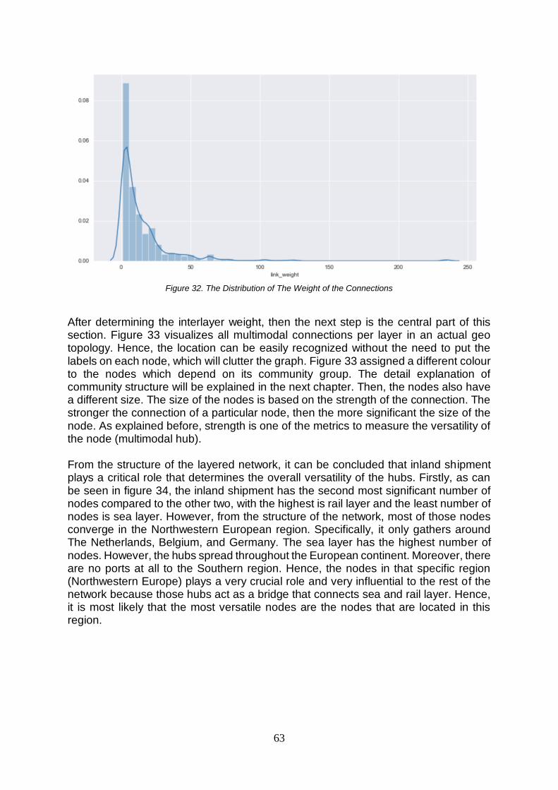
63

Figure 32. The Distribution of The Weight of the Connections

After determining the interlayer weight, then the next step is the central part of this section. Figure 33 visualizes all multimodal connections per layer in an actual geo topology. Hence, the location can be easily recognized without the need to put the labels on each node, which will clutter the graph. Figure 33 assigned a different colour to the nodes which depend on its community group. The detail explanation of community structure will be explained in the next chapter. Then, the nodes also have a different size. The size of the nodes is based on the strength of the connection. The stronger the connection of a particular node, then the more significant the size of the node. As explained before, strength is one of the metrics to measure the versatility of the node (multimodal hub). From the structure of the layered network, it can be concluded that inland shipment plays a critical role that determines the overall versatility of the hubs. Firstly, as can be seen in figure 34, the inland shipment has the second most significant number of nodes compared to the other two, with the highest is rail layer and the least number of nodes is sea layer. However, from the structure of the network, most of those nodes converge in the Northwestern European region. Specifically, it only gathers around The Netherlands, Belgium, and Germany. The sea layer has the highest number of nodes. However, the hubs spread throughout the European continent. Moreover, there are no ports at all to the Southern region. Hence, the nodes in that specific region (Northwestern Europe) plays a very crucial role and very influential to the rest of the network because those hubs act as a bridge that connects sea and rail layer. Hence, it is most likely that the most versatile nodes are the nodes that are located in this region.

64

Furthermore, the second most contributor is sea layer. Because as can be observed from figure 35, the sea layer has the highest density compared to other layers. Density, in this case, is the ratio between edges and nodes. The higher the density, the more edges each node will have. Hence, each node has a higher importance, which causes a higher versatility rank. Because every node that has a connection with a node with more edges, it will have a higher PageRank and Eigenvector value. Hence, the position in the network is more important and critical.

Figure 33. The European Multimodal Hinterland Network with Weighted Connections

Figure 34. Node Counts in Each Layer

65

Figure 35. Density of the Network per Layer

5.8. Chapter Summary and Conclusion To sum up this chapter, there are several points of observations and analysis that can be concluded. Firstly, the weighted network is the best way to represent the multimodal network because of its actual representation of the network. Weighted connections deliver the information, such as the importance of the links because, in actual connection, every link has a different attractiveness, capacity, and trade movements. Secondly, K-Core is a good measure to cluster the data compared to multiplexity. While on a weighted network, some overlapped happened. In the unweighted network, K-Core can give clear representation that differentiates different cluster based on centrality. Then, there is a tendency of the groups that play a more central role, has a higher PageRank and Eigenvector value. Both PageRank and Eigenvector represent preferential attachment to a more influential node. Thirdly, four principal components can describe most variance on the data as presented in the analysis, such as PageRank, Eigenvector, Degree, and Strength. Then, the combination of those metrics resulted in the European most important hubs. Fourthly, based on the network structure, inland shipping layer is the crucial layer that determines the centrality of the node because of that layer bridge or builds a connection to other layers which is sea layer and rail layer. Sea layer is one of the most significant contributors to the versatility rank due to the density of the layer. It has the highest number of edges per node. Because the container hubs are accumulated in the Northwestern region of Europe in inland shipping layer, then the most versatile node in the network can be found there. It can be concluded that Rotterdam, Antwerp, Bremerhaven, and Hamburg are the most critical node in the network.

66

The next section will inspect the community structure of the network. In the next section, the criticality of each community structure will be investigated. Then, those analyses will be complemented with cooperation and connectivity analysis in chapter 8, which act as a foundation for robustness analysis in the last chapter.

67

Chapter 6: The Community Structure of the European Multimodal Transportation Network

6.1. Introduction The previous chapter has identified the twelve most versatile hubs in European multimodal network. This chapter will continue the analysis by focusing on those twelve hubs as origins and destinations. Those twelve hubs are scattered around European regions, such as Northern and Southern part of Europe. Then, the identification of groups of ports that shape a certain community will be executed and explained. The initial analysis about community detection will serve as a foundation to the following sections, which is more to the operational analysis of the transportation network itself. Once the communities have been identified, the analysis will continue with the investigation of Matthew Effect in the European multimodal transportation network. This analysis intends to observe and analyze the inequality between communities. Furthermore, the last two investigations about the evolution of interlayer communities and level of integration per community will serve as a foundation of criticality analysis, which concludes all analysis in this chapter.

6.2. Community Detection in the European Hinterland Transportation Network

The first step in this section is to divide the full network into several communities based on the Multiplex Infomap algorithm. This algorithm is built on a fundamental algorithm, which is called the map equation (M Rosvall et al., 2010). Then, this algorithm was extended to be applied to community detection in a multilayer network. As explained in chapter three, Multiplex Infomap detects communities in multiplex network structure. To say it briefly, Multiplex Infomap identifies communities in a network based on the information flow inside the network. The base algorithm is based on a random walker that moves inside the network. Then, the probabilities of the movement are proportional to the weights of the connections between nodes and layers (Domenico et al., 2015). This section will present the result of community detection as a foundation for the following sections. The following sections will be more to the operational parameter of the transportation network itself, which will lead to the criticality analysis, to sum up, every section. The network that was explored in this analysis is the edge-coloured and directed network with weighted connections. As explained in the previous chapter, the network that would be investigated is directed and weighted because it is more representative to describe the practice in the real world since each chain in the real world has a particular attractiveness, capacity, and direction (from source to destination). The community discovery in an edge-coloured, weighted, directed, and the layered network is represented by figure 36 and figure 37. This network is focused on twelve hubs that have been defined in the previous chapter as origins and destinations. Community discover in a multilayer network depends on the relax rate. As explained

68

earlier, the relax rate is a probability that allows the random walker to move to other layers and continue the community detection process there. The community that has the same identification number, although it is located in other layers, it is part of the same community. For example, community number three in sea layer and community three in rail layer will show the same community and the same groups or clusters of ports. Three crucial figures set the foundation for the next analysis. Those figures are figure 36, 37, and 38. Those figures intend to show the process of determining the relax rate that set as a fundamental component that will be used in the following sections. There are two subfigures in figure 36. The figure on the left shows the relationship between the number of communities that are discovered and relax rate. Then, the picture on the right explains the code length and relax rate. The code length is often called a variable-length code. Variable-length code is a code that is used to do compression and decompression of data. The lower the value of the code length, then the computer needs lower resources to compress or decompress a source data. This technical detail is a least of importance in the context of multimodal network analysis. However, it will be insightful to observe the trend of the code length on different relax rate. The trend that will be useful is when the code length will converge to stability. Moreover, the subfigure on the left of figure 36 is relatively straightforward to interpret. As stated earlier, it is a relation between the number of communities that are discovered and relax rate. The lower the relax rate, then the less likely the random walker moves to other layers to continue the community discovery there. Hence, community detection is bounded to a specific layer. As a result, more independent communities are discovered, which lead to a higher number of community identification. Then, if the relax rate is released into a higher value, the random walker is easier to move to other layers to continue the community detection. Hence, it is more likely to find some nodes or ports are the members of the same community, although they are located in different layers. That kind of situation leads to a lower number of communities as can be observed from the graph. Figure 37 describes the morphology of how some nodes merged to other parts of communities when the relax rate changes. The different colours of the chart identify different identification of community structure. The figure is also relatively straightforward to interpret since the morphology is clearly visualized there. However, some micro-information will not be able to be presented that will clutter the visualization. The micro-information that was not presented is the detail information of the name of the ports that are joined other communities. However, the objective of figure 37 is to present a stable relax rate when the communities stop merging and converge to a fixed number of communities. Both figure 36 and 37 have the same objective which is to present the stable point or relax rate when no more communities are merged. Then, set a particular relax rate that will be used for community identification. In this case, the relax rate of choice is 0.604 because it is the stable point where no more changes in the community structure as figure 37 shows. Moreover, the communities have merged into five communities in total across layers.

69

Figure 38 provides deeper information once a particular relax rate, which is 0.604, has been chosen. Figure 38 intends to show the number of community identification per layer. This figure can answer a question, such as “if there are five communities in total, how many communities can be identified in a particular layer? Do all layers have the same number of communities?” Figure 38 shows different colours coding for various layers, such as dark blue for sea layer (number one), light blue for the inland layer (number two), and orange for rail layer (number three). The y-axis describes several nodes per layer, while the x-axis shows the numbering of community identification. Hence, from figure 38, it can be known that there are five communities in total. More specifically, five communities were identified in the sea layer, two communities were identified in the inland layer, and five communities were found in rail layer. In the case of rail layer, five communities are defined in the layer. However, specifically for community number five in rail layer, there is only one port, which is Istanbul. This is because Istanbul was identified as community member number five in the sea layer. To conclude this section, the relax rate that was chosen is 0.604, which leads to five communities in total across layers. As additional information for subsequent analysis, since there is only one port city that was detected in rail transportation layer and it is not the part of twelve most versatile hubs, there are only four communities that will be considered in rail transportation. The reasoning is because the clusters should work together, and it cannot stand on themselves alone. Moreover, the role of Istanbul in the network is not entirely ignored since Istanbul will take into account as a member of community member number five in the sea layer. Then, Istanbul should ideally part of two different communities, which is part of community number five in sea layer (part of Southeast European region from Italy to Turkey) and a part of community number one in rail layer (part of the same community as Rotterdam) considering its shipping network and schedule. This can be tweaked easily from the community table. However, considering its size and remote geographical location in the rail network, the impact of Istanbul is of least significance and does not affect the statistical measurement of overall network.

Figure 36. Communities Discovery and Relax Rate

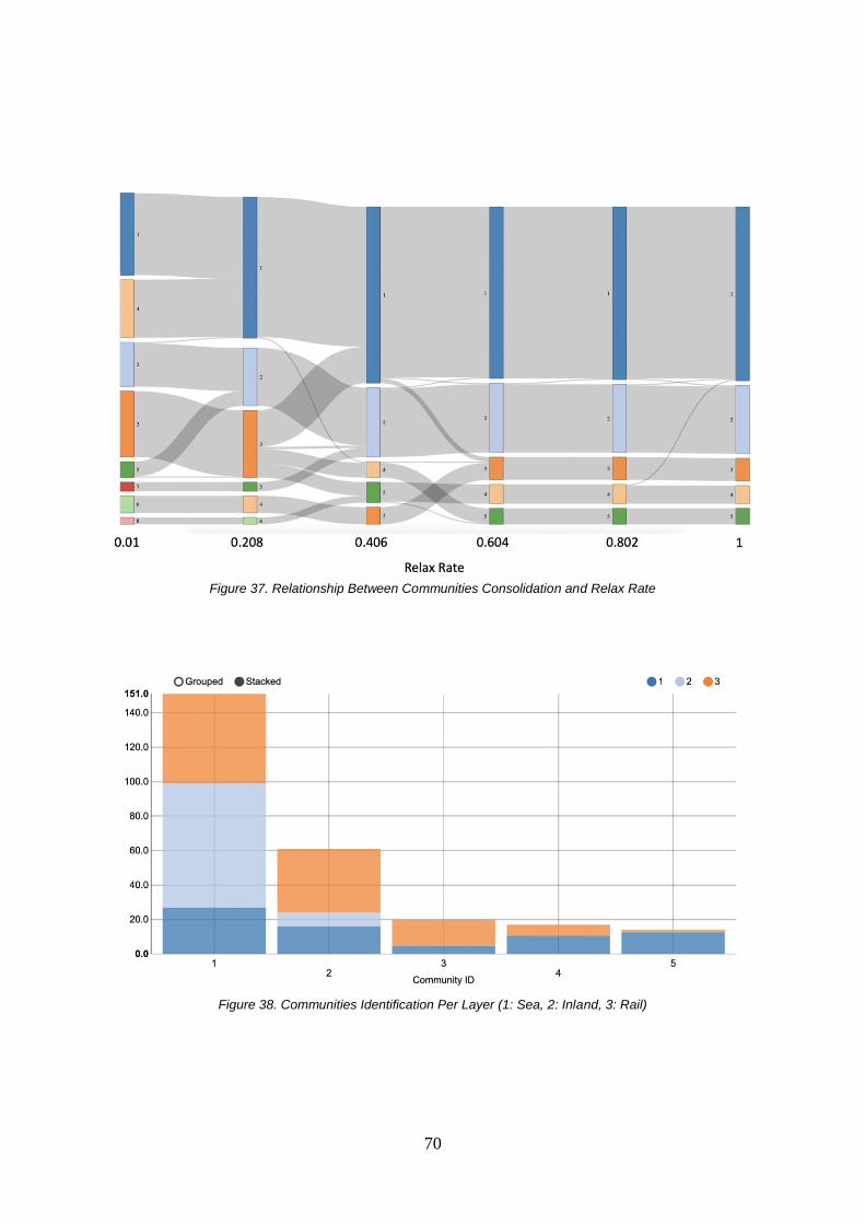
70

Figure 37. Relationship Between Communities Consolidation and Relax Rate

Figure 38. Communities Identification Per Layer (1: Sea, 2: Inland, 3: Rail)

71

6.3. The Community Structure of the European Hinterland Transportation Network

This section will elaborate more detail information of community structures in EHTN. By using relax rate of 0.604, the total of five communities exists in the network. However, different layers may present different communities’ coverage. Not all communities will present in a particular layer since it depends on the reach of the shipping network in a specific layer and geographical service area of a particular community in a specific layer. For example, as figure 39 shows, the sea layer has the furthest extent and geographical reach. Moreover, the sea layer network is also the most extensive network compared to all existing layers. Extensive here means it has more connections or link options from a particular node. Hence, it has more possible routes offered compared to other layer’s networks. That extensiveness translates to the density of the network of sea layer as stated in the chapter about versatility. As a reminder, density is more edges per node. The more extensive a network is the more communities that can be found on that layer. The reasoning is because the extensiveness of the network transcribed to more possible options of preferred connections. As a result, more hubs form a particular community structure by following the scale-free structure or preferential attachment. Due to more options of preferred connections, it translates to a smaller diameter of a particular network. Then, it leads to the more possible identification of different communities due to the relative closeness of the network or smaller network diameter. In this case, the sea network has the smallest diameter of all, followed by the rail network. Afterwards, the inland transportation network has the largest diameter. The graph can be seen in figure 39 concerning the network diameter. Hence, based on the earlier argument, the inland layer should have the lowest number of communities as will be shown later and the sea network should have the greatest number of communities. The explanations translate into visualisations of figure 40 and 41. Figure 39 shows that sea network has the most extensive geographical coverage which covers the south-western European region (Spain and Portugal) and the southeastern European region (Italy to Turkey). Five distinct communities can be identified in the sea layer network. Moreover, due to the extensiveness of the network and geographical coverage, the southern European region in the sea network can be divided into two distinct communities. The development of the differentiation of the Southern European part started in 2018. The development of the new community in Southern Europe will be elaborated in the next sections, including the impact to the existing community. However, from the figure 40 itself, the distinction of different communities in sea network is not visible as a result of overlapping nodes that are part of other communities in the network. Hence, figure 41 presents the cleaner visualization of the communities with the circle to emphasize a particular community. While the sea network has presented five different communities, the inland network has only two distinct communities due to its narrower geographical coverage. The geographical coverage only extends through all regions in The Netherlands, and only cover a part of Germany and France. Moreover, in terms of network diameter, the inland network has the greatest diameter compared to the other two layers, inversely proportional to its geographical reach. The scientific definition of the network diameter

72

itself is the maximum shortest path length between a source and a destination (Jian & Guan, 2016). Hence, it can be implied that the inland network has the lowest extensiveness compared to the other two layers. Lower extensiveness of the network translates to lower density and fewer options of routing choices. Another reasoning that relates to the lower route choices and extensiveness of the inland transportation network is the geographical limitation of the inland transportation structure. Inland transportation network uses existing natural rivers instead of utilizing man-made rivers which will be extremely costly to develop. Then, there are other natural boundaries of the inland network which further complicates the development of the inland network, such as width and depth of the river. Hence, the existing route options are not so many and limited since the beginning. In other words, inland transportation network has lower flexibility of infrastructure development, which leads to fewer route choices due to fewer incentives for existing actors to invest in it. On the other hand, the sea network and rail transportation network have more flexibility in terms of infrastructure development. Furthermore, both of those networks have more extensive and further geographical reach which connects most of the most versatile hubs in general European region. Hence, most of the actors and authorities have more incentives to further develop sea and rail transportation network, which already have broader reach earlier. Moreover, the development of the sea and rail network are considered more logical and more cost-effective since it offers greater flexibility (more expansive and scalable) and not really limited by natural boundaries. Furthermore, the rail network has four distinct communities which are shown in figure 40 and 41. While figure 40 integrated the information of shipping network that is visualized by the green line, figure 41 provides clearer visualization that put emphasis on the community clustering of the ports. The intention of figure 40, specifically in the rail network part, is to show that London is part of the community of Spanish ports since Valencia in Spain and London are connected by train, while other British container terminals have no shipping schedules to London based on 2019 data as can be seen on the network construction. By utilizing only figure 41, this kind of information would confuse the analysis since the question why London is part of the community of Spanish ports cannot be answered. Hence, figure 40 and 41 complement each other. There are four different communities in the rail network with British container terminals have a totally separate and independent community due to a geographical structure. Those container terminals are separated by natural boundaries, such as the sea that separates the mainland of Europe and the UK. Hence, the container terminals in the UK have different communities that are marked by purple colour, except for London which has been explained earlier. Then, mainland Europe has a more extensive network which connects each other. There are three other distinct communities in mainland Europe, which could be classified as Dutch port communities, German ports communities, and Spanish or the Southern European port communities. It was named as such due to the largest hubs in the respective communities, with Rotterdam is the largest hub in Dutch communities, Hamburg is for German communities, and Valencia is the biggest port in Southern region. Moreover, the noticeable observation that the rail network only covers northern part of Italian region and does not cover Italian region extensively which gives a room for further development in this region and more to Eastern European parts which cover Turkey region as can be seen on the sea network which is the most extensive network in whole multimodal network.

73

As additional information, some container terminals are marked by red colour. It is because the algorithm did not assign a specific community identification because it has far less weight in terms of shipping connections. In other words, it does not have a strong connection with the hubs in the region compared to other existing terminals. Moreover, from the inland transportation network in figure 40, the red community is geographically separated from green (Dutch) and blue (German) community. While red community can be geographically separated, but not all of the case will be like this case. Some of the ports with no identification due to far smaller size compared to other terminals, it usually connects to bigger hubs for consolidation purpose. This specific case will be presented in the following section about network efficiency and integration. The consolidation itself is for the purpose of achieving economies of scale and has a lower transportation cost.

Figure 39. Network Diameter per Layer in 2019

74

Figure 40. Comprehensive Network Visualization for All Transportation Layer in 2019

Figure 41. The Clusters of Hinterland Network in 2019

75

6.4. Matthew Effect in the European Hinterland Transportation Network While previous section has provided detailed information of the process of community identifications, this section will focus on the descriptive statistics and interpretation of various network-related measurement. There are two main parts in this section, which is related to overall community structure and individual measurement of twelve the most versatile hubs. The first part will present the communities that exist in each network layer starting from 2016 to 2019. Then, the second part will provide the same structure of information for the twelve the most versatile hubs in the European region. The main objective of this section is to present the inequality between communities or hubs. Moreover, another intention of this section is to understand how the preferential attachment of several ports to some hub translates to polarization or disparity between them that can be quantified, in other words, to understand the differentiation of bigger communities or more significant communities or hubs to smaller communities or hubs. The term “Matthew Effect” will be used in this section to show the distinction of bigger communities or hubs compared to smaller communities or hubs. The term of “Matthew Effect” was originated from Robert K. Merton in 1968 to show the accumulation of advantages in many areas of life (Merton, 1968, 1988). The etymology of “Matthew Effect” is originated from the Gospel of St. Matthews which said: “For unto everyone that hath shall be given, and he shall have abundance; but from him that hath not, shall be taken away even that which he hath.” – Matthew 25:29 The summary of his research is the accumulation of advantages for many entities in many different aspects of life. There is a kind of feedback and the causal relationship that further enhance for a greater benefit of several entities (Merton, 1968, 1988). As an example, once an entity has an initial reputation, it is considered more attractive for other entities to connect or link to this particular entity due to the incentives and network effect it offers. Then, this preferential attachment will further enhance the reputation of the “famous” entity which multiplied its initial impact in the first place. This kind of effect is often be called the accumulation of benefits, and also inline to an expression that was popularized by Percy Bysshe Shelley, which said: “the rich get richer and the poor get poorer” (Shelley, 1977). The multimodal transportation network has shown a characteristic which is in line with the behaviour that was explained earlier. The EHTN exhibits preferential attachment and also scale-free network structure. The multimodal container terminals that have a lot of advantages in terms of reputations, infrastructures, operational efficiency, route choices, and shipping frequency exhibit “Matthew Effect” behaviour. Those advantages increase the attractiveness of the versatile hubs that will further enhance its reputation across the network. Then, the other container terminals will prefer or have an incentive to connect to more reputable and bigger hubs in terms of size to achieve economies of scale for consolidation purpose. The following sub-sections will present the findings in four years, starting from 2016 to 2019. As mentioned earlier, the emphasis is to show the inequality between communities, the development of new communities, and polarization between bigger communities and smaller communities.

76

6.5. The Exhibit of Matthew Effect in EHTN’s Communities In this section, the inequality between communities will be shown through three operational measurements, which is through PageRank, mean strength, and also observing the mean multimodality of each community in each layer from 2016 to 2019. The objective of analyzing the PageRank is to see the changes in the domination of certain communities compared to others in the context of preferential attachment. Then, mean strength is a more operational variable since it is directly related to the weighted shipping connections and frequencies, which also implies attractiveness, capacity, or importance of a particular connection or link. Moreover, while the PageRank and mean strength are the types of measurements in the context of versatility, this section will present the mean multimodality of each community as well. Multimodality of a transportation network will also often be called multiplexity in a multilayer context. For a more detailed explanation of multiplexity definition, please refer to the chapter that discusses versatility (chapter five). Figure 42 shows the changes in PageRank value of each community in each transportation layer from 2016 to 2019. Before explaining the graph, the community numbering will be detailed. Community 0 refers to a community which is the “weak” community that was detected due to far less shipping frequencies, which translates to its importance compared to other communities. As explained before, it could also because the ports that are the members of community 0 do not have a frequent shipping schedule or connections to the hubs that are part of much bigger communities, such as community one and above. Hence, it impacts to the importance of the smaller container terminals. Moreover, the ports could also be part of community 0 due to geographically separated to other ports, or the size is far much smaller as the case in inland transportation as mentioned in the previous section. This far less versatile container terminal may connect to the hubs for consolidation purpose as stated before. However, it is still part of community 0 due to the size and importance of the container terminals. Community one is the alliance of Dutch and Belgian ports, and also cover some ports in Northwestern European region, such as some Norwegian and Swedish ports. Community one has an overlap with community two, which also serves the Northwestern European region. The difference is community two includes the German ports and also cover most of the ports in Sweden and Norway to its geographically closer to hubs in German rather than the hubs in community one which is Rotterdam and Antwerp. Hence, in the sea transportation network, most of the container ports in the UK connect to the hubs in community one while some ports in Sweden and Norway have a preferential connection to German hubs due to its relative closeness. Hence, it can be concluded that relatively closer ports will be inclined to part of the same community, which is in line with the first law of geography (Tobler, 1970). Then, community 3 covers the Southern European region, more specifically Spanish ports, community 4 contains the ports in Great Britain, and community 5 refers to the Southeastern European region starting from Italy to Turkey. As can be observed from figure 42, there is no change in the domination of community one and two throughout the year of observation. Community 3 has a jump in its PageRank value due to the significant increase in its shipping frequencies, which reflected in the strength of the connections as figure 43 shows from 2016 to 2017.

77

Then, for the rest of the timeline, the domination is stable except the appearance of a new community, which is community number 5 in 2018. Since there is a development in terms of shipping frequencies in 2017 in Spanish communities and also the appearance of the new community in the Southeastern European region (Italy to Turkey), it implies the development and increase of the demand in the Southern European region. Moreover, it could also be understood as a stronger sub-regional polarization in the European region while the Northwestern European still keep their domination in the overall network. However, the changes in the community development in Southern region can be inferred as the community moves towards more even distribution of the influence of existing hubs (Northwestern communities). The development of the Southern European region may have an impact on existing Northwestern communities and close the inequality gaps between them as can be seen in figure 43. While it hasn’t been visible yet in the PageRank value, the existing communities’ development can be seen in the mean strength development from 2017 to 2018. There is a considerable drop that affects all communities due to the appearance of a new community, which is community number five. Most of the communities were affected by 30% of the previous year’s value. Then, the appearance of the new community also influences all layers of the network due to the interdependence of the interlayer connections. However, with the development of community five, community 1 and two still dominates the overall network, with community 1 has the most influence in the network due to it is considered as the most versatile communities as can be seen in the top PageRank value in the sea and rail network. Considering the gap between the highest value and lowest value in the PageRank and mean strength graph, the inequality is the most visible in the sea and inland community due to the gap between highest and lowest value is broader in those network compared to rail community network which only has around 0.01 gap between communities and 0.02 maximum difference (between lowest and highest value in rail network). On the other hand, the widest gap in sea and inland community spread to 0.05. Furthermore, to complement the analysis, figure 44 shows the mean multiplexity that measures the degree of multimodality per community in each year. The observation implied that there is no significant change in the degree of multimodality, except the appearance of the new community, community number 5 (Southeastern European region). This kind of development is in line with the intention of European integration roadmap and TEN-T investment framework towards more well-distributed and integrated multimodal transportation system.

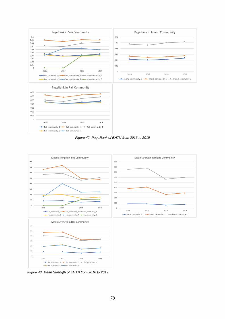
78

Figure 42. PageRank of EHTN from 2016 to 2019

Figure 43. Mean Strength of EHTN from 2016 to 2019

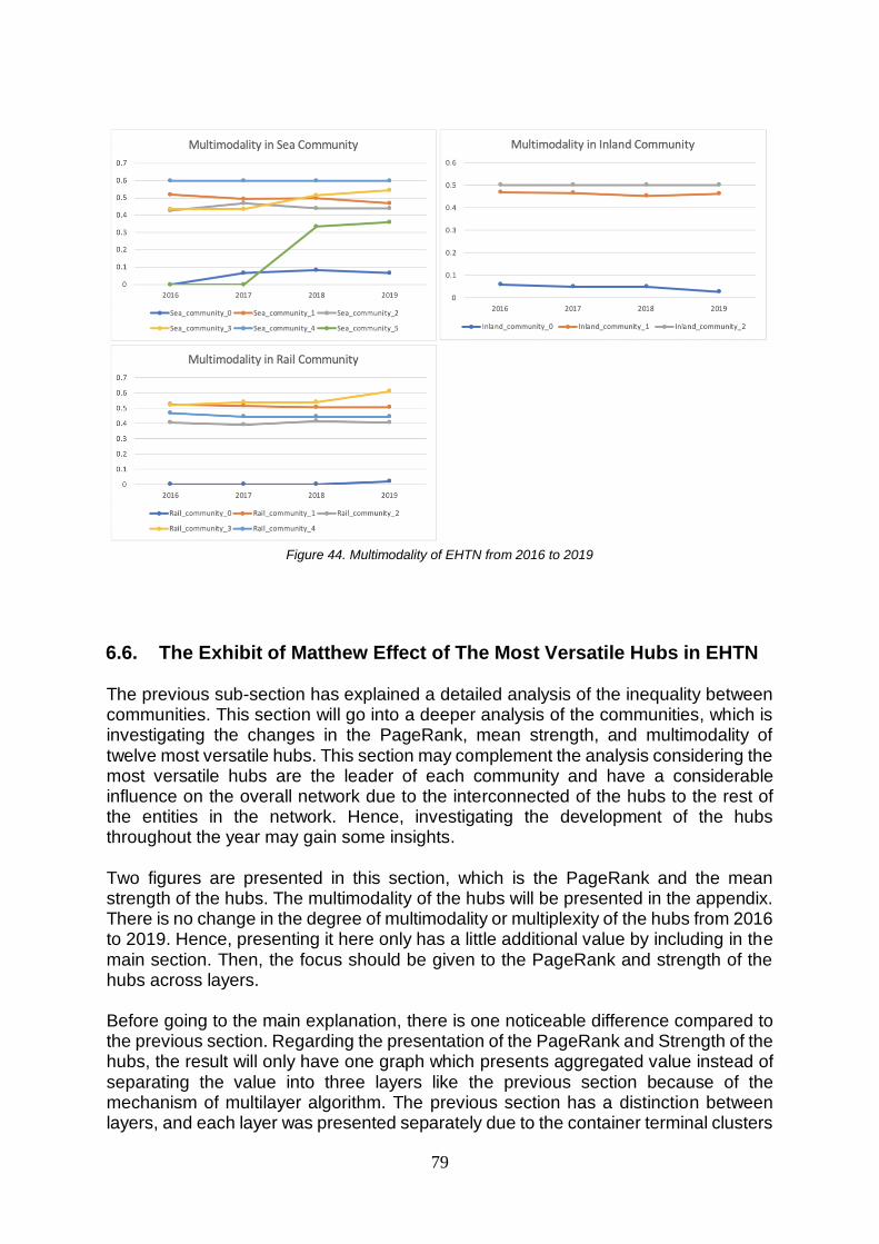
79

Figure 44. Multimodality of EHTN from 2016 to 2019

6.6. The Exhibit of Matthew Effect of The Most Versatile Hubs in EHTN The previous sub-section has explained a detailed analysis of the inequality between communities. This section will go into a deeper analysis of the communities, which is investigating the changes in the PageRank, mean strength, and multimodality of twelve most versatile hubs. This section may complement the analysis considering the most versatile hubs are the leader of each community and have a considerable influence on the overall network due to the interconnected of the hubs to the rest of the entities in the network. Hence, investigating the development of the hubs throughout the year may gain some insights. Two figures are presented in this section, which is the PageRank and the mean strength of the hubs. The multimodality of the hubs will be presented in the appendix. There is no change in the degree of multimodality or multiplexity of the hubs from 2016 to 2019. Hence, presenting it here only has a little additional value by including in the main section. Then, the focus should be given to the PageRank and strength of the hubs across layers. Before going to the main explanation, there is one noticeable difference compared to the previous section. Regarding the presentation of the PageRank and Strength of the hubs, the result will only have one graph which presents aggregated value instead of separating the value into three layers like the previous section because of the mechanism of multilayer algorithm. The previous section has a distinction between layers, and each layer was presented separately due to the container terminal clusters

80

that shape the community structure are different from one layer to other layers due to the transitions of the sub-clusters that happen between layers. This behaviour will be explained in the last section of this chapter and presented in the Sankey diagram. Hence, the same community in the different layer may have different value due to the difference in the sub-clusters that shape the base structure. Therefore, all layers may need to be presented separately. This specific section about the hub is different because the hub is always the same across the layer. Hence, it only has one single PageRank and strength measurement. Figure 45 about the PageRank shows no change in the development of the hubs. The trend is stable, and there is no change in the domination of the hubs or rank of the hubs from 2016 to 2019. However, the PageRank shows a significant gap with 0.9 PageRank unit between the most versatile hub, in this case, is Rotterdam, to the least significant hub, which is Le Havre. Then, from Rotterdam to the second most versatile hub, Hamburg, has a big gap as well, which equal to 0.4 PageRank unit. Those gaps show the inequality in the development of the hubs and one of the proofs of the product or property of the Matthew Effect in the network due to the preferential attachment. However, the development of the new community in the Southeastern European region has a considerable impact on the strength of connections of Rotterdam and other hubs in the overall European region. This is due to the changes or transitions in the shipping schedule and connections of the existing hubs. The new community in Southeastern European region may connect to the versatile hubs that are closer to the region. Then, the rest of the community members may further enhance the connections between them, which multiplied the effect further.

Figure 45. The PageRank of The Most Versatile European Hubs from 2016 to 2019

81

Figure 46. The Mean Strength of The Most Versatile European Hubs from 2016 to 2019

6.7. Efficiency Level in the Communities of European Hinterland Transportation Network

The findings can be grouped into three major parts in this section as represented by figure 47, figure 49, and figure 50. The objective of this section is to present the analysis of integration and efficiency in EHTN as presented by spectral bipartivity measures in each community and transportation layer. As explained in chapter three, spectral bipartivity has a strong correlation with the reciprocal of the mean shortest path, which is a measure of the level of efficiency and integration in the transportation network. Firstly, the section will present the result of the measurement of each community in each layer, following by more detail information about the measurement in each hub in each layer. Then, this section will be finalized with the result and insight from a more detailed investigation of the level of integration of each hub per community.

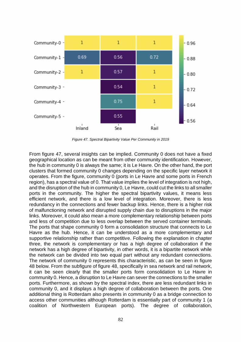
82

Figure 47. Spectral Bipartivity Value Per Community in 2019

From figure 47, several insights can be implied. Community 0 does not have a fixed geographical location as can be meant from other community identification. However, the hub in community 0 is always the same; it is Le Havre. On the other hand, the port clusters that formed community 0 changes depending on the specific layer network it operates. From the figure, community 0 (ports in Le Havre and some ports in French region), has a spectral value of 0. That value implies the level of integration is not high, and the disruption of the hub in community 0, Le Havre, could cut the links to all smaller ports in the community. The higher the spectral bipartivity values, it means less efficient network, and there is a low level of integration. Moreover, there is less redundancy in the connections and fewer backup links. Hence, there is a higher risk of malfunctioning network and disrupted supply chain due to disruptions in the major links. Moreover, it could also mean a more complementary relationship between ports and less of competition due to less overlap between the served container terminals. The ports that shape community 0 form a consolidation structure that connects to Le Havre as the hub. Hence, it can be understood as a more complementary and supportive relationship rather than competitive. Following the explanation in chapter three, the network is complementary or has a high degree of collaboration if the network has a high degree of bipartivity, in other words, it is a bipartite network while the network can be divided into two equal part without any redundant connections. The network of community 0 represents this characteristic, as can be seen in figure 48 below. From the subfigure of figure 48, specifically in sea network and rail network, it can be seen clearly that the smaller ports form consolidation to Le Havre in community 0. Hence, a disruption to Le Havre can sever the connections to the smaller ports. Furthermore, as shown by the spectral index, there are less redundant links in community 0, and it displays a high degree of collaboration between the ports. One additional thing is Rotterdam also presents in community 0 as a bridge connection to access other communities although Rotterdam is essentially part of community 1 (a coalition of Northwestern European ports). The degree of collaboration,

83

competitiveness, and connectivity based on network structure will be explained in great detail in the next chapter since this chapter (chapter 6) focus more on community structure. Furthermore, considering the low spectral bipartivity value across communities in the sea transportation network. The sea transportation network is regarded as the most developed, integrated, and efficient transportation network due to the vast possibilities of route choices and shipping connections. However, the trade-off is in terms of competition between container terminals or communities in sea transportation network due to the redundancy of the links and development of shipping connections develop many overlaps to many served regions between big hubs which create a very competitive environment in this specific network. The detail of this evaluation will be presented in the next chapter about cooperation and connectivity, which leads to the mapping of the sustainability of global hubs. Then, in the aspect of community integration across transportation network, community 1 (a coalition of Dutch ports and Northwestern European ports, including Great Britain) has the highest level of integration and considered the most efficient multimodal transportation community in the overall transportation layers due to the low spectral bipartivity value. The positive aspect and benefit to low spectral value are many connections could be used as a backup if there is a disruption in primary shipping connections. Hence, the network is considered more robust and not prone to disruptions compared to a community or network that has a higher spectral value. However, there are two major hubs in community one, which is Rotterdam and Antwerp. Those hubs have many overlapped in terms of the smaller ports or destinations they serve. Hence, the level of competition is quite high between those two as will be quantified and measured in the next chapter. Furthermore, some additional insights can be concluded in figure 47. Considering community one and two’s presence in all multimodal layer, those communities are considered the most extensive, integrated, and developed communities. Then, community three, four, and five do not have inland spectral value because the inland network does not exist in those communities due to geographical boundary and limitation. There is no natural river that can be used without any significant investment in the development of inland waterways in those communities. Hence, it is more logical and relevant to develop the sea and rail network in those networks. Specifically, in community three (a coalition of Spanish ports) and community four (an alliance of the ports in Great Britain), they can work more to build more railway connections to have more integration and efficient network. Hence, those communities can have more capacity per hour and have a more efficient and resilient network in the end.

84

Figure 48. Network Structure of Community 0 (Le Havre’s Community)

Figure 49 delivers more detailed information about the level of network integration and efficiency of the twelve most versatile hubs across three layers of networks. As indicated earlier, the sea network has the most extensive network since no zero value is shown in figure 49. It means all hubs have a specific community and has interdependence to each other. Moreover, the inland layer has limited by natural boundaries and landscape. Hence, only four hubs that develop a community structure in the network. Most of them are located in the Northwestern region, spreading along Le Havre through Bremerhaven region. Then, the rail network is the second most developed network in the multimodal system. The insight that could be inferred from rail spectral value is there is much room for improvement and development for the hubs or networks in Southern region as indicated from high spectral value that is in line with the earlier analysis of communities’ spectral value in each layer, which means low level of integration and efficiency, and also connect to the hubs that have not connected with the rail community yet, such as Piraeus in Greece, Algeciras in Spain, and Marsaxlokk in Malta. Hence, besides directing the investment for infrastructure development in the sea network, the investment should also see the room of growth in the rail transportation network of Southern European region considering the vast room of progress and improvement in the rail network.

85

Figure 49. Spectral Bipartivity of The Most Versatile Hubs in Each Layer

Figure 50. Spectral Bipartivity of The Most Versatile Hubs per Community

86

The last analysis in this section is the integration or efficiency level of the most versatile hubs in each community in each layer, as shown in figure 50. From the previous analysis, Rotterdam has been identified as the most versatile hubs or the most central container hub in the overall European region due to its connection to many central hubs. However, from figure 50, while Rotterdam connects to most of the communities, it occupies the second position, which is below Antwerp. There is one community connection difference between Rotterdam and Antwerp. Antwerp also connects to the rail community in the Southwestern European region, while Rotterdam has no connection to the rail community in Southwestern European region which is indicated by no spectral value. While the location between Rotterdam and Antwerp is not far away, it has not been investigated what factors drive the development of the connections from community three to Antwerp. The rest of the information is in line with the previous analysis, and Rotterdam is still holding its role as the most central container hub in the overall European region.

6.8. Interlayer Morphology of Community in the European Hinterland Transportation Network

This section will analyze and investigate the morphology of the communities that are formed by the twelve most versatile hubs in Europe. The specific year of choice is 2019 because it is the most recent year, which is considered more relevant to the analysis. Then, the particular network structure is focused on the directed and weighted network connections that represent overall representation of the network in the real practice, which consisting the information about shipping connections and attractiveness of each connection based on shipping frequency. The objective of this section is to study the transition of several container hubs that are part of some communities and observe whether those hubs change the community when in different layers or stay in the same community. As a simplification of information, the information will be presented in forms of aggregated counts of ports in each community and showed the transition of clusters in the shape of the Sankey diagram. As an example, by referring to figure 51, there are two clusters or groups in community rail four (Great Britain container hubs). One cluster stays in the same community, which is community number four, while the other community joins community number one is the sea network. There are three possible drives, which is the flexibility of route choices, more developed infrastructures in the destination community, and greater economies of scale benefit or consolidation, which cause lower transportation cost. Those factors are the factors that make a particular hub more attractive, according to Linde van Wulfften in 2016 (Wulfften, 2016). Specifically, for rail community number five, it should not have existed because there is only one container terminal in rail community number five, which is Istanbul. The consideration is although this network is integrated multimodal network, the cluster should not stand alone in the network, it should be grouped with other ports and form a cluster or community structure together. Hence, by analyzing the connection, rail community number five should be part of community number one in rail network considering the link that formed between Istanbul and Rotterdam.

87

Furthermore, for most of the communities, there are clusters transition to two different layers. More specifically, by breaking down the groups in a particular community, there are movement or shift of the sub-communities that shape a community to two different networks as indicated by bold grey lines in figure 52 as a more explicit example. This type of transition can be observed in community number 0, 1, and 2. It is an indication of the level of multimodal integration. The connection or cluster movement to two different multimodal networks implies the specific communities has a well-developed multimodal infrastructure which connects a different kind of multimodal infrastructure. This observation is in line with the previous observation, and this kind of well-developed multimodal integration can be seen in the Northwestern European region that covers Le Havre to Bremerhaven range. Another observation is the secluded communities or the communities that only exist in a specific network or the communities that its sub-clusters only move to one layer, such as community three, community four, and five. It correlates with low Matthew effect since the clusters in those communities have less preferential connections. Hence, those communities experience or translate to less Matthew effect and also the accumulation of benefits due to the seclusion of those communities. Then, those secluded communities (South European communities) considered have a low integration and efficiency, which is in line with previous investigations in the earlier section as well.

Figure 51. The Morphology of Communities Across Layers in 2019

88

Figure 52. The Transition of the Sub-Clusters to Two Different Transportation Networks

6.9. Chapter Summary and Conclusion This chapter provides a community structure investigated as a continuation of the versatility analysis. This chapter intends to identify community formation in the network. Then, besides community identification, inequality and efficiency aspects of the network have been explained in great detail in this chapter. There are three main findings from the analysis. Firstly, in line with the first law of geography, the container terminals that are near to each other are more likely to be part of the same community and more “intense” connection between them. From the network investigation, it can be seen that if the container terminals are geographically close, the weight of the connection is also relatively higher compared to the container terminals that are separated by a greater distance. On top of the first law of geography, the reason that the container terminals that are close to each other have more frequent shipments is because of the economy of scale. A container terminal prefers to connect to the nearest hub for consolidation to lower the transportation cost. Secondly, the bigger the consolidation hub in a specific community, the more ports will be attracted to the hub, which creates a multiplier effect and attracts more terminals. It creates a more significant inequality effect in the network. However, as presented in section 6.5, the formation of a new community could decrease the inequality gap between communities. Thirdly, the degree of network integration and connectivity can be represented by spectral bipartivity. Spectral bipartivity is often be called as a measure of the degree of efficiency in the network. The findings from this study are the sea network has the highest degree of network efficiency compared to the inland and the rail network. Hence, the sea network has a higher degree of connectivity and a more significant number of route choices.

89

From those findings, several recommendations can be suggested. First, the inter-community connection can decrease the inequality in the network and increase the degree of connectivity between communities. It will be beneficial to have a more significant route choice between communities. Then, the connection between different community can improve the redundancy and lower down the spectral bipartivity index. By having a higher redundancy, it means more significant backup connections in case of failures in the backbone connections. However, a greater redundancy will come at the cost of more overlaps of hinterland destinations between hubs, which creates a competitive environment between hubs and decreases the collaboration between hubs. The next chapter, chapter 7, will provide greater detail about cooperation and connectivity.

90

Chapter 7: The Relationship Structure Between European’s Versatile Ports

7.1. Introduction In the previous chapter, community investigation has been performed on the network. Then, various measurements of the specific communities have been performed, such as the community discoveries, inequality or Matthew Effect observation in each community, level of efficiency, interdependence, and morphology of each community have been analyzed. This section intends to complement the analysis and set the foundation for the discussion section about criticality of the network. The objective of this section is to provide supporting information regarding cooperation and connectivity of the hubs. Then, by utilizing cooperation and connectivity aspect of the hubs, mapping and classification of the hubs into sustainable or unsustainable, regional or global hub status can be defined and determined. Afterwards, based on the information in this chapter, criticality analysis can be performed and discussed in the following chapter.

7.2. Quantification of Cooperation and Connectivity Index in the EHTN As explained in chapter three, the analysis is based on the NHPA model by investigating the cooperation and connectivity of the hubs based on its network structure (Low et al., 2009). As stated earlier, NHPA has two main components, which is the quantification of connectivity and cooperation. Connectivity measurement is crucial to determine the status of the hubs and classify, whether it is regional or global hubs based on its connectivity index. The degree of connectivity is an indicator of overall accessibility and coverage of the hubs itself. Then, the cooperation index is a measure that determines the sustainability status of the hubs. The hubs that have minimal overlaps in terms of served destinations will have a more complementary relationship and less competition. Therefore, it creates a win-win solution between hubs (Low et al., 2009). This situation may create a stronger regional strength due to the complementary and collaboration effect in the network. High cooperation index depicts a more sustainable characteristic of the hub. On the other hand, the low cooperation index may portray a vulnerability of a specific hub because of its vulnerability to the loss of the traffics due to the shift of the shipping schedule of major carriers (Low et al., 2009). This chapter will present the pairwise cooperation between hubs in each layer, such as the sea network, the inland network, and the rail network. Then, it will be followed by overall cooperation and connectivity measurement in the aggregate network. Afterwards, the hubs will be classified into regional or global and sustainable or unsustainable hubs. This chapter will also prove or validate some of the behaviours in the community analysis part, such as the drop in Rotterdam’s connection strength due to the appearance of the new community. The question such as “how is the relevance to the drop in the new community to the drop of connections in leading main hubs?” can be answered and validated in this chapter. This section will present four folds of information, such as a pairwise comparison between hubs, aggregate cooperation index, connectivity index, and the relevance of

91

community identification to the collaboration between hubs. The information will be assessed in each individual network and analyzed whether the tendency happened in all layers of the network. There are four graphs that will be presented in this section to help the explanation and insights that were gained from the analysis. Four graphs will present the network measurements in each layer of the multimodal transportation network. In a single graph, there are four different information that is presented. Firstly, on the most left and bottom of information, some numbers are positioned in line with the naming of each hub. Those numbers are the identification of the communities that are the results from the analysis of the previous chapter. Then, there are three heatmaps in the middle of the graphs, those are pairwise cooperation index between hubs, aggregate cooperation index, and connectivity index in sequence from top to bottom. The pairwise cooperation index quantifies and presented the cooperation between two hubs. As explained in chapter 4, the cooperation between hubs are based on overlaps in the hinterland destinations, the more overlaps then the more competitive the relationship of the hubs. Then, it is considered the hubs are more vulnerable to the loss of traffics due to the shift of the major carriers’ services and shipping schedules (Low et al., 2009). Then, the aggregate cooperation index is the sum of cooperation index in a particular hub based on its cooperative relationship with other eleven hubs that are spread through the European continental region. Aggregate cooperation index might not be a perfect measurement because it only considers the twelve most versatile hubs that are scattered on the general European region. However, it is a very useful measurement to gain a holistic representation of the current competitive landscape in Europe. By adding more hubs, it might provide a more accurate representation of the landscape. However, those twelve hubs have depicted all existing communities through European continents. Therefore, the representation will be near accurate, although not perfect. The last one is the connectivity index, it is the modification of the Hansen integral that measures the accessibility of the network (Low et al., 2009; Taylor, Sekhar, & D’Este, 2006). The connectivity index is a more comprehensive measurement than aggregate cooperation index because it considers all links and nodes in the network (Low et al., 2009). Please refer to chapter 3 and 4 for the technical and mathematical details. The expected outcome is when the hubs are in the same community, it is expected to have a high degree of competition or low cooperation index. This is due to the expectation that if the hubs exist in the same community, then there will be many overlaps in the hinterland destinations between them. Hence, the hubs will compete to serve the same hinterland destinations and create a competitive atmosphere by offering a superior service compared to the others rather than focusing on building collaboration with other hubs, and enhancing the strength of coalition and develop partnerships with other hubs which will enhance the regional economic welfare. The following results will use colour-coding to focus on a particular tendency of the relationship. The colour index will span from a very dark blue to yellow. The dark blue colour will mark lower value and yellow will mark high measurement value. The lighter the colour, the higher the value is. From the graph of the sea network, which is figure 53. Antwerp has the lowest aggregate cooperation index, and Bremerhaven has the highest aggregate

92

cooperation index. Then, in terms of connectivity, Rotterdam is the most well-connected hub and Southampton is the least well-connected hub. By looking at the pairwise cooperation index, Rotterdam and Antwerp have a cooperation index of 0.15 which is very low. This is because Rotterdam and Antwerp are relatively close to each other and stays in the same community which is community one. Therefore, hinterland destinations overlaps are expected between both of them which is the reasoning of high competition between Rotterdam and Antwerp. However, while the presence of the hubs in the same community will increase the expectation of hinterland destinations overlaps and high competition landscape, it does not necessarily have that particular situation. For example, Antwerp’s relationship with Felixstowe in the UK and Le Havre produces a low pairwise competition index, which is 0.099 and 0.11 respectively, both of Felixstowe and Le Havre have a different community to Antwerp. Hence, the overlap of hinterland destinations is the main point here. However, both Felixstowe and Le Havre are still considered relatively close to Antwerp, which is part of the Northwestern European region, although they exist in different communities. Furthermore, Bremerhaven demonstrates the same behaviour as the previous example. Bremerhaven has the highest aggregate cooperation index in the sea network with mediocre connectivity index. Bremerhaven gains a very high pairwise cooperation index with Algeciras, Barcelona, and Le Havre. Those three hubs are located in different communities to Bremerhaven. Then, in terms of geographical location, it is relatively far separated from each other. Therefore, there is a minimum number of hinterland destination overlaps between them. Moreover, Bremerhaven has a very low pairwise cooperation index with Hamburg. This is also due to the hinterland destination overlaps and both of them serves German region which is a conflict of interest and high competition relationship between them. The rest of the hubs in the sea network depicts the same relationship. Then, the rest of the network, which is inland, rail, and aggregate network, also demonstrates similar behaviour as can be observed in figure 54, 55, and 56. Competition may benefit the customers that lower down the logistical cost. However, it can be argued that too much competition will create a win-lose situation and drop the regional economic welfare.

93

Figure 53. Pairwise Cooperation Index, Aggregate Cooperation Index, and Connectivity Index in The Sea Network

Figure 54. Pairwise Cooperation Index, Aggregate Cooperation Index, and Connectivity Index in The Sea Network

94

Figure 55. Pairwise Cooperation Index, Aggregate Cooperation Index, and Connectivity Index in The Rail

Network

95

Figure 56. Pairwise Cooperation Index, Aggregate Cooperation Index, and Connectivity Index in The Aggregate

Network

7.3. Correlation between Cooperation and Connectivity The additional information that closes this section is to observe the correlation between aggregate cooperation behaviour and connectivity. The expected behaviour that is interesting to be explored is whether the higher the connectivity index, will it also increase the possibility of hinterland destination overlaps? In other words, the higher the connectivity is, the lower the cooperation between ports? What is the correlation index in each multimodal transportation network? The correlation index in rail, sea, inland. Inland and rail exhibit previous tendency but with stronger index. Hence, higher correlation leads to a high possibility of cooperation-connectivity overlap. The correlation for the sea network, inland network, and rail network are -0.38, -0.99, and -0.86 respectively. The inland and rail network has the highest correlation index. From the exhibit, please refer to figure 57 to see the scatter diagram, it could be understood that the higher the correlation index is, then it will present a stronger tendency of the previous behaviour. The rail network demonstrates the higher cooperation value between hubs that have different communities and lower

96

connectivity, unlike the sea network. For example, in the sea network, Antwerp and Felixstowe have a low pairwise cooperation index, this is due to the relatively close location between each Antwerp and Felixstowe, and also the overlaps between them. In the rail network, the relation is more straightforward. If the hubs have different communities, then it demonstrates a high pairwise cooperation index which is not necessarily the case in the sea network. In the rail network, the tendency is the more connected the hubs are, then the lower is the aggregate cooperation index. It also implies that in the rail network, the more connected the hubs are, then the more overlaps are likely to happen between hubs, which lower is aggregate cooperation index. Moreover, the inland network also exhibits a similar tendency, but the sample is relatively small compared to the rail and the sea network. Then, Le Havre has different communities to all eleven hubs. But, from its geographical location, it can be learned that Le Havre is a part of Northwestern communities and it has a lower aggregate cooperation index with more overlaps to Northern rail transportation hubs. From the previous example, it can be concluded that the higher the correlation index in the network, then it exhibits the stronger inverse relationship between connectivity and cooperation. In other words, it is more likely to have overlaps between hubs in the same communities or the hubs are geographically close to each other when a particular network has a higher correlation index. More explanation about the relationship between network structure, the redundancy is network structure, and spectral value will be explained in the next chapter, the discussion chapter and robustness analysis. This section will continue with the classification of the sustainability of the hubs.

7.4. Sustainability of the Hubs From the analysis of the earlier section, the connectivity and the aggregate cooperation index have been determined. The next step is to plot it into a cartesian coordinate. The objective of this step is to investigate and classify the sustainability and hub status of the most versatile ports. The aggregate cooperation index will define the sustainability status of the hubs. It means higher collaboration will lead to a lower risk of traffic loss if major services streamline their shipping schedules (Low et al., 2009). Furthermore, the connectivity will define the hubs into regional or global hubs. The reasoning is the more critical the status of the hub or the higher the role of the ports in the global transhipment chain, then the container hubs should have higher accessibility and more well-connected to the global chain. The connectivity index is based on the modification of Hansen integral that indicates the accessibility of the container hubs. Based on that index, it can be grouped into a regional or global hub. In this context, the point of comparison is to other eleven hubs and the classification to regional or global hub status is based on the relative comparison with other eleven hubs. The reason is because of the lack of data or information on other container hubs in other parts of the globe. This limitation can be tackled by adding new information. The author does not have access to that information currently. However, by utilizing the existing information, it can provide some insights about the relative positioning of the European ports relative to each other, which is the focus and scope of this study.

97

The classification of the hubs can be seen in figure 57. There is four visualization that is provided in this study, which is the sea network, inland network, rail network, and aggregate network. While the explanation of the sea, inland, and rail network are very straightforward, the aggregate network is the unification of those networks. In the aggregate network, all of the nodes, which is the container hubs, are combined together in one layer of the network without considering its modality. In this point, only the location of the nodes, the connections, and its overlapped hinterland destinations that are considered. Then, the aggregate cooperation index and the connectivity index were calculated by using the same method as each independent network. The aggregate network will be useful to provide us with the more comprehensive and helicopter or more general view of the hub status and sustainability of the container hubs. From figure 57, both of the most versatile hubs in Europe, which is Rotterdam and Antwerp were classified as unsustainable hubs. As explained before, this is because of the overlaps in the hinterland destinations of those ports. Most of the overlaps also happened between Rotterdam and Antwerp. Hence, both of those hubs have a very competitive relationship with each other. Rotterdam also has overlaps to other regions besides Antwerp. Therefore, it can be concluded that high connectivity and accessibility could come at the cost of collaborations or partnerships. However, it depends on the network it operates in as explained in the previous section. In this case, the consideration is the network structure, such as the redundancy of the network which can be quantified by using spectral bipartivity, which leads to the shape of the network. The more redundant the connections in the network, then the network tends to have a distributed structure rather than pure scale-free structure although preferential attachment will still happen in both cases. The detail of this discussion will be elaborated in the next chapter. The main point is the more redundant connections exist in the network (lower spectral bipartivity index) and the more the network imitates a distributed structure, then the correlation between connectivity and aggregate cooperation index will be more prevalent, which happens in the rail and the inland network in this study. To sum up, the main objective of this section is to map the sustainability of the most versatile hubs and how the hubs are relatively positioned to each other. The target of every hub will be to achieve global and sustainable status in this context. The higher or the more global the hub status is, then the hub will have higher influence and more integral role in the global supply chain. Then, if the hub is considered sustainable, there is little risk that threatens the role of the hub in the logistic chain. From the aggregate network standpoint, the hub that achieves that status is Hamburg due to its collaboration and complementary relationship with other ports. The contributor to its high cooperation index is Hamburg’s relationship with other hubs in the sea network. Hamburg has a high collaboration with many ports and keeps hinterland destination overlaps at a minimum in the sea network. Hence, Hamburg is considered sustainable and the existing relationship will not backfire to its position in the network, considering the risk of the changes in the traffic of the major services. Moreover, Rotterdam and Antwerp should develop a more healthy relationship and establish more cooperative and partnerships with other hubs in the network. The correlation of aggregate network is -0.31. Then, the higher the connectivity does not mean of many hinterland destination overlaps. It is to replicate a distributed

98

network structure with many direct independent connections and little chance of overlaps. However, from the tendency, to connect to further regional will still be expected to strengthen the partnerships.

Figure 57. Sustainability and Hub Status Matrix of The European Hubs

7.5. Chapter Summary and Conclusion This chapter intends to provide more detailed information on the cooperation and connectivity relationship between hubs. Then, based on that information, the sustainability of the hubs can be mapped. This point of view of sustainability is based on the degree of threat from the potential shift of the shipping schedules by major shippers. Figure 57 presents the findings of this study and classified it based on four different networks. Based on this, the recommendation is to minimize the number of hinterland destination overlaps to achieve a high degree of cooperation while maintaining a high degree of connectivity. Based on the map, the target quadrant in the top right of the matrix. The next chapter will discuss the results from three sections, provide additional analysis about market structure and competition, customers benefit, analyze the relationship between network structure, redundancy in the connections (spectral index), correlation index of cooperation-connectivity, and Matthew effect (inequality) of the hubs. Then, robustness analysis will be performed as a verification/validation method. Last but not least, all of the research questions will be answered, which is the main goals of the study.

99

Chapter 8: Discussion

8.1. Introduction The objective for this chapter is as a chapter which integrates all of the analysis that has been performed previously. There are three discussions in this chapter, which is criticality, vulnerability, and efficiency of the European Hinterland Transportation Network. The discussion about criticality will emphasize the criticality and importance of the most central or versatile node to the overall network. The discussion of the efficiency of the EHTN will focus on the redundancy of the EHTN. Redundancy, in this case, can be thought in the context of backup connections or backup nodes in there are some disruptions to the origin or destination points. Then, the chapter will be concluded by answering the research questions that have been defined at the beginning of this report.

8.2. The criticality of the European Hinterland Transportation Network In this section, the criticality assessment will be performed. There are three variables to measure the impact on the network. Firstly, the network diameter will be used as an indicator for coverage and reach of the network. The network diameter is a variable that measures the degree of the longest path length from the list of possible connections in the network. Secondly, the mean path length is an indicator of the average shortest path for all possible connections in the network. The shortest path can be used as an indicator for the level of integration in the network and also the coverage of the network like network diameter (Beygelzimer, Grinstein, Linsker, & Rish, 2005; Mandke et al., 2018). The lower the mean path length, then there are more route options or the density of the network (edges per nodes) are higher. Hence, the network is more integrated, and since there are more route choices, there are more possible connections from one origin to a particular destination, therefore, the mean path length will be lowered. However, in the case of disruptions, the mean path length can also be lowered down due to the less coverage of the network. The targeted disruptions of community leaders will disconnect important hubs and disable important connections which make the network smaller. Therefore, the mean path length will appear smaller as a result. Thirdly, the network density or edges per layer is a measurement of route choices in the network. The change in those three network diagnostics variables will be used to measure the transformation in the network from three-point of views in the case of disruptions in the leader of each community. Diameter is an indicator of coverage, mean path length is an indicator of network integration, and density is an indicator of the degree of route choices. Then, the usage of those three indicators together can be used as a “criticality” indicator. By doing targeted disruptions to each community leader, the change in those three indicators can describe how critical is the community leaders to the overall network performance (in terms of coverage, integration, and degree of connections). In other words, it can be understood how community leaders can influence the overall network performance.

100

Table 4 presents the twelve most versatile container hubs in Europe with its community identification number as identified in chapter 5 and 6. Moreover, the hubs were presented in sequence starting from the most versatile or the most central hubs to the least central hubs. Then, based on this information, the leader or the most central hub from each community are presented by table 5. Since five communities have been identified earlier, there are five leaders in table 5, each leader is a representative of each community. The next step is to perform a targeted disruption to the leaders of each community, then measure the change in the overall network performance to know how sensitive the network performance per layer will be affected in the case of targeted disruption.

No Ports Community

1 Rotterdam 1

2 Antwerp 1

3 Hamburg 2

4 Bremerhaven 2

5 Valencia 3

6 Piraeus 5

7 Algeciras 3

8 Felixstowe 4

9 Barcelona 3

10 Marsaxlokk 5

11 Le Havre 0

12 Southampton 4 Table 4. Ports and Community Identification

Community Leaders

1 Rotterdam

2 Hamburg

3 Valencia

4 Felixstowe

5 Marsaxlokk Table 5. Community Leaders

The results in the network diameter before and after disruption will be explained per network layer, such as sea layer, inland layer, and rail layer due to the different structure between each layer. Sea layer has more redundancy in the connections of the network (as indicated by spectral bipartivity index as explained in chapter 6) which make the role of the hubs less centralized (or less scale-free) compared to inland and rail network. The sea network is more inclined to the distributed structure. However, since the network still follows a hub-and-spoke structure, the consolidation structure is still present in the network. The inland and rail network follows a more centralized network structure, as indicated in chapter 3 and has more inclination to a hub-and-spoke structure. This is because of the role of the hub as a consolidation point that aggregates the shipments from several origins to push the efficiency of transportation, which will lower the transportation cost in the end. The implication of this structure to

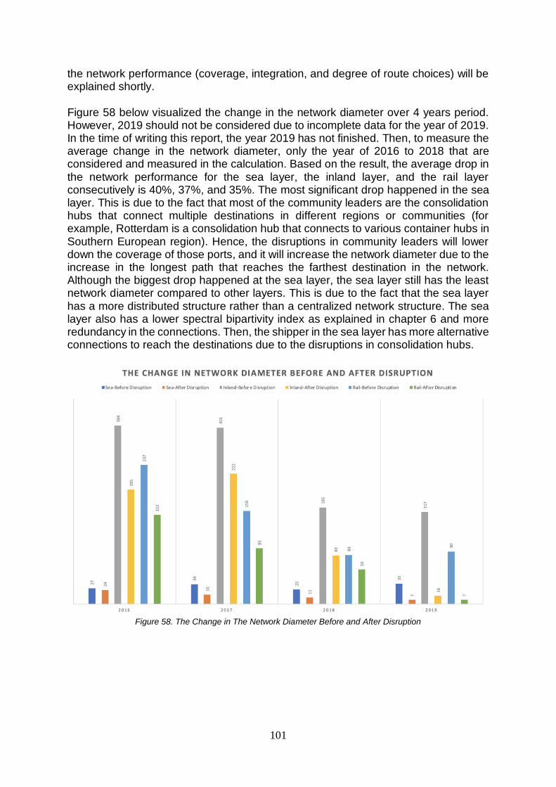
101

the network performance (coverage, integration, and degree of route choices) will be explained shortly. Figure 58 below visualized the change in the network diameter over 4 years period. However, 2019 should not be considered due to incomplete data for the year of 2019. In the time of writing this report, the year 2019 has not finished. Then, to measure the average change in the network diameter, only the year of 2016 to 2018 that are considered and measured in the calculation. Based on the result, the average drop in the network performance for the sea layer, the inland layer, and the rail layer consecutively is 40%, 37%, and 35%. The most significant drop happened in the sea layer. This is due to the fact that most of the community leaders are the consolidation hubs that connect multiple destinations in different regions or communities (for example, Rotterdam is a consolidation hub that connects to various container hubs in Southern European region). Hence, the disruptions in community leaders will lower down the coverage of those ports, and it will increase the network diameter due to the increase in the longest path that reaches the farthest destination in the network. Although the biggest drop happened at the sea layer, the sea layer still has the least network diameter compared to other layers. This is due to the fact that the sea layer has a more distributed structure rather than a centralized network structure. The sea layer also has a lower spectral bipartivity index as explained in chapter 6 and more redundancy in the connections. Then, the shipper in the sea layer has more alternative connections to reach the destinations due to the disruptions in consolidation hubs.

Figure 58. The Change in The Network Diameter Before and After Disruption

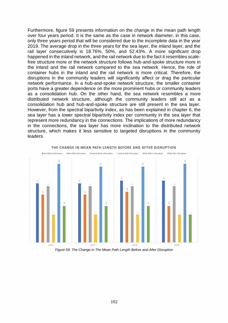
102

Furthermore, figure 59 presents information on the change in the mean path length over four years period. It is the same as the case in network diameter, in this case, only three years period that will be considered due to the incomplete data in the year 2019. The average drop in the three years for the sea layer, the inland layer, and the rail layer consecutively is 18.76%, 50%, and 52.43%. A more significant drop happened in the inland network, and the rail network due to the fact it resembles scale-free structure more or the network structure follows hub-and-spoke structure more in the inland and the rail network compared to the sea network. Hence, the role of container hubs in the inland and the rail network is more critical. Therefore, the disruptions in the community leaders will significantly affect or drag the particular network performance. In a hub-and-spoke network structure, the smaller container ports have a greater dependence on the more prominent hubs or community leaders as a consolidation hub. On the other hand, the sea network resembles a more distributed network structure, although the community leaders still act as a consolidation hub and hub-and-spoke structure are still present in the sea layer. However, from the spectral bipartivity index, as has been explained in chapter 6, the sea layer has a lower spectral bipartivity index per community in the sea layer that represent more redundancy in the connections. The implications of more redundancy in the connections, the sea layer has more inclination to the distributed network structure, which makes it less sensitive to targeted disruptions in the community leaders.

Figure 59. The Change in The Mean Path Length Before and After Disruption

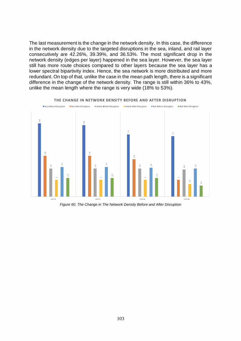
103

The last measurement is the change in the network density. In this case, the difference in the network density due to the targeted disruptions in the sea, inland, and rail layer consecutively are 42.26%, 39.39%, and 36.53%. The most significant drop in the network density (edges per layer) happened in the sea layer. However, the sea layer still has more route choices compared to other layers because the sea layer has a lower spectral bipartivity index. Hence, the sea network is more distributed and more redundant. On top of that, unlike the case in the mean path length, there is a significant difference in the change of the network density. The range is still within 36% to 43%, unlike the mean length where the range is very wide (18% to 53%).

Figure 60. The Change in The Network Density Before and After Disruption

104

8.3. Special Case of the Disruptions in The Port of Rotterdam As the biggest container hub and the most central container hub in the network, the criticality of Rotterdam is essential to be assessed to see its impact on each layer. In this case, only two network performance that will be presented, which is the network diameter and the network density because there is relatively little change in the mean path length, and it is less insightful to show the result in the mean path length. The change in the network diameter for three years period (from 2016 to 2018) are -14.43%, -0.5%, 27.82% for the sea, inland, and rail layer. As explained earlier, the change in the network diameter means the difference in the coverage of the network. Coverage, in this case, is the longest path available from all available connections in the network. For the disruption in Rotterdam, there is a drop of 14.43% in sea layer because Rotterdam is the central hub that connects container hubs in different communities. Due to the disruption in Rotterdam, the smaller ports in a different or farther location are disconnected, and the network has less coverage because of it. The inland layer has less change due to there are several big hubs that could act as a backup or substitute hub due to the disruption in Rotterdam, such as Antwerp, Hamburg, and Bremerhaven. However, the compelling case is for the rail network, the network diameter is increasing in the rail network. This does not mean more coverage since it is illogical to assume so due to the disruption. Instead, because the rail network is more inclined to hub-and-spoke structure and follows a centralized network structure more (where the case of preferential attachment happens here), the disruption in a critical hub, like Rotterdam, will add more difficulties and break down important link that connect an origin and a far-located destination that previously connected by the hub. The disruption in the consolidation hub will cause a farther workaround and make the path longer, which connects an origin and far-located destination. Therefore, there will be an increase in the network diameter in this case.

Figure 61. The Change in The Network Diameter for The Disruption in Rotterdam

105

The change in the network density due to disruption in Rotterdam is -6.46%, -59.59%, and -10,56% for the sea, inland, and rail layer sequentially. The most significant drop happens at the inland layer because the inland network is focused on the Northwestern European region with the Rotterdam as the most critical consolidation hub there which links all important hubs, origins, and destinations. Hence, the disruption in Rotterdam will have a significant impact on the network density of the inland layer. Therefore, due to the disruption, the inland layer will have the least route choices (edges per layer) compared to other layers. Before the disruption, the network density of the inland layer and the rail layer is close although the inland layer still has the least density of all.

Figure 62. The Change in The Network Density for The Disruption in Rotterdam

8.4. The efficiency of the European Hinterland Transportation Network In the event of a disruption, it is essential to understand the availability of backup connections or redundancy of the connections in the network. The redundancy of the connections in the network is also called as “efficiency” of the network (Estrada & Gómez-gardeñes, 2016). Then, the degree of network efficiency can be implied by the degree of spectral bipartivity. The spectral bipartivity index from 2016 to 2019 is presented by figure 63. As mentioned earlier, the spectral bipartivity index for the year of 2019 may still change because, at the time of doing this project and writing the report, it is still in the middle of the year 2019. From 2016 to 2019, the mean of the spectral bipartivity index can be put in sequence (from lower to higher) starting from the sea layer, the rail layer, and the inland layer. The sea layer has a low spectral bipartivity index compared to the

106

other two layers. While the degree of spectral bipartivity in the inland and the rail network are relatively close. From the degree of spectral bipartivity in four years range, we can conclude that the sea layer has a more distributed structure with more redundancy in the connections. Hence, the disruption in the community leaders or an important consolidation hub in the sea layer has less impact to the overall mean path length in the network based on possible links that connect a pair of origin and destination. This situation is caused by the availability of backup connections and links in the network. In the sea layer, the shippers can utilize a different path or easily find a workaround in the case of the original path is severed due to unexpected disruption. On the other hand, in the inland and rail network, there is less chance to establish a new connection or find a different path as a replacement for the disrupted path due to the centralized structure of the network. In other words, once the original connection is severed, then the connection is lost and cause a significant impact on the network (in terms of mean path length or established connection). Moreover, it will further inhibit the goods movement due to the severed connection due to the unavailability of backup links. To conclude this section, the sea layer is a more efficient network compared to the other two layers (the inland and the rail layer) as represented by its lower spectral bipartivity index. Then, it can also be inferred that the sea layer with its more distributed network structure is more resistant to targeted disruptions to its consolidation hubs.

Figure 63. The Spectral Bipartivity Index from 2016 to 2019

107

8.5. Chapter Summary and Conclusion This chapter discusses the criticality in EHTN and also the efficiency of the EHTN. The criticality of EHTN shows the role of community leaders is more critical in a more centralized (hub-and-spoke) network structure as shown in the earlier analysis. Hence, the centralized network structure, which is based on preferred attachment for the relationship between container hubs, is more sensitive to targeted disruptions or disruptions to its community leaders. The more distributed the structure of the network is, as shown by the degree of spectral bipartivity, the less sensitive the network to disruptions to its community leaders. Therefore, the role of community leaders is less critical in a more distributed network structure (does not necessarily not important since the role of the hub is still significant to make the network well-functioned). Then, to make the network less sensitive to targeted disruptions, more redundancy in the connections can be improved that will push the degree of spectral bipartivity lower. Practically, more redundancy in the connection will make the network has more route choices and increase the network density (edges per node), which improve the number of alternative connections in the event of disruptions or malfunctioning hub or edges. However, the improvement of redundancy in the connections will increase the number of overlapped destinations between hubs which increase the degree of competition between hubs. While on the one side, it will benefit the customers which will lower down the logistics cost due to the improvement in competition. On the other side, it will put more strain or pressure on the container hubs to keep the competitiveness and increase the degree of competition. If the degree of overlap is too much (which is not the scope of this study to determine it), then it will be unsustainable for the ports because of the possibility that leads to unhealthy competition.

108

Chapter 9: Conclusion and Future Research

9.1. Introduction The objective of this chapter to reflect back on the results and revisit each research question. Moreover, the main goal of this chapter to answer the main research question which is related to the knowledge gaps that were identified earlier. Then, this chapter will conclude the results of the study. This chapter will begin by revisiting and answering each research sub-question. Then, by answering each research sub-question, it will continue to answer the main research question which the goal of the study is. Then, this chapter will be closed with a recommendation section which is the end result of this study and links it to the development of the transportation network structure along four years results. To answer the main research questions, five research sub-questions have been defined. The answer to each research sub-question will be presented in the next section. Then, section 9.4 will combine all of those answers and provide an answer to the main research question.

9.2. Answering Research Sub-Questions

1. How can the versatility of European Hinterland Transportation Network be measured by utilizing network theory?

There are two types of methods to analyze the network structure. Firstly, the network components (nodes and edges) can be placed in a single aggregated network layer. Then, the analyze can be performed in that single network layer. Secondly, it is also possible to treat and divide the network components into multiple distinct layers. The second method is called a multilayer network analysis. The disadvantage of the first method to rank the most central or versatile container hubs is it may have missing information if some nodes have the same degree of connections. Let’s suppose some nodes have the same degree of connections while the nodes are located in different layers. By aggregating those nodes in a single aggregated network, the information and distinction between layers will be missing. As a result, in a single aggregated network, those nodes which have the same degree of connections will have the same rank while it should not be the case. That issue can be overcome by treating and separating the network components into different layers, which is each network component of innate characteristics. Therefore, there is no missing information and the result of the analysis will be more detailed due to its layer separation compared to a single aggregate network. Moreover, the end result of the versatility rank will be more distinctive and the number of “same” rank (which is related to network aggregation problem) can be minimized. It was stated minimized because there is still a possibility that the same rank could happen due to the same degree of the nodes in the same layer. However, by adding more information, such as assigning a weight to the connections between nodes, this problem can be further minimized, and the end result will be more specific.

109

2. How can collaboration and competition among European container hubs be

evaluated based on its network topology? Different communities are shaped by the shipping schedule and frequency. In other words, the intensity of the connections or degree of connectivity between origins and destinations forms several distinct community clusters. In this case, the strength or the intensity of the connections between container terminals in the same identifiable communities are stronger compared to the links between different clusters. Therefore, the clusters can be identified by utilizing multilayer infomap algorithm based on this logic. Every cluster has some container hubs that act as the leaders in the specific clusters. Then, if there are some influential nodes that are located in the same community, it opens the possibility of a competitive relationship. This relationship is related to the idea that is first introduced by Waldo Tobler in 1970: “Everything is related to everything else, but near things are more related than distant things” (Tobler, 1970). This study explored the first law of geography in the European multimodal transportation context. Once cluster identification has been performed and the network components (container terminals) have been identified as a part of a particular cluster. Then, the first law of geography came into action and the relationship between terminals that are linked to this law can be explored. A question like “will the container hubs in the same community (that have a relatively closer relationship compared to the relationship between hubs in different communities) have a higher degree of competition?” and “what kind of network structure that causes a high degree of competition between container hubs in the same community?” As an example, Rotterdam and Antwerp are the biggest container hubs in the community one and based on the result of quantitative analysis that was performed in this study, Rotterdam and Antwerp have a low collaboration index (very high competition between Rotterdam and Antwerp). To explore this relationship quantitatively and by using complex network science method, two network structures will be defined as the main building blocks to perform the analysis. According to NHPA (network-based hub port assessment) model, the port cooperation index can be quantified by referring to two network structures, which is perfect complementary relationship and perfect competitive relationship (Low et al., 2009). An ideal complementary relationship is a relationship between two hubs without any overlapped in the destinations that are served by those hubs. On the other hand, an ideal competitive relationship is depicted when all of the served destinations are completely overlapped between two hubs. Then, for the latter, the hubs will compete with each other to protect its market share and its income in the end. Another reason is in a highly competitive environment, the lost in the competition will affect a particular hub negatively and threaten the sustainability of the hubs itself. To sum up, the degree of competition or collaboration between hubs can be assessed by utilizing the NHPA model and by measuring the degree of destinations overlaps between two hubs. Additionally, based on the first law of geography, the hubs in the

110

same community are more likely to have a high degree of competition between them due to an inherent closer relationship between them. The detail of the analysis was explained in great detail in chapter six and seven.

3. How to map the sustainability landscape of European biggest container hubs based on its network structure?

From a network standpoint, the connectivity index indicates the degree of accessibility of the container hubs (Low et al., 2009). The connectivity index provides a hint of the inclination of the hubs to become a global hub (Low et al., 2009). Then, by combining connectivity index with cooperation index which measures the degree of collaboration between ports, the sustainability of the network connectivity between a hub with other container terminals can be assessed (Low et al., 2009). Please take notice that this is not a single measure to determine the sustainability of the ports due to the sustainability of the ports will depend on many variables that are not in the context of this study, such as sustainability of the power sources and geopolitical relationship between countries. The sustainability that becomes a focus of this study if the sustainability of the connectivity based on network structure and connectivity point of view which follows the NHPA framework. For the hubs that have minimal overlaps to other hubs, it ensures the complementary and high degree of collaboration between them. Hence, the relationship creates a win-win condition. The high degree of cooperation will ensure the positioning of the ports in the network (Low et al., 2009). If the hubs have a high degree of competition, then the hubs are prone to engage in an intense rivalry relationship. This kind of relationship is due to the vulnerability due to the shift of major carriers if a hub is less attractive compared to other hubs. Then, based on the earlier explanation, if the minimum overlap in the hinterland destinations will benefit and secure the positioning of the hubs, why the market structure moved towards the competitive environment and the government concerns to reduce the trade limitation between countries if it does not strengthen the position of the ports? In this case, a point of view from shippers need to be used to understand the trade-off. A more hierarchical network structure which follows the scale-free structure and preferred attachment structure (hub-and-spoke), which ensure minimum overlap in hinterland destinations, will create a possibility of cartel or domination of bigger hubs to smaller hubs. On the other hand, more “flat” or distributed market structure, as in the case of sea network, will create a more competitive environment which will lower down the logistical cost due to the competition. The “flatness” of the structure can be measured by utilizing spectral bipartivity index that has been conducted in this study. The lower the spectral index, then the more “distributed” the network structure. While the more distributed and competitive structure will benefit the consumers (in terms of cost), the trade-off is in terms of the vulnerability to the shift of major carriers shipping schedules which puts a strain on the position of the hubs (Low et al., 2009). On the other hand, the highly hierarchical structure based on preferred attachment, which is the common structure in European multimodal transportation structure as

111

investigated in this study (inland and rail network), will create a Matthew effect (the rich get richer, and the poor get poorer) and inequality in the network (underdeveloped Southern communities). The trade-off of a more hierarchical structure is while it benefits or strengthens the positioning of the hubs based on complementary relationship, it will have the possibility to have a “cartel-like” relationship and oligopoly that will create the Matthew effect exist in the network. Therefore, it will drive up the logistical cost. Furthermore, the structure based on the preferred attachment will create a node is more influential than the others and increases the dependence of the rest of the networks to several community leaders. As a result, this structure will be more prone to targeted disruption (the inland and rail network) rather than “distributed” network structure (as the case in the sea network). Therefore, to overcome this kind of issue and push the development in Southern Europe, the European Commission introduced the TEN-T project to promote the development of nine corridors throughout Europe. As a result of this study, it creates a more “equal” network structure and more distributed development in the entire European region. Moreover, it makes the network less sensitive to targeted disruption, as will be discussed in the next research question. To conclude this section, sustainability can be classified into two types of sustainability. Firstly, the sustainability that is based on the vulnerability or threat to the shift of significant carriers’ shipping schedules. A highly competitive environment with many destinations overlaps, and a low degree of cooperation is prone to the shift of the carriers. Hence, it is categorized as an unstable and unsustainable relationship due to the threat from the carriers. Secondly, the sustainability that is based on the targeted disruption, the more “hierarchical” the network structure is, the more vulnerable and sensitive the network to targeted disruptions that affect the whole network. To map the sustainability of the first category, the container hubs can be plotted based on its degree of connectivity and cooperation. As explained earlier, the degree of connectivity will determine the “regional” or “global” hub status, while the cooperation will determine the sustainability of the relationship. Regarding assessing the sustainability of the second category, it will be answered in the next research sub-question, which is related to network performance.

112

4. How will a network’s performance be affected by removing some particular central or versatile nodes (hubs)?

The network’s performance can be measured in three ways as presented in chapter 8, such as by network diameter, by the mean path length, and by the network density. Firstly, the network diameter was used to measure the coverage of the network. It is the representation of the coverage because network diameter is the shortest path that measures two farthest nodes. The degree of network diameter can be decreased in the case of less coverage or the most distant node disconnected due to the change in the connections or the disruption of the hub as performed in the study. Moreover, the network diameter will improve in the case of an additional node that replaces the furthest node or the disruption of the hub in a scale-free network structure which will enhance the difficulties to reach the most distant nodes. Therefore, the network diameter will grow in that case. Secondly, the mean path length measures the level of integration of the network (Beygelzimer et al., 2005; Mandke et al., 2018). Moreover, the mean path length can also represent coverage like the network diameter. The lower the mean path length, then it means the “agent” or shippers in multimodal context only need less step to go from one origin to a destination. Hence, the lower the mean path length, it means the network is more integrated because there are more route choices which make travelling inside the network easier due to a greater number of connections to choose from. Therefore, it will lower down the overall mean path length. However, in the case of targeted disruptions as presented in chapter 8, the mean path length can be lowered down due to the less coverage of the network. The disruptions of community leaders in the network will lower down the mean path length due to the disconnection of important hubs and also the disabled of some connections. Hence, the network will appear smaller. Then, the mean path length will have a smaller degree as a result. The network structure based on preferential attachment, such as hub-and-spoke structure in the European multimodal transportation network, will affect the degree of the impact after the disruptions. The nodes in a network based on the preferential attachment or scale-free network will have more dependency on each other. Smaller nodes depend on larger nodes as a consolidation hub and a connecting point. Hence, if the network has a more inclination to scale-free structure, as is the case in the rail network and inland network, the impact will be more severe rather than the network that has an inclination to more distributed layer, like the example in the sea network. This is due to the disruptions of the community leaders in a scale-free structure will bring more nodes and connections down due to the network components higher dependency on each other. Thirdly, the network density measures the degree of route choices in the network. Network density itself technically is the degree of edges per nodes. Hence, the higher the network density, there are more options to choose from to arrive at a particular destination from a node. This can also represent the degree of flexibility because of the higher the degree of route choices. Then the network has more options of connections, hence, it is more flexible. This can also be viewed as the flexibility in the case of disruptions. By having more route choices to choose from, then the nodes have more back up connections if the primary connections are disrupted or disconnected. Based on the analysis that was performed in chapter 8, the network structure will not make a big difference in the drop in the degree of network density.

113

The removal of community leaders in each community will result in the drop ranging from 36% to 42% (6% difference), unlike the wide range as a result in the drop in the degree of the mean path length due to targeted disruptions of community leaders (range from 18% to 52%).

5. How to provide an informed recommendation based on set ofc information on versatility, community structure, and cooperation-connectivity index?

There is three primary analysis that was conducted in this study, which is versatility analysis, community structure analysis, and cooperation and connectivity analysis. Then, those analyses served as the main building blocks for the last analysis, which is criticality assessment and network’s performance sensitivity analysis of targeted disruptions. Firstly, the objective of versatility analysis is to identify the most versatile container hubs in the entire European region and rank it accordingly. This analysis will set the field of more detailed analysis, which will be continued in the community structure analysis. The versatility analysis will utilize multilayer method as has been assessed in research sub-question number one that this is the approach that will be utilized in this study. The most versatile container hubs will act as a community leader, which will form a community with other smaller ports. In other words, the goal of the first analysis is to set the focus of the study by emphasizing on the most influential and central community leaders in the region. Then, the analysis will be continued with community structure analysis to identify the clusters of community and investigate several network parameters, such as inequality in the network (Matthew effect), the efficiency of the network, and the morphology of the communities. Secondly, the community structure analysis is the continuation of the versatility analysis. In this analysis, more detailed information about the cluster formations will be the goal of this analysis. Hence, the intention is to identify how many communities in the network and map it into geolocation for visualization and to understand the community structure easier. Moreover, another objective in this analysis is to explore the inequality or Matthew effect in the network, which said: “The rich will get richer while the poor will get poorer” (Merton, 1988; Shelley, 1977) The analysis will be done by investigating the community structure identification over four years of data, from 2016 to 2019 and understand the change in the network structure that drives the development of community structure. Moreover, the metrics measurement that differentiates one community to other communities were also presented in the study. Thirdly, cooperation-connectivity is the last building blocks which provide information about the sustainability of the container hubs due to the threat from the potential shift in the major carriers shipping schedules. The detail of the technical explanation for sustainability analysis has been discussed while answering the third research sub-question.

114

Furthermore, the last analysis will combine the information from the previous analysis to assess the sensitivity or criticality of the network. The information from versatility analysis is to identify the potential community leaders in the network and to know the most influential container hubs in the region. Then, combined with the information from community analysis, the community leaders in each community can be identified and the clusters that shaped a particular community can be mapped. Moreover, once the structures have been generated, the criticality analysis by doing targeted disruptions to the community leaders can be executed as explained in the third research sub-question. From those analyses, policy recommendation can be provided. The factors that drive criticality and sensitivity of the network’s performance can be understood and also the structures that drive inequality has been identified as the result of the study, which will lead to informed recommendations and suggestions to future research.

9.4. Answering the Main Research Question How can the criticality of European multimodal transportation network be analytically

assessed by utilizing a complex network science method? The multilayer approach was employed in this research project as the suitable complex network method compared to the single-layer network analysis due to different classification of transportation modes in the European multimodal transportation system which can be differentiated into the sea network, the inland network, and the rail network. Then, the questions that arose are: “What is the most central or versatile container hubs in the network?” “Does those central nodes form a distinct community based on the shipping schedules?” “How is the influence of the community leaders, which also the most central hubs in the network to overall network’s performance? And does the impact is critical to overall network in the case of disruption happens to those central hubs?” The generalization of those question led to the determination of the main research question and the research sub-questions. The versatility analysis that was performed in this study will be useful to detect the most influential or the most central nodes in the network, which set the focus and boundary of this study. Then, the objective for community analysis is to identify the clusters that are formed around the community leaders and to identify the distinction between communities. The community structure analysis is intended to understand the inequality, the efficiency, and morphology in the network. Furthermore, cooperation-connectivity analysis is intended to quantify cooperation between central hubs and to measure the degree of connectivity of a specific hub. Then, the information can be used to map the sustainability of the container hubs based on the vulnerability to the threat of shift in major carrier’s shipping schedules (which is relevant to network science method).

115

Those three analyses serve as the main building blocks to perform the last analysis which is the criticality or sensitivity analysis in the case of targeted disruptions and to analyze how the network structure affect the vulnerability of the whole network to the disruptions of community leaders.

9.5. Societal Relevance As it is shown in this study, there is a polarization and regionalization between Northern European region and Southern European region regarding the infrastructures, economic development. In terms of economic development, the Northern part of Europe has a better economic development compared to the Southwestern European region. The Northern part has a relatively low unemployment (The Netherlands and Germany) compared to Southern part of Europe which is in the time of writing this report, Italy, Greece, and Spain has not yet recovered from the recession and have relatively high unemployment. Additionally, Italy also has a relatively big deficit. Then, it is pretty clear that the economic situation has a polarization. Besides economic polarization, it is also the case in multimodal transportation infrastructure development as shown in this study. Since container hubs and transportation infrastructures are one of the determinants or contributors to national economic development, this is one way to minimize the inequality gap and have a more well-distributed development for a stronger, sustainable, and more competitive European region (European Commission, 2013). To address this issue, the development of the entire European multimodal transportation infrastructure is currently is being executed. This project is called Trans-European Network for Transport (TEN-T). The intention of this project is to execute the development of nine transportation corridors that will be beneficial to have a well-distributed economic development and sustainable transportation network development in the entire European region. Furthermore, the implementation of the TEN-T project will promote the collaboration and involvement between stakeholders throughout the European region. Therefore, it will reduce the polarization between North European and South European region and minimize the inequality that has been discussed in this study. In the end, this project will trigger more well-distributed and sustainable transportation development. Hence, the system can be more resilience to targeted disruptions. The result of this study will be relevant for policymakers and governing institutions, such as the European Commission. Furthermore, the result of this study can also be used by the national government. This study can be useful to map the morphology of infrastructure development throughout the European region since most of the studies only focusing on Northwestern European region. This study maps the development of the entire region. The findings from this study are three folds, such as identification of the most central hubs in Europe, the clusters or community identification, and the map of sustainability by using network’s and connectivity point of view. If there is no policy like TEN-T, the current structure will remain in place due to there is an incentive for smaller terminals to connect with larger hubs in the same community

116

because it’s just more efficient and more productive for them rather than establish inexistent connections. Then, without any policy intervention, this structure will cause more visible regionalization and polarization and inequality in the network. Furthermore, it will make the development focusing on northwestern Europe like now and the Southern development will be lacking. Since ports are an important contributor to economic development, it will be beneficial to spread the transportation development throughout Europe to make more distributed wealth and economic development. Not only focusing on the Northwestern region but also trigger the economic development in the Southern region. In that way, it will also be beneficial to make the network stronger to targeted disruptions as shown in this study. As a result, it will lead to the more sustainable development of the network which is the intention of the TEN-T project. Moreover, more well-distributed transportation development will also induce development in the less-developed region and minimize inequality. Finally, it will have a positive societal impact which may trigger job development and reduce unemployment due to better economic development in the less-developed region.

9.6. Recommendations There are several recommendations that can be concluded from this study, such as:

1. Connect or build more connections across different communities to improve or make the network less sensitive to the targeted disruptions and improved connectivity. At the same time, it will enhance collaboration index, which leads to more productive transportation structure that has minimum overlap in the hinterland infrastructure. It will strengthen the inter-regional relationship in the European region, which enhance collaboration and cooperation. It will make the network more sustainable and resistant to the threat of the shift from major carrier’s shipping schedules. It will also spread the economic development to all European region, which improves connectivity and economic development.

2. In this research, the author has difficulties to collect data from multiple regions. Most of the data and research papers are only focusing on Northwestern Europe. The current existing platform that gathers information on intermodal transportation in Northwestern Europe is owned by EGS. To improve the data collection and management in entire Europe, which also increase the competitiveness and release the region full potential, it is necessary to have a platform that collects intermodal shipping data from all European region. Therefore, it is easier for scientist, researchers, and policymakers to perform a study that will improve the competitiveness of the whole region.

3. It is essential to have more redundancy in the inland and the rail network to improve its resilience to targeted disruptions.

4. More redundancy is important, but the redundancy should be focused on the inter-region connections rather than improve the redundancy in a short-distance area or same community structure which has a high network density already (such as community 1 and 2) because it will lead to many overlaps and if it is too much it will lead to unhealthy competition (the measurement or tipping point of “unhealthy” or “healthy” competition is not the focus of this study. It will be the scope for future research). The redundancy should enhance interregional collaboration. The redundancy in an already dense community will form a development “bubble” and increase the inequality in the network.

117

5. It is recommended that the policymakers focus on infrastructure development in less connected areas. By doing so, the new development of new community structure can appear in the network, which decreases the inequality in the network and lead to a less sensitive network to targeted disruptions. Additionally, it will also lead to more well-distributed economic development in the region.

9.7. Reflection Link to EPA Programme This thesis is a final requirement to complete the EPA programme. The EPA programme has the intention to introduce multiple analytical tools to support decision-making. Additionally, the purpose of the programme is to bridge the intersection between society and technology. In other words, the programme's primary concern is how to solve the societal issue by utilizing engineering and technology knowledge. In this thesis, multiple analytical techniques have been employed to investigate the criticality of the network. Several main methods, which is versatility analysis, multilayer network analysis, PCA, clustering, and NHPA model, have been utilized to get a different point of views in the study. In line with the focus of the EPA programme, this research concerns about economic development and inequality, as shown in the study. Personal Reflection I feel fortunate to get the opportunities to study at TU Delft, which is one of the best research university in The Netherlands and even in the world. By studying here, I learned so much and acquired many skills that will be beneficial for my future. Then, this thesis is one of the most important milestones in my life. I will close a chapter in my life and open another chapter. This work was really enjoyable, as I am always looking to do something related to data analytics and visualization. On top of that, network science is something that I want to explore more due to the usefulness of the method to solve various world’s existing challenges. The technique that I employed in this study, which is called the multilayer analysis, has not been fully utilized and explored to solve many issues in the world. While the utilization of single-layer network analysis has been used in many applications, I feel the multilayer techniques have great potential and will become more popular in the future. The process of writing this thesis itself was full of a challenge due to the incompleteness of the data. Many data and literature studies have been done in the Northwestern European part, while there is a lack of studies for Southern European. It is because of a relatively inferior development of Southern European’s multimodal infrastructure compared to Northwestern European region. In other words, there is less incentive for researchers to study more about Southern European multimodal and improve the infrastructures there because of less developed area, less available information (which add the difficulties for data collection), and less investment budget

118

available. However, the TEN-T project is intended to provide more incentive to close that gap and aim at more resilience overall region. This is the main reason I provide in the recommendation to have a platform that collects a vast amount of multimodal transportation data for the whole European area, which will be beneficial for policymakers and researchers. To sum up, the challenges that we have in our life only made us stronger if we can overcome it. Then, the process of overcoming the challenges also provide us with a feeling of satisfaction, which further translates to make the process more enjoyable. That last statement summarized what I felt about the process of writing this thesis.

9.8. Future Research There are two recommendations for future researches:

1. The intention of this study is to show the criticality of the overall transportation network in the European region. The future research could focus on the network modification or edge modification focusing in European region based on quantitative analysis to improve the robustness and resilience of the network.

2. As mentioned in this study, there is a trade-off between more hierarchical structure (follow an existing hub-and-spoke network) which benefits the container hubs more and more distributed structure with more redundancy in the connections which benefits the consumers more in terms of logistical cost, the flow of information, and dependency in the network. The future research could focus on doing quantitative analysis to find optimum value and network structure that minimize the logistical cost and make the network more resilience. The goal of this future study recommendation is to find how much collaboration and competition are needed to maximize the performance of the network which leads to the economic welfare of the region.

3. While this study fully focused on the network structure, the future study can focus on integrating more influential components and determinants in multimodal transportation analysis. Furthermore, deep uncertainty can be integrated into the future analysis as well, then employing MORDM (Multi-Objective Robust Decision Making) or MORO (Multi-Objective Robust Optimization) for policy analysis.

119

References Aleta, A., Meloni, S., & Moreno, Y. (2017). A Multilayer perspective for the analysis

of urban transportation systems. Scientific Reports, 7(February), 1–9. https://doi.org/10.1038/srep44359

Arvis, J., Mustra, M., Panzer, J., Ojala, L., & Naula, T. (2014). Connecting to compete. World Bank, Mimeo, 72. Retrieved from http://m.the-klu.org/fileadmin/downloads/news/2014/presentation_Worldbank.pdf

Beygelzimer, A., Grinstein, G., Linsker, R., & Rish, I. (2005). Improving network robustness by edge modification. Physica A: Statistical Mechanics and Its Applications, 357(3–4), 593–612. https://doi.org/10.1016/j.physa.2005.03.040

Bohlin, L., Edler, D., Lancichine, A., & Rosvall, M. (n.d.). Community detection and visualization of networks with the map equation framework Ecology &, 1–20.

Brin, S., & Page, L. (1998). The Anatomy of a Large-Scale Hypertextual Web Search Engine The Anatomy of a Search Engine. Computer Networks and ISDN Systems, 30(1–7), 107–117. https://doi.org/10.1016/S0169-7552(98)00110-X

Calatayud, A., Mangan, J., & Palacin, R. (2017). Vulnerability of international freight fl ows to shipping network disruptions : A multiplex network perspective, 108(October 2016), 195–208. https://doi.org/10.1016/j.tre.2017.10.015

Chen, H., Cullinane, K., & Liu, N. (2017). Developing a model for measuring the resilience of a port-hinterland container transportation network. Transportation Research Part E, 97, 282–301. https://doi.org/10.1016/j.tre.2016.10.008

Crainic, T. G. (2003). Long-Haul Freight Transportation. In Handbook of Transportation Science (pp. 451–516). Retrieved from http://www.c2es.org/technology/factsheet/FreightTransportation

De Domenico, M., Nicosia, V., Arenas, A., & Latora, V. (2015). Structural reducibility of multilayer networks. Nature Communications, 6, 1–9. https://doi.org/10.1038/ncomms7864

De Domenico, M., Porter, M. A., & Arenas, A. (2014). MuxViz: a tool for multilayer analysis and visualization of networks. Journal of Complex Networks, 3(2), 159–176. https://doi.org/10.1093/comnet/cnu038

De Domenico, M., Solé-Ribalta, A., Cozzo, E., Kivelä, M., Moreno, Y., Porter, M. A., … Arenas, A. (2013). Mathematical Formulation of Multilayer Networks. Physical Review X, 3(4), 41022. https://doi.org/10.1103/PhysRevX.3.041022

De Domenico, M., Solé-Ribalta, A., Omodei, E., Gómez, S., & Arenas, A. (2015). Ranking in interconnected multilayer networks reveals versatile nodes. Nature Communications, 6, 6868. Retrieved from https://doi.org/10.1038/ncomms7868

Dinwoodie, J., & Schijndel, W. . (2000). Congestion and multimodal transport: a survey of cargo transport operators in the Netherlands. Transport Policy, 7(4), 231–241. https://doi.org/10.1016/S0967-070X(00)00023-8

Domenico, M. De, Lancichinetti, A., Arenas, A., & Rosvall, M. (2015). Identifying Modular Flows on Multilayer Networks Reveals Highly Overlapping Organization in Interconnected Systems, 011027, 1–11. https://doi.org/10.1103/PhysRevX.5.011027

Ducruet, C. (2017). Multilayer dynamics of complex spatial networks : The case of global maritime fl ows ( 1977 – 2008 ), 60, 47–58. https://doi.org/10.1016/j.jtrangeo.2017.02.007

Ducruet, C., Rozenblat, C., & Zaidi, F. (2010). Ports in multi-level maritime networks : evidence from the Atlantic ( 1996 – 2006 ). Journal of Transport Geography, 18(4), 508–518. https://doi.org/10.1016/j.jtrangeo.2010.03.005

120

Ducruet, C., & van der Horst, M. (2009). Transport integration at european ports: Measuring the role and position of intermediaries. European Journal of Transport and Infrastructure Research, 9(2), 121–142.

EC. (2001). White paper on transport policy. EU Commission COM2001 370. https://doi.org/10.2832/30955

Estrada, E., & Gómez-gardeñes, J. (2016). Network bipartivity and the transportation efficiency of European passenger airlines. Physica D, 323–324, 57–63. https://doi.org/10.1016/j.physd.2015.10.020

European Commission. (2013). New EU Infrastructure Policy. Farahani, N. Z., Noble, J. S., Klein, C. M., & Enayati, M. (2018). A decision support

tool for energy efficient synchromodal supply chains. Journal of Cleaner Production, 186, 682–702. https://doi.org/10.1016/j.jclepro.2018.03.070

Finn, K. R., Silk, M. J., Porter, M. A., & Pinter-wollman, N. (2019). The use of multilayer network analysis in animal behaviour. Animal Behaviour, 149, 7–22. https://doi.org/10.1016/j.anbehav.2018.12.016

Fleming, D. K., & Hayuth, Y. (1994). Spatial characteristics of transportation hubs: centrality and intermediacy. Journal of Transport Geography, 2(1), 3–18. https://doi.org/10.1016/0966-6923(94)90030-2

Fletcher, J. M., & Wennekers, T. (2018). From Structure to Activity : Using Centrality Measures to Predict Neuronal Activity, 28(2). https://doi.org/10.1142/S0129065717500137

Freeman, L. C. (1979). Centrality in social networks. Social Networks, 1(3), 215–239. https://doi.org/10.1016/0378-8733(78)90021-7

Gallotti, R., Porter, M. A., & Barthelemy, M. (2015). Information measures and cognitive limits in multilayer navigation, (February). Retrieved from http://arxiv.org/abs/1506.01978

Girard, L. F. (2010). Sustainability, creativity, resilience: Toward new development strategies of port areas through evaluation processes. International Journal of Sustainable Development, 13(1–2), 161–184. https://doi.org/10.1504/IJSD.2010.035106

Halim, R. A., Kwakkel, J. H., & Tavasszy, L. A. (2016). A strategic model of port-hinterland freight distribution networks. Transportation Research Part E, 95, 368–384. https://doi.org/10.1016/j.tre.2016.05.014

IBM. (2016). IBM SPSS Modeler CRISP-DM. Idri, A., Oukarfi, M., Boulmakoul, A., Zeitouni, K., & Masri, A. (2017). A new time-

dependent shortest path algorithm for multimodal transportation network. Procedia Computer Science, 109, 692–697. https://doi.org/10.1016/j.procs.2017.05.379

Jafino, B. A. (2017). Measuring Freight Transport Network Criticality. Jian, D., & Guan, S. (2016). Measuring vulnerability of urban metro network from line

operation perspective. Transportation Research Part A, 94(800), 348–359. https://doi.org/10.1016/j.tra.2016.09.024

Jiang, J., Hay, L., Peng, E., & Chun, C. (2015). Port connectivity study : An analysis framework from a global container liner shipping network perspective. Transportation Research Part E, 73, 47–64. https://doi.org/10.1016/j.tre.2014.10.012

Kivelä, M., Arenas, A., Barthelemy, M., Gleeson, J. P., Moreno, Y., & Porter, M. A. (2014). Multilayer networks. Journal of Complex Networks, 2(3), 203–271. https://doi.org/10.1093/comnet/cnu016

Kreukels, T., & Wever, E. (1996). Dealing with competition: The port of Rotterdam.

121

Tijdschrift Voor Economische En Sociale Geografie, 87(4), 293–309. https://doi.org/10.1111/j.1467-9663.1998.tb01560.x

Lee, S., & Song, D. (2008). A tale of Asia ’ s world ports : The spatial evolution in global hub port cities, 39, 372–385. https://doi.org/10.1016/j.geoforum.2007.07.010

Liu, H., Tian, Z., Huang, A., & Yang, Z. (2018). Analysis of vulnerabilities in maritime supply chains. Reliability Engineering and System Safety, 169(September 2017), 475–484. https://doi.org/10.1016/j.ress.2017.09.018

Low, J. M. W., Wei, S., & Ching, L. (2009). Assessment of hub status among Asian ports from a network perspective. Transportation Research Part A, 43(6), 593–606. https://doi.org/10.1016/j.tra.2009.04.004

Mandke, K., Meier, J., Brookes, M. J., O’Dea, R. D., Van Mieghem, P., Stam, C. J., … Tewarie, P. (2018). Comparing multilayer brain networks between groups: Introducing graph metrics and recommendations. NeuroImage, 166(November 2017), 371–384. https://doi.org/10.1016/j.neuroimage.2017.11.016

Mattsson, L., & Jenelius, E. (2015). Vulnerability and resilience of transport systems – A discussion of recent research. Transportation Research Part A, 81(2015), 16–34. https://doi.org/10.1016/j.tra.2015.06.002

Mengqiao, X., Zhenfu, L., Yanlei, S., Xiaoling, Z., & Shufei, J. (2015). Evolution of regional inequality in the global shipping network. JOURNAL OF TRANSPORT OF GEOGRRAPHY, 44, 1–12. https://doi.org/10.1016/j.jtrangeo.2015.02.003

Merton, R. K. (1968). The Matthew Effect in Science. Science, 159(3810), 56–63. https://doi.org/10.1126/science.159.3810.56

Merton, R. K. (1988). The Matthew Effect in Science, II: Cumulative Advantage and the Symbolism of Intellectual Property. Isis, 79(4), 606–623.

Mokhtar, H., Redi, A. A. N. P., Krishnamoorthy, M., & Ernst, A. T. (2019). An intermodal hub location problem for container distribution in Indonesia. Computers and Operations Research, 104, 415–432. https://doi.org/10.1016/j.cor.2018.08.012

Page, L., Brin, S., Motwani, R., & Winograd, T. (1998). The PageRank Citation Ranking: Bringing Order to the Web. World Wide Web Internet And Web Information Systems, Ci(1999–66), 1–17. https://doi.org/10.1.1.31.1768

Ramaekers, K., Verdonck, L., Caris, A., Meers, D., & Macharis, C. (2017). Allocating collaborative costs in multimodal barge networks for freight bundling. Journal of Transport Geography, 65(October), 56–69. https://doi.org/10.1016/j.jtrangeo.2017.10.008

Riessen, B. van. (2018). Plans and Portfolios for Synchromodal Container Networks. Rodrigue, J., Debrie, J., Fremont, A., & Gouvernal, E. (2010). Functions and actors

of inland ports : European and North American dynamics. Journal of Transport Geography, 18(4), 519–529. https://doi.org/10.1016/j.jtrangeo.2010.03.008

Rose, A., & Wei, D. (2013). Estimating the Economic Consequences of a Port Shutdown: the Special Role of Resilience. Economic Systems Research, 25(2), 212–232. https://doi.org/10.1080/09535314.2012.731379

Rosvall, M., Trusina, A., Minnhagen, P., & Sneppen, K. (2005). Networks and cities: An information perspective. Physical Review Letters, 94(2), 1–4. https://doi.org/10.1103/PhysRevLett.94.028701

Rosvall, M, Axelsson, D., & Bergstrom, C. T. (2010). The map equation, 23(2009), 13–23. https://doi.org/10.1140/epjst/e2010-01179-1

Rosvall, Martin, & Bergstrom, C. T. (2008). Maps of random walks on complex networks reveal community structure, 105(4).

122

Schreiber, F. (2008). Graph Theory. In Analysis of Biological Networks (pp. 15–28). Shelley, P. B. (1977). A Defence of Poetry. Shelley’s Poetry and Prose: Authoritative

Texts and Criticism. Smart Vision Europe. (2018). What is the CRISP-DM methodology? Retrieved from

https://www.sv-europe.com/crisp-dm-methodology/ Steadieseifi, M., Dellaert, N. P., Nuijten, W., Woensel, T. Van, & Raoufi, R. (2014).

Multimodal freight transportation planning : A literature review. European Journal of Operational Research, 233(1), 1–15. https://doi.org/10.1016/j.ejor.2013.06.055

Tavasszy, L. A., & de Jong, G. (2014). Introduction. In Modelling Freight Transport (pp. 1–11).

Taylor, M. A. P., Sekhar, S. V. C., & D’Este, G. M. (2006). Application of accessibility based methods for vulnerability analysis of strategic road networks. Networks and Spatial Economics, 6(3–4), 267–291. https://doi.org/10.1007/s11067-006-9284-9

The European Commission. (2017). Regulations - Commission Delegated Regulation (EU) 2017/1926. Official Journal of the European Union, (May). https://doi.org/http://eur-lex.europa.eu/pri/en/oj/dat/2003/l_285/l_28520031101en00330037.pdf

Tobler, W. R. (1970). A Computer Movie Simulating Urban Growth in the Detroit Region. Economic Geography, 46(June 1970), 234–240. https://doi.org/10.1126/science.11.277.620

Van den Bosch, F. A. J., Hollen, R., Volberda, H. W., & Baaij, M. G. (2011). The strategic value of the Port of Rotterdam for the international competitiveness of the Netherlands: A First Exploration. https://doi.org/10.4324/9780203716663

Wang, C., & Ducruet, C. (2012). New port development and global city making: Emergence of the Shanghai-Yangshan multilayered gateway hub. Journal of Transport Geography, 25, 58–69. https://doi.org/10.1016/j.jtrangeo.2012.07.008

Wang, Y., & Cullinane, K. (2008). Measuring container port accessibility: An application of the Principal Eigenvector Method (PEM). Maritime Economics and Logistics, 10(1–2), 75–89. https://doi.org/10.1057/palgrave.mel.9100192

Wang, Y., & Cullinane, K. (2016). Determinants of port centrality in maritime container transportation. Transportation Research Part E: Logistics and Transportation Review, 95, 326–340. https://doi.org/10.1016/j.tre.2016.04.002

Witte, P., Wiegmans, B., & Ng, A. K. Y. (2019). A critical review on the evolution and development of inland port research. Journal of Transport Geography, 74(November 2018), 53–61. https://doi.org/10.1016/j.jtrangeo.2018.11.001

Wulfften, L. van. (2016). Port Selection based on Attraction and Competition.

123

Appendix A: Basic Graph Theory and Network Notations Before going into the main details of the study, understanding the basic notation in graph theory and network analysis are very important to be able to understand the following sections. In this section, basic terms that are used in network and graph theory will be listed and explained. The term network is used to describe a structure that consists of multiple elements with interconnections between them (Schreiber, 2008). In terms of a transportation network, the elements can represent a port, a terminal, a city, a multimodal hub, or some specific points of interest. Then, the interactions are the O-D (origin-destination) connections between a set of elements since in reality, the elements (ports or container hubs) are connected by a particular or multiple infrastructures that allow a movement of freights between them. The following sections will give the basic definitions of sets, graphs, nodes, links, and the introduction of types of graphs that will be used frequently in this study.

Sets The collections of elements in the network notations are often described in the form of a set. A set is a collection of distinct and unique elements (Schreiber, 2008). The representation of a set will be written like below notations: A = {a1, a2, a3, a4, a5} ai is a member of the set and the membership inside the sets are always unique. To check whether an element is a member of a set, it can be represented by the use of

. Hence, a1 is called a member of A by formulating it as a1A mathematically. Several mathematical operations are related to set, such as intersection, union, and subset. To introduce those concepts, two sets will be made, which are set A1 and A2. Several numbers will be assigned to each set as the member of a particular set. Hence, below are the representation of set A1 and A2 with its members: A1 = {1,2,3,4,5} A2 = {4,5,6,7,8} As presented before, both set A1 and set A2 to have five members each. The intersection of two sets is the slice or the representation of same members between two sets. In the above case, the intersection between A1 and A2 are {4,5} because both of those members can be found in both sets. Then, the union of both of those sets

are A1A2 = {1,2,3,4,5,6,7,8}. The union is the members that can be found in either set A1 or set A2. Hence, eight members are the union of both sets. Moreover, although {4,5} are contained in both sets, it will not be repeated in the unification of both sets because the union is also a set which must contain unique components. Finally, a subset is a concept to check whether a set of members are contained in another set. Suppose A3 = {1,2,3}, then A3 is a subset of A1 because every member of A3 presents in set A1.

124

Graphs The previous section has explained set which a fundamental building block as an introduction to the next following concepts, which are graphs, nodes, and links. The study of graphs can formalize the analysis of a network. In network science context, graphs are the collections of vertices and edges. Vertices are also often called as nodes in network science context while links and edges are used interchangeably. Mathematically, graphs will be presented: G = {V,E} The concept of sets is used in the mathematical formulation above. V is the representation of vertices and E in the equation is a collection of edges.

Figure 64. Graphs (Schreiber, 2008)

To provide a clearer picture of the concept, please refer to figure 64. There are seven vertices and six edges on the graph. Hence, the graph can be presented as G = {V,E} with set of vertices V = {1,2,3,4,5,6,7} and set of edges E = {(1,2),(2,3),(1,3),(3,6),(4,5),(5,7)}. While the set of vertices is easily understandable because it is simply the collections of each unique vertices, the set of edges is presented as (origin, destination). The concepts of graphs will not be fully explored here, only some additional context that will be explained more that are relevant to this work, such as the concept of adjacencies (or neighbours), degree, connectivity, and shortest-path. Firstly, regarding adjacency, supposed there are two vertices {a,b} and an edge that connects both of vertices (a,b). a is called the neighbour of b because a has a direct connection or directly connected to b by an edge and vice versa. Hence, the neighbours are set of vertices which have a direct connection to a particular vertex (or a node). Furthermore, a degree from a vertex can be determined by measuring the number of direct connections (or edges) of a particular vertex (Schreiber, 2008). In figure 64, node 3 has three degrees because it has three direct connections to node number 1,2, and 6. Secondly, a concept of connectivity was also used in this study. 2 vertices are connected if there is a direct connection between them and if it is possible to generate a path from one vertex to another vertex. Thirdly, in a context of a more extensive network than above examples, there are multiple routes possible to reach a particular vertex from another vertex. Those routes would have different distances or steps to reach the end-vertex. By definition, a shortest-path is the shortest distance

125

that can be used to reach the destination vertex, or in simpler words, it is the shortest route that can be chosen to reach the destination.

Type of Graphs: Undirected and Directed In graph theory, there are two types of graphs, such as undirected and directed. The graphical representation of those graphs is presented in the below figure. The left figure is an undirected graph, while the figure on the right is a directed graph.

Figure 65. Undirected and Directed Graphs (Schreiber, 2008)

From the figure, the difference can be identified in the form of an arrow. In the undirected graph, the edges have no arrow on the tip of it; it is just a simple line that connects two vertices. While in a directed graph, the edges have an arrow marking on the top of it. The arrow represents a direction from an origin to a destination vertex. In an undirected graph, the edges have no direction information. Hence, the vertices can be classified as unordered. For example, the set of edges (a,b) and (b,a) have no distinction and deliver same information because the order and direction are not stated here and has no importance in the network. On the other hand, in a directed graph, an order of a set of edges is critical. Hence, set of edges (a,b) and (b,a) deliver different information, and both of them are not the same sets. In this case, (a,b) provides a direction from a to b while (b,a) presented a direction from b to a. In other words, there are two sets of edges that have exactly the opposite direction from the same set of two vertices. As an example, a typical transportation network as performed in this study has a directed graph because a transportation network usually has an origin and a destination that are connected by a particular infrastructure and it allows a movement of freights or people between them.

126

Appendix B: Software and Packages This study utilizes two main softwares, which is Python and Muxviz. The brief information of the Python libraries and Muxviz version will be presented below: Program Version Python 3.6.8 Scikit-Learn 0.18.2 Networkx 2.2 Pandas 0.24.2 Numpy 1.16.3 Seaborn 0.9.0 Plotly 2.0.14 Folium 0.5.0 Matplotlib 3.0.3 Muxviz 2.0.1 Associated codes and notebook are available at: https://github.com/andreasyunus/EHTN_Criticality

the criticality of the european multimodal transportation

Documents