testing for structural breaks in the long-run growth rate...

1

Testing for structural breaks in the long-run growth rate of

the Russian economy

Andrey Polbin¹, Anton Skrobotov²

December 27, 2016

¹ The Gaidar Institute for Economic Policy, and The Russian Presidential Academy of

National Economy and Public Administration, e-mail: [email protected]

² The Russian Presidential Academy of National Economy and Public Administration,

e-mail: [email protected]

The paper is devoted to testing for and dating structural breaks in the long-run growth rate

of the structural component of the Russian GDP. To solve this problem we use the methodology of

cointegrating regression in which we allow the long-run dependence of the logarithm of the

Russian real GDP on the logarithm of the real oil prices. Also, cointegrating regression equation

includes the deterministic linear trend in which breaks in the slope are allowed (without any level

shifts). This deterministic trend is interpreted as long run level of the structural component of the

Russian GDP. The empirical results are in favor of the existence of two structural breaks in the

long-run growth rate of the structural component in the period from 1995: in the 3rd

quarter of

1998 and in the 3rd

quarter of 2007. The point estimate of the second break three quarters early

than the corresponding estimates from the univariate statistical tests. This result could indicate that

the structural problems of the Russian economy started before the crisis of 2008-2009 and the

relatively high growth rate immediately before this crisis was due to sharp oil prices increase.

The empirical results also show that in the cointegrating regression with piecewise

continuous linear trend, the long-run elasticity of oil prices decreases approximately by 2 in

comparison to estimates obtained in the literature with similar models without allowing existence

of structural breaks. Our estimate of the elasticity is about 0.1. The estimate of the long-run growth

rate of the structural component is about 5.3% per year until the 3rd

quarter of 2007 and about

1.3% per year in subsequent periods. We haven’t found evidences for the presence of the third

break in the vicinity of the current economic crisis.

Keywords: structural breaks; long-run growth; oil prices; unit roots; Russian economy.

JEL classification: C12, C18, C22, E32, F43.

1 Introduction

The recent trends in the Russian GDP don’t cause any optimism, especially given the very

rapid economic development before the crisis of 2008-2009 (GDP grew on average by 7% per

year). Many studies associate observed economic slowdown with the domestic factors of economic

2

development and with the exhaustion of recovery growth factors after the huge drop in the real

GDP due to the collapse of the Soviet Union (see, e.g., (Drobyshevskiy, Polbin 2015; Idrisov,

Sinelnikov-Murylev 2014; Kudrin, Gurvich, 2014)). The other explanation of the observed low

growth rates in the last seven years could be in the external factors of economic development. In

particular rising oil prices before 2008 could be the predominant factor of the growth of the

Russian economy. The period of rapid and huge growth in the oil prices is ended, thus we could

not observe any significant economic growth of the Russian economy during the last seven years.

In this paper we make an attempt to identify the nature of the changes in the economic

growth of the Russian Federation. We try to answer the question whether the observed economic

slowdown in the recent years is due to purely foreign economic conditions, or changes in the

internal long-term growth factors also occurred. In the paper we try to remove long-run oil price

influence from the Russian real GDP and to test the hypothesis of the existence breaks in the long-

run growth in the remaining component of the Russian GDP, which we define as a structural

component of GDP.

The answer to the question whether changes in the long-run growth of the structural

component of the Russian GDP occurred is not obvious and requires a formal statistical testing.

For illustration in Figure 1 we compared the time series of the logarithm of the level of the real

Russian GDP in constant 2003 prices with artificially simulated time series *log tGDP , constructed

according to the following stochastic process without any changes in the model parameters:

(1) *log 8.3 0.005 0.2log 0.01 , oilt t tGDP t p

where log oiltp is logarithm of the real Brent oil prices (deflated by the seasonally adjusted index of

US consumer prices)1, t is the trend (X axis unit - 1 quarter), ~ (0,1)t N is a white noise.

In equation (1) we assume long-run dependence of the real GDP on the real oil prices

with the elasticity equals to 0.2. Approximately the same values of the elasticity are obtained in the

econometric studies (Beck et al., 2007; Kuboniwa, 2014; Rautava, 2013). We also assume a

moderate 2% per year (0.5% per quarter) long-run growth rate of the structural component of the

real GDP. As shown in the Figure 1, artificially simulated time series demonstrate similar trends to

the actual dynamics of the real GDP of the Russian Federation. Accordingly the hypothesis that

the observed breaks in the real Russian GDP are due to purely external economic factors appear to

be realistic. On the other hand, if we assume that the dependence of the Russian GDP on the real

oil prices is close to zero, then the observed breaks in the trend function of the Russian GDP

should be attributed to changes in the long-run growth rate of its structural component. Thus

causes of the recent economic slowdown are unclear.

1 Data source: Federal Reserve Economic Data (FRED)

3

Figure 1. Russian real GDP and artificially simulated time series

The solution of the identification of structural changes problem in long-run economic

growth can have a number of important practical applications. Firstly, the presence of structural

changes needs to be taken into account in the forecasting, especially in long-run forecasting.

Because the standard econometric methods without taking into account structural changes could

produce highly biased and inconsistent parameter estimates of the data generating process.

Secondly, the relevant bias in the estimates of the parameters could lead to a misidentification of

the phase of the business cycle (Perron, Wada, 2009) and incorrect recommendations for economic

policy.

The logarithm of the real Russian GDP could be trend stationary (around segmented

linear trend). And in this case it is difficult to discuss any long-run dependence of the GDP on real

oil prices, which are potentially random walk process (Alquist et al., 2013). Thus Section 2

proceeds with classical univariate tests for the presence of the unit root and structural breaks in the

real Russian GDP. Section 3 lays out our cointegrating regression model with the dependence of

the real Russian GDP on the real oil prices, presents results of corresponding statistical tests for the

presence of cointegration and structural breaks in the long-run growth rate of the structural

component of the Russian GDP. Section 4 summarizes and concludes.

2 Univariate analysis

Classical papers on testing of existences of structural breaks in the long-run economic

growth rates are based on univariate representation of the investigated time series (see, e.g.,

(Perron, 2006; Aue, Horvath, 2012; Jandhyala et al., 2016)). In this section we apply the basic

univariate statistical tests as the starting point of the study. However, the inclusion of additional

covariates in the model could significantly improve the quality of inference (see, for example:

(Hansen, 1995)). Thus in the next section we try to incorporate the dynamics of the real oil prices

in econometric model.

7.6

7.7

7.8

7.9

8

8.1

8.2

8.3

8.4

8.5

8.6

19

95Q

1

19

95Q

4

19

96Q

3

19

97Q

2

19

98Q

1

19

98Q

4

19

99Q

3

20

00Q

2

20

01Q

1

20

01Q

4

20

02Q

3

20

03Q

2

20

04Q

1

20

04Q

4

20

05Q

3

20

06Q

2

20

07Q

1

20

07Q

4

20

08Q

3

20

09Q

2

20

10Q

1

20

10Q

4

20

11Q

3

20

12Q

2

20

13Q

1

20

13Q

4

20

14Q

3

20

15Q

2

logarithm of the real Russian GDP

artificially simulated time series

4

In empirical analysis we use Russian GDP from 1995Q1 to 2015Q2 in constant 2003 year

prices. We seasonally adjust the series by X-12-ARIMA filter in Eviews and take the log of the

obtained series. First, we want to detect the number of structural breaks. We use the method

proposed by Sobreira and Nunes, 2016. They developed the tests that are robust to the order of

integration in the following regression with, say, m breaks:

(2) 0 0 0 0

0 0 1 1 1 1

1

log t t t m t m m t m t

t t t

t DU T DT T DU T DT T u

u u

GDP

,

where 0

jT , 1, ,j m , are the break dates, 0 0( ) ( )t j jDU T I t T

is the shift dummy variable,

0 0 0( ) ( ) ( )t j j jDT T t T I t T is the trend break dummy variable, (•)I is the indicator function, and

t is stationary process. The * 1|F l l test for testing the null that the series contain l breaks

against the alternative that the series contain 1l breaks is constructed, following Sobreira and

Nunes, 2016, as weighting average from the two F-statistics, one for the testing for additional

break in regression (2), the second for the testing for additional break in first-differences

regression

(3) 0 0 0 0

0 1 1 1 1log t t t m t m m t m tD T DU T DGDP T DU T u ,

where 0 0( ) ( )t j jD T I t T , 1, ,j m . See Sobreira and Nunes, 2016 for details.

The results for Russian GDP are provided in Table 1. As Table 1 show, the F(1|0) test

rejects the null that there is no break, then we move to the F(2|1) test that rejects the null of one

break against the alternative of two breaks. At the third stage the F(3|2) test fails to reject the null

of two breaks.

Table 1.

The sequential testing results for detecting the number of breaks

* 1| 0F * 2 |1F * 3 | 2F

Test statistic 11.39** 13.05** 9.12

1% critical value 12.91 15.16 16.16

5% critical value 9.41 10.97 11.80

10% critical value 7.68 9.33 10.38

After the estimation of the number of breaks, we need to test the series for a unit root.

For unit root testing, we use approach proposed by Skrobotov (2015). First we obtain estimates of

break dates proposed by Harvey and Leybourne (2013). After that, we detrend the GDP series and

test the residuals for a unit root. We denote this test as 21

ˆ ˆ( , )D DADF OLS T T . In addition, we use

GLS-based unit root test 2MDF GLS with two structural breaks proposed by Harvey et al.

(2013). For stationarity testing we use the approach of Carrion-i-Silvestre and Sanso-i-Rossello

(2005) (the KPSS test with two breaks). For long-run variance estimation for KPSS test statistic

we use two approaches, Sul et al. (2005) ( 2SPCKPSS test) and Kurozumi (2002) ( 2

KKPSS test).

The results are provided in Table 2. The estimated break dates are 1998Q2 and

2008Q3. The both 21

ˆ ˆ( , )D DADF OLS T T and 2MDF GLS tests fail to reject the null of unit root.

5

The 2SPCKPSS test with estimation of long-run variance as in Sul et al. (2005) fails to reject the

null of stationarity, but the 2KKPSS test with long-run variance estimation as in Kurozumi (2002)

rejects the null of stationarity at 1% significance level. As one of the tests reject the null of

stationarity at 1% significance level, we focus on this result. Therefore, the null of unit root is

failed to reject and the null of stationarity is rejected.

Table 2

Unit root and stationarity tests

2MDF GLS 1 2ˆ ˆ, )( D DTA OLS TDF 2

SPCKPSS 2KKPSS

Test statistic -3.59 -2.59 0.014 0.060**

1% critical value -5.04 -5.91 0.057 0.057

5% critical value -4.56 -5.37 0.044 0.044

10% critical value -4.29 -5.12 0.038 0.038

After unit root testing we move to the first difference model and detect the number of

breaks by Bai and Perron (1998, 2003) sequential tests to update the results. Table 3 shows that we

fail to reject the null of no breaks against the alternative of one break by sup 1| 0F test, but we

reject the null against the alternative of two breaks by sup 2 | 0F test. The sup 3 | 2F fails to

reject the null of two breaks, so that we detect two breaks in first differenced model. The estimated

break dates are 1998Q3 and 2008Q2.

Table 3

The sequential testing results for the number of breaks in first differenced model

sup 1| 0F sup 2 | 0F sup 3 | 2F

Test statistic 4.62 10.34*** 1.53

1% critical value 12.29 9.36 13.89

5% critical value 8.58 7.22 10.13

10% critical value 7.04 6.28 8.51

We also use information criteria BIC and LWZ (Liu et al.,1997) for detecting the number

of breaks and also detect two breaks by both criteria (see Table 4, minimum value of each criteria

is denoted by star).

Table 4

The values of information criteria for different number of breaks

The number of breaks 0 1 2 3 4 5

BIC -7.98 -8.03 -8.20* -8.10 -8.00 -7.90

LWZ -7.97 -7.93 -8.02* -7.84 -7.66 -7.47

Thus, the univariate testing results indicate that the series of log real Russian GDP is

integrated of order one with two breaks. In the next section, we extend our analysis to the

6

cointegrating regression because two breaks could be detected only due to a specific pattern of oil

price series in finite sample.

3 Testing for breaks in cointegrating regression

In the present section, we test the presence of breaks in the long-run growth rates of the

structural component of the real Russian GDP. We assume that the level of oil prices affects the

potential level of the Russian real GDP. This assumption can be formalized as the following long-

run cointegration relation:

(4) oog l gl oil

t t ttP uGD p ,

where is the long-run oil price elasticity of real GDP and tu is the stationary process.

Similar kind of long-run dependence with deterministic trend and log of oil price in

cointegration relation of real GDP is used in the econometric analysis of the Russian economy in

Kuboniwa (2014) and Rautava (2013).

In general, the stationary process tu can contain the both oil price shocks and structural

component shocks that do not depend on oil prices. But the effect of tu on GDP vanishes over

time and, respectively, represents long-run growth rates of structural component of real GDP.

From theoretical point of view the positive dependence (4) of the GDP level of an oil

exporting country on the real oil prices could be rationalized through the mechanism of capital

accumulation. For example, Esfahani et al. (2014) developed modification of the Solow model

where some share of oil revenues invested in accumulation of the physical capital. Under this

assumption a permanent oil price increase lead to more investments, the higher level of the

physical capital and the higher level of the GDP. In Ramsey type models, when saving and

investment decisions are results from agents’ optimization problems, the level of the capital in the

economy could be increased due to increased relative prices in oil exporting sector and

nontradable sector (see, e.g., Idrisov et al., 2015). The higher level of the relative prices increases

returns on capital and stimulate investments.

Of course there could also be negative dependence of the level of the GDP of an oil

exporting country on the real oil prices due to the diversion of the factors of production from non-

energy tradable sector, which could have higher productivity growth rate in comparison with other

sectors, due to the deterioration of the institutional environment and other channels the negative

impact on the GDP in the context of the Dutch disease (see, e.g., Mehlum et al., 2006; Sachs and

Warner, 1997).

The presence of a deterministic trend in equation (4) indicates that under a fixed level of

the real oil prices and under no random shocks the economy is growing at constant rate (possibly with structural breaks in this term). We will build on the neoclassical models with

exogenous growth, so we will interpret the deterministic trend in (4) as long-run growth of labor

efficiency in all sectors of economy, which ensures long-run balanced growth path of the

economy.

With this interpretation we allow only smooth changes in deterministic component of the

real GDP during structural breaks. It is assumed that only slope of the deterministic trend could be

changed without any changes in the level. However in our model discontinuous changes of the

potential GDP may be due to sharp changes in the oil prices. We can rewrite model (4) with m

breaks in long-run growth rates of the structural component of the real GDP in a following form:

7

(5) 0 1 1

ˆ ˆ( ) ... ( ) log ogl m

oil

t t t m t tt DT T DT T p uGDP ,

where ( ) ( ) ( )it i iDT T t T I t T for 1, ,i m .

3.1 Testing for breaks in cointegrating regression

We now turn to the formal statistical tests. In the present section we test for the presence

of breaks in cointegrating regression. However, as we know, the econometric literature contains no

procedures for detecting number of breaks in deterministic trend in cointegrating regression. Bai et

al. (1998) considered the construction of confidence interval for the date of break in trend in

cointegrating regression but did not analyze the problem of testing for these breaks. Kejriwal and

Perron (2010) developed tests for the breaks and sequential testing procedure for the number of

breaks in cointegrating regression but they considered only breaks in constant.

Following Kejriwal (2008), at the first stage of detecting the number of breaks in long-run

growth rate of structural component of Russian GDP we use information criteria BIC and LWZ.

We apply the same criteria for *log tGDP series that is generated according (1) and under

construction has no any breaks in long-run growth rate of structural component but visually

demonstrates the two breaks in slope. The results are provided in Table 5.

Table 5.

The values of information criteria for different number of breaks

Количество

сдвигов

0 1 2 3 4 5

BIC log tGDP -6.32 -6.75 -8.25* -8.20 -8.18 -8.08

*log tGDP -9.15* -9.10 -8.99 -8.86 -8.72 -8.58

LWZ log tGDP -6.29 -6.60 -7.98* -7.80 -7.65 -7.43

*log tGDP -9.13* -8.96 -8.71 -8.47 -8.19 -7.92

Table 5 show that the both criteria indicate two breaks in long-run growth rate of the

structural component of the Russian GDP for contegrating regression with log tGDP and no breaks

for artificially generated *log tGDP .

However, although the information criteria consistently estimate the number of breaks we

want formal tests and significance level at which we detect the breaks. We will use Kejriwal and

Perron (2010b) approach by allowing breaks in trend with simulated critical values based on

Monte-Carlo simulations. The approach of Kejriwal and Perron (2010) is similar to Bai and Perron

(1998) in the context of cointegrating regression. The test statistics are constructed in the following

way. For testing the null of no breaks against the alternative of k breaks we construct the test

statistic:

0

2sup | 0 sup

ˆ

kSSR SSRF k

λ

,

where λ is the vector of break fractions, is the admissible set of break fractions, 0SSR is the

sum of squared residuals under the null hypothesis of no breaks, kSSR is the sum of squared

8

residuals under the alternative hypothesis of k breaks, 2̂ is the long-run variance estimator of tu

in the cointegrating regression.

The sequential tests ( 1| )F l l are constructed as ( )

1 1( 1 | ) max i

i lF l l F , where ( )iF

is the F-statistic for additional break in cointegrating regression2. For each step, the break date

estimates based on minimizing the sum of squared residuals for all possible break dates are used

(the consistence of these estimates are proved in Kejriwal and Perron, 2008). Asymptotic critical

values for sup | 0F k and ( 1| )F l l are obtained by simulations using the sample size 1,000

based on DGP under the null hypothesis with 20,000 Monte-Carlo replications.

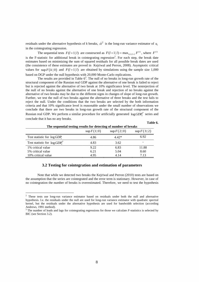
The results are provided in Table 63. The null of no breaks in long-run growth rate of the

structural component of the Russian real GDP against the alternative of one break is failed to reject

but is rejected against the alternative of two break at 10% significance level. The nonrejection of

the null of no breaks against the alternative of one break and rejection of no breaks against the

alternative of two breaks may be due to the different signs in changes of slope of long-run growth.

Further, we test the null of two breaks against the alternative of three breaks and the test fails to

reject the null. Under the conditions that the two breaks are selected by the both information

criteria and that 10% significance level is reasonable under the small number of observations we

conclude that there are two breaks in long-run growth rate of the structural component of the

Russian real GDP. We perform a similar procedure for artificially generated *log tGDP series and

conclude that it has no any breaks.

Table 6.

The sequential testing results for detecting of number of breaks

sup 1| 0F sup 2 | 0F sup 3 | 2F

Test statistic for log tGDP 4.86 4.42* 6.92

Test statistic for *log tGDP 4.83 3.62 -

1% critical value 9.22 6.83 11.88

5% critical value 6.21 5.04 8.60

10% critical value 4.95 4.14 7.13

3.2 Testing for cointegration and estimation of parameters

Note that while we detected two breaks the Kejriwal and Perron (2010) tests are based on

the assumption that the series are cointegrated and the error term is stationary. However, in case of

no cointegration the number of breaks is overestimated. Therefore, we need to test the hypothesis

2 These tests use long-run variance estimator based on residuals under both the null and alternative

hypothesis. I.e. the residuals under the null are used for long-run variance estimator with quadratic spectral

kernel, but the residuals under the alternative hypothesis are used for bandwidth selection (according

Andrews, 1991 method). 3 The number of leads and lags for cointegrating regressions for those we calculate F-statistics is selected by

BIC (see Section 3.2).

9

that the variables are indeed cointegrated provided that we use the estimated number of breaks.

Then if we find evidence of cointegration, the estimated number of breaks is correct.

For cointegration testing the typical approach is to estimate cointegrating regression and

then to test the obtained residuals for stationarity (the presence of cointegration) and/or unit root

(the absence of cointegraton), see Engle and Granger (1987) and MacKinnon (2010).

The presence of structural breaks also affects the results of the tests for cointegration or

no cointegration. For example, if we test the null of no cointegration, this hypothesis will be rarely

rejected if there are breaks in cointegrating regression (see, e.g., Gregory and Hansen, 1996). On

the other hand, the null of cointegration without breaks will be often rejected if the breaks are

actually present in the data (see, e.g., Arai and Kurozumi, 2007 and Carrion-i-Silvestre and Sanso-

i-Rossello, 2006). Here the limiting distributions depend not only on the number of time series but

on the number of structural breaks and the type of them.

For cointegration testing we need to estimate the break dates. Based on minimizing the

sum of squared residuals (assuming that there are two breaks) we obtain the following estimates of

the break dates: 1998Q3 and 2007Q3. The first break date is coincides to the univariate case break

date, but the second break date is shifted to the left to 2007Q3.

After estimation of the break dates we construct the regression

(6) 0 1 1 2 2l ˆ ˆ( )o ( ) ogg l oil

t t t t tt DT T T T p uD DG P ,

and test the residuals ˆtu for a unit root.

Similar to Gregory and Hansen (1996), the unit root test is the conventional ADF test

with appropriate critical values. Stationarity test is the conventional KPSS test (with long-run

variance correction as in Sul et al., 2005) also with appropriate critical values. Asymptotic critical

values are obtained by Monte-Carlo simulations with sample size 1,000 and 20,000 replications.

The results are presented in Table 7. Along with tests for cointegration with two breaks we also

presents the tests for cointegration with no breaks and with only one break. In the latter case, the

break date was estimated by minimizing sum of squared residuals over all possible break dates.

Table 7.

Results for cointegration testing

No cointegration cointegration

No breaks

Test statistic -2.64 0.078

10% critical value -3.49 0.099



One break (2008Q1)

Test statistic -3.95* 0.108**




Two breaks (1998Q3 and 2007Q3)

Test statistic -4.43** 0.033



10


As Table 7 shows, under the assumption of no breaks in long-run growth rate in the

Russian real GDP the null of no cointegration is failed to reject and as well as the null of

cointegration is failed to reject. Nonrejection of the first hypothesis can be due to the low power due to the neglecting breaks. And nonrejection of the second one can be due to the breaks in trend

have different signs in data generating process. In the case of one break the null of no

cointegration is rejected at 10% significance level and the null of cointegration is rejected at 5%

significance level. Thus the testing results were inconsistent with each other which reflecting in

favor of our assumptions about the low power of the stationarity test with different signs of trend

breaks. If we allow two breaks then the results becomes consistent with each other. So the null of

no cointegration is rejected at 5% significance level and the null of cointegration is failed to reject

at any reasonable significance level. Therefore, the formal statistical results allow us to classify the

GDP and oil prices to be cointegrated.

After the cointegration testing we proceed to the estimation of the parameters of

cointegrating regression (6). Note that although the estimator of cointegrating vector

0 1 2( , , , , ) obtained by estimating a reduced rank regression as in Johansen (1991) is

consistent and asymptotically normal, we can obtain the estimates of cointegrating vector based on

regression (6) by OLS. However, in contrast to the Johansen reduced rank regression, the limiting

distribution will be non-pivotal due to the correlation between regressors and error term. So we

cannot use standard inference.

For obtaining pivotal t -statistics alternative methods were developed. The most popular

of them are Dynamic OLS (DOLS) proposed by Saikkonen (1991) and Stock and Watson (1993),

fully-modified OLS (FMOLS) proposed by Phillips and Hansen (1990) and Canonical

Cointegrating Regressions (CCR) proposed by Park (1992)4. Based on these methods we can

obtain standard normal t -tests for cointegrating vector. Although all three methods are

asymptotically equivalent the DOLS is preferred in finite samples (see Carrion-i-Silvestre and

Sanso-i-Rossello, 2006). The method consists in adding the leads and lags of first differences of

repressors and the first differences of regressors.

We estimate parameters of (6) by using DOLS. For lead and lag length selection we use

BIC5, which select the number of leads and lags equal to zero. Thus, it is sufficient to include only

first difference of log oil prices in cointegrating regression. For long-run variance estimation, we

use quadratic spectral kernel with automatic bandwidth selection as in Andrews (1991). The

estimation results are presented in Table 8. It should be noted that the high statistical significance

of the coefficients 1 and

2 that reflect breaks in slopes of trend in the transition from one

regime to the next is the additional evidence of at least two breaks in cointegration regression

model. For coefficients i we make the linear transformation in order to find estimates of growth

rates for particular sample periods in % per year terms (see Table 9).

4 For analytical comparison of these three methods see Kurozumi and Hayakawa (2009). 5 As Choi and Kurozumi (2012) show the BIC is preferable for reducing of mean squared error of

cointegrating vector.

11

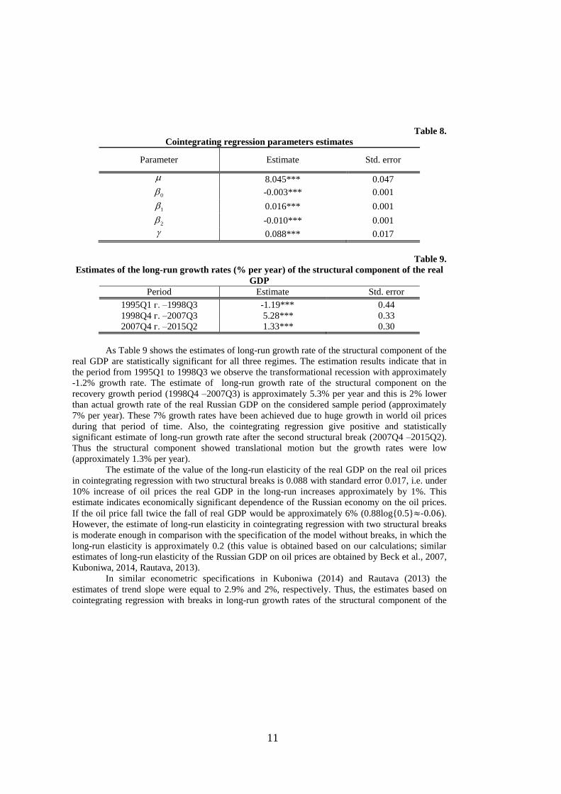
Table 8.

Cointegrating regression parameters estimates

Parameter Estimate Std. error

8.045*** 0.047

0 -0.003*** 0.001

1 0.016*** 0.001

2 -0.010*** 0.001

0.088*** 0.017

Table 9.

Estimates of the long-run growth rates (% per year) of the structural component of the real

GDP

Period Estimate Std. error

1995Q1 г. –1998Q3 -1.19*** 0.44

1998Q4 г. –2007Q3 5.28*** 0.33

2007Q4 г. –2015Q2 1.33*** 0.30

As Table 9 shows the estimates of long-run growth rate of the structural component of the

real GDP are statistically significant for all three regimes. The estimation results indicate that in

the period from 1995Q1 to 1998Q3 we observe the transformational recession with approximately

-1.2% growth rate. The estimate of long-run growth rate of the structural component on the

recovery growth period (1998Q4 –2007Q3) is approximately 5.3% per year and this is 2% lower

than actual growth rate of the real Russian GDP on the considered sample period (approximately

7% per year). These 7% growth rates have been achieved due to huge growth in world oil prices

during that period of time. Also, the cointegrating regression give positive and statistically

significant estimate of long-run growth rate after the second structural break (2007Q4 –2015Q2).

Thus the structural component showed translational motion but the growth rates were low

(approximately 1.3% per year).

The estimate of the value of the long-run elasticity of the real GDP on the real oil prices

in cointegrating regression with two structural breaks is 0.088 with standard error 0.017, i.e. under

10% increase of oil prices the real GDP in the long-run increases approximately by 1%. This

estimate indicates economically significant dependence of the Russian economy on the oil prices.

If the oil price fall twice the fall of real GDP would be approximately 6% (0.88log{0.5}≈-0.06).

However, the estimate of long-run elasticity in cointegrating regression with two structural breaks

is moderate enough in comparison with the specification of the model without breaks, in which the

long-run elasticity is approximately 0.2 (this value is obtained based on our calculations; similar

estimates of long-run elasticity of the Russian GDP on oil prices are obtained by Beck et al., 2007,

Kuboniwa, 2014, Rautava, 2013).

In similar econometric specifications in Kuboniwa (2014) and Rautava (2013) the

estimates of trend slope were equal to 2.9% and 2%, respectively. Thus, the estimates based on

cointegrating regression with breaks in long-run growth rates of the structural component of the

12

GDP during the recovery growth period assign a greater role for the structural component of

economic growth and a less role for the external component.

4 Conclusions

This paper tests existence of structural breaks in the long-run growth rate of the structural

component of the Russian GDP. By the structural component we mean the purified GDP from the

influence of the most important factor of foreign economic conditions of the Russian economy -

oil prices. To solve this problem we use the methodology of cointegrating regression in which we

allow the long-run dependence of the logarithm of the Russian real GDP on the logarithm of the

real oil prices. Also, cointegrating regression equation includes the deterministic linear trend in

which breaks in the slope are allowed (without any level shifts). We treat this term in regression as

the long-run level of the structural component of the GDP.

The empirical results are in favor of the existence of two structural breaks in the long-run

growth rate of the structural component: in the 3rd

quarter of 1998 and in the 3rd

quarter of 2007.

This is evidenced by information criteria and formal statistical tests. According to the estimation

results the long-run growth rate of the structural component is about 5.3% per year during the

recovery growth period (1998Q4 –2007Q3) and about 1.3% per year in subsequent periods. The

output drop in Russia during current economic crisis is in line with the projected reduction due to

the observable oil price decrease. The estimated long-run oil price elasticity of the Russian GDP is

0.088. Thus twofold permanent oil price drop would produce 6% (0.88log{0.5}≈-0.06) decline of

the potential level the Russian GDP.

References

Alquist, R., Kilian, L., Vigfusson, R. J. (2013) Forecasting the price of oil. Handbook of

economic forecasting, 2, pp. 427-507.

Andrews, D.W.K. (1991) Heteroskedasticity and Autocorrelation Consistent Covariance

Matrix Estimation. Econometrica, 59, pp. 817-858.

Arai, Y., Kurozumi, E. (2007) Testing for the Null Hypothesis of Cointegration with a

Structural Break. Econometric Reviews, 26, pp. 705-739.

Aue, A., Horvath, L. (2012) Structural breaks in time series. Journal of Time Series

Analysis, 34, pp. 1-16.

Bai, J., Lumsdaine, R.L., Stock, J.H. (1998) Testing for and Dating Breaks in Integrated

and Cointegrated Time Series. Review of Economic Studies, 65, pp. 395-432.

Bai, J., Perron, P. (1998) Estimating and Testing Linear Models with Multiple Structural

Changes. Econometrica, 66, pp. 47-78.

Bai, J., Perron, P. (2003) Computation and Analysis of Multiple Structural Change Models.

Journal of Applied Econometrics, 18, pp. 1-22.

Beck R., Kamps A., Mileva E. (2007) Long-term growth prospects for the Russian

economy. ECB Occasional Paper. №. 58.

Carrion-i-Silvestre, J.L., Sanso-i-Rossello, A. J. (2005) The KPSS Test with Two Structural

Breaks. Spanish Economic Review, 9, pp. 105-127.

13

Carrion-i-Silvestre, J.L. Sanso-i-Rossello, A. J. (2006) Testing the Null of Cointegration

with Structural Breaks. Oxford Bulletin of Economics and Statistics, 68, pp. 623-646.

Choi, I., Kurozumi, E. (2012) Model selection criteria for the leads-and lags cointegrating

regression. Journal of Econometrics, 169, pp. 224-238.

Drobyshevskij S., Polbin A. (2015) Dekompozicija dinamiki macroekonomicheskih

pokazatelej RF na osnove DSGE-modeli [Decomposition of the Structural Shocks Contribution to

the Russian Macroeconomic Indicators Dynamics on the Basis of the DSGE Model]. Economic

Policy, 2, pp. 20–42.

Engle, R., Granger, C. W. J., (1987) Co-integration and Error Correction: Representation,

Estimation, and Testing. Econometrica, 55, pp. 251-276.

Esfahani H. S., Mohaddes K., Pesaran M. H. (2014) An Empirical Growth Model for Major

Oil Exporters. Journal of Applied Econometrics, 2014, 29, pp. 1-21.

Gregory, A.W., Hansen, B.E. (1996) Residual-based Tests for Cointegration in Models

with Regime Shifts. Journal of Econometrics, 70, pp. 99-126.

Hansen B. E. (1995) Rethinking the univariate approach to unit root testing: using

covariates to increase power // Econometric Theory, 11, pp. 1148-1171.

Harvey, D.I., Leybourne, S.J. (2013) Break Date Estimation for Models with Deterministic

Structural Change. Oxford Bulletin of Economics and Statistics, 76, pp. 623-642.

Harvey, D.I., Leybourne, S.J., Taylor, A.M.R. (2013) Testing for Unit Roots in the Possible

Presence of Multiple Trend Breaks using Minimum Dickey-Fuller Statistics. Journal of

Econometrics, 177, pp. 265-284.

Jandhyala, V., Fotopoulos, S., MacNeill, I., Liu, P. (2016) Inference for single and multiple

change-points in time series. Journal of Time Series Analysis (forthcoming).

Johansen, S., 1991. Estimation and Hypothesis Testing of Cointegration Vectors in

Gaussian Vector Autoregressive Models. Econometrica, 59, pp. 1551-1580.

Idrisov G., Kazakova M., Polbin A. (2015) A theoretical interpretation of the oil prices

impact on economic growth in contemporary Russia. Russian Journal of Economics, 1(3), pp. 257-

272.

Idrisov G., Sinel'nikov-Murylev S. (2014) Formirovanie predposylok dolgosrochnogo

rosta: kak ih ponimat'? [Forming Sources of Long-run Growth: How to Understand Them?]

Voprosy Economiki, 3, pp. 4-20.

Kejriwal, M. (2008) Cointegration with Structural Breaks: An Application to the Feldstein-

Horioka Puzzle. Studies in Nonlinear Dynamics and Econometrics, 12, Article 3.

Kejriwal, M., Perron, P. (2010) Testing for Multiple Structural Changes in Cointegrated

Regression Models. Journal of Business and Economic Statistics, 28, pp. 503-522.

Kuboniwa M. (2014) A Comparative Analysis of the Impact of Oil Prices on Oil–Rich

Emerging Economies in the Pacific Rim. Journal of Comparative Economics, 42, pp. 328-339.

Kudrin A., Gurvich E. (2014) Novaja model' rosta dlja rossijskoj economiki [A New

Growth Model for the Russian Economy]. Voprosy Economiki, 12, pp. 4-36.

Kurozumi, E. (2002) Testing for Stationarity with a Break. Journal of Econometrics, 108,

pp. 63-99.

Kurozumi, E., Hayakawa, K. (2009) Asymptotic properties of the efficient estimators for

cointegrating regression models with serially dependent errors. Journal of Econometrics, 149, pp.

118-135.

Liu, J., Wu S., Zidek, J.V. (1997) On Segmented Multivariate Regressions. Statistica

Sinica, 7, pp. 497-525.

14

MacKinnon, J.G. (2010) Critical values for cointegration tests. QED Working Paper No.

1227.

Mehlum H., Moene K., Torvik R. (2006) Institutions and the resource curse. The Economic

Journal, 116, pp. 1-20.

Park, J. Y. (1992) Canonical Cointegrating Regressions. Econometrica, 60, pp. 119-143.

Perron, P. (2006) Dealing with Structural Breaks. Palgrave Handbooks of Econometrics:

Vol. 1 Econometric Theory, Chapter 8. T. C. Mills and K. Patterson (eds.). Palgrave MacMillan,

Basingstoke., pp. 278-352.

Perron, P., Wada, T. (2009) Let's Take a Break: Trends and Cycles in US Real GDP.

Journal of Monetary Economics, 56, pp. 749-765.

Phillips, P. C. B., Hansen, B. E. (1990) Statistical inference in instrumental variables

regression with I(1) processes. Review of Economic Studies, 57, pp. 99-125.

Rautava J. (2013) Oil Prices, Excess Uncertainty and Trend Growth. Focus on European

Economic Integration, 4, pp. 77-87.

Sachs J.D., Warner A.M. (1997) Fundamental Sources of Long–Run Growth. American

Economic Review, 87, pp. 184-188.

Saikkonen, P. (1991) Asymptotically Efficient Estimation of Cointegration Regression.

Econometric Theory, 7, pp. 1-21.

Skrobotov, A. (2015) On trend breaks and initial condition in unit root testing.

Unpublished manuscript.

Sobreira, N., Nunes, L.C. (2016) Tests for Multiple Breaks in the Trend with Stationary or

Integrated Shocks. Oxford Bulletin of Economics and Statistics (forthcoming).

Stock, J. H., Watson, M. W. (1993) A Simple Estimator of Cointegrating Vectors in Higher

Order Integrated Systems. Econometrica, 61, pp. 783-820.

Sul, D., Phillips, P.C.B., Choi, C. Y. (2005) Prewhitening Bias in HAC Estimation. Oxford

Bulletin of Economics and Statistics, 67, 517- 546.

testing for structural breaks in the long-run growth rate...

Documents