Modelling Regime Switching and Structural Breaks with

an Infinite Dimension Markov Switching Model ∗

Yong SongUniversity of Toronto

tommy.song@utoronto.ca

October 27, 2010

Abstract

This paper proposes an infinite dimension Markov switching model to accommo-date regime switching and structural break dynamics or a combination of both in aBayesian framework. Two parallel hierarchical structures, one governing the transitionprobabilities and another governing the parameters of the conditional data density,keep the model parsimonious and improve forecasts. This nonparametric approachallows for regime persistence and estimates the number of states automatically. Aglobal identification algorithm for structural changes versus regime switching is pre-sented. Applications to U.S. real interest rates and inflation compare the new modelto existing parametric alternatives. Besides identifying episodes of regime switchingand structural breaks, the hierarchical distribution governing the parameters of theconditional data density provides significant gains to forecasting precision.

∗I am sincerely thankful to my supervisor, professor John M. Maheu, for guidance and many helpfulcomments. I am also grateful to Martin Burda, Christian Gourieroux, Thomas McCurdy, Rodney Strachanand seminar attendants at Australian National University and University of Toronto.

1

1 Introduction

This paper contributes to the current literature by accommodating regime switch-

ing and structural break dynamics in a unified framework. Current regime switching

models are not suitable to capture instability of dynamics because they assume finite

number of states and that the future is like the past. Structural break models allow the

dynamics to change over time, however, they may incur loss in the estimation precision

because the past states cannot recur and the parameters in each state are estimated

separately. An infinite dimension Markov switching model is proposed to accommo-

date both types and provide much richer dynamics. The paper shows how to globally

identify structural breaks versus regime switching. In applications to U.S. real interest

rates and inflation, the new model performs better than the alternative parametric

regime switching models and the structural break models in terms of in-sample fit and

out-of-sample forecasts. The model estimation and forecasting are based on a Bayesian

framework.

Regime switching models were first applied by Hamilton (1989) to U.S. GNP data.

It is an important methodology to model nonlinear dynamics and widely applied to eco-

nomic data including business cycles (Hamilton, 1989), bull and bear markets (Maheu

et al., 2010), interest rates (Ang and Bekaert, 2002) and inflation (Evans and Wachtel,

1993). There are two common features of the previous models. First, past states can

recur over time. Second, the number of states is finite (it is usually 2 and at most 4).

In the rest of the paper, a regime switching model is assumed to have both features.

However, the second feature may cause biased out-of-sample forecasts if there exist

sudden changes of the dynamics.

In contrast to the regime switching models, the structural break models can capture

dynamic instability by assuming an infinite or a much larger number of states at the

cost of extra restrictions. For example, Koop and Potter (2007) proposed a structural

break model with an infinite number of states. If there is a change in the data dynamics,

it will be captured by a new state. On the other hand, the restriction in their model

is that the parameters in a new state are different from those in the previous ones. It

is imposed for estimation tractability. However, it prevents the data divided by break

points from sharing the same model parameter, and could incur some loss in estimation

precision. In the current literature, among many, structural break models such as Chib

(1998); Pesaran et al. (2006); Wang and Zivot (2000) and Maheu and Gordon (2008)

have the same feature as Koop and Potter (2007) that the states cannot recur. In the

rest of the paper, a structural break model is assumed to have non-recurring states and

an infinite or a large number of states.

From previous introduction, regime switching and structural break dynamics have

different implications for data fitting and forecasting. However, a method to reconcile

2

them is missing in the current literature. For instance, a common practice is to use

one approach or the other in applications. Levin and Piger (2004) modelled U.S.

inflation as a structural break process while Evans and Wachtel (1993) assumed a

two-regime Markov switching model. Which feature is more important for inflation

analysis, regime switching, structural breaks or both? Garcia and Perron (1996) used

a three-regime Markov switching model for U.S. real interest rates while Wang and

Zivot (2000) applied a model with structural breaks in mean and volatility. Did the

real interest rates in 1981 have distinct dynamics or return to a historical state with the

same dynamics? Existing econometric models have difficulty answering these questions.

This paper provides a solution by proposing an infinite dimension Markov switching

model. It incorporates regime switching and structural break dynamics in a unified

framework. Recurring states are allowed to improve estimation and forecasting preci-

sion. An unknown number of states is embedded in the infinite dimension structure and

estimated endogenously to capture the dynamic instability. Different from the Bayesian

model averaging methodology, this model combines different dynamics nonlinearly.

The proposed model builds on and extends Fox et al. (2008). They used a Dirichlet

process1 as a prior on the transition probabilities of an infinite hidden Markov switching

model. The key innovation in their work is introducing a sticky parameter that favours

state persistence and avoids the saturation of states. Their model is denoted by FSJW

in the rest of the paper. Jochmann (2010) applies FSJW to investigate the structural

breaks in the U.S. inflation dynamics.

The contributions of this paper are as follows. First, a second hierarchical structure

in addition to FSJW is introduced to allow learning and sharing the information for

the parameter of the conditional data density in each state. This approach is labelled

as the sticky double hierarchical Dirichlet process hidden Markov model (SDHDP-

HMM). Second, I present an algorithm to globally define structural breaks versus

regime switching dynamics.2 This is done by avoiding the label switching problem and

focusing on labelling invariant posterior statistics. Last, the paper provides a detailed

comparison of the new SDHDP-HMM against existing alternative regime switching

and structural change models by out-of-sample density forecast through a simulation

study and two empirical applications to U.S. real interest rates and inflation. The

results show that the SDHDP-HMM is robust to model uncertainty and superior in

forecasting and the hierarchical structure on the conditional data density parameters

improves out-of-sample performance significantly.

In the application to U.S. real interest rates, the SDHDP-HMM is compared to the

regime switching model by Garcia and Perron (1996) in a Bayesian framework and the

1The Dirichlet process is a commonly used prior in Bayesian nonparametric models.2Jochmann (2010) proposes to identify structural breaks, but ignores recurring states in the posterior

inference.

3

structural break model by Wang and Zivot (2000) with minor modification. The results

of the SDHDP-HMM supports Garcia and Perron’s (1996) finding of the switching

points at the beginning of 1973 (the oil crisis) and the middle of 1981 (the federal budget

deficit) instead of Huizinga and Mishkin’s (1986) finding of October 1979 and October

1982 (both are monetary policy changes). The SDHDP-HMM also identifies two of the

three turning points found by Wang and Zivot (2000). The model comparison based on

the predictive likelihood shows regime switching dynamics dominates structural break

dynamics for U.S. real interest rates.

The second application is to U.S. inflation. The SDHDP-HMM is compared to the

regime switching model by Evans and Wachtel (1993) in a Bayesian framework and a

structural break model by Chib (1998). This application shows the inflation has both

features of the regime switching and the structural breaks. The SDHDP-HMM can

capture both features and provide richer dynamics than existing parametric models.

The predictive likelihoods further confirm that it is robust to model uncertainty and

superior in forecasting.

The rest of the paper is organized as follows: Section 2 introduces the Dirichlet pro-

cess to make this paper self-contained. Section 3 outlines the sticky double hierarchical

Dirichlet process hidden Markov model and discusses its model structure and impli-

cations. Section 4 sketches the posterior sampling algorithm, explains how to identify

the regime switching and the structural break dynamics, and describes the forecasting

method. Section 5 compares the SDHDP-HMM to regime switching and structural

break models through simulation. Section 6 studies the dynamics of U.S. real inter-

est rate by revisiting the Markov switching model of Garcia and Perron (1996) in the

Bayesian framework and the structural break model of Wang and Zivot (2000) with

minor modification, and comparing them to the SDHDP-HMM using an extended data

set. Section 7 applies the SDHDP-HMM to U.S. inflation, and compares it to Evans

and Wachtel’s (1993) Markov switching model in a Bayesian framework, Chib’s (1998)

structural break model and Fox et al.’s (2008) model. Section 8 concludes.

2 Dirichlet process

Before introducing the Dirichlet process, the definition of the Dirichlet distribution is

the following:

Definition The Dirichlet distribution is denoted by Dir(α), where α is a K-

dimensional vector of positive values. Each sample x from Dir(α) is a K-dimentional

4

vector with xi ∈ (0, 1) andK∑

i=1xi = 1. The probability density function is

p(x | α) =

Γ(K∑

i=1αi)

K∏

i=1Γ(αi)

K∏

i=1

xαi−1i

A special case is the Beta distribution denoted by B(α1, α2), which is a Dirichlet

distribution with K = 2.

Define α0 =K∑

i=1αi, Xi, the ith element of the random vector X from a Dirichlet

distribution Dir(α), has mean αi

α0and variance αi(α0−αi)

α2

0(α0+1)

. Hence, we can further de-

compose α into two parts: a shape parameter G0 = (α1

α0, · · · , αK

α0) and a concentration

parameter α0. The shape parameter G0 represents the center of the random vector X

and the concentration parameter α0 controls how close X is to G0.

The Dirichlet distribution is conjugate to the multimonial distribution in the fol-

lowing sense: if

X ∼ Dir(α)

β = (n1, . . . , nK) | X ∼ Mult(X)

where ni is the number of occurrences of i in a sample of n =K∑

i=1ni points from the

discrete distribution on 1, · · · , K defined by X, then

X | β = (n1, . . . , nK) ∼ Dir(α + β)

This relationship is used in Bayesian statistics to estimate the hidden parameters X,

given a collection of n samples. Intuitively, if the prior is represented as Dir(α), then

Dir(α + β) is the posterior following a sequence of observations with histogram β.

The Dirichlet process was introduced by Ferguson (1973) as the extension of the

Dirichlet distribution from finite dimension to infinite dimension. It is a distribution

of distributions and has two parameters: the shape parameter G0 is a distribution over

a sample space Ω and the concentration parameter α0 is a positive scalar. They have

similar interpretation as their counterparts in the Dirichlet distribution. The formal

definition is the following:

Definition The Dirichlet process over a set Ω is a stochastic process whose sample

path is a probability distribution over Ω. For a random distribution F distributed

according to a Dirichlet process DP(α0, G0), given any finite measurable partition

5

A1, A2, · · · , AK of the sample space Ω, the random vector (F (A1), · · · , F (AK)) is dis-

tributed as a Dirichlet distribution with parameters (α0G0(A1), · · · , α0G0(AK)).

Use the results form the Dirichlet distribution, for any measurable set A, the random

variable F (A) has mean G0(A) and variance G0(A)(1−G0(A))α0+1 . The mean implies the

shape parameter G0 represents the centre of a random distribution F drawn from

a Dirichlet process DP(α0, G0). Define ai ∼ F as an observation drawn from the

distribution F . Because by definition P (ai ∈ A | F ) = F (A), we can derive P (ai ∈ A |

G0) = E(P (ai ∈ A | F ) | G0) = E(F (A) | G0) = G0(A). Hence, the shape parameter

G0 is also the marginal distribution of an observation ai. The variance implies the

concentration parameter α0 controls how close the random distribution F is to the

shape parameter G0. The larger α0 is, the more likely F is close to G0, and vice versa.

Suppose there are n observations, a = (a1, · · · , an), drawn from the distribution

F . Usen∑

i=1δai

(Aj) to represent the number of ai in set Aj , where A1, · · · , AK is a

measurable partition of the sample space Ω and δai(Aj) is the Dirac measure, where

δai(Aj) =

1 if ai ∈ Aj

0 if ai /∈ Aj

Conditional on (F (A1), · · · , F (AK)), the vector

(

n∑

i=1δai

(A1), · · · ,n∑

i=1δai

(AK)

)

has a

multinomial distribution. By the conjugacy of Dirichlet distribution to the multimo-

mial distribution, the posterior distribution of (F (A1), · · · , F (AK)) is still a Dirichlet

distribution

(F (A1), · · · , F (AK)) | a ∼ Dir

(

α0G0(A1) +n∑

i=1

δai(A1), · · · , α0G0(AK) +

n∑

i=1

δai(AK)

)

Because this result is valid for any finite measurable partition, the posterior of F is

still Dirichlet process by definition, with new parameters α∗0 and G∗

0, where

α∗0 = α0 + n

G∗0 =

α0

α0 + nG0 +

n

α0 + n

n∑

i=1

δai

n

The posterior shape parameter, G∗0, is the mixture of the prior and the empirical

distribution implied by observations. As n → ∞, the shape parameter of the posterior

converges to the empirical distribution. The concentration parameter α∗0 → ∞ implies

the posterior of F converges to the empirical distribution with probability one. Fergu-

son (1973) showed that a random distribution drawn from a Dirichlet process is almost

6

sure discrete, although the shape parameter G0 can be continuous. Thus, the Dirichlet

process can only be used to model continuous distributions with approximation.

For a random distribution F ∼ DP(α0, G0), because F is almost surely discrete,

it can be represented by two parts: different values θi’s and their corresponding prob-

abilites pi’s, where i = 1, 2, · · · . Sethuraman (1994) found the stick breaking rep-

resentation of the Dirichlet process by writing F ≡ (θ, p), where θ ≡ (θ1, θ2, · · · )′,

p ≡ (p1, p2, · · · )′ with pi > 0 and

∞∑

i=1pi = 1. The F ∼ DP(α0, G0) can be generated by

Viiid∼ Beta(1, α0) (1)

pi = Vi

i−1∏

j=1

(1 − Vj) (2)

θiiid∼ G0 (3)

where i = 1, 2, · · · . In this representation, p and θ are generated independently. The

process generating p, (1) and (2), is called the stick breaking process. The name comes

after the pi’s generation. For each i, the remaining probability, 1−i−1∑

j=1pj , is sliced by a

proportion of Vi and given to pi. It’s like breaking a stick an infinite number of times.

This paper uses the notation p ∼ SBP(α0) for this process.

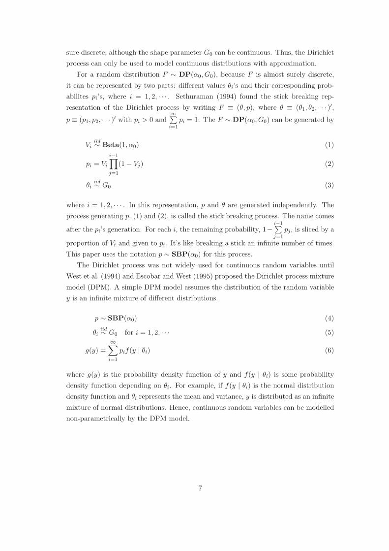
The Dirichlet process was not widely used for continuous random variables until

West et al. (1994) and Escobar and West (1995) proposed the Dirichlet process mixture

model (DPM). A simple DPM model assumes the distribution of the random variable

y is an infinite mixture of different distributions.

p ∼ SBP(α0) (4)

θiiid∼ G0 for i = 1, 2, · · · (5)

g(y) =∞∑

i=1

pif(y | θi) (6)

where g(y) is the probability density function of y and f(y | θi) is some probability

density function depending on θi. For example, if f(y | θi) is the normal distribution

density function and θi represents the mean and variance, y is distributed as an infinite

mixture of normal distributions. Hence, continuous random variables can be modelled

non-parametrically by the DPM model.

7

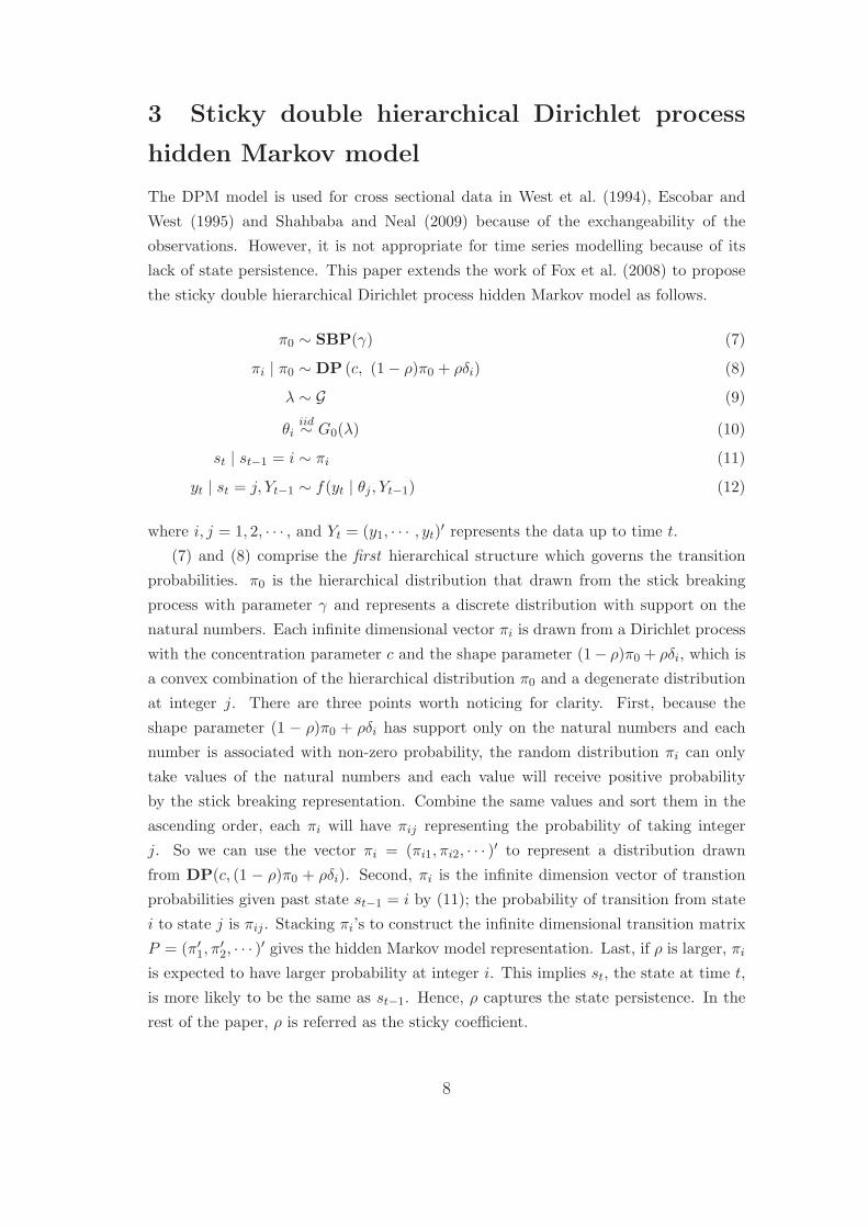
3 Sticky double hierarchical Dirichlet process

hidden Markov model

The DPM model is used for cross sectional data in West et al. (1994), Escobar and

West (1995) and Shahbaba and Neal (2009) because of the exchangeability of the

observations. However, it is not appropriate for time series modelling because of its

lack of state persistence. This paper extends the work of Fox et al. (2008) to propose

the sticky double hierarchical Dirichlet process hidden Markov model as follows.

π0 ∼ SBP(γ) (7)

πi | π0 ∼ DP (c, (1 − ρ)π0 + ρδi) (8)

λ ∼ G (9)

θiiid∼ G0(λ) (10)

st | st−1 = i ∼ πi (11)

yt | st = j, Yt−1 ∼ f(yt | θj , Yt−1) (12)

where i, j = 1, 2, · · · , and Yt = (y1, · · · , yt)′ represents the data up to time t.

(7) and (8) comprise the first hierarchical structure which governs the transition

probabilities. π0 is the hierarchical distribution that drawn from the stick breaking

process with parameter γ and represents a discrete distribution with support on the

natural numbers. Each infinite dimensional vector πi is drawn from a Dirichlet process

with the concentration parameter c and the shape parameter (1− ρ)π0 + ρδi, which is

a convex combination of the hierarchical distribution π0 and a degenerate distribution

at integer j. There are three points worth noticing for clarity. First, because the

shape parameter (1 − ρ)π0 + ρδi has support only on the natural numbers and each

number is associated with non-zero probability, the random distribution πi can only

take values of the natural numbers and each value will receive positive probability

by the stick breaking representation. Combine the same values and sort them in the

ascending order, each πi will have πij representing the probability of taking integer

j. So we can use the vector πi = (πi1, πi2, · · · )′ to represent a distribution drawn

from DP(c, (1 − ρ)π0 + ρδi). Second, πi is the infinite dimension vector of transtion

probabilities given past state st−1 = i by (11); the probability of transition from state

i to state j is πij . Stacking πi’s to construct the infinite dimensional transition matrix

P = (π′1, π

′2, · · · )

′ gives the hidden Markov model representation. Last, if ρ is larger, πi

is expected to have larger probability at integer i. This implies st, the state at time t,

is more likely to be the same as st−1. Hence, ρ captures the state persistence. In the

rest of the paper, ρ is referred as the sticky coefficient.

8

(9) and (10) comprise the second hierarchical structure which governs the parame-

ters of the conditional data density. G0(λ) is the hierarchical distribution from which

the state dependent parameter θi is drawn independently; G is the prior of λ. This

structure provides a way of learning λ from past θi’s to improve estimation and fore-

casting. If a new state is born, the conditional data density parameter θnew is drawn

from G0(λ). Without the second hierarchical structure, the new draw θnew depends

on some assumed prior. Pesaran et al. (2006) argued the importance of modelling

the hierarchical distribution for the conditional data density parameters in the pres-

ence of structural breaks. This paper adopts their method to estimate the hierarchical

distribution G0(λ).

In comparison to the SDHDP-HMM, FSJW is comprised of (7)-(8) and (10)-(12).

The stick breaking representation of the Dirichlet process is not fully explored by

FSJW, since it has only one hierarchical structure on the transition probabilities. In

fact, the stick breaking representation (1)-(3) decomposes the generation of a distri-

bution F from a Dirichlet process into two independent parts: the probabilities are

generated from a stick breaking process and the parameter values are generated from

the shape parameter independently. The SDHDP-HMM takes full advantage of this

structure than FSJW by modelling two parallel hierarchical structures.

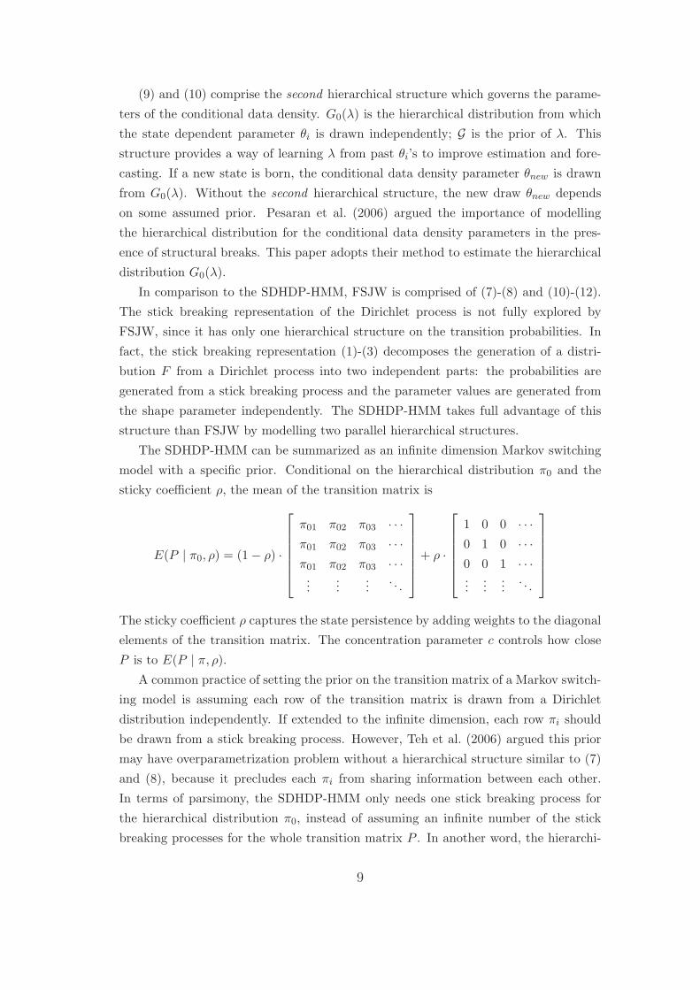
The SDHDP-HMM can be summarized as an infinite dimension Markov switching

model with a specific prior. Conditional on the hierarchical distribution π0 and the

sticky coefficient ρ, the mean of the transition matrix is

E(P | π0, ρ) = (1 − ρ) ·

π01 π02 π03 · · ·

π01 π02 π03 · · ·

π01 π02 π03 · · ·...

......

. . .

+ ρ ·

1 0 0 · · ·

0 1 0 · · ·

0 0 1 · · ·...

......

. . .

The sticky coefficient ρ captures the state persistence by adding weights to the diagonal

elements of the transition matrix. The concentration parameter c controls how close

P is to E(P | π, ρ).

A common practice of setting the prior on the transition matrix of a Markov switch-

ing model is assuming each row of the transition matrix is drawn from a Dirichlet

distribution independently. If extended to the infinite dimension, each row πi should

be drawn from a stick breaking process. However, Teh et al. (2006) argued this prior

may have overparametrization problem without a hierarchical structure similar to (7)

and (8), because it precludes each πi from sharing information between each other.

In terms of parsimony, the SDHDP-HMM only needs one stick breaking process for

the hierarchical distribution π0, instead of assuming an infinite number of the stick

breaking processes for the whole transition matrix P . In another word, the hierarchi-

9

cal structure on the transition probabilities collapses setting the prior on the infinite

dimension matrix P to the infinite dimension vector π0.

The SDHDP-HMM is also related to the DPM model (4)-(6), because (12) can be

replaced by

yt | st−1 = i, Yt−1 ∼∞∑

j=1

πijf(yt | θj , Yt−1) (13)

On one hand, the DPM representation implies the SDHDP-HMM is nonparametric.

On the other hand, different from the DPM model, the mixture probability πij is state

dependent. This feature allows the SDHDP-HMM to capture time varying dynamics.

In summary, the SDHDP-HMM is an infinite state space Markov switching model

with a specific form of prior to capture state persistence. Two parallel hierarchical

structures are proposed to provide parsimony and improve forecasting. It preserves the

nonparametric methodology of the DPM model but has state dependent probabilities

on its mixture components.

4 Estimation, inference and forecasting

In the following simulation study and applications, the conditional dynamics yt |

θj , Yt−1 in (12) is set as Gaussian AR(q) process.

yt | θj , Yt−1 ∼ N(φj0 + φj1yt−1 + · · · + φjqyt−q, σ2j )

By definition, the conditional data density parameter θi = (φ′i, σi)

′ with φi = (φi0, φi1, · · · , φiq)′.

The hierarchical distribution G0(λ) in (10) is assumed as the regular normal-gamma

distribution in the Bayesian literature.3 The conditional data density parameter θi is

generated as follows:

σ−2i ∼ G (χ/2, ν/2) , φi | σi ∼ N

(

φ, σ2i H

−1)

(14)

By definition, λ = (φ, H, χ, ν). φ is a (q +1)×1 vector, H is a (q +1)× (q +1) positive

definite matrix, and χ and ν are positive scalars. It is a standard conjugate prior for

linear models. Precision parameter σ−2i is drawn from a gamma distribution with de-

gree of freedom ν/2 and multiplier χ/2. Given the hierarchical distribution parameter

λ, the conditional mean and variance of σ−2i are ν/χ and 2ν/(χ)2, respectively. And

φi | σi is drawn from a multivariate normal distribution with mean φ and covariance

matrix σ2i H

−1.

3For example, see Geweke (2009).

10

The prior on the hierarchical parameters λ in (9) follows Pesaran et al. (2006).

H ∼ W(A0, a0) (15)

φ | H ∼ N(m0, τ0H−1) (16)

χ ∼ G(d0/2, c0/2) (17)

ν ∼ Exp(ρ0) (18)

H is drawn from a Wishart distribution with parameters of a (q + 1)× (q + 1) positive

definite matrix A0 and a positive scalar a0. Samples from this distribution are positive

definite matrices. The expected value of H is A0a0. The variance of Hij , the ith row

and jth colomn element of H, is a0(A2ij + AiiAij), where Aij is the ith row and jth

colomn element of A0. m0 is a (q + 1) × 1 vector representing the mean of φ and τ0 is

a positive scalar controls the prior belief of the dispersion of φ. χ is distributed as a

gamma distribution with the multiplier d0/2 and the degree of freedom c0/2. ν has an

exponential distribution with parameter ρ0,

The posterior sampling is based on Markov chain Monte Carlo (MCMC) methods.

Fox et al. (2008) showed the sampling scheme of FSJW. The block sampler based

on approximation by a finite number of states is more efficient than the individual

sampler.4

In order to apply the block sampler following Fox et al. (2008), the SDHDP-HMM

is approximated by a finite number of states proposed as follows.

π0 ∼ Dir( γ

L, · · · ,

γ

L

)

(19)

πi | π0 ∼ Dir ((1 − ρ)cπ01, ..., (1 − ρ)cαπ0i + ρc, · · · , (1 − ρ)cπ0L) (20)

λ ∼ G (21)

θiiid∼ G0(λ) (22)

st | st−1 = i ∼ πi (23)

yt | st = j, Yt−1 ∼ N(φj0 + φj1yt−1 + · · · + φjqyt−q, σ2j ) (24)

where L is the maximal number of states in the approximation and i = 1, 2, · · · , L. The

hierarchical distribution G0(λ) and its prior are set as (14) and (15)-(18), respectively.

From the empirical point of view, the essence of the SDHDP-HMM is not only its

infinite dimension, but also its sensible hierarchical structure of the prior. If L is large

enough, the finite approximation (19)-(24) is equivalent to the original model (7)-(12)

in practice.

4Consistency of the approximation was proved by Ishwaran and Zarepour (2000), Ishwaran and Zarepour(2002). Ishwaran and James (2001) compared the individual sampler with the block sampler and found thelater one is more efficient in terms of mixing.

11

4.1 Estimation

Appendix A shows the detailed posterior sampling algorithm. The parameter space

is partitioned into four parts: (S, I), (Θ, P, π0), (φ, H, χ) and ν. S, I and Θ are the

collections of st, a binary auxiliary variable It and θi, respectively.5 Each part is

sampled conditional on the other parts and the data Y as follows.

1. Sample (S, I) | Θ, P, Y

(a) Sample S | Θ, P, Y by the forward and backward smoother in Chib (1996).

(b) Sample I | S by a Polya Urn scheme.

2. Sample (Θ, P, π0) | S, I, Y

(a) Sample Θ | S, Y by regular linear model result.

(b) Sample π0 | I by a Dirichlet distribution.

(c) Sample P | π0, S by Dirichlet distributions.

3. Sample (φ, H, χ) | S, Θ, ν

(a) Sample (φ, H) | S, Θ by conjugacy of the Normal-Wishart distribution.

(b) Sample χ | ν, S, Θ by a gamma distribution.

4. Sample ν | χ, S,Θ by a Metropolis-Hastings algorithm.

After initiate the parameter values, the algorithm is applied iteratively by many

times to obtain a large sample of the model parameters. Discard the first block of

the samples to remove dependence on the initial values. The rest of the sample,

S(i), Θ(i), P (i), π(i)0 , φ(i), H(i), χ(i), ν(i)N

i=1, are used for inferences as if they were drawn

from the posterior distribution. Simulation consistent posterior statistics are computed

as sample averages. For example, the posterior mean of φ, E(φ | Y ), is calculated by1N

∑Ni=1 φ(i).

Fox et al. (2008) did not consider the label switching problem, which is an issue in

mixture models.6 For example, switching the values of (θj , πj) and (θk, πk), swapping

the values of state st for st = j, k while keeping the other parameters unchanged

will result in the same likelihood value in the finite approximation of the SDHDP-

HMM. Inference on a label dependent statistic such as θj is misleading without extra

constraints. Geweke (2007) showed that inappropriate constraints can also result in

misleading inferences. To identify regime switching and structural breaks, this paper

uses label invariant statistics. So the posterior sampling algorithm can be implemented

without modification as suggested by Geweke (2007).

5It is an auxiliary variable for sampling of π0. The details are in the appendix A.6See Celeux et al. (2000), Fruhwirth-Schnatter (2001) and Geweke (2007)

12

4.2 Identification of regime switching and structural breaks

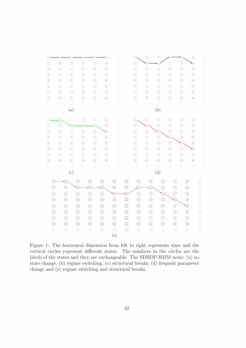
A heuristic illustration of how a SDHDP-HMM nests different dynamics including

regime switching and structural breaks is plotted in figure 1. Each path comprised by

arrows is one sample path of state S in a SDHDP-HMM. Figure 1a represents the no

state change case (the Gaussian AR(q) model from the assumption). Figure 1b-1d are

regime switching, structural break and frequent parameter change case, respectively.

Figure 1e captures more complicated dynamics, in which some states are only visited

for one consecutive period while others are not.

The current literature does not study the identification of regime switching and

structural breaks in the infinite dimension Markov switching models. This paper

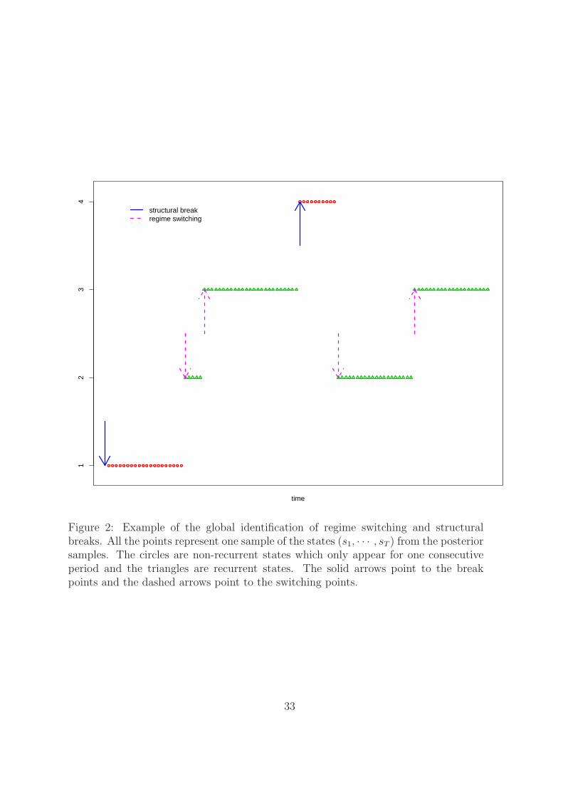
proposes a global identification algorithm to identify regime switching and structural

breaks based on whether a state is recurrent or not. In detail, if a state only appears

for one consecutive period, it is classified as a non-recurrent state. Otherwise, it is de-

fined as recurrent. The starting time of a recurrent (non-recurrent) state is identified

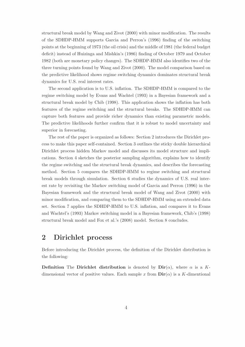
as a regime switching (structural break) point. In figure 2, state 1 and 4 with circles

are non-recurrent states and the starting points of these two segments are identified as

structural breaks. State 2 and 3 with triangles are recurrent states, and the starting

time of each consecutive periods are identified as regime switching points.

In detail, if there exist time t0 and t1 (without loss of generality, let t0 ≤ t1) such

that st = j if and only if t0 ≤ t ≤ t1, then state j is non-recurrent and t0 is identified

as a break point. On the other hand, if st0 6= st0−1 and t0 is not a break point, then t0

is identified as a regime switching point.

This identifcation criteria is simply because, in general, states are recurrent in the

regime switching models but non-recurrent in the structural break ones. There are

two points worth noticing. First, in terms of mathematical statistics, a recurrent (non-

recurrent) state in a Markov chain is defined as a state which will be visited with

probability one (less than one) in the future. This paper defines the recurrence (non-

recurrence) as a statistic on one realized posterior sample path of the state variable S.

Because the mathematical definition is not applicable to the estimation with a finite

sample size, there should be no confusion between these two concepts. Second, a true

path of states from a regime switching model can have non-recurrent states because

of randomness or a small sample size. For example, state 2, 3 and 4 in figure 2 can

be generated from a three-regime switching model. The algorithm identifies state 4

as a non-recurrent states, and its starting point is classified as a break point. Hence,

this identification approach may label a switching point of a regime switching model

as a structural break even if the true states were observed. However, this is simply

accidental. As more data are observed, an embedded regime switching model will have

all its states identified as recurrrent.

13

More importantly, the purpose of the identification is not to decompose the infinite

dimension Markov switching model into several regime switching and structural break

sub-models (there is no unique way even if we wanted to), but to study the richer

dynamics which allow recurrent states while accommodating structural breaks. Even

if a non-recurrent state was generated from a regime switching model, it usually has

different implication from the recurrent states of the same model.

Hence, separating the recurrent and non-recurrent states is both empirically reason-

able and theoretically consistent with the definition of regime switching and structural

breaks of the existing respective models. In the rest of the paper, the SDHDP-HMM

associates regime switching and structural breaks to recurrent and non-recurrent states.

4.3 Forecast and model comparison

Predictive likelihood is used to compare the SDHDP-HMM to the existing regime

switching and structural break models. It is similar to the marginal likelihood by Kass

and Raftery (1995). Conditional on an initial data set Yt, the predictive likelihood of

Y Tt+1 = (yt+1, · · · , yT ) by model Mi is calculated as

p(Y Tt+1 | Yt, Mi) =

T∏

τ=t+1

p(yτ | Yτ−1, Mi) (25)

It is equivalent to the marginal likelihood p(YT | Mi) if t = 0.

The calculation of one-period predictive likelihood of model Mi, p(yt | Yt−1, Mi), is

p(yt | Yt−1, Mi) =1

N

N∑

i=1

f(yt | Υ(i), Yt−1, Mi) (26)

where Υ(i) is one sample of parameters from the posterior distribution conditional on

the historical data Yt−1. For the SDHDP-HMM, (26) is

p(yt | Yt−1) =1

N

N∑

i=1

L∑

k=1

π(i)jk f(yt | θ

(i)k , s

(i)t−1 = j, Yt−1)

After the calculation of the one-period predictive likelihood, p(yt | Yt−1), the data is

updated by adding one observation, yt, and the model is re-estimated for the prediction

of the next period. This is repeated until the last predivtive likelihood, p(yT | YT−1),

is obtained.

Kass and Raftery (1995) compared model Mi and Mj by the difference of their

log marginal likelihood log(BFij) = log(Y | Mi) − log(Y | Mj). They suggested

interpreting the evidence for Mi versus Mj as: not worth more than a bare mention for

14

0 ≤ log(BFij) < 1; positive for 1 ≤ log(BFij) < 3; strong for 3 ≤ log(BFij) < 5; and

very strong for log(BFij) ≥ 5. BFij is referred as the Bayes factor of Mi versus Mj .

This paper uses this criteria for model comparison by predictive likelihood. Geweke

and Amisano (2010) showed the interpretation is the same as Kass and Raftery (1995)

if we regard the initial data Yt as a training sample.

5 Simulation evidence

To investigate how the SDHDP-HMM reconciles the regime switching and the struc-

tural break models, this section provides some simulation evidence based on three

models: the SDHDP-HMM, a finite Markov switching model, and a structural break

model. Each model simulates a data set of 1000 observations, and all three data sets are

estimated by a SDHDP-HMM with the same prior. First, I plot the posterior means of

the conditional data density parameters E(θst | YT ) and the true values θst over time.

If the SDHDP-HMM fits the model well, the posterior means are supposed to be close

to the true ones. Second, more rigorous study is based on the predictive likelihoods.

Each of the 3 models is estimated on each of the 3 simulated data sets. The last 100

observations are used to calculate the predictive likelihood. If the SDHDP-HMM is

able to accommodate the other two models, its predictive likelihood based on the data

simulated from the alternative model should be close to the predictive likelihood es-

timated by the true model; and if the SDHDP-HMM provides richer dynamics than

the other two models, its predictive likelihood based on the data simulated from the

SDHDP-HMM should strongly dominates the predictive likelihoods calculated by the

other two models.

The parameters of the SDHDP-HMM in simulation are set as: γ = 3, c = 10, ρ =

0.9, χ = 2, ν = 2, φ = 0 and H = I. The number of AR lags is set as 2. The simulation

is done through the Polya-Urn scheme without approximation as in Fox et al. (2009).

The simulated data are plotted in figure 3.

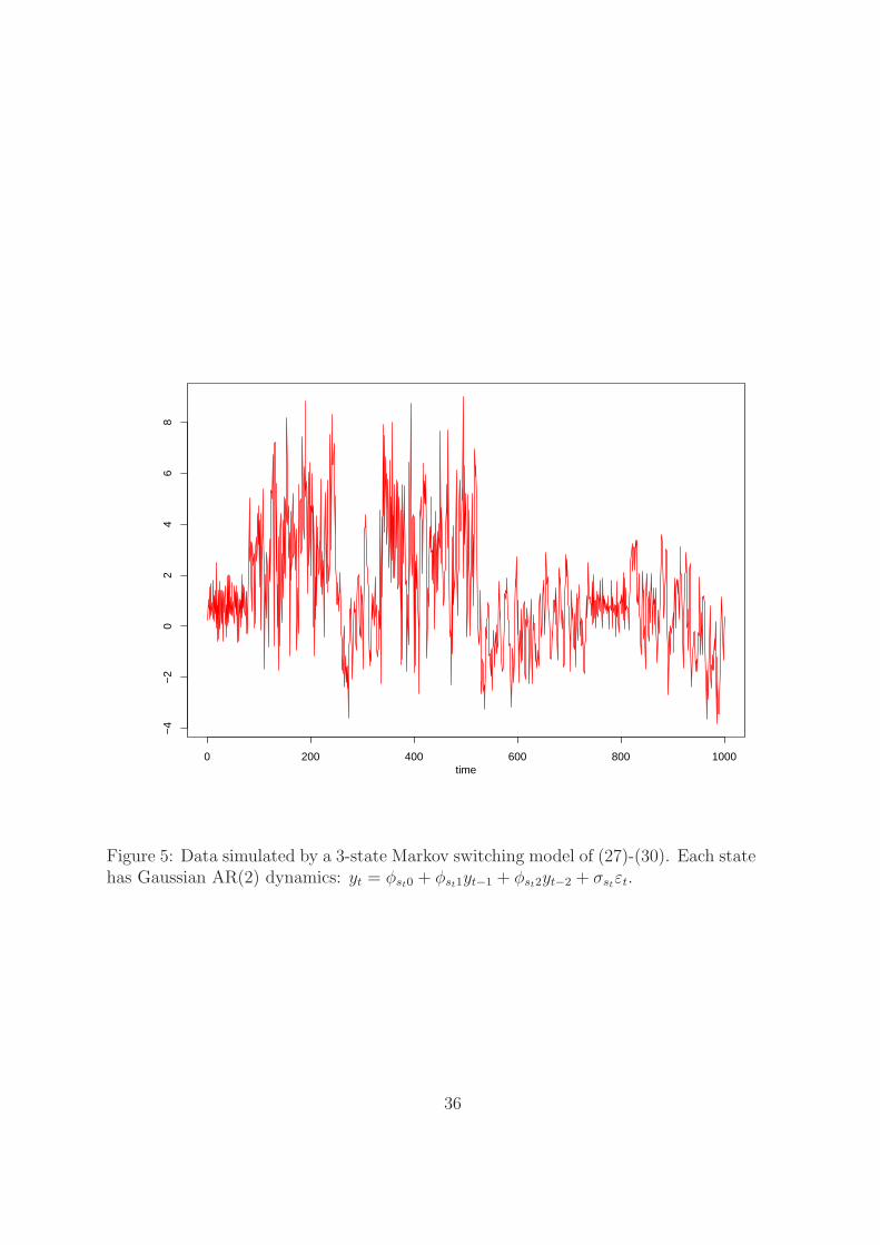
The first competitor is a K-state Markov switching model as follows:

(pi1, · · · , piK) ∼ Dir(ai1, · · · , aiK) (27)

(φi, σi)iid∼ G0 (28)

Pr(st = j | st−1 = i) = pij (29)

yt | st = j, Yt−1 ∼ N(φj0 + φj1yt−1 + · · · + φjqyt−q, σ2j ) (30)

where i, j = 1, · · · , K. Each AR process uses 2 lags as in the SDHDP-HMM. The num-

ber of states, K, is set as 3. Conditional data density parameters are φ1 = (0, 0.8, 0),

φ2 = (1,−0.5, 0.2), φ3 = (2, 0.1, 0.3) and (σ1, σ2, σ3) = (1, 0.5, 2). The transition ma-

15

trix is set as P =

0.96 0.02 0.02

0.02 0.96 0.02

0.02 0.02 0.96

. The simulated data are plotted in figure 5. The

prior of each row of the transition matrix, (pj1, · · · , pjK), is set as independent dirichlet

distribution Dir(1, · · · , 1). The prior of the conditional data density parameters G0 is

set as the normal-gamma distribution, where σ−2i ∼ G (1, 1) and φi | σi ∼ N

(

0, σ2i I)

.

The second competitor is a K-state structural break model of Chib (1998):

p ∼ B(ap, bp) (31)

Pr(st = i | st−1 = i) =

p if i < K

1 if i = K(32)

Pr(st = i + 1 | st−1 = i) = 1 − p if i < K (33)

(φi, σi)iid∼ G0 for i = 1, · · · , K (34)

yt | st = i, Yt−1 ∼ N(φi0 + φi1yt−1 + · · · + φiqyt−q, σ2k) (35)

where i = 1, 2, · · · , K is the state indicator. The break probability 1 − p and the

number of AR lags are set as 0.003 and 2, respectively. In simulation, the K = 4 and

the parameters of the conditional data density are φ1 = (0, 0.8, 0), φ2 = (1,−0.5, 0.2),

φ3 = (0.5, 0.1, 0.3), φ4 = (0, 0.5, 0.2) and (σ1, σ2, σ3, σ4) = (1, 0.5, 1, 0.5). The simulated

data are plotted in figure 8. K = 5 is used in estimation to nest the true data generating

process. The prior of p is set as a beta distribution B(9, 1), and G0 is set the same as

the Markov switching model of (28).

All of the three simulated data sets are estimated by the SDHDP-HMM. The param-

eters γ, c, ρ and the number of AR lags are set the same as in the SDHDP-HMM used in

simulation. The maximal number of states, L, is assumed as 10. The priors on the other

parameters are weakly informative as follows: H ∼ W(0.2I, 5), φ | H ∼ N(0, H−1),

χ ∼ G(0.5, 0.5) and ν ∼ Exp(1).

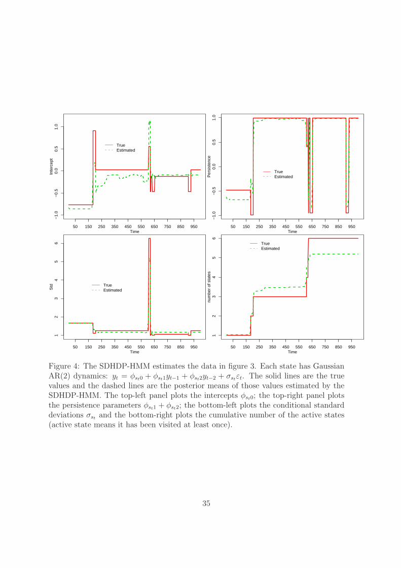
The intercept, the persistence parameter (sum of AR coefficients), the standard

deviation and the cumulative number of active states of the simulated data from the

SDHDP-HMM over time are plotted in figure 4 by solid lines. The posterior means

of those parameters from the estimation are also plotted for comparison in the same

figure by dashed lines. Without surprise, the estimated values tracks the true ones

closely and sharply identifies the change points. Because the estimation is based on

the finite approximation while the simulation is by the true data generating process,

the results support the validity of the block sampler.

Figure 6 plots the true values of the intercept, the persistence, the volatility and

the cumulative number of switching of the simulated data from the Markov switching

model over time by solid lines, together with the posterior means of these parameters

16

estimated from the SDHDP-HMM by dashed lines. Figure 7 plots the true and the

posterior mean of the regime switching and structural break probabilities implied by the

SDHDP-HMM. The SDHDP-HMM sharply identifies almost all the switching points.

From the middle panel, the global identification does not find prominent strauctural

breaks.

Figure 9 plots the true parameters from the data simulated from the structural

break model by solid lines and the posterior mean of those parameters estimated from

the SDHDP-HMM by dashed lines. Again, the SDHDP-HMM tracks different pa-

rameters closely. Figure 10 plots the true and the posterior mean of the structural

break and regime switching probabilities. The SDHDP-HMM identifies all the break

points. The bottom panel shows some small probabilities of regime switching around

the structural break points. Those values are very small comparing to the structural

break probabilities.

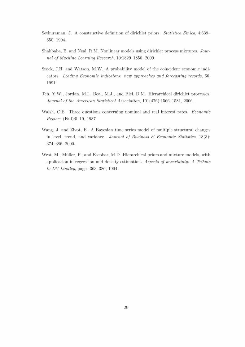
A more rigorous model comparison is in table 1. It shows the log predictive likeli-

hoods of the last 100 observations estimated by all of the above three models on all of

the three simulated data sets. The SDHDP-HMM is robust to model misspecification

because it’s not strongly rejected against the true model by the log predictive likeli-

hoods. For example, if the true data generating process is the Markov switching model,

the log predictive likelihoods computed by the true model and the SDHDP-HMM are

−208.10 and −208.32, respectively. The difference is only −208.10−(−208.32) = 0.22 <

1 and not worth more than a bare mention. On the other hand, both the Markov switch-

ing model and the structural break model are strongly rejected if the other one is the

true model. For example, if the structural break model is the data generating process,

the log predictive likelihoods calculate by the true model and the Markov switching

model are −178.41 and −187.26. Their difference is −178.41 − (−187.26) = 8.85 > 5,

which is very strong against the misspecified model.

Besides the robustness, the SDHDP-HMM is also able to capture more complicated

dynamics than the Markov switching model and the structural break model. If the

SDHDP-HMM is the true data generating process, the Markov switching model and

the structural break model are both rejected strongly. The log predictive likelihood of

the SDHDP-HMM is 12.75 larger than the Markov switching model and 91.4 larger

than the structural break model. Both values are greater than 5.

In summary, the simulation evidence shows the SDHDP-HMM is robust to model

uncertainty. Both of the Markov switching model and the structural break model can

be tracked closely. Meanwhile, SDHDP-HMM provides richer dynamics than the other

two types of models.

17

6 Application to U.S. real interest rate

The first application is to U.S. real interest rate. Previous studies by Fama (1975); Rose

(1988) and Walsh (1987) tested the stability of their dynamics. While Fama (1975)

found the ex ante real interest rate as a constant, Rose (1988) and Walsh (1987) cannot

reject the existence of an integrated component. Garcia and Perron (1996) reconciled

these results by a three-regime Markov switching model and found switching points

at the beginning of 1973 (the oil crisis) and the middle of 1981 (the federal budget

deficit) using quarterly U.S. real interest rates of Huizinga and Mishkin (1986) from

1961Q1-1986Q3. The real interest rate dynamics in each state are characterized by an

Gaussian AR(2) process. Wang and Zivot (2000) used the same data to investigate

structural breaks and found support of four states (3 breaks) by Bayes factors.

This paper constructs U.S. quarterly real interest rate in the same way as Huizinga

and Mishkin (1986) and extends their data set to a total of 252 observations from

1947Q1 to 2009Q4. The last 200 observations are used for predictive likelihood cal-

culation. Alternative models for comparison include the Markov switching model of

Garcia and Perron (1996) put in a Bayesian framework, the structural break model

of Wang and Zivot (2000) with minor modification and linear AR models. All but

the linear model have the Gaussian AR(2) process in each state as Garcia and Perron

(1996) and Wang and Zivot (2000).

The priors of the SDHDP-HMM are set as follows:

π0 ∼ Dir(1/L, · · · , 1/L)

πi | π0 ∼ Dir(π01, · · · , π0i + 9, · · · , π0L)

H ∼ W(0.2 I, 5)

φ | H ∼ N(0, H−1)

χ ∼ G(0.5, 2.5)

ν ∼ Exp(5)

where i = 1, · · · , L. The block sampler uses the truncation of L = 10.7

The Markov switching model used is (27)-(30). Garcia and Perron (1996) estimated

the model in the classical approach and this paper revisits their paper in the Bayesian

framework. The prior of each row of the transition matrix, (pi1, · · · , piK), is set as

Dir(1, · · · , 1). The priors of φi and σi are σ−2i ∼ G(2.5, 0.5) and φi | σi ∼ N(0, σ2

i · I).

The structural break model is (31)-(35). This paper allows simultaneous break of

the intercept, the AR coefficients and the volatility, while Wang and Zivot (2000) only

7L = 10 is chosen to represent a potentially large number of states and keep a reasonable amount ofcomputation. Some larger L’s are also tried and produce similar results.

18

allowed the intercept and the volatility to change. The prior of p is a beta distribution

B(9, 1), and parameters φi and σi have the same priors as the Markov switching model.

A linear AR model is applied as a benchmark for model comparison.

(φ, σ) ∼ G0 (36)

yt | Yt−1 ∼ N(φ0 + φ1yt−1 + · · · + φqyt−q, σ2) (37)

where the prior of σ is set the same as in the Markov switching model and the structural

break model. The prior of φ | σ is N(0, σ2 · I), where the dimension of vector 0 and

the identity matrix I depends on the number of lags q in the AR model.

Table 2 shows the log predictive likelihoods of different models. First, all linear

models are dominated by nonlinear models. Second, the log predictive likelihoods

strongly support the Markov switching models against structural break models. The

log predictive likelihood of four-regime or five-regime Markov switching model is larger

than that of any K-regime structural break models by more than 5, which is very

strong based on Kass and Raftery (1995). Last, although the SDHDP-HMM does not

strongly dominate the Markov switching models, it still performs the best among all

the models. This is consistent with the simulation evidence that the SDHDP-HMM

can provide robust forecasts by optimally combining regime switching and structural

breaks in the Bayesian framework.

The whole sample is estimated by the SDHDP-HMM with the same prior in the

predictive likelihood calculation. Figure 11 plots the posterior mean of different pa-

rameters over time, including the regime switching and structural break probabilities.

There is no sign of structural breaks from the bottom panel, so the regime switching

dynamics prevail over the structural break dynamics, which is consistent with table 2

based on the predictive likelihoods. Three important regimes are found in the figure,

one has high volatility and high persistence, one has low volatility and intermediate

persistence and the last one has intermediate volatility and low persistence.

Define a state to be active if it is occupied by some data. Figure 12 plots the

posterior mean of the cumulative number of active states over time. The posterior

mean of the total number of active states is 3.4. Compared to the truncation of L = 10

in the estimation, this value implies the finite truncation restriction is not binding, so

the nonparametric flavor is preserved.

Garcia and Perron (1996) found switching points at the beginning of 1973 and

the middle of 1981. In the SDHDP-HMM, the probability of regime switching in

1973Q1 is 0.39, which is consistent with their finding. From 1980Q2 to 1981Q1, the

probabilities of regime switching are 0.18, 0.13, 0.32 and 0.19, respectively. There are

many uncertainties in the switching point identification at these times. However, it

is quite likely that the state changed in one of these episodes, which is only slightly

19

earlier than in Garcia and Perron (1996). On the other hand, Huizinga and Mishkin

(1986) identified October 1979 and October 1982 as the turning points. Probabilities

of regime switching or structural breaks in 1979Q3 and Q4 are less than 0.02 and

0.04 respectively, while in 1982Q3 and 1982Q4 they are both less than 0.01. Thus,

the SDHDP-HMM supports Garcia and Perron (1996) against Huizinga and Mishkin

(1986).

As an attempt to locate potential state changing points, I define a time with the

sum of regime switching and structural break probability greater than 0.3 as a candi-

date turning point. There are 9 points in total: 1952Q1, 1952Q3, 1956Q2, 1958Q2,

1973Q1, 1980Q4, 1986Q2, 2002Q1, 2005Q3. Among those points, 1973Q1, 1980Q4

are consistent with Garcia and Perron (1996). Wang and Zivot (2000) found 1970Q3,

1980Q2 and 1985Q4 as structural break points. 1980Q4 and 1986Q2 are close to their

finding. However, the SDHDP-HMM does not identify late 1970 as neither a break nor

a switching point, which contradicts their result.

In summary, by using a larger sample, U.S. real interest rates are better described

by a regime switching model than a structural break one. The robustness of the

SDHDP-HMM to model uncertainty is supported by the predictive likelihoods. The

SDHDP-HMM performs better than all the parametric alternatives in forecasting.

7 Application to U.S. inflation

The second application is to the U.S. inflation. Ang et al. (2007) studied the perfor-

mance of different methods including time series models, Phillips curve based models,

asset pricing models and surveys. The regime switching model is the best in their most

recent sub-sample. Evans and Wachtel (1993) applied a two-regime Markov switching

model to explain consistent inflation forecast bias. Their model incorporated a random

walk model of Stock and Watson (1991) in one regime and a stationary AR(1) model in

another. Structural breaks in inflation were studied by Groen et al. (2009); Levin and

Piger (2004) and Duffy and Engle-Warnick (2006). Application of the SDHDP-HMM

can reconcile these two types of models and provide more description of the inflation

dynamics.

Monthly inflation rates are constructed from U.S. Bureau of Labor Statistics based

on CPI-U. There are 1152 observations from Feb 1914 to Jan 2010. It is computed

as annualized monthly CPI-U growth rate scaled by 100. The alternative models

for comparison include the FSJW, the regime switching model of Evans and Wachtel

(1993), a structural break model of Chib (1998) and linear Gaussian AR(q) model.

For the SDHDP-HMM, each state has Gaussian AR(1) dynamics. L = 10 and the

20

priors are

π0 ∼ Dir(1/L, · · · , 1/L)

πi | π0 ∼ Dir(π01, · · · , π0i + 9, · · · , π0L)

H ∼ W(0.2 I, 5)

φ | H ∼ N(0, H−1)

χ ∼ G(0.5, 2.5)

ν ∼ Exp(5)

with i = 1, · · · , L.

In FSJW, each state has Gaussian AR(1) dynamics and the number of states L = 10

as the SDHDP-HMM to use the block sampler. The priors of the transition probabilities

are the same as the SDHDP-HMM. The prior on the parameters of conditional data

density is normal-gamma: σ−2i ∼ G(0.5, 0.5) and φi | σi ∼ N(0, σ2

i I).

For comparison, the structural break model of (31)-(35) is also applied with the

number of the AR lags equal to 1. The prior of p is a beta distribution B(9, 1); and

the priors of φi and σi are the same as FSJW.

Another alternative model is the regime switching model of Evans and Wachtel

(1993):

P (st = i | st−1 = i) = pi

(φ0, σ0) ∼ G0

σ1 ∼ G1

yt | st = 0, Yt−1 ∼ N(φ00 + φ01yt−1, σ20)

yt | st = 1, Yt−1 ∼ N(yt−1, σ21)

where i = 1, 2. The prior of the self-transition probability, pi, is a beta distribution

B(9, 1). φ0, σ0, and σ1 have the same priors as FSJW and the structural break model.

The linear AR model of (36) and (37) is applied as a benchmark for model compar-

ison. The prior of σ is set the same as in FSJW, the Markov switching model and the

structural break model. The prior of φ | σ is N(0, σ2 · I), where the dimension of the

vector 0 and the identity matrix I depends on the number of lags q in the AR model.

The last 200 observations are used to calculate the log predictive likelihoods. The

results are shown in table 3. First, the linear models are strongly dominated by the

nonlinear models. Second, the regime switching model of Evans and Wachtel (1993)

strongly dominates the structural break models. Thrid, FSJW strongly dominates all

the other parametric alternatives including the regime switching model. The difference

21

between the log predictive likelihoods of FSJW and the regime switching model is

−82.45 − (−92.50) = 6.05, which implies heuristically FSJW is exp(6.05) ≈ 424 times

better than Evans and Wachtel (1993) model. Last, The SDHDP-HMM is the best

model in terms of the log predictive likelihood. The difference of the log likelihoods of

the SDHDP-HMM and FSJW is −74.07− (−82.45) = 8.38, which implies the SDHDP-

HMM is exp(8.34) ≈ 4188 times better than FSJW. Because the SDHDP-HMM nest

the parametric alternatives, its dominance can be attributed to the fact that both the

regime switching and the structural break dynamics are important for inflation, and

each single type of the parametric model can not capture its dynamics alone.

The models are estimated on the whole sample. The posterior summary statistics

are in table 4. The posterior mean of the persistence parameter is 0.97 with 95% density

interval of (0.742, 1.199), which implies the inflation dynamics are likely to be persistent

in a new state. On the other hand, FSJW draws the parameters of the conditional data

density for each new state from the prior assumption. This key difference contributes

to the superior forecasting ability of the SDHDP-HMM to FSJW.

The smoothed mean of conditional data density parameters, break probabilities

and switching probabilities over time for the SDHDP-HMM are in figure 13. The

instability of the dynamics is consistent with Jochmann (2010). The last panel plots

the structural breaks and regime switching probabilities at different times. There are

2 major breaks at 1920-07 and 1930-05. The structural break and regime switching

probability of 1920-07 are 0.3 and 0.5, respectively. There is a quite large chance for

this time to have unique dynamics than the other periods. For 1930-05, the structural

break and regime switching probability are 0.13 and 0.09. This implies if the state

changed at this time, it is more likely to be a structural break.

To illustrate the dominance of the regime switching dynamics over the structural

break dynamics, figure 14 plots the probabilities of past states to be the same as

the last period, Jan 2010, or p(zτ = z201001 | Y ). Most of the positive probabilities

are before 1955. This emphasizes the importance of modelling recurrent states in

forecasting. Structural break models perform worse than the SDHDP-HMM and the

regime switching model because they drop much useful information.

Figure 15 plots the smoothed regression coefficients, standard deviations and break

probabilities over time estimated by the structural break model with K = 10. Struc-

tural breaks happened in the first half of the sample, therefore the recent regime switch-

ing implied by the SDHDP-HMM is not identified.

Figure 16 plots the smoothed probabilities of in the random walk state and the

smoothed volatility estimated by the regime switching model of Evans and Wachtel

(1993) over time. The random walk dynamics dominate after 1953. In recent times,

inflation dynamics entered into the stationary AR(1) state. This is consistent with

22

the SDHDP-HMM in figure 14 that the most recent episodes are associated with data

before 1955. In another word, there is a regime switching back to the same state in

the past.

In figure 17, all regime switching and structural break probabilities are plotted

for comparison. The first panel is the regime switching model; the second panel is

the structural break model and the last is the SDHDP-HMM. Two features can be

summarized from the figure. First, the change points identified by the structural break

model and the regime switching model are associated with the change points identified

by the SDHDP-HMM. Second, the SDHDP-HMM estimates more turning points than

each of the alternative models. This implies it captures some dynamics that can not be

identified by the regime switching or the structural break model alone. Together with

the log predictive likelihood results in table 3, the inflation has both regime switching

and structural break features.

In summary, the regime switching and the structural break dynamics are both

important for inflation modelling and forecasting. The SDHDP-HMM is able to cap-

ture both of the features. In the SDHDP-HMM, the parameters of the conditional

data density in each state can provide information for the learning of the hierarchical

distribution G0(λ) and improve forecasting significantly.

8 Conclusion

This paper proposes to apply an infinite dimension Markov switching model labelled as

the sticky double hierarchical Dirichlet process hidden Markov model (SDHDP-HMM)

to accommodate regime switching and structural break dynamics. Two parallel hierar-

chical structures, one governing the transition probabilities and the other governing the

parameters of the conditional data density, are imposed for parsimony and to improve

forecasts. An algorithm for global identification of regime switching and structural

breaks is proposed based on label invariant statistics. A simulation study shows the

SDHDP-HMM is robust to model uncertainty and able to capture more complicated

dynamics than the regime switching and the structural break models.

Applications to U.S. real interest rates and inflation show the SDHDP-HMM is

robust to model uncertainty and provides better forecasts than the regime switching

and the structural break models. The second hierarchical structure on the data density

parameters provides significant improvement in inflation forecasting. From both the

predictive likelihood results and the posterior probabilities of regime switching and

structural breaks, U.S. real interest rates are better described by a regime switching

model while the inflation has both features of regime switching and structural breaks.

23

A Block sampling

A.1 Sample (S, I) | Θ, P, Y

S | Θ, P, Y is sampled by the forward and backward smoother in Chib (1996).

I is introduced to facilitate the π0 sampling. From (19) and (20), the filtered

distribution of πi conditional on St = (s1, · · · , st) and π0 is a Dirichlet distribution.

πi | St, π0 ∼ Dir(

c(1 − ρ)π01 + n(t)i1 , · · · , c(1 − ρ)π0i + cρ + n

(t)ii , · · · , c(1 − ρ)π0L + n

(t)iL

)

where n(t)ij is the number of τ | sτ = j, sτ−1 = i, τ ≤ t. Integrate out πi, the

conditional distribution of st+1 given St and π0 is

p(st+1 = j | st = i, St, π0) ∝ c(1 − ρ)π0j + cρδi(j) + n(t)ij

Construct a variable It with a Bernoulli distribution

p(It+1 | st = i, St, π0) ∝

cρ +L∑

j=1n

(t)ij if It+1 = 0

c(1 − ρ) if It+1 = 1

Construct the conditional distribution

p(st+1 = j | It+1 = 0, st = i, St, β) ∝ n(t)ij + cρδi(j)

p(st+1 = j | It+1 = 1, st = i, St, β) ∝ π0j

This construction preserves the same conditional distribution of st+1 given St and

π0. To sample I | S, use the Bernoulli distribution

It+1 | st = i, st+1 = j, π0 ∼ Ber(c(1 − ρ)π0j

n(t)ij + cρδi(j) + c(1 − ρ)π0j

)

A.2 Sample (Θ, P, π0) | S, I, Y

After sampling I and S, write mi =∑

st=iIt. By construction, the conditional posterior

of π0 given S and I only depends on I and is a Dirichlet distribution by conjugacy.

π0 | S, I ∼ Dir(γ

L+ m1, . . . ,

γ

L+ mL)

This approach of sampling π0 is simpler than Fox et al. (2009).

24

Conditional on π0 and S, the sampling of πi is straightforward by conjugacy.

πi | π0, S ∼ Dir(c(1−ρ)π01 +ni1, · · · , c(1−ρ)π0i + cρ+nii, · · · , c(1−ρ)π0L +niL)

where nij is the number of τ | sτ = j, sτ−1 = i.

Sampling Θ | S, Y uses the results of regular linear models. The prior is

(φi, σ−2i ) ∼ N − G(φ, H, χ, ν)

By conjugacy, the posterior is

(φi, σ−2i ) | S, Y ∼ N − G(φi, H i, χi, νi)

with

φi = H−1i (Hφ + X ′

iYi)

H i = H + X ′iXi

χi = χ + Y ′i Yi + φ′Hφ − φ

′Hφ

νi = ν + ni

where Yi is the collection of yt in state i. xt = (1, yt−1, · · · , yt−q) is the regressor in

the AR(q) model. Xi and ni are the collection of xt and the number of observations

in state i, respectively.

A.3 Sample (φ, H, χ) | S, Θ, ν

The conditional posterior is

φ, H | φi, σiKi=1 ∼ N − W(m1, τ1, A1, a1)

where K is the number of active states. φi and σi are the parameters associated with

these states.

m1 =1

τ−10 +

K∑

i=1σ−2

i

(

τ−10 m0 +

K∑

i=1

σ−2i φi

)

τ1 =1

τ−10 +

K∑

i=1σ−2

i

25

A1 =

(

A−10 +

K∑

i=1

σ−2i φiφ

′i + τ−1

0 m0m′0 − τ−1

1 m1m′1

)−1

a1 = a0 + K

The conditional posterior of χ is

χ | ν, σiKi=1 ∼ G(d1/2, c1/2)

with d1 = d0 +K∑

i=1σ−2

i and c1 = c0 + Kν.

A.4 Sample ν | χ, S, Θ

The conditional posterior of ν has no regular density form.

p(ν | χ, σiKi=1) ∝

(

(χ/2)ν/2

Γ(ν/2)

)K ( K∏

i=1

σ−2i

)ν/2

exp−ν

ρ0

Metroplolis-Hastings method is applied to sample ν. Draw a new ν from a proposal

distribution.

ν | ν ′ ∼ G(ζν

ν ′, ζν)

with acceptance probability min

1,p(ν|χ,σi

Ki=1

)fG(ν′; ζνν

,ζν)

p(ν′|χ,σiKi=1

)fG(ν; ζνν′

,ζν)

, where ν ′ is the value from

the previous sweep. ζν is fine tuned to produce a reasonable acceptance rate around

0.5 as suggested by Roberts et al. (1997) and Muller (1991).

References

Ang, A. and Bekaert, G. Regime switches in interest rates. Journal of Business &

Economic Statistics, 20(2):163–182, 2002.

Ang, A., Bekaert, G., and Wei, M. Do macro variables, asset markets, or surveys

forecast inflation better? Journal of Monetary Economics, 54(4):1163–1212, 2007.

Celeux, G., Hurn, M., and Robert, C.P. Computational and Inferential Difficulties with

Mixture Posterior Distributions. Journal of the American Statistical Association, 95

(451), 2000.

Chib, S. Calculating posterior distributions and modal estimates in Markov mixture

models. Journal of Econometrics, 75(1):79–97, 1996.

26

Chib, S. Estimation and comparison of multiple change-point models. Journal of

Econometrics, 86(2):221–241, 1998.

Duffy, J. and Engle-Warnick, J. Multiple regimes in US monetary policy? A nonpara-

metric approach. Journal of Money Credit and Banking, 38(5):1363, 2006.

Escobar, MD and West, M. Bayesian density estimation and inference using mixtures.

Journal of the American Statistical Association, 90, 1995.

Evans, M. and Wachtel, P. Inflation regimes and the sources of inflation uncertainty.

Journal of Money, Credit and Banking, pages 475–511, 1993.

Fama, E.F. Short-term interest rates as predictors of inflation. The American Economic

Review, 65(3):269–282, 1975.

Ferguson. A bayesian analysis of some nonparametric problem. The Annals of Statis-

tics, 1(2):209–230, 1973.

Fox, E.B., Sudderth, E.B., Jordan, M.I., and Willsky, A.S. An HDP-HMM for sys-

tems with state persistence. In Proceedings of the 25th international conference on

Machine learning, pages 312–319. ACM, 2008.

Fox, E.B., Sudderth, E.B., Jordan, M.I., and Willsky, A.S. The Sticky HDP-HMM:

Bayesian Nonparametric Hidden Markov Models with Persistent States. Arxiv

preprint arXiv:0905.2592, 2009.

Fruhwirth-Schnatter, S. Markov Chain Monte Carlo Estimation of Classical and Dy-

namic Switching and Mixture Models. Journal of the American Statistical Associa-

tion, 96(453), 2001.

Garcia, R. and Perron, P. An analysis of the real interest rate under regime shifts. The

Review of Economics and Statistics, 78(1):111–125, 1996.

Geweke, J. Interpretation and inference in mixture models: Simple MCMC works.

Computational Statistics & Data Analysis, 51(7):3529–3550, 2007.

Geweke, J. Complete and Incomplete Econometric Models. Princeton Univ Pr, 2009.

Geweke, J. and Amisano, G. Comparing and evaluating Bayesian predictive distribu-

tions of asset returns. International Journal of Forecasting, 2010.

Groen, J.J.J., Paap, R., and Ravazzolo, F. Real-time inflation forecasting in a changing

world. http://hdl.handle.net/1765/16709, 2009.

27

Hamilton, J.D. A new approach to the economic analysis of nonstationary time series

and the business cycle. Econometrica: Journal of the Econometric Society, 57(2):

357–384, 1989.

Huizinga, J. and Mishkin, F.S. Monetary policy regime shifts and the unusual behavior

of real interest rates, 1986.

Ishwaran, H. and James, L.F. Gibbs Sampling Methods for Stick-Breaking Priors.

Journal of the American Statistical Association, 96(453), 2001.

Ishwaran, H. and Zarepour, M. Markov chain Monte Carlo in approximate Dirichlet

and beta two-parameter process hierarchical models. Biometrika, 87(2):371, 2000.

Ishwaran, H. and Zarepour, M. Dirichlet prior sieves in finite normal mixtures. Statis-

tica Sinica, 12(3):941–963, 2002.

Jochmann, M. Modeling U S Inflation Dynamics: A Bayesian Nonparametric Ap-

proach. Working Paper Series, 2010.

Kass, R.E. and Raftery, A.E. Bayes factors. Journal of the American Statistical

Association, 90(430), 1995.

Koop, G. and Potter, S.M. Estimation and forecasting in models with multiple breaks.

Review of Economic Studies, 74(3):763, 2007.

Levin, A.T. and Piger, J.M. Is inflation persistence intrinsic in industrial economies?

2004.

Maheu, J.M. and Gordon, S. Learning, forecasting and structural breaks. Journal of

Applied Econometrics, 23(5):553–584, 2008.

Maheu, J.M., McCurdy, T.H., and Song, Y. Components of bull and bear markets:

bull corrections and bear rallies. Working Papers, 2010.

Muller, P. A generic approach to posterior integration and Gibbs sampling. Rapport

technique, pages 91–09, 1991.

Pesaran, M.H., Pettenuzzo, D., and Timmermann, A. Forecasting time series subject

to multiple structural breaks. Review of Economic Studies, 73(4):1057–1084, 2006.

Roberts, GO, Gelman, A., and Gilks, WR. Weak convergence and optimal scaling

of random walk Metropolis algorithms. The Annals of Applied Probability, 7(1):

110–120, 1997.

Rose, A.K. Is the real interest rate stable? Journal of Finance, 43(5):1095–1112, 1988.

28

Sethuraman, J. A constructive definition of dirichlet priors. Statistica Sinica, 4:639–

650, 1994.

Shahbaba, B. and Neal, R.M. Nonlinear models using dirichlet process mixtures. Jour-

nal of Machine Learning Research, 10:1829–1850, 2009.

Stock, J.H. and Watson, M.W. A probability model of the coincident economic indi-

cators. Leading Economic indicators: new approaches and forecasting records, 66,

1991.

Teh, Y.W., Jordan, M.I., Beal, M.J., and Blei, D.M. Hierarchical dirichlet processes.

Journal of the American Statistical Association, 101(476):1566–1581, 2006.

Walsh, C.E. Three questions concerning nominal and real interest rates. Economic

Review, (Fall):5–19, 1987.

Wang, J. and Zivot, E. A Bayesian time series model of multiple structural changes

in level, trend, and variance. Journal of Business & Economic Statistics, 18(3):

374–386, 2000.

West, M., Muller, P., and Escobar, M.D. Hierarchical priors and mixture models, with

application in regression and density estimation. Aspects of uncertainty: A Tribute

to DV Lindley, pages 363–386, 1994.

29

Table 1: Log predictive likelihoods in simulation study

DGP Estimated Model

SDHDP-HMM MS SB

SDHDP-HMM -170.55 -183.30 -264.65

MS -208.32 -208.10 -212.07

SB -179.51 -187.26 -178.41

The SDHDP-HMM is (7)-(12); the MS is the 3-state markovswitching model of (27)-(30); and the SB is the 4-statestructural break model of (31)-(35). 1000 observations aresimulated from each model and the last 100 are used tocalculate the predictive likelihoods. The first column showthe names of the data generating processes. The first rowshow the names of the estimated models.

Table 2: Log predictive likelihoods of U.S. real interest rates

AR(q) q=2 q=3 q= 4

-457.62 -451.07 -455.97

MS(K)b K=3 K=4 K=5

-433.09 -426.62 -424.51

SB(K)c K=3 K=4 K=5 K=10 K=15 K=20

-450.82 -451.62 -437.28 -433.50 -432.69 -434.24

SDHDP-HMMe -423.50

There are 252 observations from 1947Q1 to 2009Q4 for U.S. quarterly realinterest rate. The last 200 observations are used to calculate the predictivelikelihoods. MS(K) is the K-state Markov switching model of (27)-(30) andSB(K) is the K-state structural break model of (31)-(35). For theSDHDP-HMM, MS(K) and SB(K), each state has Gaussian AR(2) dynamics.

30

Table 3: Log predictive likelihoods of U.S. inflationa

AR(q) q=1 q=2 q= 3

-185.06 -173.17 -173.42

MS b -92.50

SB(K)c K=3 K=5 K=10

-125.50 -98.69 -101.18

FSJWd -82.45

SDHDP-HMMe -74.07

There are 1153 observations from Feb 1914 to Jan 2010 forU.S. monthly inflation rate. The last 200 observations areused to calculate the predictive likelihoods. MS is the 2-stateMarkov switching model of Evans and Wachtel (1993); SB(K)is the K-state structural break model of (31)-(35); and theFSJW is Fox et al.’s (2008) model (or the SDHDP-HMMwithout the hierarchical structure of G0 on the conditionaldata density parameters). For the SDHDP-HMM, FSJW, MSand SB(K), each state has Gaussian AR(1) dynamics.

Table 4: Posterior summary of theSDHDP-HMM parameters estimatedfrom U.S. inflation

mean Std 95% DI

φ0 0.03 0.20 (-0.376, 0.432)

φ1 0.97 0.11 (0.742, 1.199)

H00 0.77 0.42 (0.225, 1.788)

H01 0.02 0.35 (-0.692, 0.734)

H11 2.06 0.84 (0.768, 4.047)

χ 0.19 0.12 (0.034, 0.488)

ν 1.21 0.50 (0.496, 2.414)

There are 1153 observations from Feb1914 to Jan 2010 for U.S. monthlyinflation rate. Each state has GaussianAR(1) dynamics:yt = φst0

+ φst1yt−1 + σst

εt. Theparameters φi and σi are drawn from thehierarchical distribution:σ−1

i∼ G(χ/2, ν/2) and

φi | σi ∼ N(φ, σiH−1).

31

3

5

6

7

8

2

4

1

3

5

6

7

8

2

4

1

3

5

6

7

8

2

4

1

3

5

6

7

8

2

4

1

3

5

6

7

8

2

4

1

3

5

6

7

8

2

4

1

3

5

6

7

8

2

4

1

(a)

3

5

6

7

8

2

4

1

3

5

6

7

8

2

4

1

3

5

6

7

8

2

4

1

3

5

6

7

8

2

4

1

3

5

6

7

8

2

4

1

3

5

6

7

8

2

4

1

3

5

6

7

8

2

4

1

(b)

3

5

6

7

8

2

4

1

3

5

6

7

8

2

4

1

3

5

6

7

8

2

4

1

3

5

6

7

8

2

4

1

3

5

6

7

8

2

4

1

3

5

6

7

8

2

4

1

3

5

6

7

8

2

4

1

(c)

3

5

6

7

8

2

4

1

3

5

6

7

8

2

4

1

3

5

6

7

8

2

4

1

3

5

6

7

8

2

4

1

3

5

6

7

8

2

4

1

3

5

6

7

8

2

4

1

3

5

6

7

8

2

4

1

(d)

3

5

6

7

8

2

4

1

3

5

6

7

8

2

4

1

3

5

6

7

8

2

4

1

3

5

6

7

8

2

4

1

3

5

6

7

8

2

4

1

3

5

6

7

8

2

4

1

3

5

6

7

8

2

4

1

3

5

6

7

8

2

4

1

3

5

6

7

8

2

4

1

3

5

6

7

8

2

4

1

3

5

6

7

8

2

4

1

3

5

6

7

8

2

4

1

3

5

6

7

8

2

4

1

3

5

6

7

8

2

4

1

(e)

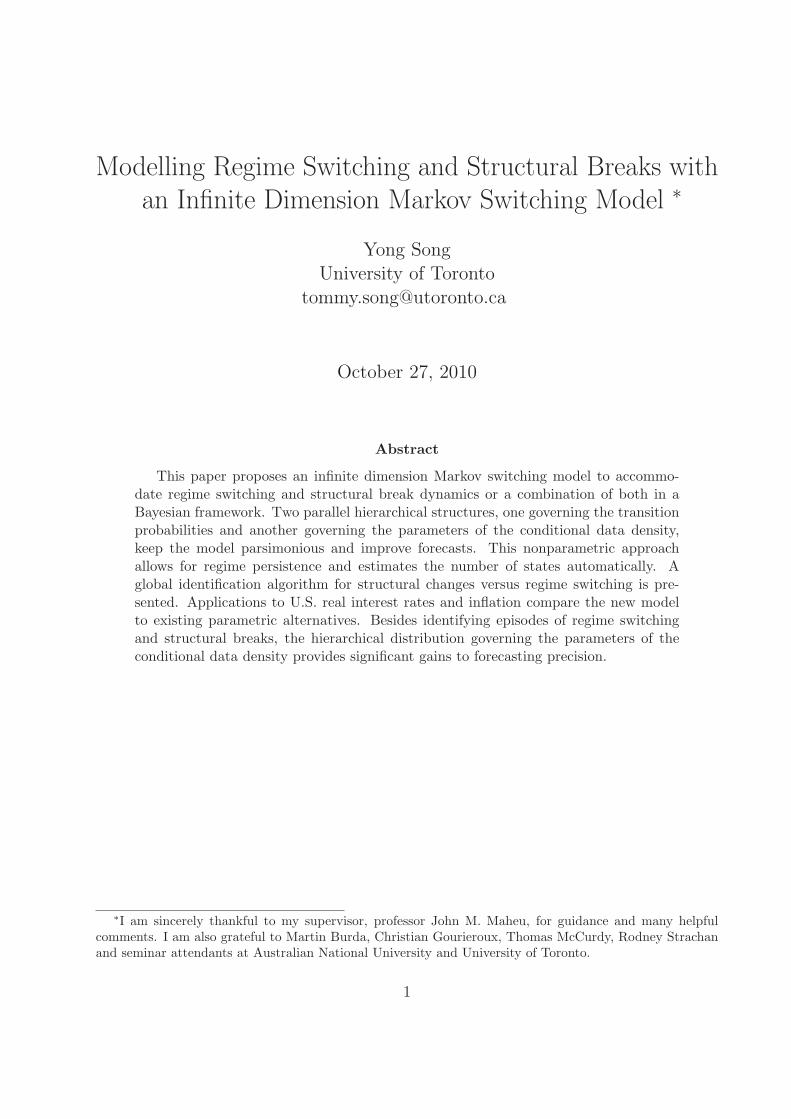
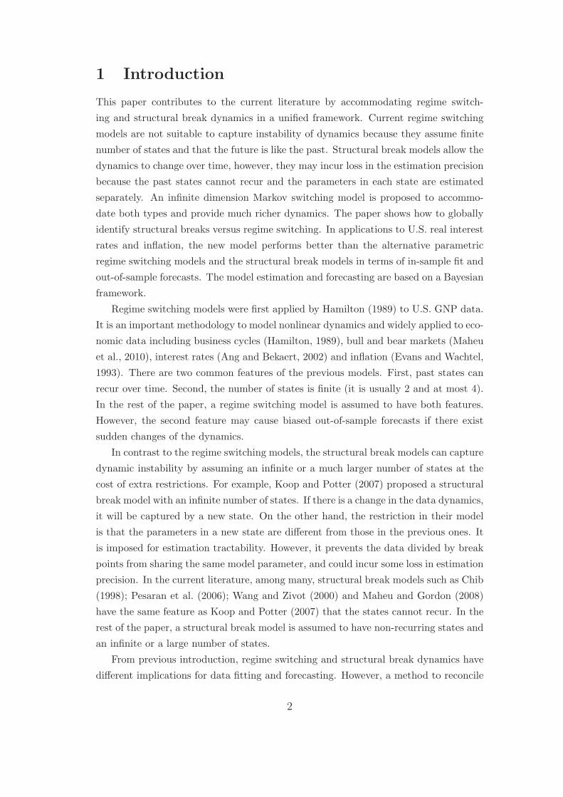
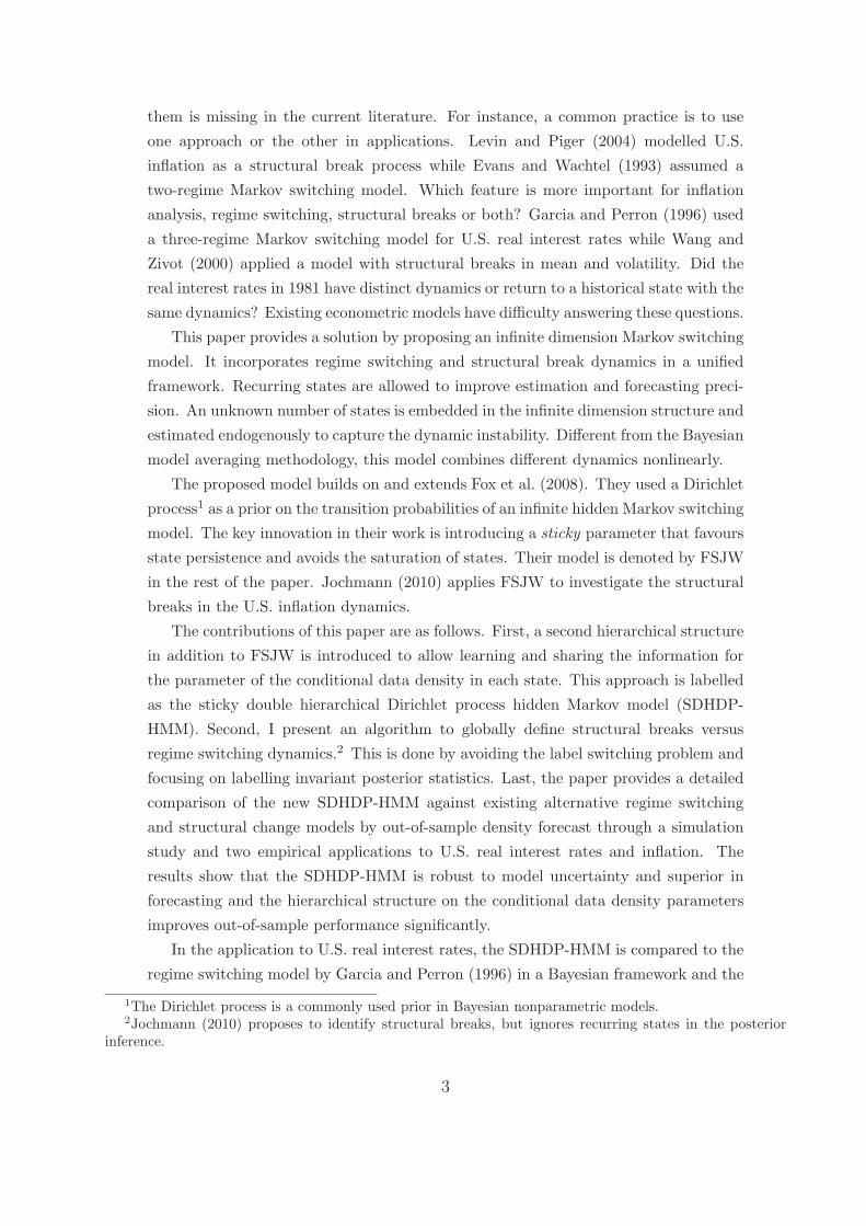
Figure 1: The horizontal dimension from left to right represents time and thevertical circles represent different states. The numbers in the circles are thelabels of the states and they are exchangeable. The SDHDP-HMM nests: (a) nostate change, (b) regime switching, (c) structural breaks, (d) frequent parameterchange and (e) regime switching and structural breaks.

32

time

12

34

structural breakregime switching

Figure 2: Example of the global identification of regime switching and structuralbreaks. All the points represent one sample of the states (s1, · · · , sT ) from the posteriorsamples. The circles are non-recurrent states which only appear for one consecutiveperiod and the triangles are recurrent states. The solid arrows point to the breakpoints and the dashed arrows point to the switching points.

33

0 200 400 600 800 1000

−15

−10

−5

05

10

time

Figure 3: Data simulated by a SDHDP-HMM. Each state has Gaussian AR(2) dynam-ics: yt = φst0 + φst1yt−1 + φst2yt−2 + σst

εt.

34

−1.

0−

0.5

0.0

0.5

1.0

Time

Inte

rcep

t

TrueEstimated

50 150 250 350 450 550 650 750 850 950

−1.

0−

0.5

0.0

0.5

1.0

Time

Per

sist

ence

TrueEstimated

50 150 250 350 450 550 650 750 850 950

12

34

56

Time

Std True

Estimated

50 150 250 350 450 550 650 750 850 950

12

34

56

Time

num

ber

of s

tate

s

TrueEstimated

50 150 250 350 450 550 650 750 850 950

Figure 4: The SDHDP-HMM estimates the data in figure 3. Each state has GaussianAR(2) dynamics: yt = φst0 + φst1yt−1 + φst2yt−2 + σst

εt. The solid lines are the truevalues and the dashed lines are the posterior means of those values estimated by theSDHDP-HMM. The top-left panel plots the intercepts φst0; the top-right panel plotsthe persistence parameters φst1 + φst2; the bottom-left plots the conditional standarddeviations σst

and the bottom-right plots the cumulative number of the active states(active state means it has been visited at least once).

35

0 200 400 600 800 1000

−4

−2

02

46

8

time

Figure 5: Data simulated by a 3-state Markov switching model of (27)-(30). Each statehas Gaussian AR(2) dynamics: yt = φst0 + φst1yt−1 + φst2yt−2 + σst

εt.

36

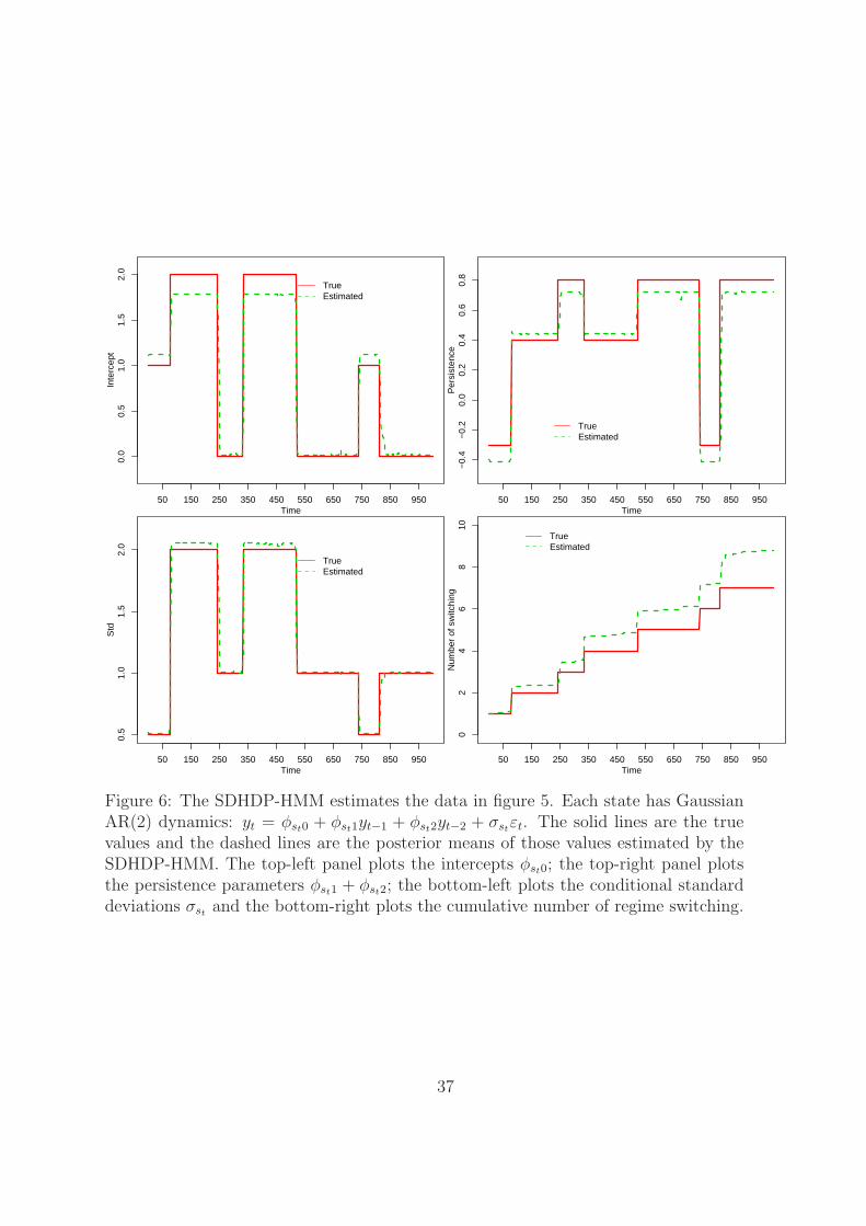
0.0

0.5

1.0

1.5

2.0

Time

Inte

rcep

t

TrueEstimated

50 150 250 350 450 550 650 750 850 950

−0.

4−

0.2

0.0

0.2

0.4

0.6

0.8

Time

Per

sist

ence

TrueEstimated

50 150 250 350 450 550 650 750 850 950

0.5

1.0

1.5

2.0

Time

Std

TrueEstimated

50 150 250 350 450 550 650 750 850 950

02

46

810

Time

Num

ber

of s

witc

hing

TrueEstimated

50 150 250 350 450 550 650 750 850 950

Figure 6: The SDHDP-HMM estimates the data in figure 5. Each state has GaussianAR(2) dynamics: yt = φst0 + φst1yt−1 + φst2yt−2 + σst

εt. The solid lines are the truevalues and the dashed lines are the posterior means of those values estimated by theSDHDP-HMM. The top-left panel plots the intercepts φst0; the top-right panel plotsthe persistence parameters φst1 + φst2; the bottom-left plots the conditional standarddeviations σst

and the bottom-right plots the cumulative number of regime switching.

37

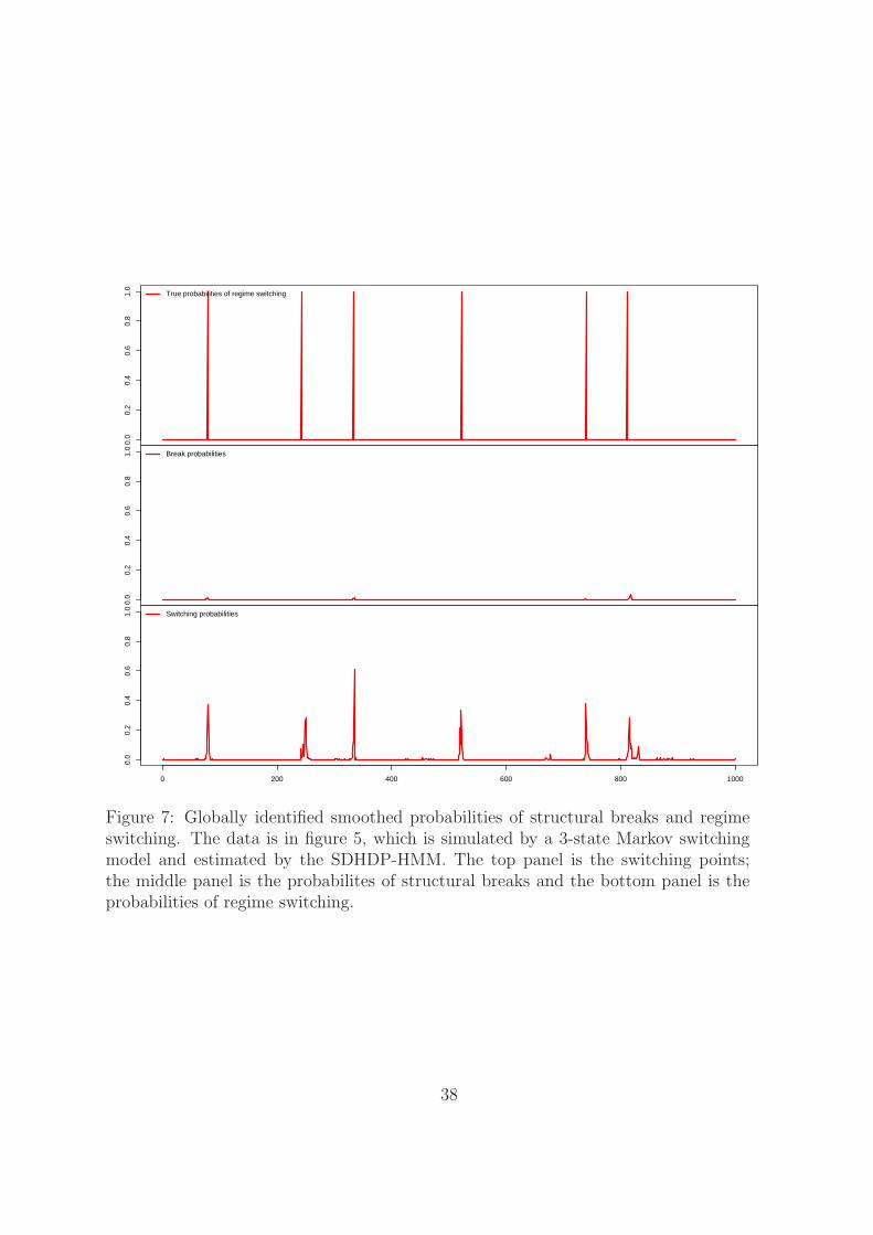
0.0

0.2

0.4

0.6

0.8

1.0

True probabilities of regime switching

0.0

0.2

0.4

0.6

0.8

1.0

Break probabilities

0 200 400 600 800 1000

0.0

0.2

0.4

0.6

0.8

1.0

Switching probabilities

Figure 7: Globally identified smoothed probabilities of structural breaks and regimeswitching. The data is in figure 5, which is simulated by a 3-state Markov switchingmodel and estimated by the SDHDP-HMM. The top panel is the switching points;the middle panel is the probabilites of structural breaks and the bottom panel is theprobabilities of regime switching.

38

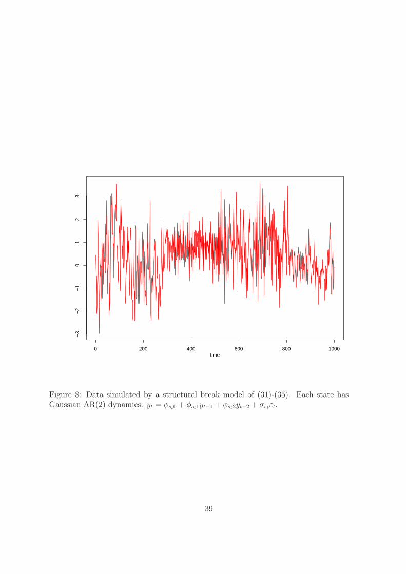
0 200 400 600 800 1000

−3

−2

−1

01

23

time

Figure 8: Data simulated by a structural break model of (31)-(35). Each state hasGaussian AR(2) dynamics: yt = φst0 + φst1yt−1 + φst2yt−2 + σst

εt.

39

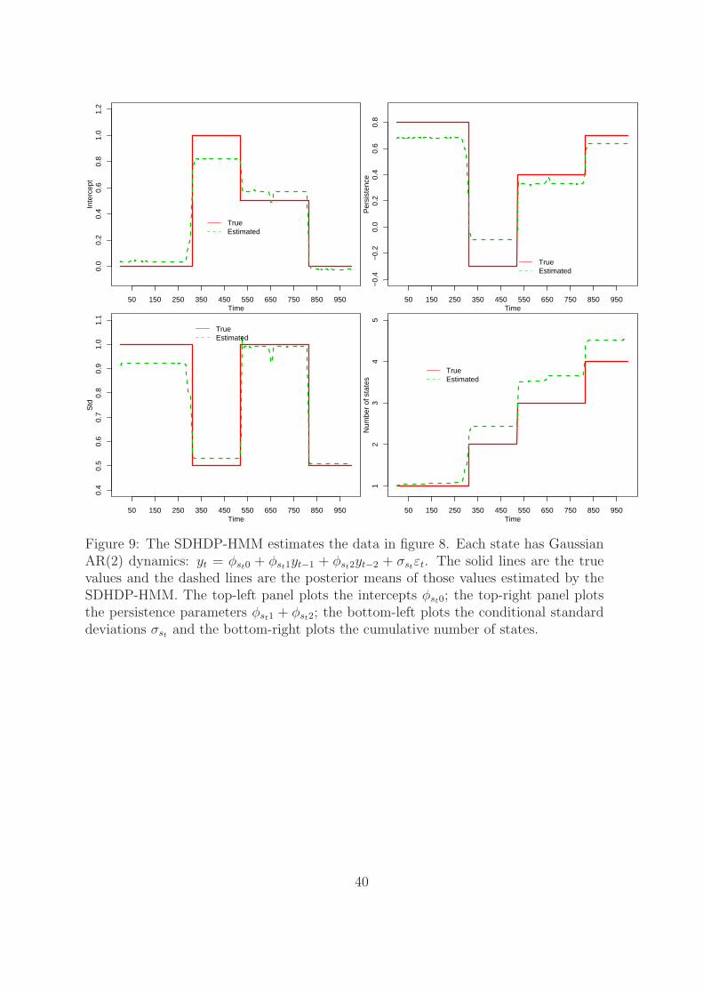
0.0

0.2

0.4

0.6

0.8

1.0

1.2

Time

Inte

rcep

t

TrueEstimated

50 150 250 350 450 550 650 750 850 950

−0.

4−

0.2

0.0

0.2

0.4

0.6

0.8

Time

Per

sist

ence

TrueEstimated

50 150 250 350 450 550 650 750 850 950

0.4

0.5

0.6

0.7

0.8

0.9

1.0

1.1

Time

Std

TrueEstimated

50 150 250 350 450 550 650 750 850 950

12

34

5

Time

Num

ber

of s

tate

sTrueEstimated

50 150 250 350 450 550 650 750 850 950

Figure 9: The SDHDP-HMM estimates the data in figure 8. Each state has GaussianAR(2) dynamics: yt = φst0 + φst1yt−1 + φst2yt−2 + σst

εt. The solid lines are the truevalues and the dashed lines are the posterior means of those values estimated by theSDHDP-HMM. The top-left panel plots the intercepts φst0; the top-right panel plotsthe persistence parameters φst1 + φst2; the bottom-left plots the conditional standarddeviations σst

and the bottom-right plots the cumulative number of states.

40

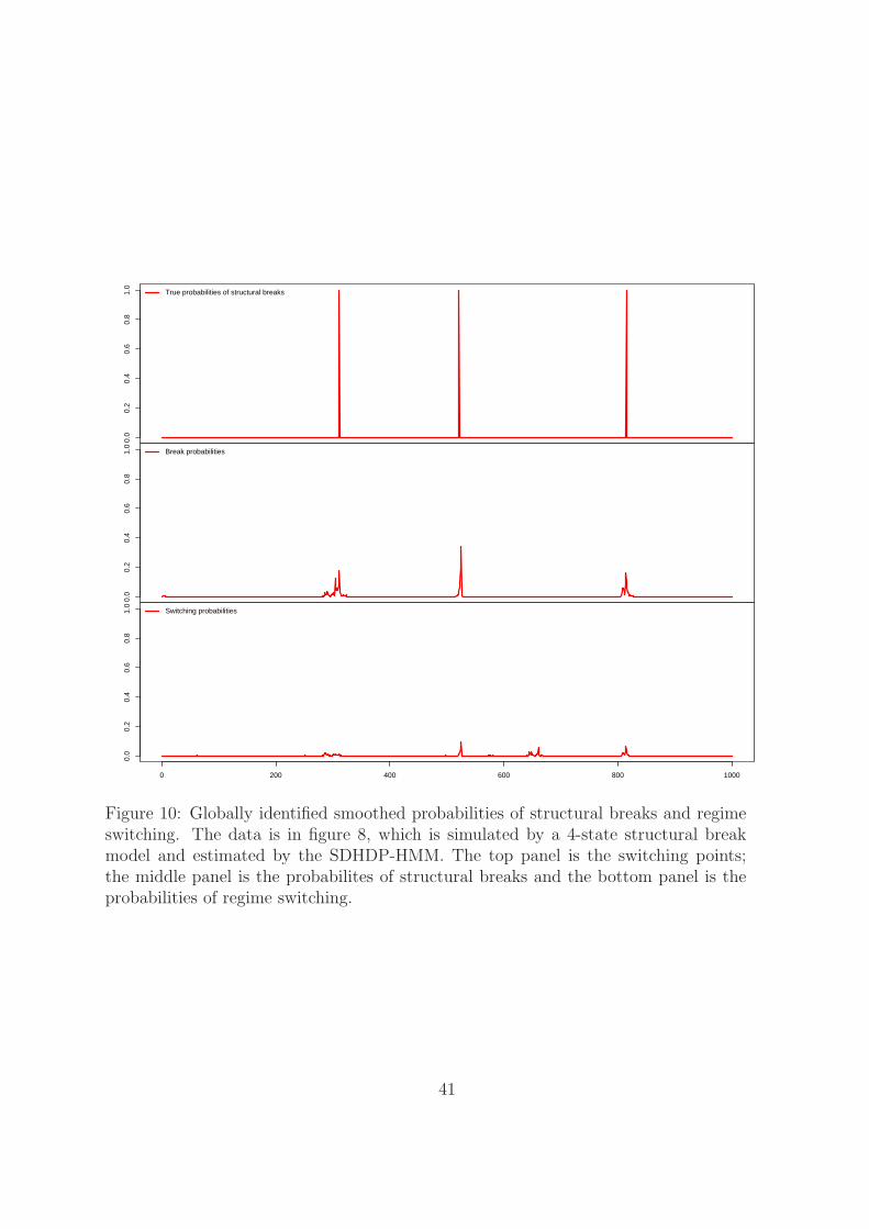
0.0

0.2

0.4

0.6

0.8

1.0

True probabilities of structural breaks

0.0

0.2

0.4

0.6

0.8

1.0

Break probabilities

0 200 400 600 800 1000

0.0

0.2

0.4

0.6

0.8

1.0

Switching probabilities

Figure 10: Globally identified smoothed probabilities of structural breaks and regimeswitching. The data is in figure 8, which is simulated by a 4-state structural breakmodel and estimated by the SDHDP-HMM. The top panel is the switching points;the middle panel is the probabilites of structural breaks and the bottom panel is theprobabilities of regime switching.

41

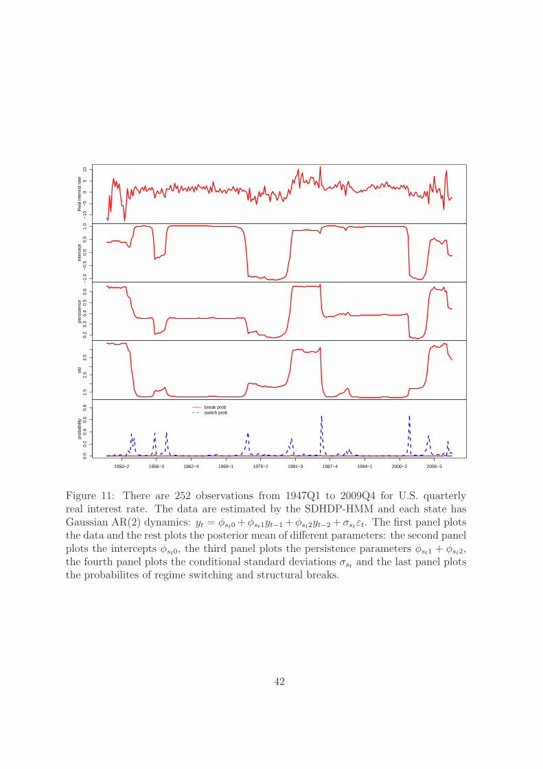
−10

−5

05

10R

eal i

nter

est r

ate

−1.

0−

0.5

0.0

0.5

1.0

inte

rcep

t0.

20.

30.

40.

50.

6pe

rsis

tenc

e1.

52.

53.

5st

d0.

00.

20.

40.

60.

8pr

obab

ility

break probswitch prob

1950−2 1956−3 1962−4 1969−1 1975−2 1981−3 1987−4 1994−1 2000−2 2006−3

Figure 11: There are 252 observations from 1947Q1 to 2009Q4 for U.S. quarterlyreal interest rate. The data are estimated by the SDHDP-HMM and each state hasGaussian AR(2) dynamics: yt = φst0 + φst1yt−1 + φst2yt−2 + σst

εt. The first panel plotsthe data and the rest plots the posterior mean of different parameters: the second panelplots the intercepts φst0, the third panel plots the persistence parameters φst1 + φst2,the fourth panel plots the conditional standard deviations σst

and the last panel plotsthe probabilites of regime switching and structural breaks.

42

Figure 12: There are 252 observations from 1947Q1 to 2009Q4 for U.S. quarterlyreal interest rate. The data are estimated by the SDHDP-HMM and each state hasGaussian AR(2) dynamics: yt = φst0 + φst1yt−1 + φst2yt−2 + σst

εt. The top panel plotsthe data and the bottom panel plots the posterior mean of the cumulative number ofactive states (active state means it has been visited at least once).

43

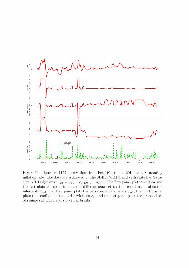
−10

010

20In

flatio

n−

3−

10

12

3in

terc

ept

0.85

0.90

0.95

1.00

pers

iste

nce

0.5

1.0

1.5

std

0.0

0.2

0.4

0.6

0.8

prob

abili

ty

break probswitch prob

191810 192805 193801 194708 195703 196610 197605 198601 199508 200503

Figure 13: There are 1153 observations from Feb 1914 to Jan 2010 for U.S. monthlyinflation rate. The data are estimated by the SDHDP-HMM and each state has Gaus-sian AR(1) dynamics: yt = φst0 + φst1yt−1 + σst

εt. The first panel plots the data andthe rest plots the posterior mean of different parameters: the second panel plots theintercepts φst0, the third panel plots the persistence parameters φst1, the fourth panelplots the conditional standard deviations σst

and the last panel plots the probabilitesof regime switching and structural breaks.

44

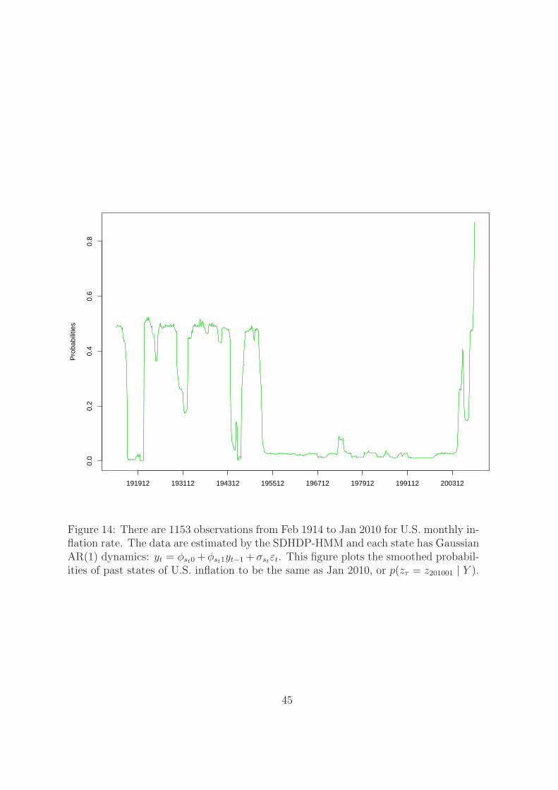
0.0

0.2

0.4

0.6

0.8

Pro

babi

litie

s

191912 193112 194312 195512 196712 197912 199112 200312

Figure 14: There are 1153 observations from Feb 1914 to Jan 2010 for U.S. monthly in-flation rate. The data are estimated by the SDHDP-HMM and each state has GaussianAR(1) dynamics: yt = φst0 + φst1yt−1 + σst

εt. This figure plots the smoothed probabil-ities of past states of U.S. inflation to be the same as Jan 2010, or p(zτ = z201001 | Y ).

45

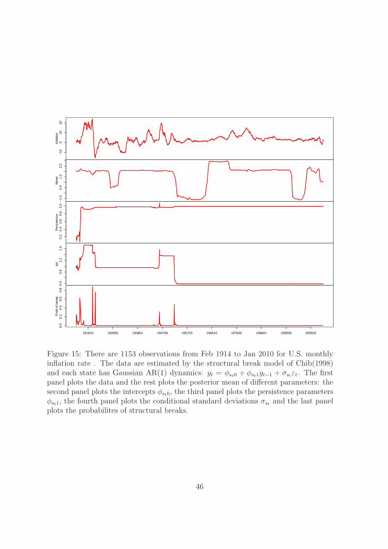
−10

010

20In

flatio

n−

1.0

0.0

1.0

2.0

Mea

n0.

20.

40.

60.

81.

0P

ersi

sten

ce0.

40.

81.

21.

6st

d0.

00.

20.

40.

60.

8P

rob

of b

reak

191810 192805 193801 194708 195703 196610 197605 198601 199508 200503

Figure 15: There are 1153 observations from Feb 1914 to Jan 2010 for U.S. monthlyinflation rate . The data are estimated by the structural break model of Chib(1998)and each state has Gaussian AR(1) dynamics: yt = φst0 + φst1yt−1 + σst

εt. The firstpanel plots the data and the rest plots the posterior mean of different parameters: thesecond panel plots the intercepts φst0, the third panel plots the persistence parametersφst1, the fourth panel plots the conditional standard deviations σst

and the last panelplots the probabilites of structural breaks.

46

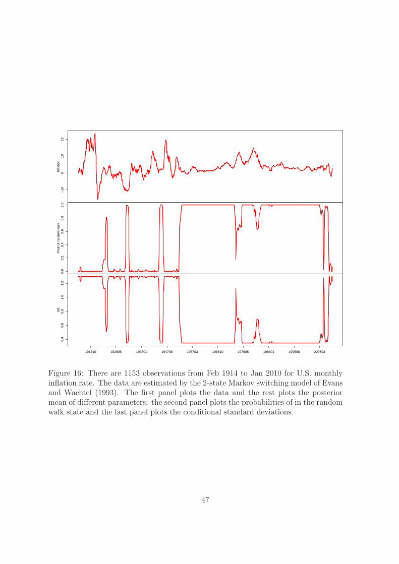
−10

010

20In

flatio

n0.

00.

20.

40.

60.

81.

0P

rob

of r

ando

m w

alk

0.4

0.6

0.8

1.0

1.2

std

191810 192805 193801 194708 195703 196610 197605 198601 199508 200503

Figure 16: There are 1153 observations from Feb 1914 to Jan 2010 for U.S. monthlyinflation rate. The data are estimated by the 2-state Markov switching model of Evansand Wachtel (1993). The first panel plots the data and the rest plots the posteriormean of different parameters: the second panel plots the probabilities of in the randomwalk state and the last panel plots the conditional standard deviations.

47

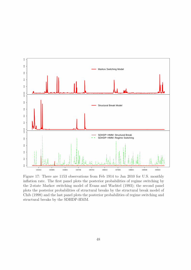
0.0

0.2

0.4

0.6

0.8

1.0

Markov Switching Model

0.0

0.2

0.4

0.6

0.8

1.0

Structural Break Model

0.0

0.2

0.4

0.6

0.8

1.0

SDHDP−HMM: Structural BreakSDHDP−HMM: Regime Switching

191810 192805 193801 194708 195703 196610 197605 198601 199508 200503

Figure 17: There are 1153 observations from Feb 1914 to Jan 2010 for U.S. monthlyinflation rate. The first panel plots the posterior probabilities of regime switching bythe 2-state Markov switching model of Evans and Wachtel (1993); the second panelplots the posterior probabilities of structural breaks by the structural break model ofChib (1998) and the last panel plots the posterior probabilities of regime switching andstructural breaks by the SDHDP-HMM.

48