structural breaks in the game: the case of major league

Structural Breaks in the Game: The Case of Major League Baseball

Peter A. Groothuis

Walker College of Business

Appalachian State University

Boone, NC 28608

Kurt W. Rotthoff

Stillman School of Business

Seton Hall University

South Orange, NJ 07079

Mark C. Strazicich

Department of Economics

Appalachian State University

Boone, NC 28608

March 12, 2015

Abstract: To search for eras in a sports league, we utilize time series tests with structural

breaks to identify eras in Major League Baseball performance. Using data from 1871-

2010, the mean and standard deviation of four different performance measures are

examined to test if deterministic or stochastic trends and structural breaks are present.

Throughout, we identify breaks endogenously from the data. Perhaps most notable

among our findings, we identify a deterministic trend in the mean slugging percentage in

1921 and 1992, which coincides with the early years of the free swinging (Babe Ruth) era

and the modern steroid era, respectively.

JEL Classifications: J24, Z2, C22

Keywords: Major League Baseball, Technological Change, Structural Breaks

1

1. Introduction

Over time, games change and new innovations are developed. In many sports the

equipment drives these changes; such as innovations in tennis rackets, golf club

technologies, or swim suits (now banned). In other sports change might result from the

development of a new defensive technique (Lawrence Taylor), a new way to swing the

bat (Babe Ruth), throw a pitch ("Bullet Joe" Bush), shoot a basket (Goose Tatum), or

hold a putter (the current debate over the belly-putter). As players adopt successful

innovations they are mimicked and the game can change.

Sports historians and scholars have often assumed exogenous changes in the game

based on particular historical events. For instance, in baseball, one historian suggests that

the game changed in 1920 when Ray Chapman was killed by a pitch that year and

baseball responded by banning the spitball (Okrent, 1989). In contrast, we make no prior

judgments about the timing of eras. Instead, we let the data speak to endogenously

identify eras. To do so, we utilize time series tests with structural breaks to identify eras.

Utilizing time series tests to analyze sports data has only recently become more popular

in the literature and is most prominent in the works of Fort and Lee (2006, 2007), Lee

and Fort (2005, 2008, 2012), and Mills and Fort (2014), who employ unit root and

structural break tests to examine competitive balance in a number of sports.1 In the

present paper, we adopt a similar methodological approach and examine time series on

the mean and standard deviation of four traditional Major League Baseball (MLB)

performance measures. Our goal is to identify the timing of eras in MLB performance

that may not have been apparent when focusing a priori on particular historical events.

1 See also the works of Scully (1995), Palacios-Huerta (2004), Schmidt and Berri (2004), and Nieswiadomy et al. (2012).

2

We find that most MLB performance measures are stationary around a

deterministic trend with one or more structural breaks. Perhaps most notable among our

findings, we identify a deterministic trend in the mean slugging percentage that shifts

upward and changes slope in 1921 and 1992, which corresponds with the early years of

the free swinging (Babe Ruth) era and the modern steroid era, respectively. We conclude

that structural breaks should be considered when identifying eras and comparing

performance over time. The paper proceeds as follows. The data and testing procedures

are described in Section 2 and results in Section 3. We conclude in Section 4.

2. Data and Structural Breaks

MLB attracts the best baseball players in the world. The first professional baseball

team was established in 1869 (the “Cincinnati Red Stockings”) and the league itself

started in the late 1800s (and continues today). The best players in the league have their

names written in the record books. However, changes in the game have led to questions

about how records should be kept. For example, Barry Bonds has the most homeruns in

one season, 73 in 2001, while Babe Ruth hit 60 home runs in 1927. However, there were

162 games a season in 2001, but only 154 games in 1927 and some rules differed. While

the number of homeruns per game is higher for Barry Bonds, differences in the game due

to different technologies, rules, and style of play can matter.

Using data from Sean Lahman’s Baseball Database on all MLB players from

1871-2010 with at least 100 at-bats, we measure slugging percentage (SLUG), home runs

per hundred at bats (HR), batting average (BAVE), and runs batted in per hundred at bats

(RBI).2 With 35,728 single season observations we find that the average player hit 7

2 Sean Lahman’s Baseball Database: http://baseball1.com/2011/01/baseball-database-updated-

2010/. Slugging percentage is calculated as total bases divided by the number of at-bats.

3

homeruns per season (with a maximum of 73), had 42.5 runs batted in (RBI), and a

slugging percentage of .379. Using the data for each player, we calculate both the mean

and standard deviation of each performance measure for each season. This provides

annual time series from 1871-2010 that consist of 140 seasonal observations for each

series. We utilize these eight time series in our empirical investigation. A summary of the

mean and standard deviation of our data is provided in Table 1.3

To determine if the time series measures of player performance are stationary

around a deterministic trend or non-stationary (stochastic trend) and to look for structural

breaks, we begin by utilizing the two-break minimum LM unit root test proposed by Lee

and Strazicich (2003).4 To endogenously identify the location of two breaks (j = TBj/T,

j=1, 2), the minimum LM unit root test uses a grid search to determine the combination

of breaks where the unit root test statistic is minimized (i.e., the most negative). Since

critical values for the model with trend-break vary (somewhat) depending on the location

of the breaks (j), we employ critical values corresponding to the identified break points.

Serial correlation is corrected by including lagged first-differenced terms selected by a

sequential “general to specific” procedure.5 The process is repeated for each combination

3 We use only hitting statistics because of the length of the time series and because preliminary

analysis on pitching statistics provided no structural breaks. 4 By “structural break,” we imply a significant, but infrequent, permanent change in the level

and/or trend of a time series. See Enders (2010) for additional background discussion on

structural breaks and unit root tests. 5 To determine the number of lagged first-differenced terms that correct for serial correlation, we

employ the following sequential “general to specific” procedure. At each combination of two

break points over the time interval [.1T, .9T] (to eliminate end points) we begin with a maximum

number of k = 8 lagged first-difference terms and examine the last term to see if its t-statistic is significantly different from zero at the 10% level (critical value of 1.645 in an asymptotic normal

distribution). If insignificant, the k = 8 term is dropped and the model is re-estimated using k = 7

terms, etc., until the maximum lagged term is found (i.e., the order of serial correlation is

identified and corrected), or k = 0 (i.e., there is no serial correlation). Once the maximum number of lagged terms is found, all lower lags remain in the unit root test. This type of procedure has

4

of two breaks to jointly identify the breaks and unit root test statistic where the unit root

test statistic is minimized.6 In each case, we begin by applying the two-break LM unit

root test. If only one break is identified (at the 10% level of significance), we re-examine

the series using the one-break LM unit root test (Lee and Strazicich, 2013). If no break is

identified, we then utilize the conventional (no-break) augmented Dickey-Fuller unit test

(Dickey and Fuller, 1979, 1981). Rejection of the null indicates that the series is

stationary around a deterministic trend. In contrast, failure to reject the null implies a

nonstationary series with a stochastic trend. 7

After identifying the time series that are stationary around one or two breaks, we

next perform tests to see if additional breaks are present. To do so, we utilize the multiple

break tests suggested by Bai and Perron (1998, 2003, BP hereafter). Given that the BP

tests are valid only for stationary time series, we begin by performing regressions on the

level and trend breaks for the series identified as stationary with two breaks.8 We then

apply the BP test to the residuals of these regressions to search for additional breaks.

Given that the breaks in these regressions are the same as those that reject the unit root

hypothesis in the two-break LM unit root test, the residuals of these regressions will be

stationary and the BP test can be safely applied to search for additional breaks.9

been shown to perform well compared to other data-dependent procedures to select the optimal k and correct for serial correlation (e.g., Ng and Perron, 1995). 6 Gauss codes for the one- and two-break minimum LM unit root test are available from the

authors upon request. 7 Note that the interpretation of breaks in a nonstationary (unit root) series differs from that in a

stationary series. In a unit root process, a structural break in the level can be interpreted as an

unusually large one-time shock or outlier, while a break in the trend can be interpreted as a permanent change in the drift. 8 See Prodan (2008) for a discussion of pitfalls that can arise when applying the Bai and Perron

(1998, 2003) type tests to nonstationary time series. 9 See Lee and Fort (2005, 2008, 2012), Fort and Lee (2006, 2007), Bai and Perron (1998, 2003),

and Lee and Strazicich (2003, 2013) for more detailed discussion of the tests described above.

5

3. Results

We begin by discussing the LM unit root test results displayed in Table 2. The

slugging percentage mean (SLUGM) rejects the unit root null hypothesis at the 5%

significance level in the two-break test, implying that SLUGM is a stationary series with

structural breaks in 1921 and 1992. For the slugging percentage standard deviation

(SLUGSD), only one break was significant in the two-break test. We therefore re-tested

this series using the one-break test. In contrast to SLUGM, the SLUGSD cannot reject a

unit root at the 10% level of significance, indicating that this series is nonstationary and

has a stochastic trend. Similarly, the unit root hypothesis cannot be rejected for the

homerun mean (HRM) at the 10% level of significance, implying that this series is

nonstationary. In contrast, the unit root hypothesis is rejected for the homerun standard

deviation (HRSD) at the 5% level of significance, indicating that this series is stationary

with structural breaks in 1920 and 1966. The batting average mean (BAVEM) cannot

reject the unit root hypothesis at the 10% level of significance, implying that BAVEM is

a nonstationary series. In contrast, the batting average standard deviation (BAVESD)

rejects the unit root hypothesis at the 1% level of significance, implying that BAVESD is

a stationary series with breaks in 1906 and 1933. The runs batted in mean (RBIM) rejects

the unit root hypothesis at the 10% level of significance, implying that RBIM is a

stationary series with a break in 1887. The runs batted in standard deviation (RBISD)

rejects the unit root hypothesis at the 5% level of significance, implying that RBISD is a

stationary series with a break in 1921.

We next perform regressions on the level and trend breaks for the five

performance measures that reject the unit root hypothesis in Table 2 (SLUGM, HRSD,

6

BAVESD, RBIM, and RBISD).10

The results are displayed in Table 3. White’s robust

standard errors are used to control for heteroskedasticity. Serial correlation is corrected

by including lagged values of the dependent variable identified by a similar general to

specific procedure as described in footnote 5.11

In each case, Ljung-Box Q-statistics for

24 lags indicate that the null hypothesis of no remaining serial correlations cannot be

rejected at the 10% level of significance. Using the residuals from the regressions with

two breaks in Table 3, we then apply the multiple break BP test to SLUGM, HRSD, and

BAVESD to search for additional breaks. A summary of the identified breaks is

displayed in Table 4. Compared to the two breaks identified by the LM unit root test for

SLUGM, HRSD, and BAVESD, the BP tests finds two additional breaks for each of

these series. For SLUGM, the BP tests finds additional breaks in 1902 and 1920. Given

that the break in 1920 is nearly identical to the break in 1921 identified by the LM unit

root test, we will ignore this additional break in the discussion that follows. For HRSD,

the BP test finds additional breaks in 1940 and 1945 during the period of World War II.

For BAVESD, the BP tests finds additional breaks in 1879 and 1883.

To more carefully examine the sign and significance of including the additional

breaks, we next perform regressions for the three series containing more than two breaks

in Table 4 (i.e., SLUGM, HRSD, and BAVESD). Robust standard errors and lagged

dependent variables are again included in each regression to control for

heteroskedasticity and serial correlation. The results are reported in Table 5.12

We begin

10

Regressions will not be undertaken for SLUGSD, HRM, and BAVEM, since these series are nonstationary and spurious regressions can occur. 11

See Ashley (2012) for discussion of why modeling serial correlation in regressions with lagged

variables is a desirable procedure. 12

As in Table 3, in each case the Ljung-Box Q-statistics for 24 lags indicate that the null hypothesis of no remaining serial correlations cannot be rejected at the 10% level of significance.

7

by discussing results for the slugging percentage mean (SLUGM). There is a downward

shift in SLUGM in 1902, the additional break identified by the BP test, while the break

coefficient is not statistically significant. Following this, there is a significant upward

shift in the mean slugging percentage in 1921 and another upward shift in 1992. The

break in 1921 coincides with the early years of the free swinging (Babe Ruth) era while

1992 coincides with the early years of the modern steroid era often associated with Jose

Canseco and Mark McGwire, among others.13

Following the upward shift in 1992, there

is a small but significant downward trend in SLUGM.

We next examine regression results for the standard deviation of home runs

(HRSD). Following the break in 1920, there is a significant upward shift in HRSD

indicating that the dispersion in home run performance increased. Following this, there is

a significant downward shift in 1940 followed by a significant upward shift in 1945.

After the final break in 1966, there a significant downward shift in HRSD with a small

but significant upward trend. Perhaps most notable among these findings is that we again

see a significant structural break in 1920 associated with the early years of the free

swinging (Babe Ruth) era. These findings provide additional support to the idea that the

Babe Ruth era had a major influence on the game. During this time there were two major

events: Babe Ruth influenced the game by creating a batting style that could be, and was,

emulated by other players. Moreover, at the same time, the type of ball and style of

pitching changed. We suggest that combined these changes had a significant impact on

the game, which lead to a greater dispersion in home run performance among players.

13

For example, in a statement released on the web site of the St. Louis Cardinals on January 11, 2010, Mark McGwire admitted using performance enhancing drugs beginning in 1989 or 1990.

8

We next examine the regression results for the batting average standard deviation

(BAVESD). Following the break in 1879, there is a significant (at the 10% level)

downward shift in BAVESD followed soon after by a significant upward shift in 1883.

Following this there is a significant upward shift in 1906 and significant downward shift

in 1933. After the final break in 1933, there is slight but significant downward trend in

BAVESD.

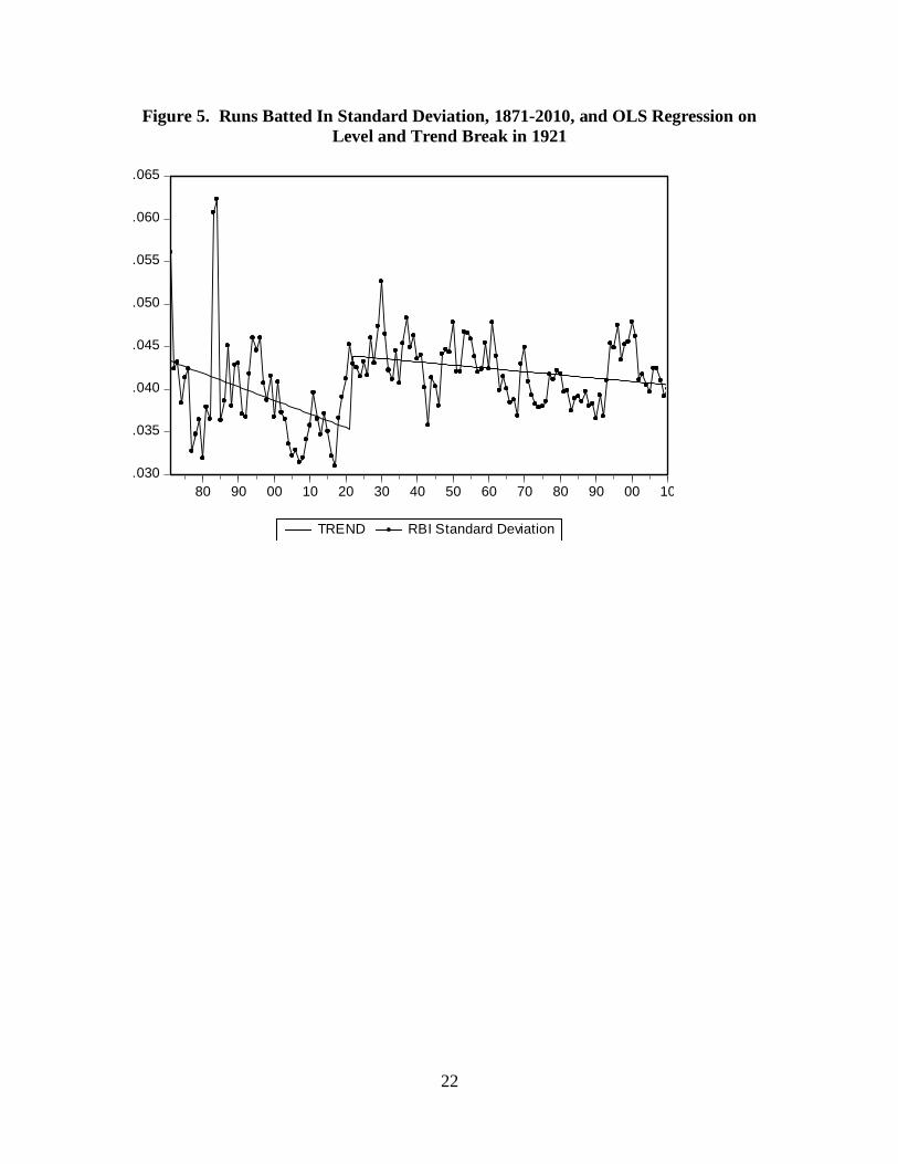
Next, we examine results for the mean and standard deviation of runs batted in

(RBIM and RBISD) using the single break regression results in Table 3. Following the

break in 1887 there is an upward shift in RBIM. While there is a slight positive trend

following the break, the trend slope is not significant (at the 10% level). For RBISD,

following the break in 1921 there is an upward shift in RBISD. There is a slight negative

trend following the break, but the trend slope is not significant (at the 10% level). While

the break in RBISD is again associated with the Babe Ruth era, there is little notable

change in the series before and after the break. Overall, the results for RBI suggest that

there has been little change in RBIM and RBISD.

To better visualize the regression results of the stationary series with breaks

reported in Table 5 (SLUGM, HRSD, and BAVESD) and Table 3 (RBIM and RBISD),

we next construct simple plots of the estimated trends and actual data in Figures 1-5. As

in the regression results described above, perhaps most interesting is the plot of the

slugging percentage mean (SLUGM) displayed in Figure 1. From Figure 1, we can easily

observe the significant upward shifts in SLUGM that occurred in 1921 and 1992, with the

biggest upward shift apparent in 1921 during the early years of the Babe Ruth era.

Similarly, in Figure 2, we see a notable upward shift in the standard deviation of home

9

runs (HRSD) in 1920. In Figure 3, we can observe the general decline in the batting

average standard deviation (BAVESD). In Figures 4 and 5, we observe the relative

stability of the mean and standard deviation of runs batted in (RBIM and RBISD),

respectively.

The above results suggest that MLB performance had a notable structural break

around 1920-1921. The trend in the slugging percentage mean (SLUGM) had a positive

upward shift in 1921 suggesting that the average player began to increasingly hit for

power and hit more doubles, triples, and home runs. Similarly, the trend in the home run

standard deviation (HRSD) had an upward shift and increasing slope in 1920 and the runs

batted in standard deviation (RBISD) had a positive (small) upward shift in 1921. These

findings suggest that players after 1920 became more diverse in their performance with

some players increasingly hitting for power while others did not. Combined with the

1921 break in the slugging percentage mean (SLUGM), these findings suggest the

possibility that following the success of Babe Ruth’s free swinging style, combined with

the required pitching changes that occurred at this time, others that could mimicked his

innovation and hit for power as well.

It is interesting to note that our endogenous stuctural break in 1921 occurs close to

a historical break often identified by baseball historians. To provide historal context to

this era Rothman (2012), a baseball historian, suggests that the 1920’s changed the

offensive strategies in baseball due to three major events: The Black Sox scandal, the

banning of the spitball, and Babe Ruth’s style of hitting being copied. The Black Sox

scandal occurred in 1919 and caused the popularity of baseball to decline. Rothman

further suggests that in an attempt to clean up the Black Sox scandal of 1919, the spitball

10

and other trick pitches were abolished starting in 1920 (which also came after the death

of Ray Chapman in 1920, for which “umpires were ordered to only use shiny white balls

throughout the game”). Rothman further suggests that in 1919, when Babe Ruth hit a

record 29 home runs during his last year with the Red Sox, that this created a notable

increase in fan excitement about home runs. These events coincide with our suggestion

that starting in 1920 and 1921 many players increasingly copied Babe Ruth’s hitting

style. This style included not choking up on the bat and swinging with a pronounced

upper-cut. Ruth’s style replaced the spray-hitting style that resulted in many singles.

Rothman also notes that attendance in 1920 increased approximately 20% from 1919. As

owners noticed this increase in attendance, they attribited this to an increase in offensive

performance and home run hitting, which encouraged an increased adoption of this new

style of hitting. We suggest that the structural break that we identify in 1921 is consistent

with all three of the events described above; during, what most people remember as, the

“Babe Ruth era.”

Most notable among our other breaks is the significant upward shift in the

slugging perecentage mean (SLUGM) found in 1992, which is closely associated with

(what many preceive to be) the early years of the modern steriod era. Although it is

difficult to identify the start of the steriod era since players attempt to keep hidden the use

of performance enhancing drugs, it is interesting to note that while MLB banned steriods

in 1991 they did not test for their useage until 2003. We suggest that fan interest in

offensive performance (Ahn and Lee, 2014), coupled with the the knowledge that steriods

were becoming an issue in MLB due to the explicit ban, might have caused the structrual

break in 1992 as players mimicked steriod use knowing they would not be caught.

11

4. Conclusion

Over time, games change. Most analysts identify exogenous changes in the game

based on particular historical events. In contrast, we utilize time series techniques to

endogenously determine where changes occur. Using several time series on Major

League Baseball performance from 1871-2010 (140 seasonal observations for each

series), we attempt to determine if structural breaks can be used to define different eras.

Using several measures of batting performance, we perform time series tests to

identify if deterministic or stochastic trends and structural breaks are present. Perhaps

most notable among our findings, we identify significant structural breaks in 1921 and

1992 for the mean slugging percentage. Given that the breaks are endogenously

determined from the data, it is interesting to analyze what was happening in the sport

during these years.

Interestingly, the break in 1921 coincides with the early years of the free swinging

era often identified with Babe Ruth. We suggest that during this time, other players began

to mimic Babe Ruth’s free-swinging style. In addition, pitching rules changed at this

time. Combined, we suggest that these events had a major influence on baseball and

changed the game. Finally, our identified structural break in 1992 is consistent with

historical observations commonly associated with the early years of the modern steroid

era. In particular, it is interesting to note that 1992 is one year after Major League

Baseball enacted a ban on steroid use while the ban was not enforced with testing until

2003. In conclusion, we suggest that the findings presented here support utilizing time

series tests with structural breaks to identify eras in sports and provide insights for future

research.

12

References

Ahn, Seung C., and Lee, Young H. (2014). “Major League Baseball Attendance: Long-

Term Analysis Using Factor Models,” Journal of Sports Economics 15(5), 451-477.

Ashley, Richard A. (2012). Fundamentals of Applied Econometrics, Hoboken, NJ: John

Wiley & Sons, Inc.

Bai, J. and P. Perron (1998). “Estimating and Testing Linear Models with Multiple

Structural Changes,” Econometrica 66, 47-78.

Bai, J. and P. Perron (2003). “Computation and Analysis of Multiple Structural Change

Models,” Journal of Applied Econometrics 18, 1-22.

Dickey, David A. and Wayne A. Fuller (1979). “Distribution of the Estimator for

Autoregressive Time Series with a Unit Root,” Journal of the American Statistical

Association 74 (366), 427-431.

Dickey, David A. and Wayne A. Fuller (1981). “Likelihood Ratio Statistics for

Autoregressive Time Series with a Unit Root.” Econometrica 49, 1057-1072.

Enders, Walter (2010). Applied Econometric Time Series, 3rd

edition. Hoboken, NJ: John

Wiley & Sons, Inc.

Fort, Rodney and Young Hoon Lee (2006). “Stationarity and Major League Baseball

Attendance Analysis,” Journal of Sports Economics 7(4), 408–415.

Fort, Rodney and Young Hoon Lee (2007). “Structural Change, Competitive Balance,

and the Rest of the Major Leagues,” Economic Inquiry 45(3), 519-532.

Lee, Young Hoon, and Rodney Fort (2005). “Structural Change in Baseball’s

Competitive Balance: The Great Depression, Team Location, and Racial

Integration,” Economic Inquiry 43, 158-169.

13

Lee, Young Hoon, and Rodney Fort (2008). “Attendance and the Uncertainty-of-

Outcome Hypothesis in Baseball,” Review of Industrial Organization 33, 281-295.

Lee, Young Hoon, and Rodney Fort (2012). “Competitive Balance: Time Series Lessons

from the English Premier League,” Scottish Journal of Political Economy 59(3),

266-282.

Lee, J., and M. C. Strazicich (2003). “Minimum Lagrange Multiplier Unit Root Test with

Two Structural Breaks,” Review of Economics and Statistics 8(4), 1082-1089.

Lee, J., and M. C. Strazicich (2013). “Minimum LM Unit Root Test with One Structural

Break,” Economics Bulletin 33(4), 2483-2492.

Mills, Brian, and Rodney Fort (2014). “League-Level Attendance and Outcome

Uncertainty in U.S. Pro Sports Leagues,” Economic Inquiry 52(1), 205-218.

Nieswiadomy, M. L., M. C. Strazicich, and S. Clayton (2012). “Was There a Structural

Break in Barry Bonds’s Bat?” Journal of Quantitative Analysis in Sports 8(1),

Pages –, ISSN (Online) 1559-0410, DOI: 10.1515/1559-0410.1305.

Ng, S., and P. Perron (1995). “Unit Root Tests in ARMA Models with Data-Dependent

Methods for the Selection of the Truncation Lag,” Journal of the American

Statistical Association, 90(429), 269-281.

Okrent, Daniel (1989). Baseball Anecdotes. Oxford University Press.

Palacios-Huerta, Ignacio (2004). “Structural Changes during a Century of the World’s

Most Popular Sport,” Statistical Methods and Applications 13, 241-258.

Prodan, Ruxandra (2008). “Potential Pitfalls in Determining Multiple Structural Changes

With an Application to Purchasing Power Parity,” Journal of Business and

Economic Statistics 26(1), 50-65.

14

Rothman, Stanley (2012) Sandlot Stats: Learning Statistics with Baseball. The John

Hopkins University Press.

Schmidt, M. B., and D. J. Berri (2004). “The Impact of Labor Strikes on Consumer

Demand: An Application to Professional Sports,” American Economic Review,

94, 344-357.

Scully, G. W. (1995). The Market Structure of Sports. Chicago: University of Chicago

Press.

15

Table 1. Summary Statistics, Annual MLB Performance, 1871-2010

Variable Mean Median Standard Deviation Minimum Maximum

SLUGM 0.372 0.377 0.034 0.302 0.433

SLUGSD 0.079 0.079 0.007 0.061 0.103

HRM 0.016 0.015 0.010 0.002 0.033

HRSD 0.013 0.015 0.006 0.003 0.022

BAVEM 0.263 0.262 0.014 0.230 0.304

BAVESD 0.040 0.038 0.006 0.030 0.057

RBIM 0.118 0.121 0.017 0.054 0.172

RBISD 0.041 0.041 0.005 0.031 0.062

Notes: Mean and standard deviation of annual Major League Baseball Slugging

Percentage (Slugging Percentage is calculated by total bases divided by at-bats, SLUGM

and SLUGSD), Home Runs (HRM and HRSD), Batting Average (Batting Average is

calculated by hits divided by at-bats, BAVEM and BAVESD), and Runs Batted In

(RBIM and RBISD), respectively. Data is calculated from Sean Lahman’s Baseball

Database on all players from 1871-2010 with at least 100 at-bats

(http://baseball1.com/2011/01/baseball-database-updated-2010/).

16

Table 2. LM Unit Root Test Results, 1871-2010

Time Series Breaks Test Statistic Break Points k

SLUGM 1921, 1992 -5.714** = (.4, .8) 0

SLUGSD 1904 -3.806 = (.2) 1

HRM 1949, 1975 -5.094 = (.6, .8) 0

HRSD 1920, 1966 -6.156** = (.4, .6) 0

BAVEM 1891, 1941 -5.151 = (.2, .6) 6

BAVESD 1906, 1933 -7.344*** = (.2, .4) 0

RBIM 1887 -4.397* = (.2) 8

RBISD 1921 -4.707** = (.4) 5

Notes: SLUG, HR, BAVE, and RBI denote annual slugging percentage, homeruns,

batting average, and runs batted in, where M denotes the mean and SD denotes the

standard deviation, respectively. The Test Statistic tests the null hypothesis of a unit root,

where rejection of the null implies a trend-break stationary series. k is the number of

lagged first-differenced terms included to correct for serial correlation. The critical values

for the one- and two-break LM unit root tests come from Lee and Strazicich (2003,

2013). The critical values depend on the location of the break points, = (TB1/T, TB2/T),

and are symmetric around and (1-). *, **, and *** denote significant at the 10%, 5%,

and 1% levels, respectively.

17

Table 3. OLS Regression Results of SLUGM, HRSD, BAVESD, RBIM, and RBISD

on the Level and Trend Breaks in Table 2, 1871-2010 ______________________________________________________________________________________

SLUGMt=0.126+0.029D1922-92+0.046D1993-2010+0.0002T1871-1921-0.0001T1922-92-0.001T1993-2010+lags(1)+et

(4.650)*** (3.800)*** (5.632)*** (1.471) (-1.336) (-2.178)**

Adjusted R-squared = 0.791 SER = 0.016 Q(24) = 30.321 (prob. value = 0.174)

HRSDt=0.002+0.004D1921-66+0.006D1967-2010+0.00003T1871-1920+0.0001T1921-66+0.00004T1967-2010+lags(1)+et

(3.876)*** (5.009)*** (4.827)*** (1.967)* (3.142)*** (2.233)**


BAVESDt=0.051-0.006D1907-33-0.012D1934-2010-0.00003T1871-1906-0.0001T1907-33-0.0001T1934-2010+lags(4)+et

(7.740)*** (-4.435)*** (-6.502)*** (-0.598) (-1.186) (-4.674)***


RBIMt=0.005+0.018D1888-2010+0.002T1871-87+0.00002T1888-2010+lags(5)+et (0.263) (1.245) (0.989) (0.688)


RBISDt =0.025+0.0005D1922-2010-0.00008T1871-1921-0.00002T1922-2010+lags(4)+et

(2.930)*** (0.185) (-1.040) (-1.635)


______________________________________________________________________________________

Notes: Dependent variable is the slugging percentage mean, home runs standard

deviation, batting average standard deviation, runs batted in mean, and runs batted in

standard deviation, in year t, respectively. t-statistics are shown in parentheses. D and T

represent dummy variables for the intercept and trend breaks identified using the LM unit

root test as reported in Table 2. White’s robust standard errors were utilized to control for

heteroskedasticity. Lagged values of the dependent variable were included to correct for

serial correlation using the method described in footnote 5. The Ljung-Box Q-statistic

for 24 lags tests the null of no remaining serial correlations in the residuals. ***, **, and

* denote significant at the 1%, 5%, and 10% levels, respectively.

18

Table 4. Summary of Structural Breaks in the Stationary Series, 1871-2010

Time Series LM Test Breaks BP Test Breaks

SLUGM 1921, 1992 1902, 1920

HRSD 1920, 1966 1940, 1945

BAVESD 1906, 1933 1879, 1883

RBIM 1887 -

RBISD 1921 -

Notes: SLUG, HR, BAVE, and RBI denote annual slugging percentage, homeruns,

batting average, and runs batted in of all players in the series, where M denotes the mean

and SD denotes the standard deviation, respectively. The LM Test Breaks are those

identified with the Lee and Strazicich (2003, 2013) one- and two-break LM unit root

tests. The BP Test Breaks are the breaks identified by applying the Bai and Perron (1998,

2003) procedure to the stationary residuals from the regressions on the level and trend

breaks identified in the two-break LM unit root test.

19

Table 5. OLS Regression Results of SLUGM, HRSD, and BAVESD on the Level

and Trend Breaks in Table 4, 1871-2010 ______________________________________________________________________________________

SLUGMt=0.147-0.010D1903-21+0.038D1922-92+0.057D1993-2010+0.001T1871-1902+0.002T1903-21

(5.817)*** (-1.235) (5.034)*** (7.072)*** (2.111)** (3.132)***

-0.0001T1922-92-0.001T1993-2010+lags(1)+et (-1.612) (-2.002)**


HRSDt=0.002+0.005D1921-40+0.004D1941-45+0.007D1946-66+0.006D1967-2010+0.00003T1871-1920

(4.495)*** (5.404)*** (2.732)*** (6.466)*** (5.451)*** (2.025)**

+0.0001T1921-40+0.0002T1941-45+0.00003T1946-1966+0.00004T1967-2010+lags(1)+et

(1.734)* (0.813) (0.832) (2.551)**


BAVESDt=0.062-0.007D1880-83-0.005D1884-1906-0.011D1907-33-0.018D1934-2010-0.0002T1871-1879

(6.983)*** (-1.950)* (-1.266)*** (-2.778)*** (-4.004)*** (-0.398)

+0.0002T1880-83+0.00003T1884-1906-0.00008T1907-33-0.00006T1934-2010+lags(4)+et

(0.308) (0.529) (-1.476) (-5.086)***


______________________________________________________________________________________

Notes: Dependent variable is the slugging percentage mean, home runs standard

deviation, and batting average standard deviation in year t, respectively. t-statistics are

shown in parentheses. D and T represent dummy variables for the intercept and trend

breaks reported in Table 4. White’s robust standard errors were utilized to control for

heteroskedasticity. Lagged values of the dependent variable were included to correct for

serial correlation using the method described in footnote 5. The Ljung-Box Q-statistic

for 24 lags tests the null of no remaining serial correlations in the residuals. ***, **, and

* denote significant at the 1%, 5%, and 10% levels, respectively.

20

Figure 1. Slugging Percentage Mean, 1871-2010, and OLS Regression on Level and

Trend Breaks in 1902, 1921, and 1992

.30

.32

.34

.36

.38

.40

.42

.44

80 90 00 10 20 30 40 50 60 70 80 90 00 10

TREND SLUG Mean

Figure 2. Home Run Standard Deviation, 1871-2010, and OLS Regression on Level

and Trend Breaks in 1920, 1940, 1945, and 1966

.000

.004

.008

.012

.016

.020

.024

80 90 00 10 20 30 40 50 60 70 80 90 00 10

TREND HR Standard Deviation

21

Figure 3. Batting Average Standard Deviations, 1871-2010, and OLS Regression on

Level and Trend Breaks in 1879, 1883, 1906, and 1933

.030

.035

.040

.045

.050

.055

.060

80 90 00 10 20 30 40 50 60 70 80 90 00 10

TREND BAVE Standard Deviation

Figure 4. Runs Batted In Mean, 1871-2010, and OLS Regression on Level and

Trend Break in 1887

.04

.06

.08

.10

.12

.14

.16

.18

80 90 00 10 20 30 40 50 60 70 80 90 00 10

TREND RBI Mean

22

Figure 5. Runs Batted In Standard Deviation, 1871-2010, and OLS Regression on

Level and Trend Break in 1921

.030

.035

.040

.045

.050

.055

.060

.065

80 90 00 10 20 30 40 50 60 70 80 90 00 10

TREND RBI Standard Deviation

structural breaks in the game: the case of major league

Documents