1

Multiple Structural Breaks in India’s GDP: Evidence from India’s

Service Sector

Purba Roy Choudhury1

Abstract:

This paper takes a comprehensive investigation into India’s service sector, the main growth

engine for Indian economy over past two decades. First, the paper deals with the endogenous

multiple structural break developed by Bai Perron (1998, 2003). Here both the models of pure

and partial structural breaks propounded by Bai and Perron are considered. Second, using the

Boyce method (1986) of estimating kinked exponential models for growth rate, the growth rates

in different regimes are calculated. Third, the sequential t ratio estimation method due to

Banerjee, Lumsdaine and Stock (1992), Zivot Andrews (1992) and extended by Lumsdaine and

Pappel(1997) is used. This paper extends the Lumsdaine and Pappel(1997) methodology further

to the consideration of three possible breaks in the series.

In this paper, the data used is the components of subsector of services GDP and GDP at constant

prices (at 2004-05 prices) at factor cost. The source is based solely from CSO’s National

Accounts Statistics(NAS), NAS 2004-05 base year back series, between the entire period from

1950-51 to 2009-2010. Using the Bai Perron methodology, there is very little difference in the

estimation of the break dates in the pure and the partial break tests. Using the Boyce method, the

growth rates are highest mainly the third and fourth regime at the sectoral level and at the

aggregate level. Using the methodology used by Banerjee Lumsdaine and Stock (1992) and the

extended Lumsdaine Papell test (1997), the presence of unit root in the data, irrespective of the

presence of structural break, cannot be negated. The paper concludes with broad four regimes of

growth of India’s GDP and the corresponding growth of subsectors of services in its process.

Keywords: Endogenous structural breaks, Unit Root, Service sector Growth, Indian economy,

JEL Classifications: C1, C22

1 Assistant Professor, Department of Economics, The Bhawanipur Education Society College, 5, Lala Lajpat Rai Sarani, Kolkata

– 700 020. e-mail: purbarc@gmail.com

2

Introduction

India‟s growth performance has been diverse yet fascinating. From a slow growing nation in the

1950s until 1980s, India moved to a high growth path in terms of real GDP following the

initiation of the economic reforms in 1991. Despite serious downturn in recent years due to the

onset of global recession, India in recent years has become the second fastest growing nation in

the world, second only to China, and this has been continuing systematically over the years. The

growth processes in the Indian economy and its change over time, both sectorally and spatially,

are major issues of economists and policy makers.

India was designated as an agricultural country with a highest share of agricultural output

initially just after independence. In her bid to accelerate economic growth, India introduced in

her second five year plan a strategy of heavy-industry led growth, popularly known as the

Nehruvian-Mahalanobis strategy. However, a discourse subsequently exists on the phenomenon

of services rather than industry accounting for an extraordinary large share of the expansion of

non-agricultural output in India. Service sector growth picked up in the 1980s, accelerated in the

1990s, and further accelerated after 2000-01, when it averaged 8.8% per annum. Interestingly,

since 2005-06, it has been growing at the rate of 9.8% per annum, though in 2010, it decelerated

negligibly due to the onset of global recession. The emergence of services as the most dynamic

sector in the Indian economy has in many ways been phenomenal.

This paper takes a comprehensive investigation into India‟s service sector, the main growth

engine for Indian economy over past two decades. This paper is divided into five sections.

Section I considers a selective survey of literature regarding India‟s service sector growth.

Section II discusses the overall macro perspective of India‟s Service Sector Experience. Section

III discusses the data used and the method of multiple structural break used by Bai-Perron

(1998,2003) and the corresponding unit root tests used by the sequential t ratio estimation by

Banerjee, Lumsdaine and Stock (1992) and Zivot and Andrews (1992) extended by the

Lumsdaine and Papell (1997). Section IV gives a detailed interpretation of the results of the tests

3

on structural change in India‟s service sector growth. Section V summarises the conclusion of

the study.

Section I: A Selective Literature Survey on Service Sector Growth in India

The standard format of change during economic development, as suggested by development

theorists, has been movements from the primary to secondary to tertiary sector activities. In

common parlance, the activities of the primary and secondary sectors is described respectively as

extractive and transformative in nature. All remaining diverse residual activities are grouped

together under tertiary sector. Since the most common feature of this sector is, that they do not

result in any material product, they are defined as services.

As economy develops, the share of agricultural sector reduces and manufacturing increases, and

at a later stage, the share of service activities expands. In the process of economic growth,

Kaldor (1967) suggested that manufacturing sector is the engine of growth, as the potential for

productivity growth is highest in this sector. He provided the theoretical rationale for the patterns

of structural change that Kuznets (1955) had observed in the case of advanced countries during

the process of their economic development. Kuznets (1966) also suggested on the basis of the

empirical evidences from developed countries that tertiary sector expands in relative terms only

after the secondary sector has already acquired dominance both in terms of value-added and

work-force in the process of rapid industrialization. When the relative size of industry

predominate the other sectors, the tertiary sector then acquires significance in value-added and

work-force composition. As the consumption demand for commodities gets saturated, after a

considerable rise in per capita income originating from the commodity-producing sector, the

demand for services increases. But in context of developing countries, the phenomenon of a

relatively large tertiary sector could be evident much before the secondary sector could acquire a

reasonable size of at least one-third in terms of value added or work force.

It is comparatively easy to analyse the shift in favour of the tertiary sector in context of

developed countries as a standard transition of development theory (following the rapid progress

in industrialization, the demand for several services grows faster, which in turn reduces the share

of the secondary sector in the total product of the economy). But in case of developing countries,

4

the dominance of tertiary sector before the secondary sector‟s relative size could outweigh that of

other sectors, gives rise to several concerns. Though it is relatively easy to build a theory of

development, it becomes extremely difficult to categorise services because of its diverse and

heterogeneous nature.

According to traditional development theory, share of services in GDP is supposedly linked with

development of the country. From an analytical point of view, the contribution of tertiary sector

to the overall economic growth has been criticized by numerous economists. However, there

were several others who emphasize its importance, particularly observing the recent trend in the

tertiary sector‟s growth and the expansion, especially in the post globalization period in India. In

India, some paradoxical developments are observed due to a rapid transition from agriculture to

services with industry lagging behind. Many studies have engaged to explain this paradox. A

recent study done by the World Bank by Gordon and Gupta (2004) suggested that in the last 10

years, the growth of GDP has been largely substantiated by the growth of the service sector. The

studies were pursued in the Indian context started with Bhattacharya and Mitra, (1989), (1990),

(1991) and (1997), Datta, (1989) and Mitra, (1989). Some of the subsectors within the tertiary

sector, which are crucial for the growth of industry and the rest of the economy, like transport,

storage and communication, and financial and business services, have been expanding during

this period. Hence, the question arises whether services can play the engine of growth?

Bhattacharya and Mitra (1989) stated that higher the discrepancy between the industry and

agriculture growth, the higher is the growth of services across Indian states, implying that higher

levels of per capita income originating from industrialisation leads to higher demand for services.

In a later work Bhattacharya and Mitra (1990) argued that a wide disparity arising between the

growth of income from services and commodity producing sector tends to result in inflation.

This is particularly so if the tertiary sector value added expands because of rising income of

those who are already employed and not due to income accruing to the new additions to the

tertiary sector work force. In other words, if expansion in value added and employment

generation both take place simultaneously within the tertiary sector, there will be a

commensurate increase in demand for food and other essential goods produced in the

manufacturing sector. However, if the expansion of the tertiary sector results only from the rise

5

in income of those who are already employed in this sector, the additional income would create

demand for luxury goods and other imported goods since the demand for food and other essential

items has already been met (Bhattacharya and Mitra, 1989, 1990).

Using data on a cross section of developed and developing economies over the period from

1950-2005, Eichengreen and Gupta (2009) identified two waves of service sector growth: first

wave as a country moves from „low‟ to „middle‟ income status, and second wave as it moves

from „middle‟ to „high‟ income status. According to them, the first wave primarily consists of

traditional services, whilst the second wave comprises modern services. The greater importance

of the second wave from middle income to higher income countries is observed to be more

evident in economies which are relatively open to trade.

Moreover, in the literature on structural break in India‟s GDP, several studies like Nagraj (1990),

(1991), Dholakia (1994), Panagaria (2004), Wallack (2004) Nagraj (2006), Nayyar (2006),

Balakrishnan & Permeshwaran (2007, 2007a), Dholakia (2007), Dholakia & Sapre (2011)

attempted to examine the question of structural breaks in the long-term trend growth of the

Indian economy at an aggregate and sectoral level. The identification of structural breaks in the

growth path is essential for analysing the changes and for evaluating the impact of shifts in

policy regimes in the economy. The results of these studies have established on some specific

break dates and hence there has been a disagreement about the impact of the shifts in policy

regime in the country.

In recent times, there has been much discussion about the trend break in India's growth rate of

GDP (DeLong, 2003; Wallack, 2004; Rodrick and Subramanian, 2004; Virmani, 2004; Sinha

and Tejani, 2004). DeLong (2003) argued that the growth rate accelerated from the traditional

'Hindu' growth rate during the rule of the Rajiv Gandhi-led Congress government in the mid-

1980s. This, he associated with the economic reforms that took place during Rajiv Gandhi's

tenure. Wallack (2004) makes an attempt to econometrically determine the dates on which shifts

in the growth rate could have taken place. As far as GDP growth is concerned, she finds that

1980 was the most significant date for the break, whereas the break in GNP growth took place in

1987. She finds a significant break in the trade, transport, storage and communication growth

6

rate in 1992, but fails to find statistically significant break dates for the primary and secondary

sectors as well as public administration, defence and other services. Pangariya (2004), countering

DeLong, argues that the growth in the 1980s was fragile and unsustainable. On the other hand,

the more systematic and systemic reforms of the 1990s gave rise to more sustainable and stable

growth. Sinha and Tejani (2004) argue that the period around 1980-81 marked the break in

growth in India's GDP. They argue that the major factor behind the growth in the 1980s was

improvements in labour productivity, propelled by imports of higher quality machinery and

capital goods. All the above papers implicitly contain an evaluation of economic policy from

independence to the onset of economic reforms at some date, even though authors differ about

the specific dates. Some, like Pangariya, would like to place the beginning of reforms in the

1990s, while others like Sinha and Tejani would extend it backwards to the early 1980s. The

general evaluation of economic policy between 1951 and the author-specific trend break date is

overall pessimistic, with the possible exception of DeLong (2003).

As stated earlier, macroeconomists in India have generally not taken into account structural

breaks in various time series including all aggregate macro variables. However, for some

important series like growth in real GDP, there has been a discussion regarding the timing of the

structural break. One contention is that there was a structural break in 1980-81 in the case of

India‟s aggregate real GDP. There are studies that have dated the break dates differently.

DeLong (2003) argues that the growth rate accelerated from the traditional “Hindu” growth rate

during the mid-1980s. Wallack (2004) finds that for GDP growth, 1980 was the most significant

date for the break. A significant break in the trade, transport, storage and communication growth

rate happened in 1992, but no break for the primary and secondary sectors. Rodrick and

Subramanian (2004) computed, using the procedure described in Bai and Perron (1998, 2003),

the optimal one, two, and three break points for the growth rate of four series: per capita GDP

computed at constant dollars and at PPP prices, GDP per worker, and total factor productivity. In

all four cases, they find that the single break occurs in 1979. Panagariya (2004) has found that

the reforms of the 1990s gave rise to more sustainable and stable growth. He points to the large

annual fluctuations in growth rates in the 1980s compared to smaller fluctuations in the 1990s, as

evidence in support of his „unsustainability‟ argument. Balakrishnan and Parmeswaran (2007)

identify 1979-80 as the single break date for GDP. For different sectors individually also break

7

dates have been specified. Srivastava et al., (2009) identified structural breaks in most

macroeconomic series in India. Dholakia and Sapre (2011) argues that use of different sample

periods and different values of “h” can lead to different break dates and endogenous

determination of break dates using the Bai-Perron methodology may not necessarily lead to

unique answers. 1978 was the only common break date with different values of h. These are the

highlights of the survey on literature on structural break of economic growth in India.

Section II: India’s Service Sector Experience: Overall Macro Perspective

A striking feature of India‟s growth performance over the past decade has been the strength of

the service sector. The preponderance of services over industry is not a recent phenomenon for

the Indian economy but has been in place since the beginning of the 1950s. A debate

subsequently exists on the phenomenon of services rather than industry accounting for an

extraordinary large share of the expansion of non-agricultural output in India. However, broadly

three major turning points of growth rates has been referred to and questioned by various

economists over time. The first one is associated with independence and the transition from the

colonial era to the “Hindu rate of growth”. The slow Indian growth rate is better attributed to the

Government of India's rigid interventionist policies and it is from this modern economic growth

in India is described. The second turning point is around 1980, after which the Indian economy

appears to have moved to a higher trend growth of 5.5-6% per annum. However, the early 1990s

brought with it the third turning point with growth rates ranging from 8-9%. In this paper the

focus is on these turning points of growth, suggesting that these growth patterns were different

resulting from the pattern of structural change in output in these periods.

As discussed in the preceding section, when the role of services in Indian growth became quite

huge, it was described as “disproportionality” or “excess growth of services” (Bhattacharya &

Mitra, 1989, 1990, 1991). Later, the term coined was “services revolution” (Gordon & Gupta,

2004). The phenomenon provoked a lot of debate regarding the determinants explaining it and its

long-term sustainability (Papola, 2006; Banga,2005; Joshi, 2004). All these resulted to the

question: “Is India revolutionising a new pattern of growth where services can play the role

engine of growth, just like the same role played by industry for other countries in the past?”

8

With all these controversies and different points of view, there is very little doubt that this

outstanding growth of services makes the structural change in India different and special similar

to few other developing nations of the world. The most important feature is the premature nature

of the transition to a services dominated economy at an exceptionally low level of per capita

income before attaining a higher level of industrialisation.

This section takes into consideration the sectoral shares and growth of different components of

GDP. The data sources used is based solely from Central Statistical Organisation‟s National

Accounts Statistics (NAS), 2004-05 base year series, NAS2011, NAS 2008 and 2009 and the

NAS 2004-05 base year back series, between the entire period from 1950-51 to 2009-2010.

The analysis of structural change in output is based on the division of economy in to agriculture-

industry-services. The demarcation of the industrial sector from the services sector, has again led

to certain debates. Thus, while Kuznets (1957) included transport and communication in

industry, Clark (1940)put even construction in services. The general practice, however, is to

include construction in industry, along with mining and quarrying, and manufacturing, and all

other non-agricultural activities including transport and communication in services. The choice

of classification scheme is important because it can affect the conclusions one draws about the

pattern of structural changes accompanying growth. However, without going into much of

debate, the usual definition drawn by the Central Statistical Organisation (CSO) is used as a

standard practice.

An overall macroeconomic view of India‟s GDP at the broad level reveals that the share of the

service sector in GDP has shown a considerable and persistent increase in India since

independence. The analysis of the sectoral composition of GDP for the period 1950-2010 brings

out the fact that there has taken place „tertiarisation‟ of the structure of production in India.

During the process of growth over the years 1950-51 to 2009-2010, the Indian economy has

experienced a change in production structure with a shift away from agriculture towards industry

and service sector. Figure 1 gives a clear representation of the percentage share of the

contribution of agriculture, industry and services as a proportion to real GDP at 2004-05.

Agriculture has declined drastically over the years (around 55% in 1950-51 to 15% in 2009-10);

industry has risen but not substantially (from around 15% in 1950-51 to 27% in 2009-10), while

9

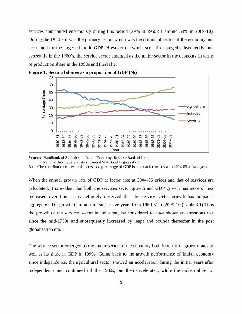
services contributed enormously during this period (29% in 1950-51 around 58% in 2009-10).

During the 1950‟s it was the primary sector which was the dominant sector of the economy and

accounted for the largest share in GDP. However the whole scenario changed subsequently, and

especially in the 1980‟s, the service sector emerged as the major sector in the economy in terms

of production share in the 1990s and thereafter.

Figure 1: Sectoral shares as a proportion of GDP (%)

Source: Handbook of Statistics on Indian Economy, Reserve Bank of India

National Accounts Statistics, Central Statistical Organisation

Note:The contribution of sectoral shares as a percentage of GDP is taken at factor costwith 2004-05 as base year.

When the annual growth rate of GDP at factor cost at 2004-05 prices and that of services are

calculated, it is evident that both the services sector growth and GDP growth has more or less

increased over time. It is definitely observed that the service sector growth has outpaced

aggregate GDP growth in almost all successive years from 1950-51 to 2009-10 (Table 3.1).Thus

the growth of the services sector in India may be considered to have shown an enormous rise

since the mid-1980s and subsequently increased by leaps and bounds thereafter in the post

globalisation era.

The service sector emerged as the major sector of the economy both in terms of growth rates as

well as its share in GDP in 1990s. Going back to the growth performance of Indian economy

since independence, the agricultural sector showed an acceleration during the initial years after

independence and continued till the 1980s, but then decelerated, while the industrial sector

0

10

20

30

40

50

60

70

19

50

-51

19

53

-54

19

56

-57

19

59

-60

19

62

-63

19

65

-66

19

68

-69

19

71

-72

19

74

-75

19

77

-78

19

80

-81

19

83

-84

19

86

-87

19

89

-90

19

92

-93

19

95

-96

19

98

-99

20

01

-02

20

04

-05

20

07

-08

Pe

rce

nta

ge S

har

e

Year

Agriculture

Industry

Services

10

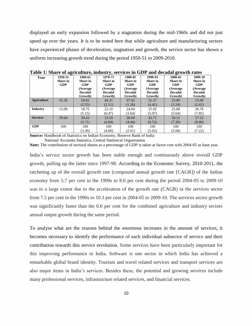
displayed an early expansion followed by a stagnation during the mid-1960s and did not just

speed up over the years. It is to be noted here that while agriculture and manufacturing sectors

have experienced phases of deceleration, stagnation and growth, the service sector has shown a

uniform increasing growth trend during the period 1950-51 to 2009-2010.

Table 1: Share of agriculture, industry, services in GDP and decadal growth rates Year 1950-51

Share in

GDP

1960-61

Share in

GDP

(Average

Decadal

Growth)

1970-71

Share in

GDP

(Average

Decadal

Growth)

1980-81

Share in

GDP

(Average

Decadal

Growth)

1990-91

Share in

GDP

(Average

Decadal

Growth)

2000-01

Share in

GDP

(Average

Decadal

Growth)

2009-10

Share in

GDP

(Average

Decadal

Growth)

Agriculture 55.28

50.81

(2.55)

44.31

(2.51)

37.92

(1.26)

31.37

(4.41)

23.89

(3.24)

15.68

(2.42) Industry 15.08

18.75

(5.15)

22.10

(6.47)

24.04

(3.64)

25.92

(5.97)

25.80

(5.64)

26.78

(7.85) Services 29.64

30.43

(3.71)

33.59

(4.84)

38.04

(4.44)

42.71

(6.53)

50.31

(7.28)

57.53

(8.80) GDP 100

100

(3.30)

100

(4.00)

100

(2.91)

100

(5.62)

100

(5.68)

100

(7.22)

Source: Handbook of Statistics on Indian Economy, Reserve Bank of India

National Accounts Statistics, Central Statistical Organisation

Note: The contribution of sectoral shares as a percentage of GDP is taken at factor cost with 2004-05 as base year.

India‟s service sector growth has been stable enough and continuously above overall GDP

growth, pulling up the latter since 1997-98. According to the Economic Survey, 2010-2011, the

ratcheting up of the overall growth rate (compound annual growth rate [CAGR]) of the Indian

economy from 5.7 per cent in the 1990s to 8.6 per cent during the period 2004-05 to 2009-10

was to a large extent due to the acceleration of the growth rate (CAGR) in the services sector

from 7.5 per cent in the 1990s to 10.3 per cent in 2004-05 to 2009-10. The services sector growth

was significantly faster than the 6.6 per cent for the combined agriculture and industry sectors

annual output growth during the same period.

To analyse what are the reasons behind the enormous increases in the amount of services, it

becomes necessary to identify the performance of each individual subsector of service and their

contribution towards this service revolution. Some services have been particularly important for

this improving performance in India. Software is one sector in which India has achieved a

remarkable global brand identity. Tourism and travel related services and transport services are

also major items in India‟s services. Besides these, the potential and growing services include

many professional services, infrastructure related services, and financial services.

11

The emergence of services as the most dynamic sector in the Indian economy has in many ways

been a revolution. The various subsectors that comprises of the services sector, their respective

share in services GDP, their average annual growth rates gives us an illustration of which of the

subsector of services is growing fast and which isn‟t. In India, the national income classification

given by Central Statistical Organisation is followed. In the National Income Accounting in

India, service sector includes the following:

(1) Trade, hotels and restaurants (THR)

(2) Transport, storage and communication

(3) Financing, Insurance, Real Estate and Business Services

(4) Community, Social and Personal services

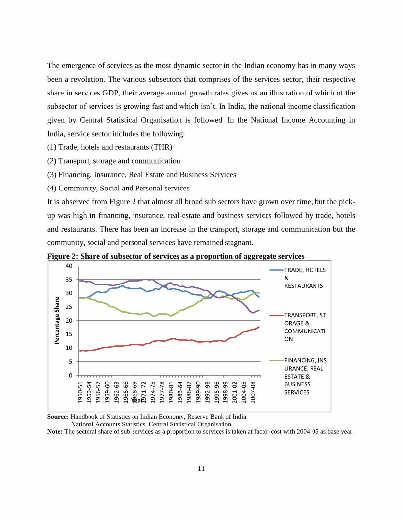
It is observed from Figure 2 that almost all broad sub sectors have grown over time, but the pick-

up was high in financing, insurance, real-estate and business services followed by trade, hotels

and restaurants. There has been an increase in the transport, storage and communication but the

community, social and personal services have remained stagnant.

Figure 2: Share of subsector of services as a proportion of aggregate services

Source: Handbook of Statistics on Indian Economy, Reserve Bank of India

National Accounts Statistics, Central Statistical Organisation.

Note: The sectoral share of sub-services as a proportion to services is taken at factor cost with 2004-05 as base year.

0

5

10

15

20

25

30

35

40

19

50

-51

19

53

-54

19

56

-57

19

59

-60

19

62

-63

19

65

-66

19

68

-69

19

71

-72

19

74

-75

19

77

-78

19

80

-81

19

83

-84

19

86

-87

19

89

-90

19

92

-93

19

95

-96

19

98

-99

20

01

-02

20

04

-05

20

07

-08

Pe

rce

nta

ge S

har

e

Year

TRADE, HOTELS & RESTAURANTS

TRANSPORT, STORAGE & COMMUNICATION

FINANCING, INSURANCE, REAL ESTATE & BUSINESS SERVICES

12

A clearer view is observed when we consider the share of the subsectors of services in services

GDP at factor cost at 2004-05 prices. Figure 2 shows that the share of subsectors like trade hotel

and restaurants have remained more or less consistent over the period from 1950-51 to 2009-10.

The share of transport, storage and communication has increased many fold i.e from 8.88% in

1950-51 to 17.73% in 2009-10. The share of financing, real estate have increased over the period

under consideration with a decrease somewhere in between, but it has captured almost 30% share

of the service sector over the years. The share of community, social and personal services,

however, has shown a considerable decrease over the concerned period. It has somewhat

decreased from 35% from 1950-51 to 23% in 2009-10. This sector which happened to be the

main foundation of service sector mainly growth of services during the 1950s happened to have

lost its importance in terms of productivity especially during the post-globalisation era.

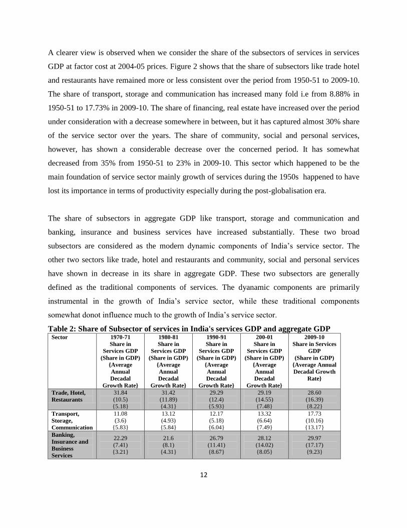
The share of subsectors in aggregate GDP like transport, storage and communication and

banking, insurance and business services have increased substantially. These two broad

subsectors are considered as the modern dynamic components of India‟s service sector. The

other two sectors like trade, hotel and restaurants and community, social and personal services

have shown in decrease in its share in aggregate GDP. These two subsectors are generally

defined as the traditional components of services. The dyanamic components are primarily

instrumental in the growth of India‟s service sector, while these traditional components

somewhat donot influence much to the growth of India‟s service sector.

Table 2: Share of Subsector of services in India's services GDP and aggregate GDP Sector 1970-71

Share in

Services GDP

(Share in GDP)

{Average

Annual

Decadal

Growth Rate}

1980-81

Share in

Services GDP

(Share in GDP)

{Average

Annual

Decadal

Growth Rate}

1990-91

Share in

Services GDP

(Share in GDP)

{Average

Annual

Decadal

Growth Rate}

200-01

Share in

Services GDP

(Share in GDP)

{Average

Annual

Decadal

Growth Rate}

2009-10

Share in Services

GDP

(Share in GDP)

{Average Annual

Decadal Growth

Rate}

Trade, Hotel,

Restaurants

31.84

(10.5)

{5.18}

31.42

(11.89)

{4.31}

29.29

(12.4)

{5.93}

29.19

(14.55)

{7.48}

28.60

(16.39)

{8.22}

Transport,

Storage,

Communication

11.08

(3.6)

{5.83}

13.12

(4.93)

{5.84}

12.17

(5.18)

{6.04}

13.32

(6.64)

{7.49}

17.73

(10.16)

{13.17}

Banking,

Insurance and

Business

Services

22.29

(7.41)

{3.21}

21.6

(8.1)

{4.31}

26.79

(11.41)

{8.67}

28.12

(14.02)

{8.05}

29.97

(17.17)

{9.23}

13

Community,

Social and

Personal

services

34.77

(11.56)

{5.24}

33.81

(12.73)

{4.13}

31.73

(13.51)

{5.90}

29.35

(14.63)

{6.46}

23.68

(13.56)

{6.77}

Source: Handbook of Statistics on Indian Economy, Reserve Bank of India

National Accounts Statistics, Central Statistical Organisation. Note: The share and growth of subsector of services in services and GDP is calculated with 2004-05 as base year.

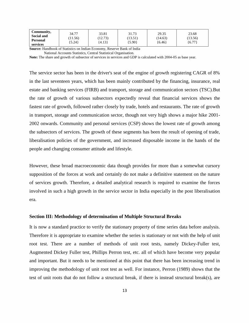
The service sector has been in the driver's seat of the engine of growth registering CAGR of 8%

in the last seventeen years, which has been mainly contributed by the financing, insurance, real

estate and banking services (FIRB) and transport, storage and communication sectors (TSC).But

the rate of growth of various subsectors expectedly reveal that financial services shows the

fastest rate of growth, followed rather closely by trade, hotels and restaurants. The rate of growth

in transport, storage and communication sector, though not very high shows a major hike 2001-

2002 onwards. Community and personal services (CSP) shows the lowest rate of growth among

the subsectors of services. The growth of these segments has been the result of opening of trade,

liberalisation policies of the government, and increased disposable income in the hands of the

people and changing consumer attitude and lifestyle.

However, these broad macroeconomic data though provides for more than a somewhat cursory

supposition of the forces at work and certainly do not make a definitive statement on the nature

of services growth. Therefore, a detailed analytical research is required to examine the forces

involved in such a high growth in the service sector in India especially in the post liberalisation

era.

Section III: Methodology of determination of Multiple Structural Breaks

It is now a standard practice to verify the stationary property of time series data before analysis.

Therefore it is appropriate to examine whether the series is stationary or not with the help of unit

root test. There are a number of methods of unit root tests, namely Dickey-Fuller test,

Augmented Dickey Fuller test, Phillips Perron test, etc. all of which have become very popular

and important. But it needs to be mentioned at this point that there has been increasing trend in

improving the methodology of unit root test as well. For instance, Perron (1989) shows that the

test of unit roots that do not follow a structural break, if there is instead structural break(s), are

14

biased in favour of non-stationarity. Therefore it is necessary to examine whether any structural

break is present in the series.

The three steps involved in the whole exercise of estimating the time trend of services. First, the

structural break test has been tested for the data series on services following the methodology

suggested by Bai and Perron (1998). Then the presence of unit root with structural break

including the break point has been tested using the methods suggested by Banerjee, Lumsdaine

and Papell (1992) and Lumsdaine and Stock (1997). Finally the trend growth rate of GDP,

services and sub-sectoral services are estimated using the Boyce (1986) method in various sub-

periods.

Test for structural Break: Bai-Perron Test

Both the statistics and economics literature contains a vast amount of work on the issues related

to structural change, most of it specifically designed for the case of a single change. But most

macroeconomic time series usually can contain more than one structural break. The

econometrics literature has witnessed recently an upsurge of interest in extending procedure to

various models with unknown breakpoint. With respect to the problem of testing for structural

change, recent contribution include the treatment by Andrews (1993a, 1993b), Andrews, Lee, &

Ploberger (1994, 1996) and Bai and Perron (1998,2003). In this section, the Bai and Perron

(1998) method in order to examine if there are any structural break in the series. To that effect,

Bai and Perron (1998) recently provide a comprehensive analysis of several issues in the context

of multiple structural change models and develop some tests which preclude the presence of

trending regressors. This test is helpful in the changes present and also it endogenously

determines the points of break with no prior knowledge.

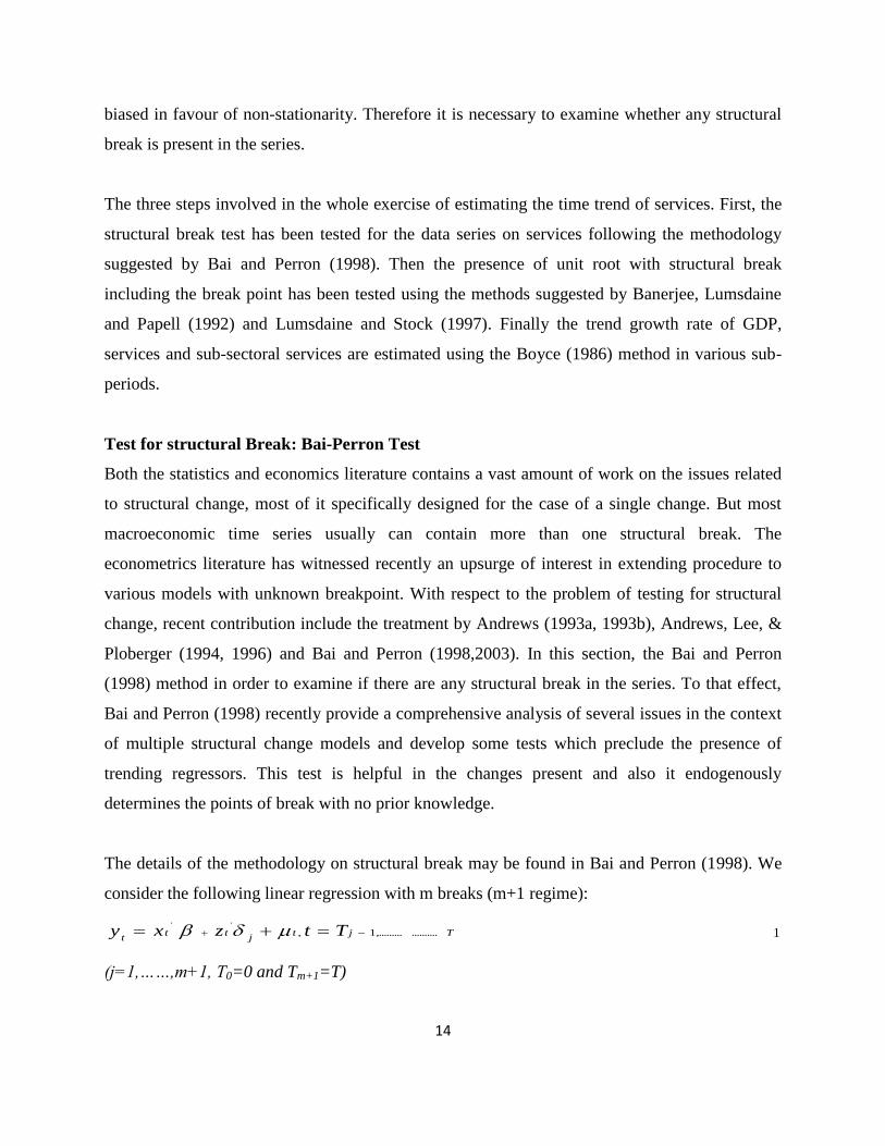
The details of the methodology on structural break may be found in Bai and Perron (1998). We

consider the following linear regression with m breaks (m+1 regime):

Tjtj

ttt

Ttzxy ..........,.........1,''

1

(j=1,……,m+1, T0=0 and Tm+1=T)

15

where yt is the observed dependent variable, xtp

and ztq

are vectors of covariates, β and

δj are the corresponding vectors of coefficients with δi δi+1 )1( mi and µt is the error term at

time t. The break dates (T1,….,Tm) are explicitly regarded as unknown. It may be noted that this

is a partial structural change model insofar as β doesn‟t shift and is effectively estimated over the

entire sample. Then the purpose is to estimate the unknown regression coefficients and the break

dates, that is to say (β, δ1 ,…… δm+1, T1,….,Tm), when T observations on (yt ,xt, zt) are available.

Note that this is a partial change model in the sense that β is not subject to shifts and is

effectively estimated using the entire sample.

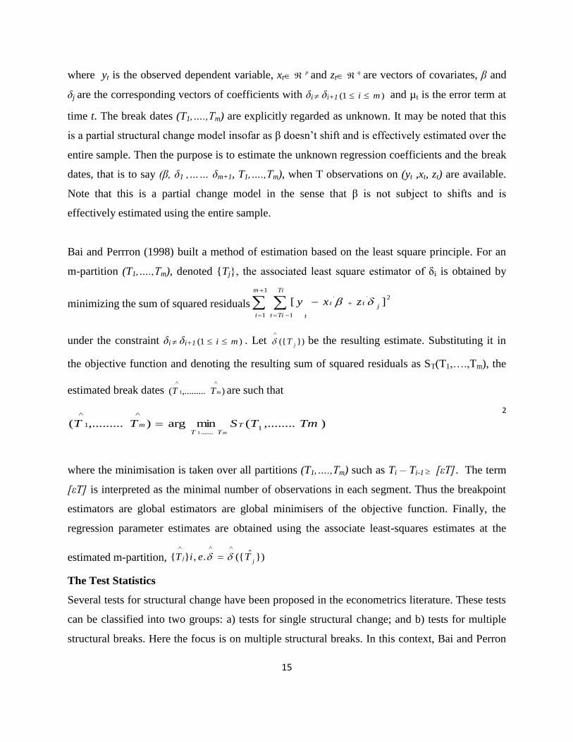
Bai and Perrron (1998) built a method of estimation based on the least square principle. For an

m-partition (T1,….,Tm), denoted {Tj}, the associated least square estimator of δi is obtained by

minimizing the sum of squared residuals2

1

1 1

][''

jtt

t

m

i

Ti

Tit

zxy

under the constraint δi δi+1 )1( mi . Let })({j

T

be the resulting estimate. Substituting it in

the objective function and denoting the resulting sum of squared residuals as ST(T1,….,Tm), the

estimated break dates ),.........( 1

mTT are such that

2

where the minimisation is taken over all partitions (T1,….,Tm) such as Ti – Ti-1 [εT]. The term

[εT] is interpreted as the minimal number of observations in each segment. Thus the breakpoint

estimators are global estimators are global minimisers of the objective function. Finally, the

regression parameter estimates are obtained using the associate least-squares estimates at the

estimated m-partition, })ˆ({.,}{j

j TeiT

The Test Statistics

Several tests for structural change have been proposed in the econometrics literature. These tests

can be classified into two groups: a) tests for single structural change; and b) tests for multiple

structural breaks. Here the focus is on multiple structural breaks. In this context, Bai and Perron

),........(minarg),.........(1

.......

1

1

TmTSTT T

TT

m

m

16

(1998) consider estimating multiple structural changes in the linear model and developed three

tests.

Test of Structural Stability versus an Unknown Number of Breaks

Bai and Perron (1998) also consider tests of no structural change against an unknown number of

breaks given some upper bound M for m. The following new class of tests is called double

maximum tests and is defined for some fixed weights {a1…………am} as

):1

1

1

),........1(1

1

ˆ,........ˆ(max

):,........(max).........,.........,,(max

qMTm

Mm

MT

m

m

Mm

MT

Fa

qFSupaaaqMFD

3

The weights {a1..........am} reflect the imposition of some priors on the likelihood of various

numbers of structural breaks. Firstly, they set all weights equal to unity, i.e. am=1 and label this

version of the test as UDmaxFT(M,q). Then they consider a set of weights that the marginal p-

values are equal across values of m. The weights are then defined as a1=1 and am= c(q, α, 1)/c(q,

α, m) for m>1, where α is the significance level of the test and c(q, α, m) is the asymptotic

critical value of the test ):,........():,........(sup 11 qFqF nTnT . This version of the test is

denoted as WD maxFT(M, q).

A Sequential Test

The last test developed by Bai and Perron (1998)is a sequential test of l versus l+1 structural

change:

2..............,.........11

11

1 ˆ/)}.,,.......,(infmin),........({)/1(sup,

lT

li

lTT TiTTSTTSllFi

3.4

where,

},)()(;{ 111,

llllllni

TTTTTT

).,,.......,( .......................,11 liT

TTiTTS

is the sum of squared residuals resulting from the least squares

estimation from each m-partition (T1,……………..Tm) and 2

is a consistent estimator of 2

under the null hypothesis.

The asymptotic distributions of these three tests are derived inBai and Perron (1998) and the

asymptotic critical values are tabulated in Bai and Perron (1998, 1993) for ε = 0.05 (M=9), 0.10

(M=8), 0.15(M =5), 0.20(M=3), and 0.25 (M=2).

17

Selection Procedure

A preferred strategy to determine the number of breaks in a set of data is to first look at the

UDmaxFT(M,q) test to see if at least a structural break exists. The number of breaks can then be

decided based upon an examination of the supFT (l+1/l) statistics constructed using the break date

estimates obtained from a global minimisation of the sum of squared residuals (i.e. m breaks are

selected such that the tests supFT (l+1/l) are non-significant for any l>m). Bai and Perron (2003)

conclude that this method leads to the best results and is recommended for empirical

applications. Further if the estimation allows for a change in all the parameters i.e. the intercept

and the slope it is said to be a pure structural break model.

Kinked Exponential Models for Growth Rate Estimation

Next, after having determined the breakpoints by the Bai and Perron (1998) test, the calculations

of the sub-period growth rates are examined using the kinked semi-logarithmic trend equation

used by Boyce (1986). The usual technique for estimating growth rates in the sub-periods of a

time series is to fit separate exponential trend lines by ordinary least squares to each segment of

the series. These trend lines are likely to be discontinuous, which can result in anomalies such as

sub-period growth rates which can exceed, or are less than, the estimated growth rate for the

period as a whole. Discontinuities between segments of a piece-wise regression can be

eliminated via the imposition of linear restrictions. In the case of log-linear models, such an

approach yields kinked exponential functions which provide a better basis than conventional

estimates for intertemporal and cross-sectional growth rate comparisons. Kinked exponential

models with one, two and multiple kink points are derived. These can be easily estimated with

standard OLS regression packages by using composite independent variables.

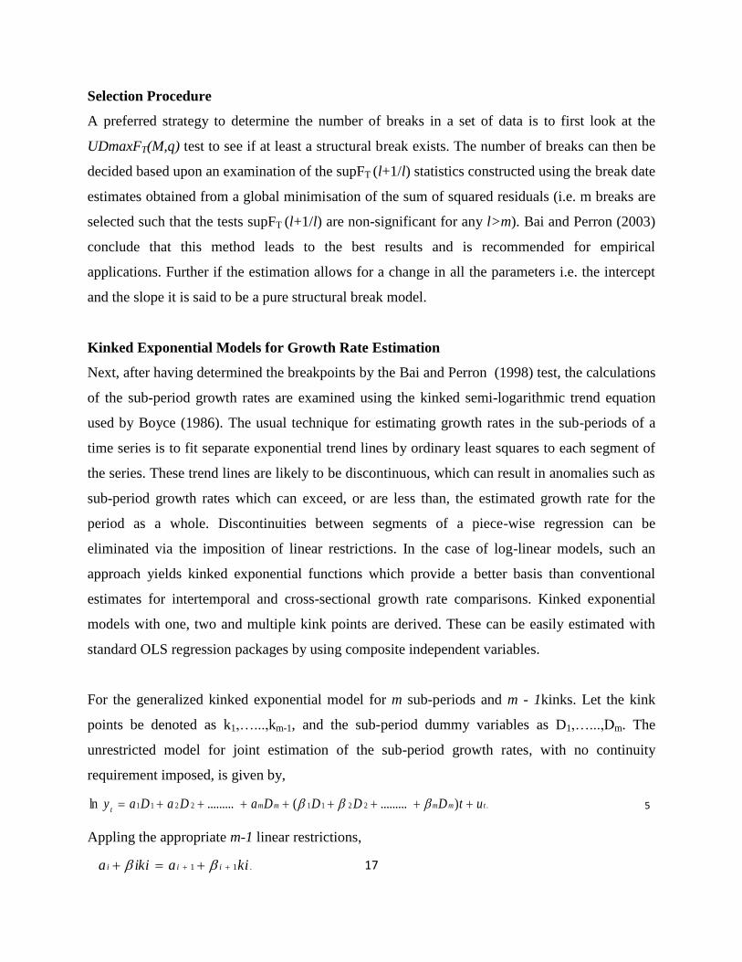
For the generalized kinked exponential model for m sub-periods and m - 1kinks. Let the kink

points be denoted as k1,…...,km-1, and the sub-period dummy variables as D1,…...,Dm. The

unrestricted model for joint estimation of the sub-period growth rates, with no continuity

requirement imposed, is given by,

.22112211 ).........(.........ln tmmmmt

utDDDDaDaDay

5

Appling the appropriate m-1 linear restrictions,

.11 kiaikia iii

18

for all 1,......,2,1 mi 6

we obtain the generalized kinked exponential model:

.1

1

1

1 2 3

21221111

)(.........)(

.........)()(ln

tmmmm

m

ij

m

ij

ijijii

m

j

m

j

m

j

jjjt

ukDtDkDkDtD

kDkDtDkDtDay

7

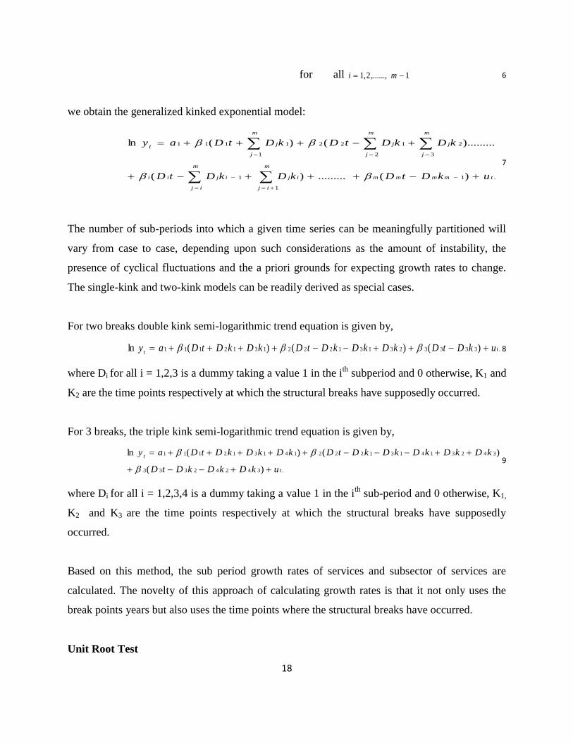
The number of sub-periods into which a given time series can be meaningfully partitioned will

vary from case to case, depending upon such considerations as the amount of instability, the

presence of cyclical fluctuations and the a priori grounds for expecting growth rates to change.

The single-kink and two-kink models can be readily derived as special cases.

For two breaks double kink semi-logarithmic trend equation is given by,

.3333231312221312111 )()()(ln tt

ukDtDkDkDkDtDkDkDtDay 8

where Di for all i = 1,2,3 is a dummy taking a value 1 in the i

th subperiod and 0 otherwise, K1 and

K2 are the time points respectively at which the structural breaks have supposedly occurred.

For 3 breaks, the triple kink semi-logarithmic trend equation is given by,

.34242333

342314131222141312111

)(

)()(ln

t

t

ukDkDkDtD

kDkDkDkDkDtDkDkDkDtDay

9

where Di for all i = 1,2,3,4 is a dummy taking a value 1 in the ith

sub-period and 0 otherwise, K1,

K2 and K3 are the time points respectively at which the structural breaks have supposedly

occurred.

Based on this method, the sub period growth rates of services and subsector of services are

calculated. The novelty of this approach of calculating growth rates is that it not only uses the

break points years but also uses the time points where the structural breaks have occurred.

Unit Root Test

19

Unit root tests are based on the implicit assumption that the deterministic trend is correctly

specified. Unit root tests, namely DF test, ADF test, PP test, etc are important but there has been

increasing trend in improving the methodology of unit root test as well. Nelson and Plosser

(1982) found evidence that in favour of unit root hypothesis for 13 out of 14 long-term annual

macro series. Perron(1989) suggested that the observed unit root behaviour have been a failure to

account for any structural break in the data. Perron(1989) argued that if there is a break in the

deterministic trend, the unit root test‟s results are misleading, i.e., under the break the unit root

tests can treat trend stationary process as a difference stationary process. Perron(1989) develops

a method of test of unit roots in the presence of structural break. The analysis was done with an

exogenous break. Accordingly, he challenged the findings of Nelson and Plosser (1982) and he

reversed the Nelson and Plosser conclusions of 10 f the 11 series. Perron‟s paper started a

controversy about the effect of trend breaks on unit root tests and again his study was criticized

on the ground that he assumed the break point to be known.

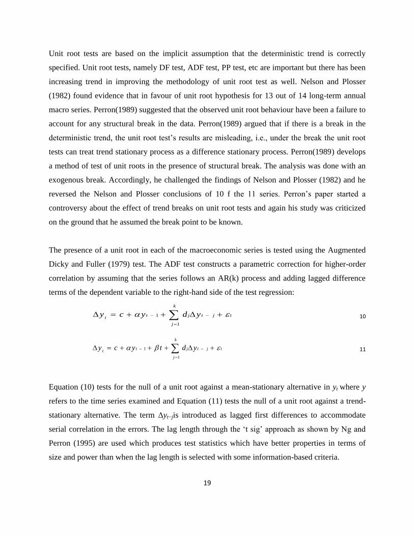
The presence of a unit root in each of the macroeconomic series is tested using the Augmented

Dicky and Fuller (1979) test. The ADF test constructs a parametric correction for higher-order

correlation by assuming that the series follows an AR(k) process and adding lagged difference

terms of the dependent variable to the right-hand side of the test regression:

t

k

j

jtjtt

ydycy

1

1

10

t

k

j

jtjtt

ydtycy

1

1

11

Equation (10) tests for the null of a unit root against a mean-stationary alternative in yt where y

refers to the time series examined and Equation (11) tests the null of a unit root against a trend-

stationary alternative. The term Δyt−jis introduced as lagged first differences to accommodate

serial correlation in the errors. The lag length through the „t sig‟ approach as shown by Ng and

Perron (1995) are used which produces test statistics which have better properties in terms of

size and power than when the lag length is selected with some information-based criteria.

20

Further, Zivot and Andrews (1992) and Banerjee, Lumsdaine and Stock (1992) tested for unit

root incorporated an endogenous break point into the model specification and they showed

Perron‟s conclusions are reversed. Zivot and Andrews(1992) use a sequential test, derive the

asymptotic distribution, they fail to reject the unit root hypothesis for four of ten series for which

Perron rejected the unit root null. Banerjee, Lumsdaine and Stock (1992) (BLS, henceforth)

apply a variety of recursive, rolling and sequential tests endogenising the break point to different

international data. For the present study this BLS test for unit root is used. Here it can be

mentioned this test cannot be used to find the break point, or whether there is any break in the

series at all. This test can be used to test the unit root hypothesis independent of structural break.

The power and size consideration of this BLS test has been given in their paper.

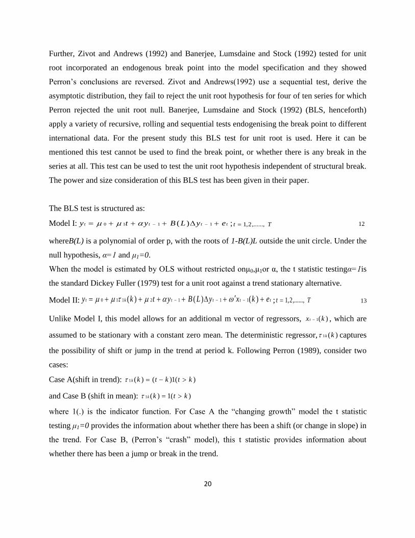
The BLS test is structured as:

Model I: tttt eyLByty 1110 )( ; Tt ,......,2,1 12

whereB(L) is a polynomial of order p, with the roots of 1-B(L)L outside the unit circle. Under the

null hypothesis, α=1 and μ1=0.

When the model is estimated by OLS without restricted onμ0,μ1or α, the t statistic testingα=1is

the standard Dickey Fuller (1979) test for a unit root against a trend stationary alternative.

Model II: ttttkt ekxyLBytky )()()( 1112110 ; Tt ,......,2,1 13

Unlike Model I, this model allows for an additional m vector of regressors, )(1 kx t , which are

assumed to be stationary with a constant zero mean. The deterministic regressor, )(1 kk captures

the possibility of shift or jump in the trend at period k. Following Perron (1989), consider two

cases:

Case A(shift in trend): )(1)()(1 ktktkk

and Case B (shift in mean): )(1)(1 ktkk

where 1(.) is the indicator function. For Case A the “changing growth” model the t statistic

testing μ1=0 provides the information about whether there has been a shift (or change in slope) in

the trend. For Case B, (Perron‟s “crash” model), this t statistic provides information about

whether there has been a jump or break in the trend.

21

Based on different tests used, three test statistics are examined under recursive tests. These are

the maximum Dickey- Fuller statistic, )(ˆmaxˆ0

max

T

ktt

DFTkkDF ; and the minimal Dickey Fuller

Statistic )(ˆminˆ0

min

T

ktt

DFTkkDF ; and

minmax ˆˆˆDFDF

diff

DFttt . For these, )(ˆ

T

kt

DF, that is the full

sample Dickey Fuller statistic is computed as the t statistic testing α=1in the regression estimated

over kt ,......,2,1 .Given the presence of breakpoints confirmed by Bai-Perron test and the

presence of unit roots confirmed by the BLS test, the presence of unit root in the presence of

structural break is ascertained by an extension of the Zivot and Andrews (1992), i.e. the

Lumsdaine and Papell (1997) test, where break dates are not determined exogenously.

Lumsdaine and Papell (1997) (LP hereafter) extended the Zivot and Andrews methodology of

two breaks. The methodology can be extended to three or more breaks.

As illustrated by the above equations, a constant and a linear time trend in ADF test regression is

selected to be included. Phillips and Perron (1988) propose an alternative (nonparametric)

method of controlling for serial correlation when testing for a unit root. The PP method estimates

the non-augmented DF test equation [Equation (10) and (11) without

k

j

jtj yd

1

term on RHS],

and modifies the t-ratio of the α coefficient so that serial correlation does not affect the

asymptotic distribution of the test statistic. For comparison purposes, we also perform the PP

tests and report their results in addition to the generally favoured ADF test.

A problem common with the conventional unit root tests such as the ADF, DF-GLS and PP tests,

is that they do not allow for the possibility of a structural break. Assuming the time of the break

as an exogenous phenomenon, Perron showed that the power to reject a unit root decreases when

the stationary alternative is true and a structural break is ignored.

Zivot and Andrews (1992) proposed a variation of Perron‟s original test in which they assume

that the exact time of the break-point is unknown. Instead a data dependent algorithm is used to

proxy Perron‟s subjective procedure to determine the break points. Following Perron‟s

characterisation of the form of structural break, Zivot and Andrews proceeded with three models

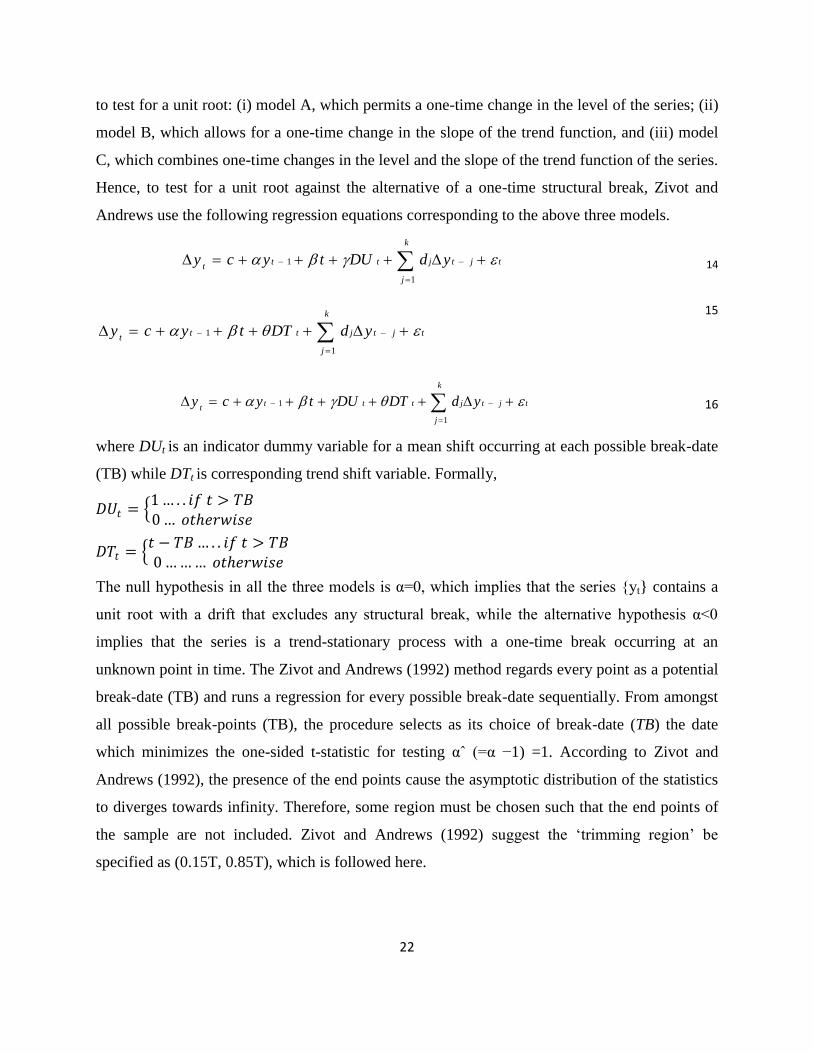
22

to test for a unit root: (i) model A, which permits a one-time change in the level of the series; (ii)

model B, which allows for a one-time change in the slope of the trend function, and (iii) model

C, which combines one-time changes in the level and the slope of the trend function of the series.

Hence, to test for a unit root against the alternative of a one-time structural break, Zivot and

Andrews use the following regression equations corresponding to the above three models.

t

k

j

jtjttt

ydDUtycy

1

1

14

15

t

k

j

jtjtttt

ydDTDUtycy

1

1

16

where DUt is an indicator dummy variable for a mean shift occurring at each possible break-date

(TB) while DTt is corresponding trend shift variable. Formally,

𝐷𝑈𝑡 = 1 … . . 𝑖𝑓 𝑡 > 𝑇𝐵0 … 𝑜𝑡ℎ𝑒𝑟𝑤𝑖𝑠𝑒

𝐷𝑇𝑡 = 𝑡 − 𝑇𝐵… . . 𝑖𝑓 𝑡 > 𝑇𝐵0 ……… 𝑜𝑡ℎ𝑒𝑟𝑤𝑖𝑠𝑒

The null hypothesis in all the three models is α=0, which implies that the series {yt} contains a

unit root with a drift that excludes any structural break, while the alternative hypothesis α<0

implies that the series is a trend-stationary process with a one-time break occurring at an

unknown point in time. The Zivot and Andrews (1992) method regards every point as a potential

break-date (TB) and runs a regression for every possible break-date sequentially. From amongst

all possible break-points (TB), the procedure selects as its choice of break-date (TB) the date

which minimizes the one-sided t-statistic for testing αˆ (=α −1) =1. According to Zivot and

Andrews (1992), the presence of the end points cause the asymptotic distribution of the statistics

to diverges towards infinity. Therefore, some region must be chosen such that the end points of

the sample are not included. Zivot and Andrews (1992) suggest the „trimming region‟ be

specified as (0.15T, 0.85T), which is followed here.

t

k

j

jtjttt

ydDTtycy

1

1

23

Lumsdaine and Papell (1997) test considers the behaviour of sequences of the Dickey-Fuller

(1979) t tests for a unit root. It is similar to the spirit to the sequential tests for changing in the

coefficients of BLS (1992), in case there is only one structural break. LP computed a statistic

using the full sample allowing two shifts in the deterministic trend at distinct unknown dates.

The model considered here is the extension of the Zivot Andrews model (Model C), using the

following equation:

17

where Tt ,......,2,1 and c(L) is the lag polynomial of unknown order k and 1-c(L)L has all its unit

roots outside the unit circle, the null hypothesis of non-stationarity is examined against the

alternative of stationary with two break. Here, DU1tand DU2t are the indicator dummies for a

mean shift occurring at times TB1 and TB2 respectively and DT1t and DT2t are the

corresponding trend shift variables. That is,

)1(11 TBtDU t ,

)2(12 TBtDU t ,

)1(1)1(1 TBtTBtDT t and )2(1)2(2 TBtTBtDT t

and k is the lag length decided on the basis of the AIC or SBC criteria. The test is extended to

three structural breaks, in this chapter.

Section IV: Results and Interpretation

In this section, the breakpoints in specialised services, services and GDP are estimated using this

methodology. For each individual variable, the model is characterized as:

Pure Structural break model: Tjtt

jjjt

Ttuytcy ..........,.........1,1

18

Partial Structural break model:Tjt

tjj

tTtuytcy ..........,.........1,

1

19

Therefore, the two structural breaks model differ in the way that in the generalized case, the

break is taken into consideration with a variable deterministic trend coefficient β and

autoregressive parameter ρ. The partial structural break model is restricted in the sense that it

assumes the autoregressive parameter, ρ, to be constant.

In order to detect for the structural breaks, the steps suggested by Bai and Perron stated above are

followed. First, the UDMAX and WDMAX statistics, which are double maximum tests, where

the null hypothesis of no structural breaks is tests against the alternative of an unknown number

t

k

i

ititttttt ycyDTDUDTDUty

1

1221

24

of breaks, are calculated. As stated above, the tests are used to determine if at least one structural

break is present. Subsequently, the sup FT(0|l) which is a series of Wald tests for hypothesis of 0

breaks vs. l breaks are calculated. In the implementation of the procedure, a maximum up to 4

breaks is allowed and a trimming ε=0.05 which corresponds to each segment having at least 12

observations. If these tests show evidence of at least one structural break, then the number of

breaks can be determined by the SupF(l+1/l). If the test is significant at the 5 per cent level, l+1

breaks are chosen.

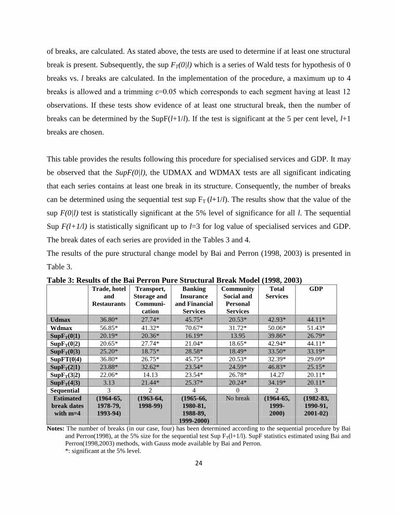
This table provides the results following this procedure for specialised services and GDP. It may

be observed that the SupF(0|l), the UDMAX and WDMAX tests are all significant indicating

that each series contains at least one break in its structure. Consequently, the number of breaks

can be determined using the sequential test sup FT (l+1/l). The results show that the value of the

sup F(0|l) test is statistically significant at the 5% level of significance for all l. The sequential

Sup F(l+1/l) is statistically significant up to l=3 for log value of specialised services and GDP.

The break dates of each series are provided in the Tables 3 and 4.

The results of the pure structural change model by Bai and Perron (1998, 2003) is presented in

Table 3.

Table 3: Results of the Bai Perron Pure Structural Break Model (1998, 2003)

Trade, hotel

and

Restaurants

Transport,

Storage and

Communi-

cation

Banking

Insurance

and Financial

Services

Community

Social and

Personal

Services

Total

Services

GDP

Udmax 36.80* 27.74* 45.75* 20.53* 42.93* 44.11*

Wdmax 56.85* 41.32* 70.67* 31.72* 50.06* 51.43*

SupFT(0|1) 20.19* 20.36* 16.19* 13.95 39.86* 26.79*

SupFT(0|2) 20.65* 27.74* 21.04* 18.65* 42.94* 44.11*

SupFT(0|3) 25.20* 18.75* 28.58* 18.49* 33.50* 33.19*

SupFT(0|4) 36.80* 26.75* 45.75* 20.53* 32.39* 29.09*

SupFT(2|1) 23.88* 32.62* 23.54* 24.59* 46.83* 25.15*

SupFT(3|2) 22.06* 14.13 23.54* 26.78* 14.27 20.11*

SupFT(4|3) 3.13 21.44* 25.37* 20.24* 34.19* 20.11*

Sequential 3 2 4 0 2 3

Estimated

break dates

with m=4

(1964-65,

1978-79,

1993-94)

(1963-64,

1998-99)

(1965-66,

1980-81,

1988-89,

1999-2000)

No break (1964-65,

1999-

2000)

(1982-83,

1990-91,

2001-02)

Notes: The number of breaks (in our case, four) has been determined according to the sequential procedure by Bai

and Perron(1998), at the 5% size for the sequential test Sup FT(l+1/l). SupF statistics estimated using Bai and

Perron(1998,2003) methods, with Gauss mode available by Bai and Perron.

*: significant at the 5% level.

25

The results of the pure break model reveal that the first break in India‟s GDP occurred at 1982-

83. The next two breaks as evident from economic policy change in India are at 1990-91 and

2001-02. However, the first break in the subsector of services and aggregate services as a whole

comes within the period 1963-1966, with the community, social and personal services sector

exhibiting no such break. This confirms the fact that the break in services GDP came long before

the break in GDP. It also points out that the service sector in India is not necessarily led by

economic reforms of 1991. The second break in services occurred at the beginning of the new

millennium, almost after a decade of the initiation of the reforms. However, it needs to be

mentioned that an aggregation of these services actually does not give a lucid picture because of

the diverse nature and the significance of the different subsector of services in the development

of the country. It is better to consider each of the sub-sectors of services individually and see

their growth pattern.

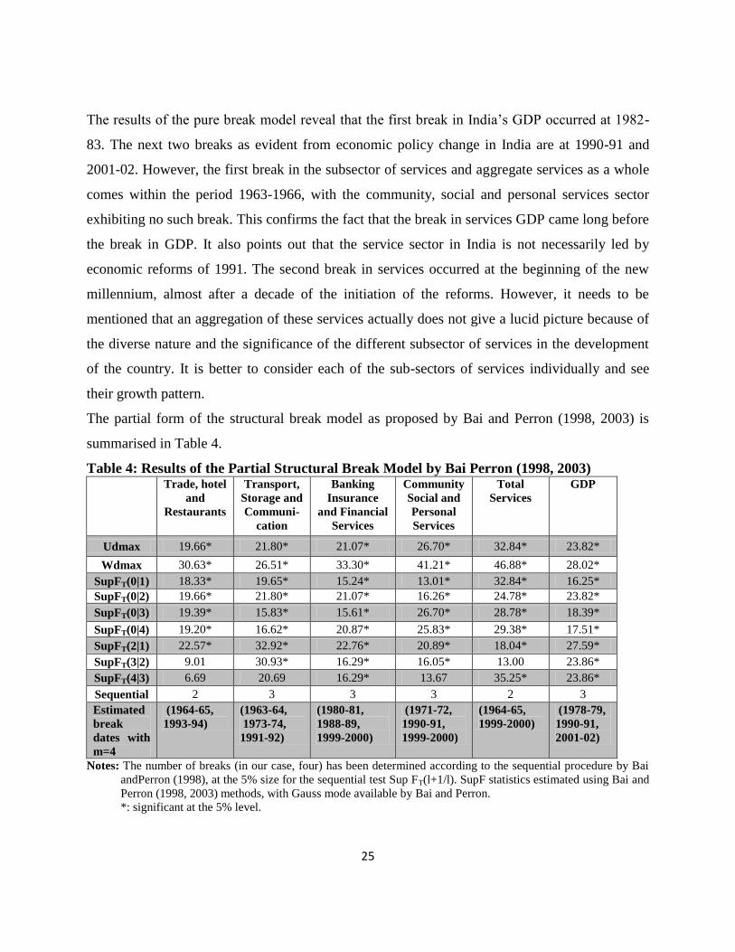
The partial form of the structural break model as proposed by Bai and Perron (1998, 2003) is

summarised in Table 4.

Table 4: Results of the Partial Structural Break Model by Bai Perron (1998, 2003) Trade, hotel

and

Restaurants

Transport,

Storage and

Communi-

cation

Banking

Insurance

and Financial

Services

Community

Social and

Personal

Services

Total

Services

GDP

Udmax 19.66* 21.80* 21.07* 26.70* 32.84* 23.82*

Wdmax 30.63* 26.51* 33.30* 41.21* 46.88* 28.02*

SupFT(0|1) 18.33* 19.65* 15.24* 13.01* 32.84* 16.25*

SupFT(0|2) 19.66* 21.80* 21.07* 16.26* 24.78* 23.82*

SupFT(0|3) 19.39* 15.83* 15.61* 26.70* 28.78* 18.39*

SupFT(0|4) 19.20* 16.62* 20.87* 25.83* 29.38* 17.51*

SupFT(2|1) 22.57* 32.92* 22.76* 20.89* 18.04* 27.59*

SupFT(3|2) 9.01 30.93* 16.29* 16.05* 13.00 23.86*

SupFT(4|3) 6.69 20.69 16.29* 13.67 35.25* 23.86*

Sequential 2 3 3 3 2 3

Estimated

break

dates with

m=4

(1964-65,

1993-94)

(1963-64,

1973-74,

1991-92)

(1980-81,

1988-89,

1999-2000)

(1971-72,

1990-91,

1999-2000)

(1964-65,

1999-2000)

(1978-79,

1990-91,

2001-02)

Notes: The number of breaks (in our case, four) has been determined according to the sequential procedure by Bai

andPerron (1998), at the 5% size for the sequential test Sup FT(l+1/l). SupF statistics estimated using Bai and

Perron (1998, 2003) methods, with Gauss mode available by Bai and Perron.

*: significant at the 5% level.

26

The results of the pure and partial structural tests appear somewhat similar, except for

community, social and personal services (CSP), which has no break in the pure form but has

three breaks in the partial form. For the rest, for example trade, hotel and restaurants, the first

break and the last break is in the same year, except that there is another break at 1978-79 in the

case of a pure structural break. Again for the banking, insurance and the financial services the

first break occurs at 1965-66 in the pure form, all the other three breaks are same in both pure

and partial models. For GDP, the first structural break occurs at 1982-83 in the pure form while

it occurs at 1978-79 in the partial form, the rest of the breakpoints being similar in both the

models. The partial structure of the model is taken for further analysis as in this model not all

parameters are subject to shifts, it considers only the change of intercept. The results are found to

be consistent with that of the economic policy of India. Following the tables, it is evident that the

first structural change is India‟s GDP growth has been brought about in 1978-79, whereas the

break in aggregate services sector has occurred much earlier in 1965-66. However, services

being so diverse in nature, aggregate services do not really match with the time at which the first

break in GDP occurred. But, the break in 1965-66 is brought about by a break in trade, hotel and

restaurants and transport, storage and communication and community, social and personal

services. The first break in financial services is somewhat commensurate with the time of break

with that of GDP.

Several studies like Nagraj(1990,1991), Dholakia(1994), Panagariya(2004), Wallack (2004),

Nayyar (2006), Balakrishnan and Permeshwaran (2007), Dholakia (2007) have addressed the

problem of estimation of structural break in the long term trend growth of the Indian economy at

the aggregate and the sectoral level. Our results are found to be similar with the growth of GDP

in India by Balakrishnan and Permeshwaran (2007). Our results have been little different from

their results because of a different base year period and the length of the period under study.

Even Wallack (2004) found that the first structural break in India‟s GDP growth rate to be at

1980-81. However, a recent article by Dholakia & Sapre (2011) considers the endogenous

estimation of break dates is sensitive of changes in the base year and the length of the partition

using Bai Perron model.

27

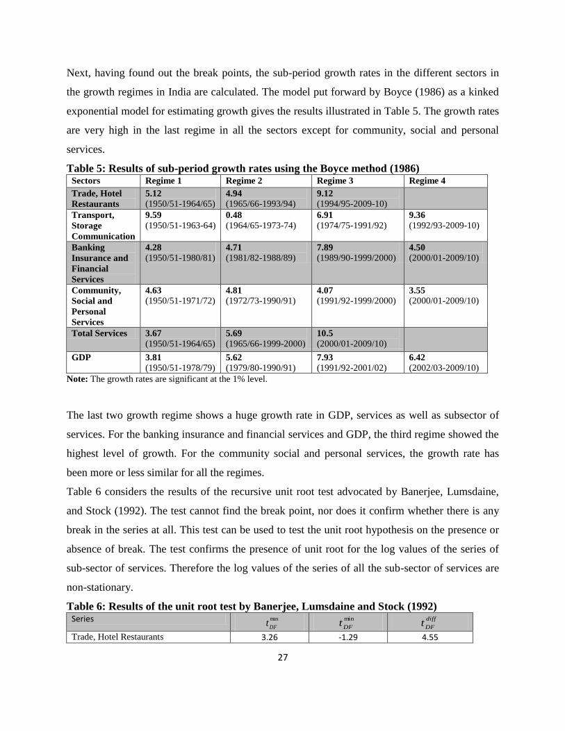
Next, having found out the break points, the sub-period growth rates in the different sectors in

the growth regimes in India are calculated. The model put forward by Boyce (1986) as a kinked

exponential model for estimating growth gives the results illustrated in Table 5. The growth rates

are very high in the last regime in all the sectors except for community, social and personal

services.

Table 5: Results of sub-period growth rates using the Boyce method (1986)

Sectors Regime 1 Regime 2 Regime 3 Regime 4

Trade, Hotel

Restaurants

5.12

(1950/51-1964/65) 4.94

(1965/66-1993/94) 9.12

(1994/95-2009-10)

Transport,

Storage

Communication

9.59

(1950/51-1963-64) 0.48

(1964/65-1973-74) 6.91

(1974/75-1991/92) 9.36

(1992/93-2009-10)

Banking

Insurance and

Financial

Services

4.28

(1950/51-1980/81) 4.71

(1981/82-1988/89) 7.89

(1989/90-1999/2000) 4.50

(2000/01-2009/10)

Community,

Social and

Personal

Services

4.63

(1950/51-1971/72) 4.81

(1972/73-1990/91) 4.07

(1991/92-1999/2000) 3.55

(2000/01-2009/10)

Total Services 3.67

(1950/51-1964/65) 5.69

(1965/66-1999-2000) 10.5

(2000/01-2009/10)

GDP 3.81 (1950/51-1978/79)

5.62 (1979/80-1990/91)

7.93 (1991/92-2001/02)

6.42 (2002/03-2009/10)

Note: The growth rates are significant at the 1% level.

The last two growth regime shows a huge growth rate in GDP, services as well as subsector of

services. For the banking insurance and financial services and GDP, the third regime showed the

highest level of growth. For the community social and personal services, the growth rate has

been more or less similar for all the regimes.

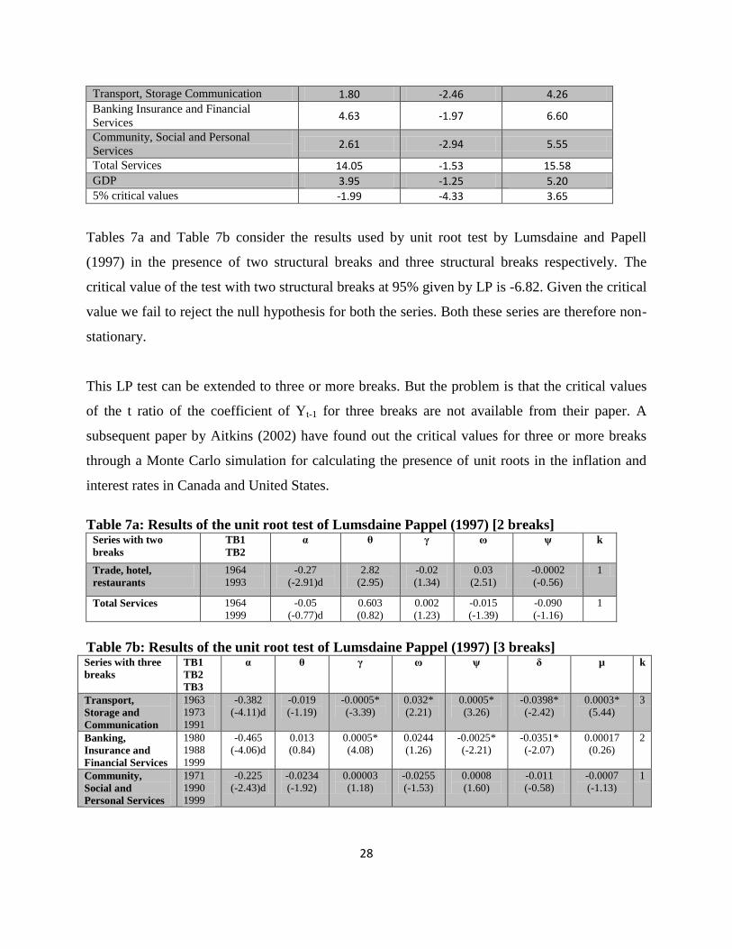
Table 6 considers the results of the recursive unit root test advocated by Banerjee, Lumsdaine,

and Stock (1992). The test cannot find the break point, nor does it confirm whether there is any

break in the series at all. This test can be used to test the unit root hypothesis on the presence or

absence of break. The test confirms the presence of unit root for the log values of the series of

sub-sector of services. Therefore the log values of the series of all the sub-sector of services are

non-stationary.

Table 6: Results of the unit root test by Banerjee, Lumsdaine and Stock (1992) Series max

DFt min

DFt

diff

DFt

Trade, Hotel Restaurants 3.26 -1.29 4.55

28

Transport, Storage Communication 1.80 -2.46 4.26 Banking Insurance and Financial

Services 4.63 -1.97 6.60

Community, Social and Personal

Services 2.61 -2.94 5.55

Total Services 14.05 -1.53 15.58 GDP 3.95 -1.25 5.20 5% critical values -1.99 -4.33 3.65

Tables 7a and Table 7b consider the results used by unit root test by Lumsdaine and Papell

(1997) in the presence of two structural breaks and three structural breaks respectively. The

critical value of the test with two structural breaks at 95% given by LP is -6.82. Given the critical

value we fail to reject the null hypothesis for both the series. Both these series are therefore non-

stationary.

This LP test can be extended to three or more breaks. But the problem is that the critical values

of the t ratio of the coefficient of Yt-1 for three breaks are not available from their paper. A

subsequent paper by Aitkins (2002) have found out the critical values for three or more breaks

through a Monte Carlo simulation for calculating the presence of unit roots in the inflation and

interest rates in Canada and United States.

Table 7a: Results of the unit root test of Lumsdaine Pappel (1997) [2 breaks] Series with two

breaks

TB1

TB2

α θ γ ω ψ k

Trade, hotel,

restaurants

1964

1993

-0.27

(-2.91)d

2.82

(2.95)

-0.02

(1.34)

0.03

(2.51)

-0.0002

(-0.56)

1

Total Services 1964

1999

-0.05

(-0.77)d

0.603

(0.82)

0.002

(1.23)

-0.015

(-1.39)

-0.090

(-1.16)

1

Table 7b: Results of the unit root test of Lumsdaine Pappel (1997) [3 breaks] Series with three

breaks

TB1

TB2

TB3

α θ γ ω ψ δ µ k

Transport,

Storage and

Communication

1963

1973

1991

-0.382

(-4.11)d

-0.019

(-1.19)

-0.0005*

(-3.39)

0.032*

(2.21)

0.0005*

(3.26)

-0.0398*

(-2.42)

0.0003*

(5.44)

3

Banking,

Insurance and

Financial Services

1980

1988

1999

-0.465

(-4.06)d

0.013

(0.84)

0.0005*

(4.08)

0.0244

(1.26)

-0.0025*

(-2.21)

-0.0351*

(-2.07)

0.00017

(0.26)

2

Community,

Social and

Personal Services

1971

1990

1999

-0.225

(-2.43)d

-0.0234

(-1.92)

0.00003

(1.18)

-0.0255

(-1.53)

0.0008

(1.60)

-0.011

(-0.58)

-0.0007

(-1.13)

1

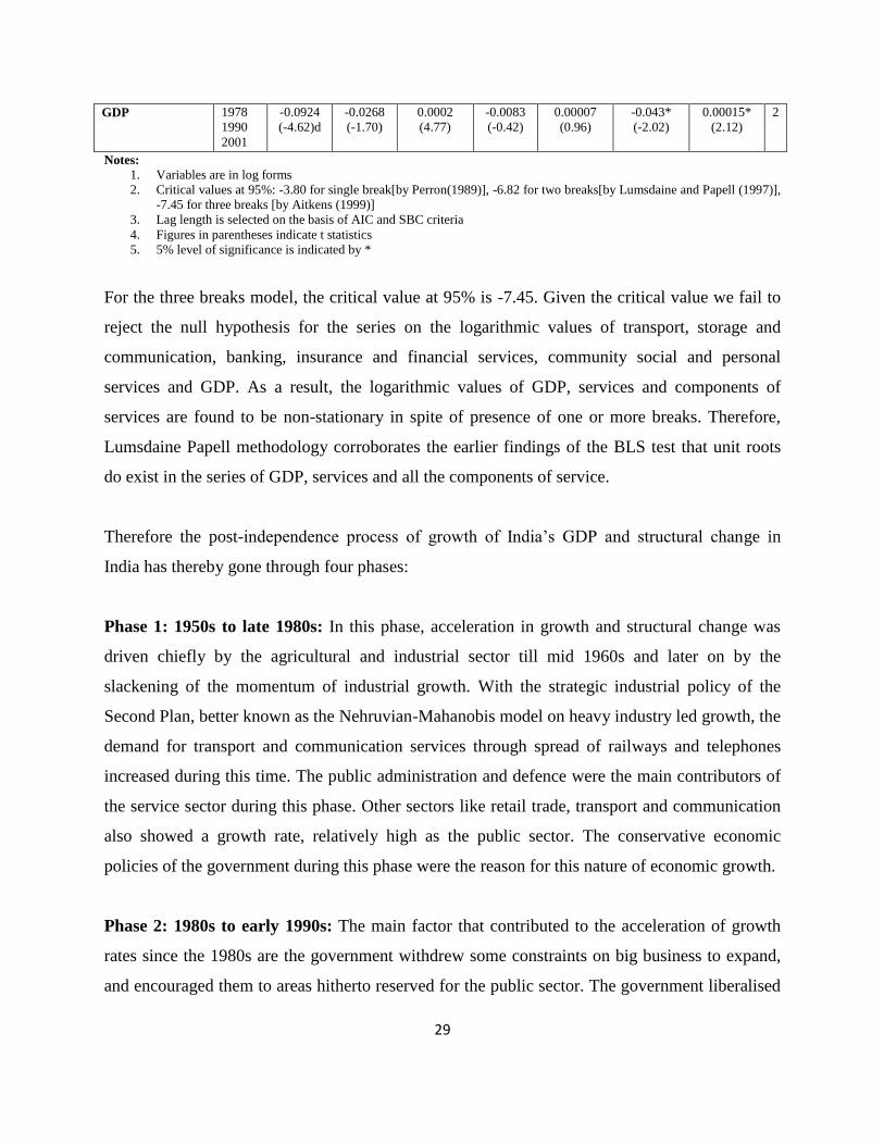
29

GDP 1978

1990

2001

-0.0924

(-4.62)d

-0.0268

(-1.70)

0.0002

(4.77)

-0.0083

(-0.42)

0.00007

(0.96)

-0.043*

(-2.02)

0.00015*

(2.12)

2

Notes:

1. Variables are in log forms

2. Critical values at 95%: -3.80 for single break[by Perron(1989)], -6.82 for two breaks[by Lumsdaine and Papell (1997)],

-7.45 for three breaks [by Aitkens (1999)]

3. Lag length is selected on the basis of AIC and SBC criteria

4. Figures in parentheses indicate t statistics

5. 5% level of significance is indicated by *

For the three breaks model, the critical value at 95% is -7.45. Given the critical value we fail to

reject the null hypothesis for the series on the logarithmic values of transport, storage and

communication, banking, insurance and financial services, community social and personal

services and GDP. As a result, the logarithmic values of GDP, services and components of

services are found to be non-stationary in spite of presence of one or more breaks. Therefore,

Lumsdaine Papell methodology corroborates the earlier findings of the BLS test that unit roots

do exist in the series of GDP, services and all the components of service.

Therefore the post-independence process of growth of India‟s GDP and structural change in

India has thereby gone through four phases:

Phase 1: 1950s to late 1980s: In this phase, acceleration in growth and structural change was

driven chiefly by the agricultural and industrial sector till mid 1960s and later on by the

slackening of the momentum of industrial growth. With the strategic industrial policy of the

Second Plan, better known as the Nehruvian-Mahanobis model on heavy industry led growth, the

demand for transport and communication services through spread of railways and telephones

increased during this time. The public administration and defence were the main contributors of

the service sector during this phase. Other sectors like retail trade, transport and communication

also showed a growth rate, relatively high as the public sector. The conservative economic

policies of the government during this phase were the reason for this nature of economic growth.

Phase 2: 1980s to early 1990s: The main factor that contributed to the acceleration of growth

rates since the 1980s are the government withdrew some constraints on big business to expand,

and encouraged them to areas hitherto reserved for the public sector. The government liberalised

30

credit for big borrowers, gave tax concession to large investors, and allowed the private sector to

borrow directly from the public. The shift towards a more service dominated pattern of growth

happened in this phase as a fallout of the government liberal policies. The rising share of public

sector was the main source of increasing share of services in GDP during this period. Among the

service sector components, community, social and personal services were those that developed

during this period in conjunction to the earlier phase.

Phase 3: 1990s to 2000: This phase brought about the private organized sector led crucial

strengthening of services dominated growth trajectory as a consequence to the earlier phase. This

may be due to the fallout of the economic reforms initiated in the early 1990s. The opening up of

the economy along with the increased investments, growing consumption and the outsourcing

boom boosted the growth of the software sector. The banking sector reforms of 1992 and 1995

formulated major policies in the financial sector as a part of the liberalisation process such as

providing licenses to private sector banks, opening of the insurance sector, etc. Real estate sector

development has been backed by both demand factors such as unfulfilled demand of dwelling

units and lack of infrastructure and supply side factors such as increased rationalisation of tax

structure, reduced borrowings cost and tax benefits to loan seekers, etc. The highest growth in

banking and finance met the demand for personal loans, thereby leading to real estate boom. The

car industry, like real estate developed during this period, with increased benefits to loan takers

and improved post purchase services. Again, with the liberation policies of the government, in a

regime of no control, manufacturing activity was taken over by China, as they produced goods

cheaper than home produced goods.

Early 2000 to 2010: This phase brought about an increase in GDP via infrastructure like

construction, transport, communication and business services in conjunction to the earlier phase.

With the innovations in transport storage and communications and financial services there has

been an upsurge in services GDP. The tourism industry that includes hotels and restaurants has

witnessed good times on account of increased passenger traffic (business and leisure). The

communication sector is one of the fastest growing sectors domestically. India‟s teledensity has

improved but it is still low as compared to other developing nations. India's mobile subscriber

31

base has increased manifold and low tariffs enhance higher usage to give a further impetus to

growth.

This periodisation of India‟s post-independence economic history therefore points towards the

importance of going beyond relating the dynamics of the Indian economy to the degree to which

the prevalent economic policy regime was restrictive or liberal in different periods. Therefore

India‟s economic growth is a long term story related to constraints embedded in her economic

structure, which neither the actual interventions nor liberalisation have been able to eliminate. It

is these constraints that need to be investigated towards proper understanding of the peculiarity

of Indian economic change.

These are some of the important explanation posed by the post-independence experience of

growth and structural change. The growth performance of India has moved from its earlier

version of State-led industrialisation in the public sector under an import-substituting regime to a

more globalised export-oriented framework with least interventions by the State and more

reliance on market-based allocations. The fact that this acceleration was not rooted in

industrialisation but rather a shift towards services only adds to the difficulties of policy shift

based explanations. This is especially because the initial service orientation of growth till the

1990s was related to an expanding public sector, while the post 1990s is actually the shift from

public sector to private sector driven growth of services, and the decisive shift of the private

organized sector towards services. Thus, the role of the private sector in growth becomes

prominent from the mid-1990s, but it only reinforced an already existing tendency towards

service dominated growth. Moreover, given the direct and indirect role of the public sector in the

development of many of the areas of rapid service growth, there may exist other deeper

continuities between the 1980s and later. All these, do suggest that economic policy was

important to the Indian story of economic change, whether the prevailing policy regime has been

restrictive or liberal.

Section V: Conclusion

In a nutshell, this paper focuses on the turning points of growth, suggesting that these growth

patterns were different resulting from the pattern of structural change in output in these periods.

32

This paper uses annual data of the components of GDP to determine endogenously the most

important years when structural breaks occurred and simultaneously test for the unit root

hypothesis in the presence of these breaks in GDP, services and subsector of services for the

Indian economy from 1950-51 to 2009-10. Based on the multiple structural breaks model of Bai

and Perron (1998, 2003), the post-independence Indian GDP growth structure has been broadly

defined into four regimes. The high GDP growth in the last two decades has been brought about

by the dominant components of the service sector mainly, transport, storage and communication

and banking, insurance and financial services. However, trade, hotel and restaurants in the last

decades have also high growth rate. It is only community, social and personal sector which has

shown a consistently low growth throughout decades. The subsequent unit root test by BLS

(1992) and Lumsdaine and Papell (1997) corroborates that fact in spite of the presence of

multiple structural breaks, all of these series are non-stationary at levels. The growth rates of the

sub-sector of services and GDP as a whole showed that the growth in the post globalisation era is

India has been massive as compared to the earlier regimes. However, the first break in services

came long back as compared to that of GDP and the second break in services actually occurred

almost a decade after the initiation of the economic reforms of the early 1990s. On the whole, the

break in service sector growth started much after the commencement of reforms, and therefore

may not be considered as an effect of liberalisation. But in case of fastest growing specialised

services like banking, insurance and financial services the structural break has more or less

matched with the break in GDP, establishing that this sector in particular had the positive fallout

of liberalisation in India.

The paper answers the basic research question to relating to services sector growth and its

structural transformation posed at the beginning of this paper. The structural transformation for

predominantly agrarian economy to a services orientation is therefore, seen first in 1978-79

followed by early 1990s. It is largely observed the service sector boom have grown manifold in

post globalisation India mainly due to the growth in banking, insurance, real estate, financial

services and transport, storage and communication. The banking sector reforms formulated

major policies in the financial sector like giving licenses to private sector banks as part of the

liberalisation process, opening of the insurance sector, etc. This growth is also attributed to the

33

liberalisation policy of the government, along with the increased investments, growing

consumption and the outsourcing boom boosted the growth of the software sector. The

communication sector is one of the fastest growing sectors domestically. India‟s teledensity has

improved but it is still low as compared to other developing nations. India's mobile subscriber

base has increased manifold and low tariffs enhance higher usage to give a further impetus to

growth. The intersectoral dynamics of the broad sectors of agriculture, industry and services

necessitates that services serve as an input in industrial sector in India. The demand for services

is not only driven by the manufacturing sector in India but also is absorbed largely by the

external sector. The gigantic amount of services exports is growth augmenting in the long run

for India. Therefore, services somewhat has played the role of engine of growth in the Indian

economy, specifically in post liberalisation era.

Bibliography

Ahluwalia, M. (2002). Economic Reforms in India Since 1991: Has Gradualism Worked.

Journal of Economic Perspectives, Vol. 16, No. 7 , 67-88.

Aitkins, F. J. (2002). “Multiple Structural break in the Nominal Interest Rate and Inflation in

Canada and the United States” . Preliminary Draft, Department of Economics, The University of

Alberta, Canada.

Andrews, D. (1993a). Tests for parameter instability and structural change with unknown change

point. Econometrica 61 , 821-856 (Corrigendum, 71, 395-397).

Andrews, D. (1993b). Exactly median-unbiasedestimation of first-order autoregressive/unit root

models. Econometrica 61 , 139-165.

Andrews, D. K., & Ploberger, W. (1994). Optimal tests when a nuisance parameter is present

only under the alternative. Econometrica 62 , 1383-1414.

Andrews, D. K., Lee, I., & Ploberger, W. (1996). Optimal change point tests for normal linear

regression. Journal of Econometrics 70 , 9-38.

Bai, J., & Perron, P. (2003). Computation and Analysis of Multiple Structural Change Models.

Journal of Applied Econometrics, Vol. 18, No. 1 .

Bai, J., & Perron, P. (1998). Estimating and Testing Linear Models with Multiple Structural

Changes. Econometrica, Vol 66, No.1 .

34

Balakrishnan, P. &.Permeshwaran, M. ( 2007a). Understanding growth regimes in India: Further

observations. Economic and Political Weekly .

Balakrishnan, P., & Permeshwaran, M. (2007). “Understanding growth regimes in India: A pre-

requisite”. Economic and Political Weekly, July 14th, .

Banerjee, A., Lumsdaine, R., & Stock, J. (1992). Recursive and sequential tests of the unit root

and trend break hypothesis: Theory and Interanational Evidence. Journal of Business and

Economic Statistics, 10 , 271-287.

Banga, R. (2005). “Critical issues in India‟s Services Led Growth. ICRIER Working Paper, 171,

October.

Banga, R. & Goldar, B. (2004). Contribution of Services to Output Growth Productivity in

Indian Manufacturing: Pre and Post Reform. ICRIER Working Paper, 139, August.

Basu, K. (2003). The Indian Economy: Up to 1991 and Since. BREAD Working Paper No 052,

December .

Baumol, W. J. (1986). Productivity growth, convergence, and welfare: what the long-run data

show? The American Economic Review , 1072-1085.

Baumol, W. (1967). Macroeconomics of Unbalanced Growth: an anatomy of Urban Crisis.

American Economic Review, 57 (3) , 415-426.

Ben_David, D., & Papell, D. H. (1995). The Great Wars, the Great Crash and the Unit Root

Hypothesis. Journal of Monetary Economics, Vol. 36 , pp. 453-475.

Ben-David, D., Lumdaine, R.,& Papell, D.H.(2003). Unit Root, Postwar Slowdowns and Long-

Run Growth: Evidence from Two Structural Breaks. Empirical Economics, 28(2) , pp. 303-319.

Bhagwati J, P. A. (2004). The muddles of Outsourcing. Journal of Economic Perspectives .

Bhagwati, J. N. (1984). Splintering and Disembodiment of Services and Developing Nations.

World Economy, June, 7(2), , 133-143.

Bhagwati, J. N. (1985). Why are Services Cheaper in the Poor Countries? In G. G. (ed.), Wealth

and Poverty, Essays in Development Economics Series (Vol. vol. 1, pp. 82-91). England:

Cambridge, MIT Press, Blackwell.

Bhattacharya, B. B., & Mitra, A. (1989). Agriculture Industry Growth Rates: Widening

Disparity: An Explanation. Economic and Political Weekly, August 26.

Bhattacharya, B. B., & Mitra, A. (1997). Changing Composition of Employment in Tertiary

Sector: A Cross-Country Analysis. Economic and Political Weekly, March 15 .

35

Bhattacharya, B. B., & Mitra, A. (1991). Excess Growth of the Tertiary Sector. Economic and

Political Weekly, June 1-8 .

Bhattacharya, B. B., & Mitra, A. (1990). Excess Growth of the Tertiary Sector: Issues and

Implications. Economic and Political Weekly .

Bhattacharya, B. B., & Sakthivel, S. (2004). Regional Growth and Disparity in India. Economic

and Political Weekly, March 6.

Boyce, J. (1987). Agrarian Impasse in Bengal: Institutional Constraints to Technological

Change. Oxford University Press.

Boyce, J. K. (1986). Kinked exponential models for growth rate estimation. Oxford Bulletin of

Economics and Statistics, 48 , 385-91 .

Christiano, L. (1992). Searching for a Break in GNP. Journal of Business and Economic

Statistics, 10 , pp. 237-249.

Clark, C. (1940, revised and reprinted in 1951). The Conditions of Economic Progress. London:

MacMillan & Co.Ltd.

CSO. (2011). National Accounts Statistics: Back Series 1950-51 to 2004-05. Central Statistical

Organisation, Ministry of Statistics and Programme Implementation.

Dasgupta, S., & Singh, A. (2005). Will Services be the New Engine of Economic Growth in

India? Working Paper No. 310 . Centre for Business Research, University of Cambridge.

Datta, M. (1999). Structural Break and Unit Root in Macroeconomic Time Series: Evidence from

a Developing Economy . Sankhya, The Indian Journal of Statistics, Series B, .

Datta, M. (1989). Tertiary Sector and Net Material Product: Indian Economy, 1950-51 to 1983-

84. Economic and Political Weekly, September 23. .

Datta, M. (2001). The Significance and Growth of the Tertiary Sector. Delhi: Northern Book

Centre.

De Long, B. (2003). India Since Independence: An Analytic Growth Narrative. In D. R. (ed.), In

Search of Prosperity: Analytic Narratives on Economic Growth. New Jersey: Princeton

University Press, Princeton.

Dholakia, R. H. (1994). Spatial Dimension of Acceleration of Economic Growth in India.

Economic and Political Weekly, Vol 29, No 35 .

Dholakia, R. H. (2007). Understanding growth regimes in India: Some observations. Economic

and Political Weekly, August 25th .

36

Dholakia, R., & Sapre, A. (2011). Estimating structural breaks endogenously in India‟s post-

independence growth path: An Empirical Critique. Journal of Quantitative Economics, Vol. 9

No. (2) .

Dickey, D. A., & Fuller, W. A. (1979). Distribution of the Estimators for Autoregressive Time

Series With a Unit Root. Journal of the American Statistical Association,7 4, , 427-431.

Dickey, D. A., & Fuller, W. A. (1981). Likelihood Ratio Statistics for Autoregressive Time

Series With a Unit Root. Econometrica, 49 , 1057-1072.

Economic Survey, (2011): Government of India

Eichengreen, B., & Gupta, P. (2010). The Service Sector as India„s Road to Economic Growth.

Indian Council of Research on International Economic Relations, New Delhi. , ICRIER Working

Paper Series, Number 249.

Eichengreen, B., & Gupta, P. (2009). The Two Waves of Service Sector Growth. National

Bureau of Economic Resaerch, Cambridge, Masssachusetts , NBER Working Paper Series,

Working Paper Number 14968.

Elfring, T. (1989). New Evidence on the Expansion of Service Employment in Advanced

Economies . Review of Income and Wealth, Series 35, No.4. .

Fisher, A. G. (1952). A Note on Tertiary Production . The Economic Journal, Vol. 62, No. 248 .

Gordon, J., & Gupta, P. (2004). Understanding India‟s Services Revolution. IMF Working Paper

WP/04/171, September.

Griliches, Z. (1992). Output Measurement in the Service Sectors, . In Z. Griliches (ed), ,NBER

Studies in Income and Wealth (Vol. Vol. 56). Chicago: University of Chicago Press.

Grubel, H. G. (1987). All Traded Services are Embodied in Materials or People. The World

Economy, 10 (3), 319–330.

Hansda, S. (2002). Services in the Indian Economy: A Staff Report. RBI Staff Studies,

September, Mumbai. .

Hansda, S. (2001). Sustainability of Services led growth: An input- output Analysis of the Indian

Economy. RBI Occasional Working Paper, Vol 22, No.1, 2 and 3. .

Hatekar, N., & Dongre, A. (2005). Structural Breaks in India„s Growth: Revisiting the Debate

with a Longer Perspective. Economic and Political Weekly, Vol.40, No. 14, April 2.

Joshi, S. (2004). Tertiary sector driven growth in India: Impact on Employment and Poverty.

Economic and Political Weekly .

37

Kaldor, N. (1950). A contribution to the theory of the trade cycle. Oxford: Oxford University

Press.

Kaldor, N. (1957). A Model of Economic Growth. The Economic Journal, Vol. 67(268), 591–

624.

Kaldor, N. (1966). Causes of the Slow Rate of Economic Growth of the United Kingdom.

Cambridge: Cambridge University Press.

Kaldor, N. (1967). Strategic Factors in Economic Development. Cornell University, Ithaca.

Kaldor, N. (1975). What is wrong with economic theory. Quarterly Journal of Economics, 89 ,

347–357 .

Kochar, K., Kumar, U., Rajan, R., Subramaniam, A., & Tokatlidis, I. (2006). India‟s Pattern of

Development: What Happened, What Follows?,. IMF Working Paper WP/06/22.

Kuznets, S. (1966). Modern Economic Growth . New Haven: Yale UniversityPress.

Kuznets, S. (1973). Modern economic growth: findings and reflections. American Economic

Review 63 , 247–258.

Kuznets, S. (1972). Modern Economic Growth: Rate, Structure, and Spread. New Delhi: Indian

Edition,Oxford and IBH Publishing Co. Pvt. Ltd.

Lumsdaine, R., & Papell, D. (1997). Multiple trend breaks and the unit root hypothesis. Review

of Economics and Statistics, 79 , 212-218.

Mazumdar, S (2010). Industry and services in growth and structural change in India: Some

unexplored features. ISID, MPRA Paper No. 20401

Mitra, A. (1988). Disproportionality and the Services Sector: A Note. Social Scientist .

Nagaraj, R. (2006). Aspects of India’s Economic Growth and Reforms. New Delhi: Academic

Foundation .

Nagaraj, R. (2009). Is Services Sector Output Overestimated? An Inquiry. Economic and

Political Weekly, Vol. 44, No. 5, January 31 .

Nagraj, R. (1990). Growth Rate of India s GDP, 1950-51 to 1987-88-Examination of Alternative

Hypotheses. Economic and Political Weekly, Vol. 25, No. 26 .

Nagraj, R. (1991). Increase in India‟s growth rate: Discussion. Economic and Political Weekly,

Vol. 27, No. 15 .

38

Nelson, C. R., & Plosser, C. I. (1982). Trends and Random Walks in Macroeconomic Time

Series. Journal of Monetary Economics, 10, , 139-162.

Ng, S., & Perron, P. (1995). Unit root tests in ARMA models with data dependent methods for

the selection of the truncation lag. Journal of American Statistical Association, 90 , 268-281.

Ohara, H. (1999). A unit root test with multiple trend breaks: A theory and application to US and

Japanese macroeconomic time series. The Japanese Economic Review, Vol. 50 , pp. 266-290.

Panagariya, A. (2004). Growth and Reforms during 1980s and 1990s. Economic and Political

Weekly, June 19: 2581-94 .

Panchmukhi, V. R., Nambiar, & Meheta, R. (1986). Structural Change and Economic Growth in

Developing Countries. VIII World Economic Congress of the International Economic

Association, Theme 4, December .

Pappel, D. Lumsdaine, R., & Papell, D.H (2003). The uncertain unit root in US real GDP:

Evidence with restricted and unrestricted structural change. Journal of Money Credit and

Banking, Vol. 36 , pp. 423-427.

Perron, P., &Vogelsang, T. J.. (1992). Nonstationarity and Level Shifts with an Application to

Purchasing Power Parity. Journal of Business and Economic Statistics, 10 , pp. 301–320.

Perron, P. (1997). Further Evidence on Breaking Trend Functions in Macroeconomic Variables.

Journal of Econometrics, 80 (2) , pp.355-385.

Perron, P. (1989). The Great Crash, the Oil Price Shock and the Unit Root Hypothesis.

Econometrica, 57 , 1361-1401.

Perron, P. (1994). Trend, Unit Root Hypothesis and Structural Change in Macroeconomic Time

Series. In B. Roa, Cointegration for Applied Economists. St. Martin‟s Press.

Pesaran, M. H., Shin, Y., & Smith, R. J. (2001). “Bounds testing approaches to the analysis of

level relationship.”. Journal of Applied Economics 16: 289-326.

Phillips, P.(1988). Multiple Regression With Integrated Time Series. Contemporary

Mathematics, 80, , 79-105.

Phillips, P. (1987). Time Series Regression With a Unit Root. Econometrica, 55, , 277-301.

Phillips, P., & Perron, P. (1988). Testing for a Unit Root in Time Series Regression. Biometrica

75(2) , pp. 335-346.

Rakshit, M. (2007). Services-led Growth:The Indian Experience. ICRA Bulletin, Money and

Finance .

39

Rodrik, D., & Subramanian, A. (2004). From Hindu Growth to Productivity Surge: The Mystery

of the Indian Growth Transition. National Bureau of Economic Research Paper No 10376.

Saith, A. (2006). From Universal Values to Millennium Development Goals: Lost in Translation.

Development and Change, 37 (6), 1167-1199.

Sarkar, S., & Mehta, B. S. (2006). Employment profile of ICT Sector. Paper presented at the

seminar on Knowledge based industries, Employment and Global Competitiveness, forum for

Global Knowledge Sharing .

Sastry, D., Singh, B., Bhattacharya, K., & Unnikrishnan, N. (2003). Sectoral linkages and

Growth Prospects: Reflections on the Indian Economy. Economic and Political Weekly 38, June

14, , 2390-2397.

Singh, N. (2006). Services Led Industrialisation in India: Assessment and Lessons. UCGC,

MPRA Paper No. 1446 .

Sinha, A., & Tejani, S. (2004). Trend Break in India‟s GDP Growth Rate: Some Comments.

Economic and Political Weekly, 39 (52), 5634-5639.

Soubbotina, T. P. (2004). Beyond economic growth: an introduction to sustainable development.

Wasington, D.C: World Bank.

Srinivasan, T. (2003). Indian Economy: Current Problems and Future Prospects. Working Paper

No. 173, Stanford Centre for International Development .

Verma, R. (2006). India‟s Service Sector Growth: A “New” Revolution. DEGIT Conference

Paper .

Wallack, J. S. (2004). Structural Breaks in Indian Macroeconomic Data. Economic and Political

Weekly, October 11: 4312-15 .

World Bank. (2004). Sustaining India’s Services Revolution: Access to Foreign Markets,

Domestic Reform and International Negotiations. South Asia Region: India.

World Bank. (1995). India: Recent Economic Developments and Prospects. Washington D.C.

Wu, Y. (2004). Service Sector Growth in China and India: A Comparison. School of Economics

and Commerce, University of Western Australia, Economics Discussion/Working Paper 07-04.

Zivot, E., & Andrews, D. (1992). Further evidence of great crash, the oil price shock and unit

root hypothesis. Journal of Business and Economic Statistics, 10, , 251-270.