tensor algebra - oafak.comoafak.com/wp-content/uploads/2013/01/2-tensor-algebra-jan-2013.pdftensor...

Tensor Algebra Tensors as Linear Mappings

A second Order Tensor 𝑻 is a linear mapping from a vector space to itself. Given 𝒖 ∈ V the mapping,

𝑻: V → V

states that ∃ 𝒘 ∈ V such that, 𝑻 𝒖 = 𝒘.

Every other definition of a second order tensor can be derived from this simple definition. The tensor character of an object can be established by observing its action on a vector.

Second Order Tensor

[email protected] 12/30/2012 Department of Systems Engineering, University of Lagos 2

The mapping is linear. This means that if we have two runs of the process, we first input 𝒖 and later input 𝐯. The outcomes 𝑻(𝒖) and 𝑻(𝐯), added would have been the same as if we had added the inputs 𝒖 and 𝐯 first and supplied the sum of the vectors as input. More compactly, this means,

𝑻 𝒖 + 𝐯 = 𝑻(𝒖) + 𝑻(𝐯)

Linearity


Linearity further means that, for any scalar 𝛼 and tensor 𝑻 𝑻 𝛼𝒖 = 𝛼𝑻 𝒖

The two properties can be added so that, given 𝛼, 𝛽 ∈ R, and 𝒖, 𝐯 ∈ V, then

𝑻 𝛼𝒖 + 𝛽𝐯 = 𝛼𝑻 𝒖 + 𝛽𝑻 𝐯

Since we can think of a tensor as a process that takes an input and produces an output, two tensors are equal only if they produce the same outputs when supplied with the same input. The sum of two tensors is the tensor that will give an output which will be the sum of the outputs of the two tensors when each is given that input.

Linearity


In general, 𝛼, 𝛽 ∈R , 𝒖, 𝐯 ∈ V and 𝑺, 𝑻 ∈ T 𝛼𝑺𝒖 + 𝛽𝑻𝒖 = (𝛼𝑺 + 𝛽𝑻)𝒖

With the definition above, the set of tensors constitute a vector space with its rules of addition and multiplication by a scalar. It will become obvious later that it also constitutes a Euclidean vector space with its own rule of the inner product.

Vector Space


Notation.

It is customary to write the tensor mapping without the parentheses. Hence, we can write,

𝑻𝒖 ≡ 𝑻(𝒖)

For the mapping by the tensor 𝑻 on the vector variable and dispense with the parentheses unless when needed.

Special Tensors


The annihilator 𝑶 is defined as the tensor that maps all vectors to the zero vector, 𝒐:

𝑶𝑢 = 𝒐, ∀𝒖 ∈ V

Zero Tensor or Annihilator


The identity tensor 𝟏 is the tensor that leaves every vector unaltered. ∀𝒖 ∈ V ,

𝟏𝒖 = 𝒖

Furthermore, ∀𝛼 ∈ R , the tensor, 𝛼𝟏 is called a spherical tensor.

The identity tensor induces the concept of an inverse of a tensor. Given the fact that if 𝑻 ∈ T and 𝒖 ∈ V , the mapping 𝒘 ≡ 𝑻𝒖 produces a vector.

The Identity


Consider a linear mapping that, operating on 𝒘, produces our original argument, 𝒖, if we can find it:

𝒀𝒘 = 𝒖

As a linear mapping, operating on a vector, clearly, 𝒀 is a tensor. It is called the inverse of 𝑻 because,

𝒀𝒘 = 𝒀𝑻𝒖 = 𝒖

So that the composition 𝒀𝑻 = 𝟏, the identity mapping. For this reason, we write,

𝒀 = 𝑻−1

The Inverse


It is easy to show that if 𝒀𝑻 = 𝟏, then 𝑻𝒀 = 𝒀𝑻 = 𝟏.

HW: Show this.

The set of invertible sets is closed under composition. It is also closed under inversion. It forms a group with the identity tensor as the group’s neutral element

Inverse


Given 𝒘, 𝐯 ∈ V , The tensor 𝑨T satisfying

𝒘 ⋅ 𝑨T𝐯 = 𝐯 ⋅ (𝑨𝒘)

Is called the transpose of 𝐴.

A tensor indistinguishable from its transpose is said to be symmetric.

Transposition of Tensors


There are certain mappings from the space of tensors to the real space. Such mappings are called Invariants of the Tensor. Three of these, called Principal invariants play key roles in the application of tensors to continuum mechanics. We shall define them shortly.

The definition given here is free of any association with a coordinate system. It is a good practice to derive any other definitions from these fundamental ones:

Invariants


If we write 𝐚, 𝐛, 𝐜 ≡ 𝐚 ⋅ 𝐛 × 𝐜

where 𝐚, 𝐛, and 𝐜 are arbitrary vectors.

For any second order tensor 𝑻, and linearly independent 𝐚, 𝐛, and 𝐜, the linear mapping 𝐼1: T →R

𝐼1 𝑻 ≡ tr 𝑻 =𝑻𝐚, 𝐛, 𝐜 + 𝐚, 𝑻𝐛, 𝐜 + [𝐚, 𝐛, 𝑻𝐜]

[𝐚, 𝐛, 𝐜]

Is independent of the choice of the basis vectors 𝐚, 𝐛, and 𝐜. It is called the First Principal Invariant of 𝑻 or Trace of 𝑻 ≡ tr 𝑻 ≡ 𝐼1(𝑻)

The Trace


The trace is a linear mapping. It is easily shown that 𝛼, 𝛽 ∈ R , and 𝑺, 𝑻 ∈ T

tr 𝛼𝑺 + 𝛽𝑻 = 𝛼tr 𝑺 + 𝛽tr(𝑻)

HW. Show this by appealing to the linearity of the vector space.

While the trace of a tensor is linear, the other two principal invariants are nonlinear. WE now proceed to define them

The Trace


The second principal invariant 𝐼2 𝑺 is related to the trace. In fact, you may come across books that define it so. However, the most common definition is that

𝐼2 𝑺 =1

2𝐼12 𝑺 − 𝐼1(𝑺

2)

Independently of the trace, we can also define the second principal invariant as,

Square of the trace


The Second Principal Invariant, 𝐼2 𝑻 , using the same notation as above is 𝑻𝒂 , 𝑻𝒃 , 𝒄 + 𝒂, 𝑻𝒃 , 𝑻𝒄 + 𝑻𝒂 , 𝒃, 𝑻𝒄

𝒂, 𝒃, 𝒄

=1

2tr2 𝑻 − tr 𝑻2

that is half the square of trace minus the trace of the square of 𝑻 which is the second principal invariant.

This quantity remains unchanged for any arbitrary selection of basis vectors 𝒂, 𝒃 and 𝒄.

Second Principal Invariant


The third mapping from tensors to the real space underlying the tensor is the determinant of the tensor. While you may be familiar with that operation and can easily extract a determinant from a matrix, it is important to understand the definition for a tensor that is independent of the component expression. The latter remains relevant even when we have not expressed the tensor in terms of its components in a particular coordinate system.

The Determinant


As before, For any second order tensor 𝑻, and any linearly independent vectors 𝐚, 𝐛, and 𝐜,

The determinant of the tensor 𝑻,

det 𝑻 =𝑻𝒂 , 𝑻𝒃 , 𝑻𝒄

𝒂, 𝒃, 𝒄

(In the special case when the basis vectors are orthonormal, the denominator is unity)

The Determinant


It is good to note that there are other principal invariants that can be defined. The ones we defined here are the ones you are most likely to find in other texts.

An invariant is a scalar derived from a tensor that remains unchanged in any coordinate system. Mathematically, it is a mapping from the tensor space to the real space. Or simply a scalar valued function of the tensor.

Other Principal Invariants


The trace provides a simple way to define the inner product of two second-order tensors. Given 𝑺, 𝑻 ∈ T

The trace, tr 𝑺𝑇𝑻 = tr(𝑺𝑻𝑇)

Is a scalar, independent of the coordinate system chosen to represent the tensors. This is defined as the inner or scalar product of the tensors 𝑺 and 𝑻. That is,

𝑺: 𝑻 ≡ tr 𝑺𝑇𝑻 = tr(𝑺𝑻𝑇)

Inner Product of Tensors


The trace automatically induces the concept of the norm of a vector (This is not the determinant! Note!!) The square root of the scalar product of a tensor with itself is the norm, magnitude or length of the tensor:

𝑻 = tr(𝑻𝑇𝑻) = 𝑻: 𝑻

Attributes of a Euclidean Space


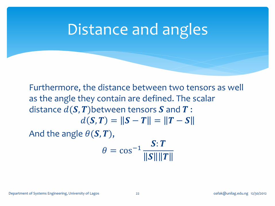
Furthermore, the distance between two tensors as well as the angle they contain are defined. The scalar distance 𝑑(𝑺, 𝑻)between tensors 𝑺 and 𝑻 :

𝑑 𝑺, 𝑻 = 𝑺 − 𝑻 = 𝑻 − 𝑺

And the angle 𝜃(𝑺, 𝑻),

𝜃 = cos−1𝑺: 𝑻

𝑺 𝑻

Distance and angles


A product mapping from two vector spaces to T is defined as the tensor product. It has the following properties:

"⊗":V ×V → T 𝒖⊗ 𝒗 𝒘 = (𝒗 ⋅ 𝒘)𝒖

It is an ordered pair of vectors. It acts on any other vector by creating a new vector in the direction of its first vector as shown above. This product of two vectors is called a tensor product or a simple dyad.

The Tensor Product


It is very easily shown that the transposition of dyad is simply a reversal of its order. (HW. Show this).

The tensor product is linear in its two factors.

Based on the obvious fact that for any tensor 𝑻 and 𝒖, 𝒗,𝒘 ∈ V , 𝑻 𝒖⊗ 𝒗 𝒘 = 𝑻𝒖 𝒗 ⋅ 𝒘 = 𝑻𝒖 ⊗ 𝒗 𝒘

It is clear that 𝑻 𝒖⊗ 𝒗 = 𝑻𝒖 ⊗ 𝒗

Show this neatly by operating either side on a vector

Furthermore, the contraction, 𝒖⊗ 𝒗 𝑻 = 𝒖⊗ 𝑻𝑇𝒗

A fact that can be established by operating each side on the same vector.

Dyad Properties


Recall that for 𝒘, 𝐯 ∈ V , The tensor 𝑨T satisfying

𝒘 ⋅ 𝑨T𝐯 = 𝐯 ⋅ (𝑨𝒘)

Is called the transpose of 𝑨. Now let 𝑨 = 𝒂⊗ 𝒃 a dyad. 𝐯 ⋅ 𝑨𝒘 =

= 𝐯 ⋅ 𝒂⊗ 𝒃 𝒘 = 𝐯 ⋅ 𝒂 𝒃 ⋅ 𝒘 = 𝐯 ⋅ 𝒂 𝒃 ⋅ 𝒘 = 𝒘 ⋅ 𝒃 𝐯 ⋅ 𝒂 = 𝒘 ⋅ 𝒃⊗ 𝒂 𝐯

So that 𝒂⊗ 𝒃 T = 𝒃⊗ 𝒂

Showing that the transpose of a dyad is simply a reversal of its factors.

Transpose of a Dyad


If 𝐧 is the unit normal to a given plane, show that the tensor 𝐓 ≡ 𝟏 − 𝐧⊗ 𝐧 is such that 𝐓𝐮 is the projection of the vector 𝐮 to the plane in question.

Consider the fact that 𝐓 ⋅ 𝐮 = 𝟏𝐮 − 𝐧 ⋅ 𝐮 𝐧 = 𝐮 − 𝐧 ⋅ 𝐮 𝐧

The above vector equation shows that 𝐓𝐮 is what remains after we have subtracted the projection 𝐧 ⋅ 𝐮 𝐧 onto the normal. Obviously, this is the

projection to the plane itself. 𝐓 as we shall see later is called a tensor projector.


Consider a contravariant vector component 𝑎𝑘 let us take a product of this with the Kronecker Delta:

𝛿𝑗𝑖𝑎𝑘

which gives us a third-order object. Let us now perform a contraction across (by taking the superscript index from 𝐴𝑘

and the subscript from 𝛿𝑗𝑖) to arrive at,

𝑑𝑖 = 𝛿𝑗𝑖𝑎𝑗

Observe that the only free index remaining is the superscript 𝑖 as the other indices have been contracted (it is consequently a summation index) out in the implied summation. Let us now expand the RHS above, we find,

Substitution Operation


𝑑𝑖 = 𝛿𝑗𝑖𝑎𝑗 = 𝛿1

𝑖𝑎1 + 𝛿2𝑖𝑎2 + 𝛿3

𝑖𝑎3

Note the following cases:

if 𝑖 = 1, we have 𝑑1 = 𝑎1, if 𝑖 = 2, we have 𝑑2 = 𝑎2 if 𝑖 = 3, we have 𝑑3 = 𝑎3. This leads us to conclude

therefore that the contraction, 𝛿𝑗𝑖𝑎𝑗 = 𝑎𝑖. Indicating

that that the Kronecker Delta, in a contraction, merely substitutes its own other symbol for the symbol on the vector 𝑎𝑗 it was contracted with. This fact, that the Kronecker Delta does this in general earned it the alias of “Substitution Operator”.

Substitution


Operate on the vector 𝒛 and let 𝑻𝒛 = 𝒘. On the LHS, 𝒖⊗ 𝒗 𝑻𝒛 = 𝒖⊗ 𝒗 𝒘

On the RHS, we have:

𝒖⊗ 𝑻𝑇𝒗 𝒛 = 𝒖 𝑻𝑇𝒗 ⋅ 𝒛 = 𝒖 𝒛 ⋅ 𝑻𝑇𝒗

Since the contents of both sides of the dot are vectors and dot product of vectors is commutative. Clearly,

𝒖⊗ 𝒛 ⋅ 𝑻𝑇𝒗 = 𝒖⊗ 𝒗 ⋅ 𝑻𝒛

follows from the definition of transposition. Hence,

𝒖⊗ 𝑻𝑇𝒗 𝒛 = 𝒖 𝒗 ⋅ 𝒘 = 𝒖⊗ 𝒗 𝒘

Composition with Tensors


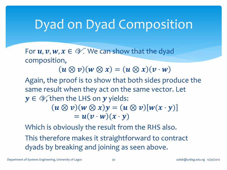
For 𝒖, 𝒗,𝒘, 𝒙 ∈ V , We can show that the dyad composition,

𝒖⊗ 𝒗 𝒘⊗ 𝒙 = 𝒖⊗ 𝒙 𝒗 ⋅ 𝒘

Again, the proof is to show that both sides produce the same result when they act on the same vector. Let 𝒚 ∈ V , then the LHS on 𝒚 yields:

𝒖⊗ 𝒗 𝒘⊗ 𝒙 𝒚 = 𝒖⊗ 𝒗 𝒘(𝒙 ⋅ 𝒚)= 𝒖 𝒗 ⋅ 𝒘 (𝒙 ⋅ 𝒚)

Which is obviously the result from the RHS also.

This therefore makes it straightforward to contract dyads by breaking and joining as seen above.

Dyad on Dyad Composition


Show that the trace of the tensor product 𝐮⊗ 𝐯 is 𝐮 ⋅𝐯.

Given any three independent vectors 𝐚, 𝐛, and 𝐜, (No loss of generality in letting the three independent vectors be the curvilinear basis vectors 𝐠1, 𝐠2 and 𝐠3). Using the above definition of trace, we can write that,

Trace of a Dyad


tr 𝐮⊗ 𝐯

=𝐮⊗ 𝐯 𝐠1 , 𝐠2, 𝐠3 + 𝐠1, 𝐮 ⊗ 𝐯 𝐠2 , 𝐠3 + 𝐠1, 𝐠2, 𝐮 ⊗ 𝐯 𝐠3

𝐠1, 𝐠2, 𝐠3

=1

𝜖123𝑣1𝐮, 𝐠2, 𝐠3 + 𝐠1, 𝑣2𝐮, 𝐠3 + 𝐠1, 𝐠2, 𝑣3𝐮

=1

𝜖123𝑣1𝐮 ⋅ 𝜖23𝑖𝐠

𝑖 + 𝜖31𝑖𝐠𝑖 ⋅ 𝑣2𝐮 + 𝜖12𝑖𝐠

𝑖 ⋅ 𝑣3𝐮

=1

𝜖123𝑣1𝐮 ⋅ 𝜖231𝐠

1 + 𝜖312𝐠2 ⋅ 𝑣2𝐮 + 𝜖123𝐠

3 ⋅ 𝑣3𝐮

= 𝑣𝑖𝑢𝑖 = 𝐮 ⋅ 𝐯

Trace of a Dyad


It is easy to show that for a tensor product 𝑫 = 𝒖⊗ 𝒗 ∀𝒖, 𝒗 ∈ V 𝑰2 𝑫 = 𝑰3 𝑫 = 0

HW. Show that this is so.

We proved earlier that 𝑰1 𝑫 = 𝒖 ⋅ 𝒗

Furthermore, if 𝑻 ∈ T , then, tr 𝑻𝒖⊗ 𝒗 = tr 𝒘⊗ 𝒗 = 𝒘 ⋅ 𝒗 = 𝑻𝒖 ⋅ 𝒗

Other Invariants of a Dyad


Given 𝑻 ∈ T , for any basis vectors 𝐠𝑖 ∈ V , 𝑖 = 1,2,3 𝑻𝑗 ≡ 𝑻𝐠𝑗 ∈ V , 𝑗 = 1,2,3

by the law of tensor mapping. We proceed to find the components of 𝑻𝑗 on this same basis. Its covariant

components, just like in any other vector are the scalars, 𝑻𝛼 𝑗 = 𝐠𝛼 ⋅ 𝑻𝑗

Specifically, these components are 𝑻1 𝑗 , 𝑻2 𝑗 , 𝑻3 𝑗

Tensor Bases & Component Representation


We can dispense with the parentheses and write that 𝑇𝛼𝑗 ≡ 𝑇𝛼 𝑗 = 𝑻𝑗 ⋅ 𝐠𝛼

So that the vector 𝑻𝐠𝑗 = 𝑻𝑗 = 𝑇𝛼𝑗𝐠

𝛼

The components 𝑇𝑖𝑗 can be found by taking the dot

product of the above equation with 𝐠𝑖:

𝐠𝑖 ⋅ 𝑻𝐠𝑗 = 𝑇𝛼𝑗 𝐠𝑖 ⋅ 𝐠𝛼 = 𝑇𝑖𝑗

𝑇𝑖𝑗 = 𝐠𝑖 ⋅ 𝑻𝐠𝑗

= tr 𝑻𝐠𝑗⊗𝐠𝑖 = 𝑻: 𝐠𝑖⊗𝐠𝑗

Tensor Components


The component 𝑇𝑖𝑗 is simply the result of the inner

product of the tensor 𝑻 on the tensor product 𝐠𝑖⊗𝐠𝑗.

These are the components of 𝑻 on the product dual of this particular product base.

This is a general result and applies to all product bases:

It is straightforward to prove the results on the following table:

Tensor Components


Components of 𝑻 Derivation Full Representation

𝑇𝑖𝑗 𝑻: (𝐠𝑖⊗𝐠𝑗) 𝑻 = 𝑇𝑖𝑗𝐠𝑖⊗𝐠𝑗

𝑇𝑖𝑗 𝑻: 𝐠𝑖⊗𝐠𝑗 𝑻 = 𝑇𝑖𝑗𝐠𝑖⊗𝐠𝑗

𝑇𝑖.𝑗

𝑻: (𝐠𝑖⊗𝐠𝑗) 𝑻 = 𝑇𝑖

.𝑗𝐠𝑖⊗𝐠𝑗

𝑇.𝑖𝑗 𝑻: (𝐠𝑗⊗𝐠𝑖) 𝑻 = 𝑇.𝑖

𝑗𝐠𝑗⊗𝐠

𝑖

Tensor Components


Components of 𝟏 Derivation Full Representation

𝟏 𝑖𝑗 = 𝑔𝑖𝑗 𝟏: (𝐠𝑖⊗𝐠𝑗) 𝟏 = 𝑔𝑖𝑗𝐠𝑖⊗𝐠𝑗

𝟏 𝑖𝑗 = 𝑔𝑖𝑗 𝟏: 𝐠𝑖⊗𝐠𝑗 𝟏 = 𝑔𝑖𝑗𝐠𝑖⊗𝐠𝑗

𝟏 𝑖.𝑗= 𝛿𝑖.𝑗

𝟏: (𝐠𝑖⊗𝐠𝑗) 𝟏 = 𝛿𝑖

.𝑗𝐠𝑖⊗𝐠𝑗 = 𝐠

𝑖⊗𝐠𝑖

𝟏 .𝑖𝑗= 𝛿 .𝑖𝑗

𝟏: (𝐠𝑗⊗𝐠𝑖) 𝟏 = 𝛿.𝑖𝑗𝐠𝑗⊗𝐠

𝑖 = 𝐠𝑗⊗𝐠𝑗

IdentityTensor Components

It is easily verified from the definition of the identity tensor and the inner product that: (HW Verify this)

Showing that the Kronecker deltas are the components of the identity tensor in certain (not all) coordinate bases.


The above table shows the interesting relationship between the metric components and Kronecker deltas.

Obviously, they are the same tensors under different bases vectors.

Kronecker and Metric Tensors


It is easy to show that the above tables of component representations are valid. For any 𝐯 ∈ V , and 𝑻 ∈ T,

𝑻 − 𝑇𝑖𝑗𝐠𝑖⊗𝐠𝑗 𝐯 = 𝑻𝐯 − 𝑇𝑖𝑗 𝐠

𝑖⊗𝐠𝑗 𝐯

Expanding the vector in contravariant components, we have,

𝑻𝐯 − 𝑇𝑖𝑗 𝐠𝑖⊗𝐠𝑗 𝐯 = 𝑻𝑣𝛼𝐠𝛼 − 𝑇𝑖𝑗 𝐠

𝑖⊗𝐠𝑗 𝑣𝛼𝐠𝛼

= 𝑻𝑣𝛼𝐠𝛼 − 𝑇𝑖𝑗𝑣𝛼𝐠𝑖 𝐠𝑗 ⋅ 𝐠𝛼

= 𝑻𝑣𝛼𝐠𝛼 − 𝑇𝑖𝑗𝑣𝛼𝐠𝑖𝛿𝛼

𝑗

= 𝑻𝛼 𝑣𝛼 − 𝑇𝑖𝑗𝑣

𝑗𝐠𝑖 = 𝑻𝛼 𝑣𝛼 − 𝑻𝑗𝑣

𝑗

= 𝒐

∴ 𝑻 = 𝑇𝑖𝑗𝐠𝑖⊗𝐠𝑗

Component Representation


The transpose of 𝑻 = 𝑇𝑖𝑗𝐠𝑖⊗𝐠𝑗 is 𝑻𝑇 = 𝑇𝑖𝑗𝐠

𝑗⊗𝐠𝑖.

If 𝑻 is symmetric, then,

𝑇𝑖𝑗𝐠𝑖⊗𝐠𝑗 = 𝑇𝑖𝑗𝐠

𝑗⊗𝐠𝑖 = 𝑇𝑗𝑖𝐠𝑖⊗𝐠𝑗

Clearly, in this case, 𝑇𝑖𝑗 = 𝑇𝑗𝑖

It is straightforward to establish the same for contravariant components. This result is impossible to establish for mixed tensor components:

Symmetry


For mixed tensor components,

𝑻 = 𝑇𝑖.𝑗𝐠𝑖⊗𝐠𝑗

The transpose,

𝑻T = 𝑇𝑖.𝑗𝐠𝑗⊗𝐠

𝑖= 𝑇𝑗.𝑖𝐠𝑖⊗𝐠

𝑗

While symmetry implies that,

𝑻 = 𝑇𝑖.𝑗𝐠𝑖⊗𝐠𝑗 = 𝑻

T = 𝑇𝑗.𝑖𝐠𝑖⊗𝐠

𝑗

We are not able to exploit the dummy variables to bring the two sides to a common product basis. Hence the symmetry is not expressible in terms of their components.

Symmetry


A tensor is antisymmetric if its transpose is its negative. In product bases that are either covariant or contravariant, antisymmetry, like symmetry can be expressed in terms of the components:

The transpose of 𝑻 = 𝑇𝑖𝑗𝐠𝑖⊗𝐠𝑗 is 𝑻𝑇 = 𝑇𝑖𝑗𝐠

𝑗⊗𝐠𝑖.

If 𝑻 is antisymmetric, then,

𝑇𝑖𝑗𝐠𝑖⊗𝐠𝑗 = −𝑇𝑖𝑗𝐠

𝑗⊗𝐠𝑖 = −𝑇𝑗𝑖𝐠𝑖⊗𝐠𝑗

Clearly, in this case, 𝑇𝑖𝑗 = −𝑇𝑗𝑖

It is straightforward to establish the same for contravariant components. Antisymmetric tensors are also said to be skew-symmetric.

AntiSymmetry


For any tensor 𝐓, define the symmetric and skew parts

sym 𝐓 ≡1

2𝐓 + 𝐓T , and skw 𝐓 ≡

1

2𝐓 − 𝐓T . It is easy

to show the following: 𝐓 = sym 𝐓 + skw 𝐓

skw sym 𝐓 = sym skw 𝐓 = 0

We can also write that,

sym 𝐓 =1

2𝑇𝑖𝑗 + 𝑇𝑗𝑖 𝐠

𝑖⊗𝐠𝑗

and

skw 𝐓 =1

2𝑇𝑖𝑗 − 𝑇𝑗𝑖 𝐠

𝑖⊗𝐠𝑗

Symmetric & Skew Parts of Tensors


mailto:[email protected]

Composition of tensors in component form follows the rule of the composition of dyads.

𝑻 = 𝑇𝑖𝑗𝐠𝑖⊗𝐠𝑗 ,

𝑺 = 𝑆𝑖𝑗 𝐠𝑖⊗𝐠𝑗

𝑻𝑺 = 𝑇𝑖𝑗𝐠𝑖⊗𝐠𝑗 𝑆𝛼𝛽𝐠𝛼⊗𝐠𝛽

= 𝑇𝑖𝑗𝑆𝛼𝛽 𝐠𝑖⊗𝐠𝑗 𝐠𝛼⊗𝐠𝛽

= 𝑇𝑖𝑗𝑆𝛼𝛽𝐠𝑖⊗𝐠𝛽𝑔𝑗𝛼

= 𝑇 .𝑗𝑖.𝑆𝑗𝛽𝐠𝑖⊗𝐠𝛽

= 𝑇 .𝛼𝑖. 𝑆𝛼𝑗𝐠𝑖⊗𝐠𝑗

Composition


Addition of two tensors of the same order is the addition of their components provided they are refereed to the same product basis.

Addition


Components 𝑻 + 𝑺

𝑇𝑖𝑗 +𝑆𝑖𝑗 𝑇𝑖𝑗 +𝑆𝑖𝑗 𝐠𝑖⊗𝐠𝑗

𝑇𝑖𝑗 + 𝑆𝑖𝑗 𝑇𝑖𝑗 + 𝑆𝑖𝑗 𝐠𝑖⊗𝐠𝑗

𝑇𝑖.𝑗+ 𝑆𝑖.𝑗

𝑇𝑖.𝑗+ 𝑆𝑖.𝑗𝐠𝑖⊗𝐠𝑗

𝑇.𝑖𝑗+𝑆.𝑖𝑗 𝑇.𝑖

𝑗+𝑆.𝑖𝑗𝐠𝑗⊗𝐠

𝑖

Component Addition


Invoking the definition of the three principal invariants, we now find expressions for these in terms of the components of tensors in various product bases.

First note that for 𝑻 = 𝑇𝑖𝑗𝐠𝑖⊗𝐠𝑗, the triple product,

𝑻𝐠1 , 𝐠2, 𝐠3 = 𝑇𝑖𝑗𝐠𝑖⊗𝐠𝑗 𝐠1 , 𝐠2, 𝐠3

= 𝑇𝑖𝑗𝐠𝑖𝛿1𝑗 , 𝐠2, 𝐠3 = 𝑇𝑖1𝐠

𝑖 ⋅ (𝜖231𝐠1) = 𝑇𝑖1𝑔

𝑖1𝜖231

Recall that 𝐠𝑖 × 𝐠𝑗 = 𝜖𝑖𝑗𝑘𝐠𝑘

Component Representation of Invariants


The Trace of the Tensor 𝑻 = 𝑇𝑖𝑗𝐠𝑖⊗𝐠𝑗

tr 𝑻 =𝑻𝐠1 , 𝐠2, 𝐠3 + 𝐠1, 𝑻𝐠2 , 𝐠3 + 𝐠1, 𝐠2, 𝑻𝐠3

𝐠1, 𝐠2, 𝐠3

=𝑇𝑖1𝑔𝑖1𝜖231 + 𝑇𝑖2𝑔

𝑖2𝜖312 + 𝑇𝑖3𝑔𝑖3𝜖123

𝜖123

= 𝑇𝑖1𝑔𝑖1 + 𝑇𝑖2𝑔

𝑖2 + 𝑇𝑖3𝑔𝑖3 = 𝑇𝑖𝑗𝑔

𝑖𝑗 = 𝑇𝑖.𝑖

The Trace


𝑻𝒂 , 𝑻𝒃 , 𝒄 = 𝜖𝑖𝑗𝑘𝑇𝛼𝑖𝑎𝛼𝑇𝛽

𝑗𝑏𝛽𝑐𝑘

𝒂, 𝑻𝒃 , 𝑻𝒄 = 𝜖𝑖𝑗𝑘𝑎𝑖𝑇𝛽𝑗𝑏𝛽𝑇𝛾𝑘𝑐𝛾

𝑻𝒂 , 𝒃, 𝑻𝒄 = 𝜖𝑖𝑗𝑘𝑇𝛼𝑖𝑎𝛼𝑏𝑗𝑇𝛾

𝑘𝑐𝛾

Changing the roles of dummy variables, we can write,

𝑻𝒂 , 𝑻𝒃 , 𝒄 + 𝒂, 𝑻𝒃 , 𝑻𝒄 + 𝑻𝒂 , 𝒃, 𝑻𝒄

= 𝜖𝛼𝛽𝑘𝑇𝑖𝛼𝑎𝑖𝑇𝑗

𝛽𝑏𝑗𝑐𝑘 + 𝜖𝑖𝛽𝛾𝑎

𝑖𝑇𝑗𝛽𝑏𝑗𝑇𝑘𝛾𝑐𝑘

+ 𝜖𝛼𝑗𝛾𝑇𝑖𝛼𝑎𝑖𝑏𝑗𝑇𝑘

𝛾𝑐𝑘

= 𝑇𝑖𝛼𝑇𝑗𝛽𝜖𝛼𝛽𝑘 + 𝑇𝑗

𝛽𝑇𝑘𝛾𝜖𝑖𝛽𝛾 + 𝑇𝑖

𝛼𝑇𝑘𝛾𝜖𝛼𝑗𝛾 𝑎

𝑖𝑏𝑗𝑐𝑘

=1

2𝑇𝛼𝛼𝑇𝛽𝛽− 𝑇𝛽𝛼𝑇𝛼𝛽𝜖𝑖𝑗𝑘𝑎


Second Invariant


The last equality can be verified in the following way. Contracting the coefficient

𝑇𝑖𝛼𝑇𝑗𝛽𝜖𝛼𝛽𝑘 + 𝑇𝑗


𝛼𝑇𝑘𝛾𝜖𝛼𝑗𝛾

with 𝜖𝑖𝑗𝑘

𝜖𝑖𝑗𝑘 𝑇𝑖𝛼𝑇𝑗𝛽𝜖𝛼𝛽𝑘 + 𝑇𝑗


𝛼𝑇𝑘𝛾𝜖𝛼𝑗𝛾

= 𝛿𝛼𝑖 𝛿𝛽𝑗− 𝛿𝛼𝑗𝛿𝛽𝑖 𝑇𝑖𝛼𝑇𝑗𝛽+ 𝛿𝛽

𝑗𝛿𝛾𝑘 − 𝛿𝛾

𝑗𝛿𝛽𝑘 𝑇𝑗𝛽𝑇𝑘𝛾

+ 𝛿𝛼𝑖 𝛿𝛾𝑘 − 𝛿𝛼

𝑘𝛿𝛾𝑖 𝑇𝑖𝛼𝑇𝑘𝛾

= 𝑇𝛼𝛼 𝑇𝛽𝛽− 𝑇𝛽𝛼𝑇𝛼𝛽+ 𝑇𝛼𝛼𝑇𝛽𝛽− 𝑇𝛽𝛼𝑇𝛼𝛽+ 𝑇𝛼𝛼𝑇𝛽𝛽− 𝑇𝛽𝛼𝑇𝛼𝛽

= 3 𝑇𝛼𝛼𝑇𝛽𝛽− 𝑇𝛽𝛼𝑇𝛼𝛽

Second Invariant


Similarly, contracting 𝜖𝑖𝑗𝑘 with 𝜖𝑖𝑗𝑘, we have,

𝜖𝑖𝑗𝑘𝜖𝑖𝑗𝑘 = 6.

Hence

𝑇𝑖𝛼𝑇𝑗𝛽𝜖𝛼𝛽𝑘 + 𝑇𝑗


𝛼𝑇𝑘𝛾𝜖𝛼𝑗𝛾 𝑎


𝜖𝑖𝑗𝑘𝑎𝑖𝑏𝑗𝑐𝑘

=3 𝑇𝛼𝛼𝑇𝛽𝛽− 𝑇𝛽𝛼𝑇𝛼𝛽𝑎𝑖𝑏𝑗𝑐𝑘

6𝑎𝑖𝑏𝑗𝑐𝑘

=𝑇𝛼𝛼𝑇𝛽𝛽− 𝑇𝛽𝛼𝑇𝛼𝛽𝜖𝑖𝑗𝑘𝑎


2𝜖𝑖𝑗𝑘𝑎𝑖𝑏𝑗𝑐𝑘

=1

2𝑇𝛼𝛼𝑇𝛽𝛽− 𝑇𝛽𝛼𝑇𝛼𝛽

Which is half the difference between square of the trace and the trace of the square of tensor 𝑻.


The invariant,

𝑻𝒂 , 𝑻𝒃 , 𝑻𝒄 = 𝜖𝑖𝑗𝑘𝑇𝛼𝑖𝑎𝛼𝑇𝛽

𝑗𝑏𝛽𝑇𝛾𝑘𝑐𝛾

= 𝜖𝑖𝑗𝑘𝑇𝛼𝑖𝑇𝛽𝑗𝑇𝛾𝑘𝑎𝛼𝑏𝛽𝑐𝛾

= det 𝑻 𝜖𝛼𝛽𝛾𝑎𝛼𝑏𝛽𝑐𝛾

= det 𝑻 𝒂, 𝒃, 𝒄

From which

det 𝑻 = 𝜖𝑖𝑗𝑘𝑇1𝑖𝑇2𝑗𝑇3𝑘

Determinant


Given a vector 𝒖 = 𝑢𝑖𝐠𝑖, the tensor

𝒖 × ≡ 𝜖𝑖𝛼𝑗𝑢𝛼𝐠𝑖⊗𝐠𝑗

is called a vector cross. The following relation is easily established between a the vector cross and its associated vector:

∀𝐯 ∈ V , 𝒖 × 𝐯 = 𝒖 × 𝐯

The vector cross is traceless and antisymmetric. (HW. Show this)

Traceless tensors are also called deviatoric or deviator tensors.

The Vector Cross


For any antisymmetric tensor 𝛀, ∃𝝎 ∈ V , such that 𝛀 = 𝝎 ×

𝝎 which can always be found, is called the axial vector to the skew tensor.

It can be proved that

𝝎 = −1

2𝜖𝑖𝑗𝑘Ω𝑗𝑘𝐠𝑖 = −

1

2𝜖𝑖𝑗𝑘Ω

𝑗𝑘𝐠𝑖

(HW: Prove it by contracting both sides of Ω𝑖𝑗 = 𝜖𝑖𝛼𝑗𝜔𝛼

with 𝜖𝑖𝑗𝛽while noting that 𝜖𝑖𝑗𝛽𝜖𝑖𝛼𝑗 = 𝛿𝑖𝛼𝑗𝑖𝑗𝛽= −2𝛿𝛼

𝛽)

Axial Vector


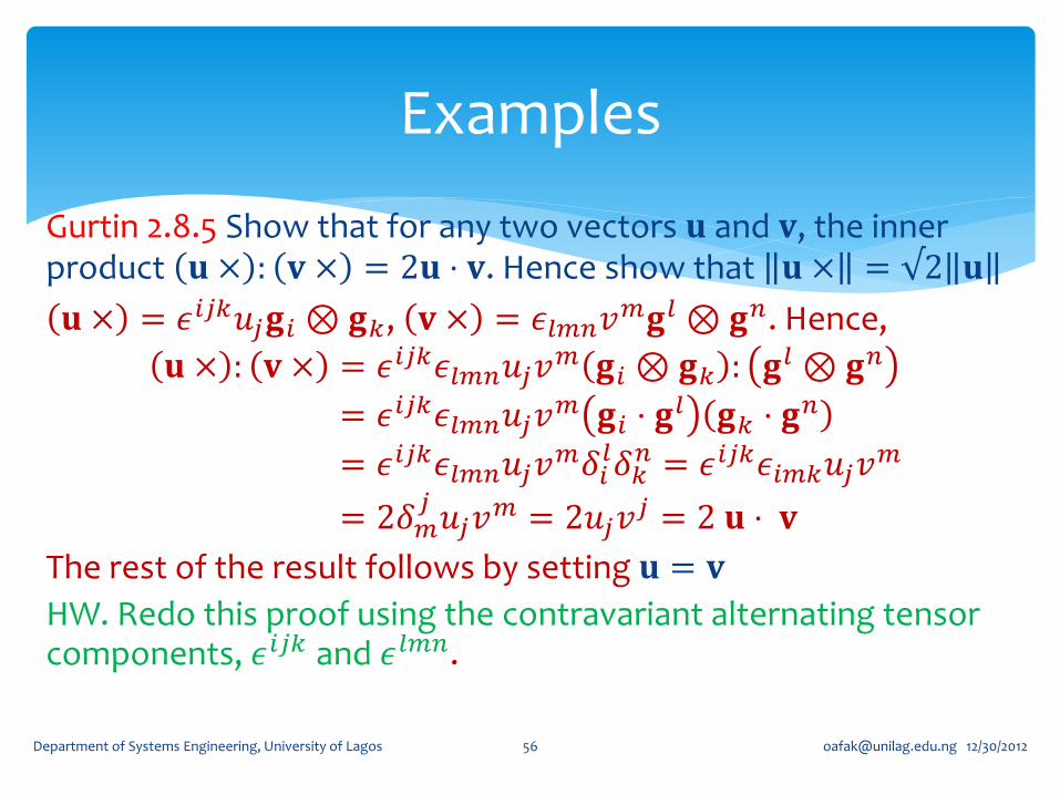
Gurtin 2.8.5 Show that for any two vectors 𝐮 and 𝐯, the inner product 𝐮 × : 𝐯 × = 2𝐮 ⋅ 𝐯. Hence show that 𝐮 × = √2 𝐮

𝐮 × = 𝜖𝑖𝑗𝑘𝑢𝑗𝐠𝑖⊗𝐠𝑘, 𝐯 × = 𝜖𝑙𝑚𝑛𝑣𝑚𝐠𝑙⊗𝐠𝑛. Hence,

𝐮 × : 𝐯 × = 𝜖𝑖𝑗𝑘𝜖𝑙𝑚𝑛𝑢𝑗𝑣𝑚 𝐠𝑖⊗𝐠𝑘 : 𝐠

𝑙⊗𝐠𝑛

= 𝜖𝑖𝑗𝑘𝜖𝑙𝑚𝑛𝑢𝑗𝑣𝑚 𝐠𝑖 ⋅ 𝐠

𝑙 𝐠𝑘 ⋅ 𝐠𝑛

= 𝜖𝑖𝑗𝑘𝜖𝑙𝑚𝑛𝑢𝑗𝑣𝑚𝛿𝑖𝑙𝛿𝑘𝑛 = 𝜖𝑖𝑗𝑘𝜖𝑖𝑚𝑘𝑢𝑗𝑣

𝑚

= 2𝛿𝑚𝑗𝑢𝑗𝑣𝑚 = 2𝑢𝑗𝑣

𝑗 = 2 𝐮 ⋅ 𝐯

The rest of the result follows by setting 𝐮 = 𝐯

HW. Redo this proof using the contravariant alternating tensor components, 𝜖𝑖𝑗𝑘 and 𝜖𝑙𝑚𝑛.


Examples

For vectors 𝐮, 𝐯 and 𝐰, show that 𝐮 × 𝐯 × 𝐰 × =𝐮⊗ 𝐯 ×𝐰 − 𝐮 ⋅ 𝐯 𝐰 ×.

The tensor 𝐮 × = −𝜖𝑙𝑚𝑛𝑢𝑛𝐠𝑙⊗𝐠𝑚

Similarly, 𝐯 × = −𝜖𝛼𝛽𝛾𝑣𝛾𝐠𝛼⊗𝐠𝛽 and 𝐰× = −𝜖𝑖𝑗𝑘𝑤𝑘𝐠𝑖⊗

𝐠𝑗. Clearly,

𝐮 × 𝐯 × 𝐰 ×

= −𝜖𝑙𝑚𝑛𝜖𝛼𝛽𝛾𝜖𝑖𝑗𝑘𝑢𝑛𝑣𝛾𝑤𝑘 𝐠𝛼⊗𝐠𝛽 𝐠

𝑙⊗𝐠𝑚 𝐠𝑖⊗𝐠𝑗= −𝜖𝛼𝛽𝛾𝜖𝑙𝑚𝑛𝜖

𝑖𝑗𝑘𝑢𝑛𝑣𝛾𝑤𝑘 𝐠𝛼⊗𝐠𝑗 𝛿𝛽𝑙 𝛿𝑖𝑚

= −𝜖𝛼𝑙𝛾𝜖𝑙𝑖𝑛𝜖𝑖𝑗𝑘𝑢𝑛𝑣𝛾𝑤𝑘 𝐠𝛼⊗𝐠𝑗

= −𝜖𝑙𝛼𝛾𝜖𝑙𝑛𝑖𝜖𝑖𝑗𝑘𝑢𝑛𝑣𝛾𝑤𝑘 𝐠𝛼⊗𝐠𝑗

= − 𝛿𝑛𝛼𝛿𝑖𝛾− 𝛿𝑖𝛼𝛿𝑛𝛾 𝜖𝑖𝑗𝑘𝑢𝑛𝑣𝛾𝑤𝑘 𝐠𝛼⊗𝐠𝑗

= −𝜖𝑖𝑗𝑘𝑢𝛼𝑣𝑖𝑤𝑘 𝐠𝛼⊗𝐠𝑗 + 𝜖𝑖𝑗𝑘𝑢𝛾𝑣𝛾𝑤𝑘 𝐠𝑖⊗𝐠𝑗

= 𝐮⊗ 𝐯 × 𝐰 − 𝐮 ⋅ 𝐯 𝐰 ×


𝑔𝑖𝑗 ≡ 𝐠𝑖 ⋅ 𝐠𝑗 and 𝑔𝑖𝑗 ≡ 𝐠𝑖 ⋅ 𝐠𝑗

These two quantities turn out to be fundamentally important to any space that which either of these two basis vectors can span. They are called the covariant and contravariant metric tensors. They are the quantities that metrize the space in the sense that any measurement of length, angles areas etc are dependent on them.

Index Raising & Lowering


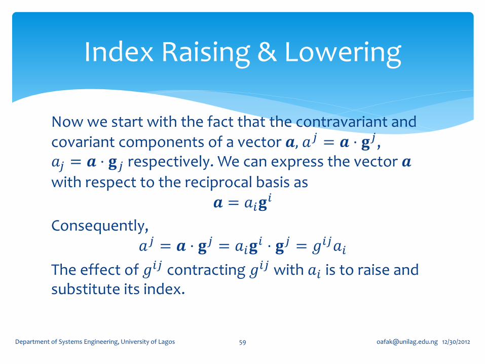
Now we start with the fact that the contravariant and covariant components of a vector 𝒂, 𝑎𝑗 = 𝒂 ⋅ 𝐠𝑗, 𝑎𝑗 = 𝒂 ⋅ 𝐠𝑗 respectively. We can express the vector 𝒂

with respect to the reciprocal basis as

𝒂 = 𝑎𝑖𝐠𝑖

Consequently, 𝑎𝑗 = 𝒂 ⋅ 𝐠𝑗 = 𝑎𝑖𝐠

𝑖 ⋅ 𝐠𝑗 = 𝑔𝑖𝑗𝑎𝑖

The effect of 𝑔𝑖𝑗 contracting 𝑔𝑖𝑗 with 𝑎𝑖 is to raise and substitute its index.



With similar arguments, it is easily demonstrated that,

𝑎𝑖 = 𝑔𝑖𝑗𝑎𝑗

So that 𝑔𝑖𝑗, in a contraction, lowers and substitutes the

index. This rule is a general one. These two components are able to raise or lower indices in tensors of higher orders as well. They are called index raising and index lowering operators.



Tensor components such as 𝑎𝑖 and 𝑎𝑗 related through the index-raising and index lowering metric tensors as we have on the previous slide, are called associated vectors. In higher order quantities, they are associated tensors.

Note that associated tensors, so called, are mere tensor components of the same tensor in different bases.

Associated Tensors


Given any tensor 𝑨, the cofactor 𝑨c of 𝑨 is the tensor

𝑻 = 𝑇𝑖.𝑗𝐠𝑖⊗𝐠𝑗 = 𝑇.𝑗

𝑖𝐠𝑖⊗𝐠𝑗

𝑇𝑚𝑙 =1

2!𝛿𝑚𝑗𝑘𝑙𝑟𝑠 𝐴𝑟

𝑗𝐴𝑠𝑘

is the cofactor of 𝑨.

Just as in a matrix, 𝑨−T = 𝑨c

det 𝑨

We now show that the tensor 𝑨c satisfies, 𝑨c 𝐮 × 𝐯 = 𝐀𝐮 × 𝐀𝐯

For any two independent vectors 𝐮 and 𝐯.

Cofactor Tensor


The above vector equation is:

𝑇𝑚𝑙 𝐠𝑙⊗𝐠

𝑚 𝜖𝑖𝑗𝑘𝑢𝑗𝑣𝑘𝐠𝑖 = 𝑇𝑚𝑙 𝜖𝑖𝑗𝑘𝑢𝑗𝑣𝑘𝛿𝑖

𝑚𝐠𝑙

= 𝑇𝑖𝑙𝜖𝑖𝑗𝑘𝑢𝑗𝑣𝑘𝐠𝑙 = 𝜖

𝑙𝑗𝑘𝐴𝑗𝑟𝐴𝑘𝑠𝑢𝑟𝑣𝑠𝐠𝑙 = 𝜖

𝑙𝑟𝑠𝐴𝑟𝑗𝐴𝑠𝑘𝑢𝑗𝑣𝑘𝐠𝑙

The coefficients of the arbitrary tensor 𝑢𝑗𝑣𝑘 are:

𝑇𝑖𝑙𝜖𝑖𝑗𝑘 = 𝜖𝑙𝑟𝑠𝐴𝑟

𝑗𝐴𝑠𝑘

Contracting on both sides with 𝜖𝑚𝑗𝑘 we have,

𝑇𝑖𝑙𝜖𝑖𝑗𝑘𝑒𝑚𝑗𝑘 = 𝜖

𝑙𝑟𝑠𝜖𝑚𝑗𝑘𝐴𝑟𝑗𝐴𝑠𝑘 so that,

2! 𝛿𝑚𝑖 𝑇𝑖𝑙 = 𝛿𝑚𝑗𝑘

𝑙𝑟𝑠 𝐴𝑟𝑗𝐴𝑠𝑘 ⇒ 𝑇𝑚

𝑙 =1

2!𝛿𝑚𝑗𝑘𝑙𝑟𝑠 𝐴𝑟

𝑗𝐴𝑠𝑘

Cofactor


The above result shows that the cofactor transforms the area vector of the parallelogram defined by 𝐮 × 𝐯 to the parallelogram defined by 𝐀𝐮 × 𝐀𝐯

Cofactor Transformation


Show that the determinant of a product is the product of the determinants

𝑪 = 𝑨𝑩 ⇒ 𝐶𝑗𝑖 = 𝐴𝑚

𝑖 𝐵𝑗𝑚

so that the determinant of 𝑪 in component form is,

𝜖𝑖𝑗𝑘𝐶𝑖1𝐶𝑗2𝐶𝑘3 = 𝜖𝑖𝑗𝑘𝐴𝑙

1𝐵𝑖𝑙𝐴𝑚2 𝐵𝑗𝑚𝐴𝑛3𝐵𝑘𝑛

= 𝐴𝑙1𝐴𝑚2 𝐴𝑛3 𝜖𝑖𝑗𝑘𝐵𝑖

𝑙𝐵𝑗𝑚𝐵𝑘𝑛

= 𝐴𝑙1𝐴𝑚2 𝐴𝑛3 𝜖𝑙𝑚𝑛 det 𝑩

= det 𝑨 × det 𝑩 .

If 𝑨 is the inverse of 𝑩, then 𝑪 becomes the identity matrix. Hence the above also proves that the determinant of an inverse is the inverse of the determinant.

Determinants


det 𝛼𝑪 = 𝜖𝑖𝑗𝑘 𝛼𝐶𝑖1 𝛼𝐶𝑗

2 𝛼𝐶𝑘3 = 𝛼3 det 𝑪

For any invertible tensor we show that det 𝑺C = det 𝑺 2

The inverse of tensor 𝑺,

𝑺−1 = det 𝑺 −1 𝑺CT

let the scalar 𝛼 = det 𝑺. We can see clearly that, 𝑺C = 𝛼𝑺−𝑇

Taking the determinant of this equation, we have,

det 𝑺C = 𝛼3 det 𝑺−𝑇 = 𝛼3 det 𝑺−1

as the transpose operation has no effect on the value of a determinant. Noting that the determinant of an inverse is the inverse of the determinant, we have,

det 𝑺C = 𝛼3 det 𝑺−1 =𝛼3

𝛼= det 𝑺 2


Show that 𝛼𝑺 C = 𝛼2𝑺C

Ans

𝛼𝑺 C = det 𝛼𝑺 𝛼𝑺 −T = 𝛼3 det 𝑺 𝛼−1𝑺−T

= 𝛼2 det 𝑺 𝑺−T = 𝛼2𝑺C

Show that 𝑺−1 C = det 𝑺 −1𝑺T

Ans. 𝑺−1 C = det 𝑺−1 𝑺−1 −𝑇 = det 𝑺 −1𝑺T

Cofactor


(HW Show that the second principal invariant of an invertible tensor is the trace of its cofactor.)

Cofactor


(d) Show that 𝑺C−1= det 𝑺 −1𝑺T

Ans. 𝑺C = det 𝑺 𝑺−𝑇

Consequently,

𝑺C−1= det 𝑺 −1 𝑺−𝑇 −1 = det 𝑺 −1𝑺T

(e) Show that 𝑺CC= det 𝑺 𝑺

Ans. 𝑺C = det 𝑺 𝑺−𝑇

So that,

𝑺CC= det 𝑺C 𝑺C

−𝑇= det 𝑺 2 𝑺C

−1 𝑇

= det 𝑺 2 det 𝑺 −1𝑺T 𝑇 = det 𝑺 2 det 𝑺 −1𝑺= det 𝑺 𝑺

as required.


3. Show that for any invertible tensor 𝑺 and any vector 𝒖,

𝑺𝒖 × = 𝑺C 𝒖 × 𝑺−𝟏

where 𝑺C and 𝑺−𝟏 are the cofactor and inverse of 𝑺 respectively.

By definition,

𝑺C = det 𝑺 𝑺−T

We are to prove that,

𝑺𝒖 × = 𝑺C 𝒖 × 𝑺−𝟏 = det 𝑺 𝑺−T 𝒖 × 𝑺−𝟏

or that,

𝑺T 𝑺𝒖 × = 𝒖 × det 𝑺 𝑺−𝟏 = 𝒖 × 𝑺C𝐓

On the RHS, the contravariant 𝑖𝑗 component of 𝒖 × is

𝒖 × 𝑖𝑗 = 𝜖𝑖𝛼𝑗𝑢𝛼

which is exactly the same as writing, 𝒖 × = 𝜖𝑖𝛼𝑙 𝑢𝛼𝐠𝑖⊗𝐠𝑙 in the invariant form.


Similarly, 𝑺C. 𝑗

𝑘 .𝐠𝑘⊗𝐠

𝑗 =1

2𝜖𝑘𝜆𝜂𝜖𝑗𝛽𝛾𝑆𝜆

𝛽𝑆𝜂𝛾𝐠𝑘⊗𝐠

𝑗 so that its transpose 𝑺CT=

1

2𝜖𝑘𝜆𝜂𝜖𝑗𝛽𝛾𝑆𝜆

𝛽𝑆𝜂𝛾𝐠𝑗⊗𝐠𝑘. We may therefore write,

𝒖 × 𝑺CT=1

2𝜖𝑖𝛼𝑙𝑢𝛼𝜖

𝑘𝜆𝜂𝜖𝑗𝛽𝛾𝑆𝜆𝛽𝑆𝜂𝛾𝐠𝑖⊗𝐠𝑙 ⋅ 𝐠

𝑗⊗𝐠𝑘

=1

2𝜖𝑖𝛼𝑙𝛿𝑙

𝑗𝑢𝛼𝜖𝑘𝜆𝜂𝜖𝑗𝛽𝛾𝑆𝜆

𝛽𝑆𝜂𝛾𝐠𝑖⊗𝐠𝑘

=1

2𝜖𝑗𝑖𝛼𝜖𝑗𝛽𝛾𝑢𝛼𝜖

𝑘𝜆𝜂𝑆𝜆𝛽𝑆𝜂𝛾𝐠𝑖⊗𝐠𝑘

=1

2𝜖𝑘𝜆𝜂 𝛿𝛽

𝑖 𝛿𝛾𝛼 − 𝛿𝛾

𝑖𝛿𝛽𝛼 𝑢𝛼𝑆𝜆

𝛽𝑆𝜂𝛾𝐠𝑖⊗𝐠𝑘

=1

2𝜖𝑘𝜆𝜂 𝑢𝛾𝑆𝜆

𝑖𝑆𝜂𝛾− 𝑢𝛽𝑆𝜆

𝛽𝑆𝜂𝑖 𝐠𝑖⊗𝐠𝑘

=1

2𝜖𝑘𝜆𝜂 𝑢𝛽𝑆𝜆

𝑖𝑆𝜂𝛽− 𝑢𝛽𝑆𝜆

𝛽𝑆𝜂𝑖 𝐠𝑖⊗𝐠𝑘 = 𝜖

𝑘𝜆𝜂𝑢𝛽𝑆𝜆𝑖𝑆𝜂𝛽𝐠𝑖⊗𝐠𝑘

= 𝜖𝑘𝛼𝛽𝑢𝑗𝑆𝛼𝑖 𝑆𝛽𝑗𝐠𝑖⊗𝐠𝑘


We now turn to the LHS;

𝑺𝒖 × = 𝜖𝑙𝛼𝑘 𝑺𝒖 𝛼𝐠𝑙⊗𝐠𝑘 = 𝜖𝑙𝛼𝑘𝑆𝛼𝑗𝑢𝑗𝐠𝑙⊗𝐠𝑘

Now, 𝑺 = 𝑆.𝛽𝑖. 𝐠𝑖⊗𝐠

𝛽 so that its transpose, 𝑺T = 𝑆𝛽𝑖𝐠𝛽⊗𝐠𝑖 = 𝑆𝑖

𝛽𝐠𝑖⊗𝐠𝛽 so that

𝑺T 𝑺𝒖 × = 𝜖𝑙𝛼𝑘𝑆𝑖𝛽𝑆𝛼𝑗𝑢𝑗𝐠𝑖⊗𝐠𝛽 ⋅ 𝐠𝑙⊗𝐠𝑘

= 𝜖𝑙𝛼𝑘𝑆𝑖𝑙𝑆𝛼𝑗𝑢𝑗𝐠𝑖⊗𝐠𝑘

= 𝜖𝑙𝛼𝑘𝑆𝑙𝑖𝑆𝛼𝑗𝑢𝑗𝐠𝑖⊗𝐠𝑘

= 𝜖𝛼𝛽𝑘𝑢𝑗𝑆𝛼𝑖 𝑆𝛽𝑗𝐠𝑖⊗𝐠𝑘 = 𝒖 × 𝑺

C T.


Show that 𝑺C𝒖 × = 𝑺 𝒖 × 𝑺T The LHS in component invariant form can be written as:

𝑺C𝒖 × = 𝜖𝑖𝑗𝑘 𝑺C𝒖𝑗𝐠𝑖⊗𝐠𝑘

where 𝑺C𝑗

𝛽=1

2𝜖𝑗𝑎𝑏𝜖

𝛽𝑐𝑑𝑆𝑐𝑎𝑆𝑑𝑏 so that

𝑺C𝒖𝑗= 𝑺C

𝑗

𝛽𝑢𝛽 =1

2𝜖𝑗𝑎𝑏𝜖

𝛽𝑐𝑑𝑢𝛽𝑆𝑐𝑎𝑆𝑑𝑏

Consequently,

𝑺C𝒖 × =1

2𝜖𝑖𝑗𝑘𝜖𝑗𝑎𝑏𝜖

𝛽𝑐𝑑𝑢𝛽𝑆𝑐𝑎𝑆𝑑𝑏𝐠𝑖⊗𝐠𝑘

=1

2𝜖𝛽𝑐𝑑 𝛿𝑎

𝑘𝛿𝑏𝑖 − 𝛿𝑏

𝑘𝛿𝑎𝑖 𝑢𝛽𝑆𝑐

𝑎𝑆𝑑𝑏𝐠𝑖⊗𝐠𝑘

=1

2𝜖𝛽𝑐𝑑𝑢𝛽 𝑆𝑐

𝑘𝑆𝑑𝑖 − 𝑆𝑐

𝑖𝑆𝑑𝑘 𝐠𝑖⊗𝐠𝑘 = 𝜖

𝛽𝑐𝑑𝑢𝛽𝑆𝑐𝑘𝑆𝑑𝑖 𝐠𝑖⊗𝐠𝑘

On the RHS, 𝒖 × 𝑺T = 𝜖𝛼𝛽𝛾𝑢𝛽𝑆𝛾𝑘𝐠𝛼⊗𝐠𝑘. We can therefore write,

𝑺 𝒖 × 𝑺T = 𝜖𝛼𝛽𝛾𝑢𝛽𝑆𝛼𝑖 𝑆𝛾𝑘𝐠𝑖⊗𝐠𝑘 =

Which on a closer look is exactly the same as the LHS so that,

𝑺C𝒖 × = 𝑺 𝒖 × 𝑺T

as required.


4. Let 𝛀 be skew with axial vector 𝝎. Given vectors 𝐮 and 𝐯, show that 𝛀𝐮 × 𝛀𝐯 = 𝝎⊗𝝎 𝐮 × 𝐯 and, hence conclude that 𝛀C = 𝝎⊗𝝎 .

𝛀𝐮 × 𝛀𝐯 = 𝝎 × 𝐮 × 𝝎 × 𝐯 = 𝝎 × 𝐮 × 𝝎 × 𝐯

= 𝝎× 𝐮 ⋅ 𝐯 𝝎 − 𝝎 × 𝐮 ⋅ 𝝎 𝐯= 𝝎 ⋅ 𝐮 × 𝐯 𝝎 = 𝝎⊗𝝎 𝐮 × 𝐯

But by definition, the cofactor must satisfy, 𝛀𝐮 × 𝛀𝐯 = 𝛀c 𝐮 × 𝐯

which compared with the previous equation yields the desired result that

𝛀C = 𝝎⊗𝝎 .


5. Show that the cofactor of a tensor can be written as

𝑺C = 𝑺2 − 𝐼1𝑺 + 𝐼2𝑰T

even if 𝑺 is not invertible. 𝐼1, 𝐼2 are the first two invariants of 𝑺.

Ans.

The above equation can be written more explicitly as,

𝑺C = 𝑺2 − tr 𝑺 𝑺 +1

2tr2 𝑺 − tr 𝑺2 𝑰

T

In the invariant component form, this is easily seen to be,

𝑺C = 𝑆𝜂 𝑖 𝑆𝑗𝜂− 𝑆𝛼𝛼𝑆𝑗𝑖 +1

2𝑆𝛼𝛼𝑆𝛽𝛽− 𝑆𝛽𝛼𝑆𝛼𝛽𝛿𝑗𝑖 𝐠𝑗⊗𝐠𝑖


But we know that the cofactor can be obtained directly from the equation,

𝑺C =1

2𝜖𝑖𝛽𝛾𝜖𝑗𝜆𝜂𝑆𝛽

𝜆𝑆𝛾𝜂𝐠𝑖⊗𝐠

𝑗 =1

2

𝛿𝑗𝑖 𝛿𝜆

𝑖 𝛿𝜂𝑖

𝛿𝑗𝛽𝛿𝜆 𝛽𝛿𝜂𝛽

𝛿𝑗𝛾𝛿𝜆 𝛾𝛿𝜂𝛾

𝑆𝛽𝜆𝑆𝛾𝜂𝐠𝑖⊗𝐠

𝑗

1

2𝛿𝑗𝑖 𝛿𝜆 𝛽𝛿𝜂𝛽

𝛿𝜆 𝛾𝛿𝜂𝛾 − 𝛿𝜆

𝑖𝛿𝑗𝛽𝛿𝜂𝛽

𝛿𝑗𝛾𝛿𝜂𝛾 + 𝛿𝜂

𝑖𝛿𝑗𝛽𝛿𝜆 𝛽

𝛿𝑗𝛾𝛿𝜆 𝛾 𝑆𝛽

𝜆𝑆𝛾𝜂𝐠𝑖⊗𝐠

𝑗

=1

2𝛿𝑗𝑖 𝛿𝜆 𝛽𝛿𝜂𝛾− 𝛿𝜂𝛽𝛿𝜆 𝛾− 𝛿𝜆 𝑖 𝛿𝑗𝛽𝛿𝜂𝛾− 𝛿𝜂𝛽𝛿𝑗𝛾 + 𝛿𝜂𝑖 𝛿𝑗𝛽𝛿𝜆 𝛾− 𝛿𝜆 𝛽𝛿𝑗𝛾𝑆𝛽𝜆𝑆𝛾𝜂𝐠𝑖⊗𝐠

𝑗

=1

2𝛿𝑗𝑖 𝑆𝛼𝛼𝑆𝛽𝛽− 𝑆𝜂𝜆𝑆𝜆 𝜂− 2𝑆𝑗

𝑖𝑆𝛼𝛼 + 2𝑆𝜂

𝑖 𝑆𝑗𝜂 𝐠𝑖⊗𝐠

𝑗


Using the above, Show that the cofactor of a vector cross 𝒖 × is 𝒖⊗𝒖

𝒖 × 2 = 𝜖𝑖𝛼𝑗𝑢𝛼𝐠𝑖⊗𝐠𝑗 𝜖𝑙𝛽𝑚𝑢𝛽𝐠𝑙⊗𝐠𝑚

= 𝜖𝑖𝛼𝑗𝜖𝑙𝛽𝑚𝑢𝛼𝑢𝛽 𝐠𝑖⊗𝐠

𝑚 𝛿𝑗𝑙 = 𝜖𝑖𝛼𝑗𝜖𝑗𝛽𝑚𝑢𝛼𝑢

𝛽 𝐠𝑖⊗𝐠𝑚

= 𝜖𝑖𝛼𝑗𝜖𝛽𝑚𝑗𝑢𝛼𝑢𝛽 𝐠𝑖⊗𝐠

𝑚

= 𝛿𝛽𝑖 𝛿𝑚𝛼 − 𝛿𝑚

𝑖 𝛿𝛽𝛼 𝑢𝛼𝑢

𝛽 𝐠𝑖⊗𝐠𝑚 = 𝑢𝑚𝑢

𝑖 − 𝛿𝑚𝑖 𝑢𝛼𝑢

𝛼 𝐠𝑖⊗𝐠𝑚

= 𝒖⊗ 𝒖 − 𝒖 ⋅ 𝒖 𝟏

tr 𝒖 × 2 = 𝒖 ⋅ 𝒖 − 3 𝒖 ⋅ 𝒖 = − 2 𝒖 ⋅ 𝒖

tr 𝒖 × = 0

But from previous result,

𝒖 × C = 𝒖 × 2 − 𝒖 × tr 𝒖 × +1

2tr2 𝒖 × − tr 𝒖 × 2 𝟏

T

= 𝒖⊗𝒖− 𝒖 ⋅ 𝒖 𝟏 − 0 +1

20 + 2 𝒖 ⋅ 𝒖 𝟏

T

= 𝒖⊗𝒖 − 𝒖 ⋅ 𝒖 𝟏 − 0 + 𝒖 ⋅ 𝒖 𝟏 T = 𝒖⊗𝒖


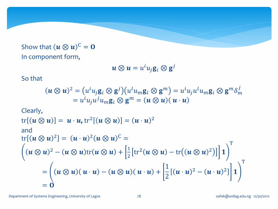
Show that 𝒖⊗𝒖 C = 𝐎

In component form,

𝒖⊗ 𝒖 = 𝑢𝑖𝑢𝑗𝐠𝑖⊗𝐠𝑗

So that

𝒖⊗ 𝒖 2 = 𝑢𝑖𝑢𝑗𝐠𝑖⊗𝐠𝑗 𝑢𝑙𝑢𝑚𝐠𝑙⊗𝐠

𝑚 = 𝑢𝑖𝑢𝑗𝑢𝑙𝑢𝑚𝐠𝑖⊗𝐠

𝑚𝛿𝑚𝑗

= 𝑢𝑖𝑢𝑗𝑢𝑗𝑢𝑚𝐠𝑖⊗𝐠

𝑚 = 𝒖⊗𝒖 𝒖 ⋅ 𝒖

Clearly,

tr 𝒖⊗ 𝒖 = 𝒖 ⋅ 𝒖, tr2 𝒖⊗𝒖 = 𝒖 ⋅ 𝒖 2

and tr 𝒖⊗ 𝒖 2 = 𝒖 ⋅ 𝒖 2 𝒖⊗𝒖 C =

𝒖⊗𝒖 2 − 𝒖⊗ 𝒖 tr 𝒖⊗ 𝒖 +1

2tr2 𝒖⊗𝒖 − tr 𝒖⊗ 𝒖 2 𝟏

T

= 𝒖⊗𝒖 𝒖 ⋅ 𝒖 − 𝒖⊗𝒖 𝒖 ⋅ 𝒖 +1

2𝒖 ⋅ 𝒖 2 − 𝒖 ⋅ 𝒖 2 𝟏

T

= 𝐎


Given a Euclidean Vector Space E, a tensor 𝑸 is said to be orthogonal if, ∀𝒂, 𝒃 ∈ E,

𝑸𝒂 ⋅ 𝑸𝒃 = 𝒂 ⋅ 𝒃 Specifically, we can allow 𝒂 = 𝒃, so that

𝑸𝒂 ⋅ 𝑸𝒂 = 𝒂 ⋅ 𝒂

Or 𝑸𝒂 = 𝒂

In which case the mapping leaves the magnitude unaltered.

Orthogonal Tensors


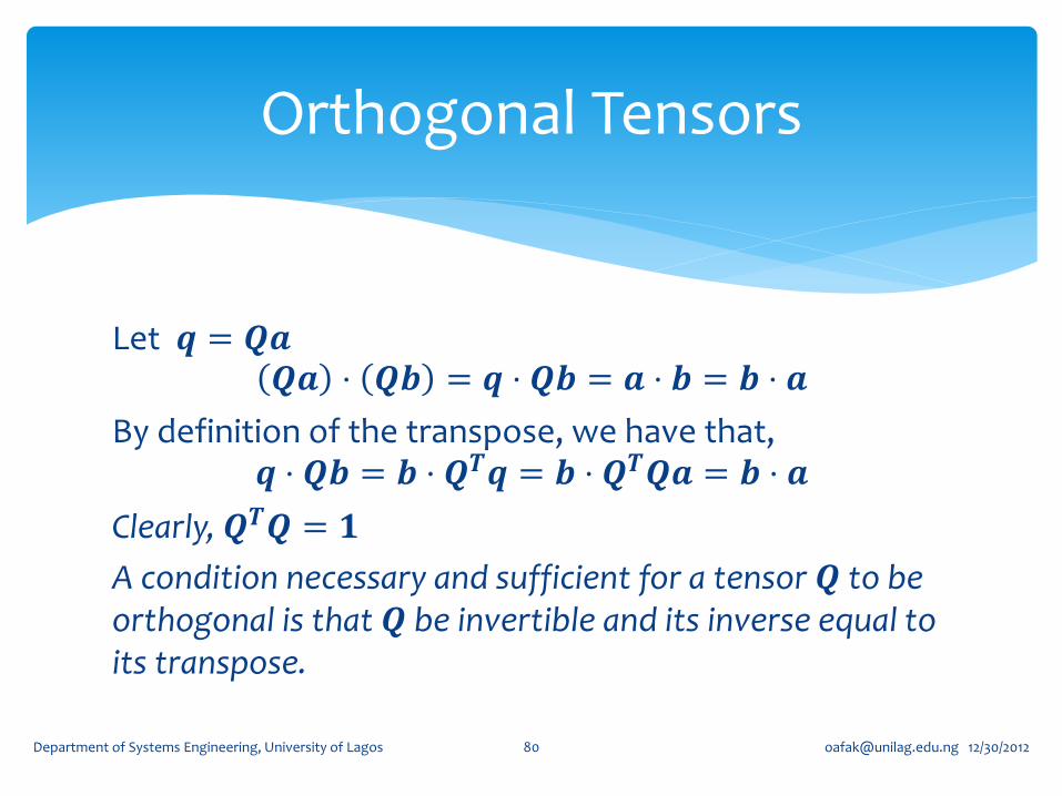
Let 𝒒 = 𝑸𝒂 𝑸𝒂 ⋅ 𝑸𝒃 = 𝒒 ⋅ 𝑸𝒃 = 𝒂 ⋅ 𝒃 = 𝒃 ⋅ 𝒂

By definition of the transpose, we have that, 𝒒 ⋅ 𝑸𝒃 = 𝒃 ⋅ 𝑸𝑻𝒒 = 𝒃 ⋅ 𝑸𝑻𝑸𝒂 = 𝒃 ⋅ 𝒂

Clearly, 𝑸𝑻𝑸 = 𝟏

A condition necessary and sufficient for a tensor 𝑸 to be orthogonal is that 𝑸 be invertible and its inverse equal to its transpose.

Orthogonal Tensors


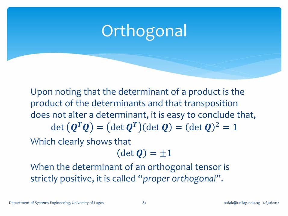
Upon noting that the determinant of a product is the product of the determinants and that transposition does not alter a determinant, it is easy to conclude that,

det 𝑸𝑻𝑸 = det 𝑸𝑻 det 𝑸 = det 𝑸 2 = 1

Which clearly shows that det 𝑸 = ±1

When the determinant of an orthogonal tensor is strictly positive, it is called “proper orthogonal”.

Orthogonal


A rotation is a proper orthogonal tensor while a reflection is not.

Rotation & Reflection


Let 𝑸 be a rotation. For any pair of vectors 𝐮, 𝐯 show that 𝑸 𝐮 × 𝐯 = (𝑸𝐮) × (𝑸𝐯)

This question is the same as showing that the cofactor of 𝑸 is 𝑸 itself. That is that a rotation is self cofactor. We can write that

𝑻 𝐮 × 𝐯 = (𝑸𝐮) × (𝑸𝐯)

where 𝐓 = cof 𝑸 = det 𝑸 𝑸−T

Now that 𝑸 is a rotation, det 𝑸 = 1, and 𝑸−T = (𝑸−1)𝑇 = (𝑸T)𝑇 = 𝑸

This implies that 𝑻 = 𝑸 and consequently, 𝑸 𝐮 × 𝐯 = (𝑸𝐮) × (𝑸𝐯)

Rotation


For a proper orthogonal tensor Q, show that the eigenvalue equation always yields an eigenvalue of +1. This means that there is always a solution for the equation,

𝑸𝒖 = 𝒖

For any invertible tensor, 𝑺C = det 𝑺 𝑺−T

For a proper orthogonal tensor 𝑸, det 𝑸 = 1. It therefore follows that,

𝑸C = det𝑸 𝑸−T = 𝑸−T = 𝑸

It is easily shown that tr𝑸C = 𝐼2(𝑸) (HW Show this Romano 26)

Characteristic equation for 𝑸 is, det 𝑸 − 𝜆𝟏 = 𝜆3 − 𝜆2𝑄1 + 𝜆𝑄2 − 𝑄3 = 0

Or, 𝜆3 − 𝜆2𝑄1 + 𝜆𝑄1 − 1 = 0

Which is obviously satisfied by 𝜆 = 1.


If for an arbitrary unit vector 𝐞, the tensor, 𝑸 𝜃 = cos 𝜃 𝑰 + (1 − cos 𝜽 )𝐞 ⊗𝐞 + sin 𝜃 (𝐞 ×) where (𝐞 ×) is the skew tensor whose 𝑖𝑗 component is 𝝐𝒋𝒊𝒌𝒆𝒌,

show that 𝑸 𝜃 (𝑰 − 𝐞⊗ 𝐞) = cos 𝜃 (𝑰 − 𝐞⊗ 𝐞) + sin 𝜃 (𝐞 ×).

𝑸 𝜃 𝐞⊗ 𝐞 = cos 𝜃 𝐞 ⊗ 𝐞 + (1 − cos 𝜽 )𝐞⊗ 𝐞 + sin 𝜃 [𝐞 × 𝐞⊗ 𝐞 ]

The last term vanishes immediately on account of the fact that 𝐞⊗ 𝐞 is a symmetric tensor. We therefore have,

𝑸 𝜃 𝐞⊗ 𝐞 = cos 𝜃 𝐞 ⊗ 𝐞 + (1 − cos 𝜽 )𝐞 ⊗ 𝐞 = 𝐞⊗ 𝐞

which again mean that 𝑸 𝜃 so that

𝑸 𝜃 𝑰 − 𝐞⊗ 𝐞 = cos 𝜃 𝑰 + 1 − cos 𝜽 𝐞 ⊗ 𝐞 + sin 𝜃 𝐞 × − 𝐞⊗ 𝐞

= 𝑐os 𝜃 𝑰 − 𝐞⊗ 𝐞 + sin 𝜃 𝐞 × as required.


If for an arbitrary unit vector 𝐞, the tensor, 𝑸 𝜃 = cos 𝜃 𝑰 + (1 − cos 𝜽 )𝐞 ⊗𝐞 + sin 𝜃 (𝐞 ×) where (𝐞 ×) is the skew tensor whose 𝑖𝑗 component is 𝜖𝑗𝑖𝑘𝑒𝑘.

Show for an arbitrary vector 𝐮 that 𝐯 = 𝑸 𝜃 𝐮 has the same magnitude as 𝐮.

Given an arbitrary vector 𝐮, compute the vector 𝐯 = 𝑸 𝜃 𝐮. Clearly, 𝐯 = cos 𝜃 𝐮 + 1 − cos 𝜽 𝐮 ⋅ 𝐞 𝐞 + sin 𝜃 𝐞 × 𝐮

The square of the magnitude of 𝐯 is

𝐯 ⋅ 𝐯 = 𝐯 𝟐 = cos2𝜃 𝐮 ⋅ 𝐮 + 1 − cos 𝜽 𝟐 𝐮 ⋅ 𝐮 𝟐 + sin2 𝜃 𝐞 × 𝐮 2

+ 2 cos 𝜽 1 − cos 𝜽 𝐮 ⋅ 𝐞 𝟐

= cos2𝜃 𝐮 ⋅ 𝐮 + 1 − cos 𝜽 𝐮 ⋅ 𝐞 𝟐 1 − cos 𝜽 + 𝟐 cos 𝜽+ sin2 𝜃 𝐞 × 𝐮 2

= cos2𝜃 𝐮 ⋅ 𝐮 + 1 − cos 𝜽 𝐮 ⋅ 𝐞 𝟐 1 + cos 𝜽 + sin2 𝜃 𝐞 × 𝐮 2

= cos2𝜃 𝐮 ⋅ 𝐮 + 1 − cos2 𝜽 𝐮 ⋅ 𝐞 𝟐 + sin2 𝜃 𝐞 × 𝐮 2

= cos2𝜃 𝐮 ⋅ 𝐮 + sin2 𝜃 𝐮 ⋅ 𝐞 𝟐 + 𝐞 × 𝐮 2

= cos2𝜃 𝐮 ⋅ 𝐮 + sin2 𝜃 𝐮 ⋅ 𝐮 = 𝐮 ⋅ 𝐮.

The operation of the tensor 𝑸 𝜃 on 𝐮 is independent of 𝜃 and does not change the magnitude. Furthermore, it is also easy to show that the projection 𝐮 ⋅ 𝐞 of an arbitrary vector on 𝐞 as well as that of its image 𝐯 ⋅ 𝐞 are the same. The axis of rotation is therefore in the direction of 𝐞.


If for an arbitrary unit vector 𝐞, the tensor, 𝑸 𝜃 = cos 𝜃 𝑰 + (1 − cos 𝜽 )𝐞⊗ 𝐞 +sin 𝜃 (𝐞 ×) where (𝐞 ×) is the skew tensor whose 𝑖𝑗 component is 𝝐𝒋𝒊𝒌𝒆𝒌. Show for an arbitrary 0 ≤ 𝛼, 𝛽 ≤ 2𝜋, that 𝑸 𝛼 + 𝛽 = 𝑸 𝛼 𝑸 𝛽 .

It is convenient to write 𝑸 𝛼 and 𝑸 𝛽 in terms of their components: The ij component of

𝑸 𝛼 𝑖𝑗 = (cos𝛼)𝛿𝑖𝑗 + 1 − cos𝛼 𝑒𝑖𝑒𝑗 − (sin 𝛼) 𝜖𝑖𝑗𝑘𝑒𝑘

Consequently, we can write,

𝑸 𝛼 𝑸 𝛽 𝑖𝑗 = 𝑸 𝛼 𝒊𝒌 𝑸 𝛽 𝑘𝑗 =

= (cos𝛼)𝛿𝑖𝑘 + 1 − cos𝛼 𝑒𝑖𝑒𝑘 − (sin 𝛼) 𝜖𝑖𝑘𝑙𝑒𝑙 (cos𝛽)𝛿𝑘𝑗+ 1 − cos𝛽 𝑒𝑘𝑒𝑗 − (sin𝛽) 𝜖𝑘𝑗𝑚𝑒𝑚 = (cos𝛼 cos𝛽) 𝛿𝑖𝑘𝛿𝑘𝑗 + cos𝛼(1 − cos𝛽)𝛿𝑖𝑘𝑒𝑘𝑒𝑗 − cos𝛼 sin 𝛽 𝜖𝑘𝑗𝑚𝑒𝑚𝛿𝑖𝑘

+ cos𝛽(1 − cos𝛼)𝛿𝑘𝑗𝑒𝑖𝑒𝑘 + 1 − cos𝛼 1 − cos𝛽 𝑒𝑖𝑒𝑘𝑒𝑘𝑒𝑗− 1 − cos𝛼 𝑒𝑖𝑒𝑘 (sin 𝛽) 𝜖𝑘𝑗𝑚𝑒𝑚 − (sin𝛼 cos𝛽) 𝜖𝑖𝑘𝑙𝑒𝑙𝛿𝑘𝑗− (sin𝛼) 1 − cos𝛽 𝑒𝑘𝑒𝑗 𝜖𝑖𝑘𝑙𝑒𝑙 + (sin𝛼 sin 𝛽) 𝜖𝑖𝑘𝑙𝜖𝑘𝑗𝑚𝑒𝑙𝑒𝑚 = (cos𝛼 cos𝛽) 𝛿𝑖𝑗 + cos𝛼(1 − cos𝛽)𝑒𝑖𝑒𝑗 − cos𝛼 sin 𝛽 𝜖𝑖𝑗𝑚𝑒𝑚

+ cos𝛽(1 − cos𝛼)𝑒𝑖𝑒𝑗 + 1 − cos𝛼 1 − cos𝛽 𝑒𝑖𝑒𝑗 − (sin𝛼 cos𝛽) 𝜖𝑖𝑗𝑙𝑒𝑙+ (sin𝛼 sin𝛽) 𝛿𝑙𝑗𝛿𝑖𝑚 − 𝛿𝑙𝑚𝛿𝑗𝑖 𝑒𝑙𝑒𝑚 = (cos𝛼 cos𝛽 − sin 𝛼 sin 𝛽) 𝛿𝑖𝑗 + 1 − ( cos αcos𝛽 − sin 𝛼 sin 𝛽) 𝑒𝑖𝑒𝑗

− cos𝛼 sin 𝛽 − sin 𝛼 cos𝛽 𝜖𝑖𝑗𝑚𝑒𝑚 = 𝑸 𝛼 + 𝛽 𝑖𝑗


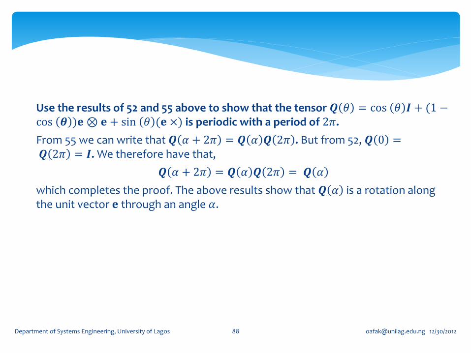
Use the results of 52 and 55 above to show that the tensor 𝑸 𝜃 = cos 𝜃 𝑰 + (1 −cos 𝜽 )𝐞 ⊗ 𝐞 + sin 𝜃 (𝐞 ×) is periodic with a period of 2𝜋.

From 55 we can write that 𝑸 𝛼 + 2𝜋 = 𝑸 𝛼 𝑸 2𝜋 . But from 52, 𝑸 0 = 𝑸 2𝜋 = 𝑰. We therefore have that,

𝑸 𝛼 + 2𝜋 = 𝑸 𝛼 𝑸 2𝜋 = 𝑸 𝛼

which completes the proof. The above results show that 𝑸 𝛼 is a rotation along the unit vector 𝐞 through an angle 𝛼.


Define Lin+as the set of all tensors with a positive determinant. Show that Lin+is invariant under G where is the proper orthogonal group of all rotations, in the sense that for any tensor 𝐀 ∈ Lin+ 𝐐 ∈ G ⇒ 𝐐𝐀𝐐T ∈ Lin+ .(G285)

Since we are given that 𝐀 ∈ Lin+, the determinant of 𝐀 is positive. Consider

det 𝐐𝐀𝐐T . We observe the fact that the determinant of a product of tensors is

the product of their determinants (proved above). We see clearly that,

det 𝐐𝐀𝐐T = det 𝐐 × det 𝐀 × det 𝐐T . Since 𝐐 is a rotation, det 𝐐 =

det 𝐐T = 1. Consequently we see that,

det 𝐐𝐀𝐐T = det 𝐐 × det 𝐀 × det 𝐐T

= det 𝐐𝐀𝐐T

= 1 × det 𝐀 × 1 = det 𝐀

Hence the determinant of 𝐐𝐀𝐐T is also positive and therefore 𝐐𝐀𝐐T ∈ Lin+ .


Define Sym as the set of all symmetric tensors. Show that Sym is invariant under G where is the proper orthogonal group of all rotations, in the sense that for any tensor A ∈ Sym every 𝐐 ∈ 𝐺 ⇒ 𝐐𝐀𝐐T ∈ Sym. (G285)

Since we are given that A ∈ Sym, we inspect the tensor 𝐐𝐀𝐐T. Its transpose is,

𝐐𝐀𝐐TT= 𝐐T

T𝐀𝐐T = 𝐐𝐀𝐐T. So that 𝐐𝐀𝐐T is symmetric and therefore

𝐐𝐀𝐐T ∈ Sym. so that the transformation is invariant.


Central to the usefulness of tensors in Continuum Mechanics is the Eigenvalue Problem and its consequences.

• These issues lead to the mathematical representation of such physical properties as Principal stresses, Principal strains, Principal stretches, Principal planes, Natural frequencies, Normal modes, Characteristic values, resonance, equivalent stresses, theories of yielding, failure analyses, Von Mises stresses, etc.

• As we can see, these seeming unrelated issues are all centered around the eigenvalue problem of tensors. Symmetry groups, and many other constructs that simplify analyses cannot be understood outside a thorough understanding of the eigenvalue problem.

• At this stage of our study of Tensor Algebra, we shall go through a simplified study of the eigenvalue problem. This study will reward any diligent effort. The converse is also true. A superficial understanding of the Eigenvalue problem will cost you dearly.


Recall that a tensor 𝑻 is a linear transformation for 𝒖 ∈ V

𝑻: V → V

states that ∃ 𝒘 ∈ V such that, 𝑻𝒖 ≡ 𝑻 𝒖 = 𝒘

Generally, 𝒖 and its image, 𝒘 are independent vectors for an arbitrary tensor 𝑻. The eigenvalue problem considers the special case when there is a linear dependence between 𝒖 and 𝒘.

The Eigenvalue Problem


Here the image 𝒘 = 𝜆𝒖 where 𝜆 ∈ R 𝑻𝒖 = 𝜆𝒖

The vector 𝒖, if it can be found, that satisfies the above equation, is called an eigenvector while the scalar 𝜆 is its corresponding eigenvalue.

The eigenvalue problem examines the existence of the eigenvalue and the corresponding eigenvector as well as their consequences.

Eigenvalue Problem


In order to obtain such solutions, it is useful to write out this equation in its component form:

𝑇𝑗𝑖𝑢𝑗𝐠𝑖 = 𝜆𝑢

𝑖𝐠𝑖

so that,

𝑇𝑗𝑖 − 𝜆𝛿𝑗

𝑖 𝑢𝑗𝐠𝑖 = 𝐨

the zero vector. Each component must vanish identically so that we can write


𝑖 𝑢𝑗 = 0


From the fundamental law of algebra, the above equations can only be possible for arbitrary values of 𝑢𝑗 if the determinant,


𝑖

Vanishes identically. Which, when written out in full, yields,

𝑇11 − 𝜆 𝑇2

1 𝑇31

𝑇12 𝑇2

2 − 𝜆 𝑇32

𝑇13 𝑇2

3 𝑇33 − 𝜆

= 0


Expanding, we have,

−𝑇31𝑇22𝑇13 + 𝑇2

1𝑇32𝑇13 + 𝑇3

1𝑇12𝑇23 − 𝑇1

1𝑇32𝑇23 − 𝑇2

1𝑇12𝑇33

+ 𝑇11𝑇22𝑇33 + 𝑇2

1𝑇12𝜆 − 𝑇1

1𝑇22𝜆 + 𝑇3

1𝑇13𝜆 + 𝑇3

2𝑇23𝜆

− 𝑇11𝑇33𝜆 − 𝑇2

2𝑇33𝜆 + 𝑇1

1𝜆2 + 𝑇22𝜆2 + 𝑇3

3𝜆2 − 𝜆3

= 0

= −𝑇31𝑇22𝑇13 + 𝑇2

1𝑇32𝑇13 + 𝑇3

1𝑇12𝑇23 − 𝑇1

1𝑇32𝑇23 − 𝑇2

1𝑇12𝑇33

+ 𝑇11𝑇22𝑇33

+ (𝑇21𝑇12 − 𝑇1

1𝑇22 + 𝑇3

1𝑇13 + 𝑇3

2𝑇23 − 𝑇1

1𝑇33

− 𝑇22𝑇33)𝜆 + 𝑇1

1 + 𝑇22 + 𝑇3

3 𝜆2 − 𝜆3 = 0

or 𝜆3 − 𝐼1𝜆

2 + 𝐼2𝜆 − 𝐼3 = 0


This is the characteristic equation for the tensor 𝑻. From here we are able, in the best cases, to find the three eigenvalues. Each of these can be used in to obtain the corresponding eigenvector.

The above coefficients are the same invariants we have seen earlier!

Principal Invariants Again


A tensor 𝑻 is Positive Definite if for all 𝒖 ∈ V , 𝒖 ⋅ 𝑻𝒖 > 0

It is easy to show that the eigenvalues of a symmetric, positive definite tensor are all greater than zero. (HW: Show this, and its converse that if the eigenvalues are greater than zero, the tensor is symmetric and positive definite. Hint, use the spectral decomposition.)

Positive Definite Tensors


We now state without proof (See Dill for proof) the important Caley-Hamilton theorem: Every tensor satisfies its own characteristic equation. That is, the characteristic equation not only applies to the eigenvalues but must be satisfied by the tensor 𝐓 itself. This means,

𝐓3 − 𝐼1𝐓2 + 𝐼2𝐓 − 𝐼3𝟏 = 𝑶

is also valid.

This fact is used in continuum mechanics to obtain the spectral decomposition of important material and spatial tensors.

Cayley- Hamilton Theorem


It is easy to show that when the tensor is symmetric, its three eigenvalues are all real. When they are distinct, corresponding eigenvectors are orthogonal. It is therefore possible to create a basis for the tensor with an orthonormal system based on the normalized eigenvectors. This leads to what is called a spectral decomposition of a symmetric tensor in terms of a coordinate system formed by its eigenvectors:

𝐓 = 𝜆𝑖

3

𝑖=1

𝐧𝑖⨂𝐧𝑖

Where 𝐧𝑖 is the normalized eigenvector corresponding to the eigenvalue 𝜆𝑖.

Spectral Decomposition


The above spectral decomposition is a special case where the eigenbasis forms an Orthonormal Basis. Clearly, all symmetric tensors are diagonalizable.

Multiplicity of roots, when it occurs robs this representation of its uniqueness because two or more coefficients of the eigenbasis are now the same.

The uniqueness is recoverable by the ingenious device of eigenprojection.

Multiplicity of Roots


Case 1: All Roots equal.

The three orthonormal eigenvectors in an ONB obviously constitutes an Identity tensor 𝟏. The unique spectral representation therefore becomes

𝐓 = 𝜆𝑖

3

𝑖=1

𝐧𝑖⨂𝐧𝑖 = 𝜆 𝐧𝑖⨂𝐧𝑖

3

𝑖=1

since 𝜆1 = 𝜆2 = 𝜆3 = 𝜆 in this case.

Eigenprojectors


Case 2: Two Roots equal: 𝜆1unique while 𝜆2 = 𝜆3

In this case, 𝐓 = 𝜆1𝐧1⨂𝐧1 + 𝜆2 𝟏 − 𝐧1⨂𝐧1

since 𝜆2 = 𝜆3 in this case.

The eigenspace of the tensor is made up of the projectors: 𝑷1 = 𝐧1⨂𝐧1

and 𝑷2 = 𝟏 − 𝐧2⨂𝐧2

Eigenprojectors


The eigen projectors in all cases are based on the normalized eigenvectors of the tensor. They constitute the eigenspace even in the case of repeated roots. They can be easily shown to be:

1. Idempotent: 𝑷𝑖 𝑷𝑖 = 𝑷𝑖 (no sums)

2. Orthogonal: 𝑷𝑖 𝑷𝑗 = 𝑶 (the anihilator)

3. Complete: 𝑷𝑖 = 𝟏𝑛𝑖=1 (the identity)

Eigenprojectors


For symmetric tensors (with real eigenvalues and consequently, a defined spectral form in all cases), the tensor equivalent of real functions can easily be defined:

Trancendental as well as other functions of tensors are defined by the following maps:

𝑭:Sym → Sym

Maps a symmetric tensor into a symmetric tensor. The latter is the spectral form such that,

𝑭 𝑻 ≡ 𝑓(𝜆𝑖)𝐧𝑖⨂𝐧𝑖

3

𝑖=1

Tensor Functions


Where 𝑓(𝜆𝑖) is the relevant real function of the ith eigenvalue of the tensor 𝑻.

Whenever the tensor is symmetric, for any map, 𝑓:R →R, ∃ 𝑭:Sym → Sym

As defined above. The tensor function is defined uniquely through its spectral representation.

Tensor functions


Show that the principal invariants of a tensor 𝑺 satisfy

𝑰𝒌 𝑸𝑺𝑸T = 𝐼𝑘 𝑺 , 𝑘 = 1,2, or 3 Rotations and orthogonal

transformations do not change the Invariants

𝐼1 𝑸𝑺𝑸T = tr 𝑸𝑺𝑸T = tr 𝑸T𝑸𝑺 = tr 𝑺 = 𝐼1(𝑺)

𝐼2 𝑸𝑺𝑸T =1

2tr2 𝑸𝑺𝑸T − tr 𝑸𝑺𝑸T𝑸𝑺𝑸T

=1

2I12 𝑺 − tr 𝑸𝑺𝟐𝑸T

=1

2I12 𝑺 − tr 𝑸T𝑸𝑺𝟐

=1

2I12(𝑺) − tr 𝑺𝟐 = 𝐼2(𝑺)

𝐼3 𝑸𝑺𝑸T = det 𝑸𝑺𝑸T

= det 𝑸T𝑸𝑺 = det 𝑺 = 𝐼3 𝑺

Hence 𝐼𝑘 𝑸𝑺𝑸T = 𝐼𝑘 𝑺 , 𝑘 = 1,2, or 3


Show that, for any tensor 𝑺, tr 𝑺2 = 𝐼12(𝑺) − 2𝐼2 𝑺 and

tr 𝑺3 = 𝐼13 𝑺 − 3𝐼1𝐼2 𝑺 + 3𝐼3 𝑺

𝐼2 𝑺 =1

2tr2 𝑺 − tr 𝑺2

=1

2𝐼12(𝑺) − tr 𝑺2

So that, tr 𝑺2 = 𝐼1

2(𝑺) − 2𝐼2 𝑺

By the Cayley-Hamilton theorem, 𝑺3 − 𝐼1𝑺

2 + 𝐼2𝑺 − 𝐼3𝟏 = 𝟎

Taking a trace of the above equation, we can write that, tr 𝑺3 − 𝐼1𝑺

2 + 𝐼2𝑺 − 𝐼3𝟏 = tr(𝑺3) − 𝐼1tr 𝑺

2 + 𝐼2tr 𝑺 − 3𝐼3 = 0

so that, tr 𝑺3 = 𝐼1 𝑺 tr 𝑺

2 − 𝐼2 𝑺 tr 𝑺 + 3𝐼3 𝑺

= 𝐼1 𝑺 𝐼12 𝑺 − 2𝐼2 𝑺 − 𝐼1 𝑺 𝐼2 𝑺 + 3𝐼3 𝑺

= 𝐼13 𝑺 − 3𝐼1𝐼2 𝑺 + 3𝐼3 𝑺

As required.


Suppose that 𝑼 and 𝑪 are symmetric, positive-definite tensors with 𝑼2 = 𝑪, write the invariants of C in terms of U

𝐼1 𝑪 = tr 𝑼2 = 𝐼1

2(𝑼) − 2𝐼2 𝑼

By the Cayley-Hamilton theorem, 𝑼3 − 𝐼1𝑼

2 + 𝐼2𝑼 − 𝐼3𝑰 = 𝟎

which contracted with 𝑼 gives, 𝑼4 − 𝐼1𝑼

3 + 𝐼2𝑼2 − 𝐼3𝑼 = 𝟎

so that, 𝑼4 = 𝐼1𝑼

3 − 𝐼2𝑼2 + 𝐼3𝑼

and tr 𝑼4 = 𝐼1tr 𝑼

3 − 𝐼2tr 𝑼2 + 𝐼3tr 𝑼

= 𝐼1 𝑼 𝐼13 𝑼 − 3𝐼1 𝑼 𝐼2 𝑼 + 3𝐼3 𝑼

− 𝐼2 𝑼 𝐼12 𝑼 − 2𝐼2 𝑼 + 𝐼1 𝑼 𝐼3 𝑼

= 𝐼14 𝑼 − 4𝐼1

2 𝑼 𝐼2 𝑼 + 4𝐼1 𝑼 𝐼3 𝑼 + 2𝐼22 𝑼


But,

𝐼2 𝑪 =1

2𝐼12 𝑪 − tr 𝑪2 =

1

2𝐼12 𝑼2 − tr 𝑼4

=1

2tr2 𝑼2 − tr 𝑼4

=1

2𝐼12 𝑼 − 2𝐼2 𝑼

2− tr 𝑼4

=1

2 𝐼14 𝑼 − 4𝐼1

2 𝑼 𝐼2 𝑼 + 4𝐼22 𝑼

− 𝐼14 𝑼 − 4𝐼1

2 𝑼 𝐼2 𝑼 + 4𝐼1 𝑼 𝐼3 𝑼 + 2𝐼22 𝑼

The boxed items cancel out so that, 𝐼2 𝑪 = 𝐼2

2 𝑼 − 2𝐼1 𝑼 𝐼3 𝑼

as required. 𝐼3 𝑪 = det 𝑪 = det 𝑼

2 = det 𝑼 2 = 𝐼32 𝑼


tensor algebra - oafak.comoafak.com/wp-content/uploads/2013/01/2-tensor-algebra-jan-2013.pdftensor...

Documents