algebra and coalgebra on categorical tensor network states
TRANSCRIPT

Algebra and Coalgebra on Categorical Tensor Network States
Jacob D Biamonte1, ∗
1Oxford University Computing Laboratory
We present a set of new tools which extend the problem solving techniques and
range of applicability of network theory as currently applied to quantum many-body
physics. We use this new framework to give a solution to the quantum decompo-
sition problem. Specifically, given a quantum state S, we are now able to directly
construct a tensor network that describes the state S. This solution became pos-
sible by synthesizing and tailoring several powerful modern techniques from higher
mathematics: category theory, algebra and coalgebra and applicable results from
classical network theory and graphical calculus. We present several examples (such
as categorical MERA networks etc.) which illustrate how the established methods
surrounding tensor network states arise as a special instance of this more general
framework, which we call Categorical Tensor Network States.

2
I. MOTIVATION SUMMARY: A NEW QUANTUM NETWORK THEORY
We report the development of a new tool set and corresponding framework which is sig-
nificantly different and outside the range of methods used to address problems in network
descriptions of many-body physics and related disciplines. In the categorical network model
of quantum states we present, each of the internal components that form our network building
blocks are completely defined in terms of their mathematical properties, and these proper-
ties are given in terms of equations which have a purely graphical interpretation: category
theory [1] replaces ad hoc graphical methods in network descriptions of many-body physics
and e.g. enables rigorous proofs to now be done graphically. We went out of our way to write
this article for a general reader with a background in tensor network states and/or quantum
circuit theory: no background in category theory or higher algebra is assumed.
To explain the key motivation behind developing this new machinery, let us recall the
success of established numerical simulation methods, such as density matrix renormalization
group (DMRG) and quantum Monte Carlo (QMC) which have become key to studying
strongly correlated systems in regimes and at scales where quantum mechanical effects are
crucial [2, 3]. However, substantial limitations have remained in the size, dimensionality,
and classes of Hamiltonians these methods can be used to simulate.
Tensor network states arose recently from the field of Quantum Information Science as
the backbone of applicable and general methods to simulate quantum systems using classi-
cal computers. As a matter of necessity, and one of opportunity, by utilizing concepts from
quantum information science several novel and powerful computer algorithms (all based on
tensor network states) have recently been proposed which have overcome many existing
numerical limitations. Specifically: the Multi-scale Entanglement Renormalization Ansatz
(MERA) [4] and Projected Entangled Pairs (PEPS) [5] — see also [6–8]. In addition, tensor
network based numerical algorithms have recently been successfully adapted to the simula-
tion of stochastic classical systems [9]. These and other related methods have been used to
perform highly accurate calculations on a broad class of strongly correlated systems. This
has attracted significant interest from several research communities concerned with computer
simulations of physical systems.
Computer Science techniques such as semantics and logic emerged out of increasingly

3
general methods to depict intuitive and descriptive models of systems and processes. Such
conceptual methods rely on the unifying language of category theory [10, 11]: for both its
expressive power and as a unification tool to uniformly reason over wide classes of a priori
seemingly different scenarios. Many otherwise obscure aspects of mathematical models can
be made vivid at the level of Categories, and the associated differences can be pinpointed
on-the-nose in terms of clear, definable structure. This continues to set the stage for the
formal analysis of a range of generally applicable scientific concepts.
The expressiveness and range of applicability of tensor network based algorithmic tech-
niques is fostered by an intuitive graphical language describing the tensor networks which
represent physical states and processes. This graphical language can now take a broader
direction by being connected to the long existing rigorous language of Category Theory.
This will immediately open the door to apply many established techniques: category theory
provides the exact arena of mathematics concerned with such diagrammatic reasoning. The
diagrammatic language of tensor network states in current use is a special case of this long
existing rich framework. Again, as stated, we present the category theory underpinning our
approach with a wide audience in mind — this work is largely self contained and assumes
little if any knowledge of higher algebra or category theory. We will explore several category
theoretic results that arose from this study in future publications.
Categorical models of tensor network states allow us to both “zoom out” and expose
high-level structure, but also to “zoom in” and expose hosts of “hidden” algebraic structures
that are not currently being considered in the tensor network simulation community. En-
hancing the graphical language component of these numerical methods should lead to the
discovery new theoretical models and numerical algorithms which challenge and shape our
understanding of many-body physics.
Category theory is often used as a unifying language for mathematics [1] and in more
recent times to formulate physical theories [10, 11]. To accomplish our goals, we will build
on ideas across several fields. This includes the work by Lafont [12] which was aimed at
providing an algebraic theory for classical Boolean circuits. We represent this algebraic
theory on tensors and use these to express quantum states. Using more Category Theory
tightens this approach and removes some redundancy in his graphical lemmas [12]. Lafont’s
work is related to the more recent work on proof theory by Guiraud [13]. One of the

4
strong points of categorical modeling is that it comes equipped with many flavors of intuitive
graphical calculi. We consider a so-called Penrose-Joyal-Street calculus (and actually the
Kelly-Laplaza-Selinger coherence result [1, 14, 15]) and as a matter of convenience, we make
use of †-compactness already present in categorical quantum theory [16]. The graphical
calculus formally extends to a rigorous tool. See for instance, Selinger’s survey of graphical
languages for monoidal categories (these are the categories which describe Hilbert spaces
and quantum theory [15]).
II. RESULTS OVERVIEW: IIA, II B AND IIC
We will now quickly introduce the key concepts of this paper before going into full detail
in the remaining sections. The main idea (representing quantum states in terms of networks)
is reviewed next in IIA with the corresponding algebraic definitions of these network compo-
nents reviewed in II B and the concept of a state defining an algebra in II C. We summarize
this new theory in IID and outline the structure of the remainder of the manuscript in III.
These first three review sections (IIA, II B and IIC) where made accessible for the range of
readers working in the area of quantum information science with a background in quantum
circuits, and/or the existing tensor network theory.
A. A New Representation of Quantum States
We give algebraic operations a representation on quantum states. This allows us to
do the converse, that is, give tensor network states a representation in terms of algebraic
operations! The starting point of classical network theory was seminal work resulting in
Shannon and Davio decompositions of functions into networks. These powerful methods
formed the backbone and enabled the last century of methods surrounding classical network
theory. The present paper presents a solution to the related quantum problem: that is, the
decomposition of a quantum state into a categorical tensor network.
To get an idea of what we’re about to do, let’s consider a key network building block:
the so-called “quantum AND-state” which we define in Section IVD and was given in [17].
This is a representation of the familiar Boolean operation in the bit pattern of a tri-qubit
5
quantum state as
ψANDdef=
∑x1,x2,x3=0/1
|x1〉 ⊗ |x2〉 ⊗ |x1 ∧ x2〉 = |000〉+ |010〉+ |100〉+ |111〉 (1)
and hence, the truth table of a function is encoded in the bit pattern of the superposition.
This gives rise to a linear representation of Boolean gates (represented on quantum states)
as opposed to the typical direct sum representation common in Boolean algebra.
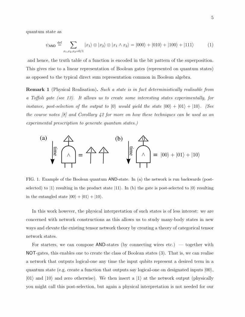
Remark 1 (Physical Realisation). Such a state is in fact deterministically realisable from
a Toffoli gate (see 13). It allows us to create some interesting states experimentally, for
instance, post-selection of the output to |0〉 would yield the state |00〉 + |01〉 + |10〉. (See
the course notes [8] and Corollary 42 for more on how these techniques can be used as an
experimental prescription to generate quantum states.)
= =
(a) (b)
time
time
FIG. 1. Example of the Boolean quantum AND-state. In (a) the network is run backwards (post-
selected) to |1〉 resulting in the product state |11〉. In (b) the gate is post-selected to |0〉 resulting
in the entangled state |00〉+ |01〉+ |10〉.
In this work however, the physical interpretation of such states is of less interest: we are
concerned with network constructions as this allows us to study many-body states in new
ways and elevate the existing tensor network theory by creating a theory of categorical tensor
network states.
For starters, we can compose AND-states (by connecting wires etc.) — together with
NOT-gates, this enables one to create the class of Boolean states (3). That is, we can realise
a network that outputs logical-one any time the input qubits represent a desired term in a
quantum state (e.g. create a function that outputs say logical-one on designated inputs |00〉,
|01〉 and |10〉 and zero otherwise). We then insert a |1〉 at the network output (physically
you might call this post-selection, but again a physical interpretation is not needed for our

6
purposes). This recovers the desired Boolean state
1
2n/2
∑x1,x2,...,xn=0/1
〈1|f(x1, x2, ..., xn)〉|x1, x2, ..., xn〉 (2)
where in terms of a network, we read the network backwards from output to input (a related
idea arose in my work on adiabatic circuits [18]). This full class of Boolean states is defined
as:
Definition 2 (Boolean Many-Body Quantum States). We define the class of Boolean states
as those states which can be expressed up to a scalar in the form∑x1,x2,...,xn=0/1
|x1, x2, ..., xn〉|f(x1, x2, ..., xn)〉 (3)
where f is a switching function and the abusive notation in the sum is over all variables
taking 0 and 1.
Our full method subsumes the important class of Boolean states as a subclass. In fact,
we’re able to translate any quantum state directly into a categorical tensor network. This
appears to open a door: a new and different research direction in quantum network theory
by providing a new handle on quantum states. This is captured by the following result (see
Theorem 35).
Result 3 (Translating Quantum States into Categorical Tensor Networks). Given quantum
state |S〉, Theorem 35 asserts a constructive (efficient in poly(k, n) classical computing re-
sources) method to represent |S〉 in a categorical tensor network with poly(k, n) rank-3 and
rank-2 tensors.
An attractive aspect of our approach is that we’re able to place the network components
into clearly defined building blocks. Indeed, these building blocks are defined in terms of a
rich graphical language — we utilize the theory of Monoidal Categories [1] and related ideas
in computer science for this.
B. Network components fully defined by diagrammatic laws
The theory of Categories provides a framework to elevate diagrammatic reasoning to a
rigorous tool — e.g. proofs can be done graphically! We will in addition, use this framework

7
to fully define the algebraic operations appearing in this work, and this definition will be done
graphically. This picture calculus can be used whenever working in the the dagger-category
(that is †-category) of von Neumann quantum mechanics (for details see [15, 16]).
To get an idea of how this will work, consider Figure 2, which forms a presentation of
the linear fragment of the Boolean calculus: that is, the calculus of Boolean algebra we
represent on quantum states, restricted to the building blocks that can be used to generate
linear Boolean functions.
(a) (b) (c)
==
(d)
=
=
= =
=
=
=
=
=
(e)
(f)
(g)
FIG. 2. Read top to bottom. A presentation of the linear fragment of the Boolean calculus. The
plus (⊕) dots are XOR and the black (•) dots represent COPY. The details of (a)-(g) will be given
in Sections IV and V. For instance, (d) represents the bialgebra law and (g) the Hopf-law (in this
case true as x⊕ x = 0).
To recover the full Boolean-calculus, we must consider a non-linear Boolean gate: we use
AND-gates and Figure 2 together with Figure 3 to form a full presentation of the calculus [12].
As stated, in this work, we will give the Boolean-calculus a representation (on quantum
states) and make use of the categorical generalisation of map-state duality found first in [16,
19], and which we studied in the setting on quantum circuits and called cup/cap induced
duality in [20].
Remark 4 (Full Set of Defining Equations). We note that the presentations in Figure 2
together with Figure 3 are not just a set of relations and identities on circuit components,
but instead represent a complete set of defining equations [21].
We need to add a bit more to the presentation of the Boolean calculus to represent
quantum states. Proceeding systematically by adding just a bit more structure we’re able
to do a whole lot more. One way forward is to add what are called compact structures in
8
(a) (b) (c) (d)
=
=
=
=
(f) (h)
==
=
=
= =
(g)(e)
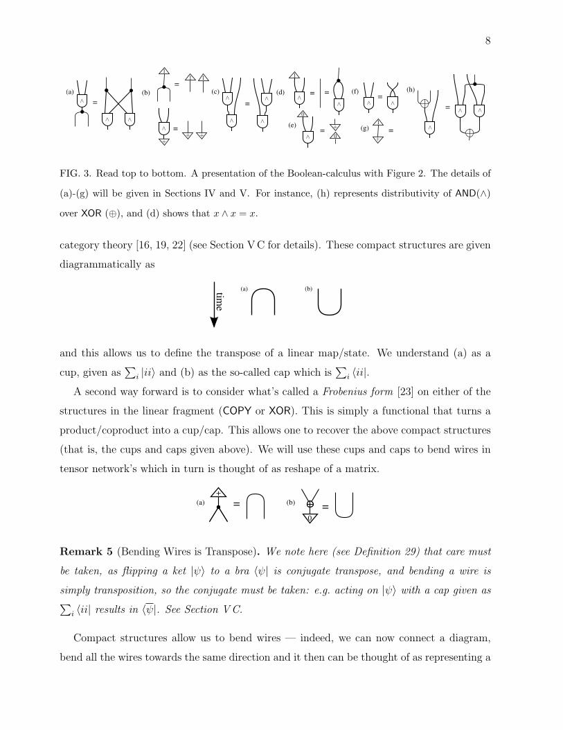
FIG. 3. Read top to bottom. A presentation of the Boolean-calculus with Figure 2. The details of
(a)-(g) will be given in Sections IV and V. For instance, (h) represents distributivity of AND(∧)
over XOR (⊕), and (d) shows that x ∧ x = x.
category theory [16, 19, 22] (see Section VC for details). These compact structures are given
diagrammatically as
(a) (b)time
and this allows us to define the transpose of a linear map/state. We understand (a) as a
cup, given as∑
i |ii〉 and (b) as the so-called cap which is∑
i 〈ii|.
A second way forward is to consider what’s called a Frobenius form [23] on either of the
structures in the linear fragment (COPY or XOR). This is simply a functional that turns a
product/coproduct into a cup/cap. This allows one to recover the above compact structures
(that is, the cups and caps given above). We will use these cups and caps to bend wires in
tensor network’s which in turn is thought of as reshape of a matrix.
=
+
=0
(a) (b)
Remark 5 (Bending Wires is Transpose). We note here (see Definition 29) that care must
be taken, as flipping a ket |ψ〉 to a bra 〈ψ| is conjugate transpose, and bending a wire is
simply transposition, so the conjugate must be taken: e.g. acting on |ψ〉 with a cap given as∑i 〈ii| results in 〈ψ|. See Section VC.
Compact structures allow us to bend wires — indeed, we can now connect a diagram,
bend all the wires towards the same direction and it then can be thought of as representing a

9
state, bend them the other way and it then can be thought of as representing a measurement
outcome, that is, an effect. One can also connect inputs to outputs, creating larger and larger
networks. What’s more is that these compact structures have a vivid physical meaning in
terms of an algebra on quantum states. A clunky (less user friendly) variant of this algebra
on quantum states is already present in categorical quantum theory [8, 22] — it was cleaned
up a bit and basically made more user friendly for physicists in [8]. We will clarify this
algebraic structure on quantum states and explain its physical meaning next. We however
again mention that most of what we consider here is simply an abstract network theory, and
the physical interpretations of these operations, and their interactions in terms of quantum
mechanics, is not really necessary for applications in numerical algorithms involving tensor
network simulation.
C. A new type of algebra on quantum states
We are concerned with a network theory of quantum states. This on the one hand can
be used as a tool to solve problems about states and operators in quantum theory, but does
have a physical interpretation on the other. This is largely based on what you might call
an operational interpretation of quantum states and processes. An algebra is a pairing on a
vector space, taking two vectors and producing a third (you might call it a monoid if there
is a unit). Let’s now see how every tripartite quantum state forms an algebra.
Consider a tripartite quantum state (subsystems labeled 1,2 and 3), and ask the simple
question, how would the state of the third system change after we measure systems one and
two? Enter Algebras: as stated, an algebra on a vector space, or on a Hilbert space is formed
by a product taking two elements from the vector space to produce a third element in the
vector space. Algebra on states can then be studied by considering duality of the state, that
is considering the adjunction between the maps of type
1 → H⊗H⊗H and H⊗H → H (4)
This duality is made evident by using the †-compact structure of the category (e.g. the cups
and caps). It is given vivid physical meaning by considering the effect measuring (that is
two events) two components of a state has on the third component.

10
Remark 6 (Overbar notation on Spaces). Given a Hilbert space H, we can consider the
Hilbert space H which can be simply thought of as the Hilbert space H will all basis vectors
complex conjugates (overbar). That is, H is a vector space whose elements are in one-to-one
correspondence with the elements of H:
H = {v | v ∈ H}, (5)
with the following rules for addition and scalar multiplication:
v + w = v + w and α v = α v . (6)
Remark 7 (Definition of Algebra). We consider an algebra as a vector space A endowed
with a product, taking a pair of elements (e.g. from A⊗A) and producing an element in A.
So the product is a map A⊗A → A, which may not be associative or have a unit (that is,
a multiplicative identity — see 18 for an example of an algebra on a quantum state without
a unit).
Observation 8 (Every tripartite Quantum State Forms an Algebra). Let ψ ∈ H⊗H⊗H be a
quantum state and let Mi, Mj be complete sets of measurement operators. Then (ψ,Mi,Mj)
forms an algebra.
= := =
time
The quantum state is drawn as a triangle, with the identity operator on each subsystem
acting as time goes to the right on the page. Projective measurements with respect to Mi
and Mj are made. We define these complete measurement operators as
M1 =N∑i=1
i · |ψi〉〈ψi| (7)
M2 =N∑j=1
j · |φj〉〈φj| (8)

11
such that we recover the identity operator on the N -level subsystem viz
N∑j=1
|φj〉〈φj| =N∑i=1
|ψi〉〈ψi| = 1N (9)
The measurements result in eigenvalues i, j leaving the state of the unmeasured system in
|ω〉 =∑
x1,x2,x3
〈ψi|x1〉〈φj|x2〉|x3〉 (10)
where 〈Q| def= |Q〉> that is, the transpose is factored into: (i) taking the dagger (diagram-
matically this mirrors states across the page) and (ii) taking the complex conjugate. Hence,
〈Q|†= |Q〉> = 〈Q| = 〈Q|† (11)
and if we pick a real valued basis for x1, x2, x3 we recover
|ω〉 =∑
x1,x2,x3
〈x1|ψi〉〈x2|φj〉|x3〉 (12)
As stated, this physical interpretation is not our main interest. It’s a nice feature, but
even in its absence, we’re able to write down and represent a quantum state purely in terms
of a connected network, where each component is fully defined in terms of algebraic laws.
D. Putting it all together: connecting the dots
This new formalism allows us to express a range of new a priori hidden tensor network
structure. Indeed, as we mentioned categorical tensor network states allow us to both “zoom
out” and expose high-level structure, but also to “zoom in” and expose hosts of algebraic
structures that are not currently being considered in the tensor network simulation commu-
nity. As will be shown, by formally defining these network building blocks, we’re able to see
a lot more of what’s going on inside these networks. Importantly, we’re able to do things
that are not possible using the current approach to tensor network states: translate a given
quantum state directly into a representative network. This provides a quantum network
analog of classical network decomposition methods.
We hope that presenting a solution to the quantum decomposition problem and that by
enhancing the graphical language component of these numerical methods, that our work will
lead to new theoretical models and numerical algorithms which will challenge and shape our
understanding of many-body physics.

12
III. REMAINING MANUSCRIPT STRUCTURE
We have organized this manuscript in the following way: We continue next in IV by
defining our network building blocks including rank-3 tensors such as defining the quantum
AND-state in Equation 18. We then consider how these components interact in Section V.
This is done in terms of algebraic laws, such as Bialgebra (VB) and Hopf-algebras (VB1).
With these definitions in place, we’re able to continue onto Section VI: we applying this
framework to create a new type of tensor network theory. We zoom in and expose internal
structure of an MPS and particularly consider categorical tensor networks for many-body W-
states in VI. An example categorical MERA network along with reduced two- and four-point
correlation functions (graphically in our language) are given in Section VID. In conclusion,
we mention some future directions in VII and importantly, how this work opens the door
to apply tensor network simulation methods to NP-complete problems. We have included
Appendix A on the Boolean XOR-algebra we represent on quantum states.
a. Assumed Background. We assume readers are familiar with the basics of tensor
network states (see the reviews in [5, 24]). We have gone out of our way to make the category
theory necessary in this work as user friendly as possible. For general background see [1]
and for more related work see [8, 20]. In a further attempt to make this document readable
across the range of people working on these topics, we assume only minimal knowledge of
Boolean algebra, discrete set functions and circuit theory (see a quick review of XOR-algebra
in Appendix A and more generally see [25] and [26] for background on pseudo Boolean
functions). We assume readers have experience with quantum circuits and basic quantum
computing concepts (e.g. at the level of [8, 27, 28]).
Remark 9 (Normalisation factors omitted). As one would expect in quantum theory, where
rays describe the state space, without loss of generality we will often omit global scale factors
mainly for ease of presentation. We note that for Hilbert space H there is a truly natural
isomorphism
C⊗H ∼= H ∼= H⊗ C (13)
where the ⊗ of a scalar M and a vector S becomes regular multiplication as M ⊗S =M ·S.
Remark 10 (Diagrammatic conventions: top to bottom and left to right). Diagrams will
typically be drawn with ‘time’ going down the page. However, in certain instances we will

13
draw them from left to right across the page to aid in presentation. We note that in general
open legs can be attached to other open legs (contracted) and that nodes, maps, etc. all have
evident meaning, which should be clear from context.
IV. CONSTITUENT NETWORK COMPONENTS
Any vector space V has a dual V∗: this is the space of linear functions f from V to the
ground field C, that is f : V → C. This defines the dual uniquely. We must however fix
a basis to identify the vector space V with its dual. Given a basis, any basis vector ei in
V gives a basis vector f j in V∗ defined by f j(ei) = δji (Kronecker’s delta). This defines an
isomorphism V → V∗ sending ei to fi and allowing us to identify V with V∗. In what follows,
we will fix a particular arbitrarily chosen basis (called the computational basis in quantum
information science). We will proceed to give only the necessary building blocks that are
needed in our construction.
A. COPY: the “diagonal”
The copy operation arises in digital circuits and more generally, in the context of category
theory and Algebra, where it is called a diagonal in cartesian categories. (although not
directly relevant for the present work, see [29] for details on using COPY to define a basis).
The operation is defined as
4 def=
∑i
|ii〉〈i| (14)
where the sum is over ∀i which could be, e.g. iterating a complete Boolean basis: for qubits,
that is i = 0, 1. As |0〉 and |1〉 are eigenstates of σz, we might give 4 the alternative
name of Z-copy (this was done in [22, 29] when considering COPY as a quantum observable)
— which in the case of qubits is succinctly presented by considering the map that copies
σz-eigenstates:
4 : C2 → C2 ⊗ C2 ::
|0〉 7→ |00〉
|1〉 7→ |11〉
This map can be written as 4 : |00〉〈0|+ |11〉〈1| and under cup/cap induced duality (on the
right bra) this state becomes a GHZ -state as ψGHZ = |000〉+ |111〉. The standard properties

14
of COPY are given diagrammatically in Figure 4 and a list of its relevant mathematical
properties are found in Figure 5.
(a) (b)
=
(c)
==
(d)
=
time
time
tim
e
=
FIG. 4. The COPY-dot. (a) Full-symmetry. (b) Copy points, e.g. |x〉 7→ |xx〉 for x = 0, 1. (c) The
unit — in this case the unit corresponds to deletion, or a map to the terminal object |+〉 def= |0〉+ |1〉
(the bi-direction of time is explained in by considering co-diagonals in IVE). (d) Co-interaction
with the unit creates a Bell state. This is the compact structure of the †-category of quantum
theory.
Remark 11 (The COPY-gate from CNOT). The CNOT-gate is defined as |0〉〈0|1 ⊗ 12 +
|1〉〈1|1⊗σx2 . We will set the input that the target acts on to |0〉 we then calculate CNOT(11⊗
|0〉2) = |0〉〈0|1 ⊗ |0〉2 + |1〉〈1|1 ⊗ |1〉2. We have hence defined the desired map (COPY) from
the Hilbert space with label 1 (subscript) to the joint Hilbert space labeled 1 and 2.
Gate Type Co-copy point(s) Unit Co-unit Interaction
COPY |0〉,|1〉 (b) |+〉 (c) Bell state: |00〉+ |11〉 (d)
Symmetry Associative Commutative Frobenius Algebra
Full (a) Yes Yes Yes (Spider Law)
FIG. 5. Summary of the COPY-gate.
B. XOR: the “addition”
The XOR-gate logic gate that implements exclusive disjunction or addition (mod 2) —
written with symbol ⊕. By what could be called “dot-duality”, the XOR-gate is simply a
Hadamard transform of the COPY-gate, applied to all of the dots legs. This can be captured
diagrammatically in the slightly different form

15
=
which clarifies several examples. To define the gate on the computational basis, we consider
f(x1, x2) = x1 ⊕ x2 then f = 0 corresponds to (x1, x2) = (0, 0), (1, 1) and f = 1 corresponds
to (x1, x2) = (1, 0), (0, 1), where the truth table for XOR follows
x1 x2 f(x1, x2) = x1 ⊕ x2
0 0 0
0 1 1
1 0 1
1 1 0
Under cap/cap induced duality, the state defined by XOR is given as
ψ⊕def=
∑x1,x2
|x1〉|x2〉|f(x1, x2)〉 = |000〉+ |110〉+ |011〉+ |101〉 (15)
which is in the GHZ -class — by LOCC equivalence viz. ψ⊕ = H⊗H⊗H(|000〉+ |111〉). The
operation of XOR is summarized in the table appearing in Figure 6. Since the XOR-gate is
related to the COPY-gate by a change of basis its diagrammatic laws have the same structure
as those already appearing in Figure 4. The gate acting backwards (co-XOR) is defined on
a basis by
⊕ : C2 → C2 ⊗ C2 ::
|0〉 7→ |00〉+ |11〉
|1〉 7→ |10〉+ |01〉or equivalently
|+〉 7→ |++〉
|−〉 7→ | − −〉
Gate Type Co-copy point(s) Unit Co-unit Interaction
XOR |+〉,|−〉 (b) |0〉 (c) Bell state: |00〉+ |11〉 (d)
Symmetry Associative Commutative Frobenius Algebra
Full (a) Yes Yes Yes (Spider Law)
FIG. 6. Summary of the XOR-gate.

16
C. The constant 1: negation
Linear Boolean functions, are functions which have uncomplimented variables that appear
individually (e.g. variable couplings are not allowed such as x1x2 etc. see A). Linear functions
take the general form
f(x1, x2, ..., xn) = c1x1 ⊕ c2x2 ⊕ ...⊕ cnxn (16)
where the vector (c1, c2, ..., cn) determines the function. The affine boolean functions are
linear functions that allow variables to appear in both complimented and uncomplimented
form. Affine functions take the general form
f(x1, x2, ..., xn) = c0 ⊕ c1x1 ⊕ c2x2 ⊕ ...⊕ cnxn (17)
where c0 = 1 gives functions outside the linear class. Together, XOR and COPY are not
universal for classical circuits. However, When used in conjunction, XOR- and COPY-gates
compose to create the class of linear circuits. The affine circuits are generated by considering
constant |1〉. This point (|1〉) is indeed copied by the black dot. However, an axomitisation
can proceed through only considering the XOR- and COPY-gates together with |+〉, the unit
for COPY and |0〉 the unit for XOR. It is by appending the constant |1〉 into the system that
the affine class of circuits can be realised.
Remark 12 (Affine functions correspond to a basis). Each affine function is labeled by a
corresponding bit pattern. This forms a function basis for the space of Boolean polynomials
and can also be thought of as labeling the computational basis (see A).
D. Quantum AND-states: enter Boolean non-linearity
AND (that is, ∧) implements logical conjunction. By what could be called “dot-duality”,
the AND-gate relates to the OR-gate via De Morgan’s law. This can be captured diagram-
matically as
=

17
To define the gate on the computational basis, we consider f(x1, x2) = x1 ∧ x2 which we
write as x1x2. Here f = 0 corresponds to (x1, x2) = (0, 0), (0, 1), (1, 0) and f = 1 corresponds
to (x1, x2) = (1, 1), where the truth table for AND follows
x1 x2 f(x1, x2) = x1 ∧ x20 0 0
0 1 0
1 0 0
1 1 1
Under cap/cap induced duality, the state defined by AND is given as
ψ∧def=
∑x1,x2
|x1〉|x2〉|f(x1, x2)〉 = |000〉+ |010〉+ |010〉+ |111〉 (18)
The operation of AND is summarized in the table appearing in Figure 6. The gate acting
backwards is defined on a basis as and its key diagrammatic properties are presented in
Figure 7
∧ : C2 → C2⊗C2 ::
|0〉 7→ |00〉+ |01〉+ |10〉
|1〉 7→ |11〉or
|+〉 7→ |++〉
|−〉 7→ |00〉+ |01〉+ |10〉 − |11〉
(a) (b)
=
(c)
==
(d)
time
tim
e=
tim
e
FIG. 7. The AND-gate. (a) Input-symmetry. (b) Existence of a zero or fixed-point. (c) The unit
|1〉. (d) Co-interaction with the unit creates a product-state. Note that the gate forms a valid
quantum operation when run backwards as in (d).
Example 13 (AND-states from Toffoli-gates). The AND-state is readily constructed from
the ‘ as illustrated in Figure 8.
Gate Type Co-copy point(s) Unit Co-unit Interaction
AND |1〉 (b) |1〉 (c) Product state: |11〉 (d)
Symmetry Associative Commutative Bialgebra Law
Inputs (a) Yes Yes Yes (with GHZ )

18
FIG. 8. Illustrates the use of compact structures for black and plus dots to prepare the state
ψAND = |000〉+ |010〉+ |100〉+ |111〉. Using only single qubit NOT-gates, one can use this method
to construct any of the states representing the non-linear Boolean functions in Figure 9. We note
that the box around the Toffoli gate (left) is meant to illustrate that those two connected dots do
not satisfy the spider-law 22.
Remark 14 (Universal States). We should note that quantum universal diagrams are possi-
ble by considering simple Hadamard states (e.g. ψH = |00〉+|01〉+|10〉−|11〉) and AND-states.
This follows from the simple proof that Hadamard and Toffoli are quantum universal [30].
E. co-COPY: the co-diagonal
It should be evident from the preceding discussions that our gates are what a physicist
would call tensors (with the evident graphical interpretation apparently first pointed out
in [31]) and that open legs on tensor correspond to say spin degrees of freedom (and are
hence either states or dual to states by bending wires). In this manner, we say that gates
can be used both forwards in backwards in time.
We already mentioned in the results summary that we utilize the †-compact structure
from categorical quantum theory to take the adjoint of a linear map. This let’s us take the
transpose (e.g. bend wires). What happens if we flip a copy operation upside down, that
is, instead of having a single leg split into two legs, have two legs merge into one. The first
thing one might ask is if this is physical?
Appending a physical interpretation to these operations in terms of a quantum process
is possible, by considering, e.g. post-selection, but not necessary for our purposes. Indeed,
this is not our goal here as we’re concerned with representing states in terms of categorical

19
tensor networks — we expose an elegant, user friendly language to accomplish just that. So
the co-COPY is simply thought of as a being a dual (transpose) to the familiar COPY.
This is common in algebra: to consider the dual notation to algebra, that is co-algebra.
In general, while a product is a joining or paring (e.g. taking two vectors and producing a
third) a co-product is a co-pairing taking a single vector in say A and producing a vector in
A⊗A.
Remark 15 (Coalgebras). Coalgebras are structures that are dual (in the sense of revers-
ing arrows) to unital associative algebras such as COPY and AND the axioms of which we
formulated in terms of picture calculi (IVA and IVD). Every coalgebra, by (vector space)
duality, gives rise to an algebra, and in finite dimensions, this duality goes in both directions.
Co-COPY can be thought of as applying a delta function in the transition from input to
output. That is, given a copy point x
4 (|x〉) = |x〉 ⊗ |x〉 (19)
we have that
5 (|i〉, |j〉) = δij|i〉 (20)
that is, the diagram get’s mapped to zero (or empty) if the inputs don’t agree. This is
succiently written in terms of a Delta-function dependent on inputs i, j.
Example 16 (Simple co-pairing). Measurement effects on tri-state quantum systems can
be thought of as a coproducts. This is given as a map from one system (measuring the
first) into two systems (the effect this has on the other two). GHZ -states are prototypical
examples of co-pairings: an example left to the reader to explore.
F. The remaining Boolean states: NAND-states etc.
We have represented a complete logical system on quantum states — this enables us to
represent any Boolean function quantum mechanically and hence any Boolean state. We
chose as our generators, constant |1〉, COPY, XOR, AND. Other generators could have also
been chosen. Our choice however, was made as a matter of convenience, as the definitions
work well, and elegantly fit together (e.g. representing the XOR-algebra). If we would have

20
considered other generators, we could have ended up considering the following cases: weak-
units (17) and fixed point pairs (19).
Definition 17 (Weak Units). An algebra (or product) on a tri-party state ψ has a unit
(equivalently the state is unital) if there exists an effect φ which the product acts on to
produce an invertible map B, where B = 1 (see Example 18). If no such φ exists to make
B = 1, and B has an inverse, we call φ a weak unit, and say the state ψ is weak unital
and if B 6= 1 and B2 = 1 we call the algebra on ψ unital-involutive. This scenario is given
diagrammatically as:
= =
Example 18 (NAND and NOR). NAND and NOR have weak units, respectively given by
|1〉 and |0〉. These weak units are unital-involutive.
ψNAND = |001〉+ |011〉+ |011〉+ |110〉 (21)
ψNOR = |001〉+ |010〉+ |100〉+ |110〉 (22)
For ψNAND to have a unit, there must exist a |φ〉 such that
〈φ|0〉|01〉+ 〈φ|0〉|11〉+ 〈φ|0〉|11〉+ 〈φ|1〉|10〉 (23)
is equal to the Bell-state |00〉+ |11〉 and hence dual to |1〉〈1|+ |0〉〈0|. No choice of |φ〉 makes
this possible.
Definition 19 (Fixed Point Pair). An algebra on a tri-party state ψ has a Fixed Point if
there exists an effect φ making the output constant. If the constant is output and φ are both
|0〉, we say φ has a zero. A fixed point pair consists of two algebras with fixed points, such
that the fixed point of one algebra is the unit of the other, and vise versa (see Example 20).
Diagrammatically this is expressed in the following:
==
Example 20 (AND, OR form a Fixed Point Pair). AND and OR form a fixed point pair.
That is, the unit for AND (|1〉 see a) is the zero for OR (c) and vise versa: the unit of OR
(|0〉 see a) is the zero for AND (b).

21
(a) (b) (c)
== = =
G. Summarizing: Network Composition of Quantum Logic States
We have considered set’s of universal classical structures in the categorical tensor network
model. In classical computer science, a universal set of gates, is able to express any n-bit
Boolean function
f : Bn → B :: (x1, ..., xn) 7→ f(x1, ..., xn) (24)
Universal sets include {COPY, NAND}, {COPY, AND, NOT}, {COPY, AND, XOR,1},
{OR, XNOR,1} and others. One can also consider the states ψ formed by the bit pat-
terns of these functions f(a, b) as
ψf =∑
a,b∈{0,1}
|a〉|b〉|f(a, b)〉 (25)
This allows a wide class of states to be constructed effectively. In the following Table (9) we
illustrate the states representing the classical function of two-inputs.
Remark 21 (Induced compact structure). The Boolean states in Table (9) represent true
tri-state entanglement. For each state, there exists an effect (a measurement outcome) on
one of the states that leaves the other two parties in an entangled state. Mathematically, this
entangled state defines what’s called a non-degenerate pairing.
V. INTERACTION OF THE NETWORK COMPONENTS
1. Merging Dots: Spider Law
Copy dots are readily generalized to an arbitrary number of input and output legs. As
one would rightly suspect, a copy dot with n inputs and m outputs corresponds to an n+m-

22
non-linear linear (Frobenius Algebras)
ψAND = |000〉+ |010〉+ |100〉+ |111〉
ψOR = |001〉+ |011〉+ |101〉+ |111〉 ψXOR = |000〉+ |011〉+ |101〉+ |110〉
ψNAND = |001〉+ |011〉+ |101〉+ |110〉 ψXNOR = |001〉+ |010〉+ |100〉+ |111〉
ψNOR = |001〉+ |010〉+ |100〉+ |110〉
FIG. 9. The bit pattern of these quantum states represents a Boolean function (given by the
subscript) such that the right most bit is the Boolean functions output, and the two left bits are
the functions inputs, and the non-linear Boolean functions are on the left side of the table and the
linear functions on the right. Consider the state ψAND, and Boolean variables x1 and x2, then the
superposition ψAND encodes the function |x1, x2, x1 ∧ x2〉 in each term in the superposition, and
ψAND =∑
x1,x2∈{0,1} |x1, x2, x1 ∧ x2〉. As outlined in the text, cup/cap induced-duality allows us
(for instance) to express this state as the operator |0〉〈00|+ |0〉〈01|+ |0〉〈01|+ |1〉〈11| :: |x1, x2〉 7→
|x1 ∧ x2〉 which projects qubit states to the AND of their bit value.
partite GHZ state. Neighboring dots of the same color can be merged into a single dot: just
like in digital circuits.
Theorem 22 (Spider Law [22, 23]). Given a connected graph with m inputs and n outputs
comprised solely of Frobenius dots of equal dimension, this map can be equivalently expressed
as a single m-to-n dot, as shown in Figure 10.
Example 23 (Two-site reduced density operator of n-party GHZ -states). GHZ -states on
n-parties have a well known matrix product expression given as
GHZn = Tr
|0〉 0
0 |1〉
n
= |00...0〉+ |11...1〉 (26)
where the internal matrix product is given by ⊗. These MPS networks are known to be
efficiently contactable. We note that the networks in Figure 10 are not a priori in a con-
tractible form due to the number of of open legs. What makes them contractible (in their
present from) is the spider law. The reduced density matrix of an n-party GHZ -state then
becomes (a) in Figure 11 and the expectation value of an observable is shown in (b). where
we include the normalisation constant.

23
FIG. 10. Spider law: connected black-dots (•) as well as connected plus-dots (⊕) can be merged.
=
(a) (b)
=
FIG. 11. Reduced density operator. Left (a) reduced density operator ρ′GHZ found from applying
the spider law to a n-qubit GHZ -state. Right (b) the expectation value of observable O1 ⊗ O2
found from connecting the observable and connecting the open legs (e.g. taking the trace).
A. Associativity, Distributivity and Commutativity
The products we have considered are all associative and commutative. As algebras, AND,
XOR and COPY are associative, unital commutative algebras. This was already expressed
diagrammatically in Figures 1 (a) and 3 (c). These diagrammatic laws represent the following
Equations:
(x1 ∧ x2) ∧ x3 = x1 ∧ (x2 ∧ x3) (27)
(x1 ⊕ x2)⊕ x3 = x1 ⊕ (x2 ⊕ x3) (28)
Distributivity of AND over XOR then becomes (see (h) in Figure 3)
(x1 ⊕ x2) ∧ x3 = (x1 ∧ x2)⊕ (x1 ∧ x2) (29)
We of course have commutativity for any product symmetric in its inputs: this is the case
for AND and XOR.
24
B. Bialgebras
There is a very powerful type of algebra that arises in our setting: a bialgebra (See Kassel,
Chapter III [32], or [23]). Such an algebra is simultaneously an unital associative algebra
(for the associativity condition see (b) in Figure 12)and coalgebra and are characterized by
a compatibility condition. We consider the following ingredients:
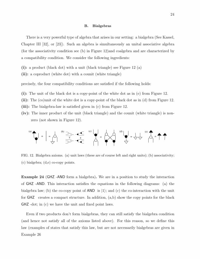
(i): a product (black dot) with a unit (black triangle) see Figure 12 (a)
(ii): a coproduct (white dot) with a counit (white triangle)
precisely, the four compatibility conditions are satisfied if the following holds:
(i): The unit of the black dot is a copy-point of the white dot as in (e) from Figure 12.
(ii): The (co)unit of the white dot is a copy-point of the black dot as in (d) from Figure 12.
(iii): The bialgebra-law is satisfied given in (c) from Figure 12.
(iv): The inner product of the unit (black triangle) and the counit (white triangle) is non-
zero (not shown in Figure 12).
= = ==
(a) (d)(c)
=
(b) (e)= =
FIG. 12. Bialgebra axioms. (a) unit laws (these are of course left and right units); (b) associativity;
(c) bialgebra; (d,e) co-copy points.
Example 24 (GHZ -AND form a bialgebra). We are in a position to study the interaction
of GHZ -AND. This interaction satisfies the equations in the following diagrams: (a) the
bialgebra law; (b) the co-copy point of AND is |1〉; and (c) the co-interaction with the unit
for GHZ creates a compact structure. In addition, (a,b) show the copy points for the black
GHZ -dot; in (c) we have the unit and fixed point laws.
Even if two products don’t form bialgebras, they can still satisfy the bialgebra condition
(and hence not satisfy all of the axioms listed above). For this reason, so we define this
law (examples of states that satisfy this law, but are not necessarily bialgebras are given in
Example 26
25
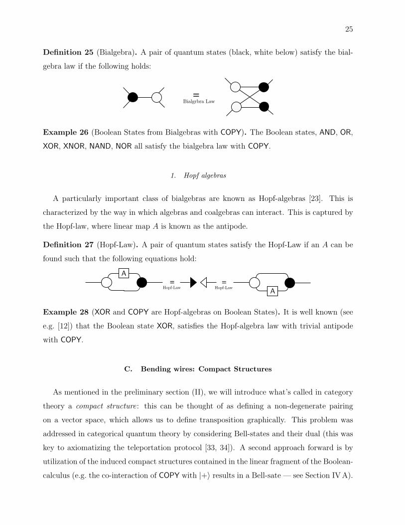
Definition 25 (Bialgebra). A pair of quantum states (black, white below) satisfy the bial-
gebra law if the following holds:
=
Example 26 (Boolean States from Bialgebras with COPY). The Boolean states, AND, OR,
XOR, XNOR, NAND, NOR all satisfy the bialgebra law with COPY.
1. Hopf algebras
A particularly important class of bialgebras are known as Hopf-algebras [23]. This is
characterized by the way in which algebras and coalgebras can interact. This is captured by
the Hopf-law, where linear map A is known as the antipode.
Definition 27 (Hopf-Law). A pair of quantum states satisfy the Hopf-Law if an A can be
found such that the following equations hold:
= =
Example 28 (XOR and COPY are Hopf-algebras on Boolean States). It is well known (see
e.g. [12]) that the Boolean state XOR, satisfies the Hopf-algebra law with trivial antipode
with COPY.
C. Bending wires: Compact Structures
As mentioned in the preliminary section (II), we will introduce what’s called in category
theory a compact structure: this can be thought of as defining a non-degenerate pairing
on a vector space, which allows us to define transposition graphically. This problem was
addressed in categorical quantum theory by considering Bell-states and their dual (this was
key to axiomatizing the teleportation protocol [33, 34]). A second approach forward is by
utilization of the induced compact structures contained in the linear fragment of the Boolean-
calculus (e.g. the co-interaction of COPY with |+〉 results in a Bell-sate — see Section IVA).

26
A compact structure on an object H consists of another object H∗ together with a pair
of morphisms (note that we use the equation H∗ = H in Hilbert space making objects self
dual which simplifies what follows).
ηH : 1 −→ H⊗H εH : H⊗H −→ 1
where the canonical representation in Hilbert space with dimension N and basis {|i〉} is
given by
ηH =N∑i=1
|i〉 ⊗ |i〉 εH =N∑i=1
〈i| ⊗ 〈i|
and in string diagrams (read from the top to the bottom of the page) as
(a) (b)time
These cups and caps give rise to cup/cap-induced duality: this amounts to being able to
create a linear map that “flips” a bra to a ket (and vise versa) and at the same time taking
an (anti-linear) complex conjugate. Under cup/cap-induced duality, we flip the second ket
on ηH and the first bra on εH to relate these maps and the identity 1H of the Hilbert space:
that is, we can fix a basis and construct invertible maps sending ηH w 1H w εH.
More generally, the maps ηH and εH satisfy the following equations and their duals (under
the dagger) in the graphical language (b is known as the snake equation).
=
=
(a)
(b)f
fT
=
=�
�‒
= f
(c)
(d)
Definition 29 (Diagrammatic Adjoints). Cups and caps allow us to take the transpose of
a linear map (b); and (a) following [16] we introduce the derived concept of adjoint.
=(a) (b)
=

27
VI. TRANSLATING ANY QUANTUM STATE INTO A CATEGORICAL
TENSOR NETWORK
Typically only the converse is possible — that is, one determines a quantum state from
a given tensor network or quantum circuit, or perhaps performs an optimization or renor-
malization procedure over a set of network parameters to find the network representing the
state that best e.g. minimizes a given Hamiltonian. While tensor networks are in theory
expressive enough to represent any quantum state, doing so will typically not expose ad-
ditional internal structure (see the general from of a Matrix Product State in Figure 13).
On the other hand, our new methods enable one to translate a quantum state directly into
a new type of network: a so-called categorical tensor network. We have already presented
the algebraic definitions and and defining properties of these new components. Here we will
illustrate their expressive power by considering a few elementary examples before presenting
our main theorem (35).
A. Extending the State of the Art
Tensor network states are in wide spread current use (see the reviews [5, 24]). The current
approach does not expose much internal structure of the constituent tensors comprising a
given network. Indeed, all MPS states have essentially the same topological or network struc-
ture in the current incarnation (see Figure 13). There is however, ample internal structure
to exploit. The current approach to write down a matrix product state is ad hoc and via
trial and error. For instance, the current approach shows little insight into why the W-state
on n-qubits takes the form:
Wn = 〈0|
|0〉 0
|1〉 |0〉
n
|1〉 = |10...0〉+ |01...0〉+ ...+ |00...1〉 (30)
or importantly, how to arrive at a tensor network for more complicated states. We will build
on a specific example, and show how our alternative approach reveals new found internal
structure when representing quantum states in terms of a network.

28
FIG. 13. W-state on n-parties in the Matrix Product State formalism in wide spread current use
(see (30)). Note that the internal structure of the tensors themselves can not be exposed in the
current formalism: all states in this formalism have this same topological structure.
B. Example: W-states in the Categorical Tensor Network Formalism
W-states can arise in our framework in several ways. To help build a feeling for the general
setting, consider the following:
Example 30 (Functions onW- and GHZ -states). We consider the function fW which outputs
logical-one given input bit string 001, 010 and 100 and logical-zero otherwise. Likewise the
function fGHZ is defined to output logical-one on input bit strings 000 and 111 and logical-
zero otherwise. See Examples (32) and (33) which consider representation of these functions
as polynomials. We will of course continue to work with a linear representation of quantum
states, where bit string 000 7→ |000〉 (etc.).
Remark 31 (Exact-value functions). The function fW takes value one on input vectors with
k ones for a fixed k. Such functions are known in the literature as a Exact-value symmetric
Boolean functions.
Example 32 (Function Realisation of fW and fGHZ: the Boolean case). One can express
fW(x1, x2, x3) = x1x2x3 ⊕ x1x2x3 ⊕ x1x2x3 (31)
by noting that each term in the disjunctive normal form of fW are disjoint, and hence ∨ 7→ ⊕.
The algebraic normal form (see Appendix A) becomes
fW(x1, x2, x3) = x1 ⊕ x2 ⊕ x3 ⊕ x1x2x3 (32)
fGHZ(x1, x2, x3) = 1⊕ x1 ⊕ x2 ⊕ x3 ⊕ x1x2 ⊕ x1x3 ⊕ x2x3 (33)
Example 33 (Function Realisation of fW and fGHZ: the set function case). Set functions
are mappings from the family of subsets of a finite ground set (e.g. Booleans) to the set of

29
reals. In the Circuit Theory literature, functions from the Booleans to the reals are known as
pseudo-Boolean functions and more commonly as multi-linear polynomials or forms (see [18]
where these functions are used to embed logic gates in the ground state energy configuration
of spin models). Their exists a unique multi-linear polynomial representation for each pseudo-
Boolean function found by mapping the negated Boolean variable as x 7→ (1 − x). For the
GHZ - and W-functions defined in Example 30 we arrive at the unique polynomials (33) and
(33).
fGHZ(x1, x2, x3) = 1− x1 − x2 + x1x2 − x3 + x1x3 + x2x3 (34)
fW(x1, x2, x3) = x1 + x2 + x3 − 2x1x2 − 2x1x3 − 2x2x3 + 3x1x2x3 (35)
These polynomials (33) and (33) are readily translated into categorical tensor networks.
Example 34 (Network realisation of W- and GHZ -states). A network realization of W-
and GHZ -states in our framework then follows by post-selecting to |1〉 on the output bit —
leaving the input qubits to represent a W- or GHZ -state respectively. As example of this is
shown in Figure 14.
=
tim
e
(a) (b)
=
time
FIG. 14. Left (a) the circuit realisation (internal to the triangle) of the function fW of e.g. (32)
which outputs logical-one given input bit string |x1x2x3〉 = |001〉, |010〉 and |100〉 and logical-
zero otherwise. Right (b) reversing time and setting the output to |1〉 (e.g. post-selection) gives a
network representing the W-state. See also Figure 15.
C. The General Case
A starting point of the classical network theory was seminal work resulting in Shannon
and Davio decompositions of functions into networks. These powerful methods formed the
30
= =
(a) (b)
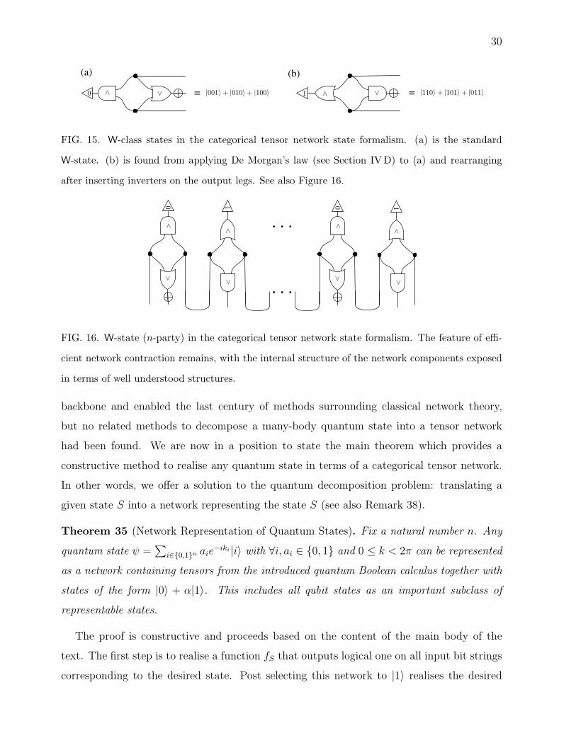
FIG. 15. W-class states in the categorical tensor network state formalism. (a) is the standard
W-state. (b) is found from applying De Morgan’s law (see Section IVD) to (a) and rearranging
after inserting inverters on the output legs. See also Figure 16.
FIG. 16. W-state (n-party) in the categorical tensor network state formalism. The feature of effi-
cient network contraction remains, with the internal structure of the network components exposed
in terms of well understood structures.
backbone and enabled the last century of methods surrounding classical network theory,
but no related methods to decompose a many-body quantum state into a tensor network
had been found. We are now in a position to state the main theorem which provides a
constructive method to realise any quantum state in terms of a categorical tensor network.
In other words, we offer a solution to the quantum decomposition problem: translating a
given state S into a network representing the state S (see also Remark 38).
Theorem 35 (Network Representation of Quantum States). Fix a natural number n. Any
quantum state ψ =∑
i∈{0,1}n aie−iki|i〉 with ∀i, ai ∈ {0, 1} and 0 ≤ k < 2π can be represented
as a network containing tensors from the introduced quantum Boolean calculus together with
states of the form |0〉 + α|1〉. This includes all qubit states as an important subclass of
representable states.
The proof is constructive and proceeds based on the content of the main body of the
text. The first step is to realise a function fS that outputs logical one on all input bit strings
corresponding to the desired state. Post selecting this network to |1〉 realises the desired

31
superposition of terms, but with all coefficients and hence relative phases equal. To adjust
the phases and relative amplitudes, we will construct diagonal operators. Given a term |k〉
in a state, with coefficient αk, we construct a function fd that outputs local zero for all
inputs not equal to k, and logical one for input k. The network is then post selected to
|0〉+αk|1〉 and we transform fd into an operator by using COPY-dots from Section IVE (see
Figure 17 and Example 36). We note that the construction can be improved significantly
by considering several reductions. We of course group terms in the state with the same
coefficients αi, but further reductions are also possible if say a given set of coffecients are
given by products of other coffecients. This is illustrated by networks that take the form
=
time
... ... ......
where we note that the fan-in present in the networks, can result in networks that are not
thought to be efficiently contactable. In addition, each of these networks gives a prescription
to physically prepare a state, however when fan-in is present, this prescription does not
represent a deterministic process (see Corollary 42).
Example 36 (Network realisation of S = |01〉+ |10〉+α|11〉). As a simple example, we will
design a network to realise the state |01〉 + |10〉 + α|11〉. We first write down a function fS
such that
fS(0, 1) = fS(1, 0) = fS(1, 1) = 1 (36)
and fS(00) = 0 (in this case, fS is the logical OR-gate). We post select the network on |1〉,
which results in the state |01〉+ |10〉+α|11〉, see Figure 17 (a). The next step is to realise a
diagonal operator, that acts on identity on all inputs, except |11〉 which gets sent to α|11〉.
To do this, we design a function fd such that
fd(0, 1) = fd(1, 0) = fd(0, 0) = 0 (37)
32
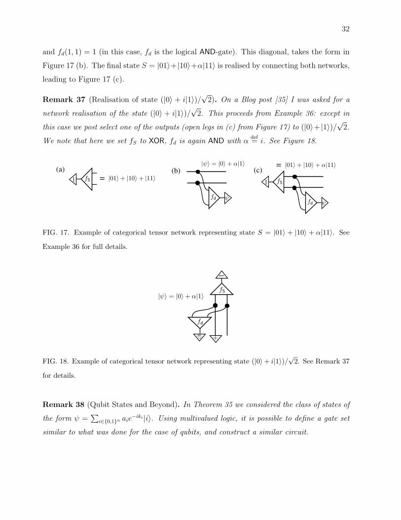
and fd(1, 1) = 1 (in this case, fd is the logical AND-gate). This diagonal, takes the form in
Figure 17 (b). The final state S = |01〉+ |10〉+α|11〉 is realised by connecting both networks,
leading to Figure 17 (c).
Remark 37 (Realisation of state (|0〉 + i|1〉)/√2). On a Blog post [35] I was asked for a
network realisation of the state (|0〉 + i|1〉)/√2. This proceeds from Example 36: except in
this case we post select one of the outputs (open legs in (c) from Figure 17) to (|0〉+ |1〉)/√2.
We note that here we set fS to XOR, fd is again AND with αdef= i. See Figure 18.
(a) (b)=
=(c)
FIG. 17. Example of categorical tensor network representing state S = |01〉 + |10〉 + α|11〉. See
Example 36 for full details.
FIG. 18. Example of categorical tensor network representing state (|0〉+ i|1〉)/√2. See Remark 37
for details.
Remark 38 (Qubit States and Beyond). In Theorem 35 we considered the class of states of
the form ψ =∑
i∈{0,1}n aie−iki|i〉. Using multivalued logic, it is possible to define a gate set
similar to what was done for the case of qubits, and construct a similar circuit.

33
D. Categorical MERA Networks and Solving SAT instances
In the previous sections we developed a powerful framework — we can use it to make
seemingly daunting calculations elementary. As a token of the power, we will now consider
examples of the presented calculus applied to a categorical description of a MERA network
and then in VIF explain how our approach enables a rang of classical optimization problems
(such as SAT) to be addressed by tensor contraction.
E. Categorical MERA Networks
The Multi-scale Entanglement Renormalization Ansatz (MERA) approach is a combina-
tion of the seminal ideas of Kadanoff’s spin-blocking, Wilson’s real-space renormalization
and White’s DMRG procedure. Renormalization proceeds by coarse-graining lattice sites
and truncating the description. DMRG’s success is based on properly identifying the opti-
mal truncation. The key feature of MERA is that it dramatically reduces information loss
due to truncation by eliminating entanglement beforehand [4]. Repeating this entanglement
renormalization procedure generates a hierarchical network, (shown below), where entangle-
ment at different length scales is efficiently described. Within this structure the properties
of quantum critical systems and emergent quantum phenomena are known to be efficiently
computable.
In numerical algorithms, it is desirable to calculate correlation functions from the above
network. We are interested in comparing quantities such as < xixj > and < xi >< xj >.
We can leverage our calculus to complete this task by noting that:
34
(⊕-dots): These dots are Hadamard transforms of the black COPY-dots and hence satisfy
the evident algebraic properties: (i) the spider law (Theorem 22) and so can be merged
into a single dot; (ii) they form a bialgebra with COPY-dots (Section VB); (iii) they
satisfy the Hopf-Law (with trivial antipode — Section VB); (iv) the unit of the ⊕-dot
is |0〉 and its co-unit interaction leads to the familiar compact structure.
(•-dots): These are the COPY-dots we have considered in Sections IVA and IVE which
have all the same properties as above, with unit |+〉.
(AND-dots): AND-dots where defined in Section IVD. These dots correspond to quantum
states that are outside the stabilizer class and, as mentioned, have the following alge-
braic properties: (i) form bialgebras with COPY-dots; (ii) have unit |1〉; (iii) co-unit
interaction that results in a copy-point; (iv) have a fixed point (|0〉); (v) as the dots
form an associative algebra, there is no ambiguity in their merger.
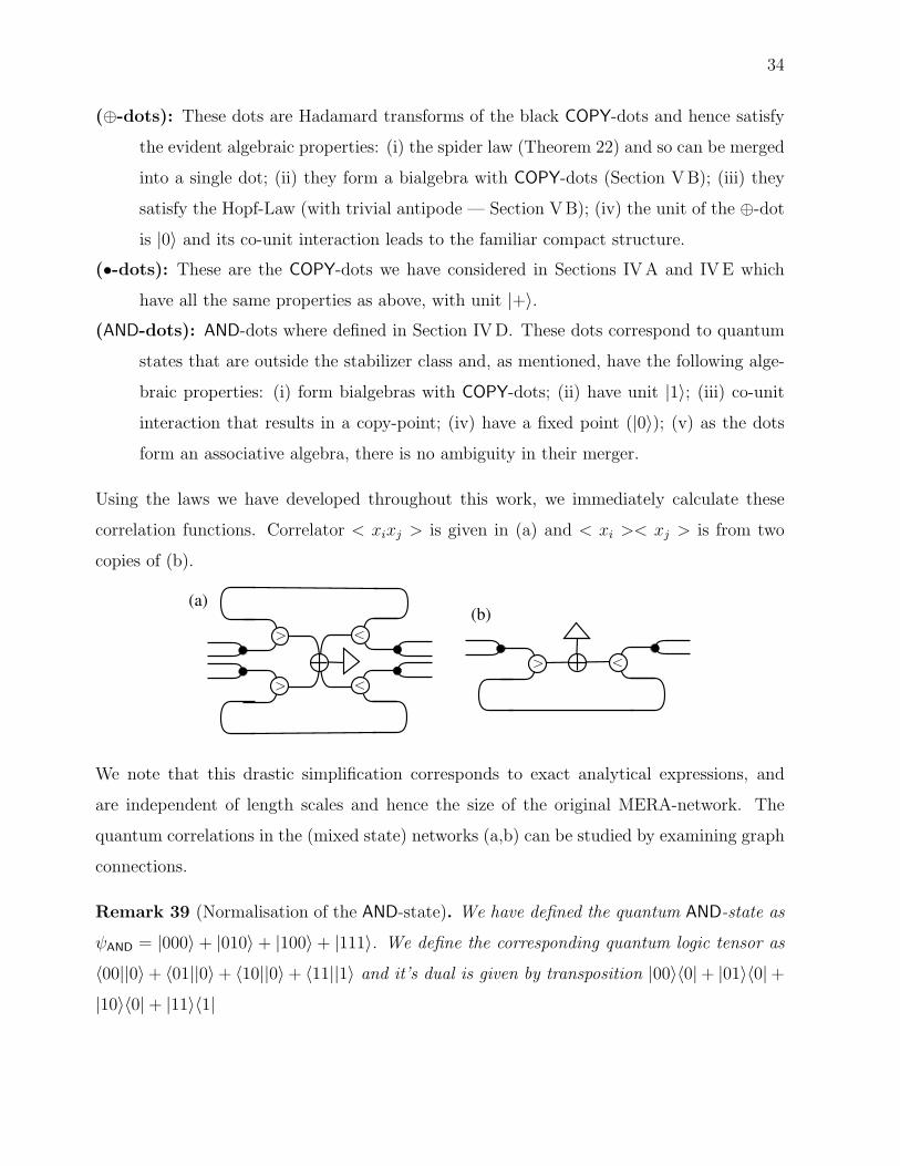
Using the laws we have developed throughout this work, we immediately calculate these
correlation functions. Correlator < xixj > is given in (a) and < xi >< xj > is from two
copies of (b).
(a)(b)
We note that this drastic simplification corresponds to exact analytical expressions, and
are independent of length scales and hence the size of the original MERA-network. The
quantum correlations in the (mixed state) networks (a,b) can be studied by examining graph
connections.
Remark 39 (Normalisation of the AND-state). We have defined the quantum AND-state as
ψAND = |000〉 + |010〉 + |100〉 + |111〉. We define the corresponding quantum logic tensor as
〈00||0〉+ 〈01||0〉+ 〈10||0〉+ 〈11||1〉 and it’s dual is given by transposition |00〉〈0|+ |01〉〈0|+
|10〉〈0|+ |11〉〈1|

35
F. SAT and read-once formula
In future work with Stephen Clark and Dieter Jaksch, we will study in detail how the
presented calculus enables one to address Satisfiability and other related problems in terms
of a network contraction. Indeed, the method leads immediately to a method to contract
a function representing a SAT-instance: e.g. if the contraction results in scalar zero, the
function represents a NO instance. See Figure 19.
=
tim
e
(a) (b)
...
...
FIG. 19. Solving NP-complete problems by contracting a the Categorical Tensor Network. (a) A
SAT-formula realised as a network. (b) contracting the network: if this contraction evaluates to
one the SAT instance is satisfiable and if it evaluates to zero it is not.
Remark 40 (MERA and read-once Boolean formula). The class of Boolean networks that
only allow fan-in (e.g. no bit merging) are known as read-once formula or networks. MERA
is a quantum version of this class (see also Table 20).
Corollary 41 (All read-once formula are SAT YES instances). Using the method described
above for SAT (See Figure 19) it immediately follows that all read-once formula are satisfi-
able.
Corollary 42 (A prescription to realize any read-once quantum state deterministically).
We call the class of read-once Boolean quantum states as those states prepared by read-
once binary networks as given in Figure 14 where fW is a read-once formula and hence
the network generates states encoding the constraint fW = 1 (see Example 30). If fW is a
read-once formula, it corresponds to a fanout only quantum network, and hence this network
represents a deterministic process to realize the physical state corresponding to fW . This
extends to the evident way to quantum read-once states which are exactly the MERA class.
See [17, 20] for more details.

36
VII. OUTLOOK AND CONCLUDING REMARKS
We have presented a solution to the quantum decomposition problem based on a rep-
resentation of quantum states in terms of categorical tensor networks. The expressiveness
and power of this new method was illustrated by considering several test cases: we unveiled
hidden internal structure of MPS states (e.g. W-states) and illustrated the simplification
power of these methods by considering our example applied to MERA-networks. We have
opened up many future potential research directions. For instance, our methods now readily
allow tensor network algorithms (which work by contracting tensors) to solve NP-complete
problems. We conclude by presenting a table (20) which summarizes some of the mathe-
matical structures that are already present in the tensor networks community (and their
corresponding Categories) as well as some mathematical structures that arise as categorical
tensor networks. I have plans to take this aspect of this work further in joint work with John
Baez [21, 35].
Categories Fan-in and Fan-out Only Fan-in
Many Types Symmetric Monoidal Category [14, 36] Symmetric Multicategory
One Type PROP [37] Operad
Switching Networks Fan-in and Fan-out Only Fan-in
Many Types General Switching Networks General Read-once formula
One Type General Boolean Networks [25] Read-once Boolean circuits
Tensor Networks Fan-in and Fan-out Only Fan-in
Many Types Categorical Tensor Networks Tree Tensor Networks
One Type ? MERA Networks
FIG. 20. Table illustrating how the symmetric categories of interest fit together and their cor-
responding classical network, and tensor network. See also the related non-symmetric categories
listed in Table 21.
37
ACKNOWLEDGMENTS
We thank John Baez, Stephen Clark, Dieter Jaksch and Mike Shulman. JDB received
support from EPSRC grant EP/G003017/1 and completed large parts of this work visiting
the Center for Quantum Technologies, at the National University of Singapore (these visits
were hosted by Vlatko Vedral).
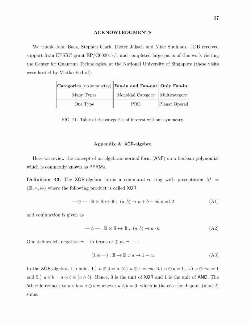
Categories (no symmetry) Fan-in and Fan-out Only Fan-in
Many Types Monoidal Category Multicategory
One Type PRO Planar Operad
FIG. 21. Table of the categories of interest without symmetry.
Appendix A: XOR-algebra
Here we review the concept of an algebraic normal form (ANF) on a boolean polynomial
which is commonly known as PPRMs.
Definition 43. The XOR-algebra forms a commutative ring with presentation M =
{B,∧,⊕} where the following product is called XOR
—⊕— : B× B 7→ B :: (a, b) → a+ b− ab mod 2 (A1)
and conjunction is given as
— ∧— : B× B 7→ B :: (a, b) → a · b. (A2)
One defines left negation ¬— in terms of ⊕ as ¬— ≡
(1⊕—) : B 7→ B :: a→ 1− a. (A3)
In the XOR-algebra, 1-5 hold. 1.) a⊕ 0 = a, 2.) a⊕ 1 = ¬a, 3.) a⊕ a = 0, 4.) a⊕ ¬a = 1
and 5.) a ∨ b = a⊕ b⊕ (a ∧ b). Hence, 0 is the unit of XOR and 1 is the unit of AND. The
5th rule reduces to a ∨ b = a⊕ b whenever a ∧ b = 0, which is the case for disjoint (mod 2)
sums.

38
Definition 44. Any boolean equation may be uniquely expanded to the fixed polarity Reed-
Muller form as:
f(x1, x2, ..., xk) = c0 ⊕ c1xσ11 ⊕ c2x
σ22 ⊕ · · · ⊕ cnx
σnn ⊕
cn+1xσ11 x
σnn ⊕ · · · ⊕ c2k−1x
σ11 x
σ22 , ..., x
σkk , (A4)
where selection variable σi ∈ {0, 1}, literal xσii represents a variable or its negation and any
c term labeled c0 through cj is a binary constant 0 or 1. In Equation A4 only fixed polarity
variables appear such that each is in either un-complemented or complemented form.
Let us now consider derivation of the form from Definition 44. Because of the structure
of the algebra, without loss of generality, one avoids keeping track of indices in the N node
case, by considering the case where N ≡ 2n = 8.
Example 45. The vector c = (c0, c1, c2, c3, c4, c5, c6, c7, )ᵀ represents all possible outputs of
any function f(x1, x2, x3) over the algebra formed from linear extension of Z2×Z2×Z2. We
wish to construct a canonical representation in terms of the vector c, where each ci ∈ {0, 1},
and therefore c is a selection vector that simply represents the output of the function f :
B× B× B → B :: (x1, x2, x3) 7→ f(x1, x2, x3). One may expand f as:
f(x1, x2, x3) = (c0 · ¬x1 · ¬x2 · ¬x3) ∨ (c1 · ¬x1 · ¬x2 · x3) ∨ (c2 · ¬x1 · x2 · ¬x3)
∨(c3 · ¬x1 · x2 · x3) ∨ (c4 · x1 · ¬x2 · ¬x3) ∨ (c5 · x1 · ¬x2 · x3)
∨(c6 · x1 · x2 · ¬x3) ∨ (c7 · x1 · x2 · x3) (A5)
Since each disjunctive term is disjoint the logical OR operation can be replaced with
the logical XOR operation. By making the substitution ¬a = a ⊕ 1 for all variables and
rearranging terms one arrives at the following canonical form:1
f(x1, x2, x3) = c0 ⊕ (c0 ⊕ c4) · x1 ⊕ (c0 ⊕ c2) · x2 ⊕ (c0 ⊕ c1) · x3 ⊕ (c0 ⊕ c2 ⊕ c4 ⊕ c6) · x1 · x2
⊕(c0 ⊕ c1 ⊕ c4 ⊕ c5) · x1 · x3 ⊕ (c0 ⊕ c1 ⊕ c2 ⊕ c3) · x2 · x3
⊕(c0 ⊕ c1 ⊕ c2 ⊕ c3 ⊕ c4 ⊕ c5 ⊕ c6 ⊕ c7) · x1 · x2 · x3 (A6)
1 For instance, ¬x1 · ¬x2 · ¬x3 = (1 ⊕ x1) · (1 ⊕ x2) · (1 ⊕ x3) = (1 ⊕ x1 ⊕ x2 ⊕ x2 · x3) · (1 ⊕ x3) =
1⊕ x1 ⊕ x2 ⊕ x3 ⊕ x1 · x3 ⊕ x2 · x3 ⊕ x1 · x2 · x3.

39
The set of linearly independent vectors, {x1, x2, x3, x1·x2, x1·x3, x2·x3, x1·x2·x3} combined
with a set of scalars from Equation A6 spans the eight dimensional space of the Hypercube
representing the Algebra. A similar form holds for arbitrary N .
f(x1, x2, x3) = (a1) · x1 ⊕ (a2) · x2 ⊕ (x3) · x3 ⊕ (a1 ⊕ a2 ⊕ a1 ⊕ c2) · x1 · x2
⊕(a1 ⊕ a3 ⊕ a1 ⊕ c3) · x1 · x3 ⊕ (a2 ⊕ a3 ⊕ a2 ⊕ c3) · x2 · x3
⊕(a1 ⊕ a2 ⊕ a3 ⊕ a1 ⊕ a2 ⊕ a3) · x1 · x2 · x3 (A7)
Example 46. The Galois group: of every finite field extension of a finite field is finite and
cyclic; conversely, given a finite field F and a finite cyclic group G, there is a finite field
extension of F whose Galois group is G.
[1] Saunders Mac Lane. Categories for the working mathematician 2nd ed. Graduate Texts in
Mathematics, Springer, 1998.
[2] Steven R. White. Density matrix formulation for quantum renormalization groups. Phys. Rev.
Lett., 69(19):2863–2866, Nov 1992.
[3] A. Aspuru-Guzik and Jr. W. A. Lester. Quantum monte carlo methods for the solution of the
schroedinger equation for molecular systems. Handbook of Numerical Analysis, X, 2003.
[4] G. Vidal. Class of Quantum Many-Body States That Can Be Efficiently Simulated. Physical
Review Letters, 101(11):110501, 2008.
[5] F. Verstraete, V. Murg, and J. I. Cirac. Matrix product states, projected entangled pair
states, and variational renormalization group methods for quantum spin systems. Advances
in Physics, 57:143–224, 2008.
[6] G. Vidal. Efficient classical simulation of slightly entangled quantum computations. Phys.
Rev. Lett., 91:147902, 2003.
[7] G. Vidal. Efficient simulation of one-dimensional quantum many-body systems. Phys. Rev.
Lett., 93:040502, 2004.
[8] Jacob Biamonte, Stephen Clark, Mark Williamson, and Vlatko Vedral. The Quan-

40
tum Theory of Information and Computation. Oxford Graduate Course, TT2010.
www.comlab.ox.ac.uk/activities/quantum/course/.
[9] T. H. Johnson, S. R. Clark, and D. Jaksch. Dynamical simulations of classical stochastic
systems using matrix product states. Phys. Rev. E, 82(3):036702, Sep 2010.
[10] J. C. Baez and M. Stay. Physics, Topology, Logic and Computation: A Rosetta Stone. ArXiv
e-prints, March 2009.
[11] J. C. Baez and A. Lauda. A Prehistory of n-Categorical Physics. ArXiv e-prints, August 2009.
[12] Yves Lafont. Towards an algebraic theory of boolean circuits. Journal of Pure and Applied
Algebra, 184:2003, 2003.
[13] Y. Guiraud. The three dimensions of proofs. ArXiv Mathematics e-prints, December 2006.
[14] A. Joyal and R. Street. The geometry of tensor calculus i. Advances in Mathematics, 88(55),
1991.
[15] P. Selinger. A survey of graphical languages for monoidal categories. ArXiv e-prints, August
2009.
[16] Samson Abramsky and Bob Coecke. Categorical quantum mechanics. Chapter in the Handbook
of Quantum Logic and Quantum Structures vol II, Elsevier, 2008.
[17] Jacob D Biamonte. Categorical models of quantum circuits. Technical Report RR-10-05,
OUCL, May 12th 2010.
[18] J. D. Biamonte. Nonperturbative k -body to two-body commuting conversion Hamiltonians
and embedding problem instances into Ising spins. Phys. Rev. A , 77(5):052331, May 2008.
[19] Peter Selinger. Dagger compact closed categories and completely positive maps: (extended
abstract). Electronic Notes in Theoretical Computer Science, 170:139 – 163, 2007. Proceedings
of the 3rd International Workshop on Quantum Programming Languages (QPL 2005).
[20] Jacob Biamonte and Ville Bergholm. Categorical quantum circuits. Technical Report RR-10-
17, OUCL, Sep 28th 2010.
[21] John Baez et al. Bimonoids from biproducts. The n-Category Cafe Blog. online
at: http://golem.ph.utexas.edu/category/2010/09/bimonoids from biproducts.html.
[22] Bob Coecke and Ross Duncan. Interacting quantum observables: Categorical algebra and
diagrammatics. aXriv preprint 0906.4725, 2009.
[23] Joachim Kock. Frobenius algebras and 2-d topological quantum field theories. Cambridge

41
University Press, 2003.
[24] J. I. Cirac and F. Verstraete. Renormalization and tensor product states in spin chains and
lattices. J. Phys. A Math. Gen., 42:4004, 2009.
[25] I. Wegener. The complexity of boolean functions. Wiley-Teubner, 1987. online
at: http://eccc.hpi-web.de/.
[26] E. Boros and P.L. Hammer. Pseudo-boolean optimization. Discrete Applied Mathematics,
123(1-3):155–225, 2002.
[27] A. Kitaev, A. Shen, and M. Vyalyi. Classical and quantum computation. AMS, Graduate
Studies in Mathematics, 47, 2002.
[28] Michael Nielsen and Isaac Chuang. Quantum computation and quantum information. Cam-
bridge University Press, 2000.
[29] B. Coecke, D. Pavlovic, and J. Vicary. A new description of orthogonal bases. ArXiv e-prints,
October 2008.
[30] D. Aharonov. A simple proof that toffoli and hadamard are quantum universal. 2003.
quant-ph/0301040.
[31] Roger Penrose. Applications of negative dimensional tensors. Combinatorial Mathematics and
its Applications, Academic Press, 1971.
[32] C. Kassel. Quantum groups. Springer Graduate Texts in Mathematics, 1994.
[33] Samson Abramsky and Bob Coecke. A categorical semantics of quantum protocols. Proceedings
of the 19th IEEE conference on Logic in Computer Science (LiCS’04), 2004.
[34] B. Coecke. Kindergarten Quantum Mechanics. ArXiv Quantum Physics e-prints, October
2005.
[35] John Baez et al. Jacob biamonte on tensor networks. The n-Category Cafe Blog. online
at: http://golem.ph.utexas.edu/category/2010/09/jacob biamonte on tensor netwo.html.
[36] Max Kelly and M. L. Laplaza. Coherence for compact closed categories. Journal of Pure and
Applied Algebra, 19:193–213, 1980.
[37] S. Mac Lane. Categorical algebra. Bull. Amer. Math. Soc., 71, 1965.