temperature, salinity, density, and the oceanic pressure field

pdf version 1.0 (December 2001)

Chapter 2

Temperature, salinity, density, and the oceanic pressure field

The ratios of the many components which make up the salt in the ocean are remarkablyconstant, and salinity, the total salt content of seawater, is a well-defined quantity. For awater sample of known temperature and pressure it can be determined by only onemeasurement, that of conductivity.

Today, the single most useful instrument for oceanographic measurements is the CTD,which stands for "Conductivity-Temperature-Depth". It is sometimes also known as theSTD, which stands for "Salinity-Temperature-Depth"; but CTD is the more accuratedescription, because in both systems salinity is not directly measured but determinedthrough a conductivity measurement. Even the term CTD is inaccurate, since depth is adistance, and a CTD does not measure its distance from the sea surface but employs apressure measurement to indicate depth. But the three most important oceanographicparameters which form the basis of a regional description of the ocean are temperature,salinity, and pressure, which the CTD delivers.

In this text we follow oceanographic convention and express temperature T and potentialtemperature Θ in degrees Celsius (°C) and pressure p in kiloPascal (kPa, 10 kPa = 1 dbar,0.1 kPa = 1 mbar; for most applications, pressure is proportional to depth, with 10 kPaequivalent to 1 m). Salinity S is taken to be evaluated on the Practical Salinity Scale (evenwhen data are taken from the older literature) and therefore carries no units. Density ρ isexpressed in kg m-3 or represented by σt = ρ - 1000. As is common oceanographicpractice, σt does not carry units (although strictly speaking it should be expressed inkg m-3 as well). Readers not familiar with these concepts should consult textbooks such asPickard and Emery (1990), Pond and Pickard (1983), or Gill (1982); the last two includeinformation on the Practical Salinity Scale and the Equation of State of Seawater whichgives density as a function of temperature, salinity, and pressure. We use z for depth(z being the vertical coordinate in a Cartesian xyz coordinate system with x pointing eastand y pointing north) and count z positive downward from the undisturbed sea surfacez = 0 .

A CTD typically returns temperature to 0.003°C, salinity to 0.003 parts per thousand,and depth to an accuracy of 1 - 2 m. Depth resolution can be much better, and advancedCTD systems, which produce data triplets at rates of 20 Hz or more and apply dataaveraging, give very accurate pictures of the structure of the ocean along a vertical line. Thebasic CTD data set, called a CTD station or cast, consists of continuous profiles oftemperature and salinity against depth (Figure 2.1 shows an example). The task of anoceanographic cruise for the purpose of regional oceanography is to obtain sufficient CTDstations over the region of interest to enable the researcher to develop a three-dimensionalpicture of these parameters and their variations in time. As we shall see later, such a dataset generally gives a useful picture of the velocity field as well.

For a description of the world ocean it is necessary to combine observations from manysuch cruises, which is only possible if all oceanographic institutions calibrate theirinstrumentation against the same standard. The electrical sensors employed in CTD systemsdo not have the long-term stability required for this task and have to be routinely calibratedagainst measurements obtained with precision reversing thermometers and with

Regional Oceanography: an Introduction


16

salinometers, which compare water samples from CTD stations with a seawater standard ofknown salinity (for details see Dietrich et al., 1980). A CTD is therefore usually housed

Fig. 2.2. A CTD is retrieved after completion of a station. The instrument is mounted in thelower centre, protected by a metal cage to prevent damage in rough weather. Above the CTD are24 sampling bottles for the collection of water samples. The white plastic frames attached tosome of them carry precision reversing thermometers.

Fig. 2.1.

An example of the basic CTDdata set. Temperature T andsalinity S are shown againstpressure converted to depth.Also shown is the derivedquantity σt.


The oceanic pressure field 17

inside a frame, with 12 or more bottles around it (Figure 2.2). The water samples collectedin the bottles are used for calibration of the CTD sensors. In addition, oxygen and nutrientcontent of the water can be determined from the samples in the vessel's laboratory.

The CTD developed from a prototype built in Australia in the 1950s and has been amajor tool of oceanography at the large research institutions since the 1970s. Two decadesare not enough to explore the world ocean fully, and regional oceanography still has to relyon much information gathered through bottle casts, which produce 12 - 24 samples overthe entire observation depth and therefore are of much lower vertical resolution. Althoughbottle data have been collected for nearly 100 years now, significant data gaps still exist, asis evident from the distribution of oceanographic stations shown in Figure 2.3. In the deepbasins of the oceans, where variations of temperature and salinity are small, very high dataaccuracy is required to allow integration of data from different cruises into a single data set.Many cruise data which are quite adequate for an oceanographic study of regional importanceturn out to be inadequate for inclusion in a world data set.

To close existing gaps and monitor long-term changes in regions of adequate datacoverage, a major experiment, planned for the decade 1990 - 2000, is under way. ThisWorld Ocean Circulation Experiment (WOCE) will cover the world ocean with a networkof CTD stations, extending from the surface to the ocean floor and including chemicalmeasurements. Figure 2.4 shows the planned global network of cruise tracks along whichCTD stations will be made at intervals of 30 nautical miles (half a degree of latitude, orabout 55 km). As a result, we can expect to have a very accurate global picture of thedistribution of the major oceanographic parameters by the turn of the century.

Because of the need for a global description of the oceanic parameter fields, researchershave attempted to extract whatever information they can from the existing data base.

Fig. 2.3. World wide distribution of oceanographic stations of high data quality shortly before1980. Unshaded 5° squares contain at least one high-quality deep station. Shaded 5° squarescontain at least one high-quality station in a shallow area. Black 5° squares contain no high-quality station. Adapted from Worthington (1981)



18

Fig. 2.4. The hydrographic sections of the World Ocean Circulation Experiment (WOCE).Shaded regions indicate intensive study areas. Dots indicate positions of current metermoorings.

Figure 2.5 is an example of a recent and widely used attempt. It includes all availableoceanographic data regardless of absolute accuracy and shows that many features of theoceans can be studied without the very high data accuracy required for the analysis of thedeep basins. Features such as the large pool of very warm surface water in the equatorialwestern Pacific and eastern Indian Oceans, the outflow of high salinity water from theEurafrican Mediterranean Sea into the Atlantic Ocean below 1000 m depth, the formation ofcold bottom water in the Weddell and Ross Seas near Antarctica, or the outflow of lowsalinity water from the Indonesian seas into the Indian Ocean, are all clearly visible in theexisting data base. However, it should be remembered that the number of observationsavailable for every 2° square varies considerably over the area and decreases quickly with

Fig. 2.5 (pages 19 – 21). Climatological mean potential temperature Θ (°C) and salinity S forthe world ocean. Page 19: (a) Θ at z = 0 m, (b) S at z = 0 m, Page 20: (c) Θ at z = 5 0 0 m ,(d) S at z = 500 m, Page 21: (e) Θ at z = 2000 m, (f) S at z = 2000 m. From Levitus (1982).The maps were constructed from mean values calculated from all available data for "2°squares", elements of 2° longitude by 2° latitude, and smoothed over an area of approximately700 km diameter. Temperatures below 1°C are not plotted. The lowest values reached at the 2000m level are around 0.0°C in the Antarctic and near -0.9°C in the Arctic region.



20



22

depth; in the polar regions it is also biased towards summer observations. Detailedinterpretation of these and similar maps always has to take into account the actual datadistribution.

Of itself, such information is only mildly interesting; but it is surprising what can bededuced from it. These deductions go into much more detail and reach much further than theexamples just listed, which follow from simple qualitative arguments about the shape ofisotherms or isohalines. More detailed analysis is based on the fact that most ocean currentscan be adequately described if the oceanic pressure field is known (just as the atmosphericwind field follows from the air pressure distribution). Pressure at a point in the ocean isdetermined by the weight of the water above, which depends on the depth of the point andon the density of the water above it. As already noted, seawater density is a function oftemperature, salinity and pressure. It is therefore possible - subject to some assumptions -to deduce the pressure distribution in the ocean and thus the current field from observationsof temperature and salinity. How this is done is reviewed in the remainder of this chapter.

The first step in an accurate calculation of the oceanic pressure field is the calculation ofdensity ρ from the Equation of State

ρ = ρ ( T , S , p ) . (2.1)

Much care has gone into the laboratory measurements of density as a function oftempera–ture T, salinity S and pressure p, and the Equation of State of Seawater nowallows the calculation of density to a fractional accuracy of 3·10-5 (0.03 kg m-3) (Unesco,1981; Millero and Poisson, 1981). We are now able to construct the density field to anaccuracy comparable with the best field measurements of T, S and depth (or pressure p).The lowest accuracy is actually in the determination of depth since the pressure sensor isusually accurate to within 0.5 - 1% of full range, i.e. to 5 - 10 m if the sensor range is1000 m. However, the oceanic pressure field can be determined with much higher accuracyfrom the distribution of density, as will be seen in a moment.

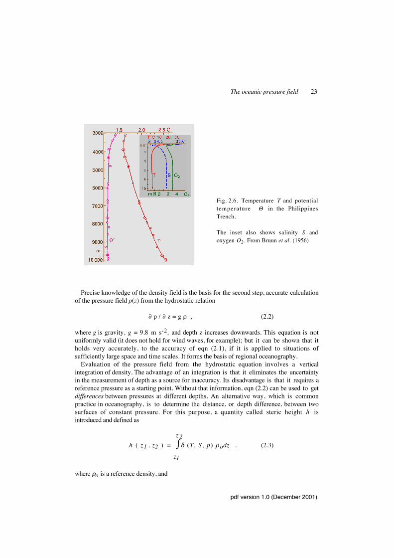
The quality of T and S measurements and of the presently-used equation of state can bechecked by examining data collected in the high pressures found at great depth, where ourmeasurement techniques are given their severest test. Figure 2.6 shows measurements fromthe vicinity of the deepest known place in the ocean. The measured temperature T increaseswith depth over the last six kilometers, while salinity S varies little. In a constant pressureenvironment this would indicate an apparent static instability, i.e. errors in the Equation ofState. However, the same laboratory experiments that gave us the Equation of State allowus to determine very accurately the temperature drop that would occur if a parcel of waterwere brought to the surface without heat exchange. It would cool on decompression,depending on its salinity by 0.03 – 0.12°C per 1 km, and attain its "potential temperature"Θ. Figure 2.6 shows both T and Θ. It is seen that Θ is constant within measurement error.The "potential density" (the density the water would have if it were brought to the surfacewithout changing salinity and potential temperature) is thus constant within measurementerror, too. The available oceanic observations of today show that it is extremely rare to findinversions of potential density, i.e. situations where denser water appears to be lying on topof lighter water. Because in reality such inversions are unstable and overturn very quickly,their absence in observational data implies that eqn (2.1) obtained from laboratorymeasurements is in fact valid in the ocean.



Precise knowledge of the density field is the basis for the second step, accurate calculationof the pressure field p(z) from the hydrostatic relation

∂ p / ∂ z = g ρ , (2.2)

where g is gravity, g = 9.8 m s-2, and depth z increases downwards. This equation is notuniformly valid (it does not hold for wind waves, for example); but it can be shown that itholds very accurately, to the accuracy of eqn (2.1), if it is applied to situations ofsufficiently large space and time scales. It forms the basis of regional oceanography.

Evaluation of the pressure field from the hydrostatic equation involves a verticalintegration of density. The advantage of an integration is that it eliminates the uncertaintyin the measurement of depth as a source for inaccuracy. Its disadvantage is that it requires areference pressure as a starting point. Without that information, eqn (2.2) can be used to getdifferences between pressures at different depths. An alternative way, which is commonpractice in oceanography, is to determine the distance, or depth difference, between twosurfaces of constant pressure. For this purpose, a quantity called steric height h isintroduced and defined as

h ( z1 , z2 ) = ⌡⌠

z1

z 2δ (T, S, p) ρodz , (2.3)

where ρo is a reference density, and

Fig. 2.6. Temperature T and potentialtemperature Θ in the PhilippinesTrench.

The inset also shows salinity S andoxygen O2. From Bruun et al. (1956)



24

δ (T, S, p) = ρ (T, S p)-1 - ρ (0, 35, p)-1 (2.4)

is called the specific volume anomaly; it is the difference in volume between a unit mass ofwater at temperature T and salinity S and a unit mass at the standard salinity S = 35.0 andtemperature T = 0°C. Steric height h has the dimension of height and is expressed inmeters. To sufficient approximation,

δ (T, S, p) = ρo - ρ (T, S, p)

ρ o2 (2.4a)

so that eqn (2.3) can also be written

h (z1 , z2) = ⌡⌠

z1

z 2Δρ (T, S, p) / ρo(p) dz , (2.3a)

where ρo (p) = ρ (0, 35, p) and Δρ (T, S, p) = ρo - ρ (T, S, p). h( z1 , z2) measures theheight by which a column of water between depths z1 and z2 with standard temperatureT = 0°C and salinity S = 35.0 expands if its temperature and salinity are changed to theobserved values. Typically, h is a few tens of centimeters. Because the weight of the wateris not changed during expansion, the pressure difference between top and bottom remainsthe same. It is seen then that h(z1 ,z2) measures variations in the vertical distance betweentwo surfaces of constant pressure.

For oceanographic purposes, the sea surface can always be regarded as an isobaric surface.As any meteorological air pressure map (such as Figure 1.3) tells us, this is only anapproximation. In reality, pressure differences between atmospheric highs and lows are ofthe order of 2 - 3 kPa. However, the ocean reacts to these differences by expanding inregions of low atmospheric pressure and contracting under atmospheric highs. Thesevertical movements are of the order of 0.2 - 0.3 m; like the tides, they have little effect onthe long-term flow field and can be disregarded in our discussion, which is concerned withwater movement induced by the oceanic pressure field.

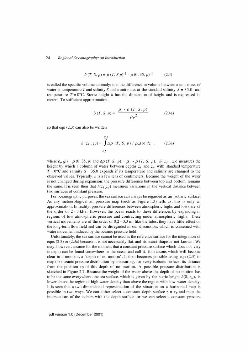
Unfortunately, the sea surface cannot be used as the reference surface for the integration ofeqns (2.3) or (2.3a) because it is not necessarily flat, and its exact shape is not known. Wemay, however, assume for the moment that a constant pressure surface which does not varyin depth can be found somewhere in the ocean and call it, for reasons which will becomeclear in a moment, a "depth of no motion". It then becomes possible using eqn (2.3) tomap the oceanic pressure distribution by measuring, for every isobaric surface, its distancefrom the position z0 of this depth of no motion. A possible pressure distribution issketched in Figure 2.7. Because the weight of the water above the depth of no motion hasto be the same everywhere, the sea surface, which is given by the steric height h(0, zo), islower above the region of high water density than above the region with low water density.It is seen that a two-dimensional representation of the situation on a horizontal map ispossible in two ways. We can either select a constant depth surface z = zr and map theintersections of the isobars with the depth surface, or we can select a constant pressure



surface p1 and draw contours of constant steric height. The first method is well known frommeteorology; daily weather forecasts are based on maps of isobars at sea level (consideredflat for the purpose of meteorology). In oceanography the position of the sea surface isunknown and has to be determined by analysis. Oceanographers therefore map the shape ofthe sea surface by showing contours of equal steric height relative to a depth of no motion,where pressure is assumed to be constant.

It is easy to show - subject to our assumption of a depth of no motion - that at any depthlevel, contours of steric height coincide with contours of constant pressure. The hydrostaticrelation (eqn 2.2) tells us that if pressure is constant at z = zo, the quantity ρo g h ( z, zo)measures the pressure variations along a surface of constant height z. Thus, a contour mapof h is an isobar map scaled by the factor ρo g (see Figure 2.7).

(b) The corresponding pressure map at constant depth z = zr. (c) The corresponding map ofsteric height at constant pressure p = p1.The diagram requires some study, but it is well worth it; understanding these principles is thebasis for the interpretation of many features found in the oceanic circulation.

F ig . 2 .7 . Schemat icillustration of stericheight as a measure ofdistance between isobaricsurfaces, and of the rela-tionship between maps ofisobars a t constantheight and maps of stericheight a t cons tantpressure.(a) Distribution of iso-bars and isopycnals: atany depth level abovez = z o, water at stationA is denser than water atstation B . As the weightof the water abovez = z o is the same, thewater column must belonger at B than at A. Thesteric height of the seasurface relative to z = z ois given by h ( p o, p4),which in oceanographicapplications is oftengiven as h (0, zo), i.e.with reference to depthrather than pressure. Thedifference is negligible.



26

A quantity widely found in oceanographic literature is the dynamic height D. It is definedas

D (p1, p2) = ⌡⌠

p1

p2 δ (T , S , p ) dp (2.5)

and is equal to gh, i.e. the product of gravity and steric height. Maps of dynamic height,also known as dynamic topography maps, are therefore maps of steric height scaled by thefactor g or pressure maps scaled by the factor ρo . We prefer the use of steric height becauseit has the unit of length and therefore can be directly interpreted in terms of, for example,the shape of the sea surface. Other representations do, of course, just as well, as long as weremember that the "dynamic metre" often given as the unit for D is not a length butcorresponds to m2 s-2.

Is it possible to find a flat pressure surface in the ocean, i.e. one where the horizontalpressure gradient vanishes? One consequence of zero horizontal pressure gradient would bethe absence of a current at that depth - hence the name "depth of no motion". Observationssupport the idea that in the deep ocean flow might, indeed, be so slow that the deep pressuremap can be treated as flat. They show that below about 1300 m temperature and salinityare rather uniform, at least within a given basin. This comes out clearly in the maps ofFigure 2.5, which would not show any structure at 2000 m depth outside the SouthernOcean if the relatively coarse contour interval of the 500 m maps were applied here.Furthermore the T and S gradients contribute roughly equal and opposite amounts to thedensity, so that density is remarkably uniform at such depths (even in the Southern Ocean).Within a basin, the density field is so horizontally uniform that steric height at 1500 mrelative to 2000 m, which is shown in Figure 2.8a, displays horizontal variations of onlya centimeter or so, within a given basin - and those variations look so random that they canbe just as much a result of noise in the small data base as a real effect. By contrast, thesteric height map for the sea surface relative to 2000 m (Figure 2.8b) shows differences of0.5 m in a single basin and 1.8 m or so from highest to lowest point in the ocean,because the horizontal gradients of density are much greater (by a factor of several hundred)near the surface than at depths of 1500 - 2000 m.

These facts do not prove that the ocean is moving relatively slowly at depths of 1500 mor 2000 m; all they show is that if flow is slow at the one depth, it is slow at the other.However, in most parts of the ocean similar remarks apply for all pairs of depths (z1, z2)when both lie at or below about 1500 m, so the observations show that if there is anystrong motion at these depths, it must take the form of a nearly vertically uniform floweverywhere below 1500 m. Because of the ocean's rough bottom it seems unlikely thatsuch motions can be very strong or extend over great distances. Unfortunately, directmeasurements of deep ocean currents are much harder to make than measurements oftemperature and salinity; but in most parts of the ocean, such measurements as have beenmade support the idea that flow at these depths is very slow.



Fig. 2.8. Dynamic height (m2 s-2), or steric height multiplied by gravity, for the world ocean.(a) at 1500 m relative to 2000 m, (b) at 0 m relative to 2000 m. Arrows indicate the directionof the implied movement of water, as explained in Chapter 3. (Divide contour values by 10 toobtain approximate steric height in m.) From Levitus (1982).



28

temperature, salinity, density, and the oceanic pressure field

Documents