Ocean Sci., 6, 3–24, 2010www.ocean-sci.net/6/3/2010/© Author(s) 2010. This work is distributed underthe Creative Commons Attribution 3.0 License.

Ocean Science

Density and Absolute Salinity of the Baltic Sea 2006–2009

R. Feistel1, S. Weinreben1, H. Wolf2, S. Seitz2, P. Spitzer2, B. Adel2, G. Nausch1, B. Schneider1, and D. G. Wright3

1Leibniz Institute for Baltic Sea Research, 18119 Warnemunde, Germany2Physikalisch-Technische Bundesanstalt, 38116 Braunschweig, Germany3Bedford Institute of Oceanography, Dartmouth, NS, Canada

Received: 3 August 2009 – Published in Ocean Sci. Discuss.: 19 August 2009Revised: 10 December 2009 – Accepted: 17 December 2009 – Published: 18 January 2010

Abstract. The brackish water of the Baltic Sea is a mixtureof ocean water from the Atlantic/North Sea with fresh wa-ter from various rivers draining a large area of lowlands andmountain ranges. The evaporation-precipitation balance re-sults in an additional but minor excess of fresh water. Therivers carry different loads of salts washed out of the ground,in particular calcium carbonate, which cause a compositionanomaly of the salt dissolved in the Baltic Sea in comparisonto Standard Seawater. Directly measured seawater densityshows a related anomaly when compared to the density com-puted from the equation of state as a function of PracticalSalinity, temperature and pressure.

Samples collected from different regions of the Baltic Seaduring 2006–2009 were analysed for their density anomaly.The results obtained for the river load deviate significantlyfrom similar measurements carried out forty years ago; thereasons for this decadal variability are not yet fully under-stood. An empirical formula is derived which estimates Ab-solute from Practical Salinity of Baltic Sea water, to be usedin conjunction with the new Thermodynamic Equation ofSeawater 2010 (TEOS-10), endorsed by IOC/UNESCO inJune 2009 as the substitute for the 1980 International Equa-tion of State, EOS-80. Our routine measurements of thesamples were accompanied by studies of additional selectedproperties which are reported here: conductivity, density,chloride, bromide and sulphate content, total CO2 and alka-linity.

Correspondence to:R. Feistel(rainer.feistel@io-warnemuende.de)

1 Introduction

In June 2009, the International Thermodynamic Equationof Seawater 2010 (TEOS-10, IOC, 2010) was endorsed bythe IOC1 on its 25th General Assembly in Paris; it will beadopted as a new world-wide standard for oceanography onthe 1 January 2010. TEOS-10 takes Absolute Salinity,SA ,(the mass fraction of sea salt in seawater) as its input variableto represent the concentration of dissolved sea salt in seawa-ter. This choice contrasts with its predecessor, the Interna-tional Equation of State of Seawater 1980 (EOS-80) whichis formulated in terms of Practical Salinity,SP, measuredon the Practical Salinity Scale of 1978 (PSS-78) and repre-senting a measure of the conductivity of a seawater sample.For the first time in the history of oceanographic standardssince 1902, this conceptual transition encourages an explicitconsideration of composition anomalies in the world ocean(McDougall et al., 2009) as well as in estuaries such as theBaltic Sea. In practice, this choice requires the developmentof conversion formulae from Practical Salinity, available forexample from a CTD cast, to Absolute Salinity involvingadditional parameters such as estimates of the compositionanomalies or the geographic position, the depth and, if theanomalies vary significantly on seasonal or climatologicalscales, the time.

For the Baltic Sea, such an algorithm was first publishedby Millero and Kremling (1976), derived from extensivemeasurements (Kremling, 1969, 1970, 1972). Since laterstudies revealed relevant systematic changes of the empiri-cal coefficients (Kremling and Wilhelm, 1997), the first andmain aim of this paper is to propose an updated empiricalformula for the computation of Absolute Salinity of Balticseawater, based on samples taken between 2006 and 2009,for use in conjunction with TEOS-10, as recommended bythe IOC with its recent Resolution XXV-7 (IOC, 2009).

1IOC: Intergovernmental Oceanographic Commission,http://ioc-unesco.org

Published by Copernicus Publications on behalf of the European Geosciences Union.

4 R. Feistel et al.: Density and Absolute Salinity

The composition anomaly of the salt dissolved in theBaltic Sea compared to the composition of Standard Seawa-ter (Millero et al., 2008) is mainly caused by dissolution ofCaCO3 in river water and the subsequent input of Ca2+ andalkalinity/total CO2 into the Baltic Sea by river discharge(Rohde, 1966; Nehring and Rohde, 1967; Kremling, 1969,1970, 1972; Millero and Kremling, 1976). The alkalinity ex-cess controls the pH of the Baltic Sea surface water which atthe present atmospheric CO2 partial pressure ranges between7.8 and 8.2 (Nehring, 1980) and is similar to the pH of oceanwater (Millero, 2007; Marion et al., 2009). Below the perma-nent pycnocline, the pH may decrease to 7.0–7.3 (Fonselius,1967) due to the the accumulation of CO2 by the mineral-ization of organic matter. The second aim of this paper is toestimate the salinity anomaly on the basis of the state of theBaltic Sea CO2 system characterized by the alkalinity andtotal CO2 concentrations. On climatological time scales thealkalinity in the Baltic Sea may increase because the risingatmospheric CO2 may enhance the weathering of CaCO3 inthe catchment area. The increased alkalinity input may affectthe salinity anomaly but also has consequences for the BalticSea acid/base system since it counteracts the pH decrease as-sociated with increasing atmospheric CO2.

An estimate of the CaCO3 excess of the Baltic Sea com-pared to standard seawater is required for chemical compo-sition models of seawater such as FREZCHEM (Feistel andMarion, 2007) which can be used to evaluate the calcium car-bonate supersaturation in relation to atmospheric CO2 levelsand its potential consequences (Marion et al., 2009; Comeauet al., 2009; Veron et al., 2009). Since the density anomalyof the Baltic Sea is varying on climatological time scales, thethird aim of this paper is to provide a more recent anchorpoint for this model in relation to the extended similar in-vestigation made forty years ago by Kremling (1969, 1970,1972) and Millero and Kremling (1976).

The fourth aim of this paper is a conceptual one, related tothe former ones. The different oceanographic salinity scalesthat are in use since 1902 are not metrologically traceableto SI units (Seitz et al., 2008). Both PSS-78 and the recentReference-Composition Salinity Scale (Millero et al., 2008)are defined in terms of relative conductivity measurementswith artefacts such as IAPSO2 Standard Seawater (SSW) ora potassium chloride solution used as a reference. Relianceon such artificial references introduces the risk of unnoticedor falsly indicated property changes over time or between dif-ferent samples. It would therefore be preferable to establishtraceability to the highly reliable and independently realis-able standards of the International System of Units (Jones,2009). The SCOR3/IAPSO Working Group 127 (WG127)on the Thermodynamics and Equation of State of Seawater

2IAPSO: International Association for the Physical Sciences ofthe Ocean,http://iapso.sweweb.net

3SCOR: Scientific Committee on Oceanic Research,http://www.scor-int.org

is currently developing a new concept for the measurementof Absolute Salinity based on SI-traceable density determi-nations (Wolf, 2008). The Baltic Sea with its strong densityanomaly and pronounced trends in its properties is a promi-nent example of the need for the development of this ap-proach and a useful testing ground for the new but yet imma-ture calibration technology. For this reason, we have carriedout comparison measurements of conductivity and densityin an SI-traceable way and we report the results in this pa-per. The presentation of results is accompanied by selectedchemical composition data.

The true Absolute Salinity is defined in terms of the massfraction of dissolved material in seawater (Millero et al.,2008). As discussed by Millero et al., the precise defini-tion requires the determination of equilibrium conditions atspecified temperature and pressure and even with these addi-tional qualifiers some ambiguity remains. In practice, mea-suring the mass fraction of dissolved material in seawateris even more difficult than defining it and approximate ap-proaches must be used. It is the “Millero Rule” that saysthat the density of an aqueous solution is in good approxima-tion a function of the Absolute Salinity, independent of theparticular composition of the given mass of dissolved matter(Millero, 1974; Millero et al., 1978, 2008, 2009). Under thisapproximation, Baltic seawater and Standard Seawater havethe same Absolute Salinity if they have the same density atgiven temperature and pressure. Thus, we can measure thedensity of Baltic seawater, and use the TEOS-10 equation ofstate to compute the Absolute Salinity of Standard Seawaterwith this density. We then use Millero’s Rule and take this“density salinity” as an estimate for the mass of salt dissolvedin the Baltic Sea sample. We note however that the true Ab-solute Salinity is defined as the mass ratio of dissolved ma-terial and that Millero’s Rule provides an approximation tothis quantity. Unfortunately, for seawater that is not of Ref-erence Composition there is currently no method available toprecisely measure the Absolute Salinity, but Millero’s Ruleprovides an approximation that allows the density to be re-covered to the measurement accuracy (due to the use of the“density salinity” to estimate Absolute Salinity) as well asa useful approximation for other thermodynamic quantitiesthat can be determined from the TEOS-10 Gibbs function(IAPWS, 2008; IOC, 2010; Feistel et al., 2009; Wright et al.,2009).

2 Salinity of standard and baltic seawater based onprevious measurements

Since the introduction of the Practical Salinity Scale, theelectrolytic conductivityC of a seawater sample is practi-cally measured by salinometers or conductivity sensors, cal-ibrated with respect to a certified IAPSO Standard Seawa-ter reference. The measured conductivity ratio is convertedto conductivity usingC = 4.2914 S m−1 at SP = 35, t=15◦C

Ocean Sci., 6, 3–24, 2010 www.ocean-sci.net/6/3/2010/

R. Feistel et al.: Density and Absolute Salinity 5

andP = 101325 Pa (Culkin and Smith, 1980; SeaBird, 1989)and fromC, the temperatureT and the pressureP , PracticalSalinitySP is computed from the function (Perkin and Lewis,1980)

SP= s (C,T ,P ). (1)

Over the range of concentrations where Practical Salinity isdefined, it can be converted to Reference Salinity,SR, bythe factoruPS= (35.16504 g kg−1)/35 (Millero et al., 2008,Feistel, 2008):

SR = SP·uPS. (2)

For Standard Seawater,SR is the most accurate estimatecurrently available for the Absolute Salinity. GivenSR,the corresponding density estimate can be determined fromthe Gibbs functiong(SR,T ,P ) of seawater (Feistel, 2008;IAPWS, 2008; IOC, 2010):

ρ =1

gP (SR,T ,P )(3)

Here, the subscriptP denotes the partial derivative with re-spect to the pressure, andT andP are the temperature andpressure at which the density is required, e.g. at laboratoryconditions.T andP will be omitted from the equations be-low for simplicity. In the case of Standard Seawater, (Eq. 3)provides our best estimate of the true density,ρSSW. In thecase of Baltic seawater, (Eq. 3) yields an apparent densitythat is subject to significant error. The anomaly of the trueBaltic seawater density relative to this rather uncertain esti-mate can be determined by measuring the true density,ρBSW,with a vibration densitometer (Kremling, 1971; Millero andKremling, 1976). The Absolute Salinity,SBSW

A = SR+δSA ,of Baltic seawater can then be estimated by the “densitysalinity”, i.e., by computing the Absolute Salinity of Stan-dard Seawater giving the measured density of Baltic seawa-ter, from the formula (Millero et al., 2008),

ρBSW=

1

gP (SR+δSA)≈

1+β ·δSA

gP (SR), (4)

i.e.,δSA =(ρBSWgP −1

)/β. Here,β = −gSP /gP is the ha-

line contraction coefficient.In Fig. 1, the anomalySBSW

A − SR is shown as a func-tion of SR for 153 samples collected 40 years ago by Krem-ling (1969, 1970, 1972), computed by means of (Eqs. 2–4)from the published values of measured Practical Salinity,SP,and the measured density,

The correlation relating “density salinity” to PracticalSalinity is easily obtained since both Practical Salinity anddensity are easily measured on a regular basis. Based onKremling’s data, the regression line is

δSA = SA −SR = 0.00428·(SSO−SR)

= 150mgkg−1·

(1−

SR

SSO

). (5)

0 5 10 15 20 25 30 350

20

40

60

80

100

120

140

160

Salin

ity A

nom

aly

( S

A -

S R) /

(m

g/kg

)

Reference Salinity SR / (g/kg)

Baltic Density Anomaly 1966-69

x

x

x

x

x

x

x

x

xx

x

x

x

xx

xx

x

x

x

xx

x

xxx

x

x

xx

x

x

x

xxx

x

x

xx

xx

x

x

xxx

x

xx

xx

x

x

x

x

x

x

x

x

xx

x

x

x

xx

x

x

xx

x

x

xxx

x

xxx

x

x

xx

xxx

x

x

xx

xx

xx

x

xx

xxx

x

x

x

x

x

x

x

xxx

x

x

xxx

x

xx

x

x

x

x

x

x

x

xx

xxx

x

x

x

x

x

x

xx

xx

xx

x

x

x

x

xxx

x

x

x

x

x

x

xx

xx

x

xx

xx

x

x

x

x

x

x

x

x

x

xx

x

x

xxx

x

xx

x

xx

x

x

xx

x

xx

xx

x

x

x

x

xx

x

x

xx

xxx

x

x

x

x

x

x

x

x

x

x

x

x

x

x

x

x

xxxxx

x

xx

x

x

xx

x

x

xxx x

x

x

x

x

x

x

xx

x

x

x

x

x

x

x

xxx

x

xxxx

xx

x

x

x

x

x

x

x

x

xx

xx

x

xxx

x

xxx

x

x

x

x

x

xxx

xxx

xx

x

x

xxx

xx

x

x

x

xxxx

xxx

x

x

x

x

x

x

x

x

x

xx

x

x

x

xx

x

x

xx

x

x

xxx

x

x

x

xxxxxxxx

xxx

x

x

x

xx

x

x

xxx

x

x

x

x

xx

x

xx

xxx

x

x

x

xxx

xx

x

xx

x

xxxx

x

x

xxx

x

x

x

x

xx

x

xxx

x

x

x

xx

x

x

x

x

x

x

x

xxx

x

xxxx

x

x

xx

xx

xx

x

x

xxxx

xx

x

xx

x

x

xxx

xxx

x

x

x

xxx

x

x

x

xx

x

xx

x

x

xx

x

x

x

xxx

x

x

x

x

xx

xx

xx

x

xxxxx

xxx

xx

xx

xx

x

x

xx

x

x

xxxx

x

x

xxx

x

x

x

xx

x

xxxxx

x

x

x

xx

x

xx

x

x

xx

x

x

x

xx

x

xx

x

x

x

xx

x

xxx

x

x

xxx

xxxxx

xxxx

x x

x

xxx

x

xxxx

xxxxxx

xxx

xx

xxx

xxxx

x

x

x

xx

x

x

x

xx

xxxxx

xx

xxx

xx

xxx

x

xxx

x

x

x

xxx

x

x

x

x

x

x

x

x

x

xx

xxx

x

x

x

x

x

xx

xx

x

x

x

xxx

x

xx

x

xx

x

xxx

xx

xx

xxx

1966 - 1969

Fig. 1: Salinity anomaly RAA SSS −=δ computed by means of eqs. (2) - (4) from Practical Salinity and density data measured by Kremling (1969, 1970, 1972) and Millero and Kremling (1976) in the period 1966-1969. The sample near SR = 4 g/kg with exceptionally low anomaly was excluded from the fit (5); it was collected in the Vistula Estuary.

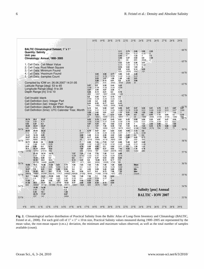
The strong scatter visible in Fig. 1 at very low salinities is due to the inhomogeneous water properties caused by the very different loads of the many discharging rivers. The sampling is patchy, but adequate for the present purpose. The calcium carbonate that is primarily responsible for the Absolute Salinity anomalies is mainly carried by rivers draining the European lowlands, while the Scandinavian rivers flow over solid rocks and are subsaturated with respect to lime (Kwiecinski, 1965). Spatial distributions of the river water age (Meier, 2007) indicate weak lateral mixing of the properties between the various rivers which contributes to the spatial inhomogeneity of the Baltic surface water. In lowest order, the structure of the mean surface current is evident from the climatological horizontal salinity gradient, Fig. 2 (Feistel et al., 2008). The Baltic has a mean basin-scale circulation that is predominantly estuarine (vertical) rather than horizontal (see the schematic flow diagram in Fig. 10.1 of Matthäus et al., 2008, available at http://www2008.io-warnemuende.de/baltic2008/figures/figures_of_chapter_10.pdf ). Precipitation and fresh riverine water is added to the surface, and over time the surface water is enriched with salt from below by entrainment. The diffusive transport of saline water into the Baltic from the North Sea is negligible and strongly dominated by the permanent upward salt transport through the halocline at about 60 m depth, which has been roughly estimated as 30 kg m–2 yr–1, consistently from different approaches (Feistel et al., 2008; Reissmann et al., 2009). Consequently, the climatological surface salinity increases following the mean surface flow from the north-east to the south-west. Brackish surface water is present in the outflow

Fig. 1. Salinity anomalyδSA = SA −SR computed by means of(Eqs. 2–4) from Practical Salinity and density data measured byKremling (1969, 1970, 1972) and Millero and Kremling (1976) inthe period 1966–1969. The sample nearSR = 4 g/kg with excep-tionally low anomaly was excluded from the fit (Eq. 5); it was col-lected in the Vistula Estuary.

The fit was constrained to pass through (SR = SSO, δSA =

0) because the Atlantic water part of the brackish mix-ture is free of the Baltic anomaly (Millero and Kremling,1976). Here, the standard-ocean salinity isSSO= 35uPS=

35.16504gkg−1 (Millero et al., 2008).The strong scatter visible in Fig. 1 at very low salinities

is due to the inhomogeneous water properties caused by thevery different loads of the many discharging rivers. The sam-pling is patchy, but adequate for the present purpose. Thecalcium carbonate that is primarily responsible for the Abso-lute Salinity anomalies is mainly carried by rivers drainingthe European lowlands, while the Scandinavian rivers flowover solid rocks and are subsaturated with respect to lime(Kwiecinski, 1965). Spatial distributions of the river waterage (Meier, 2007) indicate weak lateral mixing of the prop-erties between the various rivers which contributes to the spa-tial inhomogeneity of the Baltic surface water. In lowest or-der, the structure of the mean surface current is evident fromthe climatological horizontal salinity gradient, Fig. 2 (Feistelet al., 2008). The Baltic has a mean basin-scale circulationthat is predominantly estuarine (vertical) rather than horizon-tal (see the schematic flow diagram in Fig. 10.1 of Matthauset al., 2008, available athttp://www2008.io-warnemuende.de/baltic2008/figures/figuresof chapter10.pdf). Precipita-tion and fresh riverine water is added to the surface, andover time the surface water is enriched with salt from be-low by entrainment. The diffusive transport of saline wa-ter into the Baltic from the North Sea is negligible andstrongly dominated by the permanent upward salt trans-port through the halocline at about 60 m depth, which hasbeen roughly estimated as 30 kg m−2 yr−1, consistently from

www.ocean-sci.net/6/3/2010/ Ocean Sci., 6, 3–24, 2010

6 R. Feistel et al.: Density and Absolute Salinity

branch of the Baltic “conveyor belt” that drives the Baltic Current along the Norwegian coast; saltier water from the North Sea is flowing in at the bottom. In the shallow Belt Sea, strong mixing occurs between the inflowing and outflowing layers that implies a recirculation of significant freshwater fractions as a part of the salty bottom water. In addition to the salt, entrainment from below the pycnocline adds aged, mixed and possibly chemically transformed riverine solutes to the surface layer (Reissmann et al., 2009). In the deep water of the estuarine Baltic Sea environment, the dissolved species may be subjected to either reducing or oxidizing conditions that are sustained for extended periods of time (Nausch et al., 2008). The time scales associated with these processes are of the order of decades (Stigebrandt and Wulff, 1989; Meier et al., 2006; Feistel et al., 2008).

53°N

54°N

55°N

56°N

57°N

58°N

59°N

53°N

54°N

55°N

56°N

57°N

58°N

59°N

60°N

61°N

62°N

63°N

64°N

65°N

66°N

18°E 19°E 20°E 21°E 22°E 23°E 24°E 25°E 26°E 27°E 28°E 29°E

9°E 10°E 11°E 12°E 13°E 14°E 15°E 16°E 17°E 18°E 19°E 20°E 21°E 22°E 23°E 24°E 25°E 26°E 27°E 28°E 29°E

BALTIC Climatological Dataset, 1° x 1°Quantity: SalinityUnit: psuClimatology: Annual, 1900- 2005

1. Cell Data: Cell Mean Value2. Cell Data: Root Mean Square3. Cell Data: Minimum Found4. Cell Data: Maximum Found5. Cell Data: Samples Count

Compiled by IOW on: 26.06.2007 14:31:05Latitude Range [deg]: 53 to 65Longitude Range [deg]: 9 to 29Depth Range [m]: 0 to 10

Cell Invalid: blankCell Definition (lon): Integer PartCell Definition (lat): Integer PartCell Definition (depth): All Within RangeCell Definition (time): UTC Calendar Year, Month

20.743.294.0232.6244028.653.4212.4134.57206132.711.1823.935.414152

18.982.6310.3731.62860816.12.111.8421.38504

25.23.875.8434.04235629.443.0310.1635.13889528.343.669.6635.141478123.183.3210.4433.352572618.43.157.433.357499115.892.8529.53060214.382.645.4520.72237

23.074.716.334.2712926.233.456.0534.518915243.656.434.612151419.743.298.8833.91444915.483.466.3134.12039412.872.735.0826.813974212.381.5510.117.57141

20.593.059.7433.896218.133.55.234.42639511.943.554.8135.75831510.491.895.0825141066

8.010.535.9821.52174178.020.551.8717.1270156

7.740.385.3911.05248627.670.522.6510.62289106.350.81.588.672454

7.570.296.69.146007.560.33.49.5368387.630.333.389.4710651

60.673.087.292270.384.787.853557.290.345.18.6412717.550.33.19.36215527.480.35.468.981824

5.070.483.076.094535.40.333.596.047905.160.363.595.76276.020.055.976.136.790.45.488.1720166.990.325.698.9450537.190.334.778.59907.530.314.659.1798497.360.266.628.09423

4.940.572.035.882735.20.382.946.1412875.550.263.26.3514835.60.313.626.4918375.790.564.247.071606.670.385.148.0655697.060.335.928.667317.320.475.2710.8583507.450.33.299.4113467.10.591.048.293570

4.580.761.076.156165.390.334.076.2118575.710.223.396.1718255.580.313.916.543695.970.374.87.4630506.90.344.387.8941167.230.323.38.37122077.380.295.538.14103357.480.283.498.7331587.350.3718.197087

4.770.591.086.9134435.440.333.366.323985.750.223.016.4133595.970.293.276.535196.450.484.829.3912376.830.384.428.0238207.270.325.848.62206757.170.293.928.1727937.280.295.897.9814576.6406.646.642

3.110.482.433.4663.220.252.133.96333.960.421.965.530945.250.3616.1611205.60.31.266.4336406.060.261.156.9458816.610.393.127.8156726.930.375.837.632086.980.423.717.658996.960.146.657.1656.620.322.557.32270

2.740.6113.37693.340.222.644.5320293.420.241.025.142039

6.070.195.316.44776.320.462.367.5460675.690.115.525.86275.480.344.66.93405

3.060.371.333.928553.360.191.045.1433673.380.212.813.6641

2.370.261.064.4245.990.6518.1661845.320.463.46.852305.270.311.397.361382

2.950.3513.925283.470.2234.03131

5.450.511.536.513005.690.511.517.2374654.80.582.45.733505.020.441.215.76680

2.3502.32.392

5.310.491.066.9329465.350.542.988.443174

4.750.521.317.1521944.970.632.886.78704

4.110.5115.6451934.470.51.45.88478

2.870.671.025.712824.040.81.655.8971

2.270.6915.19688

Meanr.m.s.MinMaxCount

Salinity [psu] Annual BALTIC - IOW 2007

Fig. 2: Climatological surface distribution of Practical Salinity from the Baltic Atlas of Long-Term Inventory and Climatology (BALTIC, Feistel et al., 2008). For each grid cell of 1° x 1° x 10 m size, Practical Salinity values measured during 1900 – 2005 are represented by the mean value, the root-mean square (r.m.s.) deviation, the minimum

Fig. 2. Climatological surface distribution of Practical Salinity from the Baltic Atlas of Long-Term Inventory and Climatology (BALTIC,Feistel et al., 2008). For each grid cell of 1◦

×1◦×10 m size, Practical Salinity values measured during 1900–2005 are represented by the

mean value, the root-mean square (r.m.s.) deviation, the minimum and maximum values observed, as well as the total number of samplesavailable (count).

Ocean Sci., 6, 3–24, 2010 www.ocean-sci.net/6/3/2010/

R. Feistel et al.: Density and Absolute Salinity 7

different approaches (Feistel et al., 2008; Reissmann et al.,2009). Consequently, the climatological surface salinity in-creases following the mean surface flow from the north-eastto the south-west. Brackish surface water is present in theoutflow branch of the Baltic “conveyor belt” that drives theBaltic Current along the Norwegian coast; saltier water fromthe North Sea is flowing in at the bottom. In the shallowBelt Sea, strong mixing occurs between the inflowing andoutflowing layers that implies a recirculation of significantfreshwater fractions as a part of the salty bottom water.

In addition to the salt, entrainment from below the pycno-cline adds aged, mixed and possibly chemically transformedriverine solutes to the surface layer (Reissmann et al., 2009).In the deep water of the estuarine Baltic Sea environment, thedissolved species may be subjected to either reducing or ox-idizing conditions that are sustained for extended periods oftime (Nausch et al., 2008). The time scales associated withthese processes are of the order of decades (Stigebrandt andWulff, 1989; Meier et al., 2006; Feistel et al., 2008).

In the special case in which the stoichiometric deviationfrom the Reference Composition is caused by an excess ofnon-conducting solutes with low concentrations, the value ofSR represents the mass fraction of sea salt with ReferenceComposition in the sample, andδSA represents the anoma-lous mass fraction of non-conducting species, at least to apractically reasonable accuracy. This can safely be assumedfor the silicate anomaly in the North Pacific (McDougallet al., 2009), but it is not generally the case in the BalticSea since the additional CaCO3 dissociates and increasesthe conductivity by a non-zero amount, evidently less thanwhat would result from adding the same mass of sea saltthat has Reference Composition. Similarly, the algorithmsused to estimate Practical Salinity at temperatures and pres-sures different from 15◦C and 101 325 Pa are not valid in thepresence of the composition anomalies and (Eq. 1) resultsin inconsistent estimates, which can result in the appearancethat the salinity is not conservative when subjected to tem-perature or pressure changes. Consequently, the correlationshown in Fig. 1 may look different depending on the particu-lar T or P at which the measurements were carried out in thelab. However, a study dedicated to this problem (Feistel andWeinreben, 2008) came to the conclusion that these apparentnon-conservation effects for Baltic seawater do not exceedthe measurement uncertainty over a reasonable temperatureinterval at atmospheric pressure. Consequently, the param-eterisation of the Absolute Salinity of Baltic Sea water as afunction of Reference Salinity is stable with respect to tem-perature variations at atmospheric pressure and is thus justi-fied for application in the context of TEOS-10 (IOC, 2010).

The above approach to estimating Absolute Salinity re-lies on an empirical relation between Absolute and PracticalSalinity in the Baltic Sea. It does not permit the separateestimation of the contributions from riverine input into theBaltic Sea and from the sea salt flowing in from the Atlantic.This separation is possible using measurements of the chlo-

rinity, Cl, rather than conductivity since no relevant amountsof chlorine, bromine or iodine are discharged from the trib-utaries. Chlorinity can thus be used to estimate the Abso-lute Salinity contribution associated with input from the At-lantic and subtracting this value from the density salinity willprovide an estimate of the contribution associated with localinputs. Millero and Kremling (1976) performed their corre-lation analysis based on chlorinity data. Two drawbacks ofthis method are that chlorinity is not a concentration measureto be used with TEOS-10, and silver titrations are not carriedout regularly on modern research or monitoring cruises in theBaltic. Nevertheless, the approach can be used to separatethe salt inputs from the Atlantic and from local runoff andto provide a comparison with the conditions found earlier byKnudsen (1901) and Sørensen (Forch et al., 1902).

For Standard Seawater, the Reference SalinitySR can becomputed from the chlorinity by multiplying by the factoruCl = 1.80655·uPS (Millero et al., 2008; Feistel, 2008). ForBaltic Sea water the result will differ fromSR, and is there-fore referred to here as “chlorinity salinity”,SCl :

SCl = Cl ·uCl = 180655·Cl ·uPS (6)

Using the chlorinity,Cl, and the density,ρBSW, data mea-sured by Kremling (1969, 1970, 1972) and Millero andKremling (1976) together with (Eq. 4) in the form,

ρBSW=

1

gP

(SCl +δSRI

) ≈1+β ·δSRI

gP (SCl), (7)

the regression line for the river input,δSRI, Fig. 3, is deter-mined as

δSRI= SA −SCl = 000492·(SSO−SCl)

= 173mgkg−1·

(1−

SCl

SSO

). (8)

The difference between (Eqs. 5 and 8) is caused by the factthat the riverine input includes calcium carbonate and othersolutes which alter the impact on the electrical conductivitycompared to the effect of diluting with pure water whereasthe riverine input includes no corresponding input of halides.Because of this latter fact, the intercept atSCl = 0 corre-sponds to no contribution from North Atlantic water and pro-vides a direct estimate of the contribution to Absolute Salin-ity due to the salt content of the local riverine inputs.

Millero and Kremling (1976) did an analogous fit to theirdata set with 153 samples but found an intercept at zero chlo-rinity of only S0

A = 124mgkg−1. The reason for this differ-ence is probably the older equation of state used at that time(F. J. Millero, personal communication, 2009).

It is also possible to estimate the relation correspondingto (Eq. 8) based on data from the early 20th century. TheKnudsen (1901) EquationSK = 0.03gkg−1

+1.805Cl, wascalculated from Sørensen’s analysis of 9 surface water sam-ples, including 6 from the Baltic Sea, in particular, one fromthe Gulf of Finland, one from Gulf of Bothnia, two from the

www.ocean-sci.net/6/3/2010/ Ocean Sci., 6, 3–24, 2010

8 R. Feistel et al.: Density and Absolute Salinity

( ) ( )Cl

RI

RICl

BSW 11Sg

SSSg PP

δβδ

ρ ×+≈+

= , (7)

the regression line for the river input, RISδ , Fig. 3, is determined as

( ) ���

����

�−×=−×=−= −

SO

Cl1ClSOClA

RI 1kgmg17300492.0SS

SSSSSδ . (8)

The difference between (5) and (8) is caused by the fact that the riverine input includes calcium carbonate and other solutes which alter the impact on the electrical conductivity compared to the effect of diluting with pure water whereas the riverine input includes no corresponding input of halides. Because of this latter fact, the intercept at SCl = 0 corresponds to no contribution from North Atlantic water and provides a direct estimate of the contribution to Absolute Salinity due to the salt content of the local riverine inputs. Millero and Kremling (1976) did an analogous fit to their data set with 153 samples but found an intercept at zero chlorinity of only 10

A kgmg124 −=S . The reason for this difference is probably the older equation of state used at that time (F.J. Millero, pers. comm.).

0 5 10 15 20 25 30 350

20

40

60

80

100

120

140

160

180

Salin

ity A

nom

aly

( S A

- S C

l) /

(mg/

kg)

Chlorinity Salinity SCl / (g/kg)

Baltic Density Anomaly 1966-69

x

x

x

x

x

x

x

x

xxx

x

x

xx

xx

x

x

x

xx

x

xxx

x

x

xx

x

x

x

xxx

x

x

xx

xx

x

x

xxx

x

xxxx

x

x

x

x

x

x

x

x

xx

x

x

x

xx

x

x

xx

x

x

xxx

x

xxx

x

x

xxxx

x

x

x

xx

xx

xxx

xx

xxx

x

xx

x

x

x

x

xxx

xx

xxx

x

xx

x

x

x

x

x

xx

xx

xxx

x

x

x

x

x

x

xx

xx

xx

x

x

xx

xxx

x

xx

x

x

x

xx

xx

x

xx

xx

x

x

x

x

x

x

x

x

x

xx

x

x

xxx x

x

xxx

x

xx

x

xx

x

x

xx

xxx

xx

x

x

xx

xx

x

x

xx

xxx

x

x

x

x

x

x

x

x

x

x

x

x

x

x

x

x

xxxxx

x

xx

x

x

xx

x

x

xxx

x

x

x

x

x

xx

xx

x

x

x

x

x

x

x

xxx

x

xxxxxx

xx

x

x

x

xxx

x

xxx

x

xxx

x

xxx

x

x

x

xx

xxx xxx

xx

x

x

xxx

xx

xxx

x

xxx

xxx

x

x

x

xx

x

x

x

x

xx

x

x

x

xx

xx

xx

x

x

xxx

x

x

x

xxxxxxxxxxx

x

x

x

xx

x

x

xxx

x

x

x

x

xxx

xx

xxx

x

xxxxx

xx

x

xx

x

xxxx

x

x

xxxx

x

xx

xx

x

xxx

x

x

xxx

x

x

x

x

x

x

x

xxx

x

xxxx

x

x

xx

xx

xx

x

xxxxx

xx

x

xx

x

x

xxx

xxx

x

x

x

xxx

x x

x

xx

x

x xx

x

xxx

x

x

x

xxx

x

x

x

x

xx

xx

xxx

xxxxx

xxxxx

xx

xx

xx

xx

x

x

xxxx

x

x

xxxx

x

x

xx

xxxxxx

x

x

x

xx

x

xx

x

x

xx

x

x

x

xx

x

xx

x

x

x

xx

x

xxx

x

x

xxx x

xxxxxx

xxx

x

x

xxx

x

xxxx x

xxxxx

xxx

xx

xxx

xxxx

x

x

x

xx

x

x

x

xx

xxxxx

xx

xxx

xx

xxx

x

xxx

x

x

x

xxx

xx

x

x

x x

x

x

x

x

x

xxx

x

x

x

x

xxx

xx

xx

xxxx

x

xx

x

xx

x

xxx

xx

xx

xxx

SS

S

S

S

S

1966 - 1969

Knudsen 1901

Fig. 3: Salinity anomaly associated with local runoff ClACl SSS −=δ computed by means of eqs. (4) - (6) from chlorinity and density data, symbol “x”, measured by Kremling (1969, 1970, 1972) and Millero and Kremling (1976) in the period 1966-1969. The sample with exceptionally low anomaly collected in the Vistula Estuary was excluded

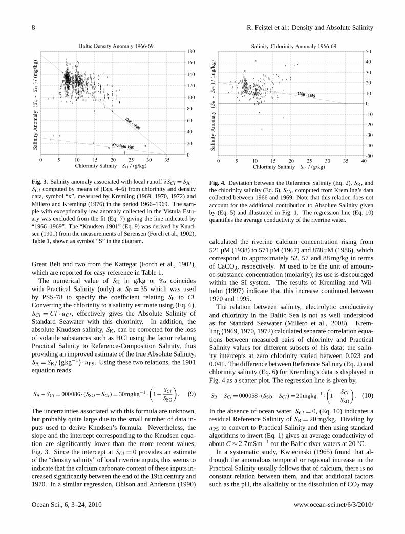
Fig. 3. Salinity anomaly associated with local runoffδSCl = SA −

SCl computed by means of (Eqs. 4–6) from chlorinity and densitydata, symbol “x”, measured by Kremling (1969, 1970, 1972) andMillero and Kremling (1976) in the period 1966–1969. The sam-ple with exceptionally low anomaly collected in the Vistula Estu-ary was excluded from the fit (Eq. 7) giving the line indicated by“1966–1969”. The “Knudsen 1901” (Eq. 9) was derived by Knud-sen (1901) from the measurements of Sørensen (Forch et al., 1902),Table 1, shown as symbol “S” in the diagram.

Great Belt and two from the Kattegat (Forch et al., 1902),which are reported for easy reference in Table 1.

The numerical value ofSK in g/kg or ‰ coincideswith Practical Salinity (only) atSP = 35 which was usedby PSS-78 to specify the coefficient relatingSP to Cl.Converting the chlorinity to a salinity estimate using (Eq. 6),SCl = Cl · uCl , effectively gives the Absolute Salinity ofStandard Seawater with this chlorinity. In addition, theabsolute Knudsen salinity,SK , can be corrected for the lossof volatile substances such as HCl using the factor relatingPractical Salinity to Reference-Composition Salinity, thusproviding an improved estimate of the true Absolute Salinity,SA = SK/

(gkg−1)

·uPS. Using these two relations, the 1901equation reads

SA −SCl = 000086·(SSO−SCl) = 30mgkg−1·

(1−

SCl

SSO

). (9)

The uncertainties associated with this formula are unknown,but probably quite large due to the small number of data in-puts used to derive Knudsen’s formula. Nevertheless, theslope and the intercept corresponding to the Knudsen equa-tion are significantly lower than the more recent values,Fig. 3. Since the intercept atSCl = 0 provides an estimateof the “density salinity” of local riverine inputs, this seems toindicate that the calcium carbonate content of these inputs in-creased significantly between the end of the 19th century and1970. In a similar regression, Ohlson and Anderson (1990)

0 5 10 15 20 25 30 35 40-50

-40

-30

-20

-10

0

10

20

30

40

50

Salin

ity A

nom

aly

( S R

- S C

l) /

(mg/

kg)

Chlorinity Salinity SCl / (g/kg)

Salinity-Chlorinity Anomaly 1966-69

x

x

x

x

xx

x

xx

xx

x

xx x

xx

x

xx

x x

x

x

x x

x xx

x

x xx

x

x

x

x

x

x

x

x

xx

xx

x

xx

x

x

x

xx

x

x

x

x

x

x

x

xx

x

x

x

xx

xx

x

xx

x

xx

x

x

x

xxxxx

xx

x

xx

x

x x

x

x

xx

x

xx

x x x xx

x

x xx

x

x

x

xxx x

xx x

x

xx

xxxx

x

x

x

xx

xx x x

x

x x xxx

xx

x

x

x

x

x

x

x

xx

xx

x

xx

xx

xx

xx x

x

x

x

x

x x

x

xx

x

xx

x x

x

x

x

xx

x

x

x

x

x

x

x

xx

x

x

xx

x

x

x

x

x

xx

x

xx

x

x

x

x

x

x

xx

x

x

xx

xx

x

xx

xx

x

1966 - 1969

Fig. 4: Deviation between the Reference Salinity (2), SR, and the chlorinity salinity (6), SCl, computed from Kremling’s data collected between 1966 and 1969. Note that this relation does not account for the additional contribution to Absolute Salinity given by (5) and illustrated in Fig. 1. The regression line (10) quantifies the average conductivity of the riverine water.

In a systematic study, Kwiecinski (1965) found that although the anomalous temporal or regional increase in the Practical Salinity usually follows that of calcium, there is no constant relation between them, and that additional factors such as the pH, the alkalinity or the dissolution of CO2 may be important. Numerical composition models (Anderko and Lencka, 1997; Feistel and Marion, 2007; Pawlowicz, 2008, 2009) may provide more detailed insight in the future. The composition of the Baltic Sea salt measured by different authors was summarized by Nehring (1980) as given in Table 1 in comparison to the Reference Composition (Millero et al., 2008). Table 1: Ratios rX = w(X)/Cl of mass fractions w(X) to chlorinity Cl of the main sea salt constituents X compiled by Millero et al. (2008) for Standard Seawater and by Nehring (1980) for Baltic seawater from different sources. Molar masses AX are those compiled by Millero et al. (2008). The oceanic value of rCl = [1/(0.3285234 AAg) – rBr

/ ABr] × ACl is inferred from the definition of chlorinity, using the molar mass AAg = 107.8682(2) g/mol of silver. The Baltic rCl is calculated from the same formula using Kremling’s value for rBr. The numbers in brackets are the standard uncertainties of the corresponding digit(s) in front of the opening bracket.

Fig. 4. Deviation between the Reference Salinity (Eq. 2),SR, andthe chlorinity salinity (Eq. 6),SCl , computed from Kremling’s datacollected between 1966 and 1969. Note that this relation does notaccount for the additional contribution to Absolute Salinity givenby (Eq. 5) and illustrated in Fig. 1. The regression line (Eq. 10)quantifies the average conductivity of the riverine water.

calculated the riverine calcium concentration rising from521 µM (1938) to 571 µM (1967) and 878 µM (1986), whichcorrespond to approximately 52, 57 and 88 mg/kg in termsof CaCO3, respectively. M used to be the unit of amount-of-substance-concentration (molarity); its use is discouragedwithin the SI system. The results of Kremling and Wil-helm (1997) indicate that this increase continued between1970 and 1995.

The relation between salinity, electrolytic conductivityand chlorinity in the Baltic Sea is not as well understoodas for Standard Seawater (Millero et al., 2008). Krem-ling (1969, 1970, 1972) calculated separate correlation equa-tions between measured pairs of chlorinity and PracticalSalinity values for different subsets of his data; the salin-ity intercepts at zero chlorinity varied between 0.023 and0.041. The difference between Reference Salinity (Eq. 2) andchlorinity salinity (Eq. 6) for Kremling’s data is displayed inFig. 4 as a scatter plot. The regression line is given by,

SR−SCl = 000058·(SSO−SCl) = 20mgkg−1·

(1−

SCl

SSO

). (10)

In the absence of ocean water,SCl = 0, (Eq. 10) indicates aresidual Reference Salinity ofSR = 20 mg/kg. Dividing byuPS to convert to Practical Salinity and then using standardalgorithms to invert (Eq. 1) gives an average conductivity ofaboutC ≈ 2.7mSm−1 for the Baltic river waters at 20◦C.

In a systematic study, Kwiecinski (1965) found that al-though the anomalous temporal or regional increase in thePractical Salinity usually follows that of calcium, there is noconstant relation between them, and that additional factorssuch as the pH, the alkalinity or the dissolution of CO2 may

Ocean Sci., 6, 3–24, 2010 www.ocean-sci.net/6/3/2010/

R. Feistel et al.: Density and Absolute Salinity 9

Table 1. Samples collected from the Baltic Sea in 1900 and analysed by Sørensen (Forch et al., 1902). It may be the extreme effort of salinitydetermination by drying at 150–480◦C over 120 h that prevented Sørensen from the analysis of all available samples. Additional samplestaken from outside the Baltic Sea are omitted from this table.

Sample Cl ‰ SK ‰ N. Lat. E. Lon. Depth m Date, Time Sea

#32 1.4736 2.688 60◦07′ 28◦33.5′ 0 19 July 1900, 20:50 G. Finland#33 2.9274 5.321 62◦07′ 20◦02′ 0 24 July 1900, 15:00 G. Bothnia#29 4.6075 54◦39.5′ 12◦17.3′ 0 7 May 1900, 08:00 Belt Sea#30 8.0888 14.634 55◦42.2′ 10◦43.7′ 0 8 May 1900, 14:10 Gr. Belt#9 10.4102 18.818 55◦52′ 10◦52′ 0 23 April 1900, 18:00 Gr. Belt#10 12.8422 23.204 56◦53′ 11◦07′ 0 26 April 1900, 18:15 Kattegat#25 16.0200 28.956 57◦38′ 10◦46′ 0 27 April 1900, 09:00 Kattegat#28 5.837 54◦40′ 11◦58′ 0 7 May 1900, 14:00 Belt Sea#7 10.117 56◦15′ 12◦26′ 0 19 April 1900, 12:00 Kattegat#8 10.873 56◦30.5′ 12◦09′ 0 19 April 1900, 14:00 Kattegat#12 14.295 57◦04′ 10◦49′ 0 26 April 1900, 20:00 Kattegat#11 17.895 56◦08′9 11◦11′2 27.3 23 April 1900, 20:30 Gr. Belt

Swedish 18.780 57◦44′ 11◦22′ 72 21 March 1900 Kattegat

be important. Numerical composition models (Anderko andLencka, 1997; Feistel and Marion, 2007; Pawlowicz, 2008,2009) may provide more detailed insight in the future. Thecomposition of the Baltic Sea salt measured by different au-thors was summarized by Nehring (1980) as given in Table 2in comparison to the Reference Composition (Millero et al.,2008).

3 Experimental methods used for recent measurements

In this Sect. the experimental methods and uncertain-ties are described with regard to the samples col-lected from the Baltic Sea during the period 2006–2009. Results of the measurements are reported inthe digital Supplement (http://www.ocean-sci.net/6/3/2010/os-6-3-2010-supplement.zip) of this paper.

3.1 Sample collection

The Baltic Sea water samples were collected from 2006 to2009 at the positions shown in Fig. 5. The bottle depthranged between the surface and 400 m. A total of 438 sam-ples were analysed.

On the vessel, most of the samples were extracted intoDuran-glass bottles (volume: 100 ml) by means of a CTDSBE-911 rosette equipped with IOW-freeflow samplers.Only the samples from the stations “FYxx” were collectedfrom the cooling water inlet of the ferry and extracted intoPET plastic bottles.

3.2 Routine salinometer and density measurements

For the determination of Practical Salinity, salinometers ofthe type AUTOSAL 8400B (Guildline Instruments, Canada)were used. Measurements of Practical Salinity were per-formed according to the rules of WOCE Operations andMethods (Stalcup, 1991). Once a day the salinometer wasfirst adjusted with IAPSO Standard Seawater (SSW) and theSSW density was then determined with the densitometer.

The results of the density measurements of Standard Sea-water are shown in Fig. 6. The deviations from zero must beattributed to the stability of the SSW samples and the measur-ing technique. The calculations refer to the Practical Salinityvalue given on the ampoule’s label. Practical Salinity mea-surements could not be done because the SSW samples wereused for the calibration of the salinometer. For SSW (onlyP-series) we found a mean value of the differenceδSA of−4.2 mg/kg with a standard deviation of 2.1 mg/kg. Thereis a slight dependence on the age of the sample. The relatedregression is line is

δSA/(mg/kg) = 0.0032d −6.1453, (11)

whered is the age of the samples in days. For SSW (10L-series) the distribution and number of measurements was in-adequate for reliable regression results to be obtained.

Measurements of the density were done by means of a den-sitometer DMA 5000 (Anton Paar, Austria). The device wascalibrated daily with air and pure water. Measurements of thedensity and salinity were carried out at the same time as soonas possible after collecting the samples on board, or after re-turning to IOW’s laboratory. If the time that passed betweencollection and analysis of the samples was longer than oneday, the samples were stored in a dark and cool place.

www.ocean-sci.net/6/3/2010/ Ocean Sci., 6, 3–24, 2010

10 R. Feistel et al.: Density and Absolute Salinity

Table 2. RatiosrX = w(X)/Cl of mass fractionsw(X) to chlorinity Cl of the main sea salt constituents X compiled by Millero et al. (2008)for Standard Seawater and by Nehring (1980) for Baltic seawater from different sources. Molar massesAX are those compiled by Millero etal. (2008). The oceanic value ofrCl=[1/(0.3285234AAg)–rBr/ABr] ·ACl is inferred from the definition of chlorinity, using the molar massAAg = 107.8682(2) g/mol of silver. The BalticrCl is calculated from the same formula using Kremling’s value forrBr. The numbers inbrackets are the standard uncertainties of the corresponding digit (s) in front of the opening bracket.

SoluteX

Molar Massg/mol AX

ReferenceComposition rX

Baltic SearX

Baltic Sea Source

Na 22.989 769 28(2) 0.556 4924 0.5549–0.55620.55540.5547(21)

Zarins and Ozolins (1935)Culkin and Cox (1966)Kremling (1969)

K 39.0983(1) 0.020 6000 0.02000.02050.0206(6)

Zarins and Ozolins (1935)Culkin and Cox (1966)Kremling (1969)

Mg 24.3050(6) 0.066 2600 0.066920.0674(4)0.067(3)

Voipio (1957)Nehring and Rohde (1967)Kremling (1969, 1970, 1972)

Ca 40.078(4) 0.021 2700

Sr 8.762(1) 0.000 4100

Ca+Sr 0.021 6800 0.0225–0.0268

0.0218–0.0273

Rohde (1966)Nehring and Rohde (1967)Kremling (1969, 1970, 1972)

Cl 35.453(2) 0.998 9041 0.998 9409

SO4 96.0626(50) 0.140 0000 0.14100.1413(19)0.1436(42)0.1406(10)

Zarins and Ozolins (1935)Kwiecinsky (1965)Trzosinska (1967)Kremling (1969, 1970, 1972)

CO2 44.0095(9) 0.000 0220

Br 79.904(1) 0.003 4730 0.00329–0.003490.00339(6)

Morris and Riley (1966)Kremling (1969, 1970, 1972)

B 10.811(7) 0.00025(2) Kremling (1969, 1970, 1972)

B(OH)3 61.8330(70) 0.001 0030

B(OH)4 78.8404(70) 0.000 4100

F 18.998 4032(5) 0.000 0670 0.000078(4) Kremling (1969, 1970, 1972)

Because of the strong stratification in the Baltic Sea it mustbe assumed that the content of a 5 L-freeflow sampler is notnecessarily homogeneous. For better results, 3 Duran bot-tles were filled. The measurements of salinity and densitywere done with seawater from the same glass bottle. Beforethe measurements were made, the bottle temperatures wereadjusted to the room temperature (circa 23◦C). After uncap-ping the bottle a 20 ml disposable syringe was filled for thedensity measurements. Then the bottle was fitted with anadapter for a peristaltic pump. A peristaltic pump was con-nected to the salinometer for measuring the salinity of thesample.

High precision density measurements require very care-ful handling and elaborate procedures. To reduce the mea-surement uncertainty a procedure similar to that describedby Wolf (2008) was used. Measurements were performed inthe following order: with pure water (3 measurements), withthe sample A (6 measurements), the sample B (6 measure-ments), and again with pure water (3 measurements). Theformation of air bubbles inside the measuring cell was a se-vere problem that had to be solved. Baltic Sea water has typ-ical in-situ temperatures below the measuring temperature ofthe densitometer, 20◦C. Because of the reduced gas solu-bility, the samples tend to form air bubbles in the oscillator

Ocean Sci., 6, 3–24, 2010 www.ocean-sci.net/6/3/2010/

R. Feistel et al.: Density and Absolute Salinity 11

WarnemündeGdansk

Szczecin

Klaipeda

Riga

Tallinn

Helsinki

Stockholm

Göteborg

København

Oslo

Oulu

Trondheim

002

113 213 256

271

284

360

361 ABB

GF2

F41

LL9

SR5

F2

RR3

F26

M020

M012

M010

M074

M102

M073 M072

M034

M032

M023

M026M028 FY07

FY18

FY16

FY17

FY20FY19

FY12

75A

54°N

56°N

58°N

60°N

62°N

64°N

54°N

56°N

58°N

60°N

62°N

64°N

12°E 15°E 18°E 21°E 24°E 27°E

12°E 15°E 18°E 21°E 24°E 27°E

Fig. 5: Positions where the recent samples used for this paper were collected. Stations “Mxxx” are from cruise AL322 of r/v “Alkor” in March 2009 and stations “FYxx”are from the ferry line “Finlandia” Travemünde - St. Petersburg in November 2008. “75A” was visited by r/v “Prof. A. Penck” on the research and monitoring cruise 40/06/20 in August 2006, observing a baroclinic inflow (Matthäus et al., 2008). The remaining stations north of 59°N are from cruise Combine 1 of r/v “Aranda” in January 2009 and the remaining stations south of 59°N are from regular IOW monitoring cruises 2006-2008. Shorelines are from RANGS (Feistel, 1999).

Fig. 5. Positions where the recent samples used for this paper were collected. Stations “Mxxx” are from cruise AL322 of r/v “Alkor” inMarch 2009 and stations “FYxx”are from the ferry line “Finlandia” Travemunde–St. Petersburg in November 2008. “75A” was visited byr/v “Prof. A. Penck” on the research and monitoring cruise 40/06/20 in August 2006, observing a baroclinic inflow (Matthaus et al., 2008).The remaining stations north of 59◦ N are from cruise Combine 1 of r/v “Aranda” in January 2009 and the remaining stations south of 59◦ Nare from regular IOW monitoring cruises 2006–2008. Shorelines are from RANGS (Feistel, 1999).

which lead to significant errors in the readings. As a specialprocedure, the syringe to be filled was equipped with a hypo-dermic needle. After insertion into the sample the plunger ofthe syringe was pulled back rapidly. The limited filling ratethrough the narrow needle forced a low pressure in the sy-ringe and produced air bubbles in the syringe. These air bub-bles were pushed outside. Then the syringe was attached tothe inlet of the densitometer and one half of the content waspushed into the measuring cell. Three measurements were

carried out and thereafter a further quarter of the syringe vol-ume was pressed inside and three additional measurementswere done.

To investigate the influence of suspended particles, a largefraction of the samples were measured with and without apolycarbonate syringe filter (0.2 µm). The comparison of themeasurements of filtered and unfiltered samples is shown inFig 7. The influence of the filtration is not easy to determinebecause the two samples were stored in different flasks. The

www.ocean-sci.net/6/3/2010/ Ocean Sci., 6, 3–24, 2010

12 R. Feistel et al.: Density and Absolute Salinity

3.2 Routine Salinometer and Density Measurements For the determination of Practical Salinity, salinometers of the type AUTOSAL 8400B (Guildline Instruments, Canada) were used. Measurements of Practical Salinity were performed according to the rules of WOCE Operations and Methods (Stalcup 1991). Once a day the salinometer was first adjusted with IAPSO Standard Seawater (SSW) and the SSW density was then determined with the densitometer.

-15

-10

-5

0

5

10

15

0 200 400 600 800 1000 1200 1400

Age of SSW [days]

�S

A[m

g/kg

]

P144P145P147P148P14910L910L10regression ( only p-series)

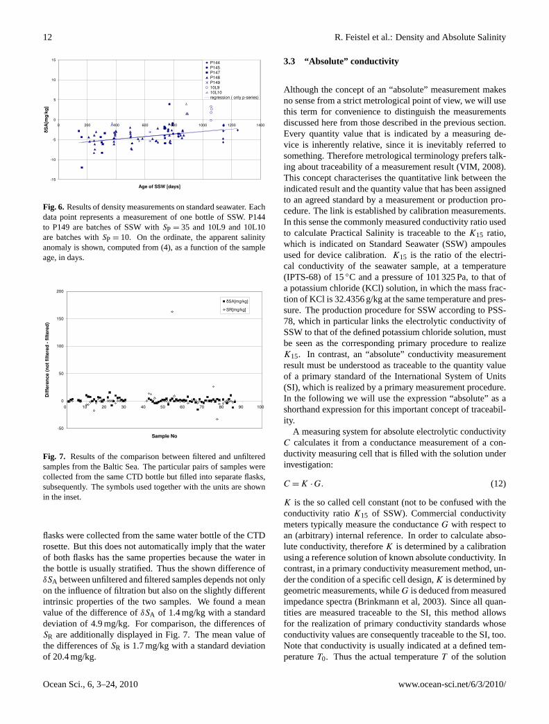
Fig. 6: Results of density measurements on standard seawater. Each data point represents a measurement of one bottle of SSW. P144 to P149 are batches of SSW with SP =35 and 10L9 and 10L10 are batches with SP = 10. On the ordinate, the apparent salinity anomaly is shown, computed from (4), as a function of the sample age, in days. The results of the density measurements of Standard Seawater are shown in Fig. 6. The deviations from zero must be attributed to the stability of the SSW samples and the measuring technique. The calculations refer to the Practical Salinity value given on the ampoule’s label. Practical Salinity measurements could not be done because the SSW samples were used for the calibration of the salinometer. For SSW (only P-series) we found a mean value of the difference �SA of –4.2 mg/kg with a standard deviation of 2.1 mg/kg. There is a slight dependence on the age of the sample. The related regression is line is

�SA /(mg/kg) = 0.0032 d – 6.1453, (11) where d is the age of the samples in days. For SSW (10L-series) the distribution and number of measurements was inadequate for reliable regression results to be obtained. Measurements of the density were done by means of a densitometer DMA 5000 (Anton Paar, Austria). The device was calibrated daily with air and pure water. Measurements of the density and salinity were carried out at the same time as soon as possible after collecting the

Fig. 6. Results of density measurements on standard seawater. Eachdata point represents a measurement of one bottle of SSW. P144to P149 are batches of SSW withSP = 35 and 10L9 and 10L10are batches withSP = 10. On the ordinate, the apparent salinityanomaly is shown, computed from (4), as a function of the sampleage, in days.

-50

0

50

100

150

200

0 10 20 30 40 50 60 70 80 90 100

Sample No

Diff

eren

ce (n

ot fi

ltere

d - f

ilter

ed)

�SA[mg/kg]

SR[mg/kg]

Fig: 7: Results of the comparison between filtered and unfiltered samples from the Baltic Sea. The particular pairs of samples were collected from the same CTD bottle but filled into separate flasks, subsequently. The symbols used together with the units are shown in the inset.

3.3 “Absolute” Conductivity Although the concept of an “absolute” measurement makes no sense from a strict metrological point of view, we will use this term for convenience to distinguish the measurements discussed here from those described in the previous section. Every quantity value that is indicated by a measuring device is inherently relative, since it is inevitably referred to something. Therefore metrological terminology prefers talking about traceability of a measurement result (VIM, 2008). This concept characterises the quantitative link between the indicated result and the quantity value that has been assigned to an agreed standard by a measurement or production procedure. The link is established by calibration measurements. In this sense the commonly measured conductivity ratio used to calculate practical salinity is traceable to the K15 ratio, which is indicated on Standard Seawater (SSW) ampoules used for device calibration. K15 is the ratio of the electrical conductivity of the seawater sample, at a temperature (IPTS-68) of 15 °C and a pressure of 101325 Pa, to that of a potassium chloride (KCl) solution, in which the mass fraction of KCl is 32.4356 g/kg at the same temperature and pressure. The production procedure for SSW according to PSS-78, which in particular links the electrolytic conductivity of SSW to that of the defined potassium chloride solution, must be seen as the corresponding primary procedure to realize K15. In contrast, an “absolute” conductivity measurement result must be understood as traceable to the quantity value of a primary standard of the International System of Units (SI), which is realized by a primary measurement procedure. In the following we will use the expression “absolute” as a shorthand expression for this important concept of traceability.

Fig. 7. Results of the comparison between filtered and unfilteredsamples from the Baltic Sea. The particular pairs of samples werecollected from the same CTD bottle but filled into separate flasks,subsequently. The symbols used together with the units are shownin the inset.

flasks were collected from the same water bottle of the CTDrosette. But this does not automatically imply that the waterof both flasks has the same properties because the water inthe bottle is usually stratified. Thus the shown difference ofδSA between unfiltered and filtered samples depends not onlyon the influence of filtration but also on the slightly differentintrinsic properties of the two samples. We found a meanvalue of the difference ofδSA of 1.4 mg/kg with a standarddeviation of 4.9 mg/kg. For comparison, the differences ofSR are additionally displayed in Fig. 7. The mean value ofthe differences ofSR is 1.7 mg/kg with a standard deviationof 20.4 mg/kg.

3.3 “Absolute” conductivity

Although the concept of an “absolute” measurement makesno sense from a strict metrological point of view, we will usethis term for convenience to distinguish the measurementsdiscussed here from those described in the previous section.Every quantity value that is indicated by a measuring de-vice is inherently relative, since it is inevitably referred tosomething. Therefore metrological terminology prefers talk-ing about traceability of a measurement result (VIM, 2008).This concept characterises the quantitative link between theindicated result and the quantity value that has been assignedto an agreed standard by a measurement or production pro-cedure. The link is established by calibration measurements.In this sense the commonly measured conductivity ratio usedto calculate Practical Salinity is traceable to theK15 ratio,which is indicated on Standard Seawater (SSW) ampoulesused for device calibration.K15 is the ratio of the electri-cal conductivity of the seawater sample, at a temperature(IPTS-68) of 15◦C and a pressure of 101 325 Pa, to that ofa potassium chloride (KCl) solution, in which the mass frac-tion of KCl is 32.4356 g/kg at the same temperature and pres-sure. The production procedure for SSW according to PSS-78, which in particular links the electrolytic conductivity ofSSW to that of the defined potassium chloride solution, mustbe seen as the corresponding primary procedure to realizeK15. In contrast, an “absolute” conductivity measurementresult must be understood as traceable to the quantity valueof a primary standard of the International System of Units(SI), which is realized by a primary measurement procedure.In the following we will use the expression “absolute” as ashorthand expression for this important concept of traceabil-ity.

A measuring system for absolute electrolytic conductivityC calculates it from a conductance measurement of a con-ductivity measuring cell that is filled with the solution underinvestigation:

C = K ·G. (12)

K is the so called cell constant (not to be confused with theconductivity ratioK15 of SSW). Commercial conductivitymeters typically measure the conductanceG with respect toan (arbitrary) internal reference. In order to calculate abso-lute conductivity, thereforeK is determined by a calibrationusing a reference solution of known absolute conductivity. Incontrast, in a primary conductivity measurement method, un-der the condition of a specific cell design,K is determined bygeometric measurements, whileG is deduced from measuredimpedance spectra (Brinkmann et al, 2003). Since all quan-tities are measured traceable to the SI, this method allowsfor the realization of primary conductivity standards whoseconductivity values are consequently traceable to the SI, too.Note that conductivity is usually indicated at a defined tem-peratureT0. Thus the actual temperatureT of the solution

Ocean Sci., 6, 3–24, 2010 www.ocean-sci.net/6/3/2010/

R. Feistel et al.: Density and Absolute Salinity 13

during the measurement is also measured and the measuredconductivity value is corrected toT0.

In the present study we used the primary measurementmethod of the Physikalisch-Technische Bundesanstalt (PTB)(Brinkmann et al, 2003) to measure the absolute conductiv-ity CS of three samples from stations 361, ABB and 213,Fig. 5. After arrival, the samples were stored under cold anddark conditions. Prior to measurement the samples and theconductivity measuring cell were brought to a set tempera-ture of 15◦C (ITS-90) over night in a temperature bath. Weadditionally measured the absolute conductivitiesCSSW ofIAPSO SSW/P-series (batch P149) and 10L10-series (Prac-tical Salinity 9.926, dated 14 June 2006) and calculated theconductivity ratio

R15=CS

CSSWK15 (13)

of the samples under investigation in order to scale the abso-lute conductivity measurement results to PSS-78.K15 ratioswere taken from the SSW ampoules (0.99984 for P-seriesand 0.31712 for L10-series). Conductivity values have beenlinearly corrected to 15◦C (IPTS-68) using a temperature co-efficient of 1.97%/K. Finally we calculated Practical Salinityfrom the PSS-78 formula (Perkin and Lewis, 1980). The un-certainty of the absolute conductivity results includes contri-butions from the determination of temperature, conductanceand the cell constant, and accounts for the statistical spreadof the indicated values. Uncertainty propagation was calcu-lated according to GUM (2008).

3.4 High-accuracy density measurements

Highly accurate density measurements at the PTB Braun-schweig were performed for comparison with an oscillation-type density meter (Anton Paar DMA 5000) using a substi-tution method (Wolf, 2008). In a substitution method thesample to be measured and a reference sample are measuredalternately several times. This method decreases the mea-surement uncertainty considerably as contributions to the un-certainty are mostly correlated and thus vanish when lookingfor the difference between sample and reference.

The reference liquid was ultra pure degassed water. Thedeviation of its density from seawater is below 3%; thus,a very good correlation of the measurements performed onseawater and on ultra pure water is obtained provided thatthe handling of the samples is the same. The water we usedwas de-ionised reverse osmosis water (Milli-Q water (Milli-pore, USA)) with a resistance of 18.2 M� cm and total or-ganic carbon of less than 10×10−9 immediately after purifi-cation. It was made from Braunschweig tap water. The ref-erence density value was taken from the IAPWS-95 formu-lation (Wagner and Pruß, 2002). A correction was made forthe isotopic composition. This was measured to be−8.5δ‰for 18O and−59δ‰ for D compared to Vienna Standard

Mean Ocean Water. Thus, the density reference value forthis Braunschweig tap water is 999.0996 kg/m3 at 15◦C.

An uncorrelated uncertainty contribution is given bythe reproducibility of the device measurement temperature1treproducibility; it was measured to be below 3 mK. Anotheruncertainty contribution arises from the deviation of the de-vice measurement temperature1tdevice from the absolutetemperature. This can be expressed as a calibration uncer-tainty of the measurement temperature. With our device1tdevice was measured to be 0 mK at 15◦C and−5 mK at25◦C. The uncertainty of individual temperature measure-ments is± 5 mK. Typical temperature deviations for otherdevices of the same type are 20 mK. The two temperaturedeviations act in a different way for seawater and for ultrapure water, as their effect on density is given by multiplyingwith the thermal expansion coefficientγ which is differentfor seawater and for ultra pure water:

ρpure water measured=

ρpure water(1+γpure water measured(1tdevice+1treproducibility))

ρseawater measured=

ρseawater(1+γseawater measured(1tdevice+1treproducibility)).

Here,ρpure water measuredandρseawater measuredare the densitiesindicated by the measuring device, whereasρpure waterandρseawaterdenote the real densities.

A third uncorrelated uncertainty contribution is caused bythe different handling of the samples concerning its gas con-tent. The ultra pure water is degassed and will remain de-gassed during the measurement, whereas the seawater is sat-urated with air. The gas content is determined by the storagetemperature of the seawater; during the short time the sam-ple is cooled or heated to the measuring temperature (about15 min) no new equilibration will occur. Thus, the storagetemperature affects the density by the gas content. This ef-fect can be reduced by storing the samples at well controlledreproducible conditions. In our measurements we stored thesamples at refrigerator temperatures and warmed them up toroom temperature over night before measuring. The contri-bution of this handling to the combined uncertainty (GUM,2008) is not investigated up to now and, thus, estimated to berectangular with a halfwidth of 0.5 ppm.

3.5 Ion chromatography

The mass fractions of chloride, bromide and sulphate of thesamples 361, ABB and 213 were determined by means of ionchromatography. For validation purposes the mass fractionsof the same anions were measured in a P149 SSW sample.The P149 results for chloride and sulphate were compared toearlier results on sample P149 determined also by ion chro-matography but using a different instrumental configuration.

www.ocean-sci.net/6/3/2010/ Ocean Sci., 6, 3–24, 2010

14 R. Feistel et al.: Density and Absolute Salinity

The ion chromatography system used here consisted of aMetrohm 881 Compact IC pro (Metrohm, Switzerland) witha Metrosep A Supp 5 column. The eluent was 3.2 mmol/Lsodium carbonate plus 1 mmol/L sodium hydrogen carbon-ate.

All solutions were prepared gravimetrically using Milli-Qwater (Millipore, USA). All seawater samples were dilutedprior to injection. The calibration solutions were preparedfrom certified standard solutions delivered by Fluka (Fluka,Switzerland). The mass fractions as specified by the manu-facturer are for:

chloride:wCl = 1003±3 mg/kgsulphate:wSO4 = 1006±8 mg/kgbromide:wBr = 1003±4 mg/kg.

Calibration solutions containing similar mass fractions of an-ions as the seawater samples were prepared from the stan-dards. Three series of measurements, each using freshly pre-pared sample dilutions were generated for chloride, sulphateand bromide, respectively. Mean values of the mass frac-tions are reported from these measurements in Table 6. Therelative expanded uncertainties (coverage factork = 2) are0.5% for chloride, 0.8% for sulphate and 1% for bromide.The main contributions to the measurement uncertainty arefrom the mass fractions of the certified standard solutions andfrom the preparation of the sample and calibration solution,respectively, by dilution.

4 Results

4.1 Parameterisation of Absolute Salinity

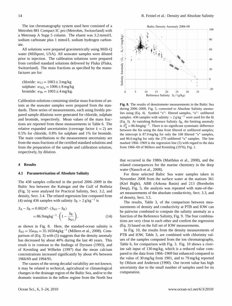
The 438 samples collected in the period 2006–2009 in theBaltic Sea between the Kattegat and the Gulf of Bothnia(Fig. 5) were analysed for Practical Salinity, Sect. 3.2, anddensity, Sect. 3.4. The related regression line computed from(4) using 436 samples with salinitySR > 2 g kg−1 is

SA −SR = 0.00247·(SSO−SR)

= 86.9mgkg−1·

(1−

SR

SSO

), (14)

as shown in Fig. 8. Here, the standard-ocean salinity isSSO= 35uPS= 35.16504gkg−1 (Millero et al., 2008). Com-parison of (Eq. 3) with (5) suggests that the density anomalyhas decreased by about 40% during the last 40 years. Thisresult is in contrast to the findings of Dyrssen (1993), andof Kremling and Wilhelm (1997) that the mean calciumconcentrations increased significantly by about 4% between1966/69 and 1994/95.

The causes of the strong decadal variability are not known;it may be related to technical, agricultural or climatologicalchanges in the drainage region of the Baltic Sea, and/or to thedramatic transition in the inflow regime from the North Sea

0 5 10 15 20 25 30 35-20

0

20

40

60

80

100

Salin

ity A

nom

aly

( S

A -

S R) /

(m

g/kg

)

Reference Salinity SR / (g/kg)

Baltic Density Anomaly 2006-09

1966 - 1969uuu

x

x

x

uuu

u

uu

xxx

xx

xuuuuu

uuuuuuuxxxxxxuuuuuuuuuu

uu

u

u

u

uu

u

u

uu

uu

u

uu

xx

x

xxx

x

xx

x

x

x

xx

x

xxx

x

u

u

u

uxx

xx

x

u

u

uu

uuuu

xxxx

xxxx

u

uuuuu

uxu

x

u

x

u

xuxu

x

uxu

x

u

x

u

x

ux

u

x

u

x

u

x

u

x

u

xu

x

ux

u

x

uxux

ux

ux

uxu

xux

ux

u

xux

ux

uuuu

uuuuuuuuu

u

uu

u

uu u

u

uuuu uuuuu

uuuuuu

uuuuu

uu

u

u

u

uuuu

u

uuu

uu

uuux

x

u

xux

x

x

ux

uxx

x

ux u

x

x xux uxx

x

ux

uxxxuxuxxxu

x

u

xxx u

x

x

ux ux

x

x

uxux

x

xuxux

x

x

uxuxx

xux

u

xx

x

uxxuxxuxxux

x u

x

uuxx

u

x

x

u

xx

uxx

u

xx

uxx

uxx uxx

uxx

u

u

u

u

uu

uu

uu

ux uux

x

xxu

ux

u

x

uuxu

ux

uu

x

u

u

x

uux

u

uu

u uu

u

u

uuu

u u

u

u

u

uu

uu u

u

uu

uuu

u

u

u

u

u

u

u

u

u

u

u

uuuu

uu

uu u uuu

2006 - 2009

Fig. 8: The results of densitometer measurements in the Baltic Sea during 2006-2009, Fig. 5, converted to Absolute Salinity anomalies using eq. (4). Symbol “x”: filtered samples, “u”: unfiltered samples. 436 samples with salinity > 2 g kg –1 were used for the fit (14). At vanishing Reference Salinity SR, the limiting anomaly is 10

A kgmg8.86 −=S . There is no significant systematic difference between the fits using the data from filtered or unfiltered samples; the intercept is 87.0 mg/kg for only the 168 filtered “x” samples, and 86.6 mg/kg for only the 270 unfiltered “u” samples. The line marked 1966-1969 is the regression line (5) with regard to the data from 1966-69 of Millero and Kremling (1976), Fig. 1.

For three selected Baltic Sea water samples taken in November 2008 from the surface water at the stations 361 (Kiel Bight), ABB (Arkona Basin) and 213 (Bornholm Deep), Fig. 5, the analysis was repeated with state-of-the-art measurements of the absolute conductivity, section 3.3, and of density, section 3.5. Table 2: Independent PTB measurements of conductivity and density of Baltic surface water at the selected stations 361, ABB and 213, Fig. 5, compared with the IOW data for density and Practical Salinity. All values are given at 15 °C and atmospheric pressure, except IOW density which was measured at 20 °C. Values for SA were computed from the related density by means of (3). Note that the effect of temperature on density is automatically removed when calculating the “density salinity”, which is reported as SA. Related expanded uncertainties (coverage factor 2) are given below the values

Fig. 8. The results of densitometer measurements in the Baltic Seaduring 2006–2009, Fig. 5, converted to Absolute Salinity anoma-lies using (Eq. 4). Symbol “x”: filtered samples, “u”: unfilteredsamples. 436 samples with salinity> 2 g kg−1 were used for the fit(Eq. 3). At vanishing Reference SalinitySR, the limiting anomalyis S0

A = 86.8mgkg−1. There is no significant systematic differencebetween the fits using the data from filtered or unfiltered samples;the intercept is 87.0 mg/kg for only the 168 filtered “x” samples,and 86.6 mg/kg for only the 270 unfiltered “u” samples. The linemarked 1966–1969 is the regression line (5) with regard to the datafrom 1966–69 of Millero and Kremling (1976), Fig. 1.

that occurred in the 1980s (Matthaus et al., 2008), and therelated consequences for the marine chemistry in the deepwater (Nausch et al., 2008).

For three selected Baltic Sea water samples taken inNovember 2008 from the surface water at the stations 361(Kiel Bight), ABB (Arkona Basin) and 213 (BornholmDeep), Fig. 5, the analysis was repeated with state-of-the-art measurements of the absolute conductivity, Sect. 3.3, andof density, Sect. 3.5.

The results, Table 3, of the comparison between mea-surements of density and conductivity at PTB and IOW canbe pairwise combined to compute the salinity anomaly as afunction of the Reference Salinity, Fig. 9. The four combina-tions are very close to each other and confirm the regression(Eq. 3) based on the full set of IOW measurements.

In Fig. 10, the results from the density measurements ofPTB and IOW, Table 3, are combined with chlorinity val-ues of the samples computed from the ion chromatography,Table 6, for comparison with Fig. 3. Fig. 10 shows a river-ine salt input of 130 mg/kg, which is a reduced value com-pared to the data from 1966–1969 but enhanced compared tothe value of 30 mg/kg from 1901, and to 79 mg/kg reportedby Ohlson and Anderson (1990). Our recent value has highuncertainty due to the small number of samples used for itscomputation.

Ocean Sci., 6, 3–24, 2010 www.ocean-sci.net/6/3/2010/

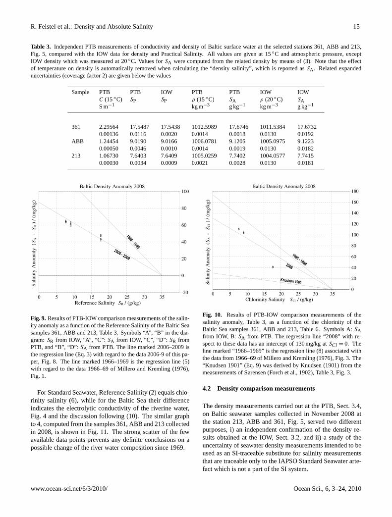
R. Feistel et al.: Density and Absolute Salinity 15

Table 3. Independent PTB measurements of conductivity and density of Baltic surface water at the selected stations 361, ABB and 213,Fig. 5, compared with the IOW data for density and Practical Salinity. All values are given at 15◦C and atmospheric pressure, exceptIOW density which was measured at 20◦C. Values forSA were computed from the related density by means of (3). Note that the effectof temperature on density is automatically removed when calculating the “density salinity”, which is reported asSA . Related expandeduncertainties (coverage factor 2) are given below the values

Sample PTBC (15◦C)S m−1

PTBSP

IOWSP

PTBρ (15◦C)kg m−3

PTBSAg kg−1

IOWρ (20◦C)kg m−3

IOWSAg kg−1

361 2.295640.00136

17.54870.0116

17.54380.0020

1012.59890.0014

17.67460.0018

1011.53840.0130

17.67320.0192

ABB 1.244540.00050

9.01900.0046

9.01660.0010

1006.07810.0014

9.12050.0019

1005.09750.0130

9.12230.0182

213 1.067300.00030

7.64030.0034

7.64090.0009

1005.02590.0021

7.74020.0028

1004.05770.0130

7.74150.0181

Sample PTB C (15 °C)

S m–1

PTB SP

IOW SP

PTB � (15 °C)

kg m–3

PTB SA

g kg–1

IOW � (20 °C)

kg m–3

IOW SA

g kg–1 361 2.29564

0.00136 17.5487 0.0116

17.5438 0.0020

1012.5989 0.0014

17.6746 0.0018

1011.5384 0.0130

17.6732 0.0192

ABB 1.24454 0.00050

9.0190 0.0046

9.0166 0.0010

1006.0781 0.0014

9.1205 0.0019

1005.0975 0.0130

9.1223 0.0182

213 1.06730 0.00030

7.6403 0.0034

7.6409 0.0009

1005.0259 0.0021

7.7402 0.0028

1004.0577 0.0130

7.7415 0.0181

The results, Table 2, of the comparison between measurements of density and conductivity at PTB and IOW can be pairwise combined to compute the salinity anomaly as a function of the Reference Salinity, Fig. 9. The four combinations are very close to each other and confirm the regression (14) based on the full set of IOW measurements.

0 5 10 15 20 25 30 35-20

0

20

40

60

80

100

Salin

ity A

nom

aly

( S

A -

S R) /

(m

g/kg

)

Reference Salinity SR / (g/kg)

Baltic Density Anomaly 2008

1966 - 19692006 - 2009

A

AA

B

BB

C

CC

D

D

D

Fig. 9: Results of PTB-IOW comparison measurements of the salinity anomaly as a function of the Reference Salinity of the Baltic Sea samples 361, ABB and 213, Table 2. Symbols “A”, “B”: SR from IOW, “A”, “C”: SA from IOW, “C”, “D”: SR from PTB, and “B”, “D”: SA from PTB. The line marked 2006-2009 is the regression line (14) with regard to the data 2006-9 of this paper, Fig. 8. The line marked 1966-1969 is the regression line (5) with regard to the data 1966-69 of Millero and Kremling (1976), Fig. 1.

Fig. 9. Results of PTB-IOW comparison measurements of the salin-ity anomaly as a function of the Reference Salinity of the Baltic Seasamples 361, ABB and 213, Table 3. Symbols “A”, “B” in the dia-gram: SR from IOW, “A”, “C”: SA from IOW, “C”, “D”: SR fromPTB, and “B”, “D”: SA from PTB. The line marked 2006–2009 isthe regression line (Eq. 3) with regard to the data 2006-9 of this pa-per, Fig. 8. The line marked 1966–1969 is the regression line (5)with regard to the data 1966–69 of Millero and Kremling (1976),Fig. 1.

For Standard Seawater, Reference Salinity (2) equals chlo-rinity salinity (6), while for the Baltic Sea their differenceindicates the electrolytic conductivity of the riverine water,Fig. 4 and the discussion following (10). The similar graphto 4, computed from the samples 361, ABB and 213 collectedin 2008, is shown in Fig. 11. The strong scatter of the fewavailable data points prevents any definite conclusions on apossible change of the river water composition since 1969.

In Fig. 10, the results from the density measurements of PTB and IOW, Table 2, are combined with chlorinity values of the samples computed from the ion chromatography, Table 5, for comparison with Fig. 3. Fig. 10 shows a riverine salt input of 130 mg/kg, which is a reduced value compared to the data from 1966-1969 but enhanced compared to the value of 30 mg/kg from 1901, and to 79 mg/kg reported by Ohlson and Anderson (1990). Our recent value has high uncertainty due to the small number of samples used for its computation.

0 5 10 15 20 25 30 350

20

40

60

80

100

120

140

160

180

Salin

ity A

nom

aly

( S A

- S C

l) /

(mg/

kg)

Chlorinity Salinity SCl / (g/kg)

Baltic Density Anomaly 2008

1966 - 1969

Knudsen 1901

A

A

A

B

BB

2008

Fig. 10: Results of PTB-IOW comparison measurements of the salinity anomaly, Table 2, as a function of the chlorinity of the Baltic Sea samples 361, ABB and 213, Table 5. Symbols “A“: SA from IOW, “B: SA from PTB. The regression line “2008” with respect to these data has an intercept of 130 mg/kg at SCl = 0. The line marked “1966-1969” is the regression line (8) associated with the data from 1966-69 of Millero and Kremling (1976), Fig. 3. The “Knudsen 1901” equation (9) was derived by Knudsen (1901) from the measurements of Sørensen (Forch et al. 1902), Table t2.0, Fig. 3.

For Standard Seawater, Reference Salinity (2) equals chlorinity salinity (6), while for the Baltic Sea their difference indicates the electrolytic conductivity of the riverine water, Fig. 4 and the discussion following (10). The similar graph to 4, computed from the samples 361, ABB and 213 collected in 2008, is shown in Fig. 11. The strong scatter of the few available data points prevents any definite conclusions on a possible change of the river water composition since 1969.

Fig. 10. Results of PTB-IOW comparison measurements of thesalinity anomaly, Table 3, as a function of the chlorinity of theBaltic Sea samples 361, ABB and 213, Table 6. Symbols A:SAfrom IOW, B: SA from PTB. The regression line “2008” with re-spect to these data has an intercept of 130 mg/kg atSCl = 0. Theline marked “1966–1969” is the regression line (8) associated withthe data from 1966–69 of Millero and Kremling (1976), Fig. 3. The“Knudsen 1901” (Eq. 9) was derived by Knudsen (1901) from themeasurements of Sørensen (Forch et al., 1902), Table 3, Fig. 3.

4.2 Density comparison measurements

The density measurements carried out at the PTB, Sect. 3.4,on Baltic seawater samples collected in November 2008 atthe station 213, ABB and 361, Fig. 5, served two differentpurposes, i) an independent confirmation of the density re-sults obtained at the IOW, Sect. 3.2, and ii) a study of theuncertainty of seawater density measurements intended to beused as an SI-traceable substitute for salinity measurementsthat are traceable only to the IAPSO Standard Seawater arte-fact which is not a part of the SI system.

www.ocean-sci.net/6/3/2010/ Ocean Sci., 6, 3–24, 2010

16 R. Feistel et al.: Density and Absolute Salinity

0 5 10 15 20 25 30 35 40-50

-40

-30

-20

-10

0

10

20

30

40

50

Salin

ity A

nom

aly

( S R

- S C

l) /

(mg/

kg)

Chlorinity Salinity SCl / (g/kg)

Salinity-Chlorinity Anomaly 2008

A

A

A

B

BB

1966 - 1969

Fig. 11: Deviation between Reference Salinity (2), SR, from Table 2, and chlorinity salinity (6), SCl, from Table 5, of the Baltic Sea samples 361, ABB and 213, compared with the regression line “1966-1969” with respect to Kremling’s data collected between 1966 and 1969, Fig. 4. The deviation from the abscissa quantifies the conductivity of the riverine water. Symbols “A” with Practical Salinity from the IOW, “B” from the PTB.

4.2 Density Comparison Measurements The density measurements carried out at the PTB, section 3.4, on Baltic seawater samples collected in November 2008 at the station 213, ABB and 361, Fig. 5, served two different purposes, i) an independent confirmation of the density results obtained at the IOW, section 3.2, and ii) a study of the uncertainty of seawater density measurements intended to be used as an SI-traceable substitute for salinity measurements that are traceable only to the IAPSO Standard Seawater artefact which is not a part of the SI system. The results of the PTB density measurements are reported in detail in Tables 3, 4 and Figs. 12 - 15. Expanded uncertainties for seawater densities are estimated to be in the range of 1-2 mg/m³, the standard deviation of pure-water measurements is even below 1 mg/m³. The agreement of the PTB results with IOW data is excellent, as seen from the Absolute Salinity results shown in Table 2 and Figs. 9 - 10. The lowering of the Baltic salinity anomaly in 2006-9 compared to 1966-69 derived from IOW data is confirmed by the PTB determinations.

Fig. 11. Deviation between Reference Salinity (2),SR, from Ta-ble 3, and chlorinity salinity (6),SCl , from Table 6, of the BalticSea samples 361, ABB and 213, compared with the regression line“1966–1969” with respect to Kremling’s data collected between1966 and 1969, Fig. 4. The deviation from the abscissa quantifiesthe conductivity of the riverine water. Symbols A with PracticalSalinity from the IOW, B from the PTB.

The results of the PTB density measurements are reportedin detail in Tables 4, 5 and Figs. 12–15. Expanded uncertain-ties for seawater densities are estimated to be in the rangeof 1–2 mg/m3, the standard deviation of pure-water measure-ments is even below 1 mg/m3.

The agreement of the PTB results with IOW data is ex-cellent, as seen from the Absolute Salinity results shown inTable 3 and Figs. 9–10. The lowering of the Baltic salinityanomaly in 2006-9 compared to 1966–69 derived from IOWdata is confirmed by the PTB determinations.

The typical uncertainties displayed in Figs. 12–14 forBaltic Seawater apply similarly to Standard Seawater;Fig. 15; the measurement method is not modified for brack-ish salinities. The uncertainties of salinitiesSA computedfrom the PTB density measurements, Table 3, are compara-ble to those of the Practical Salinity measured at IOW withconventional conductivity methods. Thus, the results pre-sented here support the idea of measuring salinity by meansof SI-traceable density.

Another important aspect of the substitution method usedhere is the automatic consistency with IAPWS-95 densitiesof pure water. This permits the computation of the saline partof the specific volume of seawater (IAPWS, 2008) from mea-sured seawater densities without additional loss of accuracy.

ABB -3 3.4E-04 18 0.00016893 2.4E-04 22 ABB -8 5.0E-04 14 0.00016893 4.5E-04 18 ABB -2 3.1E-04 20 0.00016893 4.6E-04 22 361-1 4.3E-04 18 0.0001847 2.2E-04 22 361-9 3.1E-04 18 0.0001847 3.0E-04 22 361-2 7.5E-04 20 0.0001847 2.9E-04 20

P151-1 7.5E-04 18 0.00016628 4.7E-04 22 P151-2 4.8E-04 18 0.00016628 1.7E-04 22 P151-3 5.5E-04 18 0.00016893 3.8E-04 22 P151-4 2.6E-04 18 0.00016893 3.0E-04 22

1005.022

1005.023

1005.024

1005.025

1005.026

1005.027

1005.028

1005.029

1005.030

213-1 213-3 213-9 213-2

Den

sity

in k

g/m

³

Bottle

t = 15�C

Fig. 12: Densities and uncertainties of the different batches, Table 3, of surface water from the Baltic Sea station 213, Fig. 5, measured at the PTB.

1006.074

1006.075

1006.076

1006.077

1006.078

1006.079

1006.080

1006.081

1006.082

1006.083

ABB-1 ABB-3 ABB-8 ABB-2

Den

sity

in k

g/m

³

Bottle

t = 15�C

Fig. 13: Densities and uncertainties of the different batches, Table 3, of surface water from the Baltic Sea station ABB, Fig. 5, measured at the PTB

Fig. 12.Densities and uncertainties of the different batches, Table 4,of surface water from the Baltic Sea station 213, Fig. 5, measuredat the PTB.

ABB -3 3.4E-04 18 0.00016893 2.4E-04 22 ABB -8 5.0E-04 14 0.00016893 4.5E-04 18 ABB -2 3.1E-04 20 0.00016893 4.6E-04 22 361-1 4.3E-04 18 0.0001847 2.2E-04 22 361-9 3.1E-04 18 0.0001847 3.0E-04 22 361-2 7.5E-04 20 0.0001847 2.9E-04 20

P151-1 7.5E-04 18 0.00016628 4.7E-04 22 P151-2 4.8E-04 18 0.00016628 1.7E-04 22 P151-3 5.5E-04 18 0.00016893 3.8E-04 22 P151-4 2.6E-04 18 0.00016893 3.0E-04 22

1005.022

1005.023

1005.024

1005.025

1005.026

1005.027

1005.028

1005.029

1005.030

213-1 213-3 213-9 213-2

Den

sity

in k

g/m

³

Bottle

t = 15�C

Fig. 12: Densities and uncertainties of the different batches, Table 3, of surface water from the Baltic Sea station 213, Fig. 5, measured at the PTB.

1006.074

1006.075

1006.076

1006.077

1006.078

1006.079

1006.080

1006.081

1006.082

1006.083

ABB-1 ABB-3 ABB-8 ABB-2

Den

sity

in k

g/m

³

Bottle

t = 15�C

Fig. 13: Densities and uncertainties of the different batches, Table 3, of surface water from the Baltic Sea station ABB, Fig. 5, measured at the PTB Fig. 13.Densities and uncertainties of the different batches, Table 4,of surface water from the Baltic Sea station ABB, Fig. 5, measuredat the PTB

4.3 Conductivity comparison measurements

Figure 16 shows the differences between Practical Salinitymeasured at the IOW with a salinometer (Ssal

P ), Sect. 3.2, andPractical Salinity calculated from absolute conductivity mea-surements (Sabs

P ), Sect. 3.3. Zero in Fig. 16 can be taken asa representative forSabs

P , the dots then mark the deviation ofSsal

P with respect toSabsP . The error bars indicate the expanded

(coverage factor 2) uncertainties. Bars with a cross bar arethose ofSsal

P and without cross bars those ofSabsP . They in-

dicate a 95 % degree of confidence for the results. Only thestatistical fluctuation of the internally measured conductanceenters into the uncertainty ofSsal

P , since systematic uncer-tainties are assumed to cancel out by the SSW calibrationprocedure. In an absolute conductivity measurement the ab-solute conductance value of seawater in the measuring cellmust be determined. Its uncertainty therefore enters into theuncertainties ofCS andCSSW in (Eq. 2). This results in alarger uncertainty ofSabs

P as can be seen in Fig. 16.

Ocean Sci., 6, 3–24, 2010 www.ocean-sci.net/6/3/2010/

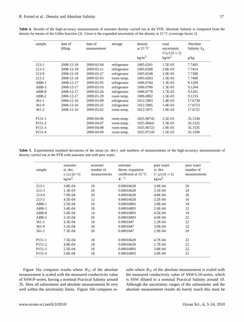
R. Feistel et al.: Density and Absolute Salinity 17

Table 4. Results of the high-accuracy measurements of seawater density carried out at the PTB. Absolute Salinity is computed from thedensity by means of the Gibbs function (3). Given is the expanded uncertainty of the density at 15◦C (coverage factor 2).

sample date offilling

date ofmeasurement

storage densityat 15◦C

totaluncertaintyU (ρ) (k = 2)

AbsoluteSalinitySA

kg/m3 kg/m3 g/kg

213-1 2008-12-18 2009-02-04 refrigerator 1005.0261 1.5E-03 7.7405213-3 2008-12-18 2009-03-11 refrigerator 1005.0268 2.8E-03 7.7414213-9 2008-12-18 2009-03-27 refrigerator 1005.0248 2.0E-03 7.7388213-2 2008-12-18 2009-02-03 room temp. 1005.0263 1.5E-03 7.7408ABB-1 2008-12-17 2009-02-05 refrigerator 1006.0784 1.3E-03 9.1209ABB-3 2008-12-17 2009-03-10 refrigerator 1006.0780 1.3E-03 9.1204ABB-8 2008-12-17 2009-03-26 refrigerator 1006.0778 1.7E-03 9.1201ABB-2 2008-12-17 2009-01-29 room temp. 1006.0802 1.5E-03 9.1233361-1 2008-12-16 2009-03-09 refrigerator 1012.5983 1.4E-03 17.6738361-9 2008-12-16 2009-03-25 refrigerator 1012.5995 1.4E-03 17.6753361-2 2008-12-16 2009-02-02 room temp. 1012.5971 1.9E-03 17.6722

P151-1 2009-04-06 room temp. 1025.96745 2.2E-03 35.1538P151-2 2009-04-07 room temp. 1025.96641 1.3E-03 35.1525P151-3 2009-04-08 room temp. 1025.96722 1.9E-03 35.1535P151-4 2009-04-09 room temp. 1025.97145 1.5E-03 35.1590

Table 5. Experimental standard deviations of the mean (st. dev.) and numbers of measurements of the high-accuracy measurements ofdensity carried out at the PTB with seawater and with pure water.

seawater seawater seawater pure water pure watersample st. dev.

u (ρ) (k=1)number ofmeasurements

therm. expansioncoefficient at 15◦C

st. dev.U (ρ) (k = 2)

number ofmeasurements

kg/m3 K−1 kg/m3

213-1 3.8E-04 16 0.00016628 3.9E-04 20213-3 1.3E-03 20 0.00016628 3.1E-04 24213-9 7.0E-04 20 0.00016628 4.8E-04 26213-2 4.5E-04 12 0.00016628 3.2E-04 16ABB-1 2.5E-04 16 0.00016893 3.8E-04 18ABB-3 3.4E-04 18 0.00016893 2.4E-04 22ABB-8 5.0E-04 14 0.00016893 4.5E-04 18ABB-2 3.1E-04 20 0.00016893 4.6E-04 22361-1 4.3E-04 18 0.0001847 2.2E-04 22361-9 3.1E-04 18 0.0001847 3.0E-04 22361-2 7.5E-04 20 0.0001847 2.9E-04 20

P151-1 7.5E-04 18 0.00016628 4.7E-04 22P151-2 4.8E-04 18 0.00016628 1.7E-04 22P151-3 5.5E-04 18 0.00016893 3.8E-04 22P151-4 2.6E-04 18 0.00016893 3.0E-04 22

Figure 16a compares results whereR15 of the absolutemeasurement is scaled with the measured conductivity valueof SSW/P-series, having a nominal Practical Salinity around35. Here all salinometer and absolute measurements fit verywell within the uncertainty limits. Figure 16b compares re-

sults whereR15 of the absolute measurement is scaled withthe measured conductivity value of SSW/L10-series, whichis SSW diluted to a nominal Practical Salinity around 10.Although the uncertainty ranges of the salinometer and theabsolute measurement results do barely touch this must be

www.ocean-sci.net/6/3/2010/ Ocean Sci., 6, 3–24, 2010

18 R. Feistel et al.: Density and Absolute Salinity

1012.594

1012.595

1012.596

1012.597

1012.598

1012.599

1012.600

1012.601

361-1 361-9 361-2

Den

sity

in k

g/m

³

Bottle

t = 15�C

Fig. 14: Densities and uncertainties of the different batches, Table 3, of surface water from the Baltic Sea station 361, Fig. 5, measured at the PTB.

1025.965

1025.966

1025.967

1025.968

1025.969

1025.970

1025.971

1025.972

1025.973

P151-1 P151-2 P151-3 P151-4

Den

sity

in k

g/m

³

Bottle

t = 15�C

Fig. 15: Densities and uncertainties of the different batches of IAPSO Standard Seawater, measured at the PTB. The outlier of bottle P151-4 is not attributed to a measurement effect but should be interpreted as an indication for evaporation of water caused by an imperfect sealing of the bottle.

4.3 Conductivity Comparison Measurements Fig. 16 shows the differences between Practical Salinity measured at the IOW with a salinometer ( sal

PS ), section 3.2, and Practical Salinity calculated from absolute conductivity

measurements ( absPS ), section 3.3. Zero in Fig. 16 can be taken as a representative for abs

PS , the

dots then mark the deviation of salPS with respect to abs

PS . The error bars indicate the expanded

Fig. 14.Densities and uncertainties of the different batches, Table 4,of surface water from the Baltic Sea station 361, Fig. 5, measuredat the PTB.

1012.594

1012.595

1012.596

1012.597

1012.598

1012.599

1012.600

1012.601

361-1 361-9 361-2

Den

sity

in k

g/m

³

Bottle

t = 15�C

Fig. 14: Densities and uncertainties of the different batches, Table 3, of surface water from the Baltic Sea station 361, Fig. 5, measured at the PTB.

1025.965

1025.966

1025.967

1025.968

1025.969

1025.970

1025.971

1025.972

1025.973

P151-1 P151-2 P151-3 P151-4

Den

sity

in k

g/m

³

Bottle

t = 15�C

Fig. 15: Densities and uncertainties of the different batches of IAPSO Standard Seawater, measured at the PTB. The outlier of bottle P151-4 is not attributed to a measurement effect but should be interpreted as an indication for evaporation of water caused by an imperfect sealing of the bottle.

4.3 Conductivity Comparison Measurements Fig. 16 shows the differences between Practical Salinity measured at the IOW with a salinometer ( sal

PS ), section 3.2, and Practical Salinity calculated from absolute conductivity

measurements ( absPS ), section 3.3. Zero in Fig. 16 can be taken as a representative for abs

PS , the

dots then mark the deviation of salPS with respect to abs

PS . The error bars indicate the expanded

Fig. 15. Densities and uncertainties of the different batches ofIAPSO Standard Seawater, measured at the PTB. The outlier of bot-tle P151-4 is not attributed to a measurement effect but should beinterpreted as an indication for evaporation of water caused by animperfect sealing of the bottle.

assessed as a significant deviation. This is an unexpectedobservation; we may only speculate here about the reasons.Since PSS-78 is based on Practical Salinity measurements ofSSW at different salt concentrations, scaling with SSW/P-series or L10-series should lead to the same result. The devi-ation may be an indicator that today’s internal scaling of themeasuring device is different to the devices taken to estab-lish PSS-78. Alternatively, e.g., the physical chemical prop-erties of SSW may have slightly changed such that PSS-78cannot be reproduced anymore over the complete scale. Ofcourse, such a far-reaching conclusion can certainly not bedrawn from such a small set of measurements with lackingstatistical significance. Consequently, further investigationis currently ongoing. But based on the present results inthe Baltic Sea measurement range one has to expect an ad-ditional uncertainty contribution to Practical Salinity in theorder of the deviation of about 0.06% to 0.07%. At least theresults demonstrate the necessity of an independent and sta-ble reference for Practical Salinity measurements like the SI.

(coverage factor 2) uncertainties. Bars with a cross bar are those of salPS and without cross

bars those of absPS . They indicate a 95 % degree of confidence for the results. Only the

statistical fluctuation of the internally measured conductance enters into the uncertainty of sal

PS , since systematic uncertainties are assumed to cancel out by the SSW calibration procedure. In an absolute conductivity measurement the absolute conductance value of seawater in the measuring cell must be determined. Its uncertainty therefore enters into the uncertainties of CS and CSSW in eq. (13). This results in a larger uncertainty of abs

PS as can be seen in Fig 16. Fig. 16 a) compares results where R15 of the absolute measurement is scaled with the measured conductivity value of SSW/P-series, having a nominal Practical Salinity around 35. Here all salinometer and absolute measurements fit very well within the uncertainty limits. Fig. 16 b) compares results where R15 of the absolute measurement is scaled with the measured conductivity value of SSW/L10-series, which is SSW diluted to a nominal Practical Salinity around 10. Although the uncertainty ranges of the salinometer and the absolute measurement results do barely touch this must be assessed as a significant deviation. This is an unexpected observation; we may only speculate here about the reasons. Since PSS-78 is based on Practical Salinity measurements of SSW at different salt concentrations, scaling with SSW/P-series or L10-series should lead to the same result. The deviation may be an indicator that today’s internal scaling of the measuring device is different to the devices taken to establish PSS-78. Alternatively, e.g., the physical chemical properties of SSW may have slightly changed such that PSS-78 cannot be reproduced anymore over the complete scale. Of course, such a far-reaching conclusion can certainly not be drawn from such a small set of measurements with lacking statistical significance. Consequently, further investigation is currently ongoing. But based on the present results in the Baltic Sea measurement range one has to expect an additional uncertainty contribution to Practical Salinity in the order of the deviation of about 0.06 % to 0.07 %. At least the results demonstrate the necessity of an independent and stable reference for Practical Salinity measurements like the SI.

-0.02

-0.01

0.00

0.01

0.02

Sample

Ssa

l

P -

Sabs

P

a) scaled with K15

of

IAPSO SSW/P-series

213ABB361

-0.02

-0.01

0.00

0.01

0.02

Sample213ABB

Ssa

l

P -

Sabs

P

b) scaled with K15

of SSW/10L10-series

361

Fig. 16: Deviation of Practical Salinity results sal

PS measured with a salinometer from those

calculated from absolute conductivity measurements absPS . Error bars without cross bars are

related to zero (deviation) and indicate the expanded uncertainty of absPS , while the error bars

with cross bars indicate the expanded uncertainty of salPS . a) Absolute conductivity results

scaled according to eq. (13) using SSW/P-series, b) using SSW/10L10 series.

(coverage factor 2) uncertainties. Bars with a cross bar are those of salPS and without cross

bars those of absPS . They indicate a 95 % degree of confidence for the results. Only the

statistical fluctuation of the internally measured conductance enters into the uncertainty of sal

PS , since systematic uncertainties are assumed to cancel out by the SSW calibration procedure. In an absolute conductivity measurement the absolute conductance value of seawater in the measuring cell must be determined. Its uncertainty therefore enters into the uncertainties of CS and CSSW in eq. (13). This results in a larger uncertainty of abs

PS as can be seen in Fig 16. Fig. 16 a) compares results where R15 of the absolute measurement is scaled with the measured conductivity value of SSW/P-series, having a nominal Practical Salinity around 35. Here all salinometer and absolute measurements fit very well within the uncertainty limits. Fig. 16 b) compares results where R15 of the absolute measurement is scaled with the measured conductivity value of SSW/L10-series, which is SSW diluted to a nominal Practical Salinity around 10. Although the uncertainty ranges of the salinometer and the absolute measurement results do barely touch this must be assessed as a significant deviation. This is an unexpected observation; we may only speculate here about the reasons. Since PSS-78 is based on Practical Salinity measurements of SSW at different salt concentrations, scaling with SSW/P-series or L10-series should lead to the same result. The deviation may be an indicator that today’s internal scaling of the measuring device is different to the devices taken to establish PSS-78. Alternatively, e.g., the physical chemical properties of SSW may have slightly changed such that PSS-78 cannot be reproduced anymore over the complete scale. Of course, such a far-reaching conclusion can certainly not be drawn from such a small set of measurements with lacking statistical significance. Consequently, further investigation is currently ongoing. But based on the present results in the Baltic Sea measurement range one has to expect an additional uncertainty contribution to Practical Salinity in the order of the deviation of about 0.06 % to 0.07 %. At least the results demonstrate the necessity of an independent and stable reference for Practical Salinity measurements like the SI.

-0.02

-0.01

0.00

0.01

0.02

Sample

Ssa

l

P -

Sabs

P

a) scaled with K15

of

IAPSO SSW/P-series

213ABB361

-0.02

-0.01

0.00

0.01

0.02

Sample213ABB

Ssa

l

P -

Sabs

P

b) scaled with K15

of SSW/10L10-series

361

Fig. 16: Deviation of Practical Salinity results sal

PS measured with a salinometer from those

calculated from absolute conductivity measurements absPS . Error bars without cross bars are

related to zero (deviation) and indicate the expanded uncertainty of absPS , while the error bars

with cross bars indicate the expanded uncertainty of salPS . a) Absolute conductivity results

scaled according to eq. (13) using SSW/P-series, b) using SSW/10L10 series.

Fig. 16.Deviation of Practical Salinity resultsSsalP measured with a

salinometer from those calculated from absolute conductivity mea-surementsSabs

P . Error bars without cross bars are related to zero

(deviation) and indicate the expanded uncertainty ofSabsP , while the

error bars with cross bars indicate the expanded uncertainty ofSsalP .

(a) Absolute conductivity results scaled according to (Eq. 2) usingSSW/P-series,(b) using SSW/10L10 series.

4.4 Chemical composition

Table 6 summarizes the results of the ion chromatographymeasurements, Sect. 3.6, together with the expanded uncer-tainties4 (coverage factor 2, GUM 2008). The mass frac-tions of the anions chloride, bromide and sulphate were de-termined in the samples 361, ABB and 213 and in a sam-ple of P149 SSW. In columns 2 and 3 of Table 8 the massfractions of sulphate to chloride and bromide to chloride aregiven. Figs. 18 and 19 show the results graphically. In Fig. 17the mass fractions of sulphate determined in two samplesof P149 SSW are compared. One sample P149 was mea-sured at the same time as the Baltic Sea samples the otherwas measured one year before using a different instrumen-tal configuration (Metrohm 850 professional IC, Metrosep ASupp 4/5 Guard column, Metrohm, Switzerland) and done

4The expanded uncertaintyU defines an interval about the re-sult of the measurement.U is calculated from a combined standarduncertaintyuc and a coverage factork: U = kuc. A coverage fac-tor k = 2, as applied in the publication, corresponds for a normaldistribution to a coverage probability of approximately 95%.

Ocean Sci., 6, 3–24, 2010 www.ocean-sci.net/6/3/2010/

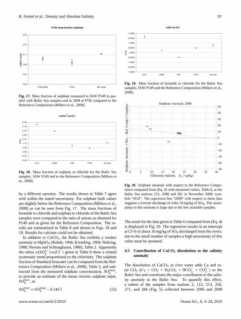
R. Feistel et al.: Density and Absolute Salinity 19

Table 6: Mass fractions of chloride and sulphate measured in SSW P149 in parallel with Baltic Sea samples and in 2008 at PTB, compared to the reference composition (Millero et al., 2008).

Sample P149 this paper

P149 PTB in 2008

reference composition Millero et al. (2008)

Seawater component i

w(i) g kg–1

U (w(i)) g kg–1

w(i) g kg–1

U (w(i)) g kg–1

w(i) g kg–1

U (w(i)) g kg–1

Cl– 19.39 0.04 19.34 0.03 19.35271

SO42– 2.694 0.006 2.702 0.004 2.71235

Table 7: Mass fraction of sulphate to chloride and bromide to chloride for the Baltic Sea samples, the standard seawater sample compared to SSW P149 and to the reference composition (Millero et al., 2008).

Sample w(SO42–)/w(Cl–) w(Br–)/w(Cl–)

213 0.1445 0.003566 ABB 0.1429 0.003425 361 0.1395 0.003351

P149 0.1389 0.003448 Ref. Comp. 0.1390 0.003480

P149 mass fraction sulphate

2.65

2.67

2.69

2.71

2.73

2.75

P149(2008) P149 Ref comp

w(S

O42-

) g

kg

-1

Fig. 17: Mass fraction of sulphate measured in SSW P149 in parallel with Baltic Sea samples and in 2008 at PTB compared to the reference composition (Millero et al., 2008).

Fig. 17. Mass fraction of sulphate measured in SSW P149 in par-allel with Baltic Sea samples and in 2008 at PTB compared to theReference Composition (Millero et al., 2008).

w (SO42-)/w (Cl-)

0.136

0.137

0.138

0.139

0.14

0.141

0.142

0.143

0.144

0.145

s213 sABB s361 P149 ref comp

wi/w

i

Fig. 18: Mass fraction of sulphate to chloride for the Baltic Sea samples. SSW P149 and to the reference composition (Millero et al., 2008).

w (Br-)/w (Cl-)

0.0032

0.00325

0.0033

0.00335

0.0034

0.00345

0.0035

0.00355

0.0036

s213 sABB s361 P149 ref comp

wi/w

i

Fig. 19: Mass fraction of bromide to chloride for the Baltic Sea samples, SSW P149 and the reference composition (Millero et al., 2008). In addition to CaCO3, the Baltic Sea exhibits a weaker anomaly in MgSO4 (Rohde, 1966; Kremling, 1969; Nehring, 1980; Nessim and Schlungbaum, 1980), Table 1. Apparently the

Fig. 18. Mass fraction of sulphate to chloride for the Baltic Seasamples. SSW P149 and to the Reference Composition (Millero etal., 2008).

by a different operator. The results shown in Table 7 agreewell within the stated uncertainty. For sulphate both valuesare slightly below the Reference Composition (Millero et al.,2008) as can be seen from Fig. 17. The mass fractions ofbromide to chloride and sulphate to chloride of the Baltic Seasamples were compared to the ratio of anions as obtained forP149 and as given for the Reference Composition. The re-sults are summarized in Table 8 and shown in Figs. 18 and19. Results for calcium could not be obtained.

In addition to CaCO3, the Baltic Sea exhibits a weakeranomaly in MgSO4 (Rohde, 1966; Kremling, 1969; Nehring,1980; Nessim and Schlungbaum, 1980), Table 2. Apparentlythe ratiosw(SO2−

4 )/w(Cl−) given in Table 8 show a relatedsystematic trend proportional to the chlorinity. The sulphatefraction of Standard Seawater can be computed from the Ref-erence Composition (Millero et al., 2008), Table 2, and sub-tracted from the measured sulphate concentration, SOmeas

4 ,to provide an estimate of the mean riverine sulphate input,SOriver

4 , as

SOriver4 = SOmeas

4 −0.14Cl (15)

w (SO42-)/w (Cl-)

0.136

0.137

0.138

0.139

0.14

0.141

0.142

0.143

0.144

0.145

s213 sABB s361 P149 ref comp

wi/w

i

Fig. 18: Mass fraction of sulphate to chloride for the Baltic Sea samples. SSW P149 and to the reference composition (Millero et al., 2008).

w (Br-)/w (Cl-)

0.0032

0.00325

0.0033

0.00335

0.0034

0.00345

0.0035

0.00355

0.0036

s213 sABB s361 P149 ref comp

wi/w

i

Fig. 19: Mass fraction of bromide to chloride for the Baltic Sea samples, SSW P149 and the reference composition (Millero et al., 2008). In addition to CaCO3, the Baltic Sea exhibits a weaker anomaly in MgSO4 (Rohde, 1966; Kremling, 1969; Nehring, 1980; Nessim and Schlungbaum, 1980), Table 1. Apparently the

Fig. 19. Mass fraction of bromide to chloride for the Baltic Seasamples, SSW P149 and the Reference Composition (Millero et al.,2008).

ratios w(SO42–)/w(Cl–) given in Table 7 show a related systematic trend proportional to the

chlorinity. The sulphate fraction of Standard Seawater can be computed from the reference composition (Millero et al., 2008), Table 1, and subtracted from the measured sulphate concentration, meas

4SO , to provide an estimate of the mean riverine sulphate input, river4SO , as

Cl14.0SOSO meas

4river4 −= (15)

The result for the data given in Table 5 computed from (15) is displayed in Fig. 20. The regression results in an intercept at Cl = 0 of about 16 mg/kg of SO4 discharged from the rivers; due to the small number of samples a high uncertainty of this value must be assumed.

0 5 10 15 20 25 30 35 40-50

-40

-30

-20

-10

0

10

20

30

40

50

Sulp

hate

Ano

mal

y (

SO 4

- R

ef. C

omp.

) / (

mg/

kg)

Chlorinity Salinity SCl / (g/kg)

Sulphate Anomaly 2008

SO4

SO4

SO4

2008

Fig. 20: Sulphate anomaly with respect to the reference composition computed from (15) with measured values, Table 5, at the Baltic Sea stations 213, ABB and 361 in November 2008, symbols “SO4”. The regression line “2008” with respect to these data suggests a riverine discharge of order 16 mg/kg of SO4. The uncertainty in this estimate is large due to the few available samples.

4.5 Contribution of CaCO3 dissolution to the salinity anomaly

The dissolution of CaCO3 in river water adds Ca and total CO2 (CT = CO2 + H2CO3 + HCO3

- + CO3

2-) to the Baltic Sea and constitutes the major contribution to the salinity anomaly in the Baltic Sea. To quantify this effect, a subset of the samples from stations 2, 113, 213, 256, 271,

Fig. 20. Sulphate anomaly with respect to the Reference Compo-sition computed from (Eq. 4) with measured values, Table 6, at theBaltic Sea stations 213, ABB and 361 in November 2008, sym-bols “SO4”. The regression line “2008” with respect to these datasuggests a riverine discharge of order 16 mg/kg of SO4. The uncer-tainty in this estimate is large due to the few available samples.

The result for the data given in Table 6 computed from (Eq. 4)is displayed in Fig. 20. The regression results in an interceptatCl=0 of about 16 mg/kg of SO4 discharged from the rivers;due to the small number of samples a high uncertainty of thisvalue must be assumed.

4.5 Contribution of CaCO3 dissolution to the salinityanomaly

The dissolution of CaCO3 in river water adds Ca and to-tal CO2 (CT = CO2 + H2CO3 + HCO−

3 + CO2−

3 ) to theBaltic Sea and constitutes the major contribution to the salin-ity anomaly in the Baltic Sea. To quantify this effect,a subset of the samples from stations 2, 113, 213, 256,271, and 284 (Fig. 5) collected between 2006 and 2008

www.ocean-sci.net/6/3/2010/ Ocean Sci., 6, 3–24, 2010

20 R. Feistel et al.: Density and Absolute Salinity

Table 6. Mass fraction of chloride, sulphate and bromide for Baltic Sea samples 213, ABB and 361 together with the expanded measurementuncertainty (coverage factor 2). ChlorinityCl is computed from the formula (Millero et al., 2008),Cl=0.3285234AAg [w(Cl)/ACl +w(Br)/ABr], and the chlorinity salinitySCl is computed from (Eq. 6).

Sample 213 ABB 361

Seawatercomponenti

w(i)

g kg−1U (w(i))

g kg−1w(i)

g kg−1U (w(i))

g kg−1w(i)

g kg−1U (w(i))

g kg−1

Cl− 4.199 0.020 4.964 0.025 9.704 0.050SO2−

4 0.607 0.0050 0.710 0.0057 1.354 0.011Br− 0.015 0.0002 0.017 0.0002 0.033 0.0003Cl 4.204 4.969 9.714SCl 7.630 9.020 17.632

Table 7. Mass fractions of chloride and sulphate measured in SSW P149 in parallel with Baltic Sea samples and in 2008 at PTB, comparedto the Reference Composition (Millero et al., 2008).

Sample P149 this paper P149 PTB in 2008 Reference CompositionMillero et al. (2008)

Seawatercomponenti

w(i)

g kg−1U (w(i))

g kg−1w(i)

g kg−1U (w(i))

g kg−1w(i)

g kg−1U (w(i))

g kg−1

Cl− 19.39 0.04 19.34 0.03 19.35271SO2−

4 2.694 0.006 2.702 0.004 2.71235

Table 8. Mass fraction of sulphate to chloride and bromide to chlo-ride for the Baltic Sea samples, the standard seawater sample com-pared to SSW P149 and to the Reference Composition (Millero etal., 2008).

Sample w(SO2−

4 )/w(Cl−) w(Br−)/w(Cl−)

213 0.1445 0.003566ABB 0.1429 0.003425361 0.1395 0.003351P149 0.1389 0.003448Ref. Comp. 0.1390 0.003480

were analyzed for bothCT (n = 64) and total alkalinity,AT(n = 29). The chemical analyses forCT andAT were per-formed by coulometry and closed-cell titration, respectively,according to the standard operation procedures described byDickson et al. (2007). TheAT were plotted as a functionof Practical SalinitySP and a regression line was calcu-lated which was fixed toAT = 2350 µmol kg−1 at SP = 35(Fig. 21). This value corresponds to the ocean endmemberof theAT/SP mixing diagram and was estimated by extrap-olation of AT measurements in the Belt Sea/Kattegat area(B. Schneider, unpublished data) toSP = 35. The scatter ofthe data around the regression line is considerable and canbe explained by the extreme differences inAT in river wa-

ter entering the Baltic Sea. TheAT in Scandinavian riversamounts to a few hundred µmol kg−1, whereas river wateroriginating from continental Europe have alkalinities largerthan 3000 µmol kg−1 (Hjalmarsson et al., 2008). Hence, ex-trapolation of theAT/salinity regression line toSP= 0 yieldsa mean river water value,◦AT, that is weighted with thecontribution of river water from different source areas. Asa consequence, theAT at a given salinity depends on thehorizontal mixing pattern that may vary in space and time,and a well-definedAT/salinity relationship for the Baltic Seadoes not exist. The mean◦AT obtained from our limited setof samples was 1470 µmol kg−1. Attributing ◦AT entirely tothe dissolution of CaCO3 yields a Ca concentration in riverwater of 735 µmol kg−1 corresponding to 29 mg kg−1. Max-imum and minimum◦AT were estimated by calculating up-per and lower limit mixing lines which enclosed allAT data.The ◦AT ranged from 1339 µmol kg−1 to 1585 µmol kg−1

and is equivalent to Ca concentrations between 27 mg kg−1

and 32 mg kg−1. This range is consistent with the river waterCa concentration (28 mg kg−1) obtained by extrapolation ofCa measurements at chlorinities higher than 4.5 (Kremlingand Wilhelm, 1997).

CO2−

3 ions released during the dissolution of CaCO3 re-act with CO2 and form HCO−

3 ions according to the ther-modynamic equilibrium conditions of the marine CO2 sys-tem. Therefore, the total CO2 concentrations in river waterare controlled by both the alkalinity and the CO2 partial

Ocean Sci., 6, 3–24, 2010 www.ocean-sci.net/6/3/2010/

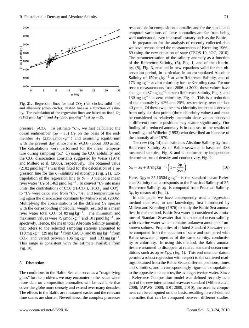
R. Feistel et al.: Density and Absolute Salinity 21

1000

1200

1400

1600

1800

2000

2200

2400

0 5 10 15 20 25 30 35

salinity

CT, A

T [

µmol

kg-

1 ]

Fig. 21: Regression lines for total CO2 (full circles, solid line) and alkalinity (open circles, dashed line) as a function of salinity. The calculation of the regression lines are based on fixed CT (2182 µmol kg-1) and AT (2350 µmol kg-1) at SP = 35.

5. Discussion The conditions in the Baltic Sea can serve as a “magnifying glass” for the problems we may encounter in the ocean when more data on composition anomalies will be available that cover the globe more densely and extend over many decades. The effects in the Baltic are measured easier and the relevant time scales are shorter. Nevertheless, the complex processes responsible for composition anomalies and for the spatial and temporal variations of these anomalies are far from being well understood, even in a small estuary such as the Baltic. In preparation for the analysis of recently collected data we have reconsidered the measurements of Kremling 1966-69 using the new equation of state (TEOS-10, IOC, 2010). The parameterisation of the salinity anomaly as a function of the Reference Salinity, (5), Fig. 1, and of the chlorinity, (8), Fig. 3, resulted in new equations valid for that observation period, in particular, in an extrapolated Absolute Salinity of 150 mg kg–1 at zero Reference Salinity, and of 173 mg kg–1 at zero chlorinity for the Kremling data. For our recent measurements from 2006 to 2009, these values have changed to 87 mg kg–1 at zero Reference Salinity, Fig. 8, and 130 mg kg–1 at zero chlorinity, Fig. 9. This is a reduction of the anomaly by 42% and 25%, respectively, over the last 40 years. Of these two, the new chlorinity intercept is derived from only six data points (three chlorinity values) and must be considered as relatively uncertain since values observed at different times or positions may scatter significantly. Our finding of a reduced anomaly is in contrast to the results of Kremling and Wilhelm (1993) who described an increase of the anomaly after 1970.

Fig. 21. Regression lines for total CO2 (full circles, solid line)and alkalinity (open circles, dashed line) as a function of salin-ity. The calculation of the regression lines are based on fixedCT(2182 µmol kg−1) andAT (2350 µmol kg−1) atSP= 35.

pressure,pCO2. To estimate◦CT, we first calculated theocean endmember (SP = 35) CT on the basis of the end-memberAT (2350 µmol kg−1) and assuming equilibriumwith the present day atmosphericpCO2 (about 380 µatm).The calculations were performed for the mean tempera-ture during sampling (5.7◦C) using the CO2 solubility andthe CO2 dissociation constants suggested by Weiss (1974)and Millero et al. (2006), respectively. The obtained value(2182 µmol kg−1) was then fixed for the calculation of a re-gression line for theCT/salinity relationship (Fig. 21). Ex-trapolation of the regression line toSP = 0 yielded a meanriver water◦CT of 1462 µmol kg−1. To convert◦CT into massunits, the contributions of CO2 (H2CO3), HCO−

3 and CO2−

3to ◦CT were calculated from◦CT, ◦AT and temperature us-ing again the dissociation constants by Millero et al. (2006).Multiplying the concentrations of the differentCT specieswith the corresponding molecular weight resulted in a meanriver water total CO2 of 89 mg kg−1. The minimum andmaximum values were 79 µmol kg−1 and 101 µmol kg−1, re-spectively. Hence, the mean total Absolute Salinity anomalythat refers to the selected sampling stations amounted to118 mg kg−1 (29 mg kg−1 from CaCO3 and 89 mg kg−1 fromCO2) and varied between 106 mg kg−1 and 133 mg kg−1.This range is consistent with the estimate available fromFig. 10.

5 Discussion

The conditions in the Baltic Sea can serve as a “magnifyingglass” for the problems we may encounter in the ocean whenmore data on composition anomalies will be available thatcover the globe more densely and extend over many decades.The effects in the Baltic are measured easier and the relevanttime scales are shorter. Nevertheless, the complex processes

responsible for composition anomalies and for the spatial andtemporal variations of these anomalies are far from beingwell understood, even in a small estuary such as the Baltic.

In preparation for the analysis of recently collected datawe have reconsidered the measurements of Kremling 1966–69 using the new equation of state (TEOS-10, IOC, 2010).The parameterisation of the salinity anomaly as a functionof the Reference Salinity, (5), Fig. 1, and of the chlorin-ity, (8), Fig. 3, resulted in new equations valid for that ob-servation period, in particular, in an extrapolated AbsoluteSalinity of 150 mg kg−1 at zero Reference Salinity, and of173 mg kg−1 at zero chlorinity for the Kremling data. For ourrecent measurements from 2006 to 2009, these values havechanged to 87 mg kg−1 at zero Reference Salinity, Fig. 8, and130 mg kg−1 at zero chlorinity, Fig. 9. This is a reductionof the anomaly by 42% and 25%, respectively, over the last40 years. Of these two, the new chlorinity intercept is derivedfrom only six data points (three chlorinity values) and mustbe considered as relatively uncertain since values observedat different times or positions may scatter significantly. Ourfinding of a reduced anomaly is in contrast to the results ofKremling and Wilhelm (1993) who described an increase ofthe anomaly after 1970.

The new (Eq. 14) that estimates Absolute SalinitySA fromReference SalinitySR of Baltic seawater is based on 436measured samples, Fig. 8, and is confirmed by independentdeterminations of density and conductivity, Fig. 9:

SA = SR+87mgkg−1·

(1−

SR

SSO

)(16)

Here, SSO = 35.16504 g kg−1 is the standard-ocean Refer-ence Salinity that corresponds to the Practical Salinity of 35.Reference Salinity,SR, is computed from Practical Salinity,SP, by means of (Eq. 2).

In this paper we have consequently used a regressionmethod that was, to our knowledge, first introduced byMillero and Kremling (1976) to study the Baltic Sea anoma-lies. In this method, Baltic Sea water is considered as a mix-ture of Standard Seawater that has standard-ocean salinity,with riverine water which contains unknown amounts of un-known solutes. Properties of diluted Standard Seawater canbe computed from the equation of state and compared withBaltic seawater properties of the same salinity, conductiv-ity or chlorinity. In using this method, the Baltic anoma-lies are assumed to disappear at related standard-ocean con-ditions such asSR = SSO, (Eq. 1). This end member datumpermits a robust regression with respect to the scattered read-ings obtained from the Baltic Sea at different positions, timesand salinities, and a correspondingly rigorous extrapolationto the opposite end member, the average riverine water. Sincea Reference Composition model was defined recently as apart of the new international seawater standard (Millero et al.,2008; IAPWS, 2008; IOC 2009, 2010), the oceanic compo-nent can be computed on this basis, resulting in well-definedanomalies that can be compared between different studies.

www.ocean-sci.net/6/3/2010/ Ocean Sci., 6, 3–24, 2010

22 R. Feistel et al.: Density and Absolute Salinity

This is a significant advantage over the earlier situation whenevery author used his particular preferred seawater composi-tion model, thus giving incompatible quantitative results forthe anomalies between different studies. Such a lack of com-parability is especially inconvenient and possibly misleadingfor trend analyses of e.g. the density anomaly on decadal orcentury time scales. We have applied this regression methodbased on the Reference Composition to the anomalies of den-sity, as described in the previous paragraph, to historical andto our recent data, as well as to the conductivity, Fig. 4, andthe sulphate anomaly, Fig. 20.

Except for the fact that the composition anomaly of theBaltic Sea is caused by the freshwater composition and isassumed to be proportional to the particular freshwater frac-tion, the method applied here does not rely on any particularproperty of the freshwater part, neither its origin nor its com-position, its variability or its age. The majority of the fresh-water in the Baltic is from river discharge, so we used “riverwater” synonymously with freshwater. The residence timeof 10–30 years implies that the largest fraction of freshwa-ter found in a given sample is not “fresh”, i.e. immediatelydischarged from a river, rather, it is aged in different waterbodies over years or decades. From the data scatter of thecorrelations it is evident that the properties of the freshwa-ter fraction are not independent of its age, its history or itsorigin. In this sense, the freshwater aging process also in-cludes sinks, sources or interactions with the sediments andthe atmosphere. We did not intend to resolve the complexprocesses that are responsible in detail for the scatter ob-served, except for the simple conservative mixing with stan-dard ocean water.

The effect of composition anomalies on the conductivity,i.e., the Practical Salinity, is considered in quantitative de-tail in recent papers of Pawlowicz (2008, 2009). The effectof such anomalies on thermodynamic properties was stud-ied by Millero (1974) by using Young’s rule. A new ap-proach to this problem is possible by Pitzer models (Feis-tel and Marion, 2007). The measurements analysed in thispaper are intended to support future model studies, first, ofthe effect of CaCO3 excess on thermodynamic properties ofseawater derived from Pitzer equations (Feistel and Marion,2007), and second, of the anomalous effects on the electri-cal conductivity of mixed aqueous electrolytes (Pawlowicz,2008, 2009). In order to support independent investigationsand future comparisons, observational data of this study areavailable from the digital Supplement (http://www.ocean-sci.net/6/3/2010/os-6-3-2010-supplement.zip) of this paper.

Since 1902, oceanographers routinely measure the salin-ity of seawater relative to certified samples of Standard Sea-water. These salinity measurements are not traceable toSI standards (Seitz, 2008) which implies reduced compa-rability and increasing uncertainty of the results on clima-tological timescales. For selected Baltic Sea samples, SI-traceable state-of-the-art measurements of electrolytic con-ductivity and density were carried out at the PTB Braun-

schweig. The results reported in Sect. 4.2 and 4.3 indi-cate that the density of seawater can be measured with sig-nificantly smaller uncertainty than the conductivity. Thesefindings support the intended proposal of the SCOR/IAPSOWG127 to calibrate instruments for salinity measurementsin the future with respect to density rather than or in additionto conductivity. Further studies are required to develop thistechnology in more detail.

Acknowledgements.The authors like to thank the crew of r/vAranda for providing seawater samples from its cruise in 2009,and Javid Safarov and the chiefmate, Mr. Langner, for provid-ing samples from the ferry “Finlandia”. They are grateful toK. Kremling and F. J. Millero for information regarding theirearlier work, and the anonymous referees for helpful hints. Thispaper contributes to the tasks of the SCOR/IAPSO Working Group127 on Thermodynamics and Equation of State of Seawater.

Edited by: R. Tailleux

References

Anderko, A. and Lencka, M. M.: Computation of electrical conduc-tivity of multicomponent aqueous systems in wide concentrationand temperature ranges, Ind. Eng. Chem. Res., 36, 1932–1943,1997.

Brinkmann, F., Dam, N. E., Deak, E., Durbiano, F., Ferrara, E.,Fuko, J., Jensen, H. D., Mariassy, M., Shreiner, R. H., Spitzer,P., Sudmeier, U., Surdu, M., and Vyskocil, L.: Primary methodsfor the measurement of electrolytic conductivity, Accred. Qual.Assur., 8, 346–353, 2003.

Comeau, S., Gorsky, G., Jeffree, R., Teyssie, J.-L., and Gattuso, J.-P.: Impact of ocean acidification on a key Arctic pelagic mollusc(Limacina helicina), Biogeosciences, 6, 1877–1882, 2009,http://www.biogeosciences.net/6/1877/2009/.

Culkin, F. and Cox, R. A.: Sodium, potassium, magnesium, calciumand strontium in seawater, Deep-Sea Res., 13, 789–804, 1966.

Culkin, F. and Smith, N.: Determination of the concentrationof potassium chloride solution having the same electrical con-ductivity, at 15◦C and infinite frequency, as standard seawaterof salinity 35.0000‰(Chlorinity 19.37394‰), IEEE J. OceanicEng., 5, 22–23, 1980.

Dickson, A. G., Sabine, C. L. and Christian, J. R.: Guide to bestpractice for ocean CO2 measurements, PICES Special Publica-tion 3, 191 pp., 2007.

Dyrssen, D.: The Baltic-Kattegat-Skagerrak estuarine system, Es-tuaries, 16, 446–452, 1993.

Feistel, R.: New shoreline map-drawing data available, Eos,80, 249, 1999, available athttp://www.io-warnemuende.de/rainer-feistel.html, 1999.

Feistel, R.: A Gibbs Function for Seawater Thermodynamics for -6 to 80◦C and Salinity up to 120 g/kg, Deep-Sea Res. Pt. I, 55,1639–1671, 2008.

Feistel, R., Feistel, S., Nausch, G., Szaron, J., Lysiak-Pastuszak, E.,and Ærtebjerg, G.: BALTIC: Monthly time series 1900–2005,edited by: Feistel, R., Nausch, G., and Wasmund, N., State andEvolution of the Baltic Sea, 1952–2005, A Detailed 50-Year Sur-vey of Meteorology and Climate, Physics, Chemistry, Biology,

Ocean Sci., 6, 3–24, 2010 www.ocean-sci.net/6/3/2010/

R. Feistel et al.: Density and Absolute Salinity 23

and Marine Environment, John Wiley & Sons, Inc., Hoboken,311–336, 2008.

Feistel, R. and Marion, G. M.: A Gibbs-Pitzer Function for High-Salinity Seawater Thermodynamics, Progr. Oceanogr., 74, 515–539, 2007.

Feistel, R. and Weinreben, S.: Is Practical Salinity conserva-tive in the Baltic Sea? available at:http://www.iopan.gda.pl/oceanologia/501.html#A6, Oceanologia, 50, 73–82, 2008.

Feistel, R., Wright, D. G., Jackett, D. R., Miyagawa, K., Reissmann,J. H., Wagner, W., Overhoff, U., Guder, C., Feistel, A., and Mar-ion, G. M.: Numerical Implementation and Oceanographic Ap-plication of the Thermodynamic Potentials of Water, Vapour, Ice,Seawater and Air. Part I: Background and Equations, Ocean Sci-ence, submitted, 2010.

Fonselius, S. H.: Hydrography of the Baltic deep basins II, FisheryBoard of Sweden, Ser. Hydrogr., 20, 1–31, 1967.

Forch, C., Knudsen, M. and Sørensen, S. P. L.: Berichteuberdie Konstantenbestimmungen zur Aufstellung der hydrographis-chen Tabellen, gesammelt von Martin Knudsen, Det KongeligeDanske Videnskabernes Selskabs Skrifter, 6, 1–152, 1902.

GUM: Evaluation of measurement data – Guide to the expression ofuncertainty in measurement (GUM), JCGM 100:2008, availableatwww.bipm.org/en/publications/guides/gum, 2008.

Hjalmarsson, S., Wesslander, K., Anderson, L. G., Omstedt, A.,Perttila, M., and Mintrop, L.: Distribution, long-term develop-ment and mass balance calculation of total alkalinity in the BalticSea, Cont. Shelf Res., 28, 593–601, 2008.

IAPWS: Release on the IAPWS Formulation 2008 for the Thermo-dynamic Properties of Seawater, The International Associationfor the Properties of Water and Steam, Berlin, Germany, Septem-ber 2008, available at:http://www.iapws.org, 2008.

IOC: Resolution XXV-7, INTERNATIONAL THERMODY-NAMIC EQUATION OF SEAWATER (TEOS-10), INTER-GOVERNMENTAL OCEANOGRAPHIC COMMISSION (ofUNESCO), Twenty-fifth Session of the Assembly, Paris, 16–25 June 2009.

IOC, 2010: The international thermodynamic equation of seawa-ter – Calculation and use of thermodynamic properties, Inter-governmental Oceanographic Commission, Manuals and GuidesNo. xx., UNESCO (English), 171 pp., available athttp://www.TEOS-10.org, 2010.

Jones, N.: Metrology: The new and improved kelvin, Nature, 459,902–904, 2009.

Knudsen, M.: Hydrographische Tabellen, G. E. C. Gad, Copen-hagen, 1901.

Kremling, K.: Untersuchungen zur chemischen Zusammensetzungdes Meerwassers aus der Ostsee I, Kiel. Meeresforsch., 25, 81–104, 1969.

Kremling, K.: Untersuchungen zur chemischen Zusammensetzungdes Meerwassers aus der Ostsee II, Kiel. Meeresforsch., 26, 1–20, 1970.

Kremling, K.: New method for measuring density of seawater, Na-ture, 229, 109–110, 1971.

Kremling, K.: Untersuchungen zur chemischen Zusammensetzungdes Meerwassers aus der Ostsee III, Kiel. Meeresforsch., 28, 99–118, 1972.

Kremling, K. and Wilhelm, G.: Recent increase of the calcium con-centrations in Baltic Sea waters, Mar. Poll. Bull., 34, 763–767,1997.

Kwiecinski, B.: The relation between the chlorinity and the con-ductivity in Baltic water, Deep-Sea Res., 12, 113–120, 1965.

Marion, G. M., Millero, F. J., and Feistel, R.: Precipitation of solidphase calcium carbonates and their effect on application of sea-waterSA–T –P models, Ocean Sci., 5, 285–291, 2009,http://www.ocean-sci.net/5/285/2009/.

Matthaus, W., Nehring, D., Feistel, R., Nausch, G., Mohrholz, V.,and Lass, H. U.: The inflow of highly saline water into the BalticSea, edited by: Feistel, R., Nausch, G., and Wasmund, N., Stateand Evolution of the Baltic Sea, 1952–2005, A Detailed 50-YearSurvey of Meteorology and Climate, Physics, Chemistry, Biol-ogy, and Marine Environment, John Wiley & Sons, Inc., Hobo-ken, 265–309, 2008.

McDougall, T. J., Jackett, D. R., and Millero, F. J.: An algorithmfor estimating Absolute Salinity in the global ocean, Ocean Sci.Discuss., 6, 215–242, 2009,http://www.ocean-sci-discuss.net/6/215/2009/.

Meier, H. E. M.: Modeling the pathways and ages of inflowing salt-and freshwater in the Baltic Sea estuarine, Coast. Shelf Sci., 74,610–627, 2007.

Meier, H. E. M., Feistel, R., Piechura, J., Arneborg, L., Burchard,H., Fiekas, V., Golenko, N., Kuzmina, N., Mohrholz, V., Nohr,C., Paka, V. T., Sellschopp, J., Stips, A., and Zhurbas, V.: Ven-tilation of the Baltic Sea deep water: A brief review of presentknowledge from observations and models, Oceanologia, 48(S),133–164, available athttp://www.iopan.gda.pl/oceanologia/48S.html#A8, 2006.

Millero, F. J.: Seawater as a multicomponent electrolyte solution,The Sea, edited by: Goldberg, E. D., Wiley-Interscience, 5, 3–80, 1974.

Millero, F. J.: The marine inorganic carbon cycle, Chem. Rev., 107,308–341, 2007.

Millero, F. J., Feistel, R., Wright, D. G. and McDougall, T. J.:The composition of Standard Seawater and the definition of theReference-Composition Salinity Scale, Deep-Sea Res. Pt. I, 55,50–72, 2008.

Millero, F. J., Forsht, D., Means, D., Giekes, J., and Kenyon, K.:The density of North Pacific Ocean waters. J. Geophys. Res. 83,2359–2364, 1978.

Millero, F. J., Graham, T. B., Huang, F., Bustos-Serrano, H., andPierrot, D.: Dissociation constants of carbonic acid in seawateras a function of salinity and temperature, Mar. Chem., 100, 80–94, 2006.

Millero, F. J., Huang, F., Williams, N., Waters, J., and Woosley, R.:The effect of composition on the density of South Pacific Oceanwaters, Mar. Chem. 114, 56–62, 2009.

Millero, F. J. and Kremling, K.: The densities of Baltic Waters,Deep-Sea Res., 23, 1129–1138, 1976.

Millero, F. J, Waters, J., Woosley, R., Fen Huang, F., and MarevaChanson, M.: The effect of composition on the density of IndianOcean waters, Deep-Sea Res. Pt. I, 55, 460–470, 2008.

Morris, A. W. and Riley, J. P.: The bromide/chlorinity and sul-phate/chlorinity ratio in seawater, Deep-Sea Res., 13, 699–705,1966.

Nausch, G., Nehring, D., and Nagel, K.: Nutrient concentrations,trends and their relation to eutrophication, edited by: Feistel, R.,Nausch, G., and Wasmund, N., State and Evolution of the BalticSea, 1952–2005, A Detailed 50-Year Survey of Meteorology andClimate, Physics, Chemistry, Biology, and Marine Environment,

www.ocean-sci.net/6/3/2010/ Ocean Sci., 6, 3–24, 2010

24 R. Feistel et al.: Density and Absolute Salinity

John Wiley & Sons, Inc., Hoboken, 265–309, 2008.Nehring, D.: Das Nahrstoffregime der Ostsee – seine

Veranderungen im Zeitraum 1969 bis 1978 – Ursachenund Auswirkungen, Dissertation B, Warnemunde 1980.

Nehring, D. and Rohde, K.-H.: Weitere Untersuchungenuberanomale Ionenverhaltnisse in der Ostsee, Beitr. Meeresk., 20,10–33, 1967.

Nessim, R. B. and Schlungbaum, G.: Untersuchungen zur Salzge-haltsanomalie, Wiss. Z. Wilhelm-Pieck-Univ. Rostock, 29,No. 3/4, 1980.

Ohlson, M. and Anderson, L.: Recent investigation of total carbon-ate in the Baltic Sea: changes from the past as a result of acidrain? Mar. Chem., 30, 259–267, 1990.

Omstedt, A., Gustafsson, E., and Wesslander, K.: Modelling theuptake and release of carbon dioxide in the Baltic Sea surfacewater, Cont. Shelf Res., 29, 870–885, 2009.

Pawlowicz, R.: Calculating the conductivity of natural waters, Lim-nol. Oceanogr.-Methods, 6, 489–501, 2008.

Pawlowicz, R.: A model for predicting changes in the electricalconductivity, practical salinity, and absolute salinity of seawaterdue to variations in relative chemical composition, Ocean Sci.Discuss., 6, 2861–2909, 2009,http://www.ocean-sci-discuss.net/6/2861/2009/.

Perkin, R. G. and Lewis, E. L.: The Practical Salinity Scale 1978,Fitting the data, IEEE J. Ocean. Eng., OE-5, 9–16, 1980.

Reissmann, J. H., Burchard, H., Feistel, R., Hagen, E., Lass, H.U., Mohrholz, V., Nausch, G., Umlauf, L., and Wieczorek, G.:State-of-the-art review on vertical mixing in the Baltic Sea andconsequences for eutrophication, Progr. Oceanogr., 82, 47–80,2009.

Rohde, K.-H.: Untersuchungenuber die Calcium- und Magnesiu-manomalie in der Ostsee, Beitr. Meeresk., 19, 18–31, 1966.

SeaBird: 1978 Practical Salinity Scale, Application Note No. 14,revised January 1989, last modified 6 July 2009, Sea-Bird Elec-tronics, available at:http://www.seabird.com/applicationnotes/AN14.htm, 1989.

Seitz, S., Spitzer, P., and Brown, R. J. C.: Consistency of practi-cal salinity measurements traceable to primary conductivity stan-dards: Euromet project 918, Accred. Qual. Assur., 13, 601–605,2008.

Stalcup, M. C.: Salinity Measurements, WOCE Operations Manual,Part 3.1.3, WHP Operations and Methods, 1991.

Stigebrandt, A. and Wulff, F.: A time-dependent budget model fornutrients in the Baltic Sea, Glob. Biochem. Cy., 3, 63–78, 1989.

Thomas, H. and Schneider, B.: The seasonal cycle of carbon diox-ide in Baltic Sea surface waters, J. Mar. Sys., 22, 53–67, 1999.

Trzosinska, A.: Metoda Knudsena-Sorensen w zastosowaniu dobedania zasolenia wody potudniowego Baltiku, Przegl. Geofiz.,314, 84–88, 1967.

Veron, J. E. N., Hoegh-Guldberg, O., Lenton, T. M., Lough, J. M.,Obura, D. O., Pearce-Kelly, P., Sheppard, C. R. C., Spalding, M.,Stafford-Smith, M. G., and Rogers, A. D.: The coral reef crisis:The critical importance of< 350 ppm CO2, Mar. Poll. Bull. 58,1428–1436, 2009.

VIM: International vocabulary of metrology - Basic and generalconcepts and associated terms (VIM), JCGM 200:2008, avail-able atwww.bipm.org/en/publications/guides/vim, 2008.

Voipio, A.: On the magnesium content in the Baltic, SuomenKemistilehti, B30, 84–88, 1957.

Weiss, R. F.: Carbon dioxide in water and seawater: the solubilityof a non-ideal gas, Mar. Chem., 2, 203–215, 1974.

Wolf, H.: Determination of water density: limitations at the un-certainty level of 1×10−6, Accred. Qual. Assur., 13, 587–591,2008.

Wright, D. G., Feistel, R., Jackett, D. R., Miyagawa, K., Reissmann,J. H., Wagner, W., Overhoff, U., Guder, C., Feistel, A., and Mar-ion, G. M.: Numerical Implementation and Oceanographic Ap-plication of the Thermodynamic Potentials of Water, Vapour, Ice,Seawater and Air. Part II: The Library Routines, Ocean Science,to be submitted, 2010.

Zarins, E. and Ozolins, J.: Untersuchungenuber die Zusammenset-zung des Meerwassers im Rigaischen Meerbusen und an der lett-landischen Kuste des baltischen Meeres, J. Conseil, 10, 275–301,1935.

Ocean Sci., 6, 3–24, 2010 www.ocean-sci.net/6/3/2010/