Temperature Effect on the Soil Water Retention Characteristic

By

Maie El-Keshky

A Thesis Presented in Partial Fulfillment of the Requirements for the Degree

Master of Science

Approved July 2011 by the Graduate Supervisory Committee:

Claudia Zapata, Chair Edward Kavazanjian

Sandra Houston

ARIZONA STATE UNIVERSITY

August 2011

i

ABSTRACT

The importance of unsaturated soil behavior stems from the fact that a

vast majority of infrastructures are founded on unsaturated soils.

Research has recently been concentrated on unsaturated soil properties.

In the evaluation of unsaturated soils, researchers agree that soil water

retention characterized by the soil water characteristic curve (SWCC) is

among the most important factors when assessing fluid flow, volume

change and shear strength for these soils.

The temperature influence on soil moisture flow is a major concern in the

design of important engineering systems such as barriers in underground

repositories for radioactive waste disposal, ground-source heat pump

(GSHP) systems, evapotranspirative (ET) covers and pavement systems..

Accurate modeling of the temperature effect on the SWCC may lead to

reduction in design costs, simpler constructability, and hence, more

sustainable structures.

. The study made use of two possible approaches to assess the

temperature effect on the SWCC. In the first approach, soils were sorted

from a large soil database into families of similar properties but located on

sites with different MAAT. The SWCCs were plotted for each family of

soils. Most families of soils showed a clear trend indicating the influence of

temperature on the soil water retention curve at low degrees of saturation..

The second approach made use of statistical analysis. It was

demonstrated that the suction increases as the MAAT decreases. The

ii

statistical analysis showed that even though the plasticity index proved to

have the greatest influence on suction, the mean annual air temperature

effect proved not to be negligible. In both approaches, a strong

relationship between temperature, suction and soil properties was

observed. Finally, a comparison of the model based on the mean annual

air temperature environmental factor was compared to another model that

makes use of the Thornthwaite Moisture Index (TMI) to estimate the

environmental effects on the suction of unsaturated soils. Results showed

that the MAAT can be a better indicator when compared to the TMI found

but the results were inconclusive due to the lack of TMI data available.

iii

DEDICATION

To my husband and kids

iv

ACKNOWLEDGMENTS

I am truly indebted to the advice and guidance of Dr. Claudia Zapata

committee chairman. Thank you, Dr. Claudia, for your teaching, support,

patience and assistance during my time at ASU.

I would like to thank Dr. Edward Kavazanjian for being part of my

committee.

Acknowledgements are given to Dr. Sandra Houston who has given me so

many ideas during teaching the course on unsaturated soil mechanics,

and for being part of my committee.

I would like to especially thank my husband Eslam so much for all his

support, patience, encouragements, and for his faith in me. Finally, I would

like to thank my son Yaseen and my daughter Malak for all their love and

patience.

v

TABLE OF CONTENTS

LIST OF TABLES ......................................................................................... vi

LIST OF FIGURES ........................................................................................ x

CHAPTER

1 Chapter 1........................................................................................ 1

OVERVIEW ....................................................................................... 1

Thesis objectives ..................................................................... 2

Thesis organization ................................................................. 3

Chapter 2........................................................................................... 5

LITERATURE REVIEW .................................................................... 5

Soil water retention characteristic of unsaturated soil ............. 5

The importance of the SWCC in different fields ...................... 9

Methods to measure the soil suction ..................................... 11

Filter paper ..................................................................... 11

Psychrometers ............................................................... 11

Tensiometer ................................................................... 12

Pressure plate and pressure membrane ........................ 13

Soil water retention curve determined by gamma-ray

beam attenuation ........................................................... 13

Measurement of soil-water characteristic curves for fine-

grained soils using a small-scale centrifuge ................... 15

vi

The importance of the temperature effect on the soil water

retention ................................................................................. 16

Chapter 3......................................................................................... 18

SUCTION TEMPERATURE DEPENDENCE MODELS ................. 18

Theories explaining the temperature effects on soil water

retention ................................................................................. 18

Models available to estimate moisture flow under the effect of

temperature in unsaturated soils ........................................... 22

Non-isothermal models .................................................. 22

Another theory explaining the effect of temperature on the

retention curves proposed by (W. Wu et al., 2004) ........ 23

Previous studies on the effect of temperature on the SWCC

and their limitations ................................................................ 25

Models available for the temperature effect on the

hydraulic conductivity ..................................................... 26

Effect of temperature on hydraulic conductivity .............. 28

Chapter 4......................................................................................... 30

ANALYSIS AND VALIDATION OF EXISTING MODELS ............... 30

Database selection and processing ...................................... 30

Properties available for each soil unit .................................... 31

Temperature effect evaluation ....................................... 31

Results and analysis .............................................................. 34

vii

Comparison with Grant model for temperature effect on

suction ................................................................................... 36

Assessment of the accuracy of the βo parameter ................. 38

Summary and conclusions .................................................... 42

Chapter 5......................................................................................... 44

STATISTICAL ANALYSIS MODEL................................................. 44

Sample soil selection and procedure ............................. 44

Statistical analysis and results ....................................... 45

Suction-PI sensitivity analysis ........................................ 47

Suction_Passing200 Sensitivity Analysis ....................... 48

Summary and conclusion ............................................... 49

Chapter 6......................................................................................... 50

STATISTICAL ANALYSIS MODEL USING TMI ............................. 50

Minitab Analysis ..................................................................... 52

Regression Analysis: Suction versus Passing 200, PI, and

TMI ......................................................................................... 52

Summary and conclusion ............................................... 53

Chapter 7......................................................................................... 54

CONCLUSION AND RECOMMENDATION FOR FUTURE WORK

............................................................................................. 54

Conclusion with respect to the Grant equation ..................... 54

viii

Conclusion with respect to statistical model to incorporate the

temperature effect on suction ................................................ 55

Conclusion with respect to statistical model to incorporate the

TMI effect on suction ............................................................. 56

Recommendation for future work .......................................... 56

REFERENCES ......................................................................................... 58

APPENDIX

A SWCC PLOTS FOR SOIL GROUPS WITH SAME

CHARACTARISTICS AT DIFFERENT TEMPS ................. 63

ix

LIST OF TABLES

Table Page

1. Comparison between existing and calculated equations ...................... 48

2. βo values ............................................................................................... 50

x

LIST OF FIGURES

Figure Page

Figure 1 Soil water characteristic curves (Fredlund and Xing 1994) .......... 6

Figure 2 Hysteresis, desorption and adsorption curves (Vanapalli and

Fredlund 1996) .......................................................................................... 7

Figure 3 Scheme of the gamma-ray beam attenuation system to valuate

soil water retention curves (Williams et al. 1992)..................................... 14

Figure 4 Small-scale centrifuge ............................................................... 16

Figure 5 Temperature dependence of physicochemical properties of water

(Grifoll 2005) ............................................................................................ 17

Figure 6 A family with Passing200=80 and PI= 23.5 ............................... 32

Figure 7 A family with Passing200=80 and PI= 39.5 ............................... 32

Figure 8 Mean annual air temperature map (NOAA) ............................... 33

Figure 9 SWCCs for Passing 200=60 and PI=7.5 .................................. 34

Figure 10 Relation between temperature and suction for soils with passing

200=60 .................................................................................................... 35

Figure 11 Difference between 0β values calculated from the analysis and

calculated from existing model ................................................................ 38

Figure 12 Soils distribution map used in the statistical analysis .............. 45

Figure 13 Minitab(R) regression analysis output ..................................... 46

Figure 14 Proposed Bo value .................................................................. 47

Figure 15 Effect of temperature on suction for different PI values ........... 48

xi

Figure 16 Effect of temperature on suction with different passing 200 .... 49

Figure 17 Thornthwaite Moisture Index Contour Map .............................. 50

Figure 18 Regression analysis for TMI versus suction ............................ 53

1

Chapter 1

OVERVIEW

There are a variety of important geotechnical problems where temperature

variation occurs during water flow in unsaturated soils. Examples of

where this thermo-hydraulic phenomenon is important include: 1) Thermal

behavior of ground as a source of geothermal energy; 2) Analysis of

barriers for nuclear waste storage; 3) Water balance of evapotranspirative

(ET) covers for municipal solid waste containment; 4) Assessment of

vapor barriers for building slabs and subsurface walls; 5) Heat

transfer/dissipation from buried electrical cables, underground tanks and

pipelines; 6) Heat applied directly to the soil to clean up degraded areas;

7) Vapor migration calculations at contaminated soil and groundwater

sites, and remediation performance estimates; and 8) Coupled thermal-

moisture movements in pavement systems. During these thermo-hydraulic

processes, temperature variation near the potential site can give rise to

both water vaporization in the high temperature zone, and condensation in

the low temperature zone. Other typical examples involving temperature

effects on unsaturated flow include, steam flushing for removal of non-

aqueous phase fluids from the subsurface (She and Sleep 1998).

Understanding and modeling this process is critical for assessing the

engineering design for each application.

2

It has been agreed upon that hydraulic properties of porous media such as

hydraulic conductivity and water retention are temperature-dependent. Not

taking this properties effect into account can cause an error in the design

process (Philip and de Vries 1957).

There has been a substantial amount of effort in understanding the

temperature effect on the hydraulic conductivity by using the viscosity

theory (Hopmans and Dane 1986). However, there has been a minimal

effort in explaining the temperature effect on the soil water characteristic

curve. Most of the previous experimental and theoretical efforts have been

restricted to clay soil or bentonite. Moreover, a study that considers a wide

variety of soils or a wide range of temperatures could not be found

(Jacinto et al. 2007).

Thesis objectives

In this study, soil properties and information of a wide range of soils were

collected from a large database available from the National Resources

Conservation Service. The main objective of this thesis work was to

assess the effect of temperature on the soil water characteristic curve.

The objective of this study was accomplished by following two different

approaches. The first approach consisted of validating the equation

proposed by Grant in 2005. This equation models the effect of

temperature on soil suction. The second approach made use of statistical

analysis in order to quantify the effect of the mean annual air temperature

3

on suction, by analyzing data for more than 4,800 soils at different

locations in the United States.

Thesis organization

Chapter 1 provides a brief introduction, including the thesis objectives and

document organization.

Chapter 2 presents a detailed literature review including a description of

the soil water characteristic curve, methods and equipment to measure

suction, and its importance and applications. Chapter 2 also includes a

brief summary on the importance of temperature effect on soil water

retention.

Chapter 3 covers the existing proven models that relate soil suction and

temperature; while Chapter 4 includes an assessment of the suction

dependence on temperature described by the equation proposed by Grant

in 2005 based on the van Genuchten SWCC equation. This analysis is

based on the SWCC of soils with similar characteristics at different

temperature zones.

Chapter 5 covers the statistical analysis of the temperature effect on

suction for a sample of 4,800 soils at different temperature zones in the

United States. A proposed simple model that includes the mean annual

air temperature (MAAT) and soil properties is presented in this chapter.

4

Chapter 6 presents an attempt to assess the effect of the combined

environmental effects represented by the Thornthwaite Moisture Index

(TMI) on soil suction by utilizing statistical analysis.

Finally, Chapter 7 presents the conclusions with a brief summary of the

results. Topics for future research related to the work accomplished and

presented in this thesis are also presented.

5

Chapter 2

LITERATURE REVIEW

Soil water retention characteristic of unsaturated soil The soil-water characteristic curve illustrates the relationship of soil matric

suction (ua-uw) and gravimetric water content w, or the volumetric water

content θ, or the degree of Saturation Sr, and it is a measure of the water

storage capacity of the soil for a given matric suction. The air entry value

and high residual suction level can be derived from the SWCC. The shear

strength, hydraulic conductivity, permeability function, chemical diffusivity,

water storage, unfrozen volumetric water content, specific heat, and

thermal conductivity are all functions of the SWCC. There are several

devices to determine the SWCC in the lab and in field, such as; the

suction plate, the pressure plate, filter paper, psychrometers, tensiometer,

and gamma-ray beam attenuation. Some of these methods are used to

measure the matric suction while others are used to measure the total

suction.

SWCC is normally plotted on a semi-logarithmic scale for the suction

range used in geotechnical practice. Figure 1 shows a schematic

representation of the different components of the SWCC function.

6

Figure 1 Soil water characteristic curves (Fredlund and Xing 1994)

The air entry value or bubbling pressure stands for the differential

pressure between the air and water that is required to cause desaturation

of the largest pores (Vanapalli and Fredlund 1996). It is important to know

that the process of desaturation happens only at suction values greater

than the air entry value. At high suction level (above 1,500 kPa), matric

suction and the total suction can be analogous. At suction values smaller

than the air entry value, the soil is considered to be saturated. The air

entry value of the soil can be estimated by extending the constant slope

portion of the soil water characteristic curve to intersect the suction axis at

100% saturation.

There are three identifiable stages of desaturation as shown in Figure 1:

the boundary effect stage, the transition stage, and the residual stage of

7

desaturation. In the boundary effect stage, water fills all the soil pores. The

soil is saturated in this region, In the transition zone, the connectivity of the

water in the voids or pores continue to reduce with increased values of

suction, and eventually large increases in suction lead to relatively small

changes in the degree of saturation. The residual state of saturation can

be considered to be the degree of saturation at which the liquid phase

becomes discontinuous. The residual state of saturation represents the

stage beyond which it becomes increasingly difficult to remove water from

a specimen by drainage (Vanapalli and Fredlund 1996).

Figure 2 Hysteresis, desorption and adsorption curves (Vanapalli and Fredlund 1996)

The SWCC presents a hysteresis. Figure 2 illustrates this phenomenon

where hysteresis causes the desorption curve and the adsorption curve to

differ. It is believed that the entrapped air may cause the end point of the

8

adsorption curve differ from the starting point of the desorption curve. On

the other hand, the total suction corresponding to zero degree of

saturation appears to be the same for all soil types. A value slightly below

106 kPa has been experimentally supported by research done in a number

of different soils (Croney and Coleman 1961). This value is also

supported by thermodynamic considerations (Richards 1965). In other

words, there is a maximum total suction value corresponding to a zero

relative humidity in any porous medium.

As the soil plasticity increases, the air entry value and the saturated water

content increase. Therefore, for the same degree of saturation level,

plastic soils have higher suction values than non-plastic soils.

The relationship developed between degree of saturation level and suction

is based on the pore size distribution of the soil. That means that when

the pore size distribution of the soil is either predicted or obtained, then

the SWCC is uniquely determined from a general equation. Existing

equations fit experimental data reasonably well over the entire suction

range from 0 to 106 KPa.

Many equations have been proposed to represent the SWCC. Most of

these equations are empirical and are based on the shape of the SWCC.

The most common equation is the one proposed by Fredlund and Xing

(1994):

9

m

ns

ae

+

=ψ

θθln

1 ………………………………………………….[1]

Where θ is the volumetric water content, θ is a parameter closely related

to the air entry value, and n and m are fixed parameters that control the

slope of the SWCC. In general, the value of parameter θ is higher than

the air entry value and corresponds to the suction value at the inflection

point. However, for a small m value, the air entry value can be

approximated by the parameter a.

The importance of the SWCC in different fields The shape of the SWCC depends on the pore size distribution and

compressibility of the soil. These two characteristics of porous materials

are affected by the initial water content, soil structure, mineralogy, and the

stress history (Lapierre et al. 1990; Vanapalli et al. 1999; Simms and

Yanful 2000). Most SWCCs are S shaped. The curve shapes are a

response to the pore size distribution of the material. For a rigid porous

material of single pore size or uniform pore size distribution, whether it is a

soil or not, the SWCC should be similar to the curve shown in Figure 1.

However, complete water loss with suction increasing beyond the air entry

value is not usual. In other words, it is difficult to remove all the water from

a porous material by means of a small increase in suction (Fredlund and

Rahardjo 1993). A material with a great number of pore sizes should

10

present a more gradual reduction in water content with an increase in

suction.

Suction changes due to moisture flow, and seepage control the strength

and deformation behavior of unsaturated soils. Hence, accurate

characteristic of moisture flow is often critical to both stability and

deformation problems.

The expansive soil is a particular clay that is of special characteristics (i.e.,

swell–shrinking, crack and over-consolidation characteristics). The

characterization of the expansive soil is strongly related to the change in

suction. In general, the behavior of an unsaturated soil is strongly related

to the pore size and pore geometrical distribution.

SWCC behavior can be a useful tool to understand the stabilization effects

on expansive soils. A research experiment was conducted on expansive

soil using two different types of fly ash (Lapierre et al. 1990; Vanapalli et

al. 1999; Simms and Yanful 2000). The volumetric water contents of fly

ash-treated soils decreased with an increase in the percentage of fly ash

stabilizers. These changes are attributed to modifications in both particle

size and moderate cementing effects in stabilized soils. The fine fly ash

materials, similar to cement stabilizers, reduce pore void distribution of

clayey soils by occupying their voids and also bond finer clay particles at

contact points. As a result, fly ash-treated soils exhibit moderate to low

plastic soil behavior with low volumetric moisture contents.

11

Methods to measure the soil suction

Filter paper The filter paper method for total and matric suction measurements was

originated in Europe in the 1920’s and brought to the United States by

Gardner in 1937. A filter paper in contact with the soil specimen allows

water in the liquid phases and solutes to exchange freely and therefore,

matric suction is measured. A filter paper that is not in contact with the soil

specimen only permits water exchange in the vapor phase and therefore

measures the total suction (Rahardjo and Leong 2006). The filter paper

comes to equilibrium with the soil after several days in a constant

temperature environment. An upper limit of 14 days equilibrium time is

recommended although the recommendation might not be necessarily

correct for clayey materials. After equilibration, the suction value of the soil

and the filter paper is equal and the water content of the filter paper can

be measured. The corresponding suction value can be inferred by using a

filter paper wetting calibration curve developed with osmotic salt solutions.

This method is based on the thermodynamic relationship between osmotic

suction and the relative humidity.

Psychrometers

Thermocouple psychrometers can measure the soil total suction by

measuring the relative humidity in the air phase of the soil pores or the

region near the soil. The Peltier psychrometer is commonly used in geo-

technical practice. It operates on the basis of temperature difference

12

measurements between a non-evaporating surface (dry bulb) and an

evaporating surface (wet bulb). The temperature difference is related to

the relative humidity. Using Seeback effect and Peltier effect, the

thermocouple psychrometer can measure the total suction in a soil sample

by using the established calibration curve. This curve relates the microvolt

outputs from the thermocouple and a known total suction value (Tang et

al., 1997)

Tensiometer Tensiometer utilizes a high air entry ceramic cup as an interface between

the measuring system and the negative pore-water pressure in the soil.

The high air entry porous ceramic cup is connected to a pressure

measuring device through a small bore tube. The tube and the cup are

filled with de-aired water. Then the cup is inserted into a pre-cored hole

and keeps a good contact with the soil. Once equilibrium is established

between the soil and the measuring system, the water in the tensiometer

has the same negative pressures as the pore-water in the soil (Fredlund

and Rahardjo 1993b). Thus, matric suction can be measured. Unlike the

filter paper method and the axis-translation apparatus that can be only

used in the laboratory, the tensiometers can be applied both in the

laboratory and the field (Fredlund and Rahardjo 1993b).

13

Pressure plate and pressure membrane The pressure plate and the pressure membrane are typically used to

determine the matric suction (ua-uw), and the Soil-Water Characteristic

Curve (SWCC). The main difference between the pressure plate and

pressure membrane apparatus is that the pressure plate uses a ceramic

porous disk (normally having the air-entry value of 1 bar, 3 bars, 5 bars or

15 bars) while the pressure membrane uses a cellulose membrane with

an air-entry value of 15 bars. The suction equilibrium time is determined

by the observation of the variation of the water level in a burette

connected to the ceramic disk.

Soil water retention curve determined by gamma-ray beam attenuation Practical problems still remain with the pressure chamber, e.g. (1) the

difficulty of a correct judgment of equilibrium (2) the risk of changes in soil

structure and water retention characteristics of the sample due to its

frequent manipulation during measurements at each chosen potential and

(3) the long time required for the whole process, mainly due to sample

weighing and resaturation (also affected by hysteresis) after each

equilibrium (Williams et al. 1992). The gamma ray beam attenuation

method avoids the need of frequent sample manipulation as in the case of

the pressure chamber method. The water content can be continuously

monitored inside the chamber allowing a more precise judgment of the

equilibrium. The time required for the retention curve determination can be

14

significantly reduced in comparison with the traditional method. A

schematic representation of this method is shown in Figure 3. This method

is an adaptation of the conventional pressure chamber to permit the

gamma-ray beam to pass through the soil sample inside the chamber,

allowing for continuous soil moisture monitoring during the whole process

of soil water retention measurements, without the opening of the chamber

for measurements at each step. This new improvement leads also to a

more precise judgment of equilibrium, since soil moisture is continuously

monitored inside the chamber. Sample manipulation is eliminated since it

is saturated only once at the beginning of the process, minimizing the risk

of modifications in structure and, as a consequence, the time required for

the whole water retention curve establishment is shortened (Bacchi et al.

1998).

Figure 3 Scheme of the gamma-ray beam attenuation system to valuate soil water retention curves (Williams et al. 1992)

15

The nuclear method presents some advantages over the traditional

method including the higher accuracy in the determination of time of

equilibrium and the reduction in the time required for the whole retention

curve determination. This is because the soil sample in the nuclear

method is submitted only one time to the wetting and drying processes.

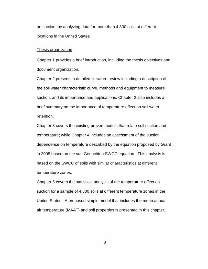
Measurement of soil-water characteristic curves for fine-grained soils using a small-scale centrifuge Commercially available small-scale centrifuges can be used to obtain

multiple water contents versus suction data points for the soil-water

characteristic curve at a single speed of rotation.

A high gravity field is applied to an initially saturated soil specimen in the

centrifuge. The soil specimen is supported on a saturated, porous ceramic

column. The base of the ceramic stone rests in a water reservoir that is at

atmospheric pressure conditions. The water content profile in the soil

specimen after attaining equilibrium is similar to water draining under in

situ conditions to a groundwater table where gravity is increased several

times.

The time period for measuring the soil-water characteristic curves for fine-

grained soils reduces considerably using the centrifuge method in

comparison to conventional testing procedures such as the pressure plate

apparatus or a pressure cell. (Khanzode et al, 2002)

16

Figure 4 Small-scale centrifuge

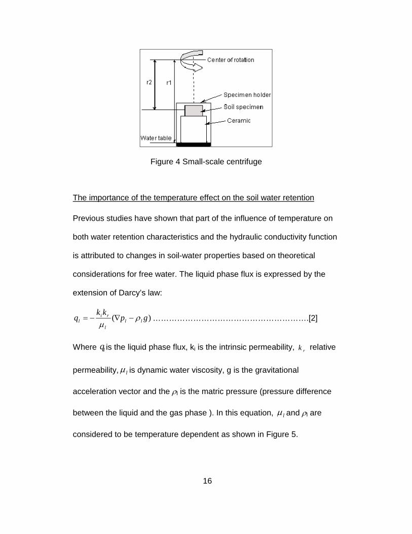
The importance of the temperature effect on the soil water retention Previous studies have shown that part of the influence of temperature on

both water retention characteristics and the hydraulic conductivity function

is attributed to changes in soil-water properties based on theoretical

considerations for free water. The liquid phase flux is expressed by the

extension of Darcy’s law:

)( gpkk

q lll

ril ρ

µ−∇−= ………………………………………………….[2]

Where lq is the liquid phase flux, ki is the intrinsic permeability, rk relative

permeability, lµ is dynamic water viscosity, g is the gravitational

acceleration vector and the ρl is the matric pressure (pressure difference

between the liquid and the gas phase ). In this equation, lµ and ρl are

considered to be temperature dependent as shown in Figure 5.

17

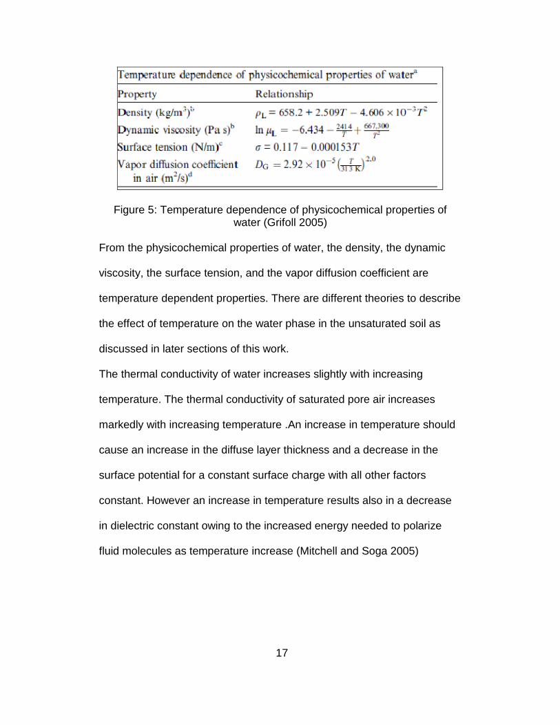
Figure 5: Temperature dependence of physicochemical properties of water (Grifoll 2005)

From the physicochemical properties of water, the density, the dynamic

viscosity, the surface tension, and the vapor diffusion coefficient are

temperature dependent properties. There are different theories to describe

the effect of temperature on the water phase in the unsaturated soil as

discussed in later sections of this work.

The thermal conductivity of water increases slightly with increasing

temperature. The thermal conductivity of saturated pore air increases

markedly with increasing temperature .An increase in temperature should

cause an increase in the diffuse layer thickness and a decrease in the

surface potential for a constant surface charge with all other factors

constant. However an increase in temperature results also in a decrease

in dielectric constant owing to the increased energy needed to polarize

fluid molecules as temperature increase (Mitchell and Soga 2005)

18

Chapter 3

SUCTION TEMPERATURE DEPENDENCE MODELS

Theories explaining the temperature effects on soil water retention Different theories have been proposed to explain the relation between

temperature and soil suction. Considering soil water composed of

continuous water and isolated packets of water, the continuous water

content change linearly with the total water content. When temperature

increases, water flows from isolated packets to the continuous water

phase. This results in a shift in the SWCC. Also there are additional

factors contributing to temperature effect on the SWCC such as entrapped

air and difference between surface tension of the soil solution and pure

water. Entrapped air may play a role in the temperature coefficient of the

soil water pressure head, which includes the effect of entrapped air.

Entrapped air volume is expected to decrease with decreasing water

content, because a large number of pores become part of the continuous

air phase.

Hopmans and Dane (1986b) measured the water retention curve

corresponding to the total entrapped air volumes and the surface tension

of the soil solution at two temperatures. The study showed that the effect

of entrapped air volume decreased the effect of temperature on the water

retention curve. The authors demonstrated that ignoring temperature

effects on soil hydraulic properties can result in substantial prediction error

in water movement (Hopmans and Dane 1985).

19

Liu and Dane proposed a theory that assumes that the soil water forms a

continuum and the isolated water packets do not contribute to soil

hydraulic equilibrium (Liu and Dane 1993). If water inside a capillary tube

is in hydraulic equilibrium, then:

gRRL

ρ

σ )2

1

1

1(2 −

= …………………………………………….……….[3]

Where σ is the surface tension coefficient, L is the distance between the

two air-water interfaces, 1R and 2R are the radii of the curvature at the

two air-water interfaces, ρ is the density of the water, and g is the

gravitational field strength. As the temperature increases, the interfacial

tension will decrease and then the capillary tube will not be able to hold all

entrapped water. Increasing the temperature may also cause entrapped

water to become connected with continuous water. The attractive forces

between water and solid surfaces decrease with increasing temperature,

and thus the isolated water content decreases. Increasing temperature will

also lead to reduction in the residual water content value (Hopmans and

Dane 1986a).

Assuming that the capillary pressure head ( h ) of soil water is defined by

the continuous water phase alone and not by the total water content.

Isolated water packets that contribute to the total water content but may

have a different potential than the continuous water will therefore have no

bearing on the soil water pressure head. The relationship between the

20

total water content, isolated water content, and the continuous water

content is defined by the following equations [4] (Liu and Dane 1993).

tθ = isθ + cθ

cθ = 0 when tθ = rθ

cθ = sθ when tθ = sθ

∆ tθ = ,tθ 1 – ,tθ 2 = )2,1,)(1,(

1,

rrrs

ts

θθθθθθ

−−− …………………………….[4]

Where cθ is the continuous volumetric water content, sθ is the isolated

volumetric water content, rθ is the residual volumetric water content, isθ

is the isolated volumetric water content, and tθ is the total volumetric

water content.

For a given cθ , the pore water configuration is unchanged. Hence, it is

safe to assume that the changes in pressure head, when the temperature

changes, is due to changes in surface tension if cθ remains unchanged

(Liu and Dane 1993).

h( cθ , j) =grj

Tj

ρσ )(2 (j=1,2) ………………………………………………….[5]

Where r is the radius of equivalent capillary tube, h1 and h2 are the water

pressure head values at T1 and T2 for the same cθ , respectively, and α

(T1,T2) is the temperature coefficient,

)2,1()1(

)2(

)2,(1

)1,(2TT

T

T

ch

chα

σσ

θθ

== ……………………………………………….[6]

Where α(T1,T2) is the temperature coefficient.

21

Using this theory, the soil water retention curve (SWCC) at different

temperatures can be easily calculated. To calculate the SWCC at T2, the

SWCC at reference temperature T1 and the residual water content need

to be known. The residual water content at T2 also needs to be known.

Assuming the same volumetric water content at T1 and T2 and applying

the following equation [7]:

∆ tθ = tθ , 1 – ,tθ 2 = )2,1,)(1,(

1,

rrrs

ts

θθθθθθ

−−− …………………………….[7]

We can calculate ,tθ 2 from ,tθ 1 (assuming cθ is the same). Finally, the

soil water pressure head 2h can be calculated from the following

equation:

)2,1()1(

)2(

)2,(1

)1,(2TT

T

T

ch

chα

σσ

θθ

== …………………………..………………….[8]

Where h1 and h2 are the water pressure head values at T1 and T2 for the

same cθ , respectively, and α (T1,T2) is the temperature coefficient. The

equations above apply to soil water pressure heads at two different

temperatures for the same continuous water content, if isθ does not vary

with temperature. However, the total water content differs from the

continuous water content by a constant for a given tθ according to the first

equation, regardless of temperature variations. Subsequently, equation

[8], holding for the same continuous water content, can also be applied to

the same total water content at different temperatures.

22

Models available to estimate moisture flow under the effect of temperature in unsaturated soils

Non-isothermal models The liquid content, the matric pressure and the soil water-characteristic

curves are usually reported, in most studies, at a temperature of 20oC.

In this isothermal model, the total volumetric water content TLθ is

considered to be the result of contributions of continuous and funicular

water regions, where the funicular water regions being dependent on the

reference volumetric water content which is temperature dependent. The

saturation and residual water content used in this equation are also

temperature dependent. This temperature- dependent volumetric content

can be expressed as:

[ ])()()(

)()( 0

0

00 TT

T

TTT LRLR

LRLS

LLSLL θθ

θθθθ

θθ −−

−−= …………………..…….[9]

Where, T is temperature, 0T .is the reference temperature, and LRθ ( 0T ) is

the residual volumetric content at the reference temperature 0T .

It is noted that θ TL , and )( 0TLθ would correspond to the same matric

pressure if surface tension dependence on temperature is neglected.

Although it is known that, for a given continuous water content, the matric

pressure will be affected by the variation of surface tension with

temperature as proposed by equation [10]:

)(

)()()(

00 T

TTPlTPl

σσ

= ………………………………………………...….[10]

23

Where )(Tσ is surface tension calculated as a function of temperature

given by equation given in Figure [5]. Therefore as implied by equations

[9] and [10], water saturation at a given temperature has a

correspondingly unique matric pressure. A linear relationship showing the

dependence of the LRθ on temperature follows equation [11].

)293(1)293(

)(KTa

K

T

LR

LR −−=θθ

………………………………………….….[11]

Where a is an empirical constant that can vary with the specific soil

properties under consideration. However, an analysis of data for three

soils revealed a weak dependence of a on soil type (Grifoll et al. 2005).

Another theory explaining the effect of temperature on the retention curves proposed by (W. Wu et al., 2004) The temperature effect on the hydraulic properties of porous media can be

classified into two different types depending on the dimension of the pore

space and its interaction with the soil matrix. These types are; the inter-

aggregate water (bulk water or free water which can flow in the normal

condition) and the intra-aggregate water (weakly bonded diffuse-layer

water and strongly bonded crystal water). The inter-aggregate water is

distinguished from the intra-aggregate water mainly according to the pore

water velocity. Adsorbed water cannot flow under normal thermal

condition, whereas the bulk water is mobile due to water pressure gradient

in the pore space. However, part of the adsorbed water will be converted

to the bulk water with the development of temperature.

24

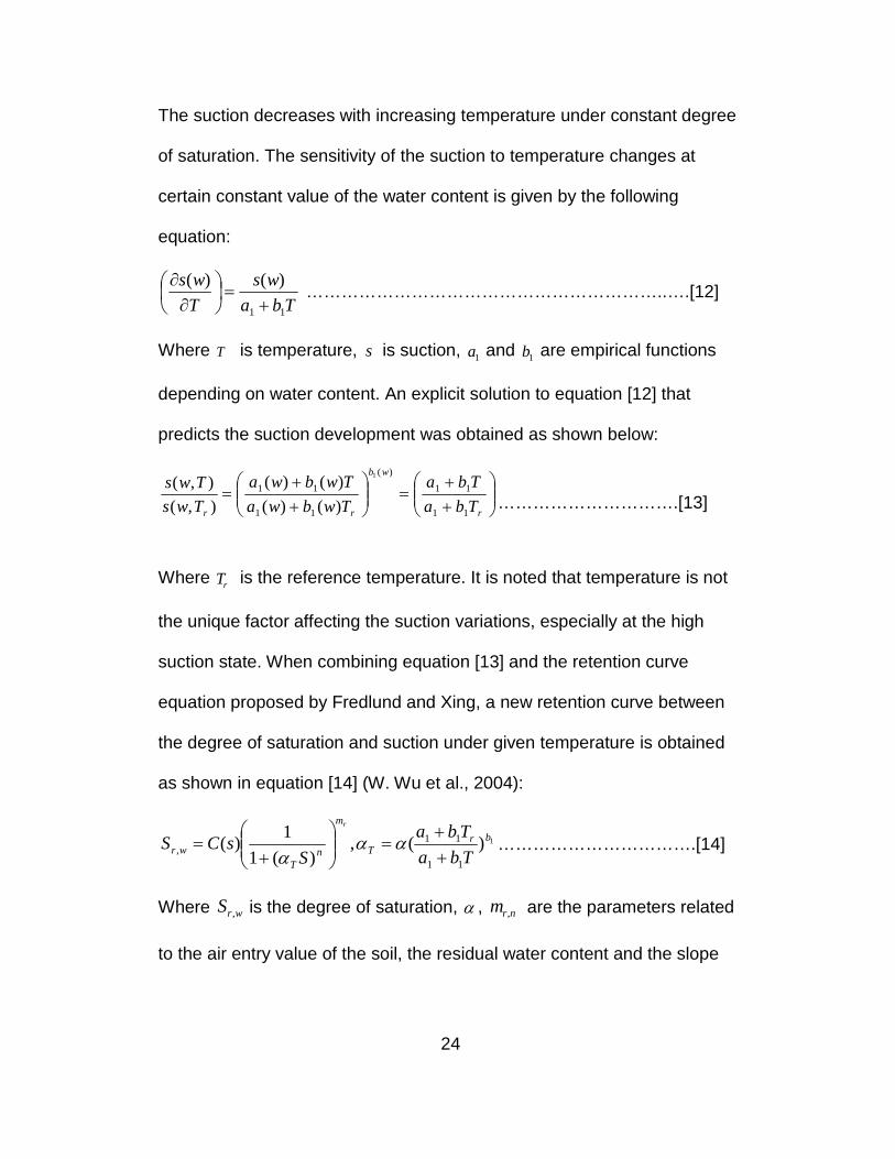
The suction decreases with increasing temperature under constant degree

of saturation. The sensitivity of the suction to temperature changes at

certain constant value of the water content is given by the following

equation:

Tba

ws

T

ws

11

)()(

+=

∂

∂ ……………………………………………………..….[12]

Where T is temperature, s is suction, 1a and 1b are empirical functions

depending on water content. An explicit solution to equation [12] that

predicts the suction development was obtained as shown below:

+

+=

+

+=

r

wb

rr Tba

Tba

Twbwa

Twbwa

Tws

Tws

11

11

)(

11

11

1

)()(

)()(

),(

),(………………………….[13]

Where rT is the reference temperature. It is noted that temperature is not

the unique factor affecting the suction variations, especially at the high

suction state. When combining equation [13] and the retention curve

equation proposed by Fredlund and Xing, a new retention curve between

the degree of saturation and suction under given temperature is obtained

as shown in equation [14] (W. Wu et al., 2004):

1)(,)(1

1)(

11

11,

brT

m

nT

wr Tba

Tba

SsCS

r

+

+=

+= αα

α…………………………….[14]

Where wrS , is the degree of saturation, α , nrm , are the parameters related

to the air entry value of the soil, the residual water content and the slope

25

of the suction-saturation curve at the air entry value of the soil,

respectively; and )(sC is a parameter related to suction.

Previous studies on the effect of temperature on the SWCC and their limitations Wenhua et al. (2004) conducted studies on the effect of temperature on

the SWCC. This research was conducted on compacted silt samples

using modified triaxial equipment. Isothermal and non-isothermal tests

were conducted. The temperature values applied were 25˚C, 40˚C, and

60˚C, and suction values varied from 0 to 300 kPa. Results from the

temperature controlled SWCC (soaking and desaturation) tests clearly

showed that the degree of saturation was reduced with increasing

temperature. This is due to the reduction of the surface tension of water

with increasing temperature, which in turn reduces the air entry value.

Owing to the air entry dependence of the effective stress, the effective

stress decreases with increasing temperature (Uchaipichat and Khalili

2009). These experiments were conducted in a suction ranging from 0 to

300 kPa, which is very limited. The effect of temperature on the SWCC at

higher suction values was not assessed even though it was suggested

that temperature had greater effect at low moisture content values.

The same authors also presented a case study on Boom clay. Results

showed that for a given water content, the total suction at 20oC was higher

than at 80oC due to the change in the capillary component of suction,

which was attributed to the change in surface tension of water, the change

26

in clay fabric, and the change in the pore-water chemistry of the clay. It is

worth noted that the change in clay fabric and the pore water chemistry

due to temperature changes is expected to be irreversible. This study

concluded that the change in clay fabric and the pore water chemistry do

not affect the total suction magnitude for clays with low organic content for

the range of temperatures used (20oC to 80oC); and therefore, the change

in total suction due to temperature may be caused by the change in the

capillary component of suction or the inaccuracy of the device used.

Models available for the temperature effect on the hydraulic conductivity Hydraulic conductivity is inversely proportional to the viscosity of the fluid.

The viscosities of fluids, including that of water, decrease proportionally to

the exponent of the reciprocal of temperature so that hydraulic

conductivity increases with increasing temperature. Therefore, the

absolute value of the matric potential decreases linearly with temperature

(Grant, 2005).

Empirical relations such as the van Genuchten equation relates soil water

content to matric potential:

( )n

n

neS

1

1

1−

+=

αψ…………………………………………………..…….[15]

Where eS is the water saturation defined by:

rs

reS

θθθθ−

−= ………………………………………………………………. [16]

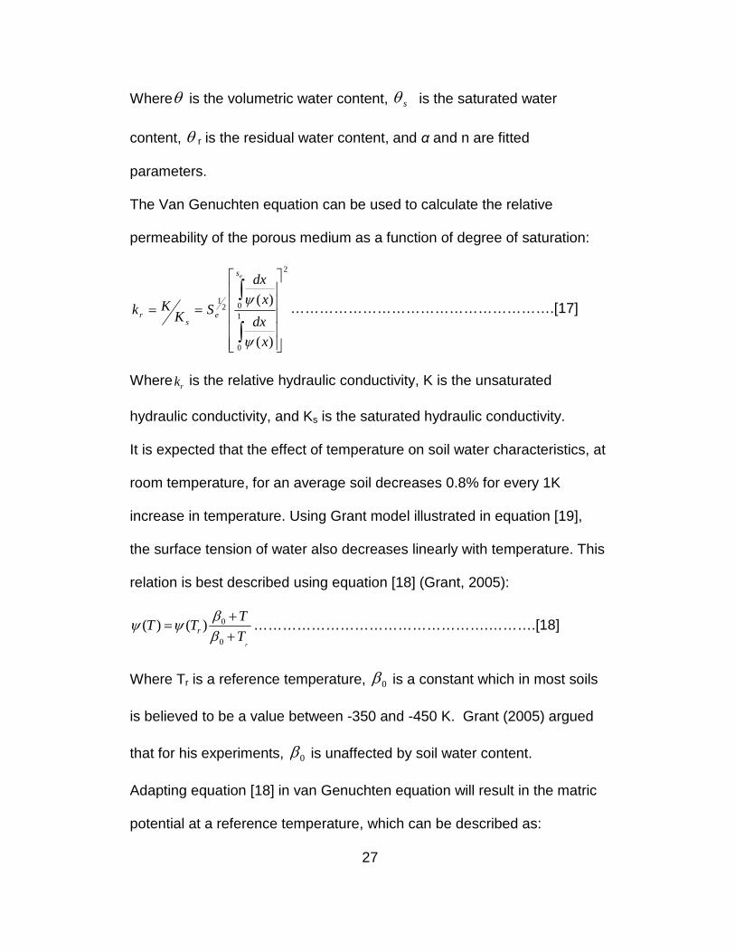
27

Whereθ is the volumetric water content, sθ is the saturated water

content, θ r is the residual water content, and α and n are fitted

parameters.

The Van Genuchten equation can be used to calculate the relative

permeability of the porous medium as a function of degree of saturation:

2

1

0

021

)(

)(

==

∫

∫

x

dx

x

dx

SKKk

es

es

r

ψ

ψ……………………………………………….[17]

Where rk is the relative hydraulic conductivity, K is the unsaturated

hydraulic conductivity, and Ks is the saturated hydraulic conductivity.

It is expected that the effect of temperature on soil water characteristics, at

room temperature, for an average soil decreases 0.8% for every 1K

increase in temperature. Using Grant model illustrated in equation [19],

the surface tension of water also decreases linearly with temperature. This

relation is best described using equation [18] (Grant, 2005):

rT

TTT r +

+=

0

0)()(ββ

ψψ ………………………………………….……….[18]

Where Tr is a reference temperature, 0β is a constant which in most soils

is believed to be a value between -350 and -450 K. Grant (2005) argued

that for his experiments, 0β is unaffected by soil water content.

Adapting equation [18] in van Genuchten equation will result in the matric

potential at a reference temperature, which can be described as:

28

n

n

n

r

e

TT

S

1

1

1

−

+

++

=

ββ

αψ

………………………………..………….[19]

Accordingly, the effect of increasing temperature is to decrease the matric

potential gradients (Grant, 2005).

Effect of temperature on hydraulic conductivity The hydraulic conductivity is directly proportional to liquid density, the

reciprocal of liquids viscosity, and the square of the mean grain diameter.

ηρgk

K = ……………………………………………………….……….[20]

Where � and η are the density and viscosity of the liquid, g is the

gravitational constant, and k is the intrinsic permeability of the porous

matrix

The water and the energy transport in a non-isothermal soil is governed by

the following equations:

z

KDTD

t WT ∂∂

−∇•∇+∇•∇=∂∂

)()( θθ

………………………………….[21]

)()( θ∇•∇−∇•∇=∂∂

wv DLTkt

TC ……………………………...……….[22]

Where t is the time in seconds, TD thermal water diffusivity, WD water

content –based water diffusivity, z depth, vC volumetric heat capacity, k

apparent thermal conductivity of the soil, and L latent enthalpy of

29

vaporization. The total volumetric water content is the sum of the liquid

and gas water contents. The use of these equations requires the

knowledge of four relationships to describe the properties of the soil in the

system (Mitchell and Soga, 2005): 1) hydraulic conductivity as a function

of water content; 2) thermal conductivity as a function of water content; 3)

volumetric heat capacity; and 4) suction head as a function of water

content. This approach is only applicable to homogenous and isotropic

porous media, and has several shortcomings: it assumes the soil volume

will remain constant, it cannot account for flow due to the changes in total

stress, and the water flow is in response to moisture content gradients

(rather than gradients in head), which implies that the soil is

homogeneous.

30

Chapter 4

ANALYSIS AND VALIDATION OF EXISTING MODELS This Chapter presents the analysis of the model presented by Grant in

2005. This model incorporates temperature effects on the SWCC as

presented before. In order to analyze the model, a database collected

from the NRCS was used. Details of the database and the analysis are

given below.

Database selection and processing

The database used to study the effect of temperature on soil water

retention contained around 4,800 surface soils from all over the USA. The

database was obtained from the National Resources Conservation

Service (NRCS). The NRCS has the objective of collecting, storing,

maintaining, and distributing the soil survey information for private land

owner in the United States, particularly the State Soil Geographic

(STATSGO) database. This data consist of soil map units that are linked

to attributes in order to indicate the location of each soil map unit and its

soil properties. The “map units” are areas that represent a group of soil

profiles with generally the same or similar characteristics.

The tabular data contained in the database represent a mean range of

properties for the soil comprised in each soil map unit. Information for

more than 9,000 soil profiles covering the entire United States were

31

collected and organized by Gustavo Torres at Arizona State University

(Torres, 2011).

The mean annual air temperature (MAAT) required for this analysis is not

included in this database. The GIS mapping system was used to locate

the soils in order to find out the MAAT. Once the longitude and latitude for

each sample was identified, the GIS mapping system was again used to

extract the MAAT for each soil.

Properties available for each soil unit

The soil properties included in the database to estimate the SWCC

parameters are the volumetric water content at 10, 33, and 1,500 kPa; and

the saturated volumetric water content (i.e., satiated water content or

porosity). In addition, parameters such as grain-size distribution values,

consistency limits, saturated hydraulic conductivity, groundwater table

depth and bedrock information were included.

Temperature effect evaluation The soils were divided into groups of similar properties. The properties

chosen to represent the soil were the percent passing #200 US sieve

(Passing200) and the Plasticity Index (PI). Soil families included soils with

Passing 200 ranging from 20-100% and PI value ranging from 0-12.5%.

Soil groups with PI values higher than 12.5% were considered, but the

data found did not have enough soils in different regions and therefore,

families of highly plastic soils were not available, as shown in Figures 6

32

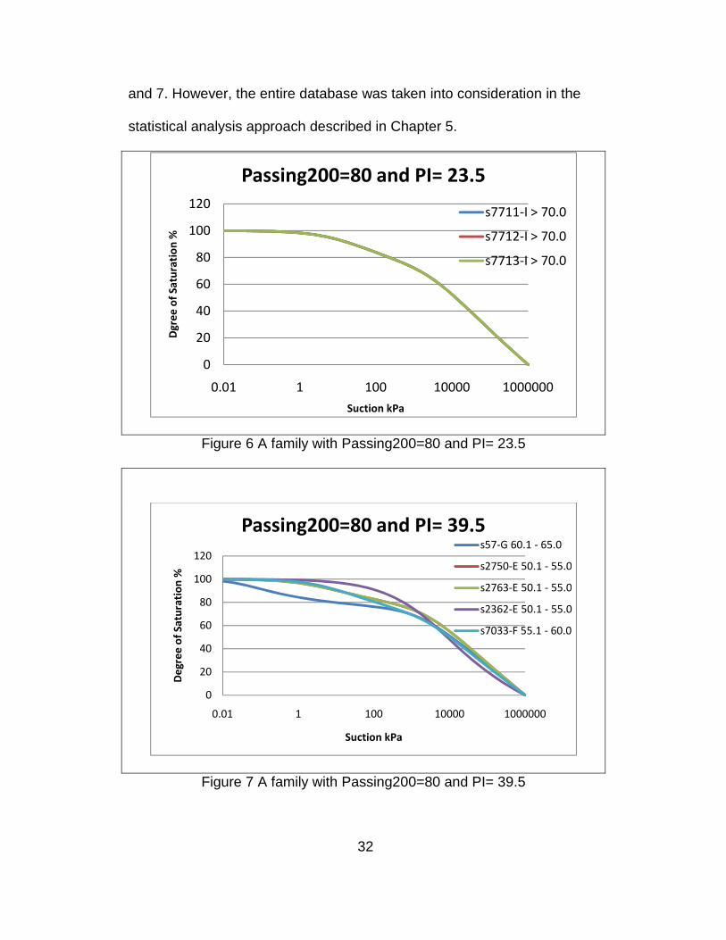
and 7. However, the entire database was taken into consideration in the

statistical analysis approach described in Chapter 5.

Figure 6 A family with Passing200=80 and PI= 23.5

Figure 7 A family with Passing200=80 and PI= 39.5

0

20

40

60

80

100

120

0.01 1 100 10000 1000000

Dg

ree

of

Sa

tura

tio

n %

Suction kPa

Passing200=80 and PI= 23.5

s7711-I > 70.0

s7712-I > 70.0

s7713-I > 70.0

0

20

40

60

80

100

120

0.01 1 100 10000 1000000

De

gre

e o

f S

atu

rati

on

%

Suction kPa

Passing200=80 and PI= 39.5s57-G 60.1 - 65.0

s2750-E 50.1 - 55.0

s2763-E 50.1 - 55.0

s2362-E 50.1 - 55.0

s7033-F 55.1 - 60.0

33

Twenty (20) groups were recognized to contain soil with similar index

properties. Each group included about 200 soils, but most of them were

located in the same region. For each group, the SWCC plots were drawn

and one or two representative soils were chosen for each location. In that

way, each group of soils was reduced to soils located in regions with

different mean annual air temperature (MAAT). The mean annual

temperature map for the US is presented in Figure 8. Soils representing

regions with MAAT as low as 30F and as high as 70F, and in between,

were included in the analysis.

Figure 8 Mean annual air temperature map (NOAA)

For each family of soils, the soil water characteristic curves were plotted

on the same graph to find any possible relation between MAAT and the

soil water characteristic curve. As stated before, each group consisted of

soils with similar PI and Passing200 values but different MAAT. By

keeping all other significant factors identical

effect of temperature.

More than 20 groups of soils were selected and plotted for this analysis. A

sample plot for a group of soils

shown in Figure 9. The graphs and tables

analysis are included in Appendix B.

Figure 9 SWCC

Results and analysis

Several observations were noted in these plots. Most significantly

inverse relationship between temperature and suction was observed.

Moreover, the effect of temperature

34

keeping all other significant factors identical, it was possible to isolate

More than 20 groups of soils were selected and plotted for this analysis. A

for a group of soils with PI = 7.5 and Passing200= 60

he graphs and tables for the 20 groups used in this

analysis are included in Appendix B.

SWCCs for Passing 200=60 and PI=7.5

were noted in these plots. Most significantly,

inverse relationship between temperature and suction was observed.

Moreover, the effect of temperature is more evident at lower degree of

it was possible to isolate the

More than 20 groups of soils were selected and plotted for this analysis. A

is

used in this

, a clear

inverse relationship between temperature and suction was observed.

degree of

35

saturation levels. Lastly, suction levels for soils with higher PI had notably

higher suction values.

Since the variation of suction due to temperature is not the same at

different degree of saturation levels; the degree of saturation level was

chosen to be 20%, as it represents the residual condition in soil.

Suction values at the 20% degree of saturation level for each soil in the

group were calculated using the Excel® goal seek function. The suction

was then plotted versus mean annual air temperature (MAAT) as shown in

Figure 10 and the relationship was modeled with the polynomial equation

for the curve. It was noted that the relations between temperature and

suction were different for groups with different PI value.

Figure 10 Relation between temperature and suction for soils with passing 200=60

Table 1 presents the equations found for each group of soils. The first

column shows the family of soil according to its passing 200 classification

y = 9E+07x-2.565

R² = 0.9477

0

2,000

4,000

6,000

8,000

10,000

12,000

14,000

16,000

20 25 30 35 40 45 50 55

Su

ctio

n (

kP

a)

Temperature (F)

Suction-Temperature Relationship For Soil Family (Passing200=60 , PI=7.5)

36

and the second column shows the range of PI values. For each PI value,

an equation was derived (third column) representing the relation between

temperature and suction for this particular family. The fourth column

shows the �� value for the equation. To calculate the suction from Grant

equation a reference temperature was needed. 70 degree F was chosen

to be the reference temperature used in Grant equation as noted in

column 5. The resulting suction calculated from the derived equations at

temperatures of 65, 60, 55, 50, 45, 40 F are presented in columns 6

through 11.

Comparison with Grant model for temperature effect on suction

In order to evaluate the effect of temperature versus that modeled in the

Grant equation, the suction values at the reference temperature were

calculated using the derived equations. Using this suction value as a

reference, the suction values at temperatures 40F, 45F, 50F, 55F, 60F

and 65F were calculated using the derived equation and the Grant

equation with 0β = -350K. Comparison plots were created for each soil

group as shown in Figure 11. For all groups of soils, it was observed that

the decrease in suction resulting from the increase in temperature was

greater in case of the derived equation, which suggested a smaller 0β

value than that proposed by Grant. It was also observed that 0β is not a

constant but a function of temperature.

37

Table 1 Comparison between existing and calculated equations

PI Derived Equation ��

suction at T=70F using equation

suction at T=65

suction at T=60

suction at T=55

suction at T=50

suction at T=45

suction at T=40

Passing 200 = 20

0 s = 2 x 1012 x T-5.894 0.6271 26.6699 41.3 66.2 110.5 193.8 360.6 721.9 2.5 s = 4 x 1016 x T-7.892 0.9998 109.8 197.0 370.6 736.4 1562.4 3588.4 9090.8 7.5 s = 1 x 1008 x T-2.456 0.9447 2940.6 3527.6 4294.0 5317.0 6719.4 8703.8 11623.6

Passing 200 = 30

0 s = 5 x 1022 x T-12.27 0.9934 1.5 3.8 10.1 29.3 93.7 338.7 1425.1

2.5 s = 2 x 1009 x T-3.348 0.8593 1329.4 1703.7 2227.3 2980.5 4100.9 5835.5 8656.3 5 s = 2 x 1010 x T-3.934 0.7315 1102.6 1475.8 2022.0 2847.4 4142.7 6270.4 9966.1

Passing 200 = 40

2.5 s = 8x 1010 x T-4.235 0.8013 1227.7 1680.4 2358.4 3409.2 5104.5 7975.1 13133.1

5 s = 91056 x T-0.82 0.1234 2794.7 2969.7 3171.2 3405.7 3682.6 4014.9 4422.0

7.5 s = 1x 1010 x T-3.567 0.9364 2621.4 3414.6 4542.9 6196.2 8705.1 12676.3 19295.3

Passing 200 = 50

2.5 s = 144.92 x T-0.139 0.966 80.3 81.1 82.0 83.0 84.1 85.4 86.8 5 s = 3 x 1008 x T-2.824 0.9872 1847.4 2277.5 2855.1 3650.4 4777.8 6433.5 8972.3

12.5 s = 2 x 1008 x T-2.443 0.8014 6215.2 7448.7 9057.5 11202.7 14139.9 18290.8 24389.2

Passing 200 = 60

3.5 s = 3 x 1011 x T-4.874 0.7921 304.9 437.5 646.3 987.6 1571.6 2626.4 4663.2 5 s = 5 x 1006 x T-1.764 0.9218 2781.1 3169.5 3650.2 4255.7 5034.9 6063.2 7463.4

7.5 s = 9 x 107 x T-2.565 0.9477 1665.6 2014.3 2473.3 3091.8 3948.1 5173.1 6997.8

Passing 200 = 70

5 s = 2 x 106x T-1.427 0.6896 4656.7 5176.1 5802.4 6569.5 7526.6 8747.7 10348.8 9-10 s = 106193 x T-0.555 0.1086 10047.7 10469.6 10945.2 11486.7 12110.6 12839.9 13707.3

Passing 200 = 80

7.5 s = 8 x 1011x T-4.68 0.6856 2604.0 3661.7 5291.7 7896.3 12241.3 19875.2 34167.5

10 s = 7 x 1011 x T-4.434 0.8012 4612.5 6406.8 9136.4 13437.9 20505.3 32715.5 55152.3

38

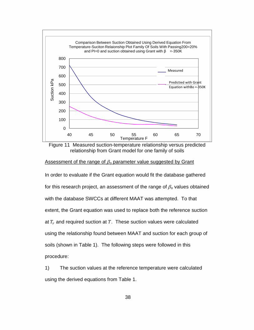
Figure 11 Measured suction-temperature relationship versus predicted

relationship from Grant model for one family of soils

Assessment of the range of βo parameter value suggested by Grant

In order to evaluate if the Grant equation would fit the database gathered

for this research project, an assessment of the range of βo values obtained

with the database SWCCs at different MAAT was attempted. To that

extent, the Grant equation was used to replace both the reference suction

at �� and required suction at �. These suction values were calculated

using the relationship found between MAAT and suction for each group of

soils (shown in Table 1). The following steps were followed in this

procedure:

1) The suction values at the reference temperature were calculated

using the derived equations from Table 1.

0

100

200

300

400

500

600

700

800

40 45 50 55 60 65 70

Suc

tion

kPa

Temperature F

Comparison Between Suction Obtained Using Derived Equation From Temperature-Suciton Relaionship Plot Family Of Soils With Passing200=20%

and PI=0 and suction obtained using Grant with βₒ =-350K

Predictied with Grant

Equation withBo =-350K

Measured

39

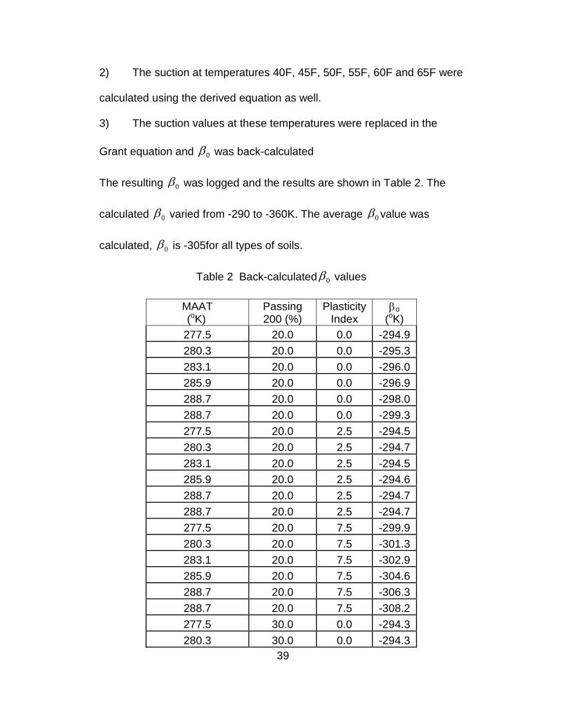
2) The suction at temperatures 40F, 45F, 50F, 55F, 60F and 65F were

calculated using the derived equation as well.

3) The suction values at these temperatures were replaced in the

Grant equation and 0β was back-calculated

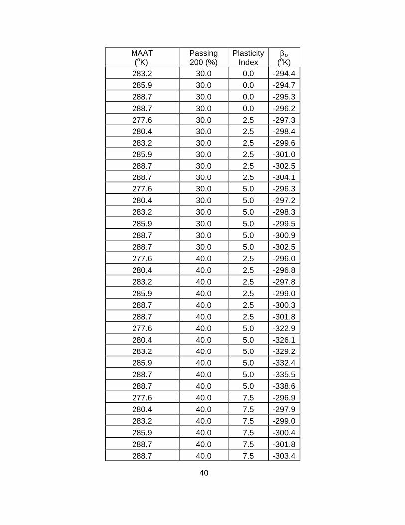
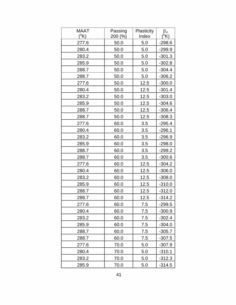
The resulting 0β was logged and the results are shown in Table 2. The

calculated 0β varied from -290 to -360K. The average 0β value was

calculated, 0β is -305for all types of soils.

Table 2 Back-calculated 0β values

MAAT (oK)

Passing 200 (%)

Plasticity Index

βo

(oK) 277.5 20.0 0.0 -294.9

280.3 20.0 0.0 -295.3

283.1 20.0 0.0 -296.0

285.9 20.0 0.0 -296.9

288.7 20.0 0.0 -298.0

288.7 20.0 0.0 -299.3

277.5 20.0 2.5 -294.5

280.3 20.0 2.5 -294.7

283.1 20.0 2.5 -294.5

285.9 20.0 2.5 -294.6

288.7 20.0 2.5 -294.7

288.7 20.0 2.5 -294.7

277.5 20.0 7.5 -299.9

280.3 20.0 7.5 -301.3

283.1 20.0 7.5 -302.9

285.9 20.0 7.5 -304.6

288.7 20.0 7.5 -306.3

288.7 20.0 7.5 -308.2

277.5 30.0 0.0 -294.3

280.3 30.0 0.0 -294.3

40

MAAT (oK)

Passing 200 (%)

Plasticity Index

βo

(oK) 283.2 30.0 0.0 -294.4

285.9 30.0 0.0 -294.7

288.7 30.0 0.0 -295.3

288.7 30.0 0.0 -296.2

277.6 30.0 2.5 -297.3 280.4 30.0 2.5 -298.4

283.2 30.0 2.5 -299.6 285.9 30.0 2.5 -301.0

288.7 30.0 2.5 -302.5

288.7 30.0 2.5 -304.1

277.6 30.0 5.0 -296.3

280.4 30.0 5.0 -297.2

283.2 30.0 5.0 -298.3

285.9 30.0 5.0 -299.5

288.7 30.0 5.0 -300.9

288.7 30.0 5.0 -302.5

277.6 40.0 2.5 -296.0

280.4 40.0 2.5 -296.8

283.2 40.0 2.5 -297.8

285.9 40.0 2.5 -299.0

288.7 40.0 2.5 -300.3

288.7 40.0 2.5 -301.8

277.6 40.0 5.0 -322.9

280.4 40.0 5.0 -326.1

283.2 40.0 5.0 -329.2

285.9 40.0 5.0 -332.4

288.7 40.0 5.0 -335.5

288.7 40.0 5.0 -338.6

277.6 40.0 7.5 -296.9

280.4 40.0 7.5 -297.9

283.2 40.0 7.5 -299.0

285.9 40.0 7.5 -300.4

288.7 40.0 7.5 -301.8

288.7 40.0 7.5 -303.4

41

MAAT (oK)

Passing 200 (%)

Plasticity Index

βo

(oK) 277.6 50.0 5.0 -298.6

280.4 50.0 5.0 -299.9

283.2 50.0 5.0 -301.3

285.9 50.0 5.0 -302.8

288.7 50.0 5.0 -304.4 288.7 50.0 5.0 -306.2

277.6 50.0 12.5 -300.0

280.4 50.0 12.5 -301.4

283.2 50.0 12.5 -303.0

285.9 50.0 12.5 -304.6

288.7 50.0 12.5 -306.4

288.7 50.0 12.5 -308.3

277.6 60.0 3.5 -295.4

280.4 60.0 3.5 -296.1

283.2 60.0 3.5 -296.9

285.9 60.0 3.5 -298.0

288.7 60.0 3.5 -299.2

288.7 60.0 3.5 -300.6

277.6 60.0 12.5 -304.2

280.4 60.0 12.5 -306.0

283.2 60.0 12.5 -308.0

285.9 60.0 12.5 -310.0

288.7 60.0 12.5 -312.0

288.7 60.0 12.5 -314.2

277.6 60.0 7.5 -299.5

280.4 60.0 7.5 -300.9

283.2 60.0 7.5 -302.4

285.9 60.0 7.5 -304.0

288.7 60.0 7.5 -305.7

288.7 60.0 7.5 -307.5

277.6 70.0 5.0 -307.9

280.4 70.0 5.0 -310.1

283.2 70.0 5.0 -312.3

285.9 70.0 5.0 -314.5

42

MAAT (oK)

Passing 200 (%)

Plasticity Index

βo

(oK) 288.7 70.0 5.0 -316.8

288.7 70.0 5.0 -319.2

277.6 70.0 10.0 -340.0

280.4 70.0 10.0 -344.2

283.2 70.0 10.0 -348.4 285.9 70.0 10.0 -352.4

288.7 70.0 10.0 -356.5 288.7 70.0 10.0 -360.4

277.6 80.0 7.5 -295.6

280.4 80.0 7.5 -296.4

283.2 80.0 7.5 -297.3

285.9 80.0 7.5 -298.4

288.7 80.0 7.5 -299.6

288.7 80.0 7.5 -301.1

277.6 80.0 10.0 -295.8

280.4 80.0 10.0 -296.5

283.2 80.0 10.0 -297.5

285.9 80.0 10.0 -298.6

288.7 80.0 10.0 -299.9

288.7 80.0 10.0 -301.0

Summary and conclusions

Data on soils in the NRCS was processed to obtain the MAAT for each

sample. Groups of soils with similar properties but different MAAT were

grouped and the SWCCs for each group of soils were plotted. A clear

inverse relationship between temperature and suction was observed.

From visual inspection, the effect of temperature was found to be more

discernable at lower degree of saturation levels. Lastly, suction levels for

soils with higher PI had notably higher suction values.

43

Based on the relationship between temperature and suction found for the

soils in the database, the results were compared to the suction values

define by Grant equation, by using the back-calculation of the βo

parameter. It was noticed that even though the temperature effect followed

the same trend as the model, it had a slightly more profound effect on

suction as that calculated by the Grant equation. The results suggested

that the 0β value in the Grant equation can be refined by reducing it to -

305K from the -350- -450K suggested by Grant (Grant, 2005).

44

Chapter 5

STATISTICAL ANALYSIS MODEL

Suction model using statistical analysis

Sample soil selection and procedure

Statistical analysis was used to provide an accurate suction model and

analyze its dependence on temperature as well as PI, and passing200

values. In order to create the database that represents a wide variation in

all of these factors, the same database used in chapter 4 comprising of

more than 9,000 soils with various PI, passing200, temperatures and

suction values was used. The database did not include the suction value

at 20% degree of saturation level needed for this analysis. An Excel®

macro was created to determine the suction value for each soil at 20%

degree of saturation level. The macro used the goal seek function in

Excel® for multiple cells to determine the suction. Soils with missing

temperature or suction values were then excluded and the database

referenced in appendix A was fed to Minitab®. The cleaned up version of

the data base still represented approximately 4,800 soils. The soils

locations are presented in Figure 12

45

Figure 12 Soils distribution map used in the statistical analysis

Statistical analysis and results

The data obtained from the NRCS database was processed in Minitab®

regression analysis model to obtain the predicted suction equation. The

best model found is given by:

s = - 196 – 29.7 MAAT + 1483 PI + 14.65 Passing200………………….[23]

Where s is the suction at 20% degree of saturation, MAAT is the mean

annual air temperature, PI is the soil plasticity index, and the passing 200

is the percentage of soil passing through sieve number 200.

The screenshot from Minitab is shown in Figure 13. The coefficient of

determination (R-square) was found to be 71.4%, which proves that the

data points fit the model relatively well. The P value is also an indicator of

how statistically significant each factor is in calculating suction. The lower

the P value the more statistically significant the factor is. With this in mind

46

the suction value was found to be largely dependent on PI with a P value

of 0.00. The next most significant factor was found to be the temperature

value and lastly the Passing200.

Figure 13 Minitab(R) regression analysis output

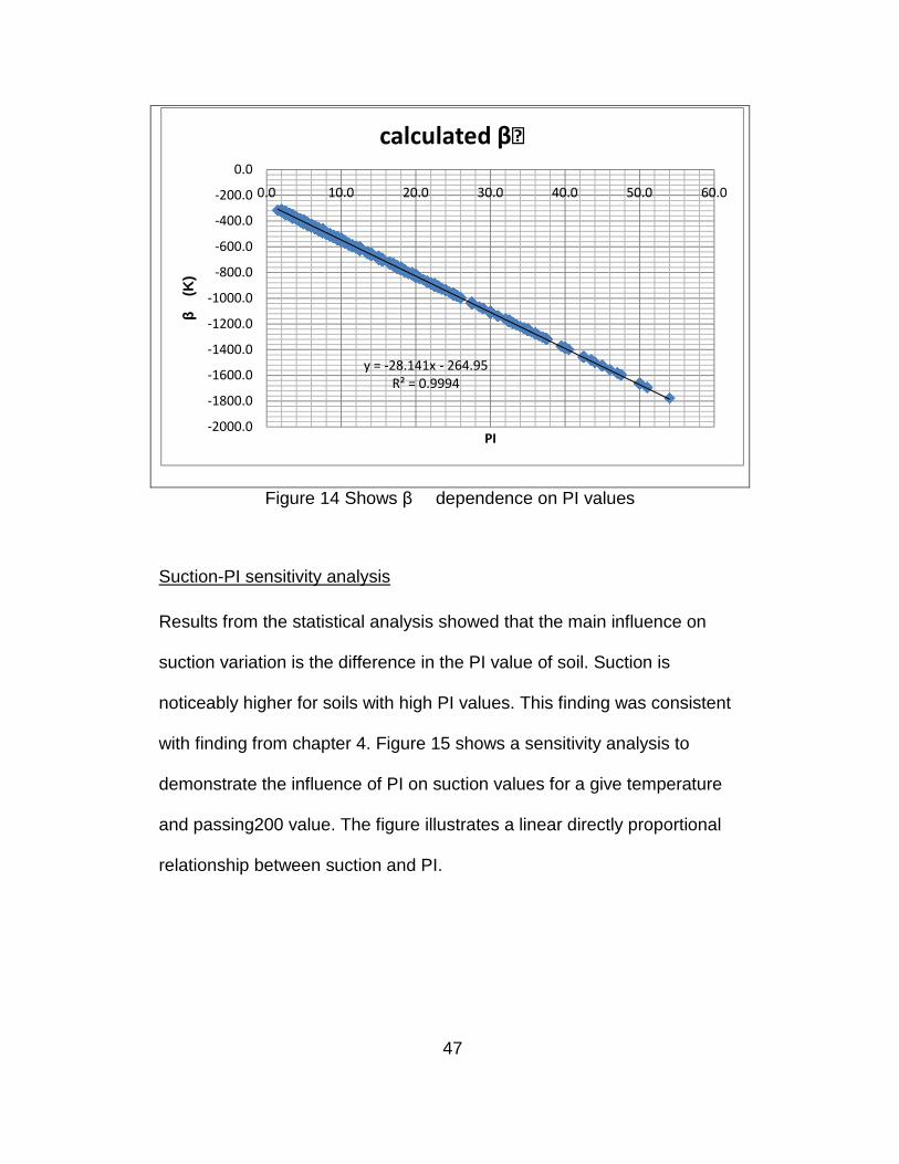
βₒ - PI relationship The model was used to calculate the βₒ values for the whole database.

This was done by initially calculating suction at both the reference

temperature (70F) and the minimum temperature (30F) using the

statistical analysis model. The suction values were then replaced in the

Grant equation and the βₒ was calculated. Appendix C shows the

calculated βₒ values. βₒ showed strong dependence on PI values. The

βₒ is linearly inversely proportional to the PI value as illustrated in Figure

14.

47

Figure 14 Shows βₒ dependence on PI values

Suction-PI sensitivity analysis

Results from the statistical analysis showed that the main influence on

suction variation is the difference in the PI value of soil. Suction is

noticeably higher for soils with high PI values. This finding was consistent

with finding from chapter 4. Figure 15 shows a sensitivity analysis to

demonstrate the influence of PI on suction values for a give temperature

and passing200 value. The figure illustrates a linear directly proportional

relationship between suction and PI.

y = -28.141x - 264.95

R² = 0.9994

-2000.0

-1800.0

-1600.0

-1400.0

-1200.0

-1000.0

-800.0

-600.0

-400.0

-200.0

0.0

0.0 10.0 20.0 30.0 40.0 50.0 60.0βₒ

(K

)

PI

calculated βₒ

48

Figure 15 Effect of temperature on suction for different PI values

Suction_Passing200 Sensitivity Analysis

Another factor affecting the suction values in soils is the passing200 value.

A sensitivity analysis was performed using the equation 23 to isolate the

effect of the passing200 value on soil suction. Figure 16 illustrates a

directly proportional, linear relationship between passing200 and suction.

However, the influence of the passing200 level on soil suction was shown

to be much less of that of the PI value.

Suction-PI sensitivity analysis

1000

6000

11000

16000

21000

26000

31000

36000

41000

46000

51000

0 5 10 15 20 25 30 35

PI value

Su

ctio

n

suction Per Equation T=40 suction Per Equation T=45 suction Per Equation T=50 suction Per Equation T=55 suction Per Equation T=60 suction Per Equation T=65 suction Per Equation T=70

49

Figure 16 Effect of temperature on suction with different passing 200

Summary and conclusions

Results obtained from the statistical analysis on approximately 4,800 soil

sample and using Minitab® were in line with the result obtained in chapter

4 using derived equations for each group of soil. This approach was

proven to be better not only because of the accuracy of the software used

but also because it allowed the created of model that captures the

temperature effect along with other important soil properties in the same

equation. The analysis showed that the temperature effect on suction is

lower than that of soil properties such as the PI value. However, the effect

of temperature was large enough not to be ignored.

suction-passing 200 sensitivity analysis

4000

4500

5000

5500

6000

6500

7000

7500

8000

0 20 40 60 80 100 120

passing 200

suct

ion

kP

a

suction Per Equation T=40

suction Per Equation T=45

suction Per Equation T=50

suction Per Equation T=55

suction Per Equation T=60

suction Per Equation T=65

suction Per Equation T=70

50

Chapter 6

STATISTICAL ANALYSIS MODEL USING TMI

Introduction to Thornthwaite Moisture Index

The Thornthwaite Moisture Index was found to be the most significant parameter for predicting suction under pavements. In 1948, Thornthwaite

introduced the TMI as an index that classified the climate of a given

location (McKeen and Johnson 1990). The TMI quantifies the aridity or

humidity of a soil-climate system by summing the effects of annual

precipitation, evapotranspiration, storage, deficit and runoff.

The TMI values for a region can be estimated from the contour map. For

the analysis presented here, the TMI value for each sample was obtained

from the TMI contour map shown in Figure 17 (FHWA-RD-90-033, 1990)

Figure 17 Thornthwaite Moisture Index Contour Map

51

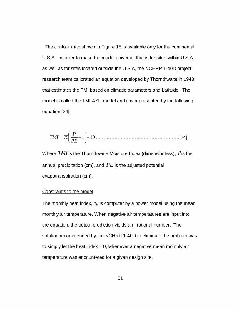
. The contour map shown in Figure 15 is available only for the continental

U.S.A. In order to make the model universal that is for sites within U.S.A.,

as well as for sites located outside the U.S.A, the NCHRP 1-40D project

research team calibrated an equation developed by Thornthwaite in 1948

that estimates the TMI based on climatic parameters and Latitude. The

model is called the TMI-ASU model and it is represented by the following

equation [24]:

10175 +

−=PE

PTMI ………………………..…………………….[24]

Where TMI is the Thornthwaite Moisture Index (dimensionless), Pis the

annual precipitation (cm), and PE is the adjusted potential

evapotranspiration (cm).

Constraints to the model

The monthly heat index, hi, is computer by a power model using the mean

monthly air temperature. When negative air temperatures are input into

the equation, the output prediction yields an irrational number. The

solution recommended by the NCHRP 1-40D to eliminate the problem was

to simply let the heat index = 0, whenever a negative mean monthly air

temperature was encountered for a given design site.

52

Previous studies showed soil suction beneath paved areas is governed by

the regional TMI and the percentage of fines present in the soil, as the

suction increase the TMI value decrease. TMI represents the climatic

condition, effect of temperature, precipitation, solar radiation, and the type

of soil (Yugantha, 2003).

Minitab Analysis

Another statistical analysis was used to model the effect of TMI along with

PI and Passing200 values on the suction level. The database provided in

the table below was used to in Minitab® to analyze the TMI effect. The

output from Minitab is shown in Figure 18. The output equation from

Minitab® was:

S= -6137 - 30.2 passing 200 +964PI + 29.6 TMI……………………….[25]

Where S is the suction, passing 200 is the percentage passing from sieve

number 200, PI is the soil plasticity index, and TMI is the Thornthwaite

moisture index.

The equation indicated a directly proportional relationship between the

suction value and the TMI.

Regression Analysis: Suction versus Passing 200, PI, and TMI

53

Figure 18 Regression analysis for TMI versus suction

Summary and conclusion

The statistical analysis of the influence on TMI on soil suction showed a

much less than that of temperature. Difficulties in obtaining the TMI values

for a large number of soil samples in the database prevented using an

adequate sample size as that used in the temperature effects analysis.

Only 28 soils were used in the TMI study which may have affected the

accuracy of the analysis as indicated in the R-squared value of 54.1%

from Minitab®.

54

Chapter 7

CONCLUSION AND RECOMMENDATION FOR FUTURE WORK

Conclusion with respect to the Grant equation

In recent years the increase in geotechnical engineering applications is

becoming wider, especially in the geo-environmental area. As a result,

new problems require the extension of current understanding of soil

behavior with the description of new phenomena and the incorporation of

the environmental variables. The new applications are mainly relate to the

effect of temperature change on partially saturated soils. The first

technique used to assess the effect of temperature on the soil water

characteristic curve included the validation of an existing model making

use of a large database. The empirical van Genuchten expression

incorporates the effect of temperature on matric potential as described by

the following relation:

r

T

TTT r +

+=

0

0)()(ββ

ψψ ……………………………………………………….[24]

Where βₒ was proposed to be a constant varying between -350K and -

450K for most soils. However, the model did not specify any dependence

of βₒ on soil properties. This model was validated by using the existing

database. Similar soils in different locations all over the United States

were gathered in groups of similar soil properties with different mean

annual air temperature, or each family of soils the soil water retention

55

curves were plotted at different temperature. For all families plotted there

was a clear trend between suction and temperature. The trend was only

clear at lower level of degree of saturations, and it is very significant at

20% degree of saturation. The effect of increasing temperature is to

decrease the matric potential. Also using the same approach the βₒ, a

strong dependence of βₒ on PI value was observed and modeled. The

value of βₒ decreased linearly with the increase in PI.

Conclusion with respect to statistical model to incorporate the temperature

effect on suction

This approach was followed in order to analyze soils at different locations

with the same soil properties and different mean annual air temperature.

The soils used in this approach were about 4,800 soils. After calculating

the soils suction, Minitab software was used to run the analysis. The

analysis provided a clear relation between suction, temperature, soil

plasticity index and the percent passing #200 US sieve. A sensitivity

analysis on the statistical model obtained indicates that as the

temperature decreases the suction increase; and as the PI and passing

200 increase the suction increases.

56

The model was used to calculate the βₒ values for the whole database.

This was done by initially calculating suction at both the reference

temperature (70F) and the minimum temperature (30F) using the

statistical analysis model. The suction values were then replaced in the

Grant equation and the βₒ was calculated. The calculated βₒ values

showed strong dependence on PI values. The βₒ is linearly inversely

proportional to the PI value

Conclusion with respect to statistical model to incorporate the TMI effect

on suction

The statistical analysis of the influence on TMI on soil suction showed a

much less than that of temperature. Difficulties in obtaining the TMI values

for a large number of soil samples in the database prevented using an

adequate sample size as that used in the temperature effects analysis.

Only 28 soils were used in the TMI study which may have affected the

accuracy of the analysis as indicated in the R-squared value of 54.1%

from Minitab®.

Recommendation for future work

The incorporation of the temperature effect in soil retention has not been

taking into consideration in the past, but as the increasing trend of

geotechnical applications requiring its inclusion continues, a further

57

understanding of the temperature effect on moisture retention is required.

The model validated as well as the proposed model in this study show the

temperature effect on suction is minimal compared to the soil properties

effect, but should not be neglected and should be taking into

consideration, especially when applied to barriers for nuclear waste

storage and (ET) covers for municipal solid waste containment.

Future research should be done in the laboratory under controlled

conditions to validate the findings of this study.

58

REFERENCES

Bacchi, O.O.S., Reichardt, K., Oliveira, J.C.M., Nielsen, D.R.

bulk density, and limited data. Soil Sci. 153, 172–184,1992

Croney, D., and Coleman, J.D. pore pressure and suction in soil. In

proceedings, conference on pore pressure and suction in soils.

Butterworth, London. Pp.31-37, 1960

Duarte, A.P.L., de Campos, T.M.P., Araruna Jr., J.T. and Rocha

Filho, P. Thermal Properties for Unsaturated Soils. Unsaturated Soils .

Geotechnical Special Publication No. 147. The Geo-Institute of the ASCE.

Proceedings of the 4th International Conference on Unsaturated Soils.

April 2-6, Carefree, AZ, 1707-1718, 2006

Fredlund, D.G. and Xing, A. Equation for the soil–water

characteristic curve. Can Geotech J. 1994

Fredlund, D.G., and Rahardjo, H. Soil mechanics for

Gamma-ray beam attenuation as an auxiliary technique for

Grifoll, J., Gasto, J.M. and Cohen, Y. Non-isothermal soil water

transport and evaporation. Advances in Water Resources 28 (2005)

1254–1266

Habibagahi, K. temperature effect and the concept of effective void

ratio. Indian Geotech J, 1:14-34, 1997

59

Hopmans JW and Dane JH. Temperature dependence of soil

hydraulic properties. Soil Sci Soc Am J;50:4-9 1986.

Jacinto, A.C., Gómez-Espina, R., Villar, M.V. and Ledesma, A.

Adaptation of the van Genuchten expression to the effects of temperature

and density for compacted bentonites. Applied Clay Science, Volume 42,

Issues 3-4, 575-582, 2009

Khanzode, R.M., Vanapalli, S.K., Fredlund, D.G., Pufahl, D.E., and

Clifton, A.W.Measurement of soil-water characteristic curves

for fine-grained soils using a small-scale centrifuge. Canadian

Geotechnical Journal, 2002.

Liu, H.H. and Dane, J.H. Reconciliation between measured and

theoretical temperature effects on soil water retention curves. Soil Sci Soc

Am J ;57:1202-7,1993

Mitchell JK. Fundamentals of soil behaviour. New York: Wiley;

1993.

NOAA, Mean annual air temperature map,

http://www.ncdc.noaa.gov/oa/fpsf/fpsfmaps.html (last accessed: July

2011).

Perera, Y. Y. “Moisture Equilibria beneath Paved Areas.” PhD

Dissertation, Arizona State University, Arizona, USA. 2003

Philip, J.R. and de Vries, D.A., Moisture movement in porous

materials under temperature gradients. Trans. Am. Geophysics. Union,

38(2): 222-232,1957

60

Puppala, A.J., Punthutaecha, K. and Vanapalli, S.K. Soil-Water

Characteristic Curves of Stabilized Expansive Soils. Journal of

Geotechnical and Geoenviromental Engineering, ASCE, 132(6), 736-75,

2006

Rahardjo H., Leong E. C. Suction measurements. Proc. 4th Int.

Conf. on Unsaturated Soils, Carefree, AZ. 562-7, 2006

Richards. B.G. Measurement of the free energy of soil moisture by

the psychrometric technique using thermistors. In Moisture equilibria and

moisture changes in soils beneath covered areas. Edited by G.D.

Aitchison. Butterworth & Co. Ltd., Sydney, Australia, pp. 39-46,1965

Romero E, and Gens A. Characterization and thermo-hydro-

mechanical behaviour of unsaturated Boom clay: an experimental study.

Doctoral Thesis, Technical University of Catalonia (UPC), Barcelona,

Spain, 1999

She HY and Sleep BE. The effect of temperature on capillary

pressure-saturation relationships for air-water and perchloroethylene-

water systems. Water Resour Res 34 (10):2587-2597, 1998

Simms, P.H., Yanful, E.K., St-Arnaud, L. and Aubé, B. A laboratory

evaluation of metal release and transport in flooded pre-oxidized mine

tailings. Applied Geochemistry, 15: 1245-1263, 2000

the evaluation of soil water retention curve. Sci. Agric.55,499–502, 1998

61

Tang, X., J. Graham, and A.W.L. Wan. 1997. Measuring total

suctions by psychrometer in triaxial tests. p. 213–216. In Proceedings of

the XIVth International Conference on Soil Mechanics and Foundation

Engineering, Hamburg, Germany. Vol. 1.

Torres-Hernandez, G. Estimating the Soil–Water Characteristic

Curve Using Grain Size Analysis and Plasticity Index. Master of Science

Thesis, Arizona State University, Tempe, AZ, USA, 2011.

Uchaipichat, A. and Khalili, N. Experimental investigation of

thermo-hydro-mechanical behavior of an unsaturated silt. Geotechnique

59, No. 4, 339-353, 2009

Van Genuchten, M.Th. Calculating the unsaturated hydraulic

conductivity with a new form analytical model. Res. Rep. 78-WR-08,

Water Resources Program, Department of Civil Engineering, Princeton

University, Princeton, NJ, 1999.

Van Genuchten, M.Th.,. A closed-form equation for predicting the

hydraulic conductivity of unsaturated soils. Soil Sci. Soc. Am.,1980.

Vanapalli, S.K, and Fredlund, D.G , Empirical procedures to predict

the shear strength of unsaturated soils, university of Saskatchewan, 1996.

Wenhua, W., Xilkui Li, F. and Collin, A. Thermo-hydro-mechanical

model and its numerical modeling for unsaturated soil. Computers and

Geotechnical 31,155-167, 2004

62

Williams, R.D., Ahuja, L.R., and Naney, J.W. Comparison of

methods to estimate soil water characteristics from soil texture

unsaturated soils. John Wiley & Sons, Inc., New York, 1993

Witczak, M.W., Zapata, C.E., and Houston, W.N. (2006). Models

Incorporated into the Current Enhanced Integrated Climatic Model:

NCHRP 9-23, Project Findings and Additional Changes after Version 0.7.

Final Report Project NCHRP 1-40D. Inter Team Technical Report. Arizona

State University, Tempe.

Zapata, C.E. Uncertainty in soil- water- characteristic curve and

impacts on unsaturated shear strength predictions. Doctoral thesis.

Arizona State University, Tempe AZ, USA. 1999

63

APPENDIX A

SWCC PLOTS FOR SOIL GROUPS WITH SAME CHARACTERISTICS

AT DIFFERENT TEMPERATURES

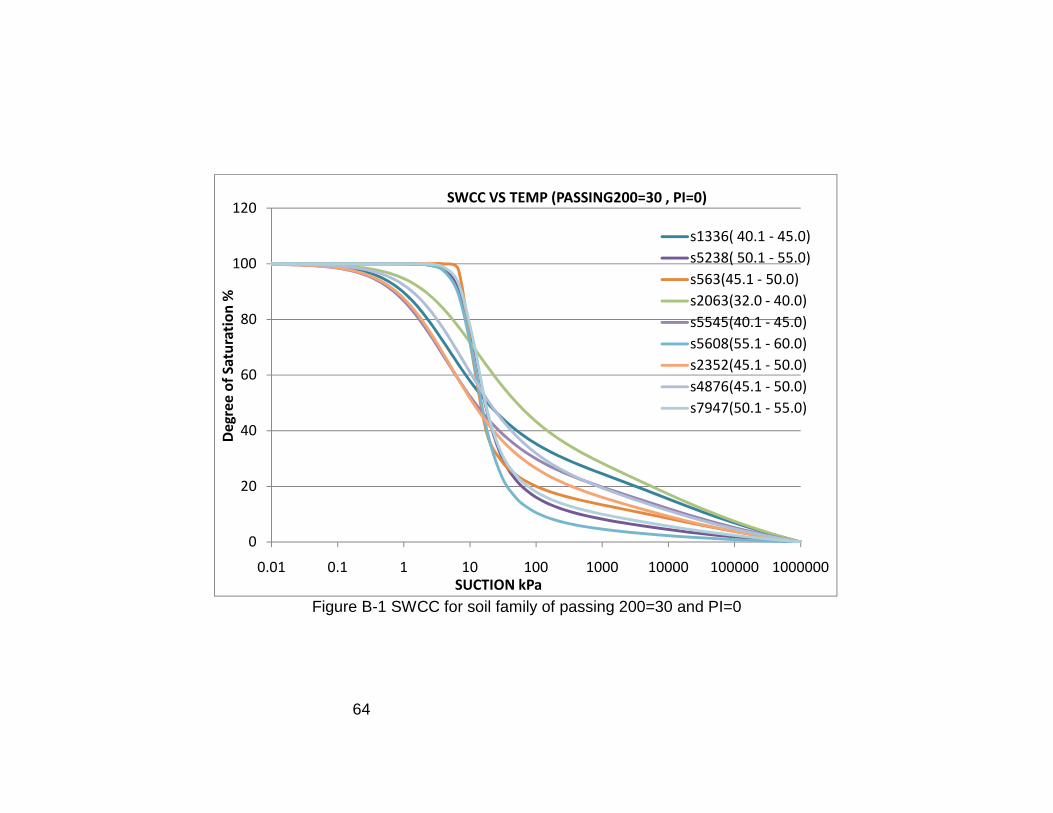
64

Figure B-1 SWCC for soil family of passing 200=30 and PI=0

0

20

40

60

80

100

120

0.01 0.1 1 10 100 1000 10000 100000 1000000

De

gre

e o

f S

atu

rati

on

%

SUCTION kPa

SWCC VS TEMP (PASSING200=30 , PI=0)

s1336( 40.1 - 45.0)

s5238( 50.1 - 55.0)

s563(45.1 - 50.0)

s2063(32.0 - 40.0)

s5545(40.1 - 45.0)

s5608(55.1 - 60.0)

s2352(45.1 - 50.0)

s4876(45.1 - 50.0)

s7947(50.1 - 55.0)

65

Figure B-2 SWCC for soil family of passing 200=30 and PI=2.5

0

20

40

60

80

100

120

0.01 1 100 10000 1000000

De

gre

e o

f S

atu

rati

on

%

SUCTION kPa

SWCC VS TEMP (PASSING200=30 , PI=2.5)

s130(60.1 - 65.0)

s295(65.1 - 70.0)

s363(50.1 - 55.0)

s1250(45.1 - 50.0)

s1337(40.1 - 45.0)

s5090(45.1 - 50.0)

s5153(32.0 - 40.0)

s550( 40.1 - 45.0)

s6458(60.1 - 65.0)

s9114(40.1 - 45.0)

66

Figure B-3 SWCC for soil family of passing 200=30 and PI=5

0

20

40

60

80

100

120

0.01 1 100 10000 1000000

De

gre

e o

f S

atu

rati

on

%

SUCTION kPa

SWCC VS TEMP (PASSING200=30 , PIi=5)

s1487(60.1 - 65.0)

s1659(65.1 - 70.0)

s7634(> 70.0)

s7862(50.1 - 55.0)

s8132(45.1 - 50.0)

s8149(45.1 - 50.0)

s4215(32.0 - 40.0)

s4414(45.1 - 50.0)

67

Figure B-4 for soil family of passing 200=30 and PI=7.5

0

20

40

60

80

100

120

0.01 1 100 10000 1000000

De

gre

e o

f S

atu

rati

on

SUCTION (KPa)

SWCC VS temp (Passing 200=30 , PI=7.5)

s1351(32.0 - 40.0)s5488(50.1 - 55.0)s5536(40.1 - 45.0)s5833(45.1 - 50.0)s5849(45.1 - 50.0)s7935(40.1 - 45.0)s7950(50.1 - 55.0)

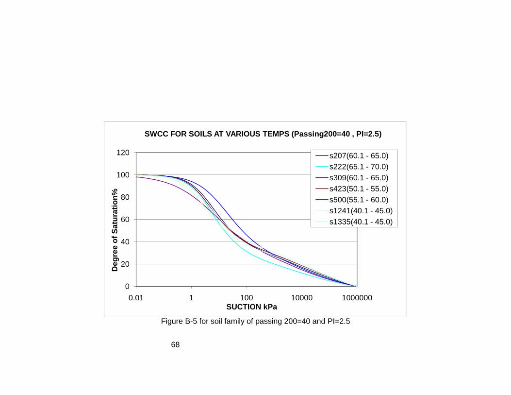
68

Figure B-5 for soil family of passing 200=40 and PI=2.5

0

20

40

60

80

100

120

0.01 1 100 10000 1000000

Deg

ree

of

Sat

ura

tio

n%

SUCTION kPa

SWCC FOR SOILS AT VARIOUS TEMPS (Passing200=40 , PI=2.5)

s207(60.1 - 65.0)s222(65.1 - 70.0)s309(60.1 - 65.0)s423(50.1 - 55.0)s500(55.1 - 60.0)s1241(40.1 - 45.0)s1335(40.1 - 45.0)

69

Figure B-6 SWCC for soil family of passing 200=40 and PI=3.5

0

20

40

60

80

100

120

0.01 1 100 10000 1000000

Deg

ree

of

Sat

ura

tio

n%

SUCTION kPa

SWCC FOR SOILS AT VARIOUS TEMPS (Passing200=40 , PI=3.5)

s28(55.1 - 60.0)s29(55.1 - 60.0)s66(60.1 - 65.0)s1688(55.1 - 60.0)s4699(55.1 - 60.0)s4730(40.1 - 45.0)s4731(32.0 - 40.0)s4737(40.1 - 45.0)s4738(32.0 - 40.0)s5347(55.1 - 60.0)s3398(40.1 - 45.0)s6328(55.1 - 60.0)s6653(60.1 - 65.0)s6659(55.1 - 60.0)

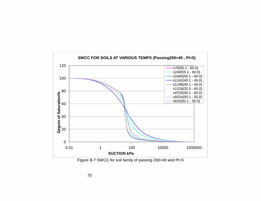
70

Figure B-7 SWCC for soil family of passing 200=40 and PI=5

0

20

40

60

80

100

120

0.01 1 100 10000 1000000

Deg

ree

of

Sat

ura

tio

n%

SUCTION kPa

SWCC FOR SOILS AT VARIOUS TEMPS (Passing200=40 , PI=5)

s76(55.1 - 60.0)s240(55.1 - 60.0)s1683(55.1 - 60.0)s1162(40.1 - 45.0)s1198(40.1 - 45.0)s1318(32.0 - 40.0)s4703(55.1 - 60.0)s5024(50.1 - 55.0)s620(50.1 - 55.0)

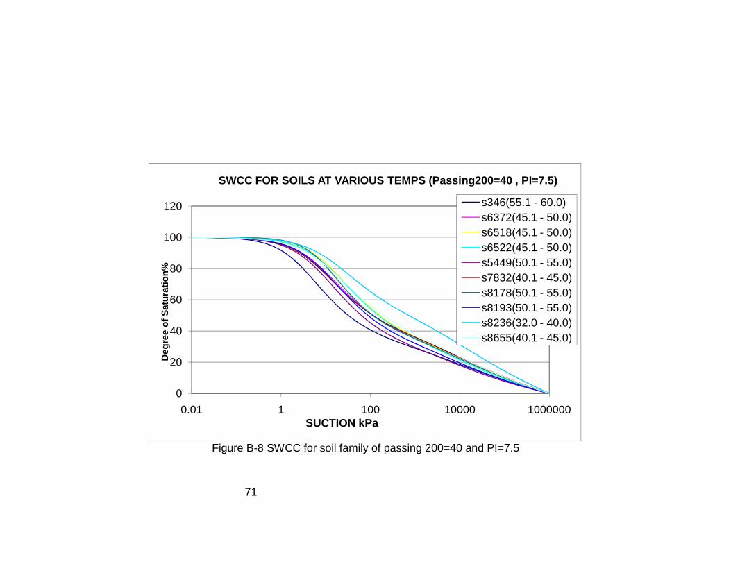
71

Figure B-8 SWCC for soil family of passing 200=40 and PI=7.5

0

20

40

60

80

100

120

0.01 1 100 10000 1000000

Deg

ree

of

Sat

ura

tio

n%

SUCTION kPa

SWCC FOR SOILS AT VARIOUS TEMPS (Passing200=40 , PI=7.5)

s346(55.1 - 60.0)s6372(45.1 - 50.0)s6518(45.1 - 50.0)s6522(45.1 - 50.0)s5449(50.1 - 55.0)s7832(40.1 - 45.0)s8178(50.1 - 55.0)s8193(50.1 - 55.0)s8236(32.0 - 40.0)s8655(40.1 - 45.0)

Figure B-9 SWCC for soil family of passing 200=50 and PI=2.5

0

20

40

60

80

100

120

0.01 1 100 10000 1000000

Deg

ree

of

Sat

ura

tio

n%

Suction kPa

SWCC FOR SOILS AT VARIOUS TEMPS (Passing200=50 , PI=2.5)

s5251(45.1 - 50.0)

s542(45.1 - 50.0)

s6352(40.1 - 45.0)

s6355(40.1 - 45.0)

s1888(40.1 - 45.0)

s5856(50.1 - 55.0)

Figure B-10 SWCC for soil family of passing 200=50 and PI=5

0

20

40

60

80

100

120

0.01 0.1 1 10 100 1000 10000 100000 1000000Deg

ree

of

Sat

ura

tio

n%

Suction kPa

SWCC FOR SOILS AT VARIOUS TEMPS (Passing200=50 , PI=5)

s5049-E 50.1 - 55.0s4032-C 40.1 - 45.0s9122-B 32.0 - 40.0

FigureB-11 SWCC for soil family of passing 200=50 and PI=7.5

0

20

40

60

80

100

120

0.01 0.1 1 10 100 1000 10000 100000 1000000

Deg

ree

of

Sat

ura

tio

n%

Suction kPa

SWCC FOR SOILS AT VARIOUS TEMPS (Passing200=50 , PI=7.5)

s381-E 50.1 - 55.0s493-F 55.1 - 60.0s5338-E 50.1 - 55.0s6504-C 40.1 - 45.0s6177-E 50.1 - 55.0s4029-B 32.0 - 40.0s8622-D 45.1 - 50.0

Figure B-12 for soil family of passing 200=60 and PI=0

0

20

40

60

80

100

120

0.01 0.1 1 10 100 1000 10000 100000 1000000

Deg

ree

of

Sat

ura

tio

n%

Suction kPa

SWCC FOR SOILS AT VARIOUS TEMPERATURES(Passing200=60 , PI=0)

s6527-D 45.1 - 50.0s7173-G 60.1 - 65.0s7174-G 60.1 - 65.0s7306-H 65.1 - 70.0s1200-A < 32.0s3113-C 40.1 - 45.0s4169-B 32.0 - 40.0s4324-C 40.1 - 45.0s7105-F 55.1 - 60.0s7132-E 50.1 - 55.0

Figure B-13 SWCC for soil family of passing 200=60 and PI=5

0

20

40

60

80

100

120

0.01 1 100 10000 1000000

Deg

ree

of

Sat

ura

tio

n%

Suction kPa

SWCC FOR SOILS AT VARIOUS TEMPERATURES(Passing200=60 , PI=5)

s85-F 55.1 - 60.0s1200-A < 32.0s3299-D 45.1 - 50.0s4169-B 32.0 - 40.0

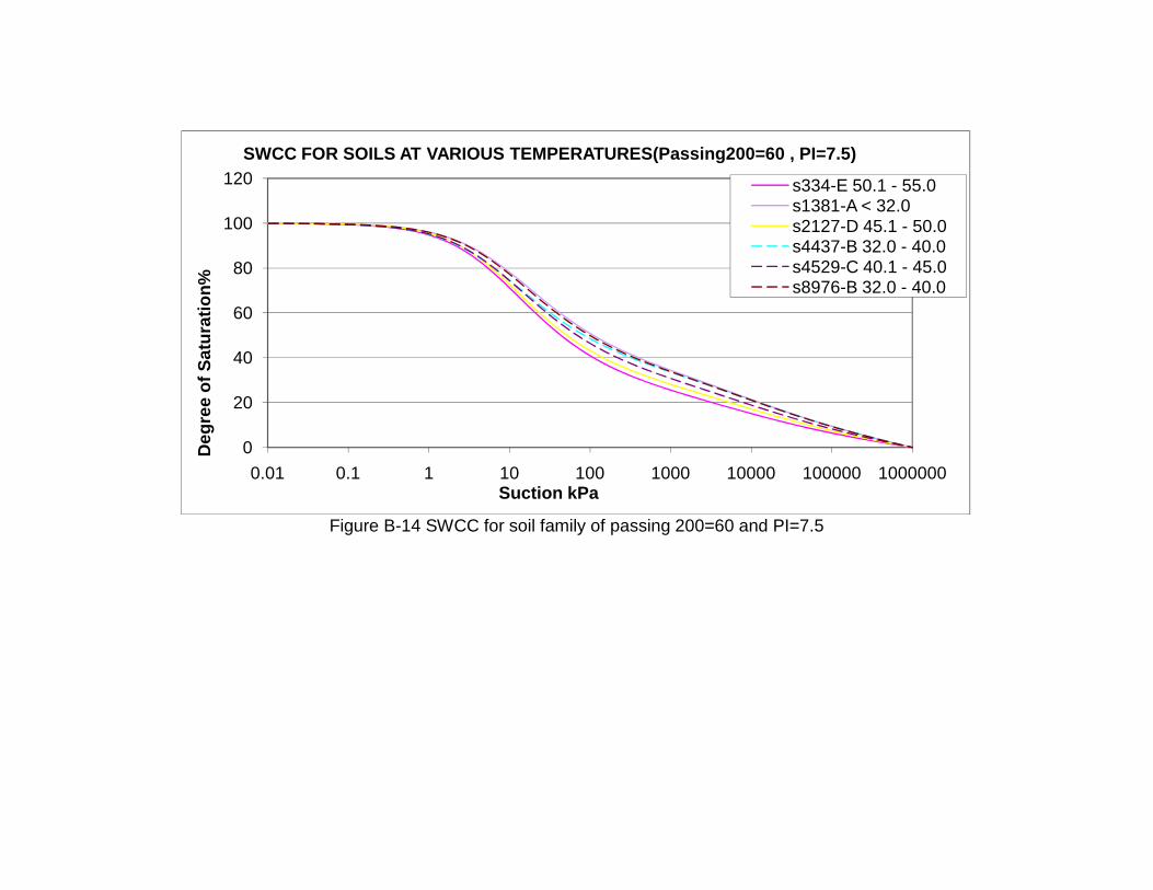
Figure B-14 SWCC for soil family of passing 200=60 and PI=7.5

0

20

40

60

80

100

120

0.01 0.1 1 10 100 1000 10000 100000 1000000

Deg

ree

of

Sat

ura

tio

n%

Suction kPa

SWCC FOR SOILS AT VARIOUS TEMPERATURES(Passing200=60 , PI=7.5)

s334-E 50.1 - 55.0s1381-A < 32.0s2127-D 45.1 - 50.0s4437-B 32.0 - 40.0s4529-C 40.1 - 45.0s8976-B 32.0 - 40.0

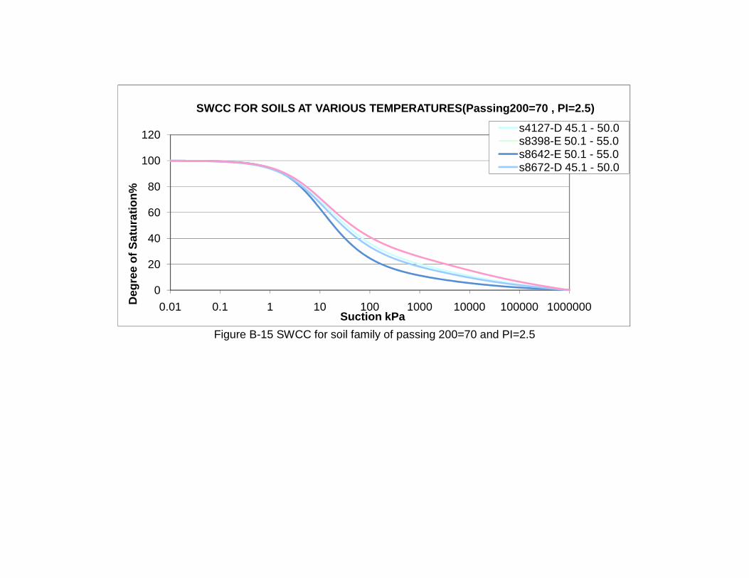
Figure B-15 SWCC for soil family of passing 200=70 and PI=2.5

0

20

40

60

80

100

120

0.01 0.1 1 10 100 1000 10000 100000 1000000Deg

ree

of

Sat

ura

tio

n%

Suction kPa

SWCC FOR SOILS AT VARIOUS TEMPERATURES(Passing200=70 , PI=2.5)

s4127-D 45.1 - 50.0s8398-E 50.1 - 55.0s8642-E 50.1 - 55.0s8672-D 45.1 - 50.0

Figure B-16 SWCC for soil family of passing 200=70 and PI=5

0

20

40

60

80

100

120

0.01 0.1 1 10 100 1000 10000 100000 1000000

Deg

ree

of

Sat

ura

tio

n%

Suction KPa

SWCC FOR SOILS AT VARIOUS TEMPERATURES(Passing200=70 , PI=5)

s260-G 60.1 - 65.0s262-G 60.1 - 65.0s4812-C 40.1 - 45.0s5427-E 50.1 - 55.0

Figure B-17 SWCC for soil family of passing 200=70 and PI=7.5

0

20

40

60

80

100

120

0.01 0.1 1 10 100 1000 10000 100000 1000000

Deg

ree

of

Sat

ura

tio

n%

Suction KPa

SWCC FOR SOILS AT VARIOUS TEMPERATURES(Passing200=70 , PI=7.5)

s2796-H 65.1 - 70.0s8797-D 45.1 - 50.0s239-F 55.1 - 60.0s5363-D 45.1 - 50.0s7800-E 50.1 - 55.0s4252-C 40.1 - 45.0

Figure B-18 SWCC for soil family of passing 200=70 and PI=9-10

0

20

40

60

80

100

120

0.01 0.1 1 10 100 1000 10000 100000 1000000

Deg

ree

of

Sat

ura

tio

n %

Suction KPa

SWCC FOR SOILS AT VARIOUS TEMPERATURES(Passing200=70 , PI=9-10)

s2316-E 50.1 - 55.0s6065-E 50.1 - 55.0s3633-C 40.1 - 45.0s4764-C 40.1 - 45.0s4766-B 32.0 - 40.0s5192-D 45.1 - 50.0s3962-H 65.1 - 70.0s6603-D 45.1 - 50.0

Figure B-19 SWCC for soil family of passing 200=80 and PI=5

0

20

40

60

80

100

120

0.01 0.1 1 10 100 1000 10000 100000 1000000

Deg

ree

of

Sat

ura

tio

n%

Suction KPa

SWCC FOR SOILS AT VARIOUS TEMPERATURES(Passing200=80 , PI=5)

s6425-E 50.1 - 55.0s2803-H 65.1 - 70.0s3829-G 60.1 - 65.0s6545-D 45.1 - 50.0s6721-G 60.1 - 65.0

Figure B-20 SWCC for soil family of passing 200=80 and PI=7.5

0

20

40

60

80

100

120

0.01 0.1 1 10 100 1000 10000 100000 1000000

Deg

ree

of

Sat

ura

tio

n %

Suction KPa

SWCC FOR SOILS AT VARIOUS TEMPERATURES(Passing200=80 , PI=7.5)

s5290-F 55.1 - 60.0s6398-E 50.1 - 55.0s2642-E 50.1 - 55.0s2657-E 50.1 - 55.0s7816-B 32.0 - 40.0s7835-C 40.1 - 45.0s4147-D 45.1 - 50.0s7968-E 50.1 - 55.0s7989-E 50.1 - 55.0

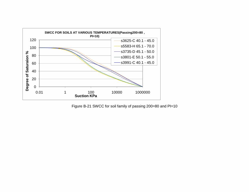
Figure B-21 SWCC for soil family of passing 200=80 and PI=10

0

20

40

60

80

100

120

0.01 1 100 10000 1000000

Deg

ree

of

Sat

ura

ion

%

Suction KPa

SWCC FOR SOILS AT VARIOUS TEMPERATURES(Passing200=80 , PI=10)

s3625-C 40.1 - 45.0

s5583-H 65.1 - 70.0

s3735-D 45.1 - 50.0

s3801-E 50.1 - 55.0

s3991-C 40.1 - 45.0

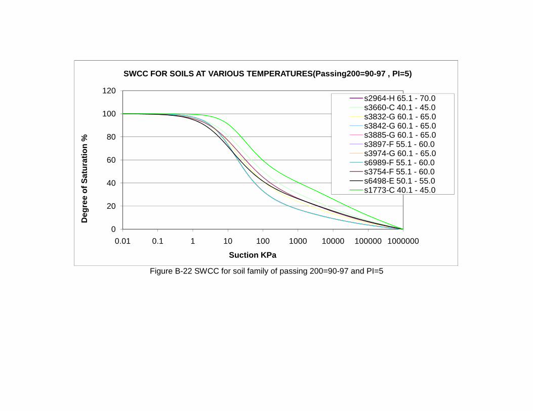
Figure B-22 SWCC for soil family of passing 200=90-97 and PI=5

0

20

40

60

80

100

120

0.01 0.1 1 10 100 1000 10000 100000 1000000

Deg

ree

of

Sat

ura

tio

n %

Suction KPa

SWCC FOR SOILS AT VARIOUS TEMPERATURES(Passing200=90-97 , PI=5)

s2964-H 65.1 - 70.0s3660-C 40.1 - 45.0s3832-G 60.1 - 65.0s3842-G 60.1 - 65.0s3885-G 60.1 - 65.0s3897-F 55.1 - 60.0s3974-G 60.1 - 65.0s6989-F 55.1 - 60.0s3754-F 55.1 - 60.0s6498-E 50.1 - 55.0s1773-C 40.1 - 45.0

Figure B-23 SWCC for soil family of passing 200=90-97 and PI=7.5

0

20

40

60

80

100

120

0.01 0.1 1 10 100 1000 10000 100000 1000000

Deg

ree

of

Sat

ura

ion

%

Suction KPa

SWCC FOR SOILS AT VARIOUS TEMPERATURES(Passing200=90-97 , PI=7.5)

s2745-E 50.1 - 55.0s2746-F 55.1 - 60.0s1883-C 40.1 - 45.0s2379-E 50.1 - 55.0s236-G 60.1 - 65.0s2959-H 65.1 - 70.0s3000-G 60.1 - 65.0s2106-D 45.1 - 50.0s3891-F 55.1 - 60.0

Figure B-24 SWCC for soil family of passing 200=90-97 and PI=10

0

20

40

60

80

100

120

0.01 0.1 1 10 100 1000 10000 100000 1000000

Deg

ree

of

Sat

ura

tio

n %

Suction KPa

SWCC FOR SOILS AT VARIOUS TEMPERATURES(Passing200=90-97 , PI=10)

s1717-D 45.1 - 50.0

s245-G 60.1 - 65.0

s1738-D 45.1 - 50.0

s1818-D 45.1 - 50.0

s2272-E 50.1 - 55.0

s4872-E 50.1 - 55.0

s3738-E 50.1 - 55.0

s1705-C 40.1 - 45.0

s1706-D 45.1 - 50.0

Figure B-25 SWCC for soil family of passing 200=90-97 and PI=12.5

0

20

40

60

80

100

120

0.01 0.1 1 10 100 1000 10000 100000 1000000

Deg

ree

of

Sat

ura

tio

n %

Suction KPa

SWCC FOR SOILS AT VARIOUS TEMPERATURES(Passing200=90-97 , PI=12.5)

s4892-D 45.1 - 50.0s2133-D 45.1 - 50.0s2221-C 40.1 - 45.0s2236-D 45.1 - 50.0s2264-E 50.1 - 55.0

Figure B-26 SWCC for soil family of passing 200=90-97 and PI=15

0

20

40

60

80

100

120

0.01 0.1 1 10 100 1000 10000 100000 1000000

Deg

ree

of

Sat

ura

tio

n%

Suction KPa

SWCC FOR SOILS AT VARIOUS TEMPERATURES(Passing200=90-97 , PI=15)

s9468-0

s4021-D 45.1 -50.0s3514-C 40.1 -45.0