evaluation of retention basins and soil amendments …
TRANSCRIPT

1
EVALUATION OF RETENTION BASINS AND SOIL AMENDMENTS TO IMPROVE STORMWATER MANAGEMENT IN FLORIDA
By
EBAN ZACHARY BEAN
A DISSERTATION PRESENTED TO THE GRADUATE SCHOOL OF THE UNIVERSITY OF FLORIDA IN PARTIAL FULFILLMENT
OF THE REQUIREMENTS FOR THE DEGREE OF DOCTOR OF PHILOSOPHY
UNIVERSITY OF FLORIDA
2010

2
© 2010 Eban Zachary Bean

3
I dedicate this work to my wife who has provided unwavering support.

4
ACKNOWLEDGMENTS
For challenging me intellectually and supporting me, I thank my advisor, Dr.
Michael Dukes. Dr. Dukes has encouraged me in my research and reiterated its
importance. His professionalism and example has been an inspiration to me. For
providing guidance and support as members of my Ph.D. committee, I also thank Drs.
John Sansalone, James Heaney, Mark Clark, and Pierce Jones. I sincerely appreciate
the time and energy they have invested in guiding my research and assisting in my
professional development.
I am extremely thankful for the assistance and friendship of Christian Guzman,
who worked tirelessly under the most trying conditions. I also would like to thank the
staff within the Agricultural and Biological Engineering department, specifically: Jimmy
Rummel, Billy Duckworth, Dan Burch, Orlando Lanni, Hannah O’Malley and Steve
Feagle. This research would not have been completed without each one of them. In
particular, Paul Lane went above and beyond to assist me with completing my project.
For sample analysis and advising on sample submission I thank Nancy Wilkinson,
Bill D’Angelo and Lamar Moon at the Analytical Research Laboratory. I would also like
to thank Eric Livingston and the Florida Department of Environmental Protection for
funding this research. Numerous officials from Suwannee and Northwest Florida Water
Management Districts, Leon, Alachua, and Marion Counties, the City of Tallahassee,
and the Florida Department of Transportation assisted specifically with supplying
access and documentation for basins studied. Finally for encouragement, support,
friendship, and great discussion, I thank Hal Knowles and Brent Philpot.

5
TABLE OF CONTENTS page
ACKNOWLEDGMENTS .................................................................................................. 4
LIST OF TABLES ............................................................................................................ 9
LIST OF FIGURES ........................................................................................................ 15
ABSTRACT ................................................................................................................... 19
CHAPTER
1 INTRODUCTION AND RESEARCH OBJECTIVES ................................................ 21
Introduction ............................................................................................................. 21 Federal Regulations ......................................................................................... 21 Florida Regulations .......................................................................................... 23
Reducing stormwater production ............................................................... 25 Low-Impact development ........................................................................... 26
Soil Compaction ...................................................................................................... 27 Compost ........................................................................................................... 29 Fly Ash ............................................................................................................. 31
Objectives ............................................................................................................... 36
2 EVALUATION OF RETENTION BASIN PERFORMANCE IN FLORIDA ................ 39
Introduction ............................................................................................................. 39 Stormwater Control .......................................................................................... 39 Retention Basins .............................................................................................. 39 Design and Permitting ...................................................................................... 41
Materials & Methods ............................................................................................... 45 Infiltration Basin Selection ................................................................................ 45
Basin documentation ................................................................................. 45 Basin inspection ......................................................................................... 47 Permission ................................................................................................. 47 Selected basins .......................................................................................... 47
Infiltration Rate Measurements ......................................................................... 47 Soil Sample Collection ..................................................................................... 50
Bulk density and volumetric water content ................................................. 51 Soil organic matter by loss on ignition ........................................................ 51 Soil texture by hydrometer ......................................................................... 52
Monitoring ......................................................................................................... 53 Data Analysis ................................................................................................... 54 Modeling ........................................................................................................... 55
Results .................................................................................................................... 58 Soil Texture ...................................................................................................... 58

6
Infiltration Rates ............................................................................................... 59 Soil Organic Matter ........................................................................................... 59 Bulk Density ..................................................................................................... 60 Modeling ........................................................................................................... 60
Analysis .................................................................................................................. 61 Monitored vs. DRI ............................................................................................. 61 DRI and Monitored vs. Design .......................................................................... 62 DRI Infiltration Rates ........................................................................................ 62 Effects of Age ................................................................................................... 63 Vegetation ........................................................................................................ 65 Hydraulic Conductivity Models ......................................................................... 68
Summary and Conclusions ..................................................................................... 71
3 SOIL AMEMDMENTS FOR COMPACTED SOIL MITIGATION I: HYDROLOGY ... 92
Introduction ............................................................................................................. 92 Materials and Methods............................................................................................ 93
Non-compacted Phase ..................................................................................... 95 Compaction Phase ........................................................................................... 98 Amendment Phase ......................................................................................... 101
Results and Discussion......................................................................................... 104 Non-compacted Phase ................................................................................... 105 Compacted Phase .......................................................................................... 107
Bulk densities ........................................................................................... 107 Infiltration rates ........................................................................................ 108 Rainfall and runoff data ............................................................................ 109 Runoff coefficients and curve numbers .................................................... 110 Cone index profiles .................................................................................. 111
Amendment Phase ......................................................................................... 112 Bulk densities ........................................................................................... 112 Cone index profiles .................................................................................. 113 Infiltration rates ........................................................................................ 114 Runoff coefficients ................................................................................... 116 Curve numbers ........................................................................................ 117
Conclusions .......................................................................................................... 119
4 SOIL AMEMDMENTS FOR COMPACTED SOIL MITIGATION II: WATER QUALITY .............................................................................................................. 147
Introduction ........................................................................................................... 147 Methods and Materials.......................................................................................... 148
Soils and Amendments................................................................................... 148 Column Study ................................................................................................. 149 Lysimeter Study .............................................................................................. 150 Sampling and Analysis Methodology .............................................................. 151 Data Analysis ................................................................................................. 152
Results and Discussion......................................................................................... 153

7
Column Study ................................................................................................. 153 Nitrogen ................................................................................................... 153 Ortho-phosphorus .................................................................................... 155 Metals ...................................................................................................... 155
Lysimeter Results ........................................................................................... 156 Rainfall Water Quality .............................................................................. 156 NO2+3-N .................................................................................................... 157 NH4-N ....................................................................................................... 158 TKN .......................................................................................................... 159 OP ............................................................................................................ 161 pH ............................................................................................................ 162
Lysimeter Runoff Loadings ............................................................................. 163 Nitrogen ................................................................................................... 163 Ortho-phosphorus .................................................................................... 164
Lysimeter Leachate Loadings ......................................................................... 165 Nitrogen ................................................................................................... 165 Ortho-phosphorus .................................................................................... 166
Conclusions .......................................................................................................... 167
5 CONCLUSIONS ................................................................................................... 179
Retention Basins ................................................................................................... 179 Performance Conclusions .............................................................................. 179 Recommendations and Future Research ....................................................... 181
Soil Amendments .................................................................................................. 182 Hydrologic Conclusions .................................................................................. 182
Amendment phase ................................................................................... 182 Applications .............................................................................................. 183
Water Quality Conclusions ............................................................................. 184 Recommendations and Future Research ....................................................... 185
APPENDIX
A RETENTION BASIN DATA ................................................................................... 188
B SOIL MOISTURE AND CONE PENETROMETER DATA ..................................... 195
Soil Moisture ......................................................................................................... 195 Time Domain Reflectometer ........................................................................... 195 Volumetric Water Content .............................................................................. 195
Soil Strength ......................................................................................................... 196
C MONITORING DATA ............................................................................................ 203
D ADDITIONAL HYDROLOGIC AND SOILS DATA ................................................. 210
E LYSIMETER WATER QUALITY RESULTS .......................................................... 245

8
F ADDITIONAL COLUMN STUDY WATER QUALITY DATA .................................. 277
Leachate Column Results ..................................................................................... 277 Total Phosphorus (TP) ................................................................................... 277 Potassium (K) ................................................................................................. 277 Sodium (Na) ................................................................................................... 277 Magnesium (Mg) ............................................................................................ 278 Calcium (Ca) .................................................................................................. 278 Aluminum (Al) ................................................................................................. 278 Iron (Fe) .......................................................................................................... 278 Manganese (Mn) ............................................................................................ 279 Zinc (Zn) ......................................................................................................... 279 Copper (Cu) .................................................................................................... 279 Boron (B) ........................................................................................................ 280 Nickel (Ni), Cadmium (Cd), and Lead (Pb) ..................................................... 280 Summary ........................................................................................................ 280
Fly Ash TCLP ........................................................................................................ 281
LIST OF REFERENCES ............................................................................................. 290
BIOGRAPHICAL SKETCH .......................................................................................... 302

9
LIST OF TABLES
Table page 2-1 Pedotransfer function models ............................................................................. 75
2-2 Pedotransfer model definitions for models in Table 2-1. ..................................... 77
2-3 Number of soil sample textures between land uses. .......................................... 77
2-4 Distribution of total and monitored number of basins .......................................... 78
2-5 Design, double ring infiltrometer, and monitored infiltration rates ....................... 78
2-6 Soil organic matter percentages for all sites by soil texture classification. .......... 79
2-7 Summary of model variable values from fitting double ring infiltrometer infiltration rate data. ............................................................................................ 79
2-8 Student t-statistic and p-values for infiltration rate comparisons for monitored basins. ................................................................................................................ 80
2-9 Summary of measured infiltration rate analysis for all basins. ............................ 80
2-10 Regression values for log ratio against log of basin age by Department of Transportation basins. ........................................................................................ 81
2-11 Regression values for log ratio against log of basin age residential basins. ....... 81
3-1 Summary of properties for soils and amendments included in this study. ........ 122
3-2 Non-compacted bulk densities.......................................................................... 122
3-3 Non-compacted infiltration rates ....................................................................... 122
3-4 Pearson correlation coefficients and for non-compacted bulk density and infiltration rate. .................................................................................................. 122
3-5 Pearson correlation coefficients and for cone indices with bulk densities and infiltration rates. ................................................................................................ 123
3-6 Arredondo bulk densities and mean bulk density increase for each compaction iteration. ........................................................................................ 123
3-7 Orangeburg bulk densities and mean bulk density increase from each compaction iteration. ........................................................................................ 124
3-8 Compacted bulk densities and percent of growth limiting bulk densities .......... 124

10
3-9 Summary of compacted infiltration rates. ......................................................... 124
3-10 Scaling Factors for compacted phase .............................................................. 125
3-11 Rainfall event dates, depth, and effective rainfall depths. ................................. 125
3-12 Summary of compaction phase runoff coefficients for each soil. ...................... 126
3-13 Summary of compacted regressed curve numbers. ......................................... 126
3-14 Mean bulk densities (g/cm3) for each soil for each treatment. .......................... 126
3-15 ANOVA for amended phase bulk density results. ............................................. 127
3-16 Multiple linear regression results of amended bulk densities. ........................... 127
3-17 ANOVA for amended phase log of infiltration rates results. .............................. 127
3-18 Summary of log of infiltration rate mean. .......................................................... 128
3-19 Regression results of log-transformed amended infiltration rates. .................... 128
3-20 Geometric means and standard deviations of amended infiltration rates ......... 129
3-21 Summary of depths from the surface of significant difference in cone index .... 129
3-22 Amended phase rainfall events and depths which runoff was measured. ........ 130
3-23 Summary of amendment phase Arredondo runoff coefficients. ........................ 130
3-24 Summary of amendment phase Orangeburg treatment runoff coefficients. ..... 131
3-25 Arredondo curve number regression against inverse of rainfall depth. ............. 131
3-26 Orangeburg curve number regression against inverse of rainfall depth. .......... 131
3-27 Summarized mean curve numbers for amended Arredondo treatments. ......... 132
3-28 Summarized mean curve numbers for amended Orangeburg treatments. ....... 132
3-29 Hypothetical runoff for Gainesville, FL for open areas treated with tillage ........ 132
4-1 Summary of properties for soils and amendments included in this study. ........ 169
4-2 Practical quantitation limits, method detection limit, and column water matrix concentrations for analytes. .............................................................................. 169
4-3 p-values for comparing soil and amendment mixture to soil column leached concentrations. ................................................................................................. 170

11
4-4 Summary of rain event types, depths, and water quality characteristics .......... 171
4-5 Arredondo median runoff pHs and concentrations. .......................................... 171
4-6 Orangeburg runoff median pHs and concentrations. ........................................ 172
4-7 Arredondo leachate median pHs and concentrations. ...................................... 172
4-8 Orangeburg leachate median pHs and concentrations. .................................... 172
4-9 Mean Arredondo total runoff loadings ............................................................... 173
4-10 Mean Orangeburg total runoff loadings ............................................................ 173
4-12 Mean Orangeburg total leachate loadings ........................................................ 174
A-1 Comparison of stormwater retention design criteria for Water Management Districts in Florida. ............................................................................................ 188
A-2 Basin number, county location, land use, age, and design infiltration rates. .... 190
A-3 Soil textures for each basin test location and corresponding median basin texture. ............................................................................................................. 191
A-4 Soil organic matter percentages by percent weight from loss on ignition. ........ 192
A-5 Bulk density measurements from each basin location. ..................................... 193
A-6 Measured double ring infiltrometer infiltration rates for each basin test location. ............................................................................................................ 194
B-1 Volumetric water content by TDR attempts and successes for each basin. ..... 198
B-2 Gravimetric volumetric water content measurements from each basin location. ............................................................................................................ 199
B-3 Summary table of attempts, complete, truncated profile measurements, and average depth of maximum reading for each basin. ......................................... 200
B-4 Correlation and probability values between cone penetrometer measurements at 2.5 cm increments and measured infiltration rates in basins for full profiles. .................................................................................................. 201
C-1 Summary of drawdown events for monitoring in basin 4. ................................. 203
C-2 Summary of drawdown events for monitoring in basin 5 .................................. 205
C-3 Summary of drawdown events for monitoring in basin 6 .................................. 206

12
C-4 Summary of drawdown events for monitoring in basin 13 ................................ 206
C-5 Summary of drawdown events for monitoring in basin 18. ............................... 207
C-6 Summary of drawdown events for monitoring in basin 21 ................................ 208
C-7 Summary of drawdown events for monitoring in basin 25 ................................ 208
C-8 Summary of drawdown events for monitoring in basin 30. ............................... 209
D-1 Distribution uniformities and uniformity coefficients for natural and simulated events ............................................................................................................... 210
D-2 Non-compacted bulk densities.......................................................................... 211
D-3 Non-compacted infiltration rates ....................................................................... 212
D-4 Non-compacted summary of cone indices profiles. .......................................... 213
D-5 Student t-test results for cone index values ...................................................... 214
D-6 Compacted bulk densities. ............................................................................... 215
D-7 Compacted infiltration rates. ............................................................................. 216
D-8 Runoff coefficients for each Arredondo lysimeter ............................................. 217
D-9 Runoff coefficients for each Orangeburg lysimeter ........................................... 218
D-10 Calculated and regressed curve numbers from compacted Arredondo lysimeters. ........................................................................................................ 219
D-11 Calculated and regressed curve numbers from compacted Orangeburg lysimeters. ........................................................................................................ 220
D-12 Amendment phase Arredondo bulk densities. .................................................. 221
D-13 Amendment phase Orangeburg bulk densities. ................................................ 222
D-14 Amendment phase Arredondo infiltration rates. ............................................... 223
D-15 Amendment phase Orangeburg infiltration rates. ............................................. 224
D-16 Summary of Arredondo cone index profiles indicating significant difference between control treatments .............................................................................. 225
D-17 Summary of Orangeburg cone index profiles indicating significant difference between control treatments .............................................................................. 226

13
D-18 Arredondo amended runoff coefficients. ........................................................... 227
D-18 Arredondo amended runoff coefficients. ........................................................... 228
D-19 Orangeburg amended runoff coefficients. ........................................................ 229
D-20 Calculated curve numbers for amended Arredondo lysimeters. ....................... 231
D-21 Calculated curve numbers from amended Orangeburg soils. ........................... 233
D-22 Summary of Arredondo calculated curve numbers regressed against inverse rainfall depths. .................................................................................................. 235
D-23 Summary of Orangeburg calculated curve numbers regressed against inverse rainfall depths. ...................................................................................... 236
E-1 Type, date, depth and water quality results for 16 rainfall events on lysimeters. ........................................................................................................ 245
E-2 Concentrations from homogenous column samples. ........................................ 246
E-3 Column leachate concentrations from Arredondo and compost mixtures. ........ 247
E-4 Column leachate concentrations from Arredondo and fly ash mixtures. ........... 247
E-5 Column leachate concentrations from Orangeburg and compost mixtures. ..... 248
E-6 Column leachate concentrations from Orangeburg and fly ash mixtures. ........ 248
E-7 Arredondo NH4-N concentrations (mg/l) ........................................................... 249
E-8 Orangeburg NH4-N concentrations (mg/l). ........................................................ 251
E-9 Arredondo NO2+3-N concentrations (mg/l) ........................................................ 253
E-10 Orangeburg NO2+3-N concentrations (mg/l) ...................................................... 255
E-11 Arredondo TKN concentrations (mg/l) .............................................................. 257
E-12 Orangeburg TKN concentrations (mg/l) ............................................................ 259
E-13 Arredondo OP concentrations (ug/l). ................................................................ 261
E-14 Orangeburg OP sample concentrations (ug/l). ................................................. 262
E-15 Arredondo pH ................................................................................................... 263
E-16 Orangeburg ph. ................................................................................................ 265

14
F-1 Practical quantitation limits, minimum detection limits and applied water matrix concentrations. ...................................................................................... 281
F-2 Toxicity characteristic leaching protocol results for fly ash sample, with corresponding lab practical quantitation level, minimum detection level, and toxicity limits. .................................................................................................... 282

15
LIST OF FIGURES
Figure page 2-1 Various testing location orientations based on basin geometry. ......................... 82
2-2 Infiltration rate measurement using double-ring infiltrometer with Mariotte siphon. ................................................................................................................ 82
2-3 Infiltration rate measurement data from six sites at one infiltration basin ........... 83
2-4 Monitoring installation with water level recorder housing and rain gauges ......... 83
2-5 Frequency and cumulative distribution of double ring infiltrometer infiltration rates ................................................................................................................... 84
2-6 Frequency and cumulative distribution of log transformed double ring infiltrometer infiltration rates................................................................................ 84
2-7 Modeled Ks versus measured Ks for models. .................................................... 85
2-8 Regression of double ring infiltrometer (DRI) and monitored infiltration rates .... 88
2-9 Distribution of t-statistics log of infiltration rate ratios .......................................... 88
2-10 Example of size and diversity of vegetation in basin 9. ...................................... 89
2-11 Limited vegetation size and diversity in basin 39. ............................................... 90
2-12 Photo of basin 8 during double ring infiltrometer testing. .................................... 91
3-1 Centerline, cross-sectional diagram of a lysimeter from the left side. ............... 133
3-2 A) Well screen installed in the bottom of a lysimeter prior to filling. B) Measurement of drainage layer depth after filling. ............................................ 133
3-3 A) Filter fabric installed over drainage layer. B) Screening of Orangeburg soil during lysimeter filling. ...................................................................................... 133
3-4 A) Moving filled lysimeter via forklift. B) Lysimeters placed in their respective locations. .......................................................................................................... 134
3-5 Soil moisture sensor diagram. .......................................................................... 134
3-6 Soil compaction using tamper and slide weight. ............................................... 135
3-7 Compaction during final iteration using modified tamper. ................................. 135

16
3-8 Schematic of lysimeter layout and rainfall simulator. Soil types are identified for each lysimeter as A (Arredondo) or O (Orangeburg). .................................. 136
3-9 Non-compacted bulk density values. ................................................................ 136
3-10 Non-compacted infiltration rates ....................................................................... 137
3-11 Maximum, mean, median, and minimum value cone penetrometer profiles ..... 137
3-12 Bulk densities following compaction iterations. ................................................. 138
3-13 Infiltration rates versus bulk densities for non-compacted and compacted lysimeters. ........................................................................................................ 139
3-14 Comparison of median non-compacted and control cone index profiles. ......... 140
3-15 Median Arredondo null amended cone index profiles. ...................................... 141
3-16 Median Arredondo compost amended cone index profiles. .............................. 142
3-17 Median Arredondo fly ash amended cone index profiles. ................................. 143
3-18 Median Orangeburg null amended cone index profiles. ................................... 144
3-19 Median Orangeburg compost amended cone index profiles. ........................... 145
3-20 Median Orangeburg Fly Ash amended cone index profiles. ........................... 146
4-1 NH4-N water matrix and column leachate concentrations................................. 174
4-2 NO2+3-N water matrix and column leachate concentrations .............................. 175
4-3 TKN water matrix and column leachate concentrations .................................... 175
4-4 ON water matrix and column leachate concentrations ..................................... 176
4-5 TN water matrix and column leachate concentrations ...................................... 176
4-6 OP water matrix and column leachate concentrations ...................................... 177
4-7 pH of water matrix and column leachate .......................................................... 177
4-8 Total nitrogen median results from each of the four soil-amendment combinations .................................................................................................... 178
B-1 Average TDR VWC readings vs. Gravimetric VWC for each location tested. ... 202
D-1 Results from standard proctor density method soil samples. ........................... 237
17
D-2 Curve number regression for Arredondo Null incorporation at 0 cm. ................ 237
D-3 Curve number regression for Arredondo Null incorporation at 10 cm. .............. 238
D-4 Curve number regression for Arredondo Null incorporation at 20 cm. .............. 238
D-5 Curve number regression for Arredondo Fly Ash incorporation at 10 cm. ........ 239
D-6 Curve number regression for Arredondo Fly Ash incorporation at 20 cm. ........ 239
D-7 Curve number regression for Arredondo Compost incorporation at 10 cm. ...... 240
D-8 Curve number regression for Arredondo Compost incorporation at 20 cm. ...... 240
D-9 Curve number regression for Orangeburg Null incorporation at 0 cm. ............. 241
D-10 Curve number regression for Orangeburg Null incorporation at 10 cm. ........... 241
D-11 Curve number regression for Orangeburg Null incorporation at 20 cm. ........... 242
D-12 Curve number regression for Orangeburg Fly Ash incorporation at 10 cm. ...... 242
D-13 Curve number regression for Orangeburg Fly Ash incorporation at 20 cm. ...... 243
D-14 Curve number regression for Orangeburg Compost incorporation at 10 cm. ... 243
D-15 Curve number regression for Orangeburg Compost incorporation at 20 cm. ... 244
E-1 Arredondo mean runoff NH4-N concentrations ................................................. 267
E-2 Orangeburg mean runoff NH4-N concentrations. .............................................. 267
E-3 Arredondo mean leachate NH4-N concentrations ............................................. 268
E-4 Orangeburg mean leachate NH4-N concentrations .......................................... 268
E-5 Arredondo mean runoff NO2+3-N Concentrations ............................................. 269
E-6 Orangeburg mean runoff NO2+3-N concentrations ............................................ 269
E-7 Arredondo mean leachate NO2+3-N concentrations .......................................... 270
E-8 Orangeburg mean leachate NO2+3-N concentrations........................................ 270
E-9 Arredondo mean runoff TKN concentrations .................................................... 271
E-10 Orangeburg mean runoff TKN concentrations .................................................. 271
E-11 Arredondo mean leachate TKN concentrations ................................................ 272

18
E-12 Orangeburg mean leachate TKN concentration ............................................... 272
E-13 Arredondo mean runoff OP concentrations ...................................................... 273
E-14 Orangeburg mean runoff OP concentrations .................................................... 273
E-15 Arredondo mean leachate OP concentrations .................................................. 274
E-16 Orangeburg mean leachate OP concentrations................................................ 274
E-17 Arredondo mean runoff pH ............................................................................... 275
E-18 Arredondo mean leachate pH ............................................................................. 275
E-19 Orangeburg mean runoff pH ............................................................................. 276
E-20 Orangeburg mean leachate pH ........................................................................ 276
F-1 TP column leachate concentrations for soil and amendment mixtures. ............ 283
F-2 K column leachate concentrations for soil and amendment mixtures. .............. 283
F-3 Na column leachate concentrations for soil and amendment mixtures. ............ 284
F-4 Mg column leachate concentrations for soil and amendment mixtures. ........... 284
F-5 Ca column leachate concentrations for soil and amendment mixtures. ............ 285
F-6 Al column leachate concentrations for soil and amendment mixtures. ............. 285
F-7 Fe column leachate concentrations for soil and amendment mixtures. ............ 286
F-8 Mn column leachate concentrations for soil and amendment mixtures. ........... 286
F-9 Zn column leachate concentrations for soil and amendment mixtures. ............ 287
F-10 Cu column leachate concentrations for soil and amendment mixtures. ............ 287
F-11 B column leachate concentrations for soil and amendment mixtures. .............. 288
F-12 Ni column leachate concentrations for soil and amendment mixtures. ............. 288
F-13 Cd column leachate concentrations for soil and amendment mixtures. ............ 289
F-14 Pb column leachate concentrations for soil and amendment mixtures. ............ 289

19
Abstract of Dissertation Presented to the Graduate School of the University of Florida in Partial Fulfillment of the Requirements for the Degree of Doctor of Philosophy
EVALUATION OF RETENTION BASINS AND SOIL AMENDMENTS TO IMPROVE
STORMWATER MANAGEMENT IN FLORIDA
By
Eban Zachary Bean
August 2010
Chair: Michael Dukes Cochair: John Sansalone Major: Agricultural and Biological Engineering
The research presented here addressed two aspects of stormwater prevention.
The first aspect was the elimination of stormwater through retention basins. Infiltration
rates were measured by Double Ring Infiltrometer (DRI) within 40 basins in Alachua,
Leon, and Marion counties. Measured rates were compared to designed rates to
determine whether basins were operating as designed. The 40 basins were equally
divided between residential and Florida Department of Transportation land uses.
Texture analysis was also performed on soil samples taken from each infiltration
location; soil types ranged from sand to sandy clays. Eleven of the 40 basins were also
instrumented with monitoring equipment to measure drawdown rates. Three basins did
not adequately store water to determine drawdown rates. However, 6 of the remaining 8
basins had drawdown rates less than DRI rates while the other 2 basins were not
statistically different from DRI rates. This indicated that subsurface conditions were
controlling basin drawdown rates. DRI rates frequently varied by at least an order of
magnitude within basins. Based on DRI rates, 16 (40%) basins had rates less than their
designed rates, 10 (25%) had rates equal to their designed rates, and 14 (35%) basins
20
had rates greater than their designed rates. Additionally, FDOT basins had a higher
proportion of basins with greater DRI rates than residential basins and coarser basins
were also more likely to have DRI rates greater than designs. Greater size and diversity
of vegetation resulting from less frequent maintenance in FDOT basins may have
resulted in a higher proportion of sites with rates equal to or greater than designs.
The second aspect is stormwater generation. Traffic during construction has been
shown to compact soils, resulting in reduced porosity and infiltration rates and increased
runoff. In agricultural settings soil amendments have been found to counteract
compaction effects. Two soil amendments (compost and fly ash) were evaluated for
mitigating compacted soils. Forty-two lysimeters were filled with two soils (Orangeburg
Sandy Loam and Arredondo Fine Sand) overlaying a drainage layer of quartz stone.
Runoff was directed into collection tanks and volumes were recorded. The soils were
compacted to levels representative of observed levels found in North Central Florida
based on bulk densities and infiltration rates. Runoff and leachate samples were
analyzed for nitrogen species and orthophosphorus. Incorporating fly ash did not
significantly reduce runoff. Tillage to at least 10 cm decreased runoff compared to
compacted soils. However, adding compost treatments did not significantly reduced
runoff compared to just tillage.

21
CHAPTER 1 INTRODUCTION AND RESEARCH OBJECTIVES
Introduction
Urban stormwater runoff is the sixth greatest source of impairment in assessed
lakes, ponds, and reservoirs (EPA 2009a). Stormwater was the eighth greatest
impairment source for estuaries and tenth greatest for streams (EPA 2009a). Runoff
from paved surfaces has increased peak flow, time to peak, and runoff volumes through
stream channels, causing overland erosion and stream bank instability (NRCS 1986).
Urban runoff also carries pollutants, such as sediments, nutrients, and heavy metals,
into surface waters (Barrett et al. 1998; Davis et al. 2001; Lee and Bang 2000; He et al.
2001).
When urbanization occurs, impervious surfaces are typically added to the
landscape, including streets, sidewalks, parking lots, driveways and buildings.
Urbanization and development adversely affect surface waters physically, biologically,
and chemically (Paul and Meyer 2001). Increased runoff volumes, rates, peaks, and
pollutant loadings as well as decreased time to peak and baseflow are dependent upon
impervious area, specifically directly connected impervious areas (Booth et al. 2002;
Lee and Heaney 2003; Hatt et al. 2004; Livingston et al. 2006). Impervious surfaces
decrease infiltration while increasing runoff. Decreased infiltration also decreases
groundwater recharge, which is detrimental in the state of Florida (Delfino and Heaney
2004).
Federal Regulations
In 1972, Congress created the Federal Water Pollution Control Act, commonly
known as the Clean Water Act (CWA), to protect surface waters of the United States.

22
Section 303 of the CWA delegated responsibility of enforcing water quality to the
individual states and established Total Maximum Daily Loads (TMDLs) as the pollutant
measurement standard. These standards initially focused on point sources of pollution
such as discharges of industrial process wastewater and municipal sewage treatment
plants. However, non-point sources such as stormwater runoff and discharge still
accounted for a substantial amount of pollution for impaired waters (EPA 1996).
Approximately 46% of identified estuarine water quality impairment cases surveyed
across the United States were attributable to stormwater runoff. As a result, Congress
amended the CWA in 1987 establishing requirements for storm water quality (EPA
1996).
The National Pollutant Discharge Elimination System (NPDES) storm water
program was developed to regulate stormwater discharges in large (Phase I) and
medium (Phase II) communities. Under the NPDES program, all point source
discharges must be permitted. Phase I communities, or groups of municipalities, had
populations exceeding 100,000 (1996), while Phase II (1999) applied to municipalities of
less than 100,000 people each. Under NPDES discharges of runoff from municipal
separate storm sewer systems (MS4s) are point sources that must be permitted (EPA
2000b). Additionally, small MS4s are responsible for “developing, implementing, and
enforcing a program to address discharges of post-construction stormwater runoff from
new development and redevelopment areas” (EPA 2000b).
Total Maximum Daily Loads (TMDLs) are developed for impaired waters that do
not meet water quality criteria and standards (EPA 2009a). A TMDL for a specific water
body is developed by determining the maximum pollutant loading the water body can

23
assimilate and still meet water quality standards/criteria (EPA 2006). The loading is then
divided among existing permitted point discharges, safety factors, and a small portion to
future pollutant sources (EPA 2006). A substantial problem arises when municipalities
experience urbanization in watersheds of impaired waters and must conform to TMDLs
and are not allowed to exceed allotted loadings.
A common solution for addressing urban runoff pollution is implementing Best
Management Practices (BMPs). BMPs can be separated into two categories: non-
structural and structural (EPA 2000c). Non-structural BMPs refer to certain styles of
planning considerations that limit imperviousness and disturbance which reduces runoff
production (EPA 2000c). Structural refers to retention or detention, infiltration, and
vegetative BMPs (EPA 2000c).
Retention/detention BMPs function by collecting stormwater runoff and then
permanently storing or slowly releasing it over time. These are typically wet/dry basins
or ponds that remove pollutants by filtration and/or settling (EPA 2000c). Infiltration
BMPs are designed to allow runoff to infiltrate through the soil, which filters pollutants
out, into the groundwater. Examples of infiltration BMPs include permeable pavements,
dry wells, and infiltration basins (EPA 2000c).
Florida Regulations
In 1982, Florida was the first state to adopt a stormwater management rule which
required a stormwater permit for all new or modified stormwater discharges that
increased flows or discharges (Livingston 2001). The law initially set two effluent limits:
technology based and water quality based. However, due to rapid growth, increased
stormwater discharges, and lack of understanding of stormwater impacts on receiving
waters, water quality limits were not implemented (Livingston 2001). The technology-

24
based rule was implemented within the framework of the CWA and the role of water
quality criteria. The rule relies on BMPs to achieve treatment standards of 80% removal
of suspended solids; 95% if directly discharging to high quality, pristine water bodies. In
addition, Water Management Districts (WMDs) have established water quantity criteria,
such as peak runoff and volume limits (Livingston 2001).
In 1990, the stormwater management program was revised by the State Water
Resource Implementation rule, which established that one of the primary goals of the
program was to maintain the pre-developed stormwater characteristic during and after
development. The rule also required 80% removal of post-development stormwater
pollutant loadings which caused or contributed to impaired water quality. However, DEP
and WMD rules were never updated to achieve this treatment (Livingston 2001).
In 1993, stormwater management and wetlands permitting were combined under
Environmental Resource Permitting. Most development projects were then required to
receive an Environmental Resource Permit (ERP) that would minimize the stormwater
quantity and quality impacts. Some of the most widely used structural BMPs in
developing areas are retention or infiltration areas. Projects also must also comply with
comprehensive plans and land development regulations. Managing growth is a
nonstructural BMP that local governments utilize. In addition, Florida’s Growth
Management Program requires the use of these nonstructural BMPs, such as land use
management, preservation of wetlands and floodplains, and minimizing impervious
cover. In general, these BMPs promote Low Impact Development (LID) or conservation
design (Livingston 2001).

25
In 1999, the Florida Watershed Restoration Act was enacted leading to the
implementation of Florida’s water body restoration program and the establishment of
Total Maximum Daily Loads (TMDLs) (Livingston 2001). Since the program began over
2000 impairments have been verified in Florida’s surface waters with nutrients identified
as the major cause of impairments (FDEP 2008). As a result, the state is currently
developing a Statewide Stormwater Treatment Rule.
The Statewide Stormwater Treatment Rule will increase the level of nutrient
removal required of stormwater treatment systems serving new development to address
the nutrient enrichment of Florida’s surface and ground waters. This rule will be based
upon a performance standard that the post-development nutrient load will not exceed
the nutrient load from natural, undeveloped, areas (FDEP 2008).
Harper and Baker (2007) demonstrated that wet detention would not be able to
achieve 80% reduction of nitrogen while retention basins could by infiltration of
stormwater. Therefore, retention systems will likely be critical to achieving the nutrient
goals for protecting Florida’s water bodies.
Reducing stormwater production
In 2008, the National Research Council (NRC) issued a report commissioned by
the EPA titled “Urban Stormwater in the United States”. The report summarized the
current state of knowledge with regards to stormwater and its effects on water quality.
The report concluded that drastic restructuring of the EPA’s regulatory program was
needed to effectively meet the requirements of the CWA (NRC 2008).
Land cover was found to be directly tied to biological conditions of downstream
receiving waters (NRC 2008). Roads and parking lots, which constitute up to 80% of
directly connected impervious cover, capture and transport stormwater pollutants more

26
quickly and directly than other land uses, especially for small stormwater events (NRC
2008). Limiting directly connected areas can reduce the stormwater impacts of
impervious cover. Although during large events, pervious areas become more
significant contributors of stormwater and pollutants.
In addition, individual stormwater controls were inadequate as individual solutions.
The report concludes that stormwater control measures that harvest, infiltrate, and
evaporate stormwater are critical to reducing stormwater volumes and pollutant
loadings, especially from small events (NRC 2008). The report cites better site design,
downspout disconnects, conservation of natural areas and better land-use planning as
practices which can dramatically reduce stormwater runoff volumes and pollutant
loadings from new developments (NRC 2008).
Low-Impact development
Low-Impact Development (LID) is an increasingly attractive approach to limit the
impacts of development on the hydrologic balance (Dietz 2007). LID incorporates
decentralized stormwater management to limit the hydrologic and water quality impacts
on downstream water bodies. (Dechesne et al. 2004; EPA 1999a). Initiated in Prince
Georges County, Maryland, one of the main components of LID is “minimizing and
mitigating hydrologic impacts of land use activities closer to the source of generation”
(EPA 1999a). LID also emphasizes open space and limiting the production of
stormwater by reducing impervious cover, especially directly connected and increasing
open vegetated space that can infiltration rainfall and runoff from adjacent areas on site.
The benefit of LID over conventional development is the ability to abate runoff from
smaller more frequent rainfall events; however, these benefits diminish as event sizes
increase (Alexander and Heaney 2002; Hood et al. 2007). In addition, LID is often the

27
most simple and economic path for developers, reducing the cost of design, installation,
operation, and maintenance of stormwater treatment and control systems (EPA 2007).
Soil Compaction
Open vegetated spaces are typically assumed to produce much less runoff than
impervious areas (NRCS 1986). However, conventional development practices compact
soils (Gregory et al. 2006; Alberty et al. 1984; Pitt et al. 1999). Compaction increases
soil strength at the expense of large voids (Greacen and Sands 1980). As a result the
field capacity is increased while infiltration rates, porosity, and saturated hydraulic
conductivities are decreased (Greacen and Sands 1980).
Compaction also shifts activity from aerobic to anaerobic (Whalley et al. 1995).
Anaerobic conditions from increased soil moisture resulting from compaction can
promote denitrification of the soil (Ruser et al. 2006; Hansen et al. 1993; Breland and
Hansen 1996). Compaction also reduces biotic activity of roots and earthworms
(Breland and Hansen 1996; Whalley et al. 1995),
Residential soil compaction can be a greater influence on infiltration than soil
series variability (Woltemade 2010). Similarly, the effect on infiltration rate was not
found to be dependent on the level of compaction; soils compacted to different levels
did not have significantly different infiltration rates among the treatments (Gregory et al.
2006). Gregory et al. (2006) found that compaction from construction equipment on
sandy soils in Northern Florida reduced infiltration rates between 80 and 99 percent.
Additionally, in a study for the US EPA, non-compacted and compacted sandy soils had
infiltration rates of 414 mm/h and 64 mm/h, respectively (Pitt et al. 1999b). Assuming
undisturbed soil conditions when predicting runoff from open areas may lead to
substantial underestimation of runoff volumes (Woltemade 2010). The greatest

28
difference in runoff for compacted and non-compacted soils is for small, frequent storm
events that LID should provide the most runoff reduction (Woltemade 2010).
The level of compaction depends greatly on the soil type, pH, moisture level,
organic matter, iron oxides in addition to others (Kozlowski 1999). Recovery from
compaction is very soil specific as well. While surface layers of sandy soils can take
between 4 and 9 years to recover, some clayey (~40%) soils take longer than 40 years
to recover (Kozlowski 1999; Woltemade 2010; Radford et al. 2007).
Vehicular traffic compacts soils in three ways, the normal force of the vehicle
weight, shear from wheel slippage, and vibrations from the engine (Kozlowski 1999; Gill
and Vanden Berg 1968). Traffic can compact soils up to 1 m deep, but usually most
compaction occurs in the root zone or top 30 cm (Kozlowski 1999). Additionally, the first
few vehicle passes have been shown to result in the most compaction (Gregory et al.
2005; Ampoorter et al. 2007).
Physical processes, such as freezing and thawing, wetting and drying, non-
uniform water absorption, and soil dehydration by root system uptake, cannot eliminate
the effects of compaction all together (Kozlowski 1999). However, root and earthworms
can regenerate the soil structure after compaction through physical and biological
processes (Langmaack et al. 1999). Bartens et al. (2008) found that tree roots could
improve infiltration through compacted subsoils, even when bulk densities were greater
than growth limiting values. Infiltration rate increases were evident after only 12 weeks
(Bartens et al. 2008). Methods for mitigating compaction are typically specific to the land
use, but preventing compaction is typically much less expensive (Kozlowski 1999).
Several methods have been used to mitigate compaction in agricultural settings,

29
including allowing natural processes to occur and tillage to depths greater than 35 cm,
also known as subsoiling (Raper and Kirby 2006; Naseri et al. 2007). Hamza and
Anderson (2005) reviewed soil compaction mitigation practices and suggested, among
others, maintaining vegetative soil cover, deep ripping and increasing soil organic
matter.
Compost
Composting is defined by NRCS as the process of providing optimal conditions for
bacteria to decompose organic material at an increased rate; compost is the resulting
product (NRCS 1998). The Florida Department of Environmental Protection classifies
compost based on type of waste processed, product maturity, amount of foreign matter
in the product, particle size and organic matter content, and concentrations of heavy
metals (FDEP 1989). Additionally the National Organics Standard Board recommended
to the National Organic Program that quality compost can be produced from raw
materials ranging in carbon to nitrogen (C:N) ratio from 15:1 to 60:1, rather than
previously thought 25:1 to 40:1 range (National Organic Standards Board 2002). The
pH of compost ranges from 6.0 to 8.0; outside of this range can be detrimental to
vegetation, causing metal toxicity or reducing availability of nutrients (Landschoot 2002).
Amending soils with compost decreases bulk densities (Landschoot and McNitt
1994; Cogger 2005), increases infiltration rates (Landschoot and McNitt, 1994;
Aggelides and Londra 2000; Curtis et al. 2007) and increases water holding capacity
(Pandey 2005; Loper 2009; Weindorf et al. 2004). Decreased bulk density has been
attributed to two processes; 1) dilution of high-density material and 2) increasing
porosity (Cogger 2005).

30
Compost has been used as a replacement for inorganic fertilizers since it contains
many nutrients (Filcheva and Tsadilas 2002). To supply enough nutrients for turf for at
least a year, 2.5 to 10 cm of compost can be tilled into a depth of 10 to 15 cm
(Landschoot 2002). Compost typically contains low concentrations of nutrients relative
to inorganic fertilizers, nutrient content depend upon the source of organic material
(Landschoot 2002). Only about 10% of the nitrogen in composted biosolids is available
to plants in the first growing season (Landschoot 2002).
Eghball (2002) found similar nitrogen and phosphorus runoff concentrations
between compost and inorganic fertilizers. While compost can be a source of increased
nutrient concentrations, increased infiltration typically decrease overall runoff loadings
compared to non amended soils (Glanville et al. 2004; Landschoot 2002).
Nutrient leaching from compost applications, especially in sandy soils, could pose
a threat to ground water quality. Loper (2005) reported that while compost did increase
nitrogen losses on fine sandy soils, most NO2+3-N losses occurred immediately after
application. Similarly Gaskin et al. (2005) reported that runoff nutrient loadings were
initially higher from compost applications on clay loam soil, but a year later runoff
loadings were between 10 and 75 % of bare soil loadings. Compared to inorganic
fertilizers compost applications do not increase nitrogen or phosphorus in groundwater
and produced similar or higher crop yields (Jaber et al. 2005; Jaber et al. 2006; Pandey
2005).
Nitrate leaching is primarily dependent upon C:N ratios. Studies using compost
with C:N ratios of less than 20:1 detected nitrate leaching, however, composts with C:N
ratios greater than 30:1 allow microorganisms to immobilize nitrogen making it

31
unavailable to plants (Landshoot 2002). Thus, compost with C:N ratios between 20 and
30 are optimal for crops, but higher C:N ratios would further reduce available NO2+3-N
(Landschoot 2002).
While compost has been demonstrated to generally improve soil quality without
impacting water quality, most research has occurred on agricultural soils. Cogger (2005)
noted that little research has been conducted on amended soils disturbed by urban
development; specifically lawn recommendations need to be developed and research
compost amendments on water relations to the urban landscape. However in one such
study near Seattle, Washington, Pitt et al. (1999b) attempted to improve soil
characteristics by incorporating compost into compacted sandy soils. Total porosity
increased from 41 to 48%, bulk density decreased from 1.7 g/cm3 to 1.1 g/cm3, and
particle density decreased from 2.5 to 2.1 g/cm3. Infiltration rates for composted plots
were 1.5 to 10 times greater than non-amended soils. Amended soils also had higher
nitrogen and phosphorus concentrations, but with increased infiltration the runoff
loadings were significantly reduced.
Fly Ash
Another amendment that has been investigated is fly ash, a byproduct of coal
burning energy plants. As of 2006, 48% (2 trillion kilowatt-hours) of the United States’
(US) power was produced from coal, followed by natural gas (20%), nuclear (19.4%),
and hydroelectric (7.0%). By 2030 coal generated electricity is expected to reach
approximately 3 trillion kilowatt-hours (EIA 2008). Coal resources in the US are
concentrated in the Rocky and Appalachian Mountains, Illinois, and a region stretching
from Texas to Alabama (USGS 2009).

32
Energy is released from coal by combustion which produces the byproducts
bottom ash and fly ash. This residual ash is the non-combustible inorganic material
incorporated into coal, which ranges from 3 – 30 % (Torrey 1978). Once collected, fly
ash is typically either land-filled (75 - 80%) or used in concrete mixtures (20-25%)
(Reddy 1997). Fly ash makes up between 10 and 85% of the ash from coal burning
power plants and ranges in color from tan to black, depending on the remaining carbon
content (Torrey 1978). Bulk density ranges from 0.79 to 1.16 g/cm3, particle densities
from 2.14 to 2.48 g/cm3 (Torrey 1978; Pathan et al. 2003). Due to the particle size of fly
ash (0.5 to 100 µm) it typically must be removed from the exhaust fumes, also referred
to as flue gas, by scrubbers. Particles are highly insoluble aluminosilicates known as
cenospheres (Khandekar et al. 1997). Non-combusted carbon tends to be of larger
particle sizes, exceeding 300 µm. Fly ash specific gravity varies greatly from 1.2 to 3.0
g/cm3, but are commonly close to 2.0 (Sarkar et al. 2005; Pathan et al. 2003; Bayat
1997; Khandekar et al. 1997).
Two classes of fly ash are common in the United States: Class C and F. Class F
fly ash is commonly produced in the eastern US, while Class C is predominantly
produced in the mid-west and western regions. These materials are distinguished by
their combined content of silicon dioxide, aluminum oxide, and iron oxides. Class F
which is non-cementitious has at least 70% oxide content (ASTM 2008). Class C has is
cementitious and has less than 70% oxide content (ASTM 2008).
Fly ash provides several potential physical benefits to incorporation into crop
fields: increased the water holding capacity, increased plant available water, and
decreased bulk densities (Khandekar et al. 1997; Gangloff et al. 2000; Chang et al.
33
1977), which can aid reduce the susceptibility of grass to drought (Adriano and Weber
2001).Increased soil moisture may result from a shift from primarily large macropores to
more micropores (Pathan et al. 2003).Multiple researchers have also noted that
infiltration rates were significantly reduced when fly ash was mixed with soils ranging
from sand to sandy clay loam (Kalra et al. 1998; Gangloff et al. 2000; Pathan et al.
2003). However, fly ash additions to silty loam soils either did not significantly decrease
or improved infiltration rates (Cox et al. 2001; Adriano and Weber 2001). Relative
texture between fly ash and soil may not solely determine fly ash effects on infiltration.
Chang et al. (1977) reported that for three soils, a silty clay and two sandy loams,
that the hydraulic conductivity decreased when fly ash fractions were above 10% by
volume. However, for two other soils, a sandy loam and a loam, hydraulic conductivities
increased with fly ash fractions until between 20 and 25% by volume. The first three
soils were acidic while the final two had neutral pH values. Researchers posited that
different hydraulic conductivity responses to increasing fly ash may have resulted from
soil pH effects on pozzolanic reactions, which cement soil particles, between the soil
and fly ash.
Pathan et al. (2002) analyzed the effect of incorporating fly ash into soil to reduce
leaching of nutrients due to the chemical properties and high surface area. Soil was
composed of 92% coarse sand. Two types of fly ash were used: unweathered (fresh) or
approximately 3-year old stockpile (weathered). Column experiments were done in
uniformly packed columns containing 0, 5, 10, or 20% fly ash/soil (wt/wt) mixtures;.
Batch studies showed that sorption of NO2+3-N, NH4-N, and P was higher in the fly ash
than the sand. Pathan et al. (2002) speculated that since Al2O3 and Fe2O3 were higher

34
in the fly ash more positive binding sites may have been available for NO2+3-N. Fly ash
provided a higher source of extractable P and cationic exchange capacity.
In another study by Pathan et al. (2003) the extractable P was 20 to 88 times
higher on fly ash amended soils than sandy soils. Relatively high levels of extractable P
in some ash samples may indicate that fly ash provides plant-available P. Therefore,
sandy soils amended with weathered fly ash that has a moderate capacity to adsorb P
may show a decrease in P leaching without compromising P availability to plants.
The pH of fly ash can range from 4.5 to 12.8 (Reddy 1997; Bin-Shafique et al.
2006), but tends to be more alkaline, typically between 8 and 10. In addition, the CEC of
fly ash ranges from 2.3 to 15.4 cmol/kg (Pathan et al. 2003). Compared to soils, fly ash
tends to have higher concentrations of heavy metals. While metal concentrations tend
to be below US EPA (2004) standards for hazardous waste (Pathan et al. 2003; Hower
et al. 1995; Nathan et al. 1999), not all are non-toxic (Baba and Kaya 2004) and should
be analyzed before amending soils. In a column study Bin-Shafique et al. (2006) found
that while leaching of Cd, Cr, Se, and Ag did increase initially, concentrations were one
to two orders below Wisconsin standards. Field measurements were similar or slightly
lower than concentrations measured in the column leaching test (Bin-Shafique et al.
2006). Metals tend to have limited mobility in fly ash due to alkaline pHs, however
mixing with soils can reduce the pH and cause leaching of metals from fly ash surfaces,
specifically As, Fe, Ni, Cu, Mn, Pb, Cd, Cr, and Zn (Ram et al. 2007; Bin-Shafique et al.
2006). Ram et al. (2007) noted that the decrease in pH coupled with the increase in
release of Ca+ suggests that Ca+ is a principal component in controlling the pH among
cations, by releasing OH- ions on hydrolysis. At higher pH’s Pb, Cd, Zn, and Cr are not

35
very soluble and were the only trace metals above the detection limit from the initial
leaching.
While fly ash can lead to phytotoxicity in plants due to increased B availability it
can also supply essential plant nutrients such as Ca, Mg, K, S, Mn, and Zn (Adriano et
al. 2002). Although corn production was not negatively affected, fly ash did not increase
soil pH from a range of 4.6 to 5.2 to the target of 6.5 due to low application rates
(Tarkalson et al. 2005) Gupta et al. (2007) noted that low amendment rates (10%) were
optimal for palak, a leafy vegetable, growth over lower and higher fly ash rates,
suggesting the benefits of the incorporation diminish at rates over 10%. Singh et al.
(2008) applied varying rates of fly ash (0 – 20%) to fields growing palak. Increased fly
ash rates resulted in increased damage and reduction in productivity to the vegetation.
Concentrations of heavy metals, specifically Ni, Cd, and Pb, all increased significantly
with increased fly ash rates. Singh et al. (2008) recommend that fly ash not be applied
to areas where leafy vegetables are to be grown due to the potential for toxicity.
Tripathi et al. (2004) compared plant growth on fly ash and blends with garden
soil, press mud, and cow manure. Plant material was analyzed every 20 days for 60
days and Cu, Zn, Ni, and Fe were found to be significantly accumulated in the plant
material. Fly ash was limiting to vegetation development, possibly due to low nutrients
(N and P) in the fly ash (Tripathi et al. 2004). However, lack of plant development may
have been more accurately attributed to the high levels of aluminum and pH (8.8) in the
fly ash.
Soluble salts from the fly ash, while in the root zone of the soil have a detrimental
effect on the plants, since they can be taken up by the plant, producing phytotoxicity

36
(Adriano et al. 2002; Stevens and Dunn 2004). However, once the salts are removed,
the remaining metals and nutrients do not seem to inhibit the typical crop production
(Adriano et al. 2002), and based on Stevens and Dunn (2004), may improve the
production over areas not receiving fly ash. It should be noted that plants develop
optimally under various conditions, so the limited number of crops observed in these
studies may not be typical of all vegetation.
Previous research into amending soils with fly ash have mostly been limited to
agricultural settings and no previous research has been discovered which examined
how fly ash may affect compacted urban soils. While fly ash may reduce the benefits of
tillage alone with respect infiltration rates on coarse soils, fly ash may provide additional
water quality or horticultural benefits in return.
Objectives
Nutrients in stormwater runoff remain a significant source of pollution to surface
waters in Florida. Infiltration most effectively eliminates stormwater nutrient loadings
from directly entering surface waters. With increasing concern over nutrient impacts on
surface waters (i.e. possible numeric water quality criteria (Obreza et al. 2010))
stormwater retention and infiltration practices may be the predominant means for
stormwater treatment.
However, very little is known about the hydraulic performance and factors affecting
the performance of Florida retention basins. To better understand factors affecting
retention basin performance in Florida, the following objectives were included in this
study:
• Determine whether retention basin infiltration rates were different than their design rates.

37
• Evaluate whether using double-ring infiltrometers accurately estimated basin performance.
• Identify whether basin attributes or soil properties were correlated to basin
performance.
The detrimental effects of stormwater may also be diminished by reducing its
production. The FDEP plans to release an updated stormwater rule which will include
elements of low-impact development, especially those which achieve on-site infiltration
of stormwater (FDEP 2008). However, compaction has been found to significantly
reduce infiltration rates in developed areas (Gregory et al. 2006; Pitt et al. 1999b).
Compost has been shown to improve infiltration rates on agricultural soils but tend
to increase soil nitrogen and phosphorus concentrations (Cogger 2005). Research
focusing on amending compost into compacted urban soils found similar changes to
infiltration and nutrients but was limited to a single study (Pitt et al. 1999b). Pitt et al.
(1999b) found that while concentrations of nitrogen and phosphorus increased,
increased infiltration significantly reduced runoff loadings.
Fly ash has been shown to decrease infiltration rates on sandy agricultural soils
(Gangloff et al. 2000; Kalra et al. 1998; Pathan et al. 2003) but increase or not
significantly affect infiltration rates on agricultural soils with higher silt and clay contents
(Chang 1977; Adriano et al. 2002). In addition fly ash has been shown to increase water
holding capacity and plant available water which could aid establishing of vegetation.
While fly ash heavy metal content does not usually exceed levels for hazardous waste,
metals may be released which can produced phytotoxicity.
However, research has not investigated how fly ash amending may affect
infiltration rates and water quality on previously compacted soils. To evaluate compost

38
and fly ash as potential soil amendments for urban soil compaction mitigation, the
following objectives were included in this study:
• Determine whether incorporating compost or fly ash could improve infiltration through compacted urban soil.
• Evaluate whether soil amendments contribute pollutants to runoff or leachate.
Materials and methods used to complete these objectives along with results and
conclusions are described separately in the following chapters. A final conclusion
chapter summarizes the findings and recommendations from this study.

39
CHAPTER 2 EVALUATION OF RETENTION BASIN PERFORMANCE IN FLORIDA
Introduction
Stormwater Control
Runoff is produced when rainfall intensities exceed the infiltration rate and storage
has been satisfied. Development practices decrease the infiltration potential of lands
and increase runoff predominantly by increasing imperviousness compared to the
previous land use (NRCS 1986). Increased runoff rates and volumes from developed
areas can erode established drainage pathways in a watershed and often carry
pollutant loadings (McCuen and Moglen 1988; Lee and Bang 2000).
Two strategies have been used in stormwater control to address increased runoff
rates and volumes: detention and retention (Dykehouse 2001). Detention refers to the
detaining of runoff, typically in wet or dry ponds. Runoff is collected in an impoundment
and the outlet flow rate is controlled to mitigate the increased runoff rate (Dykehouse
2001). Thus the outlet hydrograph is longer in duration and flatter with respect to the
flow rates than the inflow hydrograph, however with the same volume. There are often
water quality benefits to detention, especially with sedimentation and particle bound
pollutants.
Retention Basins
Retention refers to the retaining of runoff, typically by infiltration, but also by
evapotranspiration to a lesser extent. The initial runoff carries proportionally more of the
pollutants from a catchment than later runoff; this is often referred to as the first flush
(Sansalone and Cristina 2004).With retention, either all or a portion of runoff is
infiltrated. While there are concerns about potential soil and groundwater contamination

40
(Barraud et al. 1999; Pitt et al. 1999a), research has found that pollutants are confined
to top 1 to 3 m soil layer of infiltration basins across textures from silty loam to coarse
sand (Dechesne et al. 2004; Bardin et al. 2001; Le Coustumer et al. 2007; Winiarski et
al. 2006). Often retention structures are designed to capture and retain a design volume
and allow excess flows to pass by or through the structure (Dykehouse 2001).
In Florida, retention basins receive stormwater runoff to typically be infiltrated,
which must be achieved within 72 hours (Harper and Baker 2007). The drawdown is set
at 3 days to allow for runoff storage from subsequent storms, maintain aesthetic value
and inhibit mosquito larvae production (Harper and Baker 2007). However, basins can
fail due to various changes in the soil, watershed, or surrounding hydrology (Livingston
2000; Tan et al. 2003; Sumner et al. 1999). Retention structures with smaller footprints
must maintain higher infiltration rates to completely recover captured volumes to
achieve water quantity or quality goals (Lee et al. 2010). In addition, retention basins
that do not drawdown quickly may provide optimum habitat for mosquitoes to breed
(Kaufman et al. 2005; Hunt et al. 2006).
Retention systems have two driving design criteria: storage volume and recovery.
The recovery time is dependent on the infiltration rate of soils and available soil porosity
above the water table. Improper infiltration rate estimations can result in stormwater
remaining in basins beyond design holding times (Livingston 2000). The risk of retention
basin overflow depends on the probability of a single large event or multiple events
occurring during the drawdown phase (Guo and Hughes 1999). The latter of which can
become more common if infiltration rates are significantly below rates assumed for the
design (Livingston 2000). Alterations to the soil, such as compaction or sealing of the

41
surface (Hillel 1998; Gregory et al. 2006; Tan et al. 2003), can affect infiltration rates to
the point where basins fail to recover their entire volume in the required time, resulting
in failure.
The International Stormwater Best Management Practices Database shows that
retention ponds (infiltration basins) are highly effective at removing Total Suspended
Solids (TSS) (GC & WWE 2008). Due to the ability to trap sediments, clogging is the
predominant cause of retention basin failure (Siriwardene et al. 2007; Tan et al. 2003;
Bouwer et al. 2001). Quickly settling large particles accumulate at the surface of the soil
matrix (Teng and Sansalone 2004). This forms a “schmutzdecke”, which traps smaller
and smaller particles. This phenomenon occurs when the ratio of soil media particle
diameter (dm) to infiltrating particle diameter (dp) is less than 10. When dm/dp > 10,
particles are trapped within the soil media or they can pass through the media, if dm/dp
is large enough. However, particles trapped in the schmutzdecke or within the soil
media fill flow pathways and reduce fillable porosity, which reduces hydraulic
conductivity (Sansalone et al. 2008). Clogging can occur from excessive sedimentation
without maintenance, especially during construction (Livingston 1995). Compaction
during construction can also significantly decrease soil infiltration rates (Gregory et al.
2006). Both compaction and clogging could invalidate infiltration rate estimations
(Livingston 1995). Therefore, maintenance is necessary for infiltration structures to
consistently achieve the drawdown criteria (Livingston 2000).
Design and Permitting
Harper and Baker (2007) summarized the stormwater regulation and authority
structure within Florida. Florida’s stormwater regulatory program was implemented
cooperatively by the Florida Department of Environmental Protection (FDEP) and the

42
five Water Management Districts (WMDs): North West Florida (NWFWMD), Suwannee
River (SRWMD), St. Johns River (SJRWMD), South Florida (SFWMD), and Southwest
Florida (SWFWMD). Each WMD has its own set of rules and regulations established in
FAC Chapter 40, A-E, for administering the stormwater management program. A
summary of rules specific to retention designs and volume recovery for each WMD is in
Appendix A. Volume recovery is stated as less than 72 hours for all WMDS, except
SWFWMD, which requires no more than half the volume recovered in 24 h (SWFWMD
2009).
Retention basin volume recovery occurs via vertical and horizontal or lateral flow.
Initially, vertical flow dominates lateral flow. However, if the volume is great enough to
saturate the underlying soil, vertical infiltration can be limited. This may occur once
infiltration reaches a limiting soil layer which intersects the water table or has a
significantly lower hydraulic conductivity. At this point, lateral flow begins and may
eventually dominate (SJRWMD 2006). As a result, both vertical and horizontal hydraulic
conductivities are essential for accurate recovery time calculations.
In general, WMDs favor a geotechnical analysis of the soils by an appropriate
certified professional for justification of design values. Various field and laboratory
methodologies for determining these values are accepted (FDEP 1988). One of the
most common methods for determining the vertical hydraulic conductivity is the Double-
Ring Infiltrometer (DRI) (SJRWMD 2006); a constant-head infiltration rate measurement
(ASTM 2003). Use of Double-Ring Infiltrometers (DRIs) is an approved method for
determining vertical infiltrate rates as long as a safety factor of 0.5 is applied to the
infiltration rate in design calculations (FDEP 1988). These measurements and

43
parameters are typically input into one of two models, PONDS or MODRET, which are
based on MODFLOW, to verify that drawdown will occur in 3 days for a specific return
period storm (SJRWMD 1993). Retention basin designs must be reviewed and
approved by WMD officials to be permitted. Basin design calculations, along with design
infiltration rates, are typically included within permit applications.
In 1986, 30 of 65 (48%) surveyed Maryland retention basins were working
properly; four years later 1990, only 18 of 48 (38%) were working properly (Livingston
2000). Harper and Baker (2007) summarized the only two available references of
infiltration basins in Florida. The basin in the first study was located in a commercial
watershed in Orlando, FL. Harper and Baker (2007) noted in the first that concentration-
based removals for total phosphorus and total nitrogen were 61% and 90%,
respectively.
The second study was a simulation study which estimated removal efficiencies
based on yearly rainfall and runoff events (Harper and Baker 2007). Basins were
assumed to completely recover their storage volume between events. Removal
efficiencies of 85%, 90%, and 95% were associated with capture depths of 0.6, 1.3, and
1.9 cm, respectfully. Harper and Baker (2007) note that retention system performances
has been estimated throughout Florida based on these values.
Measuring infiltration rates within a basin can be used to determine whether
vertical infiltration rates are equal to their permitted rates. Differences between design
and DRI infiltration rates may suggest the surface soil is limiting the basin infiltration
performance. However, point measurements do not characterize the entire basin and

44
infiltration rates have been shown to be log-normally distributed and vary greatly within
close proximity (Logsdon and Jaynes 1996).
Basin performance can also be affected by the presence of a hydraulically limiting
soil layer or changes in the water table which likely would not be observed by DRI
measurements at the surface. However, the effects of infiltration limiting layers or water
table interactions would affect basin drawdown rates. Monitoring changes in basin water
levels determine whether sub surface processes are limiting volume recovery. These
sub-surface processes would likely be controlling recovery rates as opposed to DRI
rates if monitored rates were lower than DRI rates.
Therefore, to assess whether point measurements are adequate measures of
basin performance, actual drawdown rates need to be measured. Monitoring water level
changes and measuring drawdown rates within basins could evaluate the value of the
DRI measurements to evaluate normal basin performance.
Measuring DRI rates can be a time intensive procedure, especially at multiple
locations within a basin. Thus, predicting the infiltration rates from soil information that
can quickly be collected and used may improve and hasten the process of basin
evaluation. Therefore two pedotransfer functions and to quasi-physically based models
were selected to evaluate their potential for fitting the collected data to the hydraulic
conductivities. Wagner et al. (2001) reviewed several pedotransfer functions. Of those
the Wosten (et al. 1999) and Brakensiek (et al. 1984) models had data inputs matching
those available from this study. In addition, one of the most common physically based
models for predicting hydraulic conductivity is the Kozeny-Carman (Chapuis and
Aubertin 2003). The model assumes flow through media is analogous to flow through a

45
number of pipes of a certain diameter. Finally, Ahuja et al. (1984) modified the Kozeny-
Carman model to fit conductivity to effective porosity and empirical constants.
The objectives of this study were to 1) determine whether measured infiltration
rates within basins were different from design rates 2) determine whether measured
infiltration rates could be used to evaluate basin performance, and 3) evaluate different
models to predict measured infiltration rates based on soil characteristics within
selected Florida basins.
Materials & Methods
Infiltration Basin Selection
Basins included in this study were selected from Leon, Alachua, and Marion
counties, around the cities of Tallahassee, Gainesville, and Ocala, respectively. Two
soil types (fine sand and loamy fine sand) were targeted as representative of textures in
Florida. Basins were selected from Alachua and Marion Counties to represent fine
sands and from Leon County for loamy fine sand due to the prevalence of these soil
textures in their respective areas. Basins selected were also divided between two land
uses: residential and Florida Department of Transportation (DOT).
Approximately 250 retention basins were considered for this study. Basins were
inspected once they were identified. Basins included in this study met three criteria:
design infiltration rates available, regular storage volume recovery, and permission
granted by land owner
Basin documentation
Next, permits and design calculations were located and pertinent information
acquired. Officials from the Florida Department of Environmental Protection (FDEP),
Suwannee River Water Management District (SRWMD), Southwest Florida Water

46
Management District (SWFWMD), Alachua, Marion, and Leon County DOT and
permitting offices assisted with these documents. At a minimum, information collected
from these documents included the design infiltration rate of basins, estimated year of
construction, and location.
Design infiltration rates for basins included in this study were based on a variety of
methods to measure the hydraulic conductivity or soil permeability. Common methods
included double ring infiltrometer, field and laboratory permeability measurements, and
estimations from Natural Resources Conservation Service (NRCS) soils information.
Information (county, land use, age, and design infiltration rate) for each basin included
in this study is listed in Appendix A. Design information for older basins was not always
available which eliminated those basins from consideration.
Alachua County basin information came from a combination of Environmental
Resource Permits (ERPs) on file with both SRWMD and SJRWMD, and design
calculations from Florida DOT officials. Marion County DOT information was collected
from ERPs on file with the SWFWMD. Leon County residential basin information was
obtained through ERPs from the FDEP and permits with Leon County. Leon DOT basin
information was obtained from FDEP via the DOT. Typically, only one basin was
selected from a permitted project, residential or DOT, to increase the diversity of the
sample population. However, only three independent projects with design information
were obtained for Leon County. No additional projects with design information were
found within the surrounding counties, which limited the diversity of the sample sub-
population. Thus, the 11 DOT retention basins in Leon County were from only three
projects. All other basins were from independent permits.

47
Basin inspection
Testing could not be completed if a basin held water due to measurements and
collection of basin bottom soils. In this study, out of approximately 250 basins inspected,
48 basins (19%) of those considered were eliminated based on ponded conditions upon
inspection. Basins also had to be accessible by vehicle for transporting testing
equipment.
Permission
Most residential basins in Alachua County were within developments where a
Home Owner’s Association (HOA) was the governing body and property manager. This
became a significant issue, since nearly all HOA’s denied requests to include one of
their basins in this study. Lack of permission was the leading cause of residential basins
being excluded from this study rather than uncertainties about performance. However,
with the assistance of SRWMD officials, this issue was resolved and 11 residential
basins were included in this study from Alachua County. Most residential basins in Leon
County were managed by Leon County, which allowed all requested basins to be
included in this study. Florida DOT also allowed including basins within this study.
Selected basins
Based on these criteria, 40 basins were selected from both residential and DOT
land uses. Basins were located in Alachua (16), Leon (20) and Marion (4) counties in
Florida and were equally distributed between residential (20) and DOT (20) land uses.
Infiltration Rate Measurements
In each basin, six locations were selected for infiltration rate measurements,
except in Basins 1, 2, and 29, which had 9, 9, and 3 locations, respectively, totaling 243
locations within the 40 basins. These locations were selected based on basin geometry

48
to evenly distribute measurements throughout the basin. See Figure 2-1 for typical
basin shapes and corresponding typical locations of testing. Infiltration tests, soil
samples, soil moisture readings, and cone penetrometer tests were conducted at each
of the within basin locations.
The Double Ring Infiltrometer (DRI) is comprised of two concentric rings to
measure infiltration rates (Figure 2-2). Most research evaluating DRIs have focused on
comparisons to other methods and have found DRIs to be suitable based on limited
variability of results (Angulo-Jaramillo et al. 2000; Ahuja et al. 1993; Touma and
Albergel 1992). Comparison to rainfall simulators may provide the best comparison to
actual infiltration rates however findings vary on this evaluation. Sidiras and Roth (1987)
found that double-ring infiltrometers had rates 2 to 5 times greater than the rainfall
simulator, while Touma and Albergel (1992) found rates to be indistinguishable from
simulator rates.
A DRI based on the ASTM (2003) “Standard Test Method for Infiltration Rate of
Soils in Field Using Double-Ring Infiltrometer” was used to measure infiltration rates.
This method is a constant head measurement of infiltration rates. The ASTM (2003)
standard ring diameters are 30 and 60 cm, while the ring diameters used in this study
were 15 and 30 cm. Smaller ring sets have been criticized for having higher infiltration
rates than larger ring sets due to limited area representation (Lai and Ren 2007).
However, Gregory et al. (2005) found more consistent results using 15 and 30 cm rings
rather than ASTM standard sized rings. In addition, smaller rings were easier for
transporting between sites and required a smaller water volume due to the reduced
cross-sectional area.

49
Concentric rings were driven into the soil and then filled with water to equal
depths. Equal water levels are maintained to prevent horizontal flow of water from the
inner ring. To maintain a constant head in the inner ring, a Mariotte siphon constantly
resupplied the inner ring, while a manually controlled water supply tank replenished the
outer ring (Figure 2-2). By preventing horizontal flow, the rate of inner ring water
replenishment was equivalent to the vertical infiltration rate. Water levels from both
rings, the marriotte siphon and the outer supply tank were collected approximately every
five minutes for at least one hour or until the Mariotte siphon was completely depleted
(between 50 and 55 cm of water). Prior to data collection, all equipment were calibrated.
Figure 2-3 shows an example of basin infiltration rate data as a constant infiltration
rate was approached. The infiltration rate decay was often not observed for infiltration
rate measurements in this study (see lowest two curves in Figure 2-3). It is thought that
the infiltration rates became constant very rapidly and constant rates were reached
before data collection could capture this process (Gregory 2004).
The final infiltration rate was determined to be the infiltration rate of the testing
location after the infiltration rate stabilized. However, if the rates did not stabilize, or the
final rate deviated from the trend of preceding values, then professional judgment was
used to determine the infiltration rate. For example, in Figure 2-3, if the data point
designated with “*” (~ 8 cm/h) had occurred at the end of that test rather than before,
professional judgment would have been used to select or estimate a more
representative value since it would have deviated from the trend of values approaching
6 cm/h. Infiltration rates for 8 of the 243 tests were less than 0.1 cm/h. However, since

50
the minimum measurable infiltration rate for the equipment was determined to be 0.1
cm/h, a value of 0.05 cm/h was assumed for analysis purposes.
As previously mentioned, the DRI is a common and accepted method used in
designing retention basins. Darcy’s law is:
𝑞𝑞 = −𝑘𝑘∇𝑖𝑖 (2-1)
where q is the flow rate (L3T-1), i is the gradient (unitless) and k is the conductivity for
the media and fluid (LT-1). With the double ring infiltrometer, as the infiltrated depth
increases the gradient approaches 1 as time tends to infinity. Therefore, assuming a
constant conductivity, the infiltration rate approaches the hydraulic conductivity of the
soil. As a result, the measured infiltration rates are assumed to be equal to the hydraulic
conductivity of the soil, which is the common method for determining the hydraulic
conductivity for retention basin design.
Soil Sample Collection
An intact core soil sampler was used to collect soil samples for analysis (Blake
and Hartge 1986). The soil sampler drove a 60 mm long by 54 mm diameter metal
cylinder into the surface soil. Once the sampler was removed from the soil, the soil
sample was extracted from the cylinder and excess soil extruding from the cylinder was
trimmed away flush with the end of the cylinder. Soil samples were collected at each
location within a basin, except at site 3, where only one sample was collected from the
first location. Although the property manager had agreed for the site to be included in
the study, the site developer insisted that data collection end and the researchers leave
the premises after the first sample had been collected. Across all basins, a total of 238
samples were collected. Soil samples were analyzed for soil bulk density, volumetric

51
water content, soil organic matter and sand, silt, and clay particle size mineral
composition.
Bulk density and volumetric water content
Prior to sample collection the soil cylinder and sample bag masses were recorded.
After collection, the mass of the cylinder, bag, and moist soil was measured. Samples
were then heated to 105° C for at least 24 hours to remove soil water. Samples were
then weighed again. This data was used to calculate the bulk density (ρB, g/cm3):
𝜌𝜌𝐵𝐵 = 𝑀𝑀𝑠𝑠/𝑉𝑉𝑇𝑇 (2-2)
where Ms was the dried soil mass (g) and VT was the soil core volume (137 cm3). Bulk
densities were compared to growth limiting bulk densities (GLBD) (Daddow and
Warrington 1983) to determine whether the soil structure may have inhibited vegetation
establishment.
Soil organic matter by loss on ignition
Organic Matter percentage (OM%) was quantified by Loss On Ignition (LOI).
Approximately 10 g soil samples were massed and dried at 105°C for 72 hrs. Samples
were weighed and then heated at 550 °C for three hours (Heiri et al. 2001). Samples
were weighed again to determine the mass after organic matter was lost. The organic
matter percentage was calculated by:
𝑂𝑂𝑀𝑀% = 𝑀𝑀𝑂𝑂𝑀𝑀/(𝑀𝑀𝑂𝑂𝑀𝑀 + 𝑀𝑀𝑀𝑀) (2-3)
where MM was the mass of the mineral material remaining after firing and MOM was the
mass of the organic matter in the sample determined as the difference in sample
weights before and after firings.

52
Soil texture by hydrometer
Soil texture was determined by particle-size analysis (ASTM 2007) for each soil
sample. Samples were passed through a No. 10 sieve (ASTM 2003) to remove any
aggregates greater than 2 mm. Due to the low clay content expected for most of these
soils, between 50 and 100 g samples were used. Higher sample masses allow for a
more accurate measurement of the clay in suspension. Although, Gee and Bauder
recommend that samples with OM greater than 5% be treated to remove OM (Gee and
Bauder 1986), a slightly lower threshold of 3.5% was used in this study. Samples which
were determined to have OM% greater than 3.5% were treated with hydrogen peroxide,
H2O2 (Baquacil (27%), Arch Chemicals, Inc., Norwalk, Connecticut) and heated at 90°C
to oxidize and remove the organic matter. Sample masses were measured and soaked
in 350 ml of 15 mg/l Sodium Hexametaphosphate (NaHMP) solution for 24 hrs.
Samples were then dispersed for 5 minutes and transferred to sedimentation cylinders.
Deionized water was added to the cylinder until the volume was 1 L. Cylinders were
shaken for 60 seconds to suspend the sediments. Hydrometer measurements were
recorded at 30 s, 60 s, 90 m, and 24 h. The sample solution was then passed through a
No. 200 sieve and the mass remaining on the sieve, the sand fraction, was collected
and dried. Sand and clay fractions were calculated from hydrometer readings; sand
fractions were verified by sieved mass. Silt was determined to be the remaining fraction
of the sample. Textures were determined for each location and basin based on the
respective sand, silt, and clay content (NRCS 1993). Basin textures were determined to
be the median sand and clay contents of samples from each basin; silt was assumed to
be the remaining fraction. Particle size percentages were further used to calculate the

53
average pore radius (Gupta and Larson 1979) to predict the growth limiting bulk density
for samples with less than 3% OM (Daddow and Warrington 1983).
Additional measurements were also performed at each location, including soil
moisture measurement by Time Domain Reflectometer (TDR) and soil strength by a
Field Scout (Spectrum Technologies, Inc., Plainfield, Illinois) SC 900 Cone
Penetrometer. Both penetrometer and TDR data were not found to be significant and
were not incorporated into the analysis. However, these data are summarized in
Appendix A.
Monitoring
Of the 40 basins included in this study, 11 were selected for monitoring; six DOT
and five residential. Basins were instrumented with equipment to measure and record
water levels within the basin. Monitored basins were instrumented with an Infinities ®
(Infinities USA, Inc., Port Orange, Florida) pressure water level data logger, a HOBO®
(Onset Computer Corporation, Bourne, MA) data logging rain gauge, and a manual rain
gauge (Figure 2-4). Loggers were enclosed in a PVC pipe and well screen housing. The
well screen was covered by a filter sock and installed in wells approximately 100 cm
below basin soil surface. The void space surrounding the PVC housing was then filled
in with coarse sand. Bentonite chips covered the top of the well. The housing extended
approximately another 250 cm above the basin surface. Both rain gauges and PVC
housing were mounted to a post.
Water levels were recorded hourly and hourly rainfall totals were determined from
rain gauge data. Individual rainfall events for each site were isolated based on a 6 hour
period without rainfall. Drawdown rates were determined to be the average decrease of
water depths while still above the basin surface. Individual continuous drawdown events

54
were isolated from each site and paired with corresponding rainfall events. Data
collection began between March and May 2009 for each of the eleven basins. Data was
collected approximately every three months.
Data Analysis
For clarity in this and following sections, the term log refers to log10 while ln refers
to loge. Three different tests were performed on the infiltration rate data to determine
whether populations were significantly (p < 0.05) different. The three tests compared: 1)
DRI vs. design, 2) monitored vs. design and 3) DRI vs. monitored.
Previous research has shown that infiltration rates tend to be log-normally
distributed (Minasny and McBratney 2007; Logsdon and Jaynes 1996; Zhai and Benson
2006; Kosugi 1996). Analysis of histograms also determined that the entire population
of infiltration rates measured in this study were log-normally distributed. However,
design rates were also log-normally distributed, suggesting that the log-normality may
have resulted from the random basin selection. Since the total number of
measurements within each basin ranged from 3 to 9, assessing the distribution is
difficult. However, rates from 30 of 40 sites were found to either be log-normally
distributed, or be closer to log-normally distributed using the Shaprio-Wilks test.
Therefore, infiltration rates were assumed to be log-normally distributed.
The log ratio represents the log-scale difference between these rates. The t-
statistic was calculated by
𝑡𝑡 = (𝑌𝑌� − 𝜇𝜇0)/�𝑠𝑠2/𝑛𝑛, (2-4)
where Ῡ is the mean log ratio, µ0 is 0, s is the standard deviation of the log-ratios and n
is the number of measurements in the sample. Since DRI rates were assumed equal to

55
design, which results in a ratio of 1 and log-ratio of 0, the log-ratios were evaluated with
comparison to 0. Basins with infiltration rates greater than design had log-ratios
significantly greater than 0, while significantly lower rates resulted in log-ratios
significantly less than 0. Basins with rates not significantly different had log-ratios not
significantly different than 0.
Populations were determined to be significantly different if the calculated t-statistic
was greater than the t-statistic corresponding to a 95% confidence interval for the
respective degrees of freedom. Geometric mean infiltration rates were determined as 10
raised to the power equal to the mean log-ratio and then multiplied by the design rate.
Modeling
As an alternative to measuring, many different models have been developed to
define the relationship between various soil characteristics and infiltration rates. Models
vary from physically to empirically based. Parameters can range from the basic like bulk
density to the complex, such as pore size distribution index. Several models were
evaluated to determine if they may be useful for estimating DRI rates in the future.
For modeling analysis, DRI rates were assumed equal to the saturated hydraulic
conductivity, Ks. Samples with extreme values (ρb < 1.0 g/cm3 (9) or > 1.8 g/cm3 (2);
Clay > 60% (2 in addition to included in ρb < 1.0 g/cm3), and OM > 8% (5)) were omitted
for the modeling analysis as suggested by Saxton et al. (2006).
Nine models were evaluated for predicting the DRI infiltration rates using available
soil data collected. The units for Ks for all models are cm/d. The models are listed in
Table 2-1 with parameter definitions in Table 2-2.
While Ahuja et al. (1984) noted that similar models had found the value of n to
vary narrowly and was approximately equal to 4 and Sulieman and Ritchie (1999) found

56
n equal to 4.09, however, Franzmeier (1991) and Messing (1989) found n values
between 1.50 and 3.25.
Additional data, not collected for this study, was required for the Ahuja-Kozeny-
Carman and Kozeny-Carman models. Both total and effective porosity were
synthesized for each soil sample. Total porosity was calculated by accounting for the
mineral and organic fractions. Four models required porosity inputs, which were
calculated for each soil sample by the following:
𝜙𝜙 = 1 − (𝜌𝜌𝑠𝑠 ∗ (1 − 0.01 ∗ 𝑂𝑂𝑀𝑀)/𝜌𝜌𝑏𝑏 + 𝜌𝜌𝑂𝑂 ∗ 0.01 ∗ 𝑂𝑂𝑀𝑀/𝜌𝜌𝑏𝑏 ) (2-5)
where ρs, particle density, was assumed to be 2.65 g/cm3, ρOM was assumed to be 1.25
g/cm3 (Boyd 1995), and OM was the organic matter percent. The Saxton model
however calculated porosity by the following:
𝜙𝜙 = 0.332 − 7.251 ∗ 10−4 ∗ 𝑆𝑆 + 0.1276 ∗ 𝑙𝑙𝑙𝑙𝑙𝑙(𝐶𝐶) (2-6)
Effective porosity was calculated using the following equations (Saxton and Rawls
2006):
𝜙𝜙𝑒𝑒 = 𝜙𝜙𝑒𝑒𝑡𝑡 + (0.6360𝜙𝜙𝑒𝑒𝑡𝑡 − 0.107) (2-7)
𝜙𝜙𝑒𝑒𝑡𝑡 = 0.278S + 0.034 ∗ C + 0.022 ∗ OM − 0.018S ∗ OM − 0.027C ∗ OM +0.452S ∗ C + 0.299 (2-8)
For the Kozeny-Carman model, the soil specific surface areas were calculated
using two methods. The following equation was used to determine SSA:
SSA = 𝛼𝛼/𝜑𝜑𝜑𝜑𝑛𝑛 (2-9)
where dn was either d50, the soil median particle diameter, or dH the harmonic mean
diameter, α ranges from 6 to 18 (6 for spherical particles), and φ ranges from 1 to 0.01
for d50 and is 1 for dH. Both d50 and dH were calculated from mineral fraction results. The

57
d50 was interpolated on ln scale, within the texture class limits of the gradation where
the median particle size fell.
The harmonic mean was determined from a Particle Size Distribution (PSD). The
PSD was determined from sand, silt, and clay fraction values (Skaggs et al. 2001):
𝑃𝑃 = 1/(1 + (1/𝐶𝐶 − 1)𝑒𝑒𝑒𝑒𝑒𝑒[−𝑢𝑢(𝑟𝑟 − 1)^𝑐𝑐 ] ) (2-10)
𝑐𝑐 = −0.609𝑙𝑙𝑛𝑛 (𝑣𝑣 ⁄ 𝑤𝑤) (2-11)
𝑢𝑢 = −𝑣𝑣2.94 𝑤𝑤1.94⁄ (2-12)
𝑣𝑣 = 𝑙𝑙𝑛𝑛(((𝐶𝐶 + 𝑆𝑆𝑖𝑖)−1 − 1) (𝐶𝐶−1 − 1)⁄ ) (2-13)
𝑤𝑤 = 𝑙𝑙𝑛𝑛(((𝐶𝐶 + 𝑆𝑆𝑖𝑖 + 𝐹𝐹𝑉𝑉𝐹𝐹𝑆𝑆)−1 − 1) (𝐶𝐶−1 − 1)⁄ ) (2-14)
where P is the fraction of mass between the ri and ri-1, and FVFS is very fine sand
fractions where C is the clay fraction, r is the particle radius and 1µm < r < 1000 µm.
Values for FVFS were interpolated within the sand fraction based a particle diameter of
250 µm. The resulting conversion was 0.436 times the sand fraction. Models were
evaluated using both effective and total porosities and specific surface areas based on
median and harmonic mean particle diameter to compare model accuracies.
Two multiple linear regression (MLR) models were developed to predict DRI
rates from soils data collected from each basin. Stepwise multiple linear regression was
used for model building (SAS Institute Inc. 2001).
The first model (MLR 1) began with all collected inputs from the previous models
in the regression. The second model (MLR 2) limited the parameters to the direct
physical measurements of: ρB, OM, S, Si, and C. This model was intended to evaluate
the potential of estimating DRI rates by a simpler model.
Model results were evaluated by the Geometric Mean Error Ratio (GMER) and
Geometric Standard Deviation Error Ratio (GSDER), where:

58
𝜀𝜀𝑖𝑖 = 𝜙𝜙𝑒𝑒𝑖𝑖𝜙𝜙𝑚𝑚𝑖𝑖
(2-15)
𝐺𝐺𝑀𝑀𝐺𝐺𝐺𝐺 = exp(1 𝑛𝑛� ∑ [𝑙𝑙𝑛𝑛(𝜀𝜀𝑖𝑖)])𝑛𝑛𝑖𝑖=1 (2-16)
𝐺𝐺𝑆𝑆𝐺𝐺𝐺𝐺𝐺𝐺 = exp���1𝑛𝑛 − 1� � ∑ [𝑙𝑙𝑛𝑛(𝜀𝜀𝑖𝑖) − ln(𝐺𝐺𝑀𝑀𝐺𝐺𝐺𝐺)]2𝑛𝑛
𝑖𝑖=1 �1
2� � (2-17)
where 𝜙𝜙pi is the predicted value, 𝜙𝜙mi is the measured value, and n is the total number of
paired measured and predicted values.
A GMER value of 1 indicates a balance of positive and negative error, which
indicated over and under prediction by the model, respectively. The minimum GSDER
value is 1, signifying perfect agreement between measured and predicted data. This
method accounts for the log normal distribution of hydraulic conductivities (Tietje et al.
1996).
The ln of DRI infiltration rates were regressed against the ln of the effective and
total porosities to determine the coefficients B and n for the Ahuja-Kozeny-Carman
model. This procedure forces the GMER to 1 due to minimizing the sum of squared
errors. In addition, since C, α, and 𝜙𝜙 are at least partially empirical, these values were
adjusted for the Kozeny-Carman model to optimize the GMER.
Results
Soil Texture
Texture analysis by hydrometer method of basin soil samples was completed on
238 samples from the 40 basins. Individual sample textures are listed in Appendix A.
Textures ranged from Sand (S) to Heavy Clay (HC) (Table 2-3). However, 91% of
samples were distributed between the following four textures Sand (S), Loamy Sand
(LS), Sandy Loam (SL), and Sandy Clay Loam (SCL). Median sand and clay fractions

59
from each basin were used to determine the basin texture. The 40 basin textures were
also well distributed, mostly between S, LS, LS, and SCL textures (Table 2-4). Between
three and seven basins were included in each of the eight main land use and texture
subgroups (Table 2-4). In addition, at least one monitored basin was from each of the
eight primary texture and land use subgroups (Table 2-4).
Infiltration Rates
Basin designed infiltration rates ranged from 0.3 cm/h to 43.7 cm/h and are listed
in Appendix A. Measured DRI infiltration rates were log-normally distributed (Figure 2-5
versus Figure 2-6). Geometric mean DRI rates ranged from 0.2 cm/h to 56.7 cm/h.
Rainfall characteristics (depth, max intensity, duration, avg., average intensity) and
drawdown event parameters (maximum water level, average drawdown rate, and
ponded duration) are listed in Appendix A for monitored basins. Basin 4, 5, and 6 are
missing rainfall data due to a clogged rain gauge. These clogged events were identified
in the data by having durations of several days with low and gradually decreasing
intensities. Three monitored basins, 12, 32 and 38, had no water level data collected
from them. Geometric mean monitored and DRI rates are listed with their respective
design rates in Table 2-5. Measured DRI rates from 126 test locations (52%) were less
than respective design rates.
Soil Organic Matter
Organic matter percentages ranged from 0.09% to 48.5% with a median of 3.06%
and had correlation values of -0.52, 0.51, and 0.43 for sand, silt, and clay percentages
from texture analysis (Appendix A). By comparison, SOM% was less correlated with
age (0.31) and correlated with infiltration rate (0.52). Soil organic matter percentages for
each site are listed in Appendix A and are summarized by soil texture in Table 2-6.

60
Bulk Density
Bulk density values were determined from 238 samples and ranged from 0.23
g/cm3 to 1.82 g/cm3 (Appendix A). Most (91%) of bulk density values ranged between
1.30 g/cm3 and 1.80 g/cm3. The median bulk density for each of the eight primary
texture and land use subgroups ranged from 1.49 g/cm3 to 1.62 g/cm3 with no clear
pattern based on either factor. Organic matter was less than 3% for 117 samples. Only
11 of the 117 (9.4%) had bulk densities greater than the growth limiting bulk density
(Daddow and Warrington 1983). Therefore bulk densities were not limiting to vegetation
growth.
Modeling
Nine models were evaluated for their potential of fitting retention basin soil data to
DRI infiltration rates. For comparison, simple and complex multiple linear regressions
were developed. Results of GMER and GSDER are listed in Table 2-7. Modeled rates
were plotted against measured rates for each model as well (Figure 2-7). The resulting
complex (MLR1) and simple (MLR2) regressions for collected data are listed in Table 2-
1. All parameters were significant (p < 0.05). Only optimized models (both MLR models,
both Ahuja-Kozeny-Carman models and the Kozeny-Carman (𝜙𝜙, dH)) had GMER
values of 1, which ranged from 0.01 to 1.72. The complex MLR (1) had the lowest
GSDER at 3.28 and was the best model overall. The simple MLR (2) was only slightly
more variable (GSDER = 3.60) although it had half the inputs; six compared to three.
The optimized adjustable parameters in the Kozeny-Carman models were the
same for all but the model with total porosity and harmonic mean particle diameter: λ =
0.5, α = 6, and φ = 1.00 for SSA and d50. Parameter values for the remaining model
were: λ = 0.2 and α = 6.8. Values of α closer to 6 represent spherical particles λ has

61
been shown to be approximately 0.2 for uniform spheres (Xu and Yu 2008). Compared
to the MLRs, the Kozeny-Carman (𝜙𝜙, dH) model had a comparable GSDER of 3.92 with
adjustable coefficients representative of spherical particles.
The exponential coefficient from the Ahuja-Kozeny-Carman (𝜙𝜙) model (3.9) was
close to 4, which Ahuja (et al. 1984) said the coefficient varied narrowly around. Both
exponential coefficients were comparable to 3.29, which Ahuja et al. (1989) found for
US soils and was comparable to 3.25 reported by Franzmeier (1991).
The GMER values ranged from 0.07 to 1.72 for the six pedotransfer functions,
while GSDER ranged from 4.19 to 8.50. Wosten I (1999) had the closest GMER to 1
(1.19) and second lowest GSDER (4.28), behind Saxton (4.19).
Analysis
Monitored vs. DRI
If surface conditions were not limiting basin drawdown rates, then monitored rates
should be independent of DRI rates. The relatively brief duration of DRI measurements
(approximately 1 hour) likely prevented infiltration rates from being affected by limiting
sub-surface processes in most basins. Equal DRI and monitored rates would indicate
that the basin was surface limited.
Monitored rates were significantly (p < 0.05) less than DRI rates for six of the eight
basins with drawdown data, indicating that surface soil conditions were not limiting to
these basins’ overall performance. Rates from basin 5 (p = 0.63) and basin 21 (p =
0.93) were not significantly different (Table 2-8). This suggests that surface soil
conditions may have been limiting basin performance. No basins were found to have
DRI rates significantly less than monitored rates. While a significant (p = 0.004)
relationship was found between DRI and monitored geometric mean infiltration rates

62
(Figure 2-8), the relationship seems to be due mostly to three basins with DRI rates
above 10 cm/h. A conversion coefficient for DRI rates equal to 0.024 resulted from
forcing the regression intercept through the origin.
DRI and Monitored vs. Design
Monitored rates were significantly less than design rates for seven of the eight
basins, indicating either surface or subsurface factors were controlling basin drawdown.
Monitored rates from the remaining site (basin 38) were not significantly different (p =
0.057) from the design rate (Table 2-8). However, only two drawdown events from basin
38 were analyzed with respect to the design (Appendix A).
Log ratios of DRI data were analyzed to determine whether DRI rates were
significantly different from respective design rates for each basin. Of the 11 basins, DRI
rates from six (basins 5, 6, 13, 21, 25, and 30) were significantly (p < 0.05) greater than
design, one (basin 18) was equal to design (p = 0.17) and the remaining four (basins 4,
12, 32, and 38) were significantly (p < 0.05) less than design rates.
The three basins without monitoring data (basins 12, 32, and 38) all had DRI rates
significantly greater than design rates. The lack of monitoring data may have resulted
from rapid infiltration within the basin. Basin 32 may have been sized to capture runoff
from a roadway expansion not yet constructed during monitoring. Basin 12 was located
in western Alachua County (Florida) where karst formations are common under sandy
soils. Sink holes develop in this area and may have influenced the basin infiltration. It is
unknown why water levels in basin 38 did not drawdown more slowly.
DRI Infiltration Rates
Student t-statistics tested the hypothesis that log ratios were equal to zero. The
critical t-statistic value for 95% confidence was ± 2.56. Log ratios significantly (p < 0.05)

63
greater or less than zero indicated significantly greater or slower DRI rates than design.
Figure 2-9 shows the distribution of t-statistics calculated from log ratios of DRI and
design infiltration rates for all 40 sites with data points indicating the basin soil texture
and land use. Figure 2-9 shows that 40% (16 basins) had measured rates significantly
less than design (p < 0.05), 35% (14 basins) had measured rates significantly greater (p
< 0.05) than design rates, and 25% (10 basins) had measured rates not significantly
different from design rates.
Table 2-9 summarizes Figure 2-9 based on soil type and land use. Coarser
textured basins had a higher proportion with significantly greater DRI rates than design
rates. Likewise, the proportion of basins with significantly lower infiltration rates than
design increased as soil texture became finer. This relationship was evident over the
entire population of basins and within each land use. More DOT basins (11) than
residential basins (3) had DRI rates significantly greater than design rates. In addition,
more residential basins (10) than DOT basins (6) had DRI rates significantly lower than
design rates.
Each residential texture group had at least one basin with significantly lower DRI
infiltration rates than designs. Only three of the twenty residential sites had significantly
greater measured infiltration rates than design; two with sand texture and one with
loamy sand texture.
Effects of Age
It was previously shown that DOT basins tended to have greater DRI rates than
their design rates, while residential basins predominantly had DRI rates less than
design. To determine whether these relationships changed with time, age was analyzed
with respect to the log ratio of DRI to design infiltration rates. Log ratios for each

64
infiltration location (typically six per basin) were grouped by soil texture and land use.
Ratios were then regressed against the log of the basin age. Regression results are
listed in Table 2-10 for DOT basins and Table 2-11 for residential basins. The slopes
indicate whether basin DRI rates increased (positive) or decreased (negative) compared
to design with age. The intercept estimates basin performance when newly constructed.
Equilibrium age was calculated as the age when the DRI and design infiltration rates
were equal based on the regression model.
Slopes for each land use were found to be significant (p < 0.05). However, DOT
basin ratios decreased with time while residential basin ratios increased with time.
Based on the regression models, DOT basin performance was initially greater (p < 0.05)
than design but declined with age and reached equilibrium after approximately 13 years.
By comparison, residential DRI rates were initially significantly (p < 0.05) below design,
but improved with age and reached equilibrium after 18 years. Therefore, while DOT
basins were greater than design and residential basins were less than design,
regressions showed that this discrepancy between the land uses diminishes with time.
The effect of age was also analyzed across soil textures. The number of data points for
the four main texture classes and land use subgroups ranged from 18 to 41 and R2
values ranged from 0.00 to 0.49. Outside of the four main textures, R2 values were as
high as 0.99, however these regressions resulted from five data points or less for each
land use and soil texture subgroup. Therefore, analysis focused on data from the four
main soil textures.
Slopes were significantly different from zero and negative for loamy sand and
sandy loam DOT basins, while intercepts were significantly different from zero and

65
positive for three of the four texture classes. The DOT equilibrium ages decreased from
over 1,000 to 0 years as textures became finer. While only the slope was significant, the
slope and intercept for sandy clay loam DOT basins were both negative. These basins
would only be expected to possibly perform as designed soon after their construction.
For residential basins, the slopes were positive for the four main soil textures,
significantly (p < 0.05) for three, and the intercepts were negative with three being
significant (p < 0.05). The equilibrium age increased with finer soil texture for three of
the four residential soil texture groups; the sandy loam regression did not reach
equilibrium.
Vegetation
Although basin bottom vegetation was not directly accounted for in this study,
previous research has shown that biota help to maintain or decrease soil bulk densities
and increase infiltration rates with respect to compaction (Katsvairo et al. 2007;
Kozlowski 1999; Meek et al. 1992; Jastrow and Miller 1991). Additionally, bulk density
was found to be significant for predicting DRI rates for both multiple linear regression
models. However, vegetation prevalence and size varied widely for the basins included
in this study. Though not quantified, higher prevalence and larger vegetation sizes
seemed to correspond to increased infiltration rates and reduced bulk densities. For
example, sites 4 and 9, which had vegetation as large as small trees and moderately
dense coverage (Figure 2-10), had some of the highest infiltration rates, (medians: 47
and 108 cm/hr, respectively) and lowest bulk densities (medians: 1.11 and 0.69 g/cm3,
respectively). Additionally, site 9 had the finest texture of all basins with some of the
lowest bulk density values. By comparison, sites 1 and 39, which had the same soil
texture (Loamy Sand) and land use (DOT), were either predominantly bare soil or
66
limited to grass cover (Figure 2-11) and had much lower infiltration rates (0.92 and 1.24
cm/hr, respectively) and higher bulk densities (1.56 and 1.58 g/cm3, respectively).
In a study by Bartens et al. (2008), soils were compacted to simulate urban
infiltration BMP soils to determine whether trees could improve infiltration. Clay loam
soil was used and compacted to bulk densities above (1.6 g/cm3) and below (1.3 g/cm3)
the growth limiting bulk density (1.45 g/cm3) for clay loam (Daddow and Warrington
1983). Bartens et al. (2008) found that roots from red maple and black oak trees were
able to penetrate both compacted soils and began to improve infiltration rates after only
12 weeks, even before the occurrence of root turn over, or the cyclical process of root
growth and decay. Root turnover is attributed as the typical mechanism for improved
infiltration since decayed roots leave behind drainage path ways. Infiltration rates were
63% higher for soils with trees and 153% higher when only considering the more
densely compacted soil after only seven months.
Dierks (2007) discussed the effect of different types of vegetation in open spaces
and how they affect hydrologic response. Specifically, Dierks highlighted the difference
in rooting depth of common blue grass versus other types of vegetation. The prevalence
and size of vegetation within these basins may be an effect of maintenance type and
frequency. Residential basins are likely maintained more regularly than DOT basins.
Residential basins can be valuable amenities, offering open spaces for recreation when
dry (Figure 2-12). Therefore, there is incentive for vegetation maintenance and possibly
prescription. By comparison, older DOT basins had limited surface area and were
commonly surrounded by chain link fences due to steep side slopes. These basins are
not accessible by the public and may be less frequently maintained as a result. Longer

67
periods between mowing would allow larger and more diverse vegetation to establish.
Residential basins likely receive lawn runoff, thus basins may receive products,
including herbicides, which are designed to promote a monoculture lawn. The
combination of more frequent maintenance and possibly receiving chemicals which
suppress vegetation diversity may limit root mass development and depth. Thus,
vegetation is not allowed to increase soil porosity and infiltration. Furthermore,
biodiversity within these basins may be negatively affected by herbicides and pesticides
commonly applied to residential lawns, which can be transported by stormwater to these
basins. These chemicals may limit the bioturbation in the soil by limiting the biodiversity.
As a result, these hypotheses offer an explanation why residential basins tended to
have lower infiltration rates than DOT basins. Infiltration through surface soils may be
maintained or improved by allowing or promoting the growth of larger vegetation within
retention basins.
Vegetation and root mass may also explain why residential basins improved with
time but DOT basins did not. While vegetation establishment can be limited by
maintenance, root depth may gradually increase with time, slowly improving basin
hydraulics. However, vegetation in DOT basins may establish most of the rooting depth
soon after construction. Continuous sedimentation from roadway runoff or other
unobserved factors may slowly counteract and overcome the benefits of vegetation.
Vegetation and sedimentation may be the cause of the difference between DOT
and residential log ratio trends with age. For DOT basins, the establishment of and
unabated growth of vegetation may provide initial benefits that enhance infiltration
initially. However, the benefits of vegetation establishment may be reached fairly soon

68
without maintenance and with gradual sedimentation, the benefit of larger vegetation
may be slowly eroded. In addition, with rapid infiltration, less of the sediment load is
likely to exit the basin through an overflow or by-pass structure.
Conversely, with residential basins, vegetation growth is limited throughout
operation due to more frequent maintenance. While this practice likely retards rooting
depth and bioturbation, with time rooting depth would gradually increase, improving
infiltration. Sedimentation may initially impair infiltration, but as vegetation establishment
increases, vegetation may have slowly diminished the effects of sedimentation. Future
research should investigate these trends and determine the potential counteractive
effects of vegetation establishment and sedimentation.
Hydraulic Conductivity Models
Nine models were optimized to fit DRI infiltration rates to soils data collected in this
study. Models included six pedotransfer functions, and two physico-empirical models.
Two multiple linear regression models were developed for comparison; one complex
(MLR 1) and one requiring minimal inputs (MLR 2).
Both Ahuja-Kozeny-Carman models, both MLR models and the Kozeny-Carman
(𝜙𝜙, dH) had GMER values equal to one. The least acceptable models were the Kozeny-
Carman (𝜙𝜙𝑒𝑒 , d50) with a GMER of 0.01 and the Kozeny- Carman (𝜙𝜙𝑒𝑒 , dH) with a GSDER
of 10.98. Both models utilize the median particle diameter, which Hansen (2004)
suggests may be utilized by uninformed users. Both models were improved when using
dH rather than d50. In addition, total porosity produced much better results than effective
porosity. However, in the Ahuja-Kozeny-Carman model, effective porosity produced a
smaller GSDER compared to total porosity.

69
The Kozeny-Carman model incorporates two parameters from the soil: porosity
and specific surface area. Fine soils may have very high porosity along with slow
hydraulic conductivities due to the pore size distribution. The Kozeny-Carman model
accounts for finer soils by including the specific surface area to account for very small
porosity which contributes minimal flow. However, coarse soils with low specific surface
area and high porosity tend to have larger hydraulic conductivities. This may be an
effect of adsorbed water bound to clay particles which occupies pore space, but is not
free to flow (Singh and Wallender 2008). Using the effective porosity instead of the total
porosity reduces the hydraulic conductivity, which may be more representative of finer
textured soils with adsorbed water. The texture of most soils in this study was
dominated by sand, which may explain why total porosity fit the data much better than
using effective porosity.
The model with the best results (GMER: 1, GSDER: 3.28) was the more complex
multiple linear regression. The simple multiple linear regression model, MLR 2, was only
slightly more variable (GMER: 1; GSDER: 3.60). Even though MLR 1 had four additional
terms and incorporated more interactions between parameters, the GSDER for MLR 2
was only slightly higher (< 10%). In addition, MLR 2 only required three inputs, only two
from soil samples: land use, bulk density, and sand fraction, compared to six for MLR 1:
sand, silt, clay, effective porosity, total porosity, and bulk density.
The Wosten I (1999) and Cosby et al. (1984) models were the only ones to over
predict infiltration rates (GMER: 1.19 and 1.72, respectively). In total fifteen different
model configurations were evaluated. Five configurations achieved GMER values of 1,
with GSDER ranging from 3.20 to 5.94, none of which were pedotransfer functions. Li et

70
al. (2008) reviewed several pedotransfer models, including Brakensiek, Cosby,
Vereecken, and Saxton, which all had GSDER values below 3.41, lower than most of
the models in this study. However, soils data used by Li et al. (2008) was very uniform,
with maximum clay and silt contents of 3% and 4%. However, Wagner et al. (2001)
reviewed Wosten (1999 and 1997), Vereecken, Cosby, Saxton, and Brakensiek models
which had GSDER from 9.45 to 19.89 for German soils. Tietje et al. (1996) reported
GSDER values from 7.72 to 12.91 for Brakensiek, Cosby, Vereecken, and Saxton
models on German soils as well. Model accuracy is dependent on the input data set.
Therefore, the magnitude and range of the GSDER may be more indicative of the data
variability.
The best results came from the MLR 1 model, which had the lowest GSDER. By
comparison, the simpler MLR 2 model had a slightly higher variability but only needed
three inputs. Tietje et al. (1999) also found that simple models performed as adequate
as more complex models such as Brakensiek et al. (1984), Saxton et al. (1986),
Vereecken et al. (1990), and Cosby et al. (1984). By contrast, the researchers
concluded that including additional parameters such as bulk density and organic matter
did improve the GMER, but not the GSDER.
Multiple models presented here estimated the DRI infiltration rates well with
GMER values of 1, although with GSDER values of at least 3.28. The GMER and
GSDER for DRI values compared to design were 0.81 and 7.64, respectively and 0.13
and 3.93, respectively, for monitored rates compared to DRI rates. Thus since models
has GMERs closer equal to 1 and 3 of 5 had lower GSDER values, the models
estimated the DRI rate more accurately than the monitored or design rates.

71
The MLR 2 had slightly greater variability compared to the MLR 1, which could
indicate that hydraulic conductivities could be estimated with relatively few and easily
measured inputs costing only slightly more error. Though the Kozeny-Carman (𝜙𝜙, dH)
model was optimized, with empirical coefficients approximated for spherical particles the
model fit the data with slightly greater variability (GSDER = 3.92) than the other
regression models. In addition, the Kozeny-Carman (𝜙𝜙, dH) model had better results
than the other seven pedotransfer functions.
Measuring infiltration rates by DRI requires substantially more time and resource
investment than soil sample collection, from which model inputs can be determined
through traditional soil analysis methods (soil texture, bulk density, and organic matter).
Therefore, modeling of surface soil infiltration rates may be more efficient than direct
measurement. Future research analyzing sediment loadings and the effects on soil
texture may be able to incorporate the Kozeny-Carman(𝜙𝜙, dH) equation or MLRs
determined here to predict basin drawdown rate changes.
Summary and Conclusions
Retention or infiltration basins are one of the most common stormwater best
management practices used in Florida. Their performance can be affected by surface
and subsurface factors. Water levels in 11 basins were monitored with water level
recorders. Infiltration rates were measured using a DRI at 40 sites, including the 11
monitored sites.
Of the 11 monitored sites, 8 had sufficient data to determine drawdown rates; the
remaining sites never accumulated water. Monitored rates for 7 of 8 were significantly
less than their design rate. Monitored rates were significantly less than DRI rates for 6

72
basins and not significantly different for the remaining basin. Subsurface conditions
controlled the drawdown of the 6 basins with significantly lower monitored rates.
However, for the site with equal rates, the surface was likely limiting infiltration.
Of the 40 basins included in this study, DRI rates from 14 (35%) were significantly
greater than design rates, 10 (25%) were not different than the design rate and 16
(40%) were significantly less than design rate. Based on these results, drawdown rates
for 40% of the basins were at least limited by surface soil conditions. This may have
resulted from clogging and/or compaction. However, subsurface conditions may have
reduced drawdown rates further. In addition, two of the seven monitored basins which
had monitored rates significantly less than design had DRI rates equal to or significantly
greater than design. Surface measurements indicated DRI rates were equal or better
than design, however subsurface conditions were controlling the basin drawdown rates.
The remaining five basins had both monitored and DRI rates significantly less than
design.
As for the 24 basins which did not have DRI rates less than design or did not have
monitored rates less than design, it is unknown whether these basins were actually
performing as designed. It was only determined that the surface conditions were not
limiting to the extent that DRI rates were less than design. However, subsurface
conditions could adversely affect the performance of any of these basins, resulting in
drawdown rates significantly less than design. Thus, the DRI infiltration rate
measurements can only determine whether the surface soil is limiting rates sufficiently
below design. However, subsurface conditions may be much more limiting, regardless
of surface conditions. If surface soil conditions are found to be limiting drawdown, and

73
then corrected, subsurface conditions may be controlling drawdown rates further, and
the corrective action may be insignificant.
Surface soil conditions varied across the basins. A higher proportion of DOT
basins than residential basins had significantly greater DRI rates than design. However,
the DOT basin advantage decreased with time. Newer DOT basins were more likely to
have significantly greater infiltration rates than design as compared to older basins.
While older DOT basins still had greater DRI rates, the difference between DRI and
design rates was diminished compared to newer DOT basins. Comparably, new
residential basin DRI rates were significantly less than design. However, DRI rates were
closer to designs for older basins.
Soil texture also affected DRI rates. Coarse textured basins had a higher
proportion of basins with DRI rates significantly greater than designs. Similarly, finer
textured basins had a higher proportion of basins with rates significantly less than
design. This may indicate that design rates for coarse textured basins are lower than
necessary. However, allowing for greater infiltration rates for coarse textured basins
would decrease basin surface areas. Decreasing the sedimentation area could
accelerate clogging.
Since infiltration rate measurement can be time and resource intensive, nine
models were evaluated to estimate DRI rates from basin soil data. The Kozeny-Carman
model incorporating porosity and harmonic mean particle diameter accurately estimated
DRI rates. Using half the inputs, the simplistic MLR (2) had only slightly greater
variability than the more complex MLR (1). This result indicates that simpler models
may be as effective as more complex models for estimating DRI rates in basins. This

74
study showed that multiple models accurately estimated DRI infiltration rates. While
making evaluations based solely on model results may not be expected, modeling could
be used as an initial evaluation of whether future monitoring should occur. Furthermore,
sediment and hydraulic loadings may be modeled to determine changes in soil surface
characteristics over time. Soil characteristics could then be used to estimate how basin
drawdown rates change with time to determine when surface soils became limiting. This
could be beneficial to scheduling sediment removal maintenance.
While vegetation was not directly measured in this study, DOT basins are typically
maintained less frequently. The increased vegetation size and variety may enhance
infiltration through soils at the basin surface. Future research of stormwater infiltration
structures should include analysis of vegetation in addition to soil characteristics.
Furthermore, the presence of soil biota may also enhance soil infiltration and should
also be considered.
Finally, the hydraulics of retention basins are not only vertical, but horizontal as
well, by lateral seepage flow. Lateral flow can be a significant flow path for storage
volume recovery, but was not considered in this study. A supplemental study focusing
on lateral flow monitoring within basins would contribute to understanding retention
basins performance.

75
Table 2-1. Pedotransfer function models Model Reference Equation(s) Number Wosten I Wosten et al. 1999 𝐾𝐾𝑠𝑠 = 1.15741 ∗ 10−7 exp(𝑒𝑒)
𝑒𝑒 = 7.755 + 0.0352 𝑆𝑆𝑖𝑖 +0.93 𝑇𝑇𝑠𝑠 − 0.967 𝜌𝜌𝑏𝑏2 −0.000484 𝐶𝐶2 −0.000322 𝑆𝑆𝑖𝑖2 + 0.001 𝑆𝑆𝑖𝑖−1 −0.0748 𝑂𝑂𝑀𝑀−1 −0.643 ln(𝑆𝑆𝑖𝑖) − 0.01398 𝜌𝜌𝑏𝑏 ∗𝐶𝐶 − 0.1673 𝜌𝜌𝑏𝑏𝑂𝑂𝑀𝑀 +0.02986 𝑇𝑇𝑠𝑠 ∗ 𝐶𝐶 −0.03305 𝑇𝑇𝑠𝑠 ∗ 𝑆𝑆𝑖𝑖
2-18
Wosten II Wosten et al. 1997 𝐾𝐾𝑠𝑠 = 1.15741 ∗ 10−7 ∗ exp(𝑒𝑒) for sands: 𝑒𝑒 = 9.5 − 1.471𝜌𝜌𝑏𝑏2 −0.688𝑂𝑂𝑀𝑀 + 0.0369𝑂𝑂𝑀𝑀2 −0.332𝑙𝑙𝑛𝑛(𝐶𝐶 ∗ 𝑆𝑆) for loamy and clayey soils: 𝑒𝑒 = −43.1 + 64.8 ∗ 𝜌𝜌𝑏𝑏 −22.21 ∗ 𝜌𝜌𝑏𝑏2 + 7.02 ∗ 𝑂𝑂𝑀𝑀 −0.156 ∗ 𝑂𝑂𝑀𝑀2 + 0.985 ∗𝑙𝑙𝑛𝑛(𝑂𝑂𝑀𝑀) − 0.01332 ∗ 𝐶𝐶 ∗𝑂𝑂𝑀𝑀 − 4.71𝜌𝜌𝑏𝑏 ∗ 𝑂𝑂𝑀𝑀
2-19
Cosby Cosby et al. 1984 𝐾𝐾𝑠𝑠 = 60.69 ∗ 10^(−0.6 +0.0126 ∗ 𝑆𝑆 − 0.0064 ∗ 𝐶𝐶)
2-20
Jabro Jabro 1992 𝐾𝐾𝑠𝑠 = 24 ∗ 10^(9.56 − 0.81 ∗𝑙𝑙𝑙𝑙𝑙𝑙(𝑆𝑆) − 1.09 ∗ 𝑙𝑙𝑙𝑙𝑙𝑙(𝐶𝐶) −4.64 ∗ 𝜌𝜌𝑏𝑏)
2-21
Vereecken Vereecken et al. 1990 𝐾𝐾𝑠𝑠 = 𝑒𝑒𝑒𝑒𝑒𝑒(20.62 − 0.96 ∗𝑙𝑙𝑛𝑛(𝐶𝐶) − 0.66 ∗ 𝑙𝑙𝑛𝑛(𝑆𝑆) − 0.46 ∗𝑙𝑙𝑛𝑛(𝑂𝑂𝑀𝑀) − 8.43 ∗ 𝜌𝜌𝑏𝑏)
2-22
Saxton Saxton et al. 1986 𝐾𝐾𝑠𝑠 = 24 ∗ 𝑒𝑒𝑒𝑒𝑒𝑒(12.012 −7.55 ∗ 10−2 ∗ 𝑆𝑆 +(−3.895 + 6.671 ∗ 10−2 ∗ 𝑆𝑆 −0.1103 ∗ 𝐶𝐶 + 8.756 ∗10−4 ∗ 𝐶𝐶2)/𝜙𝜙)
2-23

76
Table 2-1. Continued Model Reference Equation(s) Number Brakensiek Brakensiek et al. 1984 𝐾𝐾𝑠𝑠 = 2.78 ∗ 10−6 ∗ exp(𝑒𝑒)
𝑒𝑒 = 19.52348 ∗ 𝜙𝜙 −8.96847 − 0.28212 ∗ 𝐶𝐶 +1.8107 ∗ 10−4 ∗ 𝑆𝑆2 −9.4125 ∗ 10−3 ∗ 𝐶𝐶2 −8.395215 ∗ 𝜙𝜙2 +0.077718 ∗ 𝑆𝑆 ∗ 𝜙𝜙 −0.00298 ∗ 𝑆𝑆2 ∗ 𝜙𝜙2 −0.01942 ∗ 𝐶𝐶2 ∗ 𝜙𝜙2 + 1.73 ∗10−5 ∗ 𝑆𝑆2 ∗ 𝐶𝐶 + 0.02733 ∗ 𝐶𝐶2 ∗ 𝜙𝜙 − 3.5 ∗ 10−6 ∗ 𝐶𝐶2 ∗𝑆𝑆
2-24
Ahuja-Kozeny-Carman
Ahuja et al. 1984 𝐾𝐾𝑆𝑆 = 𝐵𝐵 ∗ 𝜙𝜙𝑒𝑒𝑛𝑛
2-25
Kozeny-Carman Singh and Wallender 2008 𝐾𝐾𝑆𝑆 = 𝜆𝜆 ∗ 𝑙𝑙/(𝜇𝜇𝑊𝑊 ∗ 𝜌𝜌𝑊𝑊 ) ∗ 𝜙𝜙3/((1− 𝜙𝜙)2 ∗ 𝑆𝑆𝑆𝑆𝑆𝑆2)
2-26
Multiple Linear Regression 1 (MLR1)
N/A 𝐾𝐾𝑠𝑠 = exp(−54.01 +0.01622 ∗ 𝑆𝑆2 + 1.565 ∗ 𝑆𝑆𝑖𝑖 −0.0104 ∗ 𝑆𝑆𝑖𝑖2 − 213.82 ∗ϕe + 1.114 ∗ ϕ ∗ 𝑆𝑆 − 9.31 ∗10−5 ∗ 𝑆𝑆2 ∗ 𝐶𝐶 − 0.01077 ∗𝑒𝑒 ∗ 𝑆𝑆2 + 0.2818 ∗ 𝜌𝜌𝐵𝐵 ∗ 𝐶𝐶
2-27
Multiple Linear Regression 2 (MLR2)
N/A 𝐾𝐾𝑠𝑠 = exp(0.3974 ∗ 𝐿𝐿𝐿𝐿 −0.1063 ∗ 𝑆𝑆 + 8.445 ∗ 𝜌𝜌𝐵𝐵 +0.00289 ∗ 𝑆𝑆2 − 0.156 ∗ 𝜌𝜌𝐵𝐵 ∗𝑆𝑆)
2-28

77
Table 2-2. Pedotransfer model definitions for models in Table 2-1. Symbol Definition Ks Saturated hydraulic conductivity, m/s Si Silt, %w Ts 1 for topsoil, 0 for other soil layers ρb Soil bulk density, g/cm3 C Clay, %w OM Organic Matter, %w S Sand, %w 𝜙𝜙 Total porosity B, n Empirical constants for Ahuja-Kozeny-Carman model 𝜙𝜙𝑒𝑒 Effective porosity λ Kozeny-Carman Shape and tortuosity parameter g Gravitational acceleration 9.81 m/s2 µw Dynamic viscosity of water 1.003*10-3 kg/m-s ρw Density of water, 0.9982 kg/m3 SSA Volumetric Specific Surface Area (m2/m3) LU Land use: DOT = 1; Res = 0
Table 2-3. Number of soil sample textures between land uses. Texture DOT# Residential Total Sand (S) 41 28 69 Loamy Sand (LS) 23 18 41 Sandy Loam (SL) 23 32 55 Sandy Clay Loam(SCL) 25 27 52 Sandy Clay (SC) 4 5 9 Loam (L) 3 1 4 Clay (C) 1 4 5 Heavy Clay (HC) 3 0 3 All Textures 123 115 238
# Florida Department of Transportation

78
Table 2-4. Distribution of total and monitored number of basins between texture and land use.
Texture DOT# Residential Total Sand(S) 7 (1*) 5 (1) 12 (2) Loamy Sand (LS) 3 (1) 4 (2) 7 (3) Sandy Loam (SL) 4 (3) 6 (1) 10 (4) Sandy Clay Loam (SCL) 5 (1) 5 (1) 10 (2) Sandy Clay (SC) 1 (0) 0 (0) 1 (0) Total 20 (6) 20 (5) 40 (11)
#Florida Department of Transportation. *Number of respective monitored basins in parenthesis. Table 2-5. Design and geometric mean double ring infiltrometer (DRI) and monitored
infiltration rates for all basins. Infiltration Rates (cm/h) Infiltration Rates (cm/h) Site Design DRI Monitored Site Design DRI Monitored
1 3.6 0.8 21 12.3 0.6 0.6 2 7.9 0.5 22 4.1 0.9
3 8.6 13.1 23 0.5 0.5
4 21.6 47.5 1.1 24 0.8 0.4
5 4.1 0.3 0.4 25 43.7 27.2 0.9 6 2.5 0.7 0.2 26 5.1 1.2
7 12.7 18.5 27 2.3 1.6
8 5.1 2.0 28 1.1 0.6
9 1.5 56.7 29 5.1 0.2
10 7.6 33.1 30 12.7 0.8 0.2 11 2.8 1.1 31 12.7 1.2
12 5.8 14.2 a 32 3.2 18.4 a
13 12.8 3.1 0.5 33 12.7 0.9
14 12.7 14.9 34 12.7 3.0
15 6.4 0.3 35 2.0 8.1
16 5.7 15.7 36 0.3 5.3
17 1.5 19.9 37 0.3 2.0
18 11.0 15.4 0.2 38 0.3 2.6 a
19 5.9 22.0 39 0.3 1.2
20 4.4 13.0 40 3.2 28.4
aSite monitored, but insufficient water level data was collected.

79
Table 2-6. Maximum, median, minimum, average, standard deviation and number of soil organic matter percentages for all sites by soil texture classification.
Texture Maximum Median Minimum Average St. Dev. Count S 3.3 0.8 0.1 1.1 0.7 69
LS 9.3 2.1 1.1 2.5 1.4 41 SL 17.5 3.7 1.9 4.0 2.4 55 SCL 7.5 4.3 2.4 4.4 1.0 52 SC 20.7 5.6 4.2 8.0 5.5 5 C 11.9 9.3 6.0 9.2 2.6 9 L 22.0 14.2 5.0 13.9 9.3 4 HC 48.5 27.3 8.3 28.0 20.1 3 All 48.5 3.1 0.1 3.7 4.5 238
Table 2-7. Summary of model variable values and resulting Geometric Mean Error Ratio
(GMER) and Geometric Standard Deviation of the Error Ratio (GSDER) from fitting double ring infiltrometer infiltration rate data.
Model Porosity Particle Diameter n B GMER GSDER Ahuja- Φe
2.2 1328 1.00 4.64
Kozeny-Carman Φ 3.9 2705 1.00 5.94
λ α
Kozeny- Φe d50 0.50 6.0 0.01 6.96 Carman* Φe dH 0.50 6.0 0.46 5.66
Φ d50 0.50 6.0 0.02 10.98
Φ dH 0.20 6.8 1.00 3.92 Wosten 1999
1.19 4.28
Breskein
0.76 7.10 Saxton
0.70 4.19
Cosby
1.72 4.84 Jabro et al.
0.18 5.77
Vereecken
0.11 4.42 Wosten 1997 0.07 8.50 MLR 1 Both
1.00 3.28
MLR 2 Total 1.00 3.60 * φ =1.00 for both optimized Kozeny-Carman models using d50.

80
Table 2-8. Student t-statistic and p-values for monitored, Double Ring Infiltrometer (DRI), and design infiltration rate comparisons for monitored basins.
Basin Monitored vs. DRI DRI vs. Design Monitored vs. Design T-statistic p-value T-statistic p-value T-statistic p-value
4 -14.71* < 0.0001 4.30 0.0077 -36.44 < 0.0001 5 0.49 0.6267 -7.02 0.0009 -23.94 < 0.0001 6 -5.94 < 0.0001 -3.25 0.0226 -42.76 < 0.0001
12
4.04 0.0099 13 -4.75 0.0032 -6.92 0.0010 -42.76 < 0.0001
18 -13.52 < 0.0001 1.59 0.1721 -29.34 < 0.0001 21 -0.09 0.9279 -4.17 0.0087 -11.09 0.0572 25 -14.11 < 0.0001 -2.72 0.0420 -28.02 < 0.0001 30 -4.90 0.0001 -5.59 0.0025 -54.16 < 0.0001 32
6.75 0.0011
38 9.33 0.0002 *positive or negative T-statistic indicates rates were greater or less than the compared population, respectively. Table 2-9. Summary of measured infiltration rate analysis for all basins based on land
use and soil texture.
Land Use Texture Significantly Greater
Not Different
Significantly Less
(Pass) (Pass) (Fail)
Florida Department of Transportation
Sand 5 2 0 Loamy Sand 2 1 0 Sandy Loam 2 0 2 Sandy Clay Loam 1 0 4
Sandy Clay 1 0 0
Total 11 3 6 Residential Sand 2 2 1
Loamy Sand 1 1 2
Sandy Loam 0 3 3
Sandy Clay Loam 0 1 4
Total 3 7 10 Total 14 10 16

81
Table 2-10. Summary of regression values for log of double ring infiltrometer infiltration rates to design rates ratio against log of basin age by soil texture for Department of Transportation basins.
Texture Slope p-value Intercept p-value R2 Equilibrium Age Data Points S -0.31 0.263 0.94 0.001 0.03 1019.3 41
LS -0.79 0.003 1.18 0.000 0.36 31.7 23 SL -2.01 0.002 1.23 0.020 0.39 4.1 23 SCL -0.03 0.070 -0.18 0.213 0.02 0.0 25 SC 9.83 0.023 -10.87 0.025 0.95 12.8 4 L -2.44 0.005 3.55 0.003 0.99 28.3 3 C -- -- -- -- -- -- 1 HC 12.13 0.065 -13.19 0.071 0.99 12.2 3 All -0.90 0.003 0.99 0.001 0.07 12.8 123 Table 2-11. Summary of regression values for log of double ring infiltrometer infiltration
rates to design rates ratio against log of basin age by soil texture for Residential basins.
Texture Slope p-value Intercept p-value R2 Equilibrium Age Data Points S 0.93 0.006 -0.66 0.005 0.22 5.1 33 LS 1.60 0.001 -1.43 0.000 0.49 7.8 18 SL 0.00 1.000 -0.38 0.147 0.00 -- 32 SCL 0.82 0.016 -1.15 0.000 0.21 25.5 27 SC 0.23 0.628 -0.87 0.059 0.09 5530.1 5 L -- -- -- -- -- -- 1 C -6.88 0.084 6.10 0.112 0.84 7.7 4 HC -- -- -- -- -- -- 0 All 0.69 0.000 -0.86 0.000 0.11 17.7 120

82
Figure 2-1. Various testing location orientations based on basin geometry.
Figure 2-2. Infiltration rate measurement using double-ring infiltrometer with Mariotte
siphon (left) and water supply tank (right) to maintain constant equal heads in the inner and outer rings, respectively.
1 2 1
2
2
3
4 5 63 65
4
3 4 5 61
1 2 1
2
2
3
4 5 63 65
4
3 4 5 61

83
Figure 2-3. Example of infiltration rate measurement data from six sites at one
infiltration basin with individual infiltration measurements shown.
Figure 2-4. Monitoring installation with water level recorder housing, manual rain gauge,
and tipping bucket rain gauge.
0
4
8
12
16
0 0.2 0.4 0.6 0.8 1 1.2 1.4 1.6 1.8
DR
I Inf
iltra
tion
Rat
e (c
m/h
)
Time (hrs)
1 23 45 6Model
Infiltration Rates*

84
Figure 2-5. Frequency and cumulative distribution of double ring infiltrometer (DRI)
infiltration rates from all basins.
Figure 2-6. Frequency and cumulative distribution of log transformed double ring
infiltrometer (DRI) infiltration rates from all basins.
0%
10%
20%
30%
40%
50%
60%
70%
80%
90%
100%
0
20
40
60
80
100
120
140
0 5 10 15 20 25 30 35 40 45 50 55 60
Cum
ulat
ive
Per
cent
age
Freq
uenc
y
DRI Infiltration Rate (cm/h)
Frequency
Cumulative %
0%
10%
20%
30%
40%
50%
60%
70%
80%
90%
100%
0
10
20
30
40
50
60
-1.5 -1.0 -0.5 0.0 0.5 1.0 1.5 2.0 2.5
Cum
ulat
ive
Per
cent
age
Freq
uenc
y
Log DRI Infiltration Rate (10x cm/h)
Frequency
Cumulative %
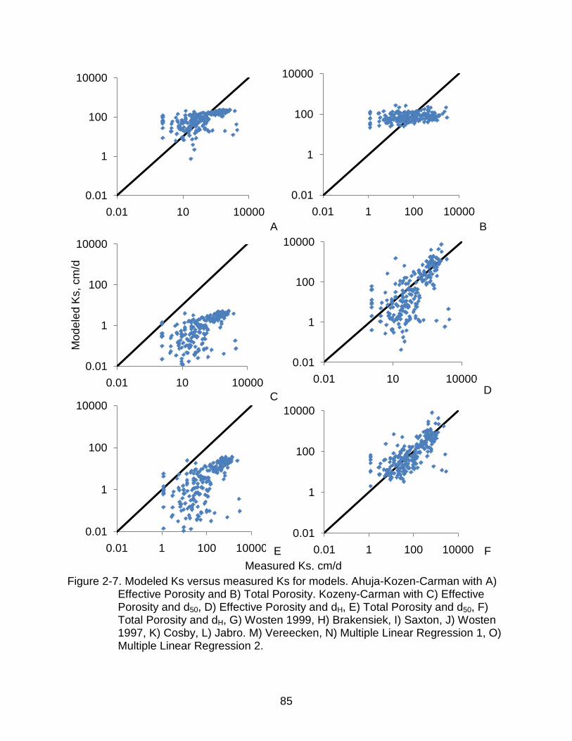
85
Figure 2-7. Modeled Ks versus measured Ks for models. Ahuja-Kozen-Carman with A) Effective Porosity and B) Total Porosity. Kozeny-Carman with C) Effective Porosity and d50, D) Effective Porosity and dH, E) Total Porosity and d50, F) Total Porosity and dH, G) Wosten 1999, H) Brakensiek, I) Saxton, J) Wosten 1997, K) Cosby, L) Jabro. M) Vereecken, N) Multiple Linear Regression 1, O) Multiple Linear Regression 2.
0.01
1
100
10000
0.01 10 100000.01
1
100
10000
0.01 1 100 10000
0.01
1
100
10000
0.01 10 10000
Mod
eled
Ks,
cm
/d
0.01
1
100
10000
0.01 10 10000
0.01
1
100
10000
0.01 1 100 100000.01
1
100
10000
0.01 1 100 10000
A B
C D
Measured Ks, cm/d E F

86
Figure 2-7. Continued
0.01
1
100
10000
0.01 1 100 100000.01
1
100
10000
0.01 1 100 10000
0.01
1
100
10000
0.01 1 100 100000.01
1
100
10000
0.01 1 100 10000
0.01
1
100
10000
0 10 100000.01
1
100
10000
0.01 1 100 10000
Measured Ks, cm/d
Mod
eled
Ks,
cm
/d
G H
I J
K L

87
Figure 2-7. Continued
0.01
1
100
10000
0.01 1 100 100000.01
1
100
10000
0 1 100 10000
0.01
1
100
10000
0 10 10000
Measured Ks, cm/d
Mod
eled
Ks,
cm
/d
M N
O
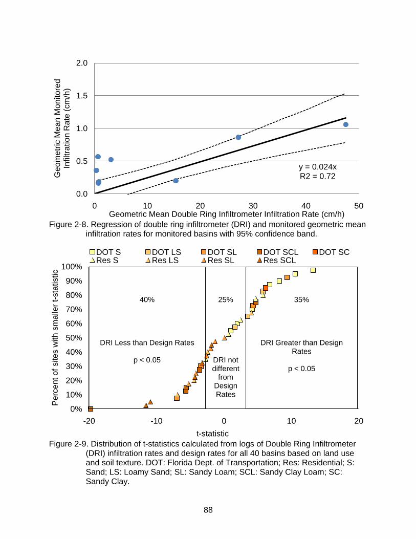
88
Figure 2-8. Regression of double ring infiltrometer (DRI) and monitored geometric mean
infiltration rates for monitored basins with 95% confidence band.
Figure 2-9. Distribution of t-statistics calculated from logs of Double Ring Infiltrometer
(DRI) infiltration rates and design rates for all 40 basins based on land use and soil texture. DOT: Florida Dept. of Transportation; Res: Residential; S: Sand; LS: Loamy Sand; SL: Sandy Loam; SCL: Sandy Clay Loam; SC: Sandy Clay.
y = 0.024xR2 = 0.72
0.0
0.5
1.0
1.5
2.0
0 10 20 30 40 50
Geo
met
ric M
ean
Mon
itore
d In
filtra
tion
Rat
e (c
m/h
)
Geometric Mean Double Ring Infiltrometer Infiltration Rate (cm/h)
0%
10%
20%
30%
40%
50%
60%
70%
80%
90%
100%
-20 -10 0 10 20
Per
cent
of s
ites
with
sm
alle
r t-s
tatis
tic
t-statistic
DOT S DOT LS DOT SL DOT SCL DOT SCRes S Res LS Res SL Res SCL
25%
DRI not different
fromDesign Rates
40%
DRI Less than Design Rates
p < 0.05
35%
DRI Greater than Design Rates
p < 0.05

89
Figure 2-10. Example of size and diversity of vegetation in basin 9. Soil textue: sandy
clay. Land use: Department of Transportation.

90
Figure 2-11. Limited vegetation size and diversity in basin 39. Soil texture: loamy sand.
Land use: Department of Transportation.

91
Figure 2-12. Photo of basin 8 during double ring infiltrometer testing. Soil texture: sandy
loam. Land use: residential.

92
CHAPTER 3 SOIL AMEMDMENTS FOR COMPACTED SOIL MITIGATION I: HYDROLOGY
Introduction
Gregory et al. (2006) showed that soil compaction coinciding with typical
development activities and vehicle traffic reduced infiltration rates from between 23 and
65 cm/h to between 1 and 19 cm/h and increased bulk densities from between 1.20 and
1.42 g/cm3 to between 1.48 to 1.52 g/cm3 on fine sand soils in North Central Florida. Pitt
et al. (1999b) reported a similar decrease of infiltration rates from 41.4 cm/h to 6.4 cm/h
on sandy soils in Alabama.
Current development practices leave soils compacted from heavy equipment
traffic, with reduced porosity, infiltration rates, and increased runoff volumes and rates.
Agricultural lands are commonly selected for these new development sites, increasing
the potential for accumulated pollutants, especially nutrients, in the soil to be
transported by runoff into surface waters. Surface water impairment in Florida is largely
a result of excess nutrients, which can lead to low dissolved oxygen. Low dissolved
oxygen has been attributed to hydrologic modifications and pollution discharges. In
addition, fertilizers applied to agriculture and residential lawns are large nitrate
contributors to groundwater. (2006 Florida 305b Report)
Soil amendments have previously been studied to evaluate their potential for
improving soil properties, mostly in agricultural settings. Two soil amendments, compost
and fly ash, have potential to improve soil properties. Both soil amendments have been
found to decrease bulk density and improve soil moisture holding capacity (Pitt et al.
1999b; Cogger 2005; Khandekar et al. 1997; Gangloff et al. 2000; Adriano and Weber
2001). Fly ash, a bi-product of coal burning, is mostly comprised of silt sized particles

93
(Torrey 1978). Bulk densities range from 0.79 to 1.16 g/cm3 and particle densities from
2.14 to 2.48 g/cm3 (Torrey 1978; Pathan et al. 2003). Most research on the effect of fly
ash incorporation on soil infiltration has found that infiltration rates significantly decrease
(Campbell et al. 1983; Gangloff et al. 2000; Kalra et al. 1998; Pathan et al. 2003). This
has been attributed to the cementing properties of fly ash, which have been utilized to
stabilize soils from deformation (Consoli et al. 2001). However, a few studies have
found that fly ash either was no influence (Adriano et al. 2002) or increased infiltration
rates (Chang et al. 1977).
Though compost is produced from a wide range of parent materials, studies have
shown that compost incorporation typically increases infiltration rates, decreases bulk
density, and increases porosity (Pitt et al. 1999b; Cogger 2005). However the potential
exists for compost to become a source for nutrients in runoff or leachate, depending on
the parent material of the compost and potential for plant uptake (Cogger 2005; Jaber et
al. 2005; Gilley and Eghball 2002).
This study sought to evaluate the hydrologic effects of incorporating two soil
amendments into compacted soils by measuring differences in runoff volumes,
infiltration rates, and soil structure.
Materials and Methods
The study site was located on the University of Florida campus in Gainesville, FL.
Forty two fiberglass lysimeters, measuring 0.76 m x 0.76 m x 0.76 m, were
manufactured for this study. Lysimeters had two 2.5 cm diameter horizontal outlets
installed; one each for runoff and leachate collection (Figure 3-1). The outlets were
centered on the same side and the leachate outlets were typically within 3.8 cm of the
lysimeter bottom, while the runoff outlets were typically 5.0 cm below the top lip. Well

94
screen (1.3 cm diameter, 0.025 cm slot) was installed from the inside of the bottom
outlet and spanned slightly less than the depth of the tank (Figure 3-2). The exterior of
the leachate outlet was fitted with a 2 cm diameter ball-valve. A wooden footer spanning
the width of the lysimeter was attached to bottom of the lysimeter at both the front and
rear. These footers raised the lysimeters above the ground which allowed a forklift to
transport the lysimeters into their final positions, after being filled.
The soils used in this study were Arredondo fine sand (A) and Orangeburg loamy
fine sand (O). The Arredondo soil was collected from a site on the University of Florida
campus while the Orangeburg soil was collected from a stockpile at the North Florida
Research and Education Center near Quincy, FL. The Orangeburg soil was screened to
remove aggregates prior to filling lysimeters.
Two soil amendments used in this study were Black Kow® composted dairy cow
manure (0.5-0.5-0.5; N-P-K respectively) (C) and Class F fly ash (F) from the
Gainesville Regional Utilities (GRU) Deerhaven power plant. Black Kow® is a
composted cattle manure product produced by the Black Gold Composting Co. from
Oxford, FL, that is commonly available to consumers at home and garden retailers.
Soil and amendment characteristics are summarized in Table 3-1. Both soils and
amendments were analyzed for texture by particle-size analysis (ASTM 2007a).
Standard maximum proctor densities were also determined from samples of each soil
(ASTM 2007b). Particle density was measured for each soil and amendment as well
(Blake and Hartge 1978). In addition, organic matter was quantified for five samples of
each soil and amendment by Loss On Ignition (LOI) (Heiri et al. 2001) (Table 3-1).

95
The study timeline was split into three phases: non-compacted, compacted, and
amended. The non-compacted phase began with construction and lasted until soil
compaction began, the compacted phase ran from compaction through amending, and
the amended phase ran from amending until study completion. The leachate valve
remained open during the first two phases. However, the valve was closed for amended
phase events to allow water quality sample collection.
Non-compacted Phase
This study initiated with filling 42 lysimeters in September 2008. Between 20 and
25 cm of No. 57 (ASTM 2003a) quartz stone was laid in the bottom of each lysimeter.
Quartz was selected due to its relatively inert chemical properties. A layer of geotextile
was installed over the drainage layer to prevent soil from settling into the drainage layer
pore space or moving around the edges of the filter fabric. Approximately 50 to 55 cm of
soil was transferred into each lysimeter. A front end loader was used to transport soils
from stockpiles on site to the lysimeters where they were completely filled with soil
(Figure 3-3). The Orangeburg soil was also screened to remove large stones and
aggregates during lysimeter filling; screen openings measured 7.6 cm by 3.8 cm.
Lysimeters were then moved into place by forklift (Figure 3-4). The locations of the
lysimeters were randomized based on treatments to be applied to the soils.
Soils were allowed to settle for approximately eight months until data was
collected from the non-compacted soil at the end of April and beginning of May 2009.
To control vegetation establishment, lysimeters were sprayed for the first 3 months and
then covered with sunlight blocking fabric for the remaining 5 months. After filling the
lysimeters, soil surfaces were above the runoff outlets, resulting in no runoff collection
during this phase.

96
In February 2009 each lysimeter had one horizontal Acclima Digital TDT soil
moisture sensors installed approximately 15 cm below the soil surface. In addition, one
of the three treatment replicate lysimeters also had a vertical profile of sensors installed.
Profile sensors were installed to monitor different soil layers within the lysimeter. Profile
sensors were installed to maximize the cumulative sensing depth between the three
sensors (Figure 3-5). Data from the 84 sensors was collected hourly by two CS 3500
controllers. However, during May and June 2009 nearly all sensors failed due to a
manufacturing defect. All sensors were replaced in coordination with amendment
incorporation in September 2009. It would have been necessary to remove the sensors
from respective lysimeters prior to incorporation regardless of failures to prevent
damage to sensors and cables. However, control lysimeters would not have needed to
be disturbed. In addition, some profile sensors may not have required removal either.
Disturbed areas within control lysimeters were limited during sensor replacement and
were subsequently re-compacted under the final compaction iteration conditions.
Bulk density, infiltration rate, and cone penetrometer measurements were
collected from each lysimeter the week prior to compaction. Bulk density measurements
were performed using the intact core method (Blake and Hartge 1986). The infiltration
rate measurement procedure was based on ASTM (2003b) D-3385 using a double ring
infiltrometer. To maintain a constant head in the inner ring, a Mariotte siphon was used,
while a manually controlled water supply tank was used to maintain an equivalent head
in the outer ring. As a result, the rate of water replenishment to maintain the constant
head within the inner ring was equivalent to the vertical infiltration rate. Due to the high
infiltration rates of these soils, measurements were continued until either the outer tank

97
or Mariotte siphon water was exhausted. Infiltration equipment was calibrated prior to
testing. Infiltration rates were estimated by regression of the infiltration rates and
cumulative infiltration depth using a simplification of the infiltration Green-Ampt model:
𝑓𝑓 = 𝑆𝑆 𝐹𝐹 + 𝐵𝐵⁄ (3-1)
where f is the infiltration rate (cm/h), F is the cumulative infiltration (cm), A is the product
of multiple soil parameters, and B is the infiltration rate at 1/F = 0 (Green and Ampt
1911).
A Field Scout SC 900 Cone Penetrometer (Spectrum Technologies, Inc.,
Plainfield, Illinois) was used to collect cone index profiles. The cone penetrometer had a
maximum depth of 45 cm and a resolution of 2.5 cm. The penetrometer measured the
force applied to drive the cone tip deeper into the soil profile. Three profiles were
collected from each lysimeter.
A rainfall simulator (RFS) was constructed in the event sufficient natural rainfall did
not occur and to add control over rainfall rates and depth applications. The RFS was
supplied by a groundwater well at 240 kPa located approximately 40 m from the
simulator. From the connection, a 2.5 cm PVC water line split into two 2.5 cm water
lines. Four spray nozzles were each connected to the supply lines through a 138 kPa
pressure regulator, for a total of 8 spray heads. The RFS was divided into two rows of
four bays; each bay with one spray nozzle. Plastic curtains were added to the rainfall
simulator frame to block over spray between bays and reduce wind effects.
The RFS was operated for 32 minutes with curtains on April 16, 2009, and without
curtains on April 18, 2009 to evaluate the application uniformity. After each simulation,

98
catch can volumes were recorded and divided by the opening cross-sections (57.8 cm2)
to determine rainfall depths.
Rainfall depths were analyzed to evaluate the uniformity of the RFS. The low
quarter distribution uniformity, DUlq,was calculated as:
𝐺𝐺𝐿𝐿𝑙𝑙𝑞𝑞 = 𝜑𝜑𝑙𝑙𝑞𝑞 𝜑𝜑⁄ (3-2)
where d is the average depth for all catch cans and dlq is the average depth for the
lowest quarter of observations. The UC was calculated by:
𝐿𝐿𝐶𝐶 = 1 − (𝑦𝑦 𝜑𝜑⁄ ) (3-3)
where y is the average of the absolute values of the deviations in collected depth from
the average depth. Values of one for both measurements result from perfect uniformity.
For comparison, catch cans were also distributed prior to a 1.26 cm rainfall event on
April 19, 2009 to determine DUlq and CU for a natural event. A manual rain gauge was
installed under the simulator to capture natural and simulated total rainfall depths. In
addition a HOBO® (Onset Computing Corporation, Bourne, Massachusetts) data
logging tipping bucket rain gauge with a tip resolution of 0.2 mm (RG3-M) was also
installed to measure rainfall rates. Although natural and simulated rainfall events had
variability, distributions were assumed to be uniform and equal to data collected from
the rain gauges.
Compaction Phase
Soil compaction began at the end of April 2009. Gregory et al. (2006) reported that
compacted soils had bulk densities between 1.47 g/cm3 and 1.52 g/cm3, while
undisturbed, or non-compacted, soils had bulk densities ranging from 1.20 g/cm3 to 1.42
g/cm3. These were collected from fine sand texture soils (Apopka and Bonneau). Based

99
on these findings, the threshold compact bulk density of the Arredondo soil was set at
1.45 g/cm3 midway between the maximum non-compacted density and the minimum
compacted density.
A comparable threshold applicable for Orangeburg soils was not found in
literature. However, the Growth Limiting Bulk Density (GLBD) for Arredondo soil was
estimated to be 1.80 g/cm3, compared to 1.64 g/cm3 for Orangeburg based on soil
texture (Daddow and Warrington 1983). Thus the Arredondo threshold of 1.45 g/cm3
was 81% of the GLBD. Assuming a compaction threshold of an equal percent GLBD for
the Orangeburg produces a threshold of 1.32 g/cm3. Both soils received the same
compaction procedure.
The compaction procedure was iterative; bulk densities were measured from three
of the 21 lysimeters for each soil and used as a representative sample to determine
whether the bulk density compaction criteria had been met and determine the effects of
the previous iteration. Four iterations were required to surpass the threshold bulk
densities. Soils were initially compacted using a 25 cm by 25 cm tamper with a single
5.8 kg sliding weight drop. The sliding weight was raised until flush with the top of the
tamper handle and then released (Figure 3-6). The second iteration was two weight
drops. The third iteration was two weight drops after the surface soil had been wetted.
The fourth iteration was two weight drops on wetted soil, but for this iteration the tamper
dimensions had been modified to 12.7 cm x 12.7 cm to enable exertion of more force on
the tamper (Figure 3-7).
Greater bulk densities may have been achieved by using larger compaction
equipment, such as a plate compactor or a ‘jumping jack’ type compactor. However,

100
such equipment was avoided due to the spatial constraints and effort required to move
this size equipment in and out of the lysimeters. In addition, it was unknown if
equipment operation may have applied forces great enough to compromise the
structural integrity of the lysimeters.
Once soils were compacted, bulk density and infiltration rates were measured
again. Measuring cone penetrometer indices leaves voids extending up to 45 cm into
the soil profile. These voids likely would have created preferential flow and hydrologic
response would have been greatly affected. Therefore, cone penetrometer
measurements were not repeated during the compaction phase.
After compaction, the soil level in most lysimeters was below the outlet invert. For
these lysimeters, new outlets were installed to make the outlet invert even with the soil
surface. Runoff was collected in 38 L cylindrical polyethylene tanks. Runoff data
collection began following soil compaction.
Measurement tapes were attached to the side of runoff collection tanks. The tanks
had previously been calibrated for total volume based on water depth. After each event,
depths were recorded and converted to volumes. Volumes were divided by the soil
surface area to determine runoff depths.
Analysis of compacted runoff volumes indicated more runoff was produced than
rainfall fell on some lysimeters. It was later determined that rainfall hitting the lysimeter
flanges was at least partially flowing or splashing into the lysimeters, contributing an
unaccounted for volume. To account for the additional volume, the flange areas were
measured and rainfall depths were scaled up to account for the additional inflow
contributed by the flange areas. Effective rainfall depths were then calculated by

101
multiplying the rainfall by the respective scaling factor for each lysimeter. Prior to the
amendment phase a berm was formed around the inner edge of the flanges to prevent
sheet flow and screening was attached to the flanges to absorb raindrop energy. These
additions were successful in preventing splash and sheet flow from flanges into the
lysimeters.
Amendment Phase
Compacted soils were amended in September 2009. The lysimeters were evenly
divided between soils; 21 each. There were seven treatments (Figure 3-8) combining
amendments (Null (N), C, and F) and incorporation depths (0 cm, 10 cm, and 20 cm).
The seven treatments included all combinations of amendments and depths except for
C and F at 0 cm. Each treatment was replicated three times (Figure 3-8). Lysimeter bulk
densities were ranked for each soil and treatments were applied to a lysimeter from
each of the highest, middle, and lowest seven bulk densities to minimize the effect
compaction variability on results from the subsequent amendment phase. The three
non-amended lysimeters for each soil were controls.
Amendments were applied at 5 cm depth over the area of the lysimeters. A
Craftsman® (Sears Brands, LLC, Hoffman Estates, Illinois) cultivator attached to a
Craftsman® trimmer 4-cycle engine incorporated amendments into the top 10 to 20 cm
of compacted soil. A depth gauge was attached to the cultivator during incorporation to
ensure the accurate depth of incorporation. For 20 cm depths, the incorporation was
done in multiple steps. First, the top 10 cm of compacted soil was removed from the
lysimeter and 2.5 cm of amendment was applied over the exposed soil. The
amendment was then incorporated to down to the 20 cm incorporation depth. The

102
removed soil and remaining amendment were then returned to the lysimeter where they
were incorporated together.
Amending soils raised the soil surface above the outlet inverts. Pipes were cut
through their cross section to form semi-cylinder risers. These risers were installed flush
with the soil surface along the lysimeter side around the runoff outlet. This allowed
runoff to flow from the surface directly into the runoff outlet, which prevented surface
ponding.
After each event, the rainfall depth and runoff volumes were recorded. In addition,
outlets were checked for sediment and cleared if necessary. Soil surfaces were leveled
if necessary following events to limit channeling or depressional storage. The depth
between the top of each lysimeter and the soil surface was measured after most events
to monitor subsidence. As amended soils settled and subsided, risers were adjusted to
remain flush with the soil surface. Bulk densities, infiltration rates, and cone
penetrometer profiles were repeated to complete the amended phase.
Runoff volumes were then used to calculate runoff depths from each lysimeter.
Rainfall and runoff depths were used to calculate runoff coefficients C = Q/P, where C is
the runoff coefficient (unitless), Q is the runoff depth (cm), and P is the rainfall depth
(cm). Runoff depths were calculated by dividing the runoff volume by the respective
lysimeter area. Effective curve numbers (CN) were also calculated using rainfall and
runoff depths, by:
CN = 25400/(254+S) (3-4)
where S is effective maximum storage depth (cm) (NRCS 1986). Rearranging the
NRCS curve number equation,

103
𝑄𝑄 = (𝑃𝑃 − 0.2𝑆𝑆)2 (𝑃𝑃 + 0.8𝑆𝑆)⁄ (3-5)
to solve for S gives:
𝑆𝑆 = 5[𝑃𝑃 + 2𝑄𝑄 − √(4𝑄𝑄2 + 5𝑃𝑃𝑄𝑄)] (Hawkins 1993). (3-6)
Curve numbers were also estimated for each lysimeter during the compacted and
amended phases following the method described by Hawkins (1993). Rainfall and runoff
depth pairs were independently ranked and paired. Storage depths and curve numbers
were then calculated for each pair. Since the Curve Number method assumes a
maximum storage depth, as rainfall depths approach infinity so S and CNs should
approach a constant. This relationship resembles the decaying infiltration rate as it
approaches the saturated hydraulic conductivity. To determine the effective curve
number, the calculated curve numbers are plotted against the inverse of rainfall depths.
The effective curve numbers is assumed to be the intercept or value at 1/P = 0 for the
linear regression of this relationship (Hawkins 1993). Rainfall events which produced no
runoff from a lysimeter were excluded in this analysis.
Infiltration rate distributions were evaluated by Shapiro-Wilk test for normality.
While a few populations passed the test without transformation, after log-transforming
the data virtually all populations were normally distributed. The outstanding populations
were from amended treatments where the sample size was only three, which is difficult
to definitively evaluate the distribution. In addition, infiltration rates have commonly been
found to be log-normally distributed (Logsdon and Jaynes 1996; Haws et al. 2004;
Kosugi 1996), even within relatively close proximity (Sisson and Wierenga 1981).
Therefore, all infiltration rate analyses were performed on log-transformed data.
As a result, the expected value is the Geometric Mean (GM):

104
𝑓𝑓̅ = 10^(∑ log(𝑓𝑓𝑖𝑖)𝑛𝑛𝑖𝑖 /𝑛𝑛), (3-7)
where n is the number of measurements. In addition the geometric standard deviation is
𝐺𝐺𝑆𝑆𝐺𝐺 = 10^��∑ �log(𝑓𝑓𝑖𝑖) − log(𝑓𝑓)����2𝑖𝑖
𝑛𝑛 � /𝑛𝑛 − 1. (3-8)
To determine the range of one GSD, the GM is multiplied and divided by the GSD.
Runoff coefficients were analyzed for significant differences by Wilcoxon Sign Rank
Test for non-parametric comparisons. Curve numbers were analyzed using Tukey’s
multiple pairwise comparison.
Results and Discussion
Based on the LOI testing, the Arredondo soil had a sand texture with 1% OM while
the Orangeburg had a sandy clay loam texture with 5% OM (Table 3-1). Higher organic
matter contents are commonly associated with higher clay content due to reduced
microbial turnover rates (Parton et al. 1987). Orangeburg texture had been listed as
sandy loam in NRCS soil surveys (1993). The maximum proctor density values were
found to be 1.77 g/cm3 for both soils (Table 3-1).
The DUlq and UC were calculated for the rain simulator on various scales: from the
entire simulator down to individual lysimeters (Appendix D). The DUlq and UC for this
event were 0.93 and 0.95, respectively, over the entire RFS area. With curtains, the rain
simulator had an overall DUlq of 0.88 and a UC of 0.92; without curtains only 0.71 and
0.80, respectively. Smaller scale values had higher uniformity for DUlq and UC. In
addition, there was a substantial drop in the uniformity values when the scale increased
from individual lysimeters to bays. However, there was much less decrease for larger
scales. The average rainfall rate was 10.3 cm/h for the two tests. By comparison the

105
half hour intensity for a 10-year return period event for Alachua County, FL is 10.4 cm/h
(Eaglin et al. 2009).
Non-compacted Phase
Non-compacted bulk density ranges from Arredondo and Orangeburg lysimeters
only slightly overlapped (Figure 3-9). Arredondo bulk densities were significantly (p <
0.05) greater than Orangeburg soils. The Arredondo mean bulk density was 14%
greater than the Orangeburg mean; 1.24 g/cm3 compared to 1.07 g/cm3 (Table 3-2).
Variability was essentially equal for the two soils.
Non-compacted Arredondo rates ranged from 111.4 to 196.8 cm/h while
Orangeburg rates ranged from 109.8 to 318.1 cm/h (Figure 3-10, Table 3-3).
Orangeburg rates were significantly (p < 0.05) greater than Arredondo rates, although
only seven Orangeburg rates were greater than the maximum Arredondo infiltration
rate. The Orangeburg GM was 27% greater than Arredondo; 144.5 compared to 178.0
cm/h.
Maximum, minimum, median, and mean cone indices at each depth were
determined for all non-compacted profiles for each soil (Figure 3-11). Both means and
medians overlapped over most of the profiles and decreased with depth. While the
maximum Arredondo profile also decreased with depth, the maximum Orangeburg
profile diverged from this pattern below 25 cm where indices changed erratically with
greater depths. However, this resulted from maximum values coming from only four
profiles within two lysimeters for depths greater than 25 cm. The maximums of the
mean cone indices profiles were 239 and 235 kPa for Arredondo and Orangeburg soils,
respectively. Maximum cone indices were at the surface and generally decreased as

106
depth increased. Orangeburg cone indices were significantly (p < 0.05) greater than
Arredondo at depths between 22.5 cm and 30 cm and at 42.5 cm (Appendix D).
By comparison, the native profiles reported by Gregory et al. (2006) for non-
compacted areas had maximum values at depths of 32, 25, and 32 cm, rather than at
the surface. Profiles from Gregory et al. (2006) showed that the near surface values
started at effectively zero and increased with depth to the maximums at the peak in a
parabolic curve, after which they decreased along the parabolic path until the 45 cm
depth limit. While the maximum value of the Arredondo profiles was profiles was 239
kPa and decreased to a minimum value of 86 kPa at the depth limit of 45 cm, maximum
values from Gregory et al. (2006) were approximately 1,000, 2,600, and 1,800 kPa, for
the natural wood lot and the two planted forest lots, respectively. Thus the natural soil
profiles had much greater cone indices, by almost an order of magnitude, than the
Arredondo profiles. This likely due to the lysimeter construction method which did not
compact soil layers. Filling lysimeters in lifts or layers and ensuring these layers were
compacted to representative bulk densities may have resulted in more representative
cone index profiles.
Infiltration rates and bulk densities were not found to be significantly (p < 0.05)
correlated for either soil (Table 3-4). Cone indices and bulk densities were only
significantly (p < 0.05) correlated for Arredondo soils at 42.5 cm (Table 3-5). The lack of
evidence for a relation between bulk density and infiltration rate was unexpected since
the two parameters are typically linked through porosity and pore size distribution.
However, the low correlation may have resulted from the unconsolidated state of the
soils due to reconstruction.

107
Compacted Phase
Bulk densities
The compaction procedure increased the bulk densities with each iteration (Figure
3-12). Soil samples were collected from three random lysimeters for each soil following
each compaction iteration. However, the initial and final data points in Figure 3-12 show
the minimums, medians, and maximums for all 21 lysimeters for each soil. Therefore,
the bulk density ranges for the first and last iterations were greater than the three
iterations in between, when only three samples were taken. Bulk densities taken after
compaction iterations are listed in Table 3-6 for Arredondo lysimeters and in Table 3-7
for Orangeburg lysimeters. The first iteration, single drop, increased bulk densities the
most of any iteration on both soils. The second iteration, double drop had the least
increase for both soils (Arredondo: 0.03 g/cm3 and Orangeburg: 0.04 g/cm3). The bulk
density increase by the third and forth iterations were approximately opposite for the two
soils. Arredondo bulk densities increased 0.06 g/cm3 on the third iteration and 0.11
g/cm3 on the fourth iteration, while the Orangeburg increased 0.10 g/cm3 on the third
iteration compared to 0.05 g/cm3 on the final iteration.
All Arredondo and Orangeburg lysimeter bulk densities were greater than the
respective thresholds. Compacted bulk densities for Arredondo lysimeters ranged from
1.50 to 1.59 g/cm3 and from 1.36 to 1.55 g/cm3 for Orangeburg lysimeters (Table 3-8).
Arredondo compacted bulk densities were significantly greater than Orangeburg (p <
0.05). Compacted bulk densities for both soils were significantly (p < 0.05) greater than
non-compacted. Mean Arredondo bulk densities increased 0.32 g/cm3 (26%) while
Orangeburg bulk densities increased 0.37 g/cm3 (35%). Arredondo mean bulk density
was 88% of proctor density while Orangeburg mean bulk density was 82% of proctor

108
density. Compacted bulk densities were not significantly (p < 0.05) correlated to non-
compacted bulk densities for either soil.
The compacted percentages of GLBD ranged from 83 to 88% for Arredondo and
from 83 to 95% for Orangeburg. By comparison, Bartens et al. (2008) compacted clay
soils which had GLBDs between 1.45 and 1.55 g/cm3 to two bulk densities, 1.31 and
1.59 g/cm3. The lesser of the two compacted soils were between 84% and 90% of the
GLBD. Thus, the Orangeburg lysimeters were compacted to similar percentages of
GLBD as Bartens et al.(2008) and slightly higher percentages than the Arredondo soil.
Therefore, both Arredondo and Orangeburg soils met the compaction criteria.
Infiltration rates
While Arredondo surface soil bulk densities were comparable to those found by
Gregory et al. (2006), infiltration rates were about 25 cm/h greater than those reported
by Gregory et al. (2006) and Pitt et al. (1999) for compacted urban sandy soils.
Compacted Arredondo infiltration rates ranged from 29 cm/h to 44 cm/h while
Orangeburg rates ranged from 0.3 cm/h to 14.9 cm/h (Table 3-9). Arredondo rates were
significantly (p < 0.05) greater than mean infiltration rates reported by Gregory et al.
(2006) which ranged from 6.4 to 9.1 cm/h. A lack of subsoil compaction may indicate
why infiltration rates were greater than those reported by Gregory et al. (2006) and Pitt
et al. (1999), even though surface bulk densities were comparable.
Compacted infiltration rates for both soils were significantly (p < 0.05) less than
non-compacted rates. The Arredondo GM infiltration rate decreased by a factor of four
after compaction, while the Orangeburg GM infiltration rate decreased by a factor of 43.
The compacted Orangeburg infiltration rate GSD (2.9 cm/h) was much greater than both
non-compacted GSD (1.2 cm/h and 1.3 cm/h) and the compacted Arredondo GSDs (1.1

109
cm/h), indicating a greater variability between these measurements. Bulk densities and
infiltration rates were not significantly (p < 0.05) correlated for either soil. Compacted
infiltration rates were not significantly correlated to non-compacted infiltration rates for
either soil, indicating there was no bias of non-compacted infiltration rates on
compacted rates.
Figure 3-13 shows the relationship between bulk densities and infiltration rate with
respect to compaction for each soil. As bulk densities increased, infiltration rates
decreased logarithmically. While infiltration rates decreased much more for Orangeburg
than Arredondo, bulk density increases were comparable.
Infiltration rates on the order of 100 cm/h, which would not be expected below
compacted in situ soil profiles, were attributed to limited subsoil compaction in
lysimeters. Had the subsoils been representative of compacted soil profiles, infiltration
rates of amended soils likely would have been much lower.
Rainfall and runoff data
Scaling factors were calculated as the ratio of the combined flange and soil
surface area to soil surface are alone. Factors ranged from 1.41 to 1.59, with a median
of 1.44 (Table 3-10) and when applied to rainfall depths assumed all flange rainfall
contributed to the soil surface. Since the volume of additional rainfall contributed to the
lysimeters by the flanges was unknown, it was estimated that the entire flange area was
contributing inflow to the lysimeter. However, flange rainfall may have flowed over the
edges as well.
Runoff data were collected from seven natural events and one RFS (simulated)
event run during the compacted phase. Natural event depths ranged from 1.28 cm to
3.70 cm with an average of 2.39 cm. The simulated event depth was 4.43 cm. However,

110
to account for all rainfall contributing to the lysimeters rainfall was multiplied by the
scaling factor to determine the effective rainfall depth. Incorporating scaling factors, the
effective natural depths ranged from 1.84 cm to 5.32 cm, while the effective simulated
depth was 6.37 cm (Table 3-11).
Runoff coefficients and curve numbers
Runoff coefficients and effective CNs were calculated from rainfall and runoff from
each lysimeter for each event (Appendix D). Curve numbers were not calculated for
lysimeters from events which produced no runoff (Hawkins 1993). In general the
Orangeburg lysimeters produced more runoff and thus higher runoff coefficients and
effective curve numbers than the Arredondo soil. While the ranges overlapped for all
events, the maximum Orangeburg CNs were comparable to the median Arredondo CNs
and average CNs from each storm were greater for Orangeburg than for Arredondo. At
least one Arredondo and Orangeburg lysimeter produced no runoff from at least six
events. Event median runoff coefficients ranged from 0.02 to 0.42 for Arredondo
lysimeters and 0.06 to 0.70 for Orangeburg lysimeters (Table 3-12). Event median
effective CNs ranged from 64 to 83 for Arredondo lysimeters and 71 to 92 for the
Orangeburg lysimeters. Event CNs for average rainfall and runoff depths ranged from
60 to 82 for Arredondo and from 68 to 91 for Orangeburg lysimeters. Rainfall and runoff
depths were also used to calculate effective CNs for each lysimeter. Average effective
CNs for soils were 88 and 94 for Arredondo and Orangeburg, respectively (Table 3-13).
By comparison, the CN for commercial land use on A and B soils are 89 and 92,
respectively (NRCS 1986). Event runoff coefficients and effective curve numbers for
each soil were not highly correlated to infiltration rate or bulk density measurements; all
correlation coefficients had absolute values were less than 0.55.

111
Cone index profiles
Cone index profiles were not taken during the compacted phase since
measurements would create voids extending the entire soil profile likely altering
hydrologic response during compacted and amended phases. However, profiles were
collected just before the amendment phase on the control lysimeters which remained
compacted. Median cone index profiles of non-compacted and compacted states are
shown in Figure 3-14 for both soils. These profiles show that the soil surface decreased
by 5 and 10 cm for Arredondo and Orangeburg soils, respectively. In addition, while the
cone index profiles were essentially the same during the non-compacted phase, the
Arredondo had much higher cone indices along the entire profile than the Orangeburg
soils. Both compacted profiles increased from the soil surface until reaching a maximum
where profiles decreased and approached a constant rate of decrease in index with
depth. The maximum cone index for Arredondo soils was 10 cm below the compacted
soil surface and 5 cm below the Orangeburg compacted soil surface. The increase in
cone index indicates the limiting infiltration layer. Compaction effects seemed to be
limited to the top 30 cm of the non-compacted profile, or 20 and 25 cm for compacted
Orangeburg and Arredondo soils. Below 30 cm, the compacted profiles are similar in
changes with depth to the non-compacted profiles, except offset by 200 and 300 kPa for
Orangeburg and Arredondo, respectively. The change in cone indices below 30 cm may
have resulted from reduced soil moisture resulting from decreased infiltration after
compaction.
The maximum cone indices for compacted Arredondo and Orangeburg lysimeters
were 600 and 770 kPa and occurred at depths of 5 cm and 10 cm below the soil
surface, respectively. By comparison, post-development cone index profiles from

112
Gregory et al. (2007) had maximum values between 4000 and 4500 kPa at depths
between 27.5 cm and 37.5 cm below the surface.
Although Arredondo infiltration rates were well above those reported by Gregory et
al. (2006), effective curve numbers and runoff coefficients typically exceeded values
expected from compacted for A and B soils (“Dirt Roads”, NRCS 1986). Compacted
phase runoff coefficients and curve numbers were conservative due to flange rainfall
contributions. Therefore, the compaction procedure produced hydrologic relationships
representative of compacted soils. However, based on infiltration rates, runoff
production should have been much lower. This may indicate that infiltration rates
measured by double-ring infiltrometer did not accurately measure the hydrologic
performance.
Amendment Phase
Bulk densities
Bulk density values were measured from samples collected from each lysimeter
after amendments were incorporated and are summarized in Table 3-14. An analysis of
variance was used to quantify the effects of the amendments and incorporation depths
on bulk densities for both soils (Table 3-15). All coefficient estimates were significant (p
< 0.05), indicating that, at least when combining the soils data, altering incorporation
depth or amendment type for a soil would significantly change the bulk density.
However, increasing incorporation depth from 10 to 20 cm had the smallest and least
significant effect on the bulk density. Multiple linear regression was also performed on
the bulk density data (Table 3-16). The resulting model, using coefficient estimates
resulted in a RMSE of 0.07 g/cm3. Soils had significantly (p < 0.05) different bulk
densities.

113
Significant differences between treatments were determined using Tukey-Kramer
multiple pairwise comparisons (SAS Institute 2001). Bulk densities were significantly
lower than the control for all fly ash and compost amended soils and null incorporation
at 10 cm for Orangeburg soils. Compost decreased bulk densities the most for both
soils, followed by fly ash and then null. Except for the Arredondo null incorporations, the
deeper incorporation had insignificantly higher bulk densities than the shallow
incorporation depths. Incorporating the same amendment volume into a larger volume
of soil reduced the amendment fraction of the amended soil. Therefore, the
amendment’s effect of reducing bulk density was diminished by diluting the amendment.
Cone index profiles
Three cone index profiles were measured on each lysimeter at the end of the
amendment phase to prevent affecting other soils measurements. Median treatment
cone index profiles are shown in Figure 3-15 through Figure 3-20 with respective soil
control profiles. Paired t-test analyses were performed between cone indices at
common soil depths to the respective controls to determine treatment effects on soil
strength (Appendix D). Cone index values were significantly (p < 0.05) less than control
(compacted) values for all treatments to depths of the respective incorporation.
Profiles show that both 10 and 20 cm incorporation depths were below the depth
of maximum cone index for the compacted soils and 20 cm incorporations may have
eliminated compacted soil layers completely for Orangeburg soils. Thus the limiting
layer, or layer of maximum compaction, was eliminated allowing for increased
infiltration. For Arredondo soils, the 20 cm treatment cone index values approached the
same values for 10 cm treatment and control profiles below 20 cm depth. This indicates
the bottom of the compacted Arredondo soil layer may not have been affected by the 20
114
cm incorporation depth. Gregory et al. (2006) showed that the limiting layer within
compacted cone index profiles was approximately 25 cm below the surface, and
Randrup and Lichter (2001) reported that compaction effects can exceed 40 cm below
the soil surface. Thus, while incorporation depths may have partially or completely
eliminated the limiting soil layer in this study, the same treatments would not be
expected to exceed the compacted soil layer depth on compacted in situ soil profiles.
Significant differences were also found to extend below incorporation depths for multiple
treatment profiles. These phenomena may have occurred due to increased soil moisture
at these depths which may have resulted from increased infiltration for null and compost
amended treatments and increased soil moisture holding capacity from fly ash amended
treatments. Fly ash tends to have a texture dominated by silt sized particles, shifting the
particle size distribution for respective treatments to smaller sizes. As a result, the pore
size distribution may have shifted to increase the water content at field capacity. Soil
moisture variability can change soil strength and change the soil response to applied
forces. In addition, more Orangeburg profiles had significant differences below the
designated incorporation depth than Arredondo (Table 3-21). The Orangeburg likely had
higher soil moisture content at field capacity, based on texture and resultant pore size
distribution.
Compost incorporated to a depth of 20 cm produced significantly lower cone index
profiles below the incorporation depth. This may have also been due to increased
infiltration and soil moisture which can affect soil strength and cone index readings.
Infiltration rates
An analysis of variance was used to quantify the effects of the amendments and
incorporation depths on infiltration rates for both soils (Table 3-17). All coefficient

115
estimates were significant (p < 0.05). Therefore, all depths and amendments had
significant effects. Comparing geometric means of all treatments found that each was
significantly different when compared to the control and each amendment and depth
was significant (Table 3-18). Multiple linear regression was also performed on the log-
transformed infiltration data (Table 3-19). The resulting model, using coefficient
estimates resulted in a RMSE of 0.327. Converting from log-transformed data, this is a
multiplying factor of 2.12.
Geometric mean and standard deviations of infiltration rates from amended
Arredondo and Orangeburg lysimeters are summarized in Table 3-20. The mean control
infiltration rates were 24.7 cm/h and 1.6 cm/h for Arredondo and Orangeburg lysimeters,
respectively. For Arredondo soils, the fly ash incorporation significantly decreased the
infiltration rates (10 cm: 4.4 cm/h; 20 cm: 12.7 cm/h) compared to 24.7 cm/h for the
control; the difference was significant at 10 cm incorporation. Null incorporation at 20
cm significantly increased the infiltration rates to 84 cm/h, and while rates increased at
10 cm to 39.6 cm/h, the difference was not significant. Null and compost incorporations
to 10 cm (39.6 cm/h and 75.7 cm/h, respectively) and 20 cm (84 cm/h and 92.7 cm/h,
respectively) on Arredondo soils were not significantly different.
For Orangeburg soils, the minimum infiltration rate, 1.6 cm/h, was the control. Both
fly ash amended treatments, 5.0 cm/h at 10 cm and 6.5 cm/h at 20 cm/h, were not
significantly (p < 0.05) different from the control or between the two incorporation
depths. Tillage (null incorporation) significantly (p < 0.05) increased infiltration rates with
deeper incorporation depths, from 1.6 cm/h to 9.3 cm/h to 94 cm/h for 0, 10, and 20 cm
incorporation depths. The highest infiltration rates were from compost treatments at 10

116
cm (105.7 cm/h) and 20 cm/h (112.1 cm/h). Infiltration rates for tillage at 20 cm and 10
and 20 cm compost incorporations were not significantly different.
Infiltration rates for 10 cm tillage were significantly greater on Arredondo than
Orangeburg soil. However, Orangeburg infiltration rates were greater than Arredondo
(not significantly) for three other treatments: null incorporation at 20 cm and both
compost depths. The limiting layer was only 5 cm below the compacted soil surface for
the Orangeburg soil but was 10 cm below Arredondo compacted surface based on
control treatment cone index profiles. Comparing 20 cm compost incorporation and
tillage only cone penetrometer profiles, residual effects of compaction remained below
the incorporated depth on the Arredondo soil while the Orangeburg profiles have no
remaining compaction. As previously noted the non-compacted infiltration rates for
Orangeburg soils were greater than the Arredondo soils. Thus the combination of
insufficient subsoil compaction and a shallower compaction layer which was more fully
eliminated produced greater infiltration rates for Orangeburg treatments and would not
be expected on real world soil profiles.
Runoff coefficients
During the amendment phase 9 natural and 10 simulated events fell on the
lysimeters (Table 3-22) with depths ranging from 0.4 to 11.4 cm. Runoff coefficients
were calculated as the ratio of rainfall depth to runoff depth. Values for amended
Arredondo and Orangeburg treatments are listed in Appendix D with means in Table 3-
23 and Table 3-24, respectively. Significant differences were determined by analyzing
values with Wilcoxon sign rank test due to the non-parametric distribution of values. The
control treatments (Null, 0 cm) had mean runoff coefficients for the amended phase of
0.21 and 0.41 for the Arredondo and Orangeburg soils. By comparison, runoff

117
coefficients for ¼ acre residential areas, assuming 38% impervious, on A and B soils
are 0.22 and 0.50, respectively (NRCS 1986).
The treatment with the largest runoff production for both soils was fly ash
incorporated at 10 cm. Fly ash amendments incorporated at both depths significantly
increased runoff production from both compacted soils. The treatments with the least
runoff production were from compost treatments; 20 cm incorporation for Arredondo and
10 cm for Orangeburg. Treatments of null or compost incorporated to 10 or 20 cm
significantly decreased runoff coefficients compared to the compacted control. All
Orangeburg treatments were significantly (p < 0.05) different from each other. Three
Arredondo treatments were not significantly different from each other: Null at 10 and 20
cm incorporation and Compost at 10 cm.
Curve numbers
Curve numbers were calculated for runoff producing events from each lysimeter
(Appendix D). These curve numbers were then regressed against the inverse rainfall
depths for each lysimeter. Summarized linear regressions are listed in Table 3-25 and
Table 3-26 for Arredondo and Orangeburg lysimeters, respectively. Mean effective
curve numbers for each treatment are listed in Table 3-27 and Table 3-28 for Arredondo
and Orangeburg soils, respectively.
Fly ash incorporated at 10 cm produced the greatest mean curve number of all
treatments for both soils, followed closely by the 20 cm fly ash incorporations, which
were not significantly different. The mean control curve number for both soils was lower
than both fly ash treatments, although not significantly.
Tillage alone significantly decreased runoff production compared to the control for
both 10 and 20 cm depths. While mean curve numbers were lower on both soils for 20

118
cm tillage compared to 10 cm, the differences were not significant. Compost
incorporations at both depths also significantly decreased mean curve numbers
compared to the controls. However, curve numbers were not significantly different
between compost treatment depths. The lowest mean curve numbers were from tillage
with compost at 10 cm.
Incorporating compost with tillage did not significantly decrease effective curve
numbers compared to tillage alone. Although, mean curve numbers for curve numbers
were lower for 10 cm incorporations. Including an organic amendment would also likely
add horticultural benefits over the absence of amendments, especially in situations
where topsoil has been removed. The increased available organic matter may increase
soil fertility and provide habitat for soil organisms more rapidly than natural
accumulation of organic matter.
The minimum treatment of compacted soils, null amendment at 10 cm for both
soils significantly reduced runoff production compared to the compacted soil and was
not significantly different from deeper tillage. Significant reductions in runoff volumes
can be achieved for small rainfall events with minimal tillage and without including
amendments for these two soil types. This seems to be true especially if the limiting
layer to infiltration is near the surface.
To quantify the potential runoff reduction of 10 cm tillage without amendments
runoff depths were calculated for a hypothetical residential watershed where 0, 50, or
100% of the open area had been treated receiving a 2-yr 24-hour rainfall event for
Gainesville, FL (9.2 cm; Eaglin 1996). All open space was assumed to be compacted
and have curve numbers equal to those found in this study. The watershed assumed an
119
imperviousness of 25%. These values were compared to undisturbed pasture and
wooded areas in fair condition. Results are shown in Table 3-29. Assuming Arredondo
as an A soil and Orangeburg as a B soil, runoff depths were approximately 3/4 and 2/3
of the runoff depth of the non-treated watershed.
Stormwater regulations frequently require mitigating the increased runoff after
development. Since the Arredondo soils had much lower runoff depths under pre-
developed conditions, tillage was not as effective at reducing the additional runoff as on
Orangeburg soils. Thus, the runoff depth differences between pre- and post-
development with tillage were less on Orangeburg soils than on Arredondo soils. As a
result, soil amending may prove to be more effective at mitigating compaction on pre-
developed soils with lower infiltration rates, with respect to runoff generation.
Furthermore, soil amending could offset the costs of conventional stormwater
structures by reducing their size. Without considering land purchase, the costs of
traditional retention basins are a power function of the basin volume (SEWRPC 1991).
Exponents range from 0.51 to 0.75. Thus reducing the runoff volume by half would
reduce costs between 30 and 40%. In addition, the reduced size of a retention basin
would increase the available are for land development, which could be the more
valuable benefit.
Conclusions
Although the compaction procedure produced surface soil bulk densities
comparable, infiltration rates were greater and cone indices were lower than those
reported by Gregory et al. (2006). Thus, insufficient subsoil compaction did not replicate
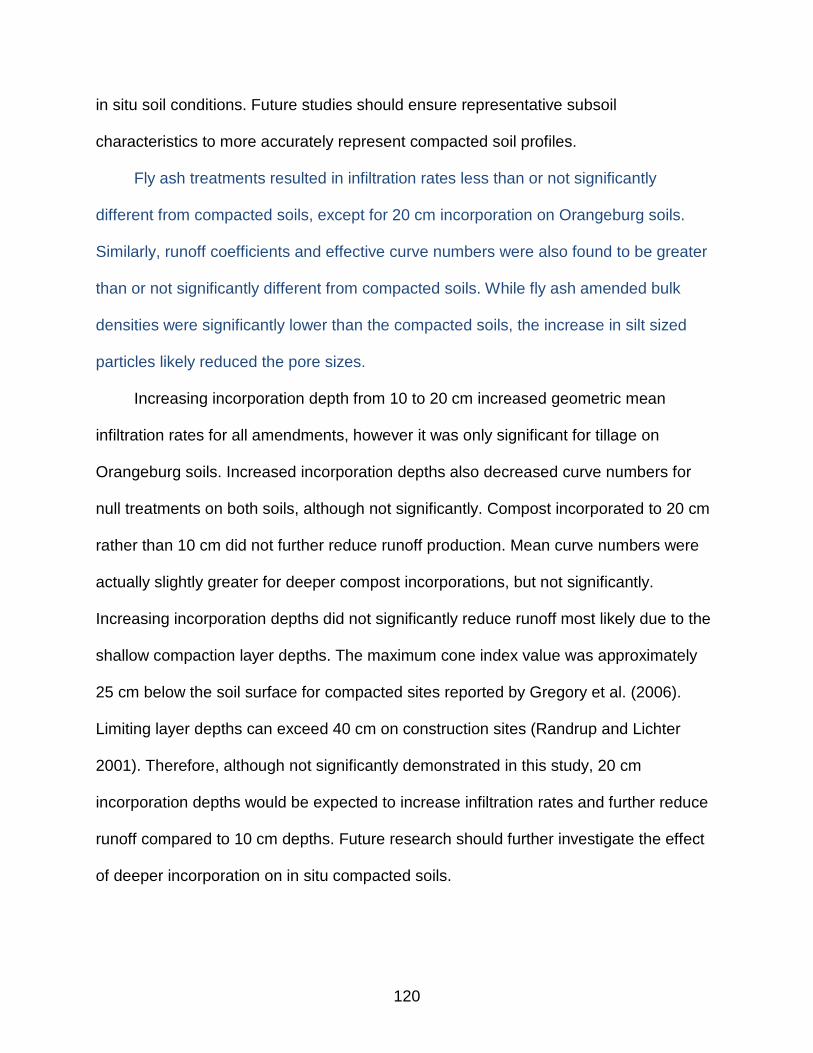
120
in situ soil conditions. Future studies should ensure representative subsoil
characteristics to more accurately represent compacted soil profiles.
Fly ash treatments resulted in infiltration rates less than or not significantly
different from compacted soils, except for 20 cm incorporation on Orangeburg soils.
Similarly, runoff coefficients and effective curve numbers were also found to be greater
than or not significantly different from compacted soils. While fly ash amended bulk
densities were significantly lower than the compacted soils, the increase in silt sized
particles likely reduced the pore sizes.
Increasing incorporation depth from 10 to 20 cm increased geometric mean
infiltration rates for all amendments, however it was only significant for tillage on
Orangeburg soils. Increased incorporation depths also decreased curve numbers for
null treatments on both soils, although not significantly. Compost incorporated to 20 cm
rather than 10 cm did not further reduce runoff production. Mean curve numbers were
actually slightly greater for deeper compost incorporations, but not significantly.
Increasing incorporation depths did not significantly reduce runoff most likely due to the
shallow compaction layer depths. The maximum cone index value was approximately
25 cm below the soil surface for compacted sites reported by Gregory et al. (2006).
Limiting layer depths can exceed 40 cm on construction sites (Randrup and Lichter
2001). Therefore, although not significantly demonstrated in this study, 20 cm
incorporation depths would be expected to increase infiltration rates and further reduce
runoff compared to 10 cm depths. Future research should further investigate the effect
of deeper incorporation on in situ compacted soils.

121
Additional research should also investigate whether the benefits of treatments
extend to a larger scale at either the watershed or plot level. Findings from such study
would hopefully quantify the effects of treatments more accurately, especially with
native soils below the amendment profile. Results presented here have shown there is a
potential to reduce runoff by tilling soil, with or without compost, to depths as shallow as
10 cm. For compacted profiles with limiting layers below the incorporation depth, deeper
incorporations would be expected to improve hydrologic response, especially for larger
rainfall events.
Cost and energy increase as mitigation increases in depth. As depth increases,
the benefits become negligible, no matter the infiltration rate due to the increased
storage capacity of the soil. Even if incorporated depths do not exceed the most limiting
depth of compaction, the available water storage above that layer is increased. In this
way, the amended soil functions similarly to permeable pavement systems, where the
surface layers are not limiting to infiltration, rainfall and runoff are captured and stored
and then infiltrated at a slower rate. Thus, runoff may be significantly reduced,
especially from smaller rainfall events. As a result, soil amending could be incorporated
into low-impact development, which seeks to mimic pre-development hydrology.

122
Table 3-1. Summary of properties for soils and amendments included in this study.
Arredondo Orangeburg Compost Fly Ash
Sand 94 61 81 23 Silt 3 13 11 71 Clay 3 26 8 6
Texture Sand Sandy Clay Loam
Loamy Sand
Silty Loam
Particle Density (g/cm3) 2.41 2.56 2.26 2.10 Organic Matter by LOI% 1 5 79 51 Maximum Proctor Density (g/cm3) 1.77 1.77
Table 3-2. Non-compacted bulk densities. Arredondo Orangeburg
ρb (g/cm3) ρb (g/cm3) Maximum 1.38 1.17
Median 1.23 1.08 Minimum 1.16 0.95 Mean 1.24* 1.07* St. Dev. 0.05 0.05
*Student t-test used to determine that values were significantly (p < 0.05) different. Table 3-3. Non-compacted infiltration rates Arredondo Orangeburg
(cm/h) (cm/h) Maximum 196.8 318.1
Median 140.6 163.4 Minimum 111.4 109.8 Geometric Mean 144.5 178.0 Geometric Standard Deviation 1.2 1.3 *Student t-test used to determine that values were significantly (p < 0.05) different Table 3-4. Pearson correlation coefficients and p-values for non-compacted bulk density
and infiltration rate. Soil r p-value Arredondo 0.23 0.32 Orangeburg 0.07 0.76

123
Table 3-5. Pearson correlation coefficients and p-values for cone indices with bulk densities and infiltration rates.
Cone Indices vs. Bulk Densities Cone Indices vs. Infiltration Rates Soil Depth Arredondo Orangeburg Arredondo Orangeburg (cm) r p-value r p-value r p-value r p-value
0.0 0.06 0.78 0.18 0.43 -0.03 0.91 -0.29 0.21 2.5 0.26 0.26 -0.04 0.88 -0.21 0.37 -0.06 0.78 5.0 0.06 0.79 0.03 0.89 -0.53 0.01 -0.23 0.32 7.5 0.01 0.98 0.08 0.73 -0.32 0.16 -0.28 0.22
10.0 0.11 0.65 -0.07 0.76 -0.18 0.42 -0.26 0.26 12.5 0.08 0.72 -0.04 0.85 -0.04 0.87 -0.31 0.17 15.0 0.05 0.83 -0.08 0.74 0.00 0.98 -0.16 0.50 17.5 0.03 0.91 0.01 0.98 -0.10 0.67 -0.07 0.76 20.0 0.06 0.81 -0.05 0.82 0.03 0.89 -0.05 0.84 22.5 -0.03 0.91 -0.04 0.87 0.03 0.88 -0.10 0.68 25.0 -0.13 0.58 -0.05 0.82 -0.07 0.78 -0.11 0.64 27.5 -0.35 0.12 -0.04 0.88 -0.07 0.77 -0.04 0.87 30.0 -0.22 0.35 0.01 0.98 0.08 0.72 -0.07 0.75 32.5 -0.13 0.56 -0.05 0.84 0.20 0.38 -0.09 0.71 35.0 -0.04 0.85 -0.16 0.49 0.20 0.38 0.08 0.73 37.5 0.10 0.68 0.02 0.92 0.18 0.44 0.19 0.41 40.0 0.31 0.17 0.22 0.34 0.09 0.70 0.25 0.27 42.5 0.45 0.04 -0.24 0.29 0.36 0.11 -0.09 0.69 45.0 0.09 0.70 0.06 0.78 -0.24 0.30 0.20 0.38
Table 3-6. Arredondo bulk densities and mean bulk density increase for each
compaction iteration. Bulk Densities (g/cm3)
Non-compact
Single Drop
Double Drop
Wet Double Drop
Quartered Wet Double Drop
Maximum 1.38 1.39 1.41 1.47 1.59 Median 1.23 1.36 1.40 1.46 1.56 Minimum 1.16 1.33 1.36 1.42 1.50 Mean 1.24 1.36 1.39 1.45 1.56 ρb increase 0.12 0.03 0.06 0.11

124
Table 3-7. Orangeburg bulk densities and mean bulk density increase from each compaction iteration.
Bulk Densities (g/cm3)
Non-compact Single Drop
Double Drop
Wet Double Drop
Quartered Wet Double Drop
Maximum 1.17 1.27 1.26 1.35 1.55 Median 1.08 1.17 1.22 1.31 1.44 Minimum 0.95 1.08 1.15 1.26 1.36 Mean 1.07 1.17 1.21 1.31 1.36 ρb increase 0.10 0.04 0.10 0.05
Table 3-8. Summary of compacted bulk densities and percent of Growth Limiting Bulk
Densities (GLBD). Arredondo Orangeburg g/cm3 %GLBD* g/cm3 %GLBD* Maximum 1.59 88 1.55 95 Median 1.56 87 1.44 88 Minimum 1.50 83 1.36 83 Mean 1.56 87 1.44 88 Standard Deviation 0.02 1 0.05 3
*GLBD for Arredondo: 1.80 g/cm3; Orangeburg: 1.64 g/cm3 (Daddow and Warrington 1983) Table 3-9. Summary of compacted infiltration rates. Arredondo Orangeburg cm/h cm/h Maximum 44.2 14.9 Median 36.4 4.8 Minimum 28.5 0.3 Geometric Mean 36.1 4.1 Geometric Standard Deviation 1.1 2.9

125
Table 3-10. Scaling Factors (SF) calculated for compacted phase as the ratio of soil area and flange area to soil area for each lysimeter. SFs for each lysimeter are applied to the rainfall depth to account for additional rainfall from lysimeter flanges.
Lysimeter SF Lysimeter SF Lysimeter SF 1 1.54 15 1.45 29 1.44
2 1.48 16 1.50 30 1.42 3 1.44 17 1.43 31 1.43 4 1.59 18 1.42 32 1.42 5 1.42 19 1.45 33 1.42 6 1.46 20 1.42 34 1.43 7 1.43 21 1.47 35 1.44 8 1.47 22 1.43 36 1.41 9 1.56 23 1.44 37 1.45
10 1.44 24 1.46 38 1.44 11 1.51 25 1.44 39 1.44 12 1.44 26 1.45 40 1.41 13 1.42 27 1.47 41 1.42 14 1.43 28 1.43 42 1.44
Table 3-11. Rainfall event dates, depth, and effective rainfall depths calculated from the
median scaling factor. Date Type Depth (mm) Effective Depth (mm) 8/4/2009 Natural 31 21 8/6/2009 Natural 43 30 8/7/2009 Simulated 64 44 8/12/2009 Natural 18 13 8/21/2009 Natural 19 13 8/28/2009 Natural 51 36 9/2/2009 Natural 24 17 9/3/2009 Natural 53 37

126
Table 3-12. Summary of compaction phase runoff coefficients for each soil. Rainfall (mm)
44 37 36 30 21 17 13 13
Arredondo Maximum 0.59 0.54 0.15 0.30 0.33 0.07 0.16 0.12 Median 0.42 0.37 0.00 0.09 0.03 0.00 0.00 0.00 Minimum 0.09 0.00 0.00 0.00 0.00 0.00 0.00 0.00 Mean 0.41 0.31 0.04 0.11 0.07 0.01 0.02 0.02 Standard Deviation 0.12 0.17 0.05 0.10 0.08 0.02 0.04 0.03 Orangeburg Maximum 0.91 0.71 0.31 0.64 0.80 0.97 0.37 0.34 Median 0.62 0.53 0.07 0.24 0.46 0.02 0.00 0.00 Minimum 0.38 0.31 0.00 0.00 0.00 0.00 0.00 0.00 Mean 0.65 0.52 0.10 0.27 0.42 0.17 0.09 0.06 Standard Deviation 0.14 0.12 0.11 0.19 0.18 0.29 0.14 0.11
Table 3-13. Summary of compacted regressed curve numbers. Arredondo Orangeburg Maximum 100 100 Median 87 94 Minimum 70 85 Mean 88 94 St. Dev. 9 3
Table 3-14. Mean bulk densities (g/cm3) for each soil for each treatment. Amendment Depth (cm) Arredondo Orangeburg
Mean St. Dev. Mean St. Dev
Null 0 1.51 0.07 a* 1.42 0.07 ab
10 1.35 0.07 abc 1.19 0.03 cdef 20 1.31 0.05 abcd 1.27 0.10 bcde
Fly Ash 10 1.13 0.13 def 1.07 0.05 efg 20 1.23 0.02 bcde 1.18 0.01 cdef
Compost 10 1.01 0.05 fg 0.91 0.04 g 20 1.07 0.07 efg 0.99 0.11 fg
*Values with the same letter are not significantly different. (p < 0.05) Means were analyzed using Tukey multiple pairwise comparison.

127
Table 3-15. ANOVA for amended phase bulk density results.
Source Degrees of Freedom
Sum of Squares
Mean Square Error F-ratio p-value
Model 5 1.156 0.231 49.27 < 0.0001 Soil 1 0.071 0.071 15.18 0.0004 Amendment 3 1.045 0.348 74.16 < 0.0001 Depth 1 0.041 0.041 8.66 0.0057 Error 36 0.169
Total 41 1.326
All interactions were not significant (p<0.05). Table 3-16. Multiple linear regression results of amended bulk densities. Parameter Estimate Standard Error F-ratio p-value Intercept 1.43 0.030 47.67 < 0.0001 Soil
Arredondo 0.08 0.021 3.90 0.0004 Orangeburg -- -- -- -- Amendment
Compost -0.44 0.036 -12.20 < 0.0001 Fly Ash -0.28 0.036 -7.82 < 0.0001 Null -0.15 0.036 -4.22 0.0002 Incorporation Depth
10 cm -- -- -- -- 20 cm 0.07 0.023 2.94 0.0057
Model R2 = 0.872; RMSE = 0.068 Table 3-17. ANOVA for amended phase log of infiltration rates results.
Source Degrees of Freedom
Sum of Squares Mean Square F-ratio P-value
Model 5 15.33 1.18 31.41 <.0001 Soil (S) 1 0.67 0.67 17.94 0.0002 Amendment (A) 3 10.85 3.62 96.31 <.0001 Depth (D) 1 1.02 1.02 27.09 <.0001 S*A# 3 1.78 0.59 15.81 <.0001 A*D 2 0.57 0.28 7.57 0.0024 S*D*A 3 0.44 0.15 3.94 0.0183 Error 36 1.05
Total 41 16.39
#S*D was not significant (p < 0.05)
128
Table 3-18. Summary of log of infiltration rate mean. Contrast Sum of Squares F-ratio p-value Control vs. Treatments 2.319 61.75 <.0001
Depth (cm)
0 vs. 10 1.140 30.37 <.0001 0 vs. 20 3.172 84.47 <.0001 10 vs. 20 1.017 27.09 <.0001 Amendment
Null vs. Compost 0.796 21.18 <.0001 Null vs. Fly Ash 3.853 102.59 <.0001 Compost vs. Fly Ash 8.150 217.01 <.0001
Table 3-19. Multiple linear regression results of log-transformed amended infiltration
rates. Parameter Estimate Standard Error F-ratio p-value Intercept 0.67 0.140 4.71 <.0001 Soil
Arredondo 0.25 0.101 2.51 0.0167 Orangeburg -- -- -- -- Amendment
Compost 1.35 0.172 7.83 <.0001 Fly Ash 0.18 0.172 1.07 0.2925 Null 0.99 0.172 5.72 <.0001 Incorporation Depth 10 cm -- -- -- -- 20 cm 0.34 0.011 3.09 0.0039
Model R2 = 0.765; RMSE = 0.327

129
Table 3-20. Geometric Means (GM) and Standard Deviations (GSD) of amended infiltration rates (cm/h) for both soils.
Treatment
Arredondo Orangeburg Amendment Depth (cm) GM GSD
GM GSD
Null
0 24.7 1.2 bcd* 1.6 2.1 f 10 39.6 1.4 abc 9.3 1.4 de 20 84.0 1.4 ab 94.0 1.3 a
Fly Ash 10 4.4 1.8 ef 5.0 2.7 ef 20 12.7 1.5 cde 6.5 1.7 e
Compost 10 75.7 1.2 ab 105.7 1.0 a 20 92.7 1.1 ab 112.1 1.1 a
*Values with the same letter are not significantly (p < 0.05) different. Geometric means were analyzed using Tukey comparison of means. Table 3-21. Summary of depths from the surface of significant (p < 0.01) difference in
cone index between treatments and controls. Treatment
Arredondo Orangeburg
Amendment Depth (cm) Depth (cm)* Depth (cm)* Null 10 15.0a 20.0 Null 20 27.5 12.5c Fly Ash 10 15.0b 12.5 Fly Ash 20 25.0 22.5a Compost 10 15.0 25.0 Compost 20 15.0 37.5
*Depths are from the surface. Differences were significant (p > 0.05) between surface and 5 cm(a), 10 cm (b), or 15 cm (c).

130
Table 3-22. Amended phase rainfall events and depths which runoff was measured. Date Type Depth (mm) 09/23/09 Simulated 114.4 09/30/09 Simulated 77.2 10/07/09 Simulated 61.6 10/14/09 Simulated 67.3 10/21/09 Simulated 54.7 10/28/09 Natural 4.4 11/04/09 Simulated 75.4 11/10/09 Natural 12.3 11/12/09 Simulated 50.4 11/18/09 Simulated 71.6 11/23/09 Simulated 69.8 11/25/09 Natural 58.8 12/02/09 Natural 14.5 12/05/09 Natural 34.8 12/18/09 Natural 5.4 12/25/09* Natural 6.9
01/01/10 Natural 18.5 (25.4)
01/13/10 Simulated 71.6 01/17/10 Natural 29.5 01/22/10 Natural 19.2
*Event depths from 12/25/09 and 01/01/10 were combined together since collection tanks were not emptied between events. Table 3-23. Summary of amendment phase Arredondo runoff coefficients. Amendment Depth (cm) Mean Coefficient
Fly Ash 10 0.49 a* 20 0.36 b
Null 0 0.21 c
10 0.01 d 20 0.01 d
Compost 10 0.01 d 20 <0.005 e
*Runoff Coefficients with the same letter are not significantly (p < 0.05) different via Wilcoxon paired tests.

131
Table 3-24. Summary of amendment phase Orangeburg treatment runoff coefficients. Amendment Depth (cm) Mean Coefficient
Fly Ash 10 0.45 a* 20 0.45 b
Null 0 0.41 c
10 0.17 d 20 0.11 e
Compost 10 0.08 f 20 0.12 g
*Runoff Coefficients with the same letter are not significantly (p < 0.05) different via Wilcoxon paired tests. Table 3-25. Median slope, intercept, and r2 values for Arredondo curve number
regression against inverse of rainfall depth. Amendment Incorporation Depth (cm) Slope Intercept r2 Null 0 4.4 72 0.66 Null 10 10.4 54 0.71 Null 20 22.8 44 0.92 Fly Ash 10 1.4 90 0.50 Fly Ash 20 1.1 86 0.27 Compost 10 27.1 40 0.95 Compost 20 20.1 48 0.99
Table 3-26. Median slope, intercept, and r2 values for Orangeburg curve number
regression against inverse of rainfall depth. Amendment Incorporation Depth (cm) Slope Intercept r2 Null 0 1.7 86 0.35 Null 10 5.5 71 0.56 Null 20 9.2 62 0.60 Fly Ash 10 1.2 89 0.34 Fly Ash 20 1.9 87 0.52 Compost 10 6.7 61 0.73 Compost 20 11.4 64 0.62

132
Table 3-27. Summarized mean curve numbers for amended Arredondo treatments. Amendment Depth (cm) Mean Curve Number
St. Dev.
Fly Ash 10 91 a* 3 Fly Ash 20 86 ab 4 Null 0 75 b 6 Null 10 49 c 8 Compost 20 44 c 9 Null 20 44 c 1 Compost 10 40 c 2
*Curve numbers with the same letter are not significantly (p < 0.05) different via Tukey-Kramer multiple pairwise comparison. Table 3-28. Summarized mean curve numbers for amended Orangeburg treatments. Amendment Depth (cm) Mean Curve Number
St. Dev.
Fly Ash 10 89 a* 1 Fly Ash 20 88 a 3 Null 0 87 a 2 Null 10 71 b 3 Null 20 64 b 5 Compost 20 62 b 3 Compost 10 62 b 5
*Curve numbers with the same letter are not significantly (p < 0.05) different via Tukey-Kramer multiple pairwise comparison. Table 3-29. Hypothetical runoff depths from a 2-yr 24-hr rainfall event for Gainesville, FL
(9.2 cm) for various percentages of open area treated with tillage at 10 cm compared with undisturbed conditions.
Percent of Open Area Treated*
Runoff Depths (cm)
Arredondo Orangeburg
0% 4.32 6.35 50% 3.28 4.80 100% 2.21 3.25
Undisturbed
Pasture (Fair) 0.50 2.61 Woods (Fair) 0.00 1.48
*Assumed from 25% impervious area with all open area compacted.

133
Figure 3-1. Centerline, cross-sectional diagram of a lysimeter from the left side.
A B Figure 3-2. A) Well screen installed in the bottom of a lysimeter prior to filling. B)
Measurement of drainage layer depth after filling.
A B Figure 3-3. A) Filter fabric installed over drainage layer. B) Screening of Orangeburg soil
during lysimeter filling.

134
A B Figure 3-4. A) Moving filled lysimeter via forklift. B) Lysimeters placed in their respective
locations.
Figure 3-5. Soil moisture sensor diagram.

135
Figure 3-6. Soil compaction using tamper and slide weight.
Figure 3-7. Compaction during final iteration using modified tamper.

136
Figure 3-8. Schematic of lysimeter layout and rainfall simulator. Soil types are identified
for each lysimeter as A (Arredondo) or O (Orangeburg).
Figure 3-9. Non-compacted bulk density values.
0.9
1
1.1
1.2
1.3
1.4
Bul
k D
ensi
ty (g
/cm
3 )
Arredondo Orangeburg

137
Figure 3-10. Non-compacted infiltration rates
Figure 3-11. Maximum, mean, median, and minimum value cone penetrometer profiles
for Arredondo and Orangeburg soils.
100
150
200
250
300
350In
filtra
tion
Rat
e (c
m/h
)
Arredondo Orangeburg
0
5
10
15
20
25
30
35
40
45
0 500
Dep
th (c
m)
Arredondo Cone Index (kPa)
0 500
Orangeburg Cone Index (kPa)
Maximum
Mean
Median
Minimum

138
Figure 3-12. Bulk densities following compaction iterations. Pre = Non-compacted; SD =
Single Drop; DD = Double Drop; WDD = Wetted Double Drop; QWDD = Quartered Wetted Double Drop
0.90
1.00
1.10
1.20
1.30
1.40
1.50
1.60
Pre SD DD WDD QWDD
Bul
k D
ensi
ty (g
/cm
3)
Compaction Iteration
Orangeburg Max. Arredondo Max.
Orangeburg Med. Arredondo Med.
Orangeburg Min. Arredondo Min.
1.45 g/cm3
1.32 g/cm3

139
Figure 3-13. Infiltration rates versus bulk densities for non-compacted and compacted
lysimeters for both soil types.
0.1
1
10
100
1000
0.90 1.00 1.10 1.20 1.30 1.40 1.50 1.60
Infil
tratio
n R
ate
(cm
/h)
Bulk Density (g/cm3)
Arredondo UncompactedArredondo CompactedOrangeburg UncompactedOrangeburg Compacted

140
Figure 3-14. Comparison of median non-compacted and control cone index profiles.
0
5
10
15
20
25
30
35
40
45
0 200 400 600 800 1000D
epth
bel
ow o
rigin
al s
oil s
urfa
ce (c
m)
Cone Index (kPa)
Arredondo Non-Compacted
Orangeburg Non-Compacted
Arredondo Compacted
Orangeburg Compacted

141
Figure 3-15. Median Arredondo null amended cone index profiles. Offset depths are
referenced to compacted soil surface.
0
5
10
15
20
25
30
35
40
45
0 200 400 600 800 1000S
oil
Dep
th (c
m)
Arredondo Cone Index (kPa)
Null 0 cm (control)
Null 10 cm
Null 20 cm
10 cm
20 cm
0 cm

142
Figure 3-16. Median Arredondo compost amended cone index profiles. Profiles are
referenced to the top of the drainage layer. Offset depths are referenced to compacted soil surface.
0
5
10
15
20
25
30
35
40
45
0 200 400 600 800 1000S
oil D
epth
(cm
)Arredondo Cone Index (kPa)
Null 0 cm (control)
Compost 10 cm
Compost 20 cm
10 cm
20 cm
0 cm

143
Figure 3-17. Median Arredondo fly ash amended cone index profiles. Profiles are
referenced to the top of the drainage layer. Offset depths are referenced to compacted soil surface.
0
5
10
15
20
25
30
35
40
45
0 200 400 600 800 1000S
oil D
epth
(cm
)Arredondo Cone Index (kPa)
Null 0 cm (control)
Fly ash 10 cm
Fly Ash 20 cm
10 cm
20 cm
0 cm

144
Figure 3-18. Median Orangeburg null amended cone index profiles. Profiles are
referenced to the top of the drainage layer. Offset depths are referenced to compacted soil surface
0
5
10
15
20
25
30
35
40
45
0 200 400 600 800 1000D
epth
(cm
)Orangeburg Cone Index (kPa)
Null 0 cm (control)
Null 10 cm
Null 20 cm
10 cm
20 cm
0 cm

145
Figure 3-19. Median Orangeburg compost amended cone index profiles. Profiles are
referenced to the top of the drainage layer. Offset depths are referenced to compacted soil surface.
0
5
10
15
20
25
30
35
40
45
0 200 400 600 800 1000D
epth
(cm
)Orangeburg Cone Index (kPa)
Null 0 cm (control)
Compost 10 cm
Compost 20 cm
10 cm
20 cm
0 cm

146
Figure 3-20. Median Orangeburg Fly Ash amended cone index profiles. Profiles are
referenced to the top of the drainage layer. Offset depths are referenced to the compacted soil surface.
0
5
10
15
20
25
30
35
40
45
0 200 400 600 800 1000D
epth
(cm
)Orangeburg Cone Index (kPa)
Null 0 cm (control)
Fly Ash 10 cm
Fly Ash 20 cm
10 cm
20 cm
0 cm

147
CHAPTER 4 SOIL AMEMDMENTS FOR COMPACTED SOIL MITIGATION II: WATER QUALITY
Introduction
Gregory et al. (2006) showed that soil compaction coinciding with typical
development activities and vehicle traffic reduced infiltration rates and increased bulk
densities on fine sand soils in North Central Florida. Current development practices
leave soils compacted from heavy equipment traffic, with reduced porosity, infiltration
rates, and increased runoff volumes and rates.
Soil amendments have previously been studied to evaluate their potential for
improving soil properties, mostly in agricultural settings. While soil amendments have
been shown to improve hydrologic characteristics of soils, the potential exists for water
quality impacts. Two amendments which have frequently been researched are fly ash
and compost.
The potential exists for compost to become a source for nutrients into runoff or
leachate, depending on the parent material of the compost and potential for plant
uptake (Cogger 2005; Jaber et al. 2005; Gilley and Eghball 2002). Nutrients can cause
water quality impairment by contributing to eutrophication. The EPA (2009) maximum
contaminant level (MCL) is 10 mg NO2+3-N/l for drinking water. However, Jaber et
al.(2005) reported that groundwater under fields fertilized with various composts on
calcareous soils did had concentrations less than the MCL for nearly all samples.
Composts with C:N ratios greater than 30:1 are recommended to minimize
leaching of NO2+3-N (Landshoot 2006). The higher ratio allows microorganisms to
immobilize nitrogen (Landshoot 2006). While incorporating compost into soils does
increase nitrogen and phosphorus (Eghball 2003; Filcheva and Tsadilas 2002), most

148
NO2+3-N losses occur immediately after application (Loper 2009) and increased
infiltration significantly reduces runoff loadings (Pitt et al. 1999). Jaber et al. (2006)
found that ground water under composted sandy soils had ortho-phosphorus (OP)
concentrations less than 1.2 mg/l.
Fly ash has also been used as a soil amendment. Fly ash typically contains trace
concentrations of toxic metals (Torrey 1978; Khandekar et al. 1997) however, leaching
of metals are typically well below water quality standards (Pathan et al. 2003). Pathan et
al. (2002) also found that fly ash increased sorption of NO2+3-N, NH4-N, and OP,
possibly due to Al2O3 and Fe2O3 in the fly ash, when incorporated with sand in column
tests. However in a field study, Pathan et al. (2003) found that fly ash could significantly
increase OP when mixed with sandy soils.
Since both amendments have been shown to potentially affect nutrients, it was
determined that the water quality effects of these amendments needed to be
investigated. Therefore, the objective of this study was to determine whether
incorporating fly ash or compost at 10 and 20 cm into compacted soils significantly
affected water quality with respect to runoff and leachate.
Methods and Materials
Soils and Amendments
The soils used in this study were Arredondo (A) and Orangeburg (O). The
Arredondo soil was collected from a site on the University of Florida campus in
Gainesville, FL. which was historically used for irrigation and crop research studies. The
Orangeburg soil was collected from a stockpile at the North Florida Research and
Education Center near Quincy, FL. Both soils were analyzed for texture (ASTM 2007)
and organic matter (OM) by loss on ignition (Heiri et al. 2001). Analyses determined the

149
Arredondo had a sand texture with 1% OM while the Orangeburg had a sandy clay loam
texture with 5% OM (See Chapter 3).
Two soil amendments used in this study were Black Kow® (Black Gold
Composting Co., Oxford, FL) composted dairy cow manure (0.5%-0.5%-0.5%; N-P-K
respectively) (C) and Class F fly ash (F) from the Gainesville Regional Utilities (GRU)
Deerhaven power plant stockpiles. Black Kow® is a composted cattle manure product
that is commonly available to consumers at home and garden retailers. All samples
were collected in 20 ml scintillation vials (Thermo Fisher Scientific, Waltham, MA; 03-
337-23C).
Column Study
A column study was conducted to evaluate potential water quality impacts from
each soil, amendment, and various incorporation ratios. Columns were constructed of
15 cm diameter PVC pipe, 30 cm in length. Testing caps were fixed to the base of the
pipes and a hose barb was inserted through the cap. Vinyl tubing was attached to the
hose barb to allow for drainage. Approximately 2.5 cm of washed No. 57 quartz drain
stone was laid in the bottom of the columns. Filter fabric was then placed over the drain
stone. Finally, the columns were filled with respective media to a depth of 30 cm.
Three amendment fractions by volume were mixed for each soil and amendment
combination along with columns of only soil or amendment. The treatments included the
two soils (0.0 amendment fraction), the two amendments (1.00 amendment fraction)
and three amendment fraction mixtures of soil and amendment (0.05, 0.10 and 0.30) for
the four soil-amendment combinations. Each of the 16 treatments had four replicates
resulting in 64 columns.
Pore volumes (PV) for each mixture were estimated by:

150
𝑃𝑃𝑉𝑉 = 𝐹𝐹𝑠𝑠 ∗ 𝑉𝑉𝑚𝑚 ∗ 𝑛𝑛𝑠𝑠 + 𝐹𝐹𝑎𝑎 ∗ 𝑉𝑉𝑚𝑚 + 𝑛𝑛𝑎𝑎 (4-1)
where Fs and Fa were the volumetric fractions of soil and amendment, respectively, ns
and na are porosities of the soil and amendment, respectively, and Vm is the volume of
the media mixture. Porosities were calculated by
𝑛𝑛 = 1 − 𝜌𝜌𝑏𝑏/𝜌𝜌𝑠𝑠 (4-2)
where ρb was the material bulk density (Blake and Hartge 1986) and ρs was the material
particle density (Blake and Hartge, 1978) which are listed in Table 4-. Two pore
volumes were applied to each column. The first pore volume was applied to saturate the
column and was drained after 24 h. The second pore volume was applied a week later
and was column drainage was collected for water quality analysis.
Rainwater was captured to apply to the columns. However, the total rainfall
volume was about half of the necessary volume. Thus, the rainwater was supplemented
by tap water to meet the necessary volume.
Lysimeter Study
Lysimeter description, preparation, and location were detailed in Chapter 3
Methods section. Half of the 42 lysimeters were filled with each soil and compacted.
Treatments consisted of compost, fly ash, or no amendment (Null (N)) incorporated at
10 or 20 cm, and a control where no amendment or incorporation was applied to the
lysimeter. Compost and fly ash were applied 5 cm deep over compacted lysimeters,
which was then incorporated into 10 or 20 cm of soil. The resulting amendment fractions
by volume were 33% and 20% for 10 and 20 cm incorporations. Treatments are
referenced by the amendment and incorporation depth. For example C10 refers to
compost incorporated 10 cm deep. Each treatment had three replicates.

151
Runoff samples were taken from runoff collection tanks. Leachate samples were
collected by opening the leachate valve and collecting a sample after 5-10 seconds of
flow. This allowed for the sample to be collected from drainage layer storage rather than
the drainage pipe. Both runoff and leachate samples were collected if available
following 16 events, 9 simulated and 7 natural. Rainfall samples were also collected and
analyzed.
Sampling and Analysis Methodology
Three samples were collected from each column; one each for nitrogen species
(Nitrate-Nitrite Nitrogen (NO2+3-N), EPA Method 353.2; Ammonia Nitrogen (NH4-N),
EPA Method 350.1 modified; Total Kjeldahl Nitrogen (TKN), EPA Method 351.2, ortho-
phosphorus (OP, ppb, EPA Method 365.1) and metals (Inductively Coupled Plasma-
Atomic Emission Spectroscopy, EPA Method 200.7). At least one replicate for every 20
samples was also collected for all events except the initial two events (EPA, 2001).
Organic Nitrogen (Org.-N) was calculated as the difference between TKN and NH4-N,
and Total Nitrogen was the sum of NO2+3-N and TKN. Measurements for pH were
performed using a Fisher Scientific Accumet AP85 pH Meter. Column leachate
concentrations were used to determine at what amendment fractions nutrient
concentrations were significantly changed with respect to leachate from soil only
columns. The Practical Quantitation Limit (PQL) and Method Detection Limit (MDL)
concentrations for each analyte and corresponding applied water matrix concentrations
are listed in Table 4-2.
Nitrogen samples were acidified by H2SO4 and metals by HNO3 to a pH < 2. OP
samples were immediately transported to Analytical Research Laboratory (ARL) for
analysis (1.4 km away). Nitrogen and metals samples were refrigerated to < 6°C and

152
then delivered to ARL for analysis per preservation guidelines included in EPA analysis
methods listed above. Due to the close proximity to the lab, OP samples were not
refrigerated until arriving at the lab since the cooling time would further reduce the
available time for analysis. Metals results are not analyzed in this chapter since
lysimeter results were not available. Column leachate metal results are included in
Appendix F.
Analysis of OP is required within 48 h of collection. Due to the operating schedule
of ARL and timing of rainfall events, OP analysis would not have occurred within the 48
h window for four of the six natural events: Nov. 25, Dec. 5, Jan 17 and 22.
Data Analysis
Results which were flagged for improper preservation or unacceptable spike
recovery by the lab were removed for analysis. Results under the minimum detection
limit (MDL) were assumed to be half of the MDL for data analysis and are listed as less
than the respective MDL (i.e. < 0.06 for NH4-N). The minimum detection level is the
minimum concentration which is statistically different from zero and is determined by
each lab. The practical Quantitation limit (PQL) is the minimum concentration that can
be determined that has statistically supported level of accuracy. Concentrations
between the MDL and PQL are identified with “E” only to indicate a reduced level of
confidence values below this level (i.e. “E 0.22” for NO2+3-N). The MDLs and PQLs
from the lab used for the analytes in this study are included in (Table 4-2). Values
between PQL and MDL were used as reported for data analysis. All statistical analysis
was performed using SAS (SAS, 2009). Concentrations from mixed soil and
amendment columns and amendment columns were compared to concentrations from
soil columns using Wilcoxon rank sum test. Median concentrations replaced

153
concentrations excluded due to QA/QC or lack of leachate sample collection for loading
calculations. Runoff loadings were determined from runoff volumes reported in Chapter
3 and concentrations reported in this study. Leachate volumes were not directly
measured, but estimated for loading calculations as the difference between rainfall and
runoff volumes, which inherently over estimates leachate volumes by assuming no
losses to soil storage. Loadings and concentrations were analyzed using SAS. Data
sets were treated as nonparametric due to the large number non-detect concentrations.
Concentrations and loadings were rank transformed and then analyzed using Tukey’s
HSD to determine significant difference.
Results and Discussion
Column Study
Resulting concentrations from the column study are listed in Appendix E. Analyte
concentrations are plotted against amendment percentages in Figure 4-1 through
Figure 4-6. Resulting p-values from Wilcoxon rank sum tests comparing analyte
concentrations of varying amendment fractions to soil only columns are listed in Table
4-3.
Nitrogen
Acid added to multiple nitrogen samples from Arredondo and compost mixed
columns and all four compost only columns was insufficient to reduce the pH to less
than 2. Thus a pH greater than 2 may have allowed microbial transformations to
transform nitrogen species between collection and analysis, per EPA Method 353.2.
Samples buffered the acid addition and resulted in pH values of between 2 and 3.5.
These data were not included in statistical analysis (Table 4-3) or Figure 4-1 through
Figure 4-5.

154
The NO2+3-N and TKN concentrations of the water matrix applied to the columns
were both below their respective MDLs (Table 4-2). Since all but four column sample
concentrations of TKN or NO2+3-N, were greater than respective MDLs, both soils and
both amendments were sources of NO2+3-N and TKN (Figure 4-2 and Figure 4-3,
respectively). Table 4-3 contains statistical analysis results of column water quality
between amended mixtures and respective soil only columns. Due to improper
preservation, no nitrogen data was available for Arredondo with 10% compost or for
compost only columns (Table 4-3). Compost did not significantly affect nitrogen species
concentrations at 5% and 30% incorporations. However, OP and pH were both
significantly increased at all percentages of compost additions to Arredondo (Table 4-3).
Fly ash incorporated into Arredondo only produced significant differences in Org.-
N (Figure 4-4) and subsequently TKN at 30% content (Table 4-3). However, no other
nitrogen species were significantly affected at any other incorporation percentage
(Table 4-3). Fly ash additions at 10% and 30% did produce significantly higher OP
concentrations, and pH was significantly higher at 30% as well.
Compost fractions of 5% and greater significantly increased OP concentrations
from Orangeburg soils. At 10% fractions, NH4-N was significantly lower while Org.-N
was significantly greater than leachate from Orangeburg columns (Table 4-3). No other
nitrogen species were significantly different for compost additions to Orangeburg.
Compost additions to Orangeburg did not significantly increase pHs. However, compost
only column pHs were significantly greater than those from Orangeburg columns (Table
4-3).

155
Ortho-phosphorus
Fly ash additions to Orangeburg soils did not significantly affect nitrogen species
concentrations (Table 4-3, Figure 4-6). However, 5% and 30% fly ash fractions did
produce significantly greater OP concentrations over Orangeburg only columns.
Mixtures of fly ash and Orangeburg soil did not produce significantly different pH values
than from Orangeburg alone, however pHs from Orangeburg only columns were
significantly lower than those from fly ash only columns (Table 4-3).
As little as 5% compost and between 5% and 10% fly ash significantly increased
OP concentrations (Table 4-3, Figure 4-6). Arredondo leachate pH was significantly
affected by both amendments; 5% for compost and 30% for fly ash, while neither
amendment significantly changed Orangeburg leachate pH (Figure 4-7). Due to limited
data, results are inconclusive as to what compost fraction, if any, would significantly
affect leachate concentrations on Arredondo soils (Table 4-3). It is expected, due to
coarse texture of the Arredondo soil and results from Orangeburg soils, that nitrogen
would be significantly affected eventually with increasing compost fractions. Although
this is not supported by results from 5% and 30% compost fractions in Arredondo. Fly
ash did not significantly affect nitrogen concentrations for Orangeburg soils and only
significantly increased Org.-N concentrations at 30% content on Arredondo soils.
Metals
Metals concentration results are listed in Appendix F. Concentrations of TP, K, Na,
Ca, Mg, Cu, B, and Fe increased from both soils as both amendment fractions
increased. In addition, soil and amendment interactions produced non-linear transitions
between soil and amendment concentrations for Zn, Mn, and Al. Therefore, it was
determined that these concentrations may be affected by incorporating fly ash or

156
compost into lysimeter soils. All Pb and Cd concentrations were below their respective
MDLs. Concentrations of Ni were also mostly below MDLs. Thus, these metals would
not be expected to significantly affect water quality.
Lysimeter Results
The hydrology of lysimeters determined whether runoff or leachate samples were
collected. Low infiltration rates limited leachate collection from Orangeburg and
Arredondo soils amended with fly ash and the Orangeburg control lysimeters. By
comparison high infiltration rates limited runoff production and sample collection from
Arredondo lysimeters with null and compost incorporations at 10 and 20 cm. In addition,
rainfall and infiltration was not great enough for any lysimeter on Oct. 28 to produce
leachate.
Rainfall Water Quality
Rainfall water quality and event depths are listed in Appendix E. Rainfall event
characteristics are summarized in Table 4-4. Although the 16 events were divided
between natural (6) and simulated (10), concentrations were not significantly (p < 0.05)
different for nitrogen species or OP concentrations. However, natural rainfall pH’s
(median: 5.2) were significantly (p < 0.05) less than simulated rainfall (median: 7.3) and
simulated depths (median: 70.7 mm) were significantly (p < 0.05) greater than natural
depths (median: 24.4 mm).
Simulated and natural rain NH4-N and NO2+3-N median concentrations were
approximately equal to concentrations in the water matrix applied to the columns. All
simulated and natural rain sample NH4-N and NO2+3-N concentrations were less than
their respective Practical Quantitation Limits (PQLs). Median TKN and OP
concentrations were greater for the rainfall events than the column matrix while rain fall

157
pHs were all lower than the column matrix. Rainfall NO2+3-N concentrations were less
than the 0.13 mg/l for all but three events, with a maximum of 0.22 mg NO2+3-N/l.
NO2+3-N
All runoff concentrations were less than 1.09 mg NO2+3-N/l. Thus, no runoff sample
NO2+3-N concentrations exceeded the EPA’s Maximum Contaminant Level of 10 mg
NO2+3-N/l (EPA, 2009b). Only 7% of runoff samples had NO2+3-N concentrations greater
than the MDL. Arredondo and Orangeburg runoff concentrations were not significantly
(p < 0.05) different between treatments or with respect to rainfall concentrations for
either soil (Table 4-5 and Table 4-6).
Only one leachate sample was below the NO2+3-N MDL. The remaining
concentrations for Orangeburg lysimeters ranged from 1.5 to 15.3 mg NO2+3-N/l and to
61.9 mg NO2+3-N/l for Arredondo lysimeters. All treatment median NO2+3-N leachate
concentrations were greater for Arredondo than corresponding Orangeburg lysimeters.
All 21 Arredondo lysimeters had at least one leachate sample concentration greater
than the NO2+3-N MCL. In addition, each Arredondo leachate treatment median NO2+3-N
concentration across all events was greater than the NO2+3-N MCL of 10 mg/l. However
initial NO2+3-N leachate concentrations were much greater than later concentrations.
Leachate mean NO2+3-N concentrations for all Arredondo treatments decreased from
between 17 and 31 mg NO2+3-N/l on Sept. 23 to less than 8 mg NO2+3-N/l by Dec. 2.
This suggests that NO2+3-N losses diminish with time and long term water quality is less
likely to exceed the MCL and impair water quality. By comparison, only 12 of 21
Orangeburg lysimeters had at least one leachate sample over the NO2+3-N MCL. One
Orangeburg treatment, C10 had no samples over the MCL. Null Arredondo leachate

158
concentrations were above 10 mg/l until then as well. By comparison, column
concentrations from all Arredondo and amendment mixtures were less than 10 mg/l.
All mean Arredondo leachate concentrations were tightly grouped (within a range
of 15 mg/l) for each event in this study, except for the two fly ash treatments beginning
on Dec. 2. The two fly ash treatments had event concentrations ranging from 17 to 62
mg NO2+3-N/l through the remainder of the study, while all other treatment
concentrations were less than 15 mg/l. As a result, fly ash treatments had higher NO2+3-
N leachate concentrations, significantly (p < 0.05) for the 20 cm depth, than null
treatments (Table 4-7). Both median fly ash treatment NO2+3-N leachate concentrations
were also equal or greater than control. This suggests that fly ash was a source of
NO2+3-N rather than a sink.
Orangeburg treatment leachate NO2+3-N concentrations also generally declined
over time, though less noticeably. However, unlike Arredondo soils, all median NO2+3-N
concentrations were less than 10 mg/l, except from F20 lysimeters. Incorporation
depths of 20 cm produced significantly greater NO2+3-N leachate concentrations over 10
cm incorporations for compost and fly ash. This may have resulted from the reduced
soil depth between the amended layer and the leachate collection layer. Fly ash had the
highest leachate NO2+3-N concentrations, followed by compost, and tillage alone. The
only treatment which produced significantly lower NO2+3-N concentrations than the
control (N0) was N20.
NH4-N
All but one of the NH4-N concentrations were less than 0.5 mg/l, and just under
half were less than the MDL of 0.06 mg NH4-N/l. No treatments produced significantly
different NH4-N concentrations for leachate or runoff from either soil. However, the

159
leachate from three Orangeburg treatments (N10, C10, and C20) was significantly less
than rain concentrations (Table 4-8).
Runoff and leachate concentrations generally decreased from initial
concentrations through the first five events, except for on Dec. 5 which resulted from
increased natural rainfall concentrations. Runoff concentrations followed rainfall
concentrations closely, with virtually all event treatment means being within 0.1 mg/l of
other treatments. In general, leachate concentrations were less than or equal to rainfall
concentrations for both soils. Lysimeter leachate NH4-N concentrations were similar to
soil and soil-amendment column results. However, compost treatment leachate
concentrations from Arredondo soils were not significantly different from null or fly ash
amended Arredondo lysimeters as column study results suggested (Figure 4-8).
Increased release of NH4-N from compost amendments may have been converted to
NO2+3-N by nitrification before leaching out of the lysimeters.
TKN
NH4-N did not greatly contribute to TKN concentrations. Only 6% of runoff and
11% of leachate TKN samples were primarily NH4-N rather than Org.-N. Sample TKN
concentrations ranged from less than the MDL (0.125 mg/l) to 28.2 mg/l for runoff and
7.6 mg/l for leachate.
Mean TKN runoff concentrations from Arredondo fly ash treatments were
approximately 4 mg/l through Nov 4 as opposed to other treatments which were
approximately 1 mg/l. Both Arredondo fly ash treatments had significantly greater runoff
concentrations than C10, and F10 was significantly greater than N0 and N20 (Table 4-
5). All Arredondo treatments had significantly greater TKN concentrations than rainfall
as well (Table 4-7).

160
Leachate TKN concentrations from both soils were within their respective ranges
of column concentrations for amendments fractions between 0 and 10%. However
median leachate TKN concentrations from Arredondo treatments were greater than
corresponding Orangeburg treatments. Mean TKN leachate concentrations from
Arredondo compost treatments increased from between 1 and 2 mg/l for the first event
(Sept. 23) to between 3.6 and 4.2 mg/l on Nov 12. The increase for these treatments
coincided with NO2+3-N concentration decreases on the same treatments. Although the
TKN concentration increase (3 – 4 mg/l) did not account for the total NO2+3-N decrease
(10 – 20 mg/l), it does suggest that during this period, an increasing fraction of NO2+3-N
was assimilated into TKN, thus partially reducing NO2+3-N losses to leachate.
On Orangeburg soils C10 and C20 produced significantly greater TKN
concentrations than all other treatments as well, except for N0, which was only
significantly different from C20 (Table 4-8). The differences were greatest early in this
study and diminished as compost TKN concentrations decreased. C20 was also the
only treatment with significantly greater TKN leachate concentrations than rainfall for
Orangeburg soils (Table 4-8).
Lower rainfall pH produced higher TKN runoff concentrations for nearly all
lysimeters except N10, C10 and C20 for Arredondo soils. The first leachate collected
from a natural event (Nov. 23) had much higher TKN concentrations from Orangeburg
lysimeters for all treatments and from compost amended Arredondo lysimeters.
However the rainfall TKN concentration for this event was nearly double the next
highest event concentration. Elevated rainfall TKN concentrations were likely the cause
of elevated TKN rather than response to lowered rainfall pH.

161
OP
Event mean runoff OP concentrations for treatments on both soils were all less
than 400 µg/l, except for Arredondo C10. Runoff OP concentrations from Arredondo
C10 were greater than 400 µg/l for only four of the twelve events which were between
Oct 28 and Dec 2. Increased concentrations were due to runoff produced from one
lysimeter which only produced runoff for those four events.
Arredondo fly ash treatments produced significantly greater runoff OP
concentrations than other treatments (Table 4-5). Arredondo mean runoff OP
concentrations from fly ash treatments were initially twice as high as other treatments.
However, by the fourth event on Oct 14 concentrations were indistinguishable from
other treatment concentrations over the remaining duration of the study. This likely
resulted from surface soil instability which contributed noticeable sediment to runoff,
especially from F10 treatments. However, sediment was not quantified in this study.
Orangeburg compost treatments produced significantly greater OP runoff
concentrations than null and fly ash treatments (Table 4-6). Except for Orangeburg C20,
all treatment runoff concentrations were not significantly different than rainfall
concentrations of OP (Table 4-5 and Table 4-6).
While the maximum leachate from Orangeburg lysimeters was 307 µg/l, 88% of
samples were less than the maximum OP concentration from Orangeburg columns with
up to 10% compost or 30% fly ash, 59 ug/l. Mean leachate OP concentrations from
Arredondo lysimeters mostly ranged between 100 µg/l and 300 µg/l and were
comparable to concentrations from columns with Arredondo only and Arredondo mixed
with fly ash (110 to 520 µg/l), but below 5 – 10% compost concentrations (1090 – 1700
µg/l). The one exception was from Arredondo C20 treatment, which had concentrations

162
greater than 300 µg/l for the final three events. This resulted from one lysimeter which
had concentrations of 1400, 430, and 350 ug/l for those events, which were greater
than all other Arredondo leachate for this event.
The Arredondo F20 treatment was the only treatment that did not significantly
increase OP in leachate over rainfall concentrations (Table 4-7). By comparison, no
Orangeburg treatments had significantly greater OP concentrations than rainfall (Table
4-8). Thus, Orangeburg soils overall functioned as an OP sink, while Arredondo soils
were a source.
Leachate OP concentrations from Arredondo C20 were significantly greater than
from F20, C10, and N10. N20 leachate OP concentrations were significantly greater
than N10 OP concentrations for both soils. Orangeburg N20 leachate OP
concentrations were also significantly greater than C10 and C20. Additionally N0
leachate OP concentrations were significantly greater than N10 and C10. Compost
treatments may not have significantly.
pH
Runoff pHs ranged from 8.7 to 5.2 and while leachate pHs ranged from 6.1 to 8.1.
Column leachate for both soils with up to 30% of either amendment ranged from 5.8 to
7.4. In general pHs for runoff and leachate fluctuated with rainfall pH variation.
No treatments significantly affected runoff or leachate pH for either soil. However,
median runoff pHs from both soils were greater than rainfall pH, except for C20 on
Arredondo. Three treatments had significantly greater pHs than rainfall (Arredondo: N10
and F20; Orangeburg: N20), however they were not significantly different from the other
treatments on each soil (Table 4-5 and Table 4-6). Leachate pHs decreased when
rainfall pHs decreased, but the change was buffered by both soils.

163
Lysimeter Runoff Loadings
Nitrogen
Under suitable conditions (adequate carbon source, presence of microbes, aerobic
or anaerobic conditions depending on the microbe, and temperature) Org. N can be
converted to NH4-N by ammonification and then nitrified produce NO2+3. Since elevated
NO2+3 is a common cause of eutrophication of surface waters, all nitrogen species can
contribute to diminished water quality. As a result, runoff loadings for all three nitrogen
species and their sum, TN, were analyzed between treatments for Arredondo (Table 4-
9) and Orangeburg soils (Table 4-10).
However, runoff concentrations of NH4-N and NO2+3-N tended to be close to, if not
below, their respective MDLs. TKN concentrations in runoff were much higher by
comparison. Since NH4-N concentrations were essentially negligible, Org. N was the
only relevant species of nitrogen in runoff. As a result, differences among treatments
were similar between TKN and TN loadings.
Since Orangeburg runoff TKN concentrations were not significantly different,
except between N0 and C20, Orangeburg loading differences were mostly attributed to
differences in runoff volumes. As a result of variations in runoff, although C20 had
significantly greater TKN concentrations than N0, due to reduced runoff from C20
compared to N0, TKN and TN runoff loadings were not significantly (p < 0.05) less. In
addition, the only treatment to have significantly lower runoff loadings than the control
(N0) was N20 due to increased infiltration since runoff concentrations not significantly
different .
While runoff concentrations of TKN were significantly different among multiple
Arredondo treatments, runoff production also mostly governed TN loadings. Although

164
C20 had runoff concentrations not significantly different from other treatments, the mean
runoff TN and TKN loading were the lowest for Arredondo treatments and were
significantly less than both fly ash treatments and the control. Fly ash treatments
produced the highest runoff volumes for Arredondo lysimeters and highest TKN
concentrations of all Arredondo treatments.
The F20 treatment was the only treatment to produce higher TKN and TN loadings
than was supplied by rainfall for both soils. Arredondo F10 treatments produced much
higher total runoff loadings than rainfall supplied, while the mean Orangeburg F10 was
essentially equal to that supplied by rainfall. Fly ash additions were due to increased
Org.-N contributions likely incorporated in runoff sediment loads.
Ortho-phosphorus
OP can also contribute to eutrophication of surface water, especially in phosphate
limited systems. Three treatments, N20, C20 and C10, significantly reduced runoff
loadings from Arredondo lysimeters compared to the control (N0) due to increased
infiltration since concentrations. The only significant differences among Orangeburg
runoff OP concentrations were between both compost treatments and the remaining
treatments. However, due to differences in runoff volumes, OP runoff loading
differences were not dependent on compost. Although the fly ash and control
treatments had significantly lower OP runoff concentrations from Orangeburg, since
these treatments produced the highest runoff loadings, these treatments had higher OP
runoff loadings than the other four treatments. Similarly, although compost treatments
increased runoff OP concentrations, increased infiltration rates prevented runoff
loadings from also increasing.

165
Arredondo N10, N20, and C20 had significantly lower runoff OP loadings than the
control N0. Although OP runoff concentrations were not significantly different except
between fly ash treatments and N10, differences were more evident between Arredondo
runoff loadings. Though Orangeburg fly ash runoff concentrations were not significantly
different from N0, N20, and C10, runoff loadings were significantly greater.
Lysimeter Leachate Loadings
Leachate loadings were estimated to determine whether treatments had significant
effects on leachate nutrient loadings (Table 4-11 and Table 4-12). NO2+3-N is of
particular concern in Florida groundwater due to numerous spring fed water bodies and
which tend to be nitrogen limited for eutrophication.
Nitrogen
Mean leachate loadings of NH4-N and TKN were generally comparable in scale to
runoff loadings. However, mean NO2+3-N, and as a result mean TN, leachate loadings
were between one and three orders of magnitude greater than runoff loadings from
corresponding soils and treatments. All leachate loadings were also significantly greater
than rainfall loadings, indicating that soils supplied nitrogen to leachate, primarily in the
form of NO2+3-N.
NH4-N and TKN leachate loadings from Arredondo lysimeters were significantly
different between amendment types. However, since leachate concentrations of NO2+3-
N were much higher than NH4-N and TKN in leachate and no significant differences
existed between treatments for NO2+3-N loadings, TN leachate loadings were not
significantly different between treatments. Therefore, although increased infiltration
significantly reduced TN runoff loadings from Arredondo lysimeters, NO2+3-N and TN
leachate loadings were not significantly affected by treatments.

166
Orangeburg leachate TN loadings were also primarily contributed by NO2+3-N and
significant differences were mostly the same for NO2+3-N and TN across treatments.
Compost treatments had significantly greater leachate TN loadings than control
treatments and F10. This is attributed to increased infiltration since leachate NO2+3-N
concentrations, which were the primary contributors to TN, were not significantly
different. No other treatments had significantly different leachate TN loadings.
Ortho-phosphorus
Arredondo mean total leachate OP loadings were higher than mean runoff
loadings for each treatment. All Arredondo treatment loadings were greater than rainfall
loadings, significantly for all but fly ash treatments. This indicates that the soils were a
source of OP to leachate. In addition, leachate OP loadings from fly ash treatments
were significantly less than all other treatments. In addition C20 and N20 had
significantly higher leachate loadings than the control. These differences are attributed
to lowered infiltration fly ash and increased infiltration C20 and N20.
Although Orangeburg F10 leachate OP concentrations were not significantly
different than other treatments, leachate OP loadings were significantly less than all
other treatments and rainfall. This difference is attributed to reduced infiltration volumes
on F10 lysimeters. Leachate from N20 treatments was significantly greater than all other
treatments. Since concentrations were not significantly different from control and fly ash
treatment leachate concentrations, the increase is attributed to increased infiltration. No
other treatments were significantly different among Orangeburg treatment leachate OP
loadings.

167
Conclusions
In Chapter 3, fly ash treatments were not found to reduce runoff and increased it
in some cases. Fly ash was found to increase TKN runoff concentrations from
Arredondo soils, and coupled with increased runoff produced equal or greater TN and
OP loadings from both Arredondo and Orangeburg soils. Increased nutrient loadings
may have partially resulted due to sediment loadings in runoff. Therefore, fly ash should
be avoided as a soil amendment for mitigating similar compacted soils.
Though compost increased TKN and OP runoff concentrations over null
incorporations for Orangeburg and Arredondo soils, respectively, reduced runoff
generally eliminated differences between runoff loadings. Compost treatments
increased leachate TKN concentrations on both soils, however NO2+3-N concentrations
were generally not affected. Increasing incorporation depth from 10 to 20 cm generally
did not affect water quality for any of the amendments.
Lysimeter leachate concentrations were nearly all within ranges of concentrations
from columns with representative soil and amendment ratios. Arredondo lysimeters had
greater TKN, and NO2+3-N leachate concentrations than Orangeburg lysimeters for all
treatments. All Arredondo treatments had median leachate NO2+3-N concentrations
greater than the MCL of 10 mg NO2+3-N/l. However, this was due to elevated initial
concentrations which diminished below the MCL after three months.
Orangeburg lysimeters tended to have leachate OP concentrations less than
rainfall while Arredondo leachate OP concentrations were greater than rainfall. Thus,
Orangeburg soils functioned as a sink for OP, while Arredondo soils functioned as a
source. In addition, leachate NO2+3-N loadings were not significantly affected by
treatments while significant differences between Orangeburg treatment leachate NO2+3-

168
N loadings were attributed to leachate volume differences. Thus, treatments applied to
Arredondo soils may be less likely to adversely affect groundwater compared to pre-
amended conditions.
Annual recommended nitrogen fertilizer applications for Florida range between
100 and 150 kg N/ha (Sartain, 2007). By comparison, NO2+3-N concentrations ranged
from 93 to 148 kg/ha over only four months. Though treatments did not significantly
increase Arredondo leachate TN loadings, leachate NO2+3-N loadings from both soils
were orders of magnitude greater than runoff loadings. Thus leachate loadings should
not be ignored when considering water quality impacts of treatments considered in this
study. While differences in runoff volumes controlled runoff loadings, similarly, infiltration
differences generally determined leachate nutrient loadings. Impacts to groundwater
quality are often not considered when accounting for nutrient reductions to surface
waters. However, especially with NO2+3-N, redirecting nutrients to groundwater instead
of surface waters may eventually impact surface waters.
This study did not allow for vegetation establishment. Therefore future research
should investigate the potential water quality impacts with vegetation, specifically with
respect to leaching of nutrients which could be reduced by plant uptake. Studies would
ideally extend through multiple seasons as well. Applicability of compost and null (or
tillage) treatments should be investigated at the plot or watershed scale to more
accurately determine the real world effects of implementing these treatments. Future
studies should attempt to more directly measure leaching volumes and loadings. Ideally,
a nutrient balance would be determined to account for nutrient transport and
transformations.

169
Table 4-1. Summary of properties for soils and amendments included in this study.
Arredondo Orangeburg Compost Fly Ash
% Sand 94 61 81 23 % Silt 3 13 11 71 % Clay 3 26 8 6 Particle Density (g/cm3) 2.41 2.56 2.26 2.10 Bulk Density (g/cm3)* 1.28 1.02 0.49 0.68 Texture Sand Sandy Clay Loam Loamy Sand Silty Loam Organic Matter by LOI% 1 5 79 51 Carbon (mg/kg) 5.11 6.82 17.13 111.46 Nitrogen (mg/kg) 0.36 0.47 0.30 6.47 C:N Ratio 14 14 57 18
*From column study for determining pore volume. Table 4-2. Practical quantitation limits (PQL), method detection limit (MDL), and column
water matrix concentrations for analytes.
Analyte Units Practical Quantitation Limit
Method Detection Limit
Column Matrix Concentration
NH4-N (mg/l) 0.500 0.063 0.124
NO2+3-N (mg/l) 0.500 0.148 < 0.148# TKN (mg/l) 0.500 0.125 < 0.125 OP (µg/l) 10.000 2.500 9.250 pH -- 0.100 8.300 # Values reported as less than MDL are indicated as less than respective MDL.

170
Table 4-3. p-values for Wilcoxon rank sum test results for comparing soil and amendment mixture to soil column leached concentrations.
Analyte* Soil# Amend.# Amend. % NH4-N NO2+3-N TKN ON TN OP pH
A C 5 0.100 0.247 0.105 0.105 0.817 0.030 0.029 A C 10 --a -- -- -- -- 0.030 0.029 A C 30 0.277 0.289 0.289 0.289 0.289 0.030 0.030 - C 100 --a -- -- -- -- 0.030 0.030 A F 5 0.072 0.596 0.052 0.052 0.216 0.052 0.061 A F 10 0.381 1.000 0.112 0.112 0.665 0.030 0.312 A F 30 0.172 0.194 0.030 0.030 0.061 0.029 0.030 - F 100 1.000 1.000 0.488 0.488 0.817 0.067 0.067 O C 5 0.100 0.817 0.247 0.219 0.488 0.028 0.885 O C 10 0.029 0.665 0.061 0.027 0.665 0.028 0.885 O C 30 0.050 0.052 0.052 0.044 0.052 0.026 0.066 - C 100 --a -- -- -- -- 0.029 0.030 O F 5 0.058 0.377 0.194 0.183 0.216 0.028 0.471 O F 10 0.309 0.885 1.000 0.435 1.000 0.189 0.561 O F 30 0.100 0.488 0.105 0.085 0.518 0.029 0.147 - F 100 0.100 0.247 0.247 0.085 0.299 0.066 0.030 #A: Arredondo; O: Orangeburg; C: Compost; F: Fly ash. * NH4-N: Ammonia; NO2+3-N: Nitrate and Nitrite; TKN (Total Kjeldahl Nitrogen); ON: Organic Nitrogen; TN: Total Nitrogen; OP: Ortho-Phosphorus. aAll nitrogen samples were eliminated from analysis due to improper sample preservation.

171
Table 4-4. Summary of rain event types, depths, and water quality characteristics Type Depth NH4-N NO2+3-N TKN OP pH
(mm) (mg/l) (mg/l) (mg/l) (ug/l)
Natural Min 4.4 < 0.06* < 0.15 < 0.13 27 5.0
Median 24.4 E 0.11 < 0.15 E 0.24 50 5.2
Max 58.8 E 0.23 E 0.22 E 0.31 73 7.3
Mean 26.9 E 0.12 < 0.15 E 0.21 50 5.6
SD 19.0 E 0.07 0.06 0.09 33 0.9
Count 6 6 6 5 2 6
Simulated Min 50.4 < 0.06 < 0.15 E 0.19 53 7.0
Median 70.7 E 0.11 < 0.15 E 0.31 99 7.3
Max 114.4 E 0.17 E 0.18 0.87 112 7.8
Mean 71.4 E 0.11 < 0.15 E 0.35 95 7.3
SD 17.4 E 0.04 0.03 0.20 17 0.2
Count 10 10 10 10 10 10 p-value#
0.003 0.956 0.301 0.123 0.067 0.007
E: Reported value was between practical quantitation limit and minimum detectable level. *Concentrations less than minimum detectable limit were reported are indicated as less than the respective MDL. #P-value resulting from Wilcoxon rank sum test. Table 4-5. Arredondo median runoff pHs and concentrations. Treatment
pH
NH4-N (mg/l)
NO3-N (mg/l)
TKN (mg/l)
OP (ug/l)
N0 7.46 a 0.08 a 0.07 a 0.75 bc 109.9 ab N10 7.53 a 0.08 a 0.07 a 1.03 abc 63.3 b N20 7.39 a 0.07 a 0.07 a 0.82 bc 74.2 ab F10 7.33 a 0.08 a 0.07 a 2.44 a 117.2 a F20 7.49 a 0.07 a 0.07 a 1.81 ab 110.9 a C10 7.57 a 0.07 a 0.07 a 0.54 c 103.5 ab C20 6.90 a 0.03 a 0.07 a 1.20 abc --#
Rainfall 7.12 a 0.11 a 0.07 a 0.26 c 84.1 ab Concentrations with the same letter are not significantly (p < 0.05) different based on Tukey-Kramer comparison of ranks. #No runoff was produced for OP sampled events.

172
Table 4-6. Orangeburg runoff median pHs and concentrations. Treatment pH NH4-N NO2+3-N TKN OP (mg/l) (mg/l) (mg/l) (ug/l) N0 7.40 ab 0.08 a 0.07 a 0.60 b 60.9 c N10 7.45 ab 0.08 a 0.07 a 0.74 ab 66.3 c N20 7.48 a 0.07 a 0.07 a 0.91 ab 56.6 c F10 7.42 ab 0.08 a 0.07 a 0.71 ab 58.3 c F20 7.37 ab 0.08 a 0.07 a 0.77 ab 66.6 c C10 7.34 ab 0.08 a 0.07 a 0.93 ab 107.3 ab C20 7.40 ab 0.08 a 0.07 a 0.99 a 123.6 a Rainfall 7.12 b 0.11 a 0.07 a 0.26 c 84.1 bc Concentrations with the same letter are not significantly (p < 0.05) different based on Tukey-Kramer comparison of ranks. Table 4-7. Arredondo leachate median pHs and concentrations. Treatment pH NH4-N NO2+3-N TKN OP (mg/l) (mg/l) (mg/l) (ug/l) N0 6.85 a 0.07 a 14.95 bc 0.81 b 167.1 ab N10 6.98 a 0.03 a 11.60 c 0.75 b 148.1 b N20 6.80 a 0.06 a 12.41 c 0.78 b 177.7 a F10 6.47 a 0.10 a 26.65 ab 0.71 b 290.4 a F20 6.78 a 0.07 a 26.14 a 0.67 b 140.8 ab C10 6.72 a 0.08 a 12.84 bc 3.42 a 152.6 ab C20 6.64 a 0.08 a 13.54 bc 3.83 a 252.9 a Rainfall 7.12 a 0.11 a 0.07 d 0.26 c 84.1 c Concentrations with the same letter are not significantly (p < 0.05) different based on Tukey-Kramer comparison of ranks. Table 4-8. Orangeburg leachate median pHs and concentrations. Treatment pH NH4-N NO2+3-N TKN OP (mg/l) (mg/l) (mg/l) (ug/l) N0 6.77 a 0.07 ab 7.97 abc 0.25 bc 213.1 a N10 7.10 a 0.03 b 6.04 cd 0.16 c 12.7 ab N20 7.10 a 0.07 ab 5.84 d 0.22 c 24.2 a F10 6.79 a 0.08 ab 7.84 bcd 0.22 c 18.7 ab F20 6.89 a 0.05 ab 10.90 a 0.20 c 26.9 a C10 6.87 a 0.03 b 6.46 cd 0.36 ab 8.9 b C20 6.86 a 0.03 b 8.18 ab 0.50 a 14.8 ab Rainfall 7.12 a 0.11 a 0.07 e 0.26 bc 84.1 a Concentrations with the same letter are not significantly (p < 0.05) different based on Tukey-Kramer comparison of ranks.
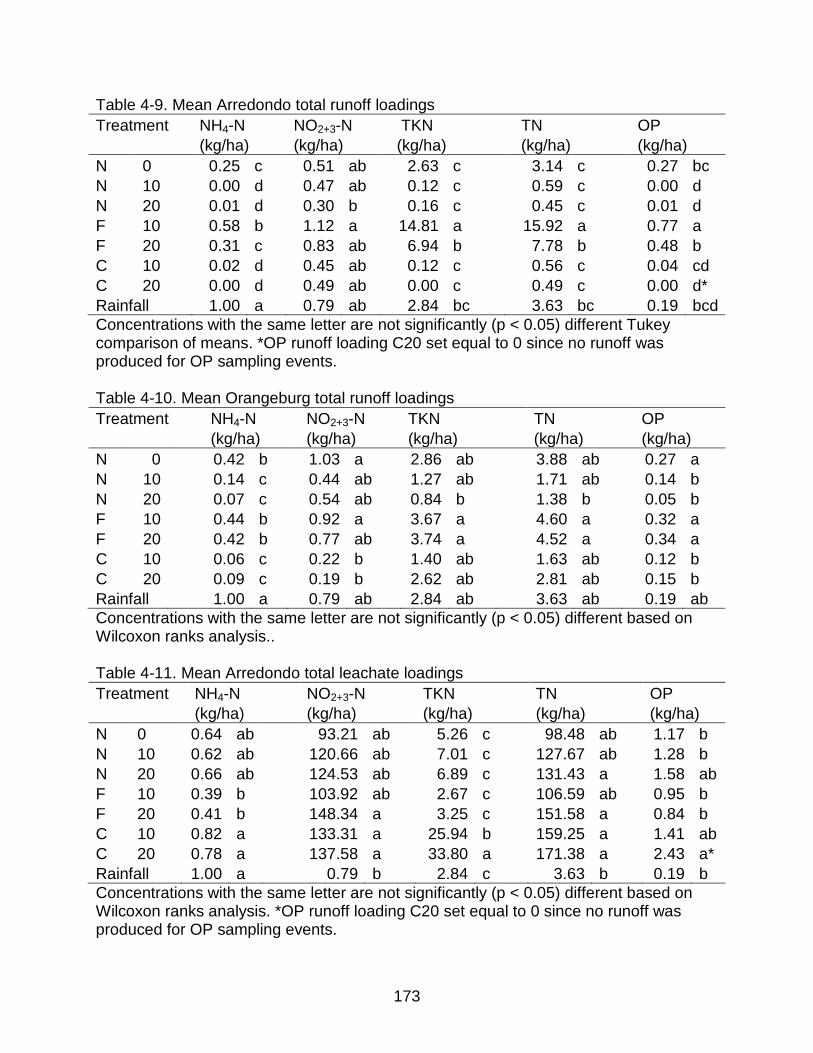
173
Table 4-9. Mean Arredondo total runoff loadings Treatment NH4-N NO2+3-N TKN TN OP
(kg/ha) (kg/ha) (kg/ha) (kg/ha) (kg/ha)
N 0 0.25 c 0.51 ab 2.63 c 3.14 c 0.27 bc N 10 0.00 d 0.47 ab 0.12 c 0.59 c 0.00 d N 20 0.01 d 0.30 b 0.16 c 0.45 c 0.01 d F 10 0.58 b 1.12 a 14.81 a 15.92 a 0.77 a F 20 0.31 c 0.83 ab 6.94 b 7.78 b 0.48 b C 10 0.02 d 0.45 ab 0.12 c 0.56 c 0.04 cd C 20 0.00 d 0.49 ab 0.00 c 0.49 c 0.00 d* Rainfall 1.00 a 0.79 ab 2.84 bc 3.63 bc 0.19 bcd Concentrations with the same letter are not significantly (p < 0.05) different Tukey comparison of means. *OP runoff loading C20 set equal to 0 since no runoff was produced for OP sampling events. Table 4-10. Mean Orangeburg total runoff loadings Treatment NH4-N NO2+3-N TKN TN OP
(kg/ha) (kg/ha) (kg/ha) (kg/ha) (kg/ha)
N 0 0.42 b 1.03 a 2.86 ab 3.88 ab 0.27 a N 10 0.14 c 0.44 ab 1.27 ab 1.71 ab 0.14 b N 20 0.07 c 0.54 ab 0.84 b 1.38 b 0.05 b F 10 0.44 b 0.92 a 3.67 a 4.60 a 0.32 a F 20 0.42 b 0.77 ab 3.74 a 4.52 a 0.34 a C 10 0.06 c 0.22 b 1.40 ab 1.63 ab 0.12 b C 20 0.09 c 0.19 b 2.62 ab 2.81 ab 0.15 b Rainfall 1.00 a 0.79 ab 2.84 ab 3.63 ab 0.19 ab Concentrations with the same letter are not significantly (p < 0.05) different based on Wilcoxon ranks analysis.. Table 4-11. Mean Arredondo total leachate loadings Treatment NH4-N NO2+3-N TKN TN OP
(kg/ha) (kg/ha) (kg/ha) (kg/ha) (kg/ha)
N 0 0.64 ab 93.21 ab 5.26 c 98.48 ab 1.17 b N 10 0.62 ab 120.66 ab 7.01 c 127.67 ab 1.28 b N 20 0.66 ab 124.53 ab 6.89 c 131.43 a 1.58 ab F 10 0.39 b 103.92 ab 2.67 c 106.59 ab 0.95 b F 20 0.41 b 148.34 a 3.25 c 151.58 a 0.84 b C 10 0.82 a 133.31 a 25.94 b 159.25 a 1.41 ab C 20 0.78 a 137.58 a 33.80 a 171.38 a 2.43 a* Rainfall 1.00 a 0.79 b 2.84 c 3.63 b 0.19 b Concentrations with the same letter are not significantly (p < 0.05) different based on Wilcoxon ranks analysis. *OP runoff loading C20 set equal to 0 since no runoff was produced for OP sampling events.
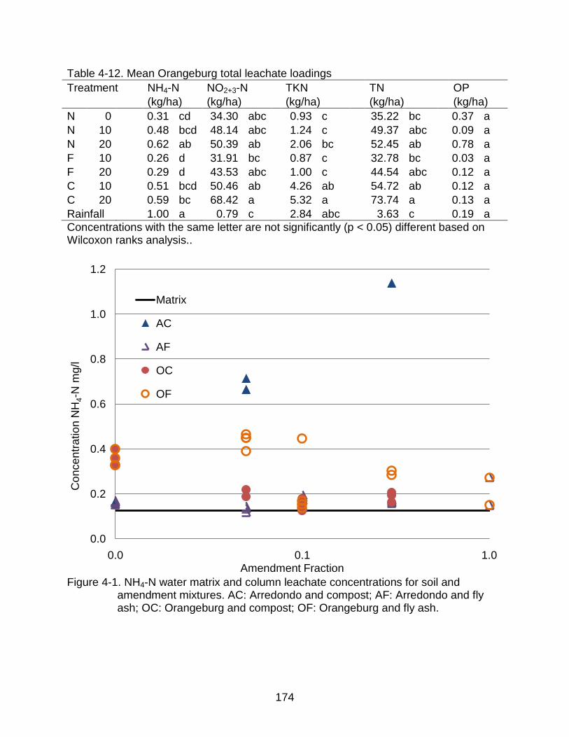
174
Table 4-12. Mean Orangeburg total leachate loadings Treatment NH4-N NO2+3-N TKN TN OP
(kg/ha) (kg/ha) (kg/ha) (kg/ha) (kg/ha)
N 0 0.31 cd 34.30 abc 0.93 c 35.22 bc 0.37 a N 10 0.48 bcd 48.14 abc 1.24 c 49.37 abc 0.09 a N 20 0.62 ab 50.39 ab 2.06 bc 52.45 ab 0.78 a F 10 0.26 d 31.91 bc 0.87 c 32.78 bc 0.03 a F 20 0.29 d 43.53 abc 1.00 c 44.54 abc 0.12 a C 10 0.51 bcd 50.46 ab 4.26 ab 54.72 ab 0.12 a C 20 0.59 bc 68.42 a 5.32 a 73.74 a 0.13 a Rainfall 1.00 a 0.79 c 2.84 abc 3.63 c 0.19 a Concentrations with the same letter are not significantly (p < 0.05) different based on Wilcoxon ranks analysis..
Figure 4-1. NH4-N water matrix and column leachate concentrations for soil and
amendment mixtures. AC: Arredondo and compost; AF: Arredondo and fly ash; OC: Orangeburg and compost; OF: Orangeburg and fly ash.
0.0
0.2
0.4
0.6
0.8
1.0
1.2
0.0 0.1 1.0
Con
cent
ratio
n N
H4-
N m
g/l
Amendment Fraction
Matrix
AC
AF
OC
OF

175
Figure 4-2. NO2+3-N water matrix and column leachate concentrations for soil and
amendment mixtures. AC: Arredondo and compost; AF: Arredondo and fly ash; OC: Orangeburg and compost; OF: Orangeburg and fly ash.
Figure 4-3. TKN water matrix and column leachate concentrations for soil and
amendment mixtures. AC: Arredondo and compost; AF: Arredondo and fly ash; OC: Orangeburg and compost; OF: Orangeburg and fly ash.
0
5
10
15
20
25
30
0.0 0.1 1.0
Con
cent
ratio
n N
O3-
N m
g/l
Amendment Fraction
MatrixACAFOCOF
0
5
10
15
20
25
30
0.0 0.1 1.0
Con
cent
ratio
n TK
N m
g/l
Amendment Fraction
MatrixACAFOCOF

176
Figure 4-4. ON water matrix and column leachate concentrations for soil and
amendment mixtures. AC: Arredondo and compost; AF: Arredondo and fly ash; OC: Orangeburg and compost; OF: Orangeburg and fly ash.
Figure 4-5. TN water matrix and column leachate concentrations for soil and
amendment mixtures. AC: Arredondo and compost; AF: Arredondo and fly ash; OC: Orangeburg and compost; OF: Orangeburg and fly ash.
0.0
5.0
10.0
15.0
20.0
25.0
30.0
0.0 0.1 1.0
Con
cent
ratio
n O
N m
g/l
Amendment Fraction
MatrixACAFOCOF
0
5
10
15
20
25
30
35
0.0 0.1 1.0
Con
cent
ratio
n TN
mg/
l
Amendment Fraction
MatrixACAFOCOF
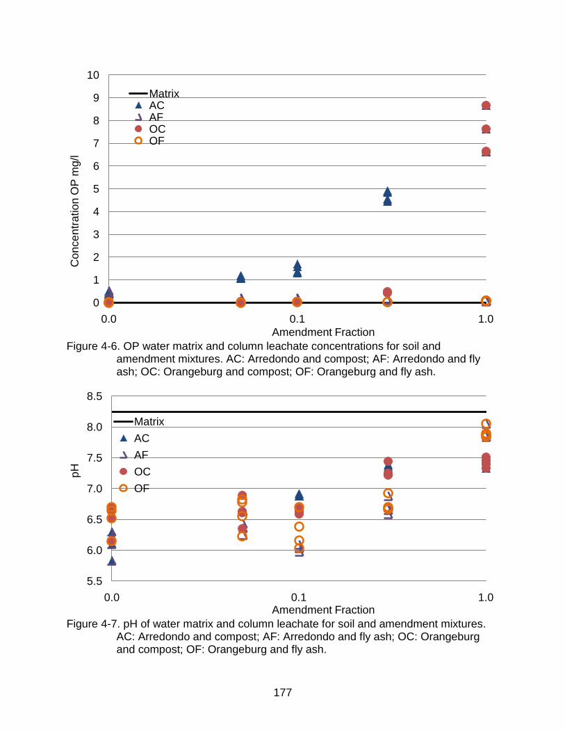
177
Figure 4-6. OP water matrix and column leachate concentrations for soil and
amendment mixtures. AC: Arredondo and compost; AF: Arredondo and fly ash; OC: Orangeburg and compost; OF: Orangeburg and fly ash.
Figure 4-7. pH of water matrix and column leachate for soil and amendment mixtures.
AC: Arredondo and compost; AF: Arredondo and fly ash; OC: Orangeburg and compost; OF: Orangeburg and fly ash.
0
1
2
3
4
5
6
7
8
9
10
0.0 0.1 1.0
Con
cent
ratio
n O
P m
g/l
Amendment Fraction
MatrixACAFOCOF
5.5
6.0
6.5
7.0
7.5
8.0
8.5
0.0 0.1 1.0
pH
Amendment Fraction
MatrixACAFOCOF
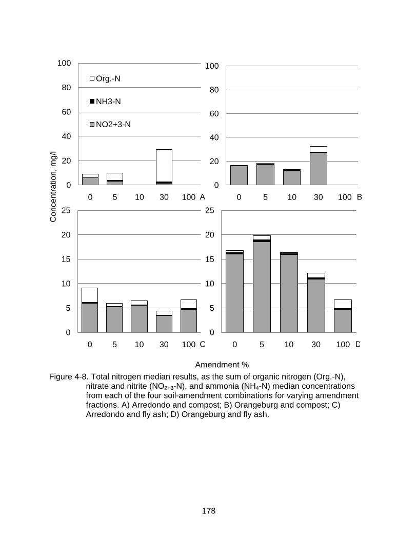
178
Figure 4-8. Total nitrogen median results, as the sum of organic nitrogen (Org.-N),
nitrate and nitrite (NO2+3-N), and ammonia (NH4-N) median concentrations from each of the four soil-amendment combinations for varying amendment fractions. A) Arredondo and compost; B) Orangeburg and compost; C) Arredondo and fly ash; D) Orangeburg and fly ash.
0
20
40
60
80
100
0 5 10 30 100
Org.-N
NH3-N
NO2+3-N
0
20
40
60
80
100
0 5 10 30 100
0
5
10
15
20
25
0 5 10 30 1000
5
10
15
20
25
0 5 10 30 100
Amendment %
Con
cent
ratio
n, m
g/l
A B
C D

179
CHAPTER 5 CONCLUSIONS
Retention Basins
Performance Conclusions
Retention (or infiltration) basins are commonly incorporated into the landscape
since retention basins primarily infiltrate stormwater on site. Captured stormwater is
eliminated primarily by infiltration which prevents contamination of downstream water
resources. However, reduced infiltration of the capture volume can reduce basin
capture volumes for subsequent runoff events, potentially allowing stormwater to
bypass treatment or elimination. To evaluate hydrologic performance of retention
basins, this study investigated infiltration rates and soil properties within 40 retention
basins in Florida, ranging in age from 0 to 20 years. Basins were equally divided
between Florida Department of Transportation (DOT) and residential land uses, while
basin soil textures ranged from sand to sandy clay. These data were complemented by
hourly water level monitoring at 11 of the basins.
The analysis in Chapter 2 showed that infiltration rates measured by Double Ring
Infiltrometer (DRI) were lower in 16 basins and higher in 14 basins, compared to design
values, while rates from the remaining basins were not different. Based on these
results, drawdown rates for 40% of the basins were at least limited by surface soil
conditions, which may have resulted from clogging, compaction, or a combination of
these two. A higher proportion of DOT basins than residential basins had DRI rates
greater than their design rates. Newer DOT basins were more likely to have significantly
greater infiltration rates than design as compared to older basins. While older DOT
basins still had greater DRI rates, the difference between DRI and design rates was

180
diminished compared to newer DOT basins. Comparably, new residential basin DRI
rates were significantly less than design. However, residential DRI rates were closer to
designs for older basins.
Increased size and diversity of vegetation as a result of less frequent maintenance
was also theorized as a potential cause of improved infiltration within DOT basins
compared to residential basins. It would be expected that basins would have improved
their performance with time as vegetation increased, however DOT basin performance
decreased with time. This indicates that other factors (i.e. changes in construction
methods with time, variable sediment loading rates), in addition to vegetation, may have
equal or greater influence on how basins perform as they age. Future research should
seek to identify these factors and determine their effects on basin performance. Basin
soil texture also affected DRI rates. Coarse textured basins had a higher proportion of
basins with DRI rates greater than their designs. Similarly, finer textured basins had a
higher proportion of basins with DRI rates below their design. This may indicate that
current basin design methods are inadequate for determining long term performance.
Furthermore, allowing for greater infiltration rates for coarse textured basins would
decrease basin surface areas could accelerate clogging and/or create groundwater
mounding that inhibits drawdown. Therefore, it is recommended that retention basin
designs account for groundwater influence on basin performance by incorporating water
table fluctuations into continuous simulation models. Basin monitoring data showed that
basin infiltration rates could also be controlled by subsurface hydrology. Of the 8
monitored basins with sufficient data, six had monitored rates less than DRI rates.
Monitored rates from the remaining two basins were not different. As a result, reduced

181
storage volume recovery in retention basins may result from reduced infiltration either
through surface soils or due to subsurface controlling conditions. Therefore,
maintenance measures aimed at improving infiltration through surface soils may not
improve storage volume recovery if subsurface hydrology is controlling infiltration.
Since infiltration rate measurement can be time and resource intensive, nine
models were evaluated to estimate DRI rates from basin soil data. The Kozeny-Carman
model incorporating porosity and harmonic mean particle diameter accurately estimated
DRI rates. Using half the inputs, the simpler MLR (2) had only slightly greater variability
than the more complex MLR (1). This result indicates that simpler models may be as
effective as more complex models for estimating DRI rates in basins. While making
evaluations based solely on model results may not be expected, modeling could be
used as an initial evaluation of whether future monitoring should occur.
Recommendations and Future Research
While vegetation was not directly measured in this study, DOT basins are typically
maintained less frequently. The increased vegetation size and variety may enhance
infiltration through soils at the basin surface. Future research of stormwater infiltration
structures should include analysis of vegetation diversity and abundance in addition to
soil characteristics. Furthermore, the presence of soil biota may also enhance soil
infiltration and should also be considered.
The hydraulics of retention basins are not only vertical, but horizontal due to lateral
seepage flow. Lateral flow can be a significant flow path for storage volume recovery,
but was not considered in this study. A supplemental study focusing on groundwater
fluctuations and lateral flow from basins would contribute to understanding retention
basins performance more thoroughly.

182
Soil Amendments
Previous research by Gregory et al. (2006) and Pitt et al. (1999) demonstrated the
impacts of urban soil compaction on decreased infiltration rates. A lysimeter research
study presented in Chapters 3 and 4 investigated the respective hydrologic and water
quality effects of amending compacted sandy (Arredondo) and sandy clay loam
(Orangeburg) soils found in Florida. Six amendment treatments were applied to each
soil, combining an amendment (compost, fly ash, or no amendment (null)) and
incorporation depths of 10 or 20 cm. Amendment treatments were compared to soils
which remained compacted.
Hydrologic Conclusions
Lysimeter soil compaction produced runoff volumes equal to or greater than
expected from “dirt roads”, according to the curve number methodology. Arredondo
soils were compacted at least to bulk densities reported for compacted Florida sands.
Orangeburg soils were compacted by the same procedure. However, insufficient
compaction of subsurface soils produced greater infiltration rates and lower measures
of soil strength than those reported for compacted sandy soils in Florida.
Amendment phase
Fly ash treatments decreased bulk densities for both soils compared to the
respective controls. However, fly ash treatments also either produced equal or greater
runoff coefficients and curve numbers due to equal or decreased infiltration rates. These
effects were attributed to the cementitious properties of fly ash which functioned to seal
soil surfaces and allowed comparatively little infiltration. Therefore it is recommended to
avoid fly ash as a soil amendment for soil compaction mitigation.

183
Null and compost treatments had greater infiltration rates and reduced runoff
production compared to the compacted lysimeters for both soils. Compost treatments
had significantly lower bulk densities than the control lysimeters. While null
incorporation mean bulk densities were lower than the control, differences were not
significant except for the 10 cm null incorporations on Orangeburg soils. Curve numbers
were not significantly different between null and compost treatments for each soil.
Though infiltration rates were greater for deeper incorporations, depth did not
generally affect Curve Numbers for treatments. Thus, shallower incorporations
produced the same benefit as deeper incorporations. While this may have resulted from
insufficient subsoil compaction, it may also suggest that the increasing incorporation
depths may not further reduce runoff production.
Applications
To quantify the potential runoff reduction of 10 cm tillage without amendments
runoff depths were calculated using the Curve Number method (NRCS 1986) and
values determined in this study for a hypothetical residential watershed. For a 2-yr 24-
hour rainfall event for Gainesville, FL (9.2 cm; Eaglin 1996) runoff depths were
approximately 3/4 and 2/3 of the runoff depth of the non-treated watershed for
Arredondo and Orangeburg soils.
In addition, runoff increases over undisturbed areas were much lower for the
amended simulated watersheds compared to non-amended simulated watersheds. Due
to greater pre-developed runoff depths, tillage reduced the expected runoff increase
more on Orangeburg soils than Arredondo soils. Therefore, soil amending may provide
greater benefits on native soils with lower infiltration rates. Furthermore, soil amending
could also offset the costs of conventional stormwater structures by reducing their size.

184
In addition, the reduced size of a retention basin would increase the available are for
development, which could be the more valuable benefit.
Water Quality Conclusions
Total nitrogen in runoff was dominated by TKN, while NO2+3-N dominated leachate
TN. Arredondo lysimeters had greater TKN, and NO2+3-N leachate concentrations than
Orangeburg lysimeters for all treatments. In addition, all Arredondo treatments had
median leachate NO2+3-N concentrations greater than the MCL of 10 mg NO2+3-N/l.
However, this was due to elevated initial concentrations which diminished below the
MCL after three months. In addition, leachate NO2+3-N loadings were not significantly
affected by treatments while significant differences between Orangeburg treatment
leachate NO2+3-N loadings were attributed to leachate volume differences. Thus,
treatments applied to Arredondo soils may be less likely to adversely affect groundwater
compared to pre-amended conditions. Orangeburg lysimeters tended to have leachate
OP concentrations less than rainfall while Arredondo leachate OP concentrations were
greater than rainfall. Thus, Orangeburg soils functioned as a sink for OP, while
Arredondo soils functioned as a source. Therefore, amending Orangeburg soils would
be less likely to increase OP loadings than Arredondo soils.
Differences between treatment runoff and leachate nutrient loadings were primarily
determined by differences of runoff and infiltration volumes rather than concentrations.
Though compost increased TKN and OP runoff concentrations over null incorporations
for Orangeburg and Arredondo lysimeters, respectively, runoff loadings were not
different. Compost treatments increased leachate TKN concentrations on both soils,
however NO2+3-N concentrations were generally not affected. Increasing incorporation
depth from 10 to 20 cm also generally did not affect runoff water quality for any of the

185
amendments. Fly ash produced equal or greater TN and OP loadings from both
Arredondo and Orangeburg soils as a result of increased runoff TKN concentrations
from Arredondo soils, coupled with increased runoff by fly ash treatments on both soils.
Annual recommended nitrogen fertilizer applications for Florida range between
100 and 150 kg N/ha (Sartain 2007). By comparison, NO2+3-N concentrations ranged
from 93 to 148 kg/ha over only four months. Though treatments did not significantly
increase Arredondo leachate TN loadings, leachate NO2+3-N loadings from both soils
were one to three orders of magnitude greater than runoff loadings. In addition, compost
treatments increased NO2+3-N loadings in leachate compared to controls due to
increased infiltration volumes and leachate concentrations. Thus leachate loadings
should not be ignored when considering water quality impacts of treatments considered
in this study. While differences in runoff volumes controlled runoff loadings, similarly,
infiltration differences generally determined leachate nutrient loadings. Impacts to
groundwater quality are often not considered when accounting for nutrient reductions to
surface waters.
Recommendations and Future Research
Fly ash incorporation was not determined to decrease runoff volumes compared to
the compacted state for either soil. However 20 cm incorporations on Orangeburg soils
significantly increased infiltration rates, due in combination to the low infiltration rate on
the compacted soils and the reduced fly ash fraction within the amended layer
compared to the 10 cm depth. In addition, due to greater nutrient concentrations and
equal or greater runoff production, fly ash produced equal or greater runoff nutrient
loadings. Therefore, fly ash should be avoided as an amendment for mitigating soil
compaction.

186
Soil compaction can occur at depths too deep to address with conventional
methods. In compacted native profiles, 10 or 20 cm amendment depths would not likely
meet or surpass the most limiting layer depths, which were found by Gregory et al.
(2006) to be deeper than 25 cm. Limiting layer depths can exceed 40 cm on
construction sites (Randrup and Lichter 2001). Therefore deeper incorporation depths
(20 cm) would be expected to further improve infiltration and reduce runoff compared to
10 cm depths. However, due to non-representative subsoil compaction in this study,
runoff reduction may not be as great on compacted in situ soils. Null and compost
treatments also decreased the bulk densities which increased the porosity of the null
and compost treatments and increased infiltration rates. As incorporation depth
increases, the additional benefits eventually diminish to negligible, regardless of the
infiltration rate due to the storage capacity of the soil. If incorporated depths do not
exceed the most limiting depth of compaction, the available water storage above the
limiting layer is increased. In this way, the amended soil functions similarly to permeable
pavement systems, where the surface layers are not limiting to infiltration, rainfall and
runoff are captured and stored and then infiltrated much more slowly. Thus, runoff may
be significantly reduced, especially from smaller rainfall events.
Null and compost incorporations were found to reduce runoff volumes and nutrient
runoff loadings from compacted soils. However, compost treatments increased NO2+3-N
leachate loading rates, which could adversely affect groundwater quality. Increasing
incorporation depths from 10 to 20 cm generally did not affect hydrologic and water
quality outcomes. Applicability of compost and null (or tillage) treatments should be

187
investigated at the plot or watershed scale to more accurately determine the real world
effects of implementing these treatments.
Future studies should directly measure leaching volumes and loadings. Ideally, a
nutrient balance would be determined to account for nutrient transport and
transformations. Additional research should investigate whether the benefits of
treatments extend to a larger scale at either the watershed or plot level. Findings from
such study would hopefully quantify the hydrologic effects of treatments more
accurately, especially with native soils below the amendment layer. While similar results
would be expected at the watershed scale, treatment effects would not expect to be as
large due to the absence of representative subsoil conditions in this study. However,
results here have shown there is a potential to reduce runoff by tilling soil, with or
without compost, down to at least 10 cm. For compacted profiles with limiting layers
below the incorporation depth, deeper incorporations would be expected to improve
hydrologic response, especially for larger events.
In addition, this study did not allow for vegetation establishment. Therefore future
research should investigate the potential water quality impacts with vegetation,
specifically with respect to leaching of nutrients which could be reduced by plant uptake.
Studies would ideally extend through multiple seasons to identify fluctuations in
hydrologic and water quality processes.

188
APPENDIX A RETENTION BASIN DATA
Table A-1. Comparison of stormwater retention design criteria for Water Management Districts (WMD) in Florida.
Design Parameter
St. Johns River WMD
Suwannee River WMD
Southwest Florida WMD
South Florida WMD
Northwest Florida WMD*
Treatment Volume
Off-line retention of the first 0.5" of runoff or 1.25" of runoff from the impervious area; whichever is greater
Retention of the runoff from the first 1" of rainfall
On-line retention of the runoff from 1" of rainfall.
Retention of the first 0.5" of runoff of 1.25" times the percentage of imperviousness; whichever is greater
Off-line retention of the first 0.5" of runoff
On-line retention of the first 1" of runoff, or 1.25" of runoff from the impervious area plus 0.5" of runoff from entire basin; whichever is greater.
If project discharges to sink, then off-line or on-line retention of the runoff from the first 2" of rainfall.
If project <100 ac, on-line retention of 0.5" of runoff.
On-line retention of the runoff from 1" of rainfall. Minimum volume of 0.5" of runoff is required.
On-line retention that percolates the runoff from the 3-year/1-hour storm
Off-line retention of runoff from 1" of rainfall
*Reproduced from Harper and Baker (2007) and updated from NWFWMD ERP Handbook II for NWFWMD criteria.

189
Table A-1. Continued. Design Parameter
St. Johns River WMD
Suwannee River WMD
Southwest Florida WMD
South Florida WMD
Northwest Florida WMD
Treatment Volume
For projects with <40% impervious and only HSG A soils, on-line retention from 1" of rainfall or 1.25" of runoff from impervious area
If project <100 ac, off-line retention of 0.5" of runoff
Volume Recovery
Provide design capacity in 72 hours using percolation, evaporation, or evapo-transpiration.
Provide design capacity in 72 hours using percolation, evaporation, or evapo-transpiration
Treatment volume recovered in < 72 hours
No more than half of treatment volume in 24 hours.
< 72 hours following storm using percolation, evaporation, or evapo-transpiration

190
Table A-2. Basin number, county location, land use, age, and design infiltration rates. Basin County (FL) Land
Age (years)# Design Infiltration Rate (cm/h)
1 Alachua DOT 16 3.56 2 Alachua Res 1 7.87 3 Alachua Res 4 8.57 4 Alachua DOT 19 21.59 5 Alachua DOT 6 4.06 6 Alachua Res 9 2.54 7 Alachua DOT 13 12.70 8 Alachua Res 11 5.08 9 Alachua DOT 18 1.52
10 Alachua Res 18 7.62 11 Alachua Res 4 2.79 12 Alachua Res 11 5.79 13 Alachua Res 13 12.80 14 Alachua Res 3 12.70 15 Alachua Res 1 6.35 16 Alachua Res 4 5.72 17 Marion DOT 13 1.52 18 Marion DOT 16 11.01 19 Marion DOT 3 5.93 20 Marion DOT 14 4.45 21 Leon Res 5 12.34 22 Leon Res 1 4.06 23 Leon Res 2 0.51 24 Leon Res 2 0.76 25 Leon Res 2 43.69 26 Leon Res 2 5.08 27 Leon Res 2 2.29 28 Leon Res 9 1.14 29 Leon Res 19 5.08 30 Leon DOT 10 12.70 31 Leon DOT 10 12.70 32 Leon DOT 6 3.18 33 Leon DOT 10 12.70 34 Leon DOT 10 12.70 35 Leon DOT 6 2.03 36 Leon DOT 3 0.33 37 Leon DOT 3 0.33 38 Leon DOT 3 0.33 39 Leon DOT 3 0.33 40 Leon DOT 6 3.18
*DOT: Department of Transportation; Res: Residential. #Age in 2008.

191
Table A-3. Soil textures for each basin test location and corresponding median basin texture.
Site Basin Median 1 2 3 4 5 6 7 8 9
1 SL SL* C SL SL SCL SCL LS S SL 2 LS LS LS LS LS SCL S LS S S 3# S S
4 SL L SL S LS L S 5 SL SL SL SL SL SL SL 6 SCL C SL SCL C SCL SC 7 S LS SL S S S S 8 SL SL SL SL L SL SL 9 SC HC HC SC SCL SCL SC 10 S S SCL S S S S 11 SL SC SL SL SL SL SL 12 LS S S LS SCL LS LS 13 LS SL LS SL LS LS SCL 14 S S S S S S LS 15 SCL SCL SC SCL SCL SCL SL 16 S S S S S S S 17 S S S LS S S LS 18 LS S S LS LS LS LS 19 S S S S S S S 20 S S S S LS S S 21 SL SCL SL SL SL SL SL 22 SL SCL SL SCL SL SCL SL 23 SL SL SL SL SL SL SL 24 SCL SCL SCL SCL SCL SCL SC 25 S S S S S S S 26 LS LS LS LS SL LS SCL 27 SL SCL LS LS SL SL SCL 28 SCL SCL SCL SL SC C SCL 29 SCL SCL SCL C
30 SCL SL SCL SCL SCL SCL SCL 31 SCL SCL HC SC SCL SCL SCL 32 S S S S S S S 33 SCL SCL SL SL SCL SCL SCL 34 SCL SCL SCL SL SCL SCL SC 35 S S S S LS S S 36 SCL L SCL SCL SCL SCL LS 37 LS LS LS LS LS SL SL 38 SL LS SL SL LS SL SL 39 LS LS LS LS SL LS LS 40 S S S S S S S *S: Sand; LS: Loamy Sand; SL: Sandy Loam; SCL: Sandy Clay Loam; SC: Sandy Clay;
L: Loam; C: Clay; HC: Heavy Clay. #Limited site access prevented additional soil sample collection.
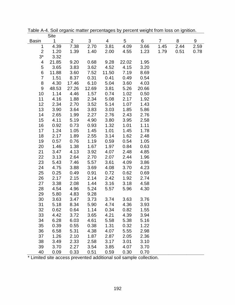
192
Table A-4. Soil organic matter percentages by percent weight from loss on ignition.
Basin Site
1 2 3 4 5 6 7 8 9 1 4.39 7.38 2.70 3.81 4.09 3.66 1.45 2.44 2.59 2 1.20 1.39 1.40 2.00 4.55 1.23 1.79 0.51 0.78
3* 3.32 4 21.85 9.20 0.68 9.28 22.02 1.95
5 3.65 3.83 3.62 4.52 4.15 3.20 6 11.88 3.60 7.52 11.50 7.19 8.69 7 1.51 8.37 0.31 0.41 0.49 0.54 8 4.30 17.46 6.10 5.04 3.60 4.03 9 48.53 27.26 12.69 3.81 5.26 20.66 10 1.14 4.46 1.57 0.74 1.02 0.50 11 4.16 1.88 2.34 5.08 2.17 1.92 12 2.34 2.70 3.52 5.14 1.07 1.43 13 3.90 3.64 3.83 3.03 1.85 5.86 14 2.65 1.99 2.27 2.76 2.43 2.76 15 4.11 5.19 4.90 3.80 3.95 2.58 16 0.92 0.73 0.93 1.32 1.01 1.11 17 1.24 1.05 1.45 1.01 1.45 1.78 18 2.17 1.89 2.55 3.14 1.62 2.48 19 0.57 0.76 1.19 0.59 0.54 1.05 20 1.46 1.38 1.67 1.97 0.84 0.63 21 3.47 4.13 3.92 4.07 2.48 4.85 22 3.13 2.64 2.70 2.07 2.44 1.96 23 5.43 7.46 5.57 3.61 4.09 3.86 24 4.75 3.88 3.69 4.08 3.70 4.23 25 0.25 0.49 0.91 0.72 0.62 0.69 26 2.17 2.15 2.14 2.42 1.92 2.74 27 3.38 2.08 1.44 3.16 3.18 4.58 28 4.54 4.96 5.24 5.57 5.96 4.30 29 5.80 4.83 9.28
30 3.63 3.47 3.73 3.74 3.63 3.76 31 5.18 8.34 5.90 4.74 4.36 3.93 32 0.62 0.64 1.14 0.34 0.82 1.55 33 4.42 3.72 3.65 4.21 4.39 3.94 34 6.28 6.03 4.61 5.58 5.38 5.16 35 0.39 0.55 0.38 1.31 0.32 1.22 36 6.58 5.31 4.38 4.07 5.55 2.98 37 1.26 2.10 1.87 2.87 2.05 2.36 38 3.49 2.33 2.58 3.17 3.01 3.10 39 3.70 2.27 3.54 3.85 4.07 3.70 40 0.09 0.33 0.51 0.59 0.30 0.70 * Limited site access prevented additional soil sample collection.

193
Table A-5. Bulk density (g/cm3) measurements from each basin location. Site Basin 1 2 3 4 5 6 7 8 9
1 1.57 1.18 1.60 1.60 1.41 1.56 1.65 1.61 1.49 2 1.65 1.79 1.67 1.74 1.80 1.72 1.77 1.58 1.68
3* 1.37 4 0.66 0.97 1.67 1.24 0.62 1.40 5 1.44 1.50 1.58 1.43 1.38 1.64 6 0.99 1.43 1.10 1.01 1.33 1.26 7 1.67 1.21 1.55 1.62 1.58 1.63 8 1.38 0.91 1.36 1.58 1.47 1.53 9 0.23 0.46 0.84 1.35 1.21 0.54
10 1.53 1.55 1.35 1.64 1.58 1.61 11 1.48 1.67 1.58 1.45 1.65 1.63 12 1.55 1.54 1.51 1.40 1.27 1.64 13 1.44 1.54 1.52 1.57 1.62 1.13 14 1.22 1.44 1.49 1.45 1.57 1.46 15 1.57 1.57 1.42 1.41 1.61 1.72 16 1.54 1.59 1.50 1.53 1.61 1.56 17 1.64 1.58 1.76 1.66 1.65 1.72 18 1.49 1.51 1.31 1.41 1.52 1.53 19 1.62 1.58 1.55 1.61 1.64 1.65 20 1.65 1.64 1.66 1.69 1.73 1.63 21 1.70 1.47 1.63 1.59 1.62 1.43 22 1.78 1.71 1.78 1.67 1.73 1.73 23 1.51 1.54 1.37 1.41 1.75 1.57 24 1.63 1.78 1.71 1.61 1.82 1.64 25 1.54 1.61 1.61 1.58 1.63 1.56 26 1.61 1.50 1.44 1.45 1.54 1.41 27 1.78 1.54 1.81 1.69 1.74 1.77 28 1.61 1.56 1.46 1.34 1.50 1.37 29 1.41 1.65 1.34 30 1.39 1.66 1.67 1.60 1.67 1.61 31 1.49 1.36 1.51 1.64 1.61 1.42 32 1.68 1.63 1.66 1.67 1.52 1.55 33 1.51 1.46 1.65 1.58 1.59 1.59 34 1.36 1.34 1.44 1.42 1.43 1.59 35 1.63 1.70 1.61 1.69 1.68 1.70 36 1.40 1.30 1.42 1.47 1.42 1.56 37 1.67 1.55 1.61 1.61 1.71 1.63 38 1.54 1.63 1.50 1.64 1.71 1.52 39 1.36 1.62 1.58 1.59 1.63 1.54 40 1.58 1.42 1.60 1.59 1.56 1.60
* Limited site access prevented additional soil sample collection.

194
Table A-6. Measured double ring infiltrometer infiltration rates (cm/h) for each basin test location.
Site Basin 1 2 3 4 5 6 7 8 9
1 0.01 0.96 0.24 0.82 1.50 0.92 1.94 5.96 0.58 2 1.20 0.87 0.20 0.01 0.01 3.38 0.01 1.33 7.37 3 6.93 13.82 9.66 15.59 23.56 14.65 4 58.20 36.40 37.34 27.03 56.15 96.00 5 0.39 0.23 0.37 0.39 0.09 1.33 6 1.04 3.55 0.67 0.20 0.48 0.55 7 8.06 4.98 56.89 22.65 43.91 17.56 8 5.08 2.22 3.66 0.40 6.24 0.55 9 252.00 108.00 18.00 5.53 112.89 109.08
10 14.39 122.84 18.09 38.87 25.41 41.39 11 0.46 1.11 1.54 1.04 1.39 1.37 12 9.60 9.95 10.37 33.81 23.56 10.43 13 4.12 4.98 2.30 1.85 5.52 1.85 14 17.51 5.77 15.45 35.61 15.67 12.47 15 0.28 0.40 0.13 0.69 0.58 0.25 16 28.55 18.08 13.86 12.38 20.05 8.31 17 35.05 27.12 4.48 29.11 28.34 17.55 18 10.83 7.48 12.47 27.05 18.52 26.05 19 19.41 16.63 34.31 22.08 20.74 22.18 20 3.88 13.56 22.01 18.66 12.42 18.01 21 0.26 4.73 0.39 0.69 4.16 0.01 22 0.13 2.77 0.46 4.15 0.43 2.42 23 1.19 0.92 0.92 3.04 0.01 0.14 24 0.39 0.39 0.31 0.31 0.46 0.39 25 19.40 41.66 23.19 24.40 17.51 50.62 26 1.11 2.22 2.76 1.11 4.74 0.08 27 1.11 1.58 0.55 4.69 1.98 1.57 28 0.22 0.83 1.04 0.20 1.38 0.92 29 0.12 0.74 0.01 30 1.66 1.39 0.13 0.28 3.31 0.92 31 1.66 1.10 1.18 0.91 1.66 0.83 32 27.64 15.94 5.91 33.24 15.71 28.11 33 4.16 5.52 0.34 0.01 1.66 1.10 34 4.16 2.40 4.34 6.47 2.22 1.11 35 24.48 45.63 28.89 2.30 0.55 6.90 36 79.47 9.24 2.07 1.94 2.32 3.23 37 8.32 8.31 2.77 0.54 1.11 0.55 38 1.66 2.77 5.99 3.86 1.66 1.66 39 0.81 1.38 1.11 0.55 2.22 2.22 40 55.19 19.36 19.39 24.69 52.69 19.32

195
APPENDIX B SOIL MOISTURE AND CONE PENETROMETER DATA
Soil Moisture
Time Domain Reflectometer
A Field Scout® TDR 300 Soil Moisture Probe is a Time Domain Reflectometer
(TDR) and was used to measure volumetric water content at five locations surrounding
each infiltration measurement location. A probe with two 20 cm long rods was inserted
into the soil for this measurement. The TDR was successfully used to record 809
individual measurements at 180 locations within 36 basins (Table B1). In four basins,
soil conditions were too dry to insert the TDR probe to obtain moisture readings. Since
soil strength is dependent on moisture content, it was determined that attempting to
replace failed measurements with additional successful readings, would bias the sample
population to higher moisture contents.
Volumetric Water Content
Volumetric water contents were measured from soil samples collected from each
site. Values were determined as the difference in sample masses before and after
drying divided by the sample volume.
Figure B1 shows corresponding volumetric water content measurements from soil
samples and average TDR readings from all locations where both were collected. The
regression shows that the average TDR values were about 10% higher than the
corresponding soil sample θv values.
One explanation for this is that the soil below the soil samples had a slightly higher
VWC than the samples. Since the TDR rods extended 20 cm into the soil profile,
compared to the 10 cm of the soil sample, TDR readings would be slightly higher. This

196
difference would be expected given that evaporation dries soils from the surface down.
However, previous research in an uncompacted sandy Florida soil by Dukes et al.
(2006) showed that gravimetric samples had a slightly higher VWC when compared to
TDR readings.
Soil Strength
A Field Scout® SC 900 Soil Compaction Meter is a cone penetrometer (CP) used
to measure the pressure required at various soil depths to continuously force a cone
through a soil profile. Penetrometer profile measurements were conducted at five
locations surrounding each infiltration rate measurement. The SC 900 recorded
pressure (kPa) measurements at 2.5 cm increments (up to 45 cm) with a maximum
value of 7,000 kPa. If the CP did not reach a depth of 10 cm, data was not recorded. As
with the TDR measurements, soil moisture often seemed to determine whether a CP
soil profile data was able to be collected. Therefore, several profiles were neither
complete (45 cm) nor truncated (10 – 42.5 cm) and data was not collected. Attempting
to replace failed measurements by additional measurements could lead to bias in the
data.
The cone penetrometer (CP) was used to collect 776 soil profiles from 185 basins
in 36 basins. In an expected profile, the entire 45 cm soil profile would be measured,
where the maximum value and corresponding depths are clearly identifiable. Thus, the
maximum CP reading for a profile would likely be correlated to the infiltration rate
(Gregory et al. 2006). As mentioned previously, complete profiles were difficult to
achieve, only 81 of 776 were complete, as seen in Table B3. All other CP attempts were
truncated or not recorded.

197
Correlations between reading and depth values from the 81 complete profiles and
soil sample volumetric water content and measured infiltration rates yielded no
significant relationships across basins. The only significant (p < 0.05) depth for
correlation was at 10 cm; all other depths were not significant (p > 0.05). By
comparison, Gregory et al. (2006) reported all depths greater than 0.0 had p-values less
than 0.13, however, only three of the 18 values in this study had comparable
correlation. In addition, all Pearson’s r values for Gregory et al. (2006) were negative,
suggesting that a greater force corresponded to a decreased infiltration rate, however
for depths greater than 20 cm in the present study, Pearson’s r values are positive.

198
Table B-1. Volumetric water content by TDR attempts and successes for each basin.
Basin Attempted Success Success Rate Basin Attempted Success
Success Rate
1 45 44 0.98 21 30 29 0.97 2 55 55 1.22 22 30 24 0.80 3 0 0 0.00 23 30 30 1.00 4 30 30 1.00 24 30 25 0.83 5 36 36 1.20 25 30 29 0.97 6 30 30 1.00 26 30 0 0.00 7 30 25 0.83 27 30 0 0.00 8 30 8 0.27 28 30 9 0.30 9 31 31 1.03 29 15 15 1.00 10 31 31 1.03 30 30 30 1.00 11 30 10 0.33 31 30 0 0.00 12 30 7 0.23 32 30 22 0.73 13 30 8 0.27 33 30 4 0.13 14 30 29 0.97 34 30 1 0.03 15 30 21 0.70 35 30 30 1.00 16 30 14 0.47 36 30 2 0.07 17 30 30 1.00 37 30 1 0.03 18 30 30 1.00 38 30 0 0.00 19 30 30 1.00 39 30 30 1.00 20 30 29 0.97 40 30 30 1.00
Total 1203 809 0.67

199
Table B-2. Gravimetric volumetric water (m3/m3) content measurements from each basin location.
Site Basin 1 2 3 4 5 6 7 8 9
1 0.34 0.47 0.28 0.31 0.39 0.29 0.28 0.24 0.33 2 0.07 0.10 0.16 0.12 0.29 0.09 0.13 0.09 0.07 3 0.25 4 0.35 0.29 0.10 0.22 0.35 0.19 5 0.11 0.22 0.25 0.26 0.16 0.20 6 0.45 0.30 0.40 0.44 0.31 0.32 7 0.08 0.24 0.01 0.02 0.02 0.10 8 0.05 0.14 0.05 0.11 0.17 0.13 9 0.43 0.46 0.47 0.27 0.20 0.24
10 0.03 0.20 0.03 0.05 0.03 0.01 11 0.26 0.11 0.13 0.09 0.12 0.08 12 0.02 0.03 0.03 0.12 0.09 0.03 13 0.12 0.11 0.09 0.15 0.07 0.18 14 0.02 0.02 0.02 0.02 0.03 0.02 15 0.26 0.33 0.20 0.19 0.28 0.17 16 0.04 0.03 0.02 0.02 0.03 0.02 17 0.08 0.07 0.10 0.07 0.09 0.09 18 0.08 0.10 0.10 0.13 0.09 0.18 19 0.04 0.06 0.06 0.06 0.05 0.06 20 0.14 0.08 0.08 0.11 0.06 0.06 21 0.19 0.17 0.18 0.16 0.14 0.17 22 0.24 0.16 0.22 0.15 0.18 0.15 23 0.30 0.30 0.28 0.22 0.23 0.31 24 0.25 0.22 0.19 0.19 0.24 0.27 25 0.05 0.06 0.07 0.06 0.06 0.04 26 0.09 0.12 0.09 0.12 0.11 0.19 27 0.19 0.12 0.12 0.18 0.21 0.25 28 0.24 0.25 0.28 0.25 0.28 0.22 29 0.38 0.31 0.42 30 0.18 0.18 0.23 0.26 0.25 0.22 31 0.14 0.25 0.21 0.14 0.13 0.10 32 0.03 0.05 0.05 0.04 0.03 0.03 33 0.12 0.09 0.13 0.12 0.14 0.11 34 0.13 0.13 0.12 0.16 0.14 0.16 35 0.22 0.16 0.13 0.13 0.10 0.13 36 0.18 0.13 0.11 0.07 0.13 0.07 37 0.06 0.07 0.06 0.07 0.11 0.10 38 0.06 0.08 0.07 0.09 0.10 0.10 39 0.26 0.26 0.28 0.29 0.27 0.23 40 0.01 0.01 0.01 0.01 0.01 0.02

200
Table B-3. Summary table of attempts, complete, truncated profile measurements, and average depth of maximum reading for each basin.
Basin Potential Tests
Full Profile
Success Rate
Truncated Profile
Success Rate
Depth of Max (cm)
1 45 8 0.18 37 0.82 22.7 2 45 0 0.00 0 0.00 N/A† 3 0 0 0.00 0 0.00 N/A† 4 30 0 0.00 30 1.00 24.9 5 30 5 0.17 18 0.60 16.1 6 30 2 0.07 18 0.60 23.1 7 30 0 0.00 3 0.10 11.7 8 30 0 0.00 0 0.00 N/A† 9 30 6 0.20 24 0.80 23.3 10 30 5 0.17 26 0.87 21.8 11 30 2 0.07 3 0.10 8.5 12 30 0 0.00 9 0.30 11.1 13 30 1 0.03 10 0.33 14.5 14 30 0 0.00 16 0.53 12.2 15 30 5 0.17 19 0.63 14.0 16 30 0 0.00 28 0.93 10.5 17 30 0 0.00 30 1.00 20.0 18 30 0 0.00 31 1.03 21.8 19 30 27 0.90 3 0.10 29.2 20 30 0 0.00 30 1.00 19.2 21 30 0 0.00 28 0.93 12.7 22 30 1 0.03 19 0.63 8.1 23 30 1 0.03 29 0.97 18.8 24 30 1 0.03 21 0.70 12.8 25 30 0 0.00 30 1.00 21.8 26 30 3 0.10 27 0.90 15.3 27 30 0 0.00 20 0.67 10.1 28 30 9 0.30 15 0.50 17.2 29 15 1 0.07 14 0.93 26.5 30 30 4 0.13 25 0.83 23.7 31 30 0 0.00 1 0.03 35.0 32 30 0 0.00 26 0.87 18.9 33 30 0 0.00 2 0.07 8.8 34 30 0 0.00 2 0.07 8.8 35 30 0 0.00 28 0.93 23.2 36 30 0 0.00 5 0.17 11.0 37 30 0 0.00 0 0.00 N/A† 38 30 0 0.00 3 0.10 7.5 39 30 0 0.00 30 1.00 29.7 40 30 0 0.00 30 1.00 25.8
Total 1185 81 0.07 690 0.58 †No profiles, complete or truncated, were successfully collected at these basins.

201
Table B-4. Correlation and probability values (p) between cone penetrometer
measurements at 2.5 cm increments and measured infiltration rates in basins for full profiles.
Depth (cm) Pearson's Coefficient (r) p-value 0.0 -0.0805 0.173 2.5 0.0174 0.746 5.0 -0.1261 0.158 7.5 -0.2105 0.209
10.0 -0.3057 0.043 12.5 -0.1757 0.193 15.0 -0.1086 0.189 17.5 -0.0925 0.112 20.0 -0.1040 0.144 22.5 0.1206 0.885 25.0 0.1855 0.992 27.5 0.1871 0.547 30.0 0.2157 0.827 32.5 0.4065 0.331 35.0 0.2467 0.422 37.5 0.3026 0.224 40.0 0.2720 0.225 42.5 0.1648 0.462 45.0 0.1966 0.101

202
Figure B-1. Average TDR VWC readings vs. Gravimetric VWC for each location tested.
y = 1.10xR2 = 0.70
0
10
20
30
40
50
60
70
0 10 20 30 40 50Gravimetric VWC (m3/m3)
Aver
age
Loca
tion
TDR
VW
C (m
3 /m3 )

203
APPENDIX C MONITORING DATA
Table C-1. Summary of drawdown events for monitoring in basin 4. Soil texture: Sandy Loam. Land use: Department of Transportation.
Event Date
Rainfall Depth (cm)
Max Hourly Intensity (cm/h)
Duration (h)
Avg. Intensity (cm/h)
Max Water Level (cm)
Avg. Drawdown Rate (cm/h)
Ponded Duration (h)
03/29/09 60.8 31.6 7 0.9 270 2.28 49 04/01/09 26.6 9.6 21 0.1 147 0.84 20 04/14/09 23.0 4.8 13 0.2 145 0.94 16 04/20/09 19.8 9.0 9 0.2 157 1.24 22 05/14/09
278 3.17
05/16/09
144 1.12 16 05/17/09
128 1.05
05/18/09
146 0.95 05/18/09
155 1.38
05/20/09
224 2.14 05/21/09
194 2.34
05/22/09
222 2.88 05/23/09
167 1.30 25
05/26/09
142 0.69 22 05/28/09
146 0.66 26
06/05/09
138 0.86 20 06/06/09
118 0.20 5
06/13/09
228 1.70 50 06/16/09
158 1.22
06/17/09
178 0.91 50 06/23/09
126 0.37 12
06/30/09
213 1.68 47 07/03/09 12.4 11.6 5 0.2 133 0.60 17 07/07/09 11.8 6.4 5 0.2 129 0.95 15 07/08/09 19.2 6.0 12 0.2 162 1.29
07/09/09 2.6 2.4 2 0.1 134 0.62 16 07/10/09 30.0 20.6 4 0.8 200 1.62
07/16/09 4.4 2.8 5 0.1 125 0.41 11 07/18/09 14.8 12.0 8 0.2 143 0.72 26 07/24/09 17.0 10.4 2 0.9 148 1.34
07/25/09 7.2 5.4 2 0.4 134 0.67 15 07/30/09 41.4 39.0 5 0.8 253 2.63
07/31/09 22.0 12.4 11 0.2 234 1.88 08/02/09 8.6 8.4 3 0.3 150 1.38 22
08/03/09 13.4 13.2 2 0.7 155 1.31 08/04/09 23.0 22.4 7 0.3 228 2.20

204
Table C-1. Continued.
Event Date
Rainfall Depth (cm)
Max Hourly Intensity (cm/h)
Duration (h)
Avg. Intensity (cm/h)
Max Water Level (cm)
Avg. Drawdown Rate (cm/h)
Ponded Duration (h)
08/06/09 12.8 9.0 13 0.1 184 1.81 08/06/09 2.2 1.2 2 0.1 165 0.98 31
08/13/09 9.4 9.0 7 0.1 175 1.30 08/15/09 2.8 1.8 5 0.1 121 0.21 6
08/18/09 9.0 8.2 2 0.5 120 0.25 8 08/21/09 28.4 26.8 2 1.4 171 1.35
08/27/09 51.8 12.4 9 0.6 245 1.61 65 09/02/09 27.4 24.8 5 0.5 183 1.04 51 09/12/09 5.0 4.2 3 0.2 118 0.19 4 09/18/09 6.0 3.6 10 0.1 142 0.72 22 10/05/09 15.8 9.2 7 0.2 150 0.94 23 11/11/09 10.8 5.2 27 0.0 115 0.04 2 11/22/09 13.0 4.2 9 0.1 134 0.63 15 11/24/09 8.0 5.4 3 0.3 124 0.67
11/25/09 45.4 22.0 13 0.3 259 1.72 65 12/02/09 10.2 6.0 6 0.2 133 0.50 20 12/05/09 34.2 4.4 22 0.2 190 0.87 62 12/25/09 7.4 7.0 4 0.2 121 0.20 9 01/01/10 18.8 7.6 8 0.2 153 0.62 37 Max 60.8 39.0 27 1.4 278 3.17 65 Median 13.4 8.4 6 0.2 150 0.98 21 Min 2.2 1.2 2 0.0 115 0.04 2 Mean 18.3 10.8 8 0.3 166 1.15 26 SD 14.0 8.8 6 0.3 44 0.71 18

205
Table C-2. Summary of drawdown events for monitoring in basin 5. Soil texture: Sandy Loam. Land use: Department of Transportation.
Event Date
Rainfall Depth (cm)
Max Hourly Intensity (cm/h)
Duration (h)
Avg. Intensity (cm/h)
Max Water Level (cm)
Avg. Drawdown Rate (cm/h)
Ponded Duration (h)
03/28/09 8.78 2.94 9 0.98 36.35 0.29 70 04/03/09 1.48 1.28 5 0.30 25.41 0.23 89 04/06/09 0.10 0.04 10 0.01 6.61 0.42 14 05/20/09 0.56 0.22 5 0.11 3.18 0.44 7 05/23/09
20.86 0.37 55
05/26/09
12.22 0.44 27 05/28/09
37.62 0.54 69
06/30/09
8.29 0.26 31 07/02/09
3.26 1.24 2
07/03/09
11.03 0.37 29 07/08/09
17.89 0.41 44
07/10/09
24.90 0.49 46 07/15/09 0.66 0.04 73 0.01 16.16 0.42 35 07/25/09
18.27 0.37 47
08/25/09 2.36 2.18 7 0.34 3.54 0.22 15 08/27/09 2.46 1.16 8 0.31 18.65 0.29 17 08/28/09 1.82 0.98 4 0.46 22.28 0.38 54 12/05/09 2.76 0.44 22 0.13 3.18 0.19 16 01/01/10 2.78 1.92 10 0.28 4.43 0.18 23 Max 8.78 2.94 73 0.98 37.62 1.24 89 Median 2.09 1.07 9 0.29 16.16 0.37 31 Min 0.10 0.04 4 0.01 3.18 0.18 2 Mean 2.38 1.12 15 0.29 15.48 0.40 36 St Dev 2.45 0.98 21 0.28 10.78 0.23 24

206
Table C-3. Summary of drawdown events for monitoring in basin 6. Soil texture: Sandy Clay Loam. Land use: Residential.
Event Date
Rainfall Depth (cm)
Max Hourly Intensity (cm/h)
Duration (h)
Avg. Intensity (cm/h)
Max Water Level (cm)
Avg. Drawdown Rate (cm/h)
Ponded Duration (h)
5/24/09 2.90 0.28 102 0.03 51.53 0.24 108 5/28/09
42.46 0.23 165
6/5/09 0.86 0.18 8 0.11 9.11 0.16 59 6/30/09 0.16 0.02 29 0.01 17.29 0.19 65 7/4/09 2.06 2.02 6 0.34 16.81 0.16 82 7/8/09 1.96 0.66 22 0.09 23.13 0.16 44 7/12/09 1.76 0.44 16 0.11 35.15 0.23 53 7/14/09
25.16 0.18 51
7/16/09
18.48 0.18 105 8/7/09 1.78 0.30 22 0.08 6.65 0.15 47 8/27/09 0.28 0.14 9 0.03 2.91 0.11 10 8/29/09 0.30 0.08 24 0.01 32.68 0.18 182 9/12/09 0.96 0.14 21 0.05 1.49 0.10 17 9/19/09 4.40 2.50 10 0.44 26.56 0.18 111 9/24/09 1.58 0.70 5 0.32 11.45 0.17 70 10/16/09 2.22 1.20 11 0.20 4.87 0.11 47 12/6/09 2.84 0.44 22 0.13 7.10 0.12 63 Max 4.40 2.50 102 0.44 51.53 0.24 182 Median 1.77 0.37 19 0.10 17.29 0.17 63 Min 0.16 0.02 5 0.01 1.49 0.10 10 Average 1.72 0.65 22 0.14 19.58 0.17 75 St Dev 1.18 0.76 24 0.14 14.55 0.04 46
Table C-4. Summary of drawdown events for monitoring in basin 13. Soil texture: Loamy Sand. Land use: Residential.
Event Date
Rainfall Depth (cm)
Max Hourly Intensity (cm/h)
Duration (h)
Avg. Intensity (cm/h)
Max Water Level (cm)
Avg. Drawdown Rate (cm/h)
Ponded Duration (h)
08/06/09 5.54 2.90 2 2.77 12.81 0.54 23 09/17/09 8.38 4.72 8 1.05 10.61 0.50 21 Average 6.96 3.81 5 1.91 11.71 0.52 22 St Dev 2.01 1.29 4 1.22 1.56 0.03 1

207
Table C-5. Summary of drawdown events for monitoring in basin 18. Soil texture: Loamy Sand. Land use: Department of Transportation.
Event Date
Rainfall Depth (cm)
Max Hourly Intensity (cm/h)
Duration (hr)
Avg. Intensity (cm/h)
Avg. Drawdown Rate (cm/h)
Max Water Level (cm)
Ponded Duration
(h) 5/18/09 16.18 0.18 69 0.18 0.15 16.7
5/22/09 0.62 0.44 5 0.12 0.08 22.3 5/22/09 0.14 0.06 3 0.05 0.08 21.9 5/23/09 3.26 2.06 6 0.54 0.13 21.2 5/24/09 0.84 0.36 5 0.17 0.10 22.4 5/25/09 0.36 0.34 2 0.18 0.09 22.0 5/26/09 0.90 0.86 2 0.45 0.08 21.5 5/28/09 0.58 0.58 1 0.58 0.11 20.5 136
6/5/09 1.44 2.14 5 0.58 0.07 17.2 6/5/09 0.38 1.50 2 0.66 0.09 17.0 6/6/09 1.38 0.78 11 0.13 0.07 17.6 6/7/09 0.30 1.04 1 0.19 0.26 17.2 25
7/6/09 1.86 0.42 8 0.13 0.43 17.2 15 7/7/09 0.82 1.06 2 0.30 0.47 17.2 14 7/8/09 1.78 0.28 8 0.23 0.26 17.1
7/9/09 1.28 0.30 7 0.41 0.43 16.4 20 7/10/09 2.88 2.10 6 0.48 0.19 18.3 47 7/13/09 0.70 0.84 1 0.18 0.51 17.0 12 7/14/09 0.44 0.80 1 0.48 0.60 16.9 9 7/18/09 2.78 0.70 3 0.70 0.31 17.3 21 7/20/09 4.54 2.82 2 2.27 0.13 19.0 85 8/4/09 2.78 0.44 9 0.93 0.52 17.6 14 8/15/09 1.28 2.38 4 2.27 0.50 16.6 10 8/16/09 0.82 1.92 2 0.31 0.51 16.5 9 9/2/09 3.10 1.26 6 0.32 0.39 17.1 15 9/18/09 9.42 3.46 6 1.57 0.11 21.2 156 11/22/09 4.02 0.78 7 0.52 0.39 16.5 12 11/25/09 2.10 1.88 15 1.57 0.20 16.5 23 12/4/09 3.84 1.70 21 0.57 0.11 16.1 56 1/1/10 2.62 1.08 12 0.22 0.38 15.8 8 Max 16.18 3.46 69 2.27 0.60 22.4 156 Median 1.41 0.85 5 0.43 0.20 17.2 15 Min 0.14 0.06 1 0.05 0.07 15.8 8 Mean 2.45 1.15 8 0.58 0.26 18.3 36 St. Dev. 3.20 0.86 12 0.59 0.17 2.2 43

208
Table C-6. Summary of drawdown events for monitoring in basin 21. Soil texture: Sandy
Loam. Land use: Residential.
Event Date
Rainfall Depth (cm)
Max Hourly Intensity (cm/h)
Duration (h)
Avg. Intensity (cm/h)
Max Water Level (cm)
Avg. Drawdown Rate (cm/h)
Ponded Duration (h)
04/02/09 2.92 0.17 92 0.12 7.21 0.43 15 04/13/09 3.84 0.29 20 0.24 2.68 0.75 2 Average 3.38 0.23 56 0.18 4.94 0.59 9 St Dev 0.65 0.09 51 0.08 3.20 0.23 9
Table C-7. Summary of drawdown events for monitoring in basin 25. Soil texture: Sand.
Land use: Residential.
Event Date
Rainfall Depth (cm)
Max Hourly Intensity (cm/h)
Duration (h)
Avg. Intensity (cm/h)
Max Water Level (cm)
Avg. Drawdown Rate (cm/h)
Ponded Duration (h)
12/02/09 12.98 3.14 30 0.43 66.65 1.11 24 06/29/09 3.08 0.78 74 0.04 11.03 1.09 4 04/02/09 9.30 0.42 278 0.03 10.22 0.68 5 04/14/09 7.16 1.42 13 0.55 3.13 0.67 2 Max 12.98 3.14 278 0.55 66.65 1.11 24 Median 8.23 1.10 52 0.24 10.62 0.89 5 Min 3.08 0.42 13 0.03 3.13 0.67 2 Average 8.13 1.44 99 0.26 22.76 0.89 9 St Dev 4.14 1.21 122 0.27 29.48 0.24 10

209
Table C-8. Summary of drawdown events for monitoring in basin 30. Soil texture: Sandy Clay Loam. Land use: Department of Transportation.
Event Date
Rainfall Depth (cm)
Max Hourly Intensity (cm/h)
Duration (h)
Avg. Intensity (cm/h)
Max Water Level (cm)
Avg. Drawdown Rate (cm/h)
Ponded Duration (h)
03/27/09 4.76 1.82 8 0.60 5.65 0.27 20 03/28/09 2.04 1.32 6 0.34 9.43 0.30 30 04/02/09 18.12 3.20 31 0.58 55.56 0.34 12 04/02/09 18.12 3.20 31 0.58 60.64 0.19 259 04/14/09 6.38 1.88 12 0.53 37.65 0.13 278 05/29/09 9.26 5.16 5 1.85 62.34 0.20 166 06/05/09 5.50 2.24 11 0.50 60.36 0.14 428 06/28/09 4.44 3.26 3 1.48 10.22 0.11 16 06/29/09 3.14 3.12 2 1.57 30.54 0.13 240 07/18/09 3.04 1.62 5 0.61 7.05 0.13 56 07/27/09 3.36 1.76 2 1.68 9.69 0.16 36 07/28/09 1.24 1.04 2 0.62 7.43 0.14 41 10/15/09 4.98 1.46 7 0.71 24.60 0.22 110 12/02/09 10.62 2.88 23 0.46 57.19 0.24 166 12/09/09 5.62 5.06 2 2.81 57.29 0.26 63 12/12/09 6.94 1.24 28 0.25 58.71 0.22 15 12/13/09
56.22 0.20 116
12/18/09 3.52 0.64 18 0.20 45.48 0.15 153 12/25/09 2.06 0.58 14 0.15 29.42 0.11 264 Max 18.12 5.16 31 2.81 62.34 0.34 428 Median 4.98 1.82 8 0.58 37.65 0.19 110 Min 1.24 0.58 2 0.15 5.65 0.11 12 Average 6.32 2.25 13 0.83 36.08 0.19 130 St. Dev. 4.80 1.33 11 0.71 22.41 0.07 118

210
APPENDIX D ADDITIONAL HYDROLOGIC AND SOILS DATA
Table D-1. Low quarter distribution uniformities and uniformity coefficients for a natural event, the rainfall simulator (RFS) with curtains and the rainfall simulator without curtains at different scales within the rainfall simulator area.
Natural Rainfall RFS with Curtains RFS without Curtains Scale DUlq UC DUlq UC DUlq UC Full Simulator 0.93 0.95 0.88 0.92 0.71 0.80 Rows 0.93 0.95 0.89 0.93 0.72 0.80 Bays 0.93 0.95 0.90 0.93 0.77 0.81 Lysimeter 0.97 0.97 0.95 0.97 0.90 0.92

211
Table D-2. Non-compacted bulk densities. Lysimeter Arredondo Lysimeter Orangeburg
ρb (g/cm3)
ρb (g/cm3)
1 1.16 2 1.11
9 1.24 3 1.09
10 1.27 4 1.03
12 1.24 5 1.08
13 1.26 6 1.03
15 1.27 7 1.07
16 1.22 8 1.12
18 1.20 11 0.95
21 1.18 14 1.11
22 1.23 17 1.11
23 1.25 19 1.17
25 1.38 20 1.12
26 1.23 24 1.03
28 1.23 27 0.99
29 1.22 31 1.08
30 1.24 33 1.06
32 1.23 34 1.08
35 1.31 36 1.02
38 1.27 37 1.03
40 1.21 39 1.07
42 1.21 41 1.09 Maximum
1.38
1.17
Median
1.23
1.08 Minimum
1.16
0.95
Mean
1.24
1.07 St. Dev.
0.05
0.05
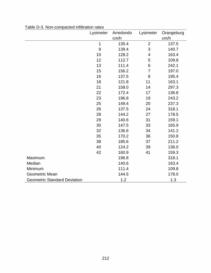
212
Table D-3. Non-compacted infiltration rates Lysimeter Arredondo Lysimeter Orangeburg
cm/h
cm/h
1 135.4 2 137.5
9 139.4 3 140.7
10 128.2 4 163.4
12 112.7 5 109.8
13 111.4 6 242.1
15 156.2 7 197.0
16 137.5 8 195.4
18 121.8 11 163.1
21 158.0 14 297.3
22 172.4 17 136.8
23 196.8 19 243.2
25 149.4 20 237.3
26 137.5 24 318.1
28 144.2 27 178.5
29 140.6 31 159.1
30 147.5 33 165.9
32 136.6 34 141.2
35 170.2 36 150.8
38 185.6 37 211.2
40 124.2 39 136.0
42 160.9 41 159.3 Maximum
196.8
318.1
Median
140.6
163.4 Minimum
111.4
109.8
Geometric Mean
144.5
178.0 Geometric Standard Deviation
1.2
1.3

213
Table D-4. Non-compacted summary of cone indices profiles. Soil Arredondo Orangeburg Depth (kPa) (kPa) (cm) Min. Median Max. Mean St. Dev. Min. Median Max. Mean St. Dev.
0.0 0 211 667 239 123 105 211 526 235 85 2.5 0 211 456 221 91 105 175 386 209 60 5.0 105 211 421 214 75 105 211 316 197 38 7.5 105 211 386 209 70 105 175 351 196 41
10.0 105 175 386 200 64 140 211 316 196 35 12.5 105 175 386 194 60 105 175 316 193 34 15.0 105 175 386 190 64 70 211 316 195 44 17.5 70 175 386 179 54 70 211 351 194 49 20.0 70 175 351 183 66 70 175 351 197 48 22.5 70 175 351 172 59 70 211 351 197 56 25.0 70 140 246 159 39 70 211 386 196 59 27.5 70 175 246 156 38 70 175 351 184 54 30.0 70 140 246 143 37 70 175 456 171 70 32.5 70 140 246 134 36 70 140 316 146 54 35.0 70 105 246 126 37 70 140 246 135 43 37.5 70 105 211 113 33 70 105 351 126 59 40.0 70 105 211 105 31 70 105 421 120 72 42.5 70 70 211 91 30 70 105 386 114 64 45.0 70 70 211 86 32 70 70 246 92 44

214
Table D-5. Student T-test results for determining whether cone index values were significantly different at each depth.
Soil Depth (cm) p-value 0.0 0.79 2.5 0.42 5.0 0.10 7.5 0.21 10.0 0.59 12.5 0.90 15.0 0.64 17.5 0.10 20.0 0.17 22.5 0.02 25.0 0.00 27.5 0.00 30.0 0.01 32.5 0.17 35.0 0.23 37.5 0.14 40.0 0.14 42.5 0.02 45.0 0.47

215
Table D-6. Compacted bulk densities. Lysimeter Arredondo Lysimeter Orangeburg
ρb (g/cm3)
ρb (g/cm3)
1 1.59 2 1.47
9 1.57 3 1.43
10 1.57 4 1.39
12 1.54 5 1.47
13 1.55 6 1.55
15 1.57 7 1.43
16 1.55 8 1.36
18 1.55 11 1.42
21 1.50 14 1.41
22 1.58 17 1.44
23 1.57 19 1.48
25 1.56 20 1.47
26 1.56 24 1.39
28 1.56 27 1.36
29 1.54 31 1.45
30 1.56 33 1.38
32 1.54 34 1.49
35 1.54 36 1.48
38 1.56 37 1.48
40 1.54 39 1.38
42 1.55 41 1.46 Maximum
1.59
1.55
Median
1.56
1.44 Minimum
1.50
1.36
Mean
1.56
1.44 Standard Deviation
0.02
0.05

216
Table D-7. Compacted infiltration rates. Lysimeter Arredondo Lysimeter Orangeburg
cm/h
cm/h
1 28.5 2 5.0
9 32.6 3 14.0
10 39.9 4 4.6
12 34.1 5 14.6
13 36.4 6 14.9
15 34.1 7 7.5
16 36.3 8 8.9
18 39.9 11 6.3
21 36.8 14 10.2
22 41.2 17 6.2
23 35.5 19 4.8
25 37.3 20 4.8
26 34.5 24 13.6
28 36.7 27 2.8
29 36.5 31 0.6
30 35.1 33 0.3
32 33.2 34 2.1
35 34.2 36 0.9
38 44.2 37 1.2
40 37.8 39 3.6
42 36.6 41 2.5 Maximum
44.2
14.9
Median
36.4
4.8 Minimum
28.5
0.3
Geometric Mean
36.1
4.1 Geometric Standard Deviation
1.1
2.9

217
Table D-8. Runoff coefficients for each Arredondo lysimeter from rainfall events during compaction phase.
#Rainfall depth accounting for flange contributions.
Effective Rainfall Depth (cm)#
Lysimeter 6.37 5.32 5.12 4.31 3.07 2.41 1.93 1.84 1 0.09 0.00 0.00 0.00 0.00 0.00 0.00 0.00 9 0.35 0.54 0.13 0.14 0.07 0.06 0.08 0.05 10 0.56 0.45 0.10 0.29 0.00 0.00 0.06 0.06 12 0.59 0.46 0.04 0.14 0.01 0.01 0.00 0.02 13 0.30 0.19 0.00 0.09 0.22 0.00 0.00 0.00 15 0.38 0.33 0.06 0.23 0.02 0.00 0.00 0.00 16 0.52 0.38 0.02 0.20 0.00 0.00 0.00 0.00 18 0.54 0.17 0.03 0.24 0.00 0.00 0.05 0.05 21 0.39 0.51 0.15 0.30 0.00 0.07 0.16 0.12 22 0.44 0.48 0.00 0.00 0.01 0.00 0.00 0.00 23 0.43 0.37 0.00 0.09 0.02 0.00 0.00 0.00 25 0.31 0.31 0.00 0.08 0.09 0.00 0.00 0.01 26 0.36 0.01 0.00 0.00 0.03 0.00 0.00 0.00 28 0.25 0.04 0.00 0.00 0.08 0.00 0.00 0.00 29 0.40 0.19 0.00 0.01 0.07 0.00 0.00 0.00 30 0.29 0.10 0.00 0.00 0.05 0.00 0.00 0.00 32 0.49 0.43 0.03 0.13 0.33 0.00 0.00 0.00 35 0.47 0.38 0.00 0.03 0.16 0.00 0.00 0.00 38 0.52 0.45 0.06 0.10 0.06 0.00 0.00 0.00 40 0.42 0.25 0.00 0.09 0.13 0.00 0.00 0.00 42 0.55 0.40 0.12 0.18 0.03 0.01 0.00 0.00

218
Table D-9. Runoff coefficients for each Orangeburg lysimeter from rainfall events during compaction phase.
#Rainfall depth accounting for flange contributions.
Effective Rainfall Depth (cm)#
Lysimeter 6.37 5.32 5.12 4.31 3.07 2.41 1.93 1.84 2 0.59 0.44 0.00 0.06 0.25 0.97 0.00 0.00 3 0.60 0.55 0.11 0.24 0.51 0.09 0.00 0.00 4 0.63 0.43 0.00 0.17 0.37 0.95 0.00 0.00 5 0.77 0.68 0.20 0.47 0.63 0.25 0.00 0.15 6 0.62 0.59 0.13 0.34 0.52 0.08 0.28 0.00 7 0.90 0.35 0.25 0.50 0.45 0.29 0.31 0.27 8 0.83 0.67 0.18 0.39 0.64 0.27 0.21 0.11 11 0.60 0.49 0.02 0.09 0.21 0.02 0.04 0.02 14 0.66 0.53 0.07 0.31 0.47 0.00 0.00 0.00 17 0.72 0.51 0.03 0.24 0.46 0.00 0.00 0.00 19 0.78 0.68 0.31 0.58 0.51 0.00 0.37 0.34 20 0.91 0.71 0.28 0.64 0.80 0.39 0.33 0.28 24 0.73 0.59 0.14 0.39 0.55 0.06 0.05 0.02 27 0.58 0.53 0.07 0.13 0.31 0.00 0.00 0.00 31 0.47 0.46 0.00 0.12 0.36 0.00 0.00 0.00 33 0.47 0.37 0.00 0.06 0.16 0.00 0.00 0.00 34 0.62 0.54 0.06 0.26 0.49 0.02 0.00 0.00 36 0.38 0.31 0.00 0.00 0.00 0.00 0.00 0.00 37 0.51 0.45 0.00 0.11 0.27 0.00 0.00 0.00 39 0.61 0.45 0.00 0.14 0.32 0.00 0.00 0.00 41 0.72 0.69 0.24 0.47 0.52 0.28 0.30 0.12

219
Table D-10. Calculated and regressed curve numbers from compacted Arredondo lysimeters.
Lysimeter Rainfall (mm) Regressed 44 37 36 30 21 17 13 13
1 70
70 9 85 92 77 81 81 85 88 87 82 10 92 90 75 87 73
87 88 87
12 92 90 69 81 74 79
84 85 13 83 80
78 89
78
15 86 87 71 85 77
95 16 90 88 67 84 73
100
18 91 79 68 86 72
87 87 80 21 86 92 79 88 72 85 91 90 87 22 88 91
76
100
23 88 88
78 77
99 25 84 86
77 83
83 82
26 85 64
78
78 28 81 69
82
70
29 87 80
68 82
93 30 83 75
65 80
86
32 90 90 69 80 92
96 35 89 88
72 86
98
38 91 90 72 78 81
93 40 87 83
78 85
86
42 91 89 77 83 78 80
92 Absent values indicate runoff was not produced from rainfall event by the corresponding lysimeter.

220
Table D-11. Calculated and regressed curve numbers from compacted Orangeburg lysimeters.
Lysimeter Rainfall (mm) Regressed 44 37 36 30 21 17 13 13
2 92 90
76 90 100
95 3 93 92 76 85 95 86
93
4 93 90
83 92 100
91 5 96 95 82 92 97 92
91 94
6 93 93 77 89 95 86 94
91 7 99 87 84 93 94 93 94 94 90 8 97 95 80 90 97 92 92 90 94 11 93 91 67 77 88 80 86 84 85 14 94 92 73 88 94
99
17 95 92 68 86 94
100 19 96 95 86 94 95
95 95 93
20 99 96 85 95 98 94 95 94 96 24 95 93 78 90 96 84 87 84 96 27 92 92 73 81 91
95
31 89 90
80 92
92 33 89 88
76 86
93
34 93 92 72 86 95 81
98 36 86 86
88
37 90 90
79 90
94 39 93 90
81 91
95
41 95 95 83 92 95 92 94 90 93 Absent values indicate runoff was not produced from rainfall event by the corresponding lysimeter.

221
Table D-12. Amendment phase Arredondo bulk densities. Lysimeter Amendment# Incorporation Depth (cm) Replicate Bulk density (g/cm3)
1 F 10 3 1.28 9 C 10 1 1.06 10 N 20 1 1.37 12 N 0 1 1.48 13 N 10 3 1.34 15 C 20 3 0.98 16 N 20 3 1.28 18 N 0 3 1.46 21 F 10 2 1.07 22 F 20 3 1.25 23 N 0 2 1.60 25 N 20 2 1.28 26 F 20 1 1.23 28 N 10 1 1.42 29 C 20 2 1.13 30 C 10 2 0.97 32 F 20 2 1.22 35 C 10 3 0.99 38 F 10 1 1.03 40 N 10 2 1.29 42 C 20 1 1.08
# Amendment – N: Null; F: Fly Ash; C: Compost

222
Table D-13. Amendment phase Orangeburg bulk densities. Lysimeter Amendment# Incorporation Depth (cm) Replicate Bulk density (g/cm3)
2 N 10 1 1.15 3 C 20 2 1.11 4 N 20 2 1.22 5 C 10 2 0.95 6 C 20 1 0.90 7 F 20 2 1.17 8 C 20 3 0.97 11 C 10 1 0.88 14 C 10 3 0.89 17 F 10 3 1.13 19 N 10 3 1.20 20 F 20 1 1.18 24 F 10 1 1.03 27 N 0 1 1.47 31 N 0 3 1.34 33 N 10 2 1.22 34 F 10 2 1.04 36 N 0 2 1.45 37 N 20 1 1.21 39 F 20 3 1.18 41 N 20 3 1.39
# Amendment – N: Null; F: Fly Ash; C: Compost

223
Table D-14. Amendment phase Arredondo infiltration rates.
Lysimeter Amendment# Incorporation Depth (cm) Replicate Infiltration Rate (cm/h)
1 F 10 3 4.0 9 C 10 1 75.4 10 N 20 1 121.9 12 N 0 1 20.0 13 N 10 3 27.9 15 C 20 3 91.7 16 N 20 3 80.5 18 N 0 3 27.8 21 F 10 2 8.2 22 F 20 3 8.6 23 N 0 2 27.1 25 N 20 2 60.4 26 F 20 1 18.6 28 N 10 1 42.2 29 C 20 2 87.8 30 C 10 2 61.3 32 F 20 2 12.6 35 C 10 3 93.7 38 F 10 1 2.5 40 N 10 2 53.0 42 C 20 1 98.8
# Amendment – N: Null; F: Fly Ash; C: Compost
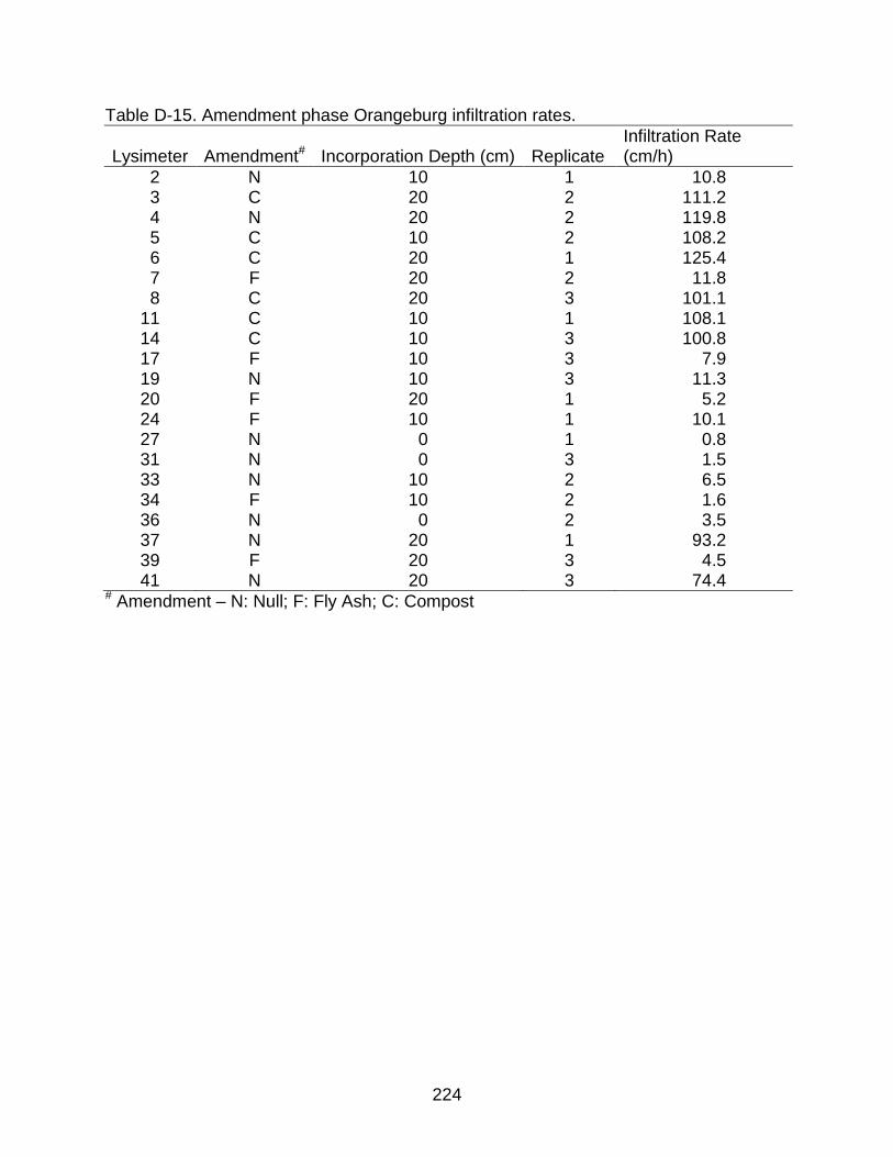
224
Table D-15. Amendment phase Orangeburg infiltration rates.
Lysimeter Amendment# Incorporation Depth (cm) Replicate Infiltration Rate (cm/h)
2 N 10 1 10.8 3 C 20 2 111.2 4 N 20 2 119.8 5 C 10 2 108.2 6 C 20 1 125.4 7 F 20 2 11.8 8 C 20 3 101.1 11 C 10 1 108.1 14 C 10 3 100.8 17 F 10 3 7.9 19 N 10 3 11.3 20 F 20 1 5.2 24 F 10 1 10.1 27 N 0 1 0.8 31 N 0 3 1.5 33 N 10 2 6.5 34 F 10 2 1.6 36 N 0 2 3.5 37 N 20 1 93.2 39 F 20 3 4.5 41 N 20 3 74.4
# Amendment – N: Null; F: Fly Ash; C: Compost

225
Table D-16. Summary of Arredondo cone index profiles indicating significant difference between control treatments. Soil depths are from control treatments referenced with maximum depth at drainage layer.
Soil Depth Treatment#
(cm) N10 N20 F10 F20 C10 C20 0.0 X* XX X XX XX XX 2.5 XX XX X XX XX XX 5.0 XX XX X XX XX XX 7.5 XX XX XX XX XX XX
10.0 XX XX XX XX XX XX 12.5 XX XX XX XX XX XX 15.0 XX XX XX XX XX XX 17.5 X XX
XX X XX
20.0
XX
XX
XX 22.5
XX
XX
XX
25.0
XX
XX
XX 27.5
XX
X
30.0
X
X 32.5
X
X
35.0
X
X 37.5 X XX
X
40.0
XX
X X 42.5
XX
X X
45.0 X XX X X *X and XX indicate significant differences at p < 0.05 and p < 0.01, respectively, from t-test analysis. #Treatment: [Amendment – N: Null; F: Fly Ash; C: Compost][Depth –10 cm, 20 cm]

226
Table D-17. Summary of Orangeburg cone index profiles indicating significant difference between control treatments. Soil depths are from control treatments referenced with maximum depth at drainage layer.
Soil Depth Treatment# (cm) N10 N20 F10 F20 C10 C20
0.0 XX* X XX X XX XX 2.5 XX X XX XX XX XX 5.0 XX XX XX XX XX XX 7.5 XX XX XX XX XX XX
10.0 XX XX XX XX XX XX 12.5 XX XX XX XX XX XX 15.0 XX X X XX XX XX 17.5 XX X XX XX XX XX 20.0 XX X XX XX XX XX 22.5
X XX XX XX
25.0
XX XX 27.5
X XX
30.0
X
XX 32.5
X
XX
35.0
X X XX 37.5 X XX
*X and XX indicate significant differences at p < 0.05 and p < 0.01, respectively, from t-test analysis. #Treatment: [Amendment – N: Null; F: Fly Ash; C: Compost][Depth –10 cm, 20 cm]

227
Table D-18. Arredondo amended runoff coefficients. Rainfall Depth (mm)
114.4 77.2 75.4 71.6 71.6 69.8 67.3 61.6 58.8 54.7
Treatment* Sim.# Sim. Sim. Sim. Sim. Sim. Sim. Sim. Nat. Sim. N01 0.13 0.28 0.25 0.38 0.17 0.40 0.06 0.34 0.01 0.24 N02 0.19 0.26 0.19 0.35 0.05 0.37 0.32 0.15 0.04 0.34 N03 0.42 0.42 0.43 0.57 0.16 0.55 0.41 0.35 0.20 0.55 N101 0.00 0.00 0.00 0.00 0.01 0.00 0.00 0.00 0.00 0.00 N102 0.00 0.00 0.00 0.00 0.03 0.01 0.00 0.00 0.00 0.00 N103 0.00 0.00 0.00 0.00 0.00 0.01 0.00 0.00 0.00 0.00 N201 0.00 0.00 0.01 0.01 0.07 0.01 0.00 0.02 0.01 0.01 N202 0.00 0.00 0.01 0.00 0.00 0.00 0.00 0.00 0.00 0.00 N203 0.00 0.00 0.00 0.00 0.01 0.00 0.00 0.00 0.00 0.00 F101 0.20 0.63 0.64 0.61 0.82 0.28 0.62 0.66 0.49 0.71 F102 0.15 0.46 0.73 0.67 0.69 0.70 0.56 0.69 0.50 0.66 F103 0.32 0.74 0.77 0.81 0.82 0.77 0.84 0.90 0.61 1.00 F201 0.04 0.33 0.50 0.63 0.62 0.68 0.55 0.44 0.42 0.65 F202 0.00 0.00 0.52 0.53 0.41 0.68 0.48 0.29 0.39 0.57 F203 0.04 0.53 0.64 0.73 0.72 0.76 0.59 0.55 0.45 0.71 C101 0.34 0.00 0.00 0.01 0.00 0.00 0.01 0.01 0.01 0.01 C102 0.00 0.00 0.00 0.01 0.00 0.00 0.00 0.00 0.00 0.05 C103 0.00 0.00 0.00 0.00 0.02 0.00 0.00 0.00 0.00 0.00 C201 0.00 0.00 0.00 0.00 0.00 0.00 0.00 0.00 0.00 0.00 C202 0.00 0.00 0.00 0.00 0.00 0.00 0.00 0.00 0.00 0.00 C203 0.00 0.00 0.00 0.00 0.00 0.00 0.00 0.00 0.00 0.00
*Treatment: [Amendment – N: Null; F: Fly Ash; C: Compost][Depth – 0 cm, 10 cm, 20 cm][Replicate] #Sim.: Simulated; Nat.: Natural.

228
Table D-18. Arredondo amended runoff coefficients. Rainfall Depths (mm)
50.4 34.8 29.5 25.3 19.2 14.5 12.3 5.4 4.4
Treatment* Sim.# Nat. Nat. Nat. Nat. Nat. Nat. Nat. Nat. N01 0.41 0.04 0.04 0.00 0.01 0.02 0.00 0.06 0.03 N02 0.38 0.00 0.14 0.01 0.16 0.13 0.01 0.02 0.00 N03 0.65 0.08 0.24 0.12 0.24 0.36 0.04 0.11 0.03 N101 0.05 0.01 0.00 0.01 0.01 0.01 0.03 0.03 0.00 N102 0.00 0.00 0.00 0.02 0.09 0.00 0.00 0.00 0.00 N103 0.01 0.02 0.04 0.01 0.02 0.04 0.00 0.08 0.00 N201 0.01 0.10 0.01 0.01 0.01 0.01 0.01 0.00 0.00 N202 0.02 0.00 0.06 0.05 0.00 0.12 0.00 0.00 0.00 N203 0.00 0.00 0.00 0.00 0.02 0.01 0.00 0.00 0.00 F101 0.80 0.12 0.34 0.44 0.45 0.54 0.00 0.00 0.16 F102 0.77 0.13 0.39 0.44 0.45 0.59 0.00 0.00 0.17 F103 0.76 0.24 0.34 0.43 0.38 0.60 0.00 0.00 0.16 F201 0.79 0.00 0.27 0.13 0.20 0.37 0.00 0.00 0.02 F202 0.68 0.00 0.23 0.16 0.14 0.38 0.00 0.00 0.09 F203 0.93 0.12 0.29 0.34 0.39 0.50 0.00 0.00 0.08 C101 0.00 0.01 0.01 0.00 0.01 0.01 0.03 0.00 0.00 C102 0.00 0.00 0.00 0.00 0.00 0.00 0.00 0.00 0.00 C103 0.00 0.00 0.00 0.00 0.00 0.00 0.00 0.00 0.00 C201 0.00 0.00 0.00 0.00 0.00 0.00 0.00 0.00 0.00 C202 0.00 0.00 0.00 0.00 0.00 0.00 0.00 0.00 0.00 C203 0.00 0.00 0.00 0.00 0.00 0.00 0.00 0.00 0.00
*Treatment: [Amendment – N: Null; F: Fly Ash; C: Compost][Depth – 0 cm, 10 cm, 20 cm][Replicate] #Sim.: Simulated; Nat.: Natural.

229
Table D-19. Orangeburg amended runoff coefficients. Rainfall Depth (mm)
114.4 77.2 75.4 71.6 71.6 69.8 67.3 61.6 58.8 54.7
Treatment* Sim.# Sim. Sim. Sim. Sim. Sim. Sim. Sim. Nat. Sim. N01 0.43 0.39 0.42 0.61 0.52 0.65 0.43 0.57 0.55 0.54 N02 0.45 0.47 0.43 0.58 0.66 0.63 0.47 0.69 0.54 0.58 N03 0.30 0.41 0.53 0.62 0.58 0.72 0.52 0.68 0.63 0.66 N101 0.01 0.03 0.11 0.32 0.12 0.40 0.02 0.06 0.37 0.11 N102 0.00 0.00 0.09 0.21 0.16 0.68 0.03 0.03 0.51 0.10 N103 0.02 0.03 0.09 0.25 0.26 0.52 0.03 0.15 0.65 0.10 N201 0.02 0.00 0.04 0.08 0.00 0.01 0.01 0.00 0.39 0.03 N202 0.00 0.00 0.02 0.02 0.12 0.19 0.01 0.01 0.30 0.02 N203 0.00 0.00 0.02 0.04 0.22 0.33 0.01 0.00 0.26 0.03 F101 0.20 0.56 0.43 0.69 0.64 0.77 0.60 0.78 0.62 0.68 F102 0.22 0.42 0.57 0.69 0.56 0.71 0.53 0.65 0.54 0.66 F103 0.21 0.47 0.45 0.72 0.46 0.71 0.64 0.50 0.59 0.67 F201 0.17 0.51 0.60 0.83 0.41 0.86 0.74 0.73 0.62 0.72 F202 0.17 0.32 0.50 0.69 0.46 0.70 0.53 0.57 0.55 0.66 F203 0.17 0.47 0.55 0.74 0.54 0.13 0.50 0.77 0.68 0.67 C101 0.01 0.02 0.04 0.05 0.22 0.25 0.02 0.03 0.48 0.03 C102 0.00 0.00 0.00 0.01 0.06 0.06 0.00 0.00 0.29 0.00 C103 0.00 0.00 0.00 0.01 0.09 0.16 0.00 0.00 0.09 0.00 C201 0.00 0.00 0.02 0.11 0.20 0.30 0.01 0.04 0.41 0.02 C202 0.00 0.00 0.01 0.05 0.13 0.28 0.01 0.01 0.18 0.02 C203 0.01 0.02 0.15 0.18 0.26 0.38 0.01 0.03 0.25 0.02
*Treatment: [Amendment – N: Null; F: Fly Ash; C: Compost][Depth – 0 cm, 10 cm, 20 cm][Replicate] #Sim.: Simulated; Nat.: Natural.

230
Table D-19 Continued.
Rainfall Depths (mm)
50.4 34.8 29.5 25.3 19.2 14.5 12.3 5.4 4.4
Treatment* Sim.# Nat. Nat. Nat. Nat. Nat. Nat. Nat. Nat. N01 0.73 0.24 0.26 0.21 0.21 0.41 0.00 0.00 0.03 N02 0.69 0.15 0.26 0.17 0.20 0.38 0.00 0.00 0.00 N03 0.79 0.36 0.38 0.47 0.44 0.63 0.00 0.00 0.05 N101 0.13 0.02 0.13 0.06 0.21 0.39 0.01 0.00 0.02 N102 0.35 0.09 0.17 0.07 0.09 0.42 0.00 0.03 0.00 N103 0.47 0.35 0.23 0.24 0.23 0.57 0.01 0.00 0.02 N201 0.47 0.05 0.21 0.15 0.05 0.32 0.00 0.00 0.00 N202 0.10 0.00 0.16 0.05 0.15 0.22 0.00 0.00 0.02 N203 0.37 1.00 0.31 0.08 0.38 0.25 0.00 0.00 0.00 F101 0.87 0.35 0.43 0.52 0.61 0.70 0.00 0.00 0.09 F102 0.85 0.09 0.26 0.33 0.22 0.47 0.00 0.00 0.03 F103 0.79 0.30 0.36 0.52 0.47 0.59 0.00 0.00 0.12 F201 0.86 0.33 0.27 0.58 0.40 0.59 0.00 0.00 0.12 F202 0.65 0.16 0.26 0.39 0.29 0.55 0.00 0.00 0.12 F203 0.88 0.44 0.36 0.58 0.51 0.66 0.00 0.00 0.00 C101 0.42 0.14 0.16 0.08 0.25 0.31 0.13 0.08 0.06 C102 0.02 0.01 0.11 0.00 0.18 0.16 0.00 0.00 0.02 C103 0.08 0.00 0.16 0.01 0.15 0.09 0.00 0.00 0.00 C201 0.28 0.00 0.41 0.06 0.42 0.26 0.00 0.00 0.00 C202 0.28 0.00 0.27 0.06 0.25 0.25 0.00 0.00 0.00 C203 0.31 0.00 0.28 0.02 0.28 0.23 0.00 0.00 0.00
*Treatment: [Amendment – N: Null; F: Fly Ash; C: Compost][Depth – 0 cm, 10 cm, 20 cm][Replicate] #Sim.: Simulated; Nat.: Natural.

231
Table D-20. Calculated curve numbers for amended Arredondo lysimeters.
Rainfall Depth (mm)
*Treatment 114 77 75 72 72 70 62 67 59 55 N01 52 72 71 79 66 81 80 57 51 77 N02 57 71 67 78 54 79 68 77 58 81 N03 73 80 81 87 66 87 80 81 73 89 N101 a
44 47 44
N102
44 52 46
49 N103
44 44 47
N201
46 46 57 49 53 47 52 55 N202
45 44 43
50
N203
48 F101 58 89 89 89 95 74 92 90 87 94
F102 54 82 93 91 92 92 93 87 87 93 F103 67 93 94 95 95 94 98 96 91 100 F201 41 75 84 90 89 91 84 87 84 92 F202
42 85 86 81 92 77 84 83 90
F203 42 85 89 93 92 94 88 89 85 94 C101 68
44 47 43 45 50 49 52 54
C102
44 48 43 46
61 C103
49
C201 C202
43 C203
Absent values indicate runoff was not produced for the event by the corresponding lysimeter. a Curve numbers were not calculated when less than 100 ml of runoff was produced. *Treatment: [Amendment – N: Null; F: Fly Ash; C: Compost][Depth – 0 cm, 10 cm, 20 cm][Replicate]

232
Table D-20 Continued Rainfall Depth (mm) *Treatment 50 35 30 25 19 15 12 5 4 Regressed N001 85 69 74 70 76 83 a 94 95 70 N002 84
81 72 88 90 84 93
72
N003 93 74 86 82 90 95 87 96 94 82 N101 63 63 66 72 78 81 86 94
54
N102 53
66 73 84
39 N103 54 68 73 72 79 85
95
54
N201 56 76 68 72 77 81 84
45 N202 59
75 78 75 89
44
N203
65
78 82
44 F101 96 77 89 93 95 97
97 89
F102 96 78 90 93 95 97
97 90 F103 95 84 89 93 93 97
97 94
F201 96 62 87 83 89 95
94 86 F202 94
85 84 87 95
96 82
F203 99 77 88 91 94 96
96 90 C101 54 66 68 70 76 81 86
41
C102
66
74
38 C103
65
75
40
C201
66
75
48 C202
65
75
34
C203 66 74 50 Absent values indicate runoff was not produced for the event by the corresponding lysimeter. a Curve numbers were not calculated when less than 100 ml of runoff was produced. *Treatment: [Amendment – N: Null; F: Fly Ash; C: Compost][Depth – 0 cm, 10 cm, 20 cm][Replicate]

233
Table D-21. Calculated curve numbers from amended Orangeburg soils.
Rainfall Depth (mm)
*Treatment 114 77 75 72 72 70 62 67 59 55 N001 74 79 80 89 86 90 89 82 89 89 N002 75 82 81 88 91 90 93 84 88 90 N003 65 80 85 89 88 93 92 86 91 93 N101 35 49 61 76 62 81 60 52 82 67 N102 a
58 70 66 91 55 52 87 67
N103 37 49 59 72 72 86 68 53 92 67 N201 39
52 58
49
49 83 59
N202
47 50 63 68 49 48 78 57 N203
48 54 70 77
49 77 58
F101 58 86 81 92 90 94 95 89 91 93 F102 60 80 87 91 87 92 91 86 88 93 F103 58 82 82 92 83 92 87 90 90 93 F201 55 84 88 96 81 96 94 94 91 94 F202 56 75 84 92 83 92 89 86 89 93 F203 55 82 86 93 86 64 95 85 93 93 C101 35 48 51 55 70 73 56 51 86 59 C102
43 46 56 57
78
C103
46 60 66
64 C201
48 61 68 76 57 47 84 55
C202
46 55 63 75 51 47 71 55 C203 34 47 64 68 73 80 55 48 76 56
Absent values indicate runoff was not produced for the event by the corresponding lysimeter. a Curve numbers were not calculated when less than 100 ml of runoff was produced. *Treatment: [Amendment – N: Null; F: Fly Ash; C: Compost][Depth – 0 cm, 10 cm, 20 cm][Replicate]

234
Table D-21 Continued.
Rainfall Depth (mm)
*Treatment 50 35 30 25 19 15 12 5 4 Regressed N001b 95 84 87 87 89 95 a
95 86
N002 94 79 86 85 89 95
86 N003 96 88 90 93 94 98
95 90
N101 71 67 81 78 89 95 83
94 68 N102 83 75 83 79 85 95
93
71
N103 88 88 86 88 90 97 84
94 74 N201 88 71 85 84 81 94
60
N202 68
82 77 87 92
94 62 N203 84 101 88 80 93 93
69
F101 98 88 91 94 97 98
96 91 F102 97 75 87 90 90 96
94 88
F103 96 86 90 94 95 97
96 89 F201 98 87 87 95 94 97
96 91
F202 93 80 86 92 91 97
96 87 F203 98 90 90 95 96 98
86
C101 86 79 82 80 91 94 91 95 95 67 C102 58 64 79 69 89 91
94 61
C103 66
82 73 87 88
57 C201 80
91 78 94 93
64
C202 80 63 87 78 91 93
59 C203 81 62 87 74 91 92
64
Absent values indicate runoff was not produced for the event by the corresponding lysimeter. a Curve numbers were not calculated when less than 100 ml of runoff was produced. *Treatment: [Amendment – N: Null; F: Fly Ash; C: Compost][Depth – 0 cm, 10 cm, 20 cm][Replicate]

235
Table D-22. Summary of Arredondo calculated curve numbers regressed against inverse rainfall depths.
Regression Amendment* Incorporation Depth (cm) Replicate Slope Intercept r2
N 0 1 4.4 70 0.66 N 0 2 5.1 72 0.63 N 0 3 2.7 82 0.67 N 10 1 10.4 54 0.71 N 10 2 29.2 39 0.96 N 10 3 10.1 54 0.69 N 20 1 21.5 45 0.92 N 20 2 22.9 44 0.94 N 20 3 22.8 44 0.90 F 10 1 1.5 89 0.50 F 10 2 1.4 90 0.57 F 10 3 0.4 94 0.02 F 20 1 1.1 86 0.23 F 20 2 2.1 82 0.36 F 20 3 1.0 90 0.27 C 10 1 23.4 41 0.92 C 10 2 28.2 38 0.95 C 10 3 27.1 40 0.98 C 20 1 20.1 48 0.99 C 20 2 32.4 34 0.96 C 20 3 18.1 50 0.99
* N: Null; F: Fly Ash; C: Compost

236
Table D-23. Summary of Orangeburg calculated curve numbers regressed against inverse rainfall depths.
Regression Amendment* Incorporation Depth (cm) Replicate Slope Intercept r2
N 0 1 1.7 86 0.50 N 0 2 2.1 86 0.10 N 0 3 1.3 90 0.35 N 10 1 5.9 68 0.62 N 10 2 5.5 71 0.44 N 10 3 4.6 74 0.56 N 20 1 14.7 60 0.60 N 20 2 6.5 62 0.66 N 20 3 9.2 69 0.42 F 10 1 1.2 91 0.34 F 10 2 1.0 88 0.32 F 10 3 1.7 89 0.46 F 20 1 1.1 91 0.43 F 20 2 1.9 87 0.56 F 20 3 6.3 86 0.52 C 10 1 6.7 67 0.67 C 10 2 6.4 61 0.73 C 10 3 17.5 57 0.85 C 20 1 11.4 64 0.62 C 20 2 13.3 59 0.73 C 20 3 9.7 64 0.50
* N: Null; F: Fly Ash; C: Compost

237
Figure D-1. Results from standard proctor density method for Arredondo and
Orangeburg soil samples.
Figure D-2. Curve number regression for Arredondo Null incorporation at 0 cm.
1.25
1.50
1.75
2.00
0 10 20 30 40
Bul
k D
ensi
ty (g
/cm
3)
Volumetric Water Content (%)
ArredondoOrangeburg
1.77 g/cm3
y = 4.43x + 70.10
y = 5.14x + 71.73
y = 2.66x + 81.52
0
20
40
60
80
100
0.00 1.00 2.00 3.00 4.00 5.00 6.00
Cur
ve N
umbe
r
Inverse Rainfall Depth (cm-1)
AN01
AN02
AN03

238
Figure D-3.Curve number regression for Arredondo Null incorporation at 10 cm.
Figure D-4. Curve number regression for Arredondo Null incorporation at 20 cm.
y = 10.40x + 53.74
y = 29.15x + 39.33
y = 10.08x + 53.88
0
20
40
60
80
100
0.00 1.00 2.00 3.00 4.00 5.00 6.00
Cur
ve N
umbe
r
Inverse Rainfall Depth (cm-1)
AN101
AN102
AN103
y = 21.51x + 44.75
y = 22.95x + 43.68
y = 22.78x + 43.990
20
40
60
80
100
0.00 1.00 2.00 3.00 4.00 5.00 6.00
Cur
ve N
umbe
r
Inverse Rainfall Depth (cm-1)
AN201
AN202
AN203

239
Figure D-5. Curve number regression for Arredondo Fly Ash incorporation at 10 cm.
Figure D-6. Curve number regression for Arredondo Fly Ash incorporation at 20 cm.
y = 1.43x + 89.14
y = 1.33x + 89.90
y = 0.39x + 93.820
20
40
60
80
100
0.00 1.00 2.00 3.00 4.00 5.00 6.00
Cur
ve N
umbe
r
Inverse Rainfall Depth (cm-1)
AF101
AF102
AF103
y = 1.05x + 85.82
y = 2.08x + 82.23
y = 1.01x + 89.930
20
40
60
80
100
0.00 1.00 2.00 3.00 4.00 5.00 6.00
Cur
ve N
umbe
r
Inverse Rainfall Depth (cm-1)
AF201
AF202
AF203

240
Figure D-7. Curve number regression for Arredondo Compost incorporation at 10 cm.
Figure D-8. Curve number regression for Arredondo Compost incorporation at 20 cm.
y = 23.42x + 41.19
y = 28.24x + 37.77
y = 27.07x + 39.95
0
20
40
60
80
100
0.00 1.00 2.00 3.00 4.00 5.00 6.00
Cur
ve N
umbe
r
Inverse Rainfall Depth (cm-1)
AC101
AC102
AC103
y = 20.05x + 48.48
y = 32.44x + 33.69
y = 18.15x + 50.420
20
40
60
80
100
0.00 1.00 2.00 3.00 4.00 5.00 6.00
Cur
ve N
umbe
r
Inverse Rainfall Depth (cm-1)
AC201
AC202
AC203
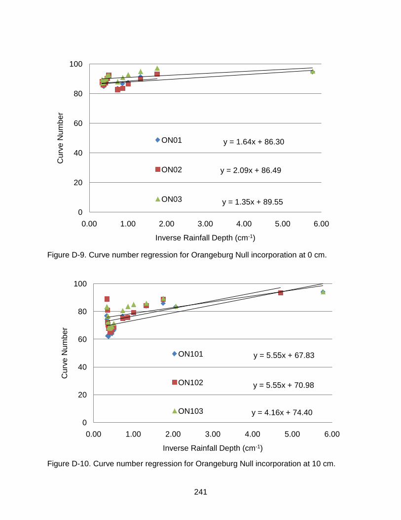
241
Figure D-9. Curve number regression for Orangeburg Null incorporation at 0 cm.
Figure D-10. Curve number regression for Orangeburg Null incorporation at 10 cm.
y = 1.64x + 86.30
y = 2.09x + 86.49
y = 1.35x + 89.550
20
40
60
80
100
0.00 1.00 2.00 3.00 4.00 5.00 6.00
Cur
ve N
umbe
r
Inverse Rainfall Depth (cm-1)
ON01
ON02
ON03
y = 5.55x + 67.83
y = 5.55x + 70.98
y = 4.16x + 74.400
20
40
60
80
100
0.00 1.00 2.00 3.00 4.00 5.00 6.00
Cur
ve N
umbe
r
Inverse Rainfall Depth (cm-1)
ON101
ON102
ON103

242
Figure D-11. Curve number regression for Orangeburg Null incorporation at 20 cm.
Figure D-12. Curve number regression for Orangeburg Fly Ash incorporation at 10 cm.
y = 14.69x + 60.47
y = 6.51x + 61.86
y = 9.20x + 69.130
20
40
60
80
100
0.00 1.00 2.00 3.00 4.00 5.00 6.00
Cur
ve N
umbe
r
Inverse Rainfall Depth (cm-1)
ON201
ON202
ON203
y = 1.18x + 91.07
y = 1.01x + 88.45
y = 1.68x + 88.90
0
20
40
60
80
100
0.00 1.00 2.00 3.00 4.00 5.00 6.00
Cur
ve N
umbe
r
Inverse Rainfall Depth (cm-1)
OF101
OF102
OF103

243
Figure D-13. Curve number regression for Orangeburg Fly Ash incorporation at 20 cm.
Figure D-14. Curve number regression for Orangeburg Compost incorporation at 10 cm.
y = 1.02x + 91.22
y = 1.85x + 87.07
y = 6.26x + 85.960
20
40
60
80
100
0.00 1.00 2.00 3.00 4.00 5.00 6.00
Cur
ve N
umbe
r
Inverse Rainfall Depth (cm-1)
OF201
OF202
OF203
y = 6.23x + 66.83
y = 6.43x + 60.89
y = 17.47x + 56.71
0
20
40
60
80
100
0.00 1.00 2.00 3.00 4.00 5.00 6.00
Cur
ve N
umbe
r
Inverse Rainfall Depth (cm-1)
OC101
OC102
OC103

244
Figure D-15. Curve number regression for Orangeburg Compost incorporation at 20 cm.
y = 11.37x + 64.39
y = 13.33x + 59.21
y = 9.74x + 63.97
0
20
40
60
80
100
0.00 1.00 2.00 3.00 4.00 5.00 6.00
Cur
ve N
umbe
r
Inverse Rainfall Depth (cm-1)
OC201
OC202
OC203

245
APPENDIX E LYSIMETER WATER QUALITY RESULTS
Table E-1. Type, date, depth and water quality results for 16 rainfall events on lysimeters.
Type Date Depth NH4-N NO2+3-N TKN OP pH
mm mg/l mg/l mg/l ug/l
Natural 10/28/09 4.4 < 0.06 < 0.15 E 0.31 27 7.26
11/25/09 58.8 E 0.14 < 0.15 E 0.18 -- 5.00
12/02/09 14.5 E 0.07 < 0.15 -- 73 5.09
12/05/09 34.8 E 0.23 < 0.15 < 0.13* -- 5.71
01/17/10 29.5 E 0.11 E 0.17 E 0.26 -- 5.30
01/22/10 19.2 E 0.11 E 0.22 E 0.24 -- 4.98
Simulated 09/23/09 114.4 E 0.14 < 0.15 E 0.39 99 7.80
09/30/09 77.2 E 0.17 E 0.18 E 0.31 107 7.08
10/07/09 61.6 E 0.07 < 0.15 E 0.19 95 7.00
10/14/09 67.3 E 0.08 < 0.15 E 0.31 111 7.23
10/21/09 54.7 E 0.12 < 0.15 E 0.24 103 7.28
11/04/09 75.4 < 0.03 < 0.15 E 0.43 107 7.08
11/12/09 50.4 E 0.10 < 0.15 E 0.32 89 7.30
11/18/09 71.6 E 0.14 < 0.15 E 0.20 53 7.32
11/23/09 69.8 E 0.11 < 0.15 0.87 89 7.56
01/13/10 71.6 E 0.09 < 0.15 E 0.24 98 7.26 E: Reported value was between practical quantitation limit and minimum detectable level. *Concentrations less than minimum detectable limit were reported are indicated as less than the respective MDL.

246
Table E-2. Concentrations from homogenous column samples. NH4-N NO2+3-N TKN Org.-N TN OP pH mg/l mg/l mg/l mg/l mg/l ug/l Arredondo E 0.15 5.47 2.31 2.16 7.78 378 6.30
E 0.17 7.57 3.48 3.31 11.05 409 6.23
E 0.16 6.46 3.35 3.18 9.81 435 6.10
E 0.16 3.64 2.57 2.41 6.21 522 5.83
Compost #-- -- -- -- -- 6642 7.51
-- -- -- -- -- 8663 7.46
-- -- -- -- -- 6613 7.40
-- -- -- -- -- 7627 7.33
Orangeburg E 0.36 14.92 0.85 E 0.49 15.77 E 9 6.64
E 0.33 19.45 E 0.31 < 0.13 19.84 15 6.70
E 0.40 17.13 E 0.40 < 0.13 17.59 E 8 6.52
E 0.33 8.12 E 0.32 < 0.13 8.51 E 8 6.15
Fly Ash E 0.27 9.18 0.82 0.54 10.00 59 7.90
-- -- -- -- -- 88 7.87
E 0.15 0.19 2.77 2.62 2.96 76 8.05
-- -- -- -- -- 81 7.84
Matrix E 0.12 < 0.15* < 0.13 < 0.13 < 0.27 E 9 8.25 E: Reported value was between practical quantitation limit and minimum detectable level. *Concentrations less than minimum detectable limit were reported are indicated as less than the respective MDL. #Values eliminated due to violations of QA/QC.

247
Table E-3. Column leachate concentrations from Arredondo and compost mixtures. Compost NH4-N NO2+3-N TKN ON TN OP pH % mg/l mg/l mg/l mg/l mg/l ug/l 5 0.71 1.68 5.63 4.91 7.30 1189 6.63
0.67 4.57 6.74 6.08 11.31 1087 6.65
#-- -- -- -- -- 1088 6.63
-- -- -- -- -- 1071 6.64
10 -- -- -- -- -- 1577 6.92
-- -- -- -- -- 1699 6.88
-- -- -- -- -- 1318 6.88
-- -- -- -- -- 1373 6.69
30 1.14 1.45 26.65 25.51 28.10 4848 7.39
-- -- -- -- -- 4553 7.36
-- -- -- -- -- 4450 7.26
-- -- -- -- -- 4908 7.29 #Values eliminated due to violations of QA/QC. Table E-4. Column leachate concentrations from Arredondo and fly ash mixtures. Fly Ash NH4-N NO2+3-N TKN ON TN OP pH % mg/l mg/l mg/l mg/l mg/l ug/l 5 E 0.12 5.20 0.61 E 0.49 5.81 204 6.36
E 0.14 3.60 1.12 0.98 4.71 191 6.25
E 0.15 7.34 0.65 0.51 7.99 196 6.43
#-- -- -- -- -- -- 6.40
10 E 0.18 4.70 2.85 2.66 7.55 181 6.09
E 0.17 4.09 0.60 E 0.43 4.69 168 6.03
E 0.14 6.30 E 0.40 E 0.26 6.70 169 6.05
E 0.19 18.51 1.07 0.87 19.57 208 5.98
30 E 0.16 4.86 0.79 0.63 5.65 160 6.59
E 0.17 1.93 0.87 0.69 2.79 171 6.66
E 0.17 1.70 0.78 0.62 2.48 160 6.88
E 0.18 6.06 0.67 E 0.49 6.73 115 6.70 E: Reported value was between practical quantitation limit and minimum detection level. #Values eliminated due to violations of QA/QC.

248
Table E-5. Column leachate concentrations from Orangeburg and compost mixtures. Compost NH4-N NO2+3-N TKN ON IN TN OP pH % mg/l mg/l mg/l mg/l mg/l mg/l ug/l 5 E 0.19 19.3 1.14 0.95 19.49 20.44 46 6.89
#-- -- -- -- -- -- 46 6.63
-- -- -- -- -- -- 29 6.61
E 0.22 15.18 0.66 E 0.44 15.4 15.84 39 6.35
10 E 0.18 2.97 1.67 1.49 3.15 4.64 50 6.63
E 0.14 6.62 0.76 0.62 6.76 7.38 56 6.61
E 0.16 17.97 0.98 0.83 18.13 18.96 47 6.59
E 0.12 17.40 0.94 0.81 17.53 18.34 47 6.68
30 E 0.16 23.45 3.57 3.41 23.61 27.02 429 7.44
E 0.19 27.34 5.19 4.99 27.54 32.53 477 7.44
-- -- -- -- -- -- 477 7.25
E 0.21 27.45 5.05 4.84 27.65 32.49 477 7.22 E: Reported value was between practical quantitation limit and minimum detectable level. #Values eliminated due to violations of QA/QC. Table E-6. Column leachate concentrations from Orangeburg and fly ash mixtures. Compost NH4-N NO2+3-N TKN ON IN TN OP pH % mg/l mg/l mg/l mg/l mg/l mg/l ug/l 5 E 0.45 17.75 0.72 E 0.27 18.20 18.47 7 6.83
E 0.46 #-- 0.70 E 0.23 -- -- 7 6.56
E 0.45 17.63 0.97 0.52 18.08 18.60 5 6.78
E 0.39 19.39 0.79 E 0.40 19.78 20.18 3 6.23
10 E 0.45 20.36 < 0.13 <0.13 20.81 20.87 21 6.70
E 0.14 18.35 -- -- 18.48 -- 14 6.38
E 0.17 13.57 0.68 0.52 13.74 14.25 12 6.04
E 0.15 10.23 0.53 E 0.38 10.39 10.76 14 6.16
30 E 0.30 10.42 0.89 0.59 10.72 11.31 22 6.93
-- -- -- -- -- -- 21 6.70
E 0.28 11.48 0.97 0.68 11.76 12.44 20 6.68
-- -- -- -- -- -- 16 6.67 E: Reported value was between practical quantitation limit and minimum detectable level. #Values eliminated due to violations of QA/QC.

249
Table E-7. Arredondo NH4-N concentrations (mg/l) Treatment 9/23/09 9/30/09 10/7/09 10/14/09 10/21/09 10/28/09 11/4/09 11/12/09 Runoff Samples
N01 E 0.21 E 0.14 E 0.14 <0.06 E 0.08 <0.06 E 0.08 E 0.09 N02 E 0.17 E 0.17 E 0.16 <0.06 E 0.07 E 0.07 <0.06 E 0.08 N03 E 0.29 E 0.21 <0.06 E 0.07 E 0.18 <0.06 E 0.20 E 0.10 N101 E 0.19 E 0.15 E 0.07 <0.06 E 0.07
<0.06 E 0.09
N102 <0.06 <0.06 <0.06
<0.06 E 0.09 N103 E 0.18 E 0.14 E 0.19 <0.06 E 0.11 <0.06 <0.06 E 0.09 N201 <0.06 <0.06 <0.06 <0.06 <0.06
N202 <0.06 E 0.10
N203 <0.06 <0.06 E 0.08
F101 E 0.18 E 0.15 <0.06 <0.06 E 0.11 <0.06 <0.06 E 0.09 F102 <0.06 <0.06 E 0.14
<0.06 E 0.20
F103 E 0.15 E 0.13 <0.06 <0.06 <0.06 <0.06 <0.06 E 0.09 F201 E 0.18 E 0.14 E 0.34 <0.06 E 0.07 <0.06 <0.06 E 0.08 F202
E 0.10 F203 E 0.20 E 0.14 E 0.16 <0.06 E 0.14
<0.06 E 0.10
C101 C102 E 0.13 E 0.08 <0.06 E 0.13
<0.06 E 0.07 C103
E 0.17
<0.06 C201 E 0.07 <0.06 E 0.09
<0.06 E 0.09
C202 E 0.15 E 0.14 E 0.07 E 0.06 E 0.12 <0.06 <0.06 E 0.09 C203 E 0.12 E 0.27 E 0.07 E 0.10 <0.06 <0.06 E 0.10 Leachate Samples
N01 E 0.14 N02 E 0.12 N03 E 0.10 E 0.08 <0.06 <0.06 <0.06
<0.06 <0.06 N101 E 0.11 E 0.09 <0.06 <0.06 <0.06
<0.06 <0.06
N102 E 0.10 E 0.10 <0.06 <0.06 <0.06
<0.06 <0.06 N103 E 0.09 N201 E 0.10 E 0.08 <0.06 <0.06 <0.06
<0.06 <0.06
N202 E 0.10 E 0.10 <0.06 <0.06 E 0.11
<0.06 <0.06 N203 E 0.11 E 0.08 <0.06 E 0.12 <0.06
<0.06 E 0.08
F101 E 0.12 E 0.10 <0.06
E 0.12 F102 E 0.11 E 0.09 E 0.19 <0.06 E 0.11
<0.06 E 0.11 F103 E 0.08
<0.06 F201 E 0.10 E 0.08
<0.06 F202 E 0.10 E 0.09 E 0.10 E 0.18 <0.06
<0.06 E 0.06 F203 E 0.12 E 0.07 E 0.15 <0.06 E 0.12
<0.06 E 0.07
C101 E 0.11 <0.06
E 0.06
<0.06 E 0.07 C102 E 0.15 E 0.10 E 0.19 <0.06 E 0.09
<0.06 E 0.07
C103 E 0.11 E 0.12 <0.06 E 0.11 E 0.12
<0.06 E 0.08 C201 E 0.13 <0.06 E 0.08 <0.06 E 0.10
<0.06 <0.06
C202 E 0.08 C203 E 0.14 Rainfall E 0.14 E 0.17 E 0.07 E 0.08 E 0.12 <0.06 <0.06 E 0.10
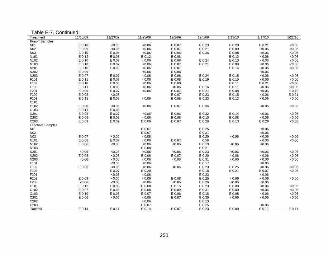
250
Table E-7. Continued. Treatment 11/18/09 11/23/09 11/25/09 12/2/09 12/5/09 1/13/10 1/17/10 1/22/10 Runoff Samples
N01 E 0.10 <0.06 <0.06 E 0.07 E 0.23 E 0.28 E 0.21 <0.06 N02 E 0.09 <0.06 <0.06 E 0.07 E 0.21 E 0.09 <0.06 <0.06 N03 E 0.10 E 0.06 <0.06 E 0.06 E 0.26 E 0.08 <0.06 <0.06 N101 E 0.12 E 0.08 E 0.12 E 0.08 E 0.12 <0.06 <0.06 N102 E 0.10 E 0.07 <0.06 E 0.08 E 0.24 E 0.13 <0.06 <0.06 N103 E 0.10 E 0.07 <0.06 E 0.07 E 0.21 E 0.09 <0.06 <0.06 N201 E 0.10 E 0.08 <0.06 E 0.07 E 0.14 <0.06 <0.06 N202 E 0.09
<0.06 E 0.08 <0.06
N203 E 0.07 E 0.07 <0.06 E 0.06 E 0.24 E 0.15 <0.06 <0.06 F101 E 0.11 E 0.07 <0.06 E 0.08 E 0.19 E 0.15 <0.06 <0.06 F102 E 0.10 E 0.08 <0.06 E 0.08 E 0.11 E 0.21 <0.06 F103 E 0.11 E 0.08 <0.06 <0.06 E 0.16 E 0.11 <0.06 <0.06 F201 E 0.09 E 0.07 <0.06 E 0.07 E 0.21 E 0.08 <0.06 E 0.19 F202 E 0.08 <0.06
E 0.07 E 0.23 E 0.15 <0.06 E 0.21
F203 E 0.11 E 0.08 <0.06 E 0.08 E 0.23 E 0.13 <0.06 <0.06 C101
C102 E 0.08 <0.06 <0.06 E 0.07 E 0.36 <0.06 <0.06 C103 E 0.11 E 0.08
C201 E 0.08 E 0.07 <0.06 E 0.06 E 0.32 E 0.14 <0.06 <0.06 C202 E 0.09 E 0.08 <0.06 E 0.06 E 0.10 E 0.08 <0.06 <0.06 C203 E 0.09 E 0.09 E 0.06 E 0.07 E 0.29 E 0.13 E 0.28 <0.06 Leachate Samples
N01
E 0.07
E 0.25 <0.06 N02
E 0.07
E 0.21 <0.06
N03 E 0.07 <0.06 <0.06
E 0.20 <0.06 <0.06 <0.06 N101 E 0.08 E 0.07 <0.06 E 0.07 0.56 <0.06 <0.06 N102 E 0.06 <0.06 <0.06 <0.06 E 0.19 <0.06 <0.06 N103
E 0.08
E 0.21
N201 <0.06 <0.06 <0.06 <0.06 E 0.23 <0.06 <0.06 <0.06 N202 E 0.08 <0.06 E 0.06 E 0.07 E 0.20 <0.06 <0.06 <0.06 N203 <0.06 <0.06 <0.06 <0.06 E 0.31 <0.06 <0.06 <0.06 F101
<0.06 <0.06
E 0.17 <0.06
F102 E 0.06 <0.06 <0.06 <0.06 E 0.23 E 0.25 <0.06 <0.06 F103
E 0.07 E 0.20
E 0.18 E 0.21 E 0.07 <0.06
F201
<0.06 <0.06
E 0.23 <0.06 F202 E 0.09 <0.06 <0.06 E 0.08 E 0.25 <0.06 <0.06 <0.06 F203 <0.06 <0.06 <0.06 <0.06 E 0.26 <0.06 <0.06 C101 E 0.12 E 0.08 E 0.08 E 0.15 E 0.23 E 0.08 <0.06 <0.06 C102 E 0.07 E 0.08 E 0.08 E 0.09 E 0.31 E 0.09 <0.06 <0.06 C103 E 0.10 E 0.08 E 0.07 E 0.08 E 0.18 E 0.08 <0.06 <0.06 C201 E 0.06 <0.06 <0.06 E 0.07 E 0.30 <0.06 <0.06 <0.06 C202
<0.06
E 0.13
C203
E 0.07
E 0.25 <0.06 Rainfall E 0.14 E 0.11 E 0.14 E 0.07 E 0.23 E 0.09 E 0.11 E 0.11

251
Table E-8. Orangeburg NH4-N concentrations (mg/l). Treatment 9/23/09 9/30/09 10/7/09 10/14/09 10/21/09 10/28/09 11/4/09 11/12/09 Runoff Samples
N01 E 0.34 E 0.13 E 0.07 E 0.08 E 0.09 <0.06 <0.06 E 0.10 N02 E 0.12 E 0.14 E 0.12
<0.06 E 0.09
N03 E 0.08
N101 E 0.15 E 0.14 E 0.14 E 0.10 E 0.14 <0.06 <0.06 E 0.09 N102
E 0.10 N103 N201 N202 E 0.12 E 0.13 E 0.28 E 0.10 E 0.15
<0.06 E 0.09
N203 F101 E 0.14 E 0.10 E 0.13
<0.06 E 0.09 F102 E 0.16 E 0.14 E 0.13
<0.06 <0.06 <0.06 E 0.08
F103 E 0.17 E 0.20 E 0.20 E 0.22 E 0.13 <0.06 <0.06 E 0.09 F201 E 0.12 E 0.13 E 0.13 E 0.08 E 0.13 <0.06 <0.06 E 0.09 F202 E 0.12 E 0.13 E 0.12 E 0.08 E 0.14
E 0.06 E 0.09
F203 E 0.12 E 0.14 E 0.14 E 0.08 E 0.12 <0.06 <0.06 E 0.09 C101
E 0.07 C102 E 0.17 E 0.15 E 0.12 <0.06 E 0.06 <0.06 <0.06 E 0.09 C103 E 0.09 E 0.19
<0.06 E 0.10
C201 E 0.20 E 0.14 E 0.30 <0.06 E 0.06 E 0.08 E 0.09 E 0.10 C202 C203 E 0.34 E 0.13 E 0.07 E 0.08 E 0.09 <0.06 <0.06 E 0.10 Leachate Samples
N01 E 0.11 E 0.08 <0.06 <0.06 E 0.09
<0.06 <0.06 N02 E 0.10 E 0.12 <0.06
N03 E 0.10 E 0.36 E 0.40 <0.06 <0.06
<0.06 <0.06 N101 E 0.10 E 0.11 <0.06 E 0.12 E 0.12
<0.06 <0.06
N102 E 0.11 <0.06 E 0.13 <0.06 <0.06
<0.06 <0.06 N103 E 0.09 N201 E 0.10 <0.06 E 0.12 <0.06 <0.06
<0.06 <0.06
N202 E 0.10 E 0.12 <0.06 E 0.10 E 0.14
<0.06 E 0.07 N203 E 0.11 <0.06 E 0.13 <0.06 <0.06
<0.06 E 0.07
F101 F102 E 0.12 E 0.10 E 0.13 E 0.24 <0.06
<0.06 F103 E 0.08 E 0.14 E 0.13 E 0.12 E 0.11
<0.06 <0.06
F201 E 0.09 <0.06 F202 E 0.10 F203 E 0.12 E 0.11 E 0.14 <0.06 E 0.12
<0.06
C101 E 0.08 C102 E 0.10 E 0.08 E 0.14 E 0.09 <0.06
<0.06 C103 E 0.09 E 0.14 E 0.09 E 0.08 E 0.13
<0.06 <0.06
C201 E 0.10 E 0.08 C202 E 0.09 E 0.11 E 0.08 E 0.07 E 0.17
<0.06 E 0.07 C203 E 0.11

252
Table E-8. Continued. Treatment 11/18/09 11/23/09 11/25/09 12/2/09 12/5/09 1/13/10 1/17/10 1/22/10 Runoff Samples
N01 E 0.12 E 0.09 <0.06 E 0.06 E 0.25 E 0.10 <0.06 <0.06 N02 E 0.11 E 0.10 <0.06 E 0.07 E 0.14 E 0.10 <0.06 <0.06 N03 E 0.10 E 0.07
E 0.08 E 0.22 E 0.17 <0.06 <0.06
N101 E 0.10 E 0.08 <0.06 <0.06 E 0.11 E 0.08 E 0.30 <0.06 N102 E 0.13 E 0.09 <0.06 E 0.07 E 0.12 E 0.13 <0.06 N103
N201
<0.06 N202 E 0.11 E 0.08 E 0.08 E 0.16 E 0.11 E 0.07 <0.06 <0.06 N203
E 0.08 E 0.14 <0.06
F101 E 0.11 E 0.06 <0.06 E 0.07 E 0.18 <0.06 <0.06 F102 E 0.10 E 0.07 <0.06 E 0.07 E 0.21 E 0.08 <0.06 <0.06 F103 E 0.10 E 0.07 E 0.06 E 0.07 E 0.18 E 0.09 <0.06 <0.06 F201 E 0.11 E 0.08 <0.06 E 0.07 E 0.23 E 0.09 <0.06 <0.06 F202 E 0.12 E 0.07 <0.06 E 0.07 E 0.16 E 0.08 <0.06 <0.06 F203 E 0.10 E 0.07 <0.06 E 0.06 E 0.23 E 0.07 <0.06 <0.06 C101
E 0.07 <0.06
E 0.12 E 0.32 <0.06
C102 E 0.12 E 0.07 <0.06 E 0.07 E 0.21 E 0.07 <0.06 E 0.16 C103 E 0.11 E 0.15 E 0.08 E 0.07 E 0.10 E 0.20 <0.06 <0.06 C201 E 0.08 <0.06 <0.06 E 0.07 E 0.24 E 0.12 <0.06 <0.06 C202
C203 E 0.12 E 0.09 <0.06 E 0.06 E 0.25 E 0.10 <0.06 <0.06 Leachate Samples
N01 <0.06 <0.06 <0.06 <0.06 E 0.28 <0.06 <0.06 <0.06 N02
<0.06 E 0.07
E 0.14 <0.06 <0.06
N03 E 0.08 <0.06 <0.06 E 0.07 E 0.28 E 0.23 <0.06 N101 E 0.07 <0.06 <0.06
E 0.11 <0.06 <0.06 <0.06
N102 E 0.08 <0.06 <0.06 E 0.06 E 0.20 <0.06 <0.06 E 0.16 N103
<0.06
E 0.12 <0.06 <0.06
N201 E 0.07 <0.06 <0.06 <0.06 E 0.23 <0.06 <0.06 <0.06 N202 E 0.10 E 0.09 E 0.07 E 0.09 E 0.24 E 0.28 <0.06 <0.06 N203 E 0.09 E 0.08 E 0.09 E 0.08 E 0.26 <0.06 <0.06 <0.06 F101
<0.06 <0.06
E 0.20 <0.06 <0.06
F102 E 0.09 <0.06 <0.06 E 0.06 E 0.22 E 0.07 E 0.23 F103 E 0.09 E 0.07 E 0.07
E 0.20 <0.06 <0.06 <0.06
F201
<0.06
E 0.20 <0.06 F202
<0.06
E 0.17
F203
<0.06 E 0.07 E 0.15 E 0.18 E 0.21 <0.06 <0.06 C101
E 0.06 <0.06
E 0.10 <0.06 <0.06
C102 E 0.07 <0.06 <0.06
E 0.22 <0.06 <0.06 C103 E 0.08 E 0.07 <0.06 E 0.07 E 0.09 E 0.07 <0.06 <0.06 C201
<0.06
E 0.24 <0.06
C202 E 0.09 E 0.07 <0.06 E 0.07 E 0.10 E 0.28 <0.06 <0.06 C203
<0.06
E 0.23

253
Table E-9. Arredondo NO2+3-N concentrations (mg/l) Treatment 9/23/09 9/30/09 10/7/09 10/14/09 10/21/09 10/28/09 11/4/09 11/12/09 Runoff Samples
N01 <0.15 <0.15 <0.15 <0.15 <0.15 <0.15 <0.15 <0.15 N02 E 0.15 <0.15 <0.15 <0.15 <0.15
<0.15 <0.15
N03 <0.15 <0.15 E 0.18 <0.15 <0.15 <0.15 <0.15 <0.15 N101
<0.15 N102
<0.15 N103
<0.15 N201 <0.15 <0.15 <0.15
<0.15 <0.15
N202 <0.15 <0.15
N203 F101 <0.15 E 0.46 <0.15 E 0.35 E 0.38 E 0.31 E 0.45 <0.15 F102 <0.15 E 0.26 <0.15 <0.15 <0.15 <0.15 E 0.27 <0.15 F103 <0.15 E 0.16 <0.15 <0.15 <0.15 <0.15 <0.15 <0.15 F201 <0.15 E 0.17 <0.15 <0.15 <0.15 <0.15 <0.15 <0.15 F202 <0.15 <0.15 <0.15 <0.15 <0.15 <0.15 <0.15 F203 <0.15 E 0.15 <0.15 <0.15 <0.15 <0.15 E 0.15 <0.15 C101 <0.15 <0.15 <0.15 <0.15
<0.15 <0.15
C102 1.09
E 0.48
C103 C201 C202 C203 Leachate Samples N01 13.76 14.62 15.39 15.24 17.60
13.81 15.42
N02 15.90 19.39 J 22.32 17.63 18.42
13.28 16.63 N03 22.40 22.30 25.80 24.98 26.29
27.54
N101 32.03 24.71 17.74 14.14 14.46
13.04 14.97 N102 25.11 26.69 18.60 13.55 12.22
10.26 14.32
N103 23.52 23.06 15.49 13.81 14.00
11.44 12.98 N201 20.62 23.32 15.99 13.20 12.74
13.65 13.74
N202 38.72 27.48 17.90 13.54 14.16
12.41 14.41 N203 30.38 29.63 18.35 14.03 15.45
13.75
F101 24.72 F102 28.59 F103 10.05 F201 28.57 23.18 20.98
17.88 F202 31.73 32.95 27.71
F203 25.61 C101 15.42 13.84 J 11.07 9.38 9.60
8.32 12.92 C102 35.94 23.46 19.93 14.51 14.35
12.97 14.65
C103 28.41 32.93 27.37 20.77 21.88
19.76 24.48 C201 33.39 25.58 17.52 12.34 13.41
11.91 15.01
C202 31.35 19.65
18.05
16.13 20.24 C203 29.71 21.29 15.31 11.33 13.25
11.30 17.73
Rainfall <0.15 E 0.18 <0.15 <0.15 <0.15 <0.15 <0.15 <0.15

254
Table E-9. Continued. Treatment 11/18/09 11/23/09 11/25/09 12/2/09 12/5/09 1/13/10 1/17/10 1/22/10 Runoff Samples
N01 <0.15 <0.15 <0.15 <0.15 <0.15 <0.15 <0.15 <0.15 N02 <0.15 <0.15 E 0.18 <0.15 <0.15 E 0.16 <0.15 N03 <0.15 0.04 <0.15 <0.15 <0.15 <0.15 <0.15 <0.15 N101 <0.15 <0.15
<0.15 <0.15 E 0.26 <0.15 <0.15
N102
<0.15 <0.15
E 0.24 <0.15 <0.15 N103 <0.15 <0.15
<0.15 <0.15 E 0.27 <0.15 <0.15
N201 <0.15 <0.15 <0.15 <0.15 <0.15 <0.15 <0.15 <0.15 N202 <0.15
<0.15 <0.15 <0.15
N203
<0.15 E 0.16 <0.15 F101 <0.15 <0.15 <0.15 <0.15 <0.15 Y E 0.21 <0.15 <0.15 F102 <0.15 <0.15 <0.15 <0.15 <0.15 <0.15 <0.15 <0.15 F103 <0.15 <0.15 E 0.21 <0.15 <0.15 E 0.36 <0.15 <0.15 F201 <0.15 <0.15 <0.15 <0.15 <0.15 E 0.19 <0.15 <0.15 F202 <0.15 <0.15 <0.15 <0.15 E 0.16 <0.15 <0.15 F203 <0.15 <0.15 E 0.18 <0.15 E 0.21 E 0.16 <0.15 <0.15 C101 <0.15 <0.15 <0.15 <0.15 <0.15 <0.15 <0.15 C102 E 0.32 E 0.29
C103
C201
C202
C203
<0.15
Leachate Samples
N01 15.17 14.85 8.30 4.76 4.03 1.48 5.03 N02 16.78 15.05 11.20 4.44 3.73 6.58 6.82 N03
25.64 20.36 12.89 10.58 6.93 7.00 7.33
N101 12.94 8.02 4.29 2.71 2.57 4.23 7.68 7.52 N102 11.76 8.91 6.60 2.61 2.65 Y 2.80 7.99 8.57 N103 12.27 9.61 5.63 3.54 2.90 3.83 7.18 7.31 N201 12.77 8.63 3.67 3.13 2.78 4.33 5.19 5.69 N202 10.62 5.88 5.21 3.38 3.19 5.62 7.68 7.73 N203 13.43 8.47 4.23 2.52 2.60 3.99 4.74 F101
54.88 J
67.66 Y
F102
46.26 J
61.92 F103
11.85 J
35.60 17.87
F201
20.40 29.69
39.53 20.76 F202
8.26 20.58
38.85 26.14 23.21
F203
44.49 J
48.36 46.47 C101 12.54 9.89 6.28 3.62 3.55 3.61 9.72 11.83 C102 13.58 9.95 5.97 4.84 4.61 6.80 13.23 13.15 C103 22.61 17.63 11.16 6.88 6.74 6.17 12.84 14.02 J C201 13.67 11.00 2.83 4.68 3.88 6.30 13.63 13.88 C202 20.31 14.62 7.53 6.11 5.30 6.36 13.54 13.91 C203 15.80 13.26 8.27 5.15 5.30 6.79 13.35 14.41 Rainfall <0.15 <0.15 <0.15 <0.15 <0.15 <0.15 E 0.17 E 0.22

255
Table E-10. Orangeburg NO2+3-N concentrations (mg/l) Treatment 9/23/09 9/30/09 10/7/09 10/14/09 10/21/09 10/28/09 11/4/09 11/12/09 Runoff Samples
N01 E 0.15 E 0.18 <0.15 E 0.2 <0.15 <0.15 <0.15 <0.15 N02 <0.15 E 0.24 <0.15 E 0.37 E 0.29
<0.15 <0.15
N03 <0.15 <0.15 <0.15 E 0.3 E 0.20 <0.15 <0.15 <0.15 N101 <0.15 <0.15 <0.15 <0.15 <0.15 <0.15 <0.15 <0.15 N102 E 0.18 <0.15 <0.15
<0.15 <0.15
N103 <0.15 E 0.17 E 0.15 <0.15 E 0.16 0.66 <0.15 <0.15 N201 <0.15 <0.15 <0.15
<0.15 <0.15
N202 <0.15 <0.15 <0.15 <0.15 <0.15 N203 <0.15 <0.15
<0.15 <0.15
F101 <0.15 E 0.19 E 0.22 E 0.17 E 0.25 <0.15 <0.15 <0.15 F102 <0.15 E 0.15 <0.15 <0.15 E 0.15 <0.15 Y <0.15 <0.15 F103 <0.15 E 0.25 <0.15
<0.15 <0.15 <0.15 <0.15
F201 <0.15 E 0.23 <0.15 <0.15 E 0.17 <0.15 <0.15 <0.15 F202 <0.15 <0.15 <0.15 <0.15 <0.15 <0.15 <0.15 <0.15 F203 <0.15 <0.15 <0.15 <0.15 0.05
<0.15 <0.15
C101 E 0.18 <0.15 <0.15 <0.15 <0.15 <0.15 <0.15 C102
<0.15 <0.15 <0.15 C103
<0.15 C201 <0.15 0.56 E 0.17
<0.15 <0.15
C202 E 0.21 0.50 <0.15
<0.15 <0.15 C203 <0.15 E 0.2 E 0.18 0.61 <0.15
<0.15 <0.15
Leachate Samples N01 12.11
13.51 N02 N03 7.22 N101 3.60 4.44 4.74 4.49 5.43
3.91 5.10 N102 8.46 7.17 7.09 6.37 6.65
6.42 6.94
N103 9.24 11.51 11.63 10.31 10.02
8.25 N201 5.83 5.85 5.06 5.79 6.91
4.98 7.15
N202 6.95 5.93 6.45 6.21 6.92
5.30 6.78 N203 13.44 9.37 10.46 8.01 8.05
6.79 7.66
F101 7.84 F102 4.15 F103 7.16 <0.15 F201 9.28 11.22 F202 7.16 J 7.82
8.14 F203 8.22 C101 5.08 4.57 4.36 5.58 6.72
5.76 8.19 C102 6.89 7.18 7.74 6.51 6.62
4.43 5.65
C103 7.48 6.72 7.56 7.85 8.13
6.87 8.42 C201 5.70 5.44 5.97 5.10 5.89
6.17 7.87
C202 15.25 12.25 14.19 10.63 10.01
10.14 12.67 C203 9.50 7.63 8.21 7.43 8.96
8.01 10.28

256
Table E-10. Continued. Treatment 11/18/09 11/23/09 11/25/09 12/2/09 12/5/09 1/13/10 1/17/10 1/22/10 Runoff Samples
N01 <0.15 <0.15 <0.15 <0.15 <0.15 <0.15 <0.15 <0.15 N02 <0.15 <0.15 <0.15 <0.15 <0.15 <0.15 <0.15 <0.15 N03 <0.15 <0.15 <0.15 <0.15 <0.15 Y <0.15 <0.15 <0.15 N101 <0.15 <0.15 <0.15 <0.15 E 0.24 <0.15 <0.15 <0.15 N102 <0.15 <0.15 <0.15 <0.15 E 0.15 <0.15 <0.15 <0.15 N103 <0.15 <0.15 <0.15 <0.15 <0.15 <0.15 <0.15 <0.15 N201 <0.15 <0.15 <0.15 <0.15 <0.15 Y <0.15 <0.15 N202 <0.15 <0.15 <0.15 <0.15 E 0.21 <0.15 <0.15 N203 <0.15 <0.15 <0.15 <0.15 <0.15 Y <0.15 <0.15 <0.15 F101 <0.15 <0.15 <0.15 <0.15 <0.15 E 0.25 <0.15 <0.15 F102 <0.15 <0.15 <0.15 <0.15 <0.15 <0.15 <0.15 <0.15 F103 <0.15 <0.15 <0.15 <0.15 <0.15 <0.15 <0.15 <0.15 F201 <0.15 <0.15 <0.15 <0.15 <0.15 <0.15 <0.15 <0.15 F202 <0.15 <0.15 <0.15 <0.15 <0.15 E 0.17 <0.15 <0.15 F203 <0.15 <0.15 E 0.15 <0.15 E 0.26 Y <0.15 <0.15 <0.15 C101 <0.15 <0.15 <0.15 <0.15 <0.15 <0.15 <0.15 <0.15 C102 E 0.17 <0.15 <0.15 <0.15 <0.15 E 0.23 <0.15 <0.15 C103 E 0.34 <0.15 <0.15 <0.15 <0.15 <0.15 <0.15 C201 <0.15 <0.15 <0.15 <0.15 E 0.17 <0.15 <0.15 C202 <0.15 <0.15 <0.15 <0.15 <0.15 E 0.30 <0.15 <0.15 C203 <0.15 <0.15 <0.15 <0.15 <0.15 <0.15 <0.15 <0.15 Leachate Samples
N01
14.63 12.86
11.35 8.90 7.31 7.02 N02
2.22 2.54
8.63 5.76 5.04
N03
4.66
11.53 N101 5.66 6.17 5.83
5.39 3.17 3.66 3.83
N102 6.80 6.93 6.05
6.02 4.99 4.07 3.96 N103 9.22 8.79 2.95
7.91 5.11 4.63
N201 6.79 6.31 5.98
4.57 Y 2.74 2.99 3.30 N202 6.37 5.73 4.71 4.61 4.88 3.04 2.92 2.76 N203 7.11 5.80 4.65 4.36 4.33 Y 3.14 3.27 2.86 F101
2.48
14.02
F102
5.47
10.08 10.83 10.16 F103
6.37
10.83 12.64
F201
9.18
14.88 12.91 F202
7.40 10.58
11.61 10.17
F203
11.87 12.50
14.73 Y 14.13 12.12 C101 6.46 7.93 8.35 8.64 8.28 4.47 7.56 7.00 C102 5.88 5.51 4.05 3.22 3.10 2.22 4.28 4.12 C103 8.78 7.39 6.13 5.49 4.91 3.93 5.52 4.94 C201 8.27 9.12 9.81 7.24 8.18 6.21 7.88 7.45 C202 12.57 11.47 9.01 7.55 7.85 6.01 11.09 C203 10.33 10.15 8.81 7.88 7.58 5.04 7.74
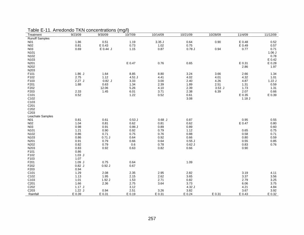
257
Table E-11. Arredondo TKN concentrations (mg/l) Treatment 9/23/09 9/30/09 10/7/09 10/14/09 10/21/09 10/28/09 11/4/09 11/12/09 Runoff Samples
N01 1.86 0.51 1.19 3.35 J 0.64 0.90 E 0.48 0.52 N02 0.81 E 0.43 0.73 1.02 0.75 E 0.49 0.57 N03 0.69 E 0.44 J 1.15 0.87 0.78 J 0.94 0.77 0.71 N101 1.06 J N102 0.78 N103 E 0.42 N201 E 0.47 0.76 0.65 E 0.31 E 0.28 N202 2.86 1.97 N203 F101 1.86 J 1.64 8.85 8.80 3.24 3.66 2.66 1.34 F102 2.75 1.12 4.51 J 4.41 4.02 4.01 4.32 1.01 F103 2.27 J 0.82 J 3.33 3.00 2.40 4.26 4.87 1.22 J F201 1.88 0.63 1.34 2.39 1.89 2.51 1.31 0.59 F202 12.06 5.26 4.10 2.39 3.53 J 1.73 1.31 F203 2.33 1.45 6.01 3.71 2.38 6.39 2.07 0.66 C101 0.52 1.22 0.52 0.61 E 0.35 E 0.39 C102 3.08 1.18 J C103 C201 C202 C203 Leachate Samples
N01 0.81 0.61 0.53 J 0.68 J 0.87 0.95 0.55 N02 1.04 0.81 0.62 0.81 0.62 E 0.47 0.80 N03 0.98 0.91 0.86 J 0.89 0.89 0.60 N101 1.21 0.90 0.92 0.79 1.12 0.65 0.75 N102 0.86 0.71 0.75 0.76 0.88 0.58 0.71 N103 0.86 0.71 J 0.64 0.92 0.66 0.80 0.59 N201 0.91 0.79 0.66 0.64 0.55 J 0.55 0.85 N202 0.82 0.79 0.6 0.78 0.62 J 0.83 0.76 N203 0.83 0.92 0.63 0.82 0.66 0.90 F101 0.86 F102 1.03 J F103 1.07 F201 1.09 J 0.75 0.64 1.09 F202 0.82 J 0.92 J 0.67 F203 0.94 C101 1.29 2.08 2.35 2.95 2.82 3.19 4.11 C102 1.13 1.95 2.15 2.62 3.65 3.37 3.56 C103 1.01 1.92 J 1.53 2.71 0.82 2.79 3.25 C201 1.66 2.36 2.75 3.64 3.73 6.06 3.75 C202 1.17 J 3.12 4.32 J 4.21 4.84 C203 1.22 J 0.94 2.51 3.26 3.82 3.67 3.92 Rainfall E 0.39 E 0.31 E 0.19 E 0.31 E 0.24 E 0.31 E 0.43 E 0.32

258
Table E-11. Continued. Treatment 11/18/09 11/23/09 11/25/09 12/2/09 12/5/09 1/13/10 1/17/10 1/22/10 Runoff Samples
N01 E 0.23 0.59 0.51 0.72 <0.13 Q 1.95 1.66 J 1.74 N02 E 0.42 E 0.41 2.86 7.54 1.98 11.25 15.04 N03 E 0.31 0.62 J E 0.45 3.68 E 0.26 Q 3.85 6.58 9.46 N101 1.77 1.40 0.96 J E 0.43 Q 1.52 0.58 0.62 N102 1.21 J 2.75 2.47 0.59 11.74 N103 0.59 J 1.02 1.58 <0.13 Q 1.04 0.56 1.45 N201 E 0.35 0.87 <0.13 0.55 E 0.14 Q 4.01 E 0.48 0.77 N202 1.03 3.02 1.79 6.21 N203 4.78 1.26 6.8 F101 1.38 1.82 0.96 1.78 1.43 Q,Y,J 1.7 6.14 9.11 F102 1.30 0.88 E 0.41 1.38 0.63 Q 2.08 3.19 7.23 F103 1.2 J 0.74 J 1.40 J 1.84 <0.13 Q 1.06 2.44 5.64 F201 0.59 J E 0.43 <0.13 5.15 E 0.32 Q 1.59 7.16 6.15 F202 1.09 0.85 E 0.34 4.01 1.27 5.43 7.58 F203 0.84 0.66 E 0.26 1.52 0.54 Q 1.03 4.47 3.01 C101 E 0.26 0.83 E 0.14 0.55 E 0.22 Q E 0.4 0.64 C102 3.43 1.69 C103 C201 C202 C203 1.2 Leachate Samples
N01 0.65 1.02 0.63 0.8 0.71 Q 0.75 J 0.84 N02 0.73 1.33 0.66 0.81 1.17 Q 0.86 1.05 J N03 1.15 0.69 1.1 J 0.97 Q 1.1 1.02 1.28 N101 0.66 1.5 0.64 0.99 0.6 Q 0.66 0.74 J 0.8 N102 0.7 0.95 0.8 0.72 0.64 Q,Y 0.75 0.71 0.86 N103 0.72 1.05 0.56 0.88 0.61 Q 0.69 0.74 1.17 J N201 0.74 1.33 E 0.49 0.76 0.78 Q 0.72 0.81 0.92 N202 0.72 0.9 0.63 0.66 0.78 Q 0.72 0.85 1.01 J N203 0.92 1.12 0.68 0.83 0.66 Q 0.85 0.73 F101 E 0.5 E 0.47 Q,Y F102 0.88 0.77 Q F103 0.61 Q 0.64 F201 1.21 E 0.48 0.59 Q 0.71 F202 <0.13 J E 0.48 E 0.47 Q 0.52 0.74 F203 0.66 0.82 Q 0.55 C101 3.73 5.25 5.44 4.23 4.23 Q 3.53 3.66 4.33 C102 4.32 4.92 4.34 3.53 3.11 Q 3.43 3.04 3.74 C103 2.93 3.82 3.57 3.44 3.56 Q 3.41 1.54 3.49 C201 4.27 5.11 2.4 3.32 3.18 Q 3.86 3.31 2.02 C202 3.96 5.69 4.62 4.09 3.75 Q 3.85 2.55 3.28 C203 4.26 6.68 6.77 4.77 5.51 Q 4.2 3.97 4.39 Rainfall E 0.2 0.87 E 0.18 E 0.36 J <0.13 Q E 0.24 E 0.26 E 0.24

259
Table E-12. Orangeburg TKN concentrations (mg/l) Treatment 9/23/09 9/30/09 10/7/09 10/14/09 10/21/09 10/28/09 11/4/09 11/12/09 Runoff Samples
N01 E 0.42 E 0.4 0.81 0.95 0.65 1.6 0.76 E 0.42 N02 <0.13 0.52 0.6 0.79 <0.13 0.58 J E 0.42 N03 0.6 E 0.46 1.03 1.06 1.39 1.77 1.15 0.66 N101 0.87 0.96 J E 0.24 0.58 1.22 1.25 2.16 0.69 N102 0.59 E 0.16 1 0.53 E 0.4 N103 E 0.48 0.6 0.79 1.26 1.28 1.25 2.25 E 0.25 N201 E 0.27 1.1 0.73 J 0.69 E 0.47 N202 0.7 1.59 0.75 1.12 0.73 N203 1.35 1.1 1.31 E 0.37 F101 1.36 E 0.41 2.27 1.22 0.92 1.18 1.15 0.5 F102 1.2 E 0.47 0.9 1.16 E 0.16 J 1.1 Y <0.13 E 0.47 F103 0.85 E 0.47 1.48 1.16 0.87 0.71 E 0.31 F201 0.52 0.55 1.17 1.5 0.84 1.13 0.78 E 0.44 F202 0.75 E 0.4 J 0.85 J 1.09 0.77 0.74 J 1 E 0.34 F203 1.4 E 0.48 0.9 1.22 1.37 1.19 0.61 C101 E 0.41 E 0.31 E 0.34 E 0.48 0.55 0.75 0.5 C102 1.18 0.83 1.02 C103 E 0.42 C201 1.32 0.78 1.95 0.9 6.6 C202 0.59 J 1.02 2.29 0.73 0.59 C203 0.99 0.78 1.1 1.23 0.87 0.83 J E 0.43 Leachate Samples
N01 0.51 0.53 N02 N03 E 0.14 N101 E 0.25 E 0.16 J <0.13 E 0.21 <0.13 E 0.18 <0.13 N102 E 0.28 E 0.17 E 0.14 E 0.19 E 0.2 <0.13 0.57 N103 E 0.26 E 0.14 E 0.15 E 0.18 E 0.13 <0.13 N201 E 0.45 E 0.27 <0.13 E 0.22 E 0.15 <0.13 J E 0.34 N202 E 0.33 E 0.27 J <0.13 E 0.17 <0.13 E 0.18 <0.13 N203 0.63 E 0.35 E 0.49 E 0.31 E 0.16 E 0.28 E 0.41 F101 E 0.17 F102 E 0.22 F103 E 0.23 1.15 F201 E 0.31 <0.13 F202 E 0.2 E 0.19 J E 0.16 F203 E 0.46 C101 0.99 0.93 1.43 1.21 0.83 J 0.5 E 0.36 C102 0.69 0.73 J E 0.27 E 0.36 <0.13 E 0.38 0.8 C103 0.78 0.56 E 0.35 0.52 E 0.33 E 0.39 E 0.26 C201 0.87 0.61 J 0.51 0.7 E 0.48 0.54 J 7.56 C202 0.78 0.75 J <0.13 E 0.44 E 0.3 0.65 0.75 C203 1.07 0.78 0.65 0.65 J 0.57 0.53 1.28

260
Table E-12.Continued. Treatment 11/18/09 11/23/09 11/25/09 12/2/09 12/5/09 1/13/10 1/17/10 1/22/10 Runoff Samples
N01 E 0.43 E 0.33 <0.13 2.34 E 0.23 Q E 0.47 0.81 1.85 N02 E 0.29 E 0.44 E 0.28 0.76 E 0.29 Q 0.51 2.95 2.67 N03 0.58 0.66 E 0.38 1.33 <0.13 Q,Y E 0.28 0.66 7.53 N101 E 0.5 0.76 <0.13 0.86 E 0.35 Q 0.52 2 0.93 N102 E 0.31 0.7 J <0.13 1.92 0.58 Q 0.71 3.45 1.79 N103 0.75 J 0.72 0.73 1.58 0.6 Q 0.77 2.33 4.63 N201 0.91 0.98 E 0.32 1.38 E 0.36 Q,Y 4.69 0.92 N202 0.9 0.83 E 0.41 1.67 0.57 1.07 E 0.43 N203 2.25 0.52 0.62 2.15 E 0.46 Q,Y 1.45 0.82 7.96 F101 0.53 0.68 E 0.25 0.56 0.58 Q E 0.41 J 1.52 2.53 F102 0.54 0.8 J E 0.35 1.84 E 0.36 Q E 0.48 1.77 3.18 F103 0.52 0.54 E 0.22 2.15 E 0.27 Q <0.13 1.13 2.33 F201 E 0.37 1.37 <0.13 1.67 E 0.36 Q E 0.31 2.63 2.86 F202 0.5 0.72 E 0.36 0.73 E 0.33 Q 0.57 0.84 2.92 F203 E 0.46 1.41 <0.13 0.96 E 0.42 Q,Y E 0.45 E 0.4 4.25 C101 0.86 1.37 E 0.19 4.5 <0.13 Q 1.21 5.59 13.67 C102 0.62 0.86 1.1 2.1 E 0.45 Q 1 4.67 3.26 C103 1.31 0.7 2.99 2.04 E 0.49 20.57 16.61 C201 2.08 0.81 0.51 2.96 0.73 0.78 3.97 C202 0.81 1.11 J E 0.49 6.44 E 0.31 Q 3.81 4.52 2.71 C203 0.61 0.64 E 0.29 7.58 0.64 Q 1.47 28.19 14.95 Leachate Samples
N01 0.8 E 0.33 E 0.25 Q E 0.26 E 0.24 0.56 N02 0.51 <0.13 <0.13 Q E 0.18 E 0.14 J N03 <0.13 <0.13 Q N101 1.17 J 0.62 <0.13 <0.13 Q <0.13 E 0.13 <0.13 N102 <0.13 E 0.41 <0.13 E 0.23 Q E 0.19 <0.13 E 0.25 N103 <0.13 0.52 <0.13 E 0.25 Q E 0.23 E 0.3 N201 E 0.16 0.94 J <0.13 E 0.2 Q,Y <0.13 E 0.23 <0.13 N202 E 0.2 0.54 E 0.2 E 0.22 E 0.19 Q E 0.18 <0.13 <0.13 N203 E 0.41 E 0.32 <0.13 E 0.29 E 0.35 Q,Y 0.52 E 0.36 0.56 F101 E 0.14 E 0.31 Q F102 <0.13 E 0.15 Q E 0.27 E 0.28 F103 <0.13 E 0.15 Q E 0.23 F201 E 0.17 E 0.2 Q E 0.19 F202 E 0.44 <0.13 E 0.16 Q E 0.19 F203 0.55 E 0.25 E 0.13 Q,Y E 0.25 E 0.23 C101 1.02 0.82 J E 0.28 E 0.42 E 0.21 Q E 0.27 E 0.3 E 0.39 C102 E 0.38 0.63 E 0.26 E 0.33 E 0.14 Q E 0.24 E 0.26 E 0.38 J C103 E 0.37 0.81 E 0.25 E 0.48 E 0.31 Q E 0.29 E 0.29 0.56 J C201 E 0.45 0.76 J 0.53 E 0.42 E 0.34 Q E 0.34 E 0.33 E 0.2 C202 0.58 1.02 E 0.47 J E 0.48 E 0.42 Q E 0.5 E 0.39 C203 0.52 0.84 E 0.39 E 0.5 E 0.32 Q E 0.3 E 0.43

261
Table E-13. Arredondo OP concentrations (ug/l). Treatment 9/23/09 9/30/09 10/7/09 10/14/09 10/21/09 10/28/09 11/4/09 11/12/09 11/18/09 11/23/09 12/2/09 1/13/10 Runoff Samples
N01 140.92 130.72 109.87 152.99 118.44 31.57 112.91 J 99.2 85.23 89.05 36.76 116.43 N02 114.16 131 103.78 128.97 111.66
92.8 67.81 86.57 121.52 98.1
N03 88 128.62 112.41 126.9 114.72 19.77 127.34 89.94 55.72 101.13 250.31 102.73 N101
84.31 E 5.98 31.54 6.53 89.06
N102
50.38
63.05
122.33 N103
71.85 22.62 63.47 96.2 J 84.05
N201
79.01 74.25 66.22
63.27 50.18 64.73 63.79 4.04 271.21 N202
135.43 134.3 53.11
195.42
N203
160.35 144.06 F101 405.36 352.53 339.34 905.9 J 55.6 E 8.46 136.38 76.67 24.22 45.03 155.02 234.63 F102 445.17 151.34 J 210.9 528.04 J 54.44 E 7.1 199.57 94.27 10.9 58.42 117.18 198.09 F103 284.44 149.56 J 171.28 172.66 84.39 12.61 J 92.3 J 71.89 88.69 J 83.88 J 115.3 102.29 J F201 410.8 88.02 J 107.41 223.35 93.84 14.53 129.57 75.58 26.84 J 81.45 124.23 207.08 F202
315.11 J 207.59 192.01 78.48 15.26 110.93 68.26 35.06 86.51 148.23 172.99
F203 339.7 394.82 J 228.26 377.03 114 E 6.51 122.67 72.82 16.13 67.29 99.22 117.76 C101 36.76
60.27 136.58 103.54
58.2 38.99 60.86 219.77 3.43
C102
2467.77
977.74
1614.76 1391.16 C103
C201 C202 C203 Leachate Samples
N01 189.46 167.5 161.92 165.98 160.53
158.51 142.86 127.37 127.34 157.02 149.68 N02 214.58 171.83 173.64 J 182.64 165.76
158.1 145.18 140.79 144.23 167.11
N03 290.4 265.27 247.84 243.17 246.94
218.04
209.2 238.67 258.02 N101 140.66 134.65 148.08 157.44 162.92
138.24 56.96 137.77 157.59 166.38 157.26
N102 125.75 105.39 117.43 143.78 130.17
122.66 120.46 122.46 120.59 142.84 127.8 N103 171.6 152.71 177.81 186.44 185.49
186.7 164.73 168.06 177.56 198.45 199.09
N201 187.65 158.05 167.77 178.53 179.46
164.25 159.12 156.08 176 215.36 192.4 N202 130.47 142.29 163.83 177.43 173.23
155.49 156.56 175.9 232.12 175.19 164.11
N203 194.2 178.01 204.79 219.65 224.24
199.8
183.34 217.99 243.7 267.15 F101 128.43
F102 400.78 F103 290.38 F201 173.51 160.81 153.08
160.14
128.56
F202 118.52 98.05 99.14
115.64 F203 289.3
C101 173.13 111 101.89 79.89 119.34
125.06 150.72 192.45 318.81 310.31 211.24 C102 170.99 152.63 149.18 171.18 215.95
173.51 17.58 260.86 345.96 281.59 229.83
C103 130.31 86.56 97.69 114.84 137.56
115.78 137.19 134.29 169.21 231.73 206.77 C201 138.65 116.05 140.54 184.53 180.69
273.48 262.93 267.25 350.32 360.49 331.89 J
C202 142.26
123.09
195.31
225.29 J 51.58 237.52 428.2 366.05 343.77 C203 173.20 130.94 148.39 183.33 287.67
252.89 296.48 288.3 1408.31 807.56 418.24
Rainfall 83.93 84.19 82.25 86.71 90.11 27.39 86.13 83.33 35.67 86.67 9.37 90.55

262
Table E-14. Orangeburg OP sample concentrations (ug/l). Treatment 9/23/09 9/30/09 10/7/09 10/14/09 10/21/09 10/28/09 11/4/09 11/12/09 11/18/09 11/23/09 12/2/09 1/13/10 Runoff Samples
N01 40.58 91.73 51.27 60.86 57.3 125.04 86.19 58 29.91 65.25 43.34 J 76.36 N02 49.64 80.6 52.51 77.29 50.05
71.86 56.23 17.12 61.54 55.05 J 71.02
N03 88.02 68.13 53.29 47.16 46.83 59.47 73.13 73.58 13.89 55.5 94.77 82.98 N101 90.13 145.96 96.89 87.49 98.98 14.49 131.34 62.1 341.15 69.41 22.03 J 79.15 N102
43.51 59.93 54.77
65.37 53.8 15.4 67.23 151.09 73.38
N103 23.98 69.11 62.34 61.39 49.31 E 5.84 77.42 53.01 12.29 J 61.73 159.96 J 75.65 N201 174.49
50.37 53
61.5 53.73 E 4.44 38.39 70.78
N202
73.86 75.46 52.22 24.62 47.52
61.85 75.17 75.68 73.15 N203
47.15 56.58
45.36 53.48 E 4.45 63.15 74.24 68.02
F101 256.73 131.9 60.99 43.74 46.01 E 2.97 72.56 49.13 E 8.4 55.11 46.68 77.25 F102 84.22 69.5 77.14 172.79 41.03 E 6.86 75.94 51.99 16.63 58.3 20.45 91.16 F103 160.53 174.28 59.78
43.08 E 3.12 81.72 55.06 13.58 61.5 39.49 79.48
F201 107.41 159.32 61.34 239.74 J 48.46 E 5.11 79.69 J 57.73 21.56 66.57 33.25 81.68 F202 167.40 108.64 82.31 91.8 J 49.64 E 3.33 84.6 51.36 68.73 60.81 130.72 83.13 F203 193.94 74.65 J 70.29 58.09 40.27
71.04 46.49 E 4.54 39.07 218.83 78.14
C101
32.34 J 70.67 70.49 65.85 E 3.49 93.98 98.66 98.4 109.87 307.97 140.13 C102
20.91 55.43 97.07 183.79 114.6 370.76 175.8
C103
104.65 622.86 117.92 312.21 146.47 C201
145.78 124.73 192.01
106.58 93.91 107.45 100.54 344.85 136.06
C202
132.95 134.14 188.44
122.26 92.9 126.42 104.58 286.7 162.75 C203 55.5 122.37 141.37 15 133.08
153.26 92.52 112.87 101.17 287.19 J 113.26
Leachate Samples N01
235.23
239.79
241.66
190.92
N02
11.93 N03 E 9.98
N101 14.79 12.72 11.52 14.08 15.4
13.35 11.37 E 2.77 13.31
11.22 N102 12.95 J <2.5 E 8.32 E 6.33 E 7.33
E 7.2 E 3.48 E 4.52 E 6.18
E 4.35
N103 23.5 17.23 24.4 23.77 23.9
21.7
13.65 17.8 N201 41.43 20.01 26.61 24.71 24.65
26.89 17.86 20.51 22.66
24.19
N202 32.56 J E 9.9 14.79 11.9 14.87
15.42 10.4 10.58 11.89 9.47 11.48 N203 344.87 J 169 306.95 279.33 263.56
262.22 266.63 256.12 J 213.92 209.81 232.39
F101 16.10 J F102 16.07 J F103 E 3.64
33.8 F201 41.40 45.25
F202 E 9.93 E 6.53
E 9.97
E 8.45 F203 46.24
38.37
26.9
C101 <2.50 11.02 61.77 51.34 48.01
11.61 E 5.25 94.2 24.07 8.06 E 7.62 C102 E 4.14 E 8.86 E 8.19 E 8 E 9.07
E 7.34 E 6.89 E 4.54 E 7.45 8.02 E 7.28
C103 <2.50 E 9.73 14.27 10.06 14.65
10.25 E 10 E 2.75 E 9.17 11.89 E 8.86 C201 <2.50 E 6.96 E 9.75 12.25 13.68
E 9.96 E 7.95 E 9.31 E 8.02 8.17 10.02
C202 11.21 15.05 18.84 18.71 22.59
18.55 16.1 16.28 15.54 16.38 31.81 C203 11.71 21.08 15.99 129.44 20.05
17.13 21.41 13.3 14.37 14.8 13.64

263
Table E-15. Arredondo pH Treatment 9/23/09 9/30/09 10/7/09 10/14/09 10/21/09 10/28/09 11/4/09 11/12/09 Runoff Samples
N01 7.88 6.94 7.17 7.48 7.69 7.46 7.44 7.27 N02 7.98 7.30 7.00 7.58 7.66
7.60
N03 8.10 7.03 7.39 7.43 7.59 7.39 7.57 7.52 N101
7.19
7.42 N102
7.21
7.84 N103
6.45
7.53 N201
7.52 7.71 7.64
7.50 7.39 N202
7.87 7.76 N203
6.30 F101 7.62 7.16 7.21 7.46 7.62 7.21 7.27 7.42
F102 8.20 7.32 7.38 7.55 7.62 7.28 7.57 7.47 F103 8.03 6.69 6.77 7.40 7.33 7.18 7.37 7.34 F201 7.82 7.30 7.32 7.50 7.64 7.38 7.68 7.48 F202 8.00 7.57 7.34 7.53 7.77 7.25 7.66 7.56 F203 7.40 7.45 7.56 7.58 7.65 7.65 7.55 C101 8.16
7.65 7.75 7.77
7.50 7.69
C102 6.94 7.49
7.81
C103 7.19
C201 6.90
C202 C203 6.30
Leachate Samples N01 7.71 6.70 6.79 6.35 7.09
6.97 6.79
N02 7.72 6.80 6.61 6.85 7.31
7.07 6.79 N03 7.53 6.89 6.85 6.95 7.15
6.86
N101 7.53 6.62 6.90
7.07
6.97 6.80 N102 7.83 6.91 7.03
7.33
6.88 7.03
N103 7.84 6.64 6.61
6.98
6.66 6.91 N201 7.58 6.52 7.17 7.04 7.29
6.81 6.84
N202 7.52 6.78 6.92 7.22 7.41
7.02 6.86 N203 7.42 6.28 6.39
6.68
6.60
F101 7.68 F102 7.70 F103 7.78 F201 7.56 6.78 6.85
7.19
F202 7.72 7.01 6.78 F203 7.71
C101 7.52 6.44 6.98 6.55 6.75
6.64 6.40 C102 7.55 6.41 6.47
6.96
6.97 6.48
C103 7.70 6.72 6.88
7.19
7.11 6.86 C201 7.62 6.51 6.52
6.95
6.53 6.48
C202 7.70
6.52
6.95
6.70 6.40 C203 7.41 6.25 6.22
6.76
6.59 6.43
Rainfall 7.80 7.08 7.00 7.23 7.28 7.16 7.08 7.30

264
Table E-15. Continued. Treatment 11/18/09 11/23/09 11/25/09 12/2/09 12/5/09 1/13/10 1/17/10 1/22/10 Runoff Samples
N01 7.44 7.77 6.42 7.80 7.27 7.45 6.89 6.86 N02 7.59 7.93 6.72 7.07 7.49 7.51 6.14 N03 7.49 7.84 6.85 6.66 7.67 7.50 7.52 6.13 N101 7.87 8.28
8.07 8.53 7.61 7.53 6.69
N102
8.24 7.08
7.57 7.19 6.17 N103 7.82 8.10
7.84 7.33 7.68 6.99 6.77
N201 7.64 8.03 6.46 6.68 6.81 7.29 6.69 6.46 N202 7.95
6.85 8.68 7.22
N203
6.99 7.51 6.66 F101 7.53 7.92 6.87 6.76 6.85 7.43 7.31 6.38 F102 7.60 7.86 6.77 6.96 6.58 7.48 7.41 6.45 F103 7.21 7.30 6.44 6.36 6.31 7.34 7.62 6.82 F201 7.52 7.84 6.70 7.95 7.11 7.42 7.58 6.36 F202 7.61 7.83 6.79 6.81 7.47 7.18 6.39 F203 7.57 7.90 6.88 6.93 6.84 7.27 7.13 6.34 C101 7.57 7.98 6.56 6.91 6.66 6.29 6.78 C102 7.62 8.18
C103
C201
C202
C203
7.18
Leachate Samples
N01 7.04 7.04 6.17 7.29 6.89 7.53 6.58 N02 6.75 6.90 6.21 6.64 6.36 6.77 6.24 N03
7.03 6.34 6.63 7.01 7.44 6.71 6.42
N101 7.03 7.15 6.50 7.40 7.69 7.64 7.19 6.62 N102 6.99 7.16 6.67 6.62 6.62 7.60 6.85 6.46 N103 7.02 6.95 6.21 7.29 6.98 7.60 6.67 6.32 N201 6.88 6.92 6.06 6.48 6.43 7.43 6.28 6.04 N202 7.13 6.91 6.35 7.63 6.55 7.63 6.73 6.40 N203 6.44 6.53 6.17 6.52 6.34 7.67 6.59 F101
5.89
5.96
F102
6.28
6.05 F103
6.42
6.52 6.71
F201
7.19 6.25
6.48 6.77 F202
7.39 6.35
6.42 6.78 6.47
F203
6.05
6.08 6.55 C101 6.34 6.21 6.00 6.41 5.98 7.22 6.14 5.89 C102 6.70 6.77 6.45 6.75 6.79 7.13 6.73 6.55 C103 6.74 6.95 6.58 6.55 6.63 7.11 6.85 6.62 C201 6.90 6.72
6.73 6.50 7.29 6.60 6.48
C202 6.64 6.73 6.40 7.12 7.26 7.34 6.85 6.35 C203 6.64 6.51 6.22 6.88 6.60 7.31 6.85 6.19 Rainfall 7.32 7.56 5.00 5.09 5.71 7.26 5.30 4.98

265
Table E-16. Orangeburg ph. Treatment 9/23/09 9/30/09 10/7/09 10/14/09 10/21/09 10/28/09 11/4/09 11/12/09 Runoff Samples
N01 7.98 7.18 7.31 7.56 7.69 7.03 7.59 7.57 N02 7.90 7.28 7.35 7.58 7.64
7.63 7.28
N03 8.05 7.29 7.21 7.51 7.56 7.07 7.55 7.40 N101 8.03 7.20 7.15 7.63 7.51 7.25 7.33 7.47 N102 7.44
7.47 7.71 7.74
7.70 7.58
N103 7.59 7.36 7.54 7.60 7.33 7.62 7.49 N201
7.76 7.76
7.66 7.55 N202 7.98
7.48 7.68 7.66 7.21 7.46
N203 7.72 7.78
7.52 7.55
F101 7.93 7.35 7.16 7.44 7.61 7.37 7.57 7.50 F102 8.17 7.39 7.41 7.59 7.66 7.56 7.69 7.57 F103 7.93 7.29 7.33 7.35 7.60 7.13 7.48 7.55 F201 8.20 7.46 7.37 7.44 7.56 7.31 7.58 7.50 F202 7.88 7.02 7.33 7.47 7.50 7.14 7.56 7.41 F203 8.03 7.04 7.35 7.55 7.64
7.32 7.44
C101 7.47 7.23 7.69 7.05 7.28 7.45 7.33 C102
6.93
7.04 7.51 7.64 C103
6.41
7.48 C201
7.27 7.57 7.62
7.48 7.54 C202
7.48 7.71 7.63
7.44 7.56 C203 8.18 7.42 7.58 7.77 7.67
7.48 7.38
Leachate Samples N01 6.89
7.31
N02 7.91 N03 N101 7.96 6.84 6.91 7.34 7.27
7.08 6.94
N102 7.98 6.95 7.22 7.37 7.39
7.30 7.08 N103 7.84 7.21 7.15 7.28 7.36
7.19
N201 7.91 7.09 7.10 7.43 7.52
7.34 7.18 N202 7.81 6.43 7.33 7.36 7.35
7.15 6.93
N203 7.43 6.87 6.77 7.33 7.42
6.97 6.90 F101 7.93
F102 8.08 F103 8.36 F201 7.91 7.17
F202 8.05 6.68
7.20 F203 7.91
C101 7.58 6.86 6.73 7.08 7.76
7.11 6.71 C102 7.21 6.29 6.80
7.06
6.92 7.17
C103 7.43 6.60 6.61
6.99
6.60 6.73 C201 7.58 6.21 6.94 7.13 7.19
7.00 6.86
C202 7.50 6.43 6.88 7.17 7.17
6.84 6.79 C203 7.80 6.94 6.99 7.15 7.26
7.00 6.90

266
Table E-16 Continued. Treatment 11/18/09 11/23/09 11/25/09 12/2/09 12/5/09 1/13/10 1/17/10 1/22/10 Runoff Samples
N01 7.56 7.87 6.79 7.86 7.03 7.48 7.55 6.03 N02 7.56 7.87 7.06 7.18 7.16 7.40 7.14 6.37 N03 7.54 7.79 6.94 7.20 7.21 7.34 7.02 6.28 N101 7.30 7.47 6.49 6.68 6.52 7.34 7.10 5.18 N102 7.69 7.78 6.88 6.75 6.90 7.54 7.60 6.41 N103 7.63 7.88 6.80 7.18 6.99 7.50 7.45 6.22 N201 7.69 8.00 7.00 6.91 6.93 7.41 6.53 N202 7.41 7.64 6.10 7.72 7.33 6.88 5.39 N203 7.70 7.89 7.03 7.24 6.88 7.47 7.23 6.28 F101 7.55 7.81 6.59 6.98 6.48 7.43 7.40 6.25 F102 7.55 7.91 6.83 6.54 6.71 7.43 7.37 6.39 F103 7.49 7.86 6.24 6.71 6.34 7.42 7.07 6.15 F201 7.56 7.87 6.43 7.02 6.58 7.53 7.27 6.19 F202 7.37 7.67 6.36 6.92 6.61 7.28 6.26 5.90 F203 7.67 7.93 6.57 6.59 6.50 7.51 7.00 6.28 C101 7.49 7.81 6.42 8.05 7.73 7.37 7.00 6.09 C102 7.64 7.67 6.08 7.33 6.20 7.35 6.64 5.84 C103 7.62 7.88 6.29 7.42 7.63 7.19 6.46 C201 7.42 7.64 6.38 7.05 7.23 6.29 5.85 C202 7.30 7.53 6.23 6.53 6.84 7.34 6.54 5.60 C203 7.41 7.69 6.59 6.88 6.51 7.38 6.98 6.05 Leachate Samples
N01
7.30 6.52
6.50 7.47 6.74 6.38 N02
7.45 6.51
6.60 7.07 6.75
N03
6.65
6.78 N101 6.56 7.06 6.29
6.33 7.29 7.02 6.44
N102 7.11 7.59 6.44
6.51 7.48 7.17 6.68 N103 7.07 7.28 6.17
6.31 6.89 6.42
N201 7.40 7.64 6.55
6.60 7.51 7.20 6.57 N202 6.76 7.04 6.09 6.99 6.32 7.24 6.48 6.13 N203 7.28 7.31 6.53 6.85 6.43 7.52 6.75 6.58 F101
6.45
6.52
F102
6.87
6.54 7.05 6.70 F103
6.62
6.31 7.02
F201
6.65
6.09 6.89 6.45 F202
7.16 6.33
6.18 6.92
F203
7.42 6.58
6.54 7.45 6.78 C101 6.95 7.04 6.11 7.19 7.09 7.35 6.69 6.46 C102 6.84 6.95 6.12 6.78 6.28 7.27 6.26 6.27 C103 7.02 7.26 6.39 6.90 6.71 7.49 6.87 6.66 C201 6.79 6.90 6.06 6.61 6.27 7.23 6.37 6.39 C202 6.46 6.69 6.05 6.42 6.42 7.29 6.29 C203 6.80 6.93 6.14 6.65 6.22 7.33 6.41

267
Figure E-1. Arredondo mean runoff NH4-N concentrations
Figure E-2. Orangeburg mean runoff NH4-N concentrations.
0.00
0.05
0.10
0.15
0.20
0.25
0.30
0.35
0.40
9/23/09 10/21/09 11/18/09 12/16/09 1/13/10
NH
4-N
Con
cent
ratio
n (m
g/l)
Date
N 0N 10N 20F 10F 20C 10C 20
Rainfall
0.00
0.05
0.10
0.15
0.20
0.25
0.30
9/23/09 10/21/09 11/18/09 12/16/09 1/13/10
NH
4-N
Con
cent
ratio
n (m
g/l)
Date
N 0N 10N 20F 10F 20C 10C 20
Rainfall
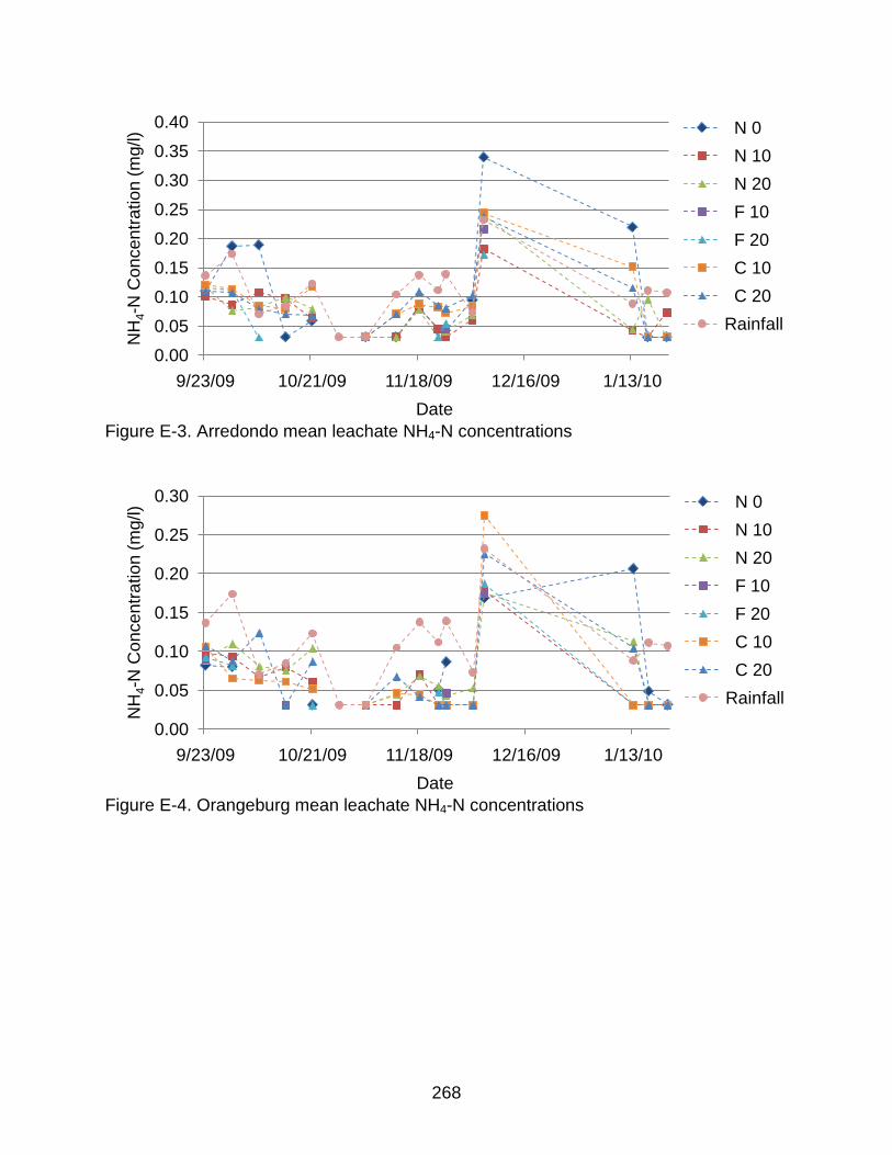
268
Figure E-3. Arredondo mean leachate NH4-N concentrations
Figure E-4. Orangeburg mean leachate NH4-N concentrations
0.00
0.05
0.10
0.15
0.20
0.25
0.30
0.35
0.40
9/23/09 10/21/09 11/18/09 12/16/09 1/13/10
NH
4-N
Con
cent
ratio
n (m
g/l)
Date
N 0N 10N 20F 10F 20C 10C 20
Rainfall
0.00
0.05
0.10
0.15
0.20
0.25
0.30
9/23/09 10/21/09 11/18/09 12/16/09 1/13/10
NH
4-N
Con
cent
ratio
n (m
g/l)
Date
N 0N 10N 20F 10F 20C 10C 20
Rainfall

269
Figure E-5. Arredondo mean runoff NO2+3-N Concentrations
Figure E-6. Orangeburg mean runoff NO2+3-N concentrations
0.00
0.10
0.20
0.30
0.40
0.50
0.60
9/23/09 10/21/09 11/18/09 12/16/09 1/13/10
NO
3-N
Con
cent
ratio
n (m
g/l)
Date
N 0N 10N 20F 10F 20C 10C 20
Rainfall
0.00
0.10
0.20
0.30
0.40
0.50
0.60
9/23/09 10/21/09 11/18/09 12/16/09 1/13/10
NO
3-N
Con
cent
ratio
n (m
g/l)
Date
N 0N 10N 20F 10F 20C 10C 20
Rainfall

270
Figure E-7. Arredondo mean leachate NO2+3-N concentrations
Figure E-8. Orangeburg mean leachate NO2+3-N concentrations
0.00
10.00
20.00
30.00
40.00
50.00
60.00
9/23/09 10/21/09 11/18/09 12/16/09 1/13/10
NO
3-N
Con
cent
ratio
n (m
g/l)
Date
N 0N 10N 20F 10F 20C 10C 20
Rainfall
0.00
2.00
4.00
6.00
8.00
10.00
12.00
14.00
16.00
9/23/09 10/21/09 11/18/09 12/16/09 1/13/10
NO
3-N
Con
cent
ratio
n (m
g/l)
Date
N 0N 10N 20F 10F 20C 10C 20
Rainfall

271
Figure E-9. Arredondo mean runoff TKN concentrations
Figure E-10. Orangeburg mean runoff TKN concentrations
0.00
2.00
4.00
6.00
8.00
10.00
12.00
9/23/09 10/21/09 11/18/09 12/16/09 1/13/10
TKN
Con
cent
ratio
n (m
g/l)
Date
N 0N 10N 20F 10F 20C 10C 20
Rainfall
0.00
2.00
4.00
6.00
8.00
10.00
12.00
9/23/09 10/21/09 11/18/09 12/16/09 1/13/10
TKN
Con
cent
rat (
mg/
l)
Date
N 0N 10N 20F 10F 20C 10C 20
Rainfall

272
Figure E-11. Arredondo mean leachate TKN concentrations
Figure E-12. Orangeburg mean leachate TKN concentration
0.00
1.00
2.00
3.00
4.00
5.00
6.00
7.00
9/23/09 10/21/09 11/18/09 12/16/09 1/13/10
TKN
Con
cent
ratio
n (m
g/l)
Date
N 0N 10N 20F 10F 20C 10C 20
Rainfall
0.00
0.20
0.40
0.60
0.80
1.00
1.20
1.40
9/23/09 10/21/09 11/18/09 12/16/09 1/13/10
TKN
Con
cent
ratio
n (m
g/l)
Date
N 0N 10N 20F 10F 20C 10C 20
Rainfall

273
Figure E-13. Arredondo mean runoff OP concentrations
Figure E-14. Orangeburg mean runoff OP concentrations
0
200
400
600
800
1000
1200
1400
9/23/09 10/21/09 11/18/09 12/16/09 1/13/10
OP
Con
cent
ratio
n (u
g/l)
Date
20 N 0
N 10
N 20
F 10
F 20
C 10
Rainfall
0
50
100
150
200
250
300
350
9/23/09 10/21/09 11/18/09 12/16/09 1/13/10
OP
Con
cent
ratio
n (u
g/l)
Date
N 0N 10N 20F 10F 20C 10C 20
Rainfall

274
Figure E-15. Arredondo mean leachate OP concentrations
Figure E-16. Orangeburg mean leachate OP concentrations
0
100
200
300
400
500
600
700
800
9/23/09 10/21/09 11/18/09 12/16/09 1/13/10
OP
Con
cent
ratio
n (u
g/l)
Date
N 0N 10N 20F 10F 20C 10C 20
Rainfall
0
50
100
150
200
250
300
9/23/09 10/21/09 11/18/09 12/16/09 1/13/10
OP
Con
cent
ratio
n (u
g/l)
Date
N 0N 10N 20F 10F 20C 10C 20
Rainfall

275
Figure E-17. Arredondo mean runoff pH
Figure E-18 Arredondo mean leachate pH
4.004.505.005.506.006.507.007.508.008.509.00
9/23/09 10/21/09 11/18/09 12/16/09 1/13/10
pH
Date
N 0N 10N 20F 10F 20C 10C 20
Rainfall
4.004.505.005.506.006.507.007.508.008.509.00
9/23/09 10/21/09 11/18/09 12/16/09 1/13/10
pH
Date
N 0N 10N 20F 10F 20C 10C 20
Rainfall

276
Figure E-19. Orangeburg mean runoff pH
Figure E-20. Orangeburg mean leachate pH
4.004.505.005.506.006.507.007.508.008.509.00
9/23/09 10/21/09 11/18/09 12/16/09 1/13/10
pH
Date
N 0N 10N 20F 10F 20C 10C 20
Rainfall
4.004.505.005.506.006.507.007.508.008.50
9/23/09 10/21/09 11/18/09 12/16/09 1/13/10
pH
Date
N 0N 10N 20F 10F 20C 10C 20
Rainfall

277
APPENDIX F ADDITIONAL COLUMN STUDY WATER QUALITY DATA
Leachate Column Results
Leachate samples collected from the column study were analyzed for analytes
listed in Table F-1 along with respective Practical Quantitation Limits (PQLs) and
Minimum Detection Limits (MDLs). Analyte concentrations of water matrix applied to
columns are also listed in Table F-1. Concentrations were determined by Inductively
Coupled Plasma-Atomic Emission Spectrometry (ICP-AES).
Total Phosphorus (TP)
Leachate concentrations of TP were highest for compost, followed in order by
Arredondo, fly ash, and Orangeburg columns. Concentrations of TP increased with
compost additions, more so on Arreodondo than Orangeburg though (Figure F-1).
However, fly ash incorporations did not produce noticeable increases in TP
concentrations.
Potassium (K)
Leachate concentrations of K were highest for compost, followed in order by fly
ash, Arredonodo, and Orangeburg columns. Incorporating higher fractions of both
amendments increased leachate K concentrations (Figure F-2).
Sodium (Na)
Leachate concentrations of Na were highest for compost, followed in order by fly
ash, Arredonodo, and Orangeburg columns. Incorporating higher fractions of both
amendments increased leachate Na concentrations (Figure F-3).

278
Magnesium (Mg)
Leachate concentrations of Mg were highest for fly ash, followed in order by
compost, Arredonodo, and Orangeburg columns. Incorporating higher fractions of both
amendments increased leachate Mg concentrations (Figure F-4).
Calcium (Ca)
Leachate concentrations of Ca were highest for fly ash, followed by compost and
both soils. Arredondo and Orangeburg Ca concentrations were essentially equal.
Incorporating higher fractions of both amendments increased leachate Ca
concentrations (Figure F-5).
Aluminum (Al)
Leachate concentrations of Al were highest for fly ash, followed in order by
Arredondo, compost and Orangeburg soils. Al concentrations fluctuated between
increases and decreases compared to the Arredondo column as both amendments
fractions increased. However, increased fractions of both amendments in Orangeburg
soils increased Al concentrations (Figure F-6).
Iron (Fe)
Leachate concentrations of Fe were highest for fly ash, followed in order by
compost, Arredondo, and Orangeburg soils. Increasing amendment fractions of
compost and fly ash increased Fe concentrations from Orangeburg soils (Figure F-7).
However, increasing compost fractions on Arredondo soils caused concentrations to dip
and then rise again, while increasing fly ash fractions did not increase Fe concentrations
except when comparing fly ash only to Arredondo only leachate concentrations.
Interactions between Arredondo and compost are attributed to the behavior of
concentrations from these mixtures.

279
Manganese (Mn)
Concentration fluctuations of Mn from increasing amendment fractions were
similar to Fe. Leachate concentrations were comparable for Arredondo and fly ash while
compost concentrations were lower and followed by Orangeburg. Increased fly ash
fractions in Arredondo caused concentrations to dip before increasing towards fly ash
only concentrations (Figure F-8). Similarly, Mn leachate concentrations from fly ash and
compost mixes with Orangeburg soil were lower than the Orangeburg only and
respective amendment only columns. This phenomenon was attributed to chemical
interactions between the fly ash and the soil. No trend was identified for increased
compost additions to Arredondo.
Zinc (Zn)
Leachate concentrations of Zn were highest for fly ash, followed by Orangeburg
and compost, which were essentially equal, and finally by Arredondo with the lowest
concentrations. Increasing compost fractions mixed with Arredondo increased Zn
concentrations, while increasing compost fractions mixed with Orangeburg caused Zn
concentrations to decrease for soil and amendment mixtures (Figure F-9). Increasing fly
ash additions to Arredondo decreased Zn concentrations until fly ash only
concentrations which were all greater than Arredondo only concentrations.
Copper (Cu)
Concentrations of Cu were greatest for fly ash, followed in order by compost,
Arredondo and Orangeburg. Increasing fractions of both amendments in both soils
eventually increased Cu concentrations (Figure F-10). However, no concentrations were
above the Cu MDL when increasing fly ash fractions into Orangeburg soils, except for
fly ash only.

280
Boron (B)
Concentrations of B were greatest for fly ash, followed in order by compost, and
both soils, which had concentrations below the B MDL. Increasing fractions of both
amendments in both soils eventually increased B concentrations (Figure F-11).
Concentrations increased more on Arredondo soils for each amendment than for similar
incorporations on Orangeburg soils. However, no concentrations were above the B MDL
when increasing compost fractions into Orangeburg soils, except for those from the
compost only column.
Nickel (Ni), Cadmium (Cd), and Lead (Pb)
All Ni concentrations were below the Ni MDL except those from fly ash only
columns and a single sample from a 0.1 fraction fly ash and Arredondo column (Figure
F-12). All sample concentrations of Cd and Pb were less than their respective MDLs.
Summary
Nearly all sample concentrations were greater than or equal to applied water
matrix concentrations. Concentrations of TP, K, Na, Ca, Mg, Cu, B and Fe increased for
both soils as both amendment fractions increased. Both amendments increased Al
concentrations while soil and amendment interactions resulted in non-linear
concentrations transitions between Arredondo and both amendment concentrations.
Interactions between Arredondo and both amendments also produced non-linear Fe
concentration changes as amendment fractions increased, while both soils increased
Fe concentrations from Orangeburg soils. Non-linear changes in Zn and Mn
concentrations were attributed to soil and amendment chemical interactions.

281
Fly Ash TCLP
A Toxicity Characteristic Leaching Procedure (TCLP) was conducted
concentrations of several metals on a sample of fly ash used in this study. Additional
metals were also included in the analysis. Results are presented in Table F-2. None of
the eight TCLP metals exceeded their respective toxicity limits (EPA, 2004). Thus, the
fly ash was determined not to be toxic by TCLP analysis.
Table F-1. Practical Quantitation Limits (PQL), Minimum Detection Limits (MDL) and applied water matrix concentrations.
Analyte Units PQL MDL Water Matrix Concentration Al (mg/l) 0.5000 0.1250 < 0.1250#
B (mg/l) 0.6000 0.1500 < 0.1500 Ca (mg/l) 0.2500 0.0525 13.0336 Cd (mg/l) 0.5000 0.1250 < 0.1250 Cu (mg/l) 0.0500 0.0125 < 0.0125 Fe (mg/l) 0.0500 0.0125 E0.0184 K (mg/l) 5.0000 1.2500 < 1.2500 Mg (mg/l) 0.1000 0.0250 9.1407 Mn (mg/l) 0.0500 0.0125 < 0.0125 Na (mg/l) 5.0000 1.2500 5.5720 Ni (mg/l) 0.0500 0.0125 < 0.0125 P (mg/l) 0.1000 0.0250 < 0.0250 Pb (mg/l) 0.1000 0.0250 < 0.0250 Zn (mg/l) 0.0500 0.0125 E 0.0259 E: Reported values were greater than the MDL but less than the PQL. # Values were reported as less than MDL.

282
Table F-2. Toxicity Characteristic Leaching Protocol results for fly ash sample, with corresponding lab Practical Quantitation Level (PQL), Minimum Detection Level (MDL), and toxicity limits.
Parameter Fly ash result (mg/kg)
PQL (mg/kg)
MDL (mg/kg)
Toxicity limit (EPA, 2004) (mg/kg)
Antimony (Sb) 3.1 0.98 0.16 Arsenic (As) 31 0.33 0.3 100
Barium (Ba) 160 0.065 0.037 2000 Beryllium (Be) 4.1 0.0098 0.0028
Cadmium (Cd) 0.15 0.02 0.0041 20 Chromium (Cr) 19 0.13 0.077 100 Cobalt (Co) 11 0.13 0.023
Copper (Cu) 49 0.13 0.07 Lead (Pb) 15 0.23 0.066 100
Mercury (Hg) 0.0012 0.0065 0.00091 4 Nickel (Ni) 21 0.21 0.063
Selenium (Se) 2.5 0.65 0.24 20 Silver (Ag) 0.039 0.13 0.039 100 Thallium (Tl) 0.17 0.81 0.17
Tin (Sn) 2.7 0.65 0.14 Vanadium (V) 63 0.049 0.011 Zinc (Zn) 28 0.33 0.24
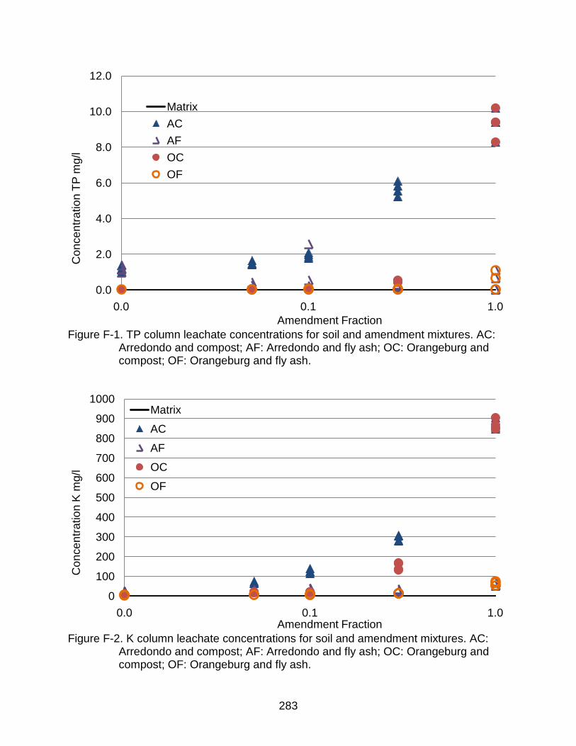
283
Figure F-1. TP column leachate concentrations for soil and amendment mixtures. AC:
Arredondo and compost; AF: Arredondo and fly ash; OC: Orangeburg and compost; OF: Orangeburg and fly ash.
Figure F-2. K column leachate concentrations for soil and amendment mixtures. AC:
Arredondo and compost; AF: Arredondo and fly ash; OC: Orangeburg and compost; OF: Orangeburg and fly ash.
0.0
2.0
4.0
6.0
8.0
10.0
12.0
0.0 0.1 1.0
Con
cent
ratio
n TP
mg/
l
Amendment Fraction
MatrixACAFOCOF
0
100
200
300
400
500
600
700
800
900
1000
0.0 0.1 1.0
Con
cent
ratio
n K
mg/
l
Amendment Fraction
Matrix
AC
AF
OC
OF

284
Figure F-3. Na column leachate concentrations for soil and amendment mixtures. AC:
Arredondo and compost; AF: Arredondo and fly ash; OC: Orangeburg and compost; OF: Orangeburg and fly ash.
Figure F-4. Mg column leachate concentrations for soil and amendment mixtures. AC: Arredondo and compost; AF: Arredondo and fly ash; OC: Orangeburg and compost; OF: Orangeburg and fly ash.
0
50
100
150
200
250
0.0 0.1 1.0
Con
cent
ratio
n N
a m
g/l
Amendment Fraction
Matrix
AC
AF
OC
OF
0
20
40
60
80
100
120
0.0 0.1 1.0
Con
cent
ratio
n M
g m
g/l
Amendment Fraction
Matrix
AC
AF
OC
OF

285
Figure F-5. Ca column leachate concentrations for soil and amendment mixtures. AC: Arredondo and compost; AF: Arredondo and fly ash; OC: Orangeburg and compost; OF: Orangeburg and fly ash.
Figure F-6. Al column leachate concentrations for soil and amendment mixtures. AC: Arredondo and compost; AF: Arredondo and fly ash; OC: Orangeburg and compost; OF: Orangeburg and fly ash.
0
100
200
300
400
500
600
700
800
0.0 0.1 1.0
Con
cent
ratio
n C
a m
g/l
Amendment Fraction
Matrix
AC
AF
OC
OF
0.0
10.0
20.0
30.0
40.0
50.0
60.0
70.0
0.0 0.1 1.0
Con
cent
ratio
n A
l mg/
l
Amendment Fraction
Matrix
AC
AF
OC
OF

286
Figure F-7. Fe column leachate concentrations for soil and amendment mixtures. AC: Arredondo and compost; AF: Arredondo and fly ash; OC: Orangeburg and compost; OF: Orangeburg and fly ash.
Figure F-8. Mn column leachate concentrations for soil and amendment mixtures. AC: Arredondo and compost; AF: Arredondo and fly ash; OC: Orangeburg and compost; OF: Orangeburg and fly ash.
0.0
1.0
2.0
3.0
4.0
5.0
6.0
7.0
8.0
9.0
0.0 0.1 1.0
Con
cent
ratio
n Fe
mg/
l
Amendment Fraction
Matrix
AC
AF
OC
OF
0.0
0.1
0.2
0.3
0.4
0.5
0.6
0.7
0.8
0.9
1.0
0.0 0.1 1.0
Con
cent
ratio
n M
n m
g/l
Amendment Fraction
Matrix
AC
AF
OC
OF

287
Figure F-9. Zn column leachate concentrations for soil and amendment mixtures. AC:
Arredondo and compost; AF: Arredondo and fly ash; OC: Orangeburg and compost; OF: Orangeburg and fly ash.
Figure F-10. Cu column leachate concentrations for soil and amendment mixtures. AC:
Arredondo and compost; AF: Arredondo and fly ash; OC: Orangeburg and compost; OF: Orangeburg and fly ash.
0.0
0.1
0.2
0.3
0.4
0.5
0.6
0.7
0.8
0.0 0.1 1.0
Con
cent
ratio
n Zn
mg/
l
Amendment Fraction
Matrix
AC
AF
OC
OF
0.00
0.05
0.10
0.15
0.20
0.25
0.30
0.35
0.40
0.45
0.0 0.1 1.0
Con
cent
ratio
n C
u m
g/l
Amendment Fraction
Matrix
AC
AF
OC
OF

288
Figure F-11. B column leachate concentrations for soil and amendment mixtures. AC:
Arredondo and compost; AF: Arredondo and fly ash; OC: Orangeburg and compost; OF: Orangeburg and fly ash.
Figure F-12. Ni column leachate concentrations for soil and amendment mixtures. AC:
Arredondo and compost; AF: Arredondo and fly ash; OC: Orangeburg and compost; OF: Orangeburg and fly ash.
0.0
0.5
1.0
1.5
2.0
2.5
3.0
3.5
4.0
0.0 0.1 1.0
Con
cent
ratin
o B
mg/
l
Amendment Fraction
Matrix
AC
AF
OC
OF
0.00
0.02
0.04
0.06
0.08
0.10
0.12
0.14
0.0 0.1 1.0
Con
cent
ratio
n N
i mg/
l
Amendment Fraction
Matrix
AC
AF
OC
OF

289
Figure F-13. Cd column leachate concentrations for soil and amendment mixtures. AC:
Arredondo and compost; AF: Arredondo and fly ash; OC: Orangeburg and compost; OF: Orangeburg and fly ash.
Figure F-14. Pb column leachate concentrations for soil and amendment mixtures. AC:
Arredondo and compost; AF: Arredondo and fly ash; OC: Orangeburg and compost; OF: Orangeburg and fly ash.
0.00
0.01
0.02
0.03
0.04
0.05
0.06
0.07
0.0 0.1 1.0
Con
cent
ratio
n C
d m
g/l
Amendment Fraction
Matrix
AC
AF
OC
OF
0.000
0.002
0.004
0.006
0.008
0.010
0.012
0.014
0.0 0.1 1.0
Con
cent
ratio
n P
b m
g/l
Amendment Fraction
Matrix
AC
AF
OC
OF
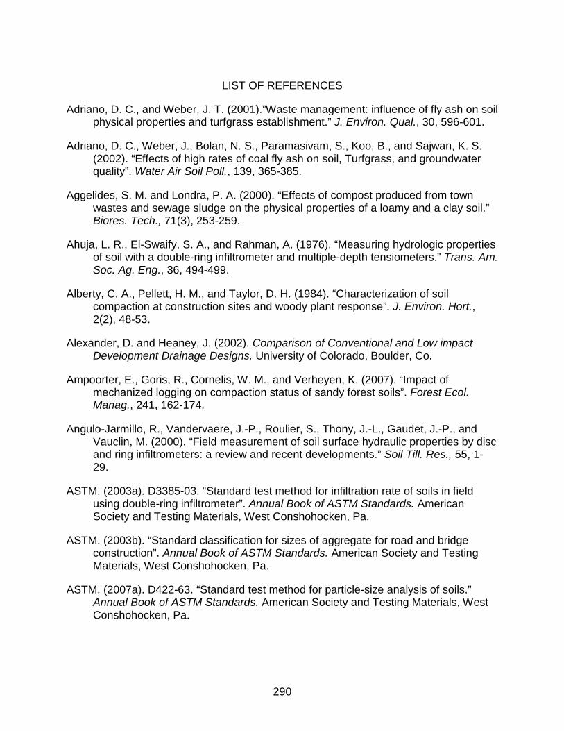
290
LIST OF REFERENCES
Adriano, D. C., and Weber, J. T. (2001).”Waste management: influence of fly ash on soil physical properties and turfgrass establishment.” J. Environ. Qual., 30, 596-601.
Adriano, D. C., Weber, J., Bolan, N. S., Paramasivam, S., Koo, B., and Sajwan, K. S. (2002). “Effects of high rates of coal fly ash on soil, Turfgrass, and groundwater quality”. Water Air Soil Poll., 139, 365-385.
Aggelides, S. M. and Londra, P. A. (2000). “Effects of compost produced from town wastes and sewage sludge on the physical properties of a loamy and a clay soil.” Biores. Tech., 71(3), 253-259.
Ahuja, L. R., El-Swaify, S. A., and Rahman, A. (1976). “Measuring hydrologic properties of soil with a double-ring infiltrometer and multiple-depth tensiometers.” Trans. Am. Soc. Ag. Eng., 36, 494-499.
Alberty, C. A., Pellett, H. M., and Taylor, D. H. (1984). “Characterization of soil compaction at construction sites and woody plant response”. J. Environ. Hort., 2(2), 48-53.
Alexander, D. and Heaney, J. (2002). Comparison of Conventional and Low impact Development Drainage Designs. University of Colorado, Boulder, Co.
Ampoorter, E., Goris, R., Cornelis, W. M., and Verheyen, K. (2007). “Impact of mechanized logging on compaction status of sandy forest soils”. Forest Ecol. Manag., 241, 162-174.
Angulo-Jarmillo, R., Vandervaere, J.-P., Roulier, S., Thony, J.-L., Gaudet, J.-P., and Vauclin, M. (2000). “Field measurement of soil surface hydraulic properties by disc and ring infiltrometers: a review and recent developments.” Soil Till. Res., 55, 1-29.
ASTM. (2003a). D3385-03. “Standard test method for infiltration rate of soils in field using double-ring infiltrometer”. Annual Book of ASTM Standards. American Society and Testing Materials, West Conshohocken, Pa.
ASTM. (2003b). “Standard classification for sizes of aggregate for road and bridge construction”. Annual Book of ASTM Standards. American Society and Testing Materials, West Conshohocken, Pa.
ASTM. (2007a). D422-63. “Standard test method for particle-size analysis of soils.” Annual Book of ASTM Standards. American Society and Testing Materials, West Conshohocken, Pa.

291
ASTM (2007b). “Standard test methods for laboratory compaction characteristics of soil using standard effort (12 400 ft-lbf/ft3 (600 kN-m/m3))”. Annual Book of ASTM Standards. American Society and Testing Materials, West Conshohocken, Pa.
ASTM. (2008). “Standard specification for coal fly ash and raw or calcined natural pozzolan for use in concrete”. Annual Book of ASTM Standards. American Society and Testing Materials, West Conshohocken, Pa.
Baba, A. and Kaya, A. (2004). “Leaching characteristics of fly ash from thermal power plants of Soma and Tuncbilek, Turkey”. Env. Monit. Assessment. 91, 171-181.
Bardin, J.-P., Gautier, A., Barraud, S., and Chocat, B. (2004). “The purification performance of infiltration basin fitted with pretreatment facilities: a case study”. Water Sci. Technol., 43(5), 119-128.
Barraud, S., Gautier, A., Bardin, J. P., and Riou, V. (1999). “The impact of intentional stormwater infiltration on soil and groundwater”. Water Sci. Technol., 39(2), 185-192.
Barrett, M. E., Irish, L. B., Malina, J. F., and Charbeneau, R. J. (1998). “Characterization of highway runoff in Austin, Texas, area.” J. Environ. Eng., 124(2), 131-137.
Bartens, J., Day, S. D., Harris, J. R., Dove, J. E., and Wynn, T. M. (2008). “Can urban tree roots improve infiltration through compacted subsoils for stormwater management?” J. Environ. Qual., 37, 2048-2057.
Bayat, O. (1997). “Characterization of Turkish fly ashes”. Fuel, 77(9-10), 1059-1066.
Bin-Shafique, S., Benson, C. H., Edil, T. B., and Hwang, K. (2006). “Leachate concentration from water leach and column leach tests on fly ash-stabilized soils”. Environ. Eng. Sci., 23(1), 53-67.
Blake, G. R. and Hartge, K. H. (1986). Bulk Density. In Methods of Soil Analysis, Part I, ASA Monograph, 9, 363-375. A. Klute ed. Madison, Wisconsin.
Booth, D. B., Hartley, D., and Jackson, C. R. (2002). “Forest cover, impervious-surface area, and the mitigation of stormwater impacts”, J. Am. Wat. Resour. As., 38(3), 835-845.
Bouwer, H., Ludke, J., and Rice, R. C. (2001). “Sealing pond bottoms with muddy water.” Ecol. Eng., 18, 233-238.
Breland, T. A. and Hansen, S. (1995). “Nitrogen mineralization and microbial biomass as affected by soil compaction”. Soil Biol. Biochem., 28(4-5), 655-663.
Campbell, D. J., Fox, W. E., Aitken, R. L., and Bell, L. C. (1983). “Physical characteristics of sands amended with fly ash”. Aust. J. Soil Res., 21, 147-154.
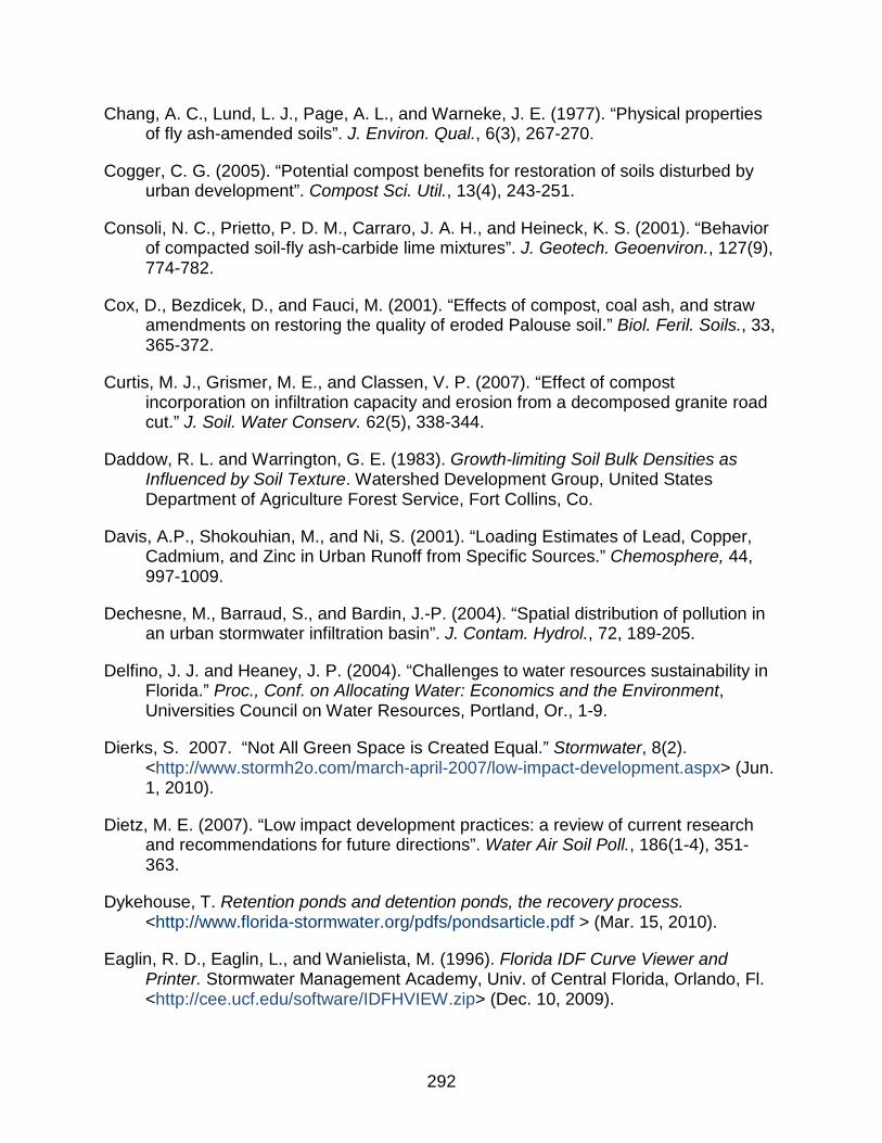
292
Chang, A. C., Lund, L. J., Page, A. L., and Warneke, J. E. (1977). “Physical properties of fly ash-amended soils”. J. Environ. Qual., 6(3), 267-270.
Cogger, C. G. (2005). “Potential compost benefits for restoration of soils disturbed by urban development”. Compost Sci. Util., 13(4), 243-251.
Consoli, N. C., Prietto, P. D. M., Carraro, J. A. H., and Heineck, K. S. (2001). “Behavior of compacted soil-fly ash-carbide lime mixtures”. J. Geotech. Geoenviron., 127(9), 774-782.
Cox, D., Bezdicek, D., and Fauci, M. (2001). “Effects of compost, coal ash, and straw amendments on restoring the quality of eroded Palouse soil.” Biol. Feril. Soils., 33, 365-372.
Curtis, M. J., Grismer, M. E., and Classen, V. P. (2007). “Effect of compost incorporation on infiltration capacity and erosion from a decomposed granite road cut.” J. Soil. Water Conserv. 62(5), 338-344.
Daddow, R. L. and Warrington, G. E. (1983). Growth-limiting Soil Bulk Densities as Influenced by Soil Texture. Watershed Development Group, United States Department of Agriculture Forest Service, Fort Collins, Co.
Davis, A.P., Shokouhian, M., and Ni, S. (2001). “Loading Estimates of Lead, Copper, Cadmium, and Zinc in Urban Runoff from Specific Sources.” Chemosphere, 44, 997-1009.
Dechesne, M., Barraud, S., and Bardin, J.-P. (2004). “Spatial distribution of pollution in an urban stormwater infiltration basin”. J. Contam. Hydrol., 72, 189-205.
Delfino, J. J. and Heaney, J. P. (2004). “Challenges to water resources sustainability in Florida.” Proc., Conf. on Allocating Water: Economics and the Environment, Universities Council on Water Resources, Portland, Or., 1-9.
Dierks, S. 2007. “Not All Green Space is Created Equal.” Stormwater, 8(2). <http://www.stormh2o.com/march-april-2007/low-impact-development.aspx> (Jun. 1, 2010).
Dietz, M. E. (2007). “Low impact development practices: a review of current research and recommendations for future directions”. Water Air Soil Poll., 186(1-4), 351-363.
Dykehouse, T. Retention ponds and detention ponds, the recovery process. <http://www.florida-stormwater.org/pdfs/pondsarticle.pdf > (Mar. 15, 2010).
Eaglin, R. D., Eaglin, L., and Wanielista, M. (1996). Florida IDF Curve Viewer and Printer. Stormwater Management Academy, Univ. of Central Florida, Orlando, Fl. <http://cee.ucf.edu/software/IDFHVIEW.zip> (Dec. 10, 2009).

293
Eghball, B. and Power, J. F. (1999). “Phosphorus- and nitrogen-based manure and compost applications: corn production and soil phosphorus”. Soil Sci. Soc. Am. J., 63, 895-901.
Eghball, B. (2002). “Soil properties as influenced by phosphorus- and nitrogen-based manure and compost applications”. Agron. J., 94(1), 128-135.
Eghball, B. (2003). “Leaching of phosphorus fractions following manure or compost application”. Commun. Soil Sci. Plan., 34(19-20), 2803-2815.
Eneji, A. E., Honna, T., Yamamoto, S., Masuda, T., Endo, T., and Irshad, M. (2003). “Changes in humic substances and phosphorus fractions during composting”. Commun. Soil Sci. Plan., 34(15-16), 2303-2314.
Energy Information Administration (EIA). (2008). Annual Energy Outlook 2008. Energy Information Administration, Department of Energy, Washington, DC.
Environmental Protection Agency (EPA). (1996). Overview of the Storm Water Program. Office of Water, EPA, Washington, DC.
Environmental Protection Agency (EPA). (1999a). Low-Impact Development Design Strategies: An Integrated Design Approach. Office of Water, EPA, Washington, DC.
Environmental Protection Agency (EPA). (2000b). Stormwater Phase II Final Rule: Small MS4 Stormwater Program Overview. Office of Water, EPA, Washington, DC.
Environmental Protection Agency (EPA). (2000c). Stormwater Phase II Final Rule: Post-construction Runoff Control Minimum Control Measure. Office of Water, EPA, Washington, DC.
Environmental Protection Agency (EPA). (2004). “Test Methods for Evaluating Solid Waste,” SW-846, 4rd Ed., Office of Solid Waste and Emergency Response, Washington, DC.
Environmental Protection Agency (EPA). (2007). Reducing Stormwater Costs through Low Impact Development (LID) Strategies and Practices. Office of Water, EPA, Washington, DC.
Environmental Protection Agency (EPA). (2009a). National Water Quality Inventory: Report to Congress. 2004 Reporting Cycle. Office of Water, EPA, Washington, DC.
Environmental Protection Agency (EPA). (2009b). National Primary Drinking Water Regulations. Office of Water, EPA, Washington, DC.
294
Filcheva, E.G. and Tsadilas, C.D. (2002). “Influence of clinoptilolite and compost on soil properties”. Commun. Soil Sci. Plan., 33(3-4), 595-607.
Florida Department of Environmental Protection (FDEP). (1988). “Chapter 6: Stormwater and Erosion and Sediment Control Best Management Practices for Developing Areas”. The Florida Development Manual: A Guide to Sound Land and Water Management. FDEP, Tallahassee, Fl.
Florida Department of Environmental Protection (FDEP). (1989). Criteria for the Production and Use of Compost Made from Solid Waste. Florida Administrative Code (FAC), Chapter 62-709. FDEP, Tallahassee, Fl.
Florida Department of Environmental Protection (FDEP). (2008). “Statewide stormwater treatment rule development background.” Statewide Stormwater Treatment Rule Development <http://p2000.dep.state.fl.us/water/wetlands/erp/rules/stormwater/ background.htm> (May 5, 2010).
Gangloff, W. J., Ghodrati, M., Sims, J. T., and Vasilas, B. L. (2000). “Impact of fly ash amendment and incorporation method on hydraulic properties of a sandy soil”. Water Air Soil Poll., 119, 231-245.
Gaskin, J. W., Risse, L. M., Kastner, J. R., and McLaurin, W. J. (2005). “Evaluating onsite beneficial reuse of ground engineered wood wastes from residential construction”. T. ASAE. 48(5), 1731-1738.
Gee, G. W. and Bauder, J. W. (1986). Particle-size Analysis. In Methods of Soil Analysis, Part I, ASA Monograph, 9, 383-411. A. Klute ed. Madison, Wisconsin.
GeoSyntech Consultants and Wright Water Engineers, Inc. (GC & WWE). (2008). Analysis of Treatment System Performance: International Stormwater Best Management Practices (BMP)Database [1999-2008].
Gill, W. R. and Vanden Berg, G. E. (1968). “Soil compaction”. In Soil Dynamics in Tillage and Traction, Agricultural Handbook No. 316. US Government Printing Office, Washington, DC, 430-446.
Gilley, J. E. and Eghball, B. (2002). “Residual effects of compost and fertilizer applications on nutrients in runoff“. T. ASAE., 45(6), 1905-1910.
Glanville, T. D., Persyn, R. A., Richard, T. L., Laflen, J. M., and Dixon, P. M. (2004). “Environmental effects of applying composted organics to new highway embankments: part 2. water quality”. T. ASAE. 47(2), 471-478.
Graecen, E. L. and Sands, R. (1980). “Compaction of forest soils. A review”. Aust. J. Soil Res., 18, 163-189.
Green W. H., and Ampt, G.A. (1911). “Studies on soil physics, part I, the flow of air and water through soils”. J. Agric. Sci., 4(1), 1-24.

295
Gregory, J. H. (2004). “Stormwater infiltration at the scale of an individual residential lot in North Central Florida.” MS Thesis, Univ. of Florida, Gainesville, Fl.
Gregory, J. H., Dukes, M. D., Jones, P. H., and Miller, G. L. (2006). “Effect of urban soil compaction on infiltration rate”. J. Soil Water Conserv., 61(3), 117-124.
Gregory, J. H., Dukes, M. D., Miller, G. L., and Jones, P. H. (2005). “Analysis of double-ring infiltration techniques and development of a simple automatic water delivery system.” Applied Turfgrass Science. May, 2005.
Guo, J. C. Y. and Hughes, W. (2001). “Storage volume and overflow risk for infiltration basin design”. J. Irrig. Drain. Eng., 127(3), 170-175.
Gupta, A. K., S. Dwivedi, S. Sinha, R. D. Tripathi, U. N. Rai, and S. N. Singh. (2007). “Metal accumulation and growth performance of Phaseolus vulgaris grown in fly ash amended soil.” Bioresource Technol., 98, 3404-3407.
Gupta, S. C. and Larson, W. E. (1979). “Estimating soil water retention characteristics from particle size distribution, organic matter percent, and bulk density.” Water Resour. Res., 15(6), 1633-1635.
Hansen, S., Maehlum, J. E., and Bakken, L. R. (1993). “N2O and CH4 fluxes in soil influences by fertilization and tractor traffic”. Soil Biol. Biochem., 25(5), 621-630.
Hamza, M. A. and Anderson, W. K. (2005). “Soil compaction in cropping systems: a review of the nature, causes and possible solutions”. Soil Till. Res., 82, 121-145.
Harper, H. and Baker, D. (2007). “Evaluation of current stormwater design criteria within the state of Florida.” Final Report. Prepared by Environmental Research & Design. Orlando, FL.
Hatt, B.E., Fletcher, T.D., Walsh, C.J., and Taylor, S.L. (2006). “The influence of urban density and drainage infrastructure on the concentrations and loads of pollutants in small streams.” Environ. Manage., 34(1), 112-124.
Hawkins, R. H. (1993). “Asymptotic determination of runoff curve numbers from data”. J. Irr. Drain. Eng., 119(2), 334-345.
He, W., Wallinder, I. O., and Leygraf, C. (2001). “A laboratory study of copper and zinc runoff during first flush and steady-state conditions.” Corrosion Science, 43, 127-146.
Heiri, O., Lotter, A. F., and Lemcke, G. (2001). “Loss on ignition as a method for estimating organic and carbonate content in sediments: reproducibility and comparability of results.” J. Paleolimnology, 25, 101-110.
Hillel, D. (1998). Environmental Soil Physics. Academic Press, San Diego, CA.

296
Hood, M. J., Clausen, J. C., and Warner, G. S. (2007). “Comparison of stormwater lag times for low impact and traditional residential development”. J. Am. Water Resour. As., 43(4), 1036-1046.
Hower, J. C., Robertson, J. D., Thomas, G. A., Wong, A. S., Schram, W. H., Graham, U. M., Rathbone, R. F., and Robl, T. L. (1995). “Characterization of fly ash from Kentucky power plants”. Fuel. 75(4), 403-411.
Hunt, W. F., Apperson, C. S., Kennedy, S. G., Harrison, B. A., and Lord, W. G. (2006). “Occurrence and relative abundance of mosquitoes in stormwater retention facilities in North Carolina, USA.” Water Sci. Technol., 54(6-7), 315-321.
Jaber, F. H., Shukla, S., Stoffella, P. J., Obreza, T. A., and Hanlon, E. A. (2005). “Impact of organic amendments on groundwater nitrogen concentrations for sandy and calcareous soils”. Compost Sci. Util., 13(3), 194-202.
Jaber, F. H., Shukla, S., Hanlon, E. A., Stoffella, P. J., Obreza, T. A., Bryan, H. H. (2006). “Groundwater phosphorus and trace element concentrations from organically amended sandy and calcareous soils of Florida”. Compost Sci. Util., 14(1), 6-15.
Jastrow, J. D., and R. M. Miller. 1991. “Methods for assessing the effects of biota on soil structure.” Agric. Ecosystems Environ., 34, 279-303.
Kalra, N., Jain, M. C., Joshi, H. C., Choudhary, R., Harit, R. C., Vatsa, B. K., Sharma, S. K., and Kumar, V. (1998). “Flyash as a soil conditioner and fertilizer.” Bioresource Technol., 64, 163-167.
Katsvairo, T. W., D. L. Wright, J. J. Marois, D. L. Hartzog, K. B. Balkcom, P. P. Wiatrak, and J. R. Rich. (2007). “Cotton roots, earthworms, and infiltraiton characteristics in sod-peanut-cotton cropping systems.” Agronomy J., 99, 390-398.
Kaufman, M. G., Bray, A. K., Makowski, D., and Walker, E. D. (2005). “Mosquito production from storm water catchment systems in Michigan”. Proc. World Water and Environmental Resources Conference 2005, ASCE, Reston, Va.
Khandekar, M. P., Bhide, A. D., and Sajwan, K. S. (1997). “Trace elements in Indian coal and coal fly ash”. In Biogeochemistry of Trace Elements in Coal and Coal Combustion Byproducts. K. S. Sajwan et al. (eds.), Kluwer Academic/Plenum Publishers, New York, NY., 99-114.
Kosugi, K. (1996). “Lognormal distribution model for unsaturated soil hydraulic properties.” Wat. Resour. Res., 32(9), 2697-2703.
Kozlowski, T. T. (1999). “Soil Compaction and Growth of Woody Plants.” Scand. J. Forest Res., 14, 596-619.

297
Lai, J. and Ren, L. (2007). “Assessing the size dependency of measured hydraulic conductivity using double-ring infiltrometers and numerical simulation.” Soil Sci. Soc. Am. J.,71, 1667-1675.
Landschoot, P. (2002). Using composts to improve turf performance. Department of Crop and Soil Science, Penn State University, State College, Pa.
Landschoot P. and McNitt A. (1994). “Improving turf with compost”. BioCycle. 35 (10), 54-57.
Langmaack, M., Schrader, S., Rapp-Bernhardt, U., and Kotzke, K. (1999). “Quantitative analysis of earthworm burrow systems with respect to biological soil-structure regeneration after soil compaction”. Biol. Fert. Soils, 28, 219-229.
Le Coustumer, S., Moura, P., Barraud, S., Clozel, B., and Varnier, J.-C. (2007). “Temporal evolution and spatial distribution of heavy metals in a stormwater infiltration basin-estimation of the mass of trapped pollutants”. Water Sci. Technol., 56(12), 93-100.
Lee, J.G. and J.P. Heaney. (2003). “Estimation of urban imperviousness and its impacts on storm water systems.”, J. Water Res. Pl., 129(5), 419-426.
Lee, J. H. and Bang, K. W. (2000). “Characterization of urban stormwater runoff.” Wat. Res., 34(6), 1773-1780
Lee, J. G., Heaney, J. P., and Pack, C. A. (2010). “Frequency methodology for evaluating urban and highway storm-water quality control infiltration BMPs”. J. Water Res. Pl., ASCE, 136(2), 237-247.
Livingston, E. (2000). “Lessons Learned about Successfully Using Infiltration Practices.” Proc., National Conference on Tools for Urban Water Resource Management and Protection. Environmental Protection Agency, Washington, DC., 81-96.
Livingston, E. (2001). Stormwater Management in Florida: The Past, the Present, and the Future. Bureau of Watershed Management, Florida Department of Environmental Protection, Tallahassee, Fl.
Livingston, E. H., Horner, R. R., May, C., and Maxted, J. (2006). “BMPs, impervious cover, and biological integrity of small streams.” Proc., 2nd Biennial Stormwater Res. Symp., Southwest Florida Water Management District, Orlando, Fl., 13-35.
Logsdon, S. D., and Jaynes, D. B. (1996). “Spatial variability of hydraulic conductivity in a cultivated field at different times.” Soil Sci. Soc. Am. J., 60, 703-709.
Loper, S. (2009). “Effects of compost and tillage on soils and nutrient losses in a simulated residential landscape”. MS thesis, Univ. of Florida, Gainesville, Fl.

298
McCuen, R. H. and G. E. Moglen. 1988. “Multicriterion stormwater management methods.” J. Water Res. Plng. Mgmt., 114(4), 414-431.
Meek, B. D., E. R. Rechel, L. M. Carter, W. R. DeTar, and A. L. Urie. 1992. “Infiltration rate of a sandy loam soil: effects of traffic, tillage, and plant roots.“ Soil Sci. Soc. Am. J., 56, 908--913.
Minasny, B. and McBratney, A. B. (2007). “Estimating the water retention shape parameter from sand and clay content.” Soil Sci. Soc. Am. J., 71, 1105-1110.
Naseri, A. A., Jafari, S. and Alimohammadi, M. (2007). “Soil compaction due to sugarcane (Saccharum officinarum) mechanical harvesting and the effects of subsoiling on the improvement of soil physical properties”. J. Appl. Sci., 7(23), 3639-3648.
Nathan, Y., Dvorachek, M., Pelly, I., and Mimran, U. (1999). “Characterization of coal fly ash from Israel”. Fuel. 78, 205-213.
National Organic Standards Board. (2002). Compost Task Force Recommendation. Agricultural Marketing Service, United States Department of Agriculture, Washington, DC.
National Resource Council (NRC). (2008). Urban Stormwater in the United States. National Academies Press, Washington, DC.
Natural Resource Conservation Service (NRCS). 1986. “Technical Release-55: Urban hydrology for small watersheds. U.S. Department of Agriculture, Natural Resource Conservation Service.” 2nd Ed.
Natural Resource Conservation Service (NRCS). 1993. “Examination and description of soils”. Soil Survey Manual, Chapter 3. Washington, DC.
Natural Resource Conservation Service (NRCS). 1998. “Composting”. Backyard Conservation: It’ll Grow on You. National Association of Conservation Districts, Washington, DC.
Obreza, T., Clark, M., Boman, B., Borisova, T., Cohen, M., Dukes, M., Frazer, T., Hanlon, E., Havens, K., Martinez, C., Migliaccio, K., Shukla, S., and Wright, A. (2010). “A guide to EPA’s proposed numeric nutrient water quality criteria for Florida.” SL316. Institute of Food and Agricultural Sciences, University of Florida, Gainesville, FL.
Olson, E. C. S., Chanasyk, D. S., and Miller, J. J. (2005). “Effects of fresh versus composted manure on hydrologic response from cropland”. T. ASAE., 48(6), 2163-2168.

299
Pandey, C. (2005). “Effects of water table management and organic amendment on water quantity and quality in south Florida”. PhD dissertation, Univ. of Florida, Gainesville, Fl.
Parton, W. J., Schimel, D. S., Cole, C. V., and Ojima, D. S. (1987). “Analysis of factors controlling soil organic matter levels in great plains grasslands”. Soil Sci. Soc. Am. J., 51, 1173-1179.
Pathan, S. M., Aylmore, L. A. G., and Colmer, T. D. (2002). “Reduced leaching of nitrate, ammonium, and phosphorus in a sandy soil by fly ash amendment. Aust. J. Soil Res., 40, 1201-1211.
Pathan, S. M., Aylmore, L. A. G., and Colmer, T. D. (2003). “Properties of several fly ash materials in relation to use as soil amendments”. J. Environ. Qual., 32, 687-693.
Paul, M.J. and Meyer, J. L.(2001). “Streams in the urban landscape.” Annual Review of Ecological Systems, 32, 333-365.
Pitt, R., Clark, S., and Field, R. (1999a). “Groundwater contamination potential from stormwater infiltration practices”. Urb. Wat., 1(3), 217-236.
Radford, B. J., Yule, D. F., McGarry, D., and Playford, C. (2007). “Amelioration of soil compaction can take 5 years on a Vertisol under no till in the semi-arid subtropics”. Soil Till. Res., 97, 249-255.
Ram, L. C., Srivastava, N. K., Tripathi, R. C., Thakur, S. K., Sinha, A. K., Jha, S. K., Masto, R. E., and Mitra, S. (2007). “Leaching behavior of lignite fly ash with shake and column tests.” Environ. Geol., 51, 1119-1132.
Randrup, T. B. and Lichter, J. M. (2001). “Measuring soil compaction on construction sites: a review of surface nuclear gauges and penetrometers”. J. Arboriculture, 27(3), 109-117.
Raper, R. L. and Kirby, J. M. (2006). “Soil compaction: how to do it, undo it, and avoid doing it”. ASABE Distinguished Lecture Series, 30, 1-14.
Reddy, K. J. (1999). “Coal fly ash chemistry and carbon dioxide infusion process to enhance its utilization”. in Biogeochemistry of trace elements in coal and coal combustion by-products. K. S. Sajwan et al. (eds.), Kluwer Academic/Plenum Publishers, New York, NY., 133-144.
Ruser, R., Flessa, H., Russow, R., Schmidt, G., Buegger, F., and Munch, J. C. (2006). “Emission of N2O, N2, and CO2 from soil fertilized with nitrate: effect of compaction, soil moisture and rewetting”. Soil Biol. Biochem., 38, 263-274.

300
Sansalone, J. J. and Cristina, C.M. (2004). “First flush concepts for suspended and dissolved solids in small impervious watersheds.” J. Environ. Eng., 130(11), 1301-1314.
Sansalone, J., Kuang, X., and Ranieri, V. (2008). “Permeable pavement as a hydraulic and filtration interface for urban drainage”. J. Irrig. Drain. Eng., 134(5), 666-674.
Sarkar, A., Rano, R., Mishra, K. K., and Sinha, I. N. (2005). “Particle distribution profile of some Indian fly ash – a comparative study to assess their possible uses”. Fuel Process Technol., 86, 1221-1238.
Sartain, J. B. (2007). “General recommendations for fertilization of turfgrasses on Florida soils”. SL21, Institute of Food and Agricultural Sciences, University of Florida, Gainesville, FL.
SAS Institute, Inc. (2001). The SAS System for Windows (Release 9.1), Cary, NC.
Sidiras, N. and Roth, C. H. (1987). “Infiltration measurement with double-ring infiltrometers and a rainfall simulator under different surface conditions on an Oxisol.” Soil. Till. Res., 9, 161-168.
Singh, A., R. K. Sharma, and S. B. Agrawal. 2008. “Effects of fly ash incorporation on heavy metal accumulation, growth and yield responses of Beta vulgaris plants.” Bioresource Technol., 99, 7200-7207.
Siriwardene, N. R., Deletic, A., and Fletcher, T. D. (2007). “Clogging of stormwater gravel infiltration systems and filters: insights from a laboratory study.” Wat. Res., 41, 1433-1440.
Sission, J. B. and Wierenga, P. J. (1981). “Spatial variability of steady-state infiltration rates as a stochastic process”. Soil Sci. Soc. Am. J., 45, 699-704.
Southeastern Wisconsin Regional Planning Commission (SEWRPC). (1991). Costs of Urban Nonpoint Source Water Pollution Control Measures. SEWRPC, Waukesha, Wi.
Southwest Florida Water Management District (SWFWMD). (2009). Basis of Review for Environmental Resource Permit Applications within the South Florida Water Management District. SFWMD, West Palm Beach, FL.
St. Johns River Water Management District (SJRWMD). (1993). Full-Scale Hydrologic Monitoring of Stormwater Retention Ponds and Recommended Hydro-Geotechnical Design Methodologies. SJRWMD, Palatka, Fl.
St. Johns River Water Management District (SJRWMD). (2006). Applicant’s Handbook: Regulation of Stormwater Management Systems. SJRWMD, Palatka, FL.

301
Stevens, G. and Dunn, D. (2004). “Fly ash as a liming material for cotton”. J. Environ. Qual., 33(1), 343-348.
Sumner, D. M., Rolston, D. E., and Marino, M. A. (1999). “Effects of unsaturated zone on ground-water mounding.” J. Hydrologic Eng., 4(1), 65-69
Tan, S.-A., Fwa, T.-F., and Han, C.-T. (2003). “Clogging evaluation of permeable bases.” J. Transp. Eng., 129(3), 309-315.
Tarkalson, D. D., Hegert, G. W., Stevens, W. B., McCallister, D. L., and Kachman, S. D. (2005). “Fly ash as a liming material for corn production.” Soil Sci., 170(5), 386-398.
Teng, Z. and Sansalone, J. (2004). “In situ partial exfiltration of rainfall and runoff. II: particle separation”. J. Environ. Eng., 130(9), 1008-1020.
Torrey, S. (1978). Coal Ash Utilization: Fly Ash, Bottom Ash, and Slag. Noyes Data Corporation, New York, NY.
Touma, J., and Albergel, J. (1992). “Determining soil hydrologic properties from rain simulator or double ring infiltrometer experiments: a comparison.” J. Hydrol., 135, 73-86.
Tripathi, R. D., Vajpayee, P., Singh, N., Rai, U. N., Kumar, A., Ali, M. B., Kumar, B., and Yunus, M. (2004). “Efficacy of various amendments for amelioration of fly-ash toxicity: growth performance and metal composition of Cassia siamea Lamk”. Chemosphere, 54, 1581-1588.
United States Geological Survey (USGS). (2009). The National Coal Resource Assessment Overview. USGS, Department of the Interior, Washington, DC.
Weindorf, D. C., Zartman, R. E., and Allen, B. L. (2006). “Effect of compost on soil properties in Dallas, Texas”. Compost Sci. Util. 14(1), 59-67.
Whalley, W. R., Dumitru, E., and Dexter, A. R. (1995). “Biological effects of soil compaction”. Soil Till. Res., 35, 53-68.
Winiarski, T., Bedell, J.-P., Delolme, C., and Perrodin, Y. (2006). “The impact of stormwater on a soil profile in an infiltration basin”. Hydrogeol. J., 14, 1244-1251.
Woltemade, C. J. (2010). “Impact of residential soil disturbance on infiltration rate and stormwater runoff”. J. Am. Water Resour. As., In Press, DOI:10.1111/j.1752-1688.2010.00442.x
Zhai, H. and Benson, C. H. (2006). “The log-normal distribution for hydraulic conductivity of compacted clays: two or three parameters?” Geotech. Geolog. Eng., 24, 1149--1162.

302
BIOGRAPHICAL SKETCH
Eban Bean was born and raised in Mount Olive, NC. He received a B.S. in
biological and agricultural engineering from North Carolina State University in 2003. He
continued his education at North Carolina State University where he received his M.S.
in 2005 in biological and agricultural engineering after researching permeable
pavements. Eban plans to continue research in stormwater management after
graduation.