Temi di discussione(Working Papers)

Firm-bank linkages and optimal policies in a lockdown

by Anatoli Segura and Alonso Villacorta

Num

ber 1343Ju

ly 2

021

Temi di discussione(Working Papers)

Firm-bank linkages and optimal policies in a lockdown

by Anatoli Segura and Alonso Villacorta

Number 1343 - July 2021

The papers published in the Temi di discussione series describe preliminary results and are made available to the public to encourage discussion and elicit comments.

The views expressed in the articles are those of the authors and do not involve the responsibility of the Bank.

Editorial Board: Federico Cingano, Marianna Riggi, Monica Andini, Audinga Baltrunaite, Marco Bottone, Davide Delle Monache, Sara Formai, Francesco Franceschi, Adriana Grasso, Salvatore Lo Bello, Juho Taneli Makinen, Luca Metelli, Marco Savegnago.Editorial Assistants: Alessandra Giammarco, Roberto Marano.

ISSN 1594-7939 (print)ISSN 2281-3950 (online)

Printed by the Printing and Publishing Division of the Bank of Italy

FIRM-BANK LINKAGES AND OPTIMAL POLICIES IN A LOCKDOWN

by Anatoli Segura* and Alonso Villacorta**

Abstract

We develop a novel framework featuring loss amplification through firm-bank linkages. We use it to study optimal intervention in a lockdown situation that creates cash shortfalls for firms, which must resort to bank lending. Firms’ increased debt reduces their output due to moral hazard. Banks need safe collateral to raise funds. Without intervention, aggregate risk constrains bank lending, amplifying output losses. Optimal government support provides sufficient aggregate risk insurance, and is implemented through transfers to firms and fairly-priced guarantees on banks’ debt. When aggregate risk is not too large, such guarantees can be financed through a procyclical taxation of firms’ profits.

JEL Classification: G01, G20, G28. Keywords: Covid-19, cash shortfall, firms' debt, moral hazard, bank equity, aggregate risk, government interventions DOI: 10.32057/0.TD.2021.1343

Contents

1. Introduction .......................................................................................................................... 5 2. Model set-up ...................................................................................................................... 13 3. The Social Planner optimal allocations .............................................................................. 18 4. Implementation with decentralized government policies ................................................... 26 5. Government policies with other guarantees ....................................................................... 33 6. Funding of aggregate risk insurance provision ................................................................... 38 7. Conclusion ........................................................................................................................... 42 References ............................................................................................................................... 44 Appendix A1 - Other figures .................................................................................................... 47 Appendix A2 - Description of government interventions (details).......................................... 50 Appendix A3 - Proofs of Lemmas and Propositions ................................................................ 53

_______________________________________ * Bank of Italy, Directorate General for Economics, Statistics and Research.** University of California Santa Cruz.

1 Introduction1

The lockdown measures introduced to contain the first wave of the Covid-19 pandemic have led to cash-flow shortages for businesses of an unprecedented magnitude. To prevent corporate defaults due to liquidity problems, policy makers around the world responded with a multi-front set of policies to support firms. Some of these policies, like transfers to firms, directly cover their liquidity needs, while others, like guarantees on bank loans or re-

ductions in bank capital requirements, help firms indirectly by supporting bank lending. The policy intervention, combined with a solid bank capitalization prior to the pandemic, have

allowed an important expansion of bank lending to firms with liquidity needs (Figure A1). The macro-financial feedback loops prevalent in the 2008 crisis have initially been contained,

albeit at a substantial cost for the taxpayer: in the US, the grants to firms embedded in the Paycheck Protection Program amounted to $671 billion (3% of GDP); in the UK, the National

Audit Office (NAO) has recently estimated that a significant fraction of the guaranteed loans to micro and small enterprises issued under the Bounce Back Loan Scheme will not be repaid

and the government will face a cost in the range of £15 billion to £26 billion (NAO, 2020).

Despite the initial government interventions, the International Monetary Fund (IMF) and

the Financial Stability Board (FSB) have recently warned of increasing financial vulnerabili-

ties that could put medium-term macro-financial stability at risk (IMF, 2020 and FSB, 2020).

Fragilities result from the expected increase in firms’ leverage, which could create debt over-

hang and other agency problems and drag economic recovery down (Brunnermeier and

Krishnamurthy [2020]). In addition, the increase in firms’ indebtedness has led banks to increase, in the first quarters of 2020, their provisioning against expected losses, which may weaken their pre-pandemic solid capitalization and may limit their willingness and capa-

bility to continue providing lending to the real sector (Acharya and Steffen [2020], Blank,

Hanson, Stein, and Sunderam [2020]). Consistent with this, survey data on bank lending standards shows that US banks have tightened their lending standards in the last months up

1The views expressed in this paper are our own and do not necessarily coincide with those of Banca d’Italia.

We are especially grateful for comments from Luigi Federico Signorini on an earlier version of this work. We would like to thank Piergiorgio Alessandri, Daniel Garcia-Macia, Moritz Lenel, Claudio Michelacci, Francesco Palazzo, Davide Porcelacchia (discussant), Martin Schneider, Monika Piazzesi, Javier Suarez, Carl Walsh, and seminar audiences at UAB, Banco Central de Chile, RIDGE Financial Stability Forum, BIS, Danmarks Nation-albank, and Eief for helpful comments and discussions.

5

to levels not observed since the 2008-09 crisis, and a tightening of lending standards is also

expected in other major economies (Figure A2).

Initial government interventions thus have medium term “legacies”. The relative use of

transfers versus guarantees affects the amount of immediate and future (contingent) govern-

ment disbursements. Whether measures are directed to firms or transmitted to them through

banks has an impact on firms’ leverage and bank risk exposures in the medium term, which

in turn may affect output and the overall cost of the interventions in a non-trivial manner.

We ask, what is the optimal way to support firms during lockdowns? Are indirect support

measures channeled through banks necessary? Should they take the form of a guarantee?

Answering these questions is important for two reasons. First, although the initial interven-

tions have been able to avoid a wave of firms’ defaults, our analysis allows to understand

whether that objective could have been achieved at a cheaper cost for the taxpayer. Second,

in response to new economic lockdowns to contain the pandemic, our results help to design

additional support packages in a context in which the balance sheets of firms, banks, and

fiscal authorities are likely to be weaker.

This paper develops a new theoretical framework of bank intermediation and real activity

that considers financing frictions both at the firm and the bank level. The model is then used

to study optimal policy design in a lockdown that creates cash-flow losses to firms which

need to obtain new funding from banks in order to survive.2 The framework features a

firm-bank feedback mechanism that leads to amplification of the initial output losses. We

emphasize the importance of the provision of sufficient aggregate risk insurance necessary

to remove bank financing constraints. We find that some of the observed interventions, like

loan guarantees or relaxations of capital requirements, would provide insufficient aggregate

risk insurance when the budget of the government (and so the size of the intervention) is

not large enough. We instead show that optimal interventions can be implemented with

a combination of direct transfers to firms and fairly-priced guarantees on bank debt. The

role of these debt guarantees differs from the typical one of deterring runs during banking

crises. They instead improve banks’ access to funding markets, increasing their capability

to intermediate funds to firms during a crisis that originates in the corporate sector. Finally,2Our focus is on small and medium sized firms which rely on bank financing, and which are likely to be

more impacted by lockdowns. For instance, the exercise in Carletti et al. [2020] shows that small and medium-sized enterprises are considerably more likely to enter in financial distress.

6

we show that when aggregate risk is not too large, such debt guarantees could be financed

through a procyclical taxation of firms’ profits, avoiding the need to expand public debt upon

bad shocks.

The optimality to support firms through transfers and bank debt guarantees contributes

to our understanding of government interventions during crises. Following the Global Finan-

cial Crisis, a body of research on the amplification role of financial frictions has highlighted

the importance of transfers to repair the balance sheet of borrowers following negative shocks

(see for instance Gertler and Kiyotaki [2010], Brunnermeier and Sannikov [2014], or He and

Krishnamurthy [2014]). Most of this literature considers a single financially constrained sec-

tor, typically interpreted as a banking sector that owns and manages productive firms, and

hence cannot address the question of the relative effectiveness of direct and indirect sup-

port raised by the policy response to the pandemic. A few recent dynamic macroeconomic

models consider firm-bank linkages that may give rise to non-trivial implications of these dif-

ferent policies (Rampini and Viswanathan [2019], Elenev, Landvoigt, and Van Nieuwerburgh

[2020a] , Elenev et al. [2020b], and Villacorta [2020]). In those papers support to firms can be

channeled either directly or indirectly through banks, but the papers either do not analyze

policy intervention or only assess the impact of some specific policies (in particular, Elenev

et al. [2020b] assess numerically the policies to support firms in response to the Covid-19

crisis implemented in the US). Our model is stylized enough to allow us to formally address

the more general problem of optimal policy design during firm crises.

We consider a stylized competitive model of bank intermediation in which the initial firm

losses created by a lockdown get amplified through firm-bank linkages due to two frictions.

First, an increase in firms’ debt reduces firms’ output and the value of their outstanding

debt. This happens in our model because entrepreneurs are subject to moral hazard when

they raise external funds.3 Second, banks need safe collateral to raise funds. This happens in

our model because end-investors with available funds have an absolute preference for safety.

The diversification of firms’ idiosyncratic risks allows banks to issue some safe debt, but

3The reduction in firm value due to increases in leverage would also result from contractual frictions thatgive rise to debt overhang problems à la Myers [1977].

7

aggregate risk limits bank lending supply.4 Our amplification mechanism works as follows.

Firms experience a liquidity shortfall during the lockdown and need to obtain new financing

from banks in order to survive.5 Since bank lending is constrained, firms obtain funds at a

high cost and end-up with high debt obligations. The implied rise in firms’ leverage reduces

their output and the value of their debt. Banks in turn suffer value losses on their outstanding

loans, and find it more difficult to create the safe collateral necessary to raise funds. Thus,

bank lending constraints get further tightened and the initial lockdown losses get amplified

through firm-bank balance sheets linkages. When the liquidity needs of firms are small, they

obtain financing but their expected output gets reduced. When they are larger, inefficiencies

associated with moral hazard become so severe that new funding dries up and firms are

liquidated.

At the heart of our model is a tension between firms and banks’ equity (continuation)

values. In order to survive, firms need to promise some of their future payoffs to obtain

enough bank funding. The bank in turn can only pledge a fraction of those payoffs as

collateral to borrow from savers. In equilibrium, the bank must appropriate of enough firms’

payoffs to be able to raise the needed funds by firms, which leads the bank to obtain lending

rents on its scarce equity despite competition. This distribution of payoffs away from firms

to the bank aggravates moral hazard and reduces the very same value of firm payoffs used

as collateral by banks, requiring an even larger distribution of payoffs and amplifying the

output losses.

We consider a government with an exogenously given maximum expected budget that

intervenes in order to contain the amplification of the initial output losses generated by the

lockdown. We first show that optimal intervention design must expose the government to

sufficient tail risk. The reason is that banks need additional loss absorption capacity against

aggregate shocks in order to intermediate new funds from investors, who demand safety, to

4This bank funding friction, which in particular implies that banks cannot issue equity, aims at capturingthat during episodes of high economic uncertainty investors tend to have a strong preference for high qualityriskless assets. While we emphasize this market driven borrowing constraint, bank leverage and lending couldalso be limited by aggregate risk due to regulatory requirements.

5There is evidence that firms in the US partially covered their liquidity needs by drawing their pre-committed bank credit lines (Acharya and Steffen [2020], Li et al. [2020]). Our results would be robust tothe inclusion of credit lines with a fixed interest rate provided the size of the liquidity shock implied by thelockdown exceeds the pre-committed amount of credit.

8

firms. Yet, such increase in loss absorption capacity requires an increase in banks’ equity

value that must arise from a larger appropriation of firms’ expected output, which in turn

reduces entrepreneurs’ skin-in-the-game and output. A government substitutes the need of

banks’ loss absorption capacity and limits the amplification of output losses through balance

sheet linkages by providing sufficient aggregate risk insurance in the economy, that is, by

making (direct or indirect) transfers to bank debtholders upon bad aggregate shocks that

ensure their claims are safe.

Our second result is that optimal interventions can be implemented in a decentralized

competitive environment through the combination of transfers to firms, that exhaust the

government budget, and big enough government guarantees on banks’ debt that banks fairly

reimburse in the future (and thus have a zero expected cost). The guarantee is designed as

an obligation for the government to meet any shortfall between the banks’ asset returns and

their safe debt promises upon a sufficiently bad aggregate shock. Fairly priced guarantees on

banks’ debt lead to transfers from the government to bank debt investors upon bad aggregate

shocks, in which the guarantee is executed, and from the bank to the government upon good

aggregate shocks, in which the guarantee is reimbursed. They thus provide aggregate risk

insurance in the economy. When the size of the guarantee is large enough, in equilibrium,

the banks’ funding constraint is not binding and bank lending is as cheap as possible. The

government’s provision of sufficient aggregate risk insurance thus eliminates scarcity rents

associated with the aggregate loss absorption role of banks’ equity, maximizing firms’ skin-

in-the-game and output.6

The issuance of the fairly priced guarantees on banks’ debt that are part of this optimal

policy toolkit has no cost for the government in expectation, but implies disbursements upon

bad shocks in which banks fail. We show that when the firms’ output losses upon bad shocks

are not too large, the government can meet the disbursements associated with the bank debt

guarantees through the taxation of the profits of the firms that do not default. To offset the

negative effect on firms’ behaviour of such tax, the government should redistribute the fees

paid by the banks on the debt guarantees upon good shocks to non-defaulting firms. This

6It is possible to prove that an alternative optimal intervention toolkit consists of the combination of trans-fers to firms with the purchase by the government of fairly priced junior debt or equity issued by banks. Thetwo later policies constitute in fact a substitute for fairly priced debt guarantees in the the provision of aggregaterisk insurance in the economy.

9

procyclical taxation and redistribution scheme between firms and banks completes markets,

and removes the banks’ funding constraint by allowing it to issue safe debt using as collateral

the entire output of the economy, instead of only the payoff of its portfolio of loans. When

output losses upon bad shocks are large enough, the government needs to obtain external re-

sources to satisfy bank debt guarantees, but the use of a procyclical corporate profit taxation

allows to reduce their amount.7

While transfers to firms are part of the financial policy response in support to firms during

the Covid-19 crisis for many governments, the provision of fairly priced guarantees on banks’

debt liabilities is not. Governments have instead relied on the introduction of guarantees in

bank loans to firms. Most supervisory authorities in addition have released the capital buffers

banks were required to build in the aftermath of the 2007-09 financial c risis. Capital buffer

releases allow banks with access to deposit insurance to operate with higher leverage, and

could be interpreted within our model as an extension of non-priced bank debt guarantees.8

Both bank loan guarantees and non-priced bank debt guarantees provide aggregate risk

insurance as they induce larger government disbursements under bad aggregate shocks.

Our final result is that those alternative types of guarantee provide a suboptimal substitute

for fairly priced bank debt guarantees. The reason is that, in absence of reimbursements from

private agents to the government upon good shocks that provide some compensation for the

disbursements upon bad shocks associated with guarantees, the government’s capability to

provide aggregate risk insurance would be limited by its intervention budget. Governments

with a low (expected) budget would hence not be able to achieve optimal interventions.

Related literature From a modeling perspective, our paper is mostly related to Holmstrom

and Tirole [1998]. That paper focuses on the ex ante design of contracts for liquidity pro-

vision when firms anticipate the possibility of liquidity shocks and, due to moral hazard

problems, face constraints on their ex post external financing capacity. We focus instead on

an aggregate unexpected liquidity shock and the ex post liquidity provision given existing

7In a more general model, the government could obtain those external resources resources from the taxationof other agents, such as for example sectors for which the lockdown was a positive shock, or by issuing debtthat is repaid from taxation at some future date. A microfoundation of the government budget is neverthelessout of the scope of this paper.

8Regulated banks have, in practice, to pay fees for access to deposit insurance. Yet, these fees have not beenincreased with the release of capital buffers.

10

firms and banks’ legacy debts. We assume in addition that banks are funded with safe debt,

which limits their supply of lending to firms, aggravating the firms’ moral hazard problem.

The interplay between these two frictions gives rise to amplification mechanisms affecting

policy design that are absent in Holmstrom and Tirole [1998].9

This paper is also related to theoretical contributions in which frictions give rise to ex-

ternal financing constraints for both banks and firms. Holmstrom and Tirole [1997], Repullo

and Suarez [2000], Rampini and Viswanathan [2019], highlight how shocks to the net worth

of one of the set of agents gets amplified due to balance sheet linkages, but do not consider

optimal intervention design, which is the focus of our paper.10 The optimality of government

transfers to firms or banks during crises is analyzed in Villacorta [2020], which shows in a

dynamic macroeconomic model that the optimal transfer target depends on how negative

shocks affect the distribution of net worth between banks and firms.11

Our paper belongs to the growing literature that analyzes optimal interventions by fiscal

or monetary authorities during the Covid-19 crisis.12 The initial contributions have focused

on the role of fiscal and monetary policy interventions in macroeconomic models in which

the lockdown gives rises to supply shocks that get amplified through demand factors (Guer-

rieri, Lorenzoni, Straub, and Werning [2020] and Caballero and Simsek [2020]), or creates

falls in demand in some sectors which could potentially propagate to other sectors (Faria-e

Castro [2020] and Bigio, Zhang, and Zilberman [2020]). Our paper abstracts from aggregate

demand factors and instead focuses on shock amplifications stemming from balance sheet

linkages between firms and banks. Regarding the focus on support policies to firms, the

closest paper to ours is Elenev et al. [2020b], which builds on the dynamic macroeconomic

framework with constrained firms and banks developed in Elenev et al. [2020a], and assesses

quantitatively the effectiveness of the different corporate relief programs introduced in the

9Another difference from the set-up in Holmstrom and Tirole [1998] is that we consider a continuous moralhazard problem, so that output not only depends on whether firms are able to continue but also on their overallexternal claims upon continuation.

10In this respect, our paper is also related to Arping, Lóránth, and Morrison [2010], which analyze theoptimality of supporting firms’ investment through co-funding or loan guarantees in a set-up in which banks’net worth is not relevant.

11It is possible to prove that in our model transfers to banks are always weakly dominated by transfers tofirms.

12A strand of papers has focused instead on the optimal health policy response given the interaction betweenthe evolution of the pandemic and the macroeconomy (for example, Eichenbaum et al. [2020], Alvarez et al.[2020], Acemoglu et al. [2020], Jones et al. [2020], Correia et al. [2020]).

11

US. The paper finds that forgivable bridge loans, which simulate the Paycheck Protection

Program and could be interpreted as direct transfers in our model, are more effective than

purchases of risky corporate debt, which simulate the Corporate Credit Facilities, and par-

tial bank loan guarantees, which simulate the Main Street Lending Program. Our paper

contributes to these findings by highlighting the optimality of introducing new policies that

provide aggregate risk insurance and are fairly reimbursed in the future, such as the issuance

of fairly priced bank debt guarantees.13

While in our model banks are unregulated and subject to a market imposed maximum

leverage constraint, an alternative equivalent modeling approach would consist of regulated

banks with access to fully insured deposits and subject to a regulatory maximum leverage

constraint. From this perspective, our paper is also related to the literature that studies

leverage regulatory requirements and the implications for banks’ liquidity creation through

deposits and risk-taking in lending. Begenau [2020] and Begenau and Landvoigt [2018]

develop quantitative frameworks to assess the optimal capital requirements of regulated

banks that directly manage production in the economy. We instead introduce moral hazard

frictions between banks and firms and focus on optimal policy design in the presence of

balance sheet linkages between these two sectors.

Finally, this paper is also related to the literature on optimal intervention design during

financial or banking crises (see for example, Bruche and Llobet [2014], Philippon and Schnabl

[2013], Segura and Suarez [2019]). In those papers, output losses result from asymmetric

information or debt overhang problems that originate in the financial sector, and government

interventions directly target this sector. In our paper instead output losses stem from firms’

moral hazard problems, but we still find a role for the use of policies that target the financial

sector, as they indirectly mitigate firms’ moral hazard problems by reducing firms’ funding

cost.

The rest of the paper is organized as follows. Section 2 describes the the model set-up.

Section 3 characterizes the optimal Social Planner allocations given the government’s budget.

Section 4 describes how a government can implement optimal allocations in a decentralized

13Elenev, Landvoigt, and Van Nieuwerburgh [2020b] also show that transfers would be more effective if theywere contingent on firms’ liquidity needs. The mechanism that drives the optimality of our policy is orthogonalto theirs. In fact, in our model, firms have identical liquidity needs.

12

manner with a mix of transfers to firms and fairly priced guarantees on banks’ debt. Section

5 analyzes whether other types of guarantees introduced by many governments as a response

to the Covid-19 crisis allow to achieve optimal allocations. Section 6 discusses whether the

government could finance the issuance of fairly priced bank debt guarantees through the

taxation of firms’ profits. Section 7 concludes. The proofs of the formal results in the paper

are in the Appendix.

2 Model set-upWe first describe the set-up, sequence of events and pay-offs in an economy with no

lockdown. We then describe the economy with a lockdown, which is the focus of the paper.

2.1 The benchmark model with no lockdown

Consider an economy with two dates, t = 0, 1, and four classes of agents with a zero

discount rate: savers, a measure one of entrepreneurs that own firms, a banker that owns

a competitive bank that intermediates funds from savers to firms, and a government. All

agents except from savers are risk-neutral. Savers have deep pockets and are infinitely risk-

averse agents who derive linear utility from consumption at their worst-case scenario (same

preferences as in Gennaioli, Shleifer, and Vishny [2013]).14 Since savers derive zero marginal

utility from risky exposures, we can assume that they only invest in riskless assets, which as

described below only the bank can issue. Both firms and the bank are run in the interest of

their owners, and, at the initial date, have assets and liabilities in place resulting from some

unmodeled prior decisions.

Firms At t = 0, each firm has a project in place and some debt liabilities. In order to continue

the project, the firm has to incur an operating cost ρ at t = 0. In absence of a lockdown, such

cost is paid by the firm out of the revenue r0 ≥ ρ that the project generates at t = 0. To fix

our ideas, we assume that r0 = ρ.

Conditional on incurring the operating cost, the project has a pay-off at t = 1 of A > 0

in case of success, and of zero in case of failure. The success or failure of a project at t = 1

depends on a firm-specific shock and an aggregate shock that are described below. The

14For a given set Ω of states of nature at t = 1, Gennaioli et al. [2013] define the utility U derived by an in-finitely risk-averse agent from a stochastic consumption distribution (c1(ω))ω∈Ω at t = 1 as U ≡ min

ω∈Ωc0 + c1(ω).

13

probability that the project succeeds is denoted with p and satisfies p ∈ [0, pmax], where

pmax < 1. The success probability coincides with the unobservable effort intensity exerted by

its entrepreneur between t = 0 and t = 1. We henceforth refer to the success probability p as

the entrepreneur’s effort, and also as the project’s risk under the understanding that lower

values of p correspond to riskier projects. An effort p entails the entrepreneur a disutility

cost given by a function c(p) ≥ 0 satisfying:

Assumption 1. c(0) = 0, c′(0) = 0, c′(pmax) ≥ A, c′′(p) > 0, and c′′′(p) ≥ 0.

The first-best entrepreneur’s effort, denoted with p, maximizes expected project pay-off

net of effort cost, which we compactly refer to as expected output, and is given by:

p = arg maxp′

p′A− c(p′)

. (1)

Assumption 1 implies that p ∈ (0, pmax] and is determined by the first order condition:

c′(p) = A. (2)

Each firm has at t = 0 debt with notional value denoted b0 that has to be repaid at t = 1.

This debt is held by the bank that is described next.

Firms’ moral hazard The unobservability of the effort choice creates a moral hazard problem.

Specifically, for a general debt promise b ∈ [0, A] at t = 1, the entrepreneur’s optimal risk

choice, denoted p (b), maximizes its residual claim net of effort costs:

p (b) = arg maxp′

p′ (A− b)− c(p′)

⇐⇒ (3)

c′ ( p (b)) = A− b. (4)

Assumption 1 implies that:

Lemma 1. For given debt promise b ∈ [0, A], the effort p chosen by the firm is a function p(b)

satisfyingdp(b)

db< 0,

d [ p(b)A− c( p(b))]db

< 0, p(0) = p, p(A) = 0,

and there exists bmax ∈ (0, A) such thatd [ p(b)b]

db> 0 if and only if b ∈ [0, bmax).

The lemma states that as the total debt promise increases, the projects become riskier (p

decreases) and their net pay-off falls. The reason is that when b is larger, the entrepreneur

14

has less incentives to undertake the costly effort because the value created by this action is

to a larger extent appropriated by the bank. Moreover, the lemma states that the expected

value p(b)b of debt with promise b is increasing in this variable only below a threshold bmax.

Beyond it, the moral hazard is so severe that additional increases in b reduce the expected

value of the debt.

We assume that:

Assumption 2. b0 < bmax.

The assumption implies that firms’ have some capability to increase the overall value of

their debt. We denote p0 ≡ p (b0) the firm’s risk choice under no lockdown.

Finally, a firm that does not incur the operating cost must liquidate its project and obtains

a recovery value of R at t = 0. The firm then uses its available funds, amounting to ρ + R, to

repay debt b0 and the residual (ρ + R− b0)+ is distributed to the entrepreneur.

We make two assumptions:

Assumption 3. R = p0b0.

This assumption implies that the expected value of the debt equals the liquidation value

of the firm. This would result from the possibility of debt renegotiation in which the outside

option of the creditor (the bank, described next) is to liquidate the project and seize R.15

Assumption 4. ρ < ρ ≡ p0A− c(p0)− R.

This assumption implies that the operating cost of the project is low enough so that it is

socially efficient to continue the project given the firm’s debt and the risk choice it induces.16

It also implies that entrepreneurs find optimal to continue their projects.

Summing up, in absence of a lockdown firms use their t = 0 revenues to pay their

operating costs, and continue their projects with risk p0.15Assumption 3 is only done for the sake of concreteness. We could consider the following more general

set-up: i) R ≤ p0b0, and ii) the bank (which holds the firm’s debt as described next) can credibly commit toliquidate the project when the expected payoff of its debt from the firm is strictly below some R′ ∈ [R, p0b0] .Notice that the case R = R′ = p0b0 is that presented in the main text. It is possible to prove that if thebank’s liquidation threat threshold satisfies R′ > R, the equilibrium bank profits when firms continue increaseboth in the no-lockdown and lockdown economies described in the next section. This leads to a reductionin aggregate welfare due to firms’ moral hazard, but does not affect our findings on the characteristics of theoptimal intervention policies during a lockdown.

16Assumption 3 implies that ρ = p0(A− b0)− c(p0), so ρ > 0 from the optimality condition (3).

15

Bank At t = 0, there is a representative bank that holds the portfolio of firms’ debt with

promise b0 and risk p0 described above. The bank is funded with deposits with a notional

promise d0 that are due at t = 1. Savers hold the bank deposits because they are riskless

as the bank takes advantage of the diversification opportunities in the economy, which we

describe next.

Specifically, at t = 1, an aggregate shock θ that affects the pay-off of all firms’ projects

is realized. Conditional on the realization of θ, the success probability of a project with

risk choice p is θp. Hence, when θ > 1 (θ < 1) the conditional probability of a success is

larger (lower) than its unconditional value. In addition, conditional on θ, project pay-offs are

independent across firms. The support of the aggregate shock is [θ, 1/pmax], with θ ∈ (0, 1),

and its distribution F(θ) satisfies E[θ] = 1.

We have thus that, for a given aggregate shock θ at t = 1, the pay-off of the banks’

portfolio of debt is θp0b0. The pay-off of the banks’ assets is thus increasing in θ, with a

minimum for θ = θ. Crucially, while the lowest pay-off at t = 1 of each of the debt contracts

issued by firms is zero, the diversification of their idiosyncratic risks renders the lowest pay-

off of the bank’s debt portfolio strictly positive.

We assume that:

Assumption 5. d0 = θp0b0.

This simplifying assumption states that the bank’s deposits d0 equal the bank’s debt

portfolio return in the worst aggregate shock. Hence, the bank deposits are safe and their

amount is maximum.17

The bank plays no active role at t = 0 in the benchmark no lockdown economy.

2.2 Model set-up with a lockdown

We now describe the economy with a lockdown at t = 0. The only difference relative to

the set-up described in the previous section is that the lockdown reduces firms’ revenues at

17All the results on optimal policy design derived in the paper would hold under the assumption thatd0 < θp0b0, which could be interpreted as a situation in which the bank has a capital “buffer” at t = 0. Theonly difference is that, in presence of a capital buffer, the bank’s funding constraint would get relaxed, andthe bank would be able to provide funding to firms during a lockdown in absence of policy intervention for alarger set of parameters.

16

t = 0 to r0= 0. The lockdown thus results in a liquidity shortfall of size ρ for each firm.18

Assumption 3 implies that R < b0, so the entrepreneur obtains no value in case of project

liquidation. Hence, entrepreneurs will attempt to borrow from the bank ρ units of funds to

pay for their operating expenditures. But this would increase their overall debt and aggravate

moral hazard problems in effort, reducing expected output in the economy (Lemma 1).

Government support policies and their objective We consider a government whose objective

is to limit aggregate welfare losses. We focus on a government that can support firms both

directly through transfers and indirectly through different types of guarantees on the bank’s

debt and loans. We assume the government has (or can obtain) any amount of resources to

finance its policies both at t = 0 and at t = 1 but that the expected cost of the policies cannot

exceed an exogenously given amount X ≥ 0. The government derives linear disutility from

the disbursements associated with the policies and anticipates how they affect the compet-

itive financing provided by the bank to firms, the firms’ risk choice and expected output.

Our assumptions capture in reduced form manner a government that has some capability to

finance expenditures through taxation of some unmodeled agents or through the issuance of

debt repaid at some unmodeled future date.

We assume that:

Assumption 6. X ≤ ρ.

The assumption ensures that the government intervention does not go beyond reducing

firms’ initial indebtedness.

Before presenting in detail the government’s intervention tools, we devote next Section to

discuss the problem of a Social Planner (SP) that can choose allocations in the economy to

maximize aggregate welfare. We show in Section 4 how the government is able to implement

the SP optimal solution in a decentralized manner. We analyze in Section 6 the situations

in which the government does not need to obtain external resources to finance the optimal

intervention and can instead do so through the taxation of the agents in the model.

18We assume for simplicity that the distribution of the aggregate shock θ does not change as a result of thelockdown, but our results are robust to allowing such distribution to deteriorate provided firms’ continuationremains socially efficient.

17

3 The Social Planner optimal allocationsIn this Section, we consider the problem of an aggregate welfare maximizer SP that can

decide whether firms continue or are liquidated, and, in case of continuation, chooses how

to fund the firms’ operating cost ρ at t = 0, fixes government transfers to and from private

agents at t = 1, and allocates consumption across agents at t = 1. The SP is constrained

insofar as: i) she cannot choose entrepreneurs’ risk; ii) she must allocate riskless consumption

to savers; iii) she must respect the participation constraints of savers, whose required net

return is zero, the bank, that has the option to liquidate the firms, and the government,

whose expected net transfers are upper bounded by X.

Formally, a SP allocation is described by a tuple Γ = (dL, τL, cE(z, θ), cB(θ), cD, τ(θ), p)

consisting of: the funding mix for the firms’ operating cost ρ at t = 0 described by new bank

deposits dL ≥ 0 and a government transfer τL ≥ 0, consumptions at t = 1 by entrepreneurs,

cE(z, θ) ≥ 0, which are contingent on the realization z = A, 0 of their project and the aggre-

gate shock θ, consumption of the bank, cB(θ) ≥ 0, which is contingent on θ, consumption of

depositors, cD ≥ 0, a (positive or negative) transfer at t = 1 from the government to private

agents, τ(θ),19 and a risk choice by entrepreneurs, p.

A SP allocation Γ induces firms’ continuation if it satisfies the following continuation com-

patibility constraints:

• Firms can finance their operating cost:

dL + τL = ρ. (5)

• Aggregate θ-contingent private consumption at t = 1 equals firms’ payoff plus govern-

ment disbursements:

θpcE(A, θ) + (1− θp)cE(0, θ) + cB(θ) + cD = θpA + τ(θ), (6)

where the expression takes into account that firms’ project risk is p, and conditional

on θ a measure θp of the firms have successful projects. Notice that positive (nega-

tive) government disbursements increase (decrease) the overall consumption of private

19Since the SP allocation describes all private agents consumption, it is not necessary to be explicit aboutwhich private agents receive the transfer. The size of the transfer determines overall aggregate private con-sumption as described below (see (6)). Also, a negative τ(θ) represents a transfer from private agents to thegovernment. Again, it is not necessary to be explicit about which private agents make the transfer.

18

agents in the economy, which implies that the government resources are not obtained

through taxation of these agents.

• Old and new depositors receive safe consumption and at least a zero net return:

d0 + dL ≤ cD. (7)

• The bank’s expected consumption is not below that under firms’ liquidation:

E[cB(θ)] ≥ R− d0. (8)

• The government net expected cost does not exceed its budget:

τL + E[τ(θ)] ≤ X. (9)

• Entrepreneurs’ risk choice p is optimal given their consumption allocation:

p = arg maxp′

E[θp′cE(A, θ) + (1− θp′)cE(0, θ)

]− c(p′)

. (10)

For a continuation compatible allocation Γ, social welfare, denoted Y(Γ), is given by

Y(Γ) = E [θpcE(A, θ) + (1− θp)cE(0, θ) + cB(θ) + cD − τ(θ)]− dL − τL − c(p). (11)

The first term accounts for the expected aggregate consumption at t = 1 net of government

disbursements. The second and third terms capture the consumption at t = 0 that savers and

the government forego to finance the firms’ operating cost. The fourth term accounts for the

disutility from entrepreneurs’ effort.

Using the operating cost funding constraint (5) and the aggregate consumption constraint

(6), and that E[θ] = 1, we can express (11) as:

Y(Γ) = pA− c(p)− ρ, (12)

which states that aggregate welfare equals expected firms’ output minus effort and operating

costs. Hence, social welfare in case of continuation only depends on the effort choice p of the

entrepreneurs. From Assumption 1, we have that social welfare is strictly increasing in p for

p < p, where p is the first-best effort level described in (1).

The effort optimality condition in (10) implies that effort is given by:

c′ (p) = E [θ (cE(A, θ)− cE(0, θ))] , (13)

The expression equalizes the marginal cost of effort to its marginal benefit, which amounts

to the sensitivity of the entrepreneur’s consumption to effort induced by the allocation Γ.

19

3.1 Optimal allocations inducing continuation

Suppose for the time being that there exist continuation compatible SP allocations. We in-

formally characterize next the one that maximizes welfare.20 From Assumption 1, the welfare

expression (12) and the effort condition (13), we have that the SP will choose the continu-

ation compatible allocation Γ that maximizes the entrepreneurs’ sensitivity of consumption

to effort, E [θ (cE(A, θ)− cE(0, θ))] .21 Hence, she allocates entrepreneurs consumption only

upon success of their projects, that is, cE(0, θ) = 0 for all θ. In addition, in order to allocate

entrepreneurs as much consumption as possible upon success, we have from the aggregate

consumption condition (6), that the SP should minimize consumption of savers and the bank,

and maximize the government disbursements. This implies that the participation constraints

of these agents given in (7) - (9) should be binding.

For convenience, we define the average project payoff of a successful entrepreneur that is

allocated to outsiders as

b(Γ) = A− E[θcE(A, θ)]. (14)

When cE(0, θ) = 0, we have from (4) and (13) that entrepreneurs’ effort is given by:

p = p(b(Γ)), (15)

where the properties of the function p(.) are exhibited in Lemma 1.

Using that in an optimal allocation cE(0, θ) = 0 and (7) - (9) are binding, we have taking

expectations in (6), that the optimal average project payoff allocated to outsiders, b(Γ), must

satisfy:

R︸︷︷︸Legacy investors

+ ρ︸︷︷︸Oper. cost︸ ︷︷ ︸

Required value for continuation

= p(b(Γ))b(Γ)︸ ︷︷ ︸Projects’ value to outsiders

+ X︸︷︷︸Gov.︸ ︷︷ ︸

Actual value for continuation

. (16)

The expression states that the value that is allocated upon firm continuation to legacy in-

vestors (R− d0 to the bank, and d0 to old savers) and used to pay the operating cost (ρ), must

equal the sum of the firms’ value allocated to outsiders (p(b(Γ))b(Γ)) and the government’s

contribution (X).

20For a formal proof of the arguments done in the next paragraphs before the statement of Proposition 1 seethe proof of that proposition in the Appendix.

21The SP would nevertheless restrict to allocations such that E [θ (cE(A, θ)− cE(0, θ))] ≤ A, since otherwiseeffort would be above its first-best level. It is easy to prove that (2) and Assumption 1 imply that such restrictionis always satisfied for continuation compatible allocations.

20

Equation (16) determines the optimal average payoff allocated to outsiders upon firms’

success, b(Γ), and the associated entrepreneurs’ effort, p(b(Γ)), as a function of the govern-

ment’s budget, X. It also shows how the initial cash-flow losses ρ implied by the lockdown

get amplified. In absence of t = 0 revenues, the financing of the operating cost requires, at

t = 1, a higher project payoff allocation to outsiders, b(Γ). Yet, this induces a lower effort

choice p = p(b(Γ)), which reduces expected output and partially offsets the effect of the

increase of b(Γ) on the firms’ value allocated to outsiders, p(b(Γ))b(Γ). Hence, the payoff

b(Γ) allocated to outsiders has to be further increased, which leads to an additional effort

reduction. This feedback effect amplifies the initial loss. The amplification could be as strong

as to render firms’ continuation unfeasible (notice that, from Lemma 1, the projects’ value

allocated to outsiders has a maximum at b(Γ) =bmax). The government injection of resources

help in mitigating the amplification effects: as the government budget X increases, the av-

erage firms’ payoff b(Γ) allocated to outsiders gets reduced, which increases entrepreneurs’

effort p(b(Γ)) and social welfare.

The next result follows.

Proposition 1. Let ρ < ρ be the firms’ cash-flow problem and X ≤ ρ the government’s budget. There

exists a threshold X(ρ) ∈ [0, ρ) such that the set of continuation compatible allocations is non empty

if and only if X ∈ [X(ρ), ρ]. For X ∈ [X(ρ), ρ], a continuation compatible allocation Γ maximizes

social welfare among the set of continuation compatible allocations if and only if:

• Entrepreneurs’ consumption upon project failure is zero, cE(θ, 0) = 0.

• The participation constraints of depositors, the bank and the government in (7) - (9) are binding.

In addition, the firms’ risk choice p∗(X) under any optimal continuation compatible SP allocation is

strictly increasing, concave in X and p∗(X = ρ) = p0. Finally, X(ρ) is (weakly) increasing in ρ and

is strictly positive if ρ > ρ, with ρ < ρ.

The proposition states that there exist SP allocations that allow the continuation of the

firms provided the government has a sufficiently large budget, that is increasing in the size

of the cash-flow shock. When continuation is feasible, the optimal intervention that induces

continuation minimizes the welfare costs from the entrepreneurial moral hazard by granting

21

(a) Effort choice: p∗(X) (b) Welfare relative to no-lockdown: Y∗(X)−Y0

Figure 1: Effort choice and social welfare given government budget

Notes. Effort choice and social welfare difference relative to no-lockdown under any optimal SP allocation Γ forgovernment budget X. Social welfare Y∗(X) for the allocation Γ is defined in (12) and social welfare in the no-lockdown benchmark is Y0 = p0 A− c(p0). The exogenous parameter values used in the numerical illustrationare: A = 1.2, c(p) = 0.7p2, θ ∼ U[0.4, 1.6], b0 = 0.17, ρ = 0.075.

the maximum expected consumption to the entrepreneurs compatible with the participation

constraint of depositors, the bank and the government and allocates entirely such consump-

tion to entrepreneurs upon the success of their projects. Finally, when the government has

a larger budget, the SP is able to provide more consumption to entrepreneurs upon success,

which increases their effort and welfare. The latter results are illustrated in Figure 1, which

exhibits a numerical example in which the operating cost is not too high (ρ < ρ), so that

continuation is achievable even if X = 0.

3.2 Optimality of continuation versus liquidation

We next analyze whether, for a government budget such that continuation is feasible

(X ≥ X(ρ), from Proposition 1), the SP finds indeed optimal to continue firms. If firms are

liquidated, social welfare amounts to their recovery value, R, so that firms’ continuation is

optimal if and only if:

R + ρ ≤ p∗(X)A− c (p∗(X)) . (17)

22

We can show that if for X = 0 project continuation is feasible, then continuation is also opti-

mal.22 This is because, in absence of net transfers from the government to private agents, the

social and private value from continuation are the same. Yet, when X > 0, the value appro-

priated upon continuation by private parties exceeds in X the social value from continuation

(which also includes the government’s costs), so that in some situations continuation could

be feasible but not optimal. In those cases, the suboptimal continuation of firms could be

interpreted as a form of government induced zombie lending.

We have the next result.

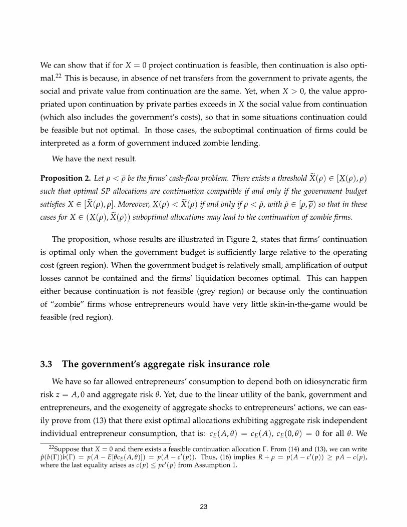
Proposition 2. Let ρ < ρ be the firms’ cash-flow problem. There exists a threshold X(ρ) ∈ [X(ρ), ρ)

such that optimal SP allocations are continuation compatible if and only if the government budget

satisfies X ∈ [X(ρ), ρ]. Moreover, X(ρ) < X(ρ) if and only if ρ < ρ, with ρ ∈ [ρ, ρ) so that in these

cases for X ∈ (X(ρ), X(ρ)) suboptimal allocations may lead to the continuation of zombie firms.

The proposition, whose results are illustrated in Figure 2, states that firms’ continuation

is optimal only when the government budget is sufficiently large relative to the operating

cost (green region). When the government budget is relatively small, amplification of output

losses cannot be contained and the firms’ liquidation becomes optimal. This can happen

either because continuation is not feasible (grey region) or because only the continuation

of “zombie” firms whose entrepreneurs would have very little skin-in-the-game would be

feasible (red region).

3.3 The government’s aggregate risk insurance role

We have so far allowed entrepreneurs’ consumption to depend both on idiosyncratic firm

risk z = A, 0 and aggregate risk θ. Yet, due to the linear utility of the bank, government and

entrepreneurs, and the exogeneity of aggregate shocks to entrepreneurs’ actions, we can eas-

ily prove from (13) that there exist optimal allocations exhibiting aggregate risk independent

individual entrepreneur consumption, that is: cE(A, θ) = cE(A), cE(0, θ) = 0 for all θ. We

22Suppose that X = 0 and there exists a feasible continuation allocation Γ. From (14) and (13), we can writep(b(Γ))b(Γ) = p(A − E[θcE(A, θ)]) = p(A − c′(p)). Thus, (16) implies R + ρ = p(A − c′(p)) ≥ pA − c(p),where the last equality arises as c(p) ≤ pc′(p) from Assumption 1.

23

Figure 2: Optimality of firms’ continuation given operating cost and government budget

Notes: The figure exhibits the region of optimality of firms’ continuation for given ρ and X. In the region labeled“Zombie lending” firms’ continuation is feasible but not optimal. The value of the fixed exogenous parameterscoincides with those in Figure 1 (except for ρ which is a variable in this figure).

focus in the rest of the section on this restricted set of SP allocations and show the importance

of the provision of aggregate risk insurance by the government. Typical contracts between

banks and firms are only contingent on firms’ idiosyncratic outcomes and not on aggregate

variables. Therefore, these results motivate the government tools presented in Section 4 for

the decentralized implementation of optimal allocations, and allow to understand why other

government policies discussed in Section 5 are suboptimal.

Consider an optimal continuation compatible SP allocation with θ-independent entrepreneur

consumption. Each entrepreneur’s consumption can be described by the pay-off b allocated

to outsiders upon his firm’s success. Since d0 + dL = cD, we can write from (6) the expected

and worst aggregate shock contingent overall consumption by depositors and the bank as:

d0 + dL + E[cB(θ)] = pb + E[τ(θ)], (18)

d0 + dL + cB(θ) = θpb + τ(θ). (19)

The LHS in these expressions highlights that the consumption allocated to depositors is

constant, while the RHS shows that the firms’ project value allocated to outsiders under the

worst aggregate shock (θpb) gets reduced relative to its expected value (pb). Such fall must

be accommodated by the bank and/or the government. In fact, subtracting (19) from (18) we

24

have the following aggregate risk insurance accounting identity:

(1− θ)pb︸ ︷︷ ︸Required agg. risk insurance

= E[cB(θ)]− cB(θ)︸ ︷︷ ︸Bank provision agg. risk ins.

+ τ(θ)− E[τ(θ)]︸ ︷︷ ︸Gov. provision agg. risk ins.

. (20)

The LHS of this expression is the reduction of the firms’ value allocated to outsiders under

the worst shock relative to its expected value, which can be interpreted as the aggregate risk

insurance necessary to make savers’ consumption riskless. The RHS includes the sum of

the reduction in the consumption of the bank under the worst shock relative to its expected

consumption and the increase in the government transfers under the worst shock relative

to its expected value. Those variations can be interpreted (if positive) as the aggregate risk

insurance provided by the bank and the government, respectively.

Using that dL + τL = ρ and that (8) - (9) are binding, we have from (18) that

(1− θ)pb︸ ︷︷ ︸Required agg. risk insurance

= (1− θ)(R + ρ− X), (21)

which expresses the required aggregate risk insurance as a fraction 1− θ of the overall value

required for firms’ continuation (R + ρ) minus the government expected disbursement (X).

Also, using cB(θ) ≥ 0, we have that:

E[cB(θ)]− cB(θ)︸ ︷︷ ︸Bank provision agg. risk ins.

≤ R− d0 = (1− θ)R, (22)

which states that an upper bound to the aggregate risk insurance provided by the bank is a

fraction 1− θ of the value that legacy investors must obtain.

The next result follows.

Lemma 2. Let Γ be an optimal SP allocations with aggregate risk independent individual entrepreneur

consumption. The government’s aggregate risk insurance satisfies:

τ(θ)− E[τ(θ)] ≥ (1− θ) (ρ− X) . (23)

The lemma provides a lower bound on the aggregate risk insurance provided by the gov-

ernment disbursements in optimal allocations with θ-independent entrepreneur consump-

tion. The lower bound is strictly positive when the government’s budget is not enough to

cover entirely operating costs (X < ρ). The intuition is that the maximum aggregate risk

insurance the bank can provide allows only to make legacy deposits riskless (which, re-

call, were riskless in the no lockdown economy), but additional aggregate risk insurance is

25

needed in order to make the new deposits riskless. Such additional insurance must be pro-

vided by the government. Notice also from (23) that a government with a low budget must

compensate its inability to directly finance the firms’ operating cost with a higher provision

of aggregate risk insurance in the economy.

Finally, what happens if the government does not provide sufficient aggregate risk in-

surance, that is, if τ(θ) − E[τ(θ)] < (1 − θ) (ρ− X)? Notice that, conditional on firms’

continuation, sufficient aggregate risk insurance must be provided to ensure the full repay-

ment of deposits under bad aggregate shocks. If the government does not provide sufficient

insurance, then, inverting the steps taken above, one can prove that the aggregate risk in-

surance provided by the bank should increase, that is: E[cB(θ)]− cB(θ) > R− d0. But then

E[cB(θ)] > R− d0, that is, the SP finds increasing bank value as the only way to create the

necessary aggregate risk insurance in the economy. From (18), this requires an increase of

the firms’ value allocated to outsiders, reducing entrepreneurs’ effort and social welfare.

4 Implementation with decentralized government policiesIn this Section, we focus on the decentralized implementation of SP optimal allocations.

Recall from the model set-up that the bank provides standard loan financing to the firms

whose repayment is contingent on firms’ idiosyncratic risk. As a result, entrepreneurs’ con-

sumption is aggregate risk insensitive, and from Lemma 2 government policies must provide

sufficient aggregate risk insurance. With this background motivation, we consider a govern-

ment that makes transfers to firms and provides aggregate risk insurance in the economy by

granting fairly priced guarantees on the bank’s deposits.

4.1 Government support policies and competitive equilibrium

A government support policy is described by a pair (τL, κ) consisting of a government

transfer to each firm of τL ≤ X units of funds at t = 0, and a fairly priced government

guarantee on bank deposits described by an aggregate shock parameter κ ∈ [θ, 1] such that

the government insures the repayment of deposits at t = 1 for aggregate shocks θ ∈ [θ, κ],

and requires fair compensation to the bank for aggregate shocks θ > κ.23 We say that a higher

23Since E[θ] = 1, for any guarantee κ ≤ E[θ] = 1 the bank has a sufficient residual claim contingent onshocks θ > κ to reimburse the government for the deposit insurance provided for shocks θ ≤ κ. See AppendixA.2 for a formal description of the contingent transfers τ(θ) associated with a fairly priced guarantee κ ∈ [θ, 1].

26

κ corresponds to a larger deposit guarantee as it allows the bank to enjoy deposit insurance

for a larger set of aggregate shocks. For the sake of expositional simplicity we assume that

government makes the transfer τL to each firm conditional on the firm’s continuation, so that

the expected cost for the government of the policy (τL, κ) is τL if there is firms’ continuation,

and zero otherwise.24

Recall that Assumption 3 implies that R < b0, so that entrepreneurs do not obtain any

value from their firms in case of liquidation and always attempt to obtain financing for their

operating cost. For a support policy (τL, κ), firms need ρ − τL ≥ 0 units of bank funding

at t = 0. If the bank provides such financing in exchange of a promised repayment bL ≥ 0

at t = 1, then firms continue and the new debt promise bL adds to the existing one b0, so

that from (3) the firms’ risk choice increases, p (b0 + bL) ≤ p (b0) = p0. The bank must issue

ρ− τL units of new deposits to finance lending to firms.

The promise bL for the residual financing is feasible if:

• The bank deposits are safe given the guarantee:

d0 + ρ− τL ≤ κ p (b0 + bL) (b0 + bL) . (24)

The LHS of the inequality above captures the bank’s promise to old and new depositors.

The RHS captures that the government’s deposit insurance makes deposits safe for

aggregate shocks θ ≤ κ, allowing safe deposit issuance up to a fraction κ of the expected

value of the bank’s debt portfolio. The guarantee hence relaxes the maximum leverage

constraint imposed by savers.

• The bank finds optimal to grant the new financing rather than liquidating the firms:

Π(bL) ≥ R− d0, (25)

where Π(bL) denotes the bank’s expected profits when new lending is granted and the

24If the transfer were not conditional on the firm’s continuation, the entrepreneur could find optimal to let itsproject be liquidated by the bank and consume the government transfer τL. Notice that Assumption 4 impliesthat when τL is sufficiently close to ρ, the entrepreneur would find optimal to use the government transfer topartially pay the operating cost but not necessarilly so otherwise. It is possible to prove that such potentialopportunistic behaviour by the entrepreneur does not arise under the decentralized implementation of optimalSP allocations described in this section when the SP optimal allocations are continuation compatible, that is,when X ∈

[X(ρ), ρ

]where X(ρ) is defined in Proposition 2. The reason is that, when SP optimal allocations

are continuation compatible, the government’s expected intervention cost is more than offset by an increase inentrepreneurs’ expected consumption.

27

RHS is the bank’s payoff in case of firms’ liquidation. Since the government guarantee

is fairly priced, we have that:

Π(bL) = p (b0 + bL) (b0 + bL)− d0 − ρ + τL. (26)

Finally, whenever a feasible promise bL for the residual financing exists given a policy (τL, κ) ,

we define the competitive promise b∗L (τL, κ) as the feasible promise with lowest bL. Notice that

such promise maximizes the firms’ profits. It can be proved that the competitive promise

arises as the outcome of Bertrand competition in the lending market between the bank and a

potential new bank entrant that can also benefit from the government guarantee on deposits.

4.2 The competitive bank residual financing

Consider a government intervention (τL, κ) with τL ≤ X and κ ∈ [θ, 1]. Notice τL = 0

and κ = θ corresponds to no intervention. We next analyze the outcome of the competitive

financing of firms’ residual funding needs. In order to gain more intuition on how the bank

intermediates between savers and firms, we can use Assumption 5 to rewrite the bank’s

maximum leverage constraint in (24) as:

ρ− τL ≤ θ [ p (b0 + bL) (b0 + bL)− p (b0) b0] + (κ − θ) p (b0 + bL) (b0 + bL) . (27)

The inequality above can be interpreted as the bank’s lending constraint. The LHS captures

the new deposits the bank has to issue to finance firms. The two terms in RHS exhibit how

the bank can fund those deposits. The first one captures the additional deposits the bank

can issue from its new lending if its leverage remained fixed at θ. From Lemma 1, this term

is increasing in bL for bL ∈ [0, bmax − b0] so that the bank has some capability to issue new

deposits even in absence of deposit guarantees. The second term, which is increasing in the

size κ of the deposit guarantee, captures the additional deposit issuance capability due to

the increase in leverage allowed by the guarantee. For given κ, the RHS has a maximum

at bL = bmax − b0, so the bank has a maximum capacity to provide deposits. Hence, when

ρ− τL is high continuation might only be feasible for high guarantee size κ.

Suppose that there exists a feasible promise bL. Since provided bL ∈ [0, bmax − b0] the

constraints (24) and (25) get relaxed as bL increases, it is easy to prove that the competitive

promise b∗L makes at least of one of the constraints binding.

Suppose for the time being that the bank’s leverage constraint in (24) is binding. We have

28

that the bank’s expected profits in (26) can be rewritten as the following function of (τL, κ):

Π(τL, κ) = (d0 + ρ− τL)1− κ

κ. (28)

The expression shows that the bank’s profits amount to the product of its deposits (d0 +

ρ− τL) and a term that captures the rents the bank obtains per unit of deposits ((1− κ)/κ).

For given guarantee κ, the bank’s profits are increasing in the funding ρ − τL demanded

by firms because the maximum leverage constraint faced by the bank prevents competition

from reducing to zero the lending rents the bank obtains. In addition, the rents per unit

of deposit obtained by the bank are decreasing in the deposit guarantee κ. The intuition is

that an increase in the deposit guarantee, relaxes the bank’s funding constraint allowing it

to expand its supply of lending (equation (27)). As a result, the competitive bank reduces

the promise b∗L, which leads to a reduction in its profits. Hence, the government provision

of aggregate risk insurance through fairly priced deposit guarantees κ allows to reduce the

rents the bank obtains from providing new lending to firms.

Notice from (28) that for κ sufficiently close to one, the profits of a bank that were to

maximize its leverage given the deposit guarantees would approach to zero, in which case

its participation constraint (25) would not be satisfied. Hence, there is a maximum level of

guarantees κ above which the competitive b∗L makes the participation constraint (25) binding

while the maximum leverage constraint (24) is slack. Further increases in the deposit guar-

antee do not lead neither to increases in bank leverage nor to reductions in b∗L. Thus, there is

a limit to the support that can be given to firms by granting deposit guarantees.

Building on these intuitions we obtain the next result.

Proposition 3. Let X(ρ) < ρ be the continuation feasibility threshold defined in Proposition 1.

There exist two increasing functions κ(`), κ(`) ∈ [θ, 1) defined in the interval ` ∈ [0, ρ − X(ρ)],

with κ(`) < κ(`) for 0 < ` < ρ− X(ρ) and κ(`) = θ for ` in a neighborhood of zero, such that

interventions (τL, κ) lay in one of these regions:

• If τL < X(ρ), or τL ≥ X(ρ) and κ < κ(ρ− τL): Firms do not obtain bank lending and are

liquidated.

• If τL ≥ X(ρ) and κ ∈ [κ(ρ − τL), κ(ρ − τL)): Firms obtain bank lending and the bank’s

leverage constraint is binding. The competitive promise b∗L(τL, κ) and the bank’s profits Π(τL, κ)

are strictly decreasing in τL and κ.

29

• If τL ≥ X(ρ) and κ > κ(ρ− τL): Firms obtain bank lending and the bank’s leverage constraint

is not binding. The competitive promise b∗L(τL, κ) is strictly decreasing in τL and constant in κ,

and Π(τL, κ) = R− d0.

The proposition describes how government support policies affect firms’ access to financ-

ing and the bank’s profits. The results are illustrated in Figure 3, in which firms obtain

financing only in the colored regions. For a given deposit guarantee, the financing that firms

can get is limited by either the bank’s capability to raise new deposits (leverage constraint

(24), LC) or by its willingness to provide lending (participation constraint (25), PC). The func-

tion κ(ρ− τL) (orange line) represents the minimum guarantee that allows the bank to obtain

the residual financing needs given the limit imposed by the bank’s LC. The function κ(ρ− τL)

(green dashed line) instead represents the maximum deposit guarantee for which a bank that

chooses maximum leverage satisfies its PC. Hence, in the purple region, the deposit guaran-

tee is large enough to afford banks’ sufficient lending capability, but not too large so that the

bank chooses maximum leverage and still obtains some profits relative to liquidation. As the

guarantee κ increases in this purple region, the associated competitive promise b∗L and bank

profits go down. The government is in fact providing larger aggregate risk insurance, which

reduces the equilibrium loss absorption capacity the bank must have, and hence the value

of its equity. If the guarantee increases further, the economy enters into the green region, in

which the bank’s LC becomes slack. The reason is that if the bank were to choose maximum

leverage, the financing to firms would be so cheap that the bank’s PC would not be satisfied.

An increase in the guarantee κ in this green region, has no effect on bank’s leverage choice

nor on b∗L.

4.3 Optimality of the government toolkit and optimal policy mix

We now show that a government with support policies (τL, κ) with τL ≤ X, κ ∈ [θ, 1] is

able to achieve SP optimal allocations interventions and characterize optimal policies (τL, κ)

as a function of the government’s budget X.

Consider a government budget satisfying X ≥ X(ρ), so that from Proposition 2 optimal

SP allocations induce continuation, and define the support policy (τL, κ) with τL = X and

κ ≥ κ(ρ−X), where κ(.) is defined in Proposition 3. The policy (τL, κ) is optimal as it satisfies

the conditions in Proposition 1. In fact, taking into account that X(ρ) ≥ X(ρ), Proposition 3

30

Figure 3: Bank’s leverage and participation constraints for given intervention

Notes: The figure exhibits the three regions described in Proposition 3. LC refers to the leverage constraint (24)and PC to the participation constraint (25). Outside the colored areas continuation is not feasible. The level `defines the maximum new lending (new deposits) feasible, defined by: Π(bL = bmax − b0, `) = p (bmax) bmax −d0 − ` = R− d0. Notice that ` = ρ− X(ρ) when X(ρ) > 0. Parameter values coincide with those in Figure 1(except for ρ which is a variable in this figure).

implies that (τL, κ) induces continuation and makes the bank’s participation constraint bind-

ing. The remaining three optimality conditions in Proposition 1 are also trivially met. First,

in case of project failure, the entrepreneur defaults on the loan and its consumption equals

zero, that is: cE(θ, 0) = 0. Second, since savers provide funding to banks in a competitive

market, their participation constraint is binding. Third, the government’s budget constraint

is binding because τL = X.

The next result follows.

Proposition 4. Let X(ρ) and κ(l) the objects defined in Proposition 2 and 3, respectively. If X ∈[X(ρ), ρ], a government support policy (τL, κ) induces an optimal SP allocation if and only if τL = X

and κ ≥ κ(ρ− X). Such support policies induce firms’ continuation, bank’s leverage equal to κ(ρ−X) and government provision of aggregate risk insurance equal to (1− θ)(ρ− X). If 0 ≤ X < X(ρ)

then no government support (τL = 0, κ = θ) induces liquidation and optimal SP allocations.

The proposition states that the policy toolkit (τL, κ) allows to implement optimal SP allo-

cations through the competitive bank intermediation of funds from savers to firms. Indeed,

31

the government can use its entire (expected) budget to grant transfers to firms and com-

bine them with sufficiently large fairly priced guarantees to bank deposits. The guarantees

provide aggregate risk insurance in the economy, allowing the competitive bank to increase

its leverage to provide cheap financing to the firms. When the guarantee is large enough

(κ ≥ κ(ρ − X)), the bank does not obtain any rents from new lending as the loss absorp-

tion capacity provided by its equity is not any more scarce, and entrepreneurs’ effort and

aggregate welfare are maximized.25 The support policy (τL, κ) implements an optimal al-

location. Notice that the proposition states that the government’s provision of aggregate

risk insurance, which amounts to the cost of deposit insurance under the worst aggregate

shock, is equal to (1− θ)(ρ−X). From Lemma 2, the government is providing the minimum

aggregate risk insurance necessary for optimality.

Figure 4 further illustrates the importance of the provision of aggregate risk insurance by

comparing the outcome under an optimal (τL = X, κ ≥ κ(ρ − X)) policy with that under

a policy that relies solely on transfers to firms (τL = X, κ = θ) for different values of the

government’s budget X. The first difference in the outcome induced by the two policies

is that for low X, the firms’ continuation is only feasible when the policy includes deposit

guarantees.26 For larger values of X, the two policy toolkits allow the firms’ continuation but

the competitive promise b∗L for the residual financing ρ−X demanded by firms is lower when

deposit guarantees are used (Panel 4a). This is because deposit guarantees provide aggregate

risk insurance that allows the bank to increase its leverage (Panel 4b). When only transfers

are used, the bank must provide all the aggregate risk insurance to finance the new deposits,

leading to higher bank profits relative to those in the no-lockdown economy, which coincide

with those under optimal policies with deposit guarantees (Panel 4c). Finally, the bank rents,

induced when only transfers are used, make lending expensive and increase the firms’ value

allocated to outsiders, aggravating moral hazard problems and amplifying initial output

losses (Panel 4d). Notice that as the government budget increases further, the differences

between the outcomes under the two policy interventions get narrowed. The reason is that

25Notice instead that any policy in which κ < κ(ρ − X), represented by the purple region in Figure 3,generates rents to the bank, which makes the competitive b∗L inefficiently high and induces a suboptimal effortchoice and welfare.

26This happens when ρ ∈ (θρ, ρ) , so the operating cost is high enough such that κ(ρ) > θ, but still X(ρ) = 0.

32

as the amount of new safe debt raised by the bank is reduced, the need of the aggregate risk

insurance provided by the government through debt guarantees also diminishes.

5 Government policies with other guaranteesWe have seen in the previous Section that transfers to firms and fairly priced guarantees

on bank deposits constitute an optimal policy toolkit. Yet, while the former policy has been

used in many jurisdictions in response to the Covid-19 crisis, the latter policy has not. Gov-

ernments have instead relied on the introduction of guarantees in bank loans to firms. Also,

most supervisory authorities have released capital buffers, whose effect in the context of our

model would be equivalent to the introduction bank deposit guarantees that do not have to

be reimbursed upon good shocks.

In this section, we analyze the capability to achieve optimal allocations under two alter-

native government intervention toolkits in which fairly priced bank deposit guarantees are

substituted with non-priced bank deposit guarantees and bank loan guarantees, respectively.

We find that, when the government budget is low, these policies provide a suboptimal sub-

stitute to fairly priced deposit guarantees because they do not provide sufficient aggregate

risk insurance.

Alternative toolkit 1: Transfers and non-priced bank debt guarantees

As first alternative intervention toolkit, we consider (τL, κfree) policies consisting of a

transfer τL ≥ 0 to firms and a bank debt guarantee described by the variable κFree ≥ θ with

the only difference that the government grants it for free. Notice that the bank’s maximum

leverage constraint under this intervention remains as that in (24), while the fact that the

debt guarantee is not repaid by the bank would be captured in its expression for profits

that would include an additional term to those in (26) capturing the value of the deposit

insurance.27

For a policy (τL, κFree) with τL < ρ, κFree > θ that allows firms’ continuation, we denote b∗Lthe competitive promise in exchange for the bank’s residual financing ρ− τL. If the bank’s

27Appendix A.2 provides a more complete formal description of the two alternative policy toolkits discussedin this section.

33

(a) Bank new loan promise: b∗L(b) Bank debt to assets ratio: d0+ρ−τL

p(b0+b∗L)(b0+b∗L)

(c) Bank Profits: Π(b∗L) (d) Welfare relative to no-lockdown: Y(b∗L)−Y0

Figure 4: Equilibrium under optimal policies and only transfers for given government bud-get.

Notes: The figure exhibits the competitive new loan promise, b∗L , bank debt to assets ratio,d0+ρ−τL

p(b0+b∗L)(b0+b∗L),

bank profits, Π(b∗L), and welfare difference relative to the no-lockdown benchmark, Y(b∗L) − Y0, under anoptimal policy (τL = X, κ ≥ κ(ρ − X)) and an only-transfers policy (τL = X, κ = θ) as a function of thegovernment budget X. The value of the exogenous parameters coincides with that in Figure 1.

34

maximum leverage constraint is binding for the promise b∗L, the government’s θ-contingent

transfer to the bank at t = 1 to pay the debt guarantee is

τ(θ) = (d0 + ρ− τL − θ p(b0 + b∗L)(b0 + b∗L))+ = (d0 + ρ− τL)

(κfree − θ)+

κfree, (29)

where the second equality uses that (24) is binding. The transfer τ(θ) is decreasing in θ and

equals zero for θ > κfree. Thus, the government provision of aggregate risk insurance is:

τ(θ)− E[τ(θ)] =(

κfree − θ

E[(κfree − θ)+]− 1)

E[τ(θ)] > 0. (30)

The expression shows that the aggregate risk insurance provided by the government is

proportional to its expected expenditure, E[τ(θ)], which in turn is limited by its budget,

E[τ(θ)] ≤ X. While non-priced debt guarantees provide some insurance and will allow to

improve welfare relative to the sole use of transfers, when the government budget X is suffi-

ciently small relative to the operating cost ρ, the government will not be able to provide the

minimum aggregate risk insurance given in (23) necessary to achieve optimality. The toolkit

(τL, κfree) is hence, in general, suboptimal.28

Alternative toolkit 2: Transfers and bank loan guarantees

As second alternative intervention toolkit, we consider (τL, γ) policies consisting of a

transfer τL ≥ 0 to firms and a guarantee on the new bank lending to firms described by the

fraction γ ∈ [0, 1] of the new lending promise bL that the government pays to the bank in

case of a firm’s failure.

For a policy (τL, γ), the analogous constraint to (24) establishing the maximum bank

leverage constraint imposed by savers is

d0 + ρ− τL ≤ θ p (b0 + bL) (b0 + bL) + (1− θ p (b0 + bL)) γbL. (31)

The second term in the RHS of this expression captures that under the shock θ a fraction

1 − θ p(b0 + bL) of the bank debt portfolio defaults and the bank obtains the government

guaranteed amount γbL. Loan guarantees thus relax the bank’s leverage constraint, allowing

the bank to provide cheaper financing to firms (lower bL), which increases welfare.

For a policy (τL, γ) with τL < ρ, γ > 0 that allows firms’ continuation, we can denote b∗Lthe new lending promise. The government’s θ-contingent transfer to the bank at t = 1 to

28Yet, it is possible to prove that when X is close to ρ, the government can provide enough insurance and(τL, κfree) policies can achieve optimal allocations.

35

repay loan guarantees is

τ(θ) = (1− θ p(b0 + b∗L)) γb∗L, (32)

which is a decreasing function in θ and strictly positive for all θ. The government provision

of aggregate risk insurance through loan guarantees is:

τ(θ)− E[τ(θ)] =(1− θ) p(b0 + b∗L)

1− p(b0 + b∗L)E[τ(θ)] > 0. (33)

As in our discussion above, the government provision of aggregate risk insurance through

loan guarantees is limited by its budget, so it will not provide enough insurance when it has

a low budget. The toolkit (τL, γ) is hence, in general, also suboptimal.29

Comparison of the policy toolkits. Figure 5 compares, for different government budgets, the

outcome under the optimal use of the three intervention toolkits: i) direct transfers and fairly

priced deposit guarantees (τL, κ), in orange solid-line, ii) direct transfers and non-priced

deposit guarantees (τL, κfree), in purple dashed-line, and iii) direct transfers and banks loan

guarantees (τL, γ), in black dotted-line. Notice that the plot of the dash and dotted-lines

does not start at a zero government budget because, for the parameters in the numerical

illustration, firms’ continuation is not optimal under the alternative intervention toolkits.

Panel 5a exhibits the share of the government budget that is used for direct transfers un-

der the optimal policy mix in each intervention toolkit. By construction, fairly priced deposit

guarantees have a zero expected cost for the government, which can use its entire budget to

grant transfers. In contrast, the government uses some of its budget for the provision of the

two other types of guarantees. The figure shows in fact that when the government’s bud-

get is low it is optimal to allocate the budget entirely to the provision of guarantees, while

transfers are also used when the budget is larger. The reason is that, from Lemma 2, when

the government has a low budget the economy has large needs of aggregate risk insurance,

which is provided by the guarantees.

Panel 5b shows the aggregate risk insurance provided under each intervention. Recall

that the insurance provided under optimal (τL, κ) interventions equals, from Lemma 2 and

Proposition 4, the minimum insurance provision required to achieve optimal allocations. In

contrast, the insurance provided by optimal (τL, κfree) and (τL, γ) interventions is limited by

29Again, it is possible to prove that when X is close to ρ, the government can provide enough aggregate riskinsurance insurance and (τL, γ) policies can achieve optimal allocations.

36

the government’s budget. So, when it is low, they provide less insurance than necessary to

achieve optimal allocations. As the budget increases, the insurance provided by these poli-

cies increases, while the minimum insurance provision required for optimality decreases.

For large enough government budget, the alternative toolkits provide sufficient insurance

to achieve optimal allocations. Finally, notice that for low budget, the insurance provided

under optimal (τL, κfree) interventions is larger than under optimal (τL, γ) interventions. The

reason is that guarantees on bank deposits only give rise to disbursements to satisfy a short-

fall between the payoff of the bank’s assets and its overall amount of deposits, so that by

definition they lead to the minimum disbursement that ensures the safety of the deposits.

Loan guarantees are instead a less targeted way to provide aggregate risk insurance since,

due to the presence of idiosyncratic firm risk, they imply a government disbursement even

when aggregate shocks are positive and the bank makes profits at the final date. So, part of

the budget is used to transfer resources to the bank upon good shocks, which “wastes” some

of the scarce government budget at expense of transfers during bad shocks.

Panels 5c and 5d illustrate how aggregate risk insurance provision affects bank profits and

social welfare, respectively. When the alternative intervention toolkits do not provide suffi-

cient aggregate risk insurance by the government (that is, for low budget X), the bank must

complement the shortfall through the creation of additional loss absorption capacity out of its

portfolio of debt to firms. This requires an increase in the equilibrium promise of firms to the

bank b∗L, so that the the safe collateral value of the bank assets θ p(b0 + b∗L)(b0 + b∗L) increases

enough to grant the bank additional capability to repay deposits under all contingencies.

Thus, the scarcity of loss absorption in the economy to back intermediation from savers to

firms, increases firms’ borrowing cost, inducing some bank profits and amplifying welfare

losses due to the aggravation of firms’ moral hazard. Conversely, when the alternative inter-

vention toolkits provide sufficient aggregate risk insurance (that is, for large budget), they

minimize bank profits and maximize welfare.

Two final comments on the relationship between the optimal policy mix (Panel 5a), pro-

vision of aggregate risk insurance (Panel 5b), bank profits (Panel 5c), and welfare (Panel 5d)

under the alternative toolkits are worth. First, it is optimal to make use of direct transfers

to firms under the alternative toolkits only when sufficient aggregate risk insurance has al-

ready been granted through guarantees, so that bank profits are minimum and welfare is

37

maximum. The reason is that, once the intervention provides sufficient aggregate risk in-

surance, the financial frictions imposed by savers demanding safety are not longer binding,

and additional (bank debt or loan) guarantees do not induce the bank to increase its lever-

age further and pass on cheaper financing to firms. As the reduction of the firms funding

cost through guarantees loses traction, a government with a large budget must thus com-

bine them with some direct transfers to firms. Second, for a low budget government, the

larger capability to provide aggregate risk insurance through (τL, κfree) interventions relative

to (τL, γ) interventions translates into lower bank profits and higher welfare. In presence of

political economy constraints that prevent the government to intervene through policies that

include some form of reimbursement upon future good shocks, it is thus preferable to rely

on bank debt guarantees rather than loan guarantees.

6 Funding of aggregate risk insurance provisionProposition 4 shows that a government with expected budget X ≥ 0 can implement

optimal SP allocations with combinations of transfers τL = X to firms at t = 0 and sufficiently

large fairly priced guarantees on bank deposits characterized by a parameter κ ≥ κ(ρ− X).

The government provides aggregate risk insurance in the economy at zero expected cost

through guarantees that imply transfers τ∗(θ) > 0 to the bank at t = 1 following bad shocks,

and reimbursements τ∗(θ) < 0 from the bank at t = 1 following good shocks, that net out

in expectation, E[τ∗(θ)] = 0. If we denote b∗L the associated competitive promise on the new

bank loan for the provision of ρ − X units of funds to the firms and p∗ = p(b0 + b∗L) the

associated risk choice of the firms, we have that when the bank defaults on the deposits, the

transfer τ∗(θ) > 0 the government has to do to repay deposits amounts to:

τ∗(θ) = d0 + ρ− X− θp∗(b0 + b∗L). (34)

The RHS in the expression above is in fact the difference between the overall amount of

deposits in the economy and the payoff of the bank portfolio of loans to firms.30 As can be

seen from the aggregate resource constraint in (6), transfers from the government increase

the overall consumption of savers, the bank and entrepreneurs at the final date. Our stylized

model aims at capturing in a reduced form manner a government that has some capability to

30See Appendix A.2 for the expression of the reimbursements τ∗(θ) < 0 to the government associated withthe fairly priced guarantee κ ∈ [θ, 1] for shocks θ ≥ κ.

38

(a) Share of budget used for direct transfers: τL/X (b) Aggregate risk insurance: τ(θ)− E[τ(θ)]

(c) Bank profits: Π (d) Welfare relative to no-lockdown: Y−Y0

Figure 5: Comparison of intervention toolkits

Notes. Share of budget used for direct transfers τL/X, provision of aggregate risk insurance τ(θ) − E[τ(θ)],bank profits Π, and welfare difference relative to the no-lockdown benchmark Y−Y0, under an optimal policy(τL = X, κ = κ(ρ − X)) (solid orange line), the optimal mix of transfers with non-priced deposit guarantees(τL, κfree) (dashed purple line), and the optimal mix of transfers with loan guarantees (τL, γ) (black dotted line)as a function of government budget X. Parameter values coincide with those in Figure 1.

39

obtain external resources from the taxation of some unmodeled agents or by issuing debt that

is repaid from taxation at some unmodeled future date. Yet, under optimal interventions the

government needs to obtain resources precisely upon bad aggregate shocks, which might

raise concerns on whether those policies would be implementable in practice.

We analyze in this section whether the government can finance the issuance of those

guarantees on bank deposits internally, through taxation and redistribution of the resources

of the agents in the economy at t = 1. There are three agents that could be potentially taxed:

savers, the bank and entrepreneurs. Savers’ returns on their investments in bank deposits

cannot be taxed because they are infinitely risk-averse and that is in the first place the reason

why the economy needs aggregate risk insurance. There are no resources the government

can tax to the bank when the bank defaults in its own debt. These leaves as only agents

to tax at t = 1 the entrepreneurs whose firms succeed. In fact, these firms generate profits

amounting to A− (b0 + b∗L) .

Is it possible to finance the deposit guarantee through taxation and redistribution between

these agents and the bank? Suppose that when τ∗(θ) > 0 the government, instead of raising

external resources to repay deposits in full, imposes a tax t(θ) > 0 to the measure θp∗ of

successful firms and uses it to repay deposits. The size of the tax on each entrepreneur is

determined by the following overall taxation proceeds constraint:

τ∗(θ) = θp∗t(θ). (35)

And conversely, when τ∗(θ) < 0 the government distributes the bank’s reimbursement on the

deposit guarantee to successful firms through a transfer t(θ) < 0 to each of the measure θp∗of

them, where t(θ) is also determined by (35). Notice that the consumption of a successful

entrepreneur becomes cE(A, θ) = A− b0 + b∗L − t(θ), and it is not any more θ−independent.

This alternative financing would work provided two conditions are met: the competitive loan

promise and the firms’ risk choice do not change as a result of the tax; and the successful

entrepreneurs have collectively sufficient resources that can be taxed. We analyze next if the

two conditions can be jointly met.

First, who provides the guarantee does not affect the competitive bank loan promise nor

the firms’ risk choice.31 In fact, we have from (24) and (25) that the competitive bank loan

31More precisely, in this paragraph we analyze whether this condition is satisfied provided the secondcondition, discussed in the next paragraph, is also satisfied.

40

pricing given a guarantee κ does not depend on whether the government or the firms are the

counterpart of the associated transactions to the extent that being the guarantee counterpart

does not affect the firm’s risk choice function p(b). That is in fact the case because the optimal

risk-choice of a firm with overall debt b under taxation upon success t(θ) satisfies :

p = arg maxp′

E

θp′ (A− b− t(θ))− c(p′)⇐⇒ (36)

c′ (p) = A− b− E[θt(θ)] = A− b0 − b∗L ⇐⇒ p = p (b) (37)

where we have used that E[θt(θ)] = E[τ∗(θ)]/p∗ = 0, which results from the construction of

the tax t(θ) and (4). While the tax to entrepreneurs upon success in bad shocks reduces their

incentives to exert effort, the transfers they get upon success in good shocks increase effort

incentives and these effects offset each other.

Second, when τ∗(θ) > 0, the successful entrepreneurs have collectively sufficient re-

sources that can be taxed.32 The taxation on each of the measure θp∗ of successful en-

trepreneurs is upper bounded by their profits, A− b0 − b∗L, so that these agents have collec-

tively enough resources if and only if

τ(θ) ≤ θp∗ (A− b0 − b∗L) .

From (34), the LHS in the expression above is decreasing in θ, while its RHS is increasing.

The condition is thus most stringent under the worst shock θ, for which using (34) it becomes:

d0 + ρ− X ≤ θp∗A. (38)

The expression states that the deposit guarantee can be paid through taxation of successful

entrepreneurs when the overall amount of deposits in the economy (LHS in the expression

above) does not exceed the overall payoff of the firms given the worst shock (RHS in the

expression above). The inequality can in fact be interpreted as the overall internal safe collateral

constraint of the economy. When it is satisfied, the government can finance internally the

provision of aggregate risk insurance through taxation of entrepreneurs. When it is not,

there is not enough internal safe collateral to back the guarantees on bank deposits, and the

government must rely on external resources.

The next proposition characterizes when internal safe collateral in the economy is suffi-

cient.

32More precisely, in this paragraph we analyze whether this condition is satisfied provided the first condition,discussed in the previous paragraph, is also satisfied. Notice this prevents us from falling into a fallaciouscircular argument.

41

Proposition 5. Let X(ρ) be the object defined in Proposition 2 and let X ∈ [X(ρ), ρ]. There exists a

threshold θ′ > 0 such that the fairly priced deposit insurance associated with an optimal interventions

(τL, κ) can be internally funded through taxation and redistribution to successful entrepreneurs if and

only if θ ≥ θ′.

The proposition states that, if the output destruction under the worst aggregate shock is

not too large, it is possible for the government to finance the fairly priced deposit guarantees

associated with optimal interventions (τL, κ) through taxation of successful entrepreneurs’

profits under bad shocks and redistribution to these agents of deposit insurance fees paid

by the bank under good shocks. This type of procyclical corporate profit taxation removes

the bank’s funding constraint by effectively allowing it to issue deposits not only against

the lowest return of its portfolio of loans to firms, θp∗(b0 + b∗L), but to the entire output of

the economy in that contingency, θp∗A. When the destruction of output in the worst shock

is not too large, the overall internal safe collateral of the economy is sufficient to back the

new issuance of safe deposits implied by the lockdown. In those cases, the government

does not need to inject external resources in the economy but to complete contracts between

the bank and the firms in a way that entrepreneurs with idiosyncratic good shocks make

a transfer to the bank upon bad aggregate shocks that is additional to the loan repayment.

The proposition also implies that when the destruction of output upon the worst shock

is sufficiently large, the financing of aggregate risk insurance under optimal interventions

(τL, κ) necessarily involves the government obtaining external resources upon sufficiently

bad shocks.33 In those cases the procyclical corporate profit taxation described in this section

would nevertheless allow to reduce (but not eliminate), the need of those external resources.

7 ConclusionWe analyze optimal design of interventions of a government with a limited fiscal budget

to support firms facing liquidity needs during a lockdown. The analysis is conducted in a

novel competitive model of financial intermediation with financial frictions at both the firm

and bank level and highlights the amplification of losses through the balance sheets linkages

between firms and banks.

33More generally, it can be proved that when θ < θ′ there is no continuation compatible SP allocation withconstant government transfers τ(θ) at t = 1.

42

Two crucial assumptions drive the results in our model. First, the increase in debt re-

quired by firms to survive the lockdown reduces firms’ equity, creating moral hazard fric-

tions that affect both firms’ output and the return of banks’ loan portfolios. Second, banks

must finance their lending to firms from investors which demand safety. The presence of

both idiosyncratic and aggregate risk gives a role to banks’ equity in addition to firms’ eq-

uity. The need for aggregate risk absorption capacity to intermediate funds restricts lending

supply and leads to equilibrium rents on the scarce banks’ equity, making firm borrowing

more expensive and further amplifying output losses.

Government interventions aimed at limiting output losses are optimal when their design

provides sufficient aggregate risk insurance to bank debt investors. This constitutes a substi-

tute for the loss absorption role of bank equity, which eliminates bank intermediation rents

and reduces borrowing costs and overall firms’ indebtedness. Optimal interventions can be

implemented with a mix of direct grants to firms and fairly priced guarantees on bank debt.

The latter provide aggregate risk insurance in the economy, and are repaid in expectation by

banks upon good shocks. The government can reduce, or even eliminate, the need to issue

public debt upon bad shocks to satisfy the disbursements associated with these guarantees

through the taxation of firms’ profits upon bad shocks and the redistribution to non default-

ing firms of the fees paid by the banks on the guarantees upon good shocks. This procyclical

taxation and redistribution between firms and banks sustains economic activity because it

relaxes banks’ funding cosntraints without aggravating firms’ moral hazard problems.

Finally, some of the common intervention toolkits deployed during the current Covid-

19 crisis are not optimal for governments with a low budget as they provide insufficient

aggregate risk insurance. That is the case in particular when grants to firms are combined

with either non-priced bank debt guarantees or bank loan guarantees. These guarantees

induce larger government disbursements upon bad aggregate shocks, and thus constitute a

form of aggregate risk insurance in the economy. Yet, since they are not reimbursed by the

private sector, they consume part of the government budget that as a result cannot be used

to grant transfers to firms.

43

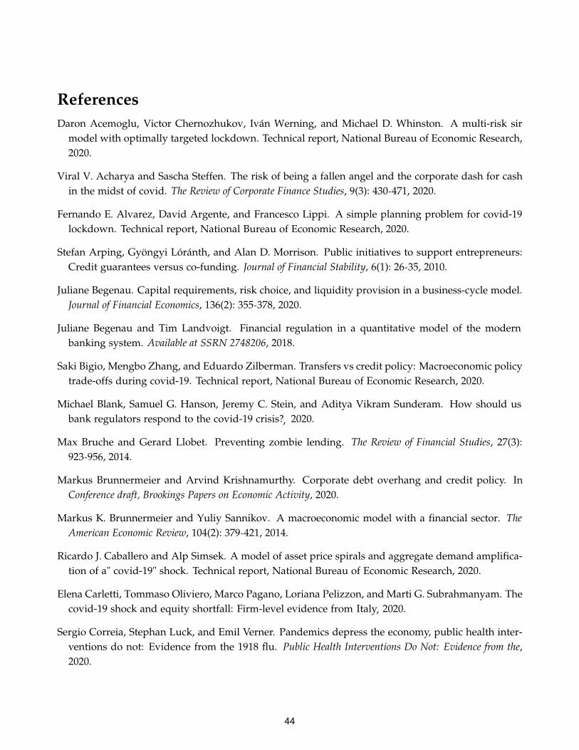
ReferencesDaron Acemoglu, Victor Chernozhukov, Iván Werning, and Michael D. Whinston. A multi-risk sir

model with optimally targeted lockdown. Technical report, National Bureau of Economic Research,2020.

Viral V. Acharya and Sascha Steffen. The risk of being a fallen angel and the corporate dash for cashin the midst of covid. The Review of Corporate Finance Studies, 9(3): 430-471, 2020.

Fernando E. Alvarez, David Argente, and Francesco Lippi. A simple planning problem for covid-19lockdown. Technical report, National Bureau of Economic Research, 2020.

Stefan Arping, Gyöngyi Lóránth, and Alan D. Morrison. Public initiatives to support entrepreneurs:Credit guarantees versus co-funding. Journal of Financial Stability, 6(1): 26-35, 2010.

Juliane Begenau. Capital requirements, risk choice, and liquidity provision in a business-cycle model.Journal of Financial Economics, 136(2): 355-378, 2020.

Juliane Begenau and Tim Landvoigt. Financial regulation in a quantitative model of the modernbanking system. Available at SSRN 2748206, 2018.

Saki Bigio, Mengbo Zhang, and Eduardo Zilberman. Transfers vs credit policy: Macroeconomic policytrade-offs during covid-19. Technical report, National Bureau of Economic Research, 2020.

Michael Blank, Samuel G. Hanson, Jeremy C. Stein, and Aditya Vikram Sunderam. How should usbank regulators respond to the covid-19 crisis? 2020.

Max Bruche and Gerard Llobet. Preventing zombie lending. The Review of Financial Studies, 27(3):923-956, 2014.

Markus Brunnermeier and Arvind Krishnamurthy. Corporate debt overhang and credit policy. InConference draft, Brookings Papers on Economic Activity, 2020.

Markus K. Brunnermeier and Yuliy Sannikov. A macroeconomic model with a financial sector. TheAmerican Economic Review, 104(2): 379-421, 2014.

Ricardo J. Caballero and Alp Simsek. A model of asset price spirals and aggregate demand amplifica-tion of a" covid-19" shock. Technical report, National Bureau of Economic Research, 2020.

Elena Carletti, Tommaso Oliviero, Marco Pagano, Loriana Pelizzon, and Marti G. Subrahmanyam. The

Sergio Correia, Stephan Luck, and Emil Verner. Pandemics depress the economy, public health inter-ventions do not: Evidence from the 1918 flu. Public Health Interventions Do Not: Evidence from the,2020.

44

covid-19 shock and equity shortfall: Firm-level evidence from taly , 2020.

,

I

Martin S. Eichenbaum, Sergio Rebelo, and Mathias Trabandt. The macroeconomics of epidemics.Technical report, National Bureau of Economic Research, 2020.

Vadim Elenev, Tim Landvoigt, and Stijn Van Nieuwerburgh. A macroeconomic model with financiallyconstrained producers and intermediaries. Technical report, National Bureau of Economic Research,2020a.

Vadim Elenev, Tim Landvoigt, and Stijn Van Nieuwerburgh. Can the covid bailouts save the economy?Technical report, National Bureau of Economic Research, 2020b.

Miguel Faria-e Castro. Fiscal policy during a pandemic. FRB St. Louis Working Paper, (2020-006), 2020.

FSB. Covid-19 pandemic: Financial stability impact and policy responses. Financial Stability Board.November, 2020.

Nicola Gennaioli, Andrei Shleifer, and Robert W. Vishny. A model of shadow banking. The Journal ofFinance, 68(4): 1331-1363, 2013.

Mark Gertler and Nobuhiro Kiyotaki. Financial intermediation and credit policy in business cycleanalysis. Handbook of monetary economics, 3(11): 547-599, 2010.

Veronica Guerrieri, Guido Lorenzoni, Ludwig Straub, and Iván Werning. Macroeconomic implicationsof covid-19: Can negative supply shocks cause demand shortages? Technical report, NationalBureau of Economic Research, 2020.

Zhiguo He and Arvind Krishnamurthy. A macroeconomic framework for quantifying systemic risk.Technical report, National Bureau of Economic Research, 2014.

Bengt Holmstrom and Jean Tirole. Financial intermediation, loanable funds, and the real sector. TheQuarterly Journal of economics, pages 663-691, 1997.

Bengt Holmstrom and Jean Tirole. Private and public supply of liquidity. Journal of political Economy,106(1): 1-40, 1998.

IMF. Global financial stability report: Bridge to recovery. International Monetary Fund, Washington, DC.October, 2020.

Callum J. Jones, Thomas Philippon, and Venky Venkateswaran. Optimal mitigation policies in a pan-demic: Social distancing and working from home. Technical report, National Bureau of EconomicResearch, 2020.

Lei Li, Philip E. Strahan, and Song Zhang. Banks as lenders of first resort: Evidence from the covid-19crisis. The Review of Corporate Finance Studies, 9(3): 472-500, 2020.

45

Stewart C. Myers. Determinants of corporate borrowing. Journal of financial economics, 5(2): 147-175,1977.

NAO. Investigation into the bounce back loan scheme. National Audit Office. October, 2020.

Thomas Philippon and Philipp Schnabl. Efficient recapitalization. The Journal of Finance, 68(1): 1-42,2013.

Adriano A. Rampini and S. Viswanathan. Financial intermediary capital. The Review of Economic Studies,86(1): 413-455, 2019.

Rafael Repullo and Javier Suarez. Entrepreneurial moral hazard and bank monitoring: a model of thecredit channel. European Economic Review, 44(10): 1931-1950, 2000.

Anatoli Segura and Javier Suarez. Optimally solving banks’ legacy problems. Technical report, CEPRDiscussion Papers, 2019.

Alonso Villacorta. Business cycles and the balance sheets of the financial and non-financial sectors.Available at SSRN 3066452, 2020.

46

A Appendix

A.1 Other figures

6

the energy sector and those in commodity-exporting countries. The associated reduction in firmrevenue, and consequent borrowing by some firms are adding to already high debt levels inparts of the non-financial corporate sector.

Growing vulnerabilities in the non-financial corporate sector may increasingly affect banks. Whilecorporate insolvencies have not increased significantly so far, this is likely due to the governmentsupport measures. However, these measures are primarily intended to address liquidity ratherthan solvency issues and banks have already started to provision for the prospect of higherlosses on loans. Provisioning may increasehas increased against the backdrop of theintensifying pandemic, worsening This is likely to worsen profitability and burdening balancesheets with assets of deteriorating qualitymay constrain new lending.

Bank capital ratios have held up so far and, together with government lending support measuressuch as loan guarantees, have allowed banks to continue lending. The results of stress testingexercises completed to date seem to suggest that the largest banks are well capitalised and willremain resilient under a range of recovery scenarios. However, surveys suggest that banks arenow tightening credit standards in some jurisdictions, something that has not been seen sincethe global financial crisis (Graph 2, LH panel). Indeed, bank lending appears to have peaked insome advanced economies (Graph 2, RH panel). IfTo the extent that government guaranteesare not in place anymore, if banks face greater loan losses and a worsening in asset quality,they may be tempted to tighten credit conditions further. This may exacerbate the economicslowdown, and have adverse implications for the broader economic recovery.

Bank lending may be peaking Graph 2

Credit standards from credit conditions surveys1

Net percentage

1 Shows the net percentage of banks reporting a tightening of lending standards where a positive figure indicates a tightening standard.Expected numbers and for the next three months. 2 For EMEs, simple average for Brazil, Indonesia, Mexico, Russia, South Africa andTurkey. Series used for each jurisdiction (seasonally adjusted): For Brazil, loans from financial system to nonfinancial corporations andhouseholds (total credit outstanding); for European Monetary Union, money supply, loans to other Eurozone residents except government;for Indonesia, commercial and rural banks’ claims on private sector (loans); for Mexico, commercial banks’ credit to private sector; forRussia, bank lending, corporate and personal loans; for Turkey, bank lending to private sector; for the United Kingdom, monetary financialinstitutions' sterling net lending to private non-financial corporations and households; for the United States, commercial banks’ loans andleases in bank credit.

Sources: Bank of England; Bank of Japan; European Central Bank; Board of Governors of the Federal Reserve System; national sources; FSBcalculations.

Figure A1: Bank lendingSource: Financial Stability Board Report 2020.

47

Bank lending to the non-financial sector2

(Q1 2019 = 100)

6

the energy sector and those in commodity-exporting countries. The associated reduction in firmrevenue, and consequent borrowing by some firms are adding to already high debt levels inparts of the non-financial corporate sector.

Growing vulnerabilities in the non-financial corporate sector may increasingly affect banks. Whilecorporate insolvencies have not increased significantly so far, this is likely due to the governmentsupport measures. However, these measures are primarily intended to address liquidity ratherthan solvency issues and banks have already started to provision for the prospect of higherlosses on loans. Provisioning may increasehas increased against the backdrop of theintensifying pandemic, worsening This is likely to worsen profitability and burdening balancesheets with assets of deteriorating qualitymay constrain new lending.

Bank capital ratios have held up so far and, together with government lending support measuressuch as loan guarantees, have allowed banks to continue lending. The results of stress testingexercises completed to date seem to suggest that the largest banks are well capitalised and willremain resilient under a range of recovery scenarios. However, surveys suggest that banks arenow tightening credit standards in some jurisdictions, something that has not been seen sincethe global financial crisis (Graph 2, LH panel). Indeed, bank lending appears to have peaked insome advanced economies (Graph 2, RH panel). IfTo the extent that government guaranteesare not in place anymore, if banks face greater loan losses and a worsening in asset quality,they may be tempted to tighten credit conditions further. This may exacerbate the economicslowdown, and have adverse implications for the broader economic recovery.

Bank lending may be peaking Graph 2

Credit standards from credit conditions surveys1

Net percentageBank lending to the non-financial sector2

(Q1 2019 = 100)

g standards where a positive figure indicates a tightening standard.Expected numbers and for the next three months. 2 For EMEs, simple average for Brazil, Indonesia, Mexico, Russia, South Africa andTurkey. Series used for each jurisdiction (seasonally adjusted): For Brazil, loans from financial system to nonfinancial corporations andhouseholds (total credit outstanding); for European Monetary Union, money supply, loans to other Eurozone residents except government;for Indonesia, commercial and rural banks’ claims on private sector (loans); for Mexico, commercial banks’ credit to private sector; forRussia, bank lending, corporate and personal loans; for Turkey, bank lending to private sector; for the United Kingdom, monetary financialinstitutions' sterling net lending to private non-financial corporations and households; for the United States, commercial banks’ loans andleases in bank credit.

Sources: Bank of England; Bank of Japan; European Central Bank; Board of Governors of the Federal Reserve System; national sources; FSBcalculations.

48

Figure A2: Bank lending standardsSource: Fi ghtening of

lending stnancial Stability Board Report 2020. Shows the net percentage of banks reporting a ti

andards where a positive figure indicates a tightening standard.

Measures of Supply and Demand for Commercial and Industrial Loans,by Size of Firm Seeking Loan

-40

-20

0

20

40

60

80

100Net percent

Loans to large and middle-market firmsLoans to small firms

Net Percent of Domestic Respondents Tightening Standards for Commercial and Industrial Loans

Apr.survey

1990 1992 1994 1996 1998 2000 2002 2004 2006 2008 2010 2012 2014 2016 2018 2020

-80

-60

-40

-20

0

20

40

60

80

100Net percent

Net Percent of Domestic Respondents Increasing Spreads of Loan Rates over Bank’s Cost of Funds

Apr.survey

1990 1992 1994 1996 1998 2000 2002 2004 2006 2008 2010 2012 2014 2016 2018 2020

-80

-60

-40

-20

0

20

40

60Net percent

Net Percent of Domestic Respondents Reporting Stronger Demand for Commercial and Industrial Loans

Apr.survey

1990 1992 1994 1996 1998 2000 2002 2004 2006 2008 2010 2012 2014 2016 2018 2020

Figure A3: US: Bank lending standardsSource: The July 2020 Senior Loan Officer Opinion Survey on Bank Lending Practices.

49

A.2 Description of government interventions (Details)In this Appendix, we provide additional details about the government intervention toolkits dis-

cussed in the paper.

Fairly priced deposit guarantees. Let (τL, κ) be an intervention belonging to the toolkit describedin Section 4.2, where τL ∈ [0, X] is a transfer to each firm and κ ∈ [θ, 1] represents a fairly pricedgovernment guarantee on bank deposits. We next describe the transfers at t = 1 from the governmentto the bank associated with the guarantee.

Given (τL, κ), firms need ρ− τL units of additional funds from the bank. Suppose the bank lendsthe required funds to the firms by issuing ρ− τL units of new deposits, and let b∗L be the associatedpromised repayment at t = 1. The firm’s risk choice is p (b0 + b∗L) and the safety of the depositsgiven the guarantee implies that d0 + ρ− τL ≤ κ p (b0 + b∗L) (b0 + b∗L) . The transfers at t = 1 from thegovernment to the bank implied by the guarantee κ, denoted with τ(θ|τL, κ), are given by:

• For θ ∈ [θ, κ] : τ(θ|τL, κ) = min d0 + ρ− τL − θ p (b0 + b∗L) (b0 + b∗L) , 0.

• For θ > κ: τ(θ|τL, κ) = −min π, θ p (b0 + b∗L) (b0 + b∗L)− d0 − (ρ− τL) where π is the uniquesolution to

∫ 1/pmax

κmin π, θ p (b0 + b∗L) (b0 + b∗L)− d0 − (ρ− τL) =

∫ κ

θmin d0 + ρ− τL − θ p (b0 + b∗L) (b0 + b∗L) , 0 ,

(39)

where recall that 1/pmax is the upper bound of the support of the distribution of θ. Notice thatthe existence of a solution to the equation results from the fact that κ ≤ 1.

Alternative toolkit 1: Non-priced bank deposit guarantees. Let (τL, κfree) be an interventionbelonging to the first toolkit described in Section 5, where τL ≥ 0 is a transfer to the firms andκfree ≥ θ represents a non-priced government guarantee on bank deposits. Let again b∗L denote thecompetitive debt promise for the new funding to firms. Analogously to the description above, wehave that the transfers at t = 1 from the government to the bank implied by the guarantee κfree giventhe transfer τL, denoted τ(θ|τL, κfree), are given by:

• For θ ∈ [θ, κfree] : τ(θ|τL, κfree) = min d0 + ρ− τL − θ p (b0 + b∗L) (b0 + b∗L) , 0.

• For θ > κfree: τ(θ|τL, κfree) = 0.

The government budget constraint is written as

τL + E[τ(θ)] = τL + E[(d0 + ρ− τL − θ p(b0 + b∗L)(b0 + b∗L))

+]≤ X.

The safe deposit constraint for this intervention is the same as in (24). Since the deposit guarantee

50

is not repaid by the bank in this case, the expression for the bank profits in (26) is replaced by

Π(bL) = E[(θ p (b0 + bL) (b0 + bL)− (d0 − ρ + τL))

+]

. (40)

If the leverage constraint (24) is binding, we can express the bank profits in (40) as

Π(b∗L|τL, κfree) = E[(θ p (b0 + b∗L(τ, κfree)) (b0 + b∗L(τ, κfree))− (d0 + ρ− τ))+

](41)

= E

[(θ

d0 + ρ− τ

κfree− (d0 + ρ− τ)

)+]

, (42)

so that we have the following compact expression for the bank profits as a function of the intervention(τL, κfree) :

Π(τL, κfree) = (d0 + ρ− τL)E[(θ − κfree)

+]

κfree. (43)

The expression is analogous to (28) and shows that, when the leverage constraint is binding, the bankprofits is decreasing in τL and κfree. An increase in κfree, allows the bank to obtain more deposits forgiven unit of assets (collateral), expands the supply of bank lending, and allow the reduction of b∗L,reducing bank profits. Similar arguments to the ones in Section 4.2 imply that there exists a maximumκfree above which the bank participation constraint is binding and further increases in κfree have noeffect on b∗L.

Alternative toolkit 2: Loan guarantees. Let (τL, γ) be an intervention belonging to the secondtoolkit described in Section 5, where τL ≥ 0 is a government transfer and γ ∈ [0, 1] represents aguarantee on the new bank lending. Let again b∗L denote the competitive debt promise for the newfunding to firms. Analogously to the description above, we have that the transfers at t = 1 fromthe government to the bank implied by the guarantee γ given the transfer τL, denoted τ(θ|τL, γ), aregiven by:

• τ(θ|τL, γ) = (1− θ p(b0 + b∗L)) γb∗L, which captures that the government pays to the bank γb∗Lfor the fraction (1− θ p(b0 + b∗L)) of firms that default for given θ.

The government budget constraint can be written as:

τL + E[τ(θ)] = τL + E [(1− θp∗) γ(b0 + b∗L)] ≤ X. (44)

In this case, the maximum leverage constraint is described by (31), while the expression for thebank profits is replaced by

Π(b∗L|τL, γ) = E [θ p (b0 + b∗L) (b0 + b∗L) + (1− θ p (b0 + b∗L)) γ (b0 + b∗L)− d0 − ρ + τL] . (45)

51

From (45), we have that bank profits are increasing in both the transfer τL and the guarantee γ forgiven b∗L. So, when the bank participation constraint is binding, an increase in γ or in τL wouldboth generate a reduction in the loan promise b∗L. And, using (44), we have that both policies aresubstitutable in that case.

A.3 Proofs of Lemmas and PropositionsProof. Lemma 1.

We split the proof in a sequence of steps.

i) From Assumption 1 and equations (2) and (4) we have: p′(b) = −1/c′( p(b)) < 0, p′(0) = p, andp′(A) = 0.

ii) From i) and Assumption 1, we have that d[ p(b)A−c( p(b))]db < 0.

iii) From i) and Assumption 1, we have that p(b)b is concave in b and equals zero at b = 0 and atb = A. So, it has a maximum at bmax ∈ (0, A).

Proof. Proposition 1.

We split the proof in a sequence of steps.

i) Any optimal continuation compatible allocation satisfies E [θ (cE(θ, A)− cE(θ, 0))] < A.

Let Γ′

be an allocation for which E[θ(

c′E(θ, A)− c

′E(θ, 0)

)]> A. From (2), (13) and Assumption

(1), we have that p(Γ′) > p. Also, from (1), we have that pA− c(p) is decreasing in p for p > p. It

is easy to see then that the allocation Γ′

is dominated by the planner reducing cE(θ, A) by a smallamount and instead increasing either the consumption of savers, the bank or the government, so allparticipation constraints would remain satisfied. The new allocation generates a small reduction of pand an increase of Y(Γ) (see (12)), so that Γ

′cannot be optimal.

Let Γ′

be a feasible allocation for which E[θ(

c′E(θ, A)− c

′E(θ, 0)

)]= A. Taking expectations in (6)

and using (5), (7) and (8) we have that:

pA + X ≥ E[c′E(θ, 0)] + pA + R + ρ,

which implies that X > ρ.

ii) In any optimal continuation compatible allocation, cE(θ, 0) = 0 almost surely.

Denote Γ the allocation. Suppose on the contrary that there exists a subset ∆ of aggregate shockswith positive measure such that cE(θ, 0) > 0, ∀θ ∈ ∆. Choose in addition such ∆ with a sufficientlysmall measure. We have from i) that Γ induces risk p < p. Consider an allocation Γ′ that only differsfrom Γ in: i) c′E(θ, 0) = 0, ∀θ ∈ ∆; ii) p′ is given by the condition (10) ii) ∀θ ∈ ∆, τ′(θ) is the solution tothe aggregate consumption equation (6) given the new c′E(θ, 0), p′ and the other variables as in Γ. We

52

have by construction that p′ ∈ (p, p) and τ′(θ) < τ(θ), ∀θ ∈ ∆ so that Γ′ is continuation compatibleand in addition Y(Γ′) > Y(Γ).

iii) In any optimal continuation compatible allocation, (7) - (9) are binding.

Denote Γ the allocation. Suppose at least one of the constraints (7) - (9) is not binding. Suppose tofix our ideas that (7) is not binding. Let ε > 0 small such that d0 + dL < cD − ε. Consider an allocationΓ′ that only differs from Γ in: i) c′E(θ, A) = cE(θ, A) + ε, ∀θ; ii) c′D = cD − ε; iii) p′ is given by thecondition (10); iv) ∀θ, τ′(θ) is the solution to the aggregate consumption equation (6) given the newc′E(θ, A), c′D, p′ and the other variables as in Γ. Then, as in the item above Γ′ is continuation compatibleand Y(Γ′) > Y(Γ).

Finally when either (8) or (9) are not binding the arguments are analogous.

iv) The function p [A− c′ (p)] is concave with a unique maximum at pmin = p(bmax) < p0.

Immediate from Assumption 1, Lemma 1 and the definition in (4).

v) LetX(ρ) = max R + ρ− p(bmax)bmax, 0 . (46)

Then X(ρ) ∈ [0, ρ) and is the threshold defined in the Proposition.

We have thatp(bmax)bmax > p0b0 = R, (47)

where the inequality uses that b0 < bmax and the last equality uses Assumption 3. Hence we have thatX(ρ) ∈ [0, ρ).

Suppose that X < X(ρ). Recall that if there exists a continuation compatible allocation for thisvalue of X, then the value of b(Γ) in the optimal allocation Γ must satisfy equation (16). But byconstruction there is no solution to that equation when X < X(ρ).

Suppose that X ∈ [X(ρ), ρ]. We are going to construct a continuation compatible allocation Γ. Infact we are going to construct an optimal one. Define b as the unique solution to the equation (16) inthe interval b ∈ [b0, bmax], and let p = p(b) be the associated risk choice, we have that p ∈ [pmin, p0].Define ∀θ, cE(θ, A) = c′(p), cE(θ, 0) = 0, cB(θ) = R − d0,and set the constants τL = 0, dL = ρ, cD =

d0 + ρ. Finally, define ∀θ, τ(θ) as the solution to the aggregate consumption equation (6) given theother private consumptions. We have by construction that Γ satisfies the condition for continuationcompatibility (and also those for optimality).

vi) Let ρ = p(bmax)bmax − R. Then ρ ∈ (0, ρ) and it is the threshold defined in the Proposition.

We have by construction that X(ρ) > 0 if and only if ρ > ρ. We have from (47) that ρ > 0. We alsohave using Assumptions 1, 3, 4 and pmin < p0 < p the inequalities:

ρ + R = p(bmax)bmax < pmin A− c (pmin) < p0 A− c (p0) = ρ + R, (48)

53

and ρ < ρ.

vii) The function p∗(X) defined as the risk choice p∗(X) = p(b∗(X)) associated to the uniquesolution of b∗(X) to (16) with p∗(X) ≥ pmin for X ∈ [X(ρ), ρ] is strictly increasing and concave.

Suppose X ∈ [X(ρ), ρ). Differentiating implicitly (16), we have:

0 =d (p(A− c′(p))

dpdp∗(X)

dX+ 1. (49)

Taking into account that p∗(X) ≥ pmin and that from iv) the function p(A− c′(p)) is decreasing in pfor p ≥ pmin, we conclude that dp∗(X)

dX > 0. Differentiating again with respect to X, and using from iv)that p(A− c′(p)) is concave we conclude that p∗(X) is concave too.

0 =d (p(A− c′(p))

dpdp∗(X)

dX(

A− c′ (p∗(X))− p∗(X)c′′ (p∗(X)))+ 1. (50)

Proof. Proposition 2

The proof is split in a sequence of steps. We rely on results and notation from Proposition 2 andits proof.

For ρ ≤ ρ and X ∈ [X(ρ), ρ] we denote with p∗(X, ρ) the risk choice associated to the uniquesolution of b∗(X, ρ) to (16) with p∗(X, ρ) ≥ pmin. Notice that in this proof we allow for ρ = ρ. We alsodenote YC(X, ρ) = p∗(X, ρ)A − c (p∗(X, ρ)) − ρ, the maximum welfare that can be achieved underfirms’ continuation.

i) The function YC(X, ρ) is strictly increasing (decreasing) in X (ρ) for ρ ≤ ρ, X ∈ [X(ρ), ρ].

Taking into account that p∗(X, ρ) ≤ p0 < p, it suffices to prove that p∗(X, ρ) is strictly increasing(decreasing) in X (ρ). The first statement has already been proven and the second can be provedanalogously.

ii) We have YC(ρ, ρ) ≥ R for all ρ ≤ ρ.

By construction YC(ρ, ρ) = p0 A− c(p0)− ρ, so the result follows from Assumption 4.

iii) Let X(ρ) = min X ∈ [X(ρ), ρ] : YC(X, ρ) ≥ R. Then, X(ρ) is the threshold defined in theProposition.

Taking into account that p∗(X, ρ) is strictly increasing in X we have that for all X ≥ X(ρ) it isoptimal to induce continuation.

iv) We have X(ρ) < ρ for ρ < ρ.

From the definition of ρ we have for ρ < ρ that YC(ρ, ρ) = p0 A− c(p0)− ρ > R, and by continuityof p∗(X, ρ) we get that X(ρ) < ρ.

54

v) For ρ sufficiently close to ρ then X(ρ) > X(ρ).

By continuity, it suffices to prove that YC(X(ρ), ρ) < R. In fact, we have by construction thatp∗(X(ρ), ρ) = pmin < p0. And using Assumption 4 we have that:

R = p0 A− c(p0)− ρ > pmin A− c(pmin)− ρ = YC(X(ρ), ρ). (51)

vi) If X(ρ) = 0 then X(ρ) = X(ρ).

If X(ρ) = 0, we have that R + ρ ≤ p(bmax)bmax, and that there exists a solution for p∗(0, ρ) ∈[pmin, p0], then

R ≤ p(bmax)bmax − ρ < pmin A− c(pmin)− ρ < p∗(0, ρ)A− c(p∗(0, ρ))− ρ = YC(0, ρ). (52)

vii) If ρ1 < ρ2 < ρ and X(ρ1) > X(ρ1), then X(ρ2) > X(ρ2).

Suppose that ρ1 < ρ2 < ρ and X(ρ1) > X(ρ1). Then, we have that vi) implies that X(ρ1) > 0 andthus p∗(X(ρ1), ρ1) = pmin. From Proposition 1 we have that ρ1 < ρ2 implies that X(ρ2) > X(ρ1) > 0and thus p∗(X(ρ2), ρ2) = pmin. This implies that YC(X(ρ2), ρ2) = YC(X(ρ1), ρ1) < R and henceX(ρ2) > X(ρ2).

viii) There exists ρ ∈ [ρ, ρ) such that X(ρ) > X(ρ) if and only if ρ > ρ.

This is an immediate consequence of v), vi), vii) and the fact that by continuity of the functionYC(X, ρ) the set ρ < ρ such that X(ρ) > X(ρ) is an open set.

Proof. Lemma 2.

The lemma is a direct consequence of (20), (21) and (22).

Proof. Proposition 3

We refer to the leverage constraint (24) as LC, and to the participation constraint (25) as PC.

In the proposition, the function κ(`) represents the threshold for the deposit insurance for whichthe LC is feasible for given a residual financing `, while the function κ(`) represent the threshold forwhich the LC is slack because otherwise the bank profits would be lower that R− d0.

Lets first define over the interval ` ∈ [0, ρ− X(ρ)] the function:

κ(`) = min

θ,d0 + `

p (bmax) (bmax)

.

From Assumption 5 and Lemma 1, we have that d0 < p(b0)b0 < p(bmax)bmax. So κ(`) = θ for ` close

55

to zero, and it is increasing in `.

Now, lets define over the interval ` ∈ [0, ρ− X(ρ)] the function:

κ(`) =d0 + `

R + `,

which corresponds to the value of κ that makes the profits defined in (28) equal to R− d0 for givenresidual financing ` = ρ− τL. From Assumption 3 and 5, we have that κ(0) = θ, and it is increasingin ` with κ(`) < 1.

We can see that, for ` > 0, κ(`) < κ(`) if and only if ` < p (bmax) (bmax) − R, which from (46)corresponds to ` < ρ− X(ρ).

The following steps show that κ(`) and κ(`) are the thresholds define in the Proposition, and thatthe properties in the proposition hold.

i.1) If τL < X(ρ), then firms are liquidated.

Since τL > 0, from (46), we must have that X(ρ) = R + ρ− p(bmax)bmax > 0.

Suppose that there exists a feasible continuation promise b∗L(τL, κ). From (26), we have that

Π(b∗L) = p (b0 + b∗L) (b0 + b∗L)− d0 − ρ− τL ≤ p (b0 + bmax) (b0 + bmax)− d0 − (ρ− τL)

< R− X(ρ)− d0 − τL < R− d0,

which contradicts the PC.

For the rest of the proof, assume that τL ≥ X(ρ):

i.2) If κ < κ(ρ− τL): firms are liquidated.

Suppose that there exists a feasible continuation promise b∗L(τL, κ). We have that:

κ p (b0 + b∗L) (b0 + b∗L) ≤ κ p (b0 + b∗max) (b0 + b∗max) < d0 + ρ− τL,

where the last inequality follows from the definition of κ(ρ− τL). The above inequality contradictsthe LC.

ii) If κ ∈ [κ(ρ− τL), κ(ρ− τL)): Firms obtain bank lending and the bank’s leverage constraint is binding.The competitive promise b∗L(τL, κ) and the bank’s profits Π(τL, κ) are strictly decreasing in τL and κ.

Since κ ≥ κ(ρ− τL), analogous steps to i.2) show that there exists values for the loan promise forwhich the LC is satisfied. Let bLC

L ∈ [0, bmax] be the value for which the LC is binding, so

κ p(

b0 + bLCL

) (b0 + bLC

L

)= d0 + ρ− τL. (53)

56

From Lemma 1, we have that bLCL is unique, and that any other value b

′L ∈ [0, bmax] that satisfies the

constraint must be higher, that is: κ p(

b0 + b′L

) (b0 + b

′L

)> d0 + ρ − τL ⇔ b

′L > bLC

L . Thus, bLCL is

the minimum value for which the LC is satisfied. Moreover, from (28), we have that for such loanpromise bLC

L , the bank value equals ΠLC(τL, κ) = (d0 + ρ− τL)( 1−κ

κ

)> R− d0, where the inequality

holds when κ < κ(ρ− τL) by definition of κ(`). Therefore, the bLCL is the minimum loan promise for

which the LC and PC are satisfied, then the competitive promise b∗L(τL, κ) = bLCL . Equations (53) and

(28) imply that b∗L(τL, κ) and Π(τL, κ) are strictly decreasing in τL and κ.

iii) If κ > κ(ρ − τL): Firms obtain bank lending and the bank’s leverage constraint is not binding. Thecompetitive promise b∗L(τL, κ) is strictly decreasing in τL and constant in κ, and Π(τL, κ) = R− d0.

Since κ > κ(ρ− τL) ≥ κ(ρ− τL), analogously to ii), let bLCL ∈ [0, bmax] be the value that makes the

LC binding. We have that ΠLC(τL, κ) = (d0 + ρ− τL)( 1−κ

κ

)< R− d0 because κ > κ(ρ− τL), so in this

case the PC is not satisfied.

From (26) and Lemma 1, we have that Π(bL) is strictly increasing in bL ∈ [0, bmax]. So, let bPCL be

the unique value that makes the PC constraint binding:

p(

b0 + bPCL

) (b0 + bPC

L

)= R + (ρ− τL). (54)

Thus, we have that bPCL is the minimum value that satisfies the PC, and that bPC

L > bLCL , so the LC is

also satisfied. Therefore, the competitive promise b∗L(τL, κ) = bPCL . From (54), we have that b∗L(τL, κ) is

strictly increasing in τL and independent of κ.

Proof. Proposition 4.

The proposition has two statements depending on the value of X, we prove each separately.

i) If X ∈ [X(ρ), ρ], a government support policy (τL, κ) induces an optimal SP allocation if and only ifτL = X and κ ≥ κ(ρ−X). Such support policies induce firms’ continuation, bank’s leverage equal to κ(ρ−X)

and government provision of aggregate risk insurance equal to (1− θ)(ρ− X).

The first sentence of the statement is a direct consequence of Proposition 1 and the arguments insection 4.3. From Proposition 3 we have that for κ ≥ κ(ρ− X), the bank chooses leverage κ(ρ− X).

Finally, the government injects τ(θ) = d0 + ρ − X − θ p (b0 + bL) (b0 + bL) under the lowest ag-gregate shock, while the expected cost E[τ(θ)] = 0 since the guarantee is fiscally neutral. Us-ing that the PC constraint is binding, (54) implies that the government insurance provided equalsτ(θ)− E[τ(θ)] = d0 − θR + (1− θ)(ρ− X) = (1− θ)(ρ− X), where the second equality follows fromAssumption 5. Notice that the policy satisfies the minimum provision required by Lemma 2.

ii) If 0 ≤ X < X(ρ) then no government support (τL = 0, κ = θ) induces liquidation and optimal SPallocations.

From Proposition 2, if X(ρ) > 0, then the optimal SP allocation induces liquidation. Also, if

57

X(ρ) > 0, then X(ρ) > 0. From Proposition 3, we have that under the no intervention policy (τL =

0, κ = θ), firms are liquidated.

Proof. Proposition 5.

Following the derivations on Section 6, we have that the statement is true provided (38) holds.That is, the threshold in the proposition equals:

θ′(X) =

d0 + ρ− Xp∗(X)A

.

Since p∗(X) is increasing in X, we have that the threshold θ′(X) decreases with X.

58

(*) Requests for copies should be sent to: Banca d’Italia – Servizio Studi di struttura economica e finanziaria – Divisione Biblioteca e Archivio storico – Via Nazionale, 91 – 00184 Rome – (fax 0039 06 47922059). They are available on the Internet www.bancaditalia.it.

RECENTLY PUBLISHED “TEMI” (*)

N. 1327 – Foreign investors and target firms’ financial structure: cavalry or lucusts?,by Lorenzo Bencivelli and Beniamino Pisicoli (April 2021).

N. 1328 – Board composition and performance of state-owned enterprises: quasi experimental evidence, by Audinga Baltrunaite, Mario Cannella, Sauro Mocetti and Giacomo Roma (April 2021).

N. 1329 – Can internet banking affect households’ participation in financial markets andfinancial awareness?, by Valentina Michelangeli and Eliana Viviano (April 2021).

N. 1330 – (In)Efficient separations, firing costs and temporary contracts, by Andrea Gerali,Elisa Guglielminetti and Danilo Liberati (April 2021).

N. 1331 – The catalytic role of IMF programs, by Claudia Maurini and Alessandro Schiavone(April 2021).

N. 1332 – Dating the euro area business cycle: an evaluation, by Claudia Pacella(April 2021).

N. 1333 – Population aging, relative prices and capital flows across the globe, by AndreaPapetti (April 2021).

N. 1334 – What drives investors to chase returns?, by Jonathan Huntley, ValentinaMichelangeli and Felix Reichling (April 2021).

N. 1335 – Managerial talent and managerial practices: are they complements?, by AudingaBaltrunaite, Giulia Bovini and Sauro Mocetti (April 2021).

N. 1321 – The power of text-based indicators in forecasting the Italian economic activity,by Valentina Aprigliano, Simone Emiliozzi, Gabriele Guaitoli, Andrea Luciani, Juri Marcucci and Libero Monteforte (March 2021).

N. 1322 – Judicial efficiency and bank credit to firms, by Giacomo Rodano (March 2021).

N. 1323 – Unconventional monetary policies and expectations on economic variables,by Alessio Anzuini and Luca Rossi (March 2021).

N. 1324 – Modeling and forecasting macroeconomic dowside risk, by Davide Delle Monache, Andrea De Polis and Ivan Petrella (March 2021).

N. 1325 – Foreclosures and house prices, by Michele Loberto (March 2021).

N. 1326 – inancial structure and bank relationships of Italian multinational firms,by Raffaello Bronzini, Alessio D’Ignazio and Davide Revelli (March 2021).

N. 1320 – Whatever it takes to save the planet? Central banks and unconventional greenpolicy, by Alessandro Ferrari and Valerio Nispi Landi (February 2021).

N. 1336 – Volatility bursts: a discrete-time option model with multiple volatility components,by Francesca Lilla (June 2021).

N. 1337 – A liquidity risk early warning indicator for Italian banks: a machine learningapproach, by Maria Ludovica Drudi and Stefano Nobili (June 2021).

N. 1338 – Macroprudential policy analysis via an agent based model of the real estatesector, by Gennaro Catapano, Francesco Franceschi, Michele Loberto and Valentina Michelangeli (June 2021).

N. 1339 – Optimal robust monetary policy with parameters and output gap uncertainty,by Adriana Grasso and Guido Traficante (June 2021).

N. 1340 – Information or persuasion in the mortgage market: the role of brand names,by Agnese Carella and Valentina Michelangeli (June 2021).

N. 1341 – The grocery trolley race in times of Covid-19: evidence from Italy, by EmanuelaCiapanna and Gabriele Rovigatti (June 2021).

"TEMI" LATER PUBLISHED ELSEWHERE

2019

ALBANESE G., M. CIOFFI and P. TOMMASINO, Legislators' behaviour and electoral rules: evidence from an Italian reform, European Journal of Political Economy, v. 59, pp. 423-444, WP 1135 (September 2017).

APRIGLIANO V., G. ARDIZZI and L. MONTEFORTE, Using the payment system data to forecast the economic activity, International Journal of Central Banking, v. 15, 4, pp. 55-80, WP 1098 (February 2017).

ARNAUDO D., G. MICUCCI, M. RIGON and P. ROSSI, Should I stay or should I go? Firms’ mobility across banks in the aftermath of the financial crisis, Italian Economic Journal / Rivista italiana degli economisti, v. 5, 1, pp. 17-37, WP 1086 (October 2016).

BASSO G., F. D’AMURI and G. PERI, Immigrants, labor market dynamics and adjustment to shocks in the euro area, IMF Economic Review, v. 67, 3, pp. 528-572, WP 1195 (November 2018).

BATINI N., G. MELINA and S. VILLA, Fiscal buffers, private debt, and recession: the good, the bad and the ugly, Journal of Macroeconomics, v. 62, WP 1186 (July 2018).

BURLON L., A. NOTARPIETRO and M. PISANI, Macroeconomic effects of an open-ended asset purchase programme, Journal of Policy Modeling, v. 41, 6, pp. 1144-1159, WP 1185 (July 2018).

BUSETTI F. and M. CAIVANO, Low frequency drivers of the real interest rate: empirical evidence for advanced economies, International Finance, v. 22, 2, pp. 171-185, WP 1132 (September 2017).

CAPPELLETTI G., G. GUAZZAROTTI and P. TOMMASINO, Tax deferral and mutual fund inflows: evidence from a quasi-natural experiment, Fiscal Studies, v. 40, 2, pp. 211-237, WP 938 (November 2013).

CARDANI R., A. PACCAGNINI and S. VILLA, Forecasting with instabilities: an application to DSGE models with financial frictions, Journal of Macroeconomics, v. 61, WP 1234 (September 2019).

CHIADES P., L. GRECO, V. MENGOTTO, L. MORETTI and P. VALBONESI, Fiscal consolidation by intergovernmental transfers cuts? The unpleasant effect on expenditure arrears, Economic Modelling, v. 77, pp. 266-275, WP 1076 (July 2016).

CIANI E., F. DAVID and G. DE BLASIO, Local responses to labor demand shocks: a re-assessment of the case of Italy, Regional Science and Urban Economics, v. 75, pp. 1-21, WP 1112 (April 2017).

CIANI E. and P. FISHER, Dif-in-dif estimators of multiplicative treatment effects, Journal of Econometric Methods, v. 8. 1, pp. 1-10, WP 985 (November 2014).

CIAPANNA E. and M. TABOGA, Bayesian analysis of coefficient instability in dynamic regressions, Econometrics, MDPI, Open Access Journal, v. 7, 3, pp.1-32, WP 836 (November 2011).

COLETTA M., R. DE BONIS and S. PIERMATTEI, Household debt in OECD countries: the role of supply-side and demand-side factors, Social Indicators Research, v. 143, 3, pp. 1185–1217, WP 989 (November 2014).

COVA P., P. PAGANO and M. PISANI, Domestic and international effects of the Eurosystem Expanded Asset Purchase Programme, IMF Economic Review, v. 67, 2, pp. 315-348, WP 1036 (October 2015).

ERCOLANI V. and J. VALLE E AZEVEDO, How can the government spending multiplier be small at the zero lower bound?, Macroeconomic Dynamics, v. 23, 8. pp. 3457-2482, WP 1174 (April 2018).

FERRERO G., M. GROSS and S. NERI, On secular stagnation and low interest rates: demography matters, International Finance, v. 22, 3, pp. 262-278, WP 1137 (September 2017).

FOA G., L. GAMBACORTA, L. GUISO and P. E. MISTRULLI, The supply side of household finance, Review of Financial Studies, v.32, 10, pp. 3762-3798, WP 1044 (November 2015).

GERALI A. and S. NERI, Natural rates across the Atlantic, Journal of Macroeconomics, v. 62, article 103019, WP 1140 (September 2017).

GIORDANO C., M. MARINUCCI and A. SILVESTRINI, The macro determinants of firms' and households' investment: evidence from Italy, Economic Modelling, v. 78, pp. 118-133, WP 1167 (March 2018).

GOMELLINI M., D. PELLEGRINO and F. GIFFONI, Human capital and urban growth in Italy,1981-2001, Review of Urban & Regional Development Studies, v. 31, 2, pp. 77-101, WP 1127 (July 2017).

LIBERATI D. and M. LOBERTO, Taxation and housing markets with search frictions, Journal of Housing Economics, v. 46, article 101632, WP 1105 (March 2017).

MAGRI S., Are lenders using risk-based pricing in the Italian consumer loan market? The effect of the 2008 crisis, Journal of Credit Risk, v. 15, 1, pp. 27-65, WP 1164 (January 2018).

MERCATANTI A., T. MAKINEN and A. SILVESTRINI, The role of financial factors for european corporate investment, Journal of International Money and Finance, v. 96, pp. 246-258, WP 1148 (October 2017).

MIGLIETTA A., C. PICILLO and M. PIETRUNTI, The impact of margin policies on the Italian repo market, The North American Journal of Economics and Finance, v. 50, WP 1028 (October 2015).

"TEMI" LATER PUBLISHED ELSEWHERE

MONTEFORTE L. and V. RAPONI, Short-term forecasts of economic activity: are fortnightly factors useful?, Journal of Forecasting, v. 38, 3, pp. 207-221, WP 1177 (June 2018).

NERI S. and A. NOTARPIETRO, Collateral constraints, the zero lower bound, and the debt–deflation mechanism, Economics Letters, v. 174, pp. 144-148, WP 1040 (November 2015).

PANCRAZI R. and M. PIETRUNTI, Natural expectations and home equity extraction, Journal of Housing Economics, v. 46, 4, WP 984 (November 2014).

PEREDA FERNANDEZ S., Teachers and cheaters. Just an anagram?, Journal of Human Capital, v. 13, 4, pp. 635-669, WP 1047 (January 2016).

RIGGI M., Capital destruction, jobless recoveries, and the discipline device role of unemployment, Macroeconomic Dynamics, v. 23, 2, pp. 590-624, WP 871 (July 2012).

2020

ALESSANDRI P. and M. BOTTERO, Bank lending in uncertain times, R European Economic Review, V. 128, WP 1109 (April 2017).

ANTUNES A. and V. ERCOLANI, Public debt expansions and the dynamics of the household borrowing constraint, Review of Economic Dynamics, v. 37, pp. 1-32, WP 1268 (March 2020).

ARDUINI T., E. PATACCHINI and E. RAINONE, Treatment effects with heterogeneous externalities, Journal of Business & Economic Statistics, , v. 38, 4, pp. 826-838, WP 974 (October 2014).

BALTRUNAITE A., C. GIORGIANTONIO, S. MOCETTI and T. ORLANDO, Discretion and supplier selection in public procurement, Journal of Law, Economics, and Organization, v. 37, 1, pp. 134-166, WP 1178 (June 2018)

BOLOGNA P., A. MIGLIETTA and A. SEGURA, Contagion in the CoCos market? A case study of two stress events, International Journal of Central Banking, v. 16, 6, pp. 137-184, WP 1201 (November 2018).

BOTTERO M., F. MEZZANOTTI and S. LENZU, Sovereign debt exposure and the Bank Lending Channel: impact on credit supply and the real economy, Journal of International Economics, v. 126, article 103328, WP 1032 (October 2015).

BRIPI F., D. LOSCHIAVO and D. REVELLI, Services trade and credit frictions: evidence with matched bank – firm data, The World Economy, v. 43, 5, pp. 1216-1252, WP 1110 (April 2017).

BRONZINI R., G. CARAMELLINO and S. MAGRI, Venture capitalists at work: a Diff-in-Diff approach at late-stages of the screening process, Journal of Business Venturing, v. 35, 3, WP 1131 (September 2017).

BRONZINI R., S. MOCETTI and M. MONGARDINI, The economic effects of big events: evidence from the Great Jubilee 2000 in Rome, Journal of Regional Science, v. 60, 4, pp. 801-822, WP 1208 (February 2019).

COIBION O., Y. GORODNICHENKO and T. ROPELE, Inflation expectations and firms' decisions: new causal evidence, Quarterly Journal of Economics, v. 135, 1, pp. 165-219, WP 1219 (April 2019).

CORSELLO F. and V. NISPI LANDI, Labor market and financial shocks: a time-varying analysis, Journal of Money, Credit and Banking, v. 52, 4, pp. 777-801, WP 1179 (June 2018).

COVA P. and F. NATOLI, The risk-taking channel of international financial flows, Journal of International Money and Finance, v. 102, WP 1152 (December 2017).

D’ALESSIO G., Measurement errors in survey data and the estimation of poverty and inequality indices, Statistica Applicata - Italian Journal of Applied Statistics, v. 32, 3, WP 1116 (June 2017).

DEL PRETE S. and S. FEDERICO, Do links between banks matter for bilateral trade? Evidence from financial crises, Review of World Economic, v. 156, 4, pp. 859 - 885, WP 1217 (April 2019).

D’IGNAZIO A. and C. MENON, The causal effect of credit Guarantees for SMEs: evidence from Italy, The Scandinavian Journal of Economics, v. 122, 1, pp. 191-218, WP 900 (February 2013).

ERCOLANI V. and F. NATOLI, Forecasting US recessions: the role of economic uncertainty, Economics Letters, v. 193, WP 1299 (October 2020).

MAKINEN T., L. SARNO and G. ZINNA, Risky bank guarantees, Journal of Financial Economics, v. 136, 2, pp. 490-522, WP 1232 (July 2019).

MODENA F., E. RETTORE and G. M. TANZI, The effect of grants on university dropout rates: evidence from the Italian case, Journal of Human Capital, v. 14, 3, pp. 343-370, WP 1193 (September 2018).

NISPI LANDI V., Capital controls spillovers, Journal of International Money and Finance, v. 109, WP 1184 (July 2018).

"TEMI" LATER PUBLISHED ELSEWHERE

PERICOLI M., On risk factors of the stock–bond correlation, International Finance, v. 23, 3, pp. 392-416, WP 1198 (November 2018).

RAINONE E., The network nature of OTC interest rates, Journal of Financial Markets, v.47, article 100525, WP 1022 (July 2015).

RAINONE E. and F. VACIRCA, Estimating the money market microstructure with negative and zero interest rates, Quantitative Finance, v. 20, 2, pp. 207-234, WP 1059 (March 2016).

RIZZICA L., Raising aspirations and higher education. Evidence from the UK's widening participation policy, Journal of Labor Economics, v. 38, 1, pp. 183-214, WP 1188 (September 2018).

SANTIONI, R., F. SCHIANTARELLI and P. STRAHAN, Internal capital markets in times of crisis: the benefit of group affiliation, Review of Finance, v. 24, 4, pp. 773-811, WP 1146 (October 2017).

SCHIANTARELLI F., M. STACCHINI and P. STRAHAN, Bank Quality, judicial efficiency and loan repayment delays in Italy, Journal of Finance , v. 75, 4, pp. 2139-2178, WP 1072 (July 2016).

2021

ALBANESE G., E. CIANI and G. DE BLASIO, Anything new in town? The local effects of urban regeneration policies in Italy, Regional Science and Urban Economics, v. 86, WP 1214 (April 2019).

BARONE G., F. DAVID, G. DE BLASIO and S.MOCETTI, How do house prices respond to mortgage supply?, Journal of Economic Geography, v. 21, 1, pp.127-140, WP 1282 (June 2020).

CARMIGNANI A., G. DE BLASIO, C. DEMMA and A. D’IGNAZIO, Urbanization and firm access to credit, Journal of Regional Science, v. 61, 3, pp. 597-622, WP 1222 (June 2019).

DEL PRETE S. and M. L. STEFANI, Women as "Gold Dust": gender diversity in top boards and the performance of Italian banks, Economic Notes, Monte dei Paschi di Siena, v. 50, 2, e12183, WP 1014 (June 2015).

DE PHILIPPIS M., Multitask agents and incentives: the case of teaching and research for university professors, Economic Journal, v. 131, 636, pp. 1643-1681, WP 1042 (December 2015).

FIDORA M., C. GIORDANO and M. SCHMITZ, Real exchange rate misalignments in the Euro Area, Open Economies Review, v. 32, 1, pp. 71-107, WP 1162 (January 2018).

LI F., A. MERCATANTI, T. MAKINEN and A. SILVESTRINI, A regression discontinuity design for ordinal running variables: evaluating central bank purchases of corporate bonds, The Annals of Applied Statistics, v. 15, 1, pp. 304-322, WP 1213 (March 2019).

LOSCHIAVO D., Household debt and income inequality: evidence from Italian survey data, Review of Income and Wealth. v. 67, 1, pp. 61-103, WP 1095 (January 2017).

METELLI L. and F. NATOLI, The international transmission of US tax shocks: a proxy-SVAR approach, IMF Economic Review, v. 69, 2, pp. 325-356, WP 1223 (June 2019).

NISPI LANDI V. and A. SCHIAVONE, The effectiveness of capital controls, Open Economies Review, v. 32, 1, pp. 183-211, WP 1200 (November 2018).

PEREDA FERNANDEZ S., Copula-based random effects models for clustered data, Journal of Business & Economic Statistics, v. 39, 2, pp. 575-588, WP 1092 (January 2017).

FORTHCOMING

ACCETTURO A., A. LAMORGESE, S. MOCETTI and D. PELLEGRINO, Housing Price elasticity and growth: evidence from Italian cities, Journal of Economic Geography, WP 1267 (March 2020).

ALBANESE G., G. DE BLASIO and A. LOCATELLI, Does EU regional policy promote local TFP growth? Evidence from the Italian Mezzogiorno, Papers in Regional Science, WP 1253 (December 2019).

ANZUINI A. and L. ROSSI, Fiscal policy in the US: a new measure of uncertainty and its effects on the American economy, Empirical Economics, WP 1197 (November 2018).

APRIGLIANO V. and D. LIBERATI, Using credit variables to date business cycle and to estimate the probabilities of recession in real time, The Manchester School, WP 1229 (July 2019).

BATINI N., A. CANTELMO, G. MELINA and S. VILLA, How loose, how tight? A measure of monetary and fiscal stance for the euro area, Oxford Economic Papers, WP 1295 (September 2020).

"TEMI" LATER PUBLISHED ELSEWHERE

BENETTON M. and D. FANTINO, Targeted monetary policy and bank lending behavior, Journal of Financial Economics, WP 1187 (September 2018).

CORNELI F., Financial integration without financial development, Atlantic Economic Journal, WP 1120 (June 2017).

COVA P., P. PAGANO, A. NOTARPIETRO and M. PISANI, Secular stagnation, R&D, public investment and monetary policy: a global-model perspective, Macroeconomic Dynamics, WP 1156 (December 2017).

FERRERO G., M. LOBERTO and M. MICCOLI, The assets' pledgeability channel of unconventional monetary policy, Economic Inquiry, WP 1119 (June 2017).

HERTWECK M., V. LEWIS and S. VILLA, Going the extra mile: effort by workers and job-seekers, Journal of Money, Credit and Banking, WP 1277 (June 2020).

MOCETTI S., G. ROMA and E. RUBOLINO, Knocking on parents’ doors: regulation and intergenerational mobility, Journal of Human Resources, WP 1182 (July 2018).

PERICOLI M. and M. TABOGA, Nearly exact Bayesian estimation of non-linear no-arbitrage term-structure models, Journal of Financial Econometrics, WP 1189 (September 2018).

TABOGA M., Cross-country differences in the size of venture capital financing rounds: a machine learning approach, Empirical Economics, WP 1243 (November 2019).