Temi di discussione(Working Papers)

The effectiveness of capital controls

by Valerio Nispi Landi and Alessandro Schiavone

Num

ber 1200N

ovem

ber

201

8

Temi di discussione(Working Papers)

The effectiveness of capital controls

by Valerio Nispi Landi and Alessandro Schiavone

Number 1200 - November 2018

The papers published in the Temi di discussione series describe preliminary results and are made available to the public to encourage discussion and elicit comments.

The views expressed in the articles are those of the authors and do not involve the responsibility of the Bank.

Editorial Board: Federico Cingano, Marianna Riggi, Emanuele Ciani, Nicola Curci, Davide Delle Monache, Francesco Franceschi, Andrea Linarello, Juho Taneli Makinen, Luca Metelli, Valentina Michelangeli, Mario Pietrunti, Lucia Paola Maria Rizzica, Massimiliano Stacchini.Editorial Assistants: Alessandra Giammarco, Roberto Marano.

ISSN 1594-7939 (print)ISSN 2281-3950 (online)

Printed by the Printing and Publishing Division of the Bank of Italy

THE EFFECTIVENESS OF CAPITAL CONTROLS

by Valerio Nispi Landi and Alessandro Schiavone*

Abstract

The goal of this work is a systematic analysis of the effectiveness of capital controls in reducing the volume of capital flows and the probability of extreme events (surges and flights), strengthening financial stability and affecting the exchange rate. We find that controls significantly reduce capital flows, even though the effectiveness varies across economies and types of investment. Moreover capital controls tend to reduce the probability of extreme episodes. With regard to financial stability objectives, controls on banking inflows reduce domestic credit growth, but this effect is mainly driven by advanced economies. Controls on capital inflows reduce the share of domestic loans denominated in foreign currency. Finally, our estimates suggest that capital controls on inflows tend to be associated with an undervalued exchange rate only in emerging market economies.

JEL Classification: F21, F32, G11. Keywords: international capital flows, capital controls, prudential tools.

Contents

1. Introduction ......................................................................................................................... 5 2. Related literature.................................................................................................................. 7 3. Capital controls indicators: descriptive evidence .............................................................. 10 4. Data and regression model ................................................................................................ 18 5. Results ............................................................................................................................... 21 6. Conclusions ........................................................................................................................ 33 Bibliography ........................................................................................................................... 35 Appendix ................................................................................................................................ 38 ____________________________________ * Bank of Italy, Directorate General for Economics, Statistics and Research.

1 Introduction1

The goal of this work is a systematic analysis of the effectiveness of capital controls in reducing the volume and the volatility of capital flows, strengthening financial stability and affecting the exchange rate.

The attitudes of both economists and policymakers toward capital controls tend to swing between extreme positions following a pattern that reflects the changing impli-

cations of capital flows over the financial cycle. From a political economy perspective, the liberalization of capital flows is likely to be encouraged when the economy recovers after a crisis. However, as growth gains traction, capital inflows may become undesirably large, causing the domestic currency to appreciate and fueling asset prices, which end up raising support for re-introducing capital controls.

Historically, capital controls had been pervasive during the Bretton Woods era, and were progressively dismantled since the late 70s. Then, the Asian crisis prompted an overhaul of the received wisdom and economists such as Rodrik (1998) and Krugman (1999) contributed to reopen the debate on the usefulness of capital controls. More re-

cently, the Global Financial Crisis has fueled once again the debate, highlighting the risks associated with large and volatile flows: since 2007 many countries have been restricting their financial account, also supported by well-known academics (e.g. Rey, 2015).

There is an intense dialogue also among international institutions about the merits of capital controls. The IMF Institutional View (IMF, 2012) states that capital flow management measures (CFMs)2 are a part of the toolkit and their use is appropriate under certain conditions, even if they should not substitute for warranted macroeconomic adjustment. More recently, the IMF has argued that the use of CFMs after 2009 has been broadly in line with the Institutional View. Similarly, a joint policy paper by the IMF, the FSB and the BIS promotes an holistic approach on financial stability encompassing capital flows management and macroprudential measures (IMF-FSB-BIS, 2016). On the other hand, according to the OECD, which is the only international body having jurisdiction on capital movements,3 CFMs should be seen as last resort policy and their use should be strictly regulated; according to the OECD their economic costs tend to overcome the benefits in terms of financial stability (see Caldera Sanchez and Gori, 2016).

1We are especially grateful to Pietro Catte, Riccardo Cristadoro, Francesco Paterno and seminarparticipants of REI internal workshop and Villa Mondragone International Economic Seminar. Allremaining errors are ours. The views expressed in this paper are our own and do not necessarily reflectthose of the Bank of Italy.

2We refer to CFMs as those policy tools which include both capital controls and currency-basedmeasures. When we refer to capital controls, we mean only those restrictions to the financial accountdiscriminating between residents and non-residents.

3The OECD jurisdiction on capital movement is restricted to the countries which have subscribedthe “OECD Code of liberalization of capital movements”.

5

Even though the political debate on CFMs tends to consider them as a single class of

instruments, in this paper we focus only on capital controls, for which data are available

for a large sample of countries and over an extended period of time. The capital controls

indicators used in this analysis are elaborated from the dataset developed by Fernandez

et al. (2016), which is based on the IMF’s Annual Report on the Exchange Arrange-

ments and Exchange Restrictions (AREAER). This dataset has the clear advantage of

reporting capital controls indicators specific on several asset categories, distinguishing

the restrictions on domestic investors from those on foreign investors. This allows us to

look at the effects of capital controls separately on inflows and outflows. Notably, follow-

ing the classification of the Balance of Payments Manual (BPM6), in this paper capital

flows refer to cross-border financial transactions recorded in the financial account; hence,

for a given economy, inflows represent changes in the country’s gross external liabilities,

while outflows relate to changes in the country’s gross external assets.4 Consequently, we

consider as capital controls on inflows the restrictions on foreign investors and as capital

controls on outflows the restrictions on domestic investors. The dataset on capital con-

trols covers almost 20 years of data for a large set of economies, including both emerging

(EMEs, henceforth) and advanced (AEs henceforth), allowing us to analyze potential

heterogeneity in capital controls’ effectiveness.

The set of policy objectives that can potentially be achieved through the use of capital

controls is very broad. This point is clearly revealed by the empirical surveys that have

investigated the motivations for capital controls. Pasricha (2017) finds that capital con-

trols policy in 21 EMEs responds to both macroprudential and mercantilist motivations;

this outcome suggests that capital controls may be used not only to underpin financial

stability but also to preserve competitive advantage in trade. Fratzscher (2012) finds

that capital controls in a broad set of 79 economies (both emerging and advanced), over

the period 1984-2009, are motivated by concern for the overheating of the domestic econ-

omy, in the form of high credit growth, rising inflation and output volatility; however,

in many cases capital controls are associated with significantly undervalued exchange

rates. Another interesting result is that countries with shallow financial markets tend to

use relatively more capital controls, presumably to protect their economies against the

disruptive effects of large and volatile capital flows. Given the multitude of motivations

of capital controls, our analysis looks at the impact of capital controls on capital inflows

and outflows and on a broad set of economic and financial variables, including domestic

credit growth, exchange rate misalignments and the share of domestic loans denominated

in foreign currency.

4In particular, gross capital inflows represent the difference between investment and disinvestmentin domestic assets by non-residents, while gross outflows are the difference between investment anddisinvestment in foreign assets by residents.

6

Our results point to two main conclusions: (a) capital controls are generally effective;

(b) the effectiveness and, more generally, the impact of capital controls on our variables of interest is differentiated for AEs and EMEs. More specifically, capital controls turn out to be effective in reducing capital inflows both in AEs and EMEs. In EMEs this effectiveness is driven mostly by the ability of capital controls to condition FDI and portfolio investments, while in AEs it is driven mainly by the capital controls’ ability to affect “other investments”, a residual category that includes mainly banking flows. Notably, capital controls on inflows reduce the probability of a capital surge and the result is mainly driven by AEs. Restrictions on capital outflows are effective in the entire sample and the effect is mainly driven by AEs. Moreover, controls on capital outflows reduce the probability of a capital flight both in AEs and EMEs. With regard to financial stability objectives, controls on other investment inflows reduce domestic credit growth but the effect is mainly driven by AEs. Furthermore, controls on capital inflows reduce the share of domestic loans denominated in foreign currency. Finally, our estimates suggest that capital controls on inflows are associated with undervalued exchange rates in EMEs but not in AEs.

The work is organized as follows. Section 2 reviews the literature. In section 3 we describe the capital controls indicators used in the empirical model, which is illustrated in section 4. In section 5 we show the results of our baseline specification and we perform some robustness checks to understand which groups of countries tend to drive the results. Section 6 concludes.

2 Related literature

The literature assessing the effectiveness of capital controls in cross-country studies5

is rapidly growing and features mixed results. This literature mainly focuses on two issues: a first stream of the literature focuses on the impact of these policy tools on the volume and the composition of capital flows: if capital controls were not able to affect capital flows, they would be unlikely to influence other key variables. A second stream of the literature examines the role of capital controls with regard to several goals, such as financial stability, monetary policy independence from global factors, exchange rate targeting. Magud et al. (2011) conduct a review of the empirical studies belonging to the two streams circulated before 2010 and survey the results of a large number of works. They argue that cross-country studies tend to find no effect on the volume of

5For country-case studies, the volume edited by Edwards (2009) includes excellent analysis of theexperience of several EMEs during ’90s and early 2000s. See Vithessonthi and Tongurai (2013) andChamon and Garcia (2016) for more recent case-studies of the effectiveness of capital controls, in Thailandand Brazil respectively.

7

capital flows, while some studies on individual countries (e.g. Malaysia, Chile in the ‘90s)

provide evidence of the effectiveness of capital controls. There is more evidence about

their impact on the composition of capital flows (i.e. lengthening the maturity), even

though the effects prove transitory. The main policy implication is that capital controls

do not constitute a one-size-fits-all tool and their usefulness depends both on the objective

and the degree of liberalization. In what follows, we separately describe the two streams

of the literature, focusing on works subsequent to those reviewed by Magud et al. (2011).

The first group of papers uses, in most cases, panel estimation where the dependent

variable is some measure of capital flows and the regressor of interest is a capital control

index, typically derived from the AREAER. Binici et al. (2010) find that both controls on

debt and on equity portfolio flows can reduce outflows, but only in AEs, while the effect

on capital inflows is not significantly different from zero. Ostry et al. (2012) find some

evidence of capital controls effectiveness in shifting the composition of capital inflows from

banking and portfolio debt flows to portfolio equity and FDI flows in 51 EMEs; moreover,

their results suggest that capital controls are associated with a lower proportion of foreign-

currency loans in domestic bank lending. Bruno et al. (2017) conduct a panel regression

on quarterly data for a sample of 12 Asia-Pacific economies during the period 2004-2013 to

assess the impact of CFMs on capital flows (both banking and bond inflows) and domestic

credit, after controlling for global and local factors. Notably, they find that CFMs are

effective in dampening bond and banking inflows; in addition, capital controls targeting

specific asset classes tend to cause substitution effects prompting an increase of inflows

in other asset classes. In a sample of EMEs and AEs, Beirne and Friedrich (2017) show

that the effectiveness of CFMs depends on the structure of the banking sector. Forbes

and Warnock (2012) attempt to identify which factors are associated to extreme capital

flows episodes, by using a probit regression for over 50 EMEs in the period 1980-2009;

capital controls are not significantly related to any type of extreme capital flow episodes.

Dell’Erba and Reinhardt (2015) show that restrictions on money market instruments tend

to decrease the likelihood of a surge in banking flows in EMEs, but increase the probability

of financial FDI surges, suggesting that the two types of flows are substitutes in the face

of restrictions. Among the papers that adopt different econometric strategies, Baba and

Kokenyne (2011) estimate the effectiveness of capital controls in response to capital inflow

surges in 4 countries (Brazil, Colombia, Korea, and Thailand) in the 2000s using both a

GMM model and VAR system. They use monthly data for capital flows by specific asset

type (FDIs, stocks, bonds, money market instruments, etc.) and a price-based measure

of capital inflow controls. Controls are generally associated with a decrease in inflows

and a lengthening of maturities, but the relationship is not statistically significant in

all cases and the effects are temporary. Habermeier et al. (2011), attempt to assess the

8

effectiveness of CFMs in 13 EMEs, using the same methodology adopted in Baba and

Kokenyne (2011). They find that the effect of CFMs on the volume of capital inflows is

not significant. Forbes et al. (2015) use a propensity-score matching methodology with

weekly data and find no significant effect of capital controls on portfolio flows and other

macroeconomic and financial variables in a sample of 60 EMEs.

The second group of papers includes empirical studies of the effects of capital controls

on financial and monetary indicators, which show up as dependent variables in panel

regressions. In some cases, the second group overlaps with the first one: for instance,

Ostry et al. (2012) do not find any significant association between capital controls and

domestic credit; on the contrary, Forbes et al. (2015) show evidence of a negative impact

of capital controls on domestic credit growth, while the effect on the nominal exchange

rate is significant only upon removal of controls on capital outflows. In a sample of AEs

and EMEs, Hoggarth et al. (2016) find that capital inflows in financially open countries

are more sensitive to global volatility, implying that capital controls reduce a country’s

sensitivity to push factors. Ostry et al. (2010) investigate whether capital controls affect

the likelihood of a crisis in EMEs; by estimating a probit regression they conclude that

countries having adopted capital controls, especially on debt inflows, were less exposed to

the global financial crisis. This argument is challenged by Blundell-Wignall and Roulet

(2014), who show that Ostry et al. (2010)’s results are not robust, being highly sensitive

to the sample composition. Using an alternative panel regression on the same data, they

show, on the one hand, that lower capital controls were associated with better growth

outcomes during the crisis; on the other hand, before the global financial crisis, capital

controls helped EMEs to maintain undervalued currencies, and therefore to benefit from

larger net exports and, as a consequence, higher growth rates. Cerutti et al. (2014)

claim that CFMs help to reduce exposure to large variations in global liquidity. They

estimate a panel regression on 77 AEs and EMEs in the period 1990-2012 to study the

impact of global and local factors on cross-border banking flows; they find that these

flows are driven primarily by uncertainty (proxied by the VIX), the level of interest

rates and the slope of the yield curve in major economies, as well as the leverage of

systemic financial institutions; in order to account for capital account policies, they use

composite measures of financial regulation drawn from Quinn et al. (2011), based upon

the qualitative information contained into the AREAER; interestingly, they find that an

increase from the 25th to 75th percentile in this financial regulation index reduces the

impact of global factors on cross-border banking flows approximately by half.

The different results found in the literature are likely due to the estimation samples

(country coverage and time horizon), the type of capital controls indexes used and the

different econometric methodologies. Accordingly, in this paper we use quite a large

9

estimation sample (65 countries, 18 years), an index of capital controls which captures

several types of restrictions and a standard methodology (pooled OLS). Moreover, by

repeating the analysis on sub-samples (AEs vs EMEs, open vs closed economies), we

assess in which kind of countries capital controls are more effective.

3 Capital controls indicators: descriptive evidence

3.1 Restrictions on financial transactions

Assessing the effectiveness of capital controls requires using appropriate indicators.

Unfortunately, capital controls are difficult to quantify. For cross-country studies, there

are two main types of indicators: i) de jure indicators capture the existence of regulatory

measures affecting capital movements; ii) de facto indicators, based on economic variables,

tend to reflect the degree of financial integration at the country level. Since the scope of

this paper is to examine the effects of capital controls on various economic variables, our

analysis is carried out using de-jure indicators.

Most of these indicators draw on the IMF’s AREAER database, which provides in-

formation on restrictions applied to specific transactions recorded in the balance of pay-

ments. A typical drawback of the aggregate indicators of capital openness (e.g. the

Chinn and Ito index, CI henceforth) is their lack of granularity, which does not allow to

analyze the effects of capital controls on specific transactions. In our paper we use the

dataset released by Fernandez et al. (2016) (FKR, henceforth), built on the methodology

elaborated by Schindler (2009), which distinguishes restrictions across 10 different types

of transactions, taking into account the residency of investors to whom restrictions are

applied. We consider as inflows the changes in gross external liabilities of the country

and as outflows the changes in foreign assets held by domestic investors; therefore, in this

paper controls on capital inflows refer to restrictions applied to foreign investors while

controls on capital outflows refer to restrictions on domestic investors.6

The restrictions considered in this dataset include a large set of capital controls such

as authorizations, approval, permission, clearances, quantity restrictions, deposit require-

ments, and taxes differentiated on the basis of the investors’ residency.7 The main advan-

6As regards portfolio flows, the FKR dataset distinguishes also between restrictions on purchases byresidents (or non-residents) from those on sales by residents (or non-residents). This distinction in theorywould allow to look at the impact of capital controls on gross sales of domestic financial instruments toforeign residents and gross purchases of foreign financial instruments by domestic residents. However,this analysis is not feasible, since the Balance of Payments database provides data only on net purchasesby foreigners of domestic financial instruments and net sales by domestic investors of foreign financialinstruments (see footnote 4).

7The index does not consider requirements related to reporting, registration, notification proceduresas well as restrictions on specific economic sectors/countries and/or for political/national security reasons.

10

tage of this dataset is the possibility to construct measures of capital controls targeted to

specific flows. The dataset includes 100 countries, of which 31 AEs and 69 EMEs8 over

the period 1995-2015. In what follows, we describe the capital controls indicators for the

full set of countries. However, in the estimation sample described in the next section, we

drop some countries with specific characteristics.

One common limitation of de-jure indicators is that they fail to account for the in-

tensity of capital controls. The indicators count the number of transactions that are

restricted, providing a gauge about the extension of capital controls in a given economy.

Using FKR allows us to construct indicators strictly related to transactions recorded

in the financial account of the balance of payments; this represents another advantage in

comparison with aggregate indicators, such as CI, that reflect also restrictions on current

account transactions, such as requirements for the repatriation and surrender of export

proceeds. FKR contains dummy variables along two main dimensions: the type of trans-

actions and the residency status of investors. The dummies take the value of one if there

is a restriction in place and zero otherwise. We take advantage of granular information in

FKR to construct specific indicators for the three broad types of transactions recorded in

the financial account of the balance of payments (FDIs, portfolio and other investment).

For each type of investment flow, for each country, in each year, we take the simple average

of the dummy variables separately for capital inflows and outflows (table A.1). Accord-

ingly, we obtain six capital controls indicators, three for inflows and three for outflows.

For each country i and year t, capital control indicators are indicated with KKc,dit , where

c = {fdi, ptf, other} denotes the asset category and d = {in, out} denotes the direction

which refers to the residency status of investors (foreign and domestic, respectively)

The control index on FDIs (inflows/outflows) is the average of two dummy variables;

the first accounts for the presence of any kind of restrictions between entities with par-

ticipation linkages, while the second refers to restrictions applied to the phase of the

liquidation of the investment. The corresponding index for portfolio investments (in-

flows/outflows) is the average of the indicators referring to specific instruments (bonds,

equities, collective investments).9 The index for the other investments (inflows/outflows)

is computed as the average of three dummy variables: financial credit, commercial credit

and guarantees indices10 (table A.1).

Moreover, we compute an aggregate direction-specific index of controls on capital

8In EMEs we include also low-income countries.9The indicators on bonds, equities, collective investments inflows (outflows) are obtained as the aver-

age of specific restrictions on purchases and sales by non-residents (residents). We associate restrictionson non-residents (residents) to inflows (outflows). See Schindler (2009) on the relationship between thedirection of flows and the residency status of investors.

10The item other “investments” in the balance of payments, includes mainly banking flows, as well astrade credit, other accounts receivable/payable, insurance and guarantee schemes.

11

inflows and outflows taking a simple average of the three capital controls indicators com-

puted above:11

KKtot,init =

1

3

∑c

KKc,init

KKtot,outit =

1

3

∑c

KKc,outit .

Finally, we compute an aggregate indicator of capital controls by taking the simple

average of KKtot,init and KKtot,out

it :

KKtotit =

1

2

(KKtot,in

it +KKtot,outit

).

3.2 Evidence on capital controls from aggregate indicators

In this section we use the indicators described above to illustrate some stylized facts

about the use of capital controls. First of all, we notice a strong heterogeneity across

countries both in terms of the level of capital controls and in terms of the strategies

adopted over the last two decades. In particular, some countries (e.g. Russia, Chile and

Korea) stand out as having loosened capital controls, while others like Iceland and Ar-

gentina have restricted their financial account. Among the countries that did not modify

substantially their stance, China and India maintain a high level of capital controls, while

most AEs appear as persistently open.

If we consider the direction of flows and the asset category, we observe a generalized

increase in the use of capital controls following the global financial crisis (figures 1 and 2).

There is a strong difference in levels between AEs and EMEs; during the whole period

1997-2005 on average, KKtotit was 0.1 for AEs against 0.4 for EMEs (table 1). Moreover,

while EMEs on average increased the level of capital controls in a generalized manner,

AEs raised restrictions in a selective way, mainly on foreign direct investment inflows.12

In the spirit of Klein (2012), in order to classify economies according to their use of

capital controls, it is important to consider the level of the aggregate indicators as well

as the persistence over time. To this aim, we first compute a cross-country distribution

of the aggregate indicator, taking the countries’ averages during the whole period. In

particular, we define for each country i:

11Notice that these additional two indicators are obtained by assigning the same weight to eachinvestment type (FDIs, portfolio investments, other investments).

12These findings are broadly confirmed when we use the same sample employed for the econometricanalysis, where we exclude small countries, oil exporters and countries from Sub-Saharan Africa (seeSection 4.2).

12

KKtot

i =1

T

∑t

KKtotit ,

where T is the length of the time horizon. The distribution of KKtot

i is strongly asym-

metric, with a fat tail on the left, suggesting that most countries in the sample have a

relatively low level of capital controls (the average, 0.29, is well above the median, 0.19).

Hence, in every year we define open and closed countries according to the following cri-

terion:

• Country i is “closed” in year t if KKtotit is above the 75th percentile13 of the distri-

bution of KKtot

i , that is if KKtotit > 0.53.

• Country i is “open” in year t if KKtotit is below the median of the distribution of

KKtot

i , that is if KKtotit < 0.19.14

Subsequently, in order to account for the possibility that a country changes its status

(from “closed” to “open” or viceversa), we divide the sample in four groups (table A.2),

using the definitions given above:

1. A country is “persistently open” if it is open at least in 75% of the yearly observa-

tions and has never been closed in the remainder 25%.

2. A country is “persistently closed” if it is closed at least in 75% of the yearly obser-

vations and has never been open in the remainder 25%.

3. A country is “switching” if it has switched from being closed to open or viceversa

in at least one year (and hence cannot be classified either as “persistently open” or

as “persistently closed”).

4. A residual category, including those economies which rarely achieve the status of

“open” or “closed” and which however never switch at any given point in time from

the status of “open” to the status of “closed”. They are labeled as “episodic”.

By comparing the four country groups, it stands out that persistently open economies

are more developed both economically and financially than the rest of the sample, while

the opposite holds for persistently closed economies (table 2). The other two groups lie

between, with “switching countries” being more similar to persistently open economies.

In a further robustness check, we also split the sample in two equal parts, according to

13Given the asymmetry of the distribution, we take the 75th percentile to discriminate betweencountries that make an extensive use of capital controls from the others.

14Notice that according to this criterion, it is possible that a country is not “closed” nor “open”.

13

the country-level standard deviation of KKtot

i : if the latter is above the median, the

country is labeled as “active”. AEs and EMEs turn out as being evenly distributed

between active and non-active countries. This suggests that even if AEs have on average

less capital controls in place, half of them tend to modify periodically their stance. In

addition, active countries tend to be less economically developed with respect to other

countries, while differences in terms of financial development index are smaller.

With the aim to explore the relationship between capital controls and financial devel-

opment, we plot the KKtot

i indices against the averages (across time) of the financial de-

velopment index developed by Svirydzenka (2016) and released by the IMF (figure 3).We

observe a negative relationship which can be explained by several factors. For example,

economies with capital controls benefit less from financial integration and therefore their

financial markets are less developed; on the other hand, economies with shallow financial

markets may be induced to resort to capital controls to avoid spillover effects which are

more likely to undermine financial stability (Fratzscher, 2012).

14

Figure 1: Controls by type of investment (inflows)(cross-country means)

Capital controls on inflows by type of investment, average across countries. Source: Fernandez et al.(2016) and our elaboration.

Figure 2: Controls by type of investment (outflows)(cross-country means)

Capital controls on outflows by type of investment, average across countries. Source: Fernandez et al.(2016) and our elaboration.

15

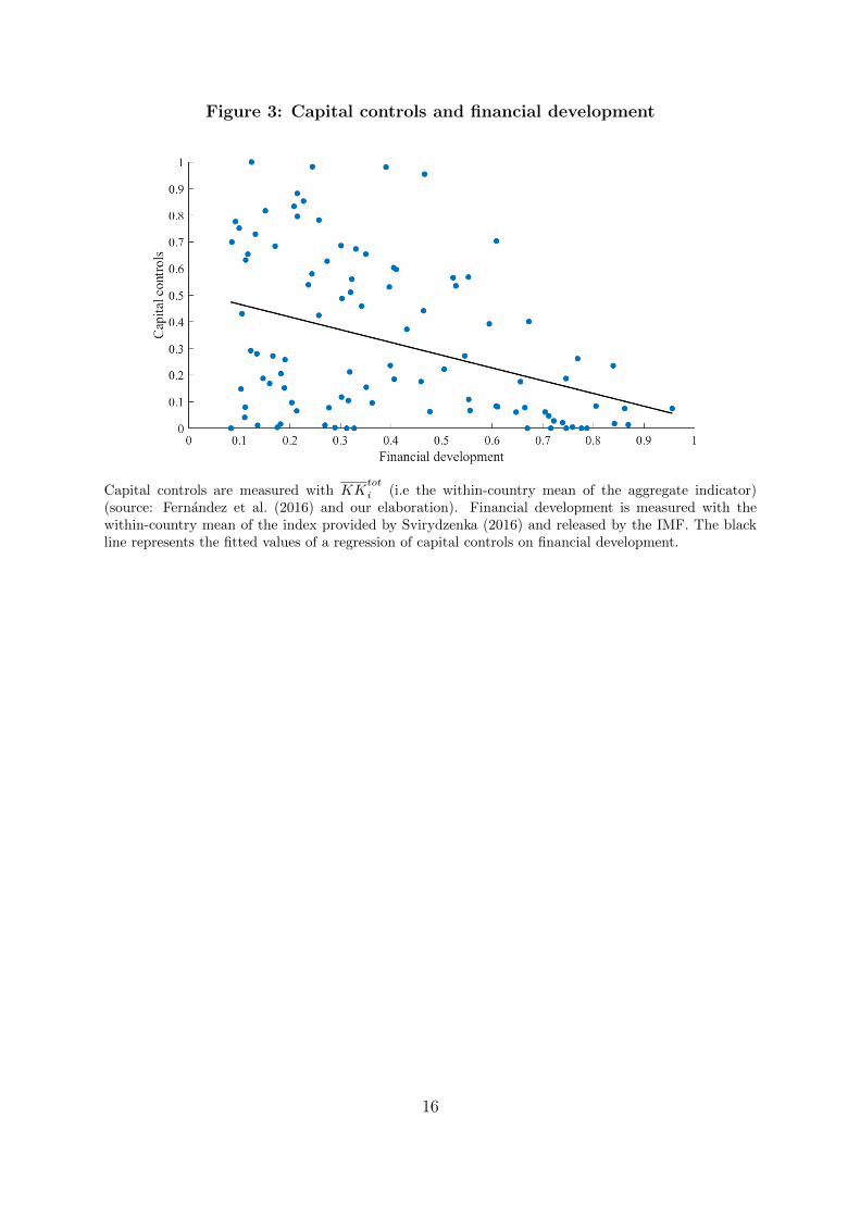
Figure 3: Capital controls and financial development

Capital controls are measured with KKtot

i (i.e the within-country mean of the aggregate indicator)(source: Fernandez et al. (2016) and our elaboration). Financial development is measured with thewithin-country mean of the index provided by Svirydzenka (2016) and released by the IMF. The blackline represents the fitted values of a regression of capital controls on financial development.

16

Table 1: Capital controls indices(cross-country means)

Advanced economies Emerging economies

Capital controls 97-15 97-07 08-15 97-15 97-07 08-15

Aggregate indicator 0.10 0.10 0.11 0.40 0.38 0.41

Inflows 0.11 0.10 0.12 0.39 0.38 0.41

FDI 0.15 0.11 0.20 0.33 0.31 0.35

Portfolio 0.13 0.14 0.13 0.45 0.44 0.47

Other investments 0.03 0.04 0.02 0.38 0.38 0.39

Outflows 0.10 0.10 0.11 0.40 0.39 0.42

FDI 0.07 0.06 0.07 0.30 0.30 0.31

Portfolio 0.13 0.12 0.15 0.46 0.43 0.50

Other investments 0.11 0.12 0.11 0.45 0.44 0.47

Capital controls indices in AEs and EMEs. Source: Fernandez et al. (2016) and our elaboration.

Table 2: Country groups

Country Number of Fin. dev. GDP

group countries (EMEs) index per capita (USD)

Pers. open economies 38 (17) 0.51 25,006

Pers. closed economies 25 (25) 0.36 2,885

Switching countries 12 (6) 0.48 15,643

Episodic controls 25 (21) 0.36 11,060

Active countries 50 (34) 0.40 13,091

Non-active countries 50 (35) 0.43 18,648

Total 100 (69) 0.42 15,916

Capital controls indices in several countries groups. Source: Fernandez et al. (2016) and our elaboration.

17

4 Data and regression model

4.1 Dependent variables

The first goal of the work is to verify to what extent capital controls have an effect

on the volume of capital flows. In this regard Forbes and Warnock (2012) argue that it

is important to focus on gross flows instead of net flows, as the latter can mask dramatic

changes in gross flows.15 Before the mid-1990s researchers used to focus on net flows

which roughly mirrored gross inflows. More recently, the literature has stressed that gross

inflows (driven by foreign investors) and gross outflows (driven by domestic investors) tend

to move independently. This entails that the effects of capital controls need to be analyzed

separately for inflows and outflows and this is what we do in this paper. Moreover, in

order to assess the effectiveness of capital controls for capital flow management purposes,

it is also useful to look at the volatility of capital flows. From this perspective, it is crucial

to see whether capital controls affect the probability of extreme episodes, such as capital

surges and capital flights, reflecting dramatic increases of cross border investments.

We consider four categories of gross capital inflows: i) foreign direct investments; ii)

portfolio investments; iii) other investments; and iv) total inflows, which are the sum of

the three components. The same taxonomy is considered for gross capital outflows. The

data come from the IMF Balance of Payments Statistics and are divided by GDP: gross

inflows refer to the entry “net incurrence of liabilities”, while gross outflows refer to “net

acquisition of financial assets”. If controls are effective, we expect that a tightening of

capital controls on a given flow will reduce that flow.

Our second goal is to analyze whether capital controls affect financial stability and ex-

change rates. In principles, an increase in capital controls should i) reduce the probability

of capital inflow surges and capital flights;16 ii) dampen domestic credit growth by curbing

banks’ external borrowing; iii) depreciate the exchange rate by reducing the demand of

domestic currency; iv) decrease the share of bank loans denominated in foreign currency,

by constraining the ability of domestic banks to tap international markets.17 Accord-

ingly, we take as dependent variables in separate regressions: i) capital surges and capital

flights; ii) the growth of domestic credit to the non-financial sector; iii) the exchange rate

15Justification for focusing on gross flows is also provided in Rothenberg and Warnock (2011) andMilesi-Ferretti and Tille (2011).

16Capital controls may also affect the other two categories of extreme events related to capital flows,i.e. stops and retrenchments. As we are interested in assessing capital controls as a tool to deal withlarge and volatile capital flows, we choose to focus on capital surges/flights which are related to excessiveincreasing inflows/outflows. By contrast, in order to prevent stop/retrenchment episodes capital controlsshould avoid that inflows/outflows fell too much below their average. We leave this analysis to futureresearch.

17Data on domestic credit are obtained from the Global Financial Development Database (Cihak etal. 2013). Data on the currency denomination of bank loans come from the World Bank.

18

misalignments; and iv) the fraction of domestic loans denominated in domestic currency.

In our framework capital surges (capital flights) occur when two conditions are jointly

verified in a given year: i) the annual year-over-year increase of the quarterly inflows

(outflows) exceeds the five-year rolling mean by two standard deviations in at least one

quarter during that year, as in Forbes and Warnock (2012); ii) the annual change exceeds

2% of GDP. Since we use annual data in our regression, we convert into annual data

the information on capital surges and flights that is extracted from quarterly data; for

example, if a capital surge occurs in the last quarter of year t and continues in the

first quarter of year t + 1, our dependent variable will take value 1 both in t and t + 1.

According to our definition, we identify capital surges and flights taking into account both

the variability of flows (first condition) and their macroeconomic size (second condition);

the respect of these conditions ensures that capital surges and flights are extreme episodes

from both a statistical and an economic standpoint (see Crystallin et al., 2015). In our

sample, capital surges and flights occur in 6.8% and 6% of our observations respectively.

If we use the definition of Forbes and Warnock (2012), the occurrence of extreme episodes

increases to 9.8% (for surges) and 9.9% (for flights). As expected, the correlation between

our measure of extreme episodes and the one adopted by Forbes and Warnock (2012) is

high (0.84 for surges, 0.78 for flights).

As regards exchange rate misalignments, we rely on the database EQCHANGE re-

leased by the CEPII which is the only public source providing estimates of the exchange

rate equilibrium levels for a large sample of economies (Couharde et al., 2017). Using the

Behavioral Equilibrium Exchange Rate (BEER) approach, they estimate three models

assuming a long-run relationship between real exchange rates and their fundamentals,

namely the level of productivity, net foreign assets, and terms of trade. Exchange rate

misalignments are obtained as the deviations of the effective exchange rate from its equi-

librium level.18 In our regression, as a proxy of exchange rate misalignments we use an

indicator included in the CEPII dataset: the indicator is the average of the estimates

obtained through the three models and with different gauges of effective exchange rates.

4.2 Empirical specification

Following the literature, our baseline specification is a panel regression model without

country fixed effects, given that capital controls display little variation over time; as

Ostry et al. (2012) point out, the inclusion of fixed effects would make difficult to identify

the effect of capital controls on dependent variables. For each category of flows c =

{fdi, ptf, other} and direction d = {in, out}, we estimate the following regression model:

18As regards the computation of the effective exchange rate, there are several methodological optionsconcerning the number of trading country partners and the weighting schemes.

19

Y c,dit = α + βKKc,d

it−1 + γZit−1 + ϑt + εit

where Y c,dit denotes gross capital flows in percentage of GDP, category c, direction d,

in country i, at time t; KKc,dit−1 is the correspondent capital control index, illustrated

in the previous section: hence, for instance, if the dependent variable is FDI outflows

(Y fdi,outit ), the capital controls indicator used in the regression is KKfdi,out

it−1 ; Zit is a set of

pull factors typically considered19 as important determinants of capital flows: a measure

of the real side of the business cycle (real GDP growth), a measure of the nominal side of

the business cycle (the CPI inflation rate), an index of financial development, the public

debt/GDP ratio as a proxy for country risk, the nominal exchange rate depreciation, a

measure of trade integration (the sum of imports and exports divided by GDP) and a

short-term interest rate; ϑt denotes year fixed effects to capture capital flows push factors;

εit is the error term.20

As anticipated in the previous section, the same model is estimated also for five other

dependent variables: i) capital surges and ii) capital flights; iii) domestic credit growth;

iv) exchange rate misalignment; v) the percentage of domestic loans denominated in

foreign currency. In these additional regressions, the capital control index is KKtot,init−1 ,

except for the regression on capital flights, where we use KKtot,outit−1 . Nevertheless, in some

cases we verify our results by using the capital controls indicator on the individual asset

categories. In regressions i) and ii) we use a logistic model, since the regressands are

dummy variables. In regression iv) we drop from the set of regressors the exchange rate

depreciation and we include the first-difference of foreign reserves/GDP ratio and a set of

dummy variables which measure the flexibility of the exchange rate regime;21 moreover,

given that the exchange rate is a fast-moving variable, we use contemporaneous values of

all regressors but capital controls. In regression v) the sample starts in 2008 due to the

availability of the dependent variable.

All variables (except those taking values in the unit interval, as capital controls) are

winsorized at the 2% to dampen the impact of outliers. Standard errors are clustered at

the country level and are robust to heteroskedasticity. As in Beirne and Friedrich (2017),

we exclude small countries, oil exporters and countries from Sub-Saharan Africa (except

South Africa): therefore, the initial sample of 100 countries, for which the capital controls

index is available, is reduced to 65 countries (40 EMEs and 27 AEs). The sample period is

1997-2015, dictated by the availability of the capital control index (starting from 1997 for

19See for instance Bruno et al. (2017) and Beirne and Friedrich (2017).20Data on control variables are obtained from the WEO, except for financial development (Svirydzenka

(2016), released by the IMF) and the policy rate (Datastream).21The dummy variables are provided by Ilzetzki et al. (2017), which classify countries in six categories

according to the flexibility of the exchange rate.

20

the capital controls on portfolio inflows) and the financial development indicator (which

ends in 2014 and enters the regression with a one-year lag).

Endogeneity issues, in particular reverse causality, are a possible concern in regressions

testing the effectiveness of capital controls. In order to address endogeneity concerns,

capital controls indicators enter the model with a one-year lag. Furthermore, we note that

if countries tend to tighten capital restrictions when the volume of capital flows is high,

or credit excessively grows or when the exchange rate is overvalued, the OLS estimates

of our regression should be upward biased: as a consequence, if the coefficient on capital

controls is estimated to be negative, reverse causality would make the result more robust.

This observation has led many authors to employ an OLS regression when testing the

effectiveness of capital controls, thus downplaying the endogeneity issue.22 Clearly, we

do not want to claim that this is identification is completely clean. Nevertheless, we are

confident that our results help to assess the effectiveness of capital controls.

5 Results

5.1 Baseline specification

In this section we report and comment the estimation results obtained with our em-

pirical model, for each dependent variable. The first set of regressions suggests that

capital controls reduce the volume of capital inflows for all types of investments (table

3): according to the point estimate, a one-standard-deviation increase23 in KKc,init (with

c = fdi, ptf, other) reduces FDI, portfolio and other inflows in percent of GDP by 0.65,

0.45 and 0.7 percentage points respectively.24 Notably, a one-standard-deviation rise in

the aggregate indicator KKtot,in curbs total capital inflows in percent of GDP by 2.29

percentage points (corresponding to 21% of average total inflows, a number in line with

what we find for the asset class-specific indicators). The signs of the other coefficients

are in most cases reasonable, though not always significant. In particular, we find that

capital flows are positively associated with a higher degree of trade openness, financial

development, GDP growth, and interest rates, while higher public debt and exchange

rate depreciation tend to reduce capital inflows. The inflation rate is positively asso-

ciated with higher other inflows, while the estimated coefficients on FDI and portfolio

inflows are negative but not significantly different from zero.

22For instance, Ostry et al. (2012) and Bruno et al. (2017) make a similar argument.23The standard deviations of these indicators lie between 0.3-0.35, so the effects of a standard-deviation

increase is quite comparable among asset classes. The same holds for controls on capital outflows (theirstandard deviation lies between 0.3-0.4).

24These numbers are economically relevant: FDI, portfolio and other inflows decrease by 15%, 18%and 20% of their respective means.

21

In our second set of regressions, we find that restrictions on portfolio and other invest-

ments lead to reduction in capital outflows (table 4): a one-standard-deviation increase

of our indicators reduces portfolio and other outflows in percent of GDP by 0.83 and

0.87 percentage points respectively (around 29% and 35% of their means respectively).

Instead, controls on FDIs have an impact on the correspondent outflows that is indis-

tinguishable from zero, though the sign of the point estimate is anyway negative. If we

consider total outflows, the impact is around a reduction of 2 percentage points, following

a one-standard-deviation rise (around 24% of capital outflows mean). Regressors have

all the expected sign, except for the interest rate, whose positive sign is more difficult to

interpret.

The findings related to first two sets of regressions suggest that capital controls reduce

the volume of gross capital flows. Another related question is whether capital controls

decrease the probability of capital surges and capital flights. We test this hypothesis in our

third set of regressions. The estimated coefficients on KKtot,in and KKtot,out are negative

and statistically significant in the logit regressions on surges and flights respectively (table

5 and 6, first column). A one-standard-deviation increase in the indicators on average

reduces the probability of surges and flight by 3% and 2% percentage points respectively.

Our results differ from those obtained by Forbes and Warnock (2012) who do not find

a significant effect of capital controls on extreme capital flows episodes. We claim that

the main reason is our different definition of extreme episodes. As discussed in the

previous section, our definition of surges and flights is stricter, because we also require

that the annual change in capital flows exceeds 2% of GDP, in order to focus only on

surges and flights that may have a sizable macroeconomic impact. When we use the same

methodology of Forbes and Warnock (2012) to detect surges and flights, the coefficients of

capital controls are no longer significant. This suggests that capital controls are effective

in reducing the probability of extreme episodes only when changes in capital flows are

important from a macroeconomic perspective.

Another rationale for the implementation of capital controls is to avoid that capital

inflows fuel credit booms which can undermine financial stability. In this regard capital

controls may help to mitigate the expansion of domestic credit. Consistently with this

hypothesis, we find a significant effect on domestic credit growth only when we use the

control on other inflows, which include bank loans (table 7, first column): a one-standard-

deviation increase in controls on other inflows reduces credit growth by 1.3 percentage

points.

Next, we assess whether capital controls lead to a reduction in the fraction of domestic

loans denominated in foreign currency on the total domestic loans. Higher capital controls

reduce the ability of domestic banks to tap international markets and hence reduce the

22

amount of foreign currency loans within the economy. On top of that, capital controls

reduce also the ability of domestic agents to borrow directly from foreign banks. This

is what we find in our estimated model (table 8, first column): the sign on KKtot,in

is negative and statistically significant at the 1% level. Notably, the same holds for all

categories of inflows controls. In particular, a one-standard-deviation increase in KKtot,in

is associated with a reduction in foreign currency loans by about 13 percentage points.

Fratzscher (2012) and Pasricha (2017) point out that capital controls may be associ-

ated with mercantilist purposes, i.e. targeting the exchange rate in order to gain compet-

itiveness in international trade. Then we estimate a regression in which the dependent

variable is an indicator of exchange rate misalignment and the regressor of interest is

KKtot,in. Our findings suggest that capital controls on inflows significantly affect the

level of exchange rate misalignment given by the difference between the effective ex-

change rate and its equilibrium level (table 9, first column): a one-standard-deviation

increase in KKtot,in reduces the effective exchange rate by 7% respect to the equilibrium

level.

5.2 Robustness analysis

In the empirical literature on the effectiveness of capital controls, results are mixed

and hinge on several factors. The robustness of our results to the sample composition

is a crucial aspect of our analysis since in the regression model we do not account for

country fixed effects.25 The reason is the little variation in our variable of interest within

individual countries, since many economies tend to not vary the level of capital controls.

As noticed by Eichengreen and Rose (2014), capital controls are persistent: once imposed,

they tend to stay in place for long periods, once removed, they are rarely restored. Aware

of this problem, in this section we put our estimation through some robustness checks

in which we split the sample or exclude some countries, in order to verify whether the

results of baseline regressions can be generalized or, alternatively, they are driven by

some specific economies. In particular, we run regressions separately for AEs and EMEs.

Another check is carried out by excluding from the sample those countries that we have

classified as persistently closed economies: as Klein (2012) points out, it is important

to distinguish between long-standing and episodic capital controls since they respond

to distinct policy objectives and the effects on financial variables tend to be different.

Moreover, given that a large fraction of countries tends to constantly maintain the capital

25In an additional robustness check, we also include region fixed effects. The main results do notchange, the coefficient of interest always keeps the expected sign, even if in some regressions it losessignificance. In particular, while we still find that capital controls reduce total inflows and total outflows,the effect on some components is not significant anymore. The correspondent tables are available uponrequest.

23

controls’ policy stance, we carry out regressions considering only active countries, that

is those countries that tend to change the capital controls stance more frequently (table

A.3 provides details on the composition of the sub-samples). Tables with the estimated

coefficients are reported in the next pages (tables 5-9) and in the Appendix (tables A.4-

A.11).

As regards the effect of capital controls on aggregate inflows, our robustness analysis

confirms the result of the baseline regression. The coefficient on KKtot,in is always nega-

tive and significant (table A.4). The coefficient is much higher for AEs (table A.4, column

3), given that these countries on average receive larger capital flows. When we exclude

persistently closed economies or we consider only active countries, the effectiveness of

capital controls continues to hold (table A.4, column 4 and 5).

We repeat the same exercise for FDI, portfolio and other inflows. With regard to

FDIs, the results of the baseline regression are generally confirmed, except for AEs for

which the coefficient is negative but the p-value is slightly above the 10% threshold

(table A.5, column 3). The effect of capital controls on portfolio investments is always

of the expected sign but strongly significant only for EMEs (table A.6, column 2). For

other investments, we find that the effect of capital controls is significant only for AEs

(table A.7, column 3). To sum up, the effects of capital controls on specific investment

types tend to be differentiated: controls on FDIs reduce inflows across-the-board, those

on portfolio investments are effective only for EMEs, while those on other investments

mainly affect inflows in AEs. In the last two cases the results of the baseline regression

become not significant when we exclude persistently closed economies.

With regard to outflows, the effects of capital controls are more evident for AEs and

are mainly driven by portfolio and other investment (tables A.10-A.11, column 3). For

EMEs, controls on outflows tend to be effective for FDIs, portfolio but not for the other

investments and for the aggregate indicator (tables from A.9 to A.11, column 2). By

excluding persistently closed economies or by considering only active countries, results

are unchanged.

The baseline regressions indicate that capital controls on inflows reduce the probability

of surges. This finding is confirmed for AEs (table 5, column 3) while the effect is not

significant for EMEs (table 5, column 2). The effect is also significant when we restrict the

sample to active countries and when we exclude persistently closed economies (table 5,

column 4 and 5). Analogously, controls on outflows are associated with a lower incidence

of capital flights; this finding holds for both AEs and EMEs (table 6, columns 2 and

3). Nevertheless, the coefficient loses significance when we exclude persistently closed

economies (table 6, column 4).

As regards curbing domestic credit growth, we find that capital controls on other

24

investments are effective for AEs but not for EMEs (table 7, columns 2 and 3). More-

over, we do not find significant effects when we exclude persistently closed economies or

we restrict the sample to active countries (table 7, columns 4 and 5). Accordingly, our

baseline result that capital controls dampen domestic credit growth is mostly driven by

AEs and persistently closed countries. Note that this last finding is not due to the fact

that credit dynamics are slower in closed economies; indeed, on average credit growth in

persistently closed economies (12.3%) is not very different from credit growth in other

countries (11.4% on average); the credit expansion was even more pronounced in India

and China (respectively 14.8 and 17.4%), both persistently closed economies. Our anal-

ysis does not support the use of episodic capital controls to dampen credit expansion,

since the association with credit growth is not significant when we drop countries with

long-standing capital controls. In this regard Klein (2012), using a different dataset on a

smaller sample, finds that the significant association between long-standing capital con-

trols and credit growth disappears when controlling for income per capita. By contrast,

our results are confirmed when we include income per capita suggesting that our estimates

are not biased by this omitted variable. To sum up, the results of the robustness analysis

are not univocal, suggesting that the effects of capital controls on domestic credit, while

robust for some countries, are not systematic.

The robustness analysis indicates that capital controls unambiguously reduce the frac-

tion of loans denominated in foreign currency (table 8). This finding confirms that capital

controls can help to reduce the currency mismatch of the economy, by reducing the volume

of liabilities denominated in foreign currency.

Finally, the baseline regressions indicate that capital controls are associated with

undervalued exchange rates. This outcome is confirmed for EMEs but not for AEs (table

9, columns 2 and 3). Our findings support the argument of several authors that there

may be also mercantilist purposes behind the use of capital controls by some EMEs. The

effect is robust also when we exclude persistently closed economies and when we consider

only active countries (table 9, columns 4 and 5).

25

Table 3: Capital inflows

(1) (2) (3) (4)

Panel Total FDI Portfolio Other

OLS inflows inflows inflows inflows

Capital contr. (tot in) -7.903***

(0.004)

Capital contr. (FDI in) -2.240**

(0.025)

Capital contr. (ptf in) -1.289**

(0.023)

Capital contr. (other in) -1.859*

(0.099)

Growth 0.558** 0.0755 0.0250 0.305

(0.023) (0.377) (0.691) (0.108)

Fin. development 14.15*** 1.468 6.603*** 5.265**

(0.002) (0.352) (0.000) (0.036)

Public debt -0.0274 -0.00321 -0.00956 -0.0113

(0.256) (0.733) (0.228) (0.469)

Trade openness 0.107*** 0.0616*** 0.00359 0.0346***

(0.000) (0.000) (0.620) (0.002)

Inflation 0.0260 -0.0720 -0.0485 0.161*

(0.850) (0.282) (0.197) (0.073)

Depreciation -0.0185 -0.0174 -0.00303 -0.0119

(0.731) (0.384) (0.821) (0.747)

Short-term int. rate 0.173 0.131* 0.0226 -0.0345

(0.280) (0.061) (0.586) (0.713)

Constant -4.086 -0.912 0.0547 -2.547

(0.242) (0.455) (0.954) (0.122)

Observations 885 892 892 885

Countries 65 65 65 65

R2 0.376 0.413 0.239 0.202

Year FE Yes Yes Yes Yes

Robust p-values in parentheses, *** p<0.01, ** p<0.05, * p<0.1.

26

Table 4: Capital outflows

(1) (2) (3) (4)

Panel Total FDI Portfolio Other

OLS outflows outflows outflows outflows

Capital contr. (tot out) -5.621***

(0.009)

Capital contr. (FDI out) -0.616

(0.393)

Capital contr. (ptf out) -2.019***

(0.001)

Capital contr. (other out) -2.124**

(0.020)

Growth 0.286 -0.0454 -0.0378 0.350**

(0.216) (0.601) (0.638) (0.038)

Fin. development 23.76*** 9.548*** 6.911*** 6.999***

(0.000) (0.000) (0.000) (0.001)

Public debt -0.0470** -0.0123 -0.00822 -0.0288*

(0.035) (0.246) (0.321) (0.070)

Trade openness 0.129*** 0.0518*** 0.0430*** 0.0342***

(0.000) (0.000) (0.000) (0.000)

Inflation -0.00166 -0.0369 -0.0498 0.0857

(0.991) (0.294) (0.286) (0.425)

Depreciation 0.0332 -0.0107 -0.00776 0.0466

(0.501) (0.597) (0.681) (0.147)

Short-term int. rate 0.157 0.0897* 0.0212 0.0366

(0.380) (0.081) (0.692) (0.748)

Constant -11.20*** -5.204*** -2.564** -3.241

(0.001) (0.001) (0.014) (0.115)

Observations 880 891 887 885

Countries 65 65 65 65

R2 0.462 0.396 0.455 0.237

Year FE Yes Yes Yes Yes

Robust p-values in parentheses, *** p<0.01, ** p<0.05, * p<0.1.

27

Table 5: Capital surges

(1) (2) (3) (4) (5)

Logit Entire EMEs AEs No pers. Active

surges sample closed

Capital contr. (tot in) -1.601** -0.617 -6.850*** -2.813** -2.887***

(0.015) (0.462) (0.001) (0.045) (0.008)

Growth 0.0817 -0.0469 0.158 0.0677 0.128

(0.234) (0.635) (0.203) (0.430) (0.206)

Fin. development 0.491 0.0918 1.442 0.839 1.414

(0.499) (0.959) (0.302) (0.281) (0.225)

Public debt -0.00159 -0.0199** 0.00677 -0.000733 -0.00622

(0.684) (0.011) (0.158) (0.855) (0.345)

Trade openness 0.000755 0.0118 -0.00158 0.000335 0.0114**

(0.685) (0.154) (0.507) (0.865) (0.025)

Inflation 0.0702** 0.0212 0.271** 0.0738* 0.0564

(0.047) (0.655) (0.033) (0.097) (0.208)

Depreciation -0.0586* -0.0733 -0.102** -0.0755* -0.0223

(0.069) (0.103) (0.028) (0.060) (0.599)

Short-term int. rate 0.00613 0.0903* 0.140 0.0283 0.0114

(0.864) (0.100) (0.281) (0.476) (0.818)

Constant -2.967** -2.686* -4.279* -2.940** -3.588***

(0.024) (0.065) (0.065) (0.041) (0.004)

Observations 579 218 246 477 213

Countries 65 37 28 53 29

Pseudo R2 0.147 0.234 0.141 0.161 0.205

Year FE Yes Yes Yes Yes Yes

Robust p-values in parentheses, *** p<0.01, ** p<0.05, * p<0.1.

28

Table 6: Capital flights

(1) (2) (3) (4) (5)

Logit Entire EMEs AEs No pers. Active

flights sample closed

Capital contr. (tot out) -1.249** -2.077*** -4.067** -0.947 -1.531**

(0.027) (0.007) (0.030) (0.258) (0.042)

Growth 0.0803 0.152 0.00585 0.0890 0.129

(0.272) (0.128) (0.967) (0.249) (0.315)

Fin. development 0.342 3.126** -1.268 0.310 0.323

(0.598) (0.049) (0.153) (0.654) (0.723)

Public debt -0.00695 -0.0265*** -0.00387 -0.00591 -0.00536

(0.105) (0.001) (0.428) (0.146) (0.376)

Trade openness 0.00141 0.0253*** -0.00106 0.000284 0.0157***

(0.516) (0.000) (0.688) (0.892) (0.005)

Inflation 0.00460 -0.0868** 0.0176 0.0100 -0.0104

(0.882) (0.030) (0.882) (0.787) (0.810)

Depreciation 0.00371 0.0503* 0.00979 -0.00422 0.0179

(0.872) (0.094) (0.787) (0.881) (0.526)

Short-term int. rate 0.000760 0.0827** -0.00155 0.00628 -0.00565

(0.980) (0.017) (0.988) (0.826) (0.910)

Constant -2.220** -3.547** -1.284 -2.116** -2.870*

(0.031) (0.041) (0.379) (0.047) (0.069)

Observations 721 300 265 592 308

Countries 65 37 28 53 29

Pseudo R2 0.113 0.264 0.112 0.128 0.142

Year FE Yes Yes Yes Yes Yes

Robust p-values in parentheses, *** p<0.01, ** p<0.05, * p<0.1.

29

Table 7: Credit growth

(1) (2) (3) (4) (5)

Panel OLS Entire EMEs AEs No pers. Active

Credit growth sample closed

Capital contr. (other in) -3.710** -2.436 -9.909*** -0.781 -2.765

(0.031) (0.180) (0.001) (0.802) (0.242)

Growth 1.436*** 1.410*** 1.617*** 1.495*** 1.644***

(0.000) (0.000) (0.000) (0.000) (0.000)

Fin. development -4.860 -8.202 -2.257 -5.168 -10.64*

(0.188) (0.281) (0.705) (0.202) (0.064)

Public debt -0.0468*** -0.0735* -0.0343* -0.0350** -0.0225

(0.003) (0.070) (0.063) (0.019) (0.499)

Trade openness 0.00209 0.0741** -0.0132** -0.00371 0.0265

(0.818) (0.034) (0.042) (0.596) (0.422)

Inflation 0.774*** 0.553*** 2.095*** 0.900*** 0.827***

(0.000) (0.002) (0.003) (0.000) (0.009)

Depreciation -0.328*** -0.355*** -0.292** -0.379*** -0.308**

(0.000) (0.004) (0.014) (0.000) (0.011)

Short-term int. rate -0.132 0.174 -0.582 -0.308* -0.147

(0.431) (0.403) (0.244) (0.078) (0.536)

Constant 8.948*** 4.714 6.185 8.979*** 8.276

(0.003) (0.156) (0.262) (0.008) (0.101)

Observations 886 444 442 724 418

Countries 65 37 28 53 29

R2 0.474 0.445 0.573 0.498 0.560

Year FE Yes Yes Yes Yes Yes

Robust p-values in parentheses, *** p<0.01, ** p<0.05, * p<0.1.

30

Table 8: % FX denominated loans

(1) (2) (3) (4) (5)

Panel OLS Entire EMEs AEs No pers. Active

FX Loans sample closed

Capital contr. (tot in) -45.96*** -50.14*** -78.88** -47.81*** -47.86**

(0.000) (0.000) (0.021) (0.000) (0.040)

Growth -0.0702 -0.651 -0.0210 0.134 0.539

(0.896) (0.217) (0.982) (0.828) (0.452)

Fin. development -27.46* -40.20* 2.610 -25.53 -37.98

(0.093) (0.089) (0.908) (0.135) (0.143)

Public debt 0.00675 0.473*** -0.0810 0.00544 0.0783

(0.945) (0.000) (0.369) (0.956) (0.478)

Trade openness 0.0683** 0.0996 0.0409 0.0734** 0.240

(0.030) (0.268) (0.388) (0.036) (0.165)

Inflation 0.722 1.210** 2.056 0.591 1.033

(0.335) (0.046) (0.143) (0.579) (0.143)

Depreciation -0.101 0.00852 -0.0639 -0.253 0.0463

(0.537) (0.956) (0.859) (0.135) (0.678)

Short-term int. rate 1.403 -1.041 5.790 1.600 1.597

(0.279) (0.143) (0.344) (0.260) (0.239)

Constant 41.24*** 42.27*** 20.36 39.37*** 29.93

(0.001) (0.003) (0.193) (0.002) (0.170)

Observations 291 155 136 262 142

Countries 43 24 19 38 20

R2 0.368 0.670 0.416 0.367 0.446

Year FE Yes Yes Yes Yes Yes

Robust p-values in parentheses, *** p<0.01, ** p<0.05, * p<0.1.

31

Table 9: Ex. Rate misalignment

(1) (2) (3) (4) (5)

Panel OLS Entire EMEs AEs No pers. Active

EX rate mis. sample closed

Capital contr. (tot in) -0.242*** -0.267** 0.0424 -0.331** -0.328***

(0.001) (0.010) (0.808) (0.030) (0.005)

Growth -0.0144*** -0.00952* -0.0122*** -0.0192*** -0.0155**

(0.001) (0.096) (0.000) (0.001) (0.018)

Fin. Development -0.191** -0.409 -0.253*** -0.238** -0.303*

(0.042) (0.115) (0.001) (0.029) (0.077)

Trade openness -0.000449 -0.00155 -0.000186 -0.000364 -0.00168

(0.162) (0.236) (0.188) (0.261) (0.241)

Inflation 0.00999 0.0113 -0.0121* 0.0113 0.0164

(0.263) (0.194) (0.072) (0.257) (0.140)

Short-term int. rate -0.0155 -0.0178 -0.00380 -0.0164 -0.0221*

(0.143) (0.104) (0.562) (0.134) (0.095)

Reserves -0.00350 -0.00610* 0.000635 -0.00483 -0.00905***

(0.270) (0.075) (0.678) (0.197) (0.009)

Constant 0.00585 0.133 0.291*** 0.0485 0.255

(0.973) (0.550) (0.000) (0.831) (0.275)

Observations 894 439 455 738 415

Countries 65 37 28 53 29

R2 0.254 0.292 0.302 0.236 0.315

Year FE Yes Yes Yes Yes Yes

Regime dummies Yes Yes Yes Yes Yes

Robust p-values in parentheses, *** p<0.01, ** p<0.05, * p<0.1.

32

6 Conclusions

This paper has analyzed the effectiveness of capital controls in reducing the volume

and the volatility of capital flows as well as in affecting credit growth, currency loans and

exchange rate misalignment. Our results suggest that inflows controls significantly reduce

capital inflows and tend to reduce the probability of a capital surge, make the exchange

rate more undervalued in emerging markets and decrease the share of loans denominated

in foreign currency. Moreover, we find that restrictions on outflows decrease the volume

of capital outflows in advanced countries and lower the probability of a capital flight.

Notably, we find that effectiveness of capital controls is highly heterogeneous either across

countries and across asset classes. In particular, credit growth seems to respond only to

capital controls on other investments and only in advanced economies.Our outcomes are

similar to some related papers finding that capital controls can play a role in preserving

financial stability.

However, in our view capital controls do not constitute a one-size-fits-all tool and

their usefulness depends both on the objective and the degree of liberalization. In par-

ticular, in line with the IMF Institutional View, we claim that policy makers should not

resort to capital controls in order to avoid the necessary financial reforms and warranted

macroeconomic adjustment.

Moreover, our results should be weighed against the unintended consequences of the

use of capital controls for mercantilist purposes. The strong association between capi-

tal controls and exchange rate misalignments that we document in this paper, chimes

with OECD warnings about the risks related to a widespread use of capital controls.26

Capital controls and exchange rate targeting while potentially beneficiary on short-term

at country level, can lead to negative outcomes from a collective perspective, vanishing

the benefits associated with global financial markets. The multitude of policy objectives

associated with capital controls and the risk of a non-cooperative approach by individ-

ual countries call for a strengthened coordination at international level through the role

played by multilateral organizations such as the IMF and the OECD. “Countering the

risk that process of [trade and] financial integration may go into reverse, requires, above

all, political leadership and international coordination. But co-operation can also greatly

benefit from a clear and globally recognized framework” (Visco 2016).27

We think that the effectiveness of capital controls could be further analyzed, in at

least two dimensions. First, capital controls may potentially affect variables that are

26See for example OECD (2017), “Open and Orderly Capital Movements - Interventions from the2016 OECD High-Level Seminar”.

27Intervention by Ignazio Visco, Governor of the Central Bank of Italy to the “OECD High-LevelSeminar Open and Orderly Capital Movements”.

33

strongly related each other; moreover, their effect is likely to last for some periods. These

considerations could support the use of vector autoregression which, however, require

observations at least at the quarterly frequency.28 Second, an important step further

would be to develop an indicator able to capture not only the extensive margin, but,

more importantly, the change in the intensity of capital controls. We leave these issues

to future research.

28Pasricha et al. (2015) make some steps in this direction.

34

Bibliography

Baba, C. and Kokenyne, A. (2011). Effectiveness of capital controls in selected emerging

markets in the 2000s. IMF Working Paper, (11/281).

Beirne, J. and Friedrich, C. (2017). Macroprudential policies, capital flows, and the

structure of the banking sector. Journal of International Money and Finance, 75: 47–68.

Binici, M., Hutchison, M., and Schindler, M. (2010). Controlling capital? Legal restric-

tions and the asset composition of international financial flows. Journal of International Money and Finance, 29(4): 666–684.

Blundell-Wignall, A. and Roulet, C. (2014). Capital controls on inflows, the global finan-

cial crisis and economic growth. OECD Journal: Financial Market Trends, 2013(2): 29–42.

Bruno, V., Shim, I., and Shin, H. S. (2017). Comparative assessment of macroprudential

policies. Journal of Financial Stability, 28: 183–202.

Caldera Sanchez, A. and Gori, F. (2016). Can Reforms Promoting Growth Increase

Financial Fragility? OECD Economics Department Working Papers, (No. 1340).

Cerutti, E., Claessens, S., and Ratnovski, L. (2014). Global liquidity and drivers of

cross-border bank flows. IMF Working Papers, (14/69).

Chamon, M. and Garcia, M. (2016). Capital Controls in Brazil: Effective? Journal of

International Money and Finance, 61: 163–187.

Couharde, C., Delatte, A.-L., Grekou, C., Mignon, V., and Morvillier, F. (2017).

Eqchange: A world database on actual and equilibrium effective exchange rates. CEPII

Working Paper, (2017-14).

Crystallin, M., Efremidze, L., Kim, S., Nugroho, W., Sula, O., and Willett, T. (2015).

How common are capital flows surges? how they are measured matters-a lot. Open Economies Review, 26(4): 663–682.

Dell’Erba, S. and Reinhardt, D. (2015). FDI, debt and capital controls. Journal of

International Money and Finance, 58: 29–50.

Edwards, S. (2009). Capital controls and capital flows in emerging economies: policies,

practices, and consequences. University of Chicago Press.

35

Eichengreen, B. and Rose, A. (2014). Capital controls in the 21st century. Journal of

International Money and Finance, 48: 1–16.

Fernandez, A., Klein, M. W., Rebucci, A., Schindler, M., and Uribe, M. (2016). Capital

control measures: A new dataset. IMF Economic Review, 64(3): 548–574.

Forbes, K., Fratzscher, M., and Straub, R. (2015). Capital-flow management measures:

What are they good for? Journal of International Economics, 96: S76–S97.

Forbes, K. J. and Warnock, F. E. (2012). Capital flow waves: Surges, stops, flight, and

retrenchment. Journal of International Economics, 88(2): 235–251.

Fratzscher, M. (2012). Capital controls and foreign exchange policy. Journal Economia

Chilena (The Chilean Economy), 15(2): 66–98.

Habermeier, M. K. F., Kokenyne, A., and Baba, C. (2011). The effectiveness of capital

controls and prudential policies in managing large inflows. IMF Staff Position Notes,

(11-14).

Hoggarth, G., Jung, C., and Reinhardt, D. (2016). Capital inflows: the good, the bad

and the bubbly. Bank of England, Financial Stability Paper, (40).

Ilzetzki, E., Reinhart, C. M., and Rogoff, K. S. (2017). Exchange arrangements entering

the 21st century: Which anchor will hold? NBER Working Paper, (w23134).

IMF (2012). The liberalization and management of capital flows: an institutional View.

IMF Staff Paper.

IMF-FSB-BIS (2016). Elements of effective macroprudential policies: Lessons from in-

ternational experience. Technical report.

Klein, M. W. (2012). Capital controls: Gates versus walls. NBER Working Paper,

(18526).

Krugman, P. (1999). Depression economics returns. Foreign Affairs, 78(1): 56–74.

Magud, N. E., Reinhart, C. M., and Rogoff, K. S. (2011). Capital controls: myth and

reality-a portfolio balance approach. NBER Working Paper, (16805).

Milesi-Ferretti, G.-M. and Tille, C. (2011). The great retrenchment: international capital

flows during the global financial crisis. Economic policy, 26(66): 289–346.

OECD (2017). Open and Orderly Capital Movements: Interventions from the 2016 OECD

High-Level Seminar.

36

Ostry, J. D., Ghosh, A. R., Chamon, M., and Qureshi, M. S. (2012). Tools for manag-

ing financial-stability risks from capital inflows. Journal of International Economics, 88(2): 407–421.

Ostry, J. D., Ghosh, A. R., Habermeier, K., Chamon, M., Qureshi, M. S., and Reinhardt,

D. (2010). Capital inflows: The role of controls. IMF Staff Position Notes, (04).

Pasricha, G. (2017). Policy rules for capital controls. BIS Working Papers, (670).

Pasricha, G., Falagiarda, M., Bijsterbosch, M., and Aizenman, J. (2015). Domestic and

Multilateral Effects of Capital Controls in Emerging Markets. NBER Working Paper,

(w20822).

Quinn, D., Schindler, M., and Toyoda, A. M. (2011). Assessing measures of financial

openness and integration. IMF Economic Review, 59(3): 488–522.

Rey, H. (2015). Dilemma not Trilemma: the Global Cycle and Monetary Policy Indepen-

dence. NBER Working Paper, (No. 21162).

Rodrik, D. (1998). Who needs capital-account convertibility? Essays in International

Finance, pages 55–65.

Rothenberg, A. D. and Warnock, F. E. (2011). Sudden flight and true sudden stops.

Review of International Economics, 19(3): 509–524.

Schindler, M. (2009). Measuring financial integration: A new data set. IMF Staff Papers,

56(1): 222–238.

Svirydzenka, K. (2016). Introducing a new broad-based ndex of financial development.

IMF Working Paper, (16/5).

Vithessonthi, C. and Tongurai, J. (2013). Unremunerated Reserve Requirements, Ex-

change Rate Volatility, and Firm Value. Journal of International Financial Markets, Institutions and Money, 23: 358–378.

37

Appendix

A.1 Additional tables

Table A.1: Aggregation of capital controls dummies

Capital control Dummy restrictions Dummy restrictions

by investment on specific transactions: on specific transactions:

type capital inflows capital outflows

FDIDirect investment inflows Direct investment outflows

Direct investment liquidation Direct investment liquidation

Portfolio

Equity (purchase locally by non residents) Equity (purchase abroad by res.)

Equity (sale or issue locally by non res.) Equity (sale or issue abroad by res.)

Bond (purchase locally by non res.) Bond (purchase abroad by res.)

Bond (sale or issue locally by non res.) Bond (sale or issue abroad by res.)

Money market instruments Money market instruments

(purchase locally by non res.) (purchase abroad by res.)

Money market instruments Money market instruments

(sale or issue locally by non res.) (sale or issue abroad by res.)

Collective investments Collective investments

(purchase locally by non res.) (purchase abroad by res.)

Collective investments Collective investments

(sale or issue locally by non res.) (sale or issue abroad by res.)

Other investment

Financial credits inflows Financial credits outflows

Commercial credits inflows Commercial credits outflows

Guarantees, sureties and Guarantees, sureties and

financial backup facilities inflows financial backup facilities outflows

Dummy variables are taken from Fernandez et al. (2016).

38

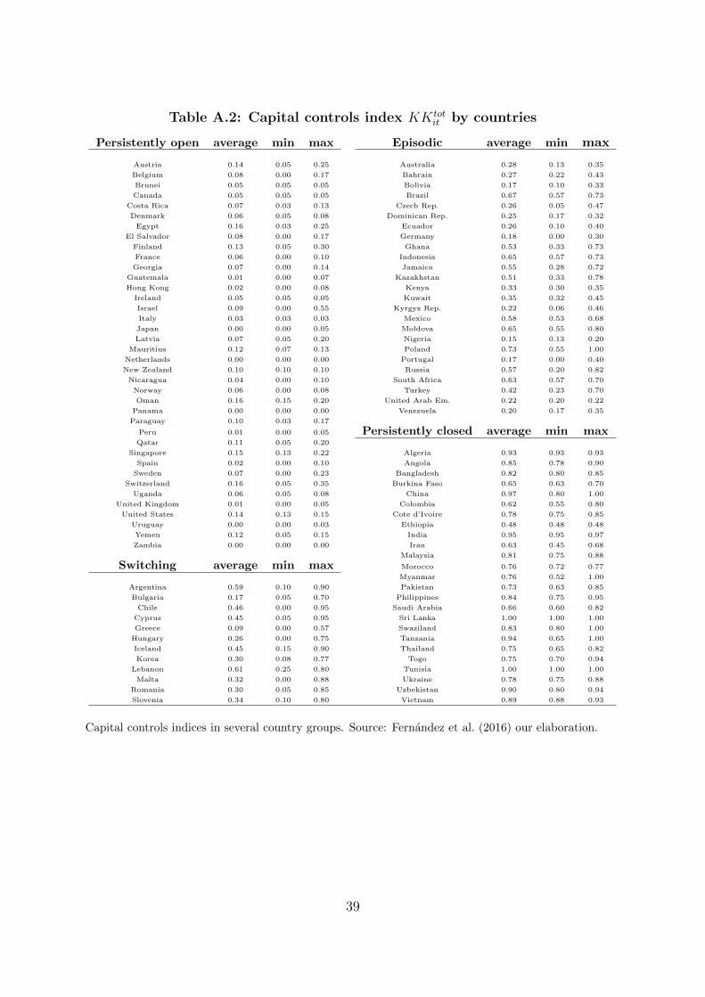
Table A.2: Capital controls index KKtotit by countries

Persistently open average min max Episodic average min max

Austria 0.14 0.05 0.25 Australia 0.28 0.13 0.35

Belgium 0.08 0.00 0.17 Bahrain 0.27 0.22 0.43

Brunei 0.05 0.05 0.05 Bolivia 0.17 0.10 0.33

Canada 0.05 0.05 0.05 Brazil 0.67 0.57 0.73

Costa Rica 0.07 0.03 0.13 Czech Rep. 0.26 0.05 0.47

Denmark 0.06 0.05 0.08 Dominican Rep. 0.25 0.17 0.32

Egypt 0.16 0.03 0.25 Ecuador 0.26 0.10 0.40

El Salvador 0.08 0.00 0.17 Germany 0.18 0.00 0.30

Finland 0.13 0.05 0.30 Ghana 0.53 0.33 0.73

France 0.06 0.00 0.10 Indonesia 0.65 0.57 0.73

Georgia 0.07 0.00 0.14 Jamaica 0.55 0.28 0.72

Guatemala 0.01 0.00 0.07 Kazakhstan 0.51 0.33 0.78

Hong Kong 0.02 0.00 0.08 Kenya 0.33 0.30 0.35

Ireland 0.05 0.05 0.05 Kuwait 0.35 0.32 0.45

Israel 0.09 0.00 0.55 Kyrgyz Rep. 0.22 0.06 0.46

Italy 0.03 0.03 0.03 Mexico 0.58 0.53 0.68

Japan 0.00 0.00 0.05 Moldova 0.65 0.55 0.80

Latvia 0.07 0.05 0.20 Nigeria 0.15 0.13 0.20

Mauritius 0.12 0.07 0.13 Poland 0.73 0.55 1.00

Netherlands 0.00 0.00 0.00 Portugal 0.17 0.00 0.40

New Zealand 0.10 0.10 0.10 Russia 0.57 0.20 0.82

Nicaragua 0.04 0.00 0.10 South Africa 0.63 0.57 0.70

Norway 0.06 0.00 0.08 Turkey 0.42 0.23 0.70

Oman 0.16 0.15 0.20 United Arab Em. 0.22 0.20 0.22

Panama 0.00 0.00 0.00 Venezuela 0.20 0.17 0.35

Paraguay 0.10 0.03 0.17

Peru 0.01 0.00 0.05 Persistently closed average min maxQatar 0.11 0.05 0.20

Singapore 0.15 0.13 0.22 Algeria 0.93 0.93 0.93

Spain 0.02 0.00 0.10 Angola 0.85 0.78 0.90

Sweden 0.07 0.00 0.23 Bangladesh 0.82 0.80 0.85

Switzerland 0.16 0.05 0.35 Burkina Faso 0.65 0.63 0.70

Uganda 0.06 0.05 0.08 China 0.97 0.80 1.00

United Kingdom 0.01 0.00 0.05 Colombia 0.62 0.55 0.80

United States 0.14 0.13 0.15 Cote d’Ivoire 0.78 0.75 0.85

Uruguay 0.00 0.00 0.03 Ethiopia 0.48 0.48 0.48

Yemen 0.12 0.05 0.15 India 0.95 0.95 0.97

Zambia 0.00 0.00 0.00 Iran 0.63 0.45 0.68

Malaysia 0.81 0.75 0.88

Switching average min max Morocco 0.76 0.72 0.77

Myanmar 0.76 0.52 1.00

Argentina 0.59 0.10 0.90 Pakistan 0.73 0.63 0.85

Bulgaria 0.17 0.05 0.70 Philippines 0.84 0.75 0.95

Chile 0.46 0.00 0.95 Saudi Arabia 0.66 0.60 0.82

Cyprus 0.45 0.05 0.95 Sri Lanka 1.00 1.00 1.00

Greece 0.09 0.00 0.57 Swaziland 0.83 0.80 1.00

Hungary 0.26 0.00 0.75 Tanzania 0.94 0.65 1.00

Iceland 0.45 0.15 0.90 Thailand 0.75 0.65 0.82

Korea 0.30 0.08 0.77 Togo 0.75 0.70 0.94

Lebanon 0.61 0.25 0.80 Tunisia 1.00 1.00 1.00

Malta 0.32 0.00 0.88 Ukraine 0.78 0.75 0.88

Romania 0.30 0.05 0.85 Uzbekistan 0.90 0.80 0.94

Slovenia 0.34 0.10 0.80 Vietnam 0.89 0.88 0.93

Capital controls indices in several country groups. Source: Fernandez et al. (2016) our elaboration.

39

Table A.3: Country groups (estimation sample)

Group Entire sample AEs EMEs

Pers. open 31 21 10

Pers. closed 13 0 13

Switching 9 3 6

Episodic 12 4 8

Total 65 37 28

Active 30 18 12

Non-active 35 16 19

Composition of country groups in the estimation sample. Source: our elaboration.

40

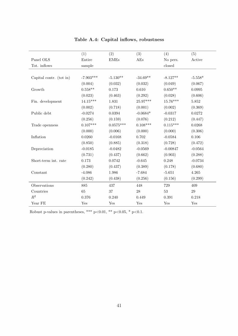
Table A.4: Capital inflows, robustness

(1) (2) (3) (4) (5)

Panel OLS Entire EMEs AEs No pers. Active

Tot. inflows sample closed

Capital contr. (tot in) -7.903*** -5.130** -34.69** -8.127** -5.558*

(0.004) (0.032) (0.032) (0.049) (0.067)

Growth 0.558** 0.173 0.610 0.650** 0.0995

(0.023) (0.463) (0.292) (0.028) (0.606)

Fin. development 14.15*** 1.831 25.97*** 15.76*** 5.852

(0.002) (0.718) (0.001) (0.002) (0.369)

Public debt -0.0274 0.0394 -0.0684* -0.0317 0.0272

(0.256) (0.159) (0.076) (0.212) (0.447)

Trade openness 0.107*** 0.0575*** 0.108*** 0.115*** 0.0268

(0.000) (0.006) (0.000) (0.000) (0.306)

Inflation 0.0260 -0.0168 0.702 -0.0584 0.106

(0.850) (0.885) (0.318) (0.728) (0.472)

Depreciation -0.0185 -0.0482 -0.0569 -0.00847 -0.0564

(0.731) (0.437) (0.662) (0.903) (0.288)

Short-term int. rate 0.173 0.0742 -0.645 0.248 -0.0734

(0.280) (0.437) (0.389) (0.178) (0.680)

Constant -4.086 1.986 -7.684 -5.651 4.265

(0.242) (0.438) (0.256) (0.156) (0.299)

Observations 885 437 448 729 409

Countries 65 37 28 53 29

R2 0.376 0.240 0.449 0.391 0.218

Year FE Yes Yes Yes Yes Yes

Robust p-values in parentheses, *** p<0.01, ** p<0.05, * p<0.1.

41

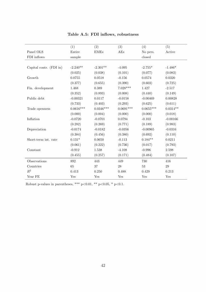
Table A.5: FDI inflows, robustness

(1) (2) (3) (4) (5)

Panel OLS Entire EMEs AEs No pers. Active

FDI inflows sample closed

Capital contr. (FDI in) -2.240** -2.301** -4.095 -2.755* -1.486*

(0.025) (0.038) (0.101) (0.077) (0.083)

Growth 0.0755 0.0518 -0.156 0.0574 0.0320

(0.377) (0.655) (0.390) (0.603) (0.725)

Fin. development 1.468 0.389 7.028*** 1.427 -2.517

(0.352) (0.893) (0.008) (0.440) (0.149)

Public debt -0.00321 0.0117 -0.0158 -0.00469 0.00828

(0.733) (0.403) (0.293) (0.625) (0.611)

Trade openness 0.0616*** 0.0346*** 0.0691*** 0.0655*** 0.0314**

(0.000) (0.004) (0.000) (0.000) (0.018)

Inflation -0.0720 -0.0701 0.0794 -0.103 -0.00166

(0.282) (0.269) (0.771) (0.189) (0.983)

Depreciation -0.0174 -0.0182 -0.0356 -0.00965 -0.0316

(0.384) (0.456) (0.380) (0.692) (0.110)

Short-term int. rate 0.131* 0.0650 -0.113 0.184** 0.0211

(0.061) (0.222) (0.736) (0.017) (0.793)

Constant -0.912 1.538 -4.108 -0.996 2.598

(0.455) (0.257) (0.171) (0.484) (0.107)

Observations 892 443 449 730 416

Countries 65 37 28 53 29

R2 0.413 0.250 0.488 0.429 0.213

Year FE Yes Yes Yes Yes Yes

Robust p-values in parentheses, *** p<0.01, ** p<0.05, * p<0.1.

42

Table A.6: Portfolio inflows, robustness

(1) (2) (3) (4) (5)

Panel OLS Entire EMEs AEs No pers. Active

Ptf. inflows sample closed

Capital contr. (ptf in) -1.289** -0.875** -0.603 -0.742 -1.378

(0.023) (0.044) (0.713) (0.329) (0.105)

Growth 0.0250 0.0366 0.0481 0.0631 0.0115

(0.691) (0.315) (0.790) (0.399) (0.909)

Fin. development 6.603*** 3.036*** 6.288** 6.797*** 6.466***

(0.000) (0.006) (0.035) (0.000) (0.003)

Public debt -0.00956 0.00200 -0.0145 -0.0104 0.000374

(0.228) (0.822) (0.233) (0.191) (0.971)

Trade openness 0.00359 0.00693 0.00234 0.00334 -0.000633

(0.620) (0.137) (0.796) (0.676) (0.927)

Inflation -0.0485 -0.0341 -0.171 -0.0830* -0.0352

(0.197) (0.133) (0.476) (0.072) (0.314)

Depreciation -0.00303 -0.00680 0.0138 0.000960 0.000227

(0.821) (0.503) (0.676) (0.954) (0.990)

Short-term int. rate 0.0226 0.0247 0.0789 0.0231 -0.0147

(0.586) (0.207) (0.736) (0.627) (0.741)

Constant 0.0547 -0.0834 0.901 -0.00353 0.0170

(0.954) (0.874) (0.644) (0.997) (0.988)

Observations 892 443 449 730 416

Countries 65 37 28 53 29

R2 0.239 0.217 0.153 0.215 0.258

Year FE Yes Yes Yes Yes Yes

Robust p-values in parentheses, *** p<0.01, ** p<0.05, * p<0.1.

43

Table A.7: Other inflows, robustness

(1) (2) (3) (4) (5)

Panel OLS Entire EMEs AEs No pers. Active

Other inflows sample closed

Capital contr. (other in) -1.859* -0.644 -14.59*** -2.063 -1.469

(0.099) (0.377) (0.002) (0.205) (0.237)

Growth 0.305 0.0836 0.475 0.406* -0.0404

(0.108) (0.479) (0.341) (0.096) (0.805)

Fin. development 5.265** -3.100 10.19* 5.920** 2.296

(0.036) (0.126) (0.084) (0.038) (0.474)

Public debt -0.0113 0.0199** -0.0221 -0.0118 0.0265

(0.469) (0.030) (0.379) (0.472) (0.146)

Trade openness 0.0346*** 0.0143** 0.0367*** 0.0370*** -0.00798

(0.002) (0.047) (0.010) (0.001) (0.430)

Inflation 0.161* 0.0840 0.726 0.146 0.178

(0.073) (0.213) (0.117) (0.213) (0.128)

Depreciation -0.0119 -0.0286 -0.0265 -0.00406 -0.0389

(0.747) (0.452) (0.751) (0.930) (0.358)

Short-term int. rate -0.0345 0.00106 -0.569 -0.0375 -0.122

(0.713) (0.986) (0.290) (0.745) (0.223)

Constant -2.547 0.623 -5.559 -3.277* 1.561

(0.122) (0.492) (0.206) (0.084) (0.338)

Observations 885 437 448 729 409

Countries 65 37 28 53 29

R2 0.202 0.167 0.300 0.232 0.157

Year FE Yes Yes Yes Yes Yes

Robust p-values in parentheses, *** p<0.01, ** p<0.05, * p<0.1..

44

Table A.8: Capital outflows, robustness

(1) (2) (3) (4) (5)

Panel OLS Entire EMEs AEs No pers. Active

Tot. outflows sample closed

Capital contr. (tot out) -5.621*** -2.120 -16.81** -9.995*** -4.268**

(0.009) (0.181) (0.044) (0.000) (0.028)

Growth 0.286 0.0575 0.0692 0.318 -0.170

(0.216) (0.758) (0.905) (0.258) (0.264)

Fin. development 23.76*** 7.936* 32.22*** 26.39*** 15.82***

(0.000) (0.069) (0.000) (0.000) (0.004)

Public debt -0.0470** -0.0507*** -0.0592* -0.0526** -0.0410**

(0.035) (0.007) (0.066) (0.015) (0.028)

Trade openness 0.129*** 0.0354** 0.153*** 0.138*** 0.00599

(0.000) (0.021) (0.000) (0.000) (0.718)

Inflation -0.00166 -0.0456 -0.320 -0.148 -0.00679

(0.991) (0.588) (0.617) (0.331) (0.957)

Depreciation 0.0332 0.0181 -0.0829 0.0657 0.00947

(0.501) (0.707) (0.515) (0.290) (0.812)

Short-term int. rate 0.157 0.155** -0.773 0.316* 0.00982

(0.380) (0.035) (0.385) (0.075) (0.938)

Constant -11.20*** 0.197 -14.49* -13.13*** 2.091

(0.001) (0.911) (0.068) (0.000) (0.426)

Observations 880 431 449 729 408

Countries 65 37 28 53 29

R2 0.462 0.206 0.489 0.480 0.300

Year FE Yes Yes Yes Yes Yes

Robust p-values in parentheses, *** p<0.01, ** p<0.05, * p<0.1.

45

Table A.9: FDI outflows, robustness

(1) (2) (3) (4) (5)

Panel OLS Entire EMEs AEs No pers. Active

FDI outflows sample closed

Capital contr. (FDI out) -0.616 -0.860* -3.584 -1.981* -1.102*

(0.393) (0.094) (0.132) (0.075) (0.058)

Growth -0.0454 -0.0914 -0.181 -0.0610 -0.0157

(0.601) (0.353) (0.434) (0.575) (0.855)

Fin. development 9.548*** 6.343** 13.71*** 10.20*** 5.803***

(0.000) (0.011) (0.000) (0.000) (0.000)

Public debt -0.0123 0.00724 -0.0321 -0.0154 0.00132

(0.246) (0.247) (0.107) (0.169) (0.864)

Trade openness 0.0518*** 0.0203** 0.0585*** 0.0561*** 0.0192*

(0.000) (0.012) (0.001) (0.000) (0.082)

Inflation -0.0369 -0.00533 -0.115 -0.0646 -0.0509

(0.294) (0.841) (0.610) (0.156) (0.127)

Depreciation -0.0107 -0.0238 -0.0378 -0.000313 -0.0134

(0.597) (0.263) (0.457) (0.990) (0.539)

Short-term int. rate 0.0897* 0.0292 -0.499 0.142** 0.0637

(0.081) (0.215) (0.144) (0.012) (0.185)

Constant -5.204*** -2.179*** -5.688 -5.762*** -2.214**

(0.001) (0.006) (0.130) (0.002) (0.017)

Observations 891 442 449 729 415

Countries 65 37 28 53 29

R2 0.396 0.211 0.387 0.400 0.203

Year FE Yes Yes Yes Yes Yes

Robust p-values in parentheses, *** p<0.01, ** p<0.05, * p<0.1.

46

Table A.10: Portfolio outflows, robustness

(1) (2) (3) (4) (5)

Panel OLS Entire EMEs AEs No pers. Active

Ptf. outflows sample closed

Capital contr. (ptf out) -2.019*** -0.972** -4.377** -2.263*** -1.330**

(0.001) (0.012) (0.023) (0.006) (0.013)

Growth -0.0378 0.0240 -0.441** -0.0707 -0.117

(0.638) (0.372) (0.029) (0.491) (0.109)

Fin. development 6.911*** 3.708*** 7.112** 7.451*** 5.217***

(0.000) (0.005) (0.010) (0.000) (0.000)

Public debt -0.00822 -0.00362 -0.0192 -0.0107 0.00343

(0.321) (0.646) (0.175) (0.202) (0.682)

Trade openness 0.0430*** 0.00512 0.0542*** 0.0469*** -0.00277

(0.000) (0.180) (0.000) (0.000) (0.632)

Inflation -0.0498 -0.0542** -0.393* -0.101* -0.00488

(0.286) (0.016) (0.051) (0.075) (0.907)

Depreciation -0.00776 0.0171* -0.0572 -0.00136 -0.00689

(0.681) (0.086) (0.222) (0.953) (0.742)

Short-term int. rate 0.0212 0.0211 -0.166 0.0620 -0.0555

(0.692) (0.146) (0.491) (0.321) (0.198)

Constant -2.564** -0.181 -0.671 -2.979** 0.874

(0.014) (0.716) (0.832) (0.012) (0.461)

Observations 887 438 449 729 415

Countries 65 37 28 53 29

R2 0.455 0.235 0.444 0.454 0.314

Year FE Yes Yes Yes Yes Yes

Robust p-values in parentheses, *** p<0.01, ** p<0.05, * p<0.1.

47

Table A.11: Other outflows, robustness

(1) (2) (3) (4) (5)

Panel OLS Entire EMEs AEs No pers. Active

Other outflows sample closed

Capital contr. (other out) -2.124** -0.281 -4.628* -4.163*** -1.527

(0.020) (0.767) (0.082) (0.000) (0.198)

Growth 0.350** 0.141 0.730* 0.465** -0.0311

(0.038) (0.247) (0.080) (0.034) (0.658)

Fin. development 6.999*** -1.770 10.90*** 8.624*** 5.057

(0.001) (0.520) (0.003) (0.000) (0.145)

Public debt -0.0288* -0.0574*** -0.00689 -0.0295* -0.0479***

(0.070) (0.008) (0.683) (0.054) (0.006)

Trade openness 0.0342*** 0.00899 0.0395*** 0.0350*** -0.0103

(0.000) (0.382) (0.000) (0.000) (0.230)

Inflation 0.0857 0.0223 0.178 0.0255 0.0554

(0.425) (0.737) (0.630) (0.825) (0.599)

Depreciation 0.0466 0.0274 0.0172 0.0633 0.0284

(0.147) (0.454) (0.846) (0.113) (0.197)

Short-term int. rate 0.0366 0.0978 -0.0854 0.0861 -0.00502

(0.748) (0.113) (0.855) (0.449) (0.950)

Constant -3.241 2.503 -8.348** -4.411** 3.306**

(0.115) (0.108) (0.023) (0.043) (0.049)

Observations 885 436 449 730 409

Countries 65 37 28 53 29

R2 0.237 0.201 0.322 0.265 0.209

Year FE Yes Yes Yes Yes Yes

Robust p-values in parentheses, *** p<0.01, ** p<0.05, * p<0.1.

48

(*) Requests for copies should be sent to: Banca d’Italia – Servizio Studi di struttura economica e finanziaria – Divisione Biblioteca e Archivio storico – Via Nazionale, 91 – 00184 Rome – (fax 0039 06 47922059). They are available on the Internet www.bancaditalia.it.

RECENTLY PUBLISHED “TEMI” (*)

N. 1171 – The potential of big housing data: an application to the Italian real-estate market, by Michele Loberto, Andrea Luciani and Marco Pangallo (April 2018).

N. 1172 – ECB monetary policy and the euro exchange rate, by Martina Cecioni (April 2018).

N. 1173 – Firms’ investments during two crises, by Antonio De Socio and Enrico Sette (April 2018).

N. 1174 – How can the government spending multiplier be small at the zero lower bound?, by Valerio Ercolani and João Valle e Azevedo (April 2018).

N. 1175 – Asset price volatility in EU-6 economies: how large is the role played by the ECB?, by Alessio Ciarlone and Andrea Colabella (June 2018).

N. 1176 – Fixed rate versus adjustable rate mortgages: evidence from euro area banks, by Ugo Albertazzi, Fulvia Fringuellotti and Steven Ongena (June 2018).

N. 1177 – Short term forecasts of economic activity: are fortnightly factors useful?, by Libero Monteforte and Valentina Raponi (June 2018).

N. 1178 – Discretion and supplier selection in public procurement, by Audinga Baltrunaite, Cristina Giorgiantonio, Sauro Mocetti and Tommaso Orlando (June 2018).

N. 1179 – Labor market and financial shocks: a time varying analysis, by Francesco Corsello and Valerio Nispi Landi (June 2018).

N. 1180 – On the unintended effects of public transfers: evidence from EU funding to Southern Italy, by Ilaria De Angelis, Guido de Blasio and Lucia Rizzica (June 2018).

N. 1181 – Always look on the bright side? Central counterparties and interbank markets during the financial crisis, by Massimiliano Affinito and Matteo Piazza (July 2018).

N. 1182 – Knocking on parents’ doors: regulation and intergenerational mobility, by Sauro Mocetti, Giacomo Roma and Enrico Rubolino (July 2018).

N. 1183 – Why do banks securitise their assets? Bank-level evidence from over one hundred countries in the pre-crisis period, by Fabio Panetta and Alberto Franco Pozzolo.

N. 1184 – Capital controls spillovers, by Valerio Nispi Landi (July 2018).

N. 1185 – The macroeconomic effects of an open-ended asset purchase programme, by Lorenzo Burlon, Alessandro Notarpietro and Massimiliano Pisani (July 2018).

N. 1186 – Fiscal buffers, private debt and recession: the good, the bad and the ugly, by Nicoletta Batini, Giovanni Melina and Stefania Villa (July 2018).

N. 1187 – Competition and the pass-through of unconventional monetary policy: evidence from TLTROs, by Matteo Benetton and Davide Fantino (September 2018).

N. 1188 – Raising aspirations and higher education: evidence from the UK’s Widening Participation Policy, by Lucia Rizzica (September 2018).

N. 1189 – Nearly exact Bayesian estimation of non-linear no-arbitrage term structure models, by Marcello Pericoli and Marco Taboga (September 2018).

N. 1190 – Granular Sources of the Italian business cycle, by Nicolò Gnocato and Concetta Rondinelli (September 2018).

N. 1191 – Debt restructuring with multiple bank relationships, by Angelo Baglioni, Luca Colombo and Paola Rossi (September 2018).

N. 1192 – Exchange rate pass-through into euro area inflation. An estimated structural model, by Lorenzo Burlon, Alessandro Notarpietro and Massimiliano Pisani (September 2018).

N. 1193 – The effect of grants on university drop-out rates: evidence on the Italian case, by Francesca Modena, Enrico Rettore and Giulia Martina Tanzi (September 2018).

"TEMI" LATER PUBLISHED ELSEWHERE

2016

ALBANESE G., G. DE BLASIO and P. SESTITO, My parents taught me. evidence on the family transmission of values, Journal of Population Economics, v. 29, 2, pp. 571-592, WP 955 (March 2014).

ANDINI M. and G. DE BLASIO, Local development that money cannot buy: Italy’s Contratti di Programma, Journal of Economic Geography, v. 16, 2, pp. 365-393, WP 915 (June 2013).

BARONE G. and S. MOCETTI, Inequality and trust: new evidence from panel data, Economic Inquiry, v. 54, pp. 794-809, WP 973 (October 2014).

BELTRATTI A., B. BORTOLOTTI and M. CACCAVAIO, Stock market efficiency in China: evidence from the split-share reform, Quarterly Review of Economics and Finance, v. 60, pp. 125-137, WP 969 (October 2014).

BOLATTO S. and M. SBRACIA, Deconstructing the gains from trade: selection of industries vs reallocation of workers, Review of International Economics, v. 24, 2, pp. 344-363, WP 1037 (November 2015).

BOLTON P., X. FREIXAS, L. GAMBACORTA and P. E. MISTRULLI, Relationship and transaction lending in a crisis, Review of Financial Studies, v. 29, 10, pp. 2643-2676, WP 917 (July 2013).

BONACCORSI DI PATTI E. and E. SETTE, Did the securitization market freeze affect bank lending during the financial crisis? Evidence from a credit register, Journal of Financial Intermediation , v. 25, 1, pp. 54-76, WP 848 (February 2012).

BORIN A. and M. MANCINI, Foreign direct investment and firm performance: an empirical analysis of Italian firms, Review of World Economics, v. 152, 4, pp. 705-732, WP 1011 (June 2015).

BRAGOLI D., M. RIGON and F. ZANETTI, Optimal inflation weights in the euro area, International Journal of Central Banking, v. 12, 2, pp. 357-383, WP 1045 (January 2016).

BRANDOLINI A. and E. VIVIANO, Behind and beyond the (headcount) employment rate, Journal of the Royal Statistical Society: Series A, v. 179, 3, pp. 657-681, WP 965 (July 2015).

BRIPI F., The role of regulation on entry: evidence from the Italian provinces, World Bank Economic Review, v. 30, 2, pp. 383-411, WP 932 (September 2013).

BRONZINI R. and P. PISELLI, The impact of R&D subsidies on firm innovation, Research Policy, v. 45, 2, pp. 442-457, WP 960 (April 2014).

BURLON L. and M. VILALTA-BUFI, A new look at technical progress and early retirement, IZA Journal of Labor Policy, v. 5, WP 963 (June 2014).

BUSETTI F. and M. CAIVANO, The trend–cycle decomposition of output and the Phillips Curve: bayesian estimates for Italy and the Euro Area, Empirical Economics, V. 50, 4, pp. 1565-1587, WP 941 (November 2013).

CAIVANO M. and A. HARVEY, Time-series models with an EGB2 conditional distribution, Journal of Time Series Analysis, v. 35, 6, pp. 558-571, WP 947 (January 2014).

CALZA A. and A. ZAGHINI, Shoe-leather costs in the euro area and the foreign demand for euro banknotes, International Journal of Central Banking, v. 12, 1, pp. 231-246, WP 1039 (December 2015).

CESARONI T. and R. DE SANTIS, Current account “core-periphery dualism” in the EMU, The World Economy, v. 39, 10, pp. 1514-1538, WP 996 (December 2014).

CIANI E., Retirement, Pension eligibility and home production, Labour Economics, v. 38, pp. 106-120, WP 1056 (March 2016).

CIARLONE A. and V. MICELI, Escaping financial crises? Macro evidence from sovereign wealth funds’ investment behaviour, Emerging Markets Review, v. 27, 2, pp. 169-196, WP 972 (October 2014).

CORNELI F. and E. TARANTINO, Sovereign debt and reserves with liquidity and productivity crises, Journal of International Money and Finance, v. 65, pp. 166-194, WP 1012 (June 2015).

D’AURIZIO L. and D. DEPALO, An evaluation of the policies on repayment of government’s trade debt in Italy, Italian Economic Journal, v. 2, 2, pp. 167-196, WP 1061 (April 2016).

DE BLASIO G., G. MAGIO and C. MENON, Down and out in Italian towns: measuring the impact of economic downturns on crime, Economics Letters, 146, pp. 99-102, WP 925 (July 2013).

DOTTORI D. and M. MANNA, Strategy and tactics in public debt management, Journal of Policy Modeling, v. 38, 1, pp. 1-25, WP 1005 (March 2015).

GERALI A., A. NOTARPIETRO and M. PISANI, Macroeconomic effects of simultaneous implementation of reforms, International Finance, Wiley Blackwell, v. 19, 1, pp. 42-65, WP 997 (December 2014).

LIBERATI D., M. MARINUCCI and G. M. TANZI, Science and technology parks in Italy: main features and analysis of their effects on hosted firms, Journal of Technology Transfer, v. 41, 4, pp. 694-729, WP 983 (November 2014).

MARCELLINO M., M. PORQUEDDU and F. VENDITTI, Short-Term GDP forecasting with a mixed frequency dynamic factor model with stochastic volatility, Journal of Business & Economic Statistics , v. 34, 1, pp. 118-127, WP 896 (January 2013).

RODANO G., N. SERRANO-VELARDE and E. TARANTINO, Bankruptcy law and bank financing, Journal of Financial Economics, v. 120, 2, pp. 363-382, WP 1013 (June 2015).

ZINNA G., Price pressures on UK real rates: an empirical investigation, Review of Finance,v. 20, 4, pp. 1587-1630, WP 968 (July 2014).

2017

AABERGE, R., F. BOURGUIGNON, A. BRANDOLINI, F. FERREIRA, J. GORNICK, J. HILLS, M. JÄNTTI, S. JENKINS, J. MICKLEWRIGHT, E. MARLIER, B. NOLAN, T. PIKETTY, W. RADERMACHER, T. SMEEDING, N. STERN, J. STIGLITZ, H. SUTHERLAND, Tony Atkinson and his legacy, Review of Income and Wealth, v. 63, 3, pp. 411-444, WP 1138 (September 2017).

ACCETTURO A., M. BUGAMELLI and A. LAMORGESE, Law enforcement and political participation: Italy 1861-65, Journal of Economic Behavior & Organization, v. 140, pp. 224-245, WP 1124 (July 2017).

ADAMOPOULOU A. and G.M. TANZI, Academic dropout and the great recession, Journal of Human Capital, V. 11, 1, pp. 35–71, WP 970 (October 2014).

ALBERTAZZI U., M. BOTTERO and G. SENE, Information externalities in the credit market and the spell of credit rationing, Journal of Financial Intermediation, v. 30, pp. 61–70, WP 980 (November 2014).

ALESSANDRI P. and H. MUMTAZ, Financial indicators and density forecasts for US output and inflation, Review of Economic Dynamics, v. 24, pp. 66-78, WP 977 (November 2014).

BARBIERI G., C. ROSSETTI and P. SESTITO, Teacher motivation and student learning, Politica economica/Journal of Economic Policy, v. 33, 1, pp.59-72, WP 761 (June 2010).

BENTIVOGLI C. and M. LITTERIO, Foreign ownership and performance: evidence from a panel of Italian firms, International Journal of the Economics of Business, v. 24, 3, pp. 251-273, WP 1085 (October 2016).

BRONZINI R. and A. D’IGNAZIO, Bank internationalisation and firm exports: evidence from matched firm-bank data, Review of International Economics, v. 25, 3, pp. 476-499 WP 1055 (March 2016).

BRUCHE M. and A. SEGURA, Debt maturity and the liquidity of secondary debt markets, Journal of Financial Economics, v. 124, 3, pp. 599-613, WP 1049 (January 2016).

BURLON L., Public expenditure distribution, voting, and growth, Journal of Public Economic Theory,, v. 19, 4, pp. 789–810, WP 961 (April 2014).

BURLON L., A. GERALI, A. NOTARPIETRO and M. PISANI, Macroeconomic effectiveness of non-standard monetary policy and early exit. a model-based evaluation, International Finance, v. 20, 2, pp.155-173, WP 1074 (July 2016).

BUSETTI F., Quantile aggregation of density forecasts, Oxford Bulletin of Economics and Statistics, v. 79, 4, pp. 495-512, WP 979 (November 2014).

CESARONI T. and S. IEZZI, The predictive content of business survey indicators: evidence from SIGE, Journal of Business Cycle Research, v.13, 1, pp 75–104, WP 1031 (October 2015).

CONTI P., D. MARELLA and A. NERI, Statistical matching and uncertainty analysis in combining household income and expenditure data, Statistical Methods & Applications, v. 26, 3, pp 485–505, WP 1018 (July 2015).

D’AMURI F., Monitoring and disincentives in containing paid sick leave, Labour Economics, v. 49, pp. 74-83, WP 787 (January 2011).

D’AMURI F. and J. MARCUCCI, The predictive power of google searches in forecasting unemployment, International Journal of Forecasting, v. 33, 4, pp. 801-816, WP 891 (November 2012).

DE BLASIO G. and S. POY, The impact of local minimum wages on employment: evidence from Italy in the 1950s, Journal of Regional Science, v. 57, 1, pp. 48-74, WP 953 (March 2014).

DEL GIOVANE P., A. NOBILI and F. M. SIGNORETTI, Assessing the sources of credit supply tightening: was the sovereign debt crisis different from Lehman?, International Journal of Central Banking, v. 13, 2, pp. 197-234, WP 942 (November 2013).

DEL PRETE S., M. PAGNINI, P. ROSSI and V. VACCA, Lending organization and credit supply during the 2008–2009 crisis, Economic Notes, v. 46, 2, pp. 207–236, WP 1108 (April 2017).

DELLE MONACHE D. and I. PETRELLA, Adaptive models and heavy tails with an application to inflation forecasting, International Journal of Forecasting, v. 33, 2, pp. 482-501, WP 1052 (March 2016).

FEDERICO S. and E. TOSTI, Exporters and importers of services: firm-level evidence on Italy, The World Economy, v. 40, 10, pp. 2078-2096, WP 877 (September 2012).

GIACOMELLI S. and C. MENON, Does weak contract enforcement affect firm size? Evidence from the neighbour's court, Journal of Economic Geography, v. 17, 6, pp. 1251-1282, WP 898 (January 2013).

LOBERTO M. and C. PERRICONE, Does trend inflation make a difference?, Economic Modelling, v. 61, pp. 351–375, WP 1033 (October 2015).

MANCINI A.L., C. MONFARDINI and S. PASQUA, Is a good example the best sermon? Children’s imitation of parental reading, Review of Economics of the Household, v. 15, 3, pp 965–993, D No. 958 (April 2014).

MEEKS R., B. NELSON and P. ALESSANDRI, Shadow banks and macroeconomic instability, Journal of Money, Credit and Banking, v. 49, 7, pp. 1483–1516, WP 939 (November 2013).

MICUCCI G. and P. ROSSI, Debt restructuring and the role of banks’ organizational structure and lending technologies, Journal of Financial Services Research, v. 51, 3, pp 339–361, WP 763 (June 2010).

MOCETTI S., M. PAGNINI and E. SETTE, Information technology and banking organization, Journal of Journal of Financial Services Research, v. 51, pp. 313-338, WP 752 (March 2010).

MOCETTI S. and E. VIVIANO, Looking behind mortgage delinquencies, Journal of Banking & Finance, v. 75, pp. 53-63, WP 999 (January 2015).

NOBILI A. and F. ZOLLINO, A structural model for the housing and credit market in Italy, Journal of Housing Economics, v. 36, pp. 73-87, WP 887 (October 2012).

PALAZZO F., Search costs and the severity of adverse selection, Research in Economics, v. 71, 1, pp. 171-197, WP 1073 (July 2016).

PATACCHINI E. and E. RAINONE, Social ties and the demand for financial services, Journal of Financial Services Research, v. 52, 1–2, pp 35–88, WP 1115 (June 2017).

PATACCHINI E., E. RAINONE and Y. ZENOU, Heterogeneous peer effects in education, Journal of Economic Behavior & Organization, v. 134, pp. 190–227, WP 1048 (January 2016).

SBRANA G., A. SILVESTRINI and F. VENDITTI, Short-term inflation forecasting: the M.E.T.A. approach, International Journal of Forecasting, v. 33, 4, pp. 1065-1081, WP 1016 (June 2015).

SEGURA A. and J. SUAREZ, How excessive is banks' maturity transformation?, Review of Financial Studies, v. 30, 10, pp. 3538–3580, WP 1065 (April 2016).

VACCA V., An unexpected crisis? Looking at pricing effectiveness of heterogeneous banks, Economic Notes, v. 46, 2, pp. 171–206, WP 814 (July 2011).

VERGARA CAFFARELI F., One-way flow networks with decreasing returns to linking, Dynamic Games and Applications, v. 7, 2, pp. 323-345, WP 734 (November 2009).

ZAGHINI A., A Tale of fragmentation: corporate funding in the euro-area bond market, International Review of Financial Analysis, v. 49, pp. 59-68, WP 1104 (February 2017).

2018

ADAMOPOULOU A. and E. KAYA, Young Adults living with their parents and the influence of peers, Oxford Bulletin of Economics and Statistics,v. 80, pp. 689-713, WP 1038 (November 2015).

BARONE G., G. DE BLASIO and S. MOCETTI, The real effects of credit crunch in the great recession: evidence from Italian provinces, Regional Science and Urban Economics, v. 70, pp. 352-59, WP 1057 (March 2016).

BELOTTI F. and G. ILARDI Consistent inference in fixed-effects stochastic frontier models, Journal of Econometrics, v. 202, 2, pp. 161-177, WP 1147 (October 2017).

BERTON F., S. MOCETTI, A. PRESBITERO and M. RICHIARDI, Banks, firms, and jobs, Review of Financial Studies, v.31, 6, pp. 2113-2156, WP 1097 (February 2017).

BOFONDI M., L. CARPINELLI and E. SETTE, Credit supply during a sovereign debt crisis, Journal of the European Economic Association, v.16, 3, pp. 696-729, WP 909 (April 2013).

BOKAN N., A. GERALI, S. GOMES, P. JACQUINOT and M. PISANI, EAGLE-FLI: a macroeconomic model of banking and financial interdependence in the euro area, Economic Modelling, v. 69, C, pp. 249-280, WP 1064 (April 2016).

BRILLI Y. and M. TONELLO, Does increasing compulsory education reduce or displace adolescent crime? New evidence from administrative and victimization data, CESifo Economic Studies, v. 64, 1, pp. 15–4, WP 1008 (April 2015).

BUONO I. and S. FORMAI The heterogeneous response of domestic sales and exports to bank credit shocks, Journal of International Economics, v. 113, pp. 55-73, WP 1066 (March 2018).

BURLON L., A. GERALI, A. NOTARPIETRO and M. PISANI, Non-standard monetary policy, asset prices and macroprudential policy in a monetary union, Journal of International Money and Finance, v. 88, pp. 25-53, WP 1089 (October 2016).

CARTA F. and M. DE PHLIPPIS, You've Come a long way, baby. husbands' commuting time and family labour supply, Regional Science and Urban Economics, v. 69, pp. 25-37, WP 1003 (March 2015).

CARTA F. and L. RIZZICA, Early kindergarten, maternal labor supply and children's outcomes: evidence from Italy, Journal of Public Economics, v. 158, pp. 79-102, WP 1030 (October 2015).

CASIRAGHI M., E. GAIOTTI, L. RODANO and A. SECCHI, A “Reverse Robin Hood”? The distributional implications of non-standard monetary policy for Italian households, Journal of International Money and Finance, v. 85, pp. 215-235, WP 1077 (July 2016).

CECCHETTI S., F. NATOLI and L. SIGALOTTI, Tail co-movement in inflation expectations as an indicator of anchoring, International Journal of Central Banking, v. 14, 1, pp. 35-71, WP 1025 (July 2015).

CIANI E. and C. DEIANA, No Free lunch, buddy: housing transfers and informal care later in life, Review of Economics of the Household, v.16, 4, pp. 971-1001, WP 1117 (June 2017).

CIPRIANI M., A. GUARINO, G. GUAZZAROTTI, F. TAGLIATI and S. FISHER, Informational contagion in the laboratory, Review of Finance, v. 22, 3, pp. 877-904, WP 1063 (April 2016).

DE BLASIO G, S. DE MITRI, S. D’IGNAZIO, P. FINALDI RUSSO and L. STOPPANI, Public guarantees to SME borrowing. A RDD evaluation, Journal of Banking & Finance, v. 96, pp. 73-86, WP 1111 (April 2017).

GERALI A., A. LOCARNO, A. NOTARPIETRO and M. PISANI, The sovereign crisis and Italy's potential output, Journal of Policy Modeling, v. 40, 2, pp. 418-433, WP 1010 (June 2015).

LINARELLO A., Direct and indirect effects of trade liberalization: evidence from Chile, Journal of Development Economics, v. 134, pp. 160-175, WP 994 (December 2014).

NUCCI F. and M. RIGGI, Labor force participation, wage rigidities, and inflation, Journal of Macroeconomics, v. 55, 3 pp. 274-292, WP 1054 (March 2016).

SEGURA A., Why did sponsor banks rescue their SIVs?, Review of Finance, v. 22, 2, pp. 661-697, WP 1100 (February 2017).

FORTHCOMING

ACCETTURO A., W. DI GIACINTO, G. MICUCCI and M. PAGNINI, Geography, productivity and trade: does selection explain why some locations are more productive than others?, Journal of Regional Science, WP 910 (April 2013).

ALBANESE G., G. DE BLASIO and P. SESTITO, Trust, risk and time preferences: evidence from survey data, International Review of Economics, WP 911 (April 2013).

APRIGLIANO V., G. ARDIZZI and L. MONTEFORTE, Using the payment system data to forecast the economic activity, International Journal of Central Banking, WP 1098 (February 2017).

BELOTTI F. and G. ILARDI, Consistent inference in fixed-effects stochastic frontier models, Journal of Econometrics, WP 1147 (October 2017).

CIANI E. and P. FISHER, Dif-in-dif estimators of multiplicative treatment effects, Journal of Econometric Methods, WP 985 (November 2014).

COVA P., P. PAGANO and M. PISANI, Domestic and international macroeconomic effects of the Eurosystem Expanded Asset Purchase Programme, IMF Economic Review, WP 1036 (October 2015).

D’AMURI F., Monitoring and disincentives in containing paid sick leave, Labour Economics, WP 787 (January 2011).

D’IGNAZIO and C. MENON, The causal effect of credit Guarantees for SMEs: evidence from Italy, Scandinavian Journal of Economics, WP 900 (February 2013).

ERCOLANI V. and J. VALLE E AZEVEDO, How can the government spending multiplier be small at the zero lower bound?, Macroeconomic Dynamics, WP 1174 (April 2018).

FEDERICO S. and E. TOSTI, Exporters and importers of services: firm-level evidence on Italy, The World Economy, WP 877 (September 2012).

GERALI A. and S. NERI, Natural rates across the atlantic, Journal of Macroeconomics, WP 1140 (September 2017).

GIACOMELLI S. and C. MENON, Does weak contract enforcement affect firm size? Evidence from the neighbour's court, Journal of Economic Geography, WP 898 (January 2013).

GIORDANO C., M. MARINUCCI and A. SILVESTRINI, The macro determinants of firms' and households' investment: evidence from Italy, Economic Modelling, WP 1167 (March 2018).

NATOLI F. and L. SIGALOTTI, Tail co-movement in inflation expectations as an indicator of anchoring, International Journal of Central Banking, WP 1025 (July 2015).

RIGGI M., Capital destruction, jobless recoveries, and the discipline device role of unemployment, Macroeconomic Dynamics, WP 871 (July 2012).

SEGURA A., Why did sponsor banks rescue their SIVs?, Review of Finance, WP 1100 (February 2017).