Temi di Discussione(Working Papers)

European structural funds during the crisis: evidence from Southern Italy

by Emanuele Ciani and Guido de Blasio

Num

ber 1029S

epte

mb

er 2

015

Temi di discussione(Working papers)

European structural funds during the crisis: evidence from Southern Italy

by Emanuele Ciani and Guido de Blasio

Number 1029 - September 2015

The purpose of the Temi di discussione series is to promote the circulation of working papers prepared within the Bank of Italy or presented in Bank seminars by outside economists with the aim of stimulating comments and suggestions.

The views expressed in the articles are those of the authors and do not involve the responsibility of the Bank.

Editorial Board: Giuseppe Ferrero, Pietro Tommasino, Piergiorgio Alessandri, Margherita Bottero, Lorenzo Burlon, Giuseppe Cappelletti, Stefano Federico, Francesco Manaresi, Elisabetta Olivieri, Roberto Piazza, Martino Tasso.Editorial Assistants: Roberto Marano, Nicoletta Olivanti.

ISSN 1594-7939 (print)ISSN 2281-3950 (online)

Printed by the Printing and Publishing Division of the Bank of Italy

EUROPEAN STRUCTURAL FUNDS DURING THE CRISIS: EVIDENCE FROM SOUTHERN ITALY

by Emanuele Ciani* and Guido de Blasio**

Abstract

We investigate the effectiveness of European Structural Funds in relation to employment, population and house prices in 325 Local Labor Markets (LLM) located in Southern Italy. We exploit the variability in disbursements between 2007 and 2013 and estimate the impact of the interventions by allowing for LLM-specific fixed features and LLM-specific time trends. We find that the ability of these funds to offset the negative consequences of the economic crisis has been limited.

JEL Classification: J01, J23, J61. Keywords: place-based policies, EU structural funds, local labor markets.

Contents 1. Introduction .......................................................................................................................... 5 2. Conceptual framework ......................................................................................................... 7 3. Links with the related literature ........................................................................................... 9 4. Institutional details ............................................................................................................. 11 5. Identification strategy ........................................................................................................ 12 6. Data and descriptive statistics ............................................................................................ 16 7. Results ................................................................................................................................ 19

7.1 Main results ................................................................................................................ 19 7.2 Did the 2011 “Piano di Azione e Coesione” have any effect? ................................... 22 7.3 Is there any difference according to the type of programs? ....................................... 24 7.4 Slackness in housing and labor market ....................................................................... 25 7.5 Faster disbursements? ................................................................................................. 26 7.6 Interactions with national funding .............................................................................. 27 7.7 Absorptive capacity: heterogeneity by human capital ................................................ 28 7.8 Specification issues ..................................................................................................... 29

8. Conclusions ........................................................................................................................ 31 Endnotes ................................................................................................................................. 32 References .............................................................................................................................. 35 Illustrations and figures .......................................................................................................... 38 Tables ..................................................................................................................................... 42 Appendix: supplementary tables ............................................................................................ 54

_______________________________________

* Bank of Italy, Regional Economic Research Division - Florence Branch.

** Bank of Italy, Structural Economic Analysis Directorate

5

1. Introduction*

Whether place-based policies should be done is an intriguing topic. Economists seem to be mostly puzzled

(see, for instance, Glaeser and Gottlieb, 2008; Neumark and Simpson, 2014). Nevertheless, supportive

arguments have also been proposed (Barca, McCann, Rodrìguez-Pose, 2012) and policy makers all around

the world implement these policies, spending considerable amounts of public money (for instance, $95

billion annually in the US, according to the figures of Kline and Moretti, 2013a).

A prominent example of place-based policies is given by the European Union (EU) Structural Funds

(European Regional Development Fund, ERDF, and European Social Fund, ESF), which target

disadvantaged areas and use a significant fraction (278 billion, 28 percent, in the programming period 2007-

2013) of the EU budget. Expenditures under the Structural Funds include both investments (transport or

telecommunications infrastructures, outlays for innovation, energy, the environment) and labor market

programs (aimed at reducing unemployment and increasing human capital and social integration). The bulk

of Structural Funds expenditure flows to Objective “Convergence” (former Objective 1) areas, which are EU

regions with GDP per capita less than 75 percent of the EU average. The aim of the Structural Funds is to

increase long-term growth in lagging regions and make it sustainable. Since 2008, however, the EU

Commission encouraged using the funds to offset the negative consequences of the economic crisis, through

an acceleration of the execution of the programs, originally planned over a 7-year horizon, and a re-

orientation of the financing towards counter-cyclical interventions (European Commission, 2008a and

2008b).

We investigate the effectiveness of Structural Funds on a number of outcomes (employment,

population and house prices), which, according to the theory, should pick up the bulk of the economic effects

* The views expressed in this paper are those of the authors and do not necessarily correspond to those of the Institution

they are affiliated. Part of this work was undertaken while Emanuele Ciani was visiting the Structural Economic

Analysis Directorate at the Bank of Italy. We thank the anonymous referees, Luigi Federico Signorini, Paolo Sestito,

Giuseppe Albanese, Mara Giua and Enrico Rettore for their useful comments.

6

of the transfers. A new Italian dataset (www.opencoesione.it) allows us to geo-reference payments relative to

projects funded by the European Structural Funds. Unfortunately, comparable data at this detailed level

of geo-stratification do not exist for other countries. We focus on 325 Local Labor Markets (LLM)

located in Southern Italy, as this is a traditional example of a disadvantaged area in the EU. The choice of

considering only Southern regions is motivated by the fact that they were the target of the most of the

European transfers. In the programming period 2007-13, more than 80 percent of the total financing at the

national level was allocated to this area. Furthermore, given that one of the main challenges for the

evaluation is to address the potentially diverging trends in disadvantaged LLMs, the choice of excluding

Northern and Central Italy aims at reducing the degree of heterogeneity. Regions located in the South

showed quite different trends in employment, population and house prices during the period of interest, as

they were more strongly hit by the recession.

Our identification strategy exploits the variability in disbursements across LLMs between 2007 and

2013. It refers, therefore, to the years of the economic crisis. We estimate the effect of these payments on the

growth rates of the outcomes, controlling for both LLM-specific time-invariant features and LLM-specific

time trends. In particular, to account for omitted time-varying factors, we include a long set of fixed LLM

characteristics interacted with linear and quadratic time trends. Given that this procedure requires including a

very long vector of covariates, we select them according to the procedure suggested by Belloni et al (2014).

Including controls for local traits and dynamics should help in isolating the effects of the funds from that

referring to the concurrent deteriorating economic conditions experienced by the LLMs during the severe

recession.

Our estimates are, basically, diff-in-diffs estimates (with a continuous treatment). In the absence of a

policy rule (i.e., a discontinuity) that might allow to isolate the exogenous variation of the transfers, we try to

reduce the role of omitted time-varying variables by controlling for an extensive list of LLM-specific traits

that should help in predicting local trends. Obviously, our empirical approach might have limitations, insofar

one cannot ensure that all the sources of local dynamics are successfully differentiated away. These

limitations, however, should be weighted against the benefits of having timely empirical evidence on the

effectiveness of the interventions carried out during the current programming period (2007-13) of the EU

7

Structural Funds, which can be also useful to inform the design of the interventions in the next stage (2014-

20).

Our results suggest that the EU funding had limited impact on employment. Estimates for the effect

of cumulate payments (over 2007-13) on average growth do not detect any effect. Some small increase in

employment, however, seems to be associated with the acceleration/re-targeting of payments started in 2011.

Across the categories of expenditures, our findings suggest that the EU money channeled through incentives

and the purchase of goods and services might have had a slightly more favorable impact on employment

compared to money spent on infrastructure. We also do not find any effect whatsoever of the Structural

Funds on both population and house prices. The upshot of overall ineffectiveness seems to confirmed even

for the LLMs characterized by very low employment or very low initial housing prices. Next, we verify

whether a faster disbursement might have implied a more encouraging impact of the scheme on the local

economies and find that this is unlikely to be case. We finally show that results do not seem to be affected by

the presence of other funds, which are available from national sources and are targeted to cohesion purposes

as well.

The paper is structured as follows. Next section illustrates the conceptual framework. Section 3

presents the related literature, while the fourth one provides the relevant institutional details. Section 5

describes the identification strategy, while 6 explains the data. The results are illustrated in Section 7.

Concluding thoughts are offered in Section 8.

2. Conceptual framework

Place-based policies aim to spur development in underperforming areas. Theoretically, market imperfections

can potentially justify public intervention. A classic example refers to the under-provision of public goods

(e.g. roads) by the private sector. Another instance is that of labor markets with search frictions and hiring

costs, where place-based hiring subsidies may improve efficiency, if introduced in those areas where the

productivity of a match is lower (Kline and Moretti, 2013b). A list of other potential justifications for

interventions, ranging from agglomeration economies to network effects, can be found, for instance, in Kline

and Moretti (2013a) and Neumark and Simpson (2014). The bottom line is that “localized” market failures,

8

of any nature, can be addressed by “localized,” or place-based, policies. This amounts to say that, on

theoretical grounds, place-based policies might have the potential to increase local efficiency.

Obviously, market imperfections can be difficult to detect. Economically disadvantaged areas

usually feature a bunch of market failures, rather than a single one, so it is not clear what the priority of the

policies should be. Moreover, interventions that aim to modify the incentives for the private agents, such as a

subsidy scheme, may not be effective or may induce unintended behavior (see, for instance, the literature

review in Accetturo and de Blasio, 2012). Most of the times, the households and firms’ behavior is similar to

the one they would show in the counterfactual scenario of no scheme. Finally, political economy

mechanisms (see Krueger, 1974, Signorini and Visco, 2002, and Besley, 2004) suggest that transferring

resources to disadvantaged areas could itself be harmful because it might enhance rent-seeking and increase

the payoff for deviant behaviors (such as corruption).

Whether place-based policies increase local efficiency is, therefore, an empirical question.

Employment is a natural proxy to measure the impact of the interventions, because many such programs list

job creation for local residents as one of the primary objectives. However, there could be benefits to the local

community that are not capitalized in additional employment. Roback-type models of spatial equilibrium

(Glaeser, 2008) highlight that the presence of location-specific factors positively related to firms’

productivity and households’ welfare will result in higher prices for non-tradable factors, such as housing.

The dynamic of population is also an interesting outcome to look at, given that residential choices are

motivated by the benefits accruing to mobile households. For these reasons, our empirical investigation

provides a joint assessment of the impact of the Structural Funds on employment, population movements and

house prices. Looking at the three outcomes at the same time should also help in disentangling the equity

implications of the interventions. Standard spatial equilibrium models predict that, in a world where workers

are perfectly mobile and housing supply is completely inelastic, the entire benefits of place-based policies

will be picked up by housing values. Less extreme circumstances – such as less mobile workers or elastic

housing – imply that the intervention can affect the utility of infra-marginal workers.

9

3. Links with the related literature

Neumark and Simpson (2014) provide an up-to-date review of the evaluation studies carried out for

place-based policies. More related to our paper, a number of studies refer to evaluations at the EU-wide

level. By using standard regression techniques, the effectiveness of the EU financing for regional GDP

growth was questioned by Boldrin and Canova (2001) and Sala-i-Martin (1996). Recently, however, by

employing RDD (regression discontinuity design) identification strategies that exploit the 75 percent

threshold for Objective 1 (which is the bulk of cohesion policy and European transfers) eligibility, Becker et

al (2010) and Pellegrini et al (2013) argue that the receipt of Structural Funds is associated with an annual

per capita GDP increase of about 1-1.5 percentage points over a EU programming period (7 years). On the

other hand, Accetturo et al (2014), using the same empirical framework, show that transfers might have

unintended consequences on the local endowments of social capital and cooperation. While the credibility at

the threshold of these exercises is typically not an issue, the external validity for regions far from the cutoff

is a major drawback, especially for exercises that aim to inform policy. A step forward towards results that

can be deemed as more general is the study by Becker et al (2012), which uses GPS (generalized propensity

score) methods and finds that effectiveness is a scattered upshot in the European landscape and that for a

number of regions a reduction of the EU funding would not reduce their growth. Finally, Becker et al (2013)

show that the effect estimated exploiting the RDD design is highly heterogeneous at the threshold, as it

depends strongly on the absorptive capacity of a region, as measured by human capital and the quality of

institutions. Areas characterized by low absorptive capacity display a small and not significant effect, while

the gains are concentrated in a subset of lagging-behind regions who have relatively better institutions and/or

human capital.

Another stream of empirical investigations refers to specific place-based policies implemented in

Italy, and financed (at least partially) with EU money. In this case, the evidence seems to be less

encouraging. Bronzini and de Blasio (2006) find that a major incentive scheme (Law 488/1992) intended to

subsidize firms located in economically depressed areas had only little impact on firms’ investment.

Accetturo and de Blasio (2012) suggest that “Patti Territoriali,” a program based on a bottom-up approach

with the local community playing a leading role in designing the development plan, made no difference for

10

the economic fortunes of the areas. Andini and de Blasio (2014) argue that “Contratti di Programma,” an

intervention by means of which the Government approves and finances industrial projects proposed by

private firms, had limited effects on local growth (and mostly at the expenses of the surrounding territories).

Finally, Giua (2014) deals with overall EU funding effectiveness in Italy, irrespective of the specific program

through which the money is channeled into the economy. She considers in a RDD set-up the differences in

employment growth across municipalities on the two sides of the Objective 1 border, and finds a positive

impact on employment. With a similar aim, Aiello and Pupo (2012) estimate an error correction model for

the impact of European Structural Fund transfers between 1996 and 2007. They find that the effect on GDP

per capita growth was “slightly higher than in the rest of Italy” (idem, pg. 414), but that it did not change the

productivity divide.

Compared with the previous literature, our paper has a number of novelties. Firstly, it uses data from

the 2007-13 EU programming period. All the previous empirical studies refer to older programming periods.

Thanks to the availability of high-quality data (with localization details) of the website OpenCoesione, we

are able to estimate the impact of the EU funding on a number of local outcomes, which, at the time of

writing, are measurable until 2013. Our estimation window covers the period of the financial and economic

crisis. Therefore, our findings provide hints about the countercyclical impact of the EU policy, rather than

suggestions for the medium-term consequences of the interventions. Indeed, as we explain below, many

programs were re-targeted explicitly to address the strains of the downturn. Given that we are studying a

timespan of exceptional economic circumstances, it might be hard to imagine that our findings could provide

lessons for periods with less extreme conditions.

Secondly, and differently from the papers based on a RDD-type framework, our inference refers to

the universe of Southern Italy’s areas covered under the policy, not only to those close to thresholds of

eligibility.

Thirdly, we provide an evaluation of the impact of the EU structural funds taken as a whole,

irrespective of the specific programs through which the money is channeled, although we also document the

differential impacts for some broad categories of expenditure. In this respect, our paper shares the motivation

of the studies that up to now have been conducted at the EU-wide level. With respect to them, the main

11

limitation is that we focus on a single area: the South of Italy. On the one hand, our restricted focus limits the

possibility of drawing lessons for other EU countries. On the other hand, it limits the amount of unobserved

heterogeneity that may bias the results.

4. Institutional details

The Structural Funds represent financial instruments of the EU regional policy, intended to pursue the goal

of economic, social and territorial cohesion by narrowing the development disparities among regions and

member states. For the period 2007-2013, the budget allocated to the Structural Funds amounts to around €

278 billion, which represents 28 percent of the Community budget. There are two Structural Funds: the

European Regional Development Fund (ERDF), set up in 1975, providing support for the creation of

infrastructures and productive job-creating investment, mainly for businesses; the European Social Fund

(ESF), set up in 1958, contributes to the integration into working life of the unemployed and disadvantaged

sections of the population, mainly by funding training measures. The bulk of Structural Funds expenditure

flows to Objective “Convergence” (former Objective 1) areas, which are EU regions with GDP per capita

less than 75 percent of the EU average. Structural Funds always involve co-financing from national sources.

The aim of the EU Structural Funds is to increase long-term sustainable growth of the lagging areas.

However, soon after the outbreak of the crisis, the European Commission put forward a recovery plan in

which it encouraged the use of EU Structural Funds for counter-cyclical aims (European Commission, 2008a

and 2008b). In particular, the Commission suggested increasing the spending through the combination of

both EU funding and national budgetary stimulus packages, which should be coordinated in order to avoid

negative spillovers across countries (European Commission, 2008a). With regard to money available for the

cohesion policy, the recovery plan envisaged to accelerate program implementation rather than to increase

funding per se. It translated into an ease of administrative procedures, an increase of projects pre-financing

and a decrease of national co-funding share, allowing countries to increase up-front spending as the pressure

on national budget constraints is reduced. The Commission encouraged member States to “re-prioritize”

cohesion investments in view of the ongoing turbulent economic situation: it invited national governments

“to explore possible changes in priorities and objectives with a view to accelerate the spending in the areas

with more growth potential. This could include more focus on energy efficiency measures, including in

12

housing, and strengthening the focus of support for small and medium enterprises, which are the main motor

for growth in the European economy.” (European Commission, 2008b, pg. 4).

With the 2011 “Piano di Azione e Coesione,” (see resolution 1/2011 of the Inter-ministry Committee

for the Economic Planning, “CIPE”), the Italian Government followed the EU suggestion. A number of

actions were taken, both to ensure faster spending (also through ring-fencing of specific programs, which

execution was moved from local to national competencies) and re-focusing the existent programs towards

counter-cyclical aims, among which wage supplementation schemes and subsidies to SMEs had a prominent

role.

5. Identification strategy

We focus on the effect of payments related to the European Structural Funds on the growth ∆𝒚𝒊𝒕 in

employment, population and housing prices at the local level. Here the subscript i refers to the Local Labor

Markets (LLMs), which are geographical areas designed by the National Statistical Institute to be

approximately a self-contained commuting zone (Istat, 1997). Each LLM is defined by aggregating

municipalities through an algorithm that, on the basis of commuting to work matrices built from the 2001

Population Census, maximizes the share of resident commuters that move only between municipalities

within the LLM (the supply side) and the share of workers that come from within the LLM (the demand

side).1 The algorithm does not impose contiguity, which is obtained ex-post by reallocating ad-hoc the small

number of municipalities (less than 1 percent) that are assigned by the algorithm to a non-contiguous LLM.

We defer to Istat (1997) for a more detailed description.

We restrict our analysis to the 325 LLMs that are located in Southern Italy, which includes eight

regions: Abruzzo, Molise, Campania, Puglia, Basilicata, Calabria, Sicily and Sardinia. LLMs are not

constrained to administrative boundaries, and, therefore, one LLM may contain municipalities that belong to

different regions. For the definition of Southern Italy we included only LLMs for which the central

municipality (defined as the one which attracts the most commuters from other municipalities) belongs to the

listed regions. In practice, the overlapping is rather limited. We excluded 13 small municipalities (with a

population amounting to around the 0,3 percent of residents in Southern regions in 2007) that belong to

13

Southern regions but are part of LLMs that do not match our definition of “Southern Italy LLMs”. On the

opposite, we included 7 (0,04 percent of residents in Southern regions in 2007) that are part of Central Italy,

but are included in the LLM named after Avezzano, a town located in Abruzzo.

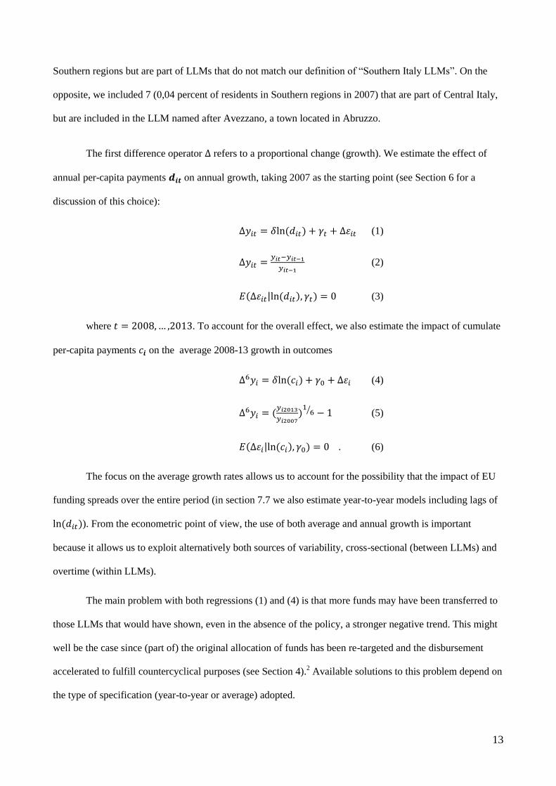
The first difference operator ∆ refers to a proportional change (growth). We estimate the effect of

annual per-capita payments 𝒅𝒊𝒕 on annual growth, taking 2007 as the starting point (see Section 6 for a

discussion of this choice):

∆𝑦𝑖𝑡 = 𝛿ln(𝑑𝑖𝑡) + 𝛾𝑡 + ∆휀𝑖𝑡 (1)

∆𝑦𝑖𝑡 =𝑦𝑖𝑡−𝑦𝑖𝑡−1

𝑦𝑖𝑡−1 (2)

𝐸(∆휀𝑖𝑡|ln(𝑑𝑖𝑡), 𝛾𝑡) = 0 (3)

where 𝑡 = 2008,… ,2013. To account for the overall effect, we also estimate the impact of cumulate

per-capita payments 𝑐𝒊 on the average 2008-13 growth in outcomes

∆6𝑦𝑖 = 𝛿ln(𝑐𝑖) + 𝛾0 + ∆휀𝑖 (4)

∆6𝑦𝑖 = (𝑦𝑖2013

𝑦𝑖2007)16⁄ − 1 (5)

𝐸(∆휀𝑖|ln(𝑐𝑖), 𝛾0) = 0 . (6)

The focus on the average growth rates allows us to account for the possibility that the impact of EU

funding spreads over the entire period (in section 7.7 we also estimate year-to-year models including lags of

ln(𝑑𝑖𝑡)). From the econometric point of view, the use of both average and annual growth is important

because it allows us to exploit alternatively both sources of variability, cross-sectional (between LLMs) and

overtime (within LLMs).

The main problem with both regressions (1) and (4) is that more funds may have been transferred to

those LLMs that would have shown, even in the absence of the policy, a stronger negative trend. This might

well be the case since (part of) the original allocation of funds has been re-targeted and the disbursement

accelerated to fulfill countercyclical purposes (see Section 4).2 Available solutions to this problem depend on

the type of specification (year-to-year or average) adopted.

14

Solutions for local time-varying omitted variables for the year-to-year specifications. By exploiting

the year-to-year variability as in equation (1), we can experiment with a number of different strategies. First

of all, we can control for LLM-specific linear time trends by adding fixed effects 𝑔𝑖, which would capture a

constant growth over the years for each LLM:

∆𝑦𝑖𝑡 = 𝛿ln(𝑑𝑖𝑡) + 𝛾𝑡 + 𝑔𝑖 + ∆휀𝑖𝑡. (7)

For equation (7) to be consistently estimated by OLS, we need a strict exogeneity condition:

𝐸[∆휀𝑖𝑠|ln(𝑑𝑖𝑡), 𝛾𝑡 , 𝑔𝑖] = 0∀𝑠, 𝑡. (8)

Shocks ∆휀𝑖𝑡 must be, conditional on time and LLM effects 𝛾𝑡 and 𝑔𝑖, uncorrelated with payments in

all time periods. This condition means that current payments should be unrelated not only with current

shocks on the local economy, but also with past and future shocks. The latter scenario is not unreasonable: it

is likely that areas where the recession was stronger felt have been able to attract more payments later. To

check whether strict exogeneity holds with our data, we run the test suggested by Wooldridge (2010, p. 325),

which amounts to adding the lead of the covariate of interest and test whether it is significant in the

regression.

The introduction of fixed effects in eq. (7) captures LLM-specific linear trends. However, there may

be quadratic or cubic trends that would require introducing additional interactions between the LLM fixed

effects and higher order time trends in the regression. This is not feasible given the short length of our data.

We exploit a different strategy, based on a set of time-invariant covariates 𝑓𝑖′. We introduce them in a year-

to-year regression and we also interact them with a linear time trend t and its square. Given that the

regression is already in first difference, this allows for linear, quadratic and cubic trends that depend on these

pre-determined variables:

∆𝑦𝑖𝑡 = 𝛿ln(𝑑𝑖𝑡) + 𝛾𝑡 + 𝑓𝑖′𝜔1 + 𝑡 × 𝑓𝑖

′𝜔2 + 𝑡2 × 𝑓𝑖′𝜔3 + ∆휀𝑖𝑡. (9)

In this case, the necessary exogeneity condition is:

𝐸(∆휀𝑖𝑡|ln(𝑑𝑖𝑡), 𝛾𝑡 , 𝑓𝑖′, 𝑡) = 0. (10)

Condition (10) differs from the one required for FE estimation. On the one hand, it allows for higher

order time trends (although in a simplified way) and it does not require strict exogeneity (only the error ∆휀𝑖𝑡

15

at time t has to be uncorrelated with payments at time t). On the other hand, it requires covariates included in

𝑓𝑖′ to be good proxies of the unobservable, so that the OLS coefficient on ln(𝑑𝑖𝑡) is a consistent estimator for

the true effect of the payments.

The vector 𝑓𝑖′ includes an extensive set of local variables, which are time-invariant: employment,

unemployment and activity rates in 2004, 2005, 2006 and 2007; (log of) the outcomes (employment,

population and house prices) in 2004, 2005, 2006 and 2007; the growth of the outcomes over 2004-07; the

total surface (in kmq), population density in 2007, average altitude, the fraction of the surface composed of

mountain municipalities and that referring to municipalities located on the cost, total number of houses per

capita (census 2001 on population 2007) and total number of empty houses per capita (census 2001 on

population 2007). In order to account for differential cyclical trends, we also control for sector composition,

by including the 2007 share of private workers in construction, trade services, and other services

(considering manufacturing as the excluded category).3 Finally, we also add the logarithm (and its square) of

the public funds that were allocated at the beginning of the programming period. This variable captures

additional pre-treatment heterogeneity, as higher allocations reflect deeper underperformances. Furthermore,

conditioning on it, we are able to capture the effect of actual spending given the theoretically available funds.

This is an interesting quantity, given that most of the recent policy debate was focused on the ability of using

the most of the available funds (see, also, section 7.5).

The strategy of including LLM characteristics interacted with time trends, as argued by Belloni et al

(2014), implies adding a very long set of covariates, which may hinder the precision of the estimators and

create problems for standard inference. The authors suggest the selection of a smaller set of variables using a

“double selection method”. Instead of assuming that one needs to control for the entire list of variables

(𝑓𝑖′, 𝑡 × 𝑓𝑖

′, 𝑡2 × 𝑓𝑖′), they assume that there is a smaller set of covariates such that, once controlling for

them, ln(𝑑𝑖𝑡 ) can be considered exogenous. The problem is that this subset is a priori unknown. The

standard procedure would be to consider only those variables that the researcher or the literature consider

more relevant. Differently, Belloni et al (2014) propose to select them by using a Least Absolute Shrinkage

and Selection Operator (LASSO), which minimizes the sum of squared residuals and an additional penalty

16

parameter that aims to reduce the overall size of the model. We defer to their paper for details about the

operator.4 The selection must be conducted on the two reduced forms

∆𝑦𝑖𝑡 = 𝛽𝑡𝑦+ 𝑓𝑖

′𝛽1𝑦+ 𝑡 × 𝑓𝑖

′𝛽2𝑦+ 𝑡2 × 𝑓𝑖

′𝛽3𝑦+ ∆𝑣𝑖𝑡

𝑦 (11)

ln(𝑑𝑖𝑡) = 𝛽𝑡𝑑 + 𝑓𝑖

′𝛽1𝑑 + 𝑡 × 𝑓𝑖

′𝛽2𝑑 + 𝑡2 × 𝑓𝑖

′𝛽3𝑑 + ∆𝑣𝑖𝑡

𝑑 (12)

and the final set of variables should be the union of those selected in (11) and (12). The reason is that

the selection aims to maximize the predictive power of the covariates, which is captured by the reduced

forms rather than by the equation of interest (9).

Solutions for local time-varying omitted variables for the average growth specifications. In eq. (4) it

is not possible to introduce LLM fixed-effects. We can therefore only add the vector of LLM-specific time-

invariant variables 𝑓𝑖′. Given that the regression is in first-differences, introducing these covariates allows for

counterfactual linear time trends that depends on pre-determined differences in these variables:

∆6𝑦𝑖 = 𝛿ln(𝑐𝑖) + 𝛾0 + 𝑓𝑖′𝜔 + ∆휀𝑖. (13)

For OLS to consistently estimate the true effect of cumulate payments, we need payments and

shocks ∆휀𝑖𝑡 to be uncorrelated given the LLM characteristics included in 𝑓𝑖′. Additionally, we also

implement the Belloni et al (2014) procedure to estimate eq. (13).

6. Data and descriptive statistics

The information on payments and allocations comes from the OpenCoesione website.5 It collects all the

information relative to projects at least partially funded by EU Structural Funds. The variable on payments

not only include the money coming from the European funds, but also the co-financing from the Italian

Government (or local authorities) and, in some cases, from the private sector. Importantly, the data provides

geo-referenced information about the targeted places. Although the majority of the projects (around 97

percent) take place at the level of municipalities, in some cases they refer to the higher administrative levels

of provinces or regions.6 In these cases, we re-allocated the spending to the municipalities on the basis of the

2007 population. Projects at the national level have been excluded. Given that we use geographical variation

as source of heterogeneity, they would be of no help in estimating the effect. Anyway, at the end of 2013 the

17

cumulate payments relative to projects at the national level amounted to only 2.3 percent of those relative to

projects at the sub-national level, that we use in the analysis.

In the cases in which national funds were used for projects funded also through EU Structural Funds,

the relative money (co-financing) is already included in our variable. There are nevertheless some projects

that are only funded by national sources (in particular the “Fondo per lo Sviluppo e la Coesione”). Their role

seems to be limited. For Southern Italy the cumulate payments over 2007-13 relative to national funds only

amounted to 0.6 billion euro, against a total of 19.4 billion euro relative to projects funded at least partially

by EU Funds. We decide not to include expenditures only financed by national sources in our main

regressions, also because they follow procedures different from the ones where EU money is at stake, but we

conducted a robustness check by adding them (see: para. 7.6). All variables relative to payments are

expressed in per-capita terms, using only population in 2007 as denominator.

In the regressions for annual growth we focus only on changes and transfers over the period 2008-13,

taking year 2007 at the starting point. Although some payment were also made during that year, their impact

is likely to be negligible: with regard to Southern LLMs, only 400 million were spent in 2007, which is 1.7

percent of the total expenditure over the entire period.

Employment figures come from the Istat Labor Force Survey, while the local population is obtained

from Istat Intercensus demographic balance reconstruction. House prices per sqm come from the

Osservatorio Immobiliare. Data were aggregated at the municipality level with the procedure described in

Cannari and Faiella (2008). Given that they are released every semester, we took a simple average over the

whole year. In order to aggregate them at the LLM level, we use the 2007 local population as a weight.

We did not make substantial alterations to the original data. We only censored the annual changes in

house prices at the 1st and 99

th percentile of the overall pooled distribution, because there were some relevant

outliers. In some LLMs in few years the annual payments were zero or less than one euro per-capita, and

they could also be negative in the case of reimbursement of previous payments relative to projects that were

stopped. These are overall very few cases: the LLM-year observations with payments amounting to less than

one euro per-capita were less than one percent in the total pooled sample and around 3 percent in 2008, and

18

there was only one case with a small per-capita negative payment. We simply imposed the logarithm to be

zero in those years. Log cumulate payments are positive in all LLMs.

[Figure 1 approximately here]

Figure 1 shows the trends in the outcomes over the entire period in the Southern Italy. Employment

decreases significantly, by approximately 10 percent. Population remains approximately constant, with a

small smooth increase. House prices initially increase in 2008, they do not decrease much during the initial

part of the crisis while they decline by around 5 percent during the last two years. Payments relative to

projects financed by EU Structural Funds appear to be countercyclical. They are negligible in 2007, they

start to be economically significant in 2008 and then they increase in 2009-10. In 2011 we observe a

significant increase, up to 200 euro per capita, which follows the actions taken by the Italian government to

speed-up the spending and re-focusing the programs (see Section 4). The increase in payments is made clear

in Figure 2, which shows the distribution of payments across LLMs by year. The amount of transfers

remained at the higher level during 2012 and 2013. The variability over time and across areas is quite

substantial. Given that in some estimates we introduce LLM fixed effects, it is also important to discuss the

size of variability within single local areas. In the overall sample, the within LLMs variance accounts for 44

percent of the total variance (after removing year fixed effects). The fraction is still very similar (40 percent)

if we exclude the first year, when payments were lower. It remains quite high even if we consider single

couple of years (around 15-20 percent).

[Figure 2 approximately here]

Figure 3 displays the geographical pattern of the cumulate per-capita payments over 2007-13. The

heterogeneity is quite substantial, also between LLMs located next to each other. Puglia (South-East) and

Calabria (the last part of mainland before Sicily), both part of the “Convergence” target, are characterized by

19

a stronger intensity of per-capita payments in most of their LLMs. The other two “Convergence” regions,

Campania (in the mainland on the West coast) and Sicily received substantial amount of funding, but they

are more concentrated in specific LLMs (e.g. the area of Naples in Campania). Sardinia, despite being not

part of the core “Converge” regions, managed to spend a large fraction of it. The other areas are less covered

by transfers, in particular the region of Abruzzo, located at the top of the map (in the mainland), although

some local labor markets still received significant amounts of payments.

[Figure 3 approximately here]

Figure 4 displays the scatterplot and raw correlation between growth in output and the logarithm of

per-capita payments. Growth rates have been de-trended by removing averages across all LLMs, to account

for the overall trend that would induce a strong negative correlation between annual changes in employment

and cumulate payments. Annual growth in outcomes does not display any significant relation with payments:

basically, linear fits are flat and the scatterplot does not highlight any particular relation (nor sensible

outliers). Average growth seems to be negatively correlated with cumulate per-capita payments over 2007-

13, while the relations with population and house prices are not statistically significant (though respectively

positive and negative).

Additional descriptive statistics on variables of interest are reported in the Additional file 1.

[Figure 4 approximately here]

7. Results

7.1 Main results

Table 1 shows simple regressions of the growth in the outcomes over the logarithm of the flow of per-capita

payments. The annual growth rates (Columns 1, 2, and 3) display no significant correlation, with negligible

20

coefficients from the economic perspective. Differently, in Column 4, where we consider the average

outcome growth, a 10 percent increase in per-capita cumulate payments (equivalent to approximately 76 euro

if evaluated at the average among LLMs) is associated with a 0.027 percent decrease in employment. This

correlation is in line with the possibility that funds have been directed towards those areas that have been hit

more strongly by the crisis. Population and house prices (specifications 5 and 6) do not show any association

with cumulate funds over the entire period.

[Table 1 approximately here]

Table 2 shows the regression results relative to annual growth in the outcomes (the variable of

interest is the log of annual per-capita flow of payments). For each outcome, we start by introducing FE to

account for linear trends. Then we add both 𝑓𝑖′ and a full set of interactions with t and t

2, to account for

higher order time trends. Finally, we select only a subset of these variables by using the “double selection”

method of Belloni et al (2014). There seems to be no evidence of an effect of the EU funding on employment

(Columns 1, 2, and 3). FE estimates seem to uncover an effect on population (Column 4) and house prices

(Column 7), but they disappear when we introduce covariates interacted with time trends (Columns 5 and 8,

respectively). The absence of any effect is confirmed by focusing only on the subset of selected covariates,

which are reported (Columns 6 and 9). It is important to highlight that the “double selection” keeps some

interactions with the time trend only for the house price regression, suggesting that heterogeneous time

trends are particularly important for this outcome. With regard to FE estimates, the strict exogeneity test does

not suggest any particular problem, as we fail to reject the null that the lead of annual per capita payments is

not significant when added to the regression.

[Table 2 approximately here]

21

Table 3 displays the results from regressions for the average growth on the log of cumulate per-

capita payments. For each outcome we show specifications that alternatively include the full set of pre-

determined variables 𝑓𝑖′, to account for potentially different trends during the recession, and only the subset

of covariates selected using Belloni et al (2014) “double selection” strategy. As for employment (Columns 1

and 2), we find a coefficient on (log) cumulative per-capita payments that is very small and not statistically

significant. The negative effect found without controlling for time-varying proxies (Table 1, Column 4)

disappears. However, the absence of an effect on population (Columns 3 and 4) is confirmed. Differently

from Table 1, Column 6, the inclusion of covariates (Column 5 and 6) seems to uncover a negative effect on

house prices.

[Table 3 approximately here]

We also experimented by restricting the analysis to those regions belonging to the “Convergence”

objective (Calabria, Campania, Puglia and Sicily), which are the most disadvantaged areas where the bulk of

the available funding is allocated.7 Results (available upon request) for average growth and cumulate per-

capita payments are similar to those presented in Table 3, apart from a negative, but statistically significant

only at the 10 percent level, coefficient in the employment regression. Regressions for annual growth

confirm the main findings from Table 2, with all the coefficients neither statistically, nor economically

significant.

One concern is that, in 2007-08, the EU funding referring to the previous (2000-06) programming

period have also been disbursed because of the n+2 rule (according to which the allocated money should be

spent within two years from the budgeting). Disbursements referring to the 2000-06 programming period are

not registered in OpenCoesione. Therefore, failing to account for these financing might impair our ability to

detect an effect for the 2007-14 funding, as we have two years in which payments overlap. To account for

this, we shorten our estimation window by excluding the growth in years 2008 and 2009. Results (available

upon request) referring to this period are very similar to those depicted in Table 2 and Table 3. The main

exception refers to a statistically significant and positive effect on employment in the year-to-year

22

specifications only, with an economic magnitude, however, very close to zero. This effect is similar to the

small positive effects in 2010-11 and 2011-12 that we find when we focus on single couples of years (see

section 7.2) and when we include lags of the explanatory variable (which forces us to exclude the first two

years, see section 7.8).

Even if there is no evidence of significant effects on the average, funds might have attenuated the

impact of the recession on the most vulnerable LLMs. In this case, we expect that payments had an effect on

the lowest percentiles of the distribution of growth rates in the outcomes. We run quantile regressions for the

25th and 75

th percentiles of the distribution, both without any covariates and with those that were retained

after “double selection”. Results are in line with those referring to the average and discussed in the text.

Finally, the choice of outcomes may be debatable. Private employment can be affected more by these

transfers. Similarly, population mobility is typically stronger for younger individuals. We also estimated the

main regressions (Tables 1-3) using as outcome the growth in the private employment in plants located in the

area, from the Istat Statistical Archive on Active Enterprises (an annual census of the private sector). Data

are currently available only up to the year 2012. Results for the average 2007-2012 growth show no effect of

the EU transfers. Estimates for annual growth are statistically significant, but only when we include the long

list of covariates, and they are anyway small in economic terms: around 0.07 percent increase in employment

with a 10 percent increase in per capita payments (similar to other results found for specific years; see

Section 7.2). We also re-estimated the main regressions using population between 25 and 34 years of age.

The empirical relation turns out to be negative, but never larger (across the different methods) than a 0.10

percent decrease with a 10 percent increase in per capita payments. Similar results, negative but smaller in

size, hold for the age classes 25-44 and 15-64.

7.2 Did the 2011 “Piano di Azione e Coesione” have any effect?

As explained in Section 4, in 2011 a number of actions were taken to ensure faster spending and a re-

focusing of the existent programs towards counter-cyclical aims. To inspect whether these actions had any

impulse on the effectiveness of funds, we replicated the regressions for annual growth by selecting couples

of annual growth rates (to have specifications that still allow us to include LLM fixed-effects).

23

With respect to employment (Table 4), the OLS results (first row) show small effects hardly

statistically significant. The FE results (second row) uncover a stronger and statistically significant effect in

2012-13, and a positive one in 2011-12, but not statistically significant. When we use (third row) fixed

covariates and their interaction with the time trend (captured by a second year dummy specific to each

subsample) we find a positive effect in 2010-11 and 2011-12, around 0.07 percent increase in employment

with a 10 percent increase in per capita payments. In this specification, payments seemed to have had a

negative effect on employment in 2008-09. The estimates obtained by using the Belloni et al (2014) selection

procedure (fourth row) are very similar to those obtained with the full set of 𝑓𝑖′ variables (the tables with the

estimates for the covariates are available in the Additional file 1). The estimated impact on employment

between 2010 and 2012 is not strong, but not negligible. In those years, the average per-capita payment

across the LLMs was 143 euro, with an average population of 63 thousand and an average total employment

of 19 thousand. This implies that an increase by 10 percent in the expenditure for the average LLM would

have increased its employment by approximately 13 units. Calculating the total increase in expenditure at the

average population (14.3 times 63 thousand), the cost per additional unit of employment would have been

around 68 thousand euro. The variability of per capita payments was actually quite high in those years, so it

is interesting to evaluate the effect of one standard deviation increase in the per capita payments

(approximately 100 euro, around 70 percent of the average). This would imply an increase in employment by

around 0.37 percent, which is 70 units if evaluated at the average.8 Overall, the acceleration/re-targeting of

the payments that started in 2011 seemed to have caused a modest rise in employment (which however loses

momentum starting from 2012).

[Table 4 approximately here]

If we focus on population (Table 5), there is no difference with our previous results pointing to an

overall ineffectiveness. OLS uncover some relations, but all other estimates are neither statistically, nor

economically significant. With respect to house prices (Table 6), results seem to suggest a positive effect in

2009-10 and a negative one (but statistically significant only at the 10 percent level) in 2012-13. The effect

24

in 2009-10 is recovered when we use only selected covariates, but it actually disappears (without a decrease

in the precision of the estimates) when we include the full set of covariates and interactions with the time

trend.9

[Tables 5 and 6 approximately here]

7.3 Is there any difference according to the type of programs?

Projects funded by EU Structural Funds are heterogeneous. Broadly speaking, they refer to four categories:

(i) payments for the purchase of goods and services; (ii) incentives for firms and workers; (iii) payments for

infrastructural projects; (iv) other expenditures (purchase of stocks or other capital transfers). For the first

category, during each year between 2008 and 2013 there were positive payments in all LLMs, although 9.5

percent of the LLMs had payments smaller than one euro per-capita in 2008. Payments related to incentives

were 0 only in 4.3 percent of the LLM-year observations (concentrated in 2008, where they represented the

24.3 percent), with an additional 3.2 percent smaller than one euro per-capita. Payments for infrastructures

were 0 in 6.9 percent of the cases, while they were negative (due to reimbursements relative to projects that

had been stopped) only for 1.1 percent of the observations. An additional 9.9 percent were smaller than one

euro per-capita. In all these cases we impose the log to be equal to zero. We ignore the last category (other

expenditures) because it amounted to 2.8 percent of total cumulate payments in 2013, with the majority of

LLM-year observations equal to 0.

In Table 7 we estimate the impact of the different kinds of expenditures, by replicating the year-to-

year specifications of Table 2. Fixed-effect estimates suggest a small but positive effect of purchase of goods

and services and incentives on employment (Column 1). For the payments relative to the purchase of goods

and services there is evidence that the strict exogeneity condition required for fixed effects to be consistent is

violated. Nevertheless, positive though smaller impacts are uncovered also through the estimation that uses

fixed time covariates and interactions with the time trend (Columns 2 and 3). On the other hand, the

payments related to infrastructural projects do not show any impact on local employment. The results

25

referring to the population and house prices growth (from Column 4 to Column 9) do not signal any

interesting pattern attributable to the different types of projects.

One possible reason for the positive effect associated with the first two categories of spending is that

their impact is more likely to be found over a short-term period. This could be particularly true for some

categories of incentives that address the crisis-induced difficulties of the firms, such as wage-

supplementation schemes and public credit guarantees. Differently, infrastructures are more likely to impact

over the longer run and therefore their effect may not be detected by our analysis. Moreover, disbursements

referred to infrastructures generally pre-date the moment in which the public goods are completed (so to

trigger economic effects on our outcomes).

Given that the logarithm of infrastructural spending displays a large mass of year-LLM observation

at zero, we also tried to run the regressions looking at the effect of the cumulate 2007-13 spending on the

average growth during the period (similarly to Table 3). In this case, all LLMs have positive payments

(larger than one euro per capita) for the three kinds of spending. For infrastructural projects, these

regressions (available on request) still display close to zero coefficients for the effects on employment and

population, and a negative one on house prices (0.05 percent decrease with a 10 percent increase in

payments). As it could be expected, in this case also the other two categories of spending show no relation

with the outcomes, probably because the short term effect on employment is hardly captured without

properly modeling the underlying annual trends. Only population appears to be slightly positive affected by

the purchase of goods and services.

[Table 7 approximately here]

7.4 Slackness in housing and labor market

A standard spatial equilibrium model, as in Kline and Moretti (2013a), suggests that the effect on population

mobility and house prices depends on the elasticity of local labor and housing supply. For instance, in a

scenario of low employment, additional labor demand generated by transfers may increase the local

26

employment rate without attracting population from other areas. Real estate prices are also more likely to

change if there is a shortage of housing supply, so that the increase in income and/or population will increase

rents. We broadly test whether the implications of the spatial equilibrium model apply in our data, by

constructing two simple indicators of labor and housing market slackness. The first is a dummy variable for

the lowest quintile of employment rate in 2007, which should capture those areas that have a larger

availability of potential labor supply. The second is an indicator for the lowest quintile of housing prices in

2007, which should capture the availability of affordable housing.

Table 8 shows the results from regressions for annual growth that also include interactions between

the flow of payments and the indicators for slackness in housing and labor market (plus the main effect of

these two variables in regressions without FE). We fail to find any evidence of a differential effect on

employment (Columns 1-3). When using fixed effects (Column 4) or “double selected” LLM characteristics

(Column 6), population seems to be negatively affected on average, but the presence of affordable housing

seems to compensate this effect (the results from controlling for the full set of 𝑓𝑖′ variables are similar but not

significant at the usual levels). The housing slackness (Columns 7-9) seems also to have a counteracting

effect on the evolution of housing prices (but statistically significant only at the 10 percent level).

Differently, the labor market slackness is associated with a positive effect of the European funds, which is a

result that does not lend credit to the implications of the spatial equilibrium model.

[Table 8 approximately here]

7.5 Faster disbursements?

A recurring argument in the Italian policy debate on Structural Funds refers to the actual capacity of

spending the available EU money. For instance, for Southern Italy, at the end of 2013, only roughly 50

percent of the resources available for the 2007-13 programming period was spent. A popular argument is that

if local authorities would have been able to spend all the available EU money then the economic

consequences of the crisis could have been less dramatic. We have already highlighted that the acceleration

of funding achieved with the “Piano di Azione and Coesione” may have had only a reduced impulse on

27

employment starting from 2011. In this Section, we study whether those LLMs that have been able to spend

the most of the allocated money have shown better performances compared with their less efficient

counterparts.

To this purpose, in Table 9 we focus on the average growth 2008-13, and replace the variable of

interest, which is taken now to be the fraction of available funds that have been spent by the end of 2013.10

The results are extremely similar to those we found in the baseline estimates of Table 3.11

It does not seem,

therefore, that those LLM who spent a larger fraction of the available funding experienced higher

effectiveness of the interventions.

[Table 9 approximately here]

7.6 Interactions with national funding

As discussed in Section 4, during 2007-13 there were also cohesion projects entirely funded by

national sources. These concurrent programs are likely not going to make a difference for the estimated

effectiveness of EU funding: they amount to 3.1 percent of the EU transfers we have considered up to now.

In any case, in Table 10 we add per-capita payments relative to nationally-funded programs in the

regressions. We focused on the average growth specification because these funds are more limited and

therefore in some years they amount to zero for the vast majority of LLMs.12

On the whole period the LLMs

with less than one euro per-capita of expenditure from these funds are 43 (13 percent; 11 LLMs have zero

payments), and we recode their logarithm to zero. Results without this correction (excluding those with zero

payments) and results for annual growth (imposing the logarithm to be zero) lead to similar conclusions and

are available on request.

Table 10 shows that the expenditure related to national sources is unrelated with all three outcomes

(apart from a marginally statistically and economically significant relation with employment found in

Column 1). It is therefore not surprising that the estimated effects of the EU funds are extremely similar to

the main estimates provided in Table 2.

28

[Table 10 approximately here]

7.7 Absorptive capacity: heterogeneity by human capital

Becker et al (2013) find that regions characterized by lower human capital and/or quality of

institutions are less able to reap the gains of European transfers, even if they manage to qualify as

“Convergence” regions and, therefore, to receive a substantial amount of financing.

With respect to the quality of institutions, we unfortunately cannot obtain good enough proxies,

given that we would need data at the municipality level in order to aggregate them by LLM. To the best of

our knowledge, only Barone and Mocetti (2011) developed an indicator of public spending efficiency at this

level, but the indicator is available only for a subsample (approximately one fifth) of municipalities for

which the required data were available. This prevents us from building a reasonably good proxy, given that

we would also have to aggregate the different municipalities included in each LLM.

Differently, the 2001 Census allows us to recover the fraction of the population aged 6 or more with

at least a high school diploma. Similarly to Becker et al (2013), we take it as deviations from the average

across Southern LLM and we add it to the regression, both linearly and interacted with the payments.13

In the

annual growth regressions, the interaction term is positive for employment and house prices, but small in

economic terms and not statistically significant. It is generally negative for population, but marginally

statistically significant (at the 10 percent level) only when we add the full set of covariates (results available

on request). The patterns are less clear in the average growth specification, but still neither statistically nor

economically significant. The aggregate results about the effect of European transfer payments does not

seem, therefore, to display a significant heterogeneity by human capital.

This is not necessarily inconsistent with Becker et al (2013). Indeed, their method allows them to

compute, for each country, the share of Objective 1 regions whose human-capital and institutional quality is

sufficient for displaying a positive effect of European transfers. For Italy, none of the regions satisfies the

criteria for displaying an effect on GDP per-capita growth. Half of them meet the required threshold for a

29

positive effect on investment, but with large statistical imprecision in the potential effect (idem, pg. 57). It is

therefore not surprising that the differences of human capital within Southern Italy are not, according to our

results, sufficient to generate a sensible heterogeneity in the effects.

7.8 Specification issues

In the year-to-year regressions we focused on the contemporary (annual) effects. However, the

impact of the payments may take some time to materialize. In Table 11 we re-estimate the regression for

annual growth including two lags of the logarithm of per-capita payments.14

In order to do this, we need to

focus only on the 2010-2013 period. In Table 11, columns (1)-(3) show a small but positive effect of the

current annual payments on employment, while no effect is found on population or prices. Crucially, lags

exhibit minor and not statistically significant coefficients on employment. The first lag seems to have a

negative and very modest effect on population and again a negative, but larger effect on house prices.

However, both estimates are imprecise and statistically significant only at the 10 percent level. Two-year

lags are neither economically nor statistically significant. All in all, taking aboard past disbursements seems

not to add significantly to the overall picture of ineffectiveness.

[Table 11 approximately here]

Finally, instead of studying the effect on growth, one may want to look at the elasticity of the level of

the outcome with respect to payments related to EU projects. In this case, we need to account at the same

time for LLM fixed effects and for heterogeneous time trend. The equivalent of the FE regression for the

annual growth in the outcomes is:

𝑦𝑖𝑡 = exp(𝛿ln(𝑑𝑖𝑡) + 𝛾𝑡 + 𝑢𝑖 + 𝑔𝑖 × 𝑡)𝜂𝑖𝑡 (14)

𝐸[𝜂𝑖𝑠|ln(𝑑𝑖𝑡), 𝛾𝑡 , 𝑢𝑖, 𝑔𝑖 × 𝑡] = 1∀𝑠, 𝑡 (15)

which can be estimated using Poisson Quasi Maximum Likelihood (PMQL, see Santos Silva and Tenreyro,

2006, for a general discussion and Ciani and Fisher, 2014, for the dif-in-dif case).15

The coefficient 𝛿 can be

interpreted as the elasticity of the outcome with respect to the per-capita payments. In line with previous

30

estimates, we can also allow for higher order heterogeneous time trends by using the interaction between

time trends and fixed time variables, and select them using Belloni et al (2014) “double selection”.16

In this

case we show only regressions with the selected variables, because Poisson regressions with the entire set do

not converge due to the large set of covariates.

Table 12 displays the results. No effect is detected for any of the outcomes, in line with the main

results.

[Table 12 approximately here]

A final concern regards the specification of the time components in the regressions for annual

growth. On the one hand, the model with LLM specific linear trends, estimated using fixed effects, may not

be sufficient. On the other, the interactions of linear and quadratic time trends with pre-determined variables

may be a poor representation of the actual dynamics. We also tried two alternative ways.17

The first involves adding, in the regressions for annual growth including fixed effects (LLM specific

linear trends, see eq. 7), interactions between the year dummies and (i) region dummies and (ii) indexes of

specialization in different sectors in 2007 (share of private workers in construction, trade services, and other

services, considering manufacturing as the excluded category). Results are very similar to the ones presented

in Table 2.

The second involves adding an explicit dynamics in the regression, by allowing current growth in the

outcomes to depend on previous growth. We estimated

∆yit = ρ∆yit−1 + δln(dit) + γt + ∆εit (16)

by instrumenting ∆yit−1 with ∆yit−2 (given that the error ∆εit is by construction correlated with the

first lag), following the traditional approach proposed by Anderson and Hsiao (1982). Results for

employment and population show that current growth depends on its lag, but the coefficient on the log of

payments is close to zero, as in the main estimates. The regression for house prices is not identified, due to a

weak first-stage.18

Finally, we could include fixed effects (LLM specific linear time trends) in eq. (16).

31

However, for it to be correctly estimated we need to take its first difference (for each variable xit, ∆2xit =

∆xit − ∆xit−1) and instrument ∆2yit−1with ∆yit−3. The third lag is necessary because ∆2εit = (εit − εit−1) −

(εit − εit−2) and therefore ∆yit−2 is correlated with it.19

Unfortunately, this specification is, empirically,

extremely demanding in terms of identification. Only the equation for population is identified, and results are

in line with those presented in the main text.20

We also tried to simply estimate this “double-difference”

regression using OLS, although, as well known, this introduces a bias. We lose one year because the

difference in payments is not defined before 2009, so results get closer to the specifications in which we keep

only more recent years. There is a small positive effect on employment (0.04 percent increase for a 10

percent increase in per-capita payments, and statistically significant only at the 10 percent level) and on

house prices (0.21 percent increase for a 10 percent increase in per-capita payments, statistically significant

at the 5 percent level). Both are likely to be driven by an incorrect specification of the time trends, as they

disappear when we include the interactions between year and region dummies, and between year and indexes

of specialization.

8. Conclusions

Our analysis suggests that EU Structural Funds disbursed in the South of Italy between 2007 and

2013 had only a limited impact on local measures for employment, population, and house prices. Modest

effects on employment only are uncovered for the acceleration/re-targeting of payment that started in 2011.

Short term effects seem to be associated with the EU money channeled through incentives and the purchase

of goods and services. A relevant upshot of our empirical investigation refers to the so called financial

execution of the budgets, an issue hotly debated in policy circles. We do not find evidence that speeding-up

disbursements would have had a more beneficial impact on the local economic outcomes that we consider. A

joint reading of two results, the one related to the 2011 “Piano di Azione e Coesione” and the one referring to

the speed of the financial execution, would suggest that the effects of the former are mostly related to the re-

focusing, rather than the acceleration per se. Overall, our findings underscore that the targets and design of

the interventions have to be reformed to increase their effectiveness.

32

It is worth mentioning, though, the two main caveats of our exercise. Firstly, our estimates are

basically diff-in-diffs estimates, where the treatment is taken to be continuous. In this set-up, and because of

the concomitant severe economic crisis, the main challenge is to reduce the role of omitted time-varying

variables. We try to accomplish this job, by controlling for an extensive list of LLM-specific traits that

should help in predicting local trends. Obviously, one cannot be ensured that all the sources of local

dynamics are successfully differentiated away, even though we control for all the local traits that should

reasonably have a role in explaining the severity of the crisis in a given local context. We also believe that

the limitations of the empirical framework we adopt should be weighed against the benefits of having timely

empirical evidence on the effectiveness of the 2007-13 EU Structural Funds. Having such evidence, while

the design of the interventions for the next programming period (2014-20) of the EU Structural Funds is

under way, should be extremely valuable for policy making.

Secondly, we focus on a single area, the South of Italy, that has been severely hit by the economic

crisis. The extent to which our results might provide lessons for other EU countries or timespan with less

dramatic economic conditions is something that is left to further inquiries. Furthermore, as we currently have

to limit our analysis to the six years of the programming period, future research projects can try to study

whether stronger effects might be found in the longer run.

Endnotes

1 The definition was built using the same algorithm previously used in 1991 (Istat, 1997). The 2001 map was

recently revised using the new method that was implemented starting with the 2011 Census (see

http://www.istat.it/en/archive/142790; last access: 30/06/2015). At the moment of writing, the data at the

local level that have been used in this paper are not available for this new definition.

2 Because of the dramatic economic crisis, we are mostly concerned with the downward bias due to time-

varying omitted at the local level. Obviously, one could also imagine that the bias goes in the other direction.

33

For instance, the most efficient local administrations could have obtained more money, as the EU programs

managed by them were executed in a faster way.

3 These variables have been included in the spirit of Bartik (1991), who calculates local shocks by interacting

the begin-of-the-period industry composition with the nation-wide changes industry-specific changes in

employment. The data were obtained from the ASIA archive, which collects the entire population of private

sector firms and plants. Unfortunately, these data are not currently available at the industry-LLM level for

2013. See Section 7.1 for the discussion of results using ASIA to build an alternative outcome variable.

4 We used the Stata program lassoShooting written by them.

5 www.opencoesione.gov.it

6 In some cases, the projects contain information about multiple geographical levels. For example, it may list

both a set of municipalities and some provinces (or an entire region). In these cases, we chose to give priority

to the information pertaining to the most disaggregated level. For instance, in the example just discussed, we

only considered the municipalities explicitly mentioned, ignoring the information on provinces or regions.

7 Another region, Basilicata, is in the phasing out phase.

8 The calculation for the growth in employment is performed as 0.007 (the coefficient on logarithm

payments) times the logarithm of 1.7 (170%). The cost per unit increase evaluated at the average would be

somewhat larger (90 thousand euro) than the one for a 10 percent increase in payments.

9 One potential concern with the procedure of sample-splitting implemented in Tables 4-6 is that some

statistically significant results are likely to be found also by chance. To address this concern, for each

estimation method we jointly test the null that the coefficients on log payments is equal to zero in all couples

of years. P-values are generally in line with the conclusions described in the text (see last columns of Tables

4-6).

10 Given that the explicative variable changes, we run again the “double selection” procedure, but the

selected covariates ended up to be the same as in Table 2.

34

11 In the baselines, however, we use the disbursements as variable of interest but we also controlled for the

allocations.

12 To avoid introducing different sources of variation in the results, we keep the same list of covariates as in

Table 2.

13 Becker et al (2013) used the fraction of workers holding at least a high school diploma. Unfortunately,

ISTAT does not release data on workers’ education at the LLM level, neither from the 2001 Census, nor

from the annual Labour Force Survey.

14 Payments may also arrive after the projects have been carried out. In this case, we may want to study the

effect of the first lead of the main explicative variables. Note, however, that we have already tested the

significance of a lead as part of the test for strict exogeneity in the FE equations and it was never significant.

15 The alternative is to log-linearize the model and use OLS. However, this method, although standard, is

biased under heteroskedasticity, which instead does not affect the consistency of PQMLE (Santos Silva and

Tenreyro, 2006; Ciani and Fisher, 2014).

16 Formally, the equation becomes (being in levels, we keep the LLM fixed effects):

𝑦𝑖𝑡 = exp(𝛿ln(𝑑𝑖𝑡) + 𝛾𝑡 + 𝑢𝑖 + 𝑡 × 𝑓𝑖′𝜑1 + 𝑡2 × 𝑓𝑖

′𝜑2 + 𝑡3 × 𝑓𝑖′𝜑3)𝜂𝑖𝑡

𝐸(𝜂𝑖𝑡|ln(𝑑𝑖𝑡), 𝛾𝑡 , 𝑓𝑖′, 𝑡) = 1.

For the selection of covariates, although there are methods for the non-linear cases, here we simplify by log-

linearizing the two reduced forms (this is potentially biased, see footnote 15).

17 We thank Paolo Sestito for suggesting both

18 Similar results are obtained by using ln(𝑦𝑖𝑡−2) as instrument.

19 It must be said that this definition of ∆2휀𝑖𝑡 is not exact, because the original equation has been taken as

proportional variations and not as simple differences. The point is nevertheless the same.

20 We also tried different specifications with additional lags of levels and differences.

35

References

Accetturo A, de Blasio G (2012) Policies for Local Development: an Evaluation of Italy’s “Patti

Territoriali”, Reg Sci Urban Econ, 42(1-2): 15-26. doi:10.1016/j.regsciurbeco.2011.04.005

Accetturo A, de Blasio G, Ricci L (2014) A Tale of Unwanted Outcome: Transfers and the Local

Endowments of Trust and Cooperation, J Econ Behav Organ, 102: 74-89. doi:10.1016/j.jebo.2014.03.015

Aiello F, Pupo V (2012) Structural fund and the economic divide in Italy, Journal of Policy

Modeling 34: 403-418. doi:10.1016/j.jpolmod.2011.10.006

Anderson TW, Hsiao C (1982) Formulation and estimation of dynamic models using panel data,

Journal of Econometrics 18: 47–82

Andini M, de Blasio G (2014) Local Development that Money Can’t Buy: Italy’s Contratti di

Programma, Journal of Economic Geography first published online November 4, 2014. doi:

10.1093/jeg/lbu048

Barca F, McCann P, Rodríguez-Pose A (2012) The case for regional development intervention:

Place-based versus place-neutral approaches, J Regional Sci, 52(1): 134-152. doi: 10.1111/j.1467-

9787.2011.00756.x

Bartik T J (1991) Who Benefits From State and Local Economic Development Policies. W.E.

Upjohn Institute for Employment Research: Kalamazoo, Mich.

Barone G, Mocetti S (2011) Tax morale and public spending inefficiency, Int Tax Public Finance

18(6): 724-749. doi: 10.1007/s10797-011-9174-z

Belloni A, Chernozhukov V, Hansen C. (2014) High-Dimensional Methods and Inference on

Structural and Treatment Effects, J Econ Perspect, 28(2): 29-50. doi: 10.1257/jep.28.2.29

Becker SO, Egger PH, von Ehrlich M (2010) Going NUTS: The effect of EU Structural Funds on

regional performance, J Public Econ, 94(9-10): 578-590. doi:10.1016/j.jpubeco.2010.06.006

Becker SO, Egger PH, von Ehrlich M (2012) Too much of a good thing? On the growth effects of

the EU’s regional policy, Eur Econ Rev, 56(4): 648-668. doi:10.1016/j.euroecorev.2012.03.001

36

Becker SO, Egger PH, von Ehrilich M (2013) Absorptive Capacity and the Growth and Investment

Effects of Regional Transfers: A Regression Discontinuity Design with Heterogeneous Treatment Effects,

AEJ: Policy 5(4): 29-77. doi: 10.1257/pol.5.4.29

Besley T (2004) Paying politicians: theory and evidence, J Eur Econ Assoc 2: 193–215. doi:

10.1162/154247604323067925

Boldrin M, Canova F (2001) Inequality and convergence in Europe’s regions: reconsidering

European regional policies, Econ Policy, 16(32): 205-253

Bronzini R, de Blasio G (2006) Evaluating the Impact of Investment Incentives: The Case of Italy’s

Law 488/1992, J Urban Econ, 60: 327-349

Cannari A, Faiella I (2008) House prices and housing wealth in Italy, in Banca d’Italia (eds),

Household Wealth in Italy, Rome, Italy

Ciani E, Fisher P (2014) Dif-in-dif estimators for multiplicative treatment effects, Temi di

discussione (Economic working papers) 985, Bank of Italy

European Commission (2008a), Communication from the Commission to the European Council – A

European Economic Recovery Plan, Brussels, 26/11/2008

European Commission (2008b), Road to recovery: the Cohesion package – Questions and Answers

on the contribution of Cohesion Policy to the European Economic Recovery Plan, MEMO/08/740

Giua M (2014) Spatial discontinuity for the impact assessment of the EU Regional Policy. The case

of Italian Objective 1 regions, mimeo, University Roma Tre Department of Economics working paper n. 197

Glaeser E (2008), Cities, agglomeration and spatial equilibrium, Oxford University Press, Oxford.

Glaeser E, Gottlieb JD (2008) The Economics of Place-Making Policies, Brookings Pap Eco Ac

39(1): 155-253. doi: 10.1353/eca.0.0005

Istat (1997) I sistemi locali del lavoro 1991, Argomenti n. 10, Istituto Nazionale di Statistica, Rome,

Italy.

37

Kline P, Moretti E (2013a) People, Places and Public Policy: Some Simple Welfare Economics of

Local Economic Development Programs, NBER Working Paper 19659

Kline P, Moretti E (2013b) Place Based Policies with Unemployment, NBER Working Paper 18758

Krueger A (1974) The political economy of the rent-seeking society. Am Econ Rev 64 (3): 291–303.

Neumark D, Simpson H (2014) Place-Based Policies, NBER Working Paper 20049

Pellegrini G, Terribile F, Tarola O, Muccigrosso T, Busillo F (2013) Measuring the effect of

European Regional Policy on Economic Growth: a Regression Discontinuity Approach, Pap Reg Sci, 92(1):

217-233. doi: 10.1111/j.1435-5957.2012.00459.x

Sala-i-Martin X (1996) Regional Cohesion: Evidence and Theories of Regional Growth and

Convergence, Eur Econ Rev, XL: 1325–1352.

Santos Silva JMC, Tenreyro S (2006) The Log of Gravity, Rev Econ Stat, 88(4): 641-658. doi:

10.1162/rest.88.4.641

Signorini LF, Visco I (2002) L’economia italiana, Il Mulino, Bologna

Wooldridge J (2010) Econometric Analysis of Cross Section and Panel Data, 2nd

edition, MIT Press

38

Illustrations and figures

Figure 1 Annual European Structural Funds payments (euro/capita, right axis) and trends in

employment, population and house prices (index 2007=100, left axis), 2007-2013, Southern Italy

Notes: Annual payments are per-capita, calculated divided total payments to Southern Italy by total

Southern population in 2007. Employment data are from Labor Force Surveys, house price per sqm from

Osservatorio Immobiliare (aggregated at the area level by weighting with 2007 population), population from

Istat intercensus reconstruction, annual payments from Opencoesione website.

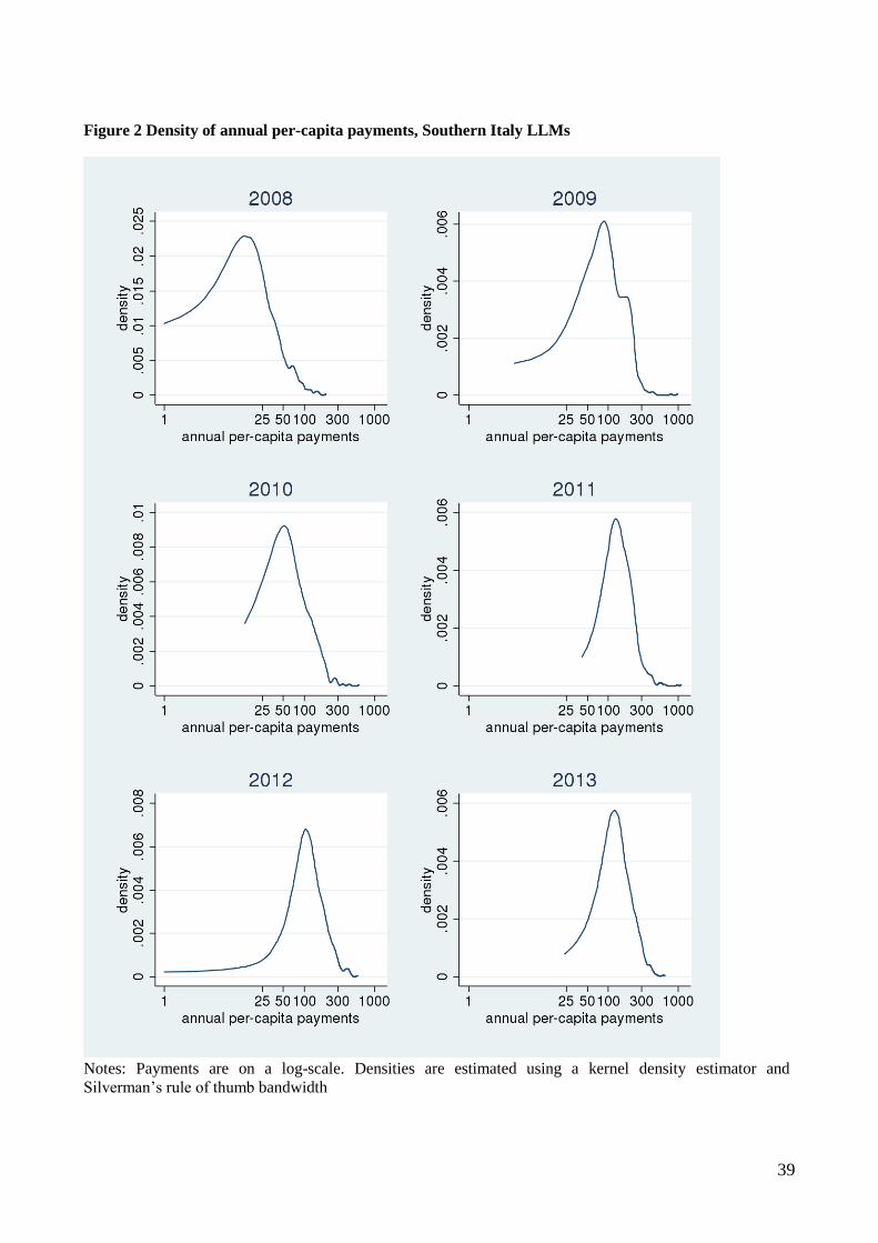
39

Figure 2 Density of annual per-capita payments, Southern Italy LLMs

Notes: Payments are on a log-scale. Densities are estimated using a kernel density estimator and

Silverman’s rule of thumb bandwidth

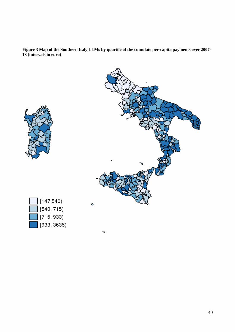
40

Figure 3 Map of the Southern Italy LLMs by quartile of the cumulate per-capita payments over 2007-

13 (intervals in euro)

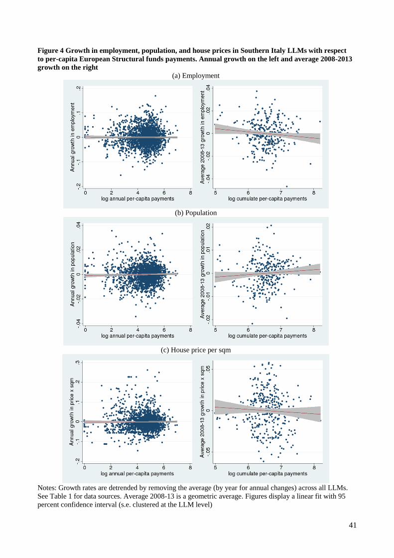
41

Figure 4 Growth in employment, population, and house prices in Southern Italy LLMs with respect

to per-capita European Structural funds payments. Annual growth on the left and average 2008-2013

growth on the right

(a) Employment

(b) Population

(c) House price per sqm

Notes: Growth rates are detrended by removing the average (by year for annual changes) across all LLMs.

See Table 1 for data sources. Average 2008-13 is a geometric average. Figures display a linear fit with 95

percent confidence interval (s.e. clustered at the LLM level)

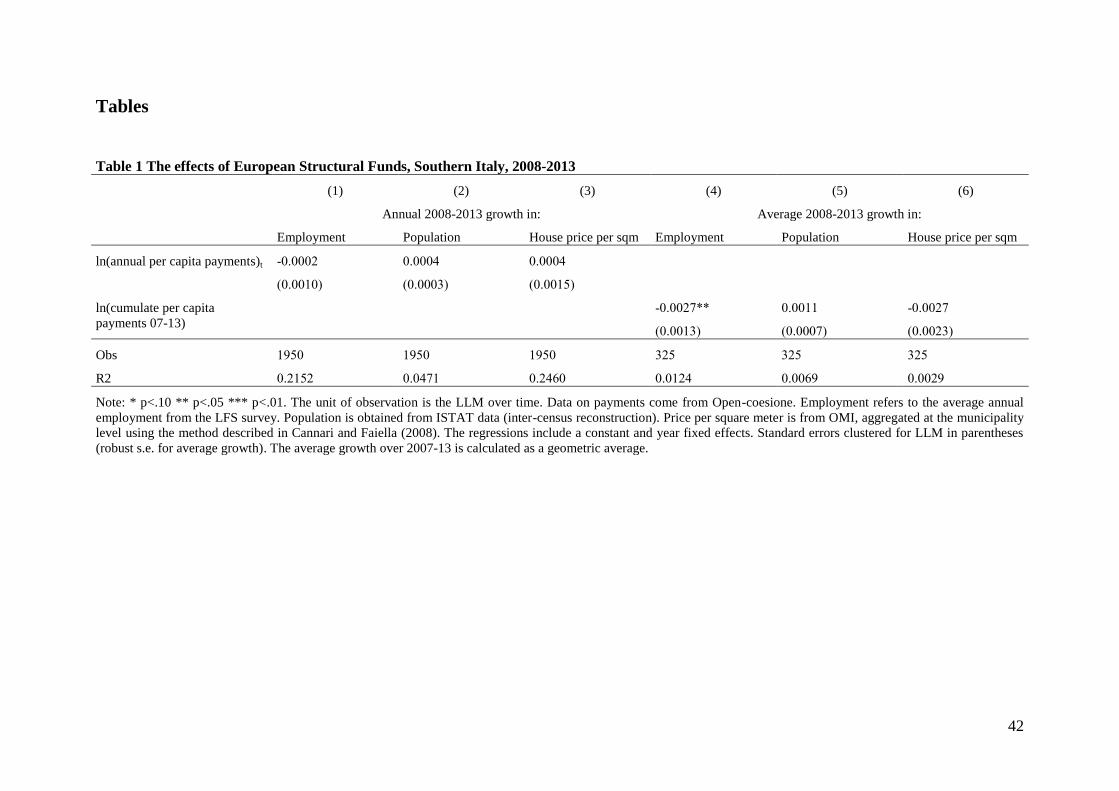
42

Tables

Table 1 The effects of European Structural Funds, Southern Italy, 2008-2013

(1) (2) (3) (4) (5) (6)

Annual 2008-2013 growth in: Average 2008-2013 growth in:

Employment Population House price per sqm Employment Population House price per sqm

ln(annual per capita payments)t -0.0002 0.0004 0.0004

(0.0010) (0.0003) (0.0015)

ln(cumulate per capita

payments 07-13)

-0.0027** 0.0011 -0.0027

(0.0013) (0.0007) (0.0023)

Obs 1950 1950 1950 325 325 325

R2 0.2152 0.0471 0.2460 0.0124 0.0069 0.0029

Note: * p<.10 ** p<.05 *** p<.01. The unit of observation is the LLM over time. Data on payments come from Open-coesione. Employment refers to the average annual

employment from the LFS survey. Population is obtained from ISTAT data (inter-census reconstruction). Price per square meter is from OMI, aggregated at the municipality

level using the method described in Cannari and Faiella (2008). The regressions include a constant and year fixed effects. Standard errors clustered for LLM in parentheses

(robust s.e. for average growth). The average growth over 2007-13 is calculated as a geometric average.

43

Table 2 The effects of European Structural Funds on annual growth, controlling for LLM time invariant characteristics and differential time trends

Annual 2008-13 growth in: (1) (2) (3) (4) (5) (6) (7) (8) (9)

Employment Population House price per sqm

ln(annual per capita

payments)t

0.0028 0.0010 0.0014 -0.0004** -0.0000 -0.0003 0.0063** 0.0012 0.0029

(0.0017) (0.0017) (0.0014) (0.0002) (0.0002) (0.0002) (0.0025) (0.0020) (0.0021)

Controls selected by the double selection procedure:

ln(allocated per capita

funds)

-0.0756 -0.0034** -0.0052 0.0002 0.2453*** 0.0034

(0.0879) (0.0014) (0.0116) (0.0003) (0.0929) (0.0026)

fraction of surface

composed of municipalities

on the coast

-0.0015 -0.0004 0.0010* 0.0183

(0.0152) (0.0019) (0.0006) (0.0172)

fraction of surface

composed of municipalities

in a mountain area

-0.0084 0.00132 0.0300* 0.0055*

(0.0131) (0.0017) (0.0157) (0.0031)

unemployment rate2006 -7.5712** -0.0243 -5.4767* -0.1442***

(3.5826) (0.3705) (3.2750) (0.0524)

ln(employment)2006 2.0891 0.1027 0.0008*** 1.0234

(1.2758) (0.2218) (0.0002) (1.4014)

population growth 2004-07 -1.7737 0.2652*** 0.6807 0.2124*** 1.2108

(2.7249) (0.0278) (0.4949) (0.0109) (4.6594)

house price growth 2004-07 0.0881 -0.0170 0.0022** -0.6140***

(0.1615) (0.0201) (0.0010) (0.1818)

share trade services workers

2007

-0.0980 -0.0002 0.0084*** 0.1629**

(0.0658) (0.0081) (0.0026) (0.0636)

housing units pc × time2 -0.0124 0.0016 -0.0009 0.0008***

(0.0212) (0.0030) (0.0198) (0.0002)

Continues next page

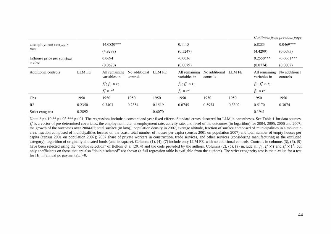
44

Continues from previous page

unemployment rate2006 ×

time

14.0820*** 0.1115 6.8283 0.0469***

(4.9298) (0.5247) (4.4299) (0.0095)

ln(house price per sqm)2006

× time

0.0694 -0.0036 0.2550*** -0.0061***

(0.0620) (0.0079) (0.0774) (0.0007)

Additional controls LLM FE All remaining

variables in

𝑓𝑖′; 𝑓𝑖

′ × 𝑡;

𝑓𝑖′ × 𝑡2

No additional

controls

LLM FE All remaining

variables in

𝑓𝑖′; 𝑓𝑖

′ × 𝑡;

𝑓𝑖′ × 𝑡2

No additional

controls

LLM FE All remaining

variables in

𝑓𝑖′; 𝑓𝑖

′ × 𝑡;

𝑓𝑖′ × 𝑡2

No additional

controls

Obs 1950 1950 1950 1950 1950 1950 1950 1950 1950

R2 0.2350 0.3403 0.2354 0.1519 0.6745 0.5934 0.3302 0.5170 0.3074

Strict exog test 0.2892 0.6070 0.1941

Note: * p<.10 ** p<.05 *** p<.01. The regressions include a constant and year fixed effects. Standard errors clustered for LLM in parentheses. See Table 1 for data sources.

𝑓𝑖′ is a vector of pre-determined covariates: the employment rate, unemployment rate, activity rate, and level of the outcomes (in logarithm) for 2004, 2005, 2006 and 2007;

the growth of the outcomes over 2004-07; total surface (in kmq), population density in 2007, average altitude, fraction of surface composed of municipalities in a mountain

area, fraction composed of municipalities located on the coast, total number of houses per capita (census 2001 on population 2007) and total number of empty houses per

capita (census 2001 on population 2007); 2007 share of private workers in construction, trade services, and other services (considering manufacturing as the excluded

category); logarithm of originally allocated funds (and its square). Columns (1), (4), (7) include only LLM FE, with no additional controls. Controls in columns (3), (6), (9)

have been selected using the “double selection” of Belloni et al (2014) and the code provided by the authors. Columns (2), (5), (8) include all 𝑓𝑖′, 𝑓𝑖

′ × 𝑡 and 𝑓𝑖′ × 𝑡2, but

only coefficients on those that are also “double selected” are shown (a full regression table is available from the authors). The strict exogeneity test is the p-value for a test

for H0: ln(annual pc payments)t+1=0.

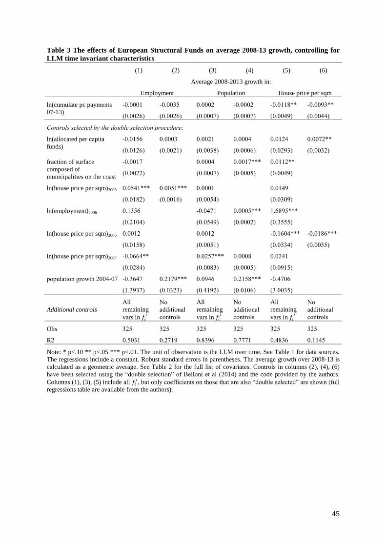
45

Table 3 The effects of European Structural Funds on average 2008-13 growth, controlling for

LLM time invariant characteristics

(1) (2) (3) (4) (5) (6)

Average 2008-2013 growth in:

Employment Population House price per sqm

ln(cumulate pc payments

07-13)

-0.0001 -0.0035 0.0002 -0.0002 -0.0118** -0.0093**

(0.0026) (0.0026) (0.0007) (0.0007) (0.0049) (0.0044)

Controls selected by the double selection procedure:

ln(allocated per capita

funds)

-0.0156 0.0003 0.0021 0.0004 0.0124 0.0072**

(0.0126) (0.0021) (0.0038) (0.0006) (0.0293) (0.0032)

fraction of surface

composed of

municipalities on the coast

-0.0017 0.0004 0.0017*** 0.0112**

(0.0022) (0.0007) (0.0005) (0.0049)

ln(house price per sqm)2005 0.0541*** 0.0051*** 0.0001 0.0149

(0.0182) (0.0016) (0.0054) (0.0309)

ln(employment)2006 0.1356 -0.0471 0.0005*** 1.6895***

(0.2104) (0.0549) (0.0002) (0.3555)

ln(house price per sqm)2006 0.0012 0.0012 -0.1604*** -0.0186***

(0.0158) (0.0051) (0.0334) (0.0035)

ln(house price per sqm)2007 -0.0664** 0.0257*** 0.0008 0.0241

(0.0284) (0.0083) (0.0005) (0.0915)

population growth 2004-07 -0.3647 0.2179*** 0.0946 0.2158*** -0.4706

(1.3937) (0.0323) (0.4192) (0.0106) (3.0035)

Additional controls

All

remaining

vars in 𝑓𝑖′

No

additional

controls

All

remaining

vars in 𝑓𝑖′

No

additional

controls

All

remaining

vars in 𝑓𝑖′

No

additional

controls

Obs 325 325 325 325 325 325

R2 0.5031 0.2719 0.8396 0.7771 0.4836 0.1145

Note: * p<.10 ** p<.05 *** p<.01. The unit of observation is the LLM over time. See Table 1 for data sources.

The regressions include a constant. Robust standard errors in parentheses. The average growth over 2008-13 is

calculated as a geometric average. See Table 2 for the full list of covariates. Controls in columns (2), (4), (6)

have been selected using the “double selection” of Belloni et al (2014) and the code provided by the authors.

Columns (1), (3), (5) include all 𝑓𝑖′, but only coefficients on those that are also “double selected” are shown (full

regressions table are available from the authors).

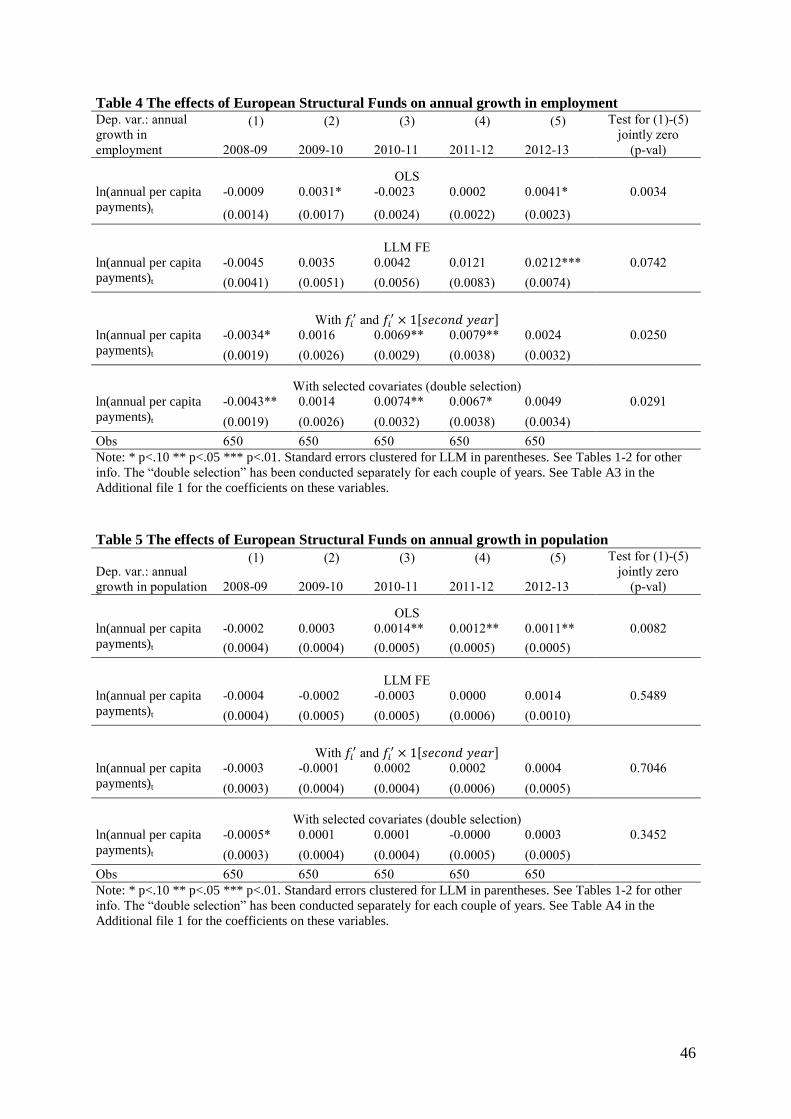
46

Table 4 The effects of European Structural Funds on annual growth in employment Dep. var.: annual

growth in

employment

(1) (2) (3) (4) (5) Test for (1)-(5)

jointly zero

(p-val) 2008-09 2009-10 2010-11 2011-12 2012-13

OLS

ln(annual per capita

payments)t

-0.0009 0.0031* -0.0023 0.0002 0.0041* 0.0034

(0.0014) (0.0017) (0.0024) (0.0022) (0.0023)

LLM FE

ln(annual per capita

payments)t

-0.0045 0.0035 0.0042 0.0121 0.0212*** 0.0742

(0.0041) (0.0051) (0.0056) (0.0083) (0.0074)

With 𝑓𝑖′ and 𝑓𝑖

′ × 1[𝑠𝑒𝑐𝑜𝑛𝑑𝑦𝑒𝑎𝑟]

ln(annual per capita

payments)t

-0.0034* 0.0016 0.0069** 0.0079** 0.0024 0.0250

(0.0019) (0.0026) (0.0029) (0.0038) (0.0032)

With selected covariates (double selection)

ln(annual per capita

payments)t

-0.0043** 0.0014 0.0074** 0.0067* 0.0049 0.0291

(0.0019) (0.0026) (0.0032) (0.0038) (0.0034)

Obs 650 650 650 650 650

Note: * p<.10 ** p<.05 *** p<.01. Standard errors clustered for LLM in parentheses. See Tables 1-2 for other

info. The “double selection” has been conducted separately for each couple of years. See Table A3 in the

Additional file 1 for the coefficients on these variables.

Table 5 The effects of European Structural Funds on annual growth in population

Dep. var.: annual

growth in population

(1) (2) (3) (4) (5) Test for (1)-(5)

jointly zero

(p-val) 2008-09 2009-10 2010-11 2011-12 2012-13

OLS

ln(annual per capita

payments)t

-0.0002 0.0003 0.0014** 0.0012** 0.0011** 0.0082

(0.0004) (0.0004) (0.0005) (0.0005) (0.0005)

LLM FE

ln(annual per capita

payments)t

-0.0004 -0.0002 -0.0003 0.0000 0.0014 0.5489

(0.0004) (0.0005) (0.0005) (0.0006) (0.0010)

With 𝑓𝑖′ and 𝑓𝑖

′ × 1[𝑠𝑒𝑐𝑜𝑛𝑑𝑦𝑒𝑎𝑟]

ln(annual per capita

payments)t

-0.0003 -0.0001 0.0002 0.0002 0.0004 0.7046

(0.0003) (0.0004) (0.0004) (0.0006) (0.0005)

With selected covariates (double selection)

ln(annual per capita

payments)t

-0.0005* 0.0001 0.0001 -0.0000 0.0003 0.3452

(0.0003) (0.0004) (0.0004) (0.0005) (0.0005)

Obs 650 650 650 650 650

Note: * p<.10 ** p<.05 *** p<.01. Standard errors clustered for LLM in parentheses. See Tables 1-2 for other

info. The “double selection” has been conducted separately for each couple of years. See Table A4 in the

Additional file 1 for the coefficients on these variables.

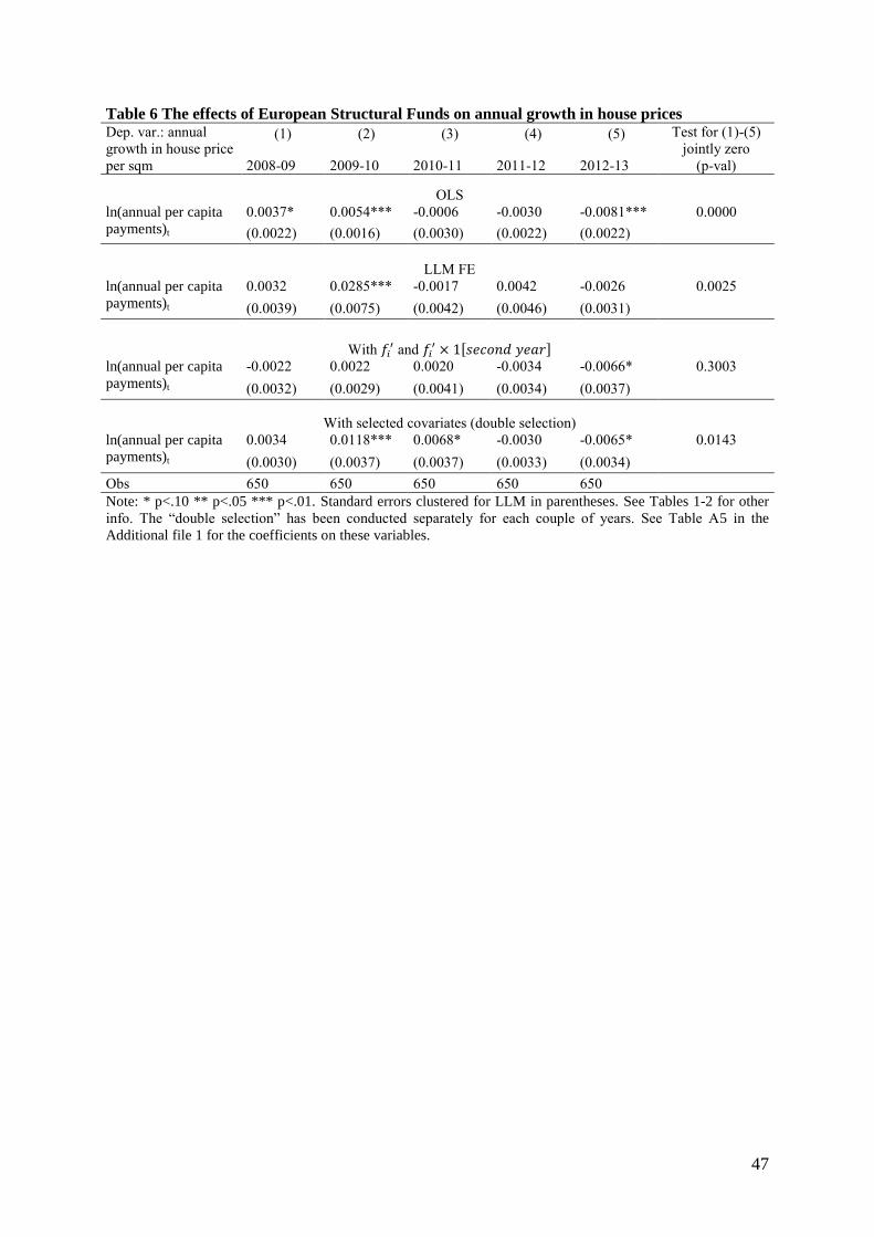
47

Table 6 The effects of European Structural Funds on annual growth in house prices Dep. var.: annual

growth in house price

per sqm

(1) (2) (3) (4) (5) Test for (1)-(5)

jointly zero

(p-val) 2008-09 2009-10 2010-11 2011-12 2012-13

OLS

ln(annual per capita

payments)t

0.0037* 0.0054*** -0.0006 -0.0030 -0.0081*** 0.0000

(0.0022) (0.0016) (0.0030) (0.0022) (0.0022)

LLM FE

ln(annual per capita

payments)t

0.0032 0.0285*** -0.0017 0.0042 -0.0026 0.0025

(0.0039) (0.0075) (0.0042) (0.0046) (0.0031)

With 𝑓𝑖′ and 𝑓𝑖

′ × 1[𝑠𝑒𝑐𝑜𝑛𝑑𝑦𝑒𝑎𝑟]

ln(annual per capita

payments)t

-0.0022 0.0022 0.0020 -0.0034 -0.0066* 0.3003

(0.0032) (0.0029) (0.0041) (0.0034) (0.0037)

With selected covariates (double selection)

ln(annual per capita

payments)t

0.0034 0.0118*** 0.0068* -0.0030 -0.0065* 0.0143

(0.0030) (0.0037) (0.0037) (0.0033) (0.0034)

Obs 650 650 650 650 650

Note: * p<.10 ** p<.05 *** p<.01. Standard errors clustered for LLM in parentheses. See Tables 1-2 for other

info. The “double selection” has been conducted separately for each couple of years. See Table A5 in the

Additional file 1 for the coefficients on these variables.

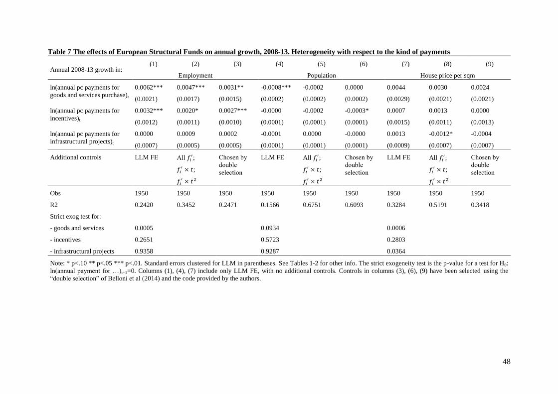
48

Table 7 The effects of European Structural Funds on annual growth, 2008-13. Heterogeneity with respect to the kind of payments

Annual 2008-13 growth in: (1) (2) (3) (4) (5) (6) (7) (8) (9)

Employment Population House price per sqm

ln(annual pc payments for

goods and services purchase)t

0.0062*** 0.0047*** 0.0031** -0.0008*** -0.0002 0.0000 0.0044 0.0030 0.0024

(0.0021) (0.0017) (0.0015) (0.0002) (0.0002) (0.0002) (0.0029) (0.0021) (0.0021)

ln(annual pc payments for

incentives)t

0.0032*** 0.0020* 0.0027*** -0.0000 -0.0002 -0.0003* 0.0007 0.0013 0.0000

(0.0012) (0.0011) (0.0010) (0.0001) (0.0001) (0.0001) (0.0015) (0.0011) (0.0013)

ln(annual pc payments for

infrastructural projects)t

0.0000 0.0009 0.0002 -0.0001 0.0000 -0.0000 0.0013 -0.0012* -0.0004

(0.0007) (0.0005) (0.0005) (0.0001) (0.0001) (0.0001) (0.0009) (0.0007) (0.0007)

Additional controls LLM FE All 𝑓𝑖′;

𝑓𝑖′ × 𝑡;

𝑓𝑖′ × 𝑡2

Chosen by

double

selection

LLM FE All 𝑓𝑖′;

𝑓𝑖′ × 𝑡;

𝑓𝑖′ × 𝑡2

Chosen by

double

selection

LLM FE All 𝑓𝑖′;

𝑓𝑖′ × 𝑡;

𝑓𝑖′ × 𝑡2

Chosen by

double

selection

Obs 1950 1950 1950 1950 1950 1950 1950 1950 1950

R2 0.2420 0.3452 0.2471 0.1566 0.6751 0.6093 0.3284 0.5191 0.3418

Strict exog test for:

- goods and services 0.0005 0.0934 0.0006

- incentives 0.2651 0.5723 0.2803

- infrastructural projects 0.9358 0.9287 0.0364

Note: * p<.10 ** p<.05 *** p<.01. Standard errors clustered for LLM in parentheses. See Tables 1-2 for other info. The strict exogeneity test is the p-value for a test for H0:

ln(annual payment for …)t+1=0. Columns (1), (4), (7) include only LLM FE, with no additional controls. Controls in columns (3), (6), (9) have been selected using the

“double selection” of Belloni et al (2014) and the code provided by the authors.

49

Table 8 The effects of European Structural Funds on annual growth, 2008-13. Heterogeneity with respect to slackness in the housing and labor

markets

Annual 2008-13 growth in: (1) (2) (3) (4) (5) (6) (7) (8) (9)

Employment Population House price per sqm

ln(annual pc payments)t 0.0027 -0.0008 0.0010 -0.0006*** -0.0001 -0.0005** 0.0064** 0.0021 0.0035

(0.0020) (0.0020) (0.0016) (0.0002) (0.0003) (0.0002) (0.0027) (0.0022) (0.0022)

ln(annual pc payments)t ×

housing slack indicator

0.0012 0.0032 0.0020 0.0005* 0.0004 0.0007** -0.0066* -0.0022 -0.0064*

(0.0025) (0.0022) (0.0021) (0.0003) (0.0004) (0.0003) (0.0036) (0.0031) (0.0034)

ln(annual pc payments)t ×

labor mkt slack indicator

-0.0011 0.0049* -0.0007 0.0002 -0.0002 0.0000 0.0100*** -0.0007 0.0076**

(0.0027) (0.0028) (0.0022) (0.0003) (0.0004) (0.0004) (0.0033) (0.0027) (0.0030)

housing slack indicator -0.0150 -0.0118 -0.0022 -0.0041** 0.0183 0.0381**

(0.0100) (0.0095) (0.0018) (0.0017) (0.0142) (0.0155)

labor mkt slack indicator -0.0214* 0.0057 0.0026 0.0006 0.0054 -0.0321**

(0.0126) (0.0099) (0.0020) (0.0018) (0.0129) (0.0142)

Additional controls LLM FE All 𝑓𝑖′;

𝑓𝑖′ × 𝑡;

𝑓𝑖′ × 𝑡2

Chosen by

double

selection

LLM FE All 𝑓𝑖′;

𝑓𝑖′ × 𝑡;

𝑓𝑖′ × 𝑡2

Chosen by

double

selection

LLM FE All 𝑓𝑖′;

𝑓𝑖′ × 𝑡;

𝑓𝑖′ × 𝑡2

Chosen by

double

selection

Obs 1950 1950 1950 1950 1950 1950 1950 1950 1950

R2 0.2352 0.3415 0.2366 0.1550 0.6771 0.5973 0.3368 0.5191 0.3167

Note: * p<.10 ** p<.05 *** p<.01. Standard errors clustered for LLM in parentheses. See Table 2 for other info. The housing slack indicator is a dummy for the lowest

quintile of housing prices across all LLMs in 2007. The labor market slack is a dummy for the lowest quintile of employment rate in 2007. Columns (1), (4), (7) include

only LLM FE, with no additional controls. To avoid introducing an additional source of variation, controls in columns (3), (6), (9) are the same selected for Table 2.

50

Table 9 The effects of the usage of European Structural Funds on average 2008-13 growth, controlling

for LLM time invariant characteristics

(1) (2) (3) (4) (5) (6)

Average 2008-2013 growth in:

Employment Population House price per sqm

Fraction of funds used in

2007-13 ([0-1] scale)

0.0004 -0.0051 -0.0005 -0.0015 -0.0299*** -0.0411***

(0.0057) (0.0060) (0.0017) (0.0016) (0.0114) (0.0107)

Controls selected by the double selection procedure:

ln(allocated per capita

funds)

-0.0156 -0.0030** 0.0023 0.0001 -0.0134 0.0000

(0.0126) (0.0012) (0.0037) (0.0004) (0.0293) (0.0024)

Fraction of surface

composed of

municipalities on the coast

-0.0017 0.0004 0.0017*** 0.0112**

(0.0022) (0.0007) (0.0005) (0.0048)

ln(house price per sqm)2005 0.0543*** 0.0052*** -0.0002 0.0123

(0.0183) (0.0017) (0.0054) (0.0309)

ln(employment)2006 0.1354 -0.0466 0.0005*** 1.6803***

(0.2105) (0.0552) (0.0002) (0.3537)

ln(house price per sqm)2006 0.0010 0.0015 -0.1567*** -0.0300***

(0.0160) (0.0051) (0.0333) (0.0036)

Empl rate2007 0.4741 -0.0038 0.1419 0.0032 1.5045 0.2700***

(0.9156) (0.0181) (0.2766) (0.0055) (2.2212) (0.0378)

ln(house price per sqm)2007 -0.0666** 0.0260*** 0.0007 0.0235

(0.0284) (0.0083) (0.0005) (0.0917)

population growth 2004-07 -0.3565 0.2178*** 0.0806 0.2144*** -0.3818

(1.3934) (0.0330) (0.4171) (0.0108) (3.0219)

Additional controls

All

remaining

vars in 𝑓𝑖′

No additional

controls

All

remaining

vars in 𝑓𝑖′

No additional

controls

All

remaining

vars in 𝑓𝑖′

No additional

controls

Obs 325 325 325 325 325 325

R2 0.5031 0.2695 0.8396 0.7778 0.4862 0.2429

Note: * p<.10 ** p<.05 *** p<.01. The unit of observation is the LLM over time. See Table 1 for data sources. The

regressions include a constant. Robust standard errors in parentheses. The average change over 2007-13 is calculated as

a geometric average. 𝑓𝑖′ is a vector of pre-determined covariates (see Table 2). Controls in columns (2), (4), (6) have

been selected using the “double selection” of Belloni et al (2014) and the code provided by the authors. Columns (1),

(3), (5) include all 𝑓𝑖′, but only coefficients on those that are also “double selected” are shown (a full regression table is

available from the authors).

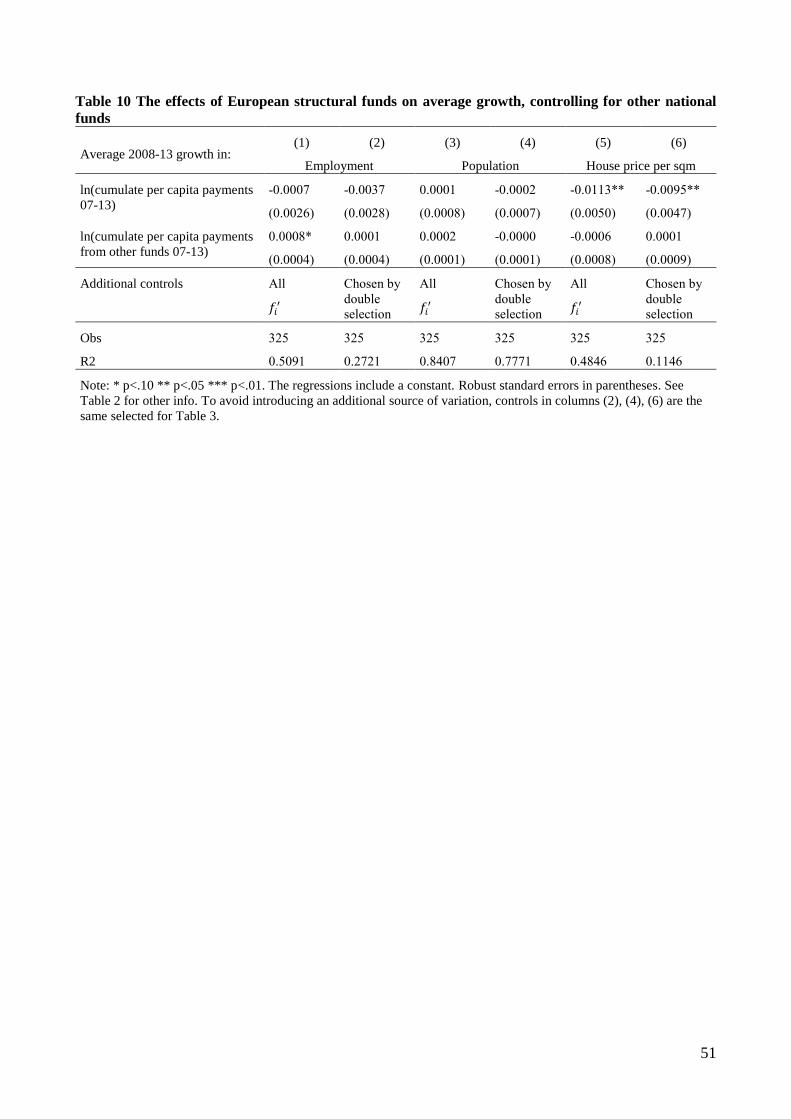
51

Table 10 The effects of European structural funds on average growth, controlling for other national

funds

Average 2008-13 growth in: (1) (2) (3) (4) (5) (6)

Employment Population House price per sqm

ln(cumulate per capita payments

07-13)

-0.0007 -0.0037 0.0001 -0.0002 -0.0113** -0.0095**

(0.0026) (0.0028) (0.0008) (0.0007) (0.0050) (0.0047)

ln(cumulate per capita payments

from other funds 07-13)

0.0008* 0.0001 0.0002 -0.0000 -0.0006 0.0001

(0.0004) (0.0004) (0.0001) (0.0001) (0.0008) (0.0009)

Additional controls All

𝑓𝑖′

Chosen by

double

selection

All

𝑓𝑖′

Chosen by

double

selection

All

𝑓𝑖′

Chosen by

double

selection

Obs 325 325 325 325 325 325

R2 0.5091 0.2721 0.8407 0.7771 0.4846 0.1146

Note: * p<.10 ** p<.05 *** p<.01. The regressions include a constant. Robust standard errors in parentheses. See

Table 2 for other info. To avoid introducing an additional source of variation, controls in columns (2), (4), (6) are the

same selected for Table 3.

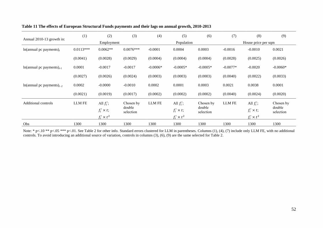
52

Table 11 The effects of European Structural Funds payments and their lags on annual growth, 2010-2013

Annual 2010-13 growth in: (1) (2) (3) (4) (5) (6) (7) (8) (9)

Employment Population House price per sqm

ln(annual pc payments)t 0.0113*** 0.0062** 0.0076*** -0.0001 0.0004 0.0003 -0.0016 -0.0010 0.0021

(0.0041) (0.0028) (0.0029) (0.0004) (0.0004) (0.0004) (0.0028) (0.0025) (0.0026)

ln(annual pc payments)t-1 0.0001 -0.0017 -0.0017 -0.0006* -0.0005* -0.0005* -0.0077* -0.0020 -0.0060*

(0.0027) (0.0026) (0.0024) (0.0003) (0.0003) (0.0003) (0.0040) (0.0022) (0.0033)

ln(annual pc payments)t -2 0.0002 -0.0000 -0.0010 0.0002 0.0001 0.0003 0.0021 0.0038 0.0001

(0.0021) (0.0019) (0.0017) (0.0002) (0.0002) (0.0002) (0.0040) (0.0024) (0.0020)

Additional controls LLM FE All 𝑓𝑖′;

𝑓𝑖′ × 𝑡;

𝑓𝑖′ × 𝑡2

Chosen by

double

selection

LLM FE All 𝑓𝑖′;

𝑓𝑖′ × 𝑡;

𝑓𝑖′ × 𝑡2

Chosen by

double

selection

LLM FE All 𝑓𝑖′;

𝑓𝑖′ × 𝑡;

𝑓𝑖′ × 𝑡2

Chosen by

double

selection

Obs 1300 1300 1300 1300 1300 1300 1300 1300 1300

Note: * p<.10 ** p<.05 *** p<.01. See Table 2 for other info. Standard errors clustered for LLM in parentheses. Columns (1), (4), (7) include only LLM FE, with no additional

controls. To avoid introducing an additional source of variation, controls in columns (3), (6), (9) are the same selected for Table 2.

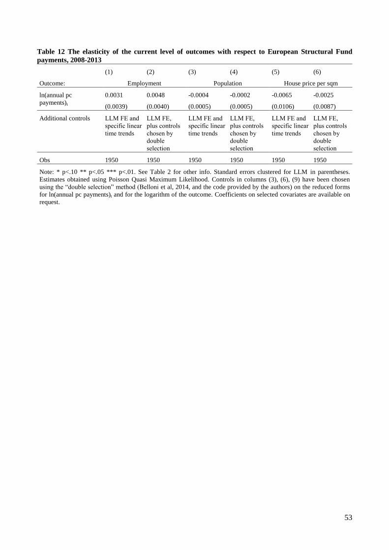
53

Table 12 The elasticity of the current level of outcomes with respect to European Structural Fund

payments, 2008-2013

(1) (2) (3) (4) (5) (6)

Outcome: Employment Population House price per sqm

ln(annual pc

payments)t

0.0031 0.0048 -0.0004 -0.0002 -0.0065 -0.0025

(0.0039) (0.0040) (0.0005) (0.0005) (0.0106) (0.0087)

Additional controls LLM FE and

specific linear

time trends

LLM FE,

plus controls

chosen by

double

selection

LLM FE and

specific linear

time trends

LLM FE,

plus controls

chosen by

double

selection

LLM FE and

specific linear

time trends

LLM FE,

plus controls

chosen by

double

selection

Obs 1950 1950 1950 1950 1950 1950

Note: * p<.10 ** p<.05 *** p<.01. See Table 2 for other info. Standard errors clustered for LLM in parentheses.

Estimates obtained using Poisson Quasi Maximum Likelihood. Controls in columns (3), (6), (9) have been chosen

using the “double selection” method (Belloni et al, 2014, and the code provided by the authors) on the reduced forms

for ln(annual pc payments)t and for the logarithm of the outcome. Coefficients on selected covariates are available on

request.

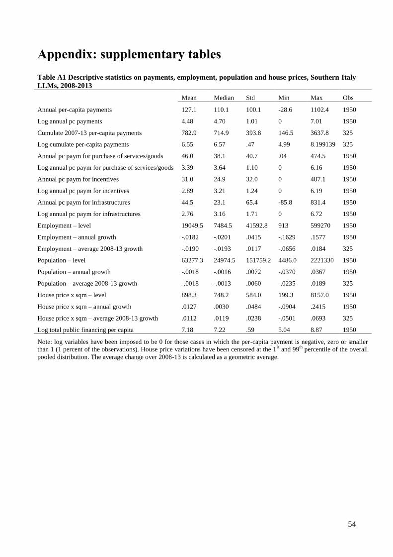
54

Appendix: supplementary tables

Table A1 Descriptive statistics on payments, employment, population and house prices, Southern Italy

LLMs, 2008-2013

Mean Median Std Min Max Obs

Annual per-capita payments 127.1 110.1 100.1 -28.6 1102.4 1950

Log annual pc payments 4.48 4.70 1.01 0 7.01 1950

Cumulate 2007-13 per-capita payments 782.9 714.9 393.8 146.5 3637.8 325

Log cumulate per-capita payments 6.55 6.57 .47 4.99 8.199139 325

Annual pc paym for purchase of services/goods 46.0 38.1 40.7 .04 474.5 1950

Log annual pc paym for purchase of services/goods 3.39 3.64 1.10 0 6.16 1950

Annual pc paym for incentives 31.0 24.9 32.0 0 487.1 1950

Log annual pc paym for incentives 2.89 3.21 1.24 0 6.19 1950

Annual pc paym for infrastructures 44.5 23.1 65.4 -85.8 831.4 1950

Log annual pc paym for infrastructures 2.76 3.16 1.71 0 6.72 1950

Employment – level 19049.5 7484.5 41592.8 913 599270 1950

Employment – annual growth -.0182 -.0201 .0415 -.1629 .1577 1950

Employment – average 2008-13 growth -.0190 -.0193 .0117 -.0656 .0184 325

Population – level 63277.3 24974.5 151759.2 4486.0 2221330 1950

Population – annual growth -.0018 -.0016 .0072 -.0370 .0367 1950

Population – average 2008-13 growth -.0018 -.0013 .0060 -.0235 .0189 325

House price x sqm – level 898.3 748.2 584.0 199.3 8157.0 1950

House price x sqm – annual growth .0127 .0030 .0484 -.0904 .2415 1950

House price x sqm – average 2008-13 growth .0112 .0119 .0238 -.0501 .0693 325

Log total public financing per capita 7.18 7.22 .59 5.04 8.87 1950

Note: log variables have been imposed to be 0 for those cases in which the per-capita payment is negative, zero or smaller

than 1 (1 percent of the observations). House price variations have been censored at the 1st and 99

th percentile of the overall

pooled distribution. The average change over 2008-13 is calculated as a geometric average.

55

Table A2 Descriptive statistics on other covariates (obs=325)

Mean Median Std Min Max

Surface (sqkm) 377.9 282.7 308.6 10.36 1686.0

Average altitude 389.4 370.3 241.0 5.2 1042.1

Fraction of surface in towns on the coast .2743 0 .3464 0 1

Frac of surface in towns in mountain area .6418 .8341 .3970 0 1

Residential units pc(2001) .5699 .5363 .1691 .3125 1.6477

Empty residential units pc (2001) .1985 .1594 .1573 .0216 1.2804

Population density 2007 193.3 91.5 347.1 12.0 3932.9

Unemployment rate 2004 .1361 .1312 .0390 .0552 .2771

Employment rate 2004 .3693 .3667 .0381 .2566 .4842

Activity rate 2004 .4269 .4224 .0331 .3297 .5393

Log population 2004 10.31 10.13 1.07 8.55 14.62

Log employment 2004 9.14 8.93 1.08 7.30 13.40

Log house price x sqm 2004 6.41 6.36 .38 5.61 8.85

Unemployment rate 2005 .1323 .1285 .0323 .0503 .2514

Employment rate 2005 .3653 .3615 .0375 .2627 .4889

Activity rate 2005 .4204 .4163 .0339 .3263 .5508

Log population 2005 10.31 10.13 1.07 8.54 14.62

Log employment 2005 9.14 8.93 1.08 7.23 13.37

Log house price x sqm 2005 6.50 6.43 .40 5.70 8.89

Unemployment rate 2006 .1125 .1104 .0277 .0509 .2168

Employment rate 2006 .3718 .3684 .0377 .2766 .4993

Activity rate 2006 .4185 .4171 .0355 .3248 .5412

Log population 2006 10.30 10.13 1.07 8.53 14.62

Log employment 2006 9.15 8.96 1.08 7.25 13.36

Log house price x sqm 2006 6.55 6.49 .40 5.71 8.95

Unemployment rate 2007 .1062 .1021 .0269 .0511 .2053

Employment rate 2007 .3683 .3641 .0387 .2581 .5075

Activity rate 2007 .4116 .4057 .0364 .3049 .5537

Log population 2007 10.30 10.13 1.08 8.52 14.61

Log employment 2007 9.15 8.98 1.09 7.22 13.33

Log house price x sqm 2007 6.62 6.56 .42 5.74 8.99

Employment: 2004-07 growth .0051 .0021 .0535 -.2445 .1764

Population: 2004-07 growth -.0089 -.0082 .0212 -.0781 .0897

House price x sqm: 2004-07 growth .2470 .1990 .1959 -.0802 1.298

Share construction in private empl 2007 .1747 .1671 .0494 .0851 .4062

Share trade and restaurants 2007 .3516 .3481 .0771 .1613 .6559

Share services 2007 .2711 .2641 .0580 .1333 .4769

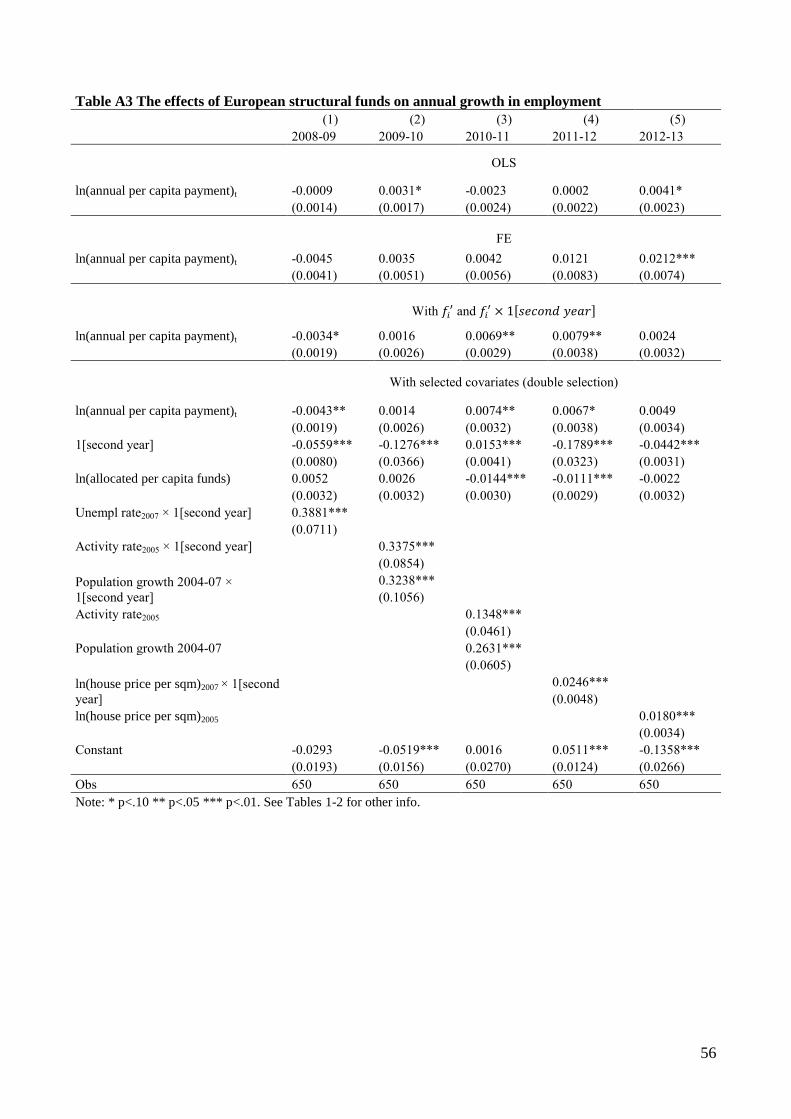
56

Table A3 The effects of European structural funds on annual growth in employment

(1) (2) (3) (4) (5)

2008-09 2009-10 2010-11 2011-12 2012-13

OLS

ln(annual per capita payment)t -0.0009 0.0031* -0.0023 0.0002 0.0041*

(0.0014) (0.0017) (0.0024) (0.0022) (0.0023)

FE

ln(annual per capita payment)t -0.0045 0.0035 0.0042 0.0121 0.0212***

(0.0041) (0.0051) (0.0056) (0.0083) (0.0074)

With 𝑓𝑖′ and 𝑓𝑖

′ × 1[𝑠𝑒𝑐𝑜𝑛𝑑𝑦𝑒𝑎𝑟]

ln(annual per capita payment)t -0.0034* 0.0016 0.0069** 0.0079** 0.0024

(0.0019) (0.0026) (0.0029) (0.0038) (0.0032)

With selected covariates (double selection)

ln(annual per capita payment)t -0.0043** 0.0014 0.0074** 0.0067* 0.0049

(0.0019) (0.0026) (0.0032) (0.0038) (0.0034)

1[second year] -0.0559*** -0.1276*** 0.0153*** -0.1789*** -0.0442***

(0.0080) (0.0366) (0.0041) (0.0323) (0.0031)

ln(allocated per capita funds) 0.0052 0.0026 -0.0144*** -0.0111*** -0.0022

(0.0032) (0.0032) (0.0030) (0.0029) (0.0032)

Unempl rate2007 × 1[second year] 0.3881***

(0.0711)

Activity rate2005 × 1[second year]

0.3375***

(0.0854)

Population growth 2004-07 ×

1[second year]

0.3238***

(0.1056)

Activity rate2005

0.1348***

(0.0461)

Population growth 2004-07

0.2631***

(0.0605)

ln(house price per sqm)2007 × 1[second

year]

0.0246***

(0.0048)

ln(house price per sqm)2005

0.0180***

(0.0034)

Constant -0.0293 -0.0519*** 0.0016 0.0511*** -0.1358***

(0.0193) (0.0156) (0.0270) (0.0124) (0.0266)

Obs 650 650 650 650 650

Note: * p<.10 ** p<.05 *** p<.01. See Tables 1-2 for other info.

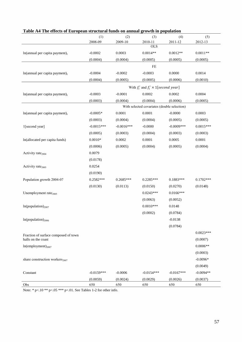
57

Table A4 The effects of European structural funds on annual growth in population

(1) (2) (3) (4) (5)

2008-09 2009-10 2010-11 2011-12 2012-13

OLS

ln(annual per capita payment)t -0.0002 0.0003 0.0014** 0.0012** 0.0011**

(0.0004) (0.0004) (0.0005) (0.0005) (0.0005)

FE

ln(annual per capita payment)t -0.0004 -0.0002 -0.0003 0.0000 0.0014

(0.0004) (0.0005) (0.0005) (0.0006) (0.0010)

With 𝑓𝑖′ and 𝑓𝑖

′ × 1[𝑠𝑒𝑐𝑜𝑛𝑑𝑦𝑒𝑎𝑟]

ln(annual per capita payment)t -0.0003 -0.0001 0.0002 0.0002 0.0004

(0.0003) (0.0004) (0.0004) (0.0006) (0.0005)

With selected covariates (double selection)

ln(annual per capita payment)t -0.0005* 0.0001 0.0001 -0.0000 0.0003

(0.0003) (0.0004) (0.0004) (0.0005) (0.0005)

1[second year] -0.0015*** -0.0016*** -0.0000 -0.0009*** 0.0015***

(0.0005) (0.0003) (0.0004) (0.0003) (0.0003)

ln(allocated per capita funds) 0.0010* 0.0002 0.0001 0.0005 0.0001

(0.0006) (0.0005) (0.0004) (0.0005) (0.0004)

Activity rate2004 0.0079

(0.0178)

Activity rate2005 0.0254

(0.0190)

Population growth 2004-07 0.2582*** 0.2685*** 0.2285*** 0.1883*** 0.1702***

(0.0130) (0.0113) (0.0150) (0.0270) (0.0148)

Unemployment rate2005

0.0243*** 0.0166***

(0.0063) (0.0052)

ln(population)2007

0.0010*** 0.0148

(0.0002) (0.0784)

ln(population)2006

-0.0138

(0.0784)

Fraction of surface composed of town

halls on the coast

0.0023***

(0.0007)

ln(employment)2007 0.0006**

(0.0003)

share construction workers2007 -0.0096*

(0.0049)

Constant -0.0159*** -0.0006 -0.0154*** -0.0167*** -0.0094**

(0.0059) (0.0024) (0.0029) (0.0026) (0.0037)

Obs 650 650 650 650 650

Note: * p<.10 ** p<.05 *** p<.01. See Tables 1-2 for other info.

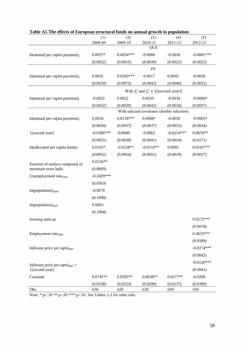
58

Table A5 The effects of European structural funds on annual growth in population

(1) (2) (3) (4) (5)

2008-09 2009-10 2010-11 2011-12 2012-13

OLS

ln(annual per capita payment)t 0.0037* 0.0054*** -0.0006 -0.0030 -0.0081***

(0.0022) (0.0016) (0.0030) (0.0022) (0.0022)

FE

ln(annual per capita payment)t 0.0032 0.0285*** -0.0017 0.0042 -0.0026

(0.0039) (0.0075) (0.0042) (0.0046) (0.0031)

With 𝑓𝑖′ and 𝑓𝑖

′ × 1[𝑠𝑒𝑐𝑜𝑛𝑑𝑦𝑒𝑎𝑟]

ln(annual per capita payment)t -0.0022 0.0022 0.0020 -0.0034 -0.0066*

(0.0032) (0.0029) (0.0041) (0.0034) (0.0037)

With selected covariates (double selection)

ln(annual per capita payment)t 0.0034 0.0118*** 0.0068* -0.0030 -0.0065*

(0.0030) (0.0037) (0.0037) (0.0033) (0.0034)

1[second year] -0.0386*** -0.0049 -0.0062 -0.0214*** 0.0676**

(0.0055) (0.0038) (0.0041) (0.0024) (0.0271)

ln(allocated per capita funds) 0.0102* -0.0128** -0.0110** 0.0001 0.0105***

(0.0052) (0.0056) (0.0051) (0.0029) (0.0027)

Fraction of surface composed of

mountain town halls

0.0156**

(0.0069)

Unemployment rate2004 -0.2429***

(0.0563)

ln(population)2004 -0.0679

(0.1099)

ln(population)2007 0.0603

(0.1094)

housing units pc 0.0272***

(0.0074)

Employment rate2006 0.3633***

(0.0589)

ln(house price per sqm)2007 -0.0274***

(0.0042)

ln(house price per sqm)2007 ×

1[second year]

-0.0120***

(0.0041)

Constant 0.0745** 0.0595** 0.0638** 0.0277** -0.0208

(0.0338) (0.0253) (0.0299) (0.0137) (0.0390)

Obs 650 650 650 650 650

Note: * p<.10 ** p<.05 *** p<.01. See Tables 1-2 for other info.

(*) Requests for copies should be sent to: Banca d’Italia – Servizio Struttura economica e finanziaria – Divisione Biblioteca e Archivio storico – Via Nazionale, 91 – 00184 Rome – (fax 0039 06 47922059). They are available on the Internet www.bancaditalia.it.

RECENTLY PUBLISHED “TEMI” (*)

N. 1005 – Strategy and tactics in public debt manamgement, by Davide Dottori and Michele Manna (March 2015).

N. 1006 – Inward foreign direct investment and innovation: evidence from Italian provinces, by Roberto Antonietti, Raffaello Bronzini and Giulio Cainelli (March 2015).

N. 1007 – The macroeconomic effects of the sovereign debt crisis in the euro area, by Stefano Neri and Tiziano Ropele (March 2015).

N. 1008 – Rethinking the crime reducing effect of education? Mechanisms and evidence from regional divides, by Ylenia Brilli and Marco Tonello (April 2015).

N. 1009 – Social capital and the cost of credit: evidence from a crisis, by Paolo Emilio Mistrulli and Valerio Vacca (April 2015).

N. 1010 – Every cloud has a silver lining. The sovereign crisis and Italian potential output, by Andrea Gerali, Alberto Locarno, Alessandro Notarpietro and Massimiliano Pisani (June 2015).

N. 1011 – Foreign direct investment and firm performance: an empirical analysis of Italian firms, by Alessandro Borin and Michele Mancini (June 2015).

N. 1012 – Sovereign debt and reserves with liquidity and productivity crises, by Flavia Corneli and Emanuele Tarantino (June 2015).

N. 1013 – Bankruptcy law and bank financing, by Giacomo Rodano, Nicolas Serrano-Velarde and Emanuele Tarantino (June 2015).

N. 1014 – Women as ‘gold dust’: gender diversity in top boards and the performance of Italian banks, by Silvia Del Prete and Maria Lucia Stefani (June 2015).

N. 1015 – Inflation, financial conditions and non-standard monetary policy in a monetary union. A model-based evaluation, by Lorenzo Burlon, Andrea Gerali, Alessandro Notarpietro and Massimiliano Pisani (June 2015).

N. 1016 – Short term inflation forecasting: the M.E.T.A. approach, by Giacomo Sbrana, Andrea Silvestrini and Fabrizio Venditti (June 2015).

N. 1017 – A note on social capital, space and growth in Europe, by Luciano Lavecchia (July 2015).

N. 1018 – Statistical matching and uncertainty analysis in combining household income and expenditure data, by Pier Luigi Conti, Daniela Marella and Andrea Neri (July 2015).

N. 1019 – Why is inflation so low in the euro area?, by Antonio M. Conti, Stefano Neri and Andrea Nobili (July 2015).

N. 1020 – Forecaster heterogeneity, surprises and financial markets, by Marcello Pericoli and Giovanni Veronese (July 2015).

N. 1021 – Decomposing euro area sovereign spreads: credit,liquidity and convenience, by Marcello Pericoli and Marco Taboga (July 2015).

N. 1022 – Testing information diffusion in the decentralized unsecured market for euro funds, by Edoardo Rainone (July 2015).

N. 1023 – Understanding policy rates at the zero lower bound: insights from a Bayesian shadow rate model, by Marcello Pericoli and Marco Taboga (July 2015).

N. 1024 – Accessorizing. The effect of union contract renewals on consumption, by Effrosyni Adamopoulou and Roberta Zizza (July 2015).

N. 1025 – Tail comovement in option-implied inflation expectations as an indicator of anchoring, by Sara Cecchetti, Filippo Natoli and Laura Sigalotti (July 2015).

N. 1026 – Follow the value added: bilateral gross export accounting, by Alessandro Borin and Michele Mancini (July 2015).

N. 1027 – On the conditional distribution of euro area inflation forecast, by Fabio Busetti, Michele Caivano and Lisa Rodano (July 2015).

"TEMI" LATER PUBLISHED ELSEWHERE

2013

A. MERCATANTI, A likelihood-based analysis for relaxing the exclusion restriction in randomized

experiments with imperfect compliance, Australian and New Zealand Journal of Statistics, v. 55, 2, pp. 129-153, TD No. 683 (August 2008).

F. CINGANO and P. PINOTTI, Politicians at work. The private returns and social costs of political connections, Journal of the European Economic Association, v. 11, 2, pp. 433-465, TD No. 709 (May 2009).

F. BUSETTI and J. MARCUCCI, Comparing forecast accuracy: a Monte Carlo investigation, International Journal of Forecasting, v. 29, 1, pp. 13-27, TD No. 723 (September 2009).

D. DOTTORI, S. I-LING and F. ESTEVAN, Reshaping the schooling system: The role of immigration, Journal of Economic Theory, v. 148, 5, pp. 2124-2149, TD No. 726 (October 2009).

A. FINICELLI, P. PAGANO and M. SBRACIA, Ricardian Selection, Journal of International Economics, v. 89, 1, pp. 96-109, TD No. 728 (October 2009).

L. MONTEFORTE and G. MORETTI, Real-time forecasts of inflation: the role of financial variables, Journal of Forecasting, v. 32, 1, pp. 51-61, TD No. 767 (July 2010).

R. GIORDANO and P. TOMMASINO, Public-sector efficiency and political culture, FinanzArchiv, v. 69, 3, pp. 289-316, TD No. 786 (January 2011).

E. GAIOTTI, Credit availablility and investment: lessons from the "Great Recession", European Economic Review, v. 59, pp. 212-227, TD No. 793 (February 2011).

F. NUCCI and M. RIGGI, Performance pay and changes in U.S. labor market dynamics, Journal of Economic Dynamics and Control, v. 37, 12, pp. 2796-2813, TD No. 800 (March 2011).

G. CAPPELLETTI, G. GUAZZAROTTI and P. TOMMASINO, What determines annuity demand at retirement?, The Geneva Papers on Risk and Insurance – Issues and Practice, pp. 1-26, TD No. 805 (April 2011).

A. ACCETTURO e L. INFANTE, Skills or Culture? An analysis of the decision to work by immigrant women in Italy, IZA Journal of Migration, v. 2, 2, pp. 1-21, TD No. 815 (July 2011).

A. DE SOCIO, Squeezing liquidity in a “lemons market” or asking liquidity “on tap”, Journal of Banking and Finance, v. 27, 5, pp. 1340-1358, TD No. 819 (September 2011).

S. GOMES, P. JACQUINOT, M. MOHR and M. PISANI, Structural reforms and macroeconomic performance in the euro area countries: a model-based assessment, International Finance, v. 16, 1, pp. 23-44, TD No. 830 (October 2011).

G. BARONE and G. DE BLASIO, Electoral rules and voter turnout, International Review of Law and Economics, v. 36, 1, pp. 25-35, TD No. 833 (November 2011).

O. BLANCHARD and M. RIGGI, Why are the 2000s so different from the 1970s? A structural interpretation of changes in the macroeconomic effects of oil prices, Journal of the European Economic Association, v. 11, 5, pp. 1032-1052, TD No. 835 (November 2011).

R. CRISTADORO and D. MARCONI, Household savings in China, in G. Gomel, D. Marconi, I. Musu, B. Quintieri (eds), The Chinese Economy: Recent Trends and Policy Issues, Springer-Verlag, Berlin, TD No. 838 (November 2011).

A. ANZUINI, M. J. LOMBARDI and P. PAGANO, The impact of monetary policy shocks on commodity prices, International Journal of Central Banking, v. 9, 3, pp. 119-144, TD No. 851 (February 2012).

R. GAMBACORTA and M. IANNARIO, Measuring job satisfaction with CUB models, Labour, v. 27, 2, pp. 198-224, TD No. 852 (February 2012).

G. ASCARI and T. ROPELE, Disinflation effects in a medium-scale new keynesian model: money supply rule versus interest rate rule, European Economic Review, v. 61, pp. 77-100, TD No. 867 (April 2012).

E. BERETTA and S. DEL PRETE, Banking consolidation and bank-firm credit relationships: the role of geographical features and relationship characteristics, Review of Economics and Institutions, v. 4, 3, pp. 1-46, TD No. 901 (February 2013).

M. ANDINI, G. DE BLASIO, G. DURANTON and W. STRANGE, Marshallian labor market pooling: evidence from Italy, Regional Science and Urban Economics, v. 43, 6, pp.1008-1022, TD No. 922 (July 2013).

G. SBRANA and A. SILVESTRINI, Forecasting aggregate demand: analytical comparison of top-down and bottom-up approaches in a multivariate exponential smoothing framework, International Journal of Production Economics, v. 146, 1, pp. 185-98, TD No. 929 (September 2013).

A. FILIPPIN, C. V, FIORIO and E. VIVIANO, The effect of tax enforcement on tax morale, European Journal of Political Economy, v. 32, pp. 320-331, TD No. 937 (October 2013).

2014

G. M. TOMAT, Revisiting poverty and welfare dominance, Economia pubblica, v. 44, 2, 125-149, TD No. 651

(December 2007).

M. TABOGA, The riskiness of corporate bonds, Journal of Money, Credit and Banking, v.46, 4, pp. 693-713, TD No. 730 (October 2009).

G. MICUCCI and P. ROSSI, Il ruolo delle tecnologie di prestito nella ristrutturazione dei debiti delle imprese in crisi, in A. Zazzaro (a cura di), Le banche e il credito alle imprese durante la crisi, Bologna, Il Mulino, TD No. 763 (June 2010).

F. D’AMURI, Gli effetti della legge 133/2008 sulle assenze per malattia nel settore pubblico, Rivista di politica economica, v. 105, 1, pp. 301-321, TD No. 787 (January 2011).

R. BRONZINI and E. IACHINI, Are incentives for R&D effective? Evidence from a regression discontinuity approach, American Economic Journal : Economic Policy, v. 6, 4, pp. 100-134, TD No. 791 (February 2011).

P. ANGELINI, S. NERI and F. PANETTA, The interaction between capital requirements and monetary policy, Journal of Money, Credit and Banking, v. 46, 6, pp. 1073-1112, TD No. 801 (March 2011).

M. BRAGA, M. PACCAGNELLA and M. PELLIZZARI, Evaluating students’ evaluations of professors, Economics of Education Review, v. 41, pp. 71-88, TD No. 825 (October 2011).

M. FRANCESE and R. MARZIA, Is there Room for containing healthcare costs? An analysis of regional spending differentials in Italy, The European Journal of Health Economics, v. 15, 2, pp. 117-132, TD No. 828 (October 2011).

L. GAMBACORTA and P. E. MISTRULLI, Bank heterogeneity and interest rate setting: what lessons have we learned since Lehman Brothers?, Journal of Money, Credit and Banking, v. 46, 4, pp. 753-778, TD No. 829 (October 2011).

M. PERICOLI, Real term structure and inflation compensation in the euro area, International Journal of Central Banking, v. 10, 1, pp. 1-42, TD No. 841 (January 2012).

E. GENNARI and G. MESSINA, How sticky are local expenditures in Italy? Assessing the relevance of the flypaper effect through municipal data, International Tax and Public Finance, v. 21, 2, pp. 324-344, TD No. 844 (January 2012).

V. DI GACINTO, M. GOMELLINI, G. MICUCCI and M. PAGNINI, Mapping local productivity advantages in Italy: industrial districts, cities or both?, Journal of Economic Geography, v. 14, pp. 365–394, TD No. 850 (January 2012).

A. ACCETTURO, F. MANARESI, S. MOCETTI and E. OLIVIERI, Don't Stand so close to me: the urban impact of immigration, Regional Science and Urban Economics, v. 45, pp. 45-56, TD No. 866 (April 2012).

M. PORQUEDDU and F. VENDITTI, Do food commodity prices have asymmetric effects on euro area inflation, Studies in Nonlinear Dynamics and Econometrics, v. 18, 4, pp. 419-443, TD No. 878 (September 2012).

S. FEDERICO, Industry dynamics and competition from low-wage countries: evidence on Italy, Oxford Bulletin of Economics and Statistics, v. 76, 3, pp. 389-410, TD No. 879 (September 2012).

F. D’AMURI and G. PERI, Immigration, jobs and employment protection: evidence from Europe before and during the Great Recession, Journal of the European Economic Association, v. 12, 2, pp. 432-464, TD No. 886 (October 2012).

M. TABOGA, What is a prime bank? A euribor-OIS spread perspective, International Finance, v. 17, 1, pp. 51-75, TD No. 895 (January 2013).

G. CANNONE and D. FANTINO, Evaluating the efficacy of european regional funds for R&D, Rassegna italiana di valutazione, v. 58, pp. 165-196, TD No. 902 (February 2013).

L. GAMBACORTA and F. M. SIGNORETTI, Should monetary policy lean against the wind? An analysis based on a DSGE model with banking, Journal of Economic Dynamics and Control, v. 43, pp. 146-74, TD No. 921 (July 2013).

M. BARIGOZZI, CONTI A.M. and M. LUCIANI, Do euro area countries respond asymmetrically to the common monetary policy?, Oxford Bulletin of Economics and Statistics, v. 76, 5, pp. 693-714, TD No. 923 (July 2013).

U. ALBERTAZZI and M. BOTTERO, Foreign bank lending: evidence from the global financial crisis, Journal of International Economics, v. 92, 1, pp. 22-35, TD No. 926 (July 2013).

R. DE BONIS and A. SILVESTRINI, The Italian financial cycle: 1861-2011, Cliometrica, v.8, 3, pp. 301-334, TD No. 936 (October 2013).

G. BARONE and S. MOCETTI, Natural disasters, growth and institutions: a tale of two earthquakes, Journal of Urban Economics, v. 84, pp. 52-66, TD No. 949 (January 2014).

D. PIANESELLI and A. ZAGHINI, The cost of firms’ debt financing and the global financial crisis, Finance Research Letters, v. 11, 2, pp. 74-83, TD No. 950 (February 2014).

A. ZAGHINI, Bank bonds: size, systemic relevance and the sovereign, International Finance, v. 17, 2, pp. 161-183, TD No. 966 (July 2014).

G. SBRANA and A. SILVESTRINI, Random switching exponential smoothing and inventory forecasting, International Journal of Production Economics, v. 156, 1, pp. 283-294, TD No. 971 (October 2014).

M. SILVIA, Does issuing equity help R&D activity? Evidence from unlisted Italian high-tech manufacturing firms, Economics of Innovation and New Technology, v. 23, 8, pp. 825-854, TD No. 978 (October 2014).

2015

M. BUGAMELLI, S. FABIANI and E. SETTE, The age of the dragon: the effect of imports from China on firm-

level prices, Journal of Money, Credit and Banking, v. 47, 6, pp. 1091-1118, TD No. 737 (January 2010).

G. BULLIGAN, M. MARCELLINO and F. VENDITTI, Forecasting economic activity with targeted predictors, International Journal of Forecasting, v. 31, 1, pp. 188-206, TD No. 847 (February 2012).

A. CIARLONE, House price cycles in emerging economies, Studies in Economics and Finance, v. 32, 1, TD No. 863 (May 2012).

D. FANTINO, A. MORI and D. SCALISE, Collaboration between firms and universities in Italy: the role of a firm's proximity to top-rated departments, Rivista Italiana degli economisti, v. 1, 2, pp. 219-251, TD No. 884 (October 2012).

G. BARONE and G. NARCISO, Organized crime and business subsidies: Where does the money go?, Journal of Urban Economics, v. 86, pp. 98-110, TD No. 916 (June 2013).

P. ALESSANDRI and B. NELSON, Simple banking: profitability and the yield curve, Journal of Money, Credit and Banking, v. 47, 1, pp. 143-175, TD No. 945 (January 2014).

R. AABERGE and A. BRANDOLINI, Multidimensional poverty and inequality, in A. B. Atkinson and F. Bourguignon (eds.), Handbook of Income Distribution, Volume 2A, Amsterdam, Elsevier, TD No. 976 (October 2014).

V. CUCINIELLO and F. M. SIGNORETTI, Large banks,loan rate markup and monetary policy, International Journal of Central Banking, v. 11, 3, pp. 141-177, TD No. 987 (November 2014).

M. FRATZSCHER, D. RIMEC, L. SARNOB and G. ZINNA, The scapegoat theory of exchange rates: the first tests, Journal of Monetary Economics, v. 70, 1, pp. 1-21, TD No. 991 (November 2014).

A. NOTARPIETRO and S. SIVIERO, Optimal monetary policy rules and house prices: the role of financial frictions, Journal of Money, Credit and Banking, v. 47, S1, pp. 383-410, TD No. 993 (November 2014).

R. ANTONIETTI, R. BRONZINI and G. CAINELLI, Inward greenfield FDI and innovation, Economia e Politica Industriale, v. 42, 1, pp. 93-116, TD No. 1006 (March 2015).

FORTHCOMING

G. DE BLASIO, D. FANTINO and G. PELLEGRINI, Evaluating the impact of innovation incentives: evidence from an unexpected shortage of funds, Industrial and Corporate Change, TD No. 792 (February 2011).

A. DI CESARE, A. P. STORK and C. DE VRIES, Risk measures for autocorrelated hedge fund returns, Journal of Financial Econometrics, TD No. 831 (October 2011).

E. BONACCORSI DI PATTI and E. SETTE, Did the securitization market freeze affect bank lending during the financial crisis? Evidence from a credit register, Journal of Financial Intermediation, TD No. 848 (February 2012).

M. MARCELLINO, M. PORQUEDDU and F. VENDITTI, Short-Term GDP Forecasting with a mixed frequency dynamic factor model with stochastic volatility, Journal of Business & Economic Statistics, TD No. 896 (January 2013).

M. ANDINI and G. DE BLASIO, Local development that money cannot buy: Italy’s Contratti di Programma, Journal of Economic Geography, TD No. 915 (June 2013).

J. LI and G. ZINNA, On bank credit risk: sytemic or bank-specific? Evidence from the US and UK, Journal of Financial and Quantitative Analysis, TD No. 951 (February 2015).

A. L. MANCINI, C. MONFARDINI and S. PASQUA, Is a good example the best sermon? Children’s imitation of parental reading, Review of Economics of the Household, TD No. 958 (April 2014).

L. BURLON, Public expenditure distribution, voting, and growth, Journal of Public Economic Theory, TD No. 961 (April 2014).

A. BRANDOLINI and E. VIVIANO, Behind and beyond the (headcount) employment rate, Journal of the Royal Statistical Society: Series A, TD No. 965 (July 2015).