technology portfolio analysis for residential … portfolio analysis for residential lighting ......

WP-2007-007

Technology portfolio analysis for residential lighting

P. Balachandra and B. Sudhakara Reddy

Indira Gandhi Institute of Development Research, Mumbai May 2007


P. Balachandra Department of Management Studies

Indian Institute of Science, Bangalore-560012, INDIA

B. Sudhakara Reddy

Indira Gandhi Institute of Development Research (IGIDR) General Arun Kumar Vaidya Marg

Goregaon (E), Mumbai- 400065, INDIA Email (corresponding author): [email protected]

Abstract Electricity consumption in India is increasing rapidly over the years. The increased demand for electricity forces the electricity utilities to increase their generating capacity. The huge investments on generation, transmission and distribution (at the cost of alternative development projects) adversely affect India's scarce capital resources. Also, internal energy resources like coal are utilised with a great risk to the environment. This paper attempts to show analytically the benefits of shift in the focus from supply augmentation to demand management through a case study of replacement of inefficient devices with efficient ones for residential lighting. This is being done by analyzing the economics of various alternatives and developing an optimal portfolio for meeting the lighting requirement of a typical household in Maharashtra State in India. A mixed integer-programming model has been used for developing the optimal portfolio and a comparison of annual returns is made. Finally, the results for the typical household have been extended to the state of Maharashtra and the cost and benefits are estimated. The results show that the optimal lighting portfolio provides a far higher return at a lower risk compared to other investment alternatives like the stock market while providing substantial savings both in terms of energy and peak demand. Key words: Demand management, electricity consumption, energy resources, mixed integer-programming model, rate of return JEL Code: Q4

2


P. Balachandra and B. Sudhakara Reddy

1. Introduction

India's demand for electricity has been increasing over the years. The electricity

consumption in 1979-80 was 78,123 GWh and increased to 339,598 GWh during 2002-2003,

an increase of about 6.6% per annum. The share of Maharashtra, a state in Western India, in

the total electricity consumption is the highest in India (17%). As development continues, the

future demand and the real cost of producing a kilowatt of electricity will increase

significantly. As a result, enormous amounts of scarce capital should be invested on

generation, transmission and distribution. Also, financial, environmental and energy resource

constraints limit the expansion of the supply capacity resulting in severe shortages. With

increasing demands and rising costs of generation, the question is how to reduce demand

without compromising on services. Energy efficiency may partly fill this gap. The supply

expansion can be deferred, at least partly, if the existing inefficient devices/appliances are

replaced with efficient ones. From an individual's point of view, energy efficiency can be

viewed as an investment opportunity in which the initial cost is weighed against future

returns in the form of subsequent reductions in expected energy costs.

In the residential sector, lighting is one of the most important uses of electrical energy.

It represents 10 to 20% of electricity use in most countries and sometimes more in developing

countries (Dutt, 1994). The technological advances in lighting technologies have resulted in

improvement of lighting energy efficiency by a factor of five without any alteration in light

levels. Though the potentials in terms of energy savings and economic returns of these efficient

lighting technologies have been recognised, penetration rates into the market are very low

3

(Gadgil and Jannuzzi, 1994). One of the main reasons for this is the high initial capital costs.

For example, in India, the purchase cost of compact fluorescent lamps is almost 15 to 20 times

that of incandescent bulbs, and thrice that of fluorescent tubes. Also, the individual adopters

tend to use very high discount rates to evaluate energy-efficient technologies (Metcaff, 1994).

In India typical middle-income investors use a discount rate as high as 40% to evaluate energy

efficient devices (Reddy, 1996).

One possible way of improving the market penetration rates of efficient technologies

could be to sell them as “lighting packages” consisting of a “portfolio” of both inefficient and

efficient lighting, which may help in diversifying the risk associated with investments in

efficient devices. In addition, this can facilitate an effective match between lighting technology

and lighting levels required. The concept of portfolio theory deals with the efficient

combination of risk assets into a single portfolio in which each asset is characterised by its

expected rate of return, its risk, and the risk relative to that of other assets in the portfolio (Levy

and Sarnat, 1994). A majority of the work related to the choice of energy efficient technologies

(based on their economic performances) is done on the basis of these security analyses wherein

only the costs and returns of these technologies are estimated without giving any attention to

the risk associated with them (Sutherland, 1986 and Sutherland, 1991). That is, the choice of a

technology was entirely based either on least cost or on maximum returns. However, recent

literature identifies the need for the inclusion of the risk in the investment analysis of modeling

energy technology choices (Sutherland, 1991 and Johnson, 1994). It may be a rational

proposition to have a portfolio of existing inefficient and efficient technologies rather than

having complete replacement of inefficient technologies with efficient ones. A similar approach

was attempted by Sutherland (1986) to compare investments in nuclear and coal-based power

plants.

4

The present paper deals with energy efficiency by looking at the individual as well as

societal perspectives. This will be done by attempting to answer the following questions, viz.,

(i) is it possible to view energy efficient technology as an attractive investment alternative

comparable to the common stock option? (ii) Considering the high investment required for the

efficient alternatives and the risks involved, is there an optimal mix of energy technologies,

which is reasonably efficient and provides high returns at low risks? (iii) If an optimal portfolio

can be developed, then what are the benefits that could accrue to the residential sector and the

state as whole? Thus, the main objective of this study is to answer these questions by analysing

the feasible energy efficient lighting technologies and developing an optimal portfolio of them

to meet the lighting requirements of residential consumer. This optimal portfolio is expected to

have such alternatives of lighting technologies, which provide maximum returns to the

individual consumers under given constraints. Lighting for a typical household in Maharashtra

State is considered as an example for this exercise. Finally, the results are extended to the

residential sector of the state.

The present study analyses the economic and technical feasibility of all the available

lighting alternatives and then attempts to construct an optimal portfolio of these alternatives

for meeting the lighting requirement of a typical household. Also, a comparison is attempted

between the returns from the efficient technologies and their portfolios and the average

returns from the stock market (refer Metcaff (1994) for similar comparison). This is based on

the assumption that a rational individual is expected to assess the significance of the level of

returns obtained through efficient lighting and for this it is natural for him to compare them

with the returns from the best available alternative, which is the stock market. Using this

logic, the overall benefits to the individual consumer, the residential sector and society as a

whole are estimated.

5

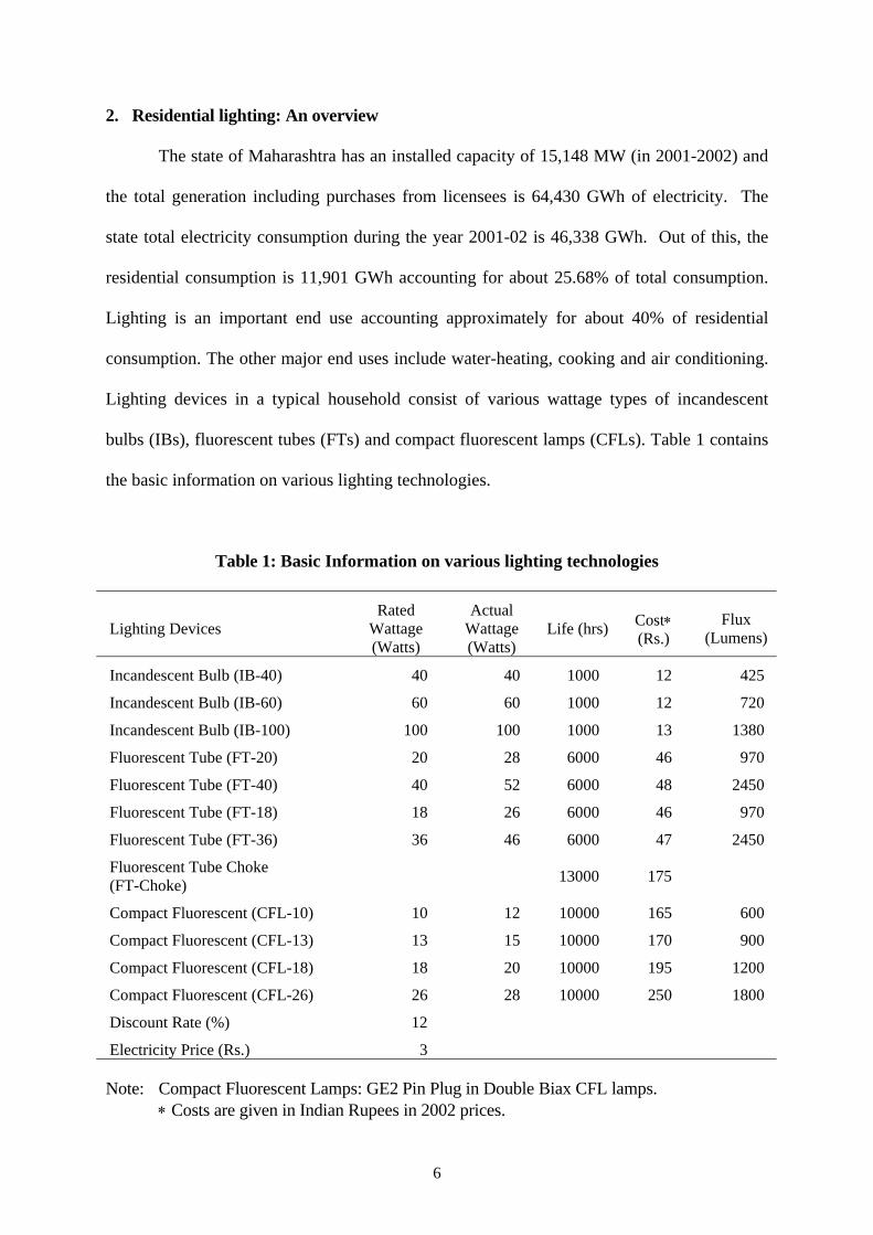
2. Residential lighting: An overview

The state of Maharashtra has an installed capacity of 15,148 MW (in 2001-2002) and

the total generation including purchases from licensees is 64,430 GWh of electricity. The

state total electricity consumption during the year 2001-02 is 46,338 GWh. Out of this, the

residential consumption is 11,901 GWh accounting for about 25.68% of total consumption.

Lighting is an important end use accounting approximately for about 40% of residential

consumption. The other major end uses include water-heating, cooking and air conditioning.

Lighting devices in a typical household consist of various wattage types of incandescent

bulbs (IBs), fluorescent tubes (FTs) and compact fluorescent lamps (CFLs). Table 1 contains

the basic information on various lighting technologies.

Table 1: Basic Information on various lighting technologies

Lighting Devices Rated

Wattage (Watts)

Actual Wattage (Watts)

Life (hrs) Cost∗ (Rs.)

Flux (Lumens)

Incandescent Bulb (IB-40) 40 40 1000 12 425



Fluorescent Tube (FT-20) 20 28 6000 46 970




Fluorescent Tube Choke (FT-Choke) 13000 175

Compact Fluorescent (CFL-10) 10 12 10000 165 600




Discount Rate (%) 12

Electricity Price (Rs.) 3

Note: Compact Fluorescent Lamps: GE2 Pin Plug in Double Biax CFL lamps. ∗ Costs are given in Indian Rupees in 2002 prices.

6

The number of lighting points in a typical household is assumed to be equal to 10 and

the average hours of usage per day is estimated to be three hours (Reddy, 1995). These usage

hours are arrived at by matching the lighting points with the commonly present rooms in a

typical house and the usage pattern (Levy and Sarnat, 1994). The assumed distribution of

these devices according to various levels of usages (hours per day) is given in Table 2. Also,

the table contains information on the approximate level of lighting (Lumens) required for

these usage hours.

Table 2: Lighting devices/level requirements in a typical household

Lighting Locations

Usage (Hours per day)

Required Lighting Level (Lumens) Number of Devices Required

1 0.5 425 One IB-40 or CFL-10 or equivalent

2 1 425 One IB-40 or CFL-10 or equivalent

3 1.5 720 One IB-60 or FT-20 or CFL-13 or equivalent

4 2 720 One IB-60 or FT-20 or CFL-13 or equivalent

5 3 1800 One IB-40 and IB-100 or two CFL-13 or equivalent

6 4 2400 Two IB-100 or one FT-40 or two CFL-18 or equivalent

7 5 2400 Two IB-100 or one FT-40 or two CFL-18 or equivalent

8 6 1200 One IB-100 or one CFL-18 or equivalent

The lighting requirements and the available technologies are matched to obtain the

feasible replacements of IBs with efficient devices (Table 3). As can be seen from the table,

the shifts suggested do not exactly equal in terms of lighting levels (lumens). This is because,

the shift has been allowed even if the lighting service is higher than the standard one.

7

Table 3: Feasible lighting alternatives

Standard Devices Efficient Devices

Incandescent Bulb (IB-40)

Fluorescent Tube (FT-20)


Compact Fluorescent Lamp (CFL-10)











3. Efficient lighting technologies and the rate of return

The lighting technologies, unlike the common stock options, do not provide direct

returns in monetary terms but provide the service, i.e., light output from the lamps. These are

indirect returns in the form of cost savings in relation to inefficient devices. The lighting

technologies considered for the present portfolio posses approximately the same amount of

light output and the differences are only in energy input and the cost of these devices. That is,

the return based on the light output is the same for all the types of lighting technologies that are

studied here. Therefore, the monetary returns are the costs saved on account of reduced energy

input required for obtaining the same level of energy service/lighting when compared to the

existing inefficient lighting device. Since these returns are in relation to the inefficient devices,

we term them as relative returns.

In the present study, the relative returns have been calculated for the feasible efficient

replacements by keeping the returns from IB as constant at zero. This concept of relative

returns and the risk involved are shown graphically in Figure 1. According to the figure the

origin O has been moved to new origin On to exclude the return and risk from the light output

8

of IBs. Thus, return RIBs and risk σIBs for IBs are equal to zero. The values for RFTs and σ FTs for

FTs and RCFLs and σ CFLs for CFLs are obtained in relation to IBs.

Figure 1: Relative return and Risk

O σIBs

RIBs

RCFLs CFLs

FTs

IBs

On σFTs σCFLs

RFTs

Risk (%)

Expected Return (%)

Note: R = Returns; O = Origin, On = New Origin; σ = Risk

4. Expected rates of return on investment

The relative returns from assets of lighting technologies do not remain constant since

the purchase price of the devices and electricity tariff change over the years. The returns also

can vary with these parameters. Therefore, it is not proper to use just the estimated returns or

rates of return for any given year to arrive at some conclusions. For making any reasonable

choice of portfolio, it is required to estimate the expected returns from various devices

considering variations in the returns across the years. For this, the most commonly used

technique is to use the average of returns over the years. In the present analysis, only the

9

variations likely to be caused due to changes in purchase price of lighting devices and the

electricity are included.

Since it is very difficult to obtain the cost of lighting devices for different years, the

wholesale price index is used as a proxy for changes in device costs while electricity price

index is used to estimate the annual electricity prices. The following formulae have been used

to obtain these estimates by using the purchase cost of lighting devices and the electricity price

in 2001 as reference data. The purchase cost of device is given by

Cit = Ci * (P.It/P.I) (1)

Similarly for electricity price,

pt = p * (E.Pt/E.P) (2)

With above assumptions, the annual rates of return for feasible alternatives of IB

replacements have been estimated as follows.

4.1 Annual cost of using the lighting device

To estimate the annual cost, the discounted cash flow (DCF) technique is used. The

factors that are considered include the cost of the devices, their life, electricity price, electricity

consumption and the discount rate using the following equation:

Ait = [Cit/PV(1, d, n)] + Eit * pt (3)

N

PV(1, d, n) = Σ 1/(1+d)n (4) n=1 The annual costs of the devices have been estimated by using the basic data given in

Table 1. In addition, the data on the wholesale price indices and electricity price indices from

1971-72 to 2001-02 are used for estimating the year-wise cost of devices and electricity prices.

The electricity consumption is estimated assuming five hours of daily usage.

10

4.2 Estimation of annual rate of return on investment

As mentioned earlier, the returns are relative returns, which are the differential costs

(cost saved) between the original IBs and the replaced FTs and CFLs. Thus, the relative annual

return for a given type of replaced FT is the difference between its annual cost of utilisation and

that of original IB. The annual rate of return is the percentage return over the total cost incurred

in utilising the original device.

4.3 Estimation of expected annual rate of return on investment

Generally, the expected annual rate of return on any investment is estimated by

averaging the annual rates of return of different years. The standard deviation of this series

gives the associated risk (Levy and Sarnat, 1994). However, this method cannot be used in

cases of FT and CFL since the annual rates of return show an increasing trend. Hence, as a

second best approximation, regression analysis has been carried out using time as

independent variable and actual rates of return as dependent variable. The regression

equations obtained for annual rates of return of FT and CFL are given in Table 4. In the table,

Rt is the expected rate of annual returns for any given year `t’. The high R2 and t-values show

that the obtained regression equations and the coefficients are highly significant. Thus, the

returns estimated by the regression equations give the expected future returns from investing

in assets of lighting technologies. The risks associated with these investments, which include

the fluctuations in the energy carrier prices and the device costs, are given by the standard

error of their estimates. Other uncertainties such as life of the device, discount rates are not

considered in this model but they have been analysed as part of sensitivity analysis.

To compare the investments in lighting technologies, we have used the stock market

option. The Reserve Bank of India (RBI) share price index has been used for estimating the

average annual rates of return from the stock market. The return is the percentage change in

share price index from year to year (1971-72 to 2001-02). However, in the case of annual

11

rates of return from the stock market no clear trend could be observed from the data.

Therefore, the average of the annual rates of return is used as the best approximation for the

future expected returns.

Table 4: Long term expected annual returns of various alternatives of IB

replacements

Feasible Alternatives Regression Equation Expected Annual Returns for

2001-02 (%) Risk∗ (%)

IB-40 → FT-20 Rt = -0.222 + 0.479 * t

R2 = 0.841, t-value = 12.168

14.14 1.865

IB-40 → FT-18 Rt = 3.849 + 0.493 * t

R2 = 0.841, t-value = 12.168

18.65 1.922

IB-40 → CFL-10 Rt = 42.331 + 0.470 * t

R2 = 0.841, t-value = 12.168

55.48 1.707

IB-60 -→ FT-20 Rt = 28.847 + 0.401 * t

R2 = 0.839, t-value = 12.102

40.88 1.571

IB-60 → FT-18 Rt = 31.742 + 0.408 * t

R2 = 0.839, t-value = 12.102

43.99 1.599

IB-60 → CFL-10 Rt = 59.078 + 0.343 * t

R2 = 0.839, t-value = 12.102

69.36 1.342

IB-60 → CFL-13 Rt = 54.022 + 0.344 * t

R2 = 0.839, t-value = 12.102

64.33 1.346

IB-100 → FT-40 Rt = 33.166 + 0.249 * t

R2 = 0.838, t-value = 12.048

40.63 0.979

IB-100 → FT-36 Rt = 38.762 + 0.256 * t

R2 = 0.838, t-value = 12.048

46.43 1.006

IB-100 → CFL-18 Rt = 64.320 + 0.263 * t

R2 = 0.838, t-value = 12.048

72.21 1.035

IB-100 → CFL-26 Rt = 52.109 + 0.334 * t

R2 = 0.838, t-value = 12.048

62.12 1.313

Stock Market 13.62 20.89 Note: The estimates are based on a five hours per day usage ∗The Risk accounted here is the possibility of suffering financial loss due to fluctuation in the price of

electricity and device costs.

12

The estimated expected returns and risks (standard deviations) from the feasible alternatives

of FTs, CFLs and the stock market respectively for the year 2001-02 (reference year for

further analysis) are presented in Table 4. From these estimates, it is clear that replacement

of 100 Watt IB with 18 Watt CFL gives the highest return. It may be observed from the table

that the expected returns from CFL variants range from 55.48% to 72.21% with associated

risks ranging from 1.03% to 1.71% compared to FT variants where the range of expected

rates of return is 14.14% - 46.43 % with risk varying from 0.98% to 1.92%. This shows that

the rates of return from CFL replacements are significantly higher than FTs at comparable

risk levels. Comparatively, the stock market provides an average rate of return of 13.62%

with a risk level of 20.89%. One can expect a very high rate of return from both FTs and

CFLs compared to that in stock market (i.e., on the basis of average returns) at a relatively

very low risk. In other words, the results indicate that investing in efficient lighting retrofits is

highly profitable and reliable to an individual compared to investing in the stock market. One

draw back with this option is that the investments in lighting technologies are limited by the

number of lighting devices required in a given household. However, this kind of limitation is

not applicable to the stock market option where an individual can continue to investing in it.

4.4 Annual rates of return for various usage patterns

The annual rates of return are estimated for all the feasible alternatives (at different

usage hours) using the same methodology as explained earlier. Table 5 contains the estimated

annualised capital as well as electricity costs for various devices at different levels of usage.

It may be observed that, on an average, annualised capital costs are the lowest in the case of

IB variants compared to FTs and CFLs. CFL variants are the most capital intensive of the

three types of competing technologies.

13

14

Table 5: Estimated annualised capital and energy costs (Rs.) of lighting devices for different usage hours

IB-40 IB-60 IB-100 FT-20 FT-36 FT-40 FT-18 CFL-10 CFL-13 CFL-18 CFL-26 Hours per day

Cap-ital Energy Cap-

ital Energy Cap-ital Energy Cap-




ital Energy Cap-ital Energy

0.5 3.1 21.9 3.1 32.9 3.4 54.8 26.7 15.3 26.8 25.2 26.9 28.5 26.7 14.2 19.8 6.6 20.4 8.2 23.4 11.0 30.1 15.3

1.0 5.4 43.8 5.4 65.7 5.8 109.5 27.9 30.7 28.1 50.4 28.2 56.9 27.9 28.5 20.7 13.1 21.4 16.4 24.5 21.9 31.4 30.7

1.5 7.7 65.7 7.7 98.6 8.3 164.3 30.3 46.0 30.5 75.6 30.6 85.4 30.3 42.7 22.7 19.7 23.3 24.6 26.8 32.9 34.3 46.0

2.0 10.0 87.6 10.0 131.4 10.8 219.0 33.3 61.3 33.5 100.7 33.7 113.9 33.3 56.9 25.1 26.3 25.9 32.9 29.7 43.8 38.1 61.3

3.0 14.6 131.4 14.6 197.1 15.9 328.5 40.3 92.0 40.6 151.1 40.8 170.8 40.3 85.4 30.7 39.4 31.6 49.3 36.3 65.7 46.5 92.0

4.0 19.3 175.2 19.3 262.8 20.9 438.0 47.9 122.6 48.2 201.5 48.5 227.8 47.9 113.9 36.7 52.6 37.8 65.7 43.3 87.6 55.6 122.6

5.0 23.9 219.0 23.9 328.5 25.9 547.5 55.7 153.3 56.0 251.9 56.4 284.7 55.7 142.4 42.8 65.7 44.1 82.1 50.6 109.5 64.9 153.3

6.0 28.6 262.8 28.6 394.2 30.9 657.0 63.6 184.0 64.0 302.2 64.5 341.6 63.6 170.8 49.0 78.8 50.5 98.6 57.9 131.4 74.3 184.0

Note: Costs are in Indian Rupees (02 prices).

15

The annual cost of utilising these lighting devices is given in Table 6. According to

the table, the annual energy costs are the lowest in the case of CFL variants compared to

those of FTs and IBs. In terms of total annual costs, CFL-10, CFL-13 and CFL-18 fare better

than the variants of FTs and IBs. Only CFL-26 is more expensive compared to IB-40, FT-18

and FT-20. However, it is important to note that all these lighting alternatives provide

different levels of light outputs.

Table 6: Annual cost of utilisation of lighting devices for different usage hours (Rs.) Hours per day IB-40 IB-60 IB-100 FT-20 FT-36 FT-40 FT-18 CFL-10 CFL-13 CFL-18 CFL-26

0.5 25.0 36.0 58.1 42.0 52.0 55.4 40.9 26.4 28.7 34.4 45.41 49.2 71.1 115.3 58.6 78.4 85.1 56.4 33.9 37.8 46.4 62.1

1.5 73.4 106.3 172.6 76.3 106.0 116.0 73.0 42.4 48.0 59.6 80.32 97.6 141.4 229.8 94.6 134.3 147.6 90.3 51.4 58.7 73.5 99.43 146.0 211.7 344.4 132.3 191.7 211.7 125.7 70.1 80.9 102.0 138.54 194.5 282.1 458.9 170.5 249.7 276.3 161.8 89.2 103.5 130.9 178.25 242.9 352.4 573.4 209.0 307.9 341.1 198.0 108.5 126.2 160.1 218.26 291.4 422.8 687.9 247.5 366.2 406.1 234.4 127.9 149.0 189.3 258.2

Note: Costs are in Indian Rupees (in 2005 prices).

The annual rates of return are estimated for different feasible alternatives of

replacements at different usage hours (Table 7). It may be observed that the replacement of 100

Watts IB with 18 Watts CFL gives a maximum return of 72.5% at six hours usage. Among the

other alternatives, shift from IB-100 to CFL-18 provides the highest returns for all the usage

hours. Based on the rate of return criteria this may seem to be the obvious and only choice in

the portfolio of devices. However, from the point of technical feasibility, this may not be the

only optimal choice. Because the lighting levels required at various usage hours are different

and also the light output levels are different for various lighting alternatives. Discussions on

this issue are made in subsequent sections.

16

Table 7: Annual rates of return for different usage hours for feasible alternatives of IB replacements (%)

Hours per day

Feasible Alternatives 0.5 1 1.5 2 3 4 5 6

IB-40 → FT-20 -67.9 -19.1 -3.9 3.0 9.4 12.3 14.0 15.0 IB-40 → FT-18 -63.5 -14.6 0.6 7.5 13.9 16.8 18.5 19.6 IB-40 → CFL-10 -5.6 31.2 42.3 47.3 52.0 54.1 55.3 56.1 IB-60 → FT-20 -16.8 17.6 28.2 33.1 37.5 39.6 40.7 41.4 IB-60 → FT-18 -13.7 20.7 31.3 36.2 40.6 42.7 43.8 44.6 IB-60 → CFL-10 26.6 52.4 60.1 63.7 66.9 68.4 69.2 69.8 IB-60 → CFL-13 20.3 46.9 54.8 58.5 61.8 63.3 64.2 64.7 IB-100 → FT-40 4.7 26.2 32.8 35.8 38.5 69.9 70.3 41.0 IB-100 → FT-36 10.6 32.0 38.6 41.6 44.3 72.8 73.2 46.8 IB-100 → CFL-18 40.8 59.8 65.5 68.0 70.4 71.5 72.1 72.5 IB-100 → CFL-26 21.9 46.2 53.5 56.8 59.8 70.9 71.5 62.5

5. Optimal portfolio of lighting technologies

The typical household that is considered for this study has a choice of 11 different

lighting devices for 10 lighting points. A Mixed Integer Programming (MIP) model is

developed to make an optimal selection among the alternatives considering both the

economic as well as technical feasibility criteria. Economic feasibility is measured through

the returns that could be obtained through an efficient replacement where as the technical

feasibility is measured in terms of lighting level demanded and the potential of a given device

to provide that level of lighting. In cases where a single device is unable to provide sufficient

lighting, a combination of devices is used. A mixed integer programming model is used and

the model solution gives the optimal portfolio of lighting technologies.

The objective function for the model is to maximize the annual returns by replacing the

standard device with an efficient one.

I,J K I,J K

Max Z = Σ Σ (Cik – Cjk) * Ni→j,k - Σ Σ OCi→j,k (5) i,j = 1 k=1 i,j = 1 k=1

17

The constraints are as follows:

i. Number of lighting devices required for a given usage hour

The total number of lighting devices in a given room should be at least equal to the

given number, which is being used for a given duration in hours.

I,J

Σ Ni→j,k ≥ Nk for all k (6) i,j = 1

ii. Total number of lighting devices for a typical house hold

The total number of lighting devices in a given household should not be more than the

required number.

I,J K

Σ Σ Ni→j,k ≤ N (7) i,j = 1 k=1

iii. Demand for the level of lighting

The level of lighting (Flux measured in Lumens) in a given room should be at least

equal to the prescribed level.

I,J

Σ Li→j * Ni→j,k ≥ Lk for all k (8) i,j = 1

iv. Opportunity cost of using inappropriate lighting device

The consumer can have a flexibility of choosing a higher wattage lighting device to

get more lighting than the prescribed level. However, there are extra costs involved in terms

of higher capital and energy costs that need to be incurred to have this facility. The difference

in costs between the higher wattage device and the prescribed device is considered here as the

opportunity cost.

ECi→j * Ni→j,k = OCi→j for all i, j and k (9)

18

v. Non-negativity Constraints

All variables ≥ 0

5.1 Estimation of portfolio returns and risk

The portfolio returns are calculated as follows:

m

Rp = ∑ Ri * Pi (10) i=1 The variance associated with the portfolio is calculated as follows:

m m

σp2 = ∑ ∑ Pi * Pj * σ i,j (11)

i=1 j=1

The portfolio risk (standard deviation) is given by the square root of the variance.

5.2 Optimal portfolio of lighting technologies

The solution to the mixed integer programming model is the optimal portfolio

containing one 40 Watt IB, two 36 Watt FT, one 10 Watt CFL, four 13 Watt CFLs and one 18

Watt CFL (Table 8).

Table 8: Optimal Portfolio of lighting devices

Lighting Devices

Hours per day

Number Required

Investment (Rs.)

Annual Returns (Rs.)

Estimated Returns (%)

Expected Returns (%)

Risk (%)

Replacement Cycle (Yrs.)

IB-40 0.5 1 12 0.00 0.00 0.00 0.00 5.48

CFL-10 1 1 165 15.33 31.15 31.49 4.41 2.74 CFL-13 1.5 1 170 58.27 54.84 55.10 2.48 10.96 CFL-13 2 1 170 82.68 58.47 58.69 2.04 8.22 CFL-13 3 2 340 328.58 67.00 67.17 1.46 9.13 FT- 36 4 1 222 668.10 72.80 72.86 0.55 4.11 FT- 36 5 1 222 838.93 73.15 73.22 0.50 3.29 CFL-18 6 1 195 498.61 72.48 72.60 0.98 4.57 Total 9 1496 2490.50 Note: Indian Rupees (in 2002 prices)

19

The initial investment required to have this portfolio is Rs. 1,496 and the annual returns are Rs.

2,490. This means that the expected rate of return on investment is about 166% with a payback

period of 0.6 year. Within the portfolio, FT-36 provides the highest returns at five hours usage.

Even though, IB provides no returns, it is included in the portfolio since the replacements are

neither technically feasible nor provide positive returns at that usage level. The estimated

portfolio return is 62.65%. The long-term expected portfolio return (estimated using the

regression equations) is 62.81% with an associated risk level of 0.71%. Compared to this, the

long-term investments in stock market provide only 13.62% returns with a very high risk of

20.89% (Table 9).

Table 9: Summary results of portfolio of lighting devices

Return on Investment (%) 166.48

Payback Period (Years) 0.60

Estimated Portfolio Returns (%) 62.65

Expected Portfolio Returns (%) 62.81

Portfolio risk (%) 0.71

Indian Stock Market Returns∗ (%) 13.62

Indian Stock Market Risk (%) 20.89

∗average for the years 1971-72 to 2001-05.

Figure 2 presents a comparison of estimated annual rates of return (actual and expected)

from the replaced FT-36 and CFL-18 for five hours usage with those from the stock market for

the years 1971-72 to 2001-02. For comparison, the approximate matching in terms of light

output is obtained by considering the combination of 60 and 100 Watt IBs to be equal to one 36

Watt FT or two 18 Watt CFLs. From the figure one may observe a clear increasing trend in the

cases of returns from FT-36 and CFL-18. Among the two, FT-36 consistently provides a

higher rate of return. In comparison, the stock market returns show no particular trend and the

-30.000

-20.000

-10.000

0.000

10.000

20.000

30.000

40.000

50.000

60.000

70.000

80.000

1 5 9 13 17 21 25 29

Years

Rat

e of

Ret

urns

(%)

IB-->CFL (Estimated) IB-->CFL (Expected)IB-->FT (Estimated) IB-->FT (Expected)Stock Market (Estimated) Stock Market (Expected)

Figure 2. Annual Returns from retrofitted efficient lighting devices and stock market.

20

21

fluctuations are very high. This clearly shows that in the long run, investments in efficient

lighting alternatives provide safe and high returns compared to the stock market.

6. Perspectives - Optimal And Other Scenarios

6.1 Customer Perspective

Implementation of efficient options reduces the energy bills of the consumer

significantly. These savings by customers are determined by using a rate module that computes

customers' bills for the standard technology and after the use of efficient technology (Reddy,

1996). The differences between the two are the savings for customers. In order to compare the

overall performance of the optimal portfolio of lighting technologies (Optimal Case Scenario

- OCS), two scenarios have been developed. The first one (Worst Case Scenario - WCS)

considers the portfolio of only IBs to meet the demand for lighting and the second one, being

the Medium Case Scenario (MCS) considers a possible mix of IBs and FTs. The results of

this analysis are presented in Table 10.

22

Table 10: Optimal and probable portfolios of lighting in the residential sector of Maharashtra - Scenario results

Worst Case Scenario (WCS) Medium Case Scenario (MCS) Optimal Case Scenario (OCS)

Devices Capital Cost (Rs.)

Energy Cost (Rs.)

Energy (kWh) Devices Capital

Cost (Rs.)Energy Cost (Rs.)

Energy (kWh) Devices Capital

Cost Rs.) Energy Cost (Rs.)

Energy (kWh)

Hours per Day

IB-40 12 21.9 7.3 IB-40 12 21.9 7.3 IB-40 12 21.9 7.3 0.5

IB-40 12 43.8 14.6 IB-40 12 43.8 14.6 CFL-10 165 13.1 4.4 1 IB-60 12 98.6 32.9 IB-60 12 98.6 32.9 CFL-13 170 24.6 8.2 1.5 IB-60 12 131.4 43.8 IB-60 12 131.4 43.8 CFL-13 170 32.9 11.0 2 IB-(100+40) 25 459.9 153.3 IB-(100+40) 25 459.9 153.3 CFL-13 (two) 340 98.6 32.9 3 IB-100 26 876.0 292.0 FT-Tube-40 223 227.8 75.9 FT-Tube-36 222 201.5 67.2 4 IB-100 26 1095.0 365.0 FT-Tube-40 223 284.7 94.9 FT-Tube-36 222 251.9 84.0 5 IB-100 13 657.0 219.0 FT-Tube-40 223 341.6 113.9 CFL-18 195 131.4 43.8 6 Total 138 3383.6 1127.9 Total 742 1609.7 536.6 Total 1496 775.8 258.6

23

According to the table, in terms of investment (total purchase cost of the devices) by

the household, the requirement in WCS is Rs. 138 and for MCS it is Rs. 742 compared to Rs.

1,496 in the Optimal Case Scenario (OCS). However, in terms of annual energy costs, the

cheapest alternative is provided by OCS with Rs. 776 compared to Rs. 1,610 for MCS and

Rs. 3,384 for WCS. To find out the overall costs and benefits, the results obtained for a

typical household is extended to the total residential sector of Maharashtra state (Table 11).

Table 11: Scenario Results for the Residential Sector of Maharashtra State (2001-02)

Domestic Consumers (No.) 9258154

Annual Consumption (GWh) 11901

Domestic Consumers with 10 lighting points (No.) 1851631

WCS - Consumption (GWh) 2088.36

MCS - Consumption (GWh) 993.49

OCS - Consumption (GWh) 478.84

Total Investment for OCS (Rs. Million) 2770.04

Here we have assumed that, out of a total of 9.26 Million domestic consumers, only

20% will have lighting points equal to 10. Thus the estimates made here for the total

residential sector are only for these consumers. The annual energy savings that could be

achieved by implementing OCS are about 1,609 GWh compared to WCS and about 514

GWh compared to MCS. This results in a cost savings of Rs. 3,129 Million and Rs. 1,029

Millions respectively at an average electricity price of Rs. 3.0/kWh. From the table it may be

observed that the payback periods of around 0.8 and 1.36 years are quite attractive for a shift

from either WCS or MCS to OCS (Table 12).

24

Table 12: Savings of OCS compared to WCS and MCS

WCS MCS

Energy saved (GWh) 1609.53 514.66

Cost of Energy saved (Rs. Million) 3129.05 1029.31

Additional Investment (Rs. Million) 2514.51 1396.13

Payback Period (Years) 0.78 1.36

Peak Demand Saved (MW) 882 282

Cost of Capacity Avoided (Rs. Million) 35277.27 11280.14

6.2 Power Utility Perspective

The average unit cost of electricity to the utility for sales to the consumer is calculated by

dividing the total annual revenue requirement by the total annual generation. If the avoided

costs associated with efficient technologies result in a decrease in average costs without

increasing costs elsewhere in the system, the modification is desirable. The costs for various

lighting technologies are compared with the average cost to the Maharashtra State Electricity

Board (MSEB), which is Rs.2.00/kWh for the year 2001-02. Table 13 gives the estimated unit

costs of energy saved for various devices in the optimal portfolio compared to the WCS and

MCS portfolios. The unit costs vary from a low of Rs. 0.0/kWh (actually negative costs) to Rs.

1.50/kWh while the average being Rs. 0.13/kWh for WCS to OCS and Rs. 0.26/kWh for MCS

to OCS shifts. These values indicate that the costs of efficient lighting options are significantly

lower than the MSEB’s average cost of generation. If the portfolio suggested by the OCS is

implemented, the utility saves money on investments required for new capacity additions as well

as costs of fuel for power generation. The total cost of energy saved due to OCS portfolio

works out to about Rs. 3,129 Million and Rs. 1,029 Million respectively compared to WCS

and MCS (at long run marginal cost of Rs. 2.00/kWh and without considering T&D system

costs and loss component). Even with the lowest estimate, the peak demand saved works out

25

to about 882 MW compared to WCS and 282 MW compared to MCS. This results in cost of

capacity avoided equivalent of Rs. 35,277 Million and Rs. 11,280 Million respectively

compared to WCS and MCS. These savings are very significant.

Table 13: Unit Cost of Energy Saved (Rs/kWh)

Energy Saved (kWh)

Incremental Cost (Rs.)

Unit Cost of Energy Saved (Rs./kWh) Devices

WCS to OCS

MCS to OCS

WCS to OCS

MCS to OCS

WCS to OCS

MCS to OCS

IB-40 0.0 0.0 0 0 --- ---

CFL-10 10.2 10.2 15.33 15.33 1.50 1.50

CFL-13 24.6 24.6 15.64 15.64 0.63 0.63

CFL-13 32.9 32.9 15.87 15.87 0.48 0.48

CFL-13 (two) 120.5 120.5 32.77 32.77 0.27 0.27

FT-36 224.8 8.8 6.42 -0.32 0.03 -0.04

FT-36 281.1 11.0 4.22 -0.39 0.02 -0.04

CFL-18 175.2 70.1 26.99 -6.54 0.15 -0.09

Total 869.2 277.9 117.25 72.36 0.13 0.26

The preceding results indicate that investments in efficient lighting technologies would

reduce the need to construct new power plants. If these options is integrated into the supply-side

process, the investment plans drafted by MSEB to meet anticipated loads will be properly

altered.

7. Sensitivity analysis

In the previous analyses, the estimated risks associated with efficient lighting

alternatives accounted only the variations in rates of return caused by the fluctuations in the

cost of the devices and the price of electricity. In case of physical assets, unlike stocks, there are

other parameters, which determine the level of returns. In our analysis, we have used some such

26

parameters with assumed or actual values for estimating the relative annual returns from the

usage of FTs and CFLs. Any changes in the values of these parameters will have direct impact

on the estimated values of annual returns. For this, a sensitivity analysis is performed to study

the impact of changes in these parameters on the annual returns obtainable from the retrofitting

suggested by the optimal portfolio. This analysis is limited to assessing the sensitiveness of a

given parameter (by making the changes in its value) on the value of rate of return. As

mentioned earlier, the matching of devices is made based on the light output and the choices are

IB-(60+100) to be replaced either by one FT-36 or two CFL-18. Five hours of usage per day is

assumed for this analysis.

7.1 Effect of change in electricity price on annual returns

Figure 3 gives the estimates of annual returns from IB-(60+100) → FT-36 and IB-

(60+100) → CFL-(18*2) replacements for different changes in the electricity prices. It may be

observed from the figure that the replacements provide positive returns and increase with the

50.00

55.00

60.00

65.00

70.00

1 2 3 4 5 6 7

Electricity Price (Rs./kWh)

Ann

ual r

etur

ns (%

)

IB-(60+100)-->CFL-(18*2) IB-(60+100)-->FT-36

Figure 3. Effect of change in electricity price on annual returns.

increase in energy price while tending towards saturation. Beyond the price of Rs. 6.00/kWh,

CFL-18 gives more returns compared to FT-36.

27

40.00

45.00

50.00

55.00

60.00

65.00

70.00

100 200 300 400 500 600

Price in Rupees

Ann

ual r

etur

ns (%

)

IB-(60+100)-->CFL-(18*2) IB-(60+100)-->FT-36

Figure 4: Effect of change in the price of CFL on annual returns

7.2 Effect of change in the cost of CFLs on annual returns

The high cost of CFLs has significant influence on the annual rate of return. The cost

of CFLs used to be quite high in India because of high customs duty and low sales volume.

However, with the setting up of manufacturing facilities within the country and sales level

going up, the prices have declined significantly. Figure 4 clearly shows that, the returns from

CFL-18 are more than that from FT-36 if the price of CFL-18 is below Rs. 175 (Rs. 350 for

two CFLs). 28

-30.00

-20.00

-10.00

0.00

10.00

20.00

30.00

40.00

50.00

60.00

70.00

80.00

0 2500 5000 7500 10000 12500 15000

Life in hours

Ann

ual r

etur

ns (%

)

IB-(60+100)-->CFL-(18*2) IB-(60+100)-->FT-36

Figure 5. Effect of change in the life of lighting devices on annual returns

7.3 Effect of change in the life of CFLs on annual returns

The CFLs are designed to work in the stable range of voltage. However, in India, the

fluctuations vary from 190V - 260V. Despite their design to cope with the fluctuations, the

survival of CFLs have not been adequately tested in the field. Lab tests in India have reported

that the life of CFL is about 10,000 hours. It may be observed (Figure 5) that shifting of IB-

(60+100) to CFL-(18*2) starts providing positive returns once the life exceeds 1,300 hours.

29

However, in comparison, FT-36 gives higher returns than CFL-18 and they appear to converge

as lifespan increases.

-80.00

-60.00

-40.00

-20.00

0.00

20.00

40.00

60.00

80.00

0 2 4 6 8 10

Hours per day

Ann

ual r

etur

ns (%

)

IB-(60+100)-->CFL-(18*2) IB-(60+100)-->FT-36

Figure 6. Effect of change in daily hours of usage on annual returns

7.4 Effect of change in daily hours of usage on annual returns

Another important parameter, which affects the annual returns, is the daily hours of

usage of lighting devices. From Figure 6, it can be observed that one can expect positive returns

30

58.00

60.00

62.00

64.00

66.00

68.00

70.00

0 5 10 15 20 25 30

Discount rates (%)

Ann

ual r

etur

ns (%

)

IB-(60+100)-->CFL-(18*2) IB-(60+100)-->FT-36

Figure 7. Effect of change in discount rates on annual returns

from FT-36 and CFL-18 if daily usage hours are more than 0.2 and 0.4 respectively. With the

present level of device costs and electricity prices, the returns from FT-36 always exceed that of

CFL-18.

7.5 Effect of change in discount rates on annual returns

For estimating the relative annual returns we have used a discount rate of 12 per cent.

Any change in this value will influence changes in annual returns. This is being reflected in

31

32

Figure 7, which clearly shows that there is a strong relationship between annual returns and the

discount rates. A decline in annual returns can be observed with the increase in discount rates.

A high discount rate indicates that the present value of costs is very high compared to future

benefits (or inflows). The decline in returns from IB-(60+100) shift to CFL-18 is more rapid

then that from shift of IB-(60+100) to FT-36 since CFL has a high initial cost.

6 Conclusions

This paper attempts to construct an optimal portfolio of lighting technologies for a

typical household in the State of Maharashtra, India. Initially, 11 feasible alternatives of FT and

CFL for the replacements of inefficient IBs were identified. The relative annual rates of return

for these alternatives are estimated from 1971-72 to 2001-02. Using regression models, the long

term expected rates of return and the associated risks are estimated which are compared to the

average stock market returns and risks. A mixed integer-programming model has been

developed to determine an optimal portfolio of the alternatives. A sensitivity analysis is

performed to study the effects of changes in various parameters on the rates of return from the

efficient alternatives of the portfolio. Finally, a comparison is made of the optimal scenario

with two probable scenarios and the results are extended to estimate the cost and benefits that

could accrue to the residential sector of Maharashtra state and the society as a whole.

The comparison of three lighting technologies indicates that, though expensive, the

CFLs are a quite attractive proposition in terms of returns compared to IBs while the FT

variants are quite close to CFLs. The advantages with FTs are that they provide the returns at

lower risk levels compared to those of CFLs. With the expected increase in electricity prices

and the declining CFL costs makes them highly attractive investment proposals. The results

also show that the optimal lighting portfolio provides a far higher return at a lower risk

33

compared to the stock market. The overall results indicate a substantial savings both in terms

of energy and peak demand for the state.

Nomenclature

Cit = Purchase cost of device i in the year t

Ci = Cost of device i in reference year (i.e., 2001-02)

P.It = Wholesale price index value in the year t

P.I = Wholesale price index in the reference year (2001-02)

pt = Electricity price in the year t

p = Electricity price in the reference year (i.e., 2001-02)

E.Pt = Electricity price index value in the year t

E.P = Electricity price index in the reference year (2001-02)

Ai = Annual cost of utilising the device type i

d = Discount Rate in per cent

n = Life of the Device in years

Ei = Electricity consumption per year by the device i

PV = Present Value

i = Type of original lighting device, i = 1, 2, …., I

j = Type of replaced lighting device, j = 1, 2, …., J

k = Type of usage hours, k = 1, 2, ….., K

Cik = Annual cost of utilisation of original device `i’ for `k’th usage hours

Cjk = Annual cost of utilisation of replaced device `j’ for `k’th usage hours

Ni→j,k = Number of replaced lighting devices of type `j’ used for `k’th usage hours

OCi→j,k = Opportunity cost of not using the appropriate device for `k’th usage hours

Nk = Minimum number of lighting devices for `k’th usage hours

34

N = Maximum number of lighting devices in a given household

Li→j = Lighting levels (Flux in Lumens) given by the lighting device

Lk = Minimum lighting level required where the duration of usage type is `k’

ECi→j = Extra cost needs to be incurred for adopting higher wattage device

OCi→j = Opportunity cost of using inappropriate device

Rp = Portfolio rate of return

Ri = Expected rate of return on asset i

Pi = Proportion of asset i in total investment

m = Total number of assets in the portfolio

σp2 = Portfolio variance

Pj = Proportion of asset j in total investment

σ i,j = Covariance

σ i,i/σi2 = Variance

References

Dutt, G.S. (1994) ‘Illumination and sustainable development: part I’, Energy for Sustainable

Development, Vol. 1, No. 2, pp.21-33.

Gadgil, A.J. and Jannuzzi, G.D.M. (1994) ‘Conservation potential of compact fluorescent lamps

in India and Brazil’, Energy Policy, Vol. 19, No. 5, pp.449-463.

Johnson, B.E. (1994) ‘Modeling energy technology choices’, Energy Policy, Vol. 22, No. 10,

pp.877-883.

Levy, H. and Sarnat, M. (1994) Capital investment and financial decisions. London: Prentice

Hall.

Metcaff, G.E. (1994) ‘Economics and Rational Conservation Policy’, Energy Policy, Vol. 22,

No. 10, pp.819-825.

Sutherland, R.J. (1986) ‘A Portfolio Analysis Model of the Demand for Nuclear Power Plants’,

Energy Economics, Vol. 8, No. 4, pp.218-226.

Sutherland, R.J. (1991) ‘Market barriers to energy-efficiency investments’, The Energy Journal,

Vol. 12, No. 3, pp.15-34.

Sudhakara Reddy B. (1995) ‘Appliance Electricity Consumption in the Residential Sector: An

Economic Approach’, Energy Sources, Vol. 17, No. 2, pp.179-193.

Sudhakara, Reddy B. (1996) ‘Consumer Discount Rates and Energy Carrier Choices in Urban

Households’, International Journal of Energy Research, Vol. 20, No. 4, pp.187-195.

Sudhakara Reddy, B. (1996) ‘Economic evaluation of Demand Side Management Programmes’,

Energy- The International Journal, Vol. 21, No. 6, pp.473-482.

35

technology portfolio analysis for residential … portfolio analysis for residential lighting ......

Documents