technical report – train benchmark · 3.2.1 emf-based tools ... from efficiently storing or...
TRANSCRIPT

Project Number 611125
Technical Report – Train Benchmark
Version 0.91 August 2014
Draft
Public Distribution
BME
Project Partners: ARMINES, Autonomous University of Madrid, BME, IKERLAN, Soft-Maint,SOFTEAM, The Open Group, UNINOVA, University of York
Every effort has been made to ensure that all statements and information contained herein are accurate, howeverthe Project Partners accept no liability for any error or omission in the same.
© 2014 Copyright in this document remains vested in the MONDO Project Partners.

Technical Report – Train Benchmark
Project Partner Contact Information
ARMINES Autonomous University of MadridMassimo Tisi Juan de LaraRue Alfred Kastler 4 Calle Einstein 344070 Nantes Cedex, France 28049 Madrid, SpainTel: +33 2 51 85 82 09 Tel: +34 91 497 22 77E-mail: [email protected] E-mail: [email protected]
BME IKERLANDaniel Varro Salvador TrujilloMagyar Tudosok korutja 2 Paseo J.M. Arizmendiarrieta 21117 Budapest, Hungary 20500 Mondragon, SpainTel: +36 146 33598 Tel: +34 943 712 400E-mail: [email protected] E-mail: [email protected]
Soft-Maint SOFTEAMVincent Hanniet Alessandra BagnatoRue du Chateau de L’Eraudiere 4 Avenue Victor Hugo 2144300 Nantes, France 75016 Paris, FranceTel: +33 149 931 345 Tel: +33 1 30 12 16 60E-mail: [email protected] E-mail: [email protected]
The Open Group UNINOVAScott Hansen Pedro MalóAvenue du Parc de Woluwe 56 Campus da FCT/UNL, Monte de Caparica1160 Brussels, Belgium 2829-516 Caparica, PortugalTel: +32 2 675 1136 Tel: +351 212 947883E-mail: [email protected] E-mail: [email protected]
University of YorkDimitris KolovosDeramore LaneYork YO10 5GH, United KingdomTel: +44 1904 32516E-mail: [email protected]
Page ii Version 0.9Confidentiality: Public Distribution
1 August 2014

Contents
1 Overview 2
1.1 Overview . . . . . . . . . . . . . . . . . . . . . . . . . . . . . . . . . . . . . . . . 2
1.2 Instance Models . . . . . . . . . . . . . . . . . . . . . . . . . . . . . . . . . . . . . 3
1.3 Queries and Transformations . . . . . . . . . . . . . . . . . . . . . . . . . . . . . . 3
1.4 Evaluation of Measurements . . . . . . . . . . . . . . . . . . . . . . . . . . . . . . 4
2 Train Benchmark Technical Specification 5
2.1 Original Version . . . . . . . . . . . . . . . . . . . . . . . . . . . . . . . . . . . . . 5
2.1.1 Phases . . . . . . . . . . . . . . . . . . . . . . . . . . . . . . . . . . . . . . 5
2.1.2 Use Case Scenarios of the Benchmark . . . . . . . . . . . . . . . . . . . . . 6
2.1.3 Metamodel . . . . . . . . . . . . . . . . . . . . . . . . . . . . . . . . . . . 7
2.1.4 Queries . . . . . . . . . . . . . . . . . . . . . . . . . . . . . . . . . . . . . 7
2.1.5 Transformations . . . . . . . . . . . . . . . . . . . . . . . . . . . . . . . . 12
2.1.6 Instance Model Generation . . . . . . . . . . . . . . . . . . . . . . . . . . . 15
2.2 Extended version . . . . . . . . . . . . . . . . . . . . . . . . . . . . . . . . . . . . 16
2.2.1 Overview . . . . . . . . . . . . . . . . . . . . . . . . . . . . . . . . . . . . 17
2.2.2 Metrics . . . . . . . . . . . . . . . . . . . . . . . . . . . . . . . . . . . . . 17
2.2.3 Modified Metamodel . . . . . . . . . . . . . . . . . . . . . . . . . . . . . . 19
2.2.4 Instance Models for the Modified Metamodel . . . . . . . . . . . . . . . . . 19
2.2.5 Benchmark Queries . . . . . . . . . . . . . . . . . . . . . . . . . . . . . . . 21
2.2.6 Complex Analysis . . . . . . . . . . . . . . . . . . . . . . . . . . . . . . . 24
2.3 Implementation architecture . . . . . . . . . . . . . . . . . . . . . . . . . . . . . . 24
2.3.1 Parent module . . . . . . . . . . . . . . . . . . . . . . . . . . . . . . . . . 24
2.3.2 Central modules . . . . . . . . . . . . . . . . . . . . . . . . . . . . . . . . 24
2.3.3 Representation-specific modules . . . . . . . . . . . . . . . . . . . . . . . . 24
iii

Technical Report – Train Benchmark
2.3.4 Generator modules . . . . . . . . . . . . . . . . . . . . . . . . . . . . . . . 26
2.3.5 Benchmark modules . . . . . . . . . . . . . . . . . . . . . . . . . . . . . . 26
2.3.6 4store . . . . . . . . . . . . . . . . . . . . . . . . . . . . . . . . . . . . . . 26
3 Benchmark Results 273.1 Benchmarking Environment . . . . . . . . . . . . . . . . . . . . . . . . . . . . . . 27
3.2 Tools . . . . . . . . . . . . . . . . . . . . . . . . . . . . . . . . . . . . . . . . . . . 27
3.2.1 EMF-based Tools . . . . . . . . . . . . . . . . . . . . . . . . . . . . . . . . 28
3.2.2 RDF-based Tools . . . . . . . . . . . . . . . . . . . . . . . . . . . . . . . . 29
3.2.3 Graph-based Tools . . . . . . . . . . . . . . . . . . . . . . . . . . . . . . . 29
3.2.4 SQL-based Tools . . . . . . . . . . . . . . . . . . . . . . . . . . . . . . . . 30
3.3 Measurement Results for Performance Comparison . . . . . . . . . . . . . . . . . . 30
3.3.1 How to read the charts . . . . . . . . . . . . . . . . . . . . . . . . . . . . . 30
3.3.2 Batch Validation . . . . . . . . . . . . . . . . . . . . . . . . . . . . . . . . 31
3.3.3 Revalidation . . . . . . . . . . . . . . . . . . . . . . . . . . . . . . . . . . 35
3.3.4 Total time . . . . . . . . . . . . . . . . . . . . . . . . . . . . . . . . . . . . 39
3.3.5 Series of Edit times . . . . . . . . . . . . . . . . . . . . . . . . . . . . . . . 43
3.3.6 Series of Incremental Revaliation Times . . . . . . . . . . . . . . . . . . . . 45
3.4 Analysis of results . . . . . . . . . . . . . . . . . . . . . . . . . . . . . . . . . . . . 47
3.4.1 Batch validation . . . . . . . . . . . . . . . . . . . . . . . . . . . . . . . . 47
3.4.2 Incremental revalidation . . . . . . . . . . . . . . . . . . . . . . . . . . . . 48
3.4.3 Highlights of interest . . . . . . . . . . . . . . . . . . . . . . . . . . . . . . 48
3.4.4 Threats to Validity . . . . . . . . . . . . . . . . . . . . . . . . . . . . . . . 49
3.5 Evaluation of Metrics . . . . . . . . . . . . . . . . . . . . . . . . . . . . . . . . . . 50
3.5.1 Method of Analysing Metrics . . . . . . . . . . . . . . . . . . . . . . . . . 50
3.5.2 Metrics Colleration Results . . . . . . . . . . . . . . . . . . . . . . . . . . 51
3.5.3 Threats to Validity . . . . . . . . . . . . . . . . . . . . . . . . . . . . . . . 52
4 Summary 53
A Appendix 54A.1 Rete Networks for the Queries of the Train Benchmark . . . . . . . . . . . . . . . . 54
Page iv Version 0.9Confidentiality: Public Distribution
1 August 2014

Technical Report – Train Benchmark
Document Control
Version Status Date0.1 Document outline 30 November 20130.2 First draft - structure ready 17 January 20140.3 Second draft - incorporation
of ASE material06 March 2014
0.5 Third draft - revised contents 10 March 20140.8 Fourth draft - results
complete, analysis needsrework
10 April 2014
0.9 Fifth draft - complete 1 June 2014
1 August 2014 Version 0.9Confidentiality: Public Distribution
Page v

Executive Summary
The main goal of the Train Benchmark is to measure the execution time of graph-based query pro-cessing tools with particular emphasis on incremental query reevaluation. The execution time ismeasured against models of growing sizes generated by an instance model generator. This way, thescalability of the tools is evaluated. The Train Benchmark also demonstrates other abilities of thetools, including transformation capabilities, conciseness of the query and transformation language,convenience of the API, compatibility with different metamodeling languages and so on. The TrainBenchmark is a general benchmarking framework, that contains a specific benchmark test case setbuilt around a metamodel inspired by railway system design. This test case set also comes with a setof queries and transformation operations.
The current tech report includes information on two variants of the Train Benchmark: the originalversion was described in [31] and describes the incremental well-formedness checking scenario. Theextended version was described in [22] and introduces query and instance model query metrics toquantitatively assess the “difficulty” of various model query-instance model combinations to findthose metrics that are best for predicting the query evaluation time without running the query itself.
The most up-to-date supplementary material is found at https://opensourceprojects.eu/p/mondo/wiki/TrainBenchmark
1
Chapter 1
Overview
Scalability issues in model-driven engineering arise due to the increasing complexity of modelingworkloads. This complexity comes from two main factors: (i) instance model sizes are exhibiting atremendous growth as the complexity of systems-under-design is increasing, (ii) increasing featuresophistication in toolchains, such as complex model validation or transformations.
One of the the most computationally expensive tasks in modeling applications are model queries.While there are a number of existing benchmarks for queries over relational databases [30] or graphstores [13, 27], modeling tool workloads are significantly different. Specifically, modeling tools usemuch more complex queries than typical transactional systems, and the real world performance ismore affected by response time (i.e. execution time for a specific operation such as validation ortransformation) than throughput (i.e. the amount of parallel transactions).
1.1 Overview
To address this challenge, the Train Benchmark [31, 6] is a macro benchmark that aims to measurebatch and incremental query evaluation performance, in a scenario that is specifically modeled aftermodel validation in (domain-specific) modeling tools: at first, the entire model is validated, then aftereach model manipulation (e.g. the deletion of a reference) is followed by an immediate re-validation.The benchmark measures execution times for four phases:
1. During the read phase, the instance model is loaded from hard drive to memory. This includesthe parsing of the input as well as initializing data structures of the tool.
2. In the check phase, the instance model is queried to identify invalid elements. This can be assimple as reading the results from cache, or the model can be traversed based on some index.The result of this phase is the set of the erroneous objects.
3. In the edit phase, the model is modified to simulate effects of manual user edits. Here the sizeof the change set can be adjusted to correspond to small manual edits as well as large modeltransformations.
2
Technical Report – Train Benchmark
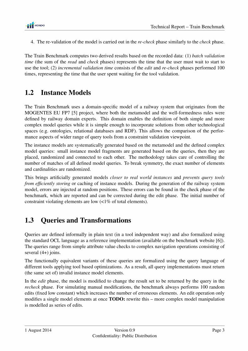
4. The re-validation of the model is carried out in the re-check phase similarly to the check phase.
The Train Benchmark computes two derived results based on the recorded data: (1) batch validationtime (the sum of the read and check phases) represents the time that the user must wait to start touse the tool; (2) incremental validation time consists of the edit and re-check phases performed 100times, representing the time that the user spent waiting for the tool validation.
1.2 Instance Models
The Train Benchmark uses a domain-specific model of a railway system that originates from theMOGENTES EU FP7 [5] project, where both the metamodel and the well-formedness rules weredefined by railway domain experts. This domain enables the definition of both simple and morecomplex model queries while it is simple enough to incorporate solutions from other technologicalspaces (e.g. ontologies, relational databases and RDF). This allows the comparison of the perfor-mance aspects of wider range of query tools from a constraint validation viewpoint.
The instance models are systematically generated based on the metamodel and the defined complexmodel queries: small instance model fragments are generated based on the queries, then they areplaced, randomized and connected to each other. The methodology takes care of controlling thenumber of matches of all defined model queries. To break symmetry, the exact number of elementsand cardinalities are randomized.
This brings artificially generated models closer to real world instances and prevents query toolsfrom efficiently storing or caching of instance models. During the generation of the railway systemmodel, errors are injected at random positions. These errors can be found in the check phase of thebenchmark, which are reported and can be corrected during the edit phase. The initial number ofconstraint violating elements are low (<1% of total elements).
1.3 Queries and Transformations
Queries are defined informally in plain text (in a tool independent way) and also formalized usingthe standard OCL language as a reference implementation (available on the benchmark website [6]).The queries range from simple attribute value checks to complex navigation operations consisting ofseveral (4+) joins.
The functionally equivalent variants of these queries are formalized using the query language ofdifferent tools applying tool based optimizations. As a result, all query implementations must return(the same set of) invalid instance model elements.
In the edit phase, the model is modified to change the result set to be returned by the query in therecheck phase. For simulating manual modifications, the benchmark always performs 100 randomedits (fixed low constant) which increases the number of erroneous elements. An edit operation onlymodifies a single model elements at once TODO: rewrite this – more complex model manipulationis modelled as series of edits.
1 August 2014 Version 0.9Confidentiality: Public Distribution
Page 3

Technical Report – Train Benchmark
1.4 Evaluation of Measurements
The Train Benchmark defines a Java-based framework and application programming interface thatenables the integration of additional metamodels, instance models, query implementations and evennew benchmark scenarios (which may be different from the original four-phase concept). The defaultimplementation contains a benchmark suite for queries implemented in Java, Eclipse OCL and EMF-INCQUERY.
Measurements are recorded automatically in a machine-processable format (CSV) that is automati-cally processed by R [7] scripts. An extended version of the Train Benchmark [23] features several(instance model, query-specific and combined) metrics that can be used to characterize the “diffi-culty” of benchmark cases numerically, and – since they can be evaluated automatically for otherdomain/model/query combinations – allow to compare the benchmark cases with other real-worldworkloads.
Page 4 Version 0.9Confidentiality: Public Distribution
1 August 2014

Chapter 2
Train Benchmark TechnicalSpecification
This chapter discusses the technical specification of the Train Benchmark. In order to ensure faircomparison of different tools, the specification describes the queries, transformations and the instancemodel generator in detail. The phases in the benchmark are also strictly defined.
Currently, the Train Benchmark comes in two versions: the original version (Section 2.1) and anextended version (Section 2.2), first discussed in paper [23].
2.1 Original Version
A test case configuration for every tool consists of an instance model (Section 2.1.6) with an instancemodel size, a predefined query (Section 2.1.4) describing constraint violating elements and the nameof the scenario (Section 2.1.2) to run.
As a result of a testcase run, the execution times of each phase, the memory usage and the number oferroneous elements are measured and recorded. The number of invalid elements are used to checkthe correctness of the validation, however the set of element identifiers must also be available forlater processing.
2.1.1 Phases
To measure performance for re-validating a model after modifications, four benchmark phases weredefined, as illustrated in Figure 2.1.
1. During the read phase, the previously generated instance model and validation query are loadedfrom hard drive to memory. This includes the parsing of the input as well as initializing datastructures of the tool.
5

Technical Report – Train Benchmark
Read Check
Metamodel
Instance model
Query specification
Edit Recheck!
Batch validation Incremental validation
Figure 2.1: The phases of the benchmark.
2. In the check phase, the instance model is queried to identify invalid elements. This can be assimple as reading the results from cache, or the model can be traversed based on some index.By the end of this phase, erroneous objects need to made available in a collection for furtherprocessing.
3. In the edit phase, the model is changed to simulate effects (and measure performance) of modelmodifying operations. At the beginning of this phase “query-like” functions are used to gatherelements to be modified, however this time is excluded, and only the required time of modelediting operations are recorded in this phase. (As query performance is measured in the checkphases.)
4. The re-validation of the model is carried out in the re-check phase similarly to the check phase.
2.1.2 Use Case Scenarios of the Benchmark
Paper [10] analyzes performance of algorithms used for graph pattern query evaluation and identi-fies two use cases where efficient incremental model validation is required. The batch part of ourbenchmark consists of the execution of the read and first check phases. Inspired by paper [10], threescenarios were defined to measure different use cases:
• Batch validation scenario (Batch): In this scenario the model is read in one batch from storage,than a model validation is carried out by executing the query in the check phase. Such use caseis performed when a model editor is opened and initial validations are issued by the designer.• Model transformation scenario (XForm): The automated model transformation scenario ex-
tends the batch validation scenario by differential model modification and re-checking phases.In the edit phase, the model is corrected, based on the erroneous objects identified during thebatch validation. This is carried out by the tool itself performing mass edits automatically.Finally, the whole model is re-checked, and remaining or newly introduced errors are reported.Efficient execution of such a use case is necessary during refactoring, incremental code gener-ation, or when a model is transformed from a source language to a target language by a modeltransformation program, using model synchronisation.• User model editing scenario (User): The user model editing scenario extends the batch val-
idation scenario by differential model modification and re-checking phases. After the batchvalidation a small model manipulation step is performed (e.g. a reference is deleted), which
Page 6 Version 0.9Confidentiality: Public Distribution
1 August 2014

Technical Report – Train Benchmark
is immediately followed by re-validation to get instantaneous feedback. In this scenario suchsmall edit and re-check phases are executed in sequence.Such scenario occurs when someone uses a common UML editor (for designing software so-lutions), or a domain-specific editor where elements or relations are added one-by-one. Theseeditors should detect design errors quickly and early in the development process to let engi-neers refine models and cut down debugging and error correction costs.
2.1.3 Metamodel
Route
Segment
length : EInt
SensorSignal
actualState : SignalStateKind
Switch
actualState : SwitchStateKind
SwitchPosition
switchState : SwitchStateKindTrackElement
SwitchStateKind
FAILURE
LEFT
RIGHT
STRAIGHT
SignalStateKind
STOP
FAILURE
GO
1 + route
* + switchPosition
2..*+ routeDefinition
1 + exit
1 + entry
*+ sensor
*+ trackElement
*
+ connectsTo
* + switchPosition
1 + switch
Figure 2.2: The railway metamodel used in the Train Benchmark.
The metamodel of the railway domain used in the Train Benchmark is depicted in Figure 2.2. A trainroute can be defined by a set of sensors. Sensors are associated with track elements: track segments(with a specific length) or a switches. A route may have associated switch positions which describethe required state of a switch belonging to the route. Different route definitions can specify differentstates for a specific switch.
2.1.4 Queries
In the validation and re-validation phases of the benchmark, the queries return the elements violatingthe well-formedness constraint defined by the test case. These constraints are first defined informallyin plain text and then formalized using a query language suited for the benchmarked tool. As a result,the query must return a set of the invalid instance model elements’ identifiers.
Two simple queries involving maximum 2 objects (PosLength and SwitchSensor) and two complexqueries involving 4–8 objects and multiple join operations (RouteSensor and SignalNeighbor) weredefined. Simple queries are able to quickly distinguish efficient tools from inefficient ones, whilecomplex queries are used to differentiate faster model query technologies.
1 August 2014 Version 0.9Confidentiality: Public Distribution
Page 7

Technical Report – Train Benchmark
In the following, we present the queries defined in the Train Benchmark. We describe the semanticsand the goal of each query. We also show the associated graph pattern and relational algebra query.
Relational Schemas
For formulating the queries in relational algebra we define the following relational schemas for rep-resenting the vertices (objects) in the graph (instance model).
• Route (id)• Sensor (id, Segment_length)• Signal (id)• Switch (id)• SwitchPosition (id)• TrackElement (id)
The edges (relationships) are represented with the following relational schemas:
• entry (Route, Signal)• exit (Route, Signal)• switchPosition (Route, SwitchPosition)• routeDefinition (Route, Sensor)• switch (SwitchPosition, Switch)• sensor (Switch, Sensor)• connectsTo (TrackElement, TrackElement)
Graph Patterns
In the following, we represent the graph pattern representation for the violation of each well-formedness constraint. Opaque blue rectangles and dashed arrows mark positive constraints, whilered rectangles and arrows represent negative application conditions (NACs). The result of the query(also referred as the match set) is marked with transparent blue rectangles. Additional constraints(e.g. arithmetic comparisons) are shown in the figure in text.
PosLength
Description. The PosLength well-formedness constraint requires that a segment must have positivelength. Therefore, the query (Figure 2.4) checks for segments with a length less than or equal to zero.The SPARQL representation of the query is shown in Figure 2.3.
Goal. The query checks whether an object has an attribute. If it does, the value is checked. Check-ing attributes is a real world use case, even if a very simple one. Note that simple string checking isalso measured in the Berlin SPARQL Benchmark [14] and it concludes that for most tools the stringcomparison algorithm dominates the query time.
Page 8 Version 0.9Confidentiality: Public Distribution
1 August 2014

Technical Report – Train Benchmark
1 SELECT DISTINCT ?xSegment WHERE {2 ?xSegment rdf:type base:Segment .3 ?xSegment base:length ?xLength .45 FILTER (?xLength <= 0)6 }
Figure 2.3: PosLength query in SPARQL.
segment: Segment
segment.length 0
Figure 2.4: The PosLength pattern.
Relational algebraic form. The PosLength query can be formalized in relational algebra as:
πid(σlength≤0 (Sensor)
)RouteSensor
Description. The RouteSensor well-formedness constraint requires that all sensors that are asso-ciated with a switch that belongs to a route must also be associated directly with the same route.Therefore, the query (Figure 2.7) looks for sensors that are connected to a switch, but the sensor andthe switch are not connected to the same route. The SPARQL representation of the query is shownin Figure 2.5.
Goal. This pattern checks for the absence of circles, so the efficiency of the join and the antijoinoperations is tested.
1 SELECT DISTINCT ?xSensor WHERE {2 ?xRoute rdf:type base:Route .3 ?xSwitchPosition rdf:type base:SwitchPosition .4 ?xSwitch rdf:type base:Switch .5 ?xSensor rdf:type base:Sensor .6 ?xRoute base:switchPosition ?xSwitchPosition .7 ?xSwitchPosition base:switch ?xSwitch .8 xSwitch base:sensor ?xSensor .910 FILTER NOT EXISTS {11 ?xRoute ?routeDefinition ?xSensor .12 } .13 }
Figure 2.5: The RouteSensor query in SPARQL 1.1.
Remark. Note that the negative application condition (NAC) part (FILTER NOT EXISTS) is aSPARQL 1.1 feature. In SPARQL 1.0, we have to use the approach shown in Figure 2.6.
1 August 2014 Version 0.9Confidentiality: Public Distribution
Page 9

Technical Report – Train Benchmark
1 OPTIONAL {2 ?xRoute ?routeDefinition ?xSensor .3 FILTER (sameTerm(base:routeDefinition,4 ?routeDefinition))5 } .6 FILTER (!bound(?routeDefinition))
Figure 2.6: The NAC of the RouteSensor pattern inSPARQL 1.0.
sensorrouteDefinition switch
switchPosition
switch: Switch
sp: SwitchPositionroute: Route
sensor: Sensor
Figure 2.7: The RouteSensor pattern.
Relational algebraic form. The RouteSensor query can be formalized in relational algebra as:
πRoute(switchPosition ./ switch ./ sensor . routeDefinition
)
SignalNeighbor
Description. The SignalNeighbor well-formedness constraint requires that the routes that are con-nected through sensors and track elements have to belong to the same signal. Therefore, the query(Figure 2.9) checks for routes which have an exit signal and a sensor connected to another sensor(which is in a definition of another route) by two track elements, but there is no other route that con-nects the same signal and the other sensor. The SPARQL representation of the query is shown inFigure 2.8.
Goal. This pattern checks for the absence of circles, so the efficiency of the join operation is tested.One-way navigable references are also present in the constraint, so the efficient evaluation of theseare also tested. Subsumption inference is required, as the two track elements can be switches orsegments.
Relational algebraic form. The SignalNeighbor query can be formalized in relational algebra as:
Page 10 Version 0.9Confidentiality: Public Distribution
1 August 2014

Technical Report – Train Benchmark
1 SELECT DISTINCT ?xRoute1 WHERE {2 ?xRoute1 rdf:type base:Route .3 ?xSen1 rdf:type base:Sensor .4 ?xRoute1 base:routeDefinition ?xSen1 .5 ?xTE1 rdf:type base:TrackElement .6 ?xTE1 base:sensor ?xSen1 .7 ?xTE2 rdf:type base:TrackElement .8 ?xTE1 base:connectsTo ?xTE2 .9 ?xSen2 rdf:type base:Sensor .10 ?xTE2 base:sensor ?xSen2 .11 ?xSig rdf:type base:Signal .12 ?xRoute1 base:exit ?xSig .1314 ?xRoute3 rdf:type base:Route .15 ?xRoute3 base:routeDefinition ?xSen2 .16 FILTER ( ?xRoute3 != ?xRoute1 )1718 OPTIONAL {19 ?xRoute2 rdf:type base:Route .20 ?xRoute2 base:routeDefinition ?xSen2 .21 ?xRoute2 base:entry ?xSig .22 } .23 FILTER (!bound(?xRoute2))24 }
Figure 2.8: The SignalNeighbor query in SPARQL.
πentry.Route(σentry.Route6=routeDefinition2.Route
(entry ./ routeDefinition1 ./ sensor1 ./
connectsTo ./ sensor2 ./ routeDefinition2 .(exit ./ routeDefinition3
)))SwitchSensor
Description. The SwitchSensor well-formedness constraint requires that every switch must haveat least one sensor connected to it. Therefore, the query (Figure 2.11) checks for switches that haveno sensors associated with them. The SPARQL representation of the query is shown in Figure 2.10.
Goal. This query checks whether an object is connected to a relation. This pattern is common inmore complex queries, e.g. it is used in the RouteSensor and the SignalNeighbor queries.
Relational algebraic form. The SwitchSensor query can be formalized in relational algebra as:
Switch . Sensor
1 August 2014 Version 0.9Confidentiality: Public Distribution
Page 11

Technical Report – Train Benchmark
connectsTo
routeDefinition
exit
sensor sensor
routeDefinition
routeDefinition
entry
route1 != route3
te1: TrackElement
sensor1: Sensor
route1: Route
signal: Signal
te2: TrackElement
sensor2: Sensor
route3: Route
route2: Route
Figure 2.9: The SignalNeighbor pattern.
1 SELECT DISTINCT ?xSwitch WHERE {2 ?xSwitch rdf:type base:Switch .34 FILTER NOT EXISTS {5 ?xSensor rdf:type base:Sensor .6 ?xSwitch base:sensor ?xSensor .7 } .8 }
Figure 2.10: The SwitchSensor query in SPARQL.
2.1.5 Transformations
In the edit phase the model is modified to change the result set returned in the succeeding re-checkphase.
The Train Benchmark defines a quick fix model transformation for each query. The transformationsare also represented as graph transformations. The insertions are shown in green with a «new»caption, while deletions are marked with a red cross and a «del» caption. In general, the goal of thesetransformations is to remove a subset of the invalid elements from the model.
Table 2.1. shows the instance model characteristics and the effect of the modify phase in the Route-Sensor case. The first column counts the number of instance model elements. The second and thefifth column show the number of Sensors in the model. The two scenarios process different instancemodels and modify them differently:
• In the User scenario (where a developer is assumed to sit in front of an editor) the initialnumber of constraint violating elements are low (0.3% of model elements for the RouteSensorcase), so it can be understood and resolved by a user using the editor.
Page 12 Version 0.9Confidentiality: Public Distribution
1 August 2014

Technical Report – Train Benchmark
sensor
switch: Switch
sensor: Sensor
Figure 2.11: The SwitchSensor pattern.
User (modify = 10) Model transformation (modify = Res1 × 10%)#Objects #Sensors Result1 Modify RS Result2 #Sensors Result1 Modify RS Result2
6032 928 19 10 29 967 94 9 8511710 1804 41 10 51 1936 193 19 17423180 3575 68 10 76 3545 348 34 31446728 7210 140 10 150 6691 642 64 57887396 13465 264 10 274 13650 1301 130 1171
175754 27074 510 10 520 27190 2606 260 2346354762 54653 1048 10 1058 55708 5324 532 4792708770 109185 2071 10 2081 110291 10623 1062 9561
1415954 218140 4215 10 4224 219305 21097 2109 189882837336 437089 8501 10 8510 437025 41762 4176 37586
Table 2.1: Modification in the RouteSensor test case.
During the modification the user always performs 10 random edits (fixed low constant) whichincrease the number of erroneous elements. These edit operations modify only some elementsof the model and do not add or remove modules containing multiple instance model elements.• In the model transformation scenario the initial number of errors is higher (1.5% of objects for
the RouteSensor case). This scenario models the case when these errors are processed by amodel transformation program automatically.In the edit phase the program modifies 10% of the elements of the result set retrieved fromthe batch query. These modifications always correct an invalid element in the model, so thenumber of invalid elements decreases (see Table 2.2).
Table 2.2. displays the effect of model changes to the result set size and the type of edit operations(add, update, delete).
User Model transformationModification type RSS change Modification type RSS change
PosLength Update Increase Update DecreaseSwitchSensor Delete Increase Add DecreaseRouteSensor Delete Increase Delete DecreaseSignalNeighbor Update Increase Update Decrease
Table 2.2: Modification type for the queries.
The modifications in more detail:
• User scenario: in this case elements to be edited are selected from the whole instance model,i.e. they may be valid or invalid.
1 August 2014 Version 0.9Confidentiality: Public Distribution
Page 13

Technical Report – Train Benchmark
length = length + 1
segment.length 0
segment: Segment
Figure 2.12: The PosLength transformation in the Model transformation scenario.
sensorrouteDefinition switch
switchPosition
switch: Switch
sp: SwitchPositionroute: Route
sensor: Sensor«del»
Figure 2.13: The RouteSensor transformation in the Model transformation scenario.
• PosLength: Randomly selected segments’ length attribute is updated to 0, which meansthat an error is injected (Figure 2.16a).In EMF this means that an int attribute is set (updated), while in other representations(e.g. RDF databases) first the assertion about the old value is removed and the assertionstating the new value of the length is inserted.• RouteSensor: The routeDefinition edges between the randomly selected routes and their
first connected sensor are removed (Figure 2.16b).• SignalNeighbor: Errors are introduced by disconnecting the entry edge of the selected
routes (Figure 2.16c).• SwitchSensor: Errors are injected by randomly selecting switches and deleting their rela-
tionship to sensors. If the chosen switch was invalid, it did not have such a relationship,so no relationships are deleted and the switch stays invalid. If the chosen switch was valid,it will become invalid (Figure 2.16d).
• Model transformation scenario: in this case elements to be edited are selected from the resultof the previous query. The transformations provide quick fix-like refactoring operations.
• PosLength: Random elements are selected from the set of invalid segments and theirvalues are updated to –oldValue + 1 (Figure 2.12).• RouteSensor: Randomly selected invalid sensors are disconnected from the switch, which
means that the constraint will no longer apply (Figure 2.13).• SignalNeighbor: Disconnect exit references of randomly selected invalid routes, resulting
in a structure where the constraint must not hold for the actual route (Figure 2.14).• SwitchSensor: Random elements are selected from the set of invalid switches and are
connected to newly created sensors.In EMF this means the creation of a new Sensor which is added to the switch and alsoto the root container object. In ontology the triples asserting the connection betweenthe new Sensor and the Switch, as well as its type are inserted into the knowledge base(Figure 2.15).
Page 14 Version 0.9Confidentiality: Public Distribution
1 August 2014

Technical Report – Train Benchmark
connectsTo
routeDefinition
exit
sensor sensor
routeDefinition
routeDefinition
entry
route1 != route3
te1: TrackElement
sensor1: Sensor
route1: Route
signal: Signal
te2: TrackElement
sensor2: Sensor
route3: Route
route2: Route
«del»
Figure 2.14: The SignalNeighbor transformation in the Model transformation scenario.
sensor
sensor: Sensor
sensor: Sensor
sensor«new»
«new»
switch: Switch
Figure 2.15: The SwitchSensor transformation in the Model transformation scenario.
2.1.6 Instance Model Generation
In the first phase of the benchmark, a previously generated instance model is loaded from the file sys-tem. These models are systematically generated based on the metamodel and on the model queries.Randomized instance model fragments are generated and connected to each other. The generationprocess takes care of controlling the number of matches for all model queries.
To break symmetry, the exact number of elements and cardinalities are randomized. This bringsartificially generated models closer to real world instances, and prevents query tools from this kindof efficient storing of instance models. During the generation of the railway system model, errorsare injected at random positions. The initial number of constraint violating elements that are low(below one percent of the total number of elements), and are deterministically placed, thanks topseudorandom generation. These errors have to be found in the check phase of the benchmark, andcan be corrected during the edit phase.
1 August 2014 Version 0.9Confidentiality: Public Distribution
Page 15

Technical Report – Train Benchmark
length 0
segment: Segment
(a) PosLength
routeDefinition
route: Route
sensor: Sensor
«del»
(b) RouteSensor
entry
route: Route
signal: Signal
«del»
(c) SignalNeighbor
sensor
switch: Switch
sensor: Sensor
«del»
(d) SwitchSensor
Figure 2.16: Transformations in the User scenario.
SignalactualState : SignalStateKind
Route Sensor TrackElement
SwitchactualState : SwitchState
Segment length : Int
SwitchPositionswitchState : SwitchState
entry
exit
trackElement
switchPosition
switch
connectsTo
sensor
switchPosition
route
routeDefinition
0.4%0.4%
3.4%
80.4%
3.4%
0.9
0.9
41
6
Sw: 4.4
11
9.5
1
1
15.4%
77.0%
Seg: 1
Figure 2.17: The railway metamodel and instance model characteristics.
To show some characteristics of the generated instance models, the distribution of the object typesand the average number of edges for each object are presented in Figure 2.2. In the case of classes thepercentage of instances is shown: e.g. 3.4% of the model elements are instance of the class Switch,77.0% are Segments, thus 80.4% are TrackElements. The average number of the given relation for aninstance is displayed for associations: e.g. there are 9.5 switchPosition relations in average for everyinstance of the Route class.
2.2 Extended version
Section 2.1 describes a benchmark that can be used to compare performance of different tools. ThisSections extends this benchmarking conecpt by characterizing instance models and queries by met-rics, and evaluate which tools are the most sensitive to which metrics.
Page 16 Version 0.9Confidentiality: Public Distribution
1 August 2014

Technical Report – Train Benchmark
2.2.1 Overview
The aim of our metrics and benchmarking scenarios is to give a precise mechanism for identifyingkey factors in selecting between different query evaluation technologies.
The presented metrics for our evaluation (see in Section 2.2.2) were constructed based on a set ofalready and widely used metrics, extended with two more specific ones that aims to give a grossupper bound on the cost of query evaluation.
For the benchmark scenario we opted for a simple execution schema that represents a batch validationscenario. This is the same as the first two phase of the original benchmark. See Figure 2.1 andSection 2.1.1 for a description of the read and check phases.
2.2.2 Metrics
Our investigation relies on a selection of metrics that quantitatively describe the task of a certainquery, independently of the actual strategy or technological solution that provides the query results.Broadly speaking, such a querying task consist of (a) an instance model, (b) a query specificationthat defines what results should be yielded, (c) a runtime context in which the queries are evaluated,such as the frequency of individual query evaluations and model manipulation inbetween.
The metrics discussed in the following, characterize instance models, queries or their combination,without characterizing a unique property of a specific graph/query description language or environ-ment. Most of these metrics have previously been defined by other sources, while others are newlyproposed in this paper.
Metrics for Instance Model Only
Clearly, properties of the instance model may have a direct effect on query performance, e.g. queryinglarger models may consume more resources.
A first model metric is model size, which can be defined either as the number of objects (metriccountNodes), the number of references (edges) between objects (countEdges), the number ofattribute value assignments (not used in the paper); or some combination of these three, such as theirsum (countTriples), which is basically the total number of model elements / RDF triples. This iscomplemented by the number of different classes the objects in the model belong to (countTypes),and the instance count distribution of the classes. Additional important model metrics characterizethe distribution of the out-degrees and in-degrees (the number of edges incident on an object), partic-ularly the maximum and average degrees (maxInDegree, maxOutDegree, avgInDegree andavgOutDegree).
The metrics discussed above have been defined e.g. in [28], along with other metrics such as therelative frequencies of the edge label sequences of directed paths of length 2 or 3.
1 August 2014 Version 0.9Confidentiality: Public Distribution
Page 17

Technical Report – Train Benchmark
Metrics for Query Specification Only
The query specification is a decisive factor of performance as well, as complex queries may be costlyto evaluate. Such query metrics can be defined separately, in several query formalisms. Due tothe close analogies between graph patterns and SPARQL queries, we can consider these metricsapplying to graph pattern-like queries in general. This allows us to formulate and calculate metricsexpressed on the graph patterns interpreted by EMF-INCQUERY, and characterize the complexity ofthe equivalent SPARQL query with the same metric value.
As superficial metrics for graph pattern complexity, we propose the number of variables(numVariables) and the number of parameter variables (numParameters); the number ofpattern edge constraints (numEdgeConstraints) and the number of attribute check constraints(numAttrChecks); finally the maximum depth of nesting NACs (nestedNacDepth). Someof these are similar/equivalent to SPARQL query metrics defined in [19]. Other metrics proposedby [19] are mostly aimed at measuring special properties relevant to certain implementation strate-gies.
Metrics for Combination of Query and Instance Model
The following two metrics (defined previously in literature) characterize the query and the instancemodel together.
The most trivial such metric is the cardinality of the query results (metric countMatches); intu-itively, a query with a larger result set typically takes longer to evaluate on the same model, while asingle query is typically more expensive to evaluate on models where it has more matches. The met-ric selectivity is proposed by [19], is the ratio of the number of results to the number of modelelements (i.e. countMatches/countTriples).
New Metrics for Assessing Query Evaluation Difficulty
We propose two more metrics that take query and instance model characteristics into account. Ouraim is to provide a gross upper bound on the cost of query evaluation. We consider all enumerableconstraints in the query, for which it is possible to enumerate all tuples of variables satisfying it;thus edge constraints and pattern composition are enumerable, while NACs and attribute checks ingeneral are not. At any given state of evaluation, a hypothetical search-based query engine has eitheralready identified a single occurrence of an enumerable constraint c (e.g. a single instance of an edgetype for the corresponding edge constraint), or not; there are therefore |c| + 1 possible cases for c,where |c| is the number of different ways that c can be satisfied in the model. This gives
∏c 1 + |c|
as the overestimate of the search space of the query evaluator. To make this astronomical figuremanageable, we propose the absolute difficulty metric (absDifficulty) as the logarithm of thesearch space size, i.e. ln
∏c (1 + |c|) =
∑c ln(1 + |c|).
The result size is a lower bound of query evaluation cost, since query evaluation takes at least asmuch time or memory as the number of results. It is therefore expected that queries with a highnumber of matches also score high on the absolute difficulty metric. To compensate for this, the
Page 18 Version 0.9Confidentiality: Public Distribution
1 August 2014

Technical Report – Train Benchmark
relative difficulty metric (relDifficulty) is defined as ln∏
c (1+|c|)1+countMatches =
∑c ln(1 + |c|) – ln(1 +
countMatches), expressing the logarithm of the “challenge” the query poses – this is how muchworse a query engine can do than the lower bound. If the relative metric is a low figure, than thecost of query evaluation will not be much worse than the optimum, regardless of the query evaluationstrategy. It can be easily shown that if a part of a graph pattern is extracted as a helper pattern thatis used via pattern composition, then the sum of the relative difficulties of the two resulting patternswill be the same as the relative difficulty of the original pattern. This suggests that this metric shouldbe treated as additive over dependent queries, and also that it is worth extracting common parts ofmultiple patterns into reusable helper patterns.
2.2.3 Modified Metamodel
Route
Segment
length : EInt
height : EInt
Sensor
year : EInt
Signal
Switch
state
SwitchPosition
state
TrackElement
+ route
+ switchPosition
+ routeDefinition
1 + exit
1 + entry
+ sensor
+ trackElement
+ connectsTo
+ switchPosition
+ switch
Figure 2.18: The railway metamodel (metrics version).
The metamodel used for merics evaluation is depicted in Figure 2.18. This is similar to the onepresented in Section 2.1.3, but cardinality constraints are mostly omitted, and height and year integerattributes are introduced for classes Segment and Sensor respectively. This gives higher freedom forthe instance model generator, and more queries can be defined for attribute checks.
2.2.4 Instance Models for the Modified Metamodel
Models are characterized by their size and structure. Here size refers to the cardinalities of node andedge types. The fact that increasing model size tends to increase the cost of queries is intuitivelyself evident (and also empirically confirmed e.g. by our previous experiments [10, 11]). Handlinglarge models in real life is a great chellenge, but model structure (that determines which nodes areconnected to each other by which edges) must also be taken into account, which here means edge
1 August 2014 Version 0.9Confidentiality: Public Distribution
Page 19

Technical Report – Train Benchmark
distribution of nodes. Different edge distributions also present in real-world networks: the inter-net or protein-protein interaction networks show scale-free characteristics [9], while in other areasself-healing algorithms for binomial computer networks are studied [8]. Average degree can impactperformance greatly, which is a typical property of different model kinds. For example, softwaremodels have usually nodes with low degree, while social models are usually dense graphs.
We have conducted the experiments on synthetic models, generated automatically with our modelbuilder, belonging to three model families (without comparing them directly to real world ones, leav-ing it as a future work). All generated models within a family have the same approximate size; thoughthere is some random variation due to the generation process (see later), with low standard deviation(e.g. measured as 0.3% in family A). Family A models are relatively dense graphs (~26 edges/n-odes, i.e. metric avgOutDegree) with 1.8 million total model elements (metric numTriples);family B models are equally dense, but are scaled back to only 113 thousand elements; finally fam-ily C models have almost 1.3 million model elements that form a relatively sparse graph (8.4 – 8.7edges/nodes).
Each model of a family has the same (expected) number of instances for any given type. However,these models of the same size still differ in their internal structure. Given the cardinalities of eachtype, our generator first created the instance sets of node types, along with generating attribute valuesaccording to an associated distribution. Then for each edge type, the generator created edge instances(with the given expected cardinality) between instances of the source type and instances of the targettype. The structure of the graph is induced by the method of choosing which source node and whichtarget node to connect. We have applied the following four methods, each taking as input the set Sof source node candidates, the set T of target node candidates, and the expected cardinality e of theedge type.
Binomial case. Inspired by the well-known Erdos-Rényi model of random graphs [16], the firstapproach is to take each pair of source and target nodes, and draw an edge between them with a givenprobability p. This makes the expected cardinality of edges e = p × |S| × |T|, thus p is chosen as
e|S|×|T| . The degrees of nodes will be binomially distributed, e.g. out-degrees with parameters |T| andp.
Hypergeometric case. While the previous solution ended up with a random number of edges (withexpected value e), this slightly different approach will generate exactly e edges, by taking each pairof source and target nodes, and randomly selecting e from them into the graph. The degrees will behypergeometrically distributed, e.g. out-degrees with parameters |S|× |T|, |T| and e.
Regular case. In software engineering models, one often finds for a given edge type that out-degreesof all nodes of the source type are roughly equal, and the same is true for in-degrees. This motivateda method that tries to uniformly (but randomly) divide e edges between the source nodes, so that thedifference between any two out-degrees is at most 1; while also dividing the same edges between thetarget nodes, with a similar restriction on in-degrees.
Scale-free case. It has been observed in many different disciplines that degree distributions of certainlarge graphs follow a power law, especially growing / evolving graphs with the preferential attach-ment property (a new edge is more likely to connect to a node which already has a higher degree).We have used a variant of the preferential attachment bipartite graph generator algorithm of [32] togenerate the connections from source nodes to target nodes.
Page 20 Version 0.9Confidentiality: Public Distribution
1 August 2014

Technical Report – Train Benchmark
Model Family Model structure countNodes countEdges countTriples countTypes avgOutDegree avgInDegree maxOutDegree maxInDegreeA Regular 63289 1646386 1811752 7 26.01 26.01 63288 44A Binomial 63289 1649179 1814545 7 26.06 26.06 63288 69A HyperGeo 63289 1646386 1811752 7 26.01 26.01 63288 74A Scalefree 63289 1660033 1825399 7 26.23 26.23 63288 10390B Regular 3954 102839 113170 7 26.01 26.01 3953 44B Binomial 3954 102984 113315 7 26.05 26.05 3953 64B HyperGeo 3954 102839 113170 7 26.01 26.01 3953 69B Scalefree 3954 96029 106360 7 24.29 24.29 3953 918C Regular 120001 1040000 1280001 7 8.67 8.67 120000 13C Binomial 120001 1041323 1281324 7 8.68 8.68 120000 30C HyperGeo 120001 1040000 1280001 7 8.67 8.67 120000 29C Scalefree 120001 1012858 1252859 7 8.44 8.44 120000 8929
Table 2.3: Values of model metrics on the generated instance models.
The four generation methods induced significantly different degree distributions. This and otherdifferences are shown in Table 2.3.
One-to-many relationships were treated in a special way to meet the multiplicity restriction. In par-ticular, a single top-level container element (not depicted in the metamodel figure, neither involvedin any queries) was used to contain all elements; it therefore has an outgoing containment edge forevery other object, thereby “polluting” the maxOutDegree metric.
2.2.5 Benchmark Queries
Based on the previously defined metrics for query specification and based on the metamodel, sixseries of model query specifications were systematically constructed. Each query series includesfour to seven model queries that aim to be different in only one of the defined model query metrics.Executing a query series on the same model and tool results in a data series that shows how the toolis scalable according to the represented model metric.
Locals Query Series for the numVariables Metric
Five queries were defined, where each one includes the same number of edge constraints, but thenumber of local variables increases.
It can be realized using the Segment type and connectsTo reference, so it means that only onenode type and reference type is used in these patterns and the focus is on the structure of the patterns.The simple graph based visualisation of these pattern structures is shown in Figure 2.19, where thenode drawn with empty circle represents the single pattern parameter.
3
22
3 4
2 3
4 5
2
3
45
6
2 3
4
5
7
6
Figure 2.19: The Locals patterns.
1 August 2014 Version 0.9Confidentiality: Public Distribution
Page 21

Technical Report – Train Benchmark
Refs Query Series for the numEdgeConstraints Metric
The Refs query series is also constructed based on the Segment type and connectsTo reference.
Here, the number of edge constraints increases along the series, but the number of local variables isconstant in all of the generated four queries. The visualisation of these pattern structures is shown inFigure 2.20.
Figure 2.20: The Refs patterns.
Params and ParamCircle Query Series for the numParameters Metric
Two series of queries were constructed for this metric, because of performance reasons. The Paramsquery series is the more complex and some tools exceed the time limit in the benchmark. TheParamsCircle query series is a simplification of the Params series.
The goal of this constructed query series is to create patterns with the same body, but with an in-creasing number of parameters. The first of these queries (returning one parameter) is shown inFigure 2.21, where the parameter is the blue object. Other queries use the same body, but add sen1,then sen2, then other variables to the parameter list.
routeDefinition
trackElement trackElement
seg1: Segment
sen1: Sensor
r: Route
sw: Switch
sen2: Sensor
routeDefinition
swP: SwitchPosition
switchPosition
route
trackElement
r: Route
sw: Switch
sen2: Sensor
routeDefinition
swP: SwitchPosition
switchPosition
route
Figure 2.21: The Params and ParamsCircle pattern schemas (first step).
Checks Query Series for the numAttrChecks Metric
Each Checks query use the same pattern body described by the pattern schema in Figure 2.22,but each one is extended with an increasing number of attribute check constraints. These checkconstraints filter results based on the year, height and length value of the segments seg1 and seg2,resulting in seven queries.
Page 22 Version 0.9Confidentiality: Public Distribution
1 August 2014

Technical Report – Train Benchmark
routeDefinition
trackElement trackElement
check(seg1.length < 10)
seg1: Segment
sen1: Sensor
r: Route
seg2: Segment
sen2: Sensor
routeDefinition
Figure 2.22: The Checks pattern schema.
Negs Query Series for the nestedNacDepth Metric
Negs queries present increasing number of nested neg constraints. These queries are defined basedon the following schema: at the bottom there is a pattern checking for segments with length lessthan ten. Next, for each query a new segment is matched, and the previous pattern is encapsulatedin a negative pattern call. i = 5 queries are defined in the benchmark, described by the schema inFigure 2.23.
connectsTo
Seg(i 1): Segment
connectsTo
Seg(i 2): Segment
Seg(i): Segment
connectsTo
connectsToSeg(i 3): Segment
...
connectsTo
Figure 2.23: The Negs pattern schema.
After the construction of the query series, we evaluated the query only metrics on them. Table 2.4shows the results of the evaluation: each cell contains the value or range of values that we got oneach query series. This table confirms that there are query series for every metric (shown in blue),and each query series differ in one or more metrics.
1 August 2014 Version 0.9Confidentiality: Public Distribution
Page 23

Technical Report – Train Benchmark
Query series numParameters numVariables numEdgeConstraints numAttrChecks nestedNacDepthParam 1–5 8 8 0 0ParamCircle 1–5 6 6 0 0Locals 1 3–7 6 0 0Refs 1 5 4–7 0 0Checks 1 5–11 4–10 0–6 0Neg 2–6 3–11 1–5 1 0–10
Table 2.4: Query-only metrics.
2.2.6 Complex Analysis
2.3 Implementation architecture
In this chapter, we discuss the implementation details of the Train Benchmark. The installation guideis available in the MONDO wiki.1
For the integration of the Train Benchmark projects and their third party dependencies, we useApache Maven [1]. The dependencies are shown in Figure 2.24.
In this section, we briefly describe the tasks and responsibilities of each module. The modules aregrouped to Maven build profiles which can be built separately.
2.3.1 Parent module
The hu.bme.mit.trainbenchmark module is the parent module which contains the modulesused in the Train Benchmark. Building this Maven module builds all child modules as well.
2.3.2 Central modules
The hu.bme.mit.trainbenchmark.model module contains the reference metamodel repre-sented in EMF.
The hu.bme.mit.trainbenchmark.config module contains classes and constants used bythe generator and the benchmark projects.
2.3.3 Representation-specific modules
The hu.bme.mit.trainbenchmark.emf and hu.bme.mit.trainbenchmark.rdfmodules contain classes and constants used by the particular representations.
1https://opensourceprojects.eu/p/mondo/wiki/TrainBenchmark/
Page 24 Version 0.9Confidentiality: Public Distribution
1 August 2014

Technical Report – Train Benchmark
benchmark.java
generator
benchmark.neo4j
generator.graph
generator.sql
generator.emf
generator.rdf
benchmark.rdf
benchmark.sesame
benchmark.drools
generator
Eclipse plug-in project Maven project Eclipse repositorylegend
benchmark
model emf config
benchmark.emf benchmark
benchmark.eclipseocl
benchmark.eclipseocl.
product
benchmark.emfincquery
benchmark.emfincquery.
patterns
benchmark.emfincquery.
product
benchmark.incqueryd
benchmark.fourstore
MANIFEST.MF dependency pom.xml dependency
benchmark.mysql
metrics
metrics
metrics.emf.iqpl
metrics.emf.iqpl.product
metrics.emf.iqpl.
querymetrics
metrics.rdf.sparql
model.ase
benchmark.emfincquery.
patterns.ase
generator.ase.incquery
generator.ase
rdf
Figure 2.24: The Maven modules defined in the Train Benchmark. Note that artifact ids of themodules are shortened and the full ids start with hu.bme.mit.trainbenchmark.
1 August 2014 Version 0.9Confidentiality: Public Distribution
Page 25

Technical Report – Train Benchmark
2.3.4 Generator modules
The hu.bme.mit.trainbenchmark.generator.* modules are responsible for generatingthe instance models for the benchmarks.
• emf: generates an EMF instance model.• emfuuid: generates an EMF instance model with UUIDs. A UUID (universally unique iden-
tifier) identifies an EObject uniquely, and is generated automatically by the EMF framework. Inthe output file, UUIDs are used to reference other objects, and not XPath expressions, speedingup the serialization process.• graph: generates a property graph model in the specified format: GraphML (default),
Blueprints GraphSON, Faunus GraphSON.• rdf: generates an RDF instance model.• sql: generates an SQL script which creates and loads the appropriate database tables.
2.3.5 Benchmark modules
The hu.bme.mit.trainbenchmark.benchmark.*modules are responsible for benchmark-ing. For the list of current implementations, see Table 3.1.
2.3.6 4store
To access 4store through a graph-like API, we developed a Java client with a focus on high perfor-mance.
• Homepage: https://git.inf.mit.bme.hu/w?p=projects/bigmodel/4store-graph-client.git• Clone URI: https://[email protected]/r/projects/bigmodel/4store-graph-client.git
Page 26 Version 0.9Confidentiality: Public Distribution
1 August 2014

Chapter 3
Benchmark Results
3.1 Benchmarking Environment
For the implementation details, source codes and raw results, see the benchmark website1. In thissection we describe the runtime environment, and highlight some design decisions.
The benchmark machine contains two dual-core Intel Xeon (3.00 GHz) CPU, 12 GBs of RAM andan SAS disk formatted to ext4 for storing the models. In order to alleviate disturbance of a runningmeasurement and minimize noise in the results, a bare metal 64-bit Ubuntu 12.10 OS was installedwith unnecessary services (like cron) turned off. Oracle JVM version 1.7.0_51 is used as the Javaenvironment and Eclipse Kepler Modeling 64-bit for Linux to satisfy specific tool dependencies.
The performance measurements of a tool was independent from the others, i.e. for every tool only itscodebase was loaded, and every measurement of a scenario was started in a different JVM. Before theexecution, the OS file cache was cleared, and swapping was disabled to avoid this kind of thrashing.Each test case (including all phases) must be run within a specified time limit (15 minutes), otherwiseits process was killed.
In the benchmark all cases were run 10 times, and the results were dumped into files, which wereaggregated using the R statistical framework. The correlation results and performance plots arewritten into an HTML report.
3.2 Tools
The measured tools generally work on graph-based models (like EMF [29] or RDF [33]), and providea graph pattern-like query language. Table 3.1 shows the list of currently integrated tools.
Note on incrementality: incremental means that the tool not only employs caching techniques, butprovides a dedicated incremental query evaluation algorithm that processes changes in the model andpropagates these changes to query evaluation results in an incremental way (i.e. avoiding complete
1https://incquery.net/publications/trainbenchmark/full-results
27
Technical Report – Train Benchmark
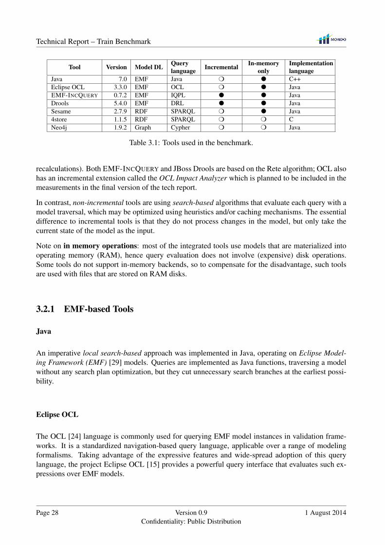
Tool Version Model DL Querylanguage Incremental In-memory
onlyImplementationlanguage
Java 7.0 EMF Java m l C++Eclipse OCL 3.3.0 EMF OCL m l JavaEMF-INCQUERY 0.7.2 EMF IQPL l l JavaDrools 5.4.0 EMF DRL l l JavaSesame 2.7.9 RDF SPARQL m l Java4store 1.1.5 RDF SPARQL m m CNeo4j 1.9.2 Graph Cypher m m Java
Table 3.1: Tools used in the benchmark.
recalculations). Both EMF-INCQUERY and JBoss Drools are based on the Rete algorithm; OCL alsohas an incremental extension called the OCL Impact Analyzer which is planned to be included in themeasurements in the final version of the tech report.
In contrast, non-incremental tools are using search-based algorithms that evaluate each query with amodel traversal, which may be optimized using heuristics and/or caching mechanisms. The essentialdifference to incremental tools is that they do not process changes in the model, but only take thecurrent state of the model as the input.
Note on in memory operations: most of the integrated tools use models that are materialized intooperating memory (RAM), hence query evaluation does not involve (expensive) disk operations.Some tools do not support in-memory backends, so to compensate for the disadvantage, such toolsare used with files that are stored on RAM disks.
3.2.1 EMF-based Tools
Java
An imperative local search-based approach was implemented in Java, operating on Eclipse Model-ing Framework (EMF) [29] models. Queries are implemented as Java functions, traversing a modelwithout any search plan optimization, but they cut unnecessary search branches at the earliest possi-bility.
Eclipse OCL
The OCL [24] language is commonly used for querying EMF model instances in validation frame-works. It is a standardized navigation-based query language, applicable over a range of modelingformalisms. Taking advantage of the expressive features and wide-spread adoption of this querylanguage, the project Eclipse OCL [15] provides a powerful query interface that evaluates such ex-pressions over EMF models.
Page 28 Version 0.9Confidentiality: Public Distribution
1 August 2014

Technical Report – Train Benchmark
EMF-INCQUERY
EMF-INCQUERY [11] is an Eclipse Modeling project that provides incremental query evaluationusing Rete [17] nets. Queries can be written in its graph pattern based query language (IncQueryPattern Language, IQPL [12]), which is evaluated over EMF models.
Drools
Incremental query evaluation is also supported by the Drools [4] rule engine developed by Red Hat.It is based on a variant of Rete [17] (object-oriented Rete). Queries can be formalized using itsown rule description language. Queries can be constructed by naming the ”when” part of rules andacquiring their matches. While Drools is not an EMF tool per se, the Drools implementation of theTrain Benchmark works on EMF models.
3.2.2 RDF-based Tools
Sesame
Sesame gives an API specification for many tools, and also provides its own implementation. Thetool evaluates queries over RDF that are formulated as SPARQL [34] graph patterns.
4store
4store [20] is an open source, distributed triplestore implemented in C. The main goal of 4store is toprovide a high performance storage and query engine for semantic web applications.
INCQUERY-D
INCQUERY-D [21] is a distributed incremental graph query engine developed in the Budapest Uni-versity of Technology and Economics. The goal of INCQUERY-D is to provide a scalable queryengine by using a cluster of servers instead of a single workstation.
3.2.3 Graph-based Tools
Neo4j
As part of the NoSQL movement, database management systems emerged with a focus on graphstorage and processing. As of 2014, the most popular graph database is Neo4j [3]. The data model isbased on graphs, where any node or edge can be labeled. Cypher can be used to query labeled graphsusing its own graph pattern notation. This engine also uses disk for data storing, so a RAM disk iscreated during the benchmark.
1 August 2014 Version 0.9Confidentiality: Public Distribution
Page 29

Technical Report – Train Benchmark
3.2.4 SQL-based Tools
MySQL
MySQL [2] is one of the most well-known and widely used open-source relational database manage-ment systems.
3.3 Measurement Results for Performance Comparison
The measurement results of the benchmark are displayed below. These diagrams show the batchquery performance and incremental evaluation time of each tool, for different model sizes. Addition-ally, the initial and the updated result set size is displayed under the model sizes for the batch andincremental queries, respectively.
3.3.1 How to read the charts
The charts are presented with logarithmic scales on both axes. This means that the general “lin-ear” appearance of all measurement series correspond to a low-order polynomial big-O characteristicwhere the slope of the plot determines the dominant order (exponent). Moreover, a constant differ-ence on these plots corresponds to a constant order-of-magnitude (i.e. constant multiplier) difference.As the execution runs with a timeout, incomplete measurement series indicate that the time limit hasbeen reached during execution.
The execution phases as described in Section 2.1.1 have been grouped into several aggregated resultsas follows:
• Batch validation (Section 3.3.2) corresponds to the sum of read and check execution times, asit models a batch validation scenario where the model is read and validated.• Revalidation (Section 3.3.3) corresponds to the sum of edit-recheck times as it represents the
cumulative execution time of model editing-revalidation cycles.• Total time (Section 3.3.4) represents the combined execution time of the entire measurement
cycle, giving an overall performance indicator.• Series of edit times (Section 3.3.5) presents a deeper analysis to show how long each edit-re-
check cycle takes. These plots are useful for observing transient effects such as JIT HotSpotcompilation.• Series of revalidation times (Section 3.3.6) present the same for the re-check phase.
Each plot shows execution times corresponding to a combination of one of the queries of Sec-tion 2.1.4 and a tranformation scenario as defined in Section 2.1.5. The plots offer insights intoperformance characteristics in three major ways:
• Execution time vs. instance model size. Each plot can be directly interpreted as an evalua-tion of performance against increasing model size, where different tool characteristics can becompared in a single plot.
Page 30 Version 0.9Confidentiality: Public Distribution
1 August 2014

Technical Report – Train Benchmark
• Characteristics vs. increasing query complexity. As the queries are of different complexity,comparing the plots within the same transformation scenario group but against different queriesis useful to judge tool characteristics against increasing query complexity (or query result size,shown as “Results” on the Y axis).• Characteristics vs. increasing transformation complexity. As the transformation scenarios
are characteristically different (e.g. with respect to the amount of objects modified by thetransformation sequence – as shown on the X axis as “Modifications”), comparing the plotswith the same query but against different scenarions is useful to judge tool characteristicsagainst various transformation complexities.
3.3.2 Batch Validation
Batch Validation (User Scenario)
●
●
●
●
●●
●
●
●●
●
●
●●
●
●
●
●
0.83
2.09
5.24
13.14
32.93
82.57
207.01
519.00
6k24k470
12k49k937
23k90k1769
43k170k3k
88k347k6k
176k691k13k
361k1M28k
715k2M55k
1M5M
110k
NodesEdgesResults
Tim
e [s
]
Tools
●
●
Eclipse OCLEMF−IncQueryJavaDroolsSesameNeo4jNeo4j RAM4store4store RAMMySQL
Batch validation time PosLength (x,y:logscale), User
Figure 3.1: Batch validation times for the PosLength query in the User scenario.
1 August 2014 Version 0.9Confidentiality: Public Distribution
Page 31

Technical Report – Train Benchmark
●
●
●
●
●
●
●
●
●●
●
●
●●
●
●
●
●
0.89
2.28
5.82
14.85
37.94
96.89
247.46
632.00
6k24k94
12k49k193
23k90k348
43k170k642
88k347k1301
176k691k2k
361k1M5k
715k2M10k
1M5M21k
NodesEdgesResults
Tim
e [s
]
Tools
●
●
Eclipse OCLEMF−IncQueryJavaDroolsSesameNeo4jNeo4j RAM4store4store RAMMySQL
Batch validation time RouteSensor (x,y:logscale), User
Figure 3.2: Batch validation times for the RouteSensor query in the User scenario.
●
●
●
●
●
●
●
●
●
0.91
2.18
5.20
12.41
29.63
70.72
168.82
403.00
6k24k2
12k49k3
23k90k5
43k170k11
88k347k14
176k691k31
361k1M59
715k2M115
1M5M225
NodesEdgesResults
Tim
e [s
]
Tools
●Eclipse OCLEMF−IncQueryJavaDroolsSesameNeo4jNeo4j RAM4store4store RAM
Batch validation time SignalNeighbor (x,y:logscale), User
Figure 3.3: Batch validation times for the SignalNeighbor query in the User scenario.
Page 32 Version 0.9Confidentiality: Public Distribution
1 August 2014

Technical Report – Train Benchmark
●
●
●
●
●●
●
●
●●
●
●
●●
●
●
●
●
0.83
2.09
5.25
13.14
32.93
82.51
206.73
518.00
6k24k19
12k49k46
23k90k91
43k170k162
88k347k326
176k691k637
361k1M
1287
715k2M2k
1M5M5k
NodesEdgesResults
Tim
e [s
]
Tools
●
●
Eclipse OCLEMF−IncQueryJavaDroolsSesameNeo4jNeo4j RAM4store4store RAMMySQL
Batch validation time SwitchSensor (x,y:logscale), User
Figure 3.4: Batch validation times for the SwitchSensor query in the User scenario.
Batch Validation (XForm Scenario)
●
●
●
●
●●
●
●
●●
●
●
●●
●
●
●
●
0.97
2.37
5.83
14.30
35.10
86.16
211.46
519.00
6k24k470
12k49k937
23k90k1769
43k170k3k
88k347k6k
176k691k13k
361k1M28k
715k2M55k
1M5M
110k
2M11M221k
NodesEdgesResults
Tim
e [s
]
Tools
●
●
Eclipse OCLEMF−IncQueryJavaDroolsSesameNeo4jNeo4j RAM4store4store RAMMySQL
Batch validation time PosLength (x,y:logscale), XForm
Figure 3.5: Batch validation times for the PosLength query in the XForm scenario.
1 August 2014 Version 0.9Confidentiality: Public Distribution
Page 33

Technical Report – Train Benchmark
●
●
●
●
●●
●
●
●●
●
●
●●
●
●
●
●
0.91
2.32
5.95
15.23
39.00
99.87
255.77
655.00
6k24k94
12k49k193
23k90k348
43k170k642
88k347k1301
176k691k2k
361k1M5k
715k2M10k
1M5M21k
2M11M41k
NodesEdgesResults
Tim
e [s
]
Tools
●
●
Eclipse OCLEMF−IncQueryJavaDroolsSesameNeo4jNeo4j RAM4store4store RAMMySQL
Batch validation time RouteSensor (x,y:logscale), XForm
Figure 3.6: Batch validation times for the RouteSensor query in the XForm scenario.
●
●
●
●
●
●
●
●
●
0.95
2.39
6.00
15.07
37.83
94.94
238.27
598.00
6k24k2
12k49k3
23k90k5
43k170k11
88k347k14
176k691k31
361k1M59
715k2M115
1M5M225
NodesEdgesResults
Tim
e [s
]
Tools
●Eclipse OCLEMF−IncQueryJavaDroolsSesameNeo4jNeo4j RAM4store4store RAM
Batch validation time SignalNeighbor (x,y:logscale), XForm
Figure 3.7: Batch validation times for the SignalNeighbor query in the XForm scenario.
Page 34 Version 0.9Confidentiality: Public Distribution
1 August 2014

Technical Report – Train Benchmark
●
●
●
●
●●
●
●
●●
●
●
●●
●
●
●
●
0.87
2.16
5.39
13.46
33.57
83.74
208.87
521.00
6k24k19
12k49k46
23k90k91
43k170k162
88k347k326
176k691k637
361k1M
1287
715k2M2k
1M5M5k
2M11M10k
NodesEdgesResults
Tim
e [s
]
Tools
●
●
Eclipse OCLEMF−IncQueryJavaDroolsSesameNeo4jNeo4j RAM4store4store RAMMySQL
Batch validation time SwitchSensor (x,y:logscale), XForm
Figure 3.8: Batch validation times for the SwitchSensor query in the XForm scenario.
3.3.3 Revalidation
Revalidation (User Scenario)
●
●
●
●
●
●
●
●
●
●
●
●
●
●
●
●
●
●
138.65
469.48
1589.63
5382.41
18224.61
61707.70
208939.54
707460.00
6k24k470−47
12k49k937−93
23k90k1769−176
43k170k3k
−334
88k347k6k
−689
176k691k13k
−1374
361k1M28k
−2823
715k2M55k
−5578
1M5M
110k−11073
NodesEdgesResults
Modifications
Tim
e [m
s]
Tools
●
●
Eclipse OCLEMF−IncQueryJavaDroolsSesameNeo4jNeo4j RAM4store4store RAMMySQL
Total revalidation time PosLength (x,y:logscale), User
Figure 3.9: Revalidation times for the PosLength query in the USER scenario.
1 August 2014 Version 0.9Confidentiality: Public Distribution
Page 35

Technical Report – Train Benchmark
●
●
●
●
●
●
●
●
●
●
●
●
●
●
●
●
●
●
129.92
444.16
1518.39
5190.77
17745.16
60663.55
207384.22
708963.00
6k24k94−9
12k49k193−19
23k90k348−34
43k170k642−64
88k347k1301−130
176k691k2k
−260
361k1M5k
−532
715k2M10k
−1062
1M5M21k
−2109
NodesEdgesResults
Modifications
Tim
e [m
s]
Tools
●
●
Eclipse OCLEMF−IncQueryJavaDroolsSesameNeo4jNeo4j RAM4store4store RAMMySQL
Total revalidation time RouteSensor (x,y:logscale), User
Figure 3.10: Revalidation times for the RouteSensor query in the USER scenario.
●
●
●
●
●
●
●
●
●
109.80
391.18
1393.69
4965.41
17690.61
63027.57
224552.78
800030.00
6k24k210
12k49k328
23k90k553
43k170k1163
88k347k1467
176k691k3156
361k1M5954
715k2M11552
1M5M22565
NodesEdgesResults
Modifications
Tim
e [m
s]
Tools
●Eclipse OCLEMF−IncQueryJavaDroolsSesameNeo4jNeo4j RAM4store4store RAM
Total revalidation time SignalNeighbor (x,y:logscale), User
Figure 3.11: Revalidation times for the SignalNeighbor query in the USER scenario.
Page 36 Version 0.9Confidentiality: Public Distribution
1 August 2014

Technical Report – Train Benchmark
●
●
●●
●
●
●
●
●
●
●
●
●●
●
●
●●
152.79
494.57
1600.87
5181.86
16773.14
54292.96
175740.77
568855.00
6k24k19−1
12k49k46−4
23k90k91−9
43k170k162−16
88k347k326−32
176k691k637−63
361k1M
1287−128
715k2M2k
−261
1M5M5k
−510
NodesEdgesResults
Modifications
Tim
e [m
s]
Tools
●
●
Eclipse OCLEMF−IncQueryJavaDroolsSesameNeo4jNeo4j RAM4store4store RAMMySQL
Total revalidation time SwitchSensor (x,y:logscale), User
Figure 3.12: Revalidation times for the SwitchSensor query in the USER scenario.
Revalidation (XForm Scenario)
●
●
●
●
●
●
●
●
●
●●
●
●
● ●
●
●
●
5.73
26.81
125.47
587.25
2748.53
12864.08
60208.47
281797.00
6k24k470−47
12k49k937−93
23k90k1769−176
43k170k3k
−334
88k347k6k
−689
176k691k13k
−1374
361k1M28k
−2823
715k2M55k
−5578
1M5M
110k−11073
2M11M221k
−22100
NodesEdgesResults
Modifications
Tim
e [m
s]
Tools
●
●
Eclipse OCLEMF−IncQueryJavaDroolsSesameNeo4jNeo4j RAM4store4store RAMMySQL
Total revalidation time PosLength (x,y:logscale), XForm
Figure 3.13: Revalidation times for the PosLength query in the XForm scenario.
1 August 2014 Version 0.9Confidentiality: Public Distribution
Page 37

Technical Report – Train Benchmark
●
●
●
●
●
●
●
●
●
● ●
●
●
●●
●
●
●
5.33
25.83
125.05
605.47
2931.56
14194.03
68724.76
332752.00
6k24k94−9
12k49k193−19
23k90k348−34
43k170k642−64
88k347k1301−130
176k691k2k
−260
361k1M5k
−532
715k2M10k
−1062
1M5M21k
−2109
2M11M41k
−4176
NodesEdgesResults
Modifications
Tim
e [m
s]
Tools
●
●
Eclipse OCLEMF−IncQueryJavaDroolsSesameNeo4jNeo4j RAM4store4store RAMMySQL
Total revalidation time RouteSensor (x,y:logscale), XForm
Figure 3.14: Revalidation times for the RouteSensor query in the XForm scenario.
●
●
●
●
●
●
●
●
●
1.93
10.92
61.77
349.57
1978.20
11194.70
63351.15
358506.00
6k24k210
12k49k328
23k90k553
43k170k1163
88k347k1467
176k691k3156
361k1M5954
715k2M11552
1M5M22565
NodesEdgesResults
Modifications
Tim
e [m
s]
Tools
●Eclipse OCLEMF−IncQueryJavaDroolsSesameNeo4jNeo4j RAM4store4store RAM
Total revalidation time SignalNeighbor (x,y:logscale), XForm
Figure 3.15: Revalidation times for the SignalNeighbor query in the XForm scenario.
Page 38 Version 0.9Confidentiality: Public Distribution
1 August 2014

Technical Report – Train Benchmark
●
●
●
●
●
●
●
●
●
●●
●
●
●
●
●
●
●
1.13
4.21
15.70
58.52
218.18
813.47
3032.94
11308.00
6k24k19−1
12k49k46−4
23k90k91−9
43k170k162−16
88k347k326−32
176k691k637−63
361k1M
1287−128
715k2M2k
−261
1M5M5k
−510
2M11M10k
−1039
NodesEdgesResults
Modifications
Tim
e [m
s]
Tools
●
●
Eclipse OCLEMF−IncQueryJavaDroolsSesameNeo4jNeo4j RAM4store4store RAMMySQL
Total revalidation time SwitchSensor (x,y:logscale), XForm
Figure 3.16: Revalidation times for the SwitchSensor query in the XForm scenario.
3.3.4 Total time
Total Time (User Scenario)
●
●
●
●
●●
●
●
●●
●
●
●
●
●
●
●
●
3748.71
8017.07
17145.49
36667.72
78418.40
167707.34
358662.67
767044.00
6k24k470−47
12k49k937−93
23k90k1769−176
43k170k3k
−334
88k347k6k
−689
176k691k13k
−1374
361k1M28k
−2823
715k2M55k
−5578
1M5M
110k−11073
NodesEdgesResults
Modifications
Tim
e [m
s]
Tools
●
●
Eclipse OCLEMF−IncQueryJavaDroolsSesameNeo4jNeo4j RAM4store4store RAMMySQL
Total time of the phases PosLength (x,y:logscale), User
Figure 3.17: Total time for the PosLength query in the User scenario.
1 August 2014 Version 0.9Confidentiality: Public Distribution
Page 39

Technical Report – Train Benchmark
●
●
●
●
●●
●
●
●●
●
●
●
●
●
●
●
●
3851.26
8132.37
17172.40
36261.44
76570.07
161686.21
341418.43
720943.00
6k24k94−9
12k49k193−19
23k90k348−34
43k170k642−64
88k347k1301−130
176k691k2k
−260
361k1M5k
−532
715k2M10k
−1062
1M5M21k
−2109
NodesEdgesResults
Modifications
Tim
e [m
s]
Tools
●
●
Eclipse OCLEMF−IncQueryJavaDroolsSesameNeo4jNeo4j RAM4store4store RAMMySQL
Total time of the phases RouteSensor (x,y:logscale), User
Figure 3.18: Total time for the RouteSensor query in the User scenario.
●
●
●
●
●
●
●
●
●
5627.51
11545.40
23686.53
48595.29
99698.09
204540.58
419635.43
860924.00
6k24k210
12k49k328
23k90k553
43k170k1163
88k347k1467
176k691k3156
361k1M5954
715k2M11552
1M5M22565
NodesEdgesResults
Modifications
Tim
e [m
s]
Tools
●Eclipse OCLEMF−IncQueryJavaDroolsSesameNeo4jNeo4j RAM4store4store RAM
Total time of the phases SignalNeighbor (x,y:logscale), User
Figure 3.19: Total time for the SignalNeighbor query in the User scenario.
Page 40 Version 0.9Confidentiality: Public Distribution
1 August 2014

Technical Report – Train Benchmark
●
●
●
●
●●
●
●
●●
●
●
●
●
●
●
●
●
3649.23
7870.27
16973.74
36607.11
78950.24
170271.31
367222.67
791986.00
6k24k19−1
12k49k46−4
23k90k91−9
43k170k162−16
88k347k326−32
176k691k637−63
361k1M
1287−128
715k2M2k
−261
1M5M5k
−510
NodesEdgesResults
Modifications
Tim
e [m
s]
Tools
●
●
Eclipse OCLEMF−IncQueryJavaDroolsSesameNeo4jNeo4j RAM4store4store RAMMySQL
Total time of the phases SwitchSensor (x,y:logscale), User
Figure 3.20: Total time for the SwitchSensor query in the User scenario.
Total Time (XForm Scenario)
●
●
●
●
●●
●
●
●●
●
●
●●
●
●
●
●
1771.94
4022.82
9132.98
20734.53
47073.42
106870.40
242626.97
550834.00
6k24k470−47
12k49k937−93
23k90k1769−176
43k170k3k
−334
88k347k6k
−689
176k691k13k
−1374
361k1M28k
−2823
715k2M55k
−5578
1M5M
110k−11073
2M11M221k
−22100
NodesEdgesResults
Modifications
Tim
e [m
s]
Tools
●
●
Eclipse OCLEMF−IncQueryJavaDroolsSesameNeo4jNeo4j RAM4store4store RAMMySQL
Total time of the phases PosLength (x,y:logscale), XForm
Figure 3.21: Total time for the PosLength query in the XForm scenario.
1 August 2014 Version 0.9Confidentiality: Public Distribution
Page 41

Technical Report – Train Benchmark
●
●
●
●
●●
●
●
●●
●
●
●●
●
●
●
●
1283.65
3164.53
7801.39
19232.46
47413.00
116885.33
288152.65
710371.00
6k24k94−9
12k49k193−19
23k90k348−34
43k170k642−64
88k347k1301−130
176k691k2k
−260
361k1M5k
−532
715k2M10k
−1062
1M5M21k
−2109
2M11M41k
−4176
NodesEdgesResults
Modifications
Tim
e [m
s]
Tools
●
●
Eclipse OCLEMF−IncQueryJavaDroolsSesameNeo4jNeo4j RAM4store4store RAMMySQL
Total time of the phases RouteSensor (x,y:logscale), XForm
Figure 3.22: Total time for the RouteSensor query in the XForm scenario.
●
●
●
●
●
●
●
●
●
1537.98
3715.81
8977.53
21690.04
52403.89
126609.64
305893.32
739049.00
6k24k210
12k49k328
23k90k553
43k170k1163
88k347k1467
176k691k3156
361k1M5954
715k2M11552
1M5M22565
NodesEdgesResults
Modifications
Tim
e [m
s]
Tools
●Eclipse OCLEMF−IncQueryJavaDroolsSesameNeo4jNeo4j RAM4store4store RAM
Total time of the phases SignalNeighbor (x,y:logscale), XForm
Figure 3.23: Total time for the SignalNeighbor query in the XForm scenario.
Page 42 Version 0.9Confidentiality: Public Distribution
1 August 2014

Technical Report – Train Benchmark
●
●
●
●
●●
●
●
●●
●
●
●●
●
●
●
●
1279.09
3017.47
7118.45
16793.01
39616.10
93457.65
220474.29
520117.00
6k24k19−1
12k49k46−4
23k90k91−9
43k170k162−16
88k347k326−32
176k691k637−63
361k1M
1287−128
715k2M2k
−261
1M5M5k
−510
2M11M10k
−1039
NodesEdgesResults
Modifications
Tim
e [m
s]
Tools
●
●
Eclipse OCLEMF−IncQueryJavaDroolsSesameNeo4jNeo4j RAM4store4store RAMMySQL
Total time of the phases SwitchSensor (x,y:logscale), XForm
Figure 3.24: Total time for the SwitchSensor query in the XForm scenario.
3.3.5 Series of Edit times
Series of Edit Times (User Scenario)
●
●
●
●
●
●
●
●●
●
●
●
●
●
●
●●
●●
●
●
●
●
●
●
●●
●●
●
●
●
●
●
●
●●
●
●
●
●
●
●
●
●
●●
●
●
●
●
●
●
●
●
●●
●●
●
●
●
●
●
●
●●
●●
●
●
●
●
●
●
●
●
●
●
●
●
●
●
●
●
●●
●●
●
●
●
●
●
●
●●
●●
●
●
●
●
●
●
●●
●●
●
●
●
●
●
●
●
●
●●
●
●
●
●
●
●
●
●
●●
●
●
●
●
●
●
●●
●●
●
●
●
●
●
●
●●
●
●
●
●
●
●
●
●
●●
●●
●
●
●
●
●
●
●●
●●
●
●
●
●
●
●
●●
●
●
●
●
●
●
●
●
●●
●●
●
●
●
●
●
●
●●
●●
●
●
●
●
●
●
●●
●●
●
●
●
●
●
●
●●
●●
●
●
●
●
●
●
●●
●●
●
●
●
●
●
●
●●
●●
●
●
●
●
●
●
●●
●●
●
●
●
●
●
●
●●
●●
●
●
●
●
●
●
●●
●●
●
●
●
●
●
●
●●
●●
●
●
●
●
●
●
●●
●●
●
●
●
●
●
●
●●
●●
●
●
●
●
●
●
●●
●●
●
●
●
●
●
●
●●
●●
●
●
●
●
●
●
●●
●●
●
●
●
●
●
●
●●
●●
●
●
●
●
●
●
●●
●●
●
●
●
●
●
●
●●
●●
●
●
●
●
●
●
●●
●●
●
●
●
●
●
●
●●
●●
●
●
●
●
●
●
●●
●●
●
●
●
●
●
●
●●
●●
●
●
●
●
●
●
●●
●●
●
●
●
●
●
●
●●
●●
●
●
●
●
●
●
●●
●●
●
●
●
●
●
●
●●
●●
●
●
●
●
●
●
●●
●●
●
●
●
●
●
●
●●
●●
●
●
●
●
●
●
●●
●●
●
●
●
●
●
●
●●
●●
●
●
●
●
●
●
●●
●●
●
●
●
●
●
●
●●
●●
●
●
●
●
●
●
●●
●●
●
●
●
●
●
●
●●
●●
●
●
●
●
●
●
●●
●●
●
●
●
●
●
●
●●
●●
●
●
●
●
●
●
●●
●
●
●
●
●
●
●
●
●●
●●
●
●
●
●
●
●
●●
●●
●
●
●
●
●
●
●●
●●
●
●
●
●
●
●
●●
●●
●
●
●
●
●
●
●●
●●
●
●
●
●
●
●
●●
●●
●
●
●
●
●
●
●●
●●
●
●
●
●
●
●
●●
●●
●
●
●
●
●
●
●●
●●
●
●
●
●
●
●
●●
●●
●
●
●
●
●
●
●●
●●
●
●
●
●
●
●
●●
●●
●
●
●
●
●
●
●●
●●
●
●
●
●
●
●
●●
●●
●
●
●
●
●
●
●●
●●
●
●
●
●
●
●
●●
●●
●
●
●
●
●
●
●●
●●
●
●
●
●
●
●
●●
●●
●
●
●
●
●
●
●●
●●
●
●
●
●
●
●
●●
●●
●
●
●
●
●
●
●●
●●
●
●
●
●
●
●
●●
●●
●
●
●
●
●
●
●●
●●
●
●
●
●
●
●
●●
●●
●
●
●
●
●
●
●●
●●
●
●
●
●
●
●
●●
●●
●
●
●
●
●
●
●●
●●
●
●
●
●
●
●
●●
●●
●
●
●
●
●
●
●●
●●
●
●
●
●
●
●
●●
●●
●
●
●
●
●
●
●●
●●
●
●
●
●
●
●
●●
●●
●
●
●
●
●
●
●●
●●
● ●
●
●
●
●
●●
●●
●
●
●
●
●
●
●●
●●
●
●
●
●
●
●
●●
●●
●
●
●
●
●
●
●●
●●
●
●
●
●
●
●
●●
●●
●
●
●
●
●
●
●●
●●
●
●
●
●
●
●
●●
●●
●
●
●
●
●
●
●●
●●
●
●
●
●
●
●
●●
●●
●
●
●
●
●
●
●●
●●
●
●
●
●
●
●
●●
●●
●
●
●
●
●
●
●●
●●
●
0.00
0.02
0.10
0.56
3.16
17.91
101.50
575.39
0 25 50 75 100Index
Tim
e (m
s)
Tool
●
●
●
●
●
●
●
●
●
●
4store
4store−ramdisk
Drools
EclipseOCL
EMF−IncQuery
Java
MySQL
Neo4j
Neo4j−ramdisk
Sesame
DetEdit Times − PosLength size=64 (y:logscale, x:continuous)
Figure 3.25: Series of edit times for the PosLength query in the User scenario.
1 August 2014 Version 0.9Confidentiality: Public Distribution
Page 43

Technical Report – Train Benchmark
●
●
●
●
●
●
●
●●
●
●
●
●
●
●
●
●
●●
●
●
●
●
●
●
●
●
●●
●
●
●
●
●
●
●
●
●
●
●
●
●
●
●
●
●
●
●●
●
●
●
●
●
●
●
●
●●
●
●
●
●
●
●
●
●
●●
●
●
●
●
●
●
●
●
●●
●
●
●
●
●
●
●
●
●●
●
●
●
●
●
●
●
●
●●
●
●
●
●
●
●
●
●
●●
●
●
●
●
●
●
●
●
●
●
●
●
●
●
●
●
●
●
●●
●
●
●
●
●
●
●
●
●●
●
●
●
●
●
●
●
●
●●
●
●
●
●
●
●
●
●
●●
●
●
●
●
●
●
●
●
●●
●
●
●
●
●
●
●
●
●●
●
●
●
●
●
●
●
●
●●
●
●
●
●
●
●
●
●
●●
●
●
●
●
●
●
●
●
●●
●
●
●
●
●
●
●
●
●●
●
●●
●
●●●
●
●●●
●
●
●
●
●
●
●
●●
●
●
●
●●
●
●
●
●●
●
●
●●
●
●
●
●
●●
●
●
●
●
●
●
●
●
●●
●
●
●
●
●
●
●
●
●●
●
●
●
●
●
●
●
●
●●
●
●●
●
●
●
●
●
●●
●
●
●
●
●
●
●
●
●●
●
●
●
●
●
●
●
●
●●
●
●
●
●
●
●
●
●
●●
●
●
●
●
●
●
●
●
●●
●
●
●
●
●
●
●
●
●●
●
●
●
●
●
●
●
●
●●
●
●
●
●
●
●
●
●
●●
●
●
●
●
●
●
●
●
●●
●
●
●
●
●
●
●
●
●●
●
●
●
●
●
●
●
●
●●
●
●
●
●
●
●
●
●
●●
●
●
●
●
●
●
●
●
●●
●
●
●
●
●
●
●
●
●
●
●
●
●
●
●
●
●
●
●●
●
●
●
●
●
●
●
●
●●
●
●
●
●
●
●
●
●
●●
●
●
●
●
●
●
●
●
●●
●
●
●
●
●
●
●
●
●●
●
●
●
●
●
●
●
●
●●
●
●
●
●
●
●
●
●
●●
●
●
●
●
●
●
●
●
●●
●
●
●
●
●
●
●
●
●●
●
●
●
●
●
●
●
●
●●
●
●
●
●
●
●
●
●
●●
●
●
●
●
●
●
●
●
●●
●
●
●
●
●
●
●
●
●●
●
●
●
●
●
●
●
●
●●
●
●
●
●
●
●
●
●
●●
●
●
●
●
●
●
●
●
●●
●
●
●
●
●
●
●
●
●●
●
●
●
●
●
●
●
●
●●
●
●
●
●
●
●
●
●
●●
●
●
●
●
●
●
●
●
●●
●
●
●
●
●
●
●
●
●●
●
●
●
●
●
●
●
●
●●
●
●
●
●
●
●
●
●
●●
●
●
●
●
●
●
●
●
●●
●
●
●
●
●
●
●
●
●●
●
●
●
●
●
●
●
●
●●
●
●
●
●
●
●●
●
●
●
●
●
●
●
●
●
●
●
●●
●
●
●
●
●
●●
●
●●
●
●
●
●
●
●
●
●
●●
●
●
●
●
●
●
●
●
●●
●
●
●
●
●
●
●
●
●●
●
●
●
●
●
●
●
●
●●
●
●
●
●
●
●
●
●
●●
●
●
●
●
●
●
●
●
●●
●
●
●
●
●
●
●
●
●●
●
●
●
●
●
●
●
●
●●
●
●
●
●
●
●●
●
●●
●
●
●
●
●
●
●
●
●●
●
●
●
●
●
●
●
●
●●
●
●
●
●
●
●
●
●
●●
●
●
●
●
●
●
●
●
●●
●
●
●
●
●
●
●
●
●●
●
●
●
●
●
●
●
●
●●
●
●
●
●
●
●
●
●
●●
●
●
●
●
●
●●
●
●●
●
●
●
●
●
●●
●
●●
●
●
●
●
●
●
●
●
●●
●
●
●
●
●
●
●
●
●●
●
●
●
●
●
●
●
●
●●
●
●
●
●
●
●
●
●
●●
●
●
●
●
●
●
●
●
●●
●
●
●
●
●
●
●
●
●●
●
●
●
●
●
●
●
●
●●
●
●
●
●
●
●
●
●
●●
●
●
●
●
●
●
●
●
●●
●
●
●
●
●
●
●
●
●●
●
0.00
0.00
0.02
0.12
0.70
4.03
23.06
131.94
0 25 50 75 100Index
Tim
e (m
s)
Tool
●
●
●
●
●
●
●
●
●
●
4store
4store−ramdisk
Drools
EclipseOCL
EMF−IncQuery
Java
MySQL
Neo4j
Neo4j−ramdisk
Sesame
DetEdit Times − RouteSensor size=16 (y:logscale, x:continuous)
Figure 3.26: Series of edit times for the RouteSensor query in the User scenario.
●
●
●
●
●
●
●●
●
●
●
●
●
●
●
●
●
●
●
●
●
●
●
●
●●
●
●
●
●
●
●●
●●
●
●
●
●
●
●
●
●●
●
●
●
●
●
●
●
●●
●
●
●
●
●
●●
●●
●
●
●
●
●
●
●
●●
●
●
●
●
●
●
●
●●
●
●
●
●
●
●
●
●●
●
●
●
●
●
●
●
●●
●
●
●
●
●
●
●
●●
●
●
●
●
●
●
●
●●
●
●
●
●
●
●
●
●●
●
●
●
●
●
●
●
●●
●
●
●
●
●
●
●
●●
●
●
●
●
●
●●
●●
●
●
●
●
●
●
●
●●
●
●
●
●
●
●
●
●●
●
●
●
●
●
●
●
●●
●
●
●
●
●
●●
●●
●
●
●
●
●
●●
●●
●
●
●
●
●
●●
●●
●
●
●
●
●
●●
●●
●
●
●
●
●
●●
●●
●
●
●
●
●
●●
●●
●
●
●
●
●
●
●
●●
●
●
●
●
●
●●
●●
●
●
●
●
●
●●
●●
●
●
●
●
●
●●
●●
●
●
●
●
●
●●
●●
●
●
●
●
●
●●
●●
●
●
●
●
●
●●
●●
●
●
●
●
●
●●
●●
●
●
●
●
●
●●
●●
●
●
●
●
●
●●
●●
●
●
●
●
●
●●
●●
●
●
●
●
●
●●
●●
●
●
●
●
●
●●
●●
●
●
●
●
●
●●
●●
●
●
●
●
●
●●
●●
●
●
●
●
●
●●
●●
●
●
●
●
●
●●
●●
●
●
●
●
●
●●
●●
●
●
●
●
●
●●
●●
●
●
●
●
●
●●
●●
●
●
●
●
●
●●
●●
●
●
●
●
●
●●
●●
●
●
●
●
●
●●
●
●
●
●
●
●
●
●●
●●
●
●
●
●
●
●●
●●
●
●
●
●
●
●●
●●
●
●
●
●
●
●●
●●
●
●
●
●
●
●●
●●
●
●
●
●
●
●●
●●
●
●
●
●
●
●●
●●
●
●
●
●
●
●●
●●
●
●
●
●
●
●●
●●
●
●
●
●
●
●●
●●
●
●
●
●
●
●●
●●
●
●
●
●
●
●●
●●
●
●
●
●
●
●●
●●
●
●
●
●
●
●●
●●
●
●
●
●
●
●●
●●
●
●
●
●
●
●●
●●
●
●
●
●
●
●●
●●
●
●
●
●
●
●●
●●
●
●
●
●
●
●●
●●
●
●
●
●
●
●●
●●
●
●
●
●
●
●●
●●
●
●
●
●
●
●
●
●●
●
●
●
●
●
●●
●●
●
●
●
●
●
●●
●●
●
●
●
●
●
●●
●●
●
●
●
●
●
●●
●●
●
●
●
●
●
●●
●●
●
●
●
●
●
●●
●●
●
●
●
●
●
●●
●●
●
●
●
●
●
●●
●●
●
●
●
●
●
●●
●●
●
●
●
●
●
●●
●●
●
●
●
●
●
●●
●●
●
●
●
●
●
●●
●●
●
●
●
●
●
●●
●●
●
●
●
●
●
●●
●●
●
●
●
●
●
●●
●●
●
●
●
●
●
●●
●●
●
●
●
●
●
●●
●●
●
●
●
●
●
●●
●●
●
●
●
●
●
●●
●●
●
●
●
●
●
●●
●●
●
●
●
●
●
●●
●●
●
●
●
●
●
●●
●●
●
●
●
●
●
●●
●●
●
●
●
●
●
●●
●●
●
●
●
●
●
●●
●●
●
●
●
●
●
●●
●●
●
●
●
●
●
●●
●●
●
●
●
●
●
●●
●●
●
●
●
●
●
●●
●●
●
0.00
0.02
0.14
0.86
5.18
31.28
189.05
1142.44
0 25 50 75 100Index
Tim
e (m
s)
Tool
●
●
●
●
●
●
●
●
●
4store
4store−ramdisk
Drools
EclipseOCL
EMF−IncQuery
Java
Neo4j
Neo4j−ramdisk
Sesame
DetEdit Times − SignalNeighbor size=1 (y:logscale, x:continuous)
Figure 3.27: Series of edit times for the SignalNeighbor query in the User scenario.
Page 44 Version 0.9Confidentiality: Public Distribution
1 August 2014

Technical Report – Train Benchmark
●
●
●
●
●●
●
●●
●
●●●●
●
●
●
●●
●
●
●
●
●
●
●
●
●●
●
●
●
●
●
●
●
●
●●
●
●
●
●
●
●
●●
●●
●
●
●
●
●
●
●
●
●●
●
●
●
●
●
●
●
●
●●
●
●
●
●
●
●
●●
●●
●
●
●
●
●
●
●
●
●
●
●
●
●
●
●
●
●
●
●
●
●
●●
●
●
●
●
●
●
●
●
●●
●
●
●
●
●
●
●
●
●
●
●
●
●
●
●
●●
●
●
●
●
●
●
●
●
●●
●
●
●
●
●
●
●●
●●
●
●
●
●
●
●
●●
●●
●
●
●
●
●
●
●
●
●●
●
●
●
●
●
●
●
●
●●
●
●
●
●
●
●
●
●
●●
●
●
●
●
●
●
●
●
●●
●
●
●
●
●
●
●
●
●●
●
●
●
●
●
●
●
●
●●
●
●
●
●
●
●
●
●
●●
●
●
●
●
●
●
●
●
●●
●
●
●
●
●
●
●
●
●
●
●
●
●
●
●
●
●
●
●●
●
●
●
●
●
●
●
●
●●
●
●
●
●
●
●●
●
●●
●
●
●
●
●
●
●
●
●
●
●
●
●
●
●
●
●
●
●
●
●
●
●
●
●
●
●
●
●●
●
●●
●
●
●
●
●
●●
●
●●
●
●
●
●
●
●●
●
●
●
●
●
●
●
●
●●
●
●
●
●
●
●
●
●
●●
●
●
●
●
●
●
●
●
●●
●
●
●
●
●
●
●
●
●●
●
●
●
●
●
●
●●
●
●
●
●
●
●
●
●
●
●
●●
●
●
●
●
●
●
●●
●●
●
●
●
●
●
●
●
●
●●
●
●
●
●
●
●
●
●
●●
●
●
●
●
●
●
●
●
●●
●
●
●
●
●
●
●
●
●●
●
●
●
●
●
●
●
●
●●
●
●
●
●
●
●
●
●
●●
●
●
●
●
●
●
●
●
●●
●
●
●
●
●
●●
●
●●
●
●
●
●
●
●
●
●
●●
●
●
●
●
●
●
●
●
●●
●
●
●
●
●
●
●
●
●●
●
●●
●
●
●
●
●
●●
●
●
●
●
●
●
●●
●●
●
●
●
●
●
●
●
●
●●
●
●
●
●
●
●
●
●
●●
●
●
●
●
●
●
●
●
●●
●
●
●
●
●
●
●
●
●●
●
●
●
●
●
●
●
●
●●
●
●
●
●
●
●
●
●
●●
●
●
●
●
●
●
●
●
●●
●
●
●
●
●
●
●
●
●●
●
●
●
●
●
●
●
●
●●
●
●
●
●
●
●
●
●
●●
●
●
●
●
●
●
●
●
●●
●
●
●
●
●
●
●
●
●●
●
●
●
●
●
●●
●
●●
●
●
●
●
●
●●
●
●●
●
●
●
●
●
●
●
●
●
●
●
●
●
●
●
●
●
●
●●
●
●
●
●
●
●
●
●
●●
●
●
●
●
●
●
●
●
●●
●
●
●
●
●
●
●
●
●●
●
●
●
●
●
●
●
●
●●
●
●
●
●
●
●
●
●
●●
●
●
●
●
●
●
●●
●●
●
●
●
●
●
●
●
●
●●
●
●
●
●
●
●●
●
●●
●
●
●
●
●
●
●
●
●●
●
●
●
●
●
●
●
●
●●
●
●
●
●
●
●
●
●
●●
●
●
●
●
●
●
●●
●●
●
●
●
●
●
●
●
●
●●
●
●
●
●
●
●
●
●
●●
●
●
●
●
●
●
●
●
●●
●
●
●
●
●
●●
●
●●
●
●
●
●
●
●
●
●
●●
●
●
●
●
●
●
●
●
●●
●
●
●
●
●
●
●
●
●
●
●
●
●
●
●
●
●
●
●●
●
●
●
●
●
●
●
●
●●
●
●
●
●
●
●
●
●
●●
●
●
●
●
●
●
●
●
●●
●
●
●
●
●
●
●
●
●●
●
●
●
●
●
●●
●
●●
●
●
●
●
●
●
●
●
●●
●
●
●
●
●
●
●
●
●●
●
●
●
●
●
●
●
●
●●
●
●
●
●
●
●
●
●
●●
●
●
●
●
●
●
●
●
●●
●
●
●
●
●
●
●●
●●
●
0.00
0.02
0.11
0.72
4.66
30.05
193.97
1251.92
0 25 50 75 100Index
Tim
e (m
s)
Tool
●
●
●
●
●
●
●
●
●
●
4store
4store−ramdisk
Drools
EclipseOCL
EMF−IncQuery
Java
MySQL
Neo4j
Neo4j−ramdisk
Sesame
DetEdit Times − SwitchSensor size=128 (y:logscale, x:continuous)
Figure 3.28: Series of edit times for the SwitchSensor query in the User scenario.
3.3.6 Series of Incremental Revaliation Times
Series of Incremental Revalidation Times (User Scenario)
●
●
●
●
●●
●
●●
●
●
●
●
●
●●
●
●●
●
●
●
●
●
●●
●
●●
●
●
●
●
●
●●
●
●●
●
●
●
●
●
●●
●
●●
●
●
●
●
●
●●
●
●●
●
●
●
●
●
●●
●
●●
●
●
●
●
●
●●
●
●●
●
●
●
●
●
●●
●
●●
●
●
●
●
●
●●
●
●●●
●
●
●
●
●●
●
●●
●
●
●
●
●
●●
●
●●
●
●
●
●
●
●●
●
●●
●
●
●
●
●
●●
●
●●
●
●
●
●
●
●●
●
●●
●
●
●
●
●
●●
●
●●
●
●
●
●
●
●●
●
●●●
●
●
●
●
●●
●
●●
●
●
●
●
●
●●
●
●●
●
●
●
●
●
●●
●
●●
●
●
●
●
●
●●
●
●●
●
●
●
●
●
●●
●
●●
●
●
●
●
●
●●
●
●●
●
●
●
●
●
●●
●
●●
●
●
●
●
●
●●
●
●●
●
●
●
●
●
●●
●
●●
●
●
●
●
●
●●
●
●●
●
●
●
●
●
●●
●
●●
●
●
●
●
●
●●
●
●●
●
●
●
●
●
●●
●
●●
●
●
●
●
●
●●
●
●●
●
●
●
●
●
●●
●
●●
●
●
●
●
●
●●
●
●●
●
●
●
●
●
●●
●
●●
●
●
●
●
●
●●
●
●●
●
●
●
●
●
●●
●
●●
●
●
●
●
●
●●
●
●●
●
●
●
●
●
●●
●
●●
●
●
●
●
●
●●
●
●●
●
●
●
●
●
●●
●
●●
●
●
●
●
●
●●
●
●●
●
●
●
●
●
●●
●
●●
●
●
●
●
●
●●
●
●●
●
●
●
●
●
●●
●
●●
●
●
●
●
●
●●
●
●●
●
●
●
●
●
●●
●
●●
●
●
●
●
●
●●
●
●●
●
●
●
●
●
●●
●
●●
●
●
●
●
●
●●
●
●●
●
●
●
●
●
●●
●
●●
●
●
●
●
●
●●
●
●●
●
●
●
●
●
●●
●
●●
●
●
●
●
●
●●
●
●●
●
●
●
●
●
●●
●
●●
●
●
●
●
●
●●
●
●●
●
●
●
●
●
●●
●
●●
●
●
●
●
●
●●
●
●●
●
●
●
●
●
●●
●
●●
●
●
●
●
●
●●
●
●●
●
●
●
●
●
●●
●
●●
●
●
●
●
●
●●
●
●●
●
●
●
●
●
●●
●
●●
●
●
●
●
●
●●
●
●●
●
●
●
●
●
●●
●
●●
●
●
●
●
●
●●
●
●●
●
●
●
●
●
●●
●
●●
●
●
●
●
●
●●
●
●●
●
●
●
●
●
●●
●
●●
●
●
●
●
●
●●
●
●●
●
●
●
●
●
●●
●
●●
●
●
●
●
●
●●
●
●●
●
●
●
●
●
●●
●
●●
●
●
●
●
●
●●
●
●●
●
●
●
●
●
●●
●
●●
●
●
●
●
●
●●
●
●●
●
●
●
●
●
●●
●
●●
●
●
●
●
●
●●
●
●●
●
●
●
●
●
●●
●
●●
●
●
●
●
●
●●
●
●●
●
●
●
●
●
●●
●
●●
●
●
●
●
●
●●
●
●●
●
●
●
●
●
●●
●
●●
●
●
●
●
●
●●
●
●●
●
●
●
●
●
●●
●
●●
●
●
●
●
●
●●
●
●●
●
●
●
●
●
●●
●
●●
●
●
●
●
●
●●
●
●●
●
●
●
●
●
●●
●
●●
●
●
●
●
●
●●
●
●●
●
●
●
●
●
●●
●
●●
●
●
●
●
●
●●
●
●●
●
●
●
●
●
●●
●
●●
●
●
●
●
●
●●
●
●●
●
●
●
●
●
●●
●
●●
●
●
●
●
●
●●
●
●●
●
●
●
●
●
●●
●
●●
●
●
●
●
●
●●
●
●●
●
●
●
●
●
●●
●
●●
●
●
●
●
●
●●
●
●●
●
●
●
●
●
●●
●
●●
●
●
●
●
●
●●
●
●●
●
0.21
1.03
5.15
25.79
129.03
645.58
3230.09
16161.35
0 25 50 75 100Index
Tim
e (m
s)
Tool
●
●
●
●
●
●
●
●
●
●
4store
4store−ramdisk
Drools
EclipseOCL
EMF−IncQuery
Java
MySQL
Neo4j
Neo4j−ramdisk
Sesame
DetCheck Times − PosLength size=64 (y:logscale, x:continuous)
Figure 3.29: Series of incremental revalidation times for the PosLength query in the User scenario.
1 August 2014 Version 0.9Confidentiality: Public Distribution
Page 45

Technical Report – Train Benchmark
●
●
●
●
●●
●
●●
●
●
●
●
●
●●
●
●●
●
●
●
●
●
●●
●
●●
●
●
●
●
●
●●
●
●●
●
●
●
●
●
●●
●
●●
●
●
●
●
●
●●
●
●●
●
●
●
●
●
●●
●
●●
●
●
●
●
●
●●
●
●●
●
●
●
●
●
●●
●
●●
●
●
●
●
●
●●
●
●●
●
●
●
●
●
●●
●
●●
●
●
●
●
●
●●
●
●
●
●
●
●
●
●
●●
●
●●
●
●
●
●
●
●●
●
●●
●
●
●
●
●
●●
●
●●
●
●
●
●
●
●●
●
●●
●
●
●
●
●
●●
●
●●
●
●
●
●
●
●●
●
●●
●
●
●
●
●
●●
●
●●
●
●
●
●
●
●●
●
●●
●
●
●
●
●
●●
●
●●
●
●
●
●
●
●●
●
●
●
●
●
●
●
●
●●
●
●
●
●
●
●
●
●
●●
●
●●
●
●
●
●
●
●●
●
●●
●
●
●
●
●
●●
●
●●
●
●
●
●
●
●●
●
●●
●
●
●
●
●
●●
●
●●
●
●
●
●
●
●●
●
●●
●
●
●
●
●
●●
●
●
●
●
●
●
●
●
●●
●
●
●
●
●
●
●
●
●●
●
●●
●
●
●
●
●
●●
●
●●
●
●
●
●
●
●●
●
●●
●
●
●
●
●
●●
●
●●
●
●
●
●
●
●●
●
●
●
●
●
●
●
●
●●
●
●●
●
●
●
●
●
●●
●
●●
●
●
●
●
●
●●
●
●●
●
●
●
●
●
●●
●
●
●
●
●
●
●
●
●●
●
●●
●
●
●
●
●
●●
●
●●
●
●
●
●
●
●●
●
●●
●
●
●
●
●
●●
●
●●
●●
●
●
●
●●
●
●●
●
●
●
●
●
●●
●
●
●
●
●
●
●
●
●●
●
●●
●
●
●
●
●
●●
●
●●
●
●
●
●
●
●●
●
●●
●
●
●
●
●
●●
●
●●
●
●
●
●
●
●●
●
●
●
●
●
●
●
●
●●
●
●●
●
●
●
●
●
●●
●
●●
●
●
●
●
●
●●
●
●●
●
●
●
●
●
●●
●
●●
●
●
●
●
●
●●
●
●●
●
●
●
●
●
●●
●
●●
●
●
●
●
●
●●
●
●●
●
●
●
●
●
●●
●
●●
●
●
●
●
●
●●
●
●●
●
●
●
●
●
●●
●
●
●
●
●
●
●
●
●●
●
●●
●
●
●
●
●
●●
●
●●
●
●
●
●
●
●●
●
●●
●
●
●
●
●
●●
●
●●
●
●
●
●
●
●●
●
●●
●
●
●
●
●
●●
●
●●
●
●
●
●
●
●●
●
●●
●
●
●
●
●
●●
●
●●
●
●
●
●
●
●●
●
●●
●
●
●
●
●
●●
●
●●
●
●
●
●
●
●●
●
●●
●
●
●
●
●
●●
●
●●
●
●
●
●
●
●●
●
●●
●
●
●
●
●
●●
●
●●
●
●
●
●
●
●●
●
●●
●
●
●
●
●
●●
●
●
●
●
●
●
●
●
●●
●
●●
●
●
●
●
●
●●
●
●●
●
●
●
●
●
●●
●
●●
●
●
●
●
●
●●
●
●●
●
●
●
●
●
●●
●
●●
●
●
●
●
●
●●
●
●●
●
●
●
●
●
●●
●
●●
●
●
●
●
●
●●
●
●●
●
●
●
●
●
●●
●
●●
●
●
●
●
●
●●
●
●●
●
●
●
●
●
●●
●
●●
●
●
●
●
●
●●
●
●
●
●
●
●
●
●
●●
●
●
●
●
●
●
●
●
●●
●
●●
●
●
●
●
●
●●
●
●●
●
●
●
●
●
●●
●
●●
●
●
●
●
●
●●
●
●●
●
●
●
●
●
●●
●
●●
●
●
●
●
●
●●
●
●●
●
●
●
●
●
●●
●
●
●
●
●
●
●
●
●●
●
●
●
●
●
●
●
●
●●
●
●●
●
●
●
●
●
●●
●
●●
●
●
●
●
●
●●
●
●●
●
0.06
0.34
2.05
12.38
74.64
449.95
2712.57
16352.92
0 25 50 75 100Index
Tim
e (m
s)
Tool
●
●
●
●
●
●
●
●
●
●
4store
4store−ramdisk
Drools
EclipseOCL
EMF−IncQuery
Java
MySQL
Neo4j
Neo4j−ramdisk
Sesame
DetCheck Times − RouteSensor size=16 (y:logscale, x:continuous)
Figure 3.30: Series of incremental revalidation times for the RouteSensor query in the User scenario.
●
●
●
●
●●
●●
●
●
●
●
●
●●
●●
●
●
●
●
●
●●
●●●
●
●
●
●
●●
●●●
●
●
●
●
●●
●●●
●
●
●
●
●●
●●●
●
●
●
●
●●
●●●
●
●
●
●
●●
●●●
●
●
●
●
●●
●●●
●
●
●
●
●●
●●●
●
●
●
●
●●
●●●
●
●
●
●
●●
●●●
●
●
●
●
●●
●●●
●
●
●
●
●●
●●●
●
●
●
●
●●
●●●
●
●
●
●
●●
●●●
●
●
●
●
●●
●●●
●
●
●
●
●●
●●●
●
●
●
●
●●
●●●
●
●
●
●
●●
●●
●
●
●
●
●
●●
●
●
●
●
●
●
●
●●●
●●
●
●
●
●
●●
●●●
●
●
●
●
●●
●●●
●
●
●
●
●●
●●●
●
●
●
●
●●
●●●
●
●
●
●
●●
●●●
●
●
●
●
●●
●●●
●
●
●
●
●●
●●●
●
●
●
●
●●
●●●
●
●
●
●
●●
●●●
●
●
●
●
●●
●●●
●
●
●
●
●●
●●●
●
●
●
●
●●
●●●
●
●
●
●
●●
●●●
●
●
●
●
●●
●●●
●
●
●
●
●●
●●●
●
●
●
●
●●
●●●
●
●
●
●
●●
●●●
●
●
●
●
●●
●●●
●
●
●
●
●●
●●●
●
●
●
●
●●
●
●●
●
●
●
●
●●
●●●
●
●
●
●
●●
●●●
●
●
●
●
●●
●●●
●
●
●
●
●●
●●●
●
●
●
●
●●
●●●
●
●
●
●
●●
●●●
●
●
●
●
●●
●●●
●
●
●
●
●●
●●●
●
●
●
●
●●
●●●
●
●
●
●
●●
●●●
●
●
●
●
●●
●●●
●
●
●
●
●●
●●●
●
●
●
●
●●
●●●
●
●
●
●
●●
●●●
●
●
●
●
●●
●●●
●
●
●
●
●●
●●●
●
●
●
●
●●
●●●
●
●
●
●
●●
●●●
●
●
●
●
●●
●●●
●
●
●
●
●●
●●●
●
●
●
●
●●
●●●
●
●
●
●
●●
●●●
●
●
●
●
●●
●●●
●
●
●
●
●●
●●●
●
●
●
●
●●
●●●
●
●
●
●
●●
●●●
●
●
●
●
●●
●●●
●
●
●
●
●●
●●●
●
●
●
●
●●
●●●
●
●
●
●
●●
●●●
●
●
●
●
●●
●●●
●
●
●
●
●●
●●●
●
●
●
●
●●
●●●
●
●
●
●
●●
●●●
●
●
●
●
●●
●●●
●
●
●
●
●●
●●●
●
●
●
●
●●
●●●
●
●
●
●
●●
●●●
●
●
●
●
●●
●●●
●
●
●
●
●●
●●●
●
●
●
●
●●
●●●
●
●
●
●
●●
●●●
●
●
●
●
●●
●●●
●
●
●
●
●●
●●●
●
●
●
●
●●
●●●
●
●
●
●
●●
●●●
●
●
●
●
●●
●●●
●
●
●
●
●●
●●●
●
●
●
●
●●
●●●
●
●
●
●
●●
●●●
●
●
●
●
●●
●●●
●
●
●
●
●●
●●●
●
●
●
●
●●
●●●
●
●
●
●
●●
●●●
●
●
●
●
●●
●●●
●
●
●
●
●●
●●●
●
●
●
●
●●
●●●
●
●
●
●
●●
●●●
●
●
●
●
●●
●●●
0.02
0.16
1.02
6.57
42.48
274.65
1775.71
11480.57
0 25 50 75 100Index
Tim
e (m
s)
Tool
●
●
●
●
●
●
●
●
●
4store
4store−ramdisk
Drools
EclipseOCL
EMF−IncQuery
Java
Neo4j
Neo4j−ramdisk
Sesame
DetCheck Times − SignalNeighbor size=1 (y:logscale, x:continuous)
Figure 3.31: Series of incremental revalidation times for the SignalNeighbor query in the User sce-nario.
Page 46 Version 0.9Confidentiality: Public Distribution
1 August 2014
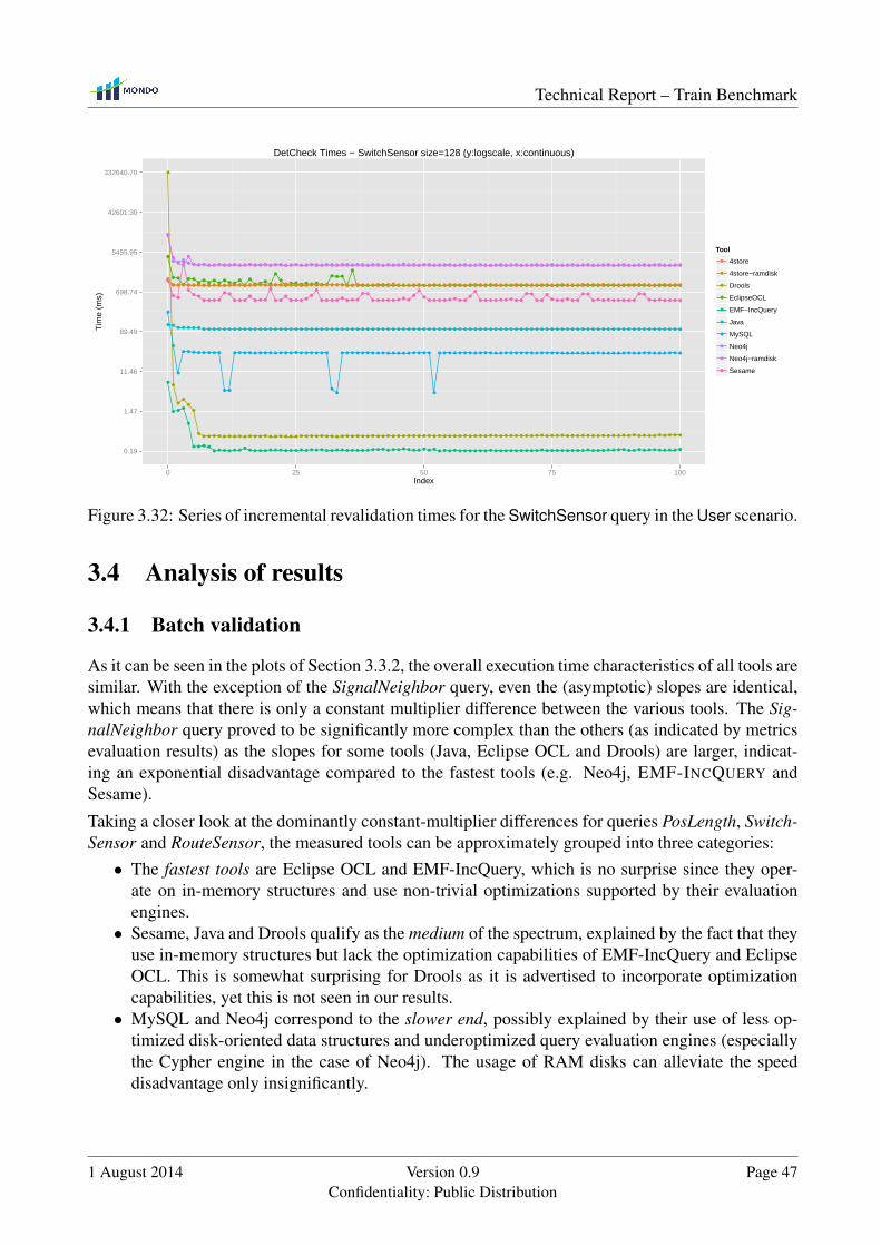
Technical Report – Train Benchmark
●
●
●
●
●●
●
●●●
●
●
●
●
●●
●
●●
●
●
●
●
●
●●
●
●●
●
●
●
●
●
●
●
●
●●
●
●
●
●
●
●
●
●
●●●
●
●
●
●
●●
●
●●
●
●
●
●
●
●●
●
●●
●
●
●
●
●
●●
●
●●
●
●
●
●
●
●●
●
●●
●
●
●
●
●
●●
●
●●
●
●
●
●
●
●●
●
●●
●
●
●
●
●
●●
●
●●
●
●
●
●
●
●●
●
●●
●
●
●
●
●
●●
●
●●
●
●
●
●
●
●●
●
●●
●
●
●
●
●
●●
●
●●
●
●
●
●
●
●●
●
●●
●
●
●
●
●
●●
●
●●
●
●
●
●
●
●●
●
●●
●
●
●
●
●
●●
●
●●
●
●
●
●
●
●●
●
●●●
●
●
●
●
●●
●
●●
●
●
●
●
●
●●
●
●●
●
●
●
●
●
●●
●
●●
●
●
●
●
●
●●
●
●●
●
●
●
●
●
●●
●
●●
●
●
●
●
●
●●
●
●●
●
●
●
●
●
●●
●
●●
●
●
●
●
●
●●
●
●●
●
●
●
●
●
●●
●
●●
●
●
●
●
●
●●
●
●●
●
●
●
●
●
●●
●
●●
●
●
●
●
●
●●
●
●●
●
●
●
●
●
●●
●
●●
●
●
●
●
●
●●
●
●●
●
●
●
●
●
●●
●
●●
●
●
●
●
●
●●
●
●●
●
●
●
●
●
●●
●
●●
●
●
●
●
●
●●
●
●●
●
●
●
●
●
●●
●
●●
●
●
●
●
●
●●
●
●●
●
●
●
●
●
●●
●
●●
●
●
●
●
●
●●
●
●●
●
●
●
●
●
●●
●
●●
●
●
●
●
●
●●
●
●●
●
●
●
●
●
●●
●
●●
●
●
●
●
●
●●
●
●●
●
●
●
●
●
●●
●
●●
●
●
●
●
●
●●
●
●●
●
●
●
●
●
●●
●
●●
●
●
●
●
●
●●
●
●●
●
●
●
●
●
●●
●
●●
●
●
●
●
●
●●
●
●●
●
●
●
●
●
●●
●
●●
●
●
●
●
●
●●
●
●●
●
●
●
●
●
●●
●
●●
●
●
●
●
●
●●
●
●●
●
●
●
●
●
●●
●
●●
●
●
●
●
●
●●
●
●●
●
●
●
●
●
●●
●
●●
●
●
●
●
●
●●
●
●●
●
●
●
●
●
●●
●
●●
●
●
●
●
●
●●
●
●●
●
●
●
●
●
●●
●
●●
●
●
●
●
●
●●
●
●●
●
●
●
●
●
●●
●
●●
●
●
●
●
●
●●
●
●●
●
●
●
●
●
●●
●
●●
●
●
●
●
●
●●
●
●●
●
●
●
●
●
●●
●
●●
●
●
●
●
●
●●
●
●●
●
●
●
●
●
●●
●
●●
●
●
●
●
●
●●
●
●●
●
●
●
●
●
●●
●
●●
●
●
●
●
●
●●
●
●●
●
●
●
●
●
●●
●
●●
●
●
●
●
●
●●
●
●●
●
●
●
●
●
●●
●
●●
●
●
●
●
●
●●
●
●●
●
●
●
●
●
●●
●
●●
●
●
●
●
●
●●
●
●●
●
●
●
●
●
●●
●
●●
●
●
●
●
●
●●
●
●●
●
●
●
●
●
●●
●
●●
●
●
●
●
●
●●
●
●●
●
●
●
●
●
●●
●
●●
●
●
●
●
●
●●
●
●●
●
●
●
●
●
●●
●
●●
●
●
●
●
●
●●
●
●●
●
●
●
●
●
●●
●
●●
●
●
●
●
●
●●
●
●●
●
●
●
●
●
●●
●
●●
●
●
●
●
●
●●
●
●●
●
●
●
●
●
●●
●
●●
●
●
●
●
●
●●
●
●●
●
●
●
●
●
●●
●
●●
●
●
●
●
●
●●
●
●●
●
●
●
●
●
●●
●
●●
●
●
●
●
●
●●
●
●●
●
●
●
●
●
●●
●
●●
●
●
●
●
●
●●
●
●●
●
0.19
1.47
11.46
89.49
698.74
5455.95
42601.30
332640.70
0 25 50 75 100Index
Tim
e (m
s)
Tool
●
●
●
●
●
●
●
●
●
●
4store
4store−ramdisk
Drools
EclipseOCL
EMF−IncQuery
Java
MySQL
Neo4j
Neo4j−ramdisk
Sesame
DetCheck Times − SwitchSensor size=128 (y:logscale, x:continuous)
Figure 3.32: Series of incremental revalidation times for the SwitchSensor query in the User scenario.
3.4 Analysis of results
3.4.1 Batch validation
As it can be seen in the plots of Section 3.3.2, the overall execution time characteristics of all tools aresimilar. With the exception of the SignalNeighbor query, even the (asymptotic) slopes are identical,which means that there is only a constant multiplier difference between the various tools. The Sig-nalNeighbor query proved to be significantly more complex than the others (as indicated by metricsevaluation results) as the slopes for some tools (Java, Eclipse OCL and Drools) are larger, indicat-ing an exponential disadvantage compared to the fastest tools (e.g. Neo4j, EMF-INCQUERY andSesame).
Taking a closer look at the dominantly constant-multiplier differences for queries PosLength, Switch-Sensor and RouteSensor, the measured tools can be approximately grouped into three categories:• The fastest tools are Eclipse OCL and EMF-IncQuery, which is no surprise since they oper-
ate on in-memory structures and use non-trivial optimizations supported by their evaluationengines.• Sesame, Java and Drools qualify as the medium of the spectrum, explained by the fact that they
use in-memory structures but lack the optimization capabilities of EMF-IncQuery and EclipseOCL. This is somewhat surprising for Drools as it is advertised to incorporate optimizationcapabilities, yet this is not seen in our results.• MySQL and Neo4j correspond to the slower end, possibly explained by their use of less op-
timized disk-oriented data structures and underoptimized query evaluation engines (especiallythe Cypher engine in the case of Neo4j). The usage of RAM disks can alleviate the speeddisadvantage only insignificantly.
1 August 2014 Version 0.9Confidentiality: Public Distribution
Page 47

Technical Report – Train Benchmark
IncQuery vs. OCL specific observations. From the batch query evaluation of the PosLength,SwitchSensor and RouteSensor queries (Section 3.3.2), it can be seen that EMF-INCQUERY per-forms similarly to Eclipse OCL. It is slightly faster for small models (2 s and 3 s respectively), butis slower for large models (up to 125 s and 78 s), where this 50% slowdown (once in the wholescenario) can be attributed to the initial (Rete) cache build.
However, for the more complex SignalNeighbor query, it is observed that EMF-INCQUERY outper-forms Eclipse OCL by a large margin solutions: it is noticeably faster for small modells (2 s and 4 s),and over 435k model elements OCL did not finish with the initial analysis in 12 minutes. This per-formance gain might be attributed to the more efficient (cached) enumeration of instances, and thepossibility of backward navigation (with the help of auxiliary structures) on unidirectional referencesused by this query.
3.4.2 Incremental revalidation
As designed, this phase illustrates the characteristic difference between traditional, “batch” queryengines and incremental tools clearly. Total revalidation time (shown on the X axis in the plotsof Section 3.3.3) corresponds to the execution time of editing and re-checking operations, i.e. itapproximates an incremental model transformation sequence for incremental tools and a batch trans-formation + batch query evaluation sequence for traditional tools.
The characteristic advantage of incremental tools (i.e. EMF-INCQUERY and Drools) is best seenon the Y axes of the plots, as these tools are typically 1-2 orders of magnitude (i.e. 10 to 100times) faster than the rest. Since the plots include editing and result retrieval operations that scalelinearly with model size, the overall low-order polynomial characteristics apply to all of the tools.The SignalNeighbor query again highlights EMF-INCQUERY’s clear advantage when dealing withvery complex queries: it beats all other tools by 3-5 orders of magnitude.
3.4.3 Highlights of interest
Differences between the User and Xform scenarios. As noted in Section 2.1.5, the main differ-ence between the User and Xform scenarios is the amount of model manipulation operations, whichis significantly larger for the Xform scenario. The query result sets are also larger for the Xform sce-nario. By comparing corresponding plots, it is observed that the overall evaluation time is affectedlinearly by this difference (explained by the specification which requires a complete reading throughthe entire result list), meaning that all tools are capable of handling this efficiently.
Execution time differences can be huge. While the overall characteristics of all tools are similar(low order polynomial with a constant component), we have recorded a rather large variation ofexecution times (0.5-4 orders of magnitude difference). This confirms our expectation that modelpersistence, (de)serialization, query evaluation and model transformation technologies can have ahuge overall impact on MDE performance.
Page 48 Version 0.9Confidentiality: Public Distribution
1 August 2014

Technical Report – Train Benchmark
RAM disks matter less than anticipated. Some measurements using 4store and Neo4j were per-formed with both SSD-based and RAMdisk-based storage backends. Overall, as it is seen from totaltime measurements (Section 3.3.4), RAMdisk-based variants were about twice as fast – which is lessthan we originally anticipated.
Hand-coded Java and MySQL are surprisingly fast in some cases. We created the hand-codedJava and MySQL implementations as baselines to which more sophisticated tools can be measured.While the advanced tools are the clear winners overall, the Java and MySQL baselines were surpris-ingly fast in several configurations. We interpret this as a sign that more sophisticated tools, andspecifically MDE technologies still have a lot of performance enhancement potential to be unlocked.
JIT HotSpot optimizations kick in late. As seen in Section 3.3.5 and even better in Section 3.3.6,the execution time for certain operations executed in cycles can decrease dramatically over time. Inthe Java Runtime environment, this effect is best explained by Just-in-time (HotSpot) compiling bythe Java Virtual Machine. Overall, it can be concluded that at least 30-50 complex operation iterationsare advised to be executed in a benchmarking environment to obtain results that are relevant to longrunning software.
3.4.4 Threats to Validity
Internal threats
Mitigating measurement risks. We tried to mitigate internal validity threats by reducing the num-ber of uncontrolled variables during measurements: a physical machine was used with all unnec-essary software components turned off and every execution was isolated into a freshly initializedJVM.
Ensuring functional equivalence and correctness. The queries are semantically equivalent in thedifferent query languages and the result sets are the same for every model. Our current measure-ments only loaded and executed a single query in each run. When loading multiple queries, queryinterference may change the results greatly. A more detailed evaluation of this issue is planned forthe future.
Code reviews. Additionally, to ensure comparable results the created high-quality query imple-mentations were reviewed: the OCL implementation by Ed Willink from the Eclipse OCL project,the usage of Impact Analyzer by Axel Uhl from the Impact Analyzer developer team. The graphpatterns were written by the developers of EMF-INCQUERY. SPARQL code was reviewed by asemantic web expert. Drools rules were reviewed by the JBoss Drools developer team.
1 August 2014 Version 0.9Confidentiality: Public Distribution
Page 49

Technical Report – Train Benchmark
External threats
Metrics and generalizability of results. Considering external validity, the generalization of theresults largely depends on how representative the metamodels, the models and the queries are com-pared to real use cases. In section 2.2 metrics were defined to describe complexity of models andqueries, however comparing them to real world ones remains a future work.
Industrial relevance. The metamodel and the query specifications were motivated by an industrialcase study, and the selected queries feature commonly used validation tasks such as attribute andreference checks or cycle detection. We tried to ensure that the instance models have a similarstructure and distribution to other models by parameterizing the generation process based on ourexperience with other domains. To summarize, we believe that the train domain and the generatedinstance models represent other domain-specific languages and available instance models well.
3.5 Evaluation of Metrics
3.5.1 Method of Analysing Metrics
Our long-term goal is providing a catalog of reliable benchmark data that, based on metrics of themodel and the queries, will allow the engineer to extrapolate the expected performance characteristicsof various query technologies, which in turn will support making an informed decision on the solutionto apply. In scope of this paper, we attempt to provide a necessary prerequisite with a narrower focusof investigation: finding out which model and query metrics are useful for predicting the performanceof the various tools, over a wide range of different queries and model structures.
A given metric can only be a useful predictor of a certain performance indicator of a certain toolif they are strongly correlated. Therefore our analysis investigated correlations of metrics and per-formance indicators. Neither previous experience nor current measurement data supported a linearrelationship between these variables; therefore we opted to abandon the commonly used Pearsoncorrelation coefficient that is associated with linear regression. We rely instead on Kendall’s τ rankcorrelation coefficient, ranging from –1 to +1; without assuming a linear model, τ characterises thedegree to which it can be said that larger values of the metric correspond to larger values of theperformance indicator.
Correlation coefficients may lead to incorrect conclusions if the sample of models and queries istoo small. Therefore, whenever measuring an absolute value of τ , we additionally conducted theassociated statistical test (τ -test) to decide whether the detected correlation between the variables isstatistically significant (p < 0.001). Note that any such statistical result is conditional to the uniformsampling of the selected queries and models.
A limitation of the approach is that two strongly correlated variables (e.g. countEdges andcountTriples) may show up as equally good predictors, but in reality they can not be usedas two independent signals for predicting performance (as most triples in our models are edges). Thesimple correlation-based analysis presented here is intended as preliminary feature selection; we in-tend to follow up with redundancy-reducing feature selection techniques such as mRMR [25] that
Page 50 Version 0.9Confidentiality: Public Distribution
1 August 2014

Technical Report – Train Benchmark
0
0,2
0,4
0,6
0,8
1
countNodes
countEdges
countTriples
avgOutDegree
avgInDegree
maxInDegree
numParameters
numAttrChecks
countMatches
selectivity
relDifficulty
absDifficulty
Positive
Negative
(a) Java Memory
0
0,2
0,4
0,6
0,8
1
countNodes
countEdges
countTriples
avgOutDegree
avgInDegreecountMatches
selectivity
relDifficulty
absDifficulty
Positive
Negative
(b) Java Read time
0
0,2
0,4
0,6
0,8
1
countNodes
countEdges
countTriples
numParameters
numAttrChecks
nestedNacDepth
countMatches
selectivity
relDifficulty
absDifficulty
Positive
Negative
(c) Java Check time
0
0,2
0,4
0,6
0,8
1
countNodes
countEdges
countTriples
numVariables
numEdgeConstraints
numAttrChecks
nestedNacDepth
countMatches
relDifficulty
absDifficulty
Positive
Negative
(d) EMF-INCQUERY Memory
0
0,2
0,4
0,6
0,8
1
countNodes
countEdges
countTriples
numEdgeConstraints
numAttrChecksnestedNacDepth
countMatches
relDifficulty
absDifficulty
Positive
Negative
(e) EMF-INCQUERY Read time
0
0,2
0,4
0,6
0,8
1
countNodes
countEdges
countTriples
maxInDegree
numParameters
numVariables
numEdgeConstraints
numAttrChecks
nestedNacDepth
countMatches
selectivity
relDifficulty
Positive
Negative
(f) EMF-INCQUERY Check time
0
0,2
0,4
0,6
0,8
1
countNodes
countEdges
countTriples
avgOutDegree
avgInDegree
maxInDegree
numVariables
numAttrChecks
nestedNacDepth
countMatches
relDifficulty
absDifficulty
Positive
Negative
(g) Sesame Memory
0
0,2
0,4
0,6
0,8
1
countNodes
countEdges
countTriples
avgOutDegree
avgInDegree
maxInDegree
numParameters
numVariables
nestedNacDepth
selectivity
relDifficulty
absDifficulty
Positive
Negative
(h) Sesame Read time
0
0,2
0,4
0,6
0,8
1
countNodes
avgOutDegree
avgInDegree
numParameters
numVariablesnumEdgeConstraints
numAttrChecks
countMatches
selectivity
Positive
Negative
(i) Sesame Check time
Figure 3.33: |τ | of correlating (p < 0.001) metrics for each performance indicator.
can take into account which metrics convey independent information. Afterwards, predicting thebest choice of technology based on the metric values is a problem of multivariate regression / classi-fication, for which we plan to employ advanced machine learning techniques (e.g. ID3 [26] decisiontrees or MARS [18] regression model) in future work.
3.5.2 Metrics Colleration Results
For each tool performance indicator and each metric, we conducted Kendall’s correlation test tosee whether the data available is sufficient to form a statistically significant support of correlationbetween the performance indicator and the metric. For metrics that were found to correlate, theabsolute value of Kendall’s τ correlation coefficient is displayed on a spider chart specific to theperformance indicator of the tool (see Figure 3.33); positive correlation values are displayed as redtriangles, while negative ones as blue squares.
1 August 2014 Version 0.9Confidentiality: Public Distribution
Page 51

Technical Report – Train Benchmark
Evaluation
Consistently with previously published results, the data shows that model size is a strong predictorof both model loading time and memory consumption, regardless of the technology.
Tool-specific Observations However, check times show a more diverse picture. The check timesfor the Java implementation (being a dominantly search-intensive approach) are additionally corre-lated with the query-on-model metrics as well, with the strongest correlation shown by the absDiffi-culty metric.
Interestingly, the best Sesame check time predictor turned out to be the number of pattern variables,and there is no significant correlation with any direct model metrics.
Check times in EMF-INCQUERY are very strongly correlated to the number of matches – which isto be expected of an incremental tool whose check phase consists of just enumerating the cachedmatch set. As the incremental indexes are constructed during the load time, the model-on-querymetrics become correlated with EMF-INCQUERY read time. It can also be highlighted that EMF-INCQUERY seems not to be sensitive towards the “difficulty” of the query (in any phase) or the modelsize (during the check phase) due to the very small correlations with corresponding metrics.
Metrics Overall, it can be said that model-only metrics are useful in predicting the performance ofmodel persistence operations. However, query-based and combined metrics (such as our proposedabs- and relDifficulty) are necessary to provide a more thorough picture. Note that since only statis-tically significant correlations are included, a low magnitude correlation does not necessarily mean ameasurement error. It is possible that there is a true link between the two variables, but the τ value islowered by other metrics that strongly influence the performance indicator.
3.5.3 Threats to Validity
Regarding the technological foundations and methodology of our measurements, the most importantthreats to validity stem from time measurement uncertainty and distortions due to transient effectssuch as garbage collection in the JVM and thrashing due to heap size exhaustion. Such effects weremitigated by using the most accurate Java time measurement method (System.nanoTime), al-locating as much heap as possible, and using a timeout mechanism to identify and exclude casesaffected by thrashing from the results. Additionally, it is also possible that there is sampling biasin our choice of models and metrics; we believe that this is sufficiently mitigated by our system-atic choice of model generation strategies and the design principles of the queries. To improve themagnitude of correlation we increased the sample size by running the benchmarks ten times.
Page 52 Version 0.9Confidentiality: Public Distribution
1 August 2014

Chapter 4
Summary
In this tech report, we presented the Train Benchmark, an extensible framework for the definitionand execution of benchmark scenarios for modeling tools. The framework supports the constructionof benchmark test sets that specify the metamodel, instance model generation, queries and transfor-mations, result collection and processing, and metric evaluation logic that are intended to provide anend-to-end solution. Additionally, we also presented a concrete test case set corresponding to the theoriginal Train Benchmark implementation of [31] and its metric-focused extensions in [22].
In addition to the results presented in previous academic papers, the tech report contains a compre-hensive set of measurement results comparing 7 different tools from three technological domains(Ecore, RDF/SPARQL, property graphs). These results allow for intra-domain and inter-domain toolcomparison and detailed execution time characteristics analysis.
As future work, we plan to incorporate further tools (such as Egyed’s OCL Impact Analyzer, Epsilon,ATL, other NoSQL databases using the Tinkerpop API and the Gremlin language). Additionally,work has begun to create a new benchmark case based on source code modernization base study inMONDO.
53
Appendix A
Appendix
A.1 Rete Networks for the Queries of the Train Benchmark
The Rete algorithm uses tuples to represent the vertices (along with their properties), edges andsubgraphs in the graph. The algorithm defines an asynchronous network of communicating nodes.The Rete networks has three layers:
• The top level consists of input nodes which are type-instance indexers for the model. Eachinput node indexes a certain vertex type or edge label. The actual graph element is indicatedby a vertex/edge icon in the upper right corner of the Rete node.• Worker nodes perform a transformation on the output of their parent node(s) and propagate the
results. Partial query results are represented in tuples and stored in the memory of the workernode thus allowing for incremental query reevaluation.• The bottom level consist of production nodes which are terminators that provide an interface
for fetching the results of the query and the changes introduced by the latest transformation.
In Figure A.1–Figure A.4, we present possible Rete networks layouts for the queries in the TrainBenchmark.
54

Technical Report – Train Benchmark
Segment
Seg, length
Production
Term evaluator
length 0
Trimmer [0]
Seg
Figure A.1: The Rete network for thePosLength query.
sensor
TE, Sen Switch
Sw
Production
Antijoin
Sw
0
Trimmer [0]
TE
0
Figure A.2: The Rete network for theSwitchSensor query.
switch
SwP, Sw routeDefinition
R, Sen sensor
Sw, Sen switchPosition
R, SwP
Production
Join
SwP, Sw, R
Join
SwP, Sw, R, Sen
Antijoin
SwP, Sw, R, Sen
0 1
1 0
2, 3 0, 1
Trimmer [2]
R
Figure A.3: The Rete network for the RouteSensor query.
1 August 2014 Version 0.9Confidentiality: Public Distribution
Page 55

Technical Report – Train Benchmark
routeDefinition
R, Sen sensor
TE, Sen
Production node
Trimmer [0]
R
entry
R, Sig exit
R, Sig connectsTo
TE, TE
Join
R, Sig, Sen
0 0
Join
R, Sen, Sig
0 0 0 0
Join
TE, Sen, TE
Join
TE, Sen, TE, Sen
02
Inequality, t[0] t[4]
R, Sen, Sig, Sen, R
Join
R, Sen, Sig, Sen
01
Trimmer [1, 3]
Sen, Sen
Join
R, Sen, Sig, Sen, R
13
Antijoin
R, Sen, Sig, Sen, R
1, 22, 3
Figure A.4: The Rete network for the SignalNeighbor query.
Page 56 Version 0.9Confidentiality: Public Distribution
1 August 2014

Bibliography
[1] Apache Maven. http://maven.apache.org.
[2] MySQL. http://www.mysql.com/.
[3] Neo Technology: Neo4j. http://neo4j.org/.
[4] Redhat Drools Expert. http://www.jboss.org/drools.
[5] Model-based generation of tests for dependable embedded systems, 7th eu framework pro-gramme. http://http://mogentes.eu/, 2011.
[6] The Train Benchmark Website. https://incquery.net/publications/trainbenchmark/full-results, 2013.
[7] The R project for statistical computing. http://www.r-project.org/, 2014.
[8] Thara Angskun, George Bosilca, and Jack Dongarra. Self-healing in binomial graph networks.In Proceedings of the 2007 OTM Confederated international conference on On the move tomeaningful internet systems - Volume Part II, OTM’07, pages 1032–1041, Berlin, Heidelberg,2007. Springer-Verlag.
[9] Albert-László Barabási and Zoltán N. Oltvai. Network biology: understanding the cell’s func-tional organization. Nat Rev Genet, 5(2):101–113, February 2004.
[10] Gábor Bergmann, Ákos Horváth, István Ráth, and Dániel Varró. A benchmark evaluation of in-cremental pattern matching in graph transformation. In Hartmut Ehrig, Reiko Heckel, GrzegorzRozenberg, and Gabriele Taentzer, editors, Proc. 4th International Conference on Graph Trans-formations, ICGT 2008, volume 5214 of Lecture Notes in Computer Science, pages 396–410.Springer, Springer, 2008. Acceptance rate: 40%.
[11] Gábor Bergmann, Ákos Horváth, István Ráth, Dániel Varró, András Balogh, Zoltán Balogh, andAndrás Ökrös. Incremental Evaluation of Model Queries over EMF Models. In Model DrivenEngineering Languages and Systems, 13th International Conference, MODELS’10. Springer,Springer, 10/2010 2010. Acceptance rate: 21%.
[12] Gábor Bergmann, Zoltán Ujhelyi, István Ráth, and Dániel Varró. A Graph Query Languagefor EMF models. In Jordi Cabot and Eelco Visser, editors, Theory and Practice of ModelTransformations, ICMT 2011, volume 6707 of LNCS, pages 167–182. Springer, Springer, 2011.
57

Technical Report – Train Benchmark
[13] Christian Bizer and Andreas Schultz. The Berlin SPARQL benchmark. International Journalon Semantic Web & Information Systems, 5(2):1–24, 2009.
[14] Christian Bizer and Andreas Schultz. The Berlin SPARQL Benchmark. International JournalOn Semantic Web and Information Systems, 5(2), 2009.
[15] Eclipse Model Development Tools Project. Eclispe OCL website, 2011. http://www.eclipse.org/modeling/mdt/?project=ocl.
[16] P. Erdos and A. Rényi. On the evolution of random graphs. Publ. Math. Inst. Hung. Acad. Sci,5:17–61, 1960.
[17] Charles L. Forgy. Rete: A fast algorithm for the many pattern/many object pattern matchproblem. Artificial Intelligence, 19(1):17–37, 1982.
[18] Jerome H. Friedman. Multivariate adaptive regression splines. Ann. Statist., 19(1):1–141, 1991.With discussion and a rejoinder by the author.
[19] Olaf Görlitz, Matthias Thimm, and Steffen Staab. SPLODGE: Systematic generation ofSPARQL benchmark queries for Linked Open Data. In Philippe Cudré-Mauroux, Jeff Heflin,Evren Sirin, Tania Tudorache, Jérôme Euzenat, Manfred Hauswirth, JosianeXavier Parreira,Jim Hendler, Guus Schreiber, Abraham Bernstein, and Eva Blomqvist, editors, The Seman-tic Web – ISWC 2012, volume 7649 of Lecture Notes in Computer Science, pages 116–132.Springer Berlin Heidelberg, 2012.
[20] S. Harris, N. Lamb, and N. Shadbolt. 4store: The design and implementation of a clusteredrdf store. In 5th International Workshop on Scalable Semantic Web Knowledge Base Systems(SSWS2009), 2009.
[21] Benedek Izsó, Gábor Szárnyas, István Ráth, and Dániel Varró. Incquery-d: Incremental graphsearch in the cloud. In Proceedings of the Workshop on Scalability in Model Driven Engineer-ing, BigMDE ’13, pages 4:1–4:4, New York, NY, USA, 2013. ACM.
[22] Benedek Izsó, Zoltán Szatmári, Gábor Bergmann, Ákos Horváth, and István Ráth. Towardsprecise metrics for predicting graph query performance. In 2013 IEEE/ACM 28th InternationalConference on Automated Software Engineering (ASE), pages 412–431, Silicon Valley, CA,USA, 11/2013 2013. IEEE, IEEE.
[23] Benedek Izsó, Zoltán Szatmári, Gábor Bergmann, Ákos Horváth, and István Ráth. Towardsprecise metrics for predicting graph query performance. In 2013 IEEE/ACM 28th InternationalConference on Automated Software Engineering (ASE), pages 412–431, Silicon Valley, CA,USA, 11/2013 2013. IEEE, IEEE. Acceptance Rate: 23%.
[24] Object Management Group. Object Constraint Language Specification (Version 2.3.1), 2012.http://www.omg.org/spec/OCL/2.3.1/.
[25] H. Peng, Fulmi Long, and C. Ding. Feature selection based on mutual information criteria ofmax-dependency, max-relevance, and min-redundancy. Pattern Analysis and Machine Intelli-gence, IEEE Transactions on, 27(8):1226–1238, 2005.
Page 58 Version 0.9Confidentiality: Public Distribution
1 August 2014

Technical Report – Train Benchmark
[26] J. R. Quinlan. Induction of decision trees. Machine Learning, 1(1):81–106, March 1986.
[27] Michael Schmidt, Thomas Hornung, Georg Lausen, and Christoph Pinkel. SP2Bench: ASPARQL performance benchmark. In Proc. of the 25th International Conference on DataEngineering, pages 222–233, Shanghai, China, 2009. IEEE.
[28] Jakub Stárka, Martin Svoboda, and Irena Mlynkova. Analyses of RDF triples in sample datasets.In COLD, 2012.
[29] The Eclipse Project. Eclipse Modeling Framework. http://www.eclipse.org/emf/.
[30] Transaction Processing Performance Council (TPC). TPC-C Benchmark, 2010.
[31] Zoltán Ujhelyi, Gábor Bergmann, Ábel Hegedüs, Ákos Horváth, Benedek Izsó, István Ráth,Zoltán Szatmári, and Dániel Varró. EMF-IncQuery: An Integrated Development Environmentfor Live Model Queries. Science of Computer Programming, 2014. Accepted.
[32] Batagelj Vladimir and Brandes Ulrik. Efficient generation of large random networks. PhysicalReview E, 71(3):036113, 04 2005.
[33] World Wide Web Consortium. Resource Description Framework (RDF). http://www.w3.org/standards/techs/rdf/.
[34] World Wide Web Consortium. SPARQL Query Language for RDF. http://www.w3.org/TR/rdf-sparql-query/.
1 August 2014 Version 0.9Confidentiality: Public Distribution
Page 59