efficiently monitoring reverse k nearest neighbors in ...swan398/paper/hthesis.pdf · school of...
TRANSCRIPT

THE UNIVERSITY OF NEW SOUTH WALESSCHOOL OF COMPUTER SCIENCE AND ENGINEERING
Efficiently MonitoringReverse k Nearest Neighbors
in Spatial Networks
Shenlu Wang( [email protected] )
Computer Science Honours Thesis
Submission Date : 3rd June, 2013Supervisor : Dr. Muhammum Aamir Cheema
Assessor : A.Prof. Wei Wang

Acknowledgements
I would like to thank all those people who have through their support enabled meto complete this thesis.
Firstly, I would like to thank my supervisor Dr. Muhammad Aamir Cheema.He devoted a lot of time throughout my honors year to help me with thesis writing,guild me with literature review, and inspire me with problem solving. He is notjust an expert in his area, but also a very good and kind supervisor.
I would also like to thank Prof. Xuemin Lin. He is the head of databaseresearch group. He contiguously asks me about my progress and encourages meto read more, think more and think deeper.
I would like to thank A.Prof. Wei Wang to be my accessor.I would like to thank the many database research group people for their help
and accompany. They gave me a great and precious memory.Finally, I would like to thank my parents for the various things that made doing
this thesis possible.
i

Abstract
Given a set of clients C, a set of facilities F and a query q ∈ F , a reverse k n-earest neighbors (RkNN) query retrieves every client c ∈ C for which q is oneof the k closest facilities. In the past few years, RkNN queries have received sig-nificant research attention due to its wide range of applications. In this thesis, westudy the problem of continuous monitoring of RkNN queries in road networks.The state-of-the-art technique is sensitive towards the movement of clients, e.g.,whenever a client that is inside the so-called unpruned region changes its loca-tion, the existing technique requires expensive verification of whether the clientis a RkNN of q or not. To address this problem, we utilize the novel concept ofinfluence zone which is a region in the network such that a client c is the RkNNif and only if it lies inside this zone. This significantly improves the performancebecause the problem of continuously monitoring RkNN queries is reduced to theproblem of continuously monitoring the clients that are inside this zone. Based onseveral non-trivial observations, we present an efficient algorithm to compute theinfluence zone. Our extensive experimental study demonstrates that our algorithmis more than an order of magnitude faster than the state-of-the-art algorithm.
ii

Contents
1 Introduction 11.1 Spatial Index . . . . . . . . . . . . . . . . . . . . . . . . . . . . 2
1.1.1 Euclidean Space . . . . . . . . . . . . . . . . . . . . . . 31.1.2 Spatial Network . . . . . . . . . . . . . . . . . . . . . . 4
1.2 Spatial Queries . . . . . . . . . . . . . . . . . . . . . . . . . . . 41.2.1 k Nearest Neighbors Query . . . . . . . . . . . . . . . . 51.2.2 Reverse k Nearest Neighbors Query . . . . . . . . . . . . 61.2.3 Other Query Types . . . . . . . . . . . . . . . . . . . . . 7
1.3 Contributions . . . . . . . . . . . . . . . . . . . . . . . . . . . . 81.4 Thesis Organization . . . . . . . . . . . . . . . . . . . . . . . . . 8
2 Related Work 102.1 Snapshot RkNN Queries in Euclidean Space . . . . . . . . . . . . 10
2.1.1 Pre-Calculation Based Approach . . . . . . . . . . . . . . 112.1.2 FINCH . . . . . . . . . . . . . . . . . . . . . . . . . . . 12
2.2 Snapshot RkNN Queries in Spatial Networks . . . . . . . . . . . 142.2.1 Network Voronoi Diagram . . . . . . . . . . . . . . . . . 14
2.3 Continuous RkNN Queries in Euclidean Space . . . . . . . . . . 162.3.1 Safe Region and Lazy Updates . . . . . . . . . . . . . . . 162.3.2 Influence Zone . . . . . . . . . . . . . . . . . . . . . . . 20
2.4 Continuous RkNN Queries in Spatial Networks . . . . . . . . . . 212.4.1 Multi-way Tree . . . . . . . . . . . . . . . . . . . . . . . 222.4.2 Safe Region, Unpruned and Monitored Network . . . . . 23
iii

CONTENTS iv
3 Overview 273.1 Motivation . . . . . . . . . . . . . . . . . . . . . . . . . . . . . . 273.2 Problem Formulation . . . . . . . . . . . . . . . . . . . . . . . . 293.3 Solution Overview . . . . . . . . . . . . . . . . . . . . . . . . . 31
4 Influence Zone Based Techniques 334.1 Terms and Notations . . . . . . . . . . . . . . . . . . . . . . . . 334.2 Properties . . . . . . . . . . . . . . . . . . . . . . . . . . . . . . 344.3 Identifying Inner Nodes and Bounding Nodes . . . . . . . . . . . 364.4 Calculating Inner Edges and Inner Segments . . . . . . . . . . . . 38
4.4.1 Handling Monotonic Edges . . . . . . . . . . . . . . . . 394.4.2 Handling Non-monotonic Edges . . . . . . . . . . . . . . 43
4.5 Extension to Directed Graph . . . . . . . . . . . . . . . . . . . . 444.6 Monitoring Phase . . . . . . . . . . . . . . . . . . . . . . . . . . 46
5 Experiments 485.1 Experimental Settings . . . . . . . . . . . . . . . . . . . . . . . . 485.2 Influence Zone Size . . . . . . . . . . . . . . . . . . . . . . . . . 495.3 Running Time . . . . . . . . . . . . . . . . . . . . . . . . . . . . 505.4 Calculating Influence Zone . . . . . . . . . . . . . . . . . . . . . 52
6 Concluding Remark 546.1 Conclusion . . . . . . . . . . . . . . . . . . . . . . . . . . . . . 546.2 Future Work . . . . . . . . . . . . . . . . . . . . . . . . . . . . . 55

List of Figures
1.1 Gas stations near The University of New South Wales. . . . . . . 21.2 Reverse k Nearest Neighbors Query . . . . . . . . . . . . . . . . 6
2.1 Search Region and Candidate Region . . . . . . . . . . . . . . . 132.2 Network Voronoi Diagram . . . . . . . . . . . . . . . . . . . . . 152.3 The exact location of q on MN is unknown. . . . . . . . . . . . . 182.4 Approximation of parabola. . . . . . . . . . . . . . . . . . . . . . 182.5 Half-space Pruning and Dominance Pruning. . . . . . . . . . . . 192.6 Pruned area if exact location of query is known . . . . . . . . . . 202.7 Grid Based Index of Influence Zone . . . . . . . . . . . . . . . . 212.8 PMR Quad-tree . . . . . . . . . . . . . . . . . . . . . . . . . . . 222.9 Monitoring Area. . . . . . . . . . . . . . . . . . . . . . . . . . . 232.10 Monitored Network . . . . . . . . . . . . . . . . . . . . . . . . . 26
3.1 Illustration of RkNN queries . . . . . . . . . . . . . . . . . . . . 303.2 A simple spatial network example. . . . . . . . . . . . . . . . . . 32
4.1 Influence zone Z1 (k = 1) . . . . . . . . . . . . . . . . . . . . . . 384.2 Influence zone Z2 (k = 2) . . . . . . . . . . . . . . . . . . . . . . 414.3 Inner segment is the segment pruned by less than k facilities. . . . 424.4 Handling non-monotonic edge. . . . . . . . . . . . . . . . . . . . 434.5 A simple directed spatial network example. . . . . . . . . . . . . 454.6 Index of influence zones. . . . . . . . . . . . . . . . . . . . . . . 46
5.1 Influence zone size. . . . . . . . . . . . . . . . . . . . . . . . . . 495.2 Total running time. . . . . . . . . . . . . . . . . . . . . . . . . . 50
v

LIST OF FIGURES vi
5.3 Total running time. . . . . . . . . . . . . . . . . . . . . . . . . . 515.4 Total running time. . . . . . . . . . . . . . . . . . . . . . . . . . 515.5 Influence zone calculation phase CPU time cost. . . . . . . . . . . 52

List of Tables
4.1 Notations . . . . . . . . . . . . . . . . . . . . . . . . . . . . . . 33
5.1 System Parameters for Experiments . . . . . . . . . . . . . . . . 49
vii
Chapter 1
Introduction
Spatial database has been an active research area for more than three decades, s-tudying the problems of management and query needs for spatial applications suchas Geographic Information Systems (GIS). Other applications include ComputerAided Design (CAD), Very-Large-Scale Integration (VLSI) design, and Multime-dia Information System (MMIS). The current research is aiming at improving thefunctionality and performance of spatial database management systems.
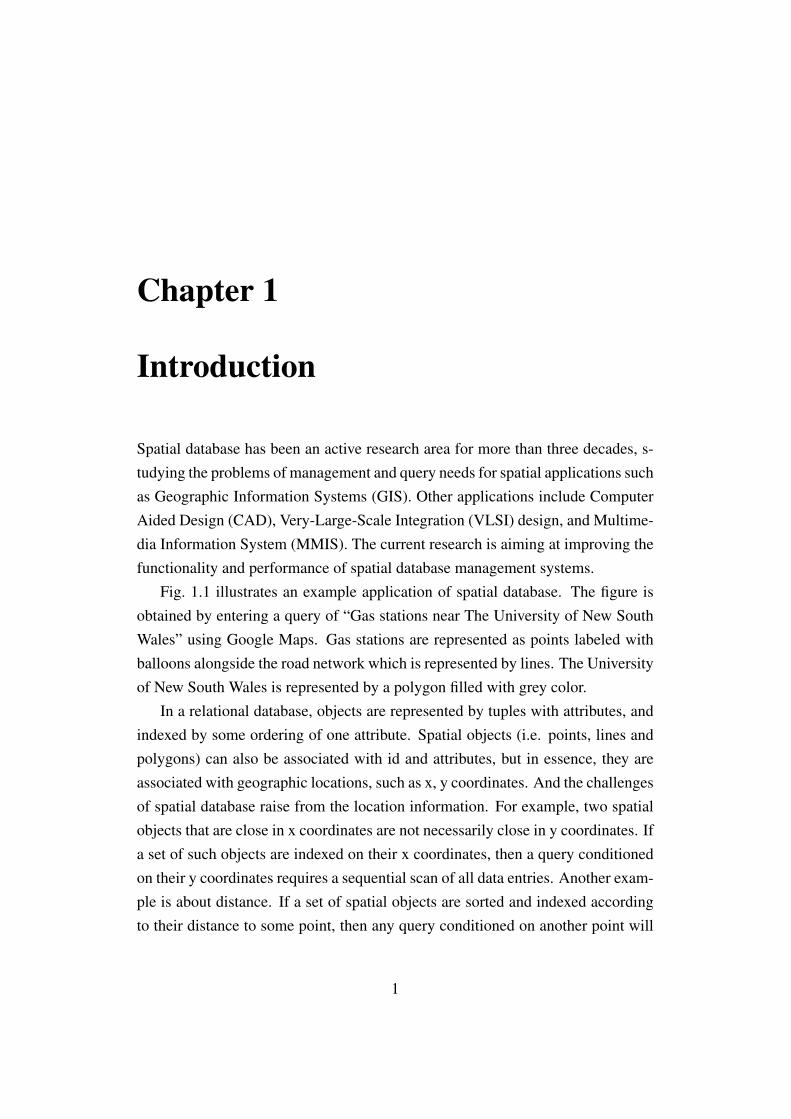
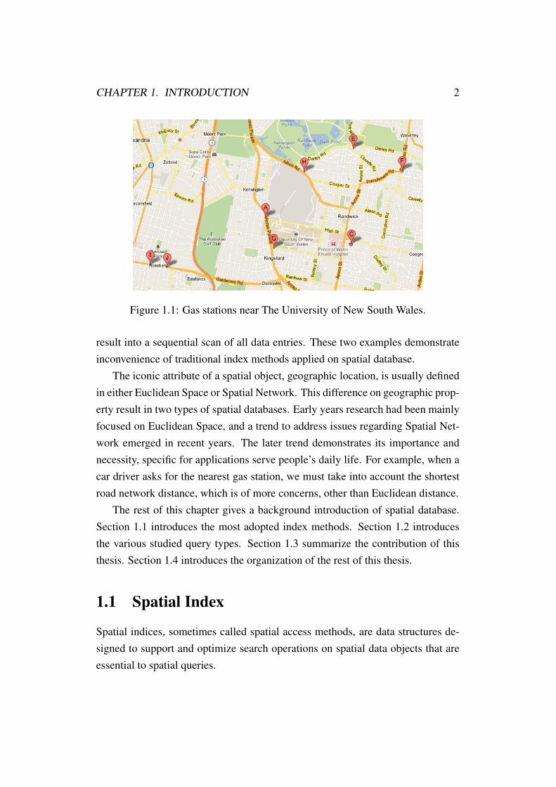
Fig. 1.1 illustrates an example application of spatial database. The figure isobtained by entering a query of “Gas stations near The University of New SouthWales” using Google Maps. Gas stations are represented as points labeled withballoons alongside the road network which is represented by lines. The Universityof New South Wales is represented by a polygon filled with grey color.
In a relational database, objects are represented by tuples with attributes, andindexed by some ordering of one attribute. Spatial objects (i.e. points, lines andpolygons) can also be associated with id and attributes, but in essence, they areassociated with geographic locations, such as x, y coordinates. And the challengesof spatial database raise from the location information. For example, two spatialobjects that are close in x coordinates are not necessarily close in y coordinates. Ifa set of such objects are indexed on their x coordinates, then a query conditionedon their y coordinates requires a sequential scan of all data entries. Another exam-ple is about distance. If a set of spatial objects are sorted and indexed accordingto their distance to some point, then any query conditioned on another point will
1
CHAPTER 1. INTRODUCTION 2
Figure 1.1: Gas stations near The University of New South Wales.
result into a sequential scan of all data entries. These two examples demonstrateinconvenience of traditional index methods applied on spatial database.
The iconic attribute of a spatial object, geographic location, is usually definedin either Euclidean Space or Spatial Network. This difference on geographic prop-erty result in two types of spatial databases. Early years research had been mainlyfocused on Euclidean Space, and a trend to address issues regarding Spatial Net-work emerged in recent years. The later trend demonstrates its importance andnecessity, specific for applications serve people’s daily life. For example, when acar driver asks for the nearest gas station, we must take into account the shortestroad network distance, which is of more concerns, other than Euclidean distance.
The rest of this chapter gives a background introduction of spatial database.Section 1.1 introduces the most adopted index methods. Section 1.2 introducesthe various studied query types. Section 1.3 summarize the contribution of thisthesis. Section 1.4 introduces the organization of the rest of this thesis.
1.1 Spatial Index
Spatial indices, sometimes called spatial access methods, are data structures de-signed to support and optimize search operations on spatial data objects that areessential to spatial queries.

CHAPTER 1. INTRODUCTION 3
Widely used index methods in relational databases, such as B-tree [3, 2], ex-tendible hashing [13] and linear hashing [24], are one dimensional access methodshence not suitable for spatial database simply because the search space is multidi-mensional.
1.1.1 Euclidean Space
R-tree [16], proposed by Antonin Guttman in 1984, is the mostly used indexingmethod to optimize spatial query in Euclidean Space.
In a R-tree, objects are represented by intervals in multiple dimensions. Andthe key idea of R-tree is to group nearby objects and index them using their min-imum bounding rectangle. In this way, a search for objects is reduced to a searchof intersection bounding rectangles. Intersection with a higher level boundingrectangle requires exploring of sub-tree, or, in the other hand, results in a prunedsub-tree.
Compared with traditional indexing methods, R-tree has several advantages tobe applied in a spatial context.
• Unlike hash based indexing methods, which support exact match efficiently,R-tree supports range query in addition.
• Unlike one dimensional ordering of a single key value provided by B-tree,R-tree provides two dimensional ordering, and can be extended easily tohigher dimensional space.
• Unlike Grid indexing, where cells shall be decided in advance, R-tree usesminimum bounding rectangles that can be updated dynamically.
• Unlike Quad tree and k-d tree, R-tree takes into account also I/O cost ofsecondary memory.
Due to the significant use in both theoretical and practical contexts, many vari-ations have been proposed, trying to make it more efficient or trying to improveits worst case performance, such as R*-tree [15], R+-tree [40], Hilbert R-tree [18]and Priority R-tree [1].

CHAPTER 1. INTRODUCTION 4
Another interesting extension is Vor-Tree [41], which incorporates Voronoidiagram into R-tree. The hierarchical structure of R-tree allows search quickly ar-rive the right neighborhood. And the Voronoi diagram provides a tighter polygonshaped search region contrasts with coarser rectangular search region.
1.1.2 Spatial Network
Spatial network can be modeled as a graph, and therefore indices for graph can beused to index spatial networks (i.e. adjacency matrix and adjacency list). Sincethey are well known to the community, the details are omitted.
Although spatial network is gaining more serious attention in recent years,there is a lack of significant research into its indexing technologies.
Shortest path quadtree [36] is an interesting indexing method. It encodes allpair’s shortest path information based on an observation that the shortest path froma vertex to all remaining vertices can be grouped according to the first edges onthe shortest paths to them. Shortest path quadtree captures this spatial coherenceand reduces the storage requirement as only the first edge along the shortest pathsare stored. A search for a shortest path over shortest path quadtree can thereby bereduced to recursively retrieving the first edge to the next vertex along the shortestpath.
Shortest path quadtree takes advantage of the observation that shortest paths inroad networks are spatially coherent. Apart from [36], [37, 39, 38] also take thisadvantage. Another important observation is that some vertices in a road networkare more important than other vertices [14, 30].
Contraction Hierarchies (CH) [14] utilize the second observation and imposesa total ordering on the vertices according to their relative importance. [30] is anextension to CH.
1.2 Spatial Queries
Various query types were formulated and proposed to adapt to different occasions.This section briefly describes a few of them. And most of all, the closely related
CHAPTER 1. INTRODUCTION 5
query types (i.e. k nearest neighbors query and reverse k nearest neighbors query)are introduced with more detailed description.
1.2.1 k Nearest Neighbors Query
Nearest neighbor query is one of the most fundamental research problem in thearea of spatial database. Given a query point q, and a set of spatial objects, near-est neighbor query finds the closest object to the query point according to somedistance metric. Similarly, k nearest neighbors (kNN) query [32] finds the first kclosest objects to the query point. NN query is a special case of kNN query, wherek = 1. More specifically, any object which is not a kNN of the query point, hasdistance to query greater than distance from any of the kNN to the query.
This problem is well studied, and includes several variants, such as continuousnearest neighbor query [26], aggregate nearest neighbor query, and path nearestneighbor query [10].
An example of kNN query could be “find out the 5 closest soldiers” issuedby a nurse in a battle field. In this case, the distance is better measured by theEuclidean distance. Another example of kNN query could be “find out the 3closest gas stations” asked by a car driver. In this case, the distance is bettermeasured by the shortest road network distance.
Since kNN query are extensively studied, hence several variants emerged.Each variant targets a particular problem setting, and adds different requirementsto the supporting indexing method.Snapshot k Nearest Neighbor Query Snapshot query targets static data set,where all the spatial objects as well as query point are static. This type of querygenerally does not update the underlying data structure or at least very rarely.Continuous k Nearest Neighbor Query Continuous k nearest neighbor queryreport kNN for a query point over a time period. The problem arise when either thequery point or other objects are constantly updating their location. The databaseis not static, and hence requires frequent updating. This type of query is mostrelated to this thesis.Approximate k Nearest Neighbor Query Sometimes finding exact kNN is notnecessary or even not feasible, especially when the data set is huge or in a data

CHAPTER 1. INTRODUCTION 6
stream where information can only be accessed once. In these case, many solu-tions to find the approximate kNN were proposed.Distributed Processing of k Nearest Neighbor Query Apart from a central serv-er, this type of query take into account other computational modules as well. Forexample, if the computation and data storage can be distributed to smart phones,and utilize the CPU and storage unite on these mobile devices, the computationalload on the server can be reduced, with a potential to reduce communication cost,which is also very expensive in such a system.
1.2.2 Reverse k Nearest Neighbors Query
Reverse k nearest neighbors (RkNN) query is a very important variant of kNNquery, and it is the topic of this thesis.
A RkNN query finds out a set of objects, not necessarily k objects, where thequery point is kNN of any object in the set. This naturally captures the objectsthat influenced the most by the query point, hence have various applications inlocation based services include location based games, traffic monitoring, locationbased SMS advertising, market analysis, enhanced 911 services and army strategicplanning etc. These applications may require continuous monitoring of reversenearest moving clients.
Figure 1.2: Reverse k Nearest Neighbors Query
As illustrated in Fig. 1.2, there are two gas stations, f1 and f2, and there aretwo cars, c1 and c2. Assume f2 is the query point. The nearest neighbor of f2 isc1 since c1 is closer to f2 than c2, but the reverse nearest neighbor of f2 is c2 sincethe nearest neighbor of c2 is f2 but the nearest neighbor of c1 is not f2.
Although c1 is the nearest neighbor of f2, but since the nearest gas station ofc1 is f1 and the nearest gas station of c2 is f2, hence f2 has a higher influence on

CHAPTER 1. INTRODUCTION 7
c2 than c1. Assume both c1 and c2 would like to go to their nearest gas station andrefuel, then c1 prefers f1 and c2 prefers f2.
The owner of the gas station f2 may want to continuously monitor its RkNNcars and may decide to send them promotional offers. Such promotional offersare expected to influence car drivers more than promotional offers send to its kNNcars.
1.2.3 Other Query Types
Optimal Location Query Optimal location (OL) query is particularly useful forstrategic planning of resources [51]. Given a set of facilities, a set of clients and aset of candidate locations, an optimal location query finds out the candidate loca-tion which optimize a certain cost metric. For example, a city government plansto build a new hospital (i.e. a new facility). Given the locations of all the existinghospitals (i.e. a set of facilities), the government may seek a candidate locationthat minimize distance from any resident (i.e. client) to its nearest hospital.Top-k Spatial Keyword Query Given a set of spatial objects with textual descrip-tion, a query point with search keywords, a top-k spatial keyword query seeks thehighest ranked k objects in terms of both spatial and textual similarity of thoseobjects with the query [31]. For example, a user may want to find out the nearest5 restaurants that serve Italian or French foods. A good index to assist this kindof query may be a combination of R-tree and inverted index.Maximizing Range Sum Query Given a set of weighted points, maximizingrange sum query finds out a rectangular or circular location of given size suchthat the sum of the weights of all covered points is the maximum possible [12].For example, a coffee chain holds some data about their members, including theirhome address and how often they would love to have a cup of coffee in store with-in a limited distance. Then the manager may want to issue a maximizing rangesum query to find out the most profitable location to open a new site.
CHAPTER 1. INTRODUCTION 8
1.3 Contributions
With the popularity of cheap mobile devices, continuously monitoring of spatialqueries over moving objects became an important issue to many location-basedservices and applications.
RkNN query is of significant concern due to its natural capturing of the in-fluence of the query point, hence can have many applications such as decisionsupport, location based services, resource allocation, profile-based management,etc.
This thesis focuses on the problem of efficiently monitoring of reverse k near-est neighbor query in spatial network. The contributions can be summarized asfollows.
• We are the first to study the influence zone in road networks that have ap-plications in RkNN queries, marketing and decision making. We proposean efficient influence zone computation algorithm based on several novelobservations and pruning rules.
• We demonstrate the usefulness of influence zone by developing an efficien-t algorithm to continuously monitor reverse k nearest neighbor queries inspatial networks. Our techniques can be applied to both directed and undi-rected networks.
• We conduct extensive experimental study and demonstrate that our contin-uous RkNN monitoring algorithm is more than an order of magnitude moreefficient than the state-of-the-art algorithm.
1.4 Thesis Organization
The rest of this thesis is organized as follows.
• Chapter 2 summarizes a few most related works about snapshot RkNNquery and continuous RkNN query in both Euclidean Space and SpatialNetwork.

CHAPTER 1. INTRODUCTION 9
• Chapter 3 presents an overview of our solution, includes the motivation be-hind this thesis, a formal definition of the thesis problem (i.e. continuouslymonitoring RkNN query in spatial network), and followed by the outline ofour solution.
• Chapter 4 presents our influence zone computation algorithm that based onseveral novel observations and pruning rules and discusses the monitoringphase where the influence zone is to be used to efficiently monitor continu-ous RkNN query.
• Chapter 5 provides an extensive experimental study using a real word roadnetwork with various settings of several parameters, and shows that the p-resented algorithm more than an order of magnitude more efficient than thestate-of-the-art algorithm.
• Chapter 6 concludes this thesis and explores remaining problems and po-tential future works.

Chapter 2
Related Work
This chapter examines related work on snapshot RkNN query and continuousmonitoring of RkNN query in both Euclidean Space and Spatial Network. In-fluential works are introduced with a summary of their advantages and disadvan-tages, including the reason why they are not applicable for the problem studiedthrough this thesis. Two representative works from each section are described indetail.
2.1 Snapshot RkNN Queries in Euclidean Space
RNN queries were first introduced by Korn et. al [22] who answer the RNN queryby using preprocessing. Specifically, for each data object p, they pre-calculate itsnearest neighbor and assign a circle for p such that p is the center of the circle andthe distance to its nearest neighbor is the radius. Then, RNN of a query q can becomputed by returning every point that contains q in its circle. Yang et. al [52]and Lin et. al [23] present techniques to improve the work done in [22]. [22] isexplained in detail in Section 2.1.1.
Stanoi et. al [42] handle RkNN queries by partitioning the space centered atthe query point q into six regions of 60 degrees each. It can be proved that, foreach partition, any client that is further from query than the kth closest facility of qcannot be the RkNN of q. They utilize this observation to prune the search space.
Cheema et. al [6, 8] introduce the concept of influence zone for answering
10
CHAPTER 2. RELATED WORK 11
reverse k nearest neighbors queries. To compute the RkNN queries, initially theinfluence zone is computed then each client that lies inside the influence zone isreturned as answer. As stated earlier, their work is only applicable to Euclideanspace and it is non-trivial to extend the techniques for road networks.
Sharifzadeh et. al [41] introduced an index structure VoR-tree to efficientlyanswer various spatial queries including reverse k nearest neighbors queries.
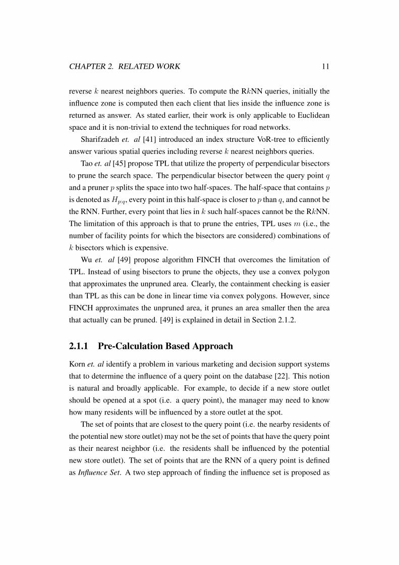
Tao et. al [45] propose TPL that utilize the property of perpendicular bisectorsto prune the search space. The perpendicular bisector between the query point qand a pruner p splits the space into two half-spaces. The half-space that contains pis denoted as Hp:q, every point in this half-space is closer to p than q, and cannot bethe RNN. Further, every point that lies in k such half-spaces cannot be the RkNN.The limitation of this approach is that to prune the entries, TPL uses m (i.e., thenumber of facility points for which the bisectors are considered) combinations ofk bisectors which is expensive.
Wu et. al [49] propose algorithm FINCH that overcomes the limitation ofTPL. Instead of using bisectors to prune the objects, they use a convex polygonthat approximates the unpruned area. Clearly, the containment checking is easierthan TPL as this can be done in linear time via convex polygons. However, sinceFINCH approximates the unpruned area, it prunes an area smaller then the areathat actually can be pruned. [49] is explained in detail in Section 2.1.2.
2.1.1 Pre-Calculation Based Approach
Korn et. al identify a problem in various marketing and decision support systemsthat to determine the influence of a query point on the database [22]. This notionis natural and broadly applicable. For example, to decide if a new store outletshould be opened at a spot (i.e. a query point), the manager may need to knowhow many residents will be influenced by a store outlet at the spot.
The set of points that are closest to the query point (i.e. the nearby residents ofthe potential new store outlet) may not be the set of points that have the query pointas their nearest neighbor (i.e. the residents shall be influenced by the potentialnew store outlet). The set of points that are the RNN of a query point is definedas Influence Set. A two step approach of finding the influence set is proposed as

CHAPTER 2. RELATED WORK 12
follows.
1. For each data point p, generate a circle (p, dist(p,N(p))), where p is itscenter and dist(p,N(p)) is the distance from p to its nearest neighbor N(p)
as the radius.
2. For any query point q, determine all the circles that contain q, return theircenters.
The proposed approach also tolerates dynamic insertion and deletion of datapoints (note, dynamic does not mean data points are moving). A two step approachfor insertion of a point q is as follows.
1. Determine all the RNN p of q, for each such point p, replace all the circlesof the form (p, dist(p,N(p))) to (p, dist(p, q)).
2. Find the nearest neighbor of q′ of q, and add a circle (q, dist(q,N(q))).
Similarly, deletion of a point q can also be done in two steps, shown as follows.
1. Remove the circle (q, dist(q,N(q))).
2. Determine all the RNN p of q, for each such point p, find its current nearestneighbor N(p), and replace its circle (p, dist(p, q)) to (p, dist(p,N(p))).
Yang et. al [52] and Lin et. al [23] present techniques to improve [22].
2.1.2 FINCH
INCH and FINCH is proposed by Wu et. al in [49]. In contrast with [22], INCHand FINCH do not relay on pre-calculation.
Three steps based on the filter-refinement paradigm is required to processRkNN query. INCH (i.e. INtersections’ Convex Hull) is the first step, whichcomputes a search region where all candidates are inclosed. FINCH (i.e. FastRkNN processing using INCH) is the second step, where the search region isused to find candidates, and discovered candidates are used to gradually tighten

CHAPTER 2. RELATED WORK 13
the search region until no candidate could be found. The last step is a refinementprocess to produce the final result from the set of candidates.
Given the query point q and a data point p, for RNN query (k = 1) the perpen-dicular bisector between them can prune objects in the half-plane that contains p,since all such objects is closer to p than to q. For RkNN query (k > 1), a set ofsuch bisectors can be used to prune objects in a certain area. This is the observa-tion behind INCH and FINCH, and this observation is first introduced by Tao et.
al in their proposed algorithm named TPL [45].But the problem of the observation is that it is computationally expensive when
k > 1. Instead, INCH calculate the convex hull of the region which can not bepruned (candidate region) in that way. The key advantage of using convex hull ofcandidate region is that the filtering process can be done with only one polygonother than many smaller polygons. Fig. 2.1 illustrates the candidate region (blackline) and the search region (red line) for RkNN query when k = 2.
Figure 2.1: Search Region and Candidate Region
FINCH has two parts, namely FINCH-Filter and FINCH-Refine. FINCH-Filter computes a set of candidates, and FINCH-Refine refine the candidate set toproduce the final result. The general case of FINCH-Filter algorithm is an iterativeapproach that starts with an empty set and gradually adds candidate objects to theset and shrinks the search region after each candidate object is identified. A more

CHAPTER 2. RELATED WORK 14
efficient version of FINCH-Filter algorithm is based on R-tree index and followsthe best first search paradigm with respect to their distance from q. FINCH-Refinehas two steps. The first step is efficient but approximate, and the second step iscomputational expensive but precise.
2.2 Snapshot RkNN Queries in Spatial Networks
Spatial queries in spatial networks received significant research attention. Amongthe various query types studied, the shortest path queries [10, 36, 39], kNN queries[11, 21, 20] and range queries [29, 25, 47] are among the most popular ones.
Papadias et. al [29] propose an architecture that integrates network with Eu-clidean space. Base on this architecture, they introduce an approach to utilize Eu-clidean restriction. They also developed a network expansion framework whichprunes search space efficiently.
Safar et. al [35] are the first to propose a solution for snapshot RNN queriesin spatial networks. They use a network Voronoi diagram to process RNN queriesefficiently. In their follow-up work [46], they extend their technique to processRkNN queries in spatial networks. Taniar et. al [44] also study the RNN queriesproblem in spatial network. They use order-2 network Voronoi diagram combinedwith Euclidean distance based lower bound to provide an efficient solution. [35]is explained in detail in Section 2.2.1.
2.2.1 Network Voronoi Diagram
Safar et. al solves RNN query with the aid of Network Voronoi Diagram (NVD)in [35]. Their approach is based on properties of NVD, and their previous work,namely Progressive Incremental Network Expansion (PINE) [33, 34], which fol-lows the incremental network expansion (INE) [29] paradigm.
A Voronoi diagram divides a space into disjoint polygons (i.e. Voronoi cells),where the generator of a polygon is the nearest neighbor of any point inside thepolygon. NVD is defined as graphs. It divides the network into disjoint sub-networks. In a Voronoi diagram, Voronoi cells are of convex polygon shape, butin contrast, Voronoi cells in NVD are of irregular shape. Fig. 2.2 illustrates an

CHAPTER 2. RELATED WORK 15
example network Voronoi diagram.
Figure 2.2: Network Voronoi Diagram
Safar et. al classify RNN into four types depending on if the query point isgenerator or not and interest objects are generators or not. The algorithm is basedon the existence of a NVD accompanied with pre-computed data, such as border-to-border and border-to-generator distances. The four types are listed as follows.
RNNGP (GP ): Both query point and interest objects are generators.
In this case, the candidate interest objects are generators of query adjacent Voronoicells.
RNNGP ( GP ): Only query point is generator.
In this case, the result is the set of interest objects that enclosed by the Voronoicell where the generator is the query point.
RNN GP ( GP ): Both query point and interest objects are not generators.
In this case, the NVD helps reducing network distance calculation time. The ideais to explore the neighborhood of the query point using PINE expansion. And ifan interest object is found, PINE expansion is used to process a NN query of theinterest object to determine if it is the RNN of the query point.

CHAPTER 2. RELATED WORK 16
RNN GP (GP ): Only interest objects are generators.
In this case, the NVD helps reducing network distance calculation time. Theidea is to explore the neighborhood of the query point using network expansion.Generator of the Voronoi cell where the query point belongs to, and the generatorof neighboring Voronoi cells are examined.
2.3 Continuous RkNN Queries in Euclidean Space
Benetis et. al [4] are the first to present an algorithm for continuous RNN queriesin Euclidean space. However, they assume that velocities of the objects are known.Xia et. al [50] do not assume any knowledge about objects’ movement and pro-pose a solution based on the six region based approach. Kang et. al [19] proposean algorithm based on perpendicular bisectors based pruning approach for con-tinuous monitoring. Wu et. al [48] propose the first solution to monitor RkNNqueries based on the six region based approach. All of these algorithms monitorRNN or RkNN queries by first conducting the pruning phase to short list can-didates, and then verifying those candidates to report the results. Whenever thequery or a candidate object changes the location, the expensive pruning phase isneeded to be reinvoked.
Cheema et. al [7] introduce the algorithm named Lazy Updates to continuous-ly monitor RkNN queries. In contrast to the previous approaches, Lazy Updatessaves computation time by reducing the number of times the pruning phase hasto be invoked. This is achieved by assigning a rectangular region to each movingobject such that the pruning remains valid as long as each object remains insideits respective rectangular region. They also proposed Influence Zone based algo-rithms [6, 8] to continuously monitor RkNN queries in Euclidean space. [7] isexplained in detail in Section 2.3.1, [6] is explained in detail in Section 2.3.2.
2.3.1 Safe Region and Lazy Updates
Cheema et. al introduce the algorithm Lazy Updates [7], which improves thecomputation cost and reduces the communication cost in client-server architecture

CHAPTER 2. RELATED WORK 17
by assigning each object and query a rectangular safe region such that locationupdates may not be required as long as the query and objects remain in theirrespective safe regions.
The server recommends the side lengths of the safe regions, and a client as-signees itself a safe region such that it lies at the center of the safe region. If anobject stops moving (e.g. a car is parked), it notifies the server and the serverreduces its safe region to a point.
The communication between server and clients is classified into two types. Aclient reports its location to the server when it moves out of its safe region (i.e.source-initiated updates). In order to verify results, the server may need to requestthe exact location of a client (i.e. server-initiated updates). Although the query isalso assigned with a safe region, it reports its location at every timestamp becauseits location is important to verify results.
The algorithm has two phases, listed as follows.
1. Initial computation: When a query is issued, the server computes the setof candidate objects by applying pruning rules (i.e. filtering phase). Then,for each candidate object, the server verifies if the query is kNN of it (i.e.verification phase).
2. Continuous monitoring: The server maintains the set of candidate objects.Upon receiving location updates, the server updates the candidate set if itis affected. Otherwise, the server invokes verification module and reportresults.
There are four pruning rules used in filtering phase, listed as follows.
Half-space Pruning
Fig. 2.3 illustrates a simpler case where the exact location of a filtering object (i.e.an object that is used for pruning other objects) p is known, and the exact locationof q on a line MN is unknown. The grey area is the pruned area, and the boundaryconsists of every point x that satisfies mindist(x,MN) = dist(x, p).
The parabola between LM and LN can be approximated by a line AB as il-lustrated in Fig. 2.4(a). Alternatively, it can be approximated by moving Hp:N

CHAPTER 2. RELATED WORK 18
Figure 2.3: The exact location of q on MN is unknown.
(i.e. half-space created by perpendicular bisector of p and N ) and Hp:M to H ′p:N
and H ′p:M respectively such that they both go through a point c that satisfies
mindist(c,MN) ≥ dist(c, p) as illustrated in Fig. 2.4(b). The moved half-spaceis called normalized half-space.
(a) Approximate parabola by line (b) Approaximate parabola by moving half-spaces
Figure 2.4: Approximation of parabola.
Fig. 2.5(a) illustrates the pruning area by half-space pruning. Rq is the saferegion of query, and Rfil is the safe region of a filtering object. The four normal-
CHAPTER 2. RELATED WORK 19
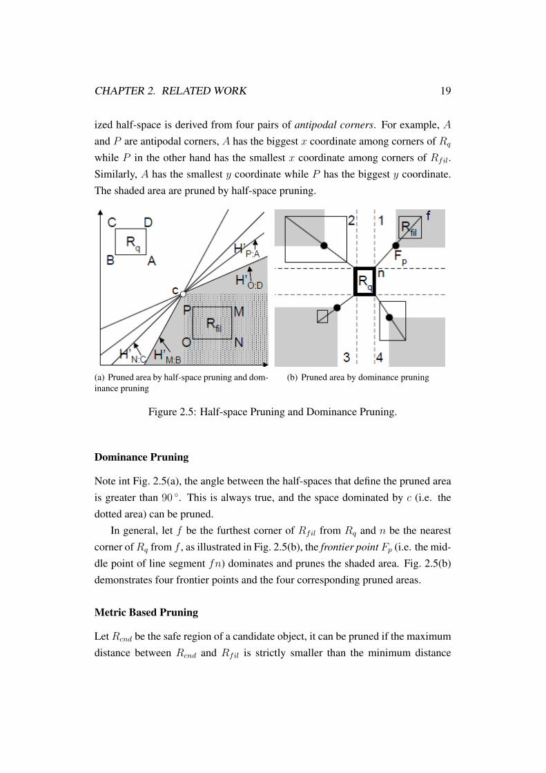
ized half-space is derived from four pairs of antipodal corners. For example, Aand P are antipodal corners, A has the biggest x coordinate among corners of Rq
while P in the other hand has the smallest x coordinate among corners of Rfil.Similarly, A has the smallest y coordinate while P has the biggest y coordinate.The shaded area are pruned by half-space pruning.
(a) Pruned area by half-space pruning and dom-inance pruning
(b) Pruned area by dominance pruning
Figure 2.5: Half-space Pruning and Dominance Pruning.
Dominance Pruning
Note int Fig. 2.5(a), the angle between the half-spaces that define the pruned areais greater than 90 ◦. This is always true, and the space dominated by c (i.e. thedotted area) can be pruned.
In general, let f be the furthest corner of Rfil from Rq and n be the nearestcorner of Rq from f , as illustrated in Fig. 2.5(b), the frontier point Fp (i.e. the mid-dle point of line segment fn) dominates and prunes the shaded area. Fig. 2.5(b)demonstrates four frontier points and the four corresponding pruned areas.
Metric Based Pruning
Let Rcnd be the safe region of a candidate object, it can be pruned if the maximumdistance between Rcnd and Rfil is strictly smaller than the minimum distance

CHAPTER 2. RELATED WORK 20
between Rcnd and Rq.
Pruning if Exact Location of Query is Known
As illustrated in Fig. 2.6, any point p that lies in the shaded area can be pruned,but p′, which is not in the shaded area, is the RNN of q if the filtering object isexactly at corner P .
Figure 2.6: Pruned area if exact location of query is known
2.3.2 Influence Zone
Cheema et. al introduce the novel concept influence zone in [6], which is the areasuch that every point inside it is RkNN of q and every point outside of it is notRkNN of q. This approach does not require a verification phase.
The main idea is using R-tree to index data points. Since data points that areclose to the query q are expected to prune larger area, data points and intermediateR-tree nodes are explored iteratively in increasing order of their minimum distanceto q.
Initially, the influence zone is the whole data space, and a min-heap h is ini-tialized with the root of the R-tree. If a de-heaped entry e completely lies outsideof all convex vertices of the current influence zone, it is ignored. Otherwise, its
CHAPTER 2. RELATED WORK 21
children are inserted in h if e is a R-tree node, or it is used to prune the space andupdate the influence zone if e is a data point.
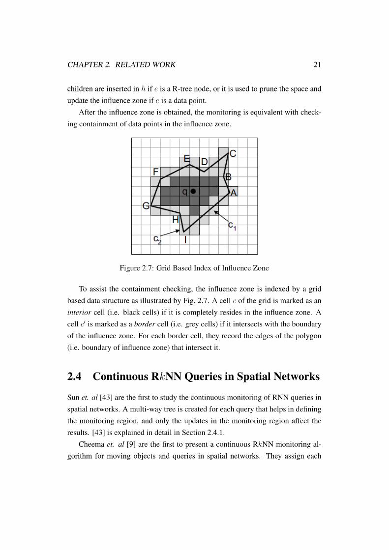
After the influence zone is obtained, the monitoring is equivalent with check-ing containment of data points in the influence zone.
Figure 2.7: Grid Based Index of Influence Zone
To assist the containment checking, the influence zone is indexed by a gridbased data structure as illustrated by Fig. 2.7. A cell c of the grid is marked as aninterior cell (i.e. black cells) if it is completely resides in the influence zone. Acell c′ is marked as a border cell (i.e. grey cells) if it intersects with the boundaryof the influence zone. For each border cell, they record the edges of the polygon(i.e. boundary of influence zone) that intersect it.
2.4 Continuous RkNN Queries in Spatial Networks
Sun et. al [43] are the first to study the continuous monitoring of RNN queries inspatial networks. A multi-way tree is created for each query that helps in definingthe monitoring region, and only the updates in the monitoring region affect theresults. [43] is explained in detail in Section 2.4.1.
Cheema et. al [9] are the first to present a continuous RkNN monitoring al-gorithm for moving objects and queries in spatial networks. They assign each
CHAPTER 2. RELATED WORK 22
moving object a safe region such that the pruning remains valid as long as the ob-jects remain in their respective safe regions. Although this avoids frequent calls tothe pruning phase, unfortunately the algorithm needs to verify a client wheneverit changes its location. The verification of a client is expensive because it requiresdetermining whether the query is one of the k closest facilities of the client ornot. We utilize the concept of influence zone to cheaply conduct the verification.Specifically, a client is confirmed as RkNN if and only if it is inside the influencezone. [9] is explained in detail in Section 2.4.2.
2.4.1 Multi-way Tree
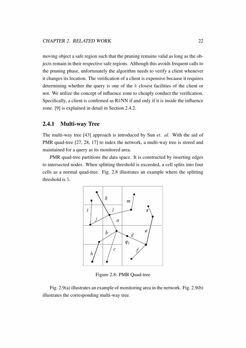
The multi-way tree [43] approach is introduced by Sun et. al. With the aid ofPMR quad-tree [27, 28, 17] to index the network, a multi-way tree is stored andmaintained for a query as its monitored area.
PMR quad-tree partitions the data space. It is constructed by inserting edgesto intersected nodes. When splitting threshold is exceeded, a cell splits into fourcells as a normal quad-tree. Fig. 2.8 illustrates an example where the splittingthreshold is 5.
Figure 2.8: PMR Quad-tree
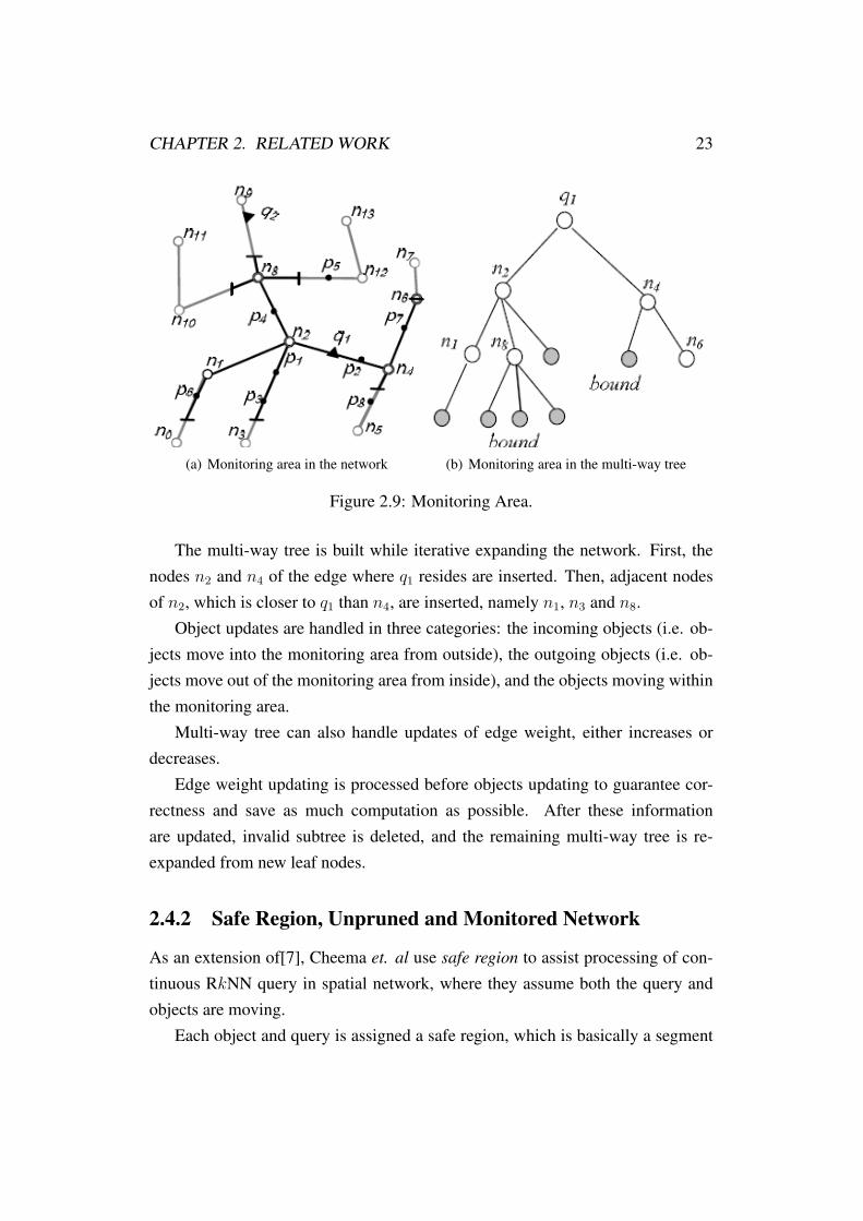
Fig. 2.9(a) illustrates an example of monitoring area in the network. Fig. 2.9(b)illustrates the corresponding multi-way tree.
CHAPTER 2. RELATED WORK 23
(a) Monitoring area in the network (b) Monitoring area in the multi-way tree
Figure 2.9: Monitoring Area.
The multi-way tree is built while iterative expanding the network. First, thenodes n2 and n4 of the edge where q1 resides are inserted. Then, adjacent nodesof n2, which is closer to q1 than n4, are inserted, namely n1, n3 and n8.
Object updates are handled in three categories: the incoming objects (i.e. ob-jects move into the monitoring area from outside), the outgoing objects (i.e. ob-jects move out of the monitoring area from inside), and the objects moving withinthe monitoring area.
Multi-way tree can also handle updates of edge weight, either increases ordecreases.
Edge weight updating is processed before objects updating to guarantee cor-rectness and save as much computation as possible. After these informationare updated, invalid subtree is deleted, and the remaining multi-way tree is re-expanded from new leaf nodes.
2.4.2 Safe Region, Unpruned and Monitored Network
As an extension of[7], Cheema et. al use safe region to assist processing of con-tinuous RkNN query in spatial network, where they assume both the query andobjects are moving.
Each object and query is assigned a safe region, which is basically a segment

CHAPTER 2. RELATED WORK 24
in the network, and could also be extended to contain more than one edges andsegments. Moreover, no two safe regions can intersect each other.
Each object and query reports its location to the server when it leaves its saferegion (i.e. source-initiated updates). In order to update results, the server mightneed to request the exact locations of some objects (i.e. server-initiated updates).
The proposed algorithm has two phases, listed as follows.
1. Filtering: The filtering phase is to retrieve a set of candidates. This isdone by pruning edges and segments of the network that cannot contain anyRkNN, and the remaining network, unpruned network, contains the set ofcandidates. The candidate set remains valid unless either the query or acandidate leaves its safe region or an object enters in the unpruned network.
2. Verification: With a valid unpruned network, the verification phase is in-voked at each timestamp. For Every candidate object, the query q is checkedof its eligibility to be a kNN.
Filtering Phase
The filtering phase is to incrementally expand the network in a way similar toDijkstra’s algorithm. The edges and segments that are explored during this processform the unpruned network. Six lemmas are used to prune unnecessary networks,listed as follows.
1. An object cannot be the RkNN if its shortest path to the query contains k
other objects.
2. An object cannot be the RkNN if its shortest path to the query q containsa dead vertex. A dead vertex v is a vertex such that there exist at least kother objects o have dist(v, o) < dist(v, q), where dist(a, b) is the networkdistance (i.e. shortest path) from a to b.
3. A vertex is a dead vertex if its shortest path to the query contains a deadvertex.

CHAPTER 2. RELATED WORK 25
4. For an edge (v1, v2) (v1 and v2 are the two end vertices of the edge) thatcontains at least 2k objects and does not contain the query q, the edge cannotcontain any RkNN if both dist(v1, q) and dist(v2, q) are longer than thelength of the edge.
5. Only the extreme objects of an edge (v1, v2) can be the RkNN of a query ifq does not resides on the edge. An extreme object o is an object such that atleast one of the two segments [o, v1] and [o, v2] contains at most k − 1 otherobjects.
6. Regardless of the number of queries in the system, an edge that does notcontain any query has at most 2k objects that can be the RkNNs of any ofthe queries.
Verification Phase
A straight forward but costly approach to verify a candidate is to issue a boolean
range query on the network with range set to the distance (i.e. network distance,the length of the shortest path between two points) from the candidate to the query.
One way to avoid boolean range query is by applying the forth lemma. If acandidate resides on an edge (v1, v2) such that the edge length is shorter than bothdist(v1, q) and dist(v2, q), a counter that records the number of objects on theedge is maintained. Objects are verified only when the counter shows that thereare at most k objects on the edge.
Another way to avoid time consuming boolean range query is based on theconcept of monitored network. Once the monitored network for an object is com-puted, the verification becomes computationally cheap. The monitored networkis computed during the filtering phase and remains valid as long as the unprunednetwork remains valid.
Monitored network of an object o is the part of the network such that for anypoint p that does not resides on it, minimum network distance from p to the saferegion of o is greater than maximum dist(o, q). Fig. 2.10 illustrates an exampleof monitored network of object o3.
Since for any object o′ that out of the monitored network of object o, the e-

CHAPTER 2. RELATED WORK 26
Figure 2.10: Monitored Network
quation dist(o, o′) > dist(o, q) holds, hence only objects resides in the monitorednetwork need to be considered at the time of verifying the eligibility of o to beRkNN of the query q.

Chapter 3
Overview
First, we present our motivation of this thesis in Section 3.1. Then, we formalizethe problem in Section 3.2. And last, we present an outline of our solution to theproblem in Section 3.3.
3.1 Motivation
Given a set of clients C and a set of facilities F , a client c ∈ C may find its near-by facilities by issuing a k nearest neighbors (kNN) query that returns k closestfacilities of c. Consider the example of a car driver who may issue a kNN queryto find his k closest gas stations and then may choose one of these gas stationsfor refueling. In contrast to a kNN query, a reverse k nearest neighbors (RkNN)query returns every client c ∈ C for which the query facility q ∈ F is one of thek closest facilities. Since q is close to such clients, q is said to have high influ-ence on these clients, i.e., q is likely to be used by such clients. Hence, the set ofsuch clients is also called influence set of q [22]. For instance, the owner of a gasstation may issue a RkNN query to find the cars for which his gas station is oneof the k closest gas stations. These car drivers are his potential customers and arelikely to be influenced by any promotional offer sent to them.
Throughout this thesis, we use RNN queries to refer to RkNN queries forwhich k = 1. The reverse k nearest neighbors (RkNN) query [22, 42, 52, 7, 6,4, 50, 19] has received significant attention ever since it was introduced in [22].
27
CHAPTER 3. OVERVIEW 28
RkNN queries have various applications such as decision support, location basedservices, resource allocation, profile-based management, etc. With the availabilityof inexpensive mobile devices, position locators and cheap wireless networks,location based services are gaining increasing popularity. An example of suchlocation based services is zhiing1. Consider that a user needs a taxi and she sendsher location to a taxi company’s dispatch center. The company notifies to a taxifor which she is the closest passenger (the taxi is a RNN of the user).
Other examples of location based services include location based games, traf-fic monitoring, location based SMS advertising, enhanced 911 services and armystrategic planning etc. These applications may require continuous monitoring ofreverse nearest moving clients. For instance, the owner of a gas station may wantto continuously monitor its RkNN cars and may decide to send them promotionaloffers from time to time. In this thesis, we study the problem of continuouslymonitoring RkNN queries in a road network where the clients (e.g., cars) are con-tinuously moving and the facilities (e.g., gas stations) are static.
The existing best known solution (Lazy Updates [9]) monitors the RkNNqueries in two major steps. In pruning phase, pruning rules are used to prunethe part of the road network such that any client in the pruned region cannot bethe RkNN of the query. The clients that are in the unpruned network are called thecandidate objects. In monitoring phase, the server conducts verification for eachcandidate object c to verify whether it is a RkNN or not. Specifically, a candidateobject c is reported as a RkNN if and only if q is one of its k closest facilities.At each time stamp (e.g., after every t time units), the server needs to conduct theverification for the clients that are inside the unpruned network and have changedtheir locations during the last time stamp. This is quite expensive because i) ver-ifying a candidate c requires checking whether q is one of the k closest facilitiesof c or not and ii) the verification is required as soon as a candidate changes itslocation.
To address the above limitation, we use the novel concept of influence zone
that we introduced in [6, 8] for answering RkNN queries in Euclidean space. Theinfluence zone Zk of a query q is the region such that q is one of the k closestfacilities of a client c if and only if c is inside this region, i.e., c is a RkNN if and
1http://www.zhiing.com/how.php
CHAPTER 3. OVERVIEW 29
only if c is inside the influence zone. Our solution also has two major steps. Inthe first phase, we compute the influence zone Zk of the query. Once the influencezone is computed, it is straightforward to monitor the RkNNs of query by moni-toring the clients that are inside the influence zone. Hence, in the second phase,we report every client that lies inside the influence zone. At each time stamp, theclients that move inside the influence zone are reported as new RkNNs and theclients that move out of the influence zone are removed from the answer. Thissignificantly reduces the computation cost because we only need to monitor theclients that enter or leave the influence zone. Our extensive experimental evalua-tion demonstrates that our influence zone based approach is more than an order ofmagnitude better than the state-of-the-art algorithm [9].
Although the focus of this thesis is on continuous RkNN queries, we remarkthat the influence zone has applications also in marketing and decision supportsystems. Consider the example of a restaurant. Its influence zone may be used asmarket analysis as well as targeted marketing. For instance, the demographics ofits influence zone may be used by the market researchers to analyse its business.The influence zone can also be used for marketing, e.g., advertising bill boardsor posters may be placed in its influence zone because the people in this areaare more likely to be influenced by the marketing. Similarly, the people in itsinfluence zone may be sent SMS advertisement.
In our previous work [6, 8], we presented efficient algorithm to compute in-fluence zone in Euclidean space. In this thesis, we address the applications thatuse road network distance as underlying distance metric and propose efficien-t techniques to compute the influence zone in road networks. Unfortunately, theexisting algorithms for Euclidean space cannot be applied or extended for roadnetworks due to inherently different characteristics of Euclidean space and roadnetworks.
3.2 Problem Formulation
Reverse k nearest neighbors (RkNN) query: Given a set of points C represent-ing client objects, a set of points F representing facility objects, and a query pointq ∈ F , a RkNN query retrieves every point c ∈ C such that q is one of the k

CHAPTER 3. OVERVIEW 30
closest facilities of c. In this thesis, we focus on RkNN queries considering theroad network distance.
Example 1 Consider the example of Fig. 3.1 that includes three facilities (shown
as square) f1, f2 and q on a road network along with three clients (shown as
triangles) c1, c2 and c3. c1 is the RNN (k = 1) of the query q because q is its
closest facility. On the other hand, c2 and c3 are not its RNN because the closest
facility for both c2 and c3 is f2. Similarly, R2NNs (k = 2) of the query q include
the clients c1 and c3. The client c2 is not the R2NN because q is not one of its 2
closest facilities.
Figure 3.1: Illustration of RkNN queries
Snapshot RkNN Queries vs Continuous RkNN Queries: In a snapshot RkNNquery, the results are to be computed only once. On the other hand, in a con-tinuous RkNN query the results of the query are to be continuously monitoredas the location of underlying data objects (e.g., clients and/or facilities) change.In this thesis, we focus on continuous monitoring of RkNN queries. Like manyreal world scenarios, we assume that the clients (e.g., cars, pedestrians etc.) aremoving whereas the facilities (e.g., gas stations, restaurants etc.) are static. Ateach time stamp (i.e., after every t time units), the server receives a set of updatesthat contains the new locations of the clients that have moved during the last timestamp. Upon receiving these location updates, the server updates the results of theRkNN queries accordingly.
CHAPTER 3. OVERVIEW 31
3.3 Solution Overview
The key idea is to compute the influence zone for the query. The influence zone ofa query q is a part of the network such that every client c that lies inside the zone isthe RkNN of q and every client c that lies outside the zone is not its RkNN. Oncethe influence zone is computed, the problem is reduced to monitoring the clientsthat are inside the influence zone. We give a formal definition of the influencezone below.
Definition 3.3.1 Given a spatial network G, a set of facilities F = {f1, f2, · · · , fn}where fi denotes the location of the ith facility on G, and a query facility q ∈ F ,
the influence zone Zk is a sub network (Zk ⊆ G) such that for every point p ∈ Zk,
q is one of the k closest facilities of p, and for every point p′ /∈ Zk, q is not one of
the k closest facilities of p′.
Example 2 In Fig. 3.2(a), the influence zone Z1 (i.e., k = 1) is the part of the
network shown using thick lines. Note that any point (e.g., c1) that lies in the
influence zone is the RNN of q whereas any point (e.g., c2 and c3) that do not lie
on the influence zone are not the RNNs of q. Fig. 3.2(b) illustrates the influence
zone Z2 (e.g., k = 2) using the thick lines. Since c1 and c3 lie inside the influence
zone, these two clients are the R2NNs of q. On the other hand, c2 is not the R2NN
of q because it lies outside the influence zone.
Note that the influence zone does not change as long as the locations of thefacilities do not change. As stated earlier, in our problem settings, the facilities(e.g., gas stations) do not change their locations. Therefore, once the influencezone has been computed, it is not required to be updated.
Based on the concept of the influence zone, we develop our continuous RkNNmonitoring algorithm. It consists of two phases namely influence zone calculation
phase (Chapter 4) and monitoring phase (Section 4.6). As is obvious from thename, in the influence zone calculation phase, the influence zone of the query iscomputed. Since a client is the RkNN of q if and only if it is inside the influencezone, once the influence zone has been computed, we only need to monitor theclients that lie inside the influence zone. In the monitoring phase, the algorithm

CHAPTER 3. OVERVIEW 32
(a) influence zone Z1 (k = 1) (b) influence zone Z2 (k = 2)
Figure 3.2: A simple spatial network example.
monitors the clients that are inside the influence zone. More specifically, whenevera client moves, the server checks whether it lies inside the influence zone or not.If it is inside the influence zone, it is reported as the RkNN.
In the next Chapter, we present techniques to efficiently calculate the influencezone. In Section 4.6, we demonstrate efficient techniques to determine whether aclient lies inside the influence zone or not.
Chapter 4
Influence Zone Based Techniques
For the ease of presentation, we treat the query point q as a node. For example,in Fig. 4.1, we assume that q is a node and n1 and n3 are its adjacent nodes inthe network. Note that this assumption is made only for the simplification of thepresentation and is not a requirement for our algorithm to work correctly.
Before we present our solution, we first define some terms and notations inSection 4.1. We present problem characteristics in Section 4.2 followed by ourtechniques in Section 4.3 and Section 4.4. We present the extension of our tech-niques to directed graph in Section 4.5. We explain how to use the influence zoneto efficiently monitor RkNN query in Section 4.6.
4.1 Terms and Notations
Table 4.1 defines the terms and notations used throughout this thesis.Inner Node: A node that resides in the influence zone is called an inner node.
Table 4.1: NotationsSymbol DescriptionG spatial networkni ith nodeE(n1, n2) An edge between nodes n1 and n2
Zk influence zoneDist(p1, p2) length of the shortest path between p1 and p2S[p1, p2] the part of an edge between p1 and p2
33

CHAPTER 4. INFLUENCE ZONE BASED TECHNIQUES 34
Outer Node: A node that resides outside of the influence zone is called an outer
node.Bounding Node: An outer node is called a bounding node if at least one of itsadjacent nodes is an inner node.
Example 3 In Fig. 3.2(a) (k = 1), n1 is an inner node because it lies in the
influence zone. On the other hand, n2, n3 and n4 are the outer nodes. Since n1
is an inner node and is an adjacent node of n2, n2 is a bounding node. Similarly,
n3 is also a bounding node whereas n4 is not a bounding node. In the example of
Fig. 3.2(b) (k = 2), n1, n2 and n3 are inner nodes whereas n4 is an outer node as
well as a bounding node.
Inner Edge: An edge that completely lies inside the influence zone is called aninner edge, i.e., an edge E(n1, n2) is an inner edge if, for every point p ∈ E,p ∈ Zk.Outer Edge: An edge that completely lies outside the influence zone is calledan outer edge, i.e., an edge E(n1, n2) is an outer edge if, for every point p ∈ E,p /∈ Zk.Partial Edge: An edge that only partially lies inside the influence zone is calleda partial edge, i.e., an edge E(n1, n2) is a partial edge if there exists p ∈ E suchthat p ∈ Zk and there exists p′ ∈ E such that p′ /∈ Zk.Inner Segment: An inner segment is the part of a partial edge that lies in theinfluence zone. A segment between two points p1 and p2 is denoted as S[p1, p2].
Example 4 In Fig. 3.2(a), the edge E(n1, n2) is a partial edge and the edge
E(n3, n4)is an outer edge. In Fig. 3.2(b), the edge E(n1, n2) is an inner edge
whereas the edge E(n3, n4) is a partial edge. In Fig. 3.2(b), the segment S[n3, f2]
is an inner segment.
Note that an influence zone can be described by a set of inner nodes, a set ofinner edges and a set of inner segments.
4.2 Properties
In this section, we present two properties that support our basic algorithm.

CHAPTER 4. INFLUENCE ZONE BASED TECHNIQUES 35
Lemma 4.2.1 A node n is an inner node iff the k closest facilities of n include q.
The proof is straightforward hence omitted.
Lemma 4.2.2 An edge E(n1, n2) is an outer edge if both n1 and n2 are the outer
nodes1.
Proof We prove this by contradiction. Assume a point p ∈ E that lies insid-e the influence zone, i.e., the k closest facilities of p include q. Without loseof generality, assume that the shortest path from p to q goes through the noden1, i.e., Dist(p, q) = Dist(p, n1) + Dist(n1, q). Consider a facility f such thatDist(n1, f) < Dist(n1, q). For such facility f , Dist(p, f) ≤ Dist(p, n1) +
Dist(n1, f). Since Dist(n1, f) < Dist(n1, q), Dist(p, f) < (Dist(p, n1) +
Dist(n1, q) = Dist(p, q)). In other words, f is closer to p than q. Since n1 isan outer node, there are at least k such facilities and this implies that there are atleast k facilities closer to p than q. Hence, p does not lie inside the influence zonewhich is a contradiction to our assumption.
Example 5 In Fig. 3.2(a), both n2 and n3 are the outer nodes and the edge
E(n2, n3) is an outer edge.
Remark 1 A reader may incorrectly assume that an edge E(n1, n2) is always an
inner edge if both n1 and n2 are the inner nodes. However, this is not true. For
instance, in Fig. 3.2(b), n2 and n3 both are inner nodes but E(n2, n3) is not an
inner edge (it is a partial edge).
As aforementioned, influence zone consists of inner edges and inner segments.Therefore, to calculate influence zone, all the inner edges and inner segments mustbe identified. According to Lemma 4.2.2, an edge between two outer nodes isalways an outer edge. Hence, to compute the inner edges and inner segments, weonly need to identify inner nodes and bounding nodes (Section 4.3). Based on theinner and bounding nodes, we can then determine the inner edges and the innersegments (Section 4.4).
1Recall that, for the ease of presentation, we treat the query point q as a node in the network.Hence, if a query q lies on an edge E(n1, n2), the edge is considered to be divided into two edgesE(n1, q) and E(q, n2) and the lemma is applied on both of the edges.

CHAPTER 4. INFLUENCE ZONE BASED TECHNIQUES 36
4.3 Identifying Inner Nodes and Bounding Nodes
A naıve approach to identify inner nodes is to apply Lemma 4.2.1 for all the nodesin the spatial network. However, this is quite expensive because the lemma is tobe applied for every node in the network. Next, we present a lemma which allowsus to identify all the inner nodes by applying Lemma 4.2.1 only on the inner nodesand the bounding nodes.
Lemma 4.3.1 A node n is an outer node if the shortest path from n to q goes
through another outer node n′.
Proof As the shortest path from n to q goes through n′, Dist(n, q) = Dist(n, n′)+
Dist(n′, q). Since n′ is an outer node, we know that there are at least k facil-ities such that for each such facility f , Dist(n′, f) < Dist(n′, q). For each ofthese k facilities f , Dist(n, f) ≤ Dist(n, n′) +Dist(n′, f). Since Dist(n′, f) <
Dist(n′, q), Dist(n, f) < (Dist(n, n′) +Dist(n′, q) = Dist(n, q)). Thus, eachof these k facilities f satisfies Dist(n, f) < Dist(n, q). Hence q is not one of thek closest facilities of n, i.e., n is an outer node.
We remark that, in the case where there are multiple shortest paths from n toq, Lemma 4.3.1 holds as long as at least one of these shortest paths goes throughan outer node.
Example 6 In Fig. 3.2(a), n3 is an outer node. The shortest path from n4 to q
goes through n3. Therefore, n4 is also an outer node (as can be verified because
f2 is also closer to n4 than q).
We explore the network starting from q using network expansion similar toDijkstra’s algorithm. As per Lemma 4.3.1, as soon as an outer node is encoun-tered, further expansion from this node is not required. Algorithm 1 presents thedetails.
Algorithm 1 explores the network starting from q in an iterative expansionmanner. Line 1 initializes a min heap h by inserting q with key set to zero. Recallthat we treat q as a node in the network. The key of each node n in the heapis its network distance to q. For each de-heaped node n, we mark n as an inner

CHAPTER 4. INFLUENCE ZONE BASED TECHNIQUES 37
Algorithm 1 Inner Nodes and Bounding NodesInput: G, a set of facilities F , a query point q ∈ F , kOutput: a set of inner nodes, a set of bounding nodes
1: insert q in a min-heap h2: while h is not empty do3: deheap an node n, mark n as visited4: if k closest facilities of n include q then5: mark n as inner node and mark it visited6: for each unvisited adjacent node n′ of n do7: if n′ not in h then8: insert n′ in h9: else if a shorter path from n′ to q found then
10: update n′ in h11: else12: mark n as bounding node and mark it visited
node if q is one of its k closest facilities (lines 4 and 5). Furthermore, for eachadjacent node n′ of n, the algorithm inserts (or updates) n′ in h along with itsminimum network distance to q (lines 6 to 10). On the other hand, n is marked asa bounding node if q is not one of the k closest facilities of n (line 12). Accordingto Lemma 4.3.1, the network is not required to be expanded beyond any outer (orbounding) node. Therefore, the adjacent nodes of n are not inserted in h in thiscase. The algorithm terminates when the heap becomes empty. It can be easilyverified that the algorithm identifies (and marks) all the inner and bounding nodesbefore it terminates.
A straightforward way to check if the k closest facilities of n include q (line 4)is to explore the network starting from the node n with a search area bounded byDist(n, q) and counting the number of facilities encountered during the search.We remark that a more efficient approach is to utilize the Euclidean distance boundto quickly conduct this check in some cases. More specifically, a Euclidean spacecircular range query [5] centered at n with range set as Dist(n, q) can be issued.If the Euclidean range query returns less than k facilities, it guarantees that q isone of the k closest facilities of n in terms of network distance. This is becauseEuclidean distance serves as a lower bound network distance and if there are lessthan k facilities with Euclidean distance from n smaller than Dist(n, q) then there

CHAPTER 4. INFLUENCE ZONE BASED TECHNIQUES 38
are less than k facilities closer to n than q in terms of network distance. Euclideanrange query can be efficiently conducted using an index structure such as R-treeif available.
4.4 Calculating Inner Edges and Inner Segments
In this section, we demonstrate how to compute inner edges and inner segmentsonce the inner and bounding nodes have been identified using Algorithm 1. Tofacilitate the presentation, we first introduce the concept of monotonic edges.Monotonic Edge: An edge E(n1, n2) is called a monotonic edge if the shortestpath from n2 to q goes through n1 or the shortest path from n1 to q goes throughn2. A monotonic edge E(n1, n2) is denoted as Em(n2, n1) if the shortest pathfrom n2 to q goes through n1, and it is denoted as Em(n1, n2) if the shortest pathfrom n1 to q goes through n2.
Figure 4.1: Influence zone Z1 (k = 1)
Non-monotonic Edge: Any edge that is not a monotonic edge is called a non-monotonic edge and is denoted as En(n1, n2).
Example 7 Fig. 4.1 shows two monotonic edges Em(n2, n1) and Em(n4, n3).
En(n2, n3) and En(n2, n4) are non-monotonic edges.
Next, we present techniques on how to compute inner edge and inner segmentfor a monotonic edge. Later in Section 4.4.2, we show that a non-monotonic edge

CHAPTER 4. INFLUENCE ZONE BASED TECHNIQUES 39
can be easily broken into two monotonic edges and the techniques for monotonicedges can then be applied on each of the two monotonic edges.
4.4.1 Handling Monotonic Edges
Before we present our techniques, we present a few terms and two properties ofmonotonic edges.Pruner: A facility f is said to prune a point p if Dist(p, f) < Dist(p, q) and f
is called a pruner of p. Note that a point p is the RkNN of a query q if and onlyif there exist less than k pruners of p. In other words, a point p that has less thank pruners lies in the influence zone, and a point p′ that has at least k pruners liesoutside the influence zone.
Example 8 Consider the example of Fig. 4.1, f is a pruner of n3. Furthermore,
n3 is not a RNN of q because it has one pruner.
Lemma 4.4.1 Given a monotonic edge Em(n2, n1), a facility f that prunes n1
also prunes every point p ∈ Em(n2, n1).
Proof Assume that there is a point p ∈ Em(n2, n1) such that f is not a prunerof p, i.e., Dist(p, f) ≥ Dist(p, q). Since f is a pruner of n1, we know thatDist(n1, f) < Dist(n1, q). Furthermore, since Em(n2, n1) is a monotonic edge,the shortest path from p to q goes through n1. This means Dist(p, q) = Dist(p, n1)+
Dist(n1, q). Since Dist(n1, f) < Dist(n1, q), Dist(p, q) > (Dist(p, n1) +
Dist(n1, f) ≥ Dist(p, f)). This contradicts the assumption that Dist(p, f) ≥Dist(p, q).
Example 9 Consider the monotonic edge Em(n4, n3) in Fig. 4.1, f is a pruner of
n3 and it can be verified that f is also a pruner of every point on Em(n4, n3).
Lemma 4.4.2 Given a monotonic edge Em(n2, n1), a facility f that does not
prune n2 cannot prune any point p ∈ Em(n2, n1).
Proof Assume that f does not prune n2 but prunes a point p ∈ Em(n2, n1), i.e.,Dist(p, f) < Dist(p, q). Since Em(n2, n1) is a monotonic edge, Dist(n2, q) ≥

CHAPTER 4. INFLUENCE ZONE BASED TECHNIQUES 40
Dist(n2, n1). Since f does not prune n2 (i.e., Dist(n2, f) ≥ Dist(n2, q)), it isimmediate that Dist(n2, f) ≥ Dist(n2, n1). This implies that if f lies on the edgeE, it lies at the node n1 otherwise it lies outside the edge. Hence, the shortest pathfrom p to f must go through either n1 or n2.
If the shortest path from p to f goes through n1 then Dist(p, f) ≥ Dist(n2, f)−Dist(n2, p). This is because Dist(n2, f) ≤ Dist(n2, p) + Dist(p, f). On theother hand, if the shortest path from p to f goes through n2 then Dist(p, f) =
Dist(p, n2) + Dist(n2, f). Therefore, in any case, Dist(p, f) ≥ Dist(n2, f) −Dist(n2, p). Since Dist(n2, f) ≥ Dist(n2, q) (because f does not prune n2),Dist(p, f) ≥ Dist(n2, q) −Dist(n2, p). Since Em(n2, n1) is a monotonic edge,Dist(p, q) = Dist(n2, q) − Dist(n2, p). Hence, Dist(p, f) ≥ Dist(p, q) whichcontradicts the assumption.
Example 10 Consider the example of the monotonic edge Em(n2, n1) in Fig. 4.1.
Since f does not prune n2, it can be verified that f does not prune any point on
Em(n2, n1).
Based on the above lemmas, next we show how to compute inner edge andinner segment for a monotonic edge.Identifying inner edge. Recall that an inner edge is an edge that completelyresides in the influence zone. The next lemma shows that a monotonic edge is aninner edge if and only if its nodes are inner nodes.
Lemma 4.4.3 A monotonic edge Em(n2, n1) is an inner edge iff both n1 and n2
are inner nodes.
Proof Assume that both n1 and n2 are inner nodes. Since n2 is an inner node,there are less than k facilities that prune n2, i.e., at least |F | − k facilities cannotprune n2 where |F | is the total number of facilities. According to Lemma 4.4.2, afacility f that does not prune n2 cannot prune any point p ∈ Em(n2, n1). Hence,there are at least |F | − k facilities that do not prune any point p ∈ Em(n2, n1).Hence, every such point p is inside the influence zone which implies that the edgeis an inner edge.
If at least one of n1 or n2 is not an inner node, then the edge is not an inneredge (it is a partial edge because at least one point is outside the influence zone).

CHAPTER 4. INFLUENCE ZONE BASED TECHNIQUES 41
Lemma 4.4.3 can be applied to identify whether a monotonic edge is an inneredge or not. Next, we show how to compute the inner segment of a monotonicedge if the edge is not an inner edge (i.e., is a partial edge).Identifying inner segments. Recall that an inner segment is the part of a partialedge that lies in the influence zone. For instance, in Fig. 4.2, S[n1, p1] is an innersegment. Below, we show how to identify inner segments.
Figure 4.2: Influence zone Z2 (k = 2)
Given an edge Em(n2, n1), for each facility f that prunes at least one pointof this edge, we first identify the segment of the edge that is pruned by f . Asimplied by Lemma 4.4.2, a facility f that prunes at least one point of a monotonicedge Em(n2, n1) must always prune n2. Therefore, for each facility, the prunedsegment always includes n2, i.e., the pruned segment is S[p, n2] where p is a pointon the edge. Once we identify all segments that are pruned by the facilities, theinner segment of the edge corresponds to the part of the edge that is pruned byless than k facilities. The example below illustrates this.
Example 11 Fig. 4.3 illustrates how to compute the inner segment of Em(n2, n1)
for the example of Fig. 4.2. For each of the facilities f1, f2 and f3, it demonstrates
the segment (shown thick) pruned by the corresponding facility. For instance, f1prunes the whole edge whereas f2 prunes the part of the edge between p1 and n2.
Note that the segment S[n1, p1] is pruned by less than 2 facilities so it lies inside

CHAPTER 4. INFLUENCE ZONE BASED TECHNIQUES 42
Figure 4.3: Inner segment is the segment pruned by less than k facilities.
the influence zone and is the inner segment (considering k = 2). Note that such
point p1 can be easily identified given the pruned segments for each facility.
Next, we show how to identify the segment of a monotonic edge Em(n2, n1)
pruned by a facility f . The facility prunes the whole edge if it prunes n1 (Lem-ma 4.4.1) and it does not prune any point of the edge if it does not prune n2
(Lemma 4.4.2). For the case when f prunes n2 but does not prune n1, it prunes asegment S[p, n2] of the edge where p is a point on the edge that lies at a distanced from n2 and d is calculated by Equation (4.1).
d =
{Dist(n2,q)+Dist(n2,f)
2if f is on Em(n2, n1)
Dist(n2,q)−Dist(n2,f)2
if f is not on Em(n2, n1)(4.1)
The proof is omitted for brevity, however, it can be verified easily.
Example 12 In Fig. 4.2, the segment pruned by f2 is S[p1, n2] where p1 is a point
with distance d = 12(Dist(n2, q) + Dist(n2, f2)) = 1
2(8 + 2) = 5 from n2.
The segment pruned by f3 is S[p2, n2] where p2 is a point with distance d =12(Dist(n2, q)−Dist(n2, f3)) =
12(8− 6) = 1 from n2.
A final issue to be addressed with the above approach is that it requires com-puting the pruned segment for every facility f regardless of whether it prunes apart of the edge or not. This can be easily addressed as follows. As per Lem-ma 4.4.2, if a facility f does not prune n2, it cannot prune any part of the edge.Hence, the pruned segment is required to be computed only for the facilities that

CHAPTER 4. INFLUENCE ZONE BASED TECHNIQUES 43
prune n2. Therefore, we retrieve and store the facilities that prune n2 when wecheck whether n2 is an inner node or not (at line 4 of Algorithm 1). These facili-ties are then used to determine the inner segment as described above.
4.4.2 Handling Non-monotonic Edges
We handle a non-monotonic edge En(n1, n2) by introducing an imaginary node xon this edge that divides it into two monotonic edges Em(x, n1) and Em(x, n2).Then, the techniques presented in previous section can be applied on each of thesemonotonic edges to compute the corresponding inner segments.
Figure 4.4: Handling non-monotonic edge.
Example 13 Fig. 4.4 illustrates an example of a non-monotonic edge En(n1, n2).
Dist(n1, q) = 6 and Dist(n2, q) = 7. It also demonstrates a point x on the edge
such that Em(x, n1) is a monotonic edge , i.e., the shortest path from x to q goes
through n1. Similarly, Em(x, n2) is also a monotonic edge.
The point x is a point such that the length of its shortest path to q passingthrough n1 is the same as the length of its shortest path to q passing through n2
(i.e., Dist(x, q) = Dist(x, n1)+Dist(n1, q) = Dist(x, n2)+Dist(n2, q)). Note,Dist(x, q) = 1
2(Dist(n1, n2) +Dist(n1, q) +Dist(n2, q)). It can be verified that
the point x is a point that lies at distance d from n2 where d is calculated asfollows:
CHAPTER 4. INFLUENCE ZONE BASED TECHNIQUES 44
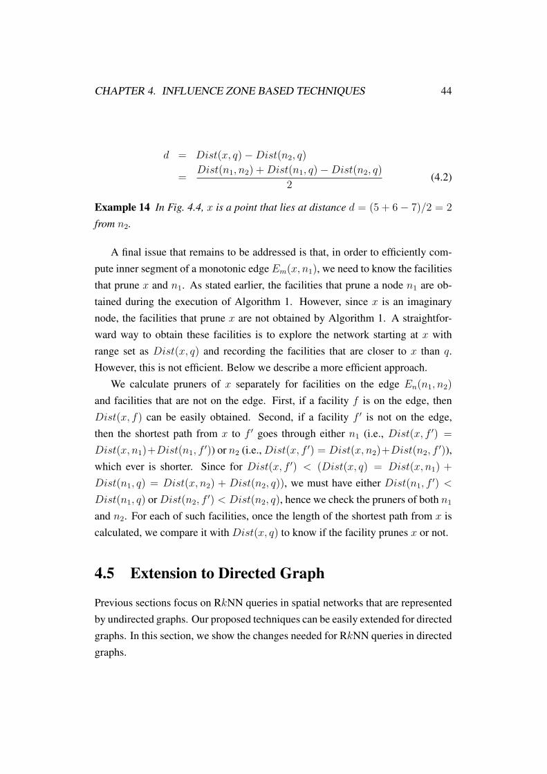
d = Dist(x, q)−Dist(n2, q)
=Dist(n1, n2) +Dist(n1, q)−Dist(n2, q)
2(4.2)
Example 14 In Fig. 4.4, x is a point that lies at distance d = (5 + 6− 7)/2 = 2
from n2.
A final issue that remains to be addressed is that, in order to efficiently com-pute inner segment of a monotonic edge Em(x, n1), we need to know the facilitiesthat prune x and n1. As stated earlier, the facilities that prune a node n1 are ob-tained during the execution of Algorithm 1. However, since x is an imaginarynode, the facilities that prune x are not obtained by Algorithm 1. A straightfor-ward way to obtain these facilities is to explore the network starting at x withrange set as Dist(x, q) and recording the facilities that are closer to x than q.However, this is not efficient. Below we describe a more efficient approach.
We calculate pruners of x separately for facilities on the edge En(n1, n2)
and facilities that are not on the edge. First, if a facility f is on the edge, thenDist(x, f) can be easily obtained. Second, if a facility f ′ is not on the edge,then the shortest path from x to f ′ goes through either n1 (i.e., Dist(x, f ′) =
Dist(x, n1)+Dist(n1, f′)) or n2 (i.e., Dist(x, f ′) = Dist(x, n2)+Dist(n2, f
′)),which ever is shorter. Since for Dist(x, f ′) < (Dist(x, q) = Dist(x, n1) +
Dist(n1, q) = Dist(x, n2) + Dist(n2, q)), we must have either Dist(n1, f′) <
Dist(n1, q) or Dist(n2, f′) < Dist(n2, q), hence we check the pruners of both n1
and n2. For each of such facilities, once the length of the shortest path from x iscalculated, we compare it with Dist(x, q) to know if the facility prunes x or not.
4.5 Extension to Directed Graph
Previous sections focus on RkNN queries in spatial networks that are representedby undirected graphs. Our proposed techniques can be easily extended for directedgraphs. In this section, we show the changes needed for RkNN queries in directedgraphs.

CHAPTER 4. INFLUENCE ZONE BASED TECHNIQUES 45
Since it can be verified that lemmas 4.2.1, 4.2.2 and 4.3.1 still hold, Algorith-m 1 can be used in a similar way. The only difference is that for unidirectionaledges the expansion follows only the reverse direction (i.e., at line 6 of Algorith-m 1, a node n′ is considered the adjacent node of n if and only if the edge is eitherbidirectional or the direction of the edge is from n′ to n).
Lemmas 4.4.1, 4.4.2 and 4.4.3 hold for bidirectional edges. Once inner andbounding nodes are identified, bidirectional edges can be handled the same as inan undirected graph. Although these lemmas are not applicable for unidirectionaledges, this issue can be easily addressed as below.
Let Eu(n1, n2) be an unidirectional edge goes from n1 to n2. The shortest pathfrom n1 to a facility f or q may not go through n2. Apart from n1, the shortestpath from every other point p ∈ Eu(n1, n2) to a facility f /∈ S[p, n2] or q must gothrough n2. This means, on one hand, a facility f ∈ Eu(n1, n2) prunes a segmentS[n1, f ] (note, n1 is excluded), and on the other hand, a facility f ′ /∈ Eu(n1, n2)
such that Dist(n2, f′) < Dist(n2, q) prunes every point p ∈ Eu(n1, n2) (note,
n1 is included). Recall that the inner segment can be easily identified given thepruned segments for each facility.
(a) influence zone Z1 (k = 1) (b) influence zone Z2 (k = 2)
Figure 4.5: A simple directed spatial network example.
Example 15 Fig. 4.5 gives a simple example on directed spatial network. Direc-
tion of edges are marked by arrows. For example, bidirectional edge E(n1, n3)

CHAPTER 4. INFLUENCE ZONE BASED TECHNIQUES 46
has arrows at both ends, and unidirectional edge Eu(n2, n1) has arrow pointing
at n1, which means it goes from n2 to n1.
Since n1 has no pruner, Eu(n2, n1) (n2 excluded) has no pruner. f1 ∈ Eu(n2, n4)
prunes S[n2, f1], and since n2 is pruned by f1, Eu(n3, n2) (n3 excluded) is pruned
as well. Similarly, f2 ∈ Eu(n4, n3) prunes S[n4, f2], and also prunes the whole
edge Eu(n2, n4). Fig. 4.5(a) shows the influence zone when k = 1, and Fig. 4.5(b)
shows the influence zone when k = 2.
4.6 Monitoring Phase
Once the influence zone is computed, we only need to monitor the clients that liein the influence zone. In real world applications, there may be multiple RkNNqueries issued by different users. In this section, we show how to efficiently mon-itor the results of all RkNN queries.
Figure 4.6: Index of influence zones.
For each edge E of the network, we maintain two lists. The first list callededge list contains query ID of every query q for which E is an inner edge. Thesecond list called segment list contains query ID of every q for which E containsan inner segment (the inner segment is also stored as shown in Fig. 4.6).
Whenever a client moves from a location locold to locnew, we update the resultsof the affected queries as follows. Without loss of generality assume that locold(resp. locnew) lies on an edge Eold (resp. Enew). Note that the results of everyquery q are changed if the client leaves or enters its influence zone. Note that ifa client leaves (resp. enters) an influence zone, its locold (resp. locnew) must beinside its influence zone. Hence, we look in the edge list and segment list of Eold
and identify every query q for which the client c was in its influence zone, i.e., qis present in the edge list of Eold or q is present in the segment list of Eold and c
lies in the inner segment. For each such query q, the client c is removed from its

CHAPTER 4. INFLUENCE ZONE BASED TECHNIQUES 47
RkNN. Then, we look in the edge list and inner segment list of Enew and identifythe queries for which c is now in its influence zone. For each such query q, c isadded as a RkNN.

Chapter 5
Experiments
In this section, we evaluate the performance of our algorithm for RkNN queries.We first illustrate the size of influence zone in section 5.2, and then evaluate thetotal running time of our approach in section 5.3, and finally we evaluate thecomputation cost of the influence zone calculation phase in section 5.4.
5.1 Experimental Settings
All the experiments were conducted on Intel Xeon 2.4 GHz dual CPU with 4GBytes memory. All the algorithms (including the competitors) were implement-ed in C++. Our algorithm is named IZone. We compare our algorithm with thestate-of-the-art algorithm for RkNN monitoring in spatial networks, Lazy Updateswhich is also known as SAC [9].
We use the road network of California that consists of 21048 nodes, 21693edges and 87635 points of interest. For the experiment where we vary the numberof facilities, we randomly select facilities from the 87635 points of interest. Themoving clients follow a random moving path, e.g., a client moves on an edge witha given speed and when it reaches the end node, it randomly selects a neighboringedge and continues moving on it.
Table 5.1 shows the system parameters used in our experiments, default valuesare shown in bold. The server reports the results continuously at each time stamp.We assume that the time stamp length is 1 second. All queries are continuously
48

CHAPTER 5. EXPERIMENTS 49
Table 5.1: System Parameters for ExperimentsParameter RangeNumber of clients (×1000) 50, 75, 100, 125, 150Percentage of clients moving 20, 40, 60, 80, 100Speed of clients (km/h) 60, 70, 80, 90, 100, 110, 120Number of queries 1, 10, 100, 1000Number of facilities (×1000) 2, 4, 8, 16, 32, 64k 1, 2, 4, 8, 16, 32, 64
monitored for 5 minutes (e.g., 300 time stamps) and the results correspond to thetotal running time of all queries monitored for the 5 minutes duration.
5.2 Influence Zone Size
In this section, we illustrate how the size of influence zone is affected by differentsystem parameters. The size of the influence zone is important because the totalrunning cost is directly proportional to the size of the influence zone (e.g., thelarger the influence zone is, the greater the number of RkNNs of q is). The size ofthe influence zone is the total length of all the inner edges and inner segments.
0
50
100
150
200
250
300
2 4 8 16 32 64
Net
wor
k Le
ngth
(in
km
)
Number of facilities (in 1,000)
(a) Effect of number of facilities
0
50
100
150
200
250
300
350
1 2 4 8 16 32 64
Net
wor
k Le
ngth
(in
km
)
k
(b) Effect of k
Figure 5.1: Influence zone size.
Fig. 5.1(a) shows the effect of the number of facilities on the size of influencezone. The influence zone becomes smaller when the number of facilities increas-es. This is because the distance from a client to its k closest facilities is inverselyproportional to the number of facilities.

CHAPTER 5. EXPERIMENTS 50
Fig. 5.1(b) shows the effect of k on the size of influence zone. As expected,the size of influence zone increases with the value of k. This is because, for alarger value of k, a client is influenced by facilities located farther.
5.3 Running Time
In this section, we illustrate how the total running time is affected by various sys-tem parameters. Here, the total running time includes the CPU time of influencezone calculation phase and monitoring phase.
Fig. 5.2(a) shows the effect of number of facilities on the total running time.When the number of facilities is bigger, the computational cost is lower. This isbecause, as shown in Fig. 5.1(a), when there are more facilities on the network,the influence zone is relatively smaller. Hence, the running time is inversely pro-portional to the number of facilities because the influence zone calculation timeas well as the monitoring time is reduced. Also, note that IZone is more than anorder of magnitude faster than SAC.
4.38
20.09 28.88
129.39
295.16
636.79
2 4 8 16 32 64
Tot
al ti
me
(in s
ec)
Number of facilities (in 1,000)
IZoneSAC
(a) Effect of number of facilities.
4.1
9.77
25.38
129.39
355.09
1317.26
1 2 4 8 16 32 64
Tot
al ti
me
(in s
ec)
k
IZoneSAC
(b) Effect of k.
Figure 5.2: Total running time.
As noted in Fig. 5.2(a), the scenario with fewer number of facilities is morechallenging for both of the algorithms. Therefore, for the rest of our experiments,we choose a relatively smaller number of facilities, i.e., we set 8000 as the defaultnumber of facilities.
Fig. 5.2(b) shows the effect of k. The running times of both algorithms in-crease with the value of k. However, IZone is significantly more efficient and
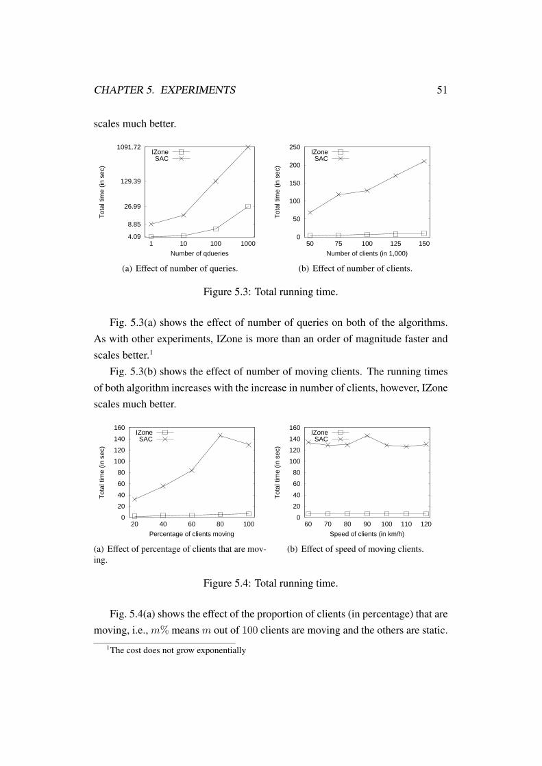
CHAPTER 5. EXPERIMENTS 51
scales much better.
4.09
8.85
26.99
129.39
1091.72
1 10 100 1000
Tot
al ti
me
(in s
ec)
Number of qdueries
IZoneSAC
(a) Effect of number of queries.
0
50
100
150
200
250
50 75 100 125 150
Tot
al ti
me
(in s
ec)
Number of clients (in 1,000)
IZoneSAC
(b) Effect of number of clients.
Figure 5.3: Total running time.
Fig. 5.3(a) shows the effect of number of queries on both of the algorithms.As with other experiments, IZone is more than an order of magnitude faster andscales better.1
Fig. 5.3(b) shows the effect of number of moving clients. The running timesof both algorithm increases with the increase in number of clients, however, IZonescales much better.
0
20
40
60
80
100
120
140
160
20 40 60 80 100
Tot
al ti
me
(in s
ec)
Percentage of clients moving
IZoneSAC
(a) Effect of percentage of clients that are mov-ing.
0
20
40
60
80
100
120
140
160
60 70 80 90 100 110 120
Tot
al ti
me
(in s
ec)
Speed of clients (in km/h)
IZoneSAC
(b) Effect of speed of moving clients.
Figure 5.4: Total running time.
Fig. 5.4(a) shows the effect of the proportion of clients (in percentage) that aremoving, i.e., m% means m out of 100 clients are moving and the others are static.
1The cost does not grow exponentially

CHAPTER 5. EXPERIMENTS 52
This figure shows similarity with Fig. 5.3(b), this is because when a client doesnot move, it does not report to the server about its location and location updates,hence the server does not need to calculate any thing for these clients. From thisperspective, when a larger number of clients are moving, it is equivalent to a largernumber of clients present in the network.
Fig. 5.4(b) shows the effect of the speed of moving clients. The performanceof the algorithms is not affected by the speed of moving clients and IZone consis-tently outperforms SAC.
5.4 Calculating Influence Zone
0
2
4
6
8
10
2 4 8 16 32 64
Initi
al c
alcu
latio
n tim
e (in
sec
)
Number of facilities (in 1,000)
IZoneSAC
(a) Effect of number of facilities on initial cal-culation
0
2
4
6
8
10
12
14
16
1 2 4 8 16 32 64
Initi
al c
alcu
latio
n tim
e (in
sec
)
k
IZoneSAC
(b) Effect of k on initial calculation
Figure 5.5: Influence zone calculation phase CPU time cost.
In this section, we demonstrate only the cost of first phase, i.e., influence zonecomputation time for IZone and pruning phase cost of SAC. We remark that theunpruned network is a superset of influence zone, i.e., it includes every pointsof the influence zone. We also remark that computing the influence zone is amore complicated task than computing the unpruned network due to the follow-ing reason. An unpruned network is a sub-network such that every client c thatlies outside it can be pruned, however, every client c′ that lies inside it may or maynot be pruned. In contrast, influence zone is a sub-network such that every clientc that lies outside it can be pruned and every client c′ that lies inside it cannot be

CHAPTER 5. EXPERIMENTS 53
pruned. This additional feature of influence zone that significantly reduces the to-tal running time makes the computational task of the first phase more challenging.
Fig. 5.5 shows the costs of first phase for both the algorithms for increasingnumber of facilities and increasing value of k. As stated earlier, influence zoneposes more complicated requirements, which implies that additional checks arerequired to compute the influence zone. Nevertheless, Fig. 5.5 shows that thecost of influence zone computation is almost the same as the cost of computingunpruned network. This indicates that our proposed technique computes a morecomplex region by incurring almost the same cost as incurred by SAC.

Chapter 6
Concluding Remark
6.1 Conclusion
In this thesis, we study the problem of continuous monitoring of reverse k nearestneighbors (RkNN) queries in spatial networks. RkNN query have received signif-icant research attention in the past few years due to its wide range of applications,and the continuous monitoring problem raise when inexpensive mobile devicesare widely used and popular.
We are the first to use the novel concept of influence zone in spatial networkswhich has many applications such as in location based services, marketing anddecision support systems. Since a client is the RkNN of the query point if and onlyif it is inside the influence zone, once the influence zone has been computed, weonly need to monitor the clients that lie inside the influence zone, this significantlyimproves the efficiency of monitoring.
Based on several non-trivial observations, we present an efficient algorithm tocompute the influence zone for both directed and undirected graphs. Our exten-sive experimental study demonstrates that our algorithm is more than an order ofmagnitude faster than the state-of-the-art RkNN monitoring algorithm.
54

CHAPTER 6. CONCLUDING REMARK 55
6.2 Future Work
In this thesis, we assume that the network is static, whilst in some real world casesit may change dynamically. For example, the expected travelling time required onroads is generally different during daytime and nighttime. In this case, the weightof edges (i.e. expected time required to go through) in the network is of interest,and when the condition changes, the influence zone becomes invalid and requiresre-calculation. How to avoid such expensive re-calculation could be an interestingresearch topic.

Bibliography
[1] Lars Arge, Mark de Berg, Herman J. Haverkort, and Ke Yi. The priorityr-tree: A practically efficient and worst-case optimal r-tree. In SIGMOD
Conference, pages 347–358, 2004.
[2] Rudolf Bayer. Binary b-trees for virtual memory. In SIGFIDET Workshop,pages 219–235, 1971.
[3] Rudolf Bayer and Edward M. McCreight. Organization and maintenance oflarge ordered indexes. In SIGFIDET Workshop, pages 107–141, 1970.
[4] Rimantas Benetis, Christian S. Jensen, Gytis Karciauskas, and SimonasSaltenis. Nearest neighbor and reverse nearest neighbor queries for mov-ing objects. In IDEAS, pages 44–53, 2002.
[5] Muhammad Aamir Cheema, Ljiljana Brankovic, Xuemin Lin, WenjieZhang, and Wei Wang. Multi-guarded safe zone: An effective techniqueto monitor moving circular range queries. In ICDE, pages 189–200, 2010.
[6] Muhammad Aamir Cheema, Xuemin Lin, Wenjie Zhang, and Ying Zhang.Influence zone: Efficiently processing reverse k nearest neighbors queries.In ICDE, pages 577–588, 2011.
[7] Muhammad Aamir Cheema, Xuemin Lin, Ying Zhang, Wei Wang, and Wen-jie Zhang. Lazy updates: An efficient technique to continuously monitoringreverse knn. PVLDB, 2(1):1138–1149, 2009.
[8] Muhammad Aamir Cheema, Wenjie Zhang, Xuemin Lin, and Ying Zhang.Efficiently processing snapshot and continuous reverse k nearest neighborsqueries. VLDB J., 21(5):703–728, 2012.
56

BIBLIOGRAPHY 57
[9] Muhammad Aamir Cheema, Wenjie Zhang, Xuemin Lin, Ying Zhang, andXuefei Li. Continuous reverse k nearest neighbors queries in euclidean spaceand in spatial networks. VLDB J., 21(1):69–95, 2012.
[10] Zaiben Chen, Heng Tao Shen, Xiaofang Zhou, and Jeffrey Xu Yu. Monitor-ing path nearest neighbor in road networks. In SIGMOD Conference, pages591–602, 2009.
[11] Hyung-Ju Cho and Chin-Wan Chung. An efficient and scalable approach tocnn queries in a road network. In VLDB, pages 865–876, 2005.
[12] Dong-Wan Choi, Chin-Wan Chung, and Yufei Tao. A scalable algorithmfor maximizing range sum in spatial databases. PVLDB, 5(11):1088–1099,2012.
[13] Ronald Fagin, Jurg Nievergelt, Nicholas Pippenger, and H. Raymond Strong.Extendible hashing - a fast access method for dynamic files. ACM Trans.
Database Syst., 4(3):315–344, 1979.
[14] Robert Geisberger, Peter Sanders, Dominik Schultes, and Daniel Delling.Contraction hierarchies: Faster and simpler hierarchical routing in road net-works. In WEA, pages 319–333, 2008.
[15] Diane Greene. An implementation and performance analysis of spatial dataaccess methods. In ICDE, pages 606–615, 1989.
[16] Antonin Guttman. R-trees: A dynamic index structure for spatial searching.In SIGMOD Conference, pages 47–57, 1984.
[17] Erik G. Hoel and Hanan Samet. Efficient processing of spatial queries inline segment databases. In SSD, pages 237–256, 1991.
[18] Ibrahim Kamel and Christos Faloutsos. Hilbert r-tree: An improved r-treeusing fractals. In VLDB, pages 500–509, 1994.
[19] James M. Kang, Mohamed F. Mokbel, Shashi Shekhar, Tian Xia, andDonghui Zhang. Continuous evaluation of monochromatic and bichromaticreverse nearest neighbors. In ICDE, pages 806–815, 2007.
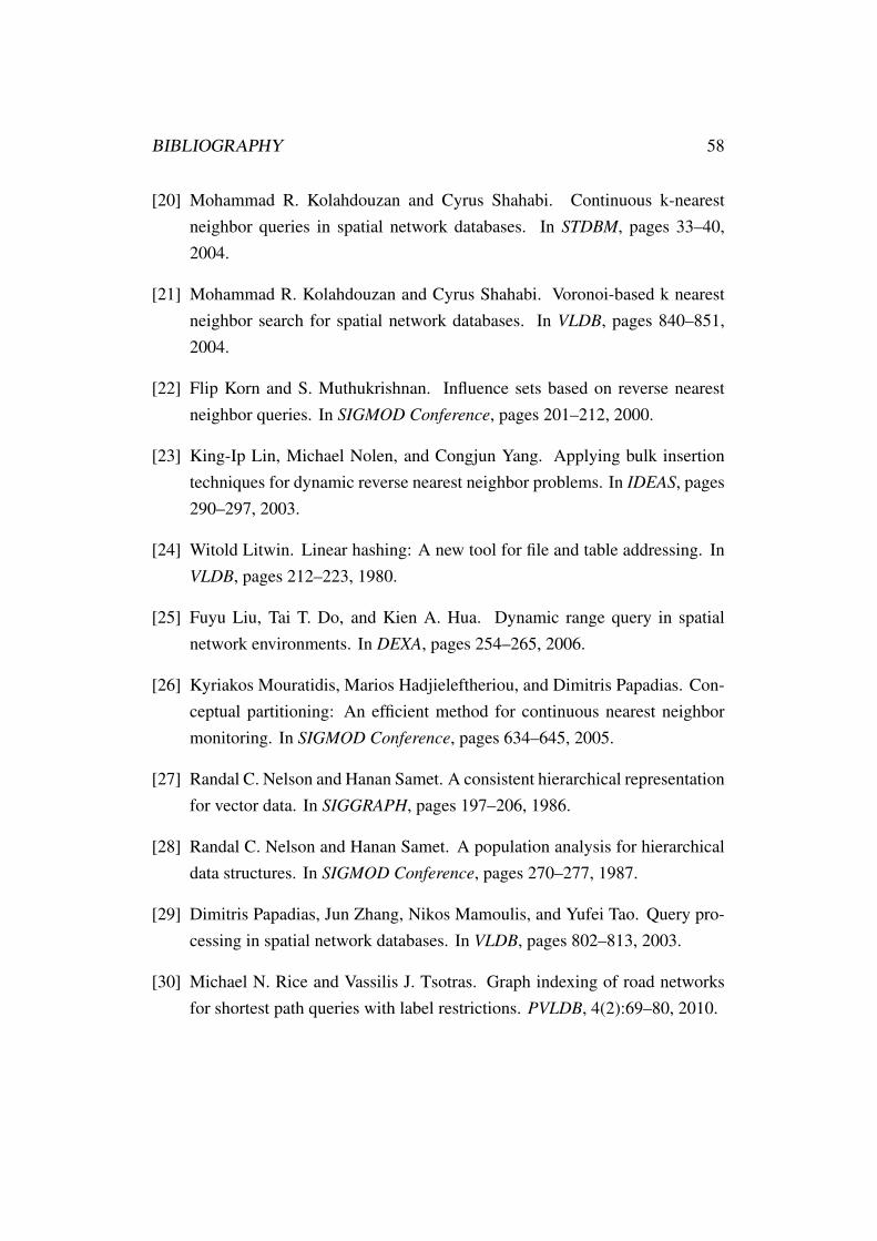
BIBLIOGRAPHY 58
[20] Mohammad R. Kolahdouzan and Cyrus Shahabi. Continuous k-nearestneighbor queries in spatial network databases. In STDBM, pages 33–40,2004.
[21] Mohammad R. Kolahdouzan and Cyrus Shahabi. Voronoi-based k nearestneighbor search for spatial network databases. In VLDB, pages 840–851,2004.
[22] Flip Korn and S. Muthukrishnan. Influence sets based on reverse nearestneighbor queries. In SIGMOD Conference, pages 201–212, 2000.
[23] King-Ip Lin, Michael Nolen, and Congjun Yang. Applying bulk insertiontechniques for dynamic reverse nearest neighbor problems. In IDEAS, pages290–297, 2003.
[24] Witold Litwin. Linear hashing: A new tool for file and table addressing. InVLDB, pages 212–223, 1980.
[25] Fuyu Liu, Tai T. Do, and Kien A. Hua. Dynamic range query in spatialnetwork environments. In DEXA, pages 254–265, 2006.
[26] Kyriakos Mouratidis, Marios Hadjieleftheriou, and Dimitris Papadias. Con-ceptual partitioning: An efficient method for continuous nearest neighbormonitoring. In SIGMOD Conference, pages 634–645, 2005.
[27] Randal C. Nelson and Hanan Samet. A consistent hierarchical representationfor vector data. In SIGGRAPH, pages 197–206, 1986.
[28] Randal C. Nelson and Hanan Samet. A population analysis for hierarchicaldata structures. In SIGMOD Conference, pages 270–277, 1987.
[29] Dimitris Papadias, Jun Zhang, Nikos Mamoulis, and Yufei Tao. Query pro-cessing in spatial network databases. In VLDB, pages 802–813, 2003.
[30] Michael N. Rice and Vassilis J. Tsotras. Graph indexing of road networksfor shortest path queries with label restrictions. PVLDB, 4(2):69–80, 2010.

BIBLIOGRAPHY 59
[31] Joao B. Rocha-Junior and Kjetil Nørvag. Top-k spatial keyword queries onroad networks. In EDBT, pages 168–179, 2012.
[32] Nick Roussopoulos, Stephen Kelley, and Fredeic Vincent. Nearest neighborqueries. In SIGMOD Conference, pages 71–79, 1995.
[33] Maytham Safar. K nearest neighbor search in navigation systems. Mobile
Information Systems, 1(3):207–224, 2005.
[34] Maytham Safar and Ahmad Al-Saleh. Pine based rnn queries in road net-works. In GeoInfo, pages 356–367, 2005.
[35] Maytham Safar, Dariush Ebrahimi, and David Taniar. Voronoi-based reversenearest neighbor query processing on spatial networks. Multimedia Syst.,15(5):295–308, 2009.
[36] Hanan Samet, Jagan Sankaranarayanan, and Houman Alborzi. Scalable net-work distance browsing in spatial databases. In SIGMOD Conference, pages43–54, 2008.
[37] Jagan Sankaranarayanan, Houman Alborzi, and Hanan Samet. Efficientquery processing on spatial networks. In GIS, pages 200–209, 2005.
[38] Jagan Sankaranarayanan and Hanan Samet. Query processing using distanceoracles for spatial networks. IEEE Trans. Knowl. Data Eng., 22(8):1158–1175, 2010.
[39] Jagan Sankaranarayanan, Hanan Samet, and Houman Alborzi. Path oraclesfor spatial networks. PVLDB, 2(1):1210–1221, 2009.
[40] Timos K. Sellis, Nick Roussopoulos, and Christos Faloutsos. The r+-tree:A dynamic index for multi-dimensional objects. In VLDB, pages 507–518,1987.
[41] Mehdi Sharifzadeh and Cyrus Shahabi. Vor-tree: R-trees with voronoi dia-grams for efficient processing of spatial nearest neighbor queries. PVLDB,3(1):1231–1242, 2010.

BIBLIOGRAPHY 60
[42] Ioana Stanoi, Divyakant Agrawal, and Amr El Abbadi. Reverse nearestneighbor queries for dynamic databases. In ACM SIGMOD Workshop on
Research Issues in Data Mining and Knowledge Discovery, pages 44–53,2000.
[43] Huan-Liang Sun, Chao Jiang, Jun-Ling Liu, and Limei Sun. Continuousreverse nearest neighbor queries on moving objects in road networks. InWAIM, pages 238–245, 2008.
[44] David Taniar, Maytham Safar, Quoc Thai Tran, J. Wenny Rahayu, andJong Hyuk Park. Spatial network rnn queries in gis. Comput. J., 54(4):617–627, 2011.
[45] Yufei Tao, Dimitris Papadias, and Xiang Lian. Reverse knn search in arbi-trary dimensionality. In VLDB, pages 744–755, 2004.
[46] Quoc Thai Tran, David Taniar, and Maytham Safar. Reverse k nearest neigh-bor and reverse farthest neighbor search on spatial networks. T. Large-Scale
Data- and Knowledge-Centered Systems, 1:353–372, 2009.
[47] Haojun Wang and Roger Zimmermann. Snapshot location-based query pro-cessing on moving objects in road networks. In GIS, page 50, 2008.
[48] Wei Wu, Fei Yang, Chee Yong Chan, and Kian-Lee Tan. Continuous reversek-nearest-neighbor monitoring. In MDM, pages 132–139, 2008.
[49] Wei Wu, Fei Yang, Chee Yong Chan, and Kian-Lee Tan. Finch: evaluatingreverse k-nearest-neighbor queries on location data. PVLDB, 1(1):1056–1067, 2008.
[50] Tian Xia and Donghui Zhang. Continuous reverse nearest neighbor moni-toring. In ICDE, page 77, 2006.
[51] Xiaokui Xiao, Bin Yao, and Feifei Li. Optimal location queries in roadnetwork databases. In ICDE, pages 804–815, 2011.
[52] Congjun Yang and King-Ip Lin. An index structure for efficient reversenearest neighbor queries. In ICDE, pages 485–492, 2001.