tag unit 5.3 - supplementary economic modelling · 4.4 luti models 6 4.5 s-cge models 7 ... 2.1.5...

https://www.gov.uk/transport-analysis-guidance-webtag

https://www.gov.uk/transport-analysis-guidance-webtag

mailto:[email protected]

Contents

1 Introduction 1

2 Key Messages 1

3 Rationale for undertaking Supplementary Economic Modelling 2

4 Overview of Supplementary Economic Models 3

4.1 Introduction 3 4.2 Additionality models 4 4.3 Reduced-form models 5 4.4 LUTI models 6 4.5 S-CGE models 7

5 Model Selection Guidance 7

6 Model Robustness Criteria 9

6.1 Introduction 9 6.2 Economic Principles 9 6.3 Baseline Assumptions 10 6.4 Model Geographic Scope 10 6.5 Transport Accessibility Improvement 11 6.6 Macroeconomic Projections 11 6.7 Model Structure 11 6.8 Model Parameters 11 6.9 Displacement Effects 12 6.10 Estimating Social Welfare Impacts 13 6.11 Complementary Interventions 15 6.12 Sensitivity Testing 16 6.13 Realism Tests 16 6.14 Consistency with Conventional Appraisal Methods 16 6.15 Independent Peer Review 17

7 Reporting Supplementary Economic Modelling 17

7.2 Economic Case 17 7.3 Strategic Case 18

8 References 19

TAG Unit M5.3 Supplementary Economic Modelling

Page 1

1 Introduction 1.1.1 This Unit provides high-level guidance to inform the estimation, reporting and peer review of

‘Supplementary Economic Models’. Supplementary Economic Models are defined here as non-standard methods to estimate the economic impact of transport schemes including Additionality models, Reduced-form models, Land-Use Transport Interaction (LUTI) models and Spatial-Computable General Equilibrium (S-CGE) models.

1.1.2 This guidance should be used by technical project managers and consultants to inform the scoping, undertaking and reporting of Supplementary Economic Modelling, both for individual transport schemes and packages of schemes. It should also be used to inform the peer review of Supplementary Economic Models and by Government analysts to inform the weight placed on this analysis as part of a scheme’s Business Case.

1.1.3 This Unit is structured as follows:

• Section 2 summarises the key messages of this unit; • Section 3 explains the circumstances when Supplementary Economic Modelling may be

appropriate; • Section 4 summarises the main categories of Supplementary Economic Models; • Section 5 provides guidance to inform model selection; • Section 6 sets out criteria for assessing the robustness of Supplementary Economic Models;

and • Section 7 provides guidance how model results and assumptions should be reported in the

Business Case.

2 Key Messages 2.1.1 ‘Supplementary Economic Models’ are defined here as non-standard methods of estimating the

impact of transport schemes on the economy (i.e. deviating from methods set out in the A1 and A2 Units of WebTAG). Examples of Supplementary Economic Modelling include Additionality models, Reduced-form models, LUTI models, and S-CGE models.

2.1.2 Most Supplementary Economic Models assess how transport schemes impact on the spatial distribution of the economy. Given the challenges associated with appraising these impacts and the difficulty of validating these models, they should be used to supplement rather than replace conventional appraisal methods (set out in TAG Units A1 and A2).

2.1.3 Supplementary Economic Modelling may be undertaken:

• To quantify and value user-benefits for schemes impacting the spatial distribution of the economy;

• To capture a broader range of Wider Economic Impacts than those provided for in the A2 Units of TAG, such as productivity gains from localisation effects (increased connectivity of single-industry clusters);

• To obtain context-specific estimates of welfare impacts set out in the A2 Units of TAG, such as mode-specific agglomeration elasticities; or

• To estimate sub-national impacts, such as changes in local employment and GDP.

2.1.4 Where Supplementary Economic Modelling has been undertaken it is necessary that the following are undertaken:

• First, it is necessary to report the extent to which each of the ‘model robustness criteria’ in section 6 have been addressed. This will inform the weight placed on the analysis in the


Page 2

scheme’s Business Case. It is recognised that it may not be proportionate or feasible for all of the modelling robustness criteria to be addressed for a given scheme.

• Second, where Supplementary Economic Modelling has been used to estimate a scheme’s impact on GDP it is required that welfare estimates are obtained using the same assumptions. The purpose of this is to ensure consistency between the evidence informing the Strategic and Economic Cases. Section 6.10 provides guidance on how Supplementary Economic Models can be used to obtain social welfare estimates.

• Third, where Supplementary Economic Modelling is used to estimate sub-national economic impacts it is required that equivalent national impacts are estimated using the same assumptions. The purpose of this is to provide decision-makers with evidence about potential displacement effects.

2.1.5 As with the wider economic impacts guidance, the default assumption is 100% displacement, in other words user benefits are assumed to capture fully the economic impacts of a transport investment. Only where context specific evidence is presented which demonstrates a supply side effects in labour, product or capital markets will there be national economic impacts over and above those captured by user benefits.

2.1.6 Given the high level of uncertainty associated with Supplementary Economic Models, estimates from these models should not be reported in a scheme’s initial or adjusted benefit-cost ratios but instead should be reported separately as ‘sensitivity tests’.

3 Rationale for undertaking Supplementary Economic Modelling 3.1.1 This section provides guidance to inform when Supplementary Economic Modelling may be

appropriate.

3.1.2 The Department’s preferred approach to estimate a scheme’s economic impacts is to use methods set out in TAG Units A1 and A2. The rationale for this is as follows:

• First, the primary focus of transport appraisal should be to estimate a scheme’s impact on social welfare (rather than to appraise GDP impacts). Units A1 and A2 provide methods to estimate social welfare benefits associated with boosting the economy.

• Second, it is not necessary to undertake Supplementary Economic Modelling to estimate a scheme’s GDP impact as this can be inferred from the welfare-based appraisal. Table 1 summarises each of those welfare benefits covered in TAG Units A1 and A2 and their corresponding GDP impacts. The central estimates for a scheme’s impacts on GDP and social welfare can be estimated by summing those impacts in the relevant columns, excluding benefits associated with dependent developments to avoid double-counting. It should be noted that this table doesn’t include social and environmental impacts which may contribute to both welfare and GDP.

• Third, methods set out in TAG Units A1 and A2 have been externally peer reviewed and are therefore assessed to be robust.


Page 3

Table 1 – Correspondence between national welfare and GDP impacts Impacts (TAG Unit) Welfare Impact GDP Impact User Benefits (A1.3) User benefits from business,

commuting and leisure trips Business user benefits

Induced Investment (A2.2) Dependent Development*

Land value uplift

Additionality modelling (M3.5)

Output effects with Imperfect Competition

10% of Business User Benefits 10% of Business User Benefits

Employment Effects (A2.3) Labour Supply Impacts

40% of change to GDP

Change in GDP

Movement to More/Less Productive Jobs

30% of change to GDP Change in GDP

Productivity Impacts (A2.4) Agglomeration Economies (incl. static and dynamic clustering)

Agglomeration Impacts

Agglomeration Impacts

* Note that GDP and welfare benefits associated with dependent developments should not be added to user benefits since this would result in benefits being double-counted.

3.1.3 Nevertheless in some circumstances it may be desirable to undertake Supplementary Economic Modelling to estimate a scheme’s welfare and GDP impacts. For example, it may be appropriate to undertake Supplementary Economic Modelling:

• To quantify and value user-benefits for schemes impacting the spatial distribution of the economy;

• To capture a broader range of Wider Economic Impacts than those provided for in the A2 Units of TAG, such as productivity gains from localisation effects (increased connectivity of single-industry clusters);

• To obtain context-specific estimates of welfare impacts set out in the A2 Units of TAG, such as mode-specific agglomeration elasticities; or

• To estimate sub-national impacts, such as changes in local employment and GDP.

3.1.4 As described in TAG Unit A2.1, the default assumption for all transport appraisals is 100% displacement, in other words user benefits are assumed to capture fully the national economic impacts of a transport investment. Departures from the default assumption must be justified through the presentation of context specific evidence which demonstrates a supply side effect in either the labour, product or capital markets

3.1.5 The default assumption in the labour, capital and product markets is that resources are fully used; wages, return on capital and prices are assumed to be fully flexible to ensure there is no unemployment, idle physical/financial capital or unsold output, respectively. Changes in the demand for labour, capital or products will in and of itself not improve economic performance. They will only serve to displace economic activity from other locations or industries. This default assumption should be the starting point for all supplementary economic modelling.

3.1.6 The decision to undertake Supplementary Economic Modelling should be informed by the expected impacts and justification for these set out in the scheme’s Economic Narrative. Further guidance about the Economic Narrative can be found in TAG Unit A2.1.

4 Overview of Supplementary Economic Models

4.1 Introduction

4.1.1 This section provides an overview of the main categories of Supplementary Economic Models: Additionality models; Reduced-form models; LUTI models; and S-CGE models. It should be noted


Page 4

that these categories of models are not mutually exclusive, for example estimates from Reduced-form models may be used to inform S-CGE models. More detailed discussions about the different categories of Supplementary Economic Models can be found in the reports ‘Transport investment and Economic Performance’ (DfT, 2014) and ‘Assessment of Methods for Modelling and Appraisal of the Sub-National, Regional and Local Economy Impacts of Transport’ (DfT, 2013).

4.2 Additionality models

4.2.1 ‘Additionality models’ (or ‘bottom-up’ approaches) are defined here as approaches to estimate the impact of government interventions on net GDP or jobs making explicit judgements about leakage, deadweight, displacement and multiplier effects. These terms are defined in Box 1.

4.2.2 Additionality models typically rely on local evidence to assess how the transport improvement will impact the economy. This may include analysing descriptive statistics for the local economy (e.g. unemployment rates and the industrial split of production), interviews with stakeholders to ascertain how they will respond to the transport improvement and consideration of local growth and development plans.

4.2.3 Additionality models are often used to value the increase in net GDP or jobs associated with developments enabled by local transport improvements (known as ‘dependent developments’). The net GDP and jobs impacts can be valued by first estimating the gross GDP or jobs of businesses occupying these developments and second assessing the extent to which these impacts are ‘additional’. Each of these steps is discussed in turn.

4.2.4 First, the standard approach to estimate the gross GDP and jobs associated with dependent developments is as follows:

• Identify potential dependent developments; • Estimate the floor space covered by these developments; • Estimate the gross number of jobs located at these developments by making assumptions

about occupancy rates, for example using estimates produced by the Homes and Communities Agency (2015); and

• Estimate the gross GDP associated with the developments by multiplying the gross jobs impact by the assumed GDP per person.

4.2.5 Second, the net GDP and jobs impacts can then be estimated by adjusting the gross GDP and

jobs impacts to account for leakage, deadweight, displacement and multiplier effects. This should be done based on context-specific information for the scheme in question. For example, TAG Unit

Box 1 – Terminology associated with additionality models

• Additionality – the extent to which an increase in GDP or jobs in a given target area is higher than it would otherwise have been as a result of Government intervention. Estimates of the local impact need to be modified to account for leakage, deadweight, displacement and multiplier effects.

• Leakage effects – the extent to which GDP or jobs impacts take place outside of target area of the Government intervention

• Deadweight effects – the extent to which the GDP or jobs impacts would have occurred anyway without the Government intervention.

• Displacement effects– extent to which increased jobs and GDP in one location results in lower jobs or GDP elsewhere in the target area.

• Multiplier effects – the extent to which a rise in GDP or jobs is ‘multiplied’ by increased business and consumer spending, known as indirect and induced multiplier effects respectively.


Page 5

A2.2 provides guidance for assessing the level of deadweight and displacement associated with dependent developments. In addition, evaluation evidence from the Department for Business Innovation and Skills (BIS) (2009a) may be used to inform estimates for leakage, deadweight, displacement and multiplier effects at the regional and sub-regional levels. Given that displacement is expected to be greater at the national than regional or sub-regional levels, displacement estimates from BIS (2009a) may be used as lower-bounds for the national impact.

4.2.6 Additionality models typically assume that transport schemes are only able to raise net GDP or jobs in the short-term (since these impacts are assumed to become deadweight in the longer-term). Evidence from the Regional Development Agency Impact Evaluations suggests that net GDP and jobs benefits should be assumed to persist for 10 years; however, the Department for Communities and Local Government (CLG) have previously adopted a more cautious assumption of 5 years (see CLG, 2010).

4.2.7 When using Additionality models it is recommended that sensitivity testing is undertaken estimating the scheme’s impact on net GDP and jobs under a range of plausible assumptions for deadweight, displacement, leakage and multiplier effects.

4.2.8 There are a number of sources of guidance to inform additionality modelling, for example:

• Annex 1 of HM Treasury (2011) ‘The Green Book: appraisal and evaluation in Central Government’

• Department for Business Innovation and Skills (2009a) ‘Research to improve the • assessment of additionality’ • Department for Business Innovation and Skills (2009b) ‘Guidance for using additionality

benchmarks in appraisal’ • English Partnership (2008) ‘Additionality Guide: A standard approach to assessing the

additional impact of interventions’ • Homes and Communities Agency (2014) ‘Additionality Guide: Fourth Edition 2014’ • Department for Communities and Local Government (2010) ‘Valuing the Benefits of

Regeneration, Economics paper 7: Volume 1 – Final Report’

4.3 Reduced-form models

4.3.1 In transport economics, Reduced-form models (or ‘econometric models’) use empirical estimates for the relationship between effective densities and economic activity to estimate the impact of a given scheme. ‘Effective density’ is defined here as a metric for the number of households or businesses that can be accessed from a given location, down-rating employment or businesses in more distant regions by a decay factor.

4.3.2 Reduced-form models can be used to estimate the impact of a proposed transport scheme on economic activity as follows:

• First it’s necessary to obtain elasticities of economic activity with respect to effective densities (either from existing empirical studies or original research);

• Second it’s necessary to estimate the change in effective densities for locations impacted by the transport scheme; and

• Third, the scheme’s impact on economic activity can be calculated using the elasticity and estimates for its impact on effective densities.

4.3.3 One use of reduced-form modelling is to estimate agglomeration benefits. The default approach for estimating agglomeration benefits is to follow guidance in TAG Unit A2.4 based on agglomeration elasticities from Graham et al. (2009). Nevertheless in some circumstances it may be desirable to undertake Supplementary Economic Modelling to estimate agglomeration benefits using alternative elasticities to inform sensitivity tests. For example:


Page 6

• It may be desirable to obtain context-specific agglomeration elasticities if the national-average elasticities from Graham et al. (2009) are judged to be unrealistic. The elasticities quoted in TAG Unit A2.4 assume a linear relationship between agglomeration benefits and effective densities. If the true relationship were non-linear then using the elasticities from Graham et al. (2009) may under- or over-estimate agglomeration benefits for the very largest cities; or

• It may be desirable to estimate new elasticities to appraise ‘localisation effects’. These effects represent the productivity gains from cities becoming more specialised in specific industries. As a consequence it may be desirable to appraise ‘localisation effects’ for inter-city transport schemes. By contrast, elasticities from Graham et al (2009) are capable of estimating ‘urbanisation effects’ (productivity gains from increased connectivity of multi-sector clusters) and are therefore more relevant for appraising intra-city schemes.

4.3.4 The rationale for using alternative agglomeration elasticities to those from Graham et al. (2009) should be justified in the scheme’s Economic Narrative.

4.3.5 Section 6.8 sets out some of the potential biases associated with spatial econometrics and how they can be addressed.

4.4 LUTI models

4.4.1 Land-Use Transport Interaction (LUTI) models have separate land-use and transport models. The term ‘land-use’ in this context refers not only to the construction of new developments but also to the spatial re-organisation of the economy such as changes in the locations of firms and businesses. The purpose of a LUTI model is to understand how a transport investment will impact upon land use change. Some LUTI models may be capable of capturing the two-way interaction between the transport network and the land-use. However, in many instances the LUTI models will not capture the feedback between land-use and the transport network.

4.4.2 There are a variety of LUTI models available with different levels of geographic coverage, granularity and assumptions. Inter-regional LUTI models typically use a multi-region input-output framework or a production function approach. By contrast, Wegener (2011) identifies three genres of intra-regional LUTI models:

• Location models which take changes in trade flows from an input-output framework as an indicator of changes in industry location;

• Bid-rent location models that have firms acting as profit-maximisers choosing locations given land prices (where land prices are determined endogenously within the model); and

• Utility-based location models where firms choose locations to maximise their utility taking into account factors such as access to labour and product markets.

4.4.3 Whenever LUTI modelling is undertaken it should be done in line with Supplementary Economic Modelling guidance. For example, LUTI models may be required to estimate wider economic benefits from movement to more/less productive jobs and dynamic clustering set out in TAG Units A2.3 and A2.4 respectively. In addition, LUTI models may be used to estimate economic impacts not covered elsewhere in WebTAG such as the Integrated Land-Use/Transport Economic Efficiency Analysis (ULTrA) described in Simmonds et al (2012).

4.4.4 The following documents provide further discussion about LUTI models:

• Chapter 5 from SACTRA (2001) ‘Transport and the Economy’ • DfT (2014) 'Supplementary Guidance: Land Use/Transport Interaction Models' • Wegener (2014) ‘Land-Use Transport Interaction Models’ • Wegener (2011) ‘Transport in spatial models of economic development’


Page 7

4.5 S-CGE models

4.5.1 Spatial-Computable General Equilibrium (S-CGE) models are large-scale numerical models that attempt to explain the key interactions between households, firms and government (including intertemporal and spatial interactions). They are referred to as ‘general equilibrium’ models as they explicitly model interactions between multiple markets, unlike ‘partial equilibrium’ models which consider transport-using markets in isolation.

4.5.2 One of the key characteristics of S-CGE models is that prices and wages are assumed to adjust such that supply and demand in all markets remain in equilibrium. Hence they implicitly take into account that demand-side shocks may be partially crowded out by changes in prices or wages. In addition, these models are capable of predicting how changes in the relative prices of different goods and services impact on the industrial mix of production.

4.5.3 The following texts provide further discussion about S-CGE models:

• Bröcker J. and Mercenier J. (2011) ‘General equilibrium models for transportation economies’

• Bröcker J. (2015) ‘Spatial computable general equilibrium analysis’

• Burfisher M. E. (2011) ‘Introduction to computable general equilibrium models’

• Dixon P. B. (2013) ‘Handbook of computable general equilibrium modelling’

• Ginsburgh V. and Keyzer M. (1997) ‘The Structure of Applied General Equilibrium’

• Hosoe N. and Gasawa K. Hideo Hashimoto (2010) ‘Textbook of Computable General Equilibrium Modelling’

• Shoven J.B. and Whalley J. (1984) ‘Applied general equilibrium models of taxation and international trade’

5 Model Selection Guidance 5.1.1 This section provides high-level guidance to inform which categories of Supplementary Economic

Models are most appropriate for a given scheme.

5.1.2 The Department’s view is that there is no single best approach to capture all of the economic impacts of transport improvements. Rather, different methods may be applicable to different contexts depending on the scheme’s anticipated impacts (set out in the Economic Narrative) and proportionality considerations. Table 2 provides a comparison of some key strengths, weaknesses and uses of different Supplementary Economic Models.


Page 8

Table 2 – Comparison of the strengths, weakness and uses of Supplementary Economic Models

Name Strengths Weaknesses Appropriateness for use

Additionality models

Relies on local evidence including interviews with stakeholders and growth plans. Doesn’t require an existing model therefore appropriate for smaller schemes.

Subjective judgements required to determine additionality factors, potentially resulting in optimism bias.

Best suited to small-scale schemes, particularly those enabling dependent developments.

Reduced-form models

A large body of evidence already exists for the empirical relationship between effective densities and productivity.

Simpler than developing LUTI or S-CGE models from scratch.

Doesn’t necessarily take into account local constraints on economic growth. Secondary modelling required to estimate displacement effects. Risks that elasticities may not represent the causal impact of transport schemes on economic activity.

Particularly relevant for estimating agglomeration benefits (e.g. using context-specific elasticities)

LUTI models Capable of estimating a wide range of impacts including changes in the level and location of employment, investment, GDP and welfare. Capable of capturing economic impacts at a granular level (though level of granularity differs between models). May be capable of estimating the two-way interaction between land-use and transport models. Takes into account local constraints on economic growth (e.g. availability of suitable land for developments and suitably skilled labour).

Complex, data-intensive models requiring numerous modelling judgements (e.g. for inter-regional trade linkages). Depending on design, may not be capable of capturing the two-way interaction between land-use and transport models.

Useful for appraising local impacts (granularity of results depends on the model).

Some models capable of estimating national impacts including dynamic clustering, movement to more/less productive jobs and multiplier effects

Spatial General Equilibrium (S-CGE) models

Capable of estimating a wide range of impacts including changes in the level and location of employment, investment, GDP and welfare. Take into account local constraints on economic growth; however, typically using less granular data than LUTI models Explicitly model price and wage change.

Complex, data-intensive models requiring numerous modelling judgements (e.g. inter-regional trade linkages). Typically not capable of capturing the two-way interaction between land-use and transport models. Model zones are typically less granular than LUTI models.

Capable of estimating national impacts including multiplier effects and dynamic clustering

Only proportionate for the largest schemes due to cost.


Page 9

6 Model Robustness Criteria

6.1 Introduction

6.1.1 This section sets out the model robustness criteria and reporting requirements for Supplementary Economic Models. It is a requirement that the extent to which each of these criteria have been addressed (if at all) should be reported in the Economic Impacts Report. The extent to which these criteria have been addressed will inform the weight placed on the analysis in the scheme’s Business Case. Nevertheless it is recognised that it may not be proportionate or feasible for all of the modelling robustness criteria to be addressed for a given scheme.

6.1.2 These criteria should not be viewed as an exhaustive list of issues to consider as part of a peer review.

6.2 Economic Principles

6.2.1 In the first instance it is recommended that Supplementary Economic Models adopt the economic principles underlying WebTAG (see Box 2). For the majority of transport schemes these principles should be appropriate.

6.2.2 Nevertheless, in some circumstances it may be relevant to adopt more sophisticated economic principles in the appraisal. For example, when appraising the benefits from airport expansion it may be appropriate to assess the impacts on UK trade, foreign direct investment and net migration.

6.2.3 Where an appraisal is using different economic principles to those adopted in WebTAG it is necessary to report how they differ. Greater confidence will be placed in analyses which are based on credible economic theories and are relevant for the context in which they’re being used.


Page 10

6.3 Baseline Assumptions

6.3.1 It is necessary to report the assumptions underlying the core (or without-scheme) scenario. Greater weight will be placed on modelling where the same assumptions are adopted in the Supplementary Economic Model as those adopted in the transport model. M4 – Forecasting and Uncertainty provides guidance about which developments and transport schemes should be assumed to occur in the core scenario.

6.4 Model Geographic Scope

6.4.1 It is necessary to report the geographic scope of the modelled area and the sizes of modelled zones. Greater confidence will be placed in analysis where the geographic scope of the modelled area captures the majority of the expected impacts of the scheme including displacement effects. In addition, greater confidence will be placed in models with relatively small zones, particularly in the locality of the scheme.

Box 2: Economy Principles underlying WebTAG Supply-side assumptions – currently WebTAG implicitly assumes that the economy is in ‘full employment’, with wages assumed to adjust to eliminate involuntary unemployment. This simplifying assumption is broadly consistent with guidance in the Green Book (HM Treasury, 2011) which states that ‘if there are no grounds for expecting a proposal to have a supply side effect, any increase in government expenditure would result in a matching decrease in private expenditure, (known as ‘crowding out’)’. The assumption of ‘full employment’ has a number of implications for transport appraisal:

• First, it implies that increase in public- or private-sector spending on goods and services cannot raise total employment but instead displaces labour from elsewhere in the economy. As a consequence, WebTAG does not provide methods for appraising jobs and GDP associated multiplier effects or increased construction activity as these are assumed to have no net national impacts; and

• Second, it implies that the only means by which the government can raise total output is through supply-side measures such as boosting productivity or removing obstacles to people entering the labour market. Hence the A2 units provide the only methods to appraise supply-side impacts associated with transport investments (e.g. agglomeration benefits and labour supply effects).

Market failures and Government Distortions – WebTAG recognises that there are a number of market failures and government distortions in the market for goods, labour and land. For example:

• Externalities – A2.4 – Productivity Impacts provides guidance for appraising the productivity benefits from increased clustering of businesses and households (known as ‘agglomeration benefits’). Other Units also provide guidance for appraising welfare impacts associated with environmental and social externalities (e.g. impacts on air quality and accidents from increased car travel);

• Market structure – currently WebTAG allows for both perfect and imperfect competition in markets for goods and services. The method for estimating Transport User Benefits in A1.3 – User and Provider Impacts implicitly assumes that businesses compete in perfectly competitive markets. Nevertheless A2.2 – Induced Investment provides guidance to estimate Wider Economic Impacts associated with imperfect competition in markets for goods and services;

• Land rationing – It is recognised in A2.2 – Induced Investment that planning policies may result in an inefficiently low level of construction activity. As a consequence the unit provides guidance to estimate the welfare benefits associated with enabled developments; and

• Tax distortions – even where there are no private welfare benefits from increased GDP (due to offsetting welfare losses) there may be welfare benefits from increased tax revenue. A2.3 - Employment provides guidance to estimate the tax wedges associated with labour supply effects and movement to more/less productive jobs.

International linkages – the methods in WebTAG are not intended to capture the impact of transport.schemes on trade, foreign investment and net migration.


Page 11

6.5 Transport Accessibility Improvement

6.5.1 It is necessary to report the following information relating to the transport accessibility improvement:

• How the transport accessibility improvement has been estimated; • How the transport accessibility improvement has been input into the model (e.g. change in

generalised travel costs, user benefits, travel time savings or productivity); • Whether the transport accessibility improvement input to the model is consistent with that

used to estimate Transport User Benefits; and • Whether analysis has been undertaken to iteratively run the land-use model with the transport

model and, if so, how many times.

6.5.2 Greater confidence will be placed in models where:

• The transport accessibility improvement has been estimated using a well-specified transport model, that is, the transport modelling is consistent with guidance in the WebTAG Modelling units;

• The same estimates of the transport accessibility improvements, used to calculate Transport User Benefits, are used as inputs into the Supplementary Economic Model; and

• There is evidence to suggest that further iterations of the Supplementary Economic Model with the transport model aren’t expected to significantly affect the results.

6.6 Macroeconomic Projections

6.6.1 It is necessary to report all of the key projections underpinning the model, present their sources (if relevant) and state whether they are consistent with the assumptions informing the transport model. Where projections have been estimated by the project team, it is necessary to set out the methodology and assumptions underpinning these. Greater confidence will be placed in models where projections are consistent with those informing the transport model, for example using estimates from TEMPro (the Trip End Model Presentation Program), or are based on other official Government projections.

6.7 Model Structure

6.7.1 It is necessary to report each of the key mathematical relationships underpinning the model, providing a reasoned explanation for each. Greater confidence will be placed in models where it can be demonstrated that the model structure is consistent with credible economic principles and best-practice (e.g. consistent with relationships set out in WebTAG or other empirical studies).

6.8 Model Parameters

6.8.1 It is necessary to report all the key parameters underpinning Supplementary Economic Models including sources and evidence indicating the level of uncertainty associated with these estimates. Greater confidence will be placed in model parameters where it can be demonstrated that:

• The parameters are consistent with the default assumptions set out elsewhere in WebTAG (unless it can be justified that alternative estimates are more robust or up-to-date);

• The parameters are robust, for example excluding outliers and satisfying tests for statistical significance;

• The parameters have narrow confidence interval; • The parameter are plausible compared to results from other empirical studies (e.g.

parameters do not represent outliers compared to other studies); and • The parameters are not invalidated by the Lucas Critique (Lucas, 1976), for example they are

estimated using recent data from the UK.


Page 12

6.8.2 See the example Uncertainty Log in Appendix A of M4 – Forecasting and Uncertainty for a potential template how this information could be reported.

6.8.3 Where spatial econometrics has been undertaken it is also necessary to demonstrate that estimates are not influenced by omitted variable bias, simultaneity or multicollinearity. Each of these issues are discussed below:

Omitted variable bias 6.8.4 Omitted variable bias may occur where there are area-specific factors impacting on economic

activity which are not controlled for in the model. For example, when estimating agglomeration elasticities it is necessary to control for differences in average skills between regions (since highly-skilled people often move to areas with higher effective densities). This can be achieved by including fixed effects or measures of average skills as independent variables in the regression.

Simultaneity bias 6.8.5 Simultaneity bias may occur if areas with higher effective densities experience larger transport

investments. In which case, the coefficient on effective density may not accurately represent the causal impact of the transport scheme on economic activity. Simultaneity bias may be addressed by using fixed effect estimation or instrumental variables.

Multicollinearity 6.8.6 Multicollinearity bias may occur if separate independent variables for effective densities by

different modes of transport have been included in the regression. These effective densities are likely to be highly correlated with each other, resulting in their respective coefficients changing erratically in response to small changes in the model or the data. This issue may be addressed by including only one independent variable for effective densities in the regression or interpreting coefficients on each of the effectivity densities collectively (rather than interpreting each in isolation).

6.9 Displacement Effects

6.9.1 It is necessary to report how displacement effects have been accounted for in the Supplementary Economic Modelling, detailing the methods used to estimate these impacts. Displacement reflects the extent to which an increase in economic activity in one location is partially or fully offset by reductions elsewhere. For example, an increase in employment in one location may displace jobs from elsewhere in the country.

6.9.2 There are a variety of approaches to model displacement effects, for example:

• Additionality models account for displacement by down-rating gross GDP and jobs impacts by a ‘displacement factor’ informed by context-specific information and evaluation evidence;

• Reduced-form models do not take into account displacement effects unless secondary modelling is undertaken (e.g. estimating how households and businesses move around the country in response to the transport scheme); and

• Some LUTI models account for displacement by imposing labour market closure (i.e. assuming that transport schemes can impact the location but not level of employment).

6.9.3 Greater confidence will be placed in analysis which can demonstrate that displacement effects

have been robustly modelled.


Page 13

6.10 Estimating Social Welfare Impacts

6.10.1 Where Supplementary Economic Modelling has been used to estimate a scheme’s impact on economic activity (e.g. GDP or jobs) it is necessary to report the equivalent national social welfare impact. The purpose of this is to ensure that figures informing the scheme’s Strategic and Economic cases have been estimated on a consistent basis. These ‘supplementary’ estimates for a scheme’s social welfare impacts may then be used to inform its value for money rating, discussed in section 7.

6.10.2 There are a variety of approaches which might be used to estimate a scheme’s impact on social welfare. This section presents two approaches to convert model outputs to welfare estimates, referred to as the ‘bottom-up’ and ‘top-down’ approaches. The ‘bottom-up’ approach is the preferred method where Supplementary Economic Modelling has been undertaken to estimate Wider Economic Impacts using alternative assumptions to those recommended in the A2 Units. Nevertheless, where the outputs from Supplementary Economic Models do not correspond to Wider Economic Impacts it may be more appropriate to use the ‘top-down’ approach. It should be noted that there may be other approaches to estimate welfare impacts using Supplementary Economic Models such as the Integrated Land-Use/Transport Economic Efficiency Analysis set out in Simmonds et al (2012).

6.10.3 Having obtained welfare estimates from Supplementary Economic Models, it is then necessary to assess whether these impacts are additional to other appraised welfare impacts, that is, they can be added together without double-counting. This is necessary when assessing a scheme’s value for money category.

Bottom-up approach 6.10.4 The bottom-up approach is to obtain ‘supplementary’ estimates for those Wider Economic Impacts

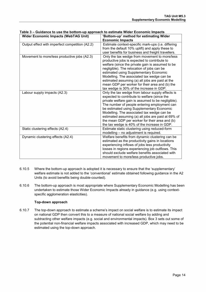
included in the A2 Units. For example, TAG Units A2.3 and A2.4 states how Supplementary Economic Models may be used to estimate movement to more/less productive jobs effects and dynamic clustering. In addition other Wider Economic Impacts may be estimated using results from Supplementary Economic Models, for example, context-specific elasticities to estimate agglomeration benefits. Table 3 summarises how Supplementary Economic Modelling may be used to obtain bottom-up estimates for each of the Wider Economic Impacts currently in WebTAG.


Page 14

Table 3 – Guidance to use the bottom-up approach to estimate Wider Economic Impacts

Wider Economic Impacts (WebTAG Unit) ‘Bottom-up’ method for estimating Wider Economic Impacts

Output effect with imperfect competition (A2.2) Estimate context-specific mark-ups (i.e. differing from the default 10% uplift) and apply these to user benefits for business and freight travellers.

Movement to more/less productive jobs (A2.3) Only the tax wedge from movement to more/less productive jobs is expected to contribute to welfare (since the private gain is assumed to be negligible). The relocation of jobs can be estimated using Supplementary Economic Modelling. The associated tax wedge can be estimated assuming (a) all jobs are paid at the mean GDP per worker for their area and (b) the tax wedge is 30% of the increase in GDP.

Labour supply impacts (A2.3) Only the tax wedge from labour supply effects is expected to contribute to welfare (since the private welfare gain is assumed to be negligible). The number of people entering employment can be estimated using Supplementary Economic Modelling. The associated tax wedge can be estimated assuming (a) all jobs are paid at 69% of the mean GDP per worker for their area and (b) the tax wedge is 40% of the increase in GDP.

Static clustering effects (A2.4) Estimate static clustering using reduced-form modelling – no adjustment is required.

Dynamic clustering effects (A2.4) Welfare benefits from dynamic clustering can be estimated as the productivity gains in locations experiencing inflows of jobs less productivity losses in regions experiencing job outflows. This should exclude welfare benefits associated with movement to more/less productive jobs.

6.10.5 Where the bottom-up approach is adopted it is necessary to ensure that the ‘supplementary’ welfare estimate is not added to the ‘conventional’ estimate obtained following guidance in the A2 Units (to avoid benefits being double-counted).

6.10.6 The bottom-up approach is most appropriate where Supplementary Economic Modelling has been undertaken to estimate those Wider Economic Impacts already in guidance (e.g. using context-specific agglomeration elasticities).

Top-down approach 6.10.7 The top-down approach to estimate a scheme’s impact on social welfare is to estimate its impact

on national GDP then convert this to a measure of national social welfare by adding and subtracting other welfare impacts (e.g. social and environmental impacts). Box 3 sets out some of the potential non-financial welfare impacts associated with increased GDP, which may need to be estimated using the top-down approach.


Page 15

6.10.8 Having estimated a scheme’s welfare impact using the top-down method it is then necessary to

assess the extent to which this welfare benefit is additional to impacts included in the scheme’s initial and adjusted benefit-cost ratios. The purpose of this is to determine whether these impacts can be added to the initial or adjusted benefit-cost ratios without double-counting to inform the scheme’s value for money assessment. This will need to be assessed on a case-by-case basis.

6.10.9 The top-down approach may be more appropriate where a scheme is expected to generate wider economic benefits not covered in the A2 Units of TAG, for example tax gains associated with increased trade or multiplier effects. Nevertheless, there is a risk that the top-down approach may over-estimate a scheme’s welfare impacts if relevant welfare losses are missed from the appraisal. As a consequence, greater confidence will be placed in welfare estimates obtained using the bottom-up approach.

6.11 Complementary Interventions

6.11.1 As outlined in section 2.2, transport investment directly affects accessibility, which may induce changes in secondary (non-transport) markets Nevertheless, transport is only one factor which influences individuals’ and businesses’ decisions and complementary investments, such as the granting of planning permission by local authorities or policies to develop the skills of the local workforce, may be required to fully realise any induced changes. A consideration of complementary interventions is particularly important for regeneration and transformational schemes. However, if the complimentary investment exists in the do-minimum (as defined in unit M4) then standard appraisal guidance should be followed.

6.11.2 For further information on complementary interventions, refer back to TAG unit A2.1 Wider Impacts Overview section 3.5.

Box 3: Potential non-financial welfare impacts associated with changes in GDP Transport external costs – an increase in production may result in increased commuting and business travel. This may result in welfare losses associated with increased congestion or crowding on the transport network and potential environmental and social impacts (e.g. changes in air quality, noise and accidents). A2.2 – Induced Investment provides guidance for estimating transport external costs. Disutility from labour supply effects – GDP may rise as a result of people moving from inactivity to employment in response to the transport scheme, result in a rise in welfare. Where these impacts are estimated it’s also necessary to estimate associated welfare losses from (a) people having less leisure time and (b) the dis-utility of work itself. These welfare losses must be significant, since otherwise the individuals would presumably have entered work without the transport scheme. One approach to quantify these welfare loses is to assume that they equal the welfare gain from increased disposable income of people entering the labour market (implying no private welfare gain from entering the labour market). Hence the welfare benefits from labour supply effects is assumed to equal the associated increase in tax. Disutility from movement to more/less productive jobs – GDP and therefore welfare may rise if people re-locate to take more productive, better paid, jobs in response to a transport improvement. Where these impacts have been estimated it is also necessary to estimate the welfare losses associated with re-locating including the financial and social costs of moving, differences in living costs and amenity values of different locations. These welfare losses must be significant, since otherwise the individuals would presumably have re-located without the transport scheme. One approach to quantify these welfare loses is to assume that they equal the increased disposable income of people moving to more productive jobs (implying no private welfare gain to individuals from re-locating). Hence the welfare benefits from movement to more/less productive jobs is assumed to equal the associated increase in tax.


Page 16

6.12 Sensitivity Testing

6.12.1 It is necessary to report what sensitivity testing has been undertaken. It is recommended that sensitivity testing is undertaken on all of the key assumptions underpinning the analysis, for example:

• Traffic growth projections (see WebTAG Units M4); • Assumptions informing the modelled core scenario (see WebTAG Unit M4); • Assumptions about displacement; and • Macroeconomic projections (e.g. population growth and GDP per worker).

6.12.2 Where a transport scheme is estimated to raise national employment, it is recommended that sensitivity testing is undertaken imposing labour market closure (i.e. assuming that schemes can impact the location but not level of employment).

6.12.3 Ranges around parameters may be informed by confidence intervals or alternative estimates from other studies.

6.12.4 Greater confidence will be placed in analysis where sensitivity testing has been undertaken on all of the key assumptions informing the analysis, and the ranges underpinning this analysis has been informed by evidence rather than assumptions. In addition, greater confidence will be placed in analysis where it can be demonstrated that models respond robustly to plausible changes in the modelling assumptions.

6.13 Realism Tests

6.13.1 It is necessary to report what realism tests have been undertaken on the model outputs (if any). Realism tests are defined here as methods to assess whether the outputs of a model are plausible. For example, analysis might be undertaken to demonstrate that:

• Model outputs are consistent with hypotheses set out in the Economic Narrative; • Model outputs are plausible by comparison with evaluation evidence, for example estimates

from Melo et al (2013) or What Works Centre (2015); • The model is capable of accurately predicting past levels of economic activity (e.g. using

backcasting); and • The model produces outputs approximately equal to those estimated following guidance in

the TAG Units A1 and A2 under the same assumptions.

6.13.2 Greater confidence will be placed in analysis where realism tests has been undertaken and the estimated impacts have been demonstrated to be credible.

6.14 Consistency with Conventional Appraisal Methods

6.14.1 An explanation should be provided for the differences between the outputs of Supplementary Economic Modelling and impacts estimated following guidance in TAG Units A1 and A2. This may be achieved by incrementally changing each of the assumptions in the Supplementary Economic Model until the output of the model is equal to Transport User Benefits. It can then be observed which of the assumptions explains the majority of the difference between the output of the Supplementary Economic Model and Transport User Benefits estimated following A1.3 – User and Provider Impacts.

6.14.2 Where Reduced-form modelling is undertaken to estimate agglomeration benefits, analysis may be undertaken to explain differences between the model outputs and agglomeration benefits estimated following A2.4 – Productivity Impacts. This can be achieved by estimating agglomeration benefits as per A2.4 – Productivity Impacts then altering each of the assumptions in


Page 17

turn (e.g. the effective density formula, agglomeration elasticity and decay parameter) to assess which of these explain the majority of the difference in results.

6.14.3 Greater confidence will be placed in Supplementary Economic Modelling where the key assumptions differing from those in TAG Units A1 and A2 have been identified and these assumptions have been demonstrated to be credible.

6.14.4 For information on profiling Supplementary Economic Modelling outputs after the final modelled year, please see the relevant A2 unit.

6.15 Independent Peer Review

6.15.1 It is necessary to report whether the Supplementary Economic Modelling has been subject to an independent peer review. Greater confidence will be placed in analysis where:

• The analysis has been independently peer reviewed • The peer review has assessed the extent to which each of the model robustness criteria in

section 6 have been addressed; • The peer review has been published or made available to the Department; and • The peer review has not identified any major short-comings with the analysis.

7 Reporting Supplementary Economic Modelling 7.1.1 This section provides guidance to inform how Supplementary Economic Modelling should be

reported in the Economic and Strategic Cases of the Transport Business Case. Each is discussed in turn.

7.1.2 The purpose of the Transport Business Case is to aid the decision making process by presenting a robust evidence of the potential impacts of a transport scheme. Thus where Supplementary Economic Modelling can be justified and credible analysis produced, these should be reported.

7.1.3 Where precisely the induced investment impacts are reported in the Transport Business Case depends on the measurement approach. Only Welfare analysis can be reported in the Economic Case, whilst GDP can be reported in the Strategic Case. Whilst GDP and welfare analysis are reported in different parts of the business case, they both measure a common economic impact. As such there should be a common forecast to ensure consistency (see 7.3.1).

7.2 Economic Case

7.2.1 The impacts reported in the Economic Case inform the value for money assessment. The Value for Money assessment examines the relationship between the costs of the transport investment and the expected impacts of all investment options, such as economic, environmental, social and distributional impacts.

7.2.2 Within the Value for Money assessment of the Economic Case, the geographical area for which impacts should be reported is always United Kingdom. In other words, when assessing the welfare change associated with economic impacts, one must consider impacts which fall outside of the area of immediate interest.

7.2.3 Given the uncertainties around Supplementary Economic Models, outputs from these models should not be included in the initial or adjusted benefit-cost ratios of the scheme. Rather, estimated welfare impacts from these models should be reported alongside the benefit-cost ratios to inform the value for money assessment of the scheme (referred to as ‘sensitivity tests’). The weight placed on these estimates when assessing a scheme’s value for money rating should be determined based on the robustness of the analysis, informed by the extent to which the robustness criteria in section 6 have been satisfied.


Page 18

7.2.4 It is recommended that welfare estimates from Supplementary Economic Models are presented as a range under a variety of assumptions - see Sections 6.11 and 6.12 for further guidance.

7.2.5 Where Supplementary Economic Modelling is undertaken to inform the scheme’s Strategic Case it is necessary that equivalent welfare impacts are estimated to inform the scheme’s Economic Case using the same underlying assumptions - see section 6.10 for further guidance.

7.3 Strategic Case

7.3.1 The Strategic Case contains the objectives of the scheme, one of which may be economic, such as to regenerate an area. In such instances, analysis will be required to determine the extent to which the economic objective is likely to be achieved. If economic impacts are reported in the Strategic Case, the following principles should adopted:

1. Use appropriate metric to inform Strategic Case. This may differ from Economic Case, which must be welfare based. Within the Economic Case welfare is the metric used to value economic impacts. This serves a specific purpose: to inform the value for money assessment. In the Strategic Case, however, an economic objective may be better informed by other metrics, such as change in GDP. For example, an economic objective to boost economic activity in an area may be best informed by the change in GDP and growth of employment. Any reported GDP figure should be a net present value and in the same price base as the welfare estimate.

2. Analysis should be consistent with that in the Economic Case. The Strategic Case scenarios should be the same as those in the Economic Case in terms of the magnitude, nature and location of economic impacts and the assumptions underpinning the analysis, such as population, employment and workforce skills.

3. The core scenario of economic impacts should use the WebTAG methodologies. The core estimate of economic impacts in the Strategic and Economic Cases should use the WebTAG methodologies set out in User and Provider Benefits (A1.3) and Wider Economic Impacts (A2). TAG Units A2.1 outlines how the GDP change can be derived from the welfare estimates.

4. Sensitivity tests of economic impacts should only be reported in the Strategic Case if the associated welfare effects have been reported in the Economic Case. Under no circumstances should sensitivity tests be reported in the Strategic Case, if there is no corresponding welfare estimate in the Economic Case; there should be an analytical “bridge” between the Strategic and Economic Cases, which explains the relationship between the welfare and alternative metrics to value the economic impacts.

5. Local economic impacts should only be reported alongside the corresponding national impact. The economic objective may be locally focussed, such as the regeneration of a local area. In this instance, it would be appropriate to report local impacts. Nevertheless, the corresponding national impacts should be reported alongside to aid transparency: reporting the national and local economic impacts together clarifies the extent of the assumed relocation (displacement) of economic activity.


Page 19

8 References Brocker and Mercenier (2011) ‘General equilibrium models for transportation economics’

Department for Business Innovation and Skills (2009a) 'Research to improve the assessment of additionality' Department for Business Innovation and Skills (2009b) ‘Guidance for using additionality Benchmarks in appraisal’ Department for Communities and Local Government (2010) ‘Valuing the Benefits of Regeneration, Economics paper 7: Volume 1 – Final Report’

Department for Transport (2005) ‘Transport, Wider Economic Benefits, and Impacts on GDP’ Department for Transport (2013). ‘Assessment of Methods for Modelling and Appraisal of the Sub-National, Regional and Local Economy Impacts of Transport’ Department for Transport (2014) 'Supplementary Guidance: Land Use/Transport Interaction Models'

English Partnership (2008) ‘Additionality Guide: A standard approach to assessing the additional impact of interventions’ Graham, D. J., Gibbons, S., Martin, R., (2009) ‘Transport Investment and the Distance Decay of Agglomeration Benefits’ HM Treasury (2011) ‘The Green Book: appraisal and evaluation in Central Government’ HM Revenue & Customs (2013) 'HMRC's CGE model documentation' Homes and Communities Agency (2014) ‘Additionality Guide: Fourth Edition 2014’ Homes and Communities Agency (2015) ‘Employment Densities Guide 3rd Edition’ Leontief, W. (1966) ‘Input-Output Economics’. Oxford: Oxford University Press Lucas, R. (1976). "Econometric Policy Evaluation: A Critique". In Brunner, K.; Meltzer, A. ‘The Phillips Curve and Labor Markets’. Carnegie-Rochester Conference Series on Public Policy Melo, P. C., Graham, D. J., Brage-Ardao, R. (2013) ‘The productivity of transport infrastructure investment: A meta-analysis of empirical evidence’ PricewaterhouseCoopers (2014) 'A multi-regional computable general equilibrium model of the UK' PricewaterhouseCoopers (unpublished) 'Lower Thames Crossing: Complementary Wider Economic Impact Assessment’

SACTRA (1999) ‘Transport and the Economy’. London: HMSO. Simmonds, D.C. (2012). “Advancing appraisal: from transport economic efficiency to land use transport economic efficiency”. European Transport Conference, Glasgow, 2012 Tvasszy, L.A.; Thissen, M. J. P. M.; Muskens, A. C. ‘Pitfalls and Solutions in the application of spatial computable general equilibrium models for transport appraisal’ Wegener, M. (2011) ‘Transport in spatial models of economic development’. In: de Palma, A., R. Lindsey, E. Quinet, and R. Vickerman (eds) ‘A Handbook of Transport Economics’. Cheltenham: Edward Elgar Wegener, M. (2014) ‘Land-Use Transport interaction Models’


Page 20

What works centre for local economic growth (2015) ‘Evidence Review 7: Transport’


Page 21

Appendix A Background Reading on Computable General Equilibrium

Model References A.1.1 The texts below provide information on various aspects of CGE models.

Bröcker J. and Mercenier J. (2011), General equilibrium models for transportation economies. In: de Palma A., Lindsey R., Quinet E. and Vickerman R. (Eds) A Handbook of Transport Economics. Cheltenham: Edward Elgar, pp 21-45

Bröcker J. (2015), Spatial computable general equilibrium analysis. In: Karlsson C., Andersson M., and Norman T. (Eds) Handbook of Research Methods and Applications in Economic Geography. Cheltenham: Edward Elgar, Ch. 2, pp. 41–66.

Burfisher M. E. (2011), Introduction to computable general equilibrium models, Cambridge University Press, Cambridge, 2011.

Dixon P. B. (2013), Handbook of computable general equilibrium modelling, Vols. A and B North Holland, Amsterdam

Ginsburgh V. and Keyzer M. (1997), The Structure of Applied General Equilibrium, MIT Press, Cambridge, MA, 1997.

Hosoe N. and Gasawa K. Hideo Hashimoto (2010), Textbook of Computable General Equilibrium Modelling, Palgrave Macmillan, Basingstoke, 2010.

Shoven J.B. and Whalley J. (1984), Applied general equilibrium models of taxation and international trade, Journal of Economic Literature, 22, 1007-51.

tag unit 5.3 - supplementary economic modelling · 4.4 luti models 6 4.5 s-cge models 7 ... 2.1.5...

Documents