systemic habitat needs assessment gis query tool … · habitat needs assessment gis query tool for...
TRANSCRIPT
HHaabbiittaatt NNeeeeddss AAsssseessssmmeenntt GGIISS QQuueerryy TTooooll
ffoorr tthhee UUppppeerr MMiissssiissssiippppii RRiivveerr SSyysstteemm
User's Manual
December 2000 Release

Habitat Needs Assessment GIS Query Tool
User's Manual
by
Henry C. DeHaan Tim J. Fox
Carl E. Korschgen Charles H. Theiling Jason J. Rohweder
U.S. Geological Survey
Upper Midwest Environmental Sciences Center 630 Fanta Reed Road
La Crosse, Wisconsin 54603
December 2000
Prepared for
U.S. Army Corps of Engineers St. Louis District
1222 Spruce Street Saint Louis, Missouri 63103-2833
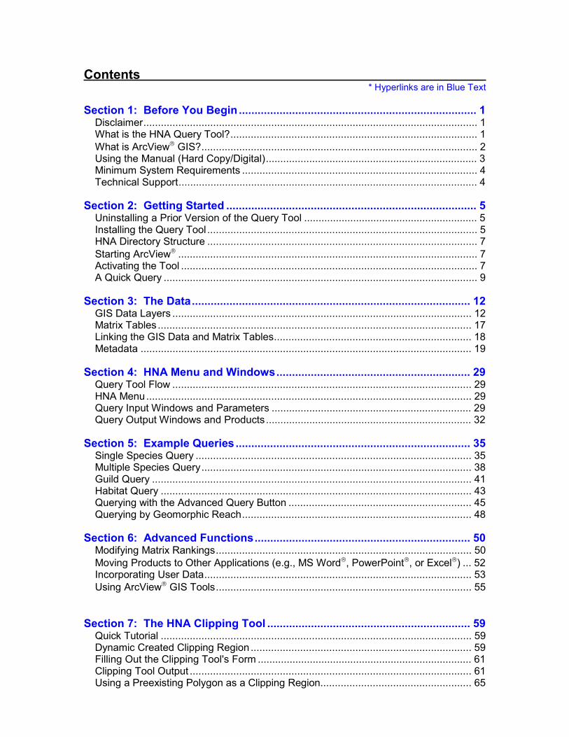
Contents * Hyperlinks are in Blue Text
Section 1: Before You Begin ............................................................................ 1 Disclaimer................................................................................................................... 1 What is the HNA Query Tool?..................................................................................... 1 What is ArcView GIS?............................................................................................... 2 Using the Manual (Hard Copy/Digital)......................................................................... 3 Minimum System Requirements ................................................................................. 4 Technical Support....................................................................................................... 4
Section 2: Getting Started ................................................................................ 5 Uninstalling a Prior Version of the Query Tool ............................................................ 5 Installing the Query Tool ............................................................................................. 5 HNA Directory Structure ............................................................................................. 7 Starting ArcView ....................................................................................................... 7 Activating the Tool ...................................................................................................... 7 A Quick Query ............................................................................................................ 9
Section 3: The Data......................................................................................... 12 GIS Data Layers ....................................................................................................... 12 Matrix Tables ............................................................................................................ 17 Linking the GIS Data and Matrix Tables.................................................................... 18 Metadata .................................................................................................................. 19
Section 4: HNA Menu and Windows.............................................................. 29 Query Tool Flow ....................................................................................................... 29 HNA Menu................................................................................................................ 29 Query Input Windows and Parameters ..................................................................... 29 Query Output Windows and Products....................................................................... 32
Section 5: Example Queries ........................................................................... 35 Single Species Query ............................................................................................... 35 Multiple Species Query............................................................................................. 38 Guild Query .............................................................................................................. 41 Habitat Query ........................................................................................................... 43 Querying with the Advanced Query Button ............................................................... 45 Querying by Geomorphic Reach............................................................................... 48
Section 6: Advanced Functions..................................................................... 50 Modifying Matrix Rankings........................................................................................ 50 Moving Products to Other Applications (e.g., MS Word, PowerPoint, or Excel) ... 52 Incorporating User Data............................................................................................ 53 Using ArcView GIS Tools........................................................................................ 55
Section 7: The HNA Clipping Tool ................................................................. 59 Quick Tutorial ........................................................................................................... 59 Dynamic Created Clipping Region ............................................................................ 59 Filling Out the Clipping Tool's Form .......................................................................... 61 Clipping Tool Output ................................................................................................. 61 Using a Preexisting Polygon as a Clipping Region.................................................... 65
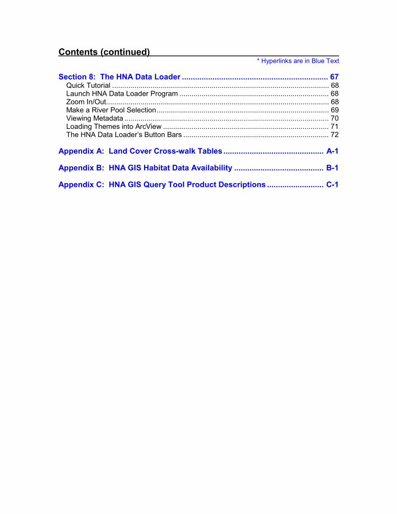
Contents (continued) * Hyperlinks are in Blue Text
Section 8: The HNA Data Loader ................................................................... 67 Quick Tutorial ........................................................................................................... 68 Launch HNA Data Loader Program .......................................................................... 68 Zoom In/Out.............................................................................................................. 68 Make a River Pool Selection..................................................................................... 69 Viewing Metadata ..................................................................................................... 70 Loading Themes into ArcView .................................................................................. 71 The HNA Data Loader’s Button Bars ........................................................................ 72
Appendix A: Land Cover Cross-walk Tables .............................................. A-1
Appendix B: HNA GIS Habitat Data Availability ......................................... B-1
Appendix C: HNA GIS Query Tool Product Descriptions .......................... C-1

Section 1: Before You Begin Disclaimer
W TaMauop
F Ts
The Habitat Needs Assessment (HNA) GIS Query Tool generates products (maps, charts, and tables) about POTENTIAL habitat based solely upon land or aquatic classes. Products are generated regardless of the range of species/guilds in the Upper Mississippi River System (UMRS).
Section 1: Before You Begin
1
hat is the HNA GIS Query Tool?
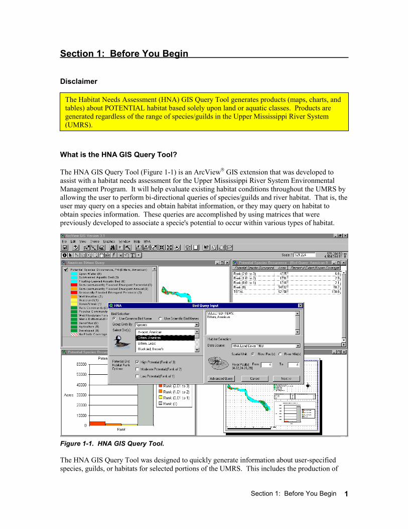
he HNA GIS Query Tool (Figure 1-1) is an ArcView GIS extension that was developed to ssist with a habitat needs assessment for the Upper Mississippi River System Environmental anagement Program. It will help evaluate existing habitat conditions throughout the UMRS by
llowing the user to perform bi-directional queries of species/guilds and river habitat. That is, the ser may query on a species and obtain habitat information, or they may query on habitat to btain species information. These queries are accomplished by using matrices that were reviously developed to associate a specie's potential to occur within various types of habitat.
igure 1-1. HNA GIS Query Tool.
he HNA GIS Query Tool was designed to quickly generate information about user-specified pecies, guilds, or habitats for selected portions of the UMRS. This includes the production of
Section 1: Before You Begin
2
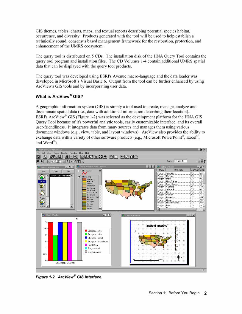
GIS themes, tables, charts, maps, and textual reports describing potential species habitat, occurrence, and diversity. Products generated with the tool will be used to help establish a technically sound, consensus based management framework for the restoration, protection, and enhancement of the UMRS ecosystem. The query tool is distributed on 5 CDs. The installation disk of the HNA Query Tool contains the query tool program and installation files. The CD Volumes 1-4 contain additional UMRS spatial data that can be displayed with the query tool products. The query tool was developed using ESRI's Avenue macro-language and the data loader was developed in Microsoft’s Visual Basic 6. Output from the tool can be further enhanced by using ArcView's GIS tools and by incorporating user data. What is ArcView GIS? A geographic information system (GIS) is simply a tool used to create, manage, analyze and disseminate spatial data (i.e., data with additional information describing their location). ESRI's ArcView GIS (Figure 1-2) was selected as the development platform for the HNA GIS Query Tool because of it's powerful analytic tools, easily customizable interface, and its overall user-friendliness. It integrates data from many sources and manages them using various document windows (e.g., view, table, and layout windows). ArcView also provides the ability to exchange data with a variety of other software products (e.g., Microsoft PowerPoint, Excel, and Word).
Figure 1-2. ArcView GIS interface.
Section 1: Before You Begin
3
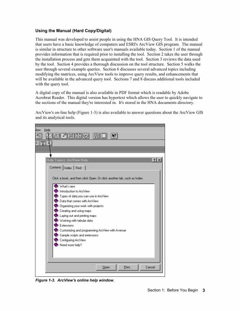
Using the Manual (Hard Copy/Digital) This manual was developed to assist people in using the HNA GIS Query Tool. It is intended that users have a basic knowledge of computers and ESRI's ArcView GIS program. The manual is similar in structure to other software user's manuals available today. Section 1 of the manual provides information that is required prior to installing the tool. Section 2 takes the user through the installation process and gets them acquainted with the tool. Section 3 reviews the data used by the tool. Section 4 provides a thorough discussion on the tool structure. Section 5 walks the user through several example queries. Section 6 discusses several advanced topics including modifying the matrices, using ArcView tools to improve query results, and enhancements that will be available in the advanced query tool. Sections 7 and 8 discuss additional tools included with the query tool. A digital copy of the manual is also available in PDF format which is readable by Adobe Acrobrat Reader. This digital version has hypertext which allows the user to quickly navigate to the sections of the manual they're interested in. It's stored in the HNA documents directory. ArcView's on-line help (Figure 1-3) is also available to answer questions about the ArcView GIS and its analytical tools.
Figure 1-3. ArcView's online help window.
Section 1: Before You Begin
4
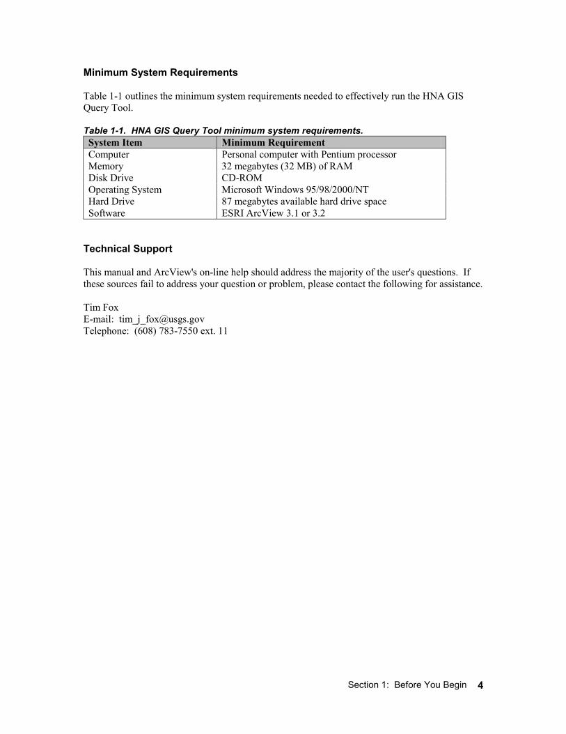
Minimum System Requirements Table 1-1 outlines the minimum system requirements needed to effectively run the HNA GIS Query Tool. Table 1-1. HNA GIS Query Tool minimum system requirements. System Item Minimum Requirement Computer Personal computer with Pentium processor Memory 32 megabytes (32 MB) of RAM Disk Drive CD-ROM Operating System Microsoft Windows 95/98/2000/NT Hard Drive 87 megabytes available hard drive space Software ESRI ArcView 3.1 or 3.2
Technical Support This manual and ArcView's on-line help should address the majority of the user's questions. If these sources fail to address your question or problem, please contact the following for assistance. Tim Fox E-mail: [email protected] Telephone: (608) 783-7550 ext. 11
Section 2: Getting Started
5
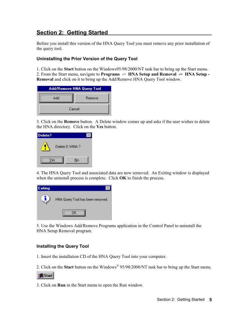
Section 2: Getting Started Before you install this version of the HNA Query Tool you must remove any prior installation of the query tool. Uninstalling the Prior Version of the Query Tool 1. Click on the Start button on the Windows95/98/2000/NT task bar to bring up the Start menu. 2. From the Start menu, navigate to Programs -> HNA Setup and Removal -> HNA Setup - Removal and click on it to bring up the Add/Remove HNA Query Tool window.
3. Click on the Remove button. A Delete window comes up and asks if the user wishes to delete the HNA directory. Click on the Yes button.
4. The HNA Query Tool and associated data are now removed. An Exiting window is displayed when the uninstall process is complete. Click OK to finish the process.
5. Use the Windows Add/Remove Programs application in the Control Panel to uninstall the HNA Setup Removal program. Installing the Query Tool 1. Insert the installation CD of the HNA Query Tool into your computer. 2. Click on the Start button on the Windows 95/98/2000/NT task bar to bring up the Start menu.
3. Click on Run in the Start menu to open the Run window.
Section 2: Getting Started
6
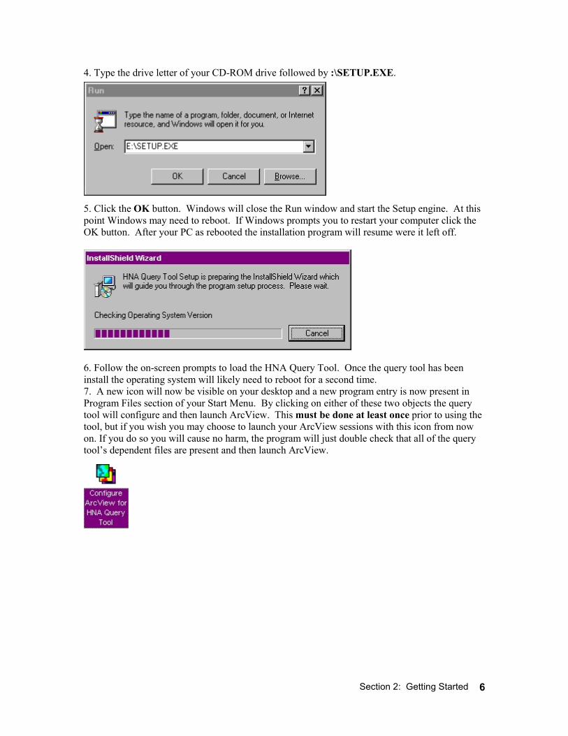
4. Type the drive letter of your CD-ROM drive followed by :\SETUP.EXE.
5. Click the OK button. Windows will close the Run window and start the Setup engine. At this point Windows may need to reboot. If Windows prompts you to restart your computer click the OK button. After your PC as rebooted the installation program will resume were it left off.
6. Follow the on-screen prompts to load the HNA Query Tool. Once the query tool has been install the operating system will likely need to reboot for a second time. 7. A new icon will now be visible on your desktop and a new program entry is now present in Program Files section of your Start Menu. By clicking on either of these two objects the query tool will configure and then launch ArcView. This must be done at least once prior to using the tool, but if you wish you may choose to launch your ArcView sessions with this icon from now on. If you do so you will cause no harm, the program will just double check that all of the query tool’s dependent files are present and then launch ArcView.
Section 2: Getting Started
7
HNA Directory Structure Files used by the query tool are stored on the computer in the HNA folder with the following directory structure.
- ArcView project file of the query tool - Installation files - User's Manual and HREP PDF documents - ArcView extension files - GIS data in ArcView shapefile format - Adobe Acrobat Reader 3.01 (used with the HREP hotlink), HNA Data Loader - Habitat summary tables and species matrices
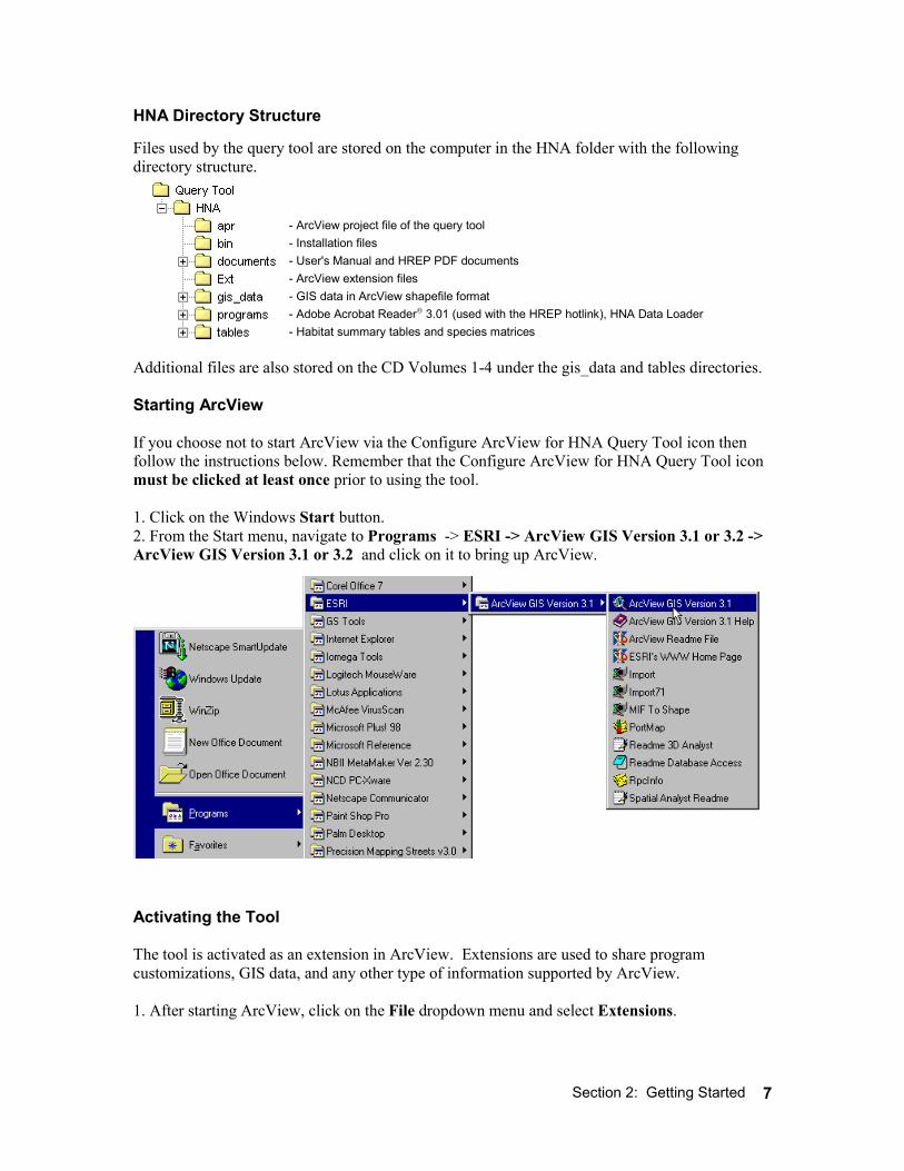
Additional files are also stored on the CD Volumes 1-4 under the gis_data and tables directories. Starting ArcView If you choose not to start ArcView via the Configure ArcView for HNA Query Tool icon then follow the instructions below. Remember that the Configure ArcView for HNA Query Tool icon must be clicked at least once prior to using the tool. 1. Click on the Windows Start button. 2. From the Start menu, navigate to Programs -> ESRI -> ArcView GIS Version 3.1 or 3.2 -> ArcView GIS Version 3.1 or 3.2 and click on it to bring up ArcView.
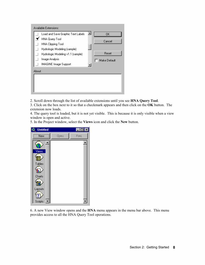
Activating the Tool The tool is activated as an extension in ArcView. Extensions are used to share program customizations, GIS data, and any other type of information supported by ArcView. 1. After starting ArcView, click on the File dropdown menu and select Extensions.
Section 2: Getting Started
8
2. Scroll down through the list of available extensions until you see HNA Query Tool. 3. Click on the box next to it so that a checkmark appears and then click on the OK button. The extension now loads. 4. The query tool is loaded, but it is not yet visible. This is because it is only visible when a view window is open and active. 5. In the Project window, select the Views icon and click the New button.
6. A new View window opens and the HNA menu appears in the menu bar above. This menu provides access to all the HNA Query Tool operations.
Section 2: Getting Started
9
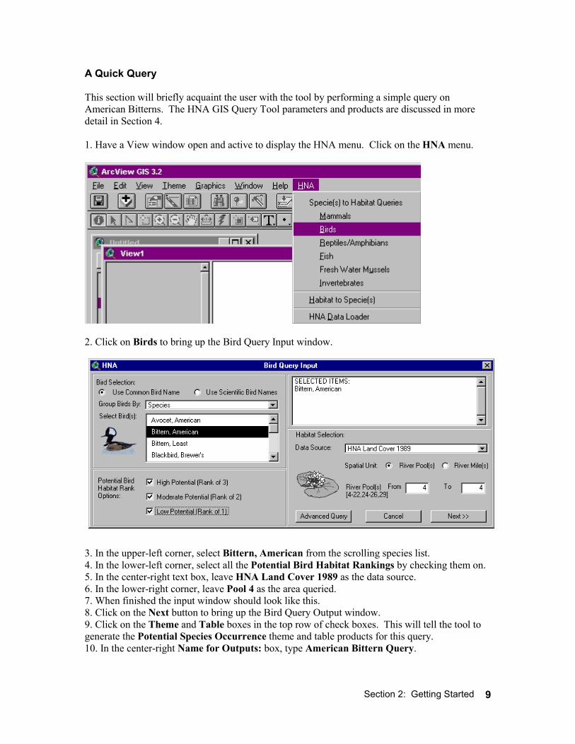
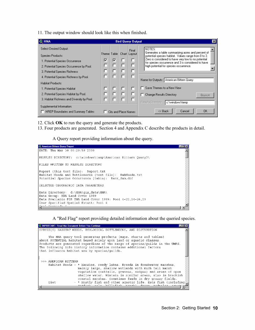
A Quick Query This section will briefly acquaint the user with the tool by performing a simple query on American Bitterns. The HNA GIS Query Tool parameters and products are discussed in more detail in Section 4. 1. Have a View window open and active to display the HNA menu. Click on the HNA menu.
2. Click on Birds to bring up the Bird Query Input window.
3. In the upper-left corner, select Bittern, American from the scrolling species list. 4. In the lower-left corner, select all the Potential Bird Habitat Rankings by checking them on. 5. In the center-right text box, leave HNA Land Cover 1989 as the data source. 6. In the lower-right corner, leave Pool 4 as the area queried. 7. When finished the input window should look like this. 8. Click on the Next button to bring up the Bird Query Output window. 9. Click on the Theme and Table boxes in the top row of check boxes. This will tell the tool to generate the Potential Species Occurrence theme and table products for this query. 10. In the center-right Name for Outputs: box, type American Bittern Query.
Section 2: Getting Started
10
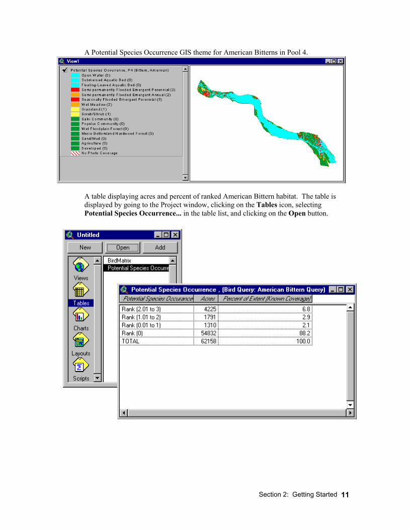
11. The output window should look like this when finished.
12. Click OK to run the query and generate the products. 13. Four products are generated. Section 4 and Appendix C describe the products in detail.
A Query report providing information about the query.
A "Red Flag" report providing detailed information about the queried species.
Section 2: Getting Started
11
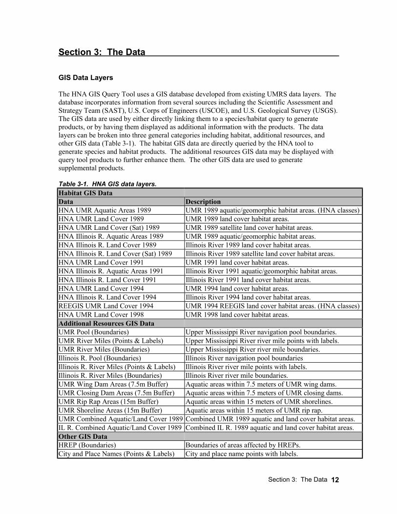
A Potential Species Occurrence GIS theme for American Bitterns in Pool 4.
A table displaying acres and percent of ranked American Bittern habitat. The table is displayed by going to the Project window, clicking on the Tables icon, selecting Potential Species Occurrence... in the table list, and clicking on the Open button.
Section 3: The Data
12
Section 3: The Data GIS Data Layers The HNA GIS Query Tool uses a GIS database developed from existing UMRS data layers. The database incorporates information from several sources including the Scientific Assessment and Strategy Team (SAST), U.S. Corps of Engineers (USCOE), and U.S. Geological Survey (USGS). The GIS data are used by either directly linking them to a species/habitat query to generate products, or by having them displayed as additional information with the products. The data layers can be broken into three general categories including habitat, additional resources, and other GIS data (Table 3-1). The habitat GIS data are directly queried by the HNA tool to generate species and habitat products. The additional resources GIS data may be displayed with query tool products to further enhance them. The other GIS data are used to generate supplemental products. Table 3-1. HNA GIS data layers. Habitat GIS Data Data Description HNA UMR Aquatic Areas 1989 UMR 1989 aquatic/geomorphic habitat areas. (HNA classes) HNA UMR Land Cover 1989 UMR 1989 land cover habitat areas. HNA UMR Land Cover (Sat) 1989 UMR 1989 satellite land cover habitat areas. HNA Illinois R. Aquatic Areas 1989 UMR 1989 aquatic/geomorphic habitat areas. HNA Illinois R. Land Cover 1989 Illinois River 1989 land cover habitat areas. HNA Illinois R. Land Cover (Sat) 1989 Illinois River 1989 satellite land cover habitat areas. HNA UMR Land Cover 1991 UMR 1991 land cover habitat areas. HNA Illinois R. Aquatic Areas 1991 Illinois River 1991 aquatic/geomorphic habitat areas. HNA Illinois R. Land Cover 1991 Illinois River 1991 land cover habitat areas. HNA UMR Land Cover 1994 UMR 1994 land cover habitat areas. HNA Illinois R. Land Cover 1994 Illinois River 1994 land cover habitat areas. REEGIS UMR Land Cover 1994 UMR 1994 REEGIS land cover habitat areas. (HNA classes) HNA UMR Land Cover 1998 UMR 1998 land cover habitat areas. Additional Resources GIS Data UMR Pool (Boundaries) Upper Mississippi River navigation pool boundaries. UMR River Miles (Points & Labels) Upper Mississippi River river mile points with labels. UMR River Miles (Boundaries) Upper Mississippi River river mile boundaries. Illinois R. Pool (Boundaries) Illinois River navigation pool boundaries Illinois R. River Miles (Points & Labels) Illinois River river mile points with labels. Illinois R. River Miles (Boundaries) Illinois River river mile boundaries. UMR Wing Dam Areas (7.5m Buffer) Aquatic areas within 7.5 meters of UMR wing dams. UMR Closing Dam Areas (7.5m Buffer) Aquatic areas within 7.5 meters of UMR closing dams. UMR Rip Rap Areas (15m Buffer) Aquatic areas within 15 meters of UMR shorelines. UMR Shoreline Areas (15m Buffer) Aquatic areas within 15 meters of UMR rip rap. UMR Combined Aquatic/Land Cover 1989 Combined UMR 1989 aquatic and land cover habitat areas. IL R. Combined Aquatic/Land Cover 1989 Combined IL R. 1989 aquatic and land cover habitat areas. Other GIS Data HREP (Boundaries) Boundaries of areas affected by HREPs. City and Place Names (Points & Labels) City and place name points with labels.
Section 3: The Data
13
The habitat GIS data were obtained from the USGS Long Term Resource Monitoring Program (LTRMP) and the USCOE River Engineering and Environmental Geospatial Information System (REEGIS). These existing data sets were reclassified into HNA habitat categories that are ecologically relevant and easily understandable by a wide range of users. The HNA query tool uses two types of habitat data (i.e., aquatic/geomorphic areas and land cover/land use). Tables 3-2 and 3-3 provide information to help characterize the HNA habitat classes. The reclassification process was accomplished using the cross-walk tables displayed in Appendix A. Table 3-2. HNA aquatic/geomorphic classification descriptions. Aquatic/Geomorphic Area Classification Description Main Navigation Channel The designated navigation corridor area of the main channel
marked by channel buoys. In reaches where buoys are not used, the centerline of the navigation channel is defined by lights and daymarks on shore that pilots use to navigate. The navigation channel on most of the UMRS is 91.4m (300 ft) wide in straight reaches and 152.4m (500 ft) feet wide in bends. The navigation channels in the upper pools of the UMRS and tributary waterways are narrower. The navigation channel extends through the locks at each lock and dam. The navigation channel is usually in the main channel, but in some reaches, the navigation channel is located in secondary channels.
Main Channel Border The area between the navigation channel and the river bank. Boundaries of the channel border are the apparent shorelines, the navigation channel buoy line, straight lines across the mouths of secondary and tertiary channels, and along the inundated portions of the natural bank line.
Tailwater Areas downstream of the navigation dams with deep scour holes, high velocity, and turbulent flow. Boundaries of tailwater areas are the navigation dam upstream, the apparent shorelines, and a straight line across the channel 500 meters downstream of the dam.
Secondary Channel Large channels that carry less flow than the main channel. Boundaries are the apparent shorelines, straight lines across the mouths of tertiary channels, and straight lines at the upstream and downstream limits of the apparent shorelines where secondary channels connect with the main channel.
Tertiary Channel Small channels less than 30m wide. The lateral boundaries of tertiary channels are the apparent shorelines. The upstream and downstream limits of tertiary channels are straight lines between the upstream and downstream limits of the apparent shorelines.
Tributary Channel Channels of tributary streams and rivers. The landward boundary is the line where the tributary crosses the study area boundary. The lateral boundaries are the apparent shorelines. The riverward limits of tributary (including distributary) channels is a line drawn across the downstream limits of the apparent shorelines.
Excavated Channel Man-made channels with flowing water.
Section 3: The Data
14
Table 3-2. Continued. Aquatic/Geomorphic Area Classification Description Contiguous Floodplain Lake Distinct lakes formed by fluvial processes or are manmade.
Contiguous means hydraulically connected by surface gravity flow at reference river discharge. For mapping purposes, contiguous means having apparent surface water connection with the rest of the river.
Contiguous Floodplain Shallow Aquatic Area Portions of floodplain inundated by the navigation dams that are not part of any channels or floodplain lakes. Floodplain shallow aquatic areas are shallow areas usually containing a mosaic of open water and emergent vegetation interspersed among islands. The boundaries of these areas are defined by the apparent shorelines and by other aquatic areas. Boundaries of floodplain shallow aquatic areas are often irregular. Where floodplain shallow aquatic areas grade into impounded areas, the boundaries will be lines connecting the downstream parts of islands or peninsulas across the floodplain.
Contiguous Impounded Area Large, mostly open water areas located in the downstream sections of the navigation pools. The downstream boundary of impounded areas are the navigation dam and connecting dikes. Landward boundaries are the apparent shorelines or the boundaries of other aquatic areas. Upstream boundaries are generally with islands and floodplain shallow aquatic areas. Riverward boundaries are channel border areas.
Isolated Floodplain Aquatic Area Floodplain aquatic areas that are not connected to the rest of the river. Isolated means having no hydraulic connection by surface gravity flow at reference river discharge. For mapping purposes, isolated means having no apparent surface water connection with the rest of the river.
Terrestrial Island Terrestrial areas (at reference river discharge) that are not connected to the floodplain.
Contiguous Terrestrial Floodplain Terrestrial floodplain areas (at reference river discharge) that are not protected by flood control levees.
Isolated Terrestrial Floodplain Terrestrial floodplain areas (at reference river discharge) that are protected by flood control levees.
No Photo Coverage UMRS areas without photo coverage.
Habitat Modifiers – wing dam, closing dam, Aquatic areas within 7.5 meters of a wing dam or closing dam.
Habitat Modifiers – shoreline, rip-rap Aquatic areas within 15 meters of shoreline or rip-rap.

Section 3: The Data
15
Table 3-3. HNA land cover classifications with example plant species. Land Cover/Land Use Classification Common Species Open Water None Submersed Aquatic Bed Wild celery, coontail Floating-Leaved Aquatic Bed Lotus, lily (often accompanied by submergents) Semi-permanently Flooded Emergent Annual Wild rice Semi-permanently Flooded Emergent Perennial Cattail, arrowhead, giant burreed, hardstem bulrush Seasonally Flooded Emergent Annual Wild millet, smartweed, beggartick Seasonally Flooded Emergent Perennial Yellow nut-sedge, sedge meadows Wet Meadow Reed canary grass, rice cutgrass, prairie cord-grass Grassland Big bluestem, foxtail, roadside/levee grass Scrub/Shrub Buttonbush, false indigo, swamp privet Salix Community Willow-dominated shrubs Populus Community Cottonwood-dominated floodplain forest Wet Floodplain Forest Silver maple, green ash, black willow Mesic Bottomland Hardwood Forest Oaks, hickories Agriculture Cultivated fields Developed Urban, rural, residential Sand/Mud Exposed sand beaches and mud flats No Photo Coverage Multiple habitat data layers were developed for various years at different data resolutions. Appendix B displays the availability of GIS habitat data used by the query tool. The Xs denote UMRS reaches that are available for query within each data layer. As with any GIS data set, the HNA habitat data layers are linked to attribute tables containing information about their graphic features (i.e., habitat polygons). Tables 3-5 and 3-6 describe field headings used in the land cover/land use and aquatic/geomorphic attribute tables. Table 3-5. HNA land cover attribute fields. Field DescriptionShape ArcView theme feature type. Area Area of polygon feature in square meters. Perimeter Perimeter length of polygon feature in meters. Hna89l8 ArcView theme feature number. Hna89l8 id ArcView theme feature ID. Lcu89b ArcView theme feature number. (pre-river mile) Lcu89b id ArcView theme feature ID. (pre-river mile) Hna lc18 n HNA land cover habitat classification. (number) Hna lc18 d HNA land cover habitat classification. (text) Leveed Located in leveed area. (yes or no) Pool Pool number. River mile River mile number. Acres Area of polygon in acres. Hectares Area of polygon in hectares. Patch acre Area of habitat patch in acres. Patch hect Area of habitat patch in hectares Preference Average Potential Species Occurrence ranking. SP R Species Richness.

Section 3: The Data
16
Table 3-6. HNA aquatic/geomorphic area attribute fields. Field Description Shape ArcView theme feature type. Area Area of polygon feature in square meters. Perimeter Perimeter length of polygon feature in meters. Hna89a8_ ArcView theme feature number. Hna89a8_id ArcView theme feature ID. Aqa89b_ ArcView theme feature number. (pre-river mile) Aqa89b_id ArcView theme feature ID. (pre-river mile) Hna_aqu_n HNA aquatic area habitat classification. (number) Hna_aqu_d HNA aquatic area habitat classification. (text) Leveed Located in leveed area. (yes or no) Shoreline Located in shoreline area. (yes or no) Rip_rap Located in rip rap area. (yes or no) Wing_dam Located in wing dam area. (yes or no) Closing_dam Located in closing dam area. (yes or no) Pool Pool number. River_mile River mile number. Acres Area of polygon in acres. Hectares Area of polygon in hectares. Patch_acre Area of habitat patch in acres. Patch_hect Area of habitat patch in hectares Preference Average Potential Species Occurrence ranking. SP_R Species Richness. The Hna_lc18_d and Hna_aqu_d fields contain the polygon feature's HNA habitat classification. Location and size information are also available for the habitat polygons. Location is classified in the table by pool and river mile. It is also characterized by whether a polygon falls within a leveed area or an aquatic area near shorelines, rip rap, wing dams, or closing dams. The habitat polygon size is available in square meters, acres, and hectares. The Patch_acre and Patch_hect fields refer to the total size of a habitat patch (e.g., area not split by the river mile boundary lines) (Figure 3-1). If a user wishes to query on total habitat area size, they should use the Patch_acre and Patch_hect fields.
Figure 3-1. Habitat area with associated Acre and Patch_acre values.
Section 3: The Data
17
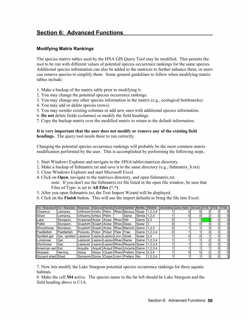
Matrix Tables A series of relational matrix tables were developed to link UMRS species/guilds with habitat areas (Table 3-7). Each row represents a species, and the columns (i.e., fields) display information about the species. Table 3-7. A portion of the HNA fish matrix table. Cn Species2 Cn Species Species Genus Family Guild Habitat Bottle Distrib shoreline wing dam rip-rap C1A C2A C3AChestnut Lamprey, Ichthyom Ichthy Petro Rheo Becaus Spaw 1,2,3,4 1 0 0 2 3 0 Lake Sturgeon, Acipense Acipe Acipe Rheo Silt- Dams 2,3 0 1 1 3 3 3 Pallid Sturgeon, Scaphirh Scaph Acipe Rheo Deep, Spaw 3 0 1 0 3 3 0 Shovelnose Sturgeon, Scaphirh Scaph Acipe Rheo Macroh Same 1,2,3 0 1 1 3 3 3 Paddlefish Paddlefish Polyodo Polyo Polyd Pela Free Dams 1,2,3,4 0 1 1 3 3 3 Spotted gar Gar, spotted Lepisost Lepiso Lepiso Limn Quiet Spaw 2,4 1 0 0 1 3 0 Longnose Gar, Lepisost Lepiso Lepiso Rheo Same Same 1,2,3,4 1 1 1 2 3 3 Shortnose Gar, Lepisost Lepiso Lepiso Rheo Require Spaw 1,2,3,4 1 1 1 2 3 2 American eel Eel, Arguilla Arguill Anguil Rheo Uncerta Dams 1,2,3,4 1 1 1 1 3 2 Skipjack Herring, Alosa Alosa Clupei Rheo Prefers Dams 2,3,4 1 0 0 2 3 0 Gizzard shad Shad, Dorosom Doros Clupei Limn Prefers No 1,2,3,4 1 1 1 3 3 3 The matrix tables contain HNA habitat fields for aquatic/geomorphic areas and land cover/land use. Table 3-8 displays the habitat field headings and what they represent. For example, the field C1A represents Main Navigation Channel aquatic area. Table 3-8. HNA matrix habitat field classifications.
Aquatic/Geomorphic Areas Land Cover/Land Use Field Classification Field Classification C1A Main Navigation Channel C1L Open Water C2A Main Channel Border C2L Submersed Aquatic Bed C3A Tailwater C3L Floating-Leaved Aquatic Bed C4A Secondary Channel C4L Semi-permanently Flooded Emergent Annual C5A Tertiary Channel C5L Semi-permanently Flooded Emergent Perennial C6A Tributary Channel C6L Seasonally Flooded Emergent Annual C7A Excavated Channel C7L Seasonally Flooded Emergent Perennial C8A Contiguous Floodplain Lake C8L Wet Meadow C9A Contiguous Floodplain Shallow Aquatic Area C9L Grassland C10A Contiguous Impounded Area C10L Scrub/Shrub C11A Isolated Floodplain Aquatic Area C11L Salix Community C12A Terrestrial Island C12L Populus Community C13A Contiguous Terrestrial Floodplain C13L Wet Floodplain Forest C14A Isolated Terrestrial Floodplain C14L Mesic Bottomland Hardwood Forest C15A No Photo Coverage C15L Agriculture
C16L Developed C17L Sand/Mud C18L No Photo Coverage
Section 3: The Data
18
The relationship between species/guilds and habitat areas was ranked using a 0 to 3 score. This rank represents the potential for a species/guild to occur within a habitat area: (0 = very low potential, 1 = low potential, 2 = moderate potential, and 3 = high potential to occur within a habitat area). Additional species information (e.g., species/guild common name, distribution, habitat needs, and ecological bottlenecks) is also stored in the matrix tables (Table 3-9). Table 3-9. HNA matrix general and additional bird field descriptions. Gen. Field Description Bird Field Description Cn_Species2 Common species name. Bird _code AOU four letter bird species code. Cn_Species Common species name. Habitat2 Additional habitat field for extended text. Species Genus species name. Diet Preferred diet. Genus Genus name. Diet2 Additional diet field for extended text. Cn_family Comman family name. Status Conservation status. Family Family name. Status2 Additional status field for extended text. Cn_order Common order name. Life Cycle Life cycle stages spent on UMRS. Order Order name. FWS RCP Region 3 FWS resource conservation priorities. Cn_guild Common guild name. PIF S16 Partners in flight strata 16. Guild Guild name. PIF S20 Partners in flight strata 20. Habitat Habitat requirements. PIF S31 Partners in flight strata 31. Bottle Ecological bottlenecks. PIF S32 Partners in flight strata 32. Distrib Distibution of species by UMRS reach. PIF S40 Partners in flight strata 40. Shoreline Potential to occur in shoreline area. 0/1 Wing dam Potential to occur in wing dam area.0/1 Rip-rap Potential to occur in rip-rap area. 0/1 Linking the GIS Data and Matrix Tables The HNA GIS Query Tool operates by linking the species/guild matrix tables to GIS habitat data. This linkage is used to provide potential habitat information about a selected species. Conversely, this linkage is also used to provide species/guild information about specified habitats. After a user selects a species to query on, the tool first searches and selects the species in the matrix table. Then, using the matrix table, it examines the habitat data for the selected species. With this information, the tool then queries the GIS habitat data and generates the selected theme, table, chart, and/or map products. For example, the potential species occurrence theme product was generated for the American Bittern in the previous section. To accomplish this, the tool first queried the bird matrix and selected the American Bittern row of information. It then examined the habitat rankings in this row. Finally, it linked this information to the GIS habitat data and generated a graphic depiction of the potential species occurrence rankings within the habitat areas (Figure 3-2).
Figure 3-2. Potential Species Occurrence GIS theme for American Bitterns in Pool 4.
Section 3: The Data
19
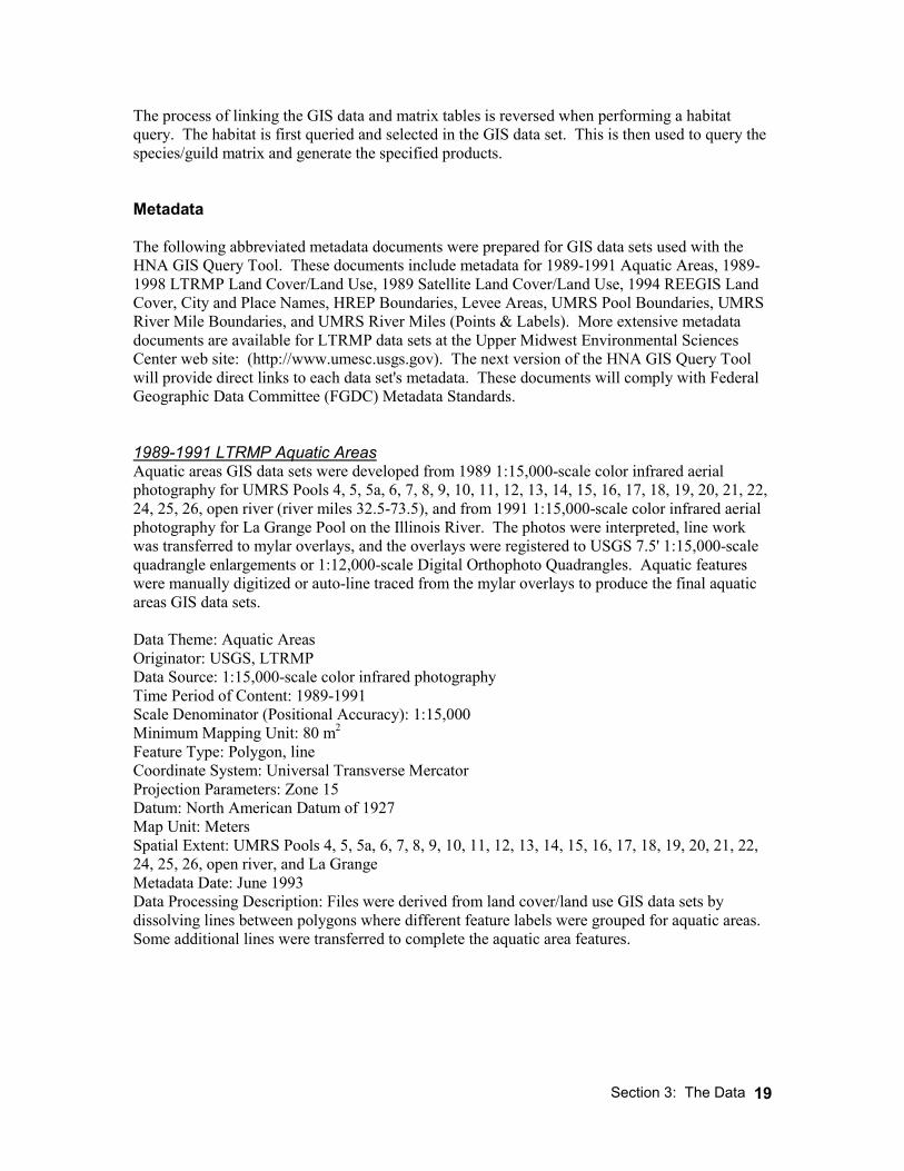
The process of linking the GIS data and matrix tables is reversed when performing a habitat query. The habitat is first queried and selected in the GIS data set. This is then used to query the species/guild matrix and generate the specified products. Metadata The following abbreviated metadata documents were prepared for GIS data sets used with the HNA GIS Query Tool. These documents include metadata for 1989-1991 Aquatic Areas, 1989-1998 LTRMP Land Cover/Land Use, 1989 Satellite Land Cover/Land Use, 1994 REEGIS Land Cover, City and Place Names, HREP Boundaries, Levee Areas, UMRS Pool Boundaries, UMRS River Mile Boundaries, and UMRS River Miles (Points & Labels). More extensive metadata documents are available for LTRMP data sets at the Upper Midwest Environmental Sciences Center web site: (http://www.umesc.usgs.gov). The next version of the HNA GIS Query Tool will provide direct links to each data set's metadata. These documents will comply with Federal Geographic Data Committee (FGDC) Metadata Standards. 1989-1991 LTRMP Aquatic Areas Aquatic areas GIS data sets were developed from 1989 1:15,000-scale color infrared aerial photography for UMRS Pools 4, 5, 5a, 6, 7, 8, 9, 10, 11, 12, 13, 14, 15, 16, 17, 18, 19, 20, 21, 22, 24, 25, 26, open river (river miles 32.5-73.5), and from 1991 1:15,000-scale color infrared aerial photography for La Grange Pool on the Illinois River. The photos were interpreted, line work was transferred to mylar overlays, and the overlays were registered to USGS 7.5' 1:15,000-scale quadrangle enlargements or 1:12,000-scale Digital Orthophoto Quadrangles. Aquatic features were manually digitized or auto-line traced from the mylar overlays to produce the final aquatic areas GIS data sets. Data Theme: Aquatic Areas Originator: USGS, LTRMP Data Source: 1:15,000-scale color infrared photography Time Period of Content: 1989-1991 Scale Denominator (Positional Accuracy): 1:15,000 Minimum Mapping Unit: 80 m2 Feature Type: Polygon, line Coordinate System: Universal Transverse Mercator Projection Parameters: Zone 15 Datum: North American Datum of 1927 Map Unit: Meters Spatial Extent: UMRS Pools 4, 5, 5a, 6, 7, 8, 9, 10, 11, 12, 13, 14, 15, 16, 17, 18, 19, 20, 21, 22, 24, 25, 26, open river, and La Grange Metadata Date: June 1993 Data Processing Description: Files were derived from land cover/land use GIS data sets by dissolving lines between polygons where different feature labels were grouped for aquatic areas. Some additional lines were transferred to complete the aquatic area features.
Section 3: The Data
20
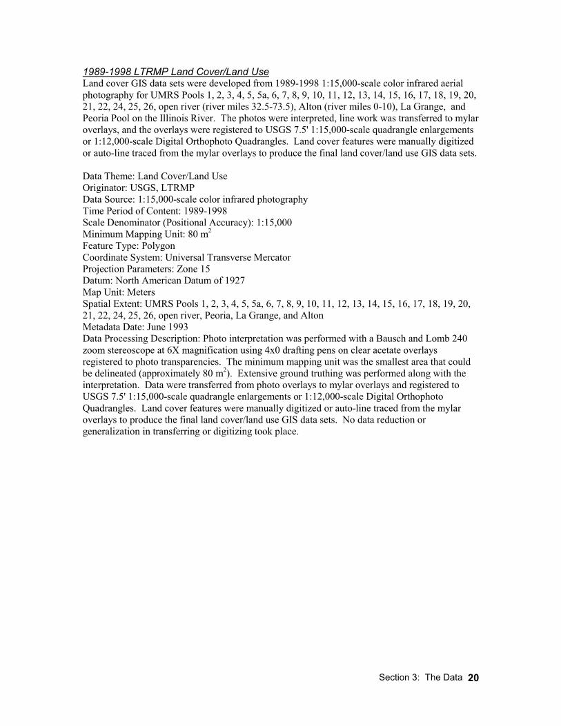
1989-1998 LTRMP Land Cover/Land Use Land cover GIS data sets were developed from 1989-1998 1:15,000-scale color infrared aerial photography for UMRS Pools 1, 2, 3, 4, 5, 5a, 6, 7, 8, 9, 10, 11, 12, 13, 14, 15, 16, 17, 18, 19, 20, 21, 22, 24, 25, 26, open river (river miles 32.5-73.5), Alton (river miles 0-10), La Grange, and Peoria Pool on the Illinois River. The photos were interpreted, line work was transferred to mylar overlays, and the overlays were registered to USGS 7.5' 1:15,000-scale quadrangle enlargements or 1:12,000-scale Digital Orthophoto Quadrangles. Land cover features were manually digitized or auto-line traced from the mylar overlays to produce the final land cover/land use GIS data sets. Data Theme: Land Cover/Land Use Originator: USGS, LTRMP Data Source: 1:15,000-scale color infrared photography Time Period of Content: 1989-1998 Scale Denominator (Positional Accuracy): 1:15,000 Minimum Mapping Unit: 80 m2 Feature Type: Polygon Coordinate System: Universal Transverse Mercator Projection Parameters: Zone 15 Datum: North American Datum of 1927 Map Unit: Meters Spatial Extent: UMRS Pools 1, 2, 3, 4, 5, 5a, 6, 7, 8, 9, 10, 11, 12, 13, 14, 15, 16, 17, 18, 19, 20, 21, 22, 24, 25, 26, open river, Peoria, La Grange, and Alton Metadata Date: June 1993 Data Processing Description: Photo interpretation was performed with a Bausch and Lomb 240 zoom stereoscope at 6X magnification using 4x0 drafting pens on clear acetate overlays registered to photo transparencies. The minimum mapping unit was the smallest area that could be delineated (approximately 80 m2). Extensive ground truthing was performed along with the interpretation. Data were transferred from photo overlays to mylar overlays and registered to USGS 7.5' 1:15,000-scale quadrangle enlargements or 1:12,000-scale Digital Orthophoto Quadrangles. Land cover features were manually digitized or auto-line traced from the mylar overlays to produce the final land cover/land use GIS data sets. No data reduction or generalization in transferring or digitizing took place.
Section 3: The Data
21
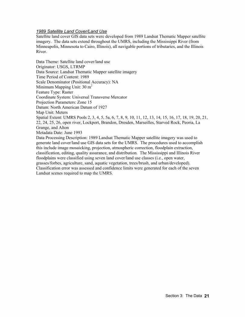
1989 Satellite Land Cover/Land Use Satellite land cover GIS data sets were developed from 1989 Landsat Thematic Mapper satellite imagery. The data sets extend throughout the UMRS, including the Mississippi River (from Minneapolis, Minnesota to Cairo, Illinois), all navigable portions of tributaries, and the Illinois River. Data Theme: Satellite land cover/land use Originator: USGS, LTRMP Data Source: Landsat Thematic Mapper satellite imagery Time Period of Content: 1989 Scale Denominator (Positional Accuracy): NA Minimum Mapping Unit: 30 m2 Feature Type: Raster Coordinate System: Universal Transverse Mercator Projection Parameters: Zone 15 Datum: North American Datum of 1927 Map Unit: Meters Spatial Extent: UMRS Pools 2, 3, 4, 5, 5a, 6, 7, 8, 9, 10, 11, 12, 13, 14, 15, 16, 17, 18, 19, 20, 21, 22, 24, 25, 26, open river, Lockport, Brandon, Dresden, Marseilles, Starved Rock, Peoria, La Grange, and Alton Metadata Date: June 1993 Data Processing Description: 1989 Landsat Thematic Mapper satellite imagery was used to generate land cover/land use GIS data sets for the UMRS. The procedures used to accomplish this include image mosaicking, projection, atmospheric correction, floodplain extraction, classification, editing, quality assurance, and distribution. The Mississippi and Illinois River floodplains were classified using seven land cover/land use classes (i.e., open water, grasses/forbes, agriculture, sand, aquatic vegetation, trees/brush, and urban/developed). Classification error was assessed and confidence limits were generated for each of the seven Landsat scenes required to map the UMRS.
Section 3: The Data
22
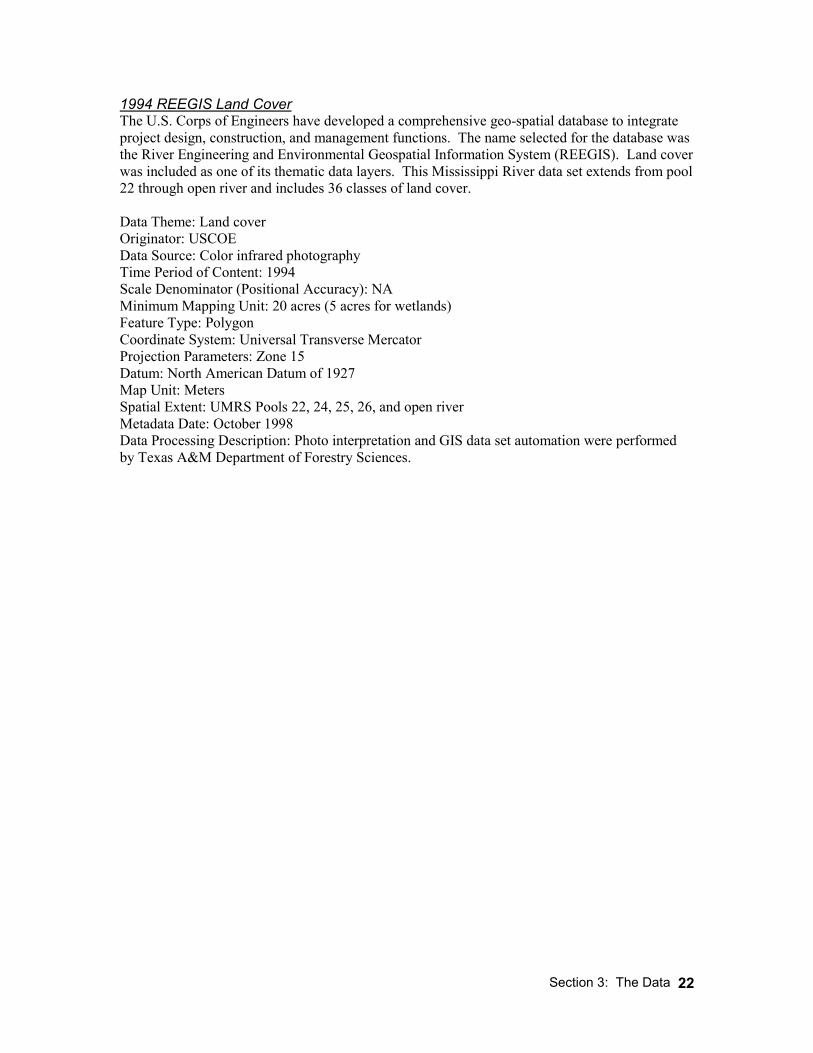
1994 REEGIS Land Cover The U.S. Corps of Engineers have developed a comprehensive geo-spatial database to integrate project design, construction, and management functions. The name selected for the database was the River Engineering and Environmental Geospatial Information System (REEGIS). Land cover was included as one of its thematic data layers. This Mississippi River data set extends from pool 22 through open river and includes 36 classes of land cover. Data Theme: Land cover Originator: USCOE Data Source: Color infrared photography Time Period of Content: 1994 Scale Denominator (Positional Accuracy): NA Minimum Mapping Unit: 20 acres (5 acres for wetlands) Feature Type: Polygon Coordinate System: Universal Transverse Mercator Projection Parameters: Zone 15 Datum: North American Datum of 1927 Map Unit: Meters Spatial Extent: UMRS Pools 22, 24, 25, 26, and open river Metadata Date: October 1998 Data Processing Description: Photo interpretation and GIS data set automation were performed by Texas A&M Department of Forestry Sciences.
Section 3: The Data
23
City and Place Names (from the Geographic Names Information System) The Geographic Names Information System contains name and locative information about almost 2 million physical and cultural features located throughout the United States and its Territories. It was developed by the U.S. Geological Survey in cooperation with the U.S. Board on Geographic Names to promote the standardization of feature names. The first phase is complete for the entire U.S., and entailed the collection of names from Federal sources including large-scale USGS topographic maps, Office of Coast Survey charts, U.S. Forest Service maps and digital data sets distributed by the Federal Communications Commission, the Federal Aviation Administration, and the U.S. Army Corps of Engineers. Data Theme: City and Place Names Originator: USGS Data Source: USGS topographic maps, Office of Coast Survey charts, U.S. Forest Service maps, and digital data sets Time Period of Content: 2000 Scale Denominator (Positional Accuracy): 1:24,000 Minimum Mapping Unit: NA Feature Type: Point Coordinate System: Universal Transverse Mercator Projection Parameters: Zone 15 Datum: North American Datum of 1927 Map Unit: Meters Spatial Extent: On or near the Mississippi and Illinois River Floodplains. Metadata Date: January 1995 Data Processing Description: The Geographic Names Information System was compiled by collecting and editing feature name and location information from the largest-scale USGS topographic maps available. These data were then compared to the records of the U.S. Board on Geographic Names.
Section 3: The Data
24
HREP Boundaries The HREP boundary information represents areas potentially impacted by Habitat Rehabilitation and Enhancement Projects. The boundaries were delineated by scientists and researchers for areas within the UMRS. Data Theme: HREP Boundaries Originator: USGS, LTRMP Data Source: USGS 7.5' 1:24,000-scale topographic maps Time Period of Content: 1997 Scale Denominator (Positional Accuracy): 1:24,000 Minimum Mapping Unit: NA Feature Type: Polygon Coordinate System: Universal Transverse Mercator Projection Parameters: Zone 15 Datum: North American Datum of 1927 Map Unit: Meters Spatial Extent: On or near the Mississippi and Illinois River Floodplains. Metadata Date: NA Data Processing Description: Areas potentially affected by HREPs were delineated by Mississippi River researchers on 1:24,000-scale 7.5' quadrangle base maps. These maps were then digitized and the HREP boundaries were combined into one final GIS data set for the UMRS.
Section 3: The Data
25
Levee Areas On January 10, 1994, the Scientific Assessment and Strategy Team (SAST) joined in the effort to provide scientific advice and assistance to officials responsible for making decisions with respect to the flood recovery in the Upper Mississippi River Basin. A levee area GIS data set was generated as part of this effort to locate and access information about levee status. Data Theme: Levee Areas Originator: Scientific Assessment and Strategy Team (SAST) Data Source: USGS 7.5' 1:24,000-scale topographic maps and USCOE survey records Time Period of Content: 1993 Scale Denominator (Positional Accuracy): 1:24,000 Minimum Mapping Unit: NA Feature Type: Polygon Coordinate System: Universal Transverse Mercator Projection Parameters: Zone 15 Datum: North American Datum of 1927 Map Unit: Meters Spatial Extent: Upper Mississippi and Missouri River Basins Metadata Date: October 1996 Data Processing Description: The data were derived from hand-drawn lines onto USGS 7.5 minute quadrangle maps using U.S. Army Corps of Engineers survey records as a reference. This information was then digitized and attributed using Arc/Info GIS.
The levee data only include areas protected by flood control levees. Areas with other types of levees (e.g., management levees) were not included. Inconsistencies have also been found in the data set with some missing flood control levee areas.
Section 3: The Data
26
UMRS Pool Boundaries (from the Laustrup UMRS Floodplain GIS data set) A UMRS floodplain data set was created to assist with the floodplain/pool extraction of the 1989 satellite land cover/land use. Floodplain and pool boundaries were delineated from toe of bluff to toe of bluff using satellite imagery, USGS 7.5' 1:24,000-scale topographic maps, and 1:15,000-scale aerial photographs. Data Theme: UMRS Pool Boundaries Originator: USGS, LTRMP Data Source: Landsat Thematic Mapper satellite imagery, USGS 7.5' 1:24,000-scale topographic maps, and 1:15,000-scale aerial photographs Time Period of Content: 1989 Scale Denominator (Positional Accuracy): 1:24,000 Minimum Mapping Unit: 30 m2 Feature Type: Polygon Coordinate System: Universal Transverse Mercator Projection Parameters: Zone 15 Datum: North American Datum of 1927 Map Unit: Meters Spatial Extent: UMRS Pools 1, 2, 3, 4, 5, 5a, 6, 7, 8, 9, 10, 11, 12, 13, 14, 15, 16, 17, 18, 19, 20, 21, 22, 24, 25, 26, open river, Lockport, Brandon, Dresden, Marseilles, Starved Rock, Peoria, La Grange, and Alton Metadata Date: June 1993 Data Processing Description: Floodplain and pool areas were delineated by displaying a portion of the Landsat Thematic Mapper satellite imagery at 2X magnification and interactively digitizing the boundaries. Ancillary data in the form of USGS 7.5' 1:24,000-scale topographic maps and 1:15,000-scale aerial photographs were used to help identify the boundary locations.
Section 3: The Data
27
UMRS River Mile Boundaries A river mile boundary data set was recently produced to examine the longitudinal changes in Mississippi River Floodplain structure. The boundaries were generated by intersecting river mile point locations with a lines that were perpendicular to the floodplain. These river mile areas were then attributed with the river mile number that intersected the downstream boundary line (similar to the pool numbering convention). The original data set covered pools 4-26 on the Mississippi River. This was further extended to include the entire Upper Mississippi and Illinois Rivers. Data Theme: UMRS River Mile Boundaries Originator: USGS, LTRMP Data Source: Laustrup UMRS Floodplain and SAST UMRS River Mile data sets Time Period of Content: 1989-1994 Scale Denominator (Positional Accuracy): 1:100,000 Minimum Mapping Unit: NA Feature Type: Polygon Coordinate System: Universal Transverse Mercator Projection Parameters: Zone 15 Datum: North American Datum of 1927 Map Unit: Meters Spatial Extent: UMRS Pools 1, 2, 3, 4, 5, 5a, 6, 7, 8, 9, 10, 11, 12, 13, 14, 15, 16, 17, 18, 19, 20, 21, 22, 24, 25, 26, open river, Lockport, Brandon, Dresden, Marseilles, Starved Rock, Peoria, La Grange, and Alton Metadata Date: March 2000 Data Processing Description: Arc/Info GIS was used to display floodplain boundaries and river mile points. Lines that intersected the river mile points and were perpendicular to the floodplain were added to the floodplain data set. These new river mile areas were then attributed with the river mile number that intersected the downstream boundary line.
Section 3: The Data
28
UMRS River Miles (Points & Labels) On January 10, 1994, the Scientific Assessment and Strategy Team (SAST) joined in the effort to provide scientific advice and assistance to officials responsible for making decisions with respect to the flood recovery in the Upper Mississippi River Basin. A river mile data set was generated as part of this effort to provide river mile markers for the Missouri, Mississippi and Illinois Rivers. It was created from a point coverage provided to the SAST from the Upper Midwest Environmental Sciences Center and ancillary data from the U.S. Army Corps of Engineers. Data Theme: UMRS River Miles Originator: Scientific Assessment and Strategy Team (SAST) Data Source: USGS 1:100,000-scale Digital Line Graphs Time Period of Content: 1994 Scale Denominator (Positional Accuracy): 1:100,000 Minimum Mapping Unit: NA Feature Type: Point Coordinate System: Universal Transverse Mercator Projection Parameters: Zone 15 Datum: North American Datum of 1927 Map Unit: Meters Spatial Extent: Missouri, Mississippi, and Illinois Rivers. Metadata Date: October 1996 Data Processing Description: The SAST acquired the river mile point data from the Upper Midwest Environmental Sciences Center. The point cover was received on floppy and downloaded to the SAST data base. The other files that were received from the Corps of Engineers contained river miles on the Missouri River with one point every tenth of a mile. The data sets from the COE were used to fill in gaps. This revised data base was used for the shifting of points along the Missouri River. Locations of approximately 700 points, mostly along the Missouri, were found to have discrepancies by comparing locations against the 1:100,000 Digital Line Graph line work (up to 2 miles differences). EROS shifted these points to fall at good locations inside the 1:100,000 hydro channel.
Section 4: HNA Menu and Windows
29
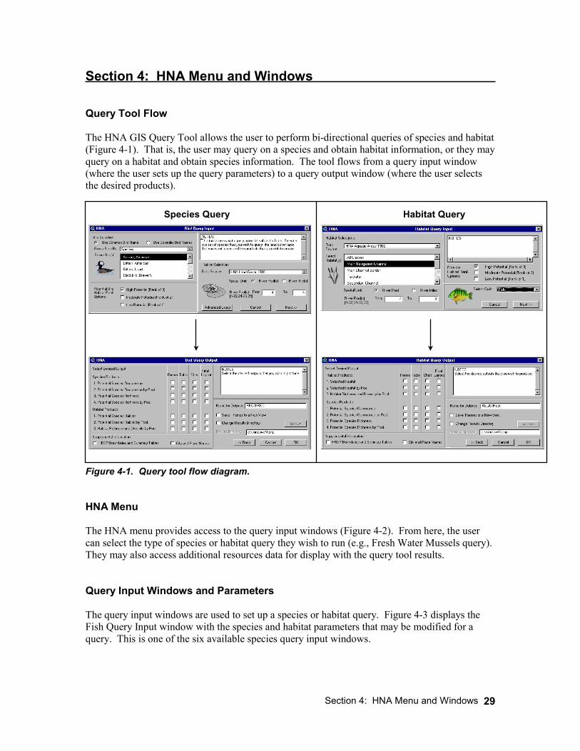
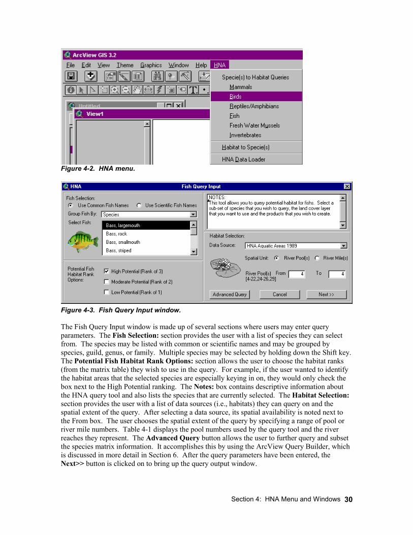
Section 4: HNA Menu and Windows Query Tool Flow The HNA GIS Query Tool allows the user to perform bi-directional queries of species and habitat (Figure 4-1). That is, the user may query on a species and obtain habitat information, or they may query on a habitat and obtain species information. The tool flows from a query input window (where the user sets up the query parameters) to a query output window (where the user selects the desired products).
Figure 4-1. Query tool flow diagram. HNA Menu The HNA menu provides access to the query input windows (Figure 4-2). From here, the user can select the type of species or habitat query they wish to run (e.g., Fresh Water Mussels query). They may also access additional resources data for display with the query tool results. Query Input Windows and Parameters The query input windows are used to set up a species or habitat query. Figure 4-3 displays the Fish Query Input window with the species and habitat parameters that may be modified for a query. This is one of the six available species query input windows.
Species Query Habitat Query
Section 4: HNA Menu and Windows
30
Figure 4-2. HNA menu.
Figure 4-3. Fish Query Input window. The Fish Query Input window is made up of several sections where users may enter query parameters. The Fish Selection: section provides the user with a list of species they can select from. The species may be listed with common or scientific names and may be grouped by species, guild, genus, or family. Multiple species may be selected by holding down the Shift key. The Potential Fish Habitat Rank Options: section allows the user to choose the habitat ranks (from the matrix table) they wish to use in the query. For example, if the user wanted to identify the habitat areas that the selected species are especially keying in on, they would only check the box next to the High Potential ranking. The Notes: box contains descriptive information about the HNA query tool and also lists the species that are currently selected. The Habitat Selection: section provides the user with a list of data sources (i.e., habitats) they can query on and the spatial extent of the query. After selecting a data source, its spatial availability is noted next to the From box. The user chooses the spatial extent of the query by specifying a range of pool or river mile numbers. Table 4-1 displays the pool numbers used by the query tool and the river reaches they represent. The Advanced Query button allows the user to further query and subset the species matrix information. It accomplishes this by using the ArcView Query Builder, which is discussed in more detail in Section 6. After the query parameters have been entered, the Next>> button is clicked on to bring up the query output window.
Section 4: HNA Menu and Windows
31
Table 4-1. Query tool pool numbers and related UMRS river reaches. Upper Mississippi River Upper Mississippi River Pool Number River Reach Pool Number River Reach
1 Pool 1 20 Pool 20 2 Pool 2 21 Pool 21 3 Pool 3 22 Pool 22 4 Pool 4 24 Pool 24 5 Pool 5 25 Pool 25
5.5 Pool 5a 26 Pool 26 6 Pool 6 27 Pool 26 to Kaskaskia River 7 Pool 7 28 Kas. R. to Grand Tower 8 Pool 8 29 Gra. To Ohio River 9 Pool 9 10 Pool 10 Illinois River 11 Pool 11 Pool Number River Reach 12 Pool 12 40 Lockport Pool 13 Pool 13 41 Brandon Pool 14 Pool 14 42 Dresden Pool 15 Pool 15 43 Marseilles Pool 16 Pool 16 44 Starved Rock Pool 17 Pool 17 45 Peoria Pool 18 Pool 18 46 La Grange Pool 19 Pool 19 47 Alton Pool
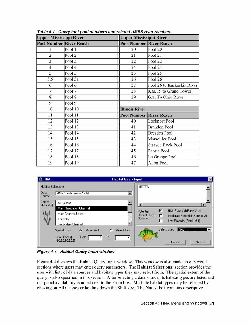
Figure 4-4. Habitat Query Input window. Figure 4-4 displays the Habitat Query Input window. This window is also made up of several sections where users may enter query parameters. The Habitat Selections: section provides the user with lists of data sources and habitats types they may select from. The spatial extent of the query is also specified in this section. After selecting a data source, its habitat types are listed and its spatial availability is noted next to the From box. Multiple habitat types may be selected by clicking on All Classes or holding down the Shift key. The Notes: box contains descriptive

Section 4: HNA Menu and Windows
32
information about the HNA query tool and also lists the habitat types that are selected. The Potential Habitat Rank Options: section allows the user to select the habitat ranks (from the matrix) they wish to use in the query. The Select Guild: section provides a list of the available matrix tables. The matrix table is used in the query to obtain species information related to the selected habitat types and rankings. After the query parameters have been entered, the Next>> button is clicked on to bring up the query output window. Query Output Windows and Products The desired products are selected in query output windows. Figure 4-5 displays the Fish Query Output window with the available product type and format choices.
Figure 4-5. Fish Query Output window. The Fish Query Output window is made up of several sections used to define the desired products. The Notes: box displays descriptive information about the products as their check boxes are clicked on. The Select Desired Output: section provides the user with choices of the type and format of query tool products. Four types of species products and three types of habitat products are available (Table 4-2). They may be produced in several formats including GIS themes, tables, charts, and final layouts (i.e., maps). Graphic examples of the products, with thorough descriptions, are displayed in Appendix C. The Supplemental Information: section is used to generate HREP boundaries (with summary tables) and city and place names in the queried area. In the Name of Outputs: section, the user enters a name that will be displayed with the output (e.g., Largemouth Bass Query) and specifies whether they want to save the products to a new view and/or directory. The Browse button is used to specify the directory where products will be stored. The <<Back button will send the user back to the query input window. Clicking on the OK button will run the query and generate the selected products.
Section 4: HNA Menu and Windows
33
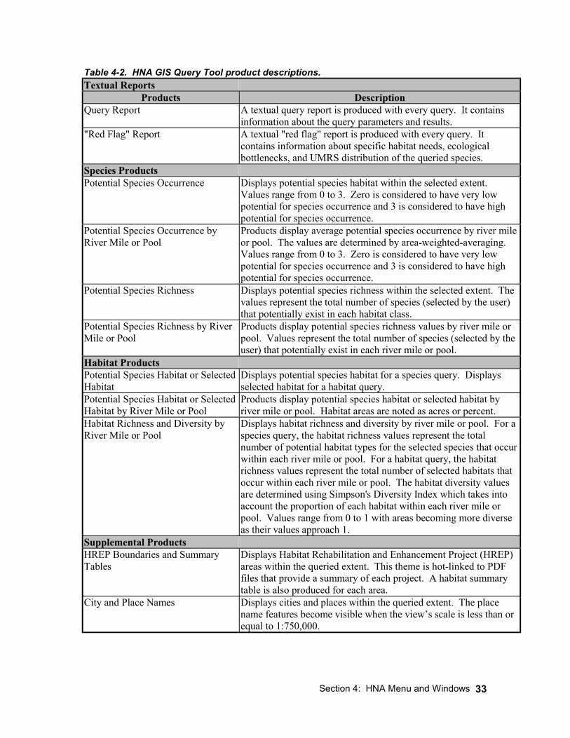
Table 4-2. HNA GIS Query Tool product descriptions. Textual Reports
Products Description Query Report A textual query report is produced with every query. It contains
information about the query parameters and results. "Red Flag" Report A textual "red flag" report is produced with every query. It
contains information about specific habitat needs, ecological bottlenecks, and UMRS distribution of the queried species.
Species Products Potential Species Occurrence Displays potential species habitat within the selected extent.
Values range from 0 to 3. Zero is considered to have very low potential for species occurrence and 3 is considered to have high potential for species occurrence.
Potential Species Occurrence by River Mile or Pool
Products display average potential species occurrence by river mile or pool. The values are determined by area-weighted-averaging. Values range from 0 to 3. Zero is considered to have very low potential for species occurrence and 3 is considered to have high potential for species occurrence.
Potential Species Richness Displays potential species richness within the selected extent. The values represent the total number of species (selected by the user) that potentially exist in each habitat class.
Potential Species Richness by River Mile or Pool
Products display potential species richness values by river mile or pool. Values represent the total number of species (selected by the user) that potentially exist in each river mile or pool.
Habitat Products Potential Species Habitat or Selected Habitat
Displays potential species habitat for a species query. Displays selected habitat for a habitat query.
Potential Species Habitat or Selected Habitat by River Mile or Pool
Products display potential species habitat or selected habitat by river mile or pool. Habitat areas are noted as acres or percent.
Habitat Richness and Diversity by River Mile or Pool
Displays habitat richness and diversity by river mile or pool. For a species query, the habitat richness values represent the total number of potential habitat types for the selected species that occur within each river mile or pool. For a habitat query, the habitat richness values represent the total number of selected habitats that occur within each river mile or pool. The habitat diversity values are determined using Simpson's Diversity Index which takes into account the proportion of each habitat within each river mile or pool. Values range from 0 to 1 with areas becoming more diverse as their values approach 1.
Supplemental Products HREP Boundaries and Summary Tables
Displays Habitat Rehabilitation and Enhancement Project (HREP) areas within the queried extent. This theme is hot-linked to PDF files that provide a summary of each project. A habitat summary table is also produced for each area.
City and Place Names Displays cities and places within the queried extent. The place name features become visible when the view’s scale is less than or equal to 1:750,000.
Section 4: HNA Menu and Windows
34
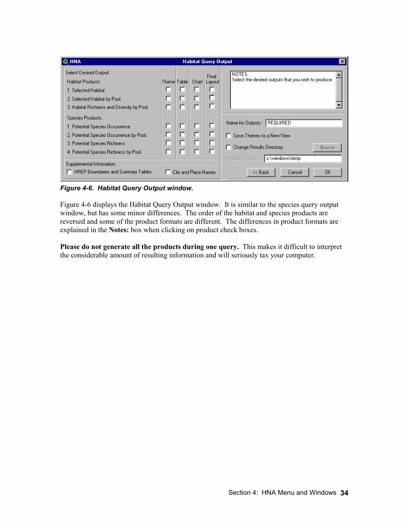
Figure 4-6. Habitat Query Output window. Figure 4-6 displays the Habitat Query Output window. It is similar to the species query output window, but has some minor differences. The order of the habitat and species products are reversed and some of the product formats are different. The differences in product formats are explained in the Notes: box when clicking on product check boxes. Please do not generate all the products during one query. This makes it difficult to interpret the considerable amount of resulting information and will seriously tax your computer.
Section 5: Example Queries
35
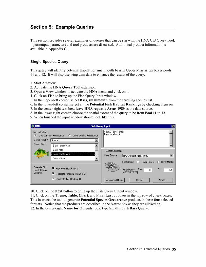
Section 5: Example Queries This section provides several examples of queries that can be run with the HNA GIS Query Tool. Input/output parameters and tool products are discussed. Additional product information is available in Appendix C. Single Species Query This query will identify potential habitat for smallmouth bass in Upper Mississippi River pools 11 and 12. It will also use wing dam data to enhance the results of the query. 1. Start ArcView. 2. Activate the HNA Query Tool extension. 3. Open a View window to activate the HNA menu and click on it. 4. Click on Fish to bring up the Fish Query Input window. 5. In the upper-left corner, select Bass, smallmouth from the scrolling species list. 6. In the lower-left corner, select all the Potential Fish Habitat Rankings by checking them on. 7. In the center-right text box, leave HNA Aquatic Areas 1989 as the data source. 8. In the lower-right corner, choose the spatial extent of the query to be from Pool 11 to 12. 9. When finished the input window should look like this.
10. Click on the Next button to bring up the Fish Query Output window. 11. Click on the Theme, Table, Chart, and Final Layout boxes in the top row of check boxes. This instructs the tool to generate Potential Species Occurrence products in these four selected formats. Notice that the products are described in the Notes: box as they are clicked on. 12. In the center-right Name for Outputs: box, type Smallmouth Bass Query.
Section 5: Example Queries
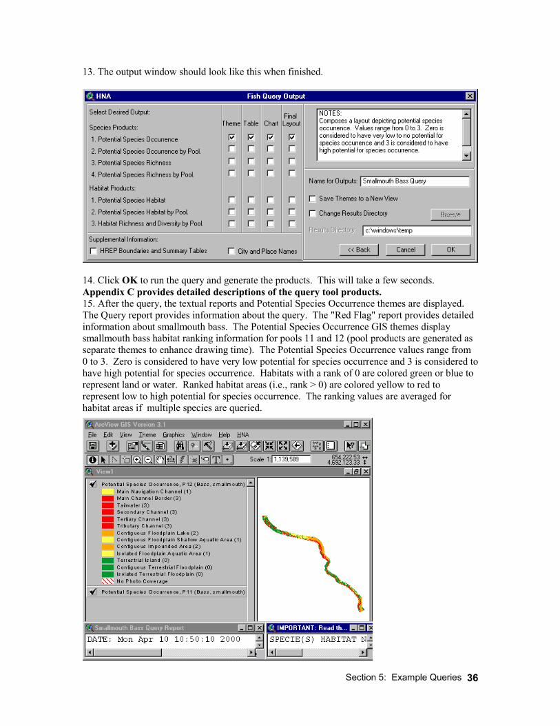
36
13. The output window should look like this when finished.
14. Click OK to run the query and generate the products. This will take a few seconds. Appendix C provides detailed descriptions of the query tool products. 15. After the query, the textual reports and Potential Species Occurrence themes are displayed. The Query report provides information about the query. The "Red Flag" report provides detailed information about smallmouth bass. The Potential Species Occurrence GIS themes display smallmouth bass habitat ranking information for pools 11 and 12 (pool products are generated as separate themes to enhance drawing time). The Potential Species Occurrence values range from 0 to 3. Zero is considered to have very low potential for species occurrence and 3 is considered to have high potential for species occurrence. Habitats with a rank of 0 are colored green or blue to represent land or water. Ranked habitat areas (i.e., rank > 0) are colored yellow to red to represent low to high potential for species occurrence. The ranking values are averaged for habitat areas if multiple species are queried.
Section 5: Example Queries
37
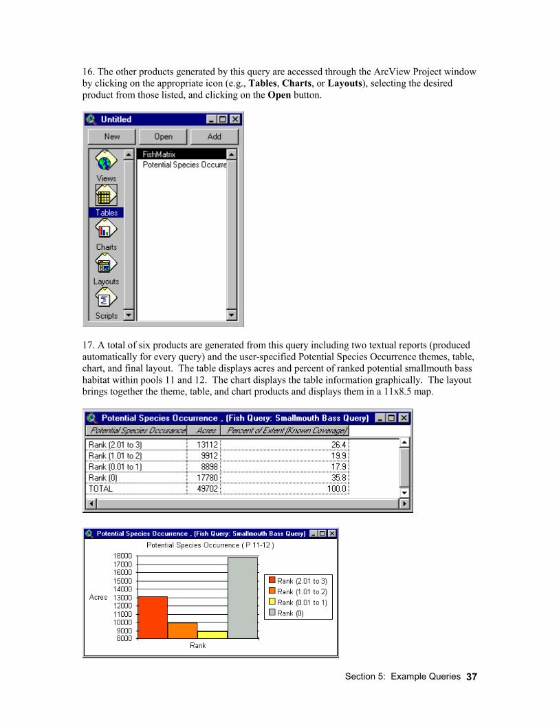
16. The other products generated by this query are accessed through the ArcView Project window by clicking on the appropriate icon (e.g., Tables, Charts, or Layouts), selecting the desired product from those listed, and clicking on the Open button.
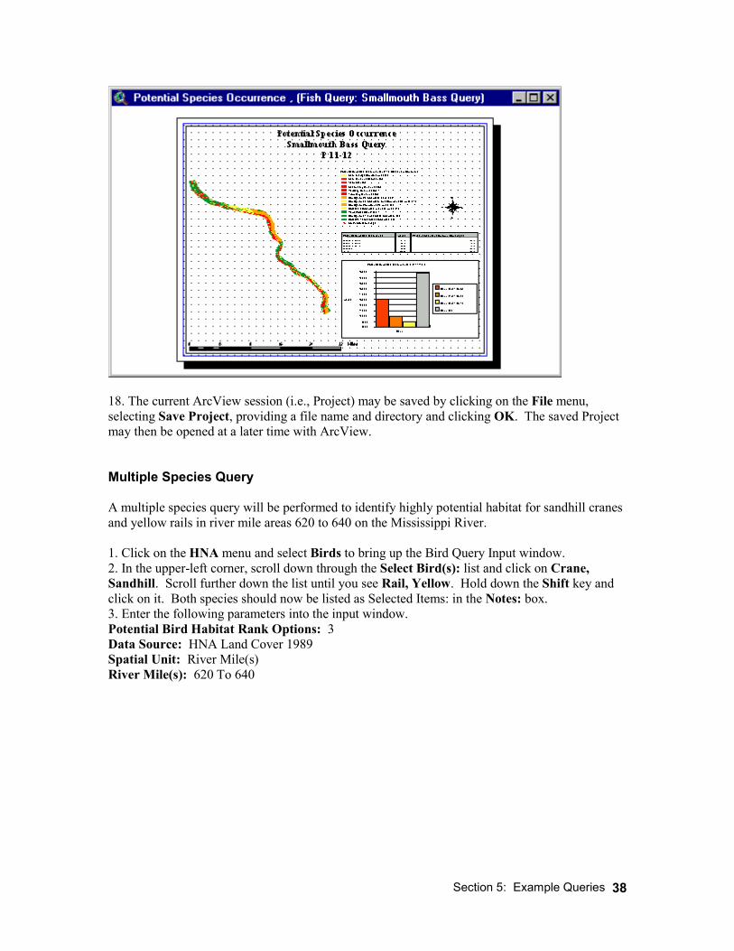
17. A total of six products are generated from this query including two textual reports (produced automatically for every query) and the user-specified Potential Species Occurrence themes, table, chart, and final layout. The table displays acres and percent of ranked potential smallmouth bass habitat within pools 11 and 12. The chart displays the table information graphically. The layout brings together the theme, table, and chart products and displays them in a 11x8.5 map.
Section 5: Example Queries
38
18. The current ArcView session (i.e., Project) may be saved by clicking on the File menu, selecting Save Project, providing a file name and directory and clicking OK. The saved Project may then be opened at a later time with ArcView. Multiple Species Query A multiple species query will be performed to identify highly potential habitat for sandhill cranes and yellow rails in river mile areas 620 to 640 on the Mississippi River. 1. Click on the HNA menu and select Birds to bring up the Bird Query Input window. 2. In the upper-left corner, scroll down through the Select Bird(s): list and click on Crane, Sandhill. Scroll further down the list until you see Rail, Yellow. Hold down the Shift key and click on it. Both species should now be listed as Selected Items: in the Notes: box. 3. Enter the following parameters into the input window. Potential Bird Habitat Rank Options: 3 Data Source: HNA Land Cover 1989 Spatial Unit: River Mile(s) River Mile(s): 620 To 640

Section 5: Example Queries
39
4. When finished, the input window should look like this.
5. Click on the Next button to bring up the Bird Query Output window. The Xs denote the chart products that can't be generated for the current query because there are too many x-axis units. Enter the following parameters. Potential Species Habitat: Theme, Table Supplemental Information: City and Place Names Name for Outputs: Crane and Rail Query Save Themes to a New View: check this box 6. The Output window should look like this when finished.
7. Click OK to run the query and generate the products.
Section 5: Example Queries
40
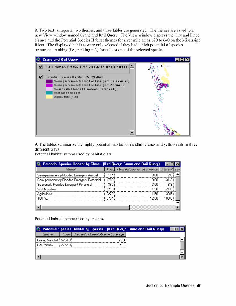
8. Two textual reports, two themes, and three tables are generated. The themes are saved to a new View window named Crane and Rail Query. The View window displays the City and Place Names and the Potential Species Habitat themes for river mile areas 620 to 640 on the Mississippi River. The displayed habitats were only selected if they had a high potential of species occurrence ranking (i.e., ranking = 3) for at least one of the selected species.
9. The tables summarize the highly potential habitat for sandhill cranes and yellow rails in three different ways. Potential habitat summarized by habitat class.
Potential habitat summarized by species.
Section 5: Example Queries
41
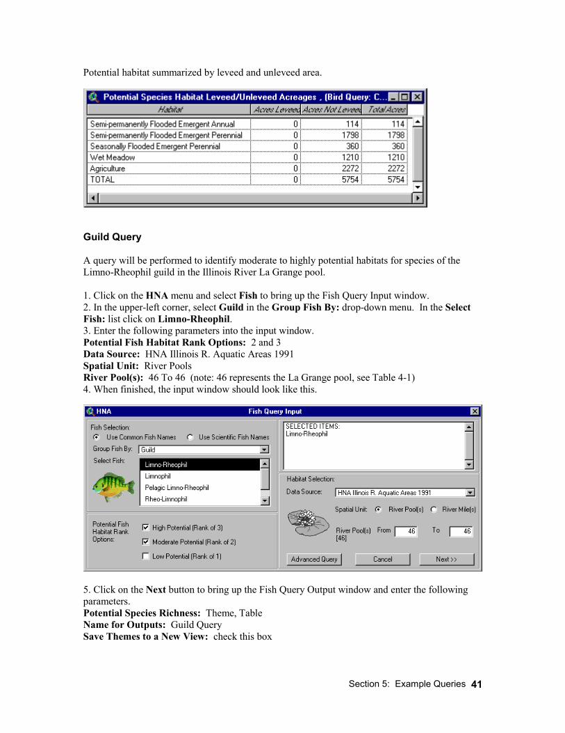
Potential habitat summarized by leveed and unleveed area.
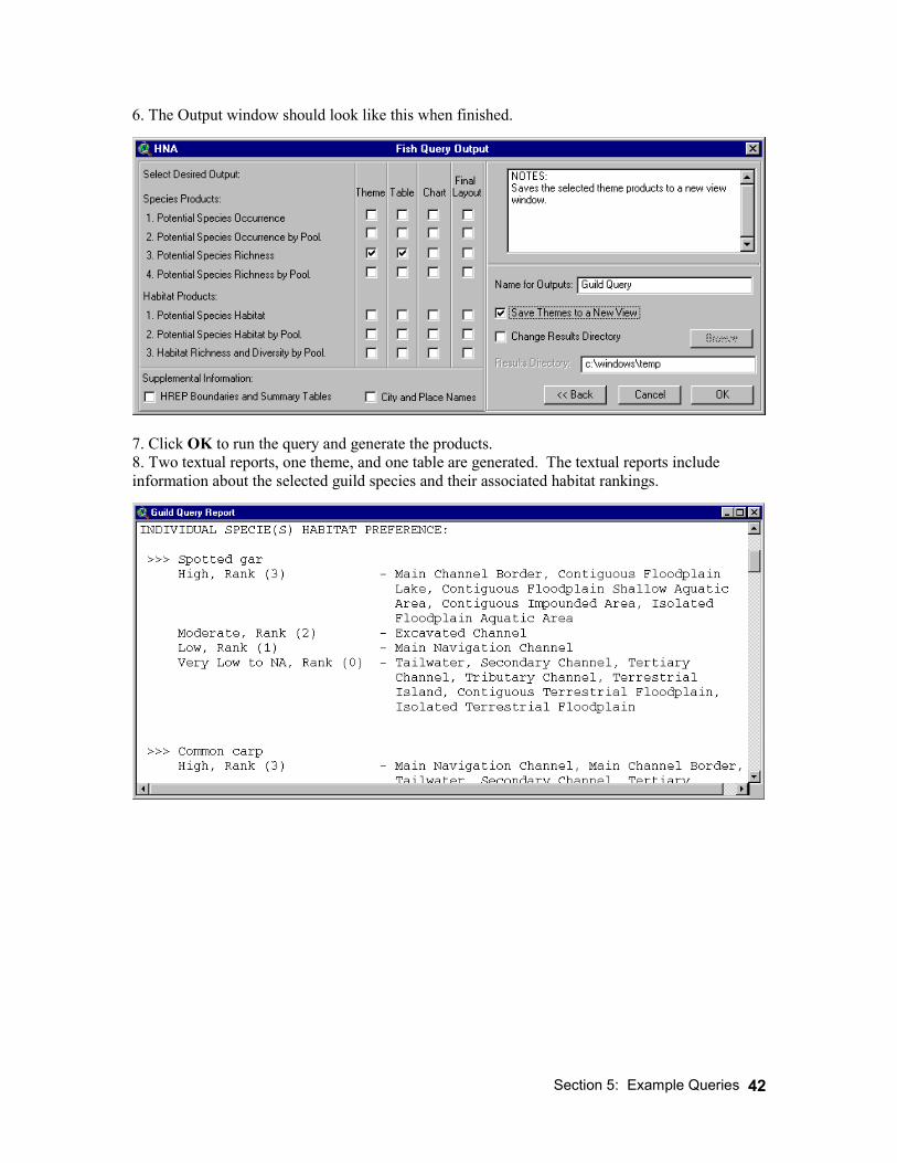
Guild Query A query will be performed to identify moderate to highly potential habitats for species of the Limno-Rheophil guild in the Illinois River La Grange pool. 1. Click on the HNA menu and select Fish to bring up the Fish Query Input window. 2. In the upper-left corner, select Guild in the Group Fish By: drop-down menu. In the Select Fish: list click on Limno-Rheophil. 3. Enter the following parameters into the input window. Potential Fish Habitat Rank Options: 2 and 3 Data Source: HNA Illinois R. Aquatic Areas 1991 Spatial Unit: River Pools River Pool(s): 46 To 46 (note: 46 represents the La Grange pool, see Table 4-1) 4. When finished, the input window should look like this.
5. Click on the Next button to bring up the Fish Query Output window and enter the following parameters. Potential Species Richness: Theme, Table Name for Outputs: Guild Query Save Themes to a New View: check this box
Section 5: Example Queries
42
6. The Output window should look like this when finished.
7. Click OK to run the query and generate the products. 8. Two textual reports, one theme, and one table are generated. The textual reports include information about the selected guild species and their associated habitat rankings.
Section 5: Example Queries
43
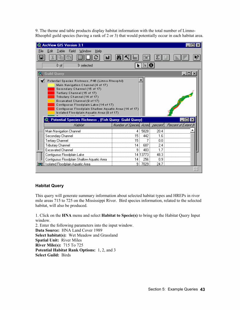
9. The theme and table products display habitat information with the total number of Limno-Rheophil guild species (having a rank of 2 or 3) that would potentially occur in each habitat area.
Habitat Query This query will generate summary information about selected habitat types and HREPs in river mile areas 715 to 725 on the Mississippi River. Bird species information, related to the selected habitat, will also be produced. 1. Click on the HNA menu and select Habitat to Specie(s) to bring up the Habitat Query Input window. 2. Enter the following parameters into the input window. Data Source: HNA Land Cover 1989 Select habitat(s): Wet Meadow and Grassland Spatial Unit: River Miles River Mile(s): 715 To 725 Potential Habitat Rank Options: 1, 2, and 3 Select Guild: Birds
Section 5: Example Queries
44
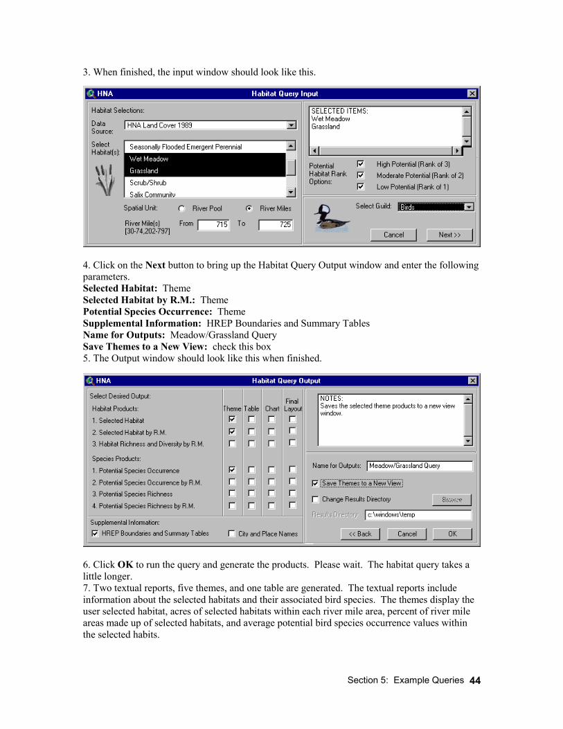
3. When finished, the input window should look like this.
4. Click on the Next button to bring up the Habitat Query Output window and enter the following parameters. Selected Habitat: Theme Selected Habitat by R.M.: Theme Potential Species Occurrence: Theme Supplemental Information: HREP Boundaries and Summary Tables Name for Outputs: Meadow/Grassland Query Save Themes to a New View: check this box 5. The Output window should look like this when finished.
6. Click OK to run the query and generate the products. Please wait. The habitat query takes a little longer. 7. Two textual reports, five themes, and one table are generated. The textual reports include information about the selected habitats and their associated bird species. The themes display the user selected habitat, acres of selected habitats within each river mile area, percent of river mile areas made up of selected habitats, and average potential bird species occurrence values within the selected habits.
Section 5: Example Queries
45
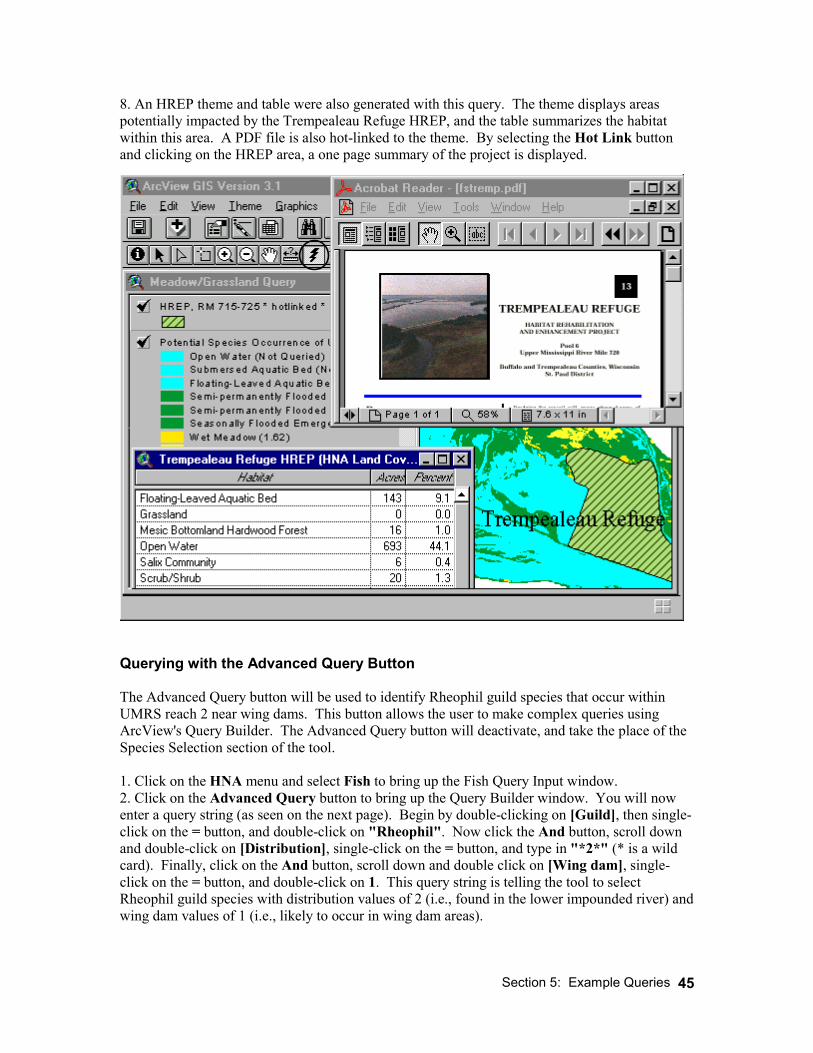
8. An HREP theme and table were also generated with this query. The theme displays areas potentially impacted by the Trempealeau Refuge HREP, and the table summarizes the habitat within this area. A PDF file is also hot-linked to the theme. By selecting the Hot Link button and clicking on the HREP area, a one page summary of the project is displayed.
Querying with the Advanced Query Button The Advanced Query button will be used to identify Rheophil guild species that occur within UMRS reach 2 near wing dams. This button allows the user to make complex queries using ArcView's Query Builder. The Advanced Query button will deactivate, and take the place of the Species Selection section of the tool. 1. Click on the HNA menu and select Fish to bring up the Fish Query Input window. 2. Click on the Advanced Query button to bring up the Query Builder window. You will now enter a query string (as seen on the next page). Begin by double-clicking on [Guild], then single-click on the = button, and double-click on "Rheophil". Now click the And button, scroll down and double-click on [Distribution], single-click on the = button, and type in "*2*" (* is a wild card). Finally, click on the And button, scroll down and double click on [Wing dam], single-click on the = button, and double-click on 1. This query string is telling the tool to select Rheophil guild species with distribution values of 2 (i.e., found in the lower impounded river) and wing dam values of 1 (i.e., likely to occur in wing dam areas).

Section 5: Example Queries
46
Distribution refers to the Upper Mississippi River System area that the species occurs in: (1 = upper impounded, pools 1-13; 2 = lower impounded, pools 14-26; 3 = open river, below pool 26 to the Ohio River confluence; 4 = Illinois river). Wing dam, rip-rap, and shoreline areas are scored 0 or 1. A value of 1 indicates that the species is likely to occur in this type of area. 3. The Query Builder window should look like this when finished.
4. Click the OK button to be brought back to the Fish Query Input window.
note: The advanced query string is now displayed in the notes box. 5. Enter the following parameters into the input window. Potential Fish Habitat Rank Options: 1,2, and 3 Data Source: HNA Aquatic Areas 1989 Spatial Unit: River Pools River Pool(s): 26 To 26 6. When finished, the input window should look like this.
Section 5: Example Queries
47
7. Click on the Next button to bring up the Fish Query Output window and enter the following parameters. Potential Species Richness: Theme, Table Name for Outputs: Advanced Rheophil Query Save Themes to a New View: check this box 8. The Output window should look like this when finished.
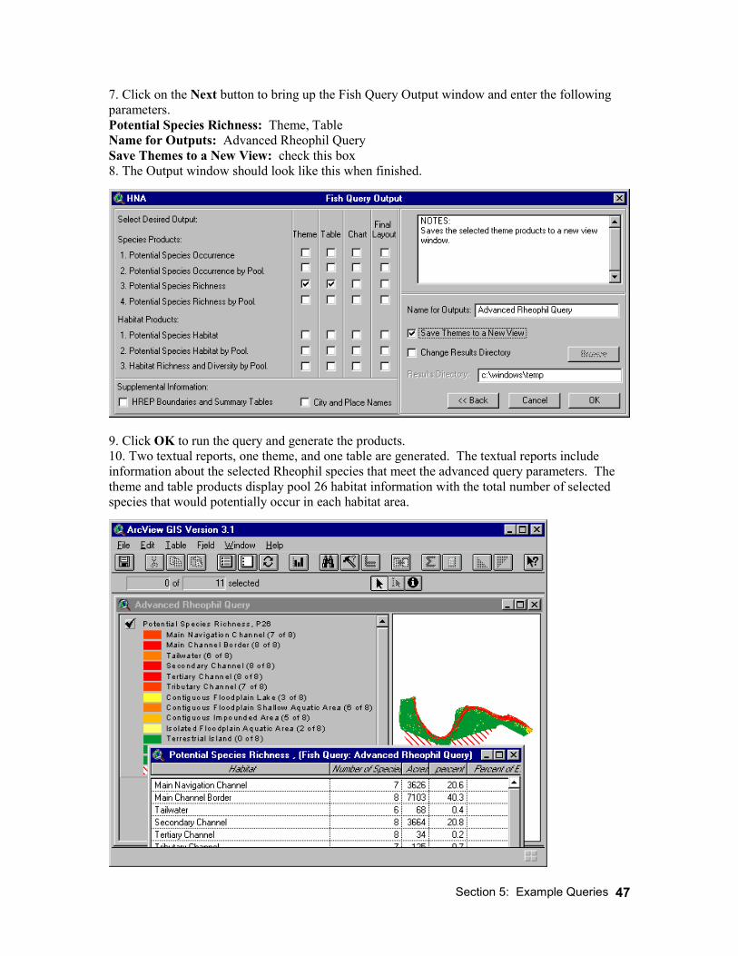
9. Click OK to run the query and generate the products. 10. Two textual reports, one theme, and one table are generated. The textual reports include information about the selected Rheophil species that meet the advanced query parameters. The theme and table products display pool 26 habitat information with the total number of selected species that would potentially occur in each habitat area.
Section 5: Example Queries
48
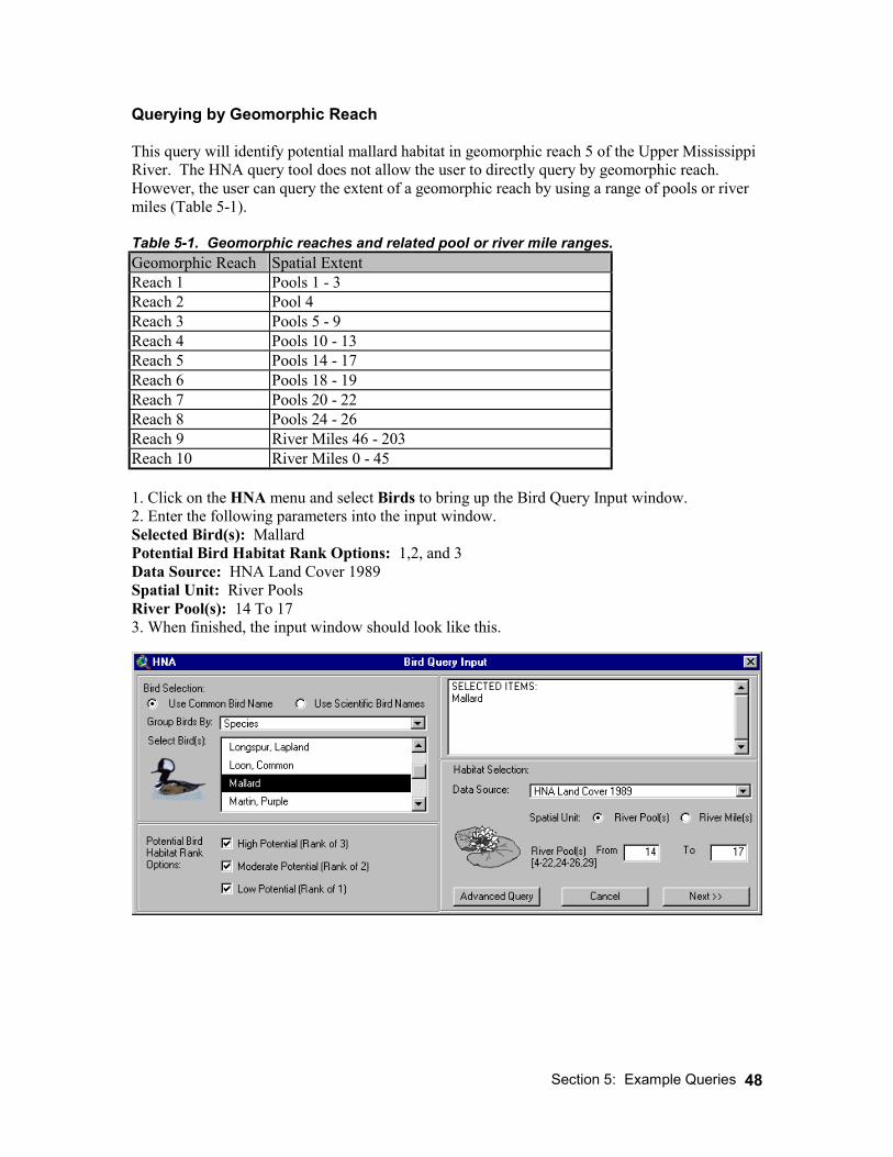
Querying by Geomorphic Reach This query will identify potential mallard habitat in geomorphic reach 5 of the Upper Mississippi River. The HNA query tool does not allow the user to directly query by geomorphic reach. However, the user can query the extent of a geomorphic reach by using a range of pools or river miles (Table 5-1). Table 5-1. Geomorphic reaches and related pool or river mile ranges. Geomorphic Reach Spatial Extent Reach 1 Pools 1 - 3 Reach 2 Pool 4 Reach 3 Pools 5 - 9 Reach 4 Pools 10 - 13 Reach 5 Pools 14 - 17 Reach 6 Pools 18 - 19 Reach 7 Pools 20 - 22 Reach 8 Pools 24 - 26 Reach 9 River Miles 46 - 203 Reach 10 River Miles 0 - 45 1. Click on the HNA menu and select Birds to bring up the Bird Query Input window. 2. Enter the following parameters into the input window. Selected Bird(s): Mallard Potential Bird Habitat Rank Options: 1,2, and 3 Data Source: HNA Land Cover 1989 Spatial Unit: River Pools River Pool(s): 14 To 17 3. When finished, the input window should look like this.
Section 5: Example Queries
49
4. Click on the Next button to bring up the Bird Query Output window and enter the following parameters. Potential Species Occurrence by Pool: Theme, Table Habitat Richness and Diversity by Pool: Theme, Table Name for Outputs: Mallard/Geo. Reach 5 Query Save Themes to a New View: check this box 5. The Output window should look like this when finished.
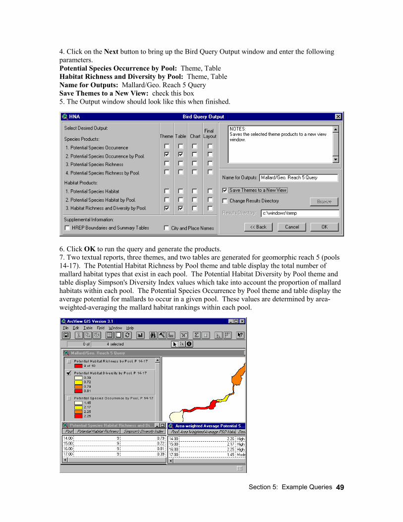
6. Click OK to run the query and generate the products. 7. Two textual reports, three themes, and two tables are generated for geomorphic reach 5 (pools 14-17). The Potential Habitat Richness by Pool theme and table display the total number of mallard habitat types that exist in each pool. The Potential Habitat Diversity by Pool theme and table display Simpson's Diversity Index values which take into account the proportion of mallard habitats within each pool. The Potential Species Occurrence by Pool theme and table display the average potential for mallards to occur in a given pool. These values are determined by area-weighted-averaging the mallard habitat rankings within each pool.
Section 6: Advanced Functions
50
Section 6: Advanced Functions Modifying Matrix Rankings The species matrix tables used by the HNA GIS Query Tool may be modified. This permits the tool to be run with different values of potential species occurrence rankings for the same species. Additional species information can also be added to the matrices to further enhance them, or users can remove species to simplify them. Some general guidelines to follow when modifying matrix tables include: 1. Make a backup of the matrix table prior to modifying it. 2. You may change the potential species occurrence rankings. 3. You may change any other species information in the matrix (e.g., ecological bottlenecks). 4. You may add or delete species (rows). 5. You may reorder existing columns or add new ones with additional species information. 6. Do not delete fields (columns) or modify the field headings. 7. Copy the backup matrix over the modified matrix to return to the default information. It is very important that the user does not modify or remove any of the existing field headings. The query tool needs these to run correctly. Changing the potential species occurrence rankings will probably be the most common matrix modification performed by the user. This is accomplished by performing the following steps. 1. Start Windows Explorer and navigate to the \HNA\tables\matrixes directory. 2. Make a backup of fishmatrix.txt and save it to the same directory (e.g., fishmatrix_b.txt). 3. Close Windows Explorer and start Microsoft Excel. 4. Click on Open, navigate to the matrixes directory, and open fishmatrix.txt.
note: If you don't see the fishmatrix.txt file listed in the open file window, be sure that Files of Type: is set to All Files (*.*).
5. After you open fishmatrix.txt, the Text Import Wizard will be displayed. 6. Click on the Finish button. This will use the import defaults to bring the file into Excel. Cn Species2 Cn Species Species Genus Family Guild Habitat Bottle Distrib shoreline wing dam rip-rap C1A C2A C3AChestnut Lamprey, Ichthyom Ichthy Petro Rheo Becaus Spaw 1,2,3,4 1 0 0 2 3 0 Silver Lamprey, Ichtyomy Ichtyo Petro Same Simila 1,2,4 1 0 0 2 3 0 Lake Sturgeon, Acipense Acipe Acipe Rheo Silt- Dams 2,3 0 1 1 3 3 3 Pallid Sturgeon, Scaphirh Scaph Acipe Rheo Deep, Spaw 3 0 1 0 3 3 0 Shovelnose Sturgeon, Scaphirh Scaph Acipe Rheo Macroh Same 1,2,3 0 1 1 3 3 3 Paddlefish Paddlefish Polyodo Polyo Polyd Pela Free Dams 1,2,3,4 0 1 1 3 3 3 Spotted gar Gar, spotted Lepisost Lepiso Lepiso Limn Quiet Spaw 2,4 1 0 0 1 3 0 Longnose Gar, Lepisost Lepiso Lepiso Rheo Same Same 1,2,3,4 1 1 1 2 3 3 Shortnose Gar, Lepisost Lepiso Lepiso Rheo Require Spaw 1,2,3,4 1 1 1 2 3 2 American eel Eel, Arguilla Arguill Anguil Rheo Uncerta Dams 1,2,3,4 1 1 1 1 3 2 Skipjack Herring, Alosa Alosa Clupei Rheo Prefers Dams 2,3,4 1 0 0 2 3 0 Gizzard shad Shad, Dorosom Doros Clupei Limn Prefers No 1,2,3,4 1 1 1 3 3 3 7. Now lets modify the Lake Sturgeon potential species occurrence rankings for three aquatic habitats. 8. Make the cell M4 active. The species name to the far left should be Lake Sturgeon and the field heading above is C1A.
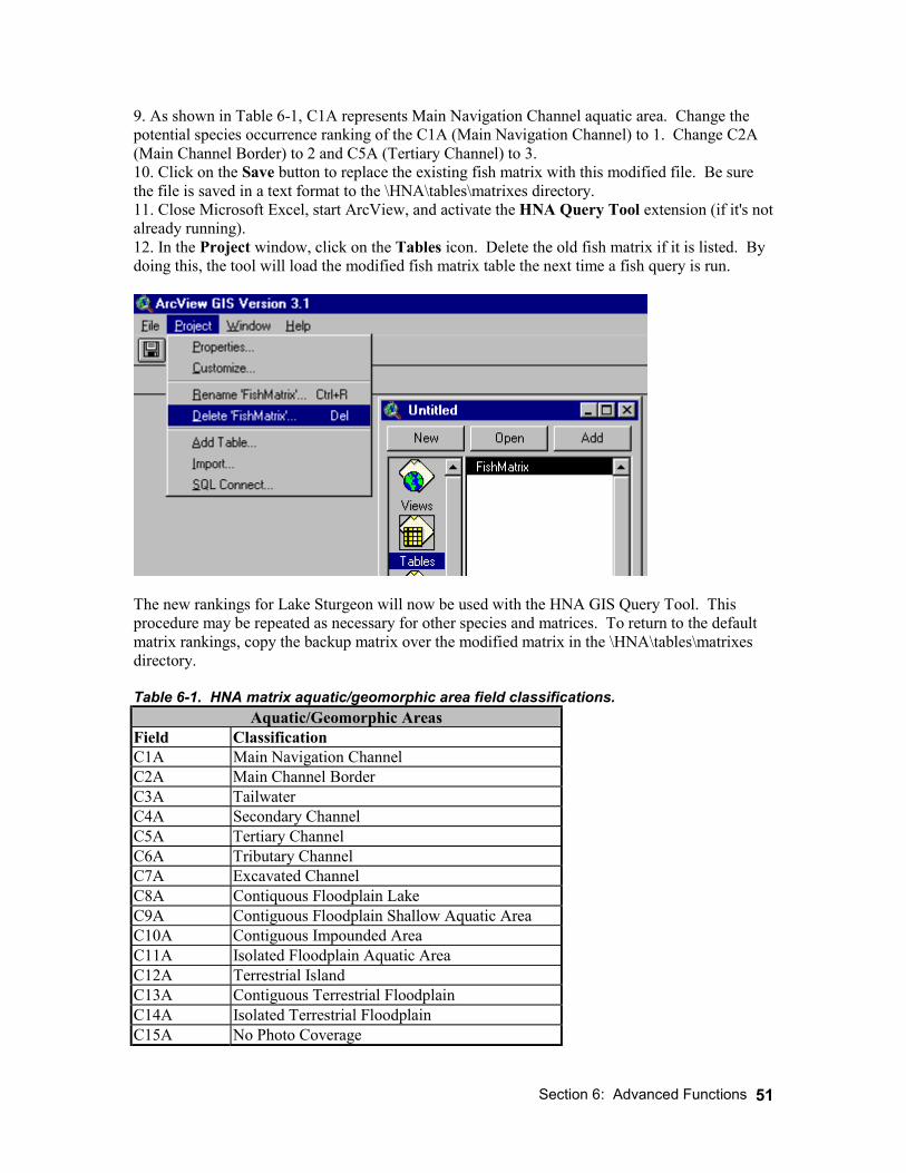
Section 6: Advanced Functions
51
9. As shown in Table 6-1, C1A represents Main Navigation Channel aquatic area. Change the potential species occurrence ranking of the C1A (Main Navigation Channel) to 1. Change C2A (Main Channel Border) to 2 and C5A (Tertiary Channel) to 3. 10. Click on the Save button to replace the existing fish matrix with this modified file. Be sure the file is saved in a text format to the \HNA\tables\matrixes directory. 11. Close Microsoft Excel, start ArcView, and activate the HNA Query Tool extension (if it's not already running). 12. In the Project window, click on the Tables icon. Delete the old fish matrix if it is listed. By doing this, the tool will load the modified fish matrix table the next time a fish query is run.
The new rankings for Lake Sturgeon will now be used with the HNA GIS Query Tool. This procedure may be repeated as necessary for other species and matrices. To return to the default matrix rankings, copy the backup matrix over the modified matrix in the \HNA\tables\matrixes directory. Table 6-1. HNA matrix aquatic/geomorphic area field classifications.
Aquatic/Geomorphic Areas Field Classification C1A Main Navigation Channel C2A Main Channel Border C3A Tailwater C4A Secondary Channel C5A Tertiary Channel C6A Tributary Channel C7A Excavated Channel C8A Contiquous Floodplain Lake C9A Contiguous Floodplain Shallow Aquatic Area C10A Contiguous Impounded Area C11A Isolated Floodplain Aquatic Area C12A Terrestrial Island C13A Contiguous Terrestrial Floodplain C14A Isolated Terrestrial Floodplain C15A No Photo Coverage

Section 6: Advanced Functions
52
Moving Products to Other Applications (e.g., MS Word, PowerPoint, or Excel) The graphic and tabular products generated by the HNA GIS Query Tool can be moved to other computer applications. Graphic information may be moved from an ArcView Layout document to other applications (e.g., MS Word and/or PowerPoint) by using the following process. 1. Start ArcView and Microsoft PowerPoint. 2. In ArcView, open an existing Layout document, or create a new one with added map elements. 3. With the Layout document active, click on the Pointer button. 4. Select the graphic element you wish to move by clicking on it. Multiple elements may be selected by holding down the Shift key while clicking on them.
5. In the Edit menu select Copy. Please wait a few seconds when copying large complex map elements. 6. Minimize ArcView. 7. In PowerPoint, insert a new blank slide (if needed). 8. Click on Paste in the Edit menu. The map elements are now displayed on the PowerPoint slide. They may be moved and resized as necessary.
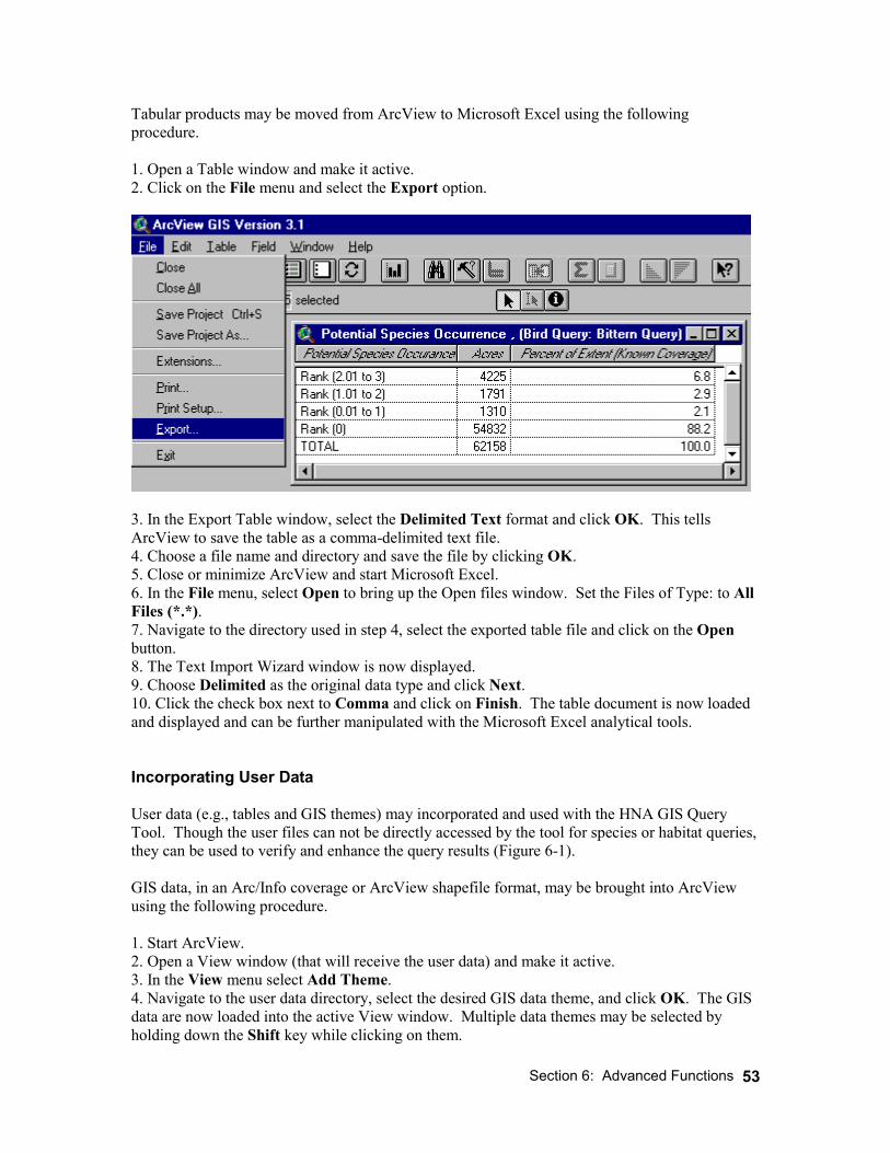
Section 6: Advanced Functions
53
Tabular products may be moved from ArcView to Microsoft Excel using the following procedure. 1. Open a Table window and make it active. 2. Click on the File menu and select the Export option.
3. In the Export Table window, select the Delimited Text format and click OK. This tells ArcView to save the table as a comma-delimited text file. 4. Choose a file name and directory and save the file by clicking OK. 5. Close or minimize ArcView and start Microsoft Excel. 6. In the File menu, select Open to bring up the Open files window. Set the Files of Type: to All Files (*.*). 7. Navigate to the directory used in step 4, select the exported table file and click on the Open button. 8. The Text Import Wizard window is now displayed. 9. Choose Delimited as the original data type and click Next. 10. Click the check box next to Comma and click on Finish. The table document is now loaded and displayed and can be further manipulated with the Microsoft Excel analytical tools. Incorporating User Data User data (e.g., tables and GIS themes) may incorporated and used with the HNA GIS Query Tool. Though the user files can not be directly accessed by the tool for species or habitat queries, they can be used to verify and enhance the query results (Figure 6-1). GIS data, in an Arc/Info coverage or ArcView shapefile format, may be brought into ArcView using the following procedure. 1. Start ArcView. 2. Open a View window (that will receive the user data) and make it active. 3. In the View menu select Add Theme. 4. Navigate to the user data directory, select the desired GIS data theme, and click OK. The GIS data are now loaded into the active View window. Multiple data themes may be selected by holding down the Shift key while clicking on them.
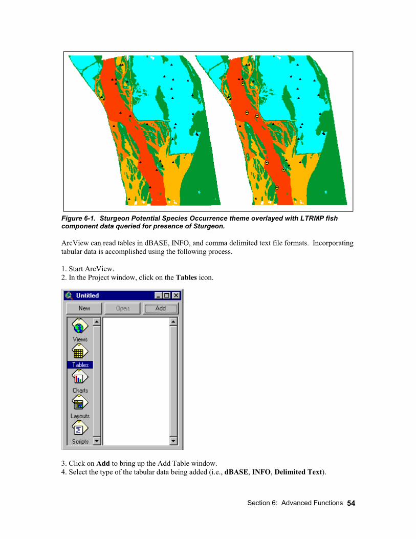
Section 6: Advanced Functions
54
Figure 6-1. Sturgeon Potential Species Occurrence theme overlayed with LTRMP fish component data queried for presence of Sturgeon. ArcView can read tables in dBASE, INFO, and comma delimited text file formats. Incorporating tabular data is accomplished using the following process. 1. Start ArcView. 2. In the Project window, click on the Tables icon.
3. Click on Add to bring up the Add Table window. 4. Select the type of the tabular data being added (i.e., dBASE, INFO, Delimited Text).
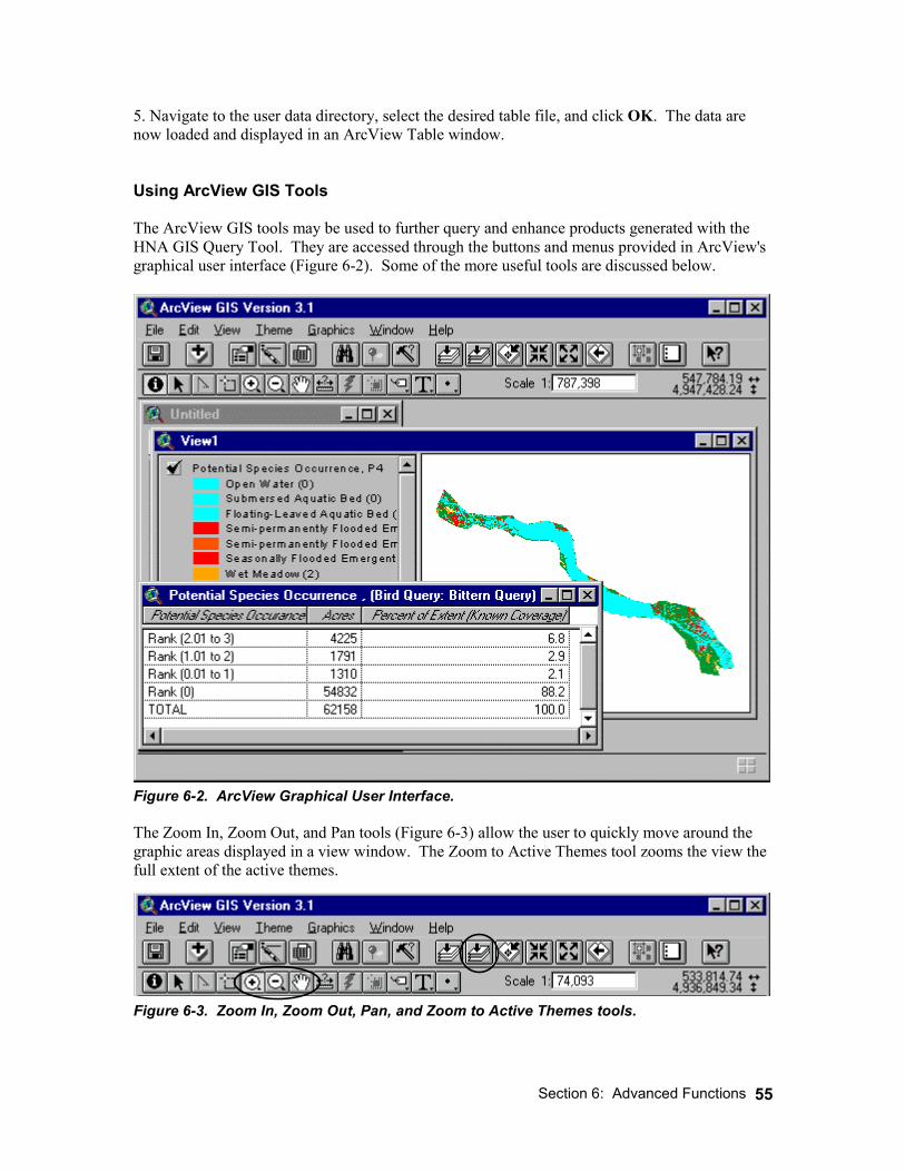
Section 6: Advanced Functions
55
5. Navigate to the user data directory, select the desired table file, and click OK. The data are now loaded and displayed in an ArcView Table window. Using ArcView GIS Tools The ArcView GIS tools may be used to further query and enhance products generated with the HNA GIS Query Tool. They are accessed through the buttons and menus provided in ArcView's graphical user interface (Figure 6-2). Some of the more useful tools are discussed below.
Figure 6-2. ArcView Graphical User Interface. The Zoom In, Zoom Out, and Pan tools (Figure 6-3) allow the user to quickly move around the graphic areas displayed in a view window. The Zoom to Active Themes tool zooms the view the full extent of the active themes.
Figure 6-3. Zoom In, Zoom Out, Pan, and Zoom to Active Themes tools.
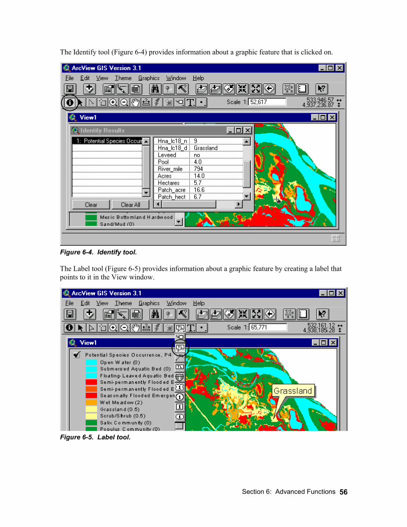
Section 6: Advanced Functions
56
The Identify tool (Figure 6-4) provides information about a graphic feature that is clicked on.
Figure 6-4. Identify tool. The Label tool (Figure 6-5) provides information about a graphic feature by creating a label that points to it in the View window.
Figure 6-5. Label tool.
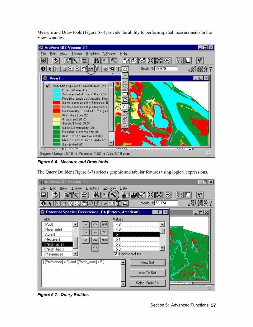
Section 6: Advanced Functions
57
Measure and Draw tools (Figure 6-6) provide the ability to perform spatial measurements in the View window.
Figure 6-6. Measure and Draw tools. The Query Builder (Figure 6-7) selects graphic and tabular features using logical expressions.
Figure 6-7. Query Builder.
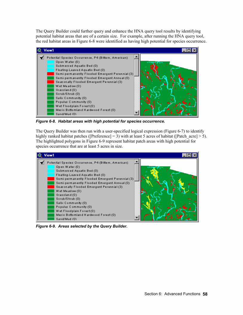
Section 6: Advanced Functions
58
The Query Builder could further query and enhance the HNA query tool results by identifying potential habitat areas that are of a certain size. For example, after running the HNA query tool, the red habitat areas in Figure 6-8 were identified as having high potential for species occurrence.
Figure 6-8. Habitat areas with high potential for species occurrence. The Query Builder was then run with a user-specified logical expression (Figure 6-7) to identify highly ranked habitat patches ([Preference] = 3) with at least 5 acres of habitat ([Patch_acre] > 5). The highlighted polygons in Figure 6-9 represent habitat patch areas with high potential for species occurrence that are at least 5 acres in size.
Figure 6-9. Areas selected by the Query Builder.
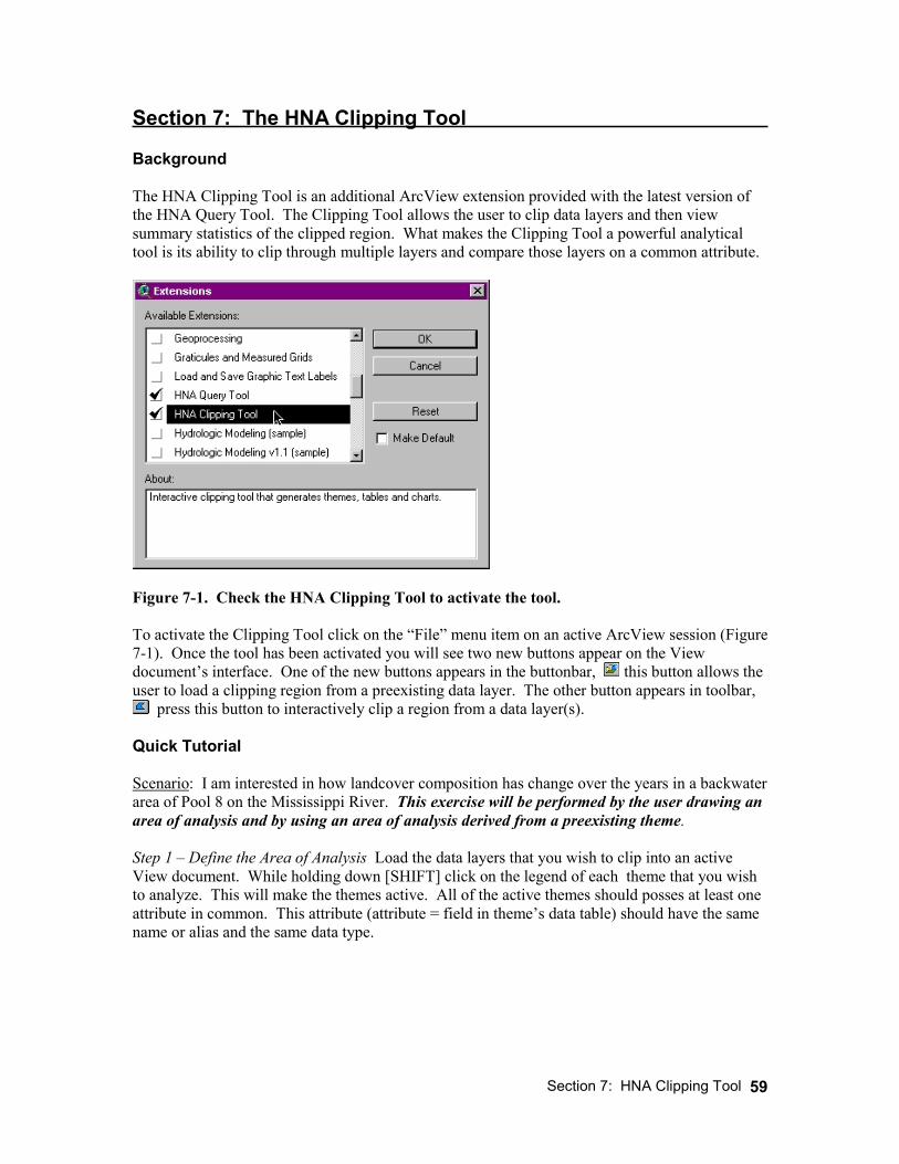
Section 7: HNA Clipping Tool
59
Section 7: The HNA Clipping Tool Background The HNA Clipping Tool is an additional ArcView extension provided with the latest version of the HNA Query Tool. The Clipping Tool allows the user to clip data layers and then view summary statistics of the clipped region. What makes the Clipping Tool a powerful analytical tool is its ability to clip through multiple layers and compare those layers on a common attribute.
Figure 7-1. Check the HNA Clipping Tool to activate the tool. To activate the Clipping Tool click on the “File” menu item on an active ArcView session (Figure 7-1). Once the tool has been activated you will see two new buttons appear on the View document’s interface. One of the new buttons appears in the buttonbar, this button allows the user to load a clipping region from a preexisting data layer. The other button appears in toolbar,
press this button to interactively clip a region from a data layer(s). Quick Tutorial Scenario: I am interested in how landcover composition has change over the years in a backwater area of Pool 8 on the Mississippi River. This exercise will be performed by the user drawing an area of analysis and by using an area of analysis derived from a preexisting theme. Step 1 – Define the Area of Analysis Load the data layers that you wish to clip into an active View document. While holding down [SHIFT] click on the legend of each theme that you wish to analyze. This will make the themes active. All of the active themes should posses at least one attribute in common. This attribute (attribute = field in theme’s data table) should have the same name or alias and the same data type.
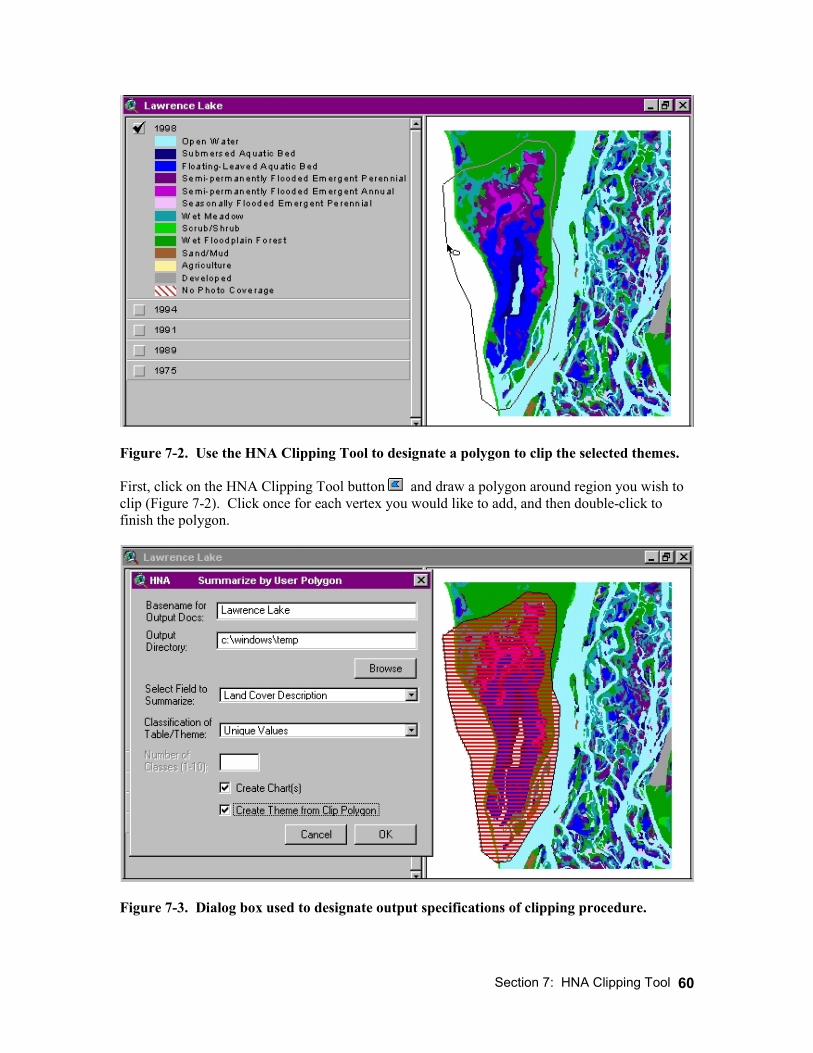
Section 7: HNA Clipping Tool
60
Figure 7-2. Use the HNA Clipping Tool to designate a polygon to clip the selected themes. First, click on the HNA Clipping Tool button and draw a polygon around region you wish to clip (Figure 7-2). Click once for each vertex you would like to add, and then double-click to finish the polygon.
Figure 7-3. Dialog box used to designate output specifications of clipping procedure.
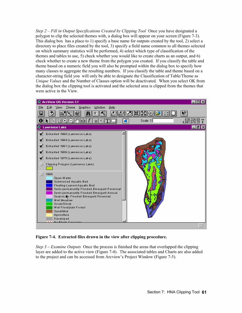
Section 7: HNA Clipping Tool
61
Step 2 – Fill in Output Specifications Created by Clipping Tool Once you have designated a polygon to clip the selected themes with, a dialog box will appear on your screen (Figure 7-3). This dialog box has a place to 1) specify a base name for outputs created by the tool, 2) select a directory to place files created by the tool, 3) specify a field name common to all themes selected on which summary statistics will be performed, 4) select which type of classification of the themes and tables to use, 5) check whether you would like to create charts as an output, and 6) check whether to create a new theme from the polygon you created. If you classify the table and theme based on a numeric field you will also be prompted within the dialog box to specify how many classes to aggregate the resulting numbers. If you classify the table and theme based on a character-string field you will only be able to designate the Classification of Table/Theme as Unique Values and the Number of Classes option will be deactivated. When you select OK from the dialog box the clipping tool is activated and the selected area is clipped from the themes that were active in the View.
Figure 7-4. Extracted files drawn in the view after clipping procedure. Step 3 – Examine Outputs Once the process is finished the areas that overlapped the clipping layer are added to the active view (Figure 7-4). The associated tables and Charts are also added to the project and can be accessed from Arcview’s Project Window (Figure 7-5).
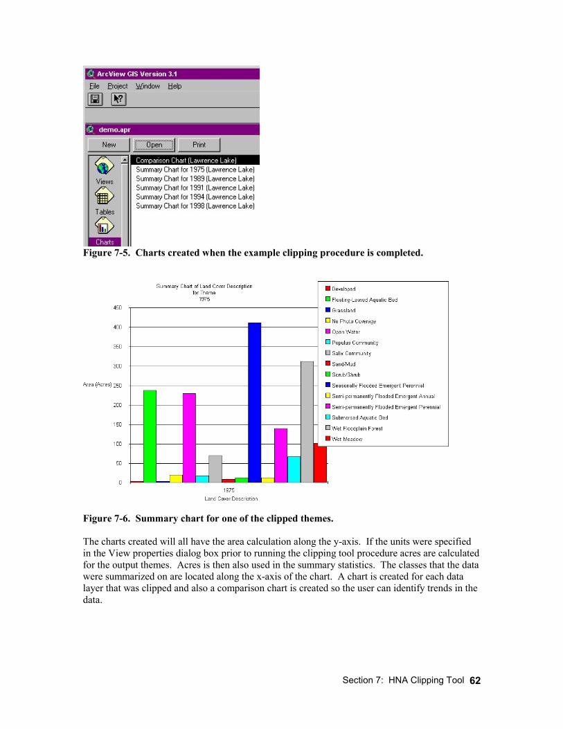
Section 7: HNA Clipping Tool
62
Figure 7-5. Charts created when the example clipping procedure is completed.
Figure 7-6. Summary chart for one of the clipped themes. The charts created will all have the area calculation along the y-axis. If the units were specified in the View properties dialog box prior to running the clipping tool procedure acres are calculated for the output themes. Acres is then also used in the summary statistics. The classes that the data were summarized on are located along the x-axis of the chart. A chart is created for each data layer that was clipped and also a comparison chart is created so the user can identify trends in the data.
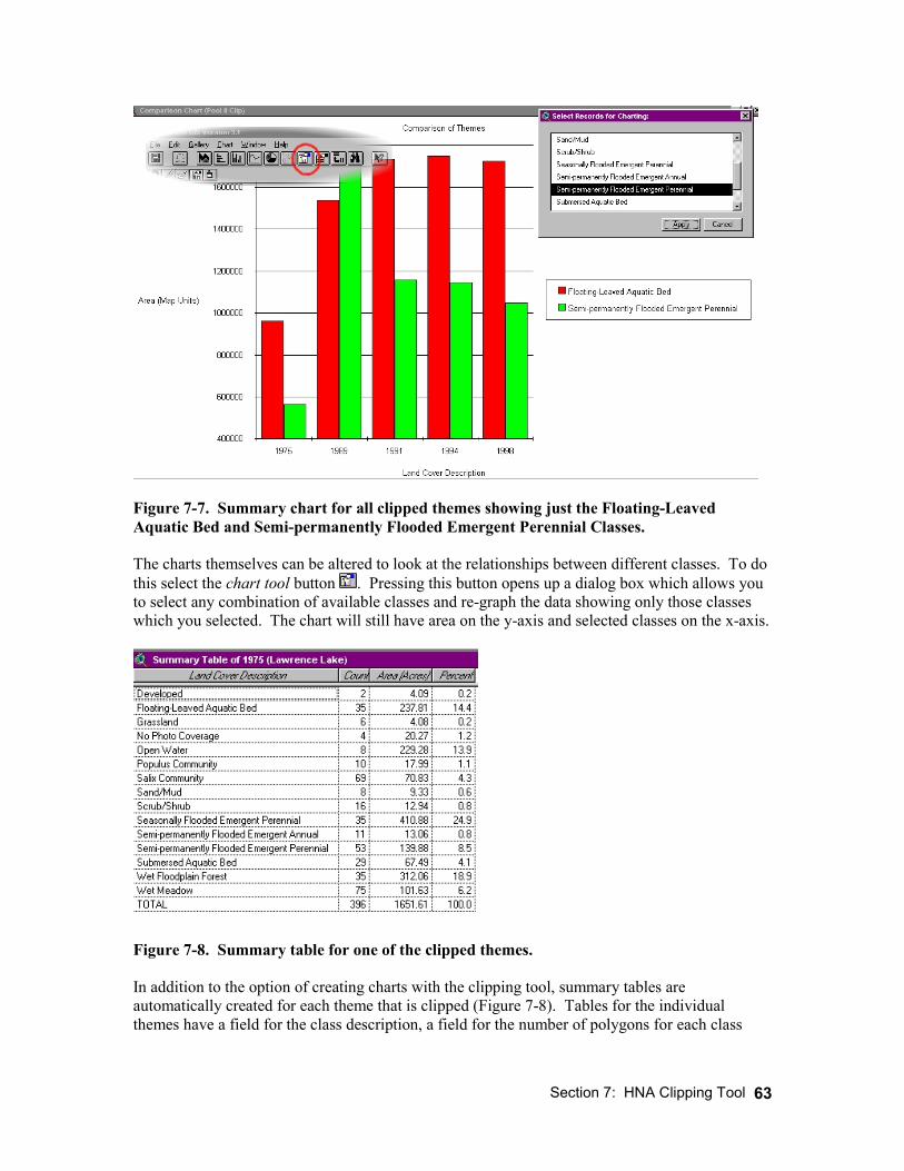
Section 7: HNA Clipping Tool
63
Figure 7-7. Summary chart for all clipped themes showing just the Floating-Leaved Aquatic Bed and Semi-permanently Flooded Emergent Perennial Classes. The charts themselves can be altered to look at the relationships between different classes. To do this select the chart tool button . Pressing this button opens up a dialog box which allows you to select any combination of available classes and re-graph the data showing only those classes which you selected. The chart will still have area on the y-axis and selected classes on the x-axis.
Figure 7-8. Summary table for one of the clipped themes. In addition to the option of creating charts with the clipping tool, summary tables are automatically created for each theme that is clipped (Figure 7-8). Tables for the individual themes have a field for the class description, a field for the number of polygons for each class
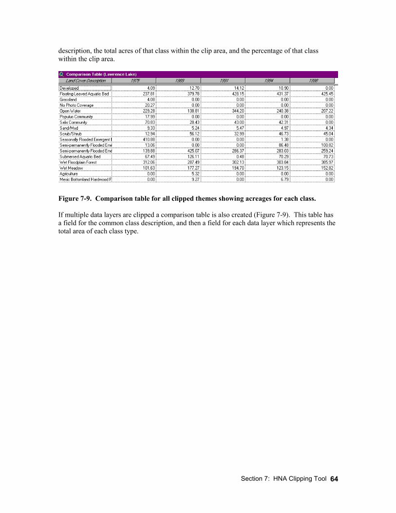
Section 7: HNA Clipping Tool
64
description, the total acres of that class within the clip area, and the percentage of that class within the clip area.
Figure 7-9. Comparison table for all clipped themes showing acreages for each class. If multiple data layers are clipped a comparison table is also created (Figure 7-9). This table has a field for the common class description, and then a field for each data layer which represents the total area of each class type.
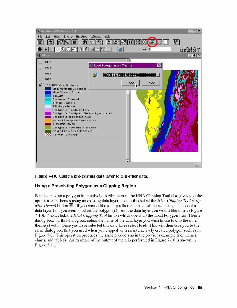
Section 7: HNA Clipping Tool
65
Figure 7-10. Using a pre-existing data layer to clip other data. Using a Preexisting Polygon as a Clipping Region Besides making a polygon interactively to clip themes, the HNA Clipping Tool also gives you the option to clip themes using an existing data layer. To do this select the HNA Clipping Tool (Clip with Theme) button . If you would like to clip a theme or a set of themes using a subset of a data layer first you need to select the polygon(s) from the data layer you would like to use (Figure 7-10). Next, click the HNA Clipping Tool button which opens up the Load Polygon from Theme dialog box. In this dialog box select the name of the data layer you wish to use to clip the other theme(s) with. Once you have selected this data layer select load. This will then take you to the same dialog box that you used when you clipped with an interactively created polygon such as in Figure 7-3. This operation produces the same products as in the previous example (i.e. themes, charts, and tables). An example of the output of the clip performed in Figure 7-10 is shown in Figure 7-11.
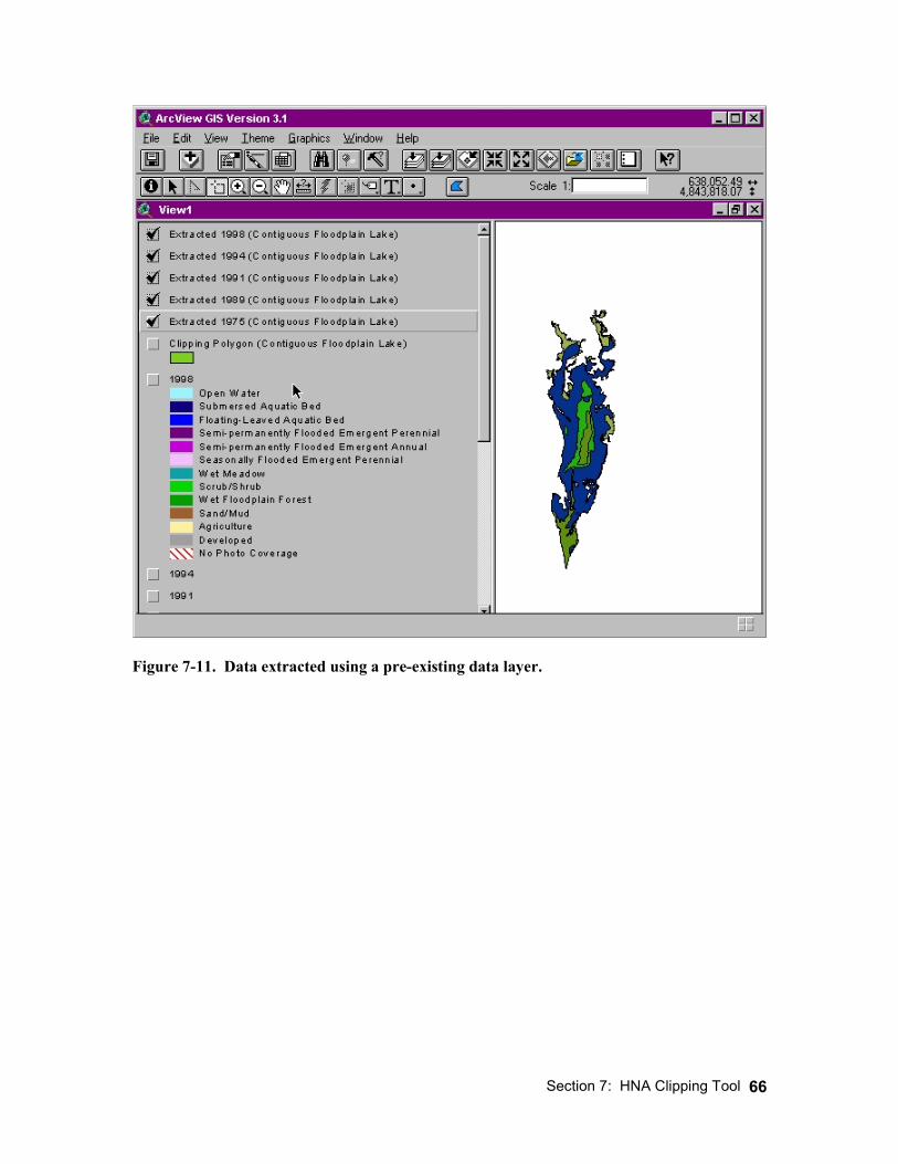
Section 7: HNA Clipping Tool
66
Figure 7-11. Data extracted using a pre-existing data layer.
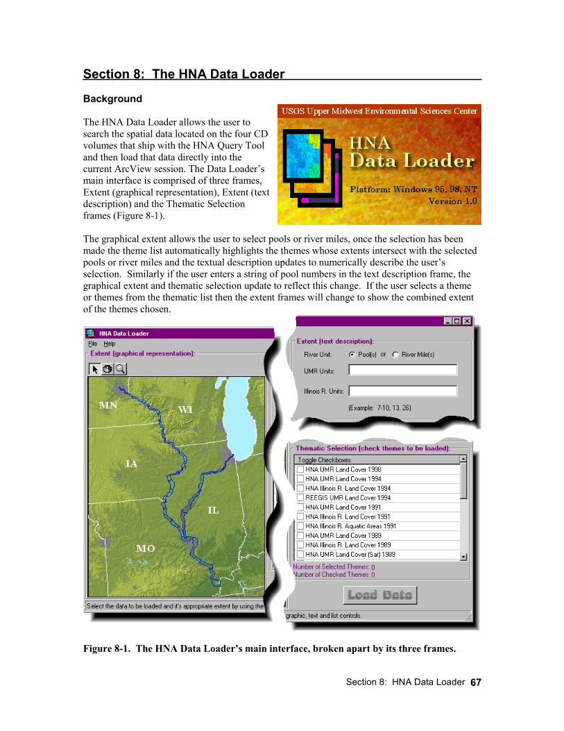
Section 8: HNA Data Loader
67
Section 8: The HNA Data Loader Background The HNA Data Loader allows the user to search the spatial data located on the four CD volumes that ship with the HNA Query Tool and then load that data directly into the current ArcView session. The Data Loader’s main interface is comprised of three frames, Extent (graphical representation), Extent (text description) and the Thematic Selection frames (Figure 8-1). The graphical extent allows the user to select pools or river miles, once the selection has been made the theme list automatically highlights the themes whose extents intersect with the selected pools or river miles and the textual description updates to numerically describe the user’s selection. Similarly if the user enters a string of pool numbers in the text description frame, the graphical extent and thematic selection update to reflect this change. If the user selects a theme or themes from the thematic list then the extent frames will change to show the combined extent of the themes chosen.
Figure 8-1. The HNA Data Loader’s main interface, broken apart by its three frames.
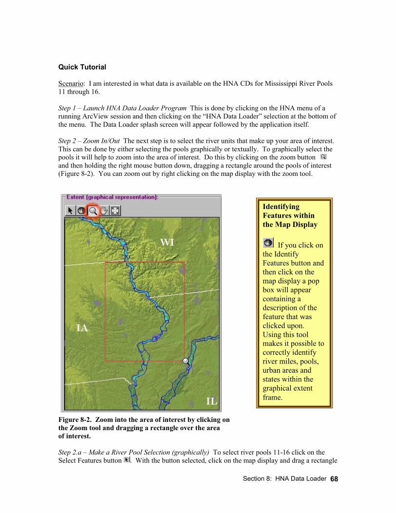
Section 8: HNA Data Loader
68
Quick Tutorial Scenario: I am interested in what data is available on the HNA CDs for Mississippi River Pools 11 through 16. Step 1 – Launch HNA Data Loader Program This is done by clicking on the HNA menu of a running ArcView session and then clicking on the “HNA Data Loader” selection at the bottom of the menu. The Data Loader splash screen will appear followed by the application itself. Step 2 – Zoom In/Out The next step is to select the river units that make up your area of interest. This can be done by either selecting the pools graphically or textually. To graphically select the pools it will help to zoom into the area of interest. Do this by clicking on the zoom button and then holding the right mouse button down, dragging a rectangle around the pools of interest (Figure 8-2). You can zoom out by right clicking on the map display with the zoom tool.
Figure 8-2. Zoom into the area of interest by clicking on the Zoom tool and dragging a rectangle over the area of interest. Step 2.a – Make a River Pool Selection (graphically) To select river pools 11-16 click on the Select Features button . With the button selected, click on the map display and drag a rectangle
Identifying Features within the Map Display
If you click on the Identify Features button and then click on the map display a pop box will appear containing a description of the feature that was clicked upon. Using this tool makes it possible to correctly identify river miles, pools, urban areas and states within the graphical extent frame.
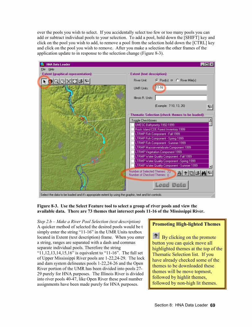
Section 8: HNA Data Loader
69
over the pools you wish to select. If you accidentally select too few or too many pools you can add or subtract individual pools to your selection. To add a pool, hold down the [SHIFT] key and click on the pool you wish to add, to remove a pool from the selection hold down the [CTRL] key and click on the pool you wish to remove. After you make a selection the other frames of the application update to in response to the selection change (Figure 8-3).
Figure 8-3. Use the Select Feature tool to select a group of river pools and view the available data. There are 73 themes that intersect pools 11-16 of the Mississippi River. Step 2.b – Make a River Pool Selection (text description) A quicker method of selected the desired pools would be t simply enter the string “11-16” in the UMR Units textbox located in Extent (text description) frame. When you enter a string, ranges are separated with a dash and commas separate individual pools. Therefore the string “11,12,13,14,15,16” is equivalent to “11-16”. The full set of Upper Mississippi River pools are 1-22,24-29. The lock and dam system delineates pools 1-22,24-26 and the Open River portion of the UMR has been divided into pools 27-29 purely for HNA purposes. The Illinois River is divided into river pools 40-47, like Open River these pool number assignments have been made purely for HNA purposes.
Promoting High-lighted Themes
By clicking on the promote button you can quick move all highlighted themes at the top of the Thematic Selection list. If you have already checked some of the themes to be downloaded these themes will be move topmost, followed by highlit themes, followed by non-high lit themes.
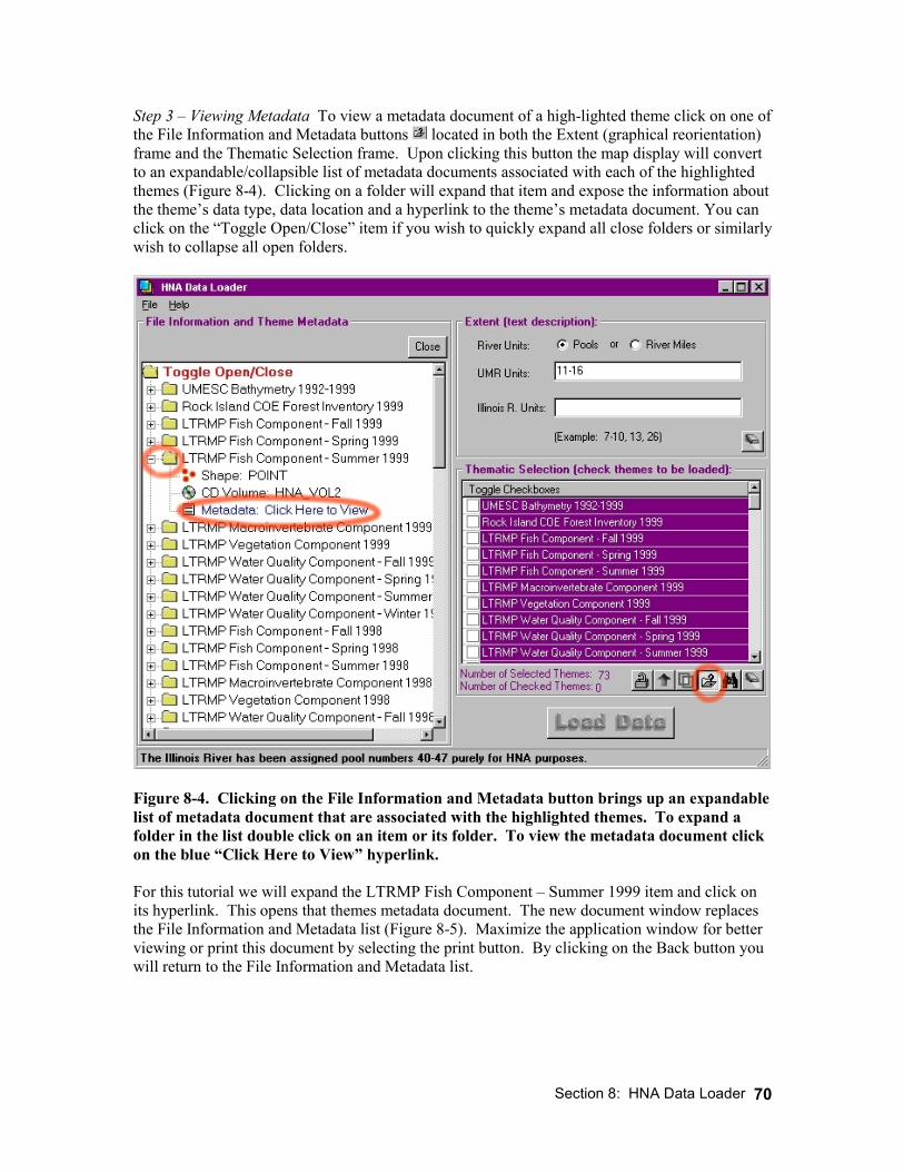
Section 8: HNA Data Loader
70
Step 3 – Viewing Metadata To view a metadata document of a high-lighted theme click on one of the File Information and Metadata buttons located in both the Extent (graphical reorientation) frame and the Thematic Selection frame. Upon clicking this button the map display will convert to an expandable/collapsible list of metadata documents associated with each of the highlighted themes (Figure 8-4). Clicking on a folder will expand that item and expose the information about the theme’s data type, data location and a hyperlink to the theme’s metadata document. You can click on the “Toggle Open/Close” item if you wish to quickly expand all close folders or similarly wish to collapse all open folders.
Figure 8-4. Clicking on the File Information and Metadata button brings up an expandable list of metadata document that are associated with the highlighted themes. To expand a folder in the list double click on an item or its folder. To view the metadata document click on the blue “Click Here to View” hyperlink. For this tutorial we will expand the LTRMP Fish Component – Summer 1999 item and click on its hyperlink. This opens that themes metadata document. The new document window replaces the File Information and Metadata list (Figure 8-5). Maximize the application window for better viewing or print this document by selecting the print button. By clicking on the Back button you will return to the File Information and Metadata list.
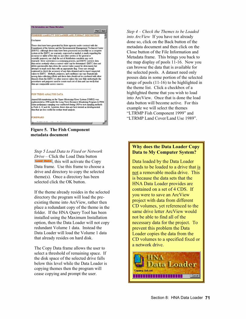
Section 8: HNA Data Loader
71
Step 4 – Check the Themes to be Loaded into ArcView If you have not already done so, click on the Back button of the metadata document and then click on the Close button of the File Information and Metadata frame. This brings you back to the map display of pools 11-16. Now you can browse the data that is available for the selected pools. A dataset need only posses data in some portion of the selected range of pools (11-16) to be highlighted in the theme list. Click a checkbox of a highlighted theme that you wish to load into ArcView. Once that is done the load data button will become active. For this example we will select the themes “LTRMP Fish Component 1999” and “LTRMP Land Cover/Land Use 1989”.
Step 5 Load Data to Fixed or Network Drive – Click the Load Data button
, this will activate the Copy Data frame. Use this frame to choose a drive and directory to copy the selected theme(s). Once a directory has been selected click the OK button. If the theme already resides in the selected directory the program will load the pre-existing theme into ArcView, rather then place a redundant copy of the theme in the folder. If the HNA Query Tool has been installed using the Maximum Installation option, then the Data Loader will not copy redundant Volume 1 data. Instead the Data Loader will load the Volume 1 data that already resides on hard disk. The Copy Data frame allows the user to select a threshold of remaining space. If the disk space of the selected drive falls below this level while the Data Loader is copying themes then the program will cease copying and prompt the user.
Figure 5. The Fish Component metadata document
Why does the Data Loader Copy Data to My Computer System? Data loaded by the Data Loader needs to be loaded to a drive that is not a removable media drive. This is because the data sets that the HNA Data Loader provides are contained on a set of 4 CDS. If you were to save an ArcView project with data from different CD volumes, yet referenced to the same drive letter ArcView would not be able to find all of the necessary data for the project. To prevent this problem the Data Loader copies the data from the CD volumes to a specified fixed or a network drive.
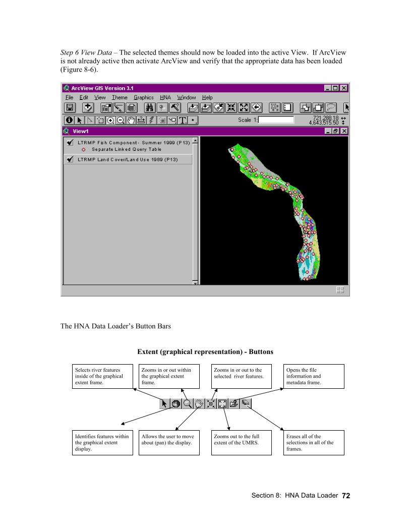
Section 8: HNA Data Loader
72
Step 6 View Data – The selected themes should now be loaded into the active View. If ArcView is not already active then activate ArcView and verify that the appropriate data has been loaded (Figure 8-6).
The HNA Data Loader’s Button Bars
Extent (graphical representation) - Buttons
Selects river features inside of the graphical extent frame.
Zooms in or out within the graphical extent frame.
Zooms in or out to the selected river features.
Opens the file information and metadata frame.
Identifies features within the graphical extent display.
Allows the user to move about (pan) the display.
Zooms out to the full extent of the UMRS.
Erases all of the selections in all of the frames.

Section 8: HNA Data Loader
73
Thematic Selection - Buttons
Locks the thematic selection to the currently selected themes. All other themes are made unavailable.
Finds the river pools or river miles were the selected themes intersect (overlap).
Allows the user to find themes by a title or keyword search.
Promotes all selected themes to the top of the theme list.
Opens the file information and metadata frame.
Erases all of the selections in all of the frames.

A-1
Appendix A: Land Cover Cross-walk Tables Table A-1. HNA/LTRMP land cover cross-walk table. HNA Classification LTRMP Classification Open Water Azolla, Lemnaceae, Open Water Submersed Aquatic Bed Azolla/submergents, Ceratophyllum, Elodea,
Lemnaceae/Ceratophyllum, Lemna/Ceratophyll/Potamogeton, Lemnaceae/submergents, Myrioph/Potamoget/Vallis, Myriophyllum, Myriophyllum/Zosterella, Potamogeton, Potamoget/Vallis/Zost/Cerat, Submergents, Vallisneria, Vallisneria/Potamogeton, Vallisneria/Potamoget/Heteran, Vallisneria/Zosterella, Zosterella
Floating-Leaved Aquatic Bed
Brasenia, Brasenia/submergents, Jussiaea, Nelumbo, Nelumbo/Lemnaceae, Nelumbo/Myriophyllum, Nelumbo/Nymphaea, Nelumbo/Nymphaea/Lemnaceae, Nelumbo/Nymphaea/Myriophyllum, Nelumbo/Nymphaea/submerg/Lemn, Nelumbo/submergents, Nelumbo/submergents/Lemnaceae, Nuphar, Nuphar/Nympheae/submergents, Nuphar/submergents, Nymphaea, Nymphaea/Ceratophyllum/Lemna, Nymph/Ceratoph/Myriophyl/Lemna, Nymphaea/Lemnaceae, Nymphaea/Myriophyllum, Nymphaea/Nelumbo/submergents, Nymphaea/submergents, Nymphaea/submergents/Lemnaceae
Semi-permanently Flooded Emergent Annual
Nympheaea/Zizania, Nymphaea/Zizania/submergents, Zizania, Zizania/Nymphaea/Nelumbo/sub
Semi-permanently Flooded Emergent Perennial
Acorus, Nelum/Nymph/Ponted/sub/Lemn, Nelumbo/Nymphaea/Sagittaria, Nelum/Nymph/Sag/Sparg/sub/Lemn, Nelumbo/Nympheae/Sagittaria/submergents, Nelumbo/Sagittaria/submergents, Nymphaea/Sagittaria, Nymphaea/Scirpus, Phragmites, Polygonum, Polygonum/Nelumbo, Pontederia, Pontederia/Nymph/Nelumbo/sub, Sagittaria, Sagittaria/Ceratophyllum/Lemnaceae, Sagittaria/Lemnaceae, Sagittaria/Nelumbo, Sagittaria/Scirpus/Sparganium, Sagittaria/Sparganium, Scirpus, Scirpus/Lythrum, Scirpus/Nelumbo/submergents, Scirpus/Nymphaea/submergents, Scirpus/Phalaris, Scirpus/Phragmites, Scirpus/Polygonum, Scirpus/Sagittaria, Scirpus/Sparganium, Scirpus/Typha/Phalaris, Scirpus/Zizania, Sparganium, Typha, Typha/Lythrum, Typha/Lythrum/Phragmites, Typha/Sagittaria, Typha/Sagittaria/Scirpus, Typha/Sagittaria/Scirpus/Sparganium, Typha/Sagittaria/Sparganium, Typha/Scirpus, Typha/Scirpus/Sparganium, Typha/Sparganium
Seasonally Flooded Emergent Annual
NA
Seasonally Flooded Emergent Perennial
Cyperus, Echinodorus, Eleocharis, Leersia/Sagittaria, Sagittaria/Phalaris, Sagittaria/Polygonum, Sag/Sparg/Typ/Scirp/Leer/Phrag
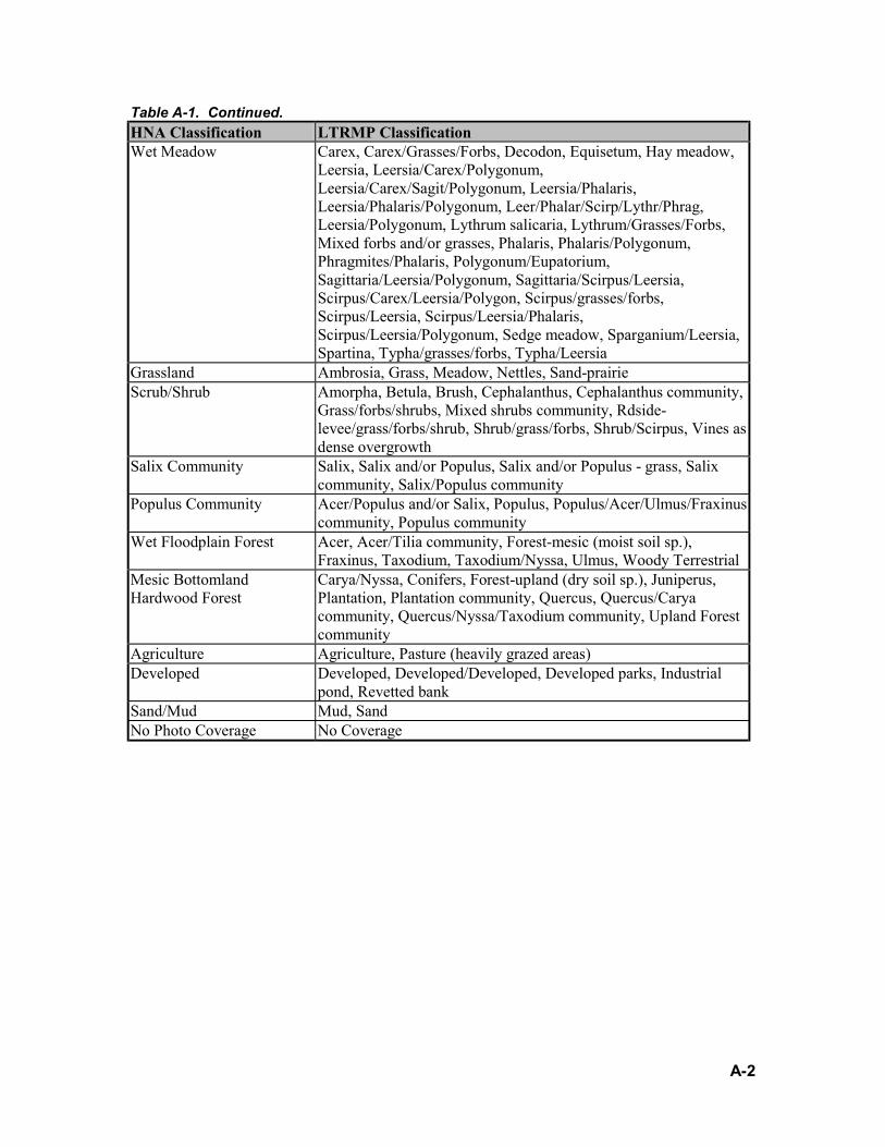
A-2
Table A-1. Continued. HNA Classification LTRMP Classification Wet Meadow Carex, Carex/Grasses/Forbs, Decodon, Equisetum, Hay meadow,
Leersia, Leersia/Carex/Polygonum, Leersia/Carex/Sagit/Polygonum, Leersia/Phalaris, Leersia/Phalaris/Polygonum, Leer/Phalar/Scirp/Lythr/Phrag, Leersia/Polygonum, Lythrum salicaria, Lythrum/Grasses/Forbs, Mixed forbs and/or grasses, Phalaris, Phalaris/Polygonum, Phragmites/Phalaris, Polygonum/Eupatorium, Sagittaria/Leersia/Polygonum, Sagittaria/Scirpus/Leersia, Scirpus/Carex/Leersia/Polygon, Scirpus/grasses/forbs, Scirpus/Leersia, Scirpus/Leersia/Phalaris, Scirpus/Leersia/Polygonum, Sedge meadow, Sparganium/Leersia, Spartina, Typha/grasses/forbs, Typha/Leersia
Grassland Ambrosia, Grass, Meadow, Nettles, Sand-prairie Scrub/Shrub Amorpha, Betula, Brush, Cephalanthus, Cephalanthus community,
Grass/forbs/shrubs, Mixed shrubs community, Rdside-levee/grass/forbs/shrub, Shrub/grass/forbs, Shrub/Scirpus, Vines as dense overgrowth
Salix Community Salix, Salix and/or Populus, Salix and/or Populus - grass, Salix community, Salix/Populus community
Populus Community Acer/Populus and/or Salix, Populus, Populus/Acer/Ulmus/Fraxinus community, Populus community
Wet Floodplain Forest Acer, Acer/Tilia community, Forest-mesic (moist soil sp.), Fraxinus, Taxodium, Taxodium/Nyssa, Ulmus, Woody Terrestrial
Mesic Bottomland Hardwood Forest
Carya/Nyssa, Conifers, Forest-upland (dry soil sp.), Juniperus, Plantation, Plantation community, Quercus, Quercus/Carya community, Quercus/Nyssa/Taxodium community, Upland Forest community
Agriculture Agriculture, Pasture (heavily grazed areas) Developed Developed, Developed/Developed, Developed parks, Industrial
pond, Revetted bank Sand/Mud Mud, Sand No Photo Coverage No Coverage
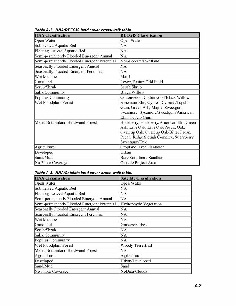
A-3
Table A-2. HNA/REEGIS land cover cross-walk table. HNA Classification REEGIS Classification Open Water Open Water Submersed Aquatic Bed NA Floating-Leaved Aquatic Bed NA Semi-permanently Flooded Emergent Annual NA Semi-permanently Flooded Emergent Perennial Non-Forested Wetland Seasonally Flooded Emergent Annual NA Seasonally Flooded Emergent Perennial NA Wet Meadow Marsh Grassland Levee, Pasture/Old Field Scrub/Shrub Scrub/Shrub Salix Community Black Willow Populus Community Cottonwood, Cottonwood/Black Willow Wet Floodplain Forest American Elm, Cypres, Cypress/Tupelo
Gum, Green Ash, Maple, Sweetgum, Sycamore, Sycamore/Sweetgum/American Elm, Tupelo Gum
Mesic Bottomland Hardwood Forest Hackberry, Hackberry/American Elm/Green Ash, Live Oak, Live Oak/Pecan, Oak, Overcup Oak, Overcup Oak/Bitter Pecan, Pecan, Ridge Slough Complex, Sugarberry, Sweetgum/Oak
Agriculture Cropland, Tree Plantation Developed Urban Sand/Mud Bare Soil, Inert, Sandbar No Photo Coverage Outside Project Area Table A-3. HNA/Satellite land cover cross-walk table. HNA Classification Satellite Classification Open Water Open Water Submersed Aquatic Bed NA Floating-Leaved Aquatic Bed NA Semi-permanently Flooded Emergent Annual NA Semi-permanently Flooded Emergent Perennial Hydrophytic Vegetation Seasonally Flooded Emergent Annual NA Seasonally Flooded Emergent Perennial NA Wet Meadow NA Grassland Grasses/Forbes Scrub/Shrub NA Salix Community NA Populus Community NA Wet Floodplain Forest Woody Terrestrial Mesic Bottomland Hardwood Forest NA Agriculture Agriculture Developed Urban/Developed Sand/Mud Sand No Photo Coverage NoData/Clouds

A-4
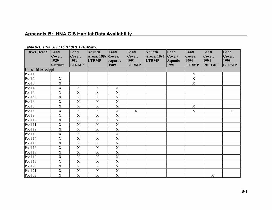
B-1
Appendix B: HNA GIS Habitat Data Availability Table B-1. HNA GIS habitat data availability.
River Reach Land Cover, 1989 Satellite
Land Cover, 1989 LTRMP
Aquatic Areas, 1989 LTRMP
Land Cover/ Aquatic 1989
Land Cover, 1991 LTRMP
Aquatic Areas, 1991 LTRMP
Land Cover/ Aquatic 1991
Land Cover, 1994 LTRMP
Land Cover, 1994 REEGIS
Land Cover, 1998 LTRMP
Upper Mississippi Pool 1 X Pool 2 X X Pool 3 X X Pool 4 X X X X Pool 5 X X X X Pool 5a X X X X Pool 6 X X X X Pool 7 X X X X X Pool 8 X X X X X X X Pool 9 X X X X Pool 10 X X X X Pool 11 X X X X Pool 12 X X X X Pool 13 X X X X Pool 14 X X X X Pool 15 X X X X Pool 16 X X X X Pool 17 X X X X Pool 18 X X X X Pool 19 X X X X Pool 20 X X X X Pool 21 X X X X Pool 22 X X X X X
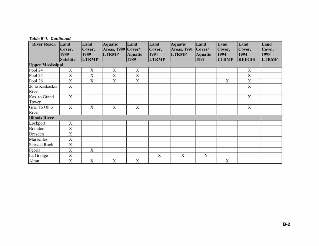
B-2
Table B-1. Continued. River Reach Land
Cover, 1989 Satellite
Land Cover, 1989 LTRMP
Aquatic Areas, 1989 LTRMP
Land Cover/ Aquatic 1989
Land Cover, 1991 LTRMP
Aquatic Areas, 1991 LTRMP
Land Cover/ Aquatic 1991
Land Cover, 1994 LTRMP
Land Cover, 1994 REEGIS
Land Cover, 1998 LTRMP
Upper Mississippi Pool 24 X X X X X Pool 25 X X X X X Pool 26 X X X X X X 26 to Kaskaskia River
X X
Kas. to Grand Tower
X X
Gra. To Ohio River
X X X X X
Illinois River Lockport X Brandon X Dresden X Marseilles X Starved Rock X Peoria X X La Grange X X X X Alton X X X X X

C-1
Appendix C: HNA GIS Query Tool Product Descriptions
Figure C-1. Query report.
The Query Report contains information about the query parameters and results. It includes the following sections. Date: Date the query was run. Results Directory: Location of files generated by the query. Files Written to Results Directory: Description of files generated by the query. Selected Geographic Data Parameters: Information about the GIS habitat data used and the spatial extent of the query. Selected Query Parameters: Description of the parameters used in setting up the query. Individual Species Habitat Preference: Habitat rankings for each queried species. Habitat Class Information: Breakdown of habitat information for the queried extent of the river. Individual Pool Characteristics: Habitat and species characteristics of each queried pool or river mile.
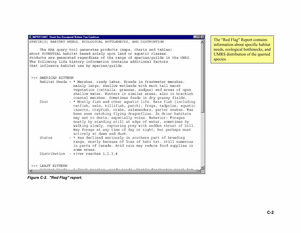
C-2
Figure C-2. "Red Flag" report.
The "Red Flag" Report contains information about specific habitat needs, ecological bottlenecks, and UMRS distribution of the queried species.
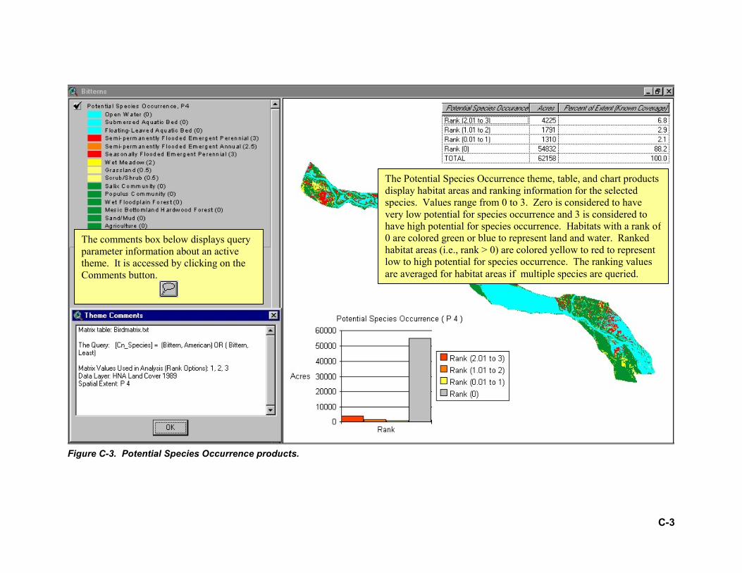
C-3
Figure C-3. Potential Species Occurrence products.
The Potential Species Occurrence theme, table, and chart products display habitat areas and ranking information for the selected species. Values range from 0 to 3. Zero is considered to have very low potential for species occurrence and 3 is considered to have high potential for species occurrence. Habitats with a rank of0 are colored green or blue to represent land and water. Ranked habitat areas (i.e., rank > 0) are colored yellow to red to represent low to high potential for species occurrence. The ranking values are averaged for habitat areas if multiple species are queried.
The comments box below displays query parameter information about an active theme. It is accessed by clicking on the Comments button.
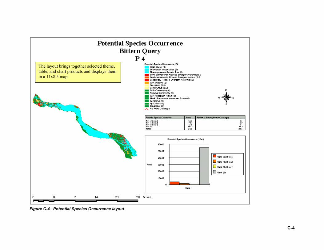
C-4
Figure C-4. Potential Species Occurrence layout.
The layout brings together selected theme, table, and chart products and displays them in a 11x8.5 map.
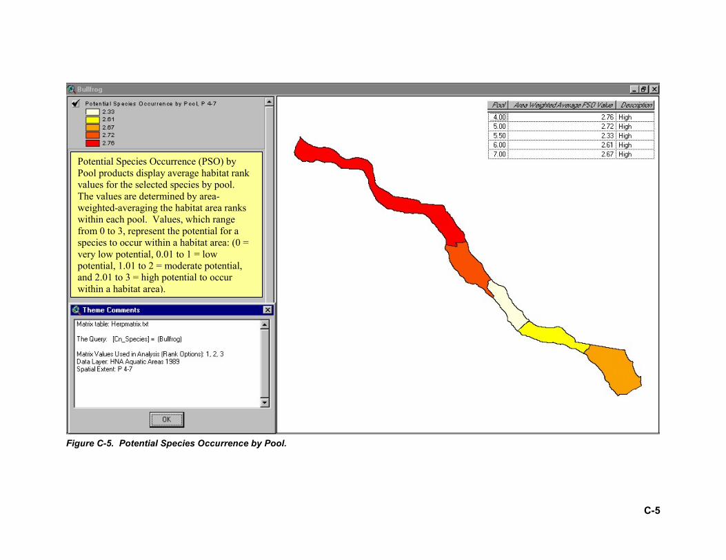
C-5
Figure C-5. Potential Species Occurrence by Pool.
Potential Species Occurrence (PSO) by Pool products display average habitat rank values for the selected species by pool. The values are determined by area-weighted-averaging the habitat area ranks within each pool. Values, which range from 0 to 3, represent the potential for a species to occur within a habitat area: (0 = very low potential, 0.01 to 1 = low potential, 1.01 to 2 = moderate potential, and 2.01 to 3 = high potential to occur within a habitat area).
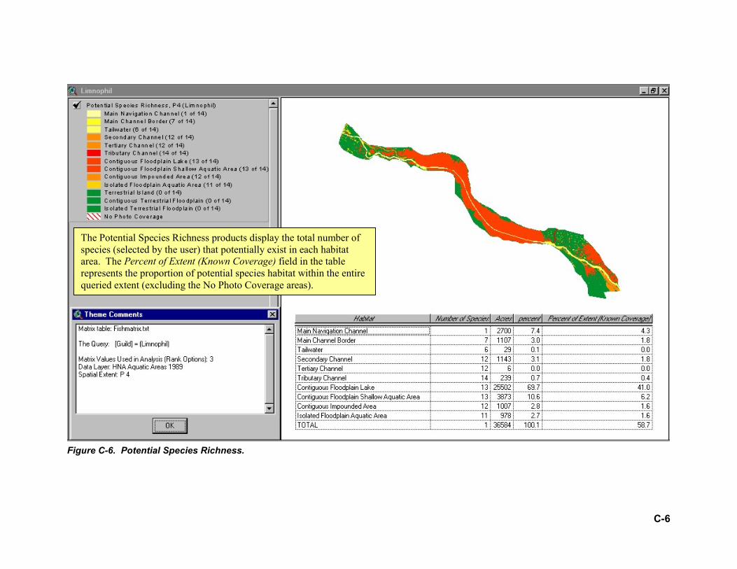
C-6
Figure C-6. Potential Species Richness.
The Potential Species Richness products display the total number of species (selected by the user) that potentially exist in each habitat area. The Percent of Extent (Known Coverage) field in the table represents the proportion of potential species habitat within the entire queried extent (excluding the No Photo Coverage areas).
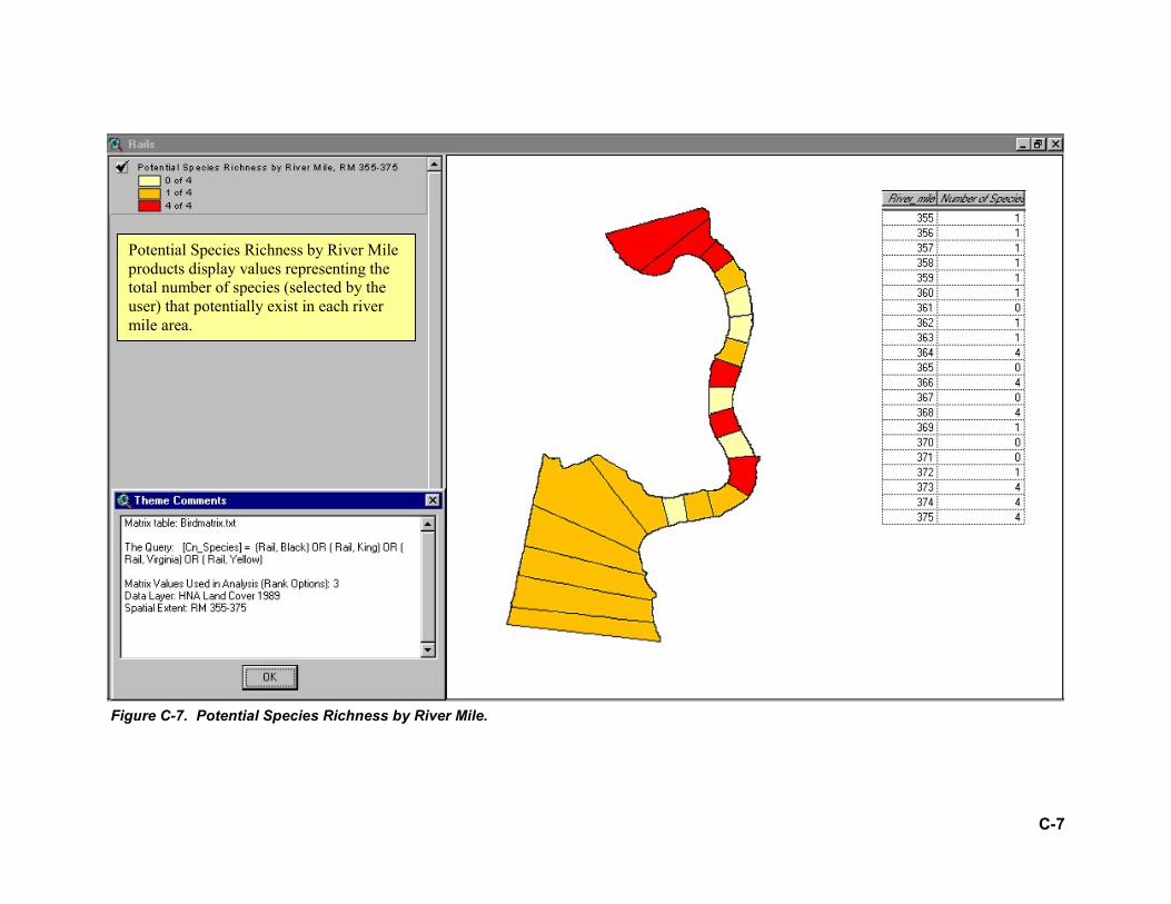
C-7
Figure C-7. Potential Species Richness by River Mile.
Potential Species Richness by River Mile products display values representing the total number of species (selected by the user) that potentially exist in each river mile area.
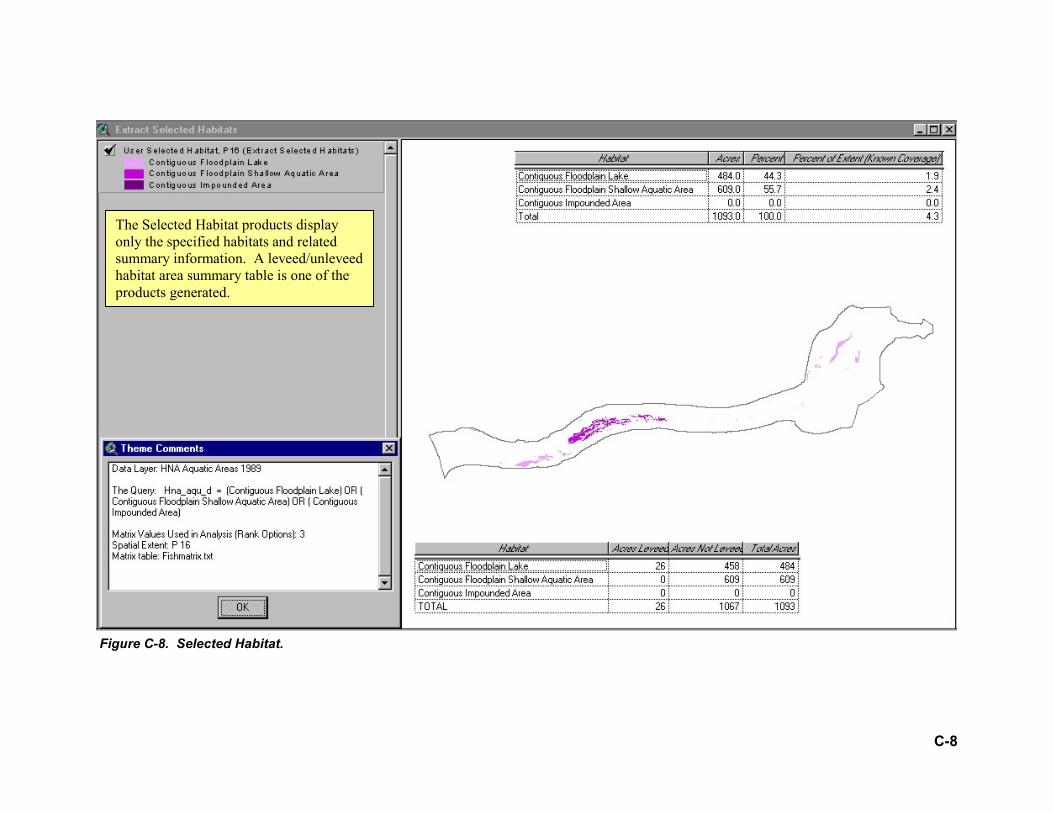
C-8
Figure C-8. Selected Habitat.
The Selected Habitat products display only the specified habitats and related summary information. A leveed/unleveed habitat area summary table is one of the products generated.
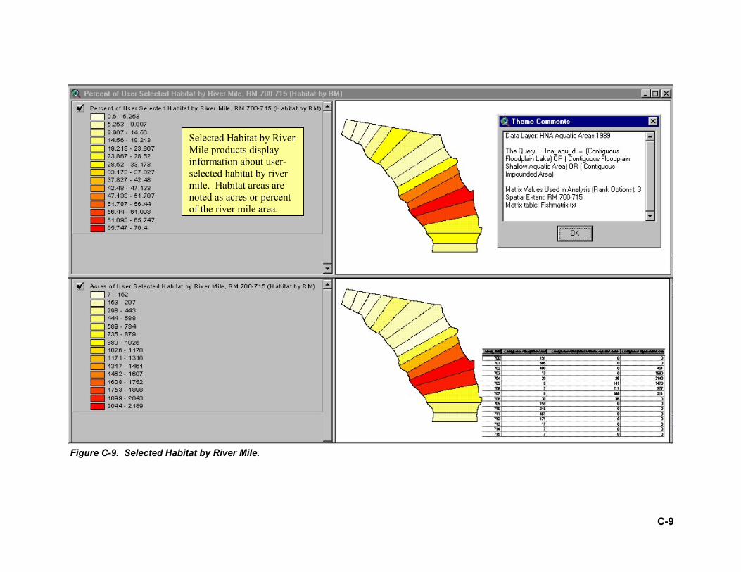
C-9
Figure C-9. Sel ile.
Selected Habitat by River Mile products display information about user-selected habitat by river mile. Habitat areas are noted as acres or percent of the river mile area.
ected Habitat by River M
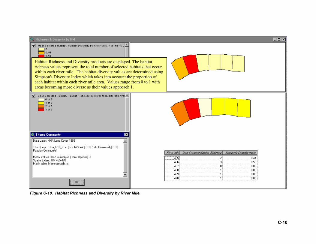
C-10
Figure C-10. Habitat Richness and Diversity by River Mile.
Habitat Richness and Diversity products are displayed. The habitat richness values represent the total number of selected habitats that occur within each river mile. The habitat diversity values are determined using Simpson's Diversity Index which takes into account the proportion of each habitat within each river mile area. Values range from 0 to 1 with areas becoming more diverse as their values approach 1.
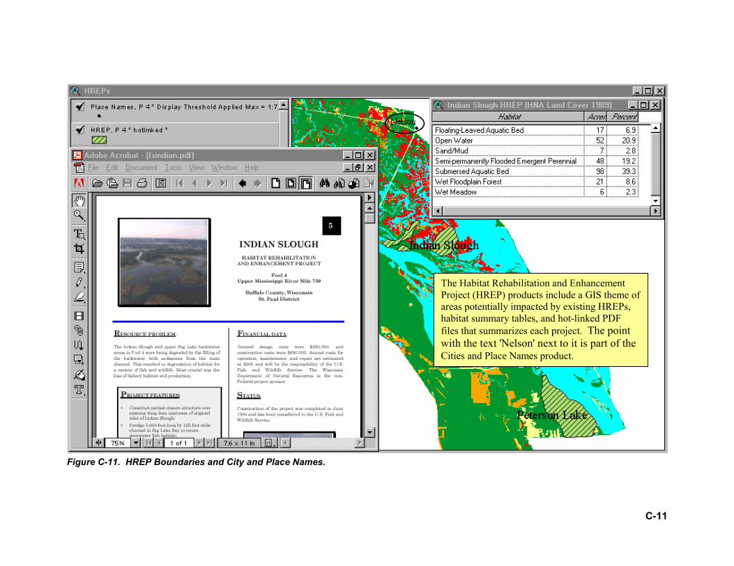
C-11
Figure C-11. HREP Boundaries and City and Place Names.
The Habitat Rehabilitation and Enhancement Project (HREP) products include a GIS theme of areas potentially impacted by existing HREPs, habitat summary tables, and hot-linked PDF files that summarizes each project. The point with the text 'Nelson' next to it is part of the Cities and Place Names product.